a new numerical simulation method for horizontal well in tight
TRANSCRIPT
Journal of Petroleum Science Research, Vol. 4 No. 2‐July 2015 39
2168‐5517/15/02 039‐08, © 2015 DEStech Publications, Inc.
doi: 10.12783/jpsr.2015.0402.01
A New Numerical Simulation Method for
Horizontal Well in Tight Sandstone
Reservoirs Jianchun Xu1, Ruizhong Jiang2, Jianbin Fu*3, Yu Jiang4
1,2,3 China university of Petroleum (East China), 4University of Wyoming
No. 66, Changjiang West Road, Huangdao District, Qingdao, China, 266580
1illeyupc@gmail. com; [email protected], [email protected]; [email protected];
Corresponding Author: *E‐mail:[email protected] (Jianbin Fu)
Equation Chapter 1 Section 1
Abstract
With further progress of oilfieldsʹ development all over the world, more and more tight sandstone reservoirs are being put in
production. The existence of low velocity non‐Darcy flow has been proven, so in this paper the three‐dimensional three‐phase
horizontal well numerical simulator was developed with considering the non‐Darcy flow. The comprehensive comparison and
analysis of the simulation results of Darcy flow and non‐Darcy flow were provided including liquid production rate, oil
production rate, water cut, reservoir pressure, oil saturation distribution and pressure distribution. With considering the
non‐Darcy flow, the fluid flow in reservoir consumes more driving energy, the water flooding efficiency was reduced.
Key words
Horizontal Well; Tight Sandstone Reservoir; Non‐Darcy Flow; Numerical Simulation
Introduction
Over the past decade, the development of unconventional oil and gas has become a hot issue, with more and more
low permeability reservoirs opening to exploration. The low permeability tight sandstone is defined as the
permeability of the matrix is 0.1×10‐3 ~ 10×10‐3 μm2. The flow mechanism of fluid in the low permeability porous
media follows nonlinear flow, and it is significantly different from that of conventional low permeability and high
permeability porous media[1‐5].
The flow curve is a combination of a straight line and a concave curve and the nonlinear flow exists in low
permeability porous media. Pseudo threshold pressure gradient and minimum threshold pressure gradient
exist[6‐8]. Darcy flow model ignores the concave curve segment and the seepage curve is a straight line which goes
through the origin. Quasi‐linear is also a straight line which goes through pseudo threshold pressure gradient spot
in X‐axis. Non‐linear model reflects the real seepage characteristic in low permeability tight sandstone cores[9‐16].
For the tight gas reservoir, the nonlinear flow was also observed in a water‐bearing reservoir. In this paper, the
nonlinear flow reservoir mathematical model is established based on the characteristics of the fluid flow in low
permeability porous media, and the well‐grid equation is deduced[17‐20].
At present, Yang et al.[20‐21] has already established non‐Darcy flow numerical simulator for vertical well, but their
model has no the actual physical meaning. Jiang et al.[22] also has established the low velocity non‐Darcy flow
model with actual physical meaning. However, They both didnʹt consider the horizontal seepage characteristics.
Horizontal well as an important technique has been widely used in recent years in tight sandstone reservoir. Fluid
flow does not follow Darcy’s law in tight sandstone reservoir, so the application of traditional commercial software
in the oilfield development will result in great error, therefore, the development of suitable new software for tight
sandstone reservoir is necessary. On the other hand, although water flooding is a mature secondary recovery
method for conventional reservoirs, it has been applied in tight sandstone reservoirs in a large commercial scale.
Therefore, horizontal well numerical simulation technology is necessary to be established to guide the tight
sandstone reservoir development.

40 JIANCHUN XU, RUIZHONG JIANG, JIANBIN FU, YU JIANG
This paper was organized as following: Firstly, the three‐dimensional three‐phase horizontal well numerical
simulator was developed with considering the non‐Darcy flow. Secondly, the comprehensive comparison and
analysis of the simulation results of Darcy flow with Eclipse were provided. Finally, the development
characteristics of horizontal well was given by comparing the Darcy model, non‐Darcy model and strong
non‐Darcy model.
Numerical Simulation Model for Horizontal Model
Assumption
(1) there are at most three components in reservoir and the oil and water phase obey non‐Darcy’s model ; (2) the
flow is isothermal;(3) the gas can achieve phase equilibrium instantaneously;(4) gravity effect and capillary force
are considered;
Mathematical Model
In tight reservoir the throat in porous media is nano/micro scale, the permeability is changing with the pressure
gradient. Some scholars has put forward some classical models to describe this phenomenon. In order to describe
the non‐Darcy flow curve of tight sandstone reservoir, the low velocity non‐Darcy flow model by Jiang et al. was
used[22].
1) Motion Equation
In matrix, the permeability is low, so the fluids obey non‐Darcy model, and the motion equations are followed:
1
2
(1 )ro oo o
o o o
KKv p
p
(1)
1
2
(1 )rw ww w
w w w
KKv p
p
(2)
rg
g gg
KKV p
(3)
2) The Continuity Equation
Oil component:
o oo o o
Sv q
t
(4)
Water component:
w ww w w
Sv q
t
(5)
Gas component:
od o wd w g g g
od o wd w g g
v v v q
S S St
(6)
3) Numerical Simulation Model
By put the motion equations into continuity equation, the complete numerical simulation model was derived
which is composed of flow equation, boundary conditions and initial condition.
Oil component:

A New Numerical Simulation Method for Horizontal Well in Tight Sandstone Reservoirs 41
1
2
(1 )[ ]ro oo o
o o o o
oov
o
KKp gD
B P
Sq
t B
(7)
Water component:
1
2
(1 )[ ]rw ww w
w w w w
wwv
w
KKp gD
B p
Sq
t B
(8)
Gas component:
1
2
1
2
(1 )
(1 )
so ro oo o
o o o o
sw rw ww w
w w w w
rgg g gv
g g
g so o sw w
g o w
R KKp gD
B p
R KKp gD
B p
KKp gD q
B
S R S R S
t B B B
(9)
4) Auxiliary Equation
Saturation equation:
1o w gS S S (10)
Capillary pressure equation:
cow o w cog g op p p p p p (11)
Initial condition:
0
0
0
, ,
, ,
, ,
w wii
w wii
o oii
p p x y z
S S x y z
S S x y z
(12)
Outer boundary:
Closed boundary
0
0
0
o o
w w
g g
p gD
np gD
n
p gD
n
(13)
Constant pressure boundary

42 JIANCHUN XU, RUIZHONG JIANG, JIANBIN FU, YU JIANG
o
w
g
p const
p const
p const
(14)
Inner boundary condition:
The terms qwwell, qowell,, qgwell, represent water, oil and gas mass production or injection rates at a well. In this
study, Peaceman’s well model was used. The following equation assumes the horizontal well along the x
direction.
2( )
ln( / )
2( )
ln( / )
2( ) ( ) ( )
ln( / )
rw xwwell w wf b
w e w
ro xowell o of b
o e w
rg xgwell g gf b wwell sw owell so
g e w
KK dq P P
r r s
KK dq P P
r r s
KK dq P P q R q R
r r s
(15)
Where bP is the bottom‐hole pressure and er is the effective radius and can be expressed as:
1 2 2 1 2 2 0.5
1 4 1 4
0.2 ,
[( / ) ( / ) ] 0.28
( / ) ( / )y z z ye
y z z y
y y z Ky Kz
K K z K K yr
K K K K
(16)
Where ξ1,ξ2 are non‐Darcy flow coefficients; ν is velocity, m/s; p is pressure gradient, Pa/m; K is permeability,
m2 ; Kr is relative permeability; t is time, s; q is mass production rate, m3/s; ρis density, kg/m3; μ is fluid
viscosity, Pa∙s; S is saturation, dimensionless; φ is porosity, %; B is volume coefficient, m3/m3; Pc is capillary
pressure, Pa; qv is volume production rate, kg/s; x,y,z is cartesian coordinate; P is pressure, Pa; Γ is boundary
domain; o,w,g is oil, water, gas.
Solution
The fully implicit method is adopted to solve these discrete equations, in which the unknowns are solved
simultaneously. The non‐Darcy coefficients are also updated iteration but iteration. Then the non‐Darcy flow
numerical simulation program of three‐dimension and three‐phase in tight sandstone reservoir was compiled.
Illustrative Examples and Results
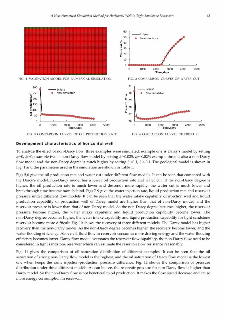
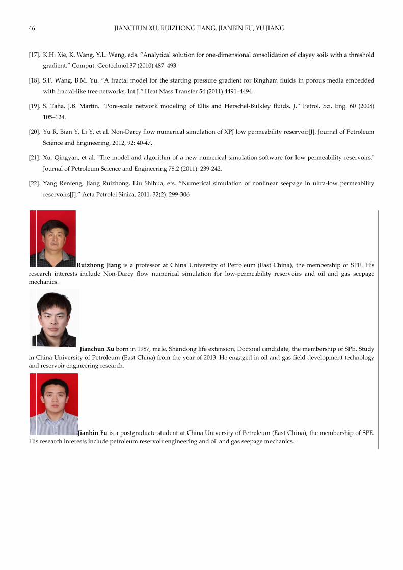
The commercial simulator Eclipse is very famous software in petroleum industry but can’t consider the non‐Darcy
flow. In this model, fluid flow obeys Darcy flow by setting ξ1=0, ξ2=0. As shown in Figs. 2‐4, the results from our
model are in good agreement with Eclipse. The parameters used in the simulation are shown in Table 1.
TABLE 1 PARAMETERS USED IN THE SIMULATIONS
Parameters Value Parameters Value
Reservoir size 600 m*400 m*18 m Water density 1000 kg/m3
Grid member 60*40*9 Oil density 800 kg/m3
Top depth 3000 m Oil viscosity 1 mPa.s
Oil water contact depth 3100 m Water viscosity 0.3 mPa.s
porosity 0.2 Rock compressibility 4 10‐4 M Pa‐1
Horizontal permeability 10 10‐3 2μm Water compressibility 4 10‐4 M Pa‐1
Vertical permeability 10 10‐3 2μm Oil compressibility 4 10‐4 M Pa‐1
Initial pressure 31 MPa Perforating Top layers
Bubble point pressure 10 MPa Well control Pressure keep as a constant
FI
De
To
ξ1=
flo
Fig
Fig
the
hig
bre
pre
pro
res
pre
no
res
rec
wa
eff
con
Fig
sat
on
dis
Da
mo
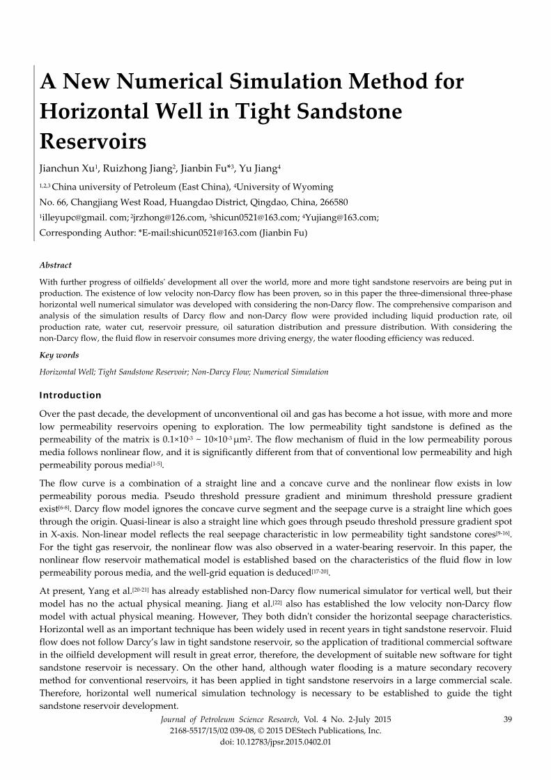
IG. 1 VALIDA
FIG. 3 CO
evelopmen
analyze the
=0, ξ2=0; exam
ow model an
g. 1 and the p
gs 5,6 give th
e Darcy’s mo
gher, the oil
eakthrough t
essure under
oduction cap
servoir press
essure becom
n‐Darcy deg
servoir becom
covery than t
ater flooding
ficiency beco
nsidered in t
g. 11 gives
turation of st
e when kee
stribution un
arcy model. S
ore energy co
0
50
100
150
200
250
300
0
Oil
pro
du
ctio
n,m
3
A New
ATION MODEL
OMPARISON C
nt characte
e effect of no
mple two is
nd the non‐D
parameters u
he oil produc
odel, non‐Da
l production
time become
r different fl
pability of p
sure is lower
me higher,
gree becomes
me more diff
the non‐Darc
g efficiency. A
mes lower. D
tight sandsto
the compari
trong non‐D
ps the same
nder three di
So the non‐D
onsumption
0 1000
EclipNew
Numerical Sim
L FOR NUMER
CURVES OF O
eristics of
n‐Darcy flow
non‐Darcy f
Darcy degree
used in the si
ction rate an
arcy model
n rate is mu
e more behin
low models.
production w
r than that of
the water
s higher, the
ficult. Fig. 10
cy model. As
Above all, flu
Darcy flow m
one reservoir
ison of oil s
Darcy flow m
e injection‐p
ifferent mod
Darcy flow is
in reservoir.
2000 3000Time,days
psew simulator
mulation Method
RICAL SIMULA
IL PRODUCTIO
horizonta
w, three exam
flow model b
is much hig
imulation are
nd water cut
has a lower
uch lower an
nd. Figs 7‐9 g
It can be se
well of Darc
f non‐Darcy
intake capa
water intake
0 shows the r
s the non‐Da
uid flow in r
model oversta
which can e
saturation d
odel is the h
production p
dels. As can b
not benefici
0 4000
d for Horizonta
ATION
ON RATE
al well
mples were s
by setting ξ1=
gher by settin
e shown in T
under differ
r oil product
nd descends
give the wate
een that the
cy model ar
model. As t
ability and
e capability a
recovery of t
arcy degree b
reservoir con
ates the rese
estimate the r
distribution o
highest, and
pressure diffe
be see, the re
ial to oil prod
Wat
er c
ut,
%
5000
al Well in Tight
FIG. 2 COM
FIG. 4 C
simulated: ex
=0.025, ξ2=‐0
ng ξ1=0.1, ξ2=
Table 1.
rent flow mo
tion rate and
s more rapid
er injection ra
water intake
re higher th
the non‐Darc
liquid prod
and liquid p
three differe
becomes high
nsumes more
rvoir flow ca
reservoir flow
of different
the oil satur
erence. Fig.
eservoir pres
duction. It m
0
10
20
30
40
50
60
0 100
Ec
Ne
26
27
28
29
30
31
0P
ress
ure
,MP
a
t Sandstone Res
MPARISON CU
COMPARISON
xample one
.025; exampl
=‐0.1. The ge
odels. It can b
d water cut.
dly, the wat
ate, liquid pr
e capability o
han that of n
cy degree be
duction capa
roduction ca
nt models. T
her, the recov
e driving ene
apability, the
w resistance
examples. I
ation of Darc
12 shows th
ssure for non
makes the flow
00 2000Time,d
lipse
ew simulator
1000 2000T
Eclipse
New simulator
servoirs
URVES OF WA
CURVES OF
is Darcy’s m
le three is al
eological mo
be seen that
If the non‐D
ter cut is m
roduction rat
of injection w
non‐Darcy m
ecomes highe
ability becom
apability for
The Darcy m
very become
ergy and the
e non‐Darcy
reasonably.
It can be se
cy flow mod
he comparis
n‐Darcy flow
w speed decr
3000 400days
0 3000Time,days
r
ATER CUT
PRESSURE
model by sett
lso a non‐Da
del is shown
compared w
Darcy degree
much lower a
te and reserv
well and liq
model, and
er, the reserv
me lower. T
tight sandsto
odel has hig
e lower, and
e water flood
flow need to
een that the
del is the low
son of press
w is higher th
rease and ca
00 5000
4000 5000
43
ting
arcy
n in
with
e is
and
voir
quid
the
voir
The
one
gher
the
ding
o be
oil
west
sure
han
use
0

44 JIANCHUN XU, RUIZHONG JIANG, JIANBIN FU, YU JIANG
FIG. 5 COMPARISON CURVES OF OIL PRODUCTION RATE FIG. 6 COMPARISON CURVES OF WATER CUT
FIG. 7 COMPARISON CURVES OF WATER INJECTION RATE FIG. 8 COMPARISON CURVES OF LIQUID PRODUCTION RATE
FIG. 9 COMPARISON CURVES OF RESERVOIR PRESSURE FIG. 10 COMPARISON CURVES OF RECOVERY
(a) DARCY MODEL (b) NON‐DARCY MODEL (c) STRONG NON‐DARCY MODEL
FIG. 11 RESERVOIR OIL SATURATION DISTRIBUTION OF DIFFERENT FLOW MODELS IN 12 YEARS
(a) DARCY MODEL (b) NON‐DARCY MODEL (c) STRONG NON‐DARCY MODEL
FIG. 12 RESERVOIR PRESSURE DISTRIBUTION OF DIFFERENT FLOW MODELS IN 12 YEAR
0
50
100
150
200
250
300
0 1000 2000 3000 4000
Oil
pro
du
ctio
n r
ate,
m3
Times,days
ξ1=0,ξ2=0ξ1=0.025,ξ2=-0.025ξ1=0.1,ξ2=-0.1
0
10
20
30
40
50
60
0 1000 2000 3000 4000
wat
er c
ut,
%
Times,days
ξ1=0,ξ2=0ξ1=0.025,ξ2=-0.025ξ1=0.1,ξ2=-0.1
0
10
20
30
40
50
60
70
0 1000 2000 3000 4000
wat
er in
ject
ion
rat
e,m
3
Times,days
ξ1=0,ξ2=0ξ1=0.025,ξ2=‐0.025ξ1=0.1,ξ2=‐0.1
0
50
100
150
200
250
300
0 1000 2000 3000 4000L
iqu
id p
rod
uct
ion
rat
e,m
3
Times,days
ξ1=0,ξ2=0
ξ1=0.025,ξ2=‐0.025
ξ1=0.1,ξ2=‐0.1
26
27
28
29
30
31
0 1000 2000 3000 4000
Res
ervo
ir p
ress
ure
,m3
Times,days
ξ1=0,ξ2=0ξ1=0.025,ξ2=‐0.025ξ1=0.1,ξ2=‐0.1
05
10152025303540
0 1000 2000 3000 4000
Rec
over
y,%
Times,days
ξ1=0,ξ2=0ξ1=0.025,ξ2=‐0.025ξ1=0.1,ξ2=‐0.1
X/m
Y/m
0 200 400 600
0
50
100
150
200
250
300
350
400
0.3
0.35
0.4
0.45
0.5
0.55
X/m
Y/m
0 200 400 600
0
100
200
300
400
0.3
0.35
0.4
0.45
0.5
0.55
X/m
Y/m
0 200 400 600
0
100
200
300
4000.3
0.35
0.4
0.45
0.5
0.55
X/m
Y/m
25
25
27
27
27
29
29
29
31
0 200 400 600
0
100
200
300
400
24
26
28
30
X/m
Y/m
23
25
25
27
27
27
29
29
2931
31
0 200 400 600
0
100
200
300
400
24
26
28
30
X/m
Y/m
23
25
25
27
27
27
29
29
29
31
31
0 200 400 600
0
100
200
300
400
24
26
28
30

A New Numerical Simulation Method for Horizontal Well in Tight Sandstone Reservoirs 45
Conclusion
The horizontal well simulator was developed for tight sandstone reservoir considering the non‐Darcy flow. If the
flow is Darcy flow, the results from our model are in good agreement with Eclipse. With considering the
non‐Darcy flow, the fluid flow in reservoir consumes more driving energy, the water flooding efficiency was
reduced.
ACKNOWLEDGMENTS
This work is supported by National Natural Science Foundation of China (Grant No. 51174223 and E0403). Special
thanks are also owed to the editors and reviewers of Journal of Journal of Petroleum Science Research.
REFERENCE
[1]. Huang Yanzhang. ”Nonlinear percolation feature in low permeability reservoir [J].”Special Oil & Gas Reservoirs,
1997,4(1):9‐14.
[2]. Shi Yu, Yang Zhengming, Huang Yanzhang. “Study on nonlinear seepage flow model for low permeability reservoir [J].”
Acta Petrolei Sinica, 2009, 30(5):731‐734.
[3]. Y.D. Yao, J.L. Ge. “Characteristics of non‐Darcy flow in low‐permeability reservoirs.” Petrol. Sci. 8 (2011) 55–62.
[4]. Y.D. Yao, J.L. Ge. “Seepage features of non‐Darcy flow in low‐permeability reservoirs.” Petrol. Sci. Technol. 30 (2012)
170–175.
[5]. S. Taha. “Modelling the flow of yield‐stress fluids in porous media.” Transport Porous Med. 85 (2010) 489–503.
[6]. B. Matthew, S.R. Daniel, K. Alan, eds. “Numerical algorithms for network modeling of yield stress and other
non‐Newtonian fluids in porous media.” Transport Porous Med. (2012).
[7]. H. Pascal. “Nonsteady flow through porous media in the presence of a threshold pressure gradient.” Acta Mech. Sinica 39
(1981) 207–224.
[8]. Y.S. Wu, K. Pruess, P.A. Witherspoon. “Flow and displacement of Bingham non‐Newtonian fluids in porous media.” SPE
Reservoir Eng. 7 (1992) 369–376.
[9]. WANG En‐zhi, HAN Xiao‐mei, HUANG Yuan‐zhi. “Discussion on the mechanism of percolation in low permeability
rocks [J]. “Rock and Soil Mechanics,2003, Sup2:120‐125.
[10]. CHENG Shiqing, XU Lunxun, ZHANG Dechao. “Type curve matching of well test data for non‐darcy flow at low velocity
[J].”Petroleum Exploration and Development, 1996,23(4):50‐53.
[11]. Yao Jun, Liu Shun. “Well test interpretation model based on mutative permeability effects for low‐permeability
reservoir[J].” Acta Petrolei Sinica,2009,30(3):430‐433.
[12]. J. Bear. “Dynamics of Fluids in Porous Media.” Dover Publications Inc., New York, 1972.
[13]. A. Prada, F. Civan, “Modification of Darcy’s law for the threshold pressure gradient, J.” Pet. Sci. Eng. 22 (1999) 237–240.
[14]. S.J. Wang, Y.Z. Huang, F. Civan. “Experimental and theoretical investigation of the Zaoyuan field heavy oil flow through
porous media, J.” Petrol. Sci. Eng. 50(2006) 83–101.
[15]. F. Hao, L.S. Cheng, O. Hassan, eds. “Threshold pressure gradient in ultra‐low permeability reservoirs.” Pet. Sci. Technol.
26 (2008)1035–1204.
[16]. W. Xiong, Q. Lei, S.S. Gao, eds. “Pseudo threshold pressure gradient to flow for low permeability reservoirs.” Petrol.
Explor. Dev. 36 (2009) 232–236.
46
[17
[18
[19
[20
[21
[22
res
me
in C
and
His
7]. K.H. Xie, K
gradient.” C
8]. S.F. Wang,
with fractal
9]. S. Taha, J.B
105–124.
0]. Yu R, Bian
Science and
]. Xu, Qingya
Journal of P
2]. Yang Renfe
reservoirs[J
search interest
echanics.
China Univer
d reservoir en
s research inte
K. Wang, Y.L. W
Comput. Geot
B.M. Yu. “A
l‐like tree netw
B. Martin. “Po
Y, Li Y, et al.
d Engineering,
an, et al. ʺThe
Petroleum Scie
eng, Jiang Ru
J].” Acta Petro
Ruizhong Ji
ts include No
Jianchun X
rsity of Petrole
gineering rese
Jianbin Fu i
erests include
JIANCHUN
Wang, eds. “A
technol.37 (20
fractal mode
works, Int.J.“ H
ore‐scale netw
Non‐Darcy fl
, 2012, 92: 40‐4
e model and a
ence and Engi
uizhong, Liu S
olei Sinica, 201
iang is a prof
on‐Darcy flow
Xu born in 198
eum (East Chi
earch.
is a postgradu
petroleum res
N XU, RUIZHO
Analytical solu
10) 487–493.
l for the start
Heat Mass Tra
work modelin
low numerica
47.
algorithm of a
ineering 78.2 (
Shihua, ets. “N
11, 32(2): 299‐3
fessor at Chin
w numerical
87, male, Shan
ina) from the
uate student a
servoir engine
ONG JIANG, J
ution for one‐d
ting pressure
ansfer 54 (2011
ng of Ellis and
al simulation o
a new numeri
(2011): 239‐242
Numerical sim
306
na University
simulation fo
ndong life exte
year of 2013.
at China Univ
eering and oil
JIANBIN FU,
dimensional c
gradient for B
1) 4491–4494.
d Herschel‐Bu
of XPJ low per
ical simulation
2.
mulation of n
of Petroleum
or low‐permea
ension, Doctor
He engaged i
ersity of Petro
and gas seepa
YU JIANG
onsolidation o
Bingham fluid
ulkley fluids,
rmeability res
n software for
nonlinear seep
m (East China)
ability reservo
ral candidate,
in oil and gas
oleum (East C
age mechanics
of clayey soils
ds in porous m
J.” Petrol. Sc
servoir[J]. Jour
r low permea
page in ultra‐l
), the member
oirs and oil
the membersh
field develop
China), the me
s.
s with a thresh
media embed
ci. Eng. 60 (20
rnal of Petrole
bility reservoi
low permeabi
rship of SPE.
and gas seep
hip of SPE. Stu
pment technol
mbership of S
hold
ded
008)
eum
irs.ʺ
ility
His
page
udy
logy
SPE.

Journal of Petroleum Science Research, Vol. 4 No. 2‐July 2015 47
2168‐5517/15/02 047‐19, © 2015 DEStech Publications, Inc.
doi: 10.12783/jpsr.2015.0402.02
Optimization of Infill OilWell Locations Field‐Scale Application
Watheq Al‐Mudhafar*1&Mohammed Al‐Jawad2
1Department of Petroleum Engineering, Louisiana State University, Baton Rouge, LA 70803, USA
2Petroleum Technology Department, University of Technology, Baghdad, Iraq
*[email protected]; +1.225.715.2578
Abstract
Determining the optimal locations of infill wells is a crucial decision to be made during a field development plan. It concerns
implementing accurate reservoir modelling in order to precisely evaluate the reservoir behavior and predict its future
performance. The reservoir modelling‐optimization approaches were adopted on the main pay‐Upper Sandstone formation of
South Rumaila Oil Field, located in Iraq. First of all, comparing outcomes of different parameters with their measured values
through history matching process attained the validity of the reservoir flow model. After that, two methods of optimization
were adopted to find out the optimal number and locations of infill oil wells.The first method is manual optimization via
spreadsheet and the second one is automatic optimization throughAdaptive Genetic Algorithm (GA). Both methods were done
according to the aspects of net present value (economic evaluation) as objective function in the wells selection optimization
procedures. GA depends on the principle of artificial intelligence concept of Darwin’s theory of Natural Selection. The genetic
program was coupled with the reservoir flow model to re‐evaluate the chosen wells at each iteration until obtain the optimal
choice. The genetic algorithm program gave results similar to the results that were obtained by manual method with much less
computation time. Three different future predictions of oil production and NPV cases were studied to determine the optimal
future scenario with respect to whether considering water injection or not in the available water injectors. The first one without
water injection, the second and third with 7500 surface bbls/day and 15000 surface bbls/day water injection per well,
respectively. According to the relationship between net present value and future production time, the abandonment time was
estimated to be at the end of the 8th prediction year for all above cases. The optimal future scenario was with water injection of
15000 surface bbls/day; however, the current capabilities of surface injection facilities cannot handle this rate. Therefore, the
optimal future prediction is to continue with water injection of 7500 surface bbls/day/well. The optimal number of infill wells
for this case was three wells even though drilling more wells have led to increase the cumulative oil production. The
incremental percent of NPV based on the optimized infill well location scenario are improved by 3.4% higher than the base case
on no‐infill wells.
Keywords
Developed Reservoir; Optimal Future Performance; Optimal Infill Well Locations;Adaptive Genetic Algorithm; Economic Analysis;
Optimal Number of Infill Wells
Introduction
The main objective of the integrated reservoir studies is to figure out the optimal future performance in order to
improve oil recovery, precisely with considering the economical evaluation. Determination of optimal number and
locations of infill wells is one of the most important scenarios that help improve the cumulative oil production and
Net Present Value (NPV). The Solution of this kind of problems encompasses two main entities: The field
production system and the geological reservoir. Each of these entities presents a wide set of decision variables and
the choice of their values given different constrains is an optimization problem.
In the current research, the determination of optimal infill oil well locations is a complex task because it is affected
by many factors such as reservoir and fluid properties in addition to the interference between the wells.
Sometimes, drilling new wells may affect the production of other wells. Also the optimal additional well locations
depend on well and surface equipment specifications, as well as the economic parameters. Therefore, the aim is to
find a development strategy that maximizes the revenue after running the reservoir model to the abandonment
time of production.
The reservoir flow simulation is a conventional way to evaluate most of the factors that might affect the future

48 WATHEQ AL‐MUDHAFAR&MOHAMMED AL‐JAWAD
reservoir performance considering the optimal new well locations. The numerical simulator has been used as an
evolution function to test different future performance scenarios and different infill well number and locations. The
presented optimization techniques have been applied for determining the optimal infill well locations based on net
present value (NPV) as objective function. Net present value is a function of economic variables representing costs
and revenues. The revenue is directly proportional to the cumulative oil production, which is predicted by
reservoir model. The costs include capital (CAPEX) and operational (OPEX) expenditures. Manual optimizations
via spreadsheet and automatic procedure through genetic algorithm technique have been adopted in the current
study through a field‐scale application on a sector in South Rumaila Oil Field.
Description of South Rumaila Oil Field
The Rumaila oil field is located in south of Iraq, about 50 km west of Basrah and about 30 km to the west of the
Zubair field (Al‐Ansari 1993). The field is associated with large gentle anticline fold of submeridional trend. The
dimensions of South Rumaila Oil Field are about 38 Km long and 12 Km wide. The upper sandstone member of the
Zubair formation is the main pay zone of South Rumaila Oil Field. The Zubair formation in south of Iraq (Rumaila,
West Qurna and Zubair Fields) belongs to the depositional cycle of Lower Barremian to Aptain of Lower
Cretaceous age (Al‐Ansari, 1993). The formation is generally composed of sandstone and shale. The ratio of sand in
the formation decreases significantly northeastwhile this ratio increases southwest of the field. The Zubair
formation has been divided into five members on the basis of sand to shale ratio and these have been named from
top to bottom the following: Upper shale member, Upper sandstone member (main pay), Middle shale member,
Lower sand member, and Lower shale member.
The main pay is the Upper sandstone member and it comprises three dominated sandstone units, separated by two
shale units. The shale units act as good barriers impeding vertical migration of the reservoir fluids except in certain
areas where they disappear.
The South Rumaila Field is divided into four production sectors. From north to south, the sectors are Qurainat,
Shamia, Rumaila, and Janubia. The sector studied most closely is the Rumaila sector, along with small parts from
the Shamia and Janubia sectors. The choice of this sector was made specifically because it is the largest sector in
which the production and injection operations are carried out as shown in Fig. 1.
FIG. 1 WELL LOCATIONS FOR THE SECTOR UNDER STUDY IN SOUTH RUMAILA OIL FIELD (AL‐MUDHAFER, 2013)

Optimization of Infill OilWell Locations 49
Black Oil Reservoir Model
The black oil reservoir simulator has been adopted for reservoir evaluation and predicting the future field
performance.
The constructed grid in the current model includes the reservoir and parts of infinite active edge‐water aquifer
along the eastern and western flanks. The 3Dreservoir model is performed over 15 x 11 x 5 grids in the I, J, and K
directions, respectively. The reservoir in the vertical direction is divided into five vertical layers (Al‐Mudhafer et
al., 2010). The 15 x 11 x 5 grid models contained 825 cells. Of these, (584) cells or (70.8%) are active. The gridblocks
areal dimensions are uniform and equal to (1000m x 866m). The orthogonal corner geometry has been considered
for grid construction in this model. According to the cumulative probability function of horizontal permeability
distribution, the reservoir has very heterogeneous rocks, since the heterogeneity index (Dykstra‐Parsons
Coefficient) is around 60%. The vertical permeability within each layer was assumed to be one tenth of the
horizontal permeability at each grid blocks (Al‐Ansari, 1993).
The reservoir properties such as porosity, permeability, and layersʹ thickness have been obtained from previous
studies on this field (Al‐Mudhafer et al., 2010). The physical and thermodynamic properties of the reservoir’s fluids
have been obtained based on previous analyses of large number of oil samples taken from large number of wells
through more than fifty years (Al‐Mudhafer et al., 2010). The reservoir oil is undersaturated since the initial and
current reservoir pressure is greater than the unique bubble point pressure that exists throughout the reservoir.
The bubble point pressure is 2660 psi while initial reservoir pressure of 5186 psi measured at 3154.7m datum. The
current average reservoir pressure is 4200 psi and the original oil‐water contact (OWC) is 3269m. Although the
reservoir is highly heterogeneous, only two rock types have been adopted for capillary pressure and relative
permeability curves since most of the permeability values among the spatial distribution have been assigned to
these typesʹ ranges. The coarse sand is located within 400‐800md and the medium coarse sand is ranged from 100‐
400md.
The simulation time for the current study is 60 years from 1954 to present. During that period, 40 production wells
were opened to flow in the simulated domain. The production of some layers was ceased because of the higher
water cut values, especially from the lower layers. For more than two decades, depletion and water drive have
been the only production mechanisms. After that a pressure maintenance was carried out by drilling 20 water
injection wells at the east flank, just to maintenance the pressure from the west flank because the aquifer’s strength
from the west flank is about 20 times its strength from the east one (Kabir, 2007). The northern and southern
boundaries are assumed to be a no‐flow. This assumption may be considered realistic since the direction of flow at
each of the five layers was towards the reservoir crest and parallel to the northern and southern edges.
Furthermore, the northern and southern streamlines at the isobaric contour maps are perpendicular to these
boundaries (Al‐Mudhafer et al., 2010). The boundaries at the east and west are under the infinite acting water drive
aquifer.
To achieve a matching acceptable history, many runs have been carried out in order to get a minimum error
between the calculated and observed values. This process encompasses matching of average reservoir pressure
jointly with overall reservoir saturation. The saturation matching has been done based on the available water cut
and initial time of breakthrough for some wells in different time.
The best matches obtained involve the following steps of modifications: ‐
1. Assuming the average reservoir pressure equals to 5186 psia at datum level of 10350 ft. BSL or 3154 m,
which has been obtained from previous field literature.
2. Modifying the following properties of the reservoir and aquifer:
a) Multiply the transmissibility of the 1st layer at the eastern flank by 1.3.
b) Multiply the transmissibility of the 2nd& 3rdlayers at the eastern flank by 1.5.
c) Multiply the transmissibility of the 4th& 5thlayersat the eastern flank by 2.0.
d) Multiply the aquifer size by 3.0.
3. Because of the lack of well status for nine wells, the production from these wells are assumed first to be

50 WATHEQ AL‐MUDHAFAR&MOHAMMED AL‐JAWAD
from all five layers and then some modifications in completion of these wells have been made by plugging
the bottom layers that assumed to be completely flooded by water.
The calculated average reservoir pressure values are compared with the measured average reservoir pressure. The
best match of average reservoir pressure is given in Fig. 2.
The reasonable match of saturation indicates correct fluid movements through the reservoir.The initial
breakthrough is the time when the value of water cut approaches 10%. The comparisons, with respect to the water
cut and the breakthrough times, have been done according to Mohammed’s, Hamdullah’s, and Franlab studies (Al‐
Mudhafer et al., 2010). These calibrations, present in Table 1 show the water cut matching for 10 wells and in Table
2, which has the breakthrough time matching for five wells.
FIG. 2 CALCULATED AND MEASURED AVERAGE RESERVOIR
PRESSURE MATCHING
TABLE 1 WATER CUT MATCHING
Well Date
Water Cut
(%)
Franlab
Study, 2010
Water Cut (%)
Hamadallahʹs
Study, 1999
Water Cut
(%)
Current
Model
1 10/98 0.0 0.0 0.0
2 1/98 0.3 0.1 0.5
3 4/98 0.0 0.08 0.0
4 9/98 0.0 0.0 0.0
5 9/98 4.4 1.0 3.1
6 6/2001 10.9 ‐ 10.6
7 3/2004 0.5 ‐ 0.0
8 7/2003 0.05 ‐ 0.0
9 3/2004 6.0 ‐ 5.0
10 1/2003 0.18 ‐ 0.0
TABLE 2TIME OF WATER BREAKTHROUGH
TIME OF INITIAL BREAKTHROUGH
WELL MEASURED CURRENT MODEL MOHAMMED’S STUDY
11 19/4/72 31/11/69 1/10/72
12 1/3/88 31/1/88 1/11/88
13 21/9/61 31/12/62 21/5/61
14 3/5/88 31/7/89 4/2/89
15 9/6/2001 30/11/2000 ‐
Optimization Procedure
In petroleum engineering, the objective function is commonly the cumulative oil production or the net present
value over a certain future prediction period (Güyagüler, 2000). The decision variables in a given problem may
have significant influence on oil production history and the potential profit; therefore, they need to be optimized.
Based on the problem or some prior practical analysis, the range limit (levels) of the decision variables should be
determined in order to justify the optimization space for these variables. After the objective function and all the
decision variables are determined, the optimization problem can be formulated as a maximization or minimization
problem subjected to certain constraints (Phillips, 1976). All the above terms were considered in this research for
the optimization of infill well locations.
Objective Function
In this work, the objective function is the net present value given the flow response. The net present value is one of
the applications of cash flow model (Mian, 1992). The cash flow (future income) analysis provides the value of the
objective function for a specific combination of the decision parameter values considered for the optimization task.
So, each set of decision parameters, p = (p1, p2,…, pn) is associated with a cash flow value C, or
C f p (1)
3000
3500
4000
4500
5000
5500
1950 1960 1970 1980 1990 2000 2010
Production Time, YEAR
Pre
ssu
re, P
SIA
Calculated Average Reservoir Pressure, PSIA
Measured Average Reservoir Pressure, PSIA

Optimization of Infill OilWell Locations 51
The current study incorporates revenues such as oil and gas sales, as well as expenses such as operation, water
handling and injection costs in addition to the capital expenditures of drilling and completion costs (Badru, 2003).
Decision Variables
The decision variables in the current problem are the (i, j) coordinates. They represent the number of the wells to be
drilled and the number of wells. The dimensions of the problem depend on the number of wells. Since each well
has two variables to be optimized that are i and j, the dimension of the problem is equal to power the number of
wells, i.e. when the number of optimized wells is 10; the number of iterations is 1024 (210=1024).
Constraints
The constraints for the current study are the well constraints such as water cut (WC) =0.45, gas‐oil ratio (GOR) =
800 SCF/STM, and bottom hole pressure (BHP) =2700 psia. The other constraints are the locations of the old wells;
the locations in east and west flank from the aquifer; and no more than one well placed in each grid.
Net Present Value formulation
The net future value is defined as the revenues from produced oil and gas sales, after subtracting the costs of
capital expenditures (CAPEX), operational expenditures (OPEX) in addition to costs of disposing produced water
and cost of injecting water (Ozdogan, 2004; Nwaozo, 2006). The result is the net cash flow: ‐
g w injNet Cash Flow =Q Oil Price+ Q Gas Price-Q WH Cost-Q WI Cost-OPEX-CAPEXot t t t t (2)
Where: ‐
Oil price: ($ per STB).
Gas price: ($ per MSCF).
Water handling cost: ($ per bbl.).
Water Injection Cost: ($ per bbl.).
Eq. (2) represents the net cash flow after a given period, which is Net Future Value (NFV).
The prices of oil and gas and the cost of water injection are assumed to be constant over the project life (Nwaozo,
2006). The oil and gas prices were assumed to be $60 per STB oil and $3 per MSCF gas, respectively. This level of
oil price is adequate for the light Iraqi oil for long‐tem production periods since 2003, except the high rate in
previous two years. We considered this low oil price level in order to capture the high certain net present value
estimation.
OPEX: ‐ the operational expenditures include Staff Costs, Daily Energy Requirements, Transportation tariffs, Work
over operations, Maintenance, and Facility upgrades(Johnston, 2003). OPEX was assumed to be 1.5$ per barrel in
this study.
CAPEX: ‐ the capital expenditures include the following items (Johnston, 2003): ‐
1) Initial Investments regarding the drilling, completion, cementing, perforation, acidizing services, and rig
movement operations between well locations.
2) Materials, which include: ‐
a) Tangible such as well head, casing & casing accessories, pipelines, cement & cement add and
completion materials and equipments.
b) Non‐Tangible such as bit, mud material, perforating material charges and accessories, acid material.
Eq. (2) must be discounted into net present value (NPV) by using the mathematical relationship between future
value, present value, and interest rate as shown by the following equation (Ozdogan, 2004):
FV PVi
PV
(3)
FV=PV (1+i) at 1st year or

52 WATHEQ AL‐MUDHAFAR&MOHAMMED AL‐JAWAD
)t
FVPV
(1 i
(4)
Eq. (4) can be written in the following form:
1
tt
NCF tNPV
i
(5)
Where:
NPV: net present value.
NCF: net cash flow.
FV: future income value.
PV: present income value.
t: the future time that at which NPV calculated.
i: the interest rate.
The interest rate (i) is “the interest paid or received on the original principal regardless of the number of time
periods that have passed or the amount of interest that has been paid or accrued in the past” (Bittencourt, 1997).
Manual Optimization
The main aim from oil field development is to increase net present value (NPV). One of the methods for increasing
NPV is drilling additional oil production wells in the field. So this aim highly depends on the number of wells that
would be drilled and the well locations (Beckner, 1995). The proposed infill well locations can be specified
according to the contour maps of permeability and oil saturation at the last simulation timestep. These contour
maps are the best indicator for determining the best and worst locations to drill infill wells (Badru, 2003).These
maps were obtained by using a criterion that characterizes each gridblock in a quantitative manner for the
suitability of the well (Güyagüler, 2002).
_ _ , , ,oTARGET WELL LOCATION f S x y k x y (6)
The high values of the last function on the map indicate the probable promising locations. The low values indicate
locations where an infill is not recommended. After determining the possible infill well locations, optimization
technique should be adopted to determine the optimal number and locations of infill wells (Quenes, 1994). The
main steps of manual optimization are:
1. Run the reservoir model to a specific future period with proposition one new oil well that has higher
permeability and oil saturation.
2. Calculate the net present value based on cumulative oil, gas, and water production.
3. Run the simulator while assuming two new oil wells that have higher permeability and oil saturation and
calculate the net present value (NPV).
4. Continuing with proposition new wells according to this aspect in additive way until they reach 20 wells in
the locations that represent the region that may have promising oil, according to the mentioned contour
maps of permeability and oil saturation.
5. Plot the relationship between the numbers of proposed wells in additive way versus the Net Present Value,
and then the optimal number of wells has the highestNPV.
Optimum Abandonment Time
Before determining the optimal number and locations of wells, the optimum abandonment time for the field with
infill drilling should be determined. The abandonment year is selected by finding the year that maximizes the net
present value (Beecroft, 1999).

Optimization of Infill OilWell Locations 53
An Introduction to Genetic Algorithm
Genetic Algorithms (GA) offer an efficient search technique and can be used as powerful optimization tools as
introduced by John Holland in 1975 (Goldberg, 1989). The population encompasses potential solutions generated
randomly (represented by chromosomes) to a problem, which compete with each other in order to achieve
increasingly better results by applying a set of operators: Selection, Crossover (Recombination), and Mutation.
These operators mimic the genetic reproduction in biological sense similar to Darwin’s theory of Natural Selection
(Goldberg, 1989).
There are several applications of genetic algorithms in petroleum and natural gas industry, mainly as optimization
tools. The first application in the literature goes back to one of Holland’s students named David Goldberg. He
applied a genetic algorithm to find the optimum design for gas transmission lines (Mohaghegh, 2001). Also,
Genetic algorithms have been used in reservoir characterization (Romero, et al., 2000; Mohaghegh, et al., 1994;
Romero, et al., 2000) and the stimulation candidate selection in tight gas sands (Mohaghegh, et al., 2000). In
addition, GA was adopted into the distribution of gas‐lift injection (Martinez, et al., 1994), Petrophysics (Fang, et
al., 1992), and well test analysis (Yin, et al., 1998; Guyaguler and Horne, 2001). Furthermore, it was used in
hydraulic fracturing design (Mohaghegh, et al., 1996; Mohaghegh, et al., 1999), determining the Value ofReservoir
Data (Palke and Horne, 1997)& modelling (Sen, et al., 1992), and Nonconventional Well Deployment (Artus, et al.,
2004). GA has been utilized in many other petroleum problems (Mohaghegh, et al., 1998; Fichter, 2000, Bittencourt,
1994; Guerreiro, et al., 1997;Al‐Mudhafer, 2013).
Basic Terminology
Genetic Algorithms use a specific terminology with some terms derived from genetics as found in the biological
sciences. Below is a list of the definitions of some terms in the GA vocabulary (Austin, 1990): ‐
Population: Set of individuals representing possible solutions in the optimization problem.
Generation: Iteration level within the optimization.
Fitness: Objective function.
Fittest: Solution with highest objective function within a generation.
Chromosome: Encoded string representing an individual solution.
Allele: Building block (bits) of chromosomes and also referred to as genes.
Parents: A couple of individuals (solutions) selected for reproduction.
Children (offspring): Resulting individuals after the reproduction.
In the current study, each well represents one gene in the chromosome. The chromosome consists of eight genes
(most probable target well locations according to the contour maps and manual optimization outcome), i.e. each
chromosome represents the total number of wells to be optimized. The initial population would be a collection of
non‐limited number of the chromosomes. Actually, the number of chromosomes in the initial population is nearly
equal or more than the number of optimized wells(Jefferys, 1993).
Encoding methods
The decision variables in the current study are the number and locations of proposed wells. The true
representation of well locations according to their dimensions is called phenotype. These wells and their number
should be converted to genetic terms (genotype) by binary encoding. The types of encoding are binary, integer, and
real valued etc. (Goldberg, 1989).The genetic algorithm starts with creating initial population of chromosomes. The
length of chromosome is equal to the number of proposed wells. Each chromosome consists of eight genes
(proposed wells). If the well is selected, the encoding will be 1, if not it will be 0. The selection of genes takes place
randomly (Schmidt and Stiden, 1997; Jefferys, 1993).
Population and Initialization
A population consists of a number of individuals each representing a solution for a given problem. This number

54 WATHEQ AL‐MUDHAFAR&MOHAMMED AL‐JAWAD
called population size. A designer of the GAs chooses it. Every chromosome consists of genes that are often
referred to as the genotype while the decoding creates phenotype based on a genotype. Initialization of a
population of individuals is generally a simple operation where if a heuristic is available for producing good
solution; however, the initial population are randomly generated (Goldberg, 1989;Grant, 1995).
Evaluation
Having decoded the chromosome representation into the decision variable domain, it is possible to assess the
performance, or fitness, of individual members of a population. This is done through an objective function that
characterizes an individual’s performance in the problem domain. In the natural world, this would be an
individual’s ability to survive in its present environment. Thus, the objective function establishes the basis for
selection of pairs of individuals that will be mated together during reproduction (Da. Ruan, 1997; Austin, 1990).
Selection
Selection is a genetic operator that chooses a chromosome from the current generation’s population for inclusion in
the next generation’s population. There are two types of the most common selection schemes:
1. Roulette Wheel Selection: a typical selection method. The probability to be a winner is proportional to the area
assigned to an individual on the roulette wheel. From this analogy, the roulette wheel selection gives the selection
probability to individuals in proportionto their fitness values.
1
iselection all
ii
F xP i
F x
Where:
Fi: fitness of individuals.
Pselection: selection probability.
2. Tournament Selection: a number of individuals are randomly selected and their fitness values compared, the one
with higher fitness selected as a parent, if their fitness values are equal one of them is randomly chosen. This
method has been adopted in the current GA model.
Crossover / Recombination
Crossover combines (mates) two chromosomes (parents) with probability (Pc) to produce a new chromosome
(offspring). The idea behind crossover is that the new chromosome may be better than both of the parents if it takes
the best characteristics from each of them. There are several popular combination methods (Goldberg, 1989;Austin,
1993; Grant, 1995; Mitchell, 1996; Schmidt and Stiden, 1997; Jefferys, 1993): ‐
1. One Point crossover (1x): this type chooses one crossover site at a random position within parent and
exchange genes after the crossover site.
2. Two Point Crossover (2x): chooses two‐crossover sites at a random position within parent and exchange
genes between these two crossover sites.
3. Uniform Crossover (UX): randomly shuffles the genes of the chromosomes to create two offspring. This type
was adopted in the current program.
Mutation
Mutation is a random change of one or more genes(Da. Ruan, 1997). This can result in entirely new gene values
being added to the gene pool. Every chromosome is simply scanned gene by gene and with a mutation rate (Pm) a
gene is changed / swapped, i.e. 0 to 1 and 1 to 0. The probability for a mutation is usually kept small, such that we
can expect one muted gene per chromosome.
Optimization of Infill OilWell Locations 55
Replacement Policy
The Replacement operator removes few relatively poor individuals from populations and replaces it with offspring
that have higher fitness (Goldberg, 1989;Jefferys, 1993). There are many replacement operators such as:
1. Holland method: The offsprings are replaced with poor individuals in the population without comparing
the fitness of them.
2. Tournament method: Two (or three) individuals are randomly chosen from the population; the worse of
them is compared with the offspring and if it is the worst, it is then replaced. This type is used in the
present program.
Stopping criteria
There are many different ways to determine when to stop running the GA and return the best solution. One
method is to stop after a given number of generations and this criterion has been adopted in the current program.
The maximum number of generations currently is one hundred (Maxgen=100). Another technique is to stop after
the GA has converged; that is, all individuals in the population are identical. The GA can also be halted if the
solution quality of the population does not improve within a specified number of generations.
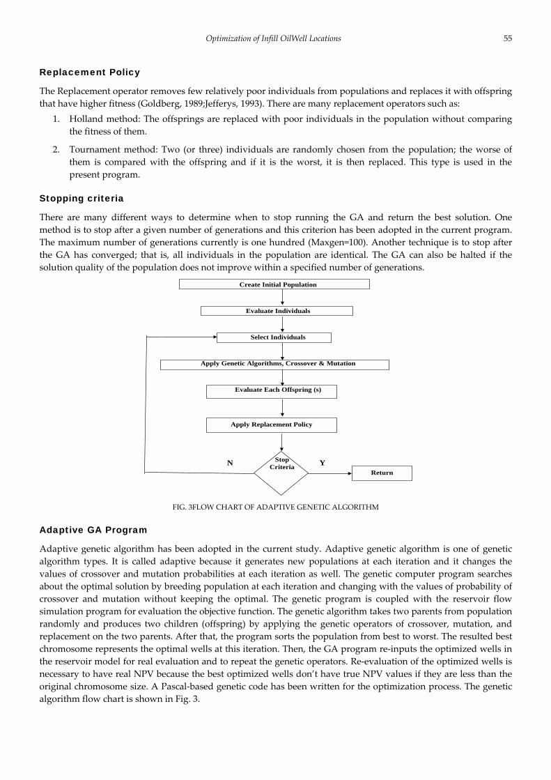
FIG. 3FLOW CHART OF ADAPTIVE GENETIC ALGORITHM
Adaptive GA Program
Adaptive genetic algorithm has been adopted in the current study. Adaptive genetic algorithm is one of genetic
algorithm types. It is called adaptive because it generates new populations at each iteration and it changes the
values of crossover and mutation probabilities at each iteration as well. The genetic computer program searches
about the optimal solution by breeding population at each iteration and changing with the values of probability of
crossover and mutation without keeping the optimal. The genetic program is coupled with the reservoir flow
simulation program for evaluation the objective function. The genetic algorithm takes two parents from population
randomly and produces two children (offspring) by applying the genetic operators of crossover, mutation, and
replacement on the two parents. After that, the program sorts the population from best to worst. The resulted best
chromosome represents the optimal wells at this iteration. Then, the GA program re‐inputs the optimized wells in
the reservoir model for real evaluation and to repeat the genetic operators. Re‐evaluation of the optimized wells is
necessary to have real NPV because the best optimized wells don’t have true NPV values if they are less than the
original chromosome size. A Pascal‐based genetic code has been written for the optimization process. The genetic
algorithm flow chart is shown in Fig. 3.
Create Initial Population
Evaluate Individuals
Select Individuals
Apply Genetic Algorithms, Crossover & Mutation
Evaluate Each Offspring (s)
Stop Criteria
N
Apply Replacement Policy
Return
Y
56 WATHEQ AL‐MUDHAFAR&MOHAMMED AL‐JAWAD
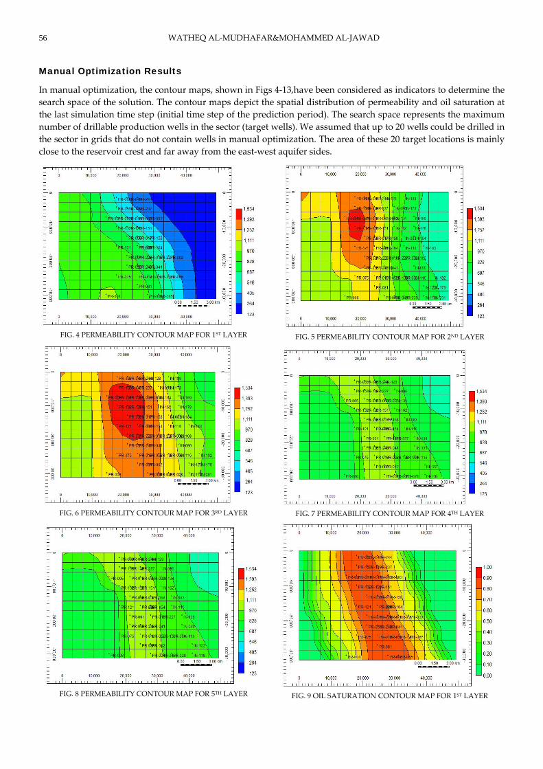
Manual Optimization Results
In manual optimization, the contour maps, shown in Figs 4‐13,have been considered as indicators to determine the
search space of the solution. The contour maps depict the spatial distribution of permeability and oil saturation at
the last simulation time step (initial time step of the prediction period). The search space represents the maximum
number of drillable production wells in the sector (target wells). We assumed that up to 20 wells could be drilled in
the sector in grids that do not contain wells in manual optimization. The area of these 20 target locations is mainly
close to the reservoir crest and far away from the east‐west aquifer sides.
FIG. 4 PERMEABILITY CONTOUR MAP FOR 1ST LAYER
FIG. 5 PERMEABILITY CONTOUR MAP FOR 2ND LAYER
FIG. 6 PERMEABILITY CONTOUR MAP FOR 3RD LAYER
FIG. 7 PERMEABILITY CONTOUR MAP FOR 4TH LAYER
FIG. 8 PERMEABILITY CONTOUR MAP FOR 5TH LAYER
FIG. 9 OIL SATURATION CONTOUR MAP FOR 1ST LAYER

Optimization of Infill OilWell Locations 57
FIG. 10 OIL SATURATION CONTOUR MAP FOR 2ND LAYER
FIG. 11 OIL SATURATION CONTOUR MAP FOR 3RD LAYER
FIG. 12 OIL SATURATION CONTOUR MAP FOR 4TH LAYER
FIG. 13 OIL SATURATION CONTOUR MAP FOR 5TH LAYER
Proposed Future Production Schemes
To accomplish the objective of this study, the future reservoir behaviorunder different production scenarios has
been evaluated. Therefore, 15 production‐injection schemes with respect to water injection rates and number of
infill wells have been assumed to mainly determine whether to have future water injection scenario in the infill
well optimization or not. The main procedure starts by running the reservoir simulator with proposing 0, 5, 10, 15,
& 20 infill production wells in the following three cases:
Case1. Run the simulator with no water injection.
Case2. Run the simulator with 7500 surface bbls/day water injection per each injection well.
Case3. Run the simulator with 15000 surface bbls/day water injection per each injection well.
The field sector consists of 60 wells, from which 40 oil producers and the rest are water injection wells. The
reservoir simulator is used to predict the future reservoir performance with the existing and proposed production
wells. The NPV is calculated given the field cumulative oil production to the end of the prediction period. The oil
producers operate at constraints of 45% water cut as maximum limit, minimum BHP of 2700 psia and maximum
GOR of 800 SCF/STB. According to the long age of the field, which approaches 60 years, the simulator has been set
to predict the future performance for only 10 years. However, the abandonment time has been estimated
depending on Net Present value.
Calculations of Abandonment Time of Production
The abandonment time of production has been determined by plotting the net present value versus production
time. The net present value (NPV) has been calculated depending on cumulative oil production at the end of each
58 WATHEQ AL‐MUDHAFAR&MOHAMMED AL‐JAWAD
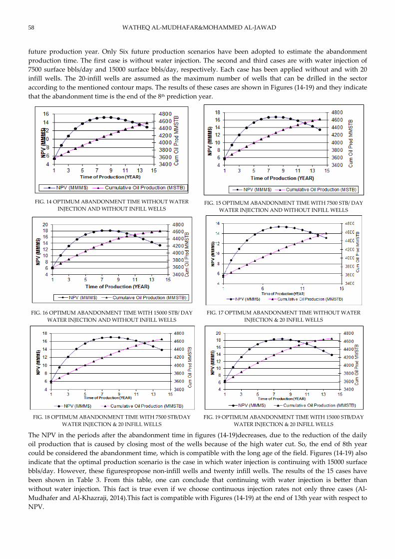
future production year. Only Six future production scenarios have been adopted to estimate the abandonment
production time. The first case is without water injection. The second and third cases are with water injection of
7500 surface bbls/day and 15000 surface bbls/day, respectively. Each case has been applied without and with 20
infill wells. The 20‐infill wells are assumed as the maximum number of wells that can be drilled in the sector
according to the mentioned contour maps. The results of these cases are shown in Figures (14‐19) and they indicate
that the abandonment time is the end of the 8th prediction year.
FIG. 14 OPTIMUM ABANDONMENT TIME WITHOUT WATER
INJECTION AND WITHOUT INFILL WELLS
FIG. 15 OPTIMUM ABANDONMENT TIME WITH 7500 STB/ DAY
WATER INJECTION AND WITHOUT INFILL WELLS
FIG. 16 OPTIMUM ABANDONMENT TIME WITH 15000 STB/ DAY
WATER INJECTION AND WITHOUT INFILL WELLS
FIG. 17 OPTIMUM ABANDONMENT TIME WITHOUT WATER
INJECTION & 20 INFILL WELLS
FIG. 18 OPTIMUM ABANDONMENT TIME WITH 7500 STB/DAY
WATER INJECTION & 20 INFILL WELLS
FIG. 19 OPTIMUM ABANDONMENT TIME WITH 15000 STB/DAY
WATER INJECTION & 20 INFILL WELLS
The NPV in the periods after the abandonment time in figures (14‐19)decreases, due to the reduction of the daily
oil production that is caused by closing most of the wells because of the high water cut. So, the end of 8th year
could be considered the abandonment time, which is compatible with the long age of the field. Figures (14‐19) also
indicate that the optimal production scenario is the case in which water injection is continuing with 15000 surface
bbls/day. However, these figurespropose non‐infill wells and twenty infill wells. The results of the 15 cases have
been shown in Table 3. From this table, one can conclude that continuing with water injection is better than
without water injection. This fact is true even if we choose continuous injection rates not only three cases (Al‐
Mudhafer and Al‐Khazraji, 2014).This fact is compatible with Figures (14‐19) at the end of 13th year with respect to
NPV.

Optimization of Infill OilWell Locations 59
Prediction of Optimal Number & Locations of Wells
Table 3 shows that the case2 & case3 of water injection are better than case1, which is without water injection.
Therefore, it is clear that having continuing water injection for the future production is better than no injection to
increase the oil production as well as the net present value. The two cases were investigated in more details for
optimizations of infill oil wells.
In case 3, all the future reservoir evaluation scenarios consist of injecting 15,000 surface bbls of water a day per
injector. 20 simulation runs have been made according to the number of suggested producers from 1 to 20 new
wells in additive way. The locations of these wells are chosen with the aid of the contour maps presented in
Figures (4‐13). The NPV calculation results of the suggested producers are shown in Fig. 20 that indicate that the
optimal number of wells when running the simulator to the end of 8th year (abandonment time) is 19 wells, as
shown in Figure 20. However, that result may not be applicable because it was suggested that drilling the
suggested wells should be completed in the year prior to the 1st year. In addition, the current surface facilities
related to the water injection operations cannot handle this amount of water in addition to the limited amounts of
waters in the recent years in the mentioned area.
Therefore,the choice of three wells is more reasonable since its NPV does not differ very much from that of 19 wells
as shown in Fig. 20. The difference in NPV between the two cases is 0.054377% only.
In the other hand, case2 suggests injection 7500 surface bbls of water eachday per well. Similar to case 3, the
locations of the additive 20 suggested oil wells were proposed according to the contour maps of permeability and
oil saturation.
TABLE 3 NPV RESULTS FOR DIFFERENT FUTURE PREDICTION RUNS AT THE END OF 8TH YEAR
Cases # Infill wells Well Injection Rate (surface bbls/day) Cum. Oil Production (MMSTB) RF (%) NPV, MMM $
1
0 0 4172.089 59.974 15.20525
5 0 4178.827 60.071 15.3279
10 0 4178.235 60.062 15.30102
15 0 4179.956 60.087 15.32594
20 0 4181.181 60.105 15.34154
2
0 7500 4262.067 61.268 16.82088
5 7500 4271.293 61.400 16.99321
10 7500 4270.649 61.391 16.96579
15 7500 4272.533 61.418 16.99403
20 7500 4273.380 61.430 17.00113
3
0 15000 4336.217 62.333 18.11828
5 15000 4349.621 62.526 18.37543
10 15000 4350.236 62.535 18.37405
15 15000 4351.874 62.559 18.39648
20 15000 4352.292 62.565 18.39488
FIG. 20 OPTIMAL NUMBER OF WELLS WITH 15000 SURFACE
BBL/DAY AT THE END OF 8TH YEAR
FIG. 21 OPTIMAL NUMBER OF WELLS WITH 7500 SURFACE
BBL/DAY AT THE END OF 8TH YEAR
18.1
18.15
18.2
18.25
18.3
18.35
18.4
18.45
0 5 10 15 20 25
No. of Proposed Wells
NP
V (
MM
M$)
43344336433843404342434443464348435043524354
Cu
mu
lati
ve O
il
Pro
du
ctio
n (
MS
TB
)
NPV (MMM$) Cumulative Oil Production (MSTB)
16.8
16.85
16.9
16.95
17
17.05
0 2 4 6 8 10 12 14 16 18 20 22
No. of Proposed Wells
NP
V,
MM
M$
4.260
4.262
4.264
4.266
4.268
4.270
4.272
4.274
Cu
mu
lati
ve O
il
Pro
du
ctio
n,
MM
MS
TB
NPV, MMM$ Cumulative Oil Production, MMMSTB
60 WATHEQ AL‐MUDHAFAR&MOHAMMED AL‐JAWAD
The optimal number of wells is only three wells, as they achieve the highest NPV among all other proposednumber
of new producers. In addition, this outcome comes in compatible with the current surface capability of injection
facilities with respect to the water resources and the required pressure. Fig. 21 depicts that the optimal numbers of
infill wells as three wells considering the abandonment time to the end of 8th year with water injection of 7500
surface bbls/day in each injection well.
From Fig. 21, one can notice that the optimal number of infill wells reaches the maximum when considering the
cumulative oil production as objective function. However, increasing the number of suggested producers leads to
increase the drilling costs, and decrease the net present value.
The final optimal number and locations of wells between the two cases of different water injection rates is three
since the NPV is more than any other option.Thesethree wells are the same optimal wells in the same locations that
obtained from case3 and they are located at the western side of the reservoir crest, far away from the aquifer
boundaries.
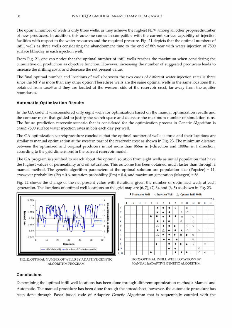
Automatic Optimization Results
In the GA code, it wasconsidered only eight wells for optimization based on the manual optimization results and
the contour maps that guided to justify the search space and decrease the maximum number of simulation runs.
The future prediction reservoir scenario that is considered for the optimization process in Genetic Algorithm is
case2: 7500 surface water injection rates in bbls each day per well.
The GA optimization searchprocedure concludes that the optimal number of wells is three and their locations are
similar to manual optimization at the western part of the reservoir crest as shown in Fig. 23. The minimum distance
between the optimized and original producers is not more than 866m in J‐direction and 1000m in I direction,
according to the grid dimensions in the current reservoir model.
The GA program is specified to search about the optimal solution from eight wells as initial population that have
the highest values of permeability and oil saturation. This outcome has been obtained much faster than through a
manual method. The genetic algorithm parameters at the optimal solution are population size (Popsize) = 11,
crossover probability (Pc) = 0.6, mutation probability (Pm) = 0.4, and maximum generation (Maxgen) = 58.
Fig. 22 shows the change of the net present value with iterations given the number of optimized wells at each
generation. The locations of optimal well locations on the grid map are (6, 7), (7, 6), and (6, 5) as shown in Fig. 23.
FIG. 22 OPTIMAL NUMBER OF WELLS BY ADAPTIVE GENETIC
ALGORITHM PROGRAM
FIG.23 OPTIMAL INFILL WELL LOCATIONS BY
MANUAL&ADAPTIVE GENETIC ALGORITHM
Conclusions
Determining the optimal infill well locations has been done through different optimization methods: Manual and
Automatic. The manual procedure has been done through the spreadsheet; however, the automatic procedure has
been done through Pascal‐based code of Adaptive Genetic Algorithm that is sequentially coupled with the
1.675
1.68
1.685
1.69
1.695
1.7
1.705
0 10 20 30 40 50 60
Iterations
NP
V (
MM
M$)
0
1
2
3
4
5
6
7
Num
ber
of
Opti
miz
ed W
ells
NPV (MMM$) Number of Optimizes wells

Optimization of Infill OilWell Locations 61
reservoir flow simulation. The genetic algorithm was used to accelerate the search about the optimal solution. Use
of the net present value as objective function in the current optimization procedure is foundto be better than using
the cumulative oil production because the net present value depends on the economic analysis for determining the
optimal future reservoir scenario. The optimal number of infill production wells when the water injection rate is
7500 surface bbls/day/injector is three in spite of the higher cumulative oil production upon drilling more than
three wells. All the optimized wells are located at the crest of the reservoir. The optimized wells are far away from
the east and west flanks because the water advance from the edge infinite active aquifer has semi‐completely
invaded these two regions. The incremental percent of NPV based on the optimized infill well location scenario are
improvedby 3.4% higher than the base case on no‐infill wells.
Nomenclatures
GOR Gas‐oil ratio, SCF/STB
Bo Oil formation volume factor, bbl/STB
BHFP Bottom hole flowing pressure, psia
C cost, US $
CAPEX Capital expenditure, US $
FV Future value, US $
I No. of grid blocks in x‐directions
J No. of grid blocks in y‐directions
K No. of grid blocks in z‐directions
NPV Net present value, US $
OPEX Operational expenditure, US $
P Pressure, psia
PV Present value, US $
wc Water cut, %
Δz Layer thickness, m
K Permeability, md
So Oil Saturation, %
SCF Standard Cubic Feet
STB Stock Tank Barrel
bbls barrels
OWC Oil‐Water Contact
Maxgen Maximum number of generations
REFERENCES
[1] Beckner, B. L., and Song, X. ”Field Development Using Simulated Annealing‐Optimal Economic Well
Scheduling and Placement.” Paper SPE 30650 presented at the SPE Annual Technical Conference and
Exhibition, Dallas, TX, Oct. 22‐25, 1995.
[2] Al‐Ansari, R.: “The petroleum Geology of the Upper sandstone Member of the Zubair Formation in the
Rumaila South.” Oilfield Ministry of Oil, Dept. of Reservoirs and Fields Development‐Section of Production
Studies, January 1993.
[3] Kabir, C.S. and et.al. ʺLessons Learned From Energy Models: Iraq’s South Rumaila Case Study.ʺ Paper SPE
105131 presented at the SPE Middle East Oil and Gas Show and Conference, Manama, Bahrain, 11‐14 March
2007.
[4] Bittencourt, A. C., and Horne, R. N. “Reservoir Development and Design Optimization.” Paper SPE 38895
presented at the SPE Annual Technical Conference and Exhibition, San Antonio, TX, October 5‐8, 1997.

62 WATHEQ AL‐MUDHAFAR&MOHAMMED AL‐JAWAD
[5] Güyagüler, B. “Optimization of Well Placement and Assessment of Uncertainty.” PhD diss., Stanford
University, 2002.
[6] Badru, O., and Kabir, C.S. “Well Placement Optimization in Field Development.” Paper SPE 84191 presented
at the SPE Annual Technical Conference and Exhibition, Denver, Colorado, October 5‐8, 2003.
[7] Quenes, A., et al. “A New Method to Characterize Fracture Reservoirs: Application to Infill Drilling.” Paper
SPE 27799 presented at the SPE/DOE Ninth Symposium on Improved Oil Recovery, Tulsa, Oklahoma, April
17‐20, 1994.
[8] Phillips, D., Ravindran, A. and Solberg, J. “Operation Research principle and practice.” John Wiley & Sons
Inc., 1976.
[9] Austin, S. “An Introduction to Genetic algorithm” AI expert. PP 49‐51, 1990.
[10] Al‐Mudhafer, W. J., M. S. Al Jawad, and D. A. Al‐Shamaa.ʺReservoir Flow Simulation Study for a Sector in
Main Pay‐South Rumaila Oil Field.ʺ Paper SPE 126427 presented at the SPE Oil and Gas India Conference and
Exhibition. Mumbai, India, January 20‐22, 2010.
[11] Güyagüler, B. and Horne, R.N. “Optimization of Well Placement.” Paper SPE presented at the ASME Energy
Sources Technology Conference in New Orleans, February 14‐16, 2002.
[12] Ozdogan, U. “Optimization of Well Placement under Time‐Dependent Uncertainty.” MS Thesis, Stanford
University, 2004.
[13] Al‐Mudhafer, W. J., M. S. Al Jawad, and D. A. Al‐Shamaa. “Using Optimization Techniques for Determining
Optimal Locations of Additional Oil Wells in South Rumaila Oil Field.ʺ Paper SPE 130054 presented at the
CPS/SPE International Oil and Gas Conference and Exhibition, Beijing, China, 8–10 June, 2010.
[14] Mian, M.A. “Petroleum Engineering, Handbook for the practicing Engineer.” PennWell Publishing Company,
1992.
[15] Beecroft, W. J., and Shtern, V.N. “Novel Approach to Optimization of Infill Drilling Using Conformance
Mapping Technique.” Paper SPE 56815 presented at the SPE Annual Technical Conference and Exhibition,
Houston, Texas, 3‐6 October 1999.
[16] Al‐Mudhafer, W. J., M. S. Al Jawad, and D. A. Al‐Shamaa. ʺOptimal Field Development through Infill Drilling
for the Main Pay in South Rumaila Oil Field.ʺ Paper SPE 132303 presented at the Trinidad and Tobago Energy
Resources Conference, Port of Spain, Trinidad, 27–30 June, 2010.
[17] Hamdullah, Sameera. “Modelling a Sector of the Main Reservoir of south Rumaila Oil Field.” Ph.D. Diss.,
University of Baghdad, 1999.
[18] Johnston, D. “International exploration Economics, Risk, and Contract Analysis.” PennWell Publishing Co. 19,
2003.
[19] Nwaozo, J. “Dynamic Optimization of a Water Flood Reservoir.” PhD Diss., University of Oklahoma, 2006.
[20] Jefferys, E.R. “Design Application of Genetic Algorithm.” Paper SPE 26367 presented at the 68th SPE Annual
Technical Conference and Exhibition, Houston, Texas, 3‐6 October 1993.
[21] Goldberg, D.E.“Genetic Algorithm in Search, optimization and Machine learning.” Addison‐Wesley, Reading,
MA, 1989.
[22] Mohaghegh, S. “Virtual Intelligence and its Applications in petroleum Engineering’ Part 2. Evolutionary
Computing” Distinguished Author Series, West Virginia University, 2001.
[23] Romero, C.E., Carter, J.N., Zimmerman, R.W., and Gringarten, A.C. “A Modified Genetic Algorithm for
Reservoir Characterization,” paper SPE 64765 presented at the 17th International Oil and Gas Conference and
Exhibition in China, Beijing, China, November 7‐10, 2000.
[24] Mohaghegh, S., Arefi, R., Ameri, S., and Rose, D. “A Methodological Approach For Reservoir Heterogeneity

Optimization of Infill OilWell Locations 63
Characterization Using Artificial Neural Networks.” paper SPE 28394 presented at the SPE Annual Technical
Conference & Exhibition held in New Orleans, LA, U.S.A., September 25‐28, 1994.
[25] Romero, C.E., Carter, J.N., Zimmerman, R.W., and Gringarten, A.C. “Improved Reservoir Characterization
through Evolutionary Computation,” paper SPE 62942 presented 2000 SPE Annual Technical Conference and
Exhibition held in Dallas, Texas, October 1–4, 2000.
[26] Mohaghegh, S., Hill, D., and Reeves, S. “Development of an Intelligent Systems Approach for Restimulation
Candidate Selection.” paper SPE 59767 presented at the Gas Technology Symposium held in Calgary, AB,
Canada, April 3‐5, 2000.
[27] Martinez, E.R. et al. “Application of Genetic Algorithm on the Distribution of Gas‐Lift Injection”, paper SPE
26993 presented at the 69th Annual Technical Conference and Exhibition held in New Orleans, LA, U.S.A.,
September 25‐28, 1994.
[28] Fang, J.H., Karr, C.l. & Stanley, D.A. “Genetic Algorithm and its Application to Petrophysics.” paper SPE
26208 presented at the Annual Technical Conference and Exhibition, Tuscaloosa, Dec.10, 1992.
[29] Yin, Hongjun, Zhai, Yunfang, “An Optimum Method of Early‐Time Well Test Analysis ‐‐ Genetic Algorithm.”
paper SPE 50905 presented at the International Oil & Gas Conference and Exhibition in China held in Beijing,
China, 2‐6 November 1998.
[30] Güyagüler, B. and Horne, R.N. “Automated Reservoir Model Selection in Well Test Interpretation.” paper SPE
71569 presented at the Annual Technical Conference and Exhibition, held in New Orleans, Louisiana, U.S.A.,
September 30 to October 3, 2001.
[31] Mohaghegh, S., Balan, B., Ameri, S., and McVey, D.S. “A Hybrid, Neuro‐Genetic Approach to Hydraulic
Fracture Treatment Design and Optimization.” paper SPE 36602 presented at the Annual Technical
Conference and Exhibition held in Denver, Colorado, October 6‐9, 1996.
[32] Mohaghegh, S., Popa, A. S. and Ameri, S. “Intelligent Systems Can Design Optimum Fracturing Jobs.” paper
SPE 57433 presented at the Eastern Regional Conference and Exhibition, Charleston, West Virginia, October
21‐22, 1999.
[33] Palke, M.R., and Horne, R.N. “Determining the Value of Reservoir Data by Using Nonlinear Production
Optimization Techniques.” paper SPE 38047 presented at the 1997 SPE Asia Pacific Oil & Gas Conference and
Exhibition, held in Kuala Lumpur, Malaysia, April14‐16, 1997.
[34] Sen, M.K. et al. “Stochastic Reservoir Modelling Using Simulated Annealing and Genetic Algorithm.” paper
SPE 24754 presented at the 67th Annual Technical Conference and Exhibition of SPE held in Washington, DC,
October 4‐7, 1992.
[35] Artus, V., Durlofsky, L.J., Aziz, K. “Optimization of Nonconventional Well Deployment using a Genetic
Algorithm.” paper presented at the 12th SUPRI‐HW Industrial Affiliates Meeting Nov 18‐19, 2004.
[36] Mohaghegh, S., Platon, V., and Ameri, S. “Candidate Selection for Stimulation of Gas Storage Wells Using
Available Data With Neural Networks and Genetic Algorithms.” Paper SPE 51080, SPE Eastern Regional
Meeting held in Pittsburgh, PA, November 9‐11, 1988.
[37] Fichter, D. P. “Application of Genetic Algorithms in Portfolio Optimization for the Oil and Gas Industry.”
paper SPE 62970 presented at the SPE Annual Technical Conference and Exhibition, Dallas, Texas, October 1‐
4, 2000.
[38] Bittencourt, A. C. “Optimal Scheduling of Development in an Oil Field,” MS report, Stanford University, 1994.
[39] Guerreiro, J.N.C., et al. “Identification of Reservoir Heterogeneities Using Tracer Breakthrough Profiles and
Genetic Algorithms.” paper SPE 39066 presented at the Latin American and Caribbean Petroleum Engineering
Conference and Exhibition held in Rio de Janeiro, Brazil, August‐30, September‐3, 1997.

64 WATHEQ AL‐MUDHAFAR&MOHAMMED AL‐JAWAD
[40] Al‐Mudhafer, W. J. ʺCoupling Programming of an Adaptive Genetic Algorithm with Reservoir Flow
Simulation for Infill Oil Well Locations Optimization.ʺ paper SPE 165670 presented a at the SPE Western
Regional & AAPG Pacific Section Meeting, 2013 Joint Technical Conference held in Monterey, California, USA
(19‐25 April 2013).
[41] Da. Ruan, “Intelligent Hybrid Systems Fuzzy logic, Neural Networks, and Genetic Algorithms.” Kluwer
Academic Publishers, 1997.
[42] Grant, K. “An Introduction to Genetic algorithm.” C/C++ user Journal, pp 45‐58, 1995.
[43] Mitchell, M. “An Introduction to Genetic algorithm.” A Bradford Book, 1996.
[44] Schmidt, M. and Stiden, T. “Hybrid systems: Genetic Algorithm, Neural Networks, and Fuzzy logic” DAIMI
IR, 1997.
[45] Al‐Mudhafer, W. J., & Al‐Khazraji, A. J. Efficient Reservoir Modeling‐Statistical Approach for Evaluation and
Development of Future Waterdrive Undersaturated Oil Reservoir Performance,ʺ IPTC 18102 presented at the
International Petroleum Technology Conference, Kuala Lumpur, Malaysia (10‐12 December 2014).
Watheq J. Al‐Mudhafaris a PhD candidate at Craft & Hawkins department of Petroleum Engineering at Louisiana State
University and A&M College. He has obtained his B.Sc. and M.Sc. in petroleum engineering from the University of Baghdad,
Baghdad, Iraq. His research interest focus on Geostatistical reservoir characterization, reservoir simulation, optimization, and
Enhanced Oil Recovery.
He has three years experience as field engineer in workover, completion, acidizing, and well logging & three years as senior
reservoir engineer in South Oil Company, Basrah, Iraq.
Mr. Al‐Mudhafar has Fulbright Science & Technology International Award. He has published more than 30 papers related his
research disciples in the last four years.
Mohammed Al‐Jawad is a professor of petroleum engineering at the University of Technology, Baghdad, Iraq. He is the Liaison
of the Ministry of Higher Education in the Ministry of Oil, Iraq. He has B.Sc., M.Sc., and PhD in petroleum engineering from
University of Baghdad, Iraq.
He has more than 28 years experience in education and has published more than 20 papers. His research interests focus on
numerical reservoir simulation, optimization, and PVT modeling.
Dr. Al‐Jawad has supervised more than 30 PhD dissertations and M.Sc. theses during his academic life in the University of
Baghdad and the University of Technology.

Journal of Petroleum Science Research, Vol. 4 No. 2‐July 2015 65
2168‐5517/15/02 065‐14, © 2015 DEStech Publications, Inc.
doi: 10.12783/jpsr.2015.0402.03
The Use of Regression and Classification
Algorithms for Layer Productivity Prediction
in Naturally Fractured Reservoirs Shiyun Mi1, Guangren Shi*2
Research Institute of Petroleum Exploration and Development, PetroChina, P. O. Box 910, Beijing100083, China
[email protected]; *[email protected]
Abstract
Three regression algorithms and three classification algorithms have been applied to forecast naturally fractured layer
productivity. The three regression algorithms are the regression of support vector machine (R‐SVM), the back‐propagation
neural network (BPNN), and the multiple regression analysis (MRA), while the three classification algorithms are the
classification of support vector machine (C‐SVM), the naïve Bayesian (NBAY), and the Bayesian successive discrimination
(BAYSD). In general, when all these six algorithms are used to solve a real‐world problem, they often produce different solution
accuracies. When an algorithm is applied to a real‐world problem, its solution accuracy is expressed with the total mean
absolute relative residual for all samples, R(%). In this paper, three criteria have been proposed: 1) nonlinearity degree of a
studied problem based on R(%) of MRA (weak if R(%)<10, moderate if 10≤R(%)≤30, and strong if R(%)>30); 2) solution accuracy
of a given algorithm application based on its R(%) (high if R(%)<10, moderate if 10≤ R(%)≤30, and low if R(%)>30); and 3) results
availability of a given algorithm application (applicable if R(%)<10, and inapplicable if R(%)≥10). A case study of naturally
fractured layer productivity at an oilfield in Sichuan Province of China has been used to validate the proposed approach. This
case study consists of two problems: regression and classification. For the regression problem, R‐SVM, BPNN and MRA are
inapplicable because their R(%) values are 4620, 44 and 5980, respectively. For the classification problem, however, C‐SVM,
NBAY and BAYSD are all applicable since their R(%) values are 0, 5.9 and 9.1, respectively. From the case study, it is concluded
that: a) the three proposed criteria, and the rules of conversion from real number to integer number are practical; b) R(%) of
MRA is used to measure the nonlinearity degree of a studied problem, and thus MRA should be used as a first choice; c) for
classification problems, the preferable algorithm is C‐SVM, NBAY, or BAYSD if the problems nonlinearity is weak or moderate,
and BAYSD can also serve as a promising dimension‐reduction tool; d) for regression problems, the preferable algorithm is
BPNN, but MRA can serve as a promising dimension‐reduction tool only when the problems are linear; e) if BPNN is
inapplicable for a regression problem, it is proposed to change the problem from regression to classification by reasonable
conversion rules, then apply C‐SVM, NBAY, or BAYSD; and f) comparing with C‐SVM, BAYSD is conditionally better.
Keywords
Problem Nonlinearity; Solution Accuracy; Results Availability; Conversion Rules; Dimensionality Reduction; Naturally Fractured Layer
Productivity; Sichuan Province in China
Introduction
Three regression algorithms and three classification algorithms have been applied to forecast naturally fractured
layer productivity. The three regression algorithms are the regression of support vector machine (R‐SVM), the
back‐propagation neural network (BPNN), and the multiple regression analysis (MRA), while the three
classification algorithms are the classification of support vector machine (C‐SVM), the naïve Bayesian (NBAY), and
the Bayesian successive discrimination (BAYSD). In general, when all these six algorithms are used to solve a real‐
world problem, they often produce different solution accuracies. When an algorithm is applied to a real‐world
problem, its solution accuracy is expressed with the total mean absolute relative residual for all samples, R(%). In
this paper, three criteria have been proposed: a) nonlinearity degree of a studied problem based on R(%) of MRA
(weak if R(%)<10, moderate if 10≤R(%)≤30, and strong if R(%)>30); b) solution accuracy of a given algorithm
application based on its R(%) (high if R(%)<10, moderate if 10≤ R(%)≤30, and low if R(%)>30); and c) results
availability of a given algorithm application (applicable if R(%)<10, and inapplicable if R(%)≥10). A case study of
naturally fractured layer productivity at an oilfield in Sichuan Province of China has been used to validate the
proposed approach.

66 SHIYUN MI, GUANGREN SHI
Methodology
The methodology consists of the following three major parts: definitions commonly used by regression and
classification algorithms; six algorithms; dimensionality reduction.
Definitions Commonly Used by Regression and Classification Algorithms
The aforementioned regression and classification algorithms share the data of samples. The essential difference
between the two types of algorithms is that the output of regression algorithms is real‐type value and in general
differs from the real number given in the corresponding learning sample, whereas the output of classification
algorithms is integer‐type value and must be one of the integers defined in the learning samples. In the view of
dataology, the integer‐type value is called as discrete attribute, while the real‐type value is called as continuous
attribute.
The six algorithms (R‐SVM, BPNN, MRA, C‐SVM, NBAY, BAYSD) use the same known parameters, and also share
the same unknown that is predicted. The only difference between them is the approach and calculation results.
Assume that there are n learning samples, each associated with m+1 numbers (x1, x2, …, xm, y*) and a set of observed
values (xi1, xi2, …, xim, *iy ), with i=1, 2, …, n for these numbers. In principle, n>m, but in actual practice n>>m. The n
samples associated with m+1 numbers are defined as n vectors:
xi=(xi1, xi2, …, xim, *iy ) (i=1, 2, …, n) (1)
where n is the number of learning samples; m is the number of independent variables in samples; xi is the ith
learning sample vector; xij is the value of the jth independent variable in the ith learning sample, j=1, 2, …, m; and *iy
is the observed value of the ith learning sample.
Equation 1 is the expression of learning samples.
Let x0 be the general form of a vector of (xi1, xi2, …, xim). The principles of BPNN, MRA, NBAY and BAYSD are the
same, i.e., try to construct an expression, y=y(x0), such that Eq. (2) is minimized. Certainly, these four different
algorithms use different approaches and obtain calculation results in differing accuracies.
2
*0
1i i
n
iy y
x (2)
where y=y(x0i) is the calculation result of the dependent variable in the ith learning sample; and the other symbols
have been defined in Eq. (1).
However, the principles of R‐SVM and C‐SVM algorithms are to try to construct an expression, y=y(x0), such that to
maximize the margin based on support vector points so as to obtain the optimal separating line.
This y=y(x0) is called the fitting formula obtained in the learning process. The fitting formulas of different
algorithms are different. In this paper, y is defined as a single variable.
The flowchart is as follows: the 1st step is the learning process, using n learning samples to obtain a fitting formula;
the 2nd step is the learning validation, substituting n learning samples (xi1, xi2, …, xim) into the fitting formula to get
prediction values (y1, y2, …, yn), respectively, so as to verify the fitness of an algorithm; and the 3rd step is the
prediction process, substituting k prediction samples expressed with Eq. (3) into the fitting formula to get
prediction values (yn+1, yn+2, …, yn+k), respectively.
xi=(xi1, xi2, …, xim) (i=n+1, n+2, …, n+k) (3)
where k is the number of prediction samples; xi is the ith prediction sample vector; and the other symbols have been
defined in Eq. (1).
Equation 3 is the expression of prediction samples.
In the six algorithms, only MRA is a linear algorithm whereas the other five are nonlinear algorithms, this is due to
the fact that MRA constructs a linear function whereas the other five construct nonlinear functions, respectively.

The Use of Regression and Classification Algorithms for Layer Productivity Prediction in Naturally Fractured Reservoirs 67
To express the calculation accuracies of the prediction variable y for learning and prediction samples when the six
algorithms are used, the following four types of residuals are defined.
The absolute relative residual for each sample, R(%)i (i=1, 2, …, n, n+1, n+2, …, n+k), is defined as
* *(%) ( ) / 100i i iiR y y y = - (4)
where yi is the calculation result of the dependent variable in the ith sample; and the other symbols have been
defined in Eqs. (1) and (3). R(%)i is the fitting residual to express the fitness for a sample in learning or prediction
process.
It is noted that zero must not be taken as a value of *iy to avoid floating‐point overflow. Therefore, for regression
algorithm, delete the sample if its *iy =0; and for classification algorithm, positive integer is taken as values of *
iy .
The mean absolute relative residual for all learning samples, R1(%), is defined as
1 1(%) /i
n
iR R n
(%)= (5)
where all symbols have been defined in Eqs. (1) and (4). R1(%) is the fitting residual to express the fitness of
learning process.
The mean absolute relative residual for all prediction samples, R2(%), is defined as
2 1(%) /i
k
i nR R k
(%)= (6)
where all symbols have been defined in Eqs. (3) and (4). R2(%) is the fitting residual to express the fitness of
prediction process.
The total mean absolute relative residual for all samples, R(%), is defined as
1(%) (%) / ( )i
n k
iR R n k
= (7)
where all symbols have been defined in Eqs. (1), (3) and (4). If there are no prediction samples, k=0, then
R(%)=R1(%).
R(%) is the fitting residual to express the fitness of learning and prediction processes.
When the six algorithms (R‐SVM, BPNN, MRA, C‐SVM, NBAY, BAYSD) are used to solve a real‐world problem,
they often produce different solution accuracies. Toward this issue, the following three criteria have been proposed
(Table 1).
TABLE 1 CRITERION 1 (NONLINEARITY DEGREE OF A STUDIED PROBLEM), CRITERION 2 (SOLUTION ACCURACY OF A GIVEN ALGORITHM APPLICATION),
AND CRITERION 3 (RESULTS AVAILABILITY OF A GIVEN ALGORITHM APPLICATION)
Range of R(%)
Criterion 1 (nonlinearity degree of a
studied problem) based on R(%) of
MRA
Criterion 2 (solution accuracy of a given
algorithm application) based on its R(%)
Criterion 3 (Results availability of
a given algorithm application)
R(%)<10 Weak High Applicable
10≤R(%)≤30 Moderate Moderate Inapplicable
R(%)>30 Strong Low Inapplicable
Criterion 1: Nonlinearity Degree of a Studied Problem
Since MRA is a linear algorithm, its R(%) for a studied problem expresses the nonlinearity degree of y=y(x) to be
solved, i.e. the nonlinearity degree of the studied problem. This nonlinearity degree can be divided into three
classes: weak, moderate, and strong (Table 1).
Criterion 2: Solution Accuracy of a Given Algorithm Application
Whether linear algorithm (MRA) or nonlinear algorithms (R‐SVM, BPNN, C‐SVM, NBAY, BAYSD), the R(%) value
of a given application expresses the accuracy of y=y(x) obtained by each algorithm, i.e. solution accuracy of each

68 SHIYUN MI, GUANGREN SHI
algorithm for solving the application. This solution accuracy can be divided into three classes: high, moderate, and
low (Table 1).
Criterion 3: Results Availability of a Given Algorithm Application
In general, this results availability is divided into two classes: applicable if R(%)<5, and inapplicable if R(%)≥5. In
this paper, however, this results availability is divided into two classes: applicable if R(%)<10, and inapplicable if
R(%)≥10 (Table 1). This is because the subsurface geoscience is different from the other fields, with miscellaneous
data types, huge quantity, different measuring precision, and lots of uncertainties to data processing results (Shi,
2013).
Six Algorithms
Through the learning process, each method constructs its own function y=y(x). The methods of the six methods (R‐
SVM, BPNN, MRA, C‐SVM, NBAY, BAYSD) are described below. It is noted that y=y(x) created by BPNN is an
implicit expression, i.e. which cannot be expressed as a usual mathematical formula; whereas that of the other five
methods are explicit expressions, i.e. which are expressed as a usual mathematical formula.
The following will discuss the six methods. Because support vector machine (SVM) has both classification (C‐SVM)
and regression (R‐SVM) methods, SVM is generally introduced ahead. Since the 1990ʹs, SVM has been gradually
applied in natural and social sciences, especially widely in this century. SVM is an approach utilizing machine‐
learning based on statistical learning theory. It is essentially performed by converting a real‐world problem (the
original space) into a new higher dimensional feature space using the kernel function, and then constructing a
linear discriminate function in the new space to replace the nonlinear discriminate function. Theoretically, SVM
can obtain the global optimal solution and avoid converging to a local optimal solution as can possibly occur in
BPNN, though this problem in BPNN is rare if BPNN is properly coded (Shi, 2013). The SVM procedure includes
two principal methods: 1) C‐SVM, such as the binary classification (Shi, 2013, 2009; Shi and Yang, 2010; Chang and
Lin, 2011; Shi et al., 2014), and the ‐binary classification (Chang and Lin, 2001); and 2) R‐SVM, such as the ‐regression (Shi, 2013; Chang and Lin, 2011; Shi et al., 2014), and the ‐regression (Chang and Lin, 2002). In the case study below, the binary classification for C‐SVM and the ‐regression for R‐SVM are employed. Moreover, it is
better to take RBF (radial basis function) as a kernel function than to take the linear, polynomial and sigmoid
functions under strong nonlinear conditions (Shi, 2013; Chang and Lin, 2011), and thus the kernel function used in
C‐SVM and R‐SVM is the RBF.
1) R‐SVM
A technique of R‐SVM, ‐regression (Shi, 2013; Chang and Lin, 2011), has been employed. The formula created
by this technique is an expression with respect to a vector x, which is so‐called a nonlinear function y=R‐SVM(x1,
x2, …, xm):
* 2
1( ) exp( || || )
ni iii
y b x x (8)
where α and α* are the vector of Lagrange multipliers, α=(α1, α2, …, αn) and α*=( *1
, *2
, …, *n
), 0≤αi≤C and
0≤ *i ≤C where C is the penalty factor, and the constraint *
1( )
niii
=0; 2exp( || || )i x x is a RBF kernel
function; γ is the regularization parameter, γ>0; and b is the offset of the separating hyperplane, which can be
calculated using the free vectors xi. These free xi are those vectors corresponding to αi>0 and *i >0, on which the
final R‐SVM model depends.
αi, *i , C, and γ can be solved using the dual quadratic optimization:
* *
*
* * 2
1 1,
), 1
max ( ) ( )
1 ( )( exp( || || )2
n ni i i i i
i i
ni i j j i j
i j
y
α α
x x
(9)

The Use of Regression and Classification Algorithms for Layer Productivity Prediction in Naturally Fractured Reservoirs 69
where (>0) is determined by user.
It is noted that in the case study below the formulas corresponding to Eq. (8) are not concretely written out due
to their large size.
2) BPNN
The BPNN procedure has been widely applied since the 1980ʹs (Shi, 2013; Darabi et al., 2010; Labani et al., 2010),
and the application of BPNN is still predominant. The formula created by BPNN is an expression with respect
to m parameters (x1, x2, …, xm) (Shi, 2013):
y=BPNN(x1, x2, …, xm) (10)
where BPNN is a nonlinear function, which cannot be expressed as a usual mathematical formula and so it is an
implicit expression. BPNN consists of one input layer, one or more hidden layers, and one output layer. In the
case study below, only one hidden layer is employed. There is no theory yet to determine how many hidden
layers are needed for any given case, but in the case of output layer with only one node, it is enough to define
one hidden layer. Moreover, it is also difficult to determine how many nodes a hidden layer should have. For
solving local minima problem, it is suggested to use the large Nhidden=2(Ninput+Noutput)−1 estimate where Nhidden is
the number of hidden nodes, Ninput is the number of input nodes and Noutput is the number of output nodes. The
values of the network learning rate for the output layer and the hidden layer are within (0, 1), and in practice
they can be the same.
The term back‐propagation refers to the way (Shi, 2013; Güler and Übeyli, 2003), the error computed at the
output side is propagated backward from the output layer, to the hidden layer, and finally to the input layer.
Each iteration of BPNN constitutes two sweeps: forward to calculate a solution by using a sigmoid activation
function, and backward to compute the error and thus to adjust the weights and thresholds for the next
iteration. This iteration is performed repeatedly until the solution agrees with the desired value within a
required tolerance. The error takes the root mean square error (Shi, 2013; Hush and Horne, 1993) is
RMSE(%)= * 21
1( )
n
i in iy y
×100 (11)
where yi and *iy are under the conditions of normalizations in the learning process. RMSE(%) is used in the
conditions for terminating network learning.
3) MRA
The MRA procedure has been widely applied since the 1970ʹs (Shi, 2013; Sharma et al., 2010; Singh et al., 2008),
and the successive regression analysis, the most popular MRA technique, is still a very useful tool. The formula
created by this technique is a linear combination with respect to m parameters (x1, x2, …, xm), plus a constant
term, which is so‐called a linear function y=MRA(x1, x2, …, xm) (Shi, 2013):
y=b0+b1x1+b2x2+…+bmxm (12)
where the constants b0, b1, b2, …, bm are deduced using regression criteria and calculated by the successive
regression analysis of MRA. Eq. (12) is a so‐called “regression equation”. In rare cases an introduced xk can be
deleted in the regression equation, and in much rarer cases a deleted xk could be again introduced into the
regression equation. Therefore, usually Eq. (12) is solved via m iterations.
4) C‐SVM
A technique of C‐SVM, the binary classifier (Shi, 2013; Chang and Lin, 2011), has been employed. The formula
created by this technique is an expression with respect to a vector x, which is so‐called a nonlinear function y=C‐
SVM(x1, x2, …, xm):
2
1exp( || || )
ni i i
iy y b
x x (13)
where α is the vector of Lagrange multipliers, α=(α1, α2, …, αn), 0≤αi≤C where C is the penalty factor, and the

70 SHIYUN MI, GUANGREN SHI
constraint 1
ni i
iy
=0; 2exp( || || )i x x is a RBF kernel function; γ is the regularization parameter, γ>0; and b is
the offset of the separating hyperplane, which can be calculated using the free vectors xi. These free xi are those
vectors corresponding to αi>0, on which the final C‐SVM model depends.
αi, C, and γ can be solved using the dual quadratic optimization:
2
1 , 1
1max exp( || || )
2
n ni i j i j i j
i i jy y
αx x (14)
It is noted that in the case study below the formulas corresponding to Eq. (13) are not concretely written out due
to their large size.
5) NBAY
The NBAY procedure has been widely applied since the 1990ʹs, and widely applied in this century (Shi, 2013;
Ramoni and Sebastiani, 2001). The following introduces a NBAY technique, i.e. the naïve Bayesian. The formula
created by this technique is a set of nonlinear products with respect to m parameters (x1, x2, …, xm) (Shi, 2013;
Tan et al., 2005; Han and Kamber, 2006):
2
21
( )1
2 2( ) exp
( 1,2,..., )
j jl
jl jl
ml j
xN
l L
x (15)
where l is the class number, L is the number of classes, Nl(x) is the discrimination function of the lth class with
respect to x, σjl is the mean square error of xj in Class l, μjl is the mean of xj in Class l. Eq. (15) is so‐called a naïve
Bayesian discrimination function.
Once Eq. (15) is created, any sample shown by Eq. (1) or Eq. (3) can be substituted in Eq. (15) to obtain L values:
N1, N2, …, NL. If b 1
max lll L
N N
, then
y=lb (16)
for this sample.
Eq. (16) is so‐called a nonlinear function y=NBAY (x1, x2, …, xm).
6) BAYSD
The BAYSD procedure has been widely applied since the 1990ʹs, and widely applied in this century (Shi, 2013;
Denison et al., 2002; Shi, 2011). The following introduces BAYSD technique. The formula created by this
technique is a set of nonlinear combinations with respect to m parameters (x1, x2, …, xm), plus two constant terms
(Shi, 2013):
01
( ) ln( ) ( 1, 2,... )m
jl l l jlj
B p c c x l L
x (17)
where l is the class number, L is the number of classes, Bl(x) is the discrimination function of the lth class with
respect to x, cjl is the coefficient of xj in the lth discrimination function, pl and c0l are two constant terms in the lth
discrimination function. The constants pl, c0l, c1l, c2l, …, cml are deduced using Bayesian theorem and calculated by
the successive Bayesian discrimination. Eq. (17) is so‐called a Bayesian discrimination function. In rare cases an
introduced xk can be deleted in the Bayesian discrimination function, and in much rarer cases a deleted xk could
be again introduced into the Bayesian discrimination function. Therefore, usually Eq. (17) is solved via m
iterations.
Once Eq. (17) is created, any sample shown by Eq. (1) or Eq. (3) can be substituted in Eq. (17) to obtain L values:
B1, B2, …, BL. If b 1
max lll L
B B
, then

The Use of Regression and Classification Algorithms for Layer Productivity Prediction in Naturally Fractured Reservoirs 71
y=lb (18)
for this sample.
Eq. (18) is so‐called a nonlinear function y=BAYSD(x1, x2, …, xm).
In the case study below, for both R‐SVM and C‐SVM, the termination of calculation accuracy TCA is fixed to
0.001, and the RBF is taken as a kernel function.
Dimensionality Reduction
The definition of dimensionality reduction is to reduce the number of dimensions of a data space as small as
possible but the results of studied problem are unchanged. The benefits of dimensionality reduction are to reduce
the amount of data can enhance the calculating speed, to reduce the independent variables can extend applying
ranges, and to reduce misclassification ratio of prediction samples can enhance processing quality.
Among the aforementioned six algorithms, each of MRA and BAYSD can serve as a promising dimension‐
reduction tool, respectively, because the two algorithms all can give the dependence of the predicted value (y) on
independent variables (x1, x2, …, xm), in decreasing order. However, because MRA belongs to data analysis in linear
correlation whereas BAYSD is in nonlinear correlation, in applications the preferable tool is BAYSD, whereas MRA
is available only when the studied problems are linear. The called “promising tool” means whether it succeeds or
not that needs a high‐class nonlinear tool (e.g., BPNN for regression problem, C‐SVM for classification problem) for
the validation, so as to determine how many independent variables can be reduced.
For example, a case study (Shi et al., 2014) is a 16‐D problem (x1, x2, …, x15, y). For MRA, x1 is the minimum
dependence of y, so we tried to delete x1 and run C‐SVM, the results show R1(%)=0.036 and R2(%)=8.13, but the
results without this deletion are R1(%)=0 and R2(%)=6.30, which indicates this dimension‐reduction fails. For
BAYSD, however, it runs in the condition without x13, x7, x6, x14 x12, x3, x2 and x9, its R(%) is 16.81 that is the same as
that without this deletion, which shows the dimension of this studied problem can be reduced from 16‐D to 8‐D.
Why is the dimension‐reduction of BAYSD succeeded but that of MRA failed? The reason is that the nonlinearity of
the studied problem is strong due to R(%) of MRA is 52.14, and BAYSD is a nonlinear algorithm while MRA is a
linear algorithm.
In the case study below, for the regression problem, dimension‐reduction failed by using MRA and BPNN, i.e., the
13‐D problem (x1, x2, …, x11, x12, y) cannot become 12‐D problem (x1, x2, …, x11, y); for the classification problem,
dimension‐reduction failed by using BAYSD and C‐SVM, i.e., the 13‐D problem (x1, x2, …, x11, x12, y) cannot become
12‐D problem (x2, …, x11, x12, y). That means the expression of variable (y) needs all of 12 independent variables (x1,
x2, …, x12) for this regression problem or this classification problem.
Case Study: Naturally Fractured Layer Productivity at an Oilfield in Sichuan Province of China
This case study consists of two problems: regression and classification. The objective of this case study is to
calculate the natrual productivity of layer (NPL), and to determine the layer productivity classification (LPC) for
naturally fractured layers, which has practical value when well test is less limited.
Using data of 31 samples from an oilfield in Sichuan Province of China, and each sample contains 12 independent
variables (x1 = layer thickness, x2 = morphology type, x3 = maximum of acoustic log, x4 = mimimum of fracture
width, x5 = porosity of fractures, x6 = permeability of fractures, x7 = x6•x1, x8 = fracture density, x9 = absolute
difference of deep laterolog and shallow laterolog, x10 = well logging porosity, x11 = rock porosity, x12 = 10‐2 x11•x1)
and one variable (y* = NPL) given in Table 2, Tang et al. (2008) adopted MRA for the prediction of NPL. In the case
study, among these 31 samples, 28 are taken as learning samples and 3 as prediction samples (Table 2) for the
prediction of both NPL and LPC, in which for NPL using R‐SVM, BPNN and MRA, and for LPC using C‐SVM,
NBAY and BAYSD. It is noted that this LPC is figured out from NPL by using the conversion rules given in Table
3.

72 SHIYUN MI, GUANGREN SHI
TABLE 2 INPUT DATA FOR NATURALLY FRACTURED LAYER PRODUCTIVITY AT AN OILFIELD IN SICHUAN PROVINCE OF CHINA [MODIFIED FROM (TANG ET
AL., 2008)]
Sample
type
Sample
No.
Well
No.
Layer
No.
12 parameters related to ya
y*
x1
(m)
Parameters of
acoustic log
Parameters of
well logging in fractures Parameters of reservoir
x2 x3
(μs/m)
x4
(m)
x5
(%)
x6
(10‐3m2)
x7
(10‐3m2∙m)x8
x9
(Ω∙m)
x10
(%)
x11
(%)
x12
(m) NPLb LPCc
Learning
samples
1 CX1 B 35 2.5 112.56 0.298 0.038 0.14 4.907 0.125 8 8 8.648 3.027 0.001 3
2 CX2 B 18 2 120.62 0.408 0.032 0.223 4.014 0.193 1 11 9.871 1.777 0.001 3
3 CX2 C 13 2.5 111.25 0.963 0.067 2.587 33.63 1.47 5 10 9.463 1.23 1.3163 1
4 CX3 A 24 2 169.06 0.597 0.02 0.293 6.874 0.91 8 9 9.056 2.128 0.1513 2
5 CX3 B 19 2.5 140.94 0.559 0.026 0.335 6.19 0.178 6 11 9.871 1.826 0.5039 2
6 CX3 C 20 3 164.32 0.948 0.169 6.307 126.1 25.9 10 13 10.69 2.137 3.1 1
7 CX4 A 18 2 133.85 0.186 0.027 0.039 0.696 0.61 8 12 10.28 1.85 0.4209 2
8 CX4 C 16 2.5 126.15 0.916 0.079 2.76 42.78 3.06 4 16 11.91 1.846 1.834 1
9 CX5 C 13 2 20 0.152 0.048 0.046 0.601 1.81 1 10 9.463 1.23 0.0054 3
10 CX6 A 25 2.5 180 0.289 0.032 0.111 2.775 0.41 7 9 9.056 2.264 0.62 2
11 CX6 B 26 1 205 0.282 0.03 0.099 2.579 0.286 2 8 8.648 2.248 0.1595 2
12 CX6 C 11 1 170 0.315 0.034 0.136 1.572 0.214 3 10 9.463 1.079 0.1595 3
13 CX7 B 19 2 153.18 0.423 0.04 0.298 5.775 0.08 3 10 9.463 1.836 0.001 3
14 CX7 C 11 2 137.06 0.403 0.044 0.297 3.123 0.11 1 10 9.463 0.994 0.001 3
15 CX8 A 24 3 159.06 0.351 0.077 0.395 9.48 2.31 5 12 10.28 2.467 0.7244 2
16 CX8 B 15 2 16.86 0.237 0.046 0.106 1.619 0.207 5 7 8.24 1.236 0.001 3
17 CX8 C 15 2 149.69 0.306 0.043 0.166 2.487 0.154 5 8.5 8.852 1.328 0.001 3
18 CX9 A 24 4 162.04 0.902 0.067 2.944 70.66 5.45 6 11 9.871 2.369 1.4735 1
19 X1 B 34 2 124.01 0.108 0.059 0.029 0.974 0.092 4 8 8.648 2.94 0.001 3
20 X1 C 14 2 134.26 0.099 0.053 0.022 0.31 0.643 4 11 9.871 1.402 0.515 2
21 X2 B 17 2 142.09 0.335 0.012 0.054 0.915 0.233 2 9 9.056 1.539 0.001 3
22 X2 C 17 3 147.52 0.988 0.123 4.996 84.93 19.9 2 10 9.463 1.609 2.652 1
23 X3 A 17 2 137.41 0.356 0.096 0.507 8.511 1.14 2 13 10.69 1.795 0.856 2
24 X3 B 28 2.5 117.24 0.283 0.036 0.12 3.297 0.196 1 7 8.24 2.266 0.001 3
25 X3 C 8.5 1 86.94 0.328 0.033 0.148 1.255 0.309 0 8 8.648 0.735 0.001 3
26 X4 C 17 3 157.62 1.055 0.127 5.875 99.88 33.85 2 12 10.28 1.747 2.111 1
27 X5 B 37 1.5 127.31 0.123 0.048 0.03 1.113 0.177 2 11 9.871 3.652 0.001 3
28 X8 A 21 1 142.47 0.168 0.022 0.025 0.527 0.178 1 8 8.648 1.816 0.0507 3
Prediction
samples
29 CX1 C 20 2 125.6 0.892 0.08 2.648 52.96 3.25 6 12 10.28 2.056 (1.62) (1)
30 X5 A 21 2 142.27 0.335 0.044 0.205 4.203 0.369 3 13 10.69 2.191 (0.571) (2)
31 X5 C 10 2 132.36 0.191 0.043 0.065 0.654 0.183 2 10 9.463 0.946 (0.001) (3)
a x1 = layer thickness h, x2 = morphology type, x3 = maximum of acoustic log, x4 = mimimum of fracture width, x5 = porosity of fractures, x6 =
permeability of fractures, x7 = x6•x1, x8 = fracture density (number of fractures per meter), x9 = absolute difference of deep laterolog and shallow
laterolog, x10 = well logging porosity, x11 = rock porosity, x12 = 10‐2 x11•x1. b NPL = the natrual productivity of layer (104m3/d) determined by the well test, number in parenthesis is not input data, but is used for
calculating R(%)i.
c LPC = the layer productivity classification (1–high‐productivity layer, 2–intermediate‐productivity layer, 3–low‐productivity layer) determined
by Table3, number in parenthesis is not input data, but is used for calculating R(%)i.
TABLE 3 LAYER PRODUCTIVITY CLASSIFICATION BASED ON NATRUAL PRODUCTIVITY OF LAYER AT AN OILFIELD IN SICHUAN PROVINCE OF CHINA
Layer productivity NPL (Natrual productivity of layer)
(104m3/d) LPC (Layer productivity classification)
High‐productivity layer NPL>1 1
Intermediate‐productivity layer 0.1≤NPL≤1 2
Low‐productivity layer NPL<0.1 3
Regression Problem for Calculating the Natrual Productivity of Layer (NPL)
Using the 28 learning samples with y*= NPL (Table 2) and by R‐SVM, BPNN and MRA, the following three
functions of NPL (y) with respect to 12 independent variables (x1, x2, …, x12) have been constructed.
Using R‐SVM, the result is an explicit nonlinear function corresponding to Eq. (8):
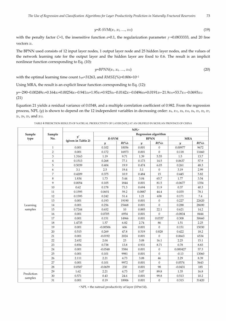
The Use of Regression and Classification Algorithms for Layer Productivity Prediction in Naturally Fractured Reservoirs 73
y=R‐SVM(x1, x2, …, x12) (19)
with the penalty factor C=1, the insensitive function =0.1, the regularization parameter =0.0833333, and 20 free vectors xi.
The BPNN used consists of 12 input layer nodes, 1 output layer node and 25 hidden layer nodes, and the values of
the network learning rate for the output layer and the hidden layer are fixed to 0.6. The result is an implicit
nonlinear function corresponding to Eq. (10):
y=BPNN(x1, x2, …, x12) (20)
with the optimal learning time count topt=31263, and RMSE(%)=0.806×10⁻²
Using MRA, the result is an explicit linear function corresponding to Eq. (12):
y=−290−0.00249x1+0.164x2+0.00254x3−0.941x4+1.95x5+0.925x6−0.0142x7−0.0496x8+0.0191x9−21.9x10+53.7x11−0.0693x12
(21)
Equation 21 yields a residual variance of 0.0348, and a multiple correlation coefficient of 0.982. From the regression
process, NPL (y) is shown to depend on the 12 independent variables in decreasing order: x6, x11, x8, x10, x4, x3, x2, x7,
x1, x9, x5, and x12.
TABLE 4 PREDICTION RESULTS OF NATRUAL PRODUCTIVITY OF LAYER (NPL) AT AN OILFIELD IN SICHUAN PROVINCE OF CHINA
Sample
type
Sample
No.
NPLa
y*
(given in Table 2)
Regression algorithm
R‐SVM BPNN MRA
y R(%)i y R(%)i y R(%)i
Learning
samples
1 0.001 0.102 10056 0.001 0 0.00977 9672
2 0.001 0.172 16973 0.001 0 0.118 11660
3 1.3163 1.19 9.71 1.39 5.55 1.5 13.7
4 0.1513 0.268 77.1 0.173 14.5 0.0637 57.9
5 0.5039 0.404 19.9 0.474 6.03 0.261 48.3
6 3.1 2.5 19.4 3.1 0 3.19 2.99
7 0.4209 0.375 10.9 0.484 15 0.445 5.82
8 1.834 1.73 5.44 3.04 65.7 1.77 3.54
9 0.0054 0.105 1844 0.001 81.5 ‐0.0677 1354
10 0.62 0.178 71.3 0.694 11.9 0.37 40.3
11 0.1595 0.0651 59.2 0.0887 44.4 0.035 78.1
12 0.1595 0.242 51.4 1.21 658 0.171 7.4
13 0.001 0.193 19190 0.001 0 0.227 22620
14 0.001 0.256 25468 0.001 0 0.288 28690
15 0.7244 0.652 10 0.885 22.1 0.621 14.2
16 0.001 0.0705 6954 0.001 0 ‐0.0834 8444
17 0.001 0.151 14966 0.001 0.0337 0.308 30660
18 1.4735 1.57 6.82 2.74 86 1.51 2.25
19 0.001 ‐0.00506 606 0.001 0 0.151 15030
20 0.515 0.269 47.8 0.519 0.828 0.422 18.2
21 0.001 ‐0.0192 2024 0.001 0 0.0663 6534
22 2.652 2.04 23 3.08 16.1 2.25 15.1
23 0.856 0.738 13.8 0.931 8.71 0.78 8.83
24 0.001 ‐0.0548 5584 0.001 0 0.000427 57.3
25 0.001 0.101 9981 0.001 0 ‐0.13 13060
26 2.111 2.21 4.73 3.08 46 2.29 8.39
27 0.001 0.101 9972 0.001 0 0.0574 5643
28 0.0507 ‐0.0659 230 0.001 98 ‐0.0431 185
Prediction
samples
29 1.62 2.21 4.73 3.07 89.8 1.35 16.8
30 0.571 0.43 24.6 0.001 99.8 0.513 10.2
31 0.001 0.19 18906 0.001 0 0.315 31420
a NPL = the natrual productivity of layer (104m3/d).

74 SHIYUN MI, GUANGREN SHI
TABLE 5 COMPARISON AMONG THE APPLICATIONS OF REGRESSION ALGORITHMS (R‐SVM, BPNN AND MRA) TO NATRUAL PRODUCTIVITY OF LAYER (NPL)
AT AN OILFIELD IN SICHUAN PROVINCE OF CHINA
Algorithm Fitting
formula
Mean absolute relative
residual
Dependence of the
predicted value (y)
on independent
variables (x1, x2, …,
x12), in decreasing
order
Time
consuming on
PC (Intel Core
2)
Problem
nonlinearit
y
Solution
accuracy
Results
availabilityR1(%) R2(%) R(%)
R‐SVM Nonlinear,
explicit 4439 6312 4620 N/A 3 s N/A Low Inapplicable
BPNN Nonlinear,
implicit 42 63 44 N/A 30 s N/A Low Inapplicable
MRA Linear,
explicit 5498 10480 5980
x6, x11, x8, x10, x4, x3, x2,
x7, x1, x9, x5, x12 <1 s Strong Low Inapplicable
Substituting the values of 12 independent variables (x1, x2, …, x12) given by the 28 learning samples and 3
prediction sample (Table 2) in Eqs. (19), (20) and (21), respectively, the NPL (y) of each sample is obtained (Table 4).
From Table 5, R‐SVM, BPNN and MRA are inapplicable since their R(%) values are 4620, 44 and 5980, respectively.
Dimension‐Reduction Failed by Using MRA and BPNN
MRA gives the dependence of the predicted value (y) on 12 independent variables, in decreasing order: x6, x11, x8,
x10, x4, x3, x2, x7, x1, x9, x5, x12 (Table 5). According to this dependence order, at first, deleting x12 and running BPNN, it
is found the results of BPNN are changed with R(%)=58 which is greater than previous R(%)=44 (Table 5). Thus the
13‐D problem (x1, x2, …, x11, x12, y) cannot become 12‐D problem (x1, x2, …, x11, y). That means the expression of
variable (y) needs all of 12 independent variables (x1, x2, …, x12) for this regression problem.
Classification Problem for Determining the Layer Productivity Classification (LPC)
Using the 28 learning samples with y*=LPC (Table 2) and by C‐SVM, NBAY and BAYSD, the following three
functions of LPC (y) with respect to 12 independent variables (x1, x2, …, x12) have been constructed.
Using C‐SVM, the result is an explicit nonlinear function corresponding to Eq. (13):
y=C‐SVM(x1, x2, …, x12) (22)
with C=32, =0.5, 27 free vectors xi, and the cross validation accuracy CVA=92.8571%.
Using NBAY, the result is an explicit nonlinear discriminate function corresponding to Eq. (15):
2
2
121
( )1
2 2( ) exp
( 1,2,3)
j jl
jl jl
l j
xN
l
x (23)
where for l=1, σj1=3.44, 0.5, 19.7, 0.05, 0.38, 1.53, 31.9, 12.3, 2.73, 2.08, 0.849, 0.365, μj1=17.9, 3, 145, 0.962, 0.105, 4.25,
76.3, 14.9, 4.83, 12, 10.3, 1.82; for l=2, σj2=4.14, 0.545, 24.2, 0.159, 0.026, 0.169, 3.31, 0.639, 2.28, 1.65, 0.675, 0.32,
μj2=20.9, 2.13, 157.4, 0.34, 0.045, 0.225, 4.68, 0.811, 5.25, 10.6, 9.72, 2; for l=3, σj3=9.19, 0.486, 44.2, 0.102, 0.011, 0.089,
1.62, 0.425, 2.13, 1.32, 0.536, 0.832, μj3=20.2, 1.82, 116, 0.278, 0.038, 0.13, 2.3, 0.291, 2.64, 8.96, 9.04, 1.82.
Once Eq. (23) is created, the values of 12 independent variables (x1, x2, …, x12) of any sample (Table 2) can be
substituted in Eq. (23) to obtain 3 values: N1, N2, N3. If b 1 3
max lll
N N
, then
y=lb (24)
for this sample.
Using BAYSD, the result is an explicit nonlinear discriminate function corresponding to Eq. (17):

The Use of Regression and Classification Algorithms for Layer Productivity Prediction in Naturally Fractured Reservoirs 75
8
6
7
8
8
6
1 1 2
3 4 5
7 8 9 10
11 12
2 1 2
3 4 5
6
ln(0.214) 0.4192 10 2872 7744
7.2 16503 0.4087 10 17551
798 343 1151 0.6356 10
0.1558 10 31719
ln(0.286) 0.4194 10 2870 7730
7.36 16440 0.4079 10 1740
B x x
x x x x
x x x x
x x
B x x
x x x
x
x
7
8
8
6
7
8
7 8 9 10
11 12
3 1 2
3 4 5
7 8 9 10
11 12
6
6
7
797 332 1147 0.6358 10
0.1558 10 31687
ln(0.5) 0.4194 10 2870 7729
7.3 16446 0.4079 10 17414
796 332 1148 0.6357 10
0.1558 10 31690
x
x x x x
x x
B x x
x x x x
x x x x
x x
x
(25)
Once Eq. (25) is created, the values of 12 independent variables (x1, x2, …, x12) of any sample (Table 2) can be
substituted in Eq. (25) to obtain 3 values: B1, B2, B3. If b 1 3
max lll
B B
, then
y=lb (26)
for this sample.
From the successive process, LPC (y) is shown to depend on the 12 independent variables in decreasing order: x4,
x6, x8, x9, x5, x3, x12, x10, x11, x7, x2, and x1.
Though MRA is a regression algorithm rather than a classification algorithm, MRA can provide the nonlinearity
degree of the studied problem, and thus it is required to run MRA.
Using MRA, the result is an explicit linear function corresponding to Eq. (12):
y=−523+0.0224x1−0.296x2−0.00412x3+0.147x4+3.99x5−1.05x6+0.0313x7+0.0488x8−0.0395x9+39.3x10−96.4x11−0.189x12 (27)
Equation 27 yields a residual variance of 0.17 and a multiple correlation coefficient of 0.911. From the regression
process, MIC (y) is shown to depend on the 12 independent variables in decreasing order: x4, x11, x9, x3, x6, x8, x7, x2,
x12, x10, x5, and x1,.
Substituting the values of 12 independent variables (x1, x2, …, x12) given by the 28 learning samples and 3
prediction samples (Table 2) in Eq. (22), Eq. (23) [and then use Eq. (24)], Eq. (25) [and then use Eq. (26)], and Eq.
(27), respectively, the LPC (y) of each sample is obtained (Table 6).
From Table 7, C‐SVM, NBAY and BAYSD are applicable since their R(%) values are 0, 5.9 and 9.1, respectively.
Comparing with C‐SVM, the major advantages of BAYSD are (Table 7): a) BAYSD runs much faster than C‐SVM, b)
it is easy to code the BAYSD program whereas very complicated to code the C‐SVM program, and c) BAYSD can
serve as a promising dimension‐reduction tool. So BAYSD is conditionally better than C‐SVM.
Dimension‐Reduction Failed by Using BAYSD and C‐SVM
BAYSD gives the dependence of the predicted value (y) on 12 independent variables, in decreasing order: x4, x6, x8,
x9, x5, x3, x12, x10, x11, x7, x2, x1 (Table 7). According to this dependence order, at first, deleting x1 and running C‐SVM,
it is found the results of C‐SVM are changed with R(%)=4.3 which is greater than previous R(%)=0 (Table 7). Thus
the 13‐D problem (x1, x2, …, x11, x12, y) cannot become 12‐D problem (x2, …, x11, x12, y). That means the expression of
variable (y) needs all of 12 independent variables (x1, x2, …, x12) for this classification problem.
Summary of the Case Study
From Tables 5 and 7, Table 8 summarizes the applicability of each algorithm in the case study.

76 SHIYUN MI, GUANGREN SHI
TABLE 6 PREDICTION RESULTS OF LAYER PRODUCTIVITY CLASSIFICATION (LPC) AT AN OILFIELD IN SICHUAN PROVINCE OF CHINA
Sample
type
Sample
No.
LPCa
y*
(given in Table 2)
Classification algorithm MRA
C‐SVM NBAY BAYSD
y R(%)i y R(%)i y R(%)i y R(%)i
Learning
samples
1 3 3 0 3 0 2 33.3 0.0977 9672
2 3 3 0 3 0 3 0 0.118 11660
3 1 1 0 1 0 1 0 1.5 13.7
4 2 2 0 2 0 2 0 0.0637 57.9
5 2 2 0 2 0 3 50 0.261 48.3
6 1 1 0 1 0 1 0 3.19 2.99
7 2 2 0 2 0 2 0 0.445 5.82
8 1 1 0 1 0 1 0 1.77 3.54
9 3 3 0 3 0 3 0 ‐0.0677 1354
10 2 2 0 3 50 3 50 0.37 40.3
11 2 2 0 3 50 3 50 0.035 78.1
12 3 3 0 3 0 2 33.3 0.171 7.40
13 3 3 0 2 33.3 3 0 0.227 22620
14 3 3 0 3 0 3 0 0.288 28690
15 2 2 0 2 0 2 0 0.621 14.2
16 3 3 0 3 0 3 0 ‐0.0834 8444
17 3 3 0 3 0 3 0 0.308 30660
18 1 1 0 1 0 1 0 1.51 2.25
19 3 3 0 3 0 3 0 0.151 15030
20 2 2 0 3 50 2 0 0.422 18.2
21 3 3 0 3 0 3 0 0.0663 6534
22 1 1 0 1 0 1 0 2.25 15.1
23 2 2 0 2 0 2 0 0.78 8.83
24 3 3 0 3 0 3 0 0.000427 57.3
25 3 3 0 3 0 2 33.3 ‐0.13 13060
26 1 1 0 1 0 1 0 2.29 8.39
27 3 3 0 3 0 3 0 0.0574 5643
28 3 3 0 3 0 2 33.3 ‐0.0431 185
Prediction
samples
29 1 1 0 1 0 1 0 1.35 16.8
30 2 2 0 2 0 2 0 0.513 10.2
31 3 3 0 3 0 3 0 0.315 31420
a LPC = the layer productivity classification (1–high‐productivity layer, 2–intermediate‐productivity layer, 3–low‐productivity layer).
TABLE 7 COMPARISON AMONG THE APPLICATIONS OF CLASSIFICATION ALGORITHMS (C‐SVM, NBAY AND BAYSD) TO LAYER PRODUCTIVITY
CLASSIFICATION (LPC) AT AN OILFIELD IN SICHUAN PROVINCE OF CHINA
Algorithm Fitting
formula
Mean absolute relative
residual
Dependence of the
predicted value (y)
on independent
variables (x1, x2, …,
x12), in decreasing
order
Time
consuming on
PC (Intel Core
2)
Problem
nonlinearity
Solution
accuracy
Results
availabilityR1(%) R2(%) R(%)
C‐SVM Nonlinear,
explicit 0 0 0 N/A 5 s N/A High Applicable
NBAY Nonlinear,
explicit 6.5 0 5.9 N/A <1 s N/A High Applicable
BAYSD Nonlinear,
explicit 10.1 0 9.1
x4, x6, x8, x9, x5, x3, x12,
x10, x11, x7, x2, x1 1 s N/A High Applicable
MRA Linear,
explicit 13.3 25.4 14.5
x4, x11, x9, x3, x6, x8, x7,
x2, x12, x10, x5, x1 <1 s Moderate N/A N/A
Conclusions
The purpose of this paper is how to select a proper algorithm in three algorithms (C‐SVM, NBAY, BAYSD) for
classification problems and three algorithms (R‐SVM, BPNN, MRA) for regression problems. From the
aforementioned case study at an oilfield in Sichuan Province of China, six major conclusions can be drawn as

The Use of Regression and Classification Algorithms for Layer Productivity Prediction in Naturally Fractured Reservoirs 77
follows:
1 the three proposed criteria, and the rules of conversion from real number to integer number are practical;
2 R(%) of MRA is used to measure the nonlinearity degree of a studied problem, and thus MRA should be
used as a first choice;
3 for classification problems, the preferable algorithm is C‐SVM, NBAY, or BAYSD if the problems
nonlinearity is weak or moderate, and BAYSD can also serve as a promising dimension‐reduction tool;
4 for regression problems, the preferable algorithm is BPNN, but MRA can serve as a promising dimension‐
reduction tool only when the problems are linear;
5 if BPNN is inapplicable for a regression problem, it is proposed to change the problem from regression to
classification by reasonable conversion rules, then apply C‐SVM, NBAY, or BAYSD;
6 and comparing with C‐SVM, BAYSD is conditionally better.
TABLE 8 SUMMARY OF THE CASE STUDY AT AN OILFIELD IN SICHUAN PROVINCE OF CHINA
Problem
type Algorithm
Mean absolute
relative residual
Dependence of the
predicted value (y) on
independent variables
(x1, x2, …, x12), in
decreasing order
Time
consuming
on PC
(Intel Core
2)
Problem
nonlinearity
Solution
accuracy
Results
availabilityR1(%) R2(%) R(%)
Regression
R‐SVM 4439 6312 4620 N/A 3 s N/A Low Inapplicable
BPNN 42 63 44 N/A 30 s N/A Low Inapplicable
MRA 5498 10480 5980 x6, x11, x8, x10, x4, x3, x2,
x7, x1, x9, x5, x12 <1 s Strong Low Inapplicable
Classification
C‐SVM 0 0 0 N/A 5 s N/A High Applicable
NBAY 6.5 0 5.9 N/A <1 s N/A High Applicable
BAYSD 10.1 0 9.1 x4, x6, x8, x9, x5, x3, x12,
x10, x11, x7, x2, x1 1 s N/A High Applicable
MRA 13.3 25.4 14.5 x4, x11, x9, x3, x6, x8, x7, x2,
x12, x10, x5, x1 <1 s Moderate N/A N/A
ACKNOWLEDGMENT
This work was supported by the Research Institute of Petroleum Exploration and Development (RIPED) and
PetroChina, China.
REFERENCES
[1] Chang C, and Lin C. “LIBSVM: a library for support vector machines, Version 3.1.” Retrieved from
http://www.csie.ntu.edu.tw/~cjlin/libsvm/, 2011.
[2] Chang C, and Lin C. “Training ‐support vector regression: Theory and algorithms.” Neural Comput, 14(8), 1959–1977,
2002.
[3] Chang C, and Lin C. “Training ‐support vector classifiers: Theory and algorithms.” Neural Comput, 13(9), 2119–2147, 2001.
[4] Darabi H, Kavousi A, Moraveji M, and Masihi M. “3D fracture modeling in Parsi oil field using artificial intelligence
tools.” J Petro Sci Eng, 71(1‐2), 67–76, 2010.
[5] Denison DGT, Holmes CC, Mallick BK, and Smith AFM. Bayesian Methods for Nonlinear Classification and Regression.
Chichester, England, UK: John Wiley & Sons Inc, 2002.
[6] Güler , and Übeyli ED. “Detection of ophthalmic artery stenosis by least‐mean squares backpropagation neural network.”
Comput Biol Med, 33(4), 333–343, 2003.
[7] Han J, and Kamber M. Data Mining: Concepts and Techniques, 2nd ed. San Francisco, CA, USA: Morgan Kaufmann, 2006.
[8] Hush D R, and Horne B G. “Progress in supervised neural networks.” IEEE Sig Proc Mag, 10(1), 8–39, 1993.
[9] Labani MM, Kadkhodaie‐Ilkhchi A, and Salahshoor K. “Estimation of NMR log parameters from conventional well log

78 SHIYUN MI, GUANGREN SHI
data using a committee machine with intelligent systems: A case study from the Iranian part of the South Pars gas field.”
Persian Gulf Basin J Petro Sci Eng, 72(1‐2), 175–185, 2010.
[10] Ramoni M, and Sebastiani P. “Robust Bayes classifiers.” Artificial Intelligence, 125(1‐2), 207–224, 2001.
[11] Sharma MSR, OʹRegan M, Baxter CDP, Moran K, Vaziri H, and Narayanasamy R. “Empirical relationship between
strength and geophysical properties for weakly cemented formations.” J Petro Sci Eng, 72(1‐2), 134–142, 2010.
[12] Shi G. Data Mining and Knowledge Discovery for Geoscientists. USA: Elsevier Inc, 2013.
[13] Shi G. “Four classifiers used in data mining and knowledge discovery for petroleum exploration and development.” Adv
Petrol Expl Devel, 2(2), 12–23, 2011.
[14] Shi G. “The use of support vector machine for oil and gas identification in low‐porosity and low‐permeability reservoirs.”
Int J Math Model Numer Optimisa, 1(1/2), 75–87, 2009.
[15] Shi G, and Yang X. “Optimization and data mining for fracture prediction in geosciences.” Procedia Comput Sci, 1(1), 1353–
1360, 2010.
[16] Shi G, Zhu Y, Mi S, Ma J, and Wan J. “A big data mining in petroleum exploration and development.” Adv Petrol Expl
Devel, 7(2), 1–8, 2014.
[17] Singh J, Shaik B, Singh S, Agrawal VK, Khadikar PV, Deeb O, and Supuran CT. “Comparative QSAR study on para‐
substituted aromatic sulphonamides as CAII inhibitors: information versus topological (distance‐based and connectivity)
indices.” Chem Biol Drug Design, 71, 244–259, 2008.
[18] Tan P, Steinbach M, and Kumar V. Introduction to Data Mining. Boston, MA, USA: Pearson Education, 2005.
[19] Tang S, Zheng Z, and Zhu X. “The use of multiple regression analysis for oil and gas productivity prediction.” Sci Tech
Innov Herald, 21, 169–171, 2008.

Journal of Petroleum Science Research, Vol. 4 No. 2‐July 2015 79
2168‐5517/15/02 079‐18, © 2015 DEStech Publications, Inc.
doi: 10.12783/jpsr.2015.0402.04
Phase‐field Modeling of Fracture Cementation
Processes in 3‐D Kumar Ankit*1, Michael Selzer2, Christoph Hilgers3, Britta Nestler4
Institute of Materials and Processes, Karlsruhe University of Applied Sciences, Moltkestr. 30, 76133 Karlsruhe,
Germany
Institute of Applied Materials – Computational Materials Science, Karlsruhe Institute of Technology, Haid‐und‐
Neu Str. 7, 76131 Karlsruhe, Germany
Institute of Reservoir‐Petrology, Energy & Mineral Resources Group, RWTH Aachen University, Wüllnerstr. 2, 52056
Aachen, Germany
*[email protected]; 2michael.selzer@hs‐karlsruhe.de; [email protected]‐aachen.de; [email protected]
Abstract
Numerical simulations of fracture cementation contribute to a better understanding of processes involved in their formation
and possess the potential to provide valuable insights into the rock deformation history and fluid flow pathways. In this study,
the influence of an algorithmically generated fracture surface is investigated, which opens‐up temporally along a curved
trajectory, on the cement mineralization in 3‐D. By adopting a thermodynamically consistent and numerically efficient phase‐
field approach, the benefits of accounting for an extra third dimensionality are explained. The 3‐D simulation results are
supplemented by innovative numerical post‐processing and advanced visualization techniques. The new methodologies to
measure the tracking efficiency of fracture cements reflect the incremental fracture opening and demonstrate the importance of
accounting the temporal evolution of grains in 3‐D; no such information is usually accessible in field studies and difficult to
obtain from laboratory experiments. The grain growth statistics obtained by numerically post‐processing the 3‐D computational
microstructures show that cement’s grain boundaries and multi‐junctions are preferentially arrested at fracture peaks, thereby,
enhancing the tracking behavior of syntectonic rock microstructures. By analyzing the temporal evolution of the numerically
simulated microstructure, it is found that the grain multi‐junctions are pinned more strongly at the peaks on the fractured
surface, as compared to the grain boundaries.
Keywords
Cementation; Phase‐field Method; Anisotropic Surface Energy; Polycrystalline Evolution; Post‐processing Techniques
Introduction
Fracture cements may provide a wealth of information on growth conditions in a fracture which ranges from
euhedral growth in open space to elongate‐blocky to fibrous growth formed in syntectonic rock microstructures
(e.g. Durney and Ramsay (1973); Bons et al. (2012)) (Fig. 1). The range of syntectonic microstructures has been well
described by careful studies of 2‐D petrographic thin sections and 2‐D numerical simulations (for a review see Bons
et al. (2012)), with the growth rates of fracture cements versus opening rate being of prime importance (Urai et al.,
1991; Hilgers et al., 2001). Often, fracture cements with fluid inclusion bands aligned sub‐parallel to the fracture
wall suggest that they formed by repeated fracturing and sealing increments, so called crack‐seal mechanism
(Ramsay 1980, Laubach et al. 2004a, Becker et al., 2010, 2011). At higher metamorphic conditions, a lens shaped
geometry forms due to an irreversible deformation of the host rock and a crack parallel shortening induced by to
stress relaxiation (Nüchter and Stöckhert 2007, 2008). These authors thus favoured the term cavity sealing. The
importance of cements to occlude and stiffen fractures was highlighted in several studies (Laubach 1997, Laubach
2004b, Lander et al. 2008). Microstructures in fracture cements are thus of prime importance to understand the
fluid flow and its temporal variation in fractured reservoir‐ and cap rocks. 2‐D sections obtained from field studies
may illustrate the overgrowth of cement, whose grain boundaries may, if in close proximity to the rough fracture
surface, track the incremental opening trajectory of cemented fracture (Urai et al. (1991), grain boundary attractors
in Hilgers et al. (2001); Nollet et al. (2005)). Unless one performs arduous in‐situ laboratory experiments, the time‐

80 KUMAR ANKIT, MICHAEL SELZER, CHRISTOPH HILGERS, BRITTA NESTLER
based evolution information stays inaccessible. Moreover, it is difficult to decompose the effect of different
processes that might have acted in sequence or simultaneously. Piazolo et al. (2010) summarized the limitations of
field based studies and laboratory experiments while highlighting the general capabilities of numerical simulations
to serve as a viable alternative.
FIG. 1 (A) THIN SECTION IMAGE OF QUARTZ CRYSTALS GROWING UPWARDS FROM MICROCRYSTALLINE QUARTZ SUBSTRATE
UNDER CROSSED POLARIZERS. (B) SAME IMAGE IN CROSSED POLARIZERS AND LAMBDA PLATE. BLUE COLORED CRYSTALS
INDICATE NE‐SW TRENDING C‐AXIS ORIENTATIONS AND YELLOW COLORED CRYSTALS NW‐SE C‐AXIS ORIENTATIONS.
MULTIPLE COLORS ON THE UPPER PART OF THE IMAGE HIGHLIGHT DIFFERENT CRYSTALLOGRAPHIC ORIENTATIONS. DURING
ONGOING GROWTH, BLUE COLORS PREVAIL. (C) THIN SECTION IMAGE OF QUARTZ CRYSTALS GROWING BY MULTIPLE CRACK
SEAL INCREMENTS. VERTICALLY ELONGATED CRYSTALS ARE ARRANGED ALONG A HORIZONTAL LINE. BLUE COLORED
CRYSTALS INDICATE N‐S TRENDING C‐AXIS ORIENTATION AND YELLOW COLORED CRYSTALS W‐E C‐AXIS ORIENTATION. NOTE
THAT IN COMPARISON TO (A,B) MORE CRYSTALLOGRAPHIC ORIENTATIONS PREVAIL INDICATED BY DIFFERENT
BIREFRINGENCE COLORS OF THE INDIVIDUAL QUARTZ CRYSTALS. IMAGE IN CROSSED POLARIZERS AND LAMBDA PLATE.
The need for numerical simulations to study microstructural evolution in fracture cements has led to the
development of computer programs, based on front‐tracking approaches, like Vein Growth (Bons, 2001), Fringe
Growth (Koehn et al., 2000), which is a model derived from Vein Growth, FACET (Zhang and Adams, 2002) and
more recently, Elle (Jessell et al., 2001; Bons et al., 2008). It resulted in a much better understanding of the
progressive cement mineralization and their interaction with the fracture surface (Hilgers et al., 2001; Nollet et al.,
2005). Calibrated numerical models using natural quartz growth kinetics and natural growth anisotropies can now
be used in codes such as Prism2D (Lander et al., 2008). These authors highlight that for small nucleation sites such
as small grains, polycrystalline grains or grains that are partly coated by dust rims, initial overgrowth quickly
forms euhedral terminations and further growth continues on dominating slow‐growing crystal facets. In contrast,
fractures provide a large nucleation surface area, and thus the initial overgrowth until formation of euhedral
terminations (and thus growth rate) is faster. Such results are currently implemented into novel reservoir quality
prediction codes for porous siliciclastic reservoir rocks (Bloch et al., 2002). However, the major limitation of all
numerical methods focusing on the fracture cementation process is that the studies are primarily limited to 2‐D.
The idea of comparing the 2‐D numerical results with thin sections of 3‐D natural samples is far‐fetched, primarily
because of an added degree of freedom for the evolving crystals in 3‐D, which may lead to erroneous interpretation.
While Bons (2001) provide hints concerning deviations when thin sections are directly compared with 2‐D
simulation results, the actual differences remain unclear due to lack of any 3‐D numerical results. It is noteworthy,
that a complete understanding of the growth mechanism cannot be achieved by merely studying 2‐D sections as it
is not possible to observe the out‐of‐plane evolution of crystals. In the context of fracture cementation process, we
emphasize that the grain formation process is generically of 3‐D nature and can be interpreted in a physically
sufficient manner by methods capable of capturing the growth characteristics and dynamics in full 3‐D space.
The last two decades have seen the emergence of phase‐field method as a versatile and popular tool for numerical
simulations of crystal growth and in general, for a variety of other moving boundary problems; prominent
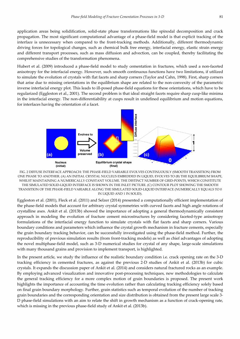
Phase‐field Modeling of Fracture Cementation Processes in 3‐D 81
application areas being solidification, solid‐state phase transformations like spinodal decomposition and crack
propagation. The most significant computational advantage of a phase‐field model is that explicit tracking of the
interface is unnecessary when compared to the front‐tracking methods. Additionally, different thermodynamic
driving forces for topological changes, such as chemical bulk free energy, interfacial energy, elastic strain energy
and different transport processes, such as mass diffusion and advection, can be coupled, thereby facilitating the
comprehensive studies of the transformation phenomena.
Hubert et al. (2009) introduced a phase‐field model to study cementation in fractures, which used a non‐faceted
anisotropy for the interfacial energy. However, such smooth continuous functions have two limitations, if utilized
to simulate the evolution of crystals with flat facets and sharp corners (Taylor and Cahn, 1998). First, sharp corners
that arise due to missing orientations in the equilibrium shape are related to the non‐convexity of the parametric
inverse interfacial energy plot. This leads to ill‐posed phase‐field equations for these orientations, which have to be
regularized (Eggleston et al., 2001). The second problem is that ideal straight facets require sharp cusp‐like minima
in the interfacial energy. The non‐differentiability at cusps result in undefined equilibrium and motion equations,
for interfaces having the orientation of a facet.
FIG. 2 DIFFUSE INTERFACE APPROACH: THE PHASE‐FIELD VARIABLE EVOLVES CONTINUOUSLY (SMOOTH TRANSITION) FROM
ONE PHASE TO ANOTHER. (A) AN INITIAL CRYSTAL NUCLEUS EMBEDDED IN LIQUID, EVOLVES TO (B) THE EQUILIBRIUM SHAPE,
WHILST MAINTAINING A NUMERICALLY CONSTANT VOLUME. THE DISTINCT NUMBER OF GRID‐POINTS, WHICH CONSTITUTE
THE SIMULATED SOLID‐LIQUID INTERFACE IS SHOWN IN THE INLET PICTURE. (C) CONTOUR PLOT SHOWING THE SMOOTH
TRANSITION OF THE PHASE‐FIELD VARIABLE ALONG THE SIMULATED SOLID‐LIQUID INTERFACE (NUMERICALLY EQUALS TO 0
IN LIQUID AND 1 IN SOLID).
Eggleston et al. (2001), Fleck et al. (2011) and Selzer (2014) presented a computationally efficient implementation of
the phase‐field models that account for arbitrary crystal symmetries with curved facets and high angle rotations of
crystalline axes. Ankit et al. (2013b) showed the importance of adopting a general thermodynamically consistent
approach in modeling the evolution of fracture cement microstructures by considering faceted‐type anisotropy
formulations of the interfacial energy function to simulate crystals with flat facets and sharp corners. Various
boundary conditions and parameters which influence the crystal growth mechanism in fracture cements, especially
the grain boundary tracking behavior, can be successfully investigated using the phase‐field method. Further, the
reproducibility of previous simulation results (from front‐tracking models) as well as chief advantages of adopting
the novel multiphase‐field model, such as 3‐D numerical studies for crystal of any shape, large‐scale simulations
with many thousand grains and provision to implement transport, is highlighted.
In the present article, we study the influence of the realistic boundary condition i.e. crack opening rate on the 3‐D
tracking efficiency in cemented fractures, as against the previous 2‐D studies of Ankit et al. (2013b) for cubic
crystals. It expands the discussion paper of Ankit et al. (2014) and considers natural fractured rocks as an example.
By employing advanced visualization and innovative post‐processing techniques, new methodologies to calculate
the general tracking efficiency for a more complex motion of grain boundaries is proposed. The present work
highlights the importance of accounting the time evolution rather than calculating tracking efficiency solely based
on final grain boundary morphology. Further, grain statistics such as temporal evolution of the number of tracking
grain boundaries and the corresponding orientation and size distribution is obtained from the present large scale 3‐
D phase‐field simulations with an aim to relate the shift in growth mechanism as a function of crack‐opening rate,
which is missing in the previous phase‐field study of Ankit et al. (2013b).

82 KUMAR ANKIT, MICHAEL SELZER, CHRISTOPH HILGERS, BRITTA NESTLER
Phase-Field Model
In the present section, we briefly recount the multiphase‐field model for the sake of completeness. The model
equations and numerical implementation have been previously discussed in detail (Stinner et al., 2004; Nestler et
al., 2005; Ankit et al., 2013b). The foundation of multiphase‐field method utilized to address crystal growth
problem is realized by a Helmholtz free energy functional formulated as
,Ω
(1)
where, is the bulk free energy density, ε is the small length scale parameter related to the interface width,
, is the gradient type and , a potential type energy density. Ω represents the volume of the numerical
domain, in consideration. The phase‐field parameter , , ··· , describes the location of `N’
crystals with different orientation in space and time. The interfaces between the different domains (represented by
phase‐field parameter) are identified by a continuous variation of the properties within a narrow region (Fig. 2), in
contrast to the front‐tracking approach for microstructure modeling. In equation 1, the integral extends over the
numerical domain in consideration and contains different free energy density contributions related either to the
interface or the bulk phase states. The gradient energy density , adds an energetic penalty on steep
interface transitions and is responsible for the broadening of the pre‐existing sharp interface. For the present
formulation, the antisymmetric gradient energy density is given by
, γ ,
,
, (2)
where is a normal vector to the αβ interface. γ is the magnitude of the surface energy
density. For the modeling of polycrystalline evolution in cemented fractures, it is desirable to use a faceted
solid/liquid surface energy anisotropy. In the present study, we use a piecewise defined function using the
maximum condition,
, max · , (3)
where k,αβ|k = 1,∙∙∙ ,ηαβ for ηαβ M denotes the complete set of vertex vectors of the corresponding equilibrium
shape of a crystal α embedded in the bulk phase β and M represents the number of edges. A detailed discussion on
selecting a relevant set of vertex vectors depending on the crystal equilibrium shape is presented in the following
sections. The evolution equations for the phase‐field vector components are described by variational derivative of
the free energy functional which ensures energy and mass conservation as well as an increase of total entropy.
· , , , , 1 , , . (4)
The symbol is the kinetic coefficient and comma separated sub‐indices represent derivatives with respect to
and gradient components
. The Lagrange multiplier guarantees the summation constraint ∑ 1
i.e.,
1 ∑ · , , , , , , .1 (5)
The phase‐field evolution equation (4) is non‐dimensionalised to ensure numerical accuracy during the
computation, as per the procedure explained by Wendler et al. (2009). Apparently, choosing an appropriate time
scale reduces the non‐dimesionalised form back to the original form (Equation 4) with the only exception of a
rescaling in the bulk free energy.
Modeling of Equilibrium Quartz
The complete set of `k’ vertices which are used to construct the anisotropic surface energy of quartz is presented in
Table 1. In order to simulate the precise equilibrium shape of a single quartz crystal growing in liquid, we adopt
the volume preservation approach, proposed earlier by Nestler et al. (2008). Derived interface energies of the facets
are given in Table 2. The polar‐plot of the interfacial energy and the corresponding equilibrium crystal shape are

Phase‐field Modeling of Fracture Cementation Processes in 3‐D 83
shown in Figs. 3a and 3b, respectively. The equilibrium shape represents an idealized quartz crystal consisting of
1010, 1011 and 0111 facets Lander et al. (2008); Lander and Laubach (2014). An implicit assumption of the
numerical simulations of the fracture cementation process, presented in the later sections of this article is that the
smaller crystal facets (21 1 1 and 6151 ) possess higher growth rate; hence, do not influence the final
polycrystalline morphology. Such fast‐growing and smaller facets are ignored in the present numerical studies.
However, it is to be noted that it is possible to simulate such facets, provided the polar‐plot of interfacial energy
(cusps) accounts for them. Hence, the assumption made in the present work should be interpreted as shape
simplification and not as a limitation of the simulation algorithm.
TABLE 1 THE `k’ VERTICES (REPRESENTED BY ηk,α/β IN EQUATION 3), WHICH IS USED TO GENERATE THE SURFACE ENERGY OF THE QUARTZ FACETS.
THE NUMBERS CORRESPOND TO THE RESPECTIVE VERTICES LABELED IN FIG. 3B.
Vertex Number x y z
1,2 0.000 0.000 ±1.000
3,4 ±0.152 ‐0.088 0.889
5 0.000 0.175 0.889
6 0.000 ‐0.175 ‐0.889
7,8 ±0.152 0.088 ‐0.889
9,10 ±0.152 0.437 0.556
11,12 ±0.455 ‐0.088 0.556
13,14 ±0.303 ‐0.350 0.556
15,16 ±0.152 ‐0.437 ‐0.556
17,18 ±0.455 0.088 ‐0.556
19,20 ±0.303 0.350 ‐0.556
21,22 ±0.505 0.000 0.444
23,24 0.253 ±0.437 0.444
25,26 ‐0.253 ±0.437 0.444
27,28 ±0.505 0.000 ‐0.444
29,30 0.253 ±0.437 ‐0.444
31,32 ‐0.253 ±0.437 ‐0.444
TABLE 2 DERIVED FACET ENERGIES FOR THE CHOSEN 3‐D QUARTZ GEOMETRY. THE INTERFACE FREE ENERGY PARAMETER, γαβ IS CHOSEN TO BE EQUAL TO
1.0 FOR BOTH SOLID/LIQUID AND SOLID/SOLID INTERFACES IN ALL THE SIMULATIONS.
Miller index Surface energy
(1 0 ‐1 0) 0.5γαβ
(1 0 ‐1 1) 0.9γαβ
(0 1 ‐1 1) γαβ
FIG. 3 (A) POLAR PLOT OF THE INTERFACIAL ENERGY FOR THE SYMMETRY OF A QUARTZ CRYSTAL. (B) EQUILIBRIUM QUARTZ
SHAPE OBTAINED FROM PHASE‐FIELD SIMULATION. THE COMPLETE SET OF VECTORS CORRESPONDING TO THE LABELED
VERTICES ARE PRESENTED IN TABLE 1. (C) THE DEFINITION OF CRYSTAL ORIENTATION IN 3‐D. THE RADIUS OF THE
HORIZONTAL CIRCLE GIVES A MEASURE OF THE MISORIENTATION WITH RESPECT TO THE MOST PREFERRED ORIENTATION OF
THE CRYSTALLOGRAPHIC C‐AXIS (WHICH IS ALONG Z AXIS FOR 3‐D QUARTZ). APPARENTLY, A CONCENTRIC CIRCLE WITH A
LARGER RADIUS REFERS TO A LARGER AXIAL TILT (OR LARGER MISORIENTATION) AND VICE VERSA. THE COLORS IN FIGURE 3B
AND 3C IS AN ILLUMINATION EFFECT TO DIFFERENTIATE AMONG CRYSTAL FACETS AND SHOULD NOT BE CONFUSED WITH
THE COLOR CODING USED TO REPRESENT CRYSTAL MISORIENTATION IN THE POLYCRYSTALLINE GROWTH.
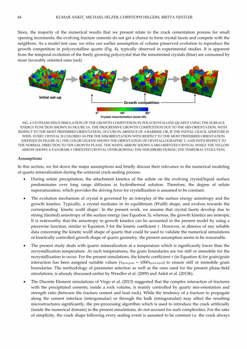
84 KUMAR ANKIT, MICHAEL SELZER, CHRISTOPH HILGERS, BRITTA NESTLER
Since, the majority of the numerical results that we present relate to the crack cementation process for small
opening increments, the evolving fracture cements do not get a chance to form crystal facets and compete with the
neighbors. As a model test case, we relax our earlier assumption of volume preserved evolution to reproduce the
growth competition in polycrystalline quartz (Fig. 4), typically observed in experimental studies. It is apparent
from the temporal evolution of the freely growing polycrystal that the misoriented crystals (blue) are consumed by
more favorably oriented ones (red).
FIG. 4 3‐D PHASE‐FIELD SIMULATION OF THE GROWTH COMPETITION IN POLYCRYSTALLINE QUARTZ USING THE SURFACE
ENERGY FUNCTION SHOWN IN FIGURE 3A. THE PROGRESSIVE GROWTH COMPETITION DUE TO THE MIS‐ORIENTATION, WITH
RESPECT TO THE MOST PREFERRED ORIENTATION, OCCURS IN ABSENCE OF A BARRIER, OR, IF THE INITIAL CRACK APERTURE IS
WIDE. EVERY CRYSTAL IS COLORED AS PER THE MISORIENTATION WITH RESPECT TO THE MOST PREFERRED ORIENTATION
(DEFINED IN FIGURE 3C) THE COLOR LEGEND SHOWS THE ORIENTATION OF CRYSTALLOGRAPHIC C‐AXIS WITH RESPECT TO
THE NORMAL DIRECTION TO THE GROWTH PLANE. THE WHITE ARROW SHOWS A MIS‐ORIENTED CRYSTAL WHILE THE YELLOW
ARROW SHOWS A FAVORABLY ORIENTED CRYSTAL OVERGROWING THE NEIGHBORS DURING THE TEMPORAL EVOLUTION.
Assumptions
In this section, we list down the major assumptions and briefly discuss their relevance in the numerical modeling
of quartz mineralization during the unitaxial crack‐sealing process.
During solute precipitation, the attachment kinetics of the solute on the evolving crystal/liquid surface
predominates over long range diffusion in hydrothermal solution. Therefore, the degree of solute
supersaturation, which provides the driving force for crystallization is assumed to be constant.
The evolution mechanism of crystal is governed by an interplay of the surface energy anisotropy and the
growth kinetics. Typically, a crystal nucleates in its equilibrium (Wulff) shape, and evolves towards the
corresponding `kinetic wulff shape’. In the present work, we assume that crystal facets develop due to
strong (faceted) anisotropy of the surface energy (see Equation 3), whereas, the growth kinetics are isotropic.
It is noteworthy that the anisotropy in growth kinetics can be accounted in the present model by using a
piecewise function, similar to Equation 3 for the kinetic coefficient τ. However, in absence of any reliable
data concerning the kinetic wulff shape of quartz that could be used to validate the numerical simulations
of kinetically controlled growth shape of quartz geometry, the present assumption seems to be reasonable.
The present study deals with quartz mineralization at a temperature which is significantly lower than the
recrystallization temperature. At such temperatures, the grain boundaries are too stiff or immobile for the
recrystallization to occur. For the present simulations, the kinetic coefficient τ (in Equation 4) for grain/grain
interaction has been assigned suitable values (τgrain,grain = 1000τgrain,liquid) to ensure stiff or immobile grain
boundaries. The methodology of parameter selection as well as the ones used for the present phase‐field
simulations, is already discussed earlier by Wendler et al. (2009) and Ankit et al. (2013b).
The Discrete Element simulations of Virgo et al. (2013) suggested that the complex interaction of fractures
with the precipitated cements, inside a rock volume, is mainly controlled by quartz mis‐orientation and
strength ratio (between the fracture cement and host rock). While the tendency of a fracture to propagate
along the cement interface (intergranular) or through the bulk (intragranular) may affect the resulting
microstructures significantly, the pre‐processing algorithm which is used to introduce the crack artificially
(inside the numerical domain) in the present simulations, do not account for such complexities. For the sake
of simplicity, the crack shape following every sealing event is assumed to be constant i.e. the crack always

Phase‐field Modeling of Fracture Cementation Processes in 3‐D 85
develop indiscriminately, along the cement/barrier sharp interface.
Numerical Aspects
With an objective to numerically simulate the crack‐seal process and to characterize the resulting microstructure,
we choose quartz crystals as a representative cement forming material. Fractal based models are considered to be
an efficient method for creating realistic‐appearing terrain Fournier et al. (1982). An algorithmically generated
(diamond‐square algorithm) fractal surface is utilized to model a 3‐D crack surface (boundary condition) for phase‐
field simulations (Fig. 5). The progressive fracturing of host‐rock and crystal precipitation in the open space is
algorithmically replicated once by numerical pre‐processing to obtain the initial condition for a simulation as
shown in Fig. 6. The preprocessing algorithm adopted is as follows:
The fractal topology of the lower crack surface is generated by a C program to implement the well‐known
diamond‐square algorithm (Miller, 1986). The topography (height‐map) of the upper crack surface is
obtained by subtracting the respective heights (for lower crack‐surface) from the total height of the parent
rock in consideration. The two complementary fractal surfaces are stationed over each other with a minor
clearance which represents the fracture in host rock.
The space between the upper and lower surface is increased (by 5 grid points in the fracture direction)
which represents the first crack‐opening event.
Crystals of equal size with different crystallographic orientation in space are initially laid on the lower crack
surface. At this point, it is important to note that the size of the crystal nuclei needs to be equal in order to
negate the advent of size‐effects in the following fracture cementation simulations. The numerical
preprocessing technique in order to rule out any such possibilities involves the following sub‐steps: Cuboid
crystal nuclei (different colors represent an axial tilt of the crystallographic axes defined in the previous
section) are generated separately and merged with the parent numerical domain containing the cleft (a
boundary condition) such that the former can be over‐written. The resulting domain can be described as a
perfectly sealed microstructure.
The lower crack surface is shifted downwards again to create a small space between the wall and crystal
front. Thus, we obtain the initial numerical domain to start the phase‐field simulations.
FIG. 5 (A) FRACTAL SURFACE (GENERATED BY A WELL‐KNOWN DIAMOND‐SQUARE ALGORITHM) USED FOR 3‐D CRACK‐SEALING
SIMULATIONS. (B) HEIGHT‐MAP OF THE GENERATED SURFACE.
At this point, we would like to clarify that the effectiveness of commonly used fractal techniques that are used to
model natural terrain, is a topic of ongoing debate. For the present studies, we choose the diamond‐square
algorithm due to simplicity and ease with which it can be computationally implemented. The primary intention of
using such a numerically‐constructed rough surface is to demonstrate the ability of the developed preprocessing
algorithm to design a relevant boundary condition (in 3‐D), for the simulation of fracture cementation process. In
past years, efficient algorithms have been developed to generate realistic surfaces (Lewis (1987); Arakawa and
Krotkov (1996)). However, a detailed comparison of such algorithms merit a separate discussion which in all
certainties, is neither the focus nor the highlight of the present work.
We simulate the unitaxial, one‐directional growth to investigate the formation of 3‐D crack‐sealing microstructure
using the initial condition generated in Fig. 6, and thereby, characterize the tracking behavior of grain boundaries

86 KUMAR ANKIT, MICHAEL SELZER, CHRISTOPH HILGERS, BRITTA NESTLER
and multi‐junctions. The following discussion will focus on the two 3‐D simulation test cases with the same initial
condition but different crack‐opening rate, as described in Table 3.
FIG. 6 SEQUENCE OF NUMERICAL PRE‐PROCESSING ADOPTED TO OBTAIN A HOMOGENEOUS OVERLAY (OF SAME SIZE) OF
CRYSTAL NUCLEI ON THE ALGORITHMICALLY GENERATED FRACTAL SURFACE. THE FINAL DOMAIN APPEARING IN THE
ABOVE SEQUENCE IS USED AS THE INITIAL CONDITION FOR PHASE‐FIELD SIMULATIONS TABLE 3 CHOICE OF NORMAL CRACK‐OPENING RATES FOR SIMULATIONS A AND B (∆x =∆y =∆z =1.0 AND ∆t =0.12). na AND nb REPRESENT THE CRACK‐
OPENING DISPLACEMENTS IN THE NORMAL DIRECTION FOR THE TEST CASES ‘a’ AND ‘b’, RESPECTIVELY (AS SHOWN IN FIG. 9).
Simulation Time between successive opening Opening increment
in vertical direction (N) Trajectory
A 2∆t 3∆x(NA) Quarter arc
B 2∆t 8∆x(NB) Quarter arc
The phase‐field evolution equation 4 is solved numerically using an explicit forward Euler scheme. The spatial
derivatives of the right hand side equation are discretized using a second order accurate scheme with a
combination of forward and backward finite differences. The implementation of a locally reduced order parameter
optimization employs a dynamic listing of a limited number of locally existing grains which enables us to reduce
computation time so that large scale simulations in 3‐D become feasible. The phase‐field simulations are performed
on Linux high‐performance computation clusters using a C program with parallel algorithms for domain
decomposition to distribute the computing task on different nodes.
FIG. 7 3‐D PHASE‐FIELD SIMULATION OF THE CRACK‐SEAL MICROSTRUCTURE. THE DIRECTION OF CRACK OPENING IS ALONG
THE QUARTER CIRCLE IN THE PLANE OF COMPUTATIONAL THIN‐SECTION (AS SHOWN BY THE BLUE ARROW IN THE OPENING‐
TRAJECTORY SCHEMATIC DIAGRAM). THE PRESENT SIMULATION SHOWS THE MORPHOLOGY OF GRAIN BOUNDARIES AFTER 400
CRACK OPENING AND SEALING EVENTS. (A) A 2‐D SECTION OF THE 3‐D COMPUTATIONAL MICROSTRUCTURE SUGGESTS
CONSUMPTION OF THE GRAIN MARKED BY WHITE ARROW. (B) A LOOK AT THE 3‐D COMPUTATIONAL MICROSTRUCTURE
REVEALS THAT THE GRAIN WAS ACTUALLY NOT CONSUMED; RATHER IT EVOLVED ALONG A DIFFERENT PLANE.
TRANSPARENCY OF THE SURROUNDING GRAINS ENABLE THE VISUALIZATION OF THE TRACKING CEMENT INSIDE THE
NUMERICAL DOMAIN.
As a result of wall rock opening along the predetermined opening trajectory, the crack‐aperture increases during
simulation run‐time. This adversely affects the computational efficiency as the size of simulation domain increases
in the fracture direction. In order to avoid such complications, the simulation is carried out in a moving frame (also
known as shifting‐box simulation). In the present simulations, the domain is shifted in the growth direction
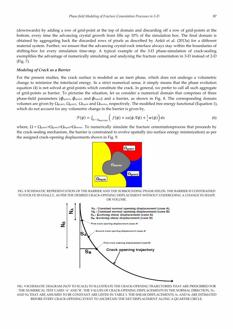
Phase‐field Modeling of Fracture Cementation Processes in 3‐D 87
(downwards) by adding a row of grid‐point at the top of domain and discarding off a row of grid‐points at the
bottom, every time the advancing crystal growth front fills up 10% of the simulation box. The final domain is
obtained by aggregating back the discarded rows of pixels as described by Ankit et al. (2013a) for a different
material system. Further, we ensure that the advancing crystal‐rock interface always stay within the boundaries of
shifting‐box for every simulation time‐step. A typical example of the 3‐D phase‐simulation of crack‐sealing
exemplifies the advantage of numerically simulating and analyzing the fracture cementation in 3‐D instead of 2‐D
(Fig. 7).
Modeling of Crack as a Barrier
For the present studies, the crack surface is modeled as an inert phase, which does not undergo a volumetric
change to minimize the interfacial energy. In a strict numerical sense, it simply means that the phase evolution
equation (4) is not solved at grid‐points which constitute the crack. In general, we prefer to call all such aggregate
of grid‐points as barrier. To picturise the situation, let us consider a numerical domain that comprises of three
phase‐field parameters ( grain1, grain2 and liquid) and a barrier, as shown in Fig. 8. The corresponding domain
volumes are given by Ωgrain1, Ωgrain2, Ωliquid and Ωbarrier, respectively. The modified free energy functional (Equation 1),
which do not account for any volumetric change in the barrier is given by,
,Ω Ω (6)
where, Ω = Ωgrain1+Ωgrain2+Ωliquid+Ωbarrier. To numerically simulate the fracture cementationprocess that proceeds by
the crack‐sealing mechanism, the barrier is constrained to evolve spatially (no surface energy minimization) as per
the assigned crack‐opening displacements shown in Fig. 9.
FIG. 8 SCHEMATIC REPRESENTATION OF THE BARRIER AND THE SURROUNDING PHASE‐FIELDS. THE BARRIER IS CONSTRAINED
TO EVOLVE SPATIALLY, AS PER THE DESIRED CRACK‐OPENING DISPLACEMENT WITHOUT UNDERGOING A CHANGE IN SHAPE
OR VOLUME.
FIG. 9 SCHEMATIC DIAGRAM (NOT TO SCALE) TO ILLUSTRATE THE CRACK‐OPENING TRAJECTORIES THAT ARE PRESCRIBED FOR
THE NUMERICAL TEST CASES ‘A’ AND ‘B’. THE VALUES OF CRACK‐OPENING DISPLACEMENTS IN THE NORMAL DIRECTION, NA
AND NB THAT ARE ASSUMED TO BE CONSTANT ARE LISTED IN TABLE 3. THE SHEAR DISPLACEMENTS, SA AND SB ARE ESTIMATED
BEFORE EVERY CRACK‐OPENING EVENT TO ASCERTAIN THE NET DISPLACEMENT ALONG A QUARTER CIRCLE.

88 KUMAR ANKIT, MICHAEL SELZER, CHRISTOPH HILGERS, BRITTA NESTLER
Quantifying Fracture Cement Tracking Characteristics
The term ’tracking efficiency’ (Urai et al., 1991) quantifies the tracking behavior of crack seal microstructures and is
governed by the roughness of the fracture wall, crack opening width and the ratio of crystal growth versus crack
opening rate (Hilgers et al., 2001; Nollet et al., 2005). Ankit et al. (2013b) amend this definition to a ’general tracking
efficiency’ (GTE) based on a fitting procedure for linear crack opening trajectory. It is to be noted that both the
above definitions of grain boundary tracking efficiency are based on the final microstructure morphology and do
not account for the temporal evolution of grain boundary tracking behavior. The dynamics of tracking efficiency is
particularly important when the wall roughness of the advancing crack surface is not sufficiently high and the
opening trajectory is non‐linear. For such cases, general tracking efficiency is numerically obtained by fitting a
straight lines in infinitesimally small time interval δt in which both the crack opening as well as grain boundary
morphology can be assumed to be linear. In the following section, we highlight the advantage of calculating
tracking efficiency by accounting for time evolution of grain barycenter (center of mass). We calculate the tracking
efficiency of the 3‐D computational microstructure by two different methods:
FIG. 10 LOCAL PEAKS OF CRACK SURFACE (REPRESENTED AS COLORED SPHERES) PLOTTED OVER THE ROCK‐CRYSTAL GROWTH
INTERFACE FOR SIMULATION A IN (A) AND (B) AND FOR SIMULATION B AS SHOWN IN (C) AND (D). THE FRACTAL PEAKS THAT
ARE TRACKED BY THE GRAIN BOUNDARIES/TRIPLE/QUADRUPLE JUNCTIONS ARE PLOTTED AS OFF‐WHITE SPHERES IN (A) AND
(C). THE FRACTAL PEAKS NOT TRACKED BY GRAIN BOUNDARIES/MULTI‐JUNCTIONS ARE PLOTTED AS LIGHT‐BLUE SPHERES IN
(B) AND (D). ON THE BASIS OF THE FINAL MICROSTRUCTURES, THE VALUES OF GTE (‘T’ BEING TOTAL TIME) FOR SIMULATION A
AND B ARE 0.685 AND 0.325 RESPECTIVELY. ON ACCOUNTING FOR TEMPORAL EVOLUTION, THE CORRESPONDING VALUES
DEPRECIATE TO 0.491 AND 0.206. THE GRAIN COLORS REFER TO THE AXIAL TILT INDEXED IN THE COLOR‐BAR.
1. The isosurfaces of the surviving crystals that are in contact with the advancing wall rock is visualized and the
local peaks of the facing crack surface are plotted. We employ a post‐processing algorithm which iteratively
inspects after every numerical time‐step, if a given grid‐point is a local peak among the k’ nearest neighbors
that lie along the barrier/grains sharp‐interface. For the present test cases A and B, we assume that ‘k’ equals 10.
The peaks of the fractal surface lying along the grain boundaries/multi‐junctions are extracted from the
computational microstructure of the simulations A and B (defined in Table 3) and are then superimposed, as
shown in Figs. 10a and 10c, respectively. The total number of the grain boundary/multi‐junction tracking peaks
is designated as Ntp. Similarly, those fractal peaks which neither lie along grain boundaries nor at multi‐

Phase‐field Modeling of Fracture Cementation Processes in 3‐D 89
junctions are plotted (Figs. 10b and 10d). The total number of such non‐tracking peaks is denoted by Nntp. The
general tracking efficiency (GTE) for the 3‐D crack‐seal microstructure is defined for the ith simulation time‐step
as:
GTE . 7
The definition of GTE is extended to account for the overall temporal evolution of tracking efficiency as:
GTE∑ · ∑ ·
(8)
where δt, n and t represent time‐step width, number of time‐steps and total simulation time respectively.
FIG. 11 (A) DIAGRAM EXPLAINING THE CALCULATION OF GTE2 WHICH ACCOUNTS FOR THE TEMPORAL EVOLUTION OF
TRACKING EFFICIENCY (GTE ). THE SOLID LINE REPRESENT THE EVOLUTION OF THE CRYSTAL BARYCENTER IN THE SHIFTING
BOX WHILE THE DASHED LINE CORRESPONDS TO CRACK‐OPENING TRAJECTORY. (B) IN ORDER TO ACCOUNT FOR THE
TEMPORAL EVOLUTION IN CALCULATION OF GENERAL TRACKING EFFICIENCY, THE BARYCENTER OF SURVIVING CRYSTALS
(IN CONTACT WITH ADVANCING CRACK SURFACE) IS DETERMINED. FOR THE SAKE OF BETTER VISUALIZATION, THE
BARYCENTER OF ONE OF THE SURVIVING CRYSTAL IS NUMERICALLY MASKED OVER ITS ISO‐SURFACE. THE GTE2 IS
CALCULATED BY INTEGRATING GTEI AS SHOWN IN EQUATION 10 FOR THE SURVIVING CRYSTALS WITH AXIAL TILTS OF (C) 5.63°
(D) 42.45° AND (E) 58.50° IN SIMULATION TEST CASE A AND (F) 5.63° (G) 7.16° AND (H) 32.01°, IN B.

90 KUMAR ANKIT, MICHAEL SELZER, CHRISTOPH HILGERS, BRITTA NESTLER
2. The second definition of grain boundary tracking efficiency takes into account the temporal evolution of the
barycenters of the surviving crystals in the shifting box, as described in the previous section. The actual
positions of the surviving crystal barycenters are obtained by adding the coordinates of the barycenters in the
shifting box with the total shift of the simulation box as shown for three tracking grains (Fig. 11).
For calculating the general tracking efficiency, the expression proposed by Ankit et al. (2013b) is redefined for a
small time interval δt and averaged over the total simulation time, according to
GTE∑ GTE ·
(9)
where, GTE . If δt is small, we rewrite the equation to
GTE
·
. (10)
The values of GTE1 and GTE2 are calculated for the two simulations A and B.
Simulation Results
Comparison of General Tracking Efficiencies
The resulting values for GTE1 and GTE2 are listed in Table 4 and it can be seen that the associated temporal
evolutions compare well. On the contrary, GTE and GTE derived from final microstructures, i.e. last simulation
time‐step differ significantly from GTE1 and GTE2 and show larger deviations with respect to each other.
Additionally, the estimated GTE2 vary with axial tilt and therefore, may lead to erroneous interpretation.
TABLE 4 CALCULATED GENERAL TRACKING EFFICIENCIES FOR THE SIMULATION TEST CASES, A AND B. CALCULATED VALUES gte2 ARE COMPARABLE TO
THE CORRESPONDING gte1 WHEREAS gte AND gte SHOW LARGER DEVIATIONS. THIS INDICATES THAT THE GENERAL TRACKING EFFICIENCIES COMPARE
QUITE WELL PROVIDED TEMPORAL EVOLUTION IS ACCOUNTED FOR ITS ESTIMATION.
Simulation A
Axial tilt GTE2 GTE1
5.63°
42.45°
58.5°
0.473
0.422
0.486
0.49
1 0.234
0.751
0.639 0.68
5
Simulation B
Axial tilt GTE2 GTE1
5.63°
7.16°
32.01°
0.166
0.204
0.196
0.20
6 0.167
0.254
0.131 0.32
5
Statistics
It is well known from the 2‐D numerical studies of crack‐seal process that a smaller crack‐opening rate favors the
formation of fibrous vein morphology, while, a larger crack opening rate leads to formation of blocky fracture
cements (Bons 2001; Hilgers et al., 2001; Ankit et al., 2013b). However, none of the previous studies focuses on the
statistical aspects which have the potential to provide valuable insights into the fracture cementation process.
We plot the number of grains surviving the crack opening process (in contact with the advancing crack surface)
versus the temporal crack opening distance and observe a shift between the two regimes, in the present 3‐D
simulations. As shown in Fig. 14a, the decline in the number of grains is significantly steeper if the crack opens at a
faster rate (simulation B), as compared to the case of slower opening (simulation A). The plummeting of grain
count is indicative of the anisotropy in surface energy being dominant, leading to orientation selection and growth
competition, similar to free‐growth conditions. In such a case, the misoriented grains are continuously eliminated
by favorably oriented neighbors. On the contrary, when the crack‐opening rate is smaller, the decrease in the
number of grains is less steep and becomes constant, which indicates that grain boundaries are pinned by fractal

Phase‐field Modeling of Fracture Cementation Processes in 3‐D 91
peaks on the fracture surface (Hilgers et al. (2001) call such peaks as Grain Boundary Attractors), even though the
general tracking efficiency is near about 0.5 (much lesser than 1.0). The grain size distribution in the shifting box
(final simulation time‐step) is plotted in Fig. 14b and represents those grains in contact with the advancing crack
surface for the test cases A and B. On comparison, it becomes clear that the tip of the distribution shifts towards
smaller mean grain sizes due to an increased pinning behavior of fractal peaks when the crack‐opening rate is
smaller. It is noteworthy that a major repercussion of grain‐boundary/multi‐junction pinning, as shown in Fig. 12,
is that the growth competition based on mis‐orientation is suppressed. In such cases, the consumption or survival
of a grain does not depend on mis‐orientation as shown in Fig. 13. Therefore, a higher number of grains survive the
crack‐sealing process as opposed to other case when crack‐opening rate is faster in evidence with the result in Fig.
14a.
FIG. 12 ANALYSIS OF THE TEMPORAL EVOLUTION OF A FRACTAL PEAK (IN SHIFTING BOX) WHICH PINS AT THE QUADRUPLE
POINT AND RESULTS IN GREATER TRACKING BEHAVIOR, AS EVIDENT FROM SURVIVAL OF MIS‐ORIENTED CRYSTAL FIBER (IN
BLUE). THE FRACTAL PEAK ILLUSTRATED AS A WHITE SPHERE ACTS AS A GRAIN BOUNDARY ATTRACTOR WHILE MOVING
ALONG A PREDETERMINED TRAJECTORY. IT IS INTERESTING TO NOTE THAT THE GRAIN QUADRUPLE JUNCTION ACTS AS A
STRONGER ATTRACTOR IN COMPARISON TO GRAIN BOUNDARIES, IN THE FINAL STAGES OF CRACK‐SEALING SIMULATIONS
(RIGHT IMAGE). THE AXIAL TILT OF THE GRAINS ARE INDEXED ACCORDING TO THE COLORBAR.
FIG. 13 TEMPORAL EVOLUTION OF MARKED AREAS IN SIMULATION A (SLOW CRACK‐OPENING) SHOW THAT THE PRECIPITATED
CEMENT FOLLOW THE TRAJECTORIES OF THE OPENING PEAKS AND EVOLVE INDEPENDENTLY OF THEIR MIS‐ORIENTATION,
WITH RESPECT TO THE MOST PREFERRED GROWTH DIRECTION. IN SUCH A CASE, THE GRAIN BOUNDARIES/MULTI‐JUNCTIONS
WHOSE MOTION IS PINNED BY THE PEAKS OF THE ADVANCING CRACK (SHOWN IN GRAY), TRACK THE OPENING TRAJECTORY.
THE COLOR OF THE GRAINS REPRESENT THE AXIAL TILT (NUMERICAL VALUES ALSO MENTIONED FOR GRAINS IN
CONSIDERATION) AND INDEXED AS PER THE COLORBAR.

92 KUMAR ANKIT, MICHAEL SELZER, CHRISTOPH HILGERS, BRITTA NESTLER
FIG. 14. STATISTICS OBTAINED FROM 3‐D PHASE‐FIELD SIMULATIONS. (A) NUMBER OF GRAINS IN CONTACT WITH THE
ADVANCING CRACK SURFACE PLOTTED AS FUNCTION OF NORMALIZED DISTANCE FROM THE POINT OF GREATEST
DEPRESSION ON THE NUCLEATION SURFACE. THE NUMBER OF GRAINS BECOME NEARLY CONSTANT WHEN GRAIN
BOUNDARIES/TRIPLE POINTS ARE PINNED AT FACING PEAKS FOR SMALL CRACK‐OPENING RATE. AT HIGHER CRACK‐OPENING
RATES, THE GROWTH COMPETITION DOMINATES DUE TO A LESSER ‘PINNING EFFECT’ EVIDENT FROM A DECREASING TREND,
EVEN AT LATER STAGES. (B) GRAIN SIZE DISTRIBUTION FOR THE FINAL MICROSTRUCTURES SHOWN IN FIG. 10. IN THE CASE OF
SLOWER CRACK‐OPENING, A SHIFT OF DISTRIBUTION PEAK TOWARDS SMALLER NORMALIZED GRAIN SIZE SIGNIFIES GREATER
PINNING LEADING TO HIGHER GRAIN BOUNDARY TRACKING EFFICIENCY.
Discussion of Results
The present work highlights the advantages of 3‐D numerical studies over 2‐D, by visualizing the complex and the
inherently 3‐D evolution of grain boundaries/multi‐junctions in crack‐sealing process.
Although, the idea of using the general tracking efficiencies (GTE), as defined by Ankit et al. (2013b) works well for
a 2‐D case, it is apparent that a similar procedure, in principle, cannot be employed for a general 3‐D case.
Moreover, the previous definition of GTE by Ankit et al. (2013b), do not account for the temporal evolution of
microstructures in the determination of tracking efficiency, which signifies the importance of present work. With a
motive to account for the temporal evolution of rock microstructures, we propose two different approaches to
determine the general tracking efficiencies and compare the results. We also clarify the main reason for the effect of
the crack opening rate on the grain growth statistics, i.e. on the number of grains tracking the opening trajectory,
size and orientation distribution.
For implementing a 3‐D fractal surface as the boundary condition and obtaining a uniform overlay of nuclei over
the crack surface which prevents the onset of size‐effects, preprocessing algorithms are proposed. An innovative
approach to visualize the numerically simulated fracture cements aided by post‐processing techniques reveals that
the grain boundary/multi‐junction morphologies in 3‐D are more complicated as compared to 2‐D cases, in general.
In order to deal with the third dimensionality which makes the determination of tracking efficiency difficult, we
amend the definition of general tracking efficiency to GTE1 and GTE2 given by equations (8) and (10) respectively.
While GTE1 may be interpreted as an extension of the tracking efficiency proposed by Urai et al. (1991) for the case
of 3‐D evolution, GTE2 accounts for the temporal change in tracking behavior of fracture cement with respect to the
crack‐opening trajectory. In contrast, GTE describes the tracking efficiency of the final microstructure (‘t’ being the
total simulation time) and does not account for temporal evolution. The study of peak trajectories demonstrate that
the GTE is significantly higher than GTE1 for the simulation test cases, A and B. It is noteworthy that GTE1 and
GTE2, both accounting for the temporal evolution of grain boundaries/multi‐junctions, compare quite well as
summarized in Table 4. The incongruousness arising out of the neglect of temporal evolution of grain
boundaries/multi‐junctions implies that conclusions about the tracking efficiency, as previously drawn upon the
GTE data, which solely rely on final microstructure have a clearly limited validity. While the original approach of
using grain boundary morphology to determine tracking efficiency proves to be inept in 3‐D, we conclude that the
proposed GTEs, both accounting the temporal evolution, serve as reliable methods to quantify the tracking
behavior in cemented fractures.
The grain evolution statistics obtained by post‐processing the 3‐D computational microstructure reveals that the

Phase‐field Modeling of Fracture Cementation Processes in 3‐D 93
number of grains in contact with advancing crack surface (Fig. 14a) decreases steeply when the crack‐opening rate
is higher. It can be argued that a steep decline in the number of grains and survival of crystals oriented along the
most preferred orientation, is indicative of growth competition, which does not relate to the boundary conditions
namely the crack surface roughness or the opening rate. The near incapability of fractal peaks to pin the grain
boundaries/multi‐junctions when crack‐opening rate is higher can be seen in Figs. 10c and 10d, where reddish
grains are found in majority. On the contrary, the decline in the number of grains is less steep for smaller crack
opening rate, which finally becomes constant. Such a statistic can be attributed to stronger pinning of fractal peaks
at grain boundaries and multi‐junctions, which suppresses the growth competition based on mis‐orientation of
neighboring grains (Fig. 13). An interesting outcome of visualizing the temporal evolution in Fig. 12, is that the
fractal peaks pin more strongly at quadruple junctions (grain multi‐junctions in general) as compared to grain
boundaries. The increase in pinning behavior of fractal peaks at smaller crack‐opening rates is further accentuated
by shift in the apex of grain size distribution towards small grain size (Fig. 14b). Thus, the plots of number of
surviving grains as well as grain size distribution (Fig. 14), provide a statistical realization of the shift in regime
and explain the fracture cement characteristics observed in Fig. 13, which is primarily governed by crack‐opening
velocity in the present test cases (different from curvature driven grain coarsening process).
Finally, it is worth clarifying that the present definitions of GTEs are formulated with an intention to indicate the
importance of temporal evolution in determining the tracking efficiency. We do not rule out the possibility of other
definitions, which may be equally capable of quantifying tracking behavior in 3‐D with high precision. Based on
the insights from the present numerical simulations, we assert that as long as the temporal evolution and the 3‐D
characteristics of the growing cement is accounted for, the derived tracking efficiency can, in principle, be
calculated correctly, irrespective of the technique used. Within the scope of current work, the prime motive is to
highlight the gain in accuracy by accounting for temporal evolution in the well known methodologies, which
strongly emphasizes the importance of 3‐D numerical studies. The growth statistics, obtained by accounting for
large number of grains and supplemented by 3‐D visualization, aims to bridge the gap between field observations
(of 3‐D layers) and computational studies (limited to 2‐D till date) and advances the understanding of the fracture
cementation process.
The current work which is based on a thermodynamically consistent approach, namely the phase‐field method
aims to fill‐in the short‐comings while focusing on the aspects that have not been addressed in the previous
numerical studies, chiefly the large‐scale statistical studies as well as complex motion of grain boundaries/multi‐
junctions in 3‐D. Wherever adequate, the benefits of 3‐D simulations have been highlighted while enumerating the
limitations of 2‐D studies. The 3‐D visualization aided by post‐processing techniques supplement the present
numerical studies and allow to draw meaningful conclusions from the simulation test cases. A close agreement of
both the general tracking efficiencies (GTE1 and GTE2) for the test cases ‘A’ and ‘B’, validates our findings and
confirms that the aim of conducting the numerical simulations has been adequately achieved. The most
outstanding achievement of the present work is the characterization of rock microstructures based on temporal
evolution of grain boundaries/multi‐junctions rather than relying on an approximate reconstruction from the final
morphology, a popular approach in the geoscientific community (Passchier and Trouw, 2005). Bearing in mind that
it is fundamentally (essentially) difficult to design as well as carry out in‐situ studies in laboratory experiments that
can replicate the process of fracture cementation (e.g., Hilgers et al. (2004); Okamoto and Sekine (2011)), the 3‐D
numerical studies are of paramount importance as they can alternatively provide invaluable insights into the
fracture cementation process. We further stress that the new methodologies based on multiphase‐field modeling
allow an efficient use of modern high super‐computing power, so that even the consideration of large grain
systems (up to 500,000 grains) in 3‐D computational studies becomes feasible.
Despite the reported advancement in the modeling framework, the quantitative comparison of the numerical
results with natural microstructures is not considered in the present work. In view of establishing a greater synergy
between the numerical modeling and field studies, the kinetics of mineral precipitation needs to be addressed.
Although, the kinetics of crack‐propagation in rocks may involve a different time‐scale as compared to fracture
cementation, it needs to be included in the present model for a more comprehensive study and direct comparison
with natural microstructures. The present modeling framework need to be developed in future, such that it can be
employed to derive macroscopic rheological laws that contain the microscopic reaction kinetics for given

94 KUMAR ANKIT, MICHAEL SELZER, CHRISTOPH HILGERS, BRITTA NESTLER
mechanical input configurations and can be used for enhanced transport modeling in the considered geological
systems.
Conclusions
The present phase‐field simulations of the fracture cementation process lead to following conclusions:
The microstructures simulated under respective boundary conditions show similarities with the natural
prototypes and generally agree with the previous numerical results of Urai et al. (1991), Hilgers et al. (2001)
and Nollet et al. (2006). The simulation may thus be upscaled to simulate reactive fluid flow and
corresponing in fractured reservoir rock.
The phase‐field method comes across as a valuable alternative to simulate the 3‐D fracture cementation
process.
The measurement of tracking efficiency in 3‐D for crack‐seal microstructures is relatively more cumbersome
as compared to 2‐D. In order to derive meaningful conclusions from the 3‐D numerical study, it is necessary
to analyze the out‐of‐plane evolution of grain boundaries, which turns out to be a non‐trivial task. Further,
it necessitates the employment of specialized techniques, for e.g. the ‘general tracking efficiencies’ proposed
in the current study which are essentially derived from the previous techniques of Urai et al. (1991) and
Ankit et al. (2013b).
Accounting for the temporal evolution of rock microstructure improves the accuracy of the estimation of
tracking characteristics that can be used to derive the deformation history. This leads to more advanced
models of evolving fracture cementation in reservoir rocks and its effect on fluid transport.
A more representative statistics obtained from 3‐D simulations (as compared to previous numerical studies
in 2‐D) contribute towards a better understanding of evolution mechanism whilst providing in‐situ
visualization of grain multi‐junctions and boundaries. The statistics and the visualization of the 3‐D fracture
cementation process show that grain quadruple junction acts as a stronger attractor in comparison to grain
boundaries, which has an additional effect on the final microstructure. However, for small crack increments
the crystallographic orientation of quartz grains does not affect the final microstructure.
Although the parameter varied in the study is limited to the crack‐opening rate, the 3‐D simulations
illustrate the advantages of adopting the phase‐field method and the employed visualization techniques in
studying fracture cementation. Therefore, the present work paves way for the 3‐D numerical studies to be
conducted for a wider bandwidth of parameters/boundary conditions.
ACKNOWLEDGMENT
K.A. and B.N. acknowledge the financial support by Graduate school 1483 of German Research Foundation and by
the project CCMSE of the European Union (EFRE) together with the state Baden‐Württemberg.
REFERENCES
[1] Ankit, K., Choudhury, A., Qin, C., Schulz, S., McDaniel, M., and Nestler, B. (2013a). Theoretical and numerical study of
lamellar eutectoid growth influenced by volume diffusion. Acta Materialia, 61(11):4245–4253.
[2] Ankit, K., Nestler, B., Selzer, M., and Reichardt, M. (2013b). Phase‐field study of grain boundary tracking behavior in
crack‐seal microstructures. Contributions to Mineralogy and Petrology, 166(6):1709 – 1723.
[3] Ankit, K., Selzer, M., and Nestler, B. (2014). Three‐dimensional phase field study of crack‐seal microstructures – insights
from innovative post‐processing techniques. Geoscientific Model Development Discussions, 7, 631‐658.
[4] Arakawa, K., and Krotkov, E. (1996). Fractal modeling of natural terrain: Analysis and surface reconstruction with range
data, Graphical models and image processing: GMIP 58(5), 413–436.
[5] Becker, S., Eichhubl, P., Laubach, S., Reed, R., Lander, R., and Bodnar, R. (2010). A 48 m.y. history of fracture opening,
temperature, and fluid pressure: Cretaceous Travis Peak Formation, East Texas basin, Geological Society of America Bulletin,

Phase‐field Modeling of Fracture Cementation Processes in 3‐D 95
122, 1081–1093.
[6] Becker, S., Hilgers, C., Kukla, P., and Urai, J. (2011). Crack‐seal microstructure evolution in bi‐mineralic quartz–chlorite
veins in shales and siltstones from the RWTH‐1 well, Aachen, Germany, Journal of Structural Geology, 33, 676 – 689.
[7] Bons, P. (2001). Development of crystal morphology during unitaxial growth in a progressively widening vein: I. the
numerical model. Journal of Structural Geology, 23(6–7):865 – 872.
[8] Bloch, S., Lander, R., and Bonnell, L. (2002). Anomalously high porosity and permeability in deeply buried sandstone
reservoirs: Origin and predictability, AAPG Bulletin, 86(2):301‐328.
[9] Bons, P., Koehn, D., and Jessell, M. (2008). Microdynamics Simulation, volume 106 of Lecture Notes in Earth Sciences. Springer
Berlin Heidelberg.
[10] Bons, P. D., Elburg, M. A., and Gomez‐Rivas, E. (2012). A review of the formation of tectonic veins and their
microstructures, Journal of Structural Geology, 43, 33 – 62.
[11] Durney, D. W. and Ramsay, J. (1973). Gravity and Tectonics, chap. Incremental Strains Measured by Syntectonic Crystal
Growths, pp. 67–96, New York: Wiley..
[12] Eggleston, J., McFadden, G., and Voorhees, P. (2001), A phase‐field model for highly anisotropic interfacial energy, Physica
D: Nonlinear Phenomena, 150, 91 – 103.
[13] Fleck, M., Mushongera, L., Pilipenko, D., Ankit, K., and Emmerich, H. (2011). On phase‐field modeling with a highly
anisotropic interfacial energy, European Physical Journal Plus, 126, 1–11.
[14] Fournier, A., Fussell, D., and Carpenter, L. (1982). Computer rendering of stochastic models, Communications of the ACM,
25, 371–384.
[15] Hilgers, C., Koehn, D., Bons, P., and Urai, J. (2001). Development of crystal morphology during unitaxial growth in a
progressively widening vein: II. Numerical simulations of the evolution of antitaxial fibrous veins, Journal of Structural
Geology, 23, 873 – 885.
[16] Hilgers, C., Dilg‐Gruschinski, K., and Urai, J. (2004). Microstructural evolution of syntaxial veins formed by advective flow,
Geology, 32, 261–264.
[17] Hubert, J., Emmerich, H., and Urai, J. (2009). Modelling the evolution of vein microstructure with phase‐field techniques –
a first look. Journal of Metamorphic Geology, 27(7):523–530.
[18] Jessell, M., Bons, P., Evans, L., Barr, T., and St¨uwe, K. (2001). Elle: The numerical simulation of metamorphic and
deformation microstructures. Computers and Geosciences, 27(1):17–30. cited By (since 1996)41.
[19] Koehn, D., Hilgers, C., Bons, P. D., and Passchier, C.W. (2000). Numerical simulation of fibre growth in antitaxial strain
fringes. Journal of Structural Geology, 22(9):1311 – 1324.
[20] Lander, R., Larese, R., and Bonnell, L. (2008). Toward more accurate quartz cement models: The importance of euhedral
versus noneuhedral growth rates. AAPG Bulletin, 92(11):1537–1563.
[21] Lander, R. and Walderhaug, O. (1999). Predicting porosity through simulating sandstone compaction and quartz
cementation. AAPG Bulletin, 83(2‐3):433–449.
[22] Laubach, S. E. (1997), A method to detect natural fracture strike in sandstone, AAPG Bulletin 81, p. 604–623.
[23] Laubach, S. E., R. M. Reed, J. E. Olson, R. H. Lander, and Bonnell, L. (2004a). Coevolution of crack‐seal texture and fracture
porosity in sedimentary rocks: Cathodoluminescence observations of regional fractures, Journal of Structural Geology 26,
967–982
[24] Laubach, S. E., J. E. Olson, and Gale J. F. W. (2004b). Are open fractures necessarily aligned with maximum horizontal
stress?, Earth and Planetary Science Letters, 222, 191–195.
[25] Lewis, J. P. (1987). Generalized stochastic subdivision, ACM Transactions on Graphics, 6(3), 167–190.
[26] Miller, G. S. (1986). Definition and rendering of terrain maps. Computer Graphics (ACM), 20(4):39–48.

96 KUMAR ANKIT, MICHAEL SELZER, CHRISTOPH HILGERS, BRITTA NESTLER
[27] Nestler, B., Garcke, H., and Stinner, B. (2005). Multicomponent alloy solidification: Phase‐field modeling and simulations.
Physical Reviews E, 71:041609.
[28] Nestler, B., Wendler, F., Selzer, M., Garcke, H., and Stinner, B. (2008). Phase‐field model for multiphase systems with
preserved volume fractions, Physical Reviews E, 78, 011604.
[29] Nollet, S., Urai, J., Bons, P., and Hilgers, C. (2005). Numerical simulations of polycrystal growth in veins, Journal of
Structural Geology, 27, 217 – 230.
[30] Nollet, S., Hilgers, C., and Urai, J. (2006). Experimental study of poly‐ crystal growth from an advecting supersaturated
fluid in a model fracture, Geofluids, 6, 185–200.
[31] Nüchter, J.A. & Stöckhert, B. (2007). Vein quartz microfabrics indicating progressive evolution of fractures into cavities
during postseismic creep in the middle crust. Journal of Structural Geology 29(9): 1445‐1462.
[32] Nüchter, J.A. & Stöckhert, B. (2008). Coupled stress and pore fluid pressure changes in the middle crust ‐ the vein record
of coseismic loading and postseismic stress relaxation, Tectonics 27, TC1007, doi:10.1029/2007TC002180.
[33] Passchier, C. and Trouw, R. (1996). Microtectonics. Springer‐Verlag Berlin Heidelberg, second edition.
[34] Ramsay, J.G. (1980). The crack–seal mechanism of rock deformation, Nature 284, 135 – 139.
[35] Selzer, M. (2014). Mechanische und Strömungsmechanische Topologieoptimierung mit der Phasenfeldmethode, Ph.D.
thesis, Department of Mechanical Engineering., Karlsruhe Institiute of Technology, Karlsruhe, Germany.
[36] Piazolo, S., Jessell, M., Bons, P., Evans, L., and Becker, J. (2010). Numerical simulations of microstructures using the elle
platform: A modern research and teaching tool. Journal of the Geological Society of India, 75(1):110–127.
[37] Stinner, B., Nestler, B., and Garcke, H. (2004). A diffuse interface model for alloys with multiple components and phases.
SIAM Journal on Applied Mathematics, 64(3):775–799.
[38] Taylor, J. E. and Cahn, J. W. (1998). Diffuse interfaces with sharp corners and facets: Phase field models with strongly
anisotropic surfaces. Physica D: Nonlinear Phenomena, 112(3–4):381 – 411.
[39] Urai, J., Williams, P., and van Roermund, H. (1991). Kinematics of crystal growth in syntectonic fibrous veins. Journal of
Structural Geology, 13(7):823 – 836.
[40] Virgo, S., Abe, S., and Urai, J. (2013). Extension fracture propagation in rocks with veins: Insight into the crack‐seal process
us ing discrete element method modeling, Journal of Geophysical Research: Solid Earth, 118(10), 5236 – 5251.
[41] Wendler, F., Becker, J., Nestler, B., Bons, P., and Walte, N. (2009). Phase‐field simulations of partial melts in geological
materials. Computers and Geosciences, 35(9):1907 – 1916.
[42] Zhang, J. and Adams, J. B. (2002). Facet: a novel model of simulation and visualization of polycrystalline thin film growth.
Modelling and Simulation in Materials Science and Engineering, 10(4):381.

Analysis, Interpretation, and Design of Inter‐
Well Tracer Tests in Naturally Fractured
Reservoirs Aymen A. Alramadhan*1, Ufuk Kilicaslan2, David S. Schechter3
Harold Vance Department of Petroleum Engineering, Texas A&M University, College Station, Texas, USA
[email protected]; [email protected]; [email protected]
Abstract
In order to understand the complex fracture network that controls water movement in a developed area within Spraberry Trend
in West Texas and to better manage the on‐going waterflood performance, a field scale inter‐well tracer test was implemented.
This test presents the largest inter‐well tracer test in naturally fractured reservoir reported in the industry and includes the
injection of 13 different tracers and sampling of 110 producers in an area covering 6533 acres.
This inter‐well tracer test generated a total of 598 tracer responses from 52 out of the 110 sampled producers. Tracer responses
showed a wide range of velocities from 14 ft/day to ultra‐high velocities exceeding 10,000 ft/day with same‐day tracer
breakthrough. Re‐injection of produced water has caused the tracers to be re‐injected and added an additional challenge to
diagnose and distinguish tracer responses affected by water recycling. This paper investigated analytical, numerical, and
inversion modeling approaches in order to categorize, history match, and connect tracer responses with water‐cut responses
with the objective to construct multiple fracture realizations based entirely on water‐cut and tracers’ profiles. In addition, the
research highlighted best practices in the design of inter‐well tracer tests in naturally fractured reservoirs through lessons
learned from this test.
Results indicated that tracer responses could be categorized based on statistical analysis of tracer recoveries with each category
showing distinguishing behavior in tracers’ movement and breakthrough time. In addition, it showed that tracer and water‐cut
responses in the lease are dominantly controlled by the fracture system revealing minimum information about the matrix
system. Numerical simulation studies showed limitations in dual porosity formulation/solvers to model tracer velocities
exceeding 2200 ft/day. Inversion modeling using Gradzone Analysis showed that east and north‐west of the developed area
have significantly lower pore volume compared to south‐west.
Keywords
Inter‐well Tracer Test; Tracer Resonse; Fractures Characterization; Naturally Fractured Reservoirs
Introduction
The successful implementation of tracer tests in the areas of petroleum reservoirs and groundwater fields over the
years has made those types of tests very reliable tool for reservoir description and characterization. Unlike pressure
transient tests which provide a low resolution description of the reservoir by averaging reservoir properties over
the bulk drainage volume, tracer tests have the ability to capture small scale features making it suitable for a more
detailed and a higher resolution reservoir description. In secondary and enhanced oil recovery projects, the degree
of success of economically recovering the remaining oil requires a robust understanding of fluid migration paths
and recovery mechanism in the reservoir.
The majority of inter‐well tracer tests have the main objective of assessing connectivity and direct communication
between injectors and producers. Other important objectives of inter‐well tracer tests include: identifying flow
anisotropy in the reservoir, evaluating sweep efficiency, identifying flow barriers, characterizing areal reservoir
heterogeneity, assessing reservoir layering, estimating fluid velocities, and determining offending injector(s) in
case of channeling. Once any or all of these objectives are met, the reservoir engineer will be able to design and
implement more efficient sweep improvement strategies ((1,2,3)).
Journal of Petroleum Science Research, Vol. 4 No. 2‐July 2015 97
2168‐5517/15/02 097‐26, © 2015 DEStech Publications, Inc.
doi: 10.12783/jpsr.2015.0402.05
*1 3

98 AYMEN A. ALRAMADHAN, UFUK KILICASLAN, DAVID S. SCHECHTER
When a pulse of injected tracer reaches the production well, the produced concentration will be a distributed tracer
response curve. This is due to water movement in the reservoir through a distribution of flow paths and different
flow rates within each path. A typical tracer response curve will show at least four distinctive landmarks as shown
in Figure 1: breakthrough time, maximum concentration produced, variance of response, and mean of the
distribution. Sweep efficiency is typically described in term of breakthrough time when it is plotted as a function of
cumulative water injection rate. In a one dimensional homogenous system, breakthrough is a measure of the swept
pore volume by injected water. In two or three dimensional heterogeneous system, breakthrough represents a
measure of the swept volume by only the highest conductive path between injector and producer. A nearly
instantaneous tracer breakthrough is an indication of fracturing. An early breakthrough with a sharp response is an
indication of water channeling through a high permeability and thin stringer. A late breakthrough is an indication
of poor communication or low transmissibility path between injector and producer ((1)).
The peak tracer concentration produced represents the mode of the tracer’s velocities distribution while the
variance of tracer distribution curve is dependent on local variation in flow velocity and/or on longitudinal
dispersion. The mean of tracer distribution represents the mean volume of water injected((1,7)).
Several researchers showed that multiple peaks in a tracer response can be extremely informative for reservoir
description. Abbaszadah showed that multiple peaks have strong correlation with the minimum number of
layers to match the tracer response. In addition, he indicated that if multiple peaks are observed to be close in
location to each other, it is an indication of substantial interference between layers contributing to tracer flow.
Datta‐Gupta et al. ((6)) showed that multiple peaks in a tracer response could be interpreted in term of correlated
and uncorrelated heterogeneity that reduce vertical and areal sweep efficiencies.
A thorough survey of the literature of large‐scale interwell tracer tests in naturally fractured reservoirs is presented
in Table 1 . The survey indicated that most of the tests were qualitative in nature and the general
conclusion was they were used only in a qualitative manner to assess injector‐producer connectivity without taking
advantage of other information carried within a full tracer response curve. The numerical simulation from
Spraberry Trend Area as reported by Schechter et al. indicated that extremely high fracture permeability (several
darcies) was required to history match tracer breakthrough and magnitude
simulation thus demonstrated the tremendous contrast between high fracture permeability and low average matrix
permeability (less than 1 md) in the area as determined by extensive core data. Case study highlighted in this
paper within Spraberry Trend Area in West Texas presents the largest inter‐well tracer test in naturally fractured
reservoir reported in the industry and includes the injection of 13 different tracers and sampling of 110 producers
in an area covering 6533 acres. This inter‐well tracer test generated a total of 598 tracer responses from 52 out of the
110 sampled producers. Case study presented in this paper is included in Table 1 for comparison purposes.
FIGURE 1: EXAMPLE OF A TYPICAL TRACER RESPONSE
((4,5))
. The ensuing dual porosity
((20,21,22,23))
((20))

Anlysis, Interpretation, and Design of Inter‐Well Tracer Tests in Naturally Fractured Reservoirs 99
TABLE 1: COMPARISON OF LARGE‐SCALE INTER‐WELL TRACER TESTS IN NATURALLY FRACTURED RESERVOIRS
Background of Spraberry Trend
The Spraberry Trend Area in West Texas was considered to be the largest oil field in the world at the time of its
discovery in 1949 with 8‐10 billion barrels of original oil in place ((8)). Spraberry is composed of naturally fractured,
low permeability siltstone which makes it problematic for both primary production and waterflooding ((9)). Based
on primary recovery, its original recovery factor was projected to be less than 10% . This low anticipated
recovery was the main drive to initiate waterflooding projects in several areas of Spraberry in late 1950s.
Unexpectedly, waterflooding projects in Spraberry showed very limited success where areas subjected to more
than 40 years of waterflooding showed less than 15% oil recovery ((9)). Reasons for the low waterflood recovery are
still not fully understood. Several hypotheses were developed to explain the wide‐scale poor performance
waterflooding ((12,13,14)). Those include: low matrix permeability and extensive fracturing ((15)), incorrect well pattern
alignment, fracture mineralization, lack of pattern confinement and injection well density , low effective
permeability to oil ((13)), and stress‐sensitive fracture conductivity ((14)).
Inter-well Tracer Test in the Developed Area within Spraberry Trend
Production History & Tracer Project Description
The developed area within Spraberry Trend was first put on production in mid of 1951. The oil production was dry
for about 22 years until the first water breakthrough occurred in early 1973. Early water production data shows
complex water‐cut behavior indicating the presence of a complex fracture system. Example of such water‐cut
behavior is shown in Figure 2. Water injection in this lease started in January 1983 after around 32 years of primary
depletion with one power water injector. Additional injector was introduced in 1990 and three more were
introduced in late 2001 / early 2002. Lease performance plots from July 1951 until March 2012 are shown in Figures
3 and 4.
In 2010, a decision was made to develop a large area of Spraberry using 11 inverted 9‐spot patterns. In order to
effectively manage the pattern water flood area as well as the area outside the pattern, 13 different non‐reactive
water tracers were injected through 13 injectors and 110 producers were water sampled. Objectives of this inter‐
well tracer test are to understand complex water movement in the reservoir, to assess injector‐producer
connectivity, and to understand sweep and fractures heterogeneity. The tracer test lasted for 114 days from start of
first tracer injection in April 25, 2011 until the analysis of the last water sample in August 17, 2011. Tracer
((10,11))
((16))
Author
Field , location
Tagged
injectors
Sampled
producers
Number of
Tracer Responses
Study Approach
Study
Year
Nitzberg, et.
al.
North West Fault
Block, Prudhoe Bay,
Alaska
22
53
> 46
Qualitative
1992
McConnell et.
al.
A Devonian Lower
Nisku dolomite
formation,
Albarta, Canada
5
20
20
Qualitative
2002
Schechter,
D.S. et. al.
Spraberry Trend,
O’Daniel Unit, West
Texas
6
29
45
Numerical Simulation
2002
Husain Zaberi
et. al.
A giant carbonate oil
field,
Saudi Arabia
5
65
7
Analytical
2008
Alramadhan
et. al
Spraberry Trend,
West Texas
13
110
598
Analytical, statistical
and numerical
2013

100 AYMEN A. ALRAMADHAN, UFUK KILICASLAN, DAVID S. SCHECHTER
breakthrough was observed from the same day of tracer injection, and a total of 598 tracer elution curves were
detected from 52 out of the 110 sampled wells. Tracer injection and sampling locations are shown in Figure 5. It
should be noted that rose diagram in Figure 5 was built using core and dynamic data from nearby leases and the
blue ellipses reflects areas where lease operator believe it is swept by injected water.
FIGURE 2: EXAMPLE OF EARLY COMPLEX WATER‐CUT BEHAVIOUR OBSERVED WITHIN AREA UNDERSTUDY
FIGURE 3: LEASE OIL AND WATER PRODUCTION RATES AND LEASE WATER‐CUT WITH TIME.
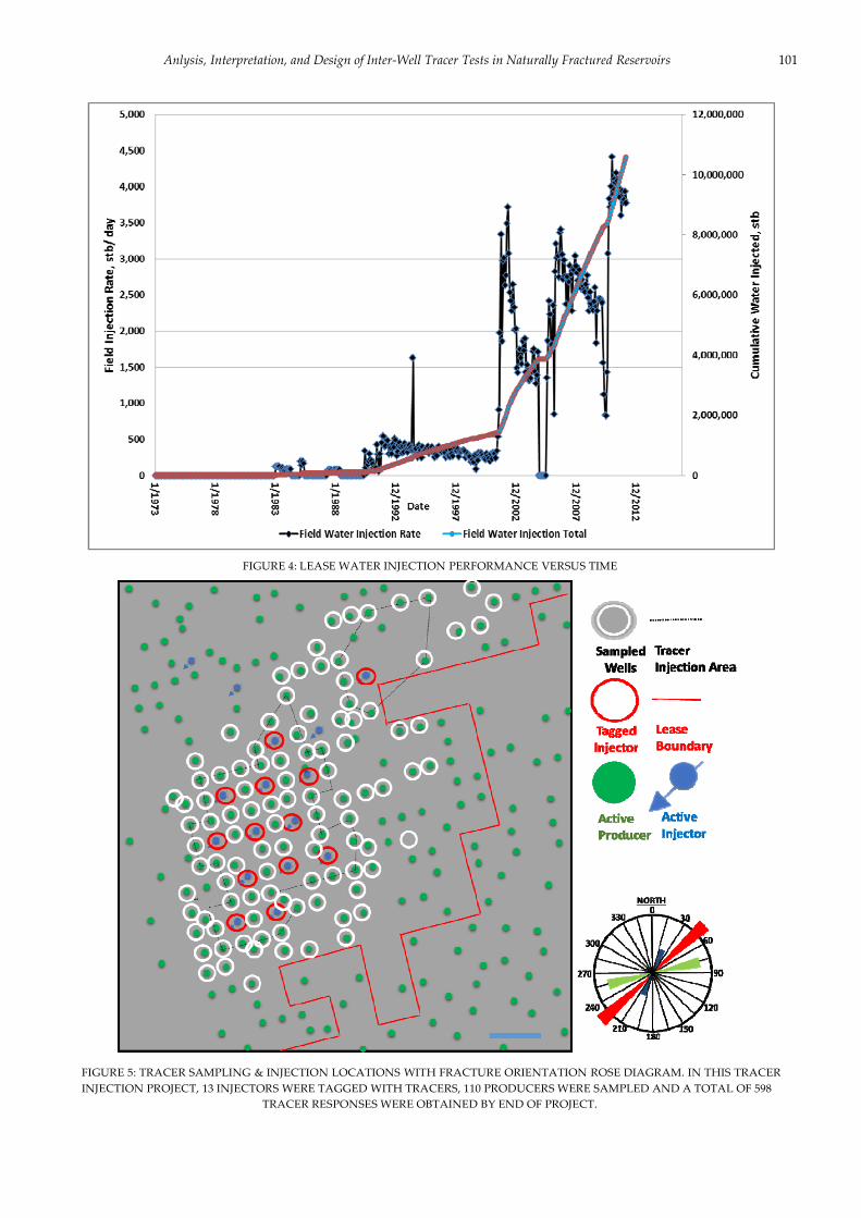
Anlysis, Interpretation, and Design of Inter‐Well Tracer Tests in Naturally Fractured Reservoirs 101
FIGURE 4: LEASE WATER INJECTION PERFORMANCE VERSUS TIME
FIGURE 5: TRACER SAMPLING & INJECTION LOCATIONS WITH FRACTURE ORIENTATION ROSE DIAGRAM. IN THIS TRACER
INJECTION PROJECT, 13 INJECTORS WERE TAGGED WITH TRACERS, 110 PRODUCERS WERE SAMPLED AND A TOTAL OF 598
TRACER RESPONSES WERE OBTAINED BY END OF PROJECT.

102 AYMEN A. ALRAMADHAN, UFUK KILICASLAN, DAVID S. SCHECHTER
Effect of Water Recycling
In the test area, the produced water from all wells flows through surface pipelines to a re‐injection facility. The re‐
injection of produced water has also caused the tracers to be re‐injected and to affect the results of the tracer test.
Measurement of tracers’ concentration at re‐injecting facility has been made and reported as part of the test.
Analytical Tracer Interpretation Techniques
Analytical tracer interpretation techniques are any type of interpretation that does not require building and
running numerical simulation models. This includes analyzing tracers responses using Method of Moments
(MOM), searching for data patterns in tracer or water‐cut responses, analyzing distributions of tracer recovered,
tracer velocities, and tracers’ breakthrough time, assessing layering from multiple peaks in tracers’ responses,
mapping observations, and making links between tracers responses and wells’ or lease performance.
Methods of Moment
Net swept volume calculations using moment analysis require three basic entries: produced tracer concentration,
water production and injection rates during tracer production . This is done for each injector‐producer pair
where tracer production is detected. In order to map directions of maximum swept volumes, all volumes were
normalized by dividing by the maximum value. Figure 6 shows distribution of lease‐wide net swept volumes
(normalized). The full field distribution of normalized net swept volume appears to be very close to a normal
distribution. This is most likely a reflection of the distribution of fracture properties within tracer‐flow area which
are the main drive of the sweep. Connecting wells that showed high swept volumes (normalized swept volumes ≥
0.50) consistently show four major flow features oriented N76oE. These major flow features highlighted in green in
Figure 7 were detected by 10 out of the 13 tagged injectors. For these 10 injectors to be widely spaced covering a
large area of the lease and consistently detecting these four flow features, it is an indication that these flow features
are inter‐connected and governs the majority of injected water movement in the tracer test area. Honoring high
swept volumes from Method of Moments and knowledge of fracture orientation from nearby areas, inter‐
connectivity could be explained by NE‐SW fractures connecting each of 10 injectors with these four major flow
features.
FIGURE 6: DISTRIBUTION OF NET SWEPT VOLUMES FROM METHODS OF MOMENTS WAS FOUND TO BE CLOSE TO A NORMAL
DISTRIBUTION. IT’S BELIEVED THAT THIS IS REFLECTIVE OF THE DISTRIBUTION OF FRACTURE PROPERTIES THAT CONTROLS
WATER MOVEMENT WITHIN AREA UNDERSTUDY
((7))

Anlysis, Interpretation, and Design of Inter‐Well Tracer Tests in Naturally Fractured Reservoirs 103
FIGURE 7: MAPPING MAXIMUM NORMALIZED NET SWEPT VOLUME FROM METHODS OF MOMENTS SHOWED
INTERCONNECTIVITY OF PATTERN PRODUCERS (GREEN) THROUGH NE‐SW FRACTURES (PINK). THESE INTER‐CONNECTED
PATHS WERE CONFIRMED BY 10 OUT OF 13 INJECTORS TAGGED WITH TRACERS. FRACTURE ORIENTATION ROSE DIAGRAM FROM
OTHER AREAS WITHIN SPRABERRY TREND IS SHOWN IN THE FIGURE.
Tracers Recoveries: Statistical Analysis & Categorizing Responses
Although the injection system was tagged with tracers, overall recovery was poor with none of the 13 injected
tracers showing more than 10% recovery. Such low tracers’ recoveries are not expected in a reservoir where highly
conductive fractures are believed to be the main drive for the high water‐cut observed in the lease. The main
reason for such poor tracers’ recoveries, as next sections will show, is that the developed area receives substantial
water influx from injection activities in neighboring leases causing it to be excessively diluted. A summary of total
tracer recovered for each of the 13 tracer is shown in Figure 8. Distribution of tracer recoveries for the 598 tracer
responses obtained in this study is shown in Figure 9. As shown in Figure 9, majority of tracer responses in this
inter‐well tracer test exhibit less than 0.01% tracer recovery (52.2% of tracer responses). These responses show
similarities in term of excessive dilution and non‐peaking trend which suggest that they could be studied as one
category. The next interval from 0.01‐0.1% shows a different frequency trend compared to tracers with < 0.01%
recovery. Similarities in the number of tracer responses observed within this interval suggest that these three
intervals could be combined into one category. In a similar manner, tracer responses with recoveries between 0.1‐
0.5% as well as tracer responses with recovery higher than 0.5% could be combined into two additional categories.
Although the last two categories still show low tracer recoveries, they are expected to be containing the maximum
useful information about tagged water movement in developed area.
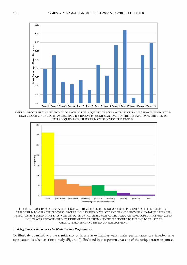
104 AYMEN A. ALRAMADHAN, UFUK KILICASLAN, DAVID S. SCHECHTER
FIGURE 8: RECOVERIES IN PERCENTAGE OF EACH OF THE 13 INJECTED TRACERS. ALTHOUGH TRACERS TRAVELLED IN ULTRA‐
HIGH VELOCITY, NONE OF THEM EXCEEDED 10% RECOVERY. SIGNIFICANT PART OF THIS RESEARCH WAS DIRECTED TO
EXPLAIN QUICK BREAKTHROUGH‐LOW RECOVERY PHENOMENA.
FIGURE 9: HISTOGRAM OF RECOVERIES FROM ALL TRACERS’ RESPONSES (COLOURS REPRESENT 4 DIFFERENT RESPONSE
CATEGORIES). LOW TRACER RECOVERY GROUPS HIGHLIGHTED IN YELLOW AND ORANGE SHOWED ANOMALIES IN TRACER
RESPONSES REFLECTED THAT THEY WERE AFFECTED BY WATER RECYCLING. THIS RESEARCH CONCLUDED THAT MEDIUM TO
HIGH TRACER RECOVERY GROUPS HIGHLIGHTED IN GREEN AND PURPLE SHOULD BE THE ONE TO BE USED IN
CHARACTERIZATION AND RESERVOIR MANAGEMENT.
Linking Tracers Recoveries to Wells’ Water Performance
To illustrate quantitatively the significance of tracers in explaining wells’ water performance, one inverted nine
spot pattern is taken as a case study (Figure 10). Enclosed in this pattern area one of the unique tracer responses
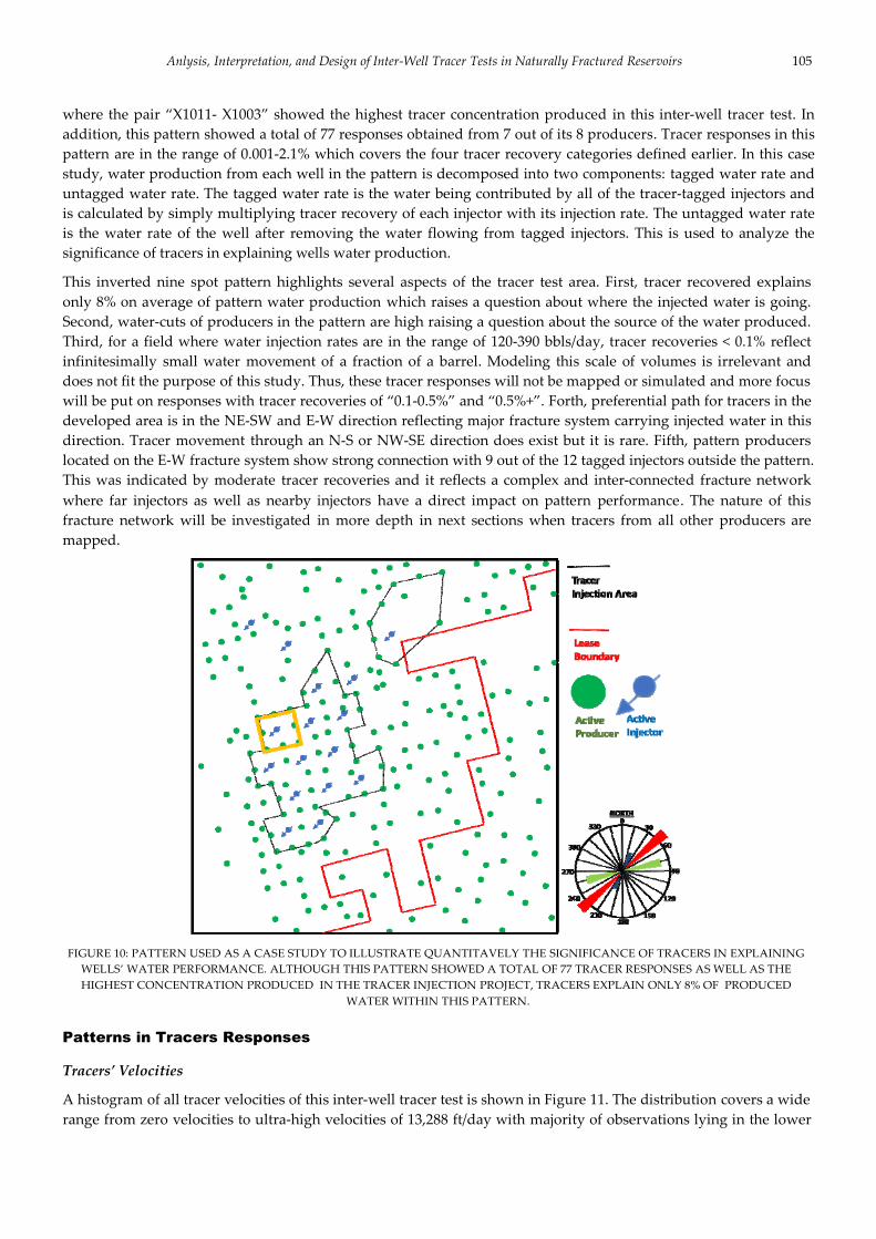
Anlysis, Interpretation, and Design of Inter‐Well Tracer Tests in Naturally Fractured Reservoirs 105
where the pair “X1011‐ X1003” showed the highest tracer concentration produced in this inter‐well tracer test. In
addition, this pattern showed a total of 77 responses obtained from 7 out of its 8 producers. Tracer responses in this
pattern are in the range of 0.001‐2.1% which covers the four tracer recovery categories defined earlier. In this case
study, water production from each well in the pattern is decomposed into two components: tagged water rate and
untagged water rate. The tagged water rate is the water being contributed by all of the tracer‐tagged injectors and
is calculated by simply multiplying tracer recovery of each injector with its injection rate. The untagged water rate
is the water rate of the well after removing the water flowing from tagged injectors. This is used to analyze the
significance of tracers in explaining wells water production.
This inverted nine spot pattern highlights several aspects of the tracer test area. First, tracer recovered explains
only 8% on average of pattern water production which raises a question about where the injected water is going.
Second, water‐cuts of producers in the pattern are high raising a question about the source of the water produced.
Third, for a field where water injection rates are in the range of 120‐390 bbls/day, tracer recoveries < 0.1% reflect
infinitesimally small water movement of a fraction of a barrel. Modeling this scale of volumes is irrelevant and
does not fit the purpose of this study. Thus, these tracer responses will not be mapped or simulated and more focus
will be put on responses with tracer recoveries of “0.1‐0.5%” and “0.5%+”. Forth, preferential path for tracers in the
developed area is in the NE‐SW and E‐W direction reflecting major fracture system carrying injected water in this
direction. Tracer movement through an N‐S or NW‐SE direction does exist but it is rare. Fifth, pattern producers
located on the E‐W fracture system show strong connection with 9 out of the 12 tagged injectors outside the pattern.
This was indicated by moderate tracer recoveries and it reflects a complex and inter‐connected fracture network
where far injectors as well as nearby injectors have a direct impact on pattern performance. The nature of this
fracture network will be investigated in more depth in next sections when tracers from all other producers are
mapped.
FIGURE 10: PATTERN USED AS A CASE STUDY TO ILLUSTRATE QUANTITAVELY THE SIGNIFICANCE OF TRACERS IN EXPLAINING
WELLS’ WATER PERFORMANCE. ALTHOUGH THIS PATTERN SHOWED A TOTAL OF 77 TRACER RESPONSES AS WELL AS THE
HIGHEST CONCENTRATION PRODUCED IN THE TRACER INJECTION PROJECT, TRACERS EXPLAIN ONLY 8% OF PRODUCED
WATER WITHIN THIS PATTERN.
Patterns in Tracers Responses
Tracers’ Velocities
A histogram of all tracer velocities of this inter‐well tracer test is shown in Figure 11. The distribution covers a wide
range from zero velocities to ultra‐high velocities of 13,288 ft/day with majority of observations lying in the lower

106 AYMEN A. ALRAMADHAN, UFUK KILICASLAN, DAVID S. SCHECHTER
velocities interval. For responses unaffected by water recycling, velocity distribution is very close to a tri‐modal
normal distribution (Figure 12). The three normal distributions most likely reflect three sets of fracture systems
each with different mean connectivity and fracture pore volume. This distribution can be an effective tool for
future fracture characterization studies as it provides an estimate of number of active fracture sets as well as
average properties for each. Basis for selecting tracer responses unaffected by water recycling is discussed in detail
in next section.
FIGURE 11: THREE TRENDS OBSERVED IN DISTRIBUTION OF TRACERS VELOCITIES. THE DISTRIBUTION COVERS A WIDE RANGE
FROM ZERO VELOCITIES TO ULTRA‐HIGH VELOCITIES OF 13,288 FT/DAY WITH MAJORITY OF OBSERVATIONS LYING IN THE
LOWER VELOCITIES INTERVAL.
FIGURE 12: TRI‐MODAL DISTRIBUTION OF TRACERS’ VELOCITIES OBSERVED WITHIN RESPONSES WITH 0.1‐0.5% RECOVERY. THE
THREE NORMAL DISTRIBUTIONS MOST LIKELY REFLECT THREE SETS OF FRACTURE SYSTEMS EACH WITH DIFFERENT MEAN
CONNECTIVITY AND FRACTURE PORE VOLUME. THESE DISTRIBUTIONS CAN BE AN EFFECTIVE TOOL FOR FUTURE FRACTURE
CHARACTERIZATION STUDIES AS IT PROVIDES AN ESTIMATE OF NUMBER OF ACTIVE FRACTURE SETS AS WELL AS AVERAGE
PROPERTIES FOR EACH.

Anlysis, Interpretation, and Design of Inter‐Well Tracer Tests in Naturally Fractured Reservoirs 107
Tracers’ Breakthrough Time
The global distribution of tracer breakthrough time is shown in Figure 13. It shows that majority of tracer responses
were obtained in the first two weeks of the project (64% of tracer responses). In addition, it shows a systematic
discontinuity starting from the third week of the test and continues in a cyclic manner. This study showed that this
cyclic behavior is only seen for tracer responses with both anomalies and very low recovery (<0.1%). It was
concluded that this behavior is associated with water recycling. As a result, only tracer responses obtained during
the first two weeks of the test were used for fracture characterization as those are less affected by water recycling.
FIGURE 13: DISTRIBUTION OF TRACERS’ BREAKTHROUGH TIME SHOWS THAT MAJORITY OF TRACER RESPONSES WERE
OBTAINED IN THE FIRST TWO WEEKS OF THE PROJECT (64% OF TRACER RESPONSES). IN ADDITION, IT SHOWS A SYSTEMATIC
DISCONTINUITY STARTING FROM THE THIRD WEEK OF THE TEST AND CONTINUES IN A CYCLIC MANNER. THIS RESEARCH
SHOWED THAT TRACERS RESPONSES OBTAINED WITHIN THIS INTERVAL WERE A RESULT OF WATER RECYCLING.
Single Peak & Multi‐Peak Responses
Multiple peaks in a tracer response reflect the degree of layering in the reservoir system. To evaluate how many
layers are needed to explain tagged water movement within the developed area of Spraberry Trend, the number of
peaks for all early tracer responses occurring during the first two weeks of the tracer test is evaluated and shown in
Table 2 below. In summary, majority of tracer responses show single peak tracer response (87.3% of total early
responses). Thus, movement of tagged water from a given injector to a given producer could be explained most of
the time by using a single layer model. Dual peaks and triple peaks tracer responses present only 11.4% and 1.3%
of total early responses, respectively. These less frequent responses could be explained by two and three layers
models. Table 3 shows that number of peaks in a tracer response shows a strong correlation with tracer recovery
indicating that as tracer recovery increases, the higher resolution the tracer response provides about the layering of
the system.
TABLE 2: FREQUENCY OF NUMBER OF PEAKS IN TRACERS’ RESPONSES.

108 AYMEN A. ALRAMADHAN, UFUK KILICASLAN, DAVID S. SCHECHTER
TABLE 3: PEAKING IN TRACERS RESPONSES LINKED TO TRACER RECOVERY CATEGORY
Mapping Tracers Recoveries
Mapping tracers recoveries highlighted two types of tracers movement in the reservoir: simple tracers movement
and complex tracers movement. The simple tracers movement is indicated by high tracers recoveries and is limited
to the vicinity of the injector’s wellbore in the E‐W and NE‐SW direction. On the other hand, the complex tracers
movement was indicated by moderate tracers recoveries and it highlighted the flow of injected water outside the
11 patterns injection area. In addition, it highlighted the complex inter‐connectivity between pattern injectors and
pattern producers. Simple tacers movement indicated by high tracer recoveries is shown in Figure 14 while
complex tracers movement indicted by moderate trecers recoveries is shown in Figure 15.
FIGURE 14: MAPPING FRACTURE NETWORK BY INTEGRATING ALL HIGH TRACER SHOWS. THIS FRACTURE NETWORK IS
CONFINED WITHIN PATTERN INJECTION AREA

Anlysis, Interpretation, and Design of Inter‐Well Tracer Tests in Naturally Fractured Reservoirs 109
FIGURE 15: MAPPING FRACTURE NETWORK BY INTEGRATING ALL MODERATE TRACER SHOWS. THIS FRACTURE NETWORK
HIGHLIGHTS THAT WATER FROM MAJORITY OF PATTERN INJECTORS IS ESCAPING PATTERN INJECTION AREA TOWARD THE
EAST.
Developed Area Production Performance
Overall analysis of production performance highlights several aspects of this development area. First, lease water
production closely follows the lease water injection indicating a poor waterflooding performance. Second, dry
production wells covering almost entire development area are shifted to very high water‐cuts in the range of 70‐
85% almost simultaneously in three months between July‐September 2002. Third, nature of injected water
breakthrough in this lease occurs simultaneously. This was observed from water breakthrough of 7 wells in 1973
and 44 wells in 2002. Fourth, no dry production is observed in development area after the global water
breakthrough in 2002. Recent inverted 9‐spot patterns introduced in 2010 show high initial water‐cut and poor
injection performance raising questions about the contribution of the water injected and the source of water
produced.
A Highlight on Dry Production History
The analysis of water production rate of the groups of wells that exhibited simultaneous water breakthrough in
1973 and 2002 shows three key findings: first, the simultaneous early water breakthroughs without any active
injection system in 1973 support the hypothesis of the presence of an external water source feeding the developed
area. Second, two out of four active injectors during 2002 are responsible for majority of the group water
production rate. This is evidenced by the match obtained between group water production rate and sum of wells
injection rates (Figure 16). Third, when developed area was subjected to water injection shutdown for 8 months
from late 2004 to mid of 2005, an abnormal increase in water‐cut of several producers was observed. This abnormal
increase in watercut was attributed to water influx to development area from an external water source.

110 AYMEN A. ALRAMADHAN, UFUK KILICASLAN, DAVID S. SCHECHTER
FIGURE 16: LEASE WATER PRODUCTION RATE FOLLOWS WATER INJECTION RATE IN THREE KEY PERIODS. FIGURE INDICATES
PERIODS WHERE WATER PRODUCED IS THE WATER INJECTED AS WELL AS PERIODS WHEN LEASE START RECEIVING WATER
FROM EXTERNAL INJECTION SOURCE.
Construction of Simulation Models
Multiple sectors and full‐field simulation models were built in order to run sensitivities and to model different
water‐cut and tracer responses observed in the developed area. Cases investigated are summarized in Table 4
below. In general, objectives of building simulation models include:
1. Assessing flow path characteristics by matching tracer breakthrough and peak concentration through high
resolution simulation models.
2. Assessing dilution and initial saturation uncertainty
3. Using pseudo wells to model loss of tracer & injected water outside study area.
4. Assessing average reservoir properties capable of explaining wells’ performance
TABLE 4: SUMMARY OF SIMULATION CASE STUDIES INVESTIGATED IN THIS STUDY
Case Study I: Matching Abnormal Tracers Velocities
Tracer flow between the well pair ‘S1012 – R‐18’ exhibited unique tracer response. Tracer traveled with a velocity
of 8,900 ft / day toward well ‘R‐18’ which exist outside patterns injection area. Tracer appeared 1 day after tracer
injection with the first water sampled. Although breakthrough was fast, the tracer response exhibited excessive
dilution showing tracer recovery of 0.3%. The tracer response and the locations of the two wells are shown Figure
17.
As sensitivities showed that tracer breakthrough time is primarily driven by fracture pore volume, Figure 18 below
shows the linear relation observed while attempting to match tracer breakthrough time by changing (ϕf h). The
slope of the line remains constant as long as the drawdown between the two wells remains unchanged. This linear
Case Objective
Case Study I Matching abnormal tracers velocities
Case Study II Modeling Tracer Flow outside Pattern Injection Area
Case Study III Modeling moderate and relatively high tracer responses within development area
Case Study IV Modeling Simultaneous field‐wide water breakthrough observed in year 2002
Case Study V Full Field Simulation Model to capture water and tracers movement

Anlysis, Interpretation, and Design of Inter‐Well Tracer Tests in Naturally Fractured Reservoirs 111
relation obtained through large number of simulation runs indicates that a breakthrough of 1 day is not
mathematically possible using fracture properties alone. This supports the hypothesis of the presence of an
external water source flowing to the developed area which creates both higher tracer velocities and excessive
dilution. This phenomenon is modeled by introducing a pseudo injector and a pseudo producer acting 1000 feet
away from development area to create a high drawdown across it. Figure 19 shows how the linear relation between
(ϕf h) product and tracer breakthrough time changes under different influx conditions. Due to numerical
limitations, the maximum achievable tracer velocity was 2,225 ft / day which represents only 25% of the actual
velocity observed.
FIGURE 17: RESPONSE OF TRACER TRAVELLED OUTSIDE PATTERN INJECTION AREA WITH ABNORMAL VELOCITY OF 8900 FT/DAY
( 1 DAY BREAKTHROUGH ). THIS RESPONSE IS STUDIED IN DEPTH IN SIMULATION CASE STUDY #1
FIGURE 18: LINEAR RELATION OBSERVED BETWEEN TRACER BREAKTHROUGH TIME AND (ϕF H) DURING MATCHING TRACER
RESPONSES.

112 AYMEN A. ALRAMADHAN, UFUK KILICASLAN, DAVID S. SCHECHTER
FIGURE 19 (SIMULATION CASE STUDY #1): TRACER BREAKTHROUGH TIME VERSUS (ϕF H) FOR DIFFERENT WATER INFLUX
CONDITIONS
Case Study II: Modeling Tracer Flow outside Pattern Injection Area
Matching moderate tracer velocities in the range of 669 – 853 ft /day was achievable by modifying (ϕf h) product as
mentioned in the previous case. Peak concentration was matched by modifying concentration injected to account
for dilution caused by water flow from nearby injectors. Figure 20 shows the example of a tracer response match
between the pair ‘S2114 ‐ R18’ using a fracture porosity‐thickness product of 0.006. Assuming a fracture porosity of
0.5%, these tracers reflect movement in highly stratified and fractured thin layers with 0.6‐1 ft extending for vast
distances outside tracer study area.
FIGURE 20 (SIMULATION CASE STUDY #2) : TRACER RESPONSE MATCH FOR WELL PAIR ‘S2114 ‐ R18’ WITH THEIR LOCATIONS.
TRACER MATCH PROVIDES A SOLUTION OF THE PRODUCT OF (ϕF H) BETWEEN THE PAIR OF INJECTOR AND PRODUCER.

Anlysis, Interpretation, and Design of Inter‐Well Tracer Tests in Naturally Fractured Reservoirs 113
Case Study III: Modeling Moderate and Relatively High Tracer Responses within Development Area
In a similar manner to case study II, tracer responses were matched by modifying (ϕf h) product of the layer and by
accounting for dilution from nearby wells. Both moderate and relatively high recovery tracer responses reflect
movement of tagged water in highly stratified and fractured thin layers. Moderate tracer recoveries reflect
movement of tagged water in a layer with (ϕf h) product in the range of 0.5 to 1.0x10‐3 ft. On the other hand, tracer
responses with relatively high recovery reflect movement of tagged water in a relatively thicker layer with (ϕf h)
product in the range of 0.85 to 3.0x10‐3 ft. Example of tracer match is shown in Figure 21 .
FIGURE 21 (SIMULATION CASE STUDY #3): TRACER RESPONSE MATCH FOR WELL PAIR ‘S1202 – S1809’ WITH MAP SHOWING THEIR
LOCATIONS. TRACER MATCH PROVIDES A SOLUTION OF THE PRODUCT OF (ϕF H) BETWEEN THE PAIR OF INJECTOR AND
PRODUCER.
Case Study IV: Modeling Simultaneous Field‐wide Water Breakthrough
A simulation model was built with the objective to match the simultaneous field‐wide water breakthrough and the
water production performance of 44 producers from 2002‐2009. Two approaches to model the problem were
followed: first approach is to model wells performance using initially dry simulation model (initial saturation =
Swir). Second approach is to model wells performance using initially wet simulation model (initial saturation >
Swir).
The first approach has the advantage of capturing the early dry production of all wells. It showed some success in
matching the water breakthrough time but did not show an acceptable water‐cut match. Figure 22 below shows the
best obtainable match for total water production rate using the first approach. It indicates that to achieve such
quick water breakthrough, the pore volume of the system has to be very small in the range of (ϕh) product of 0.75
or below.
The second approach has more flexibility to model water performance after breakthrough. It showed a remarkable
success in matching the water production performance but leaves the early dry oil production period unexplained.
Figure 23 shows multiple matches of development area water production and water‐cut, respectively. The multiple
matches indicate two important findings: first, water performance is dominantly driven by average water
saturation in the matrix‐fracture system. Second, the reservoir has a moderate matrix pore volume system of (ϕh)
product of 1.65. Different combinations of matrix porosity and thickness with the same product yield identical
solution.

114 AYMEN A. ALRAMADHAN, UFUK KILICASLAN, DAVID S. SCHECHTER
FIGURE 22 (SIMULATION CASE STUDY #4): BEST MATCH OF LEASE WATER PRODUCTION RATE OF 2002 WELLS USING DRY MODEL
APPROACH.
FIGURE 23 (SIMULATION CASE STUDY #4): MULTIPLE HISTORY MATCHES OF LEASE WATER PRODUCTION RATE OF 2002 WELLS
USING WET MODEL APPROACH. ALL REALIZATIONS HAVE SAME (ϕF H) OF
Case Study V: Full Field Simulation Model
A full field simulation model was built in order to model simultaneously the 13 tracers injected as well as
performances of all producers and injectors in development area. The selection of full field boundary was done
with precaution as tracer results showed interaction and ultra‐high velocity gradients between tracer study area
and surrounding. A selection of full field area should enclose all nearby water injection activity to capture history

Anlysis, Interpretation, and Design of Inter‐Well Tracer Tests in Naturally Fractured Reservoirs 115
of early water movement in the lease. The boundary for the full field model chosen for this study is shown in
Figure 24 below and it includes 23 injectors and 195 producers. The overall objectives of full field simulation model
include:
1. Assess average reservoir properties capable of explaining wells’ performance.
2. Investigate the modeling of 13 different tracers simultaneously using a full field simulation model.
3. Investigate well interference through fracture system and its effect on tracer solution.
Attempts to study tracer responses using full field simulation model have not been successful. The main reason
behind such unsuccess is the extreme sensitivity of tracer solution to size of gridcells and to any convergence
problem encountered by simulator. Due to this extreme sensitivity of tracer solution, a decision was made to use
the full field model only to match water‐cut responses.
Sensitivity runs showed that water‐cut response is driven dominantly by three parameters: initial water saturation
of matrix‐fracture system, thickness, and matrix porosity. While initial saturation could be inferred from initial
water‐cut of the well, average matrix porosity and thickness of the lease is estimated by trial and error. A matrix
porosity‐thickness product of 1.65 was found to match performance of several wells covering large area of the lease.
FIGURE 24: BOUNDARY OF FULL FIELD SIMULATION MODEL SELECTED FOR THE STUDY
Inversion Modeling Approaches
The process of history matching where parameters controlling reservoir performance is modified until an
acceptable match is achieved between simulated response and observed performance data is a process that has
been performed traditionally by trial and error. With the advancement of computational capabilities and
optimization approaches, new tools were developed to assist the reservoir engineer in such a process ((17)). These
tools define an objective function based on the difference between observed data and simulated responses, and use
gradient‐based optimization techniques to minimize the objective function . In this study, the objectives of
inversion modeling can be summarized as follows:
1. Invert water‐cut responses to predict fracture properties governing flow in reservoir.
((19))
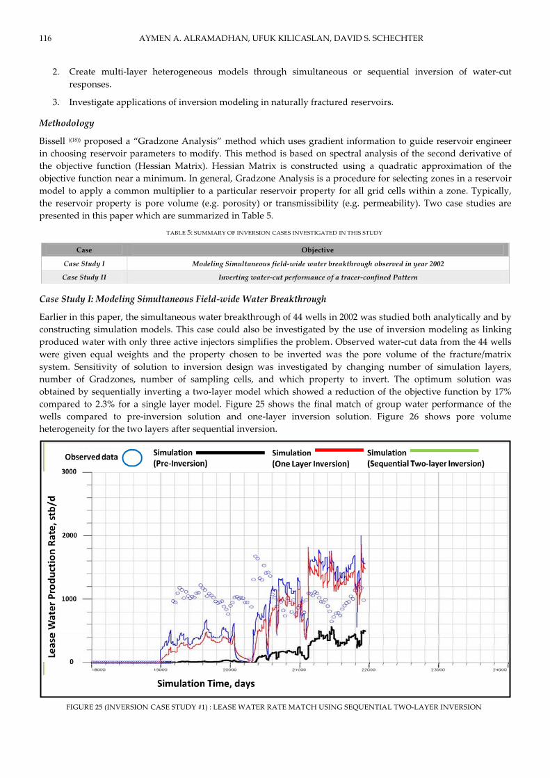
116 AYMEN A. ALRAMADHAN, UFUK KILICASLAN, DAVID S. SCHECHTER
2. Create multi‐layer heterogeneous models through simultaneous or sequential inversion of water‐cut
responses.
3. Investigate applications of inversion modeling in naturally fractured reservoirs.
Methodology
Bissell ((18)) proposed a “Gradzone Analysis” method which uses gradient information to guide reservoir engineer
in choosing reservoir parameters to modify. This method is based on spectral analysis of the second derivative of
the objective function (Hessian Matrix). Hessian Matrix is constructed using a quadratic approximation of the
objective function near a minimum. In general, Gradzone Analysis is a procedure for selecting zones in a reservoir
model to apply a common multiplier to a particular reservoir property for all grid cells within a zone. Typically,
the reservoir property is pore volume (e.g. porosity) or transmissibility (e.g. permeability). Two case studies are
presented in this paper which are summarized in Table 5.
TABLE 5: SUMMARY OF INVERSION CASES INVESTIGATED IN THIS STUDY
Case Study I: Modeling Simultaneous Field‐wide Water Breakthrough
Earlier in this paper, the simultaneous water breakthrough of 44 wells in 2002 was studied both analytically and by
constructing simulation models. This case could also be investigated by the use of inversion modeling as linking
produced water with only three active injectors simplifies the problem. Observed water‐cut data from the 44 wells
were given equal weights and the property chosen to be inverted was the pore volume of the fracture/matrix
system. Sensitivity of solution to inversion design was investigated by changing number of simulation layers,
number of Gradzones, number of sampling cells, and which property to invert. The optimum solution was
obtained by sequentially inverting a two‐layer model which showed a reduction of the objective function by 17%
compared to 2.3% for a single layer model. Figure 25 shows the final match of group water performance of the
wells compared to pre‐inversion solution and one‐layer inversion solution. Figure 26 shows pore volume
heterogeneity for the two layers after sequential inversion.
FIGURE 25 (INVERSION CASE STUDY #1) : LEASE WATER RATE MATCH USING SEQUENTIAL TWO‐LAYER INVERSION
Case Objective
Case Study I Modeling Simultaneous field‐wide water breakthrough observed in year 2002
Case Study II Inverting water‐cut performance of a tracer‐confined Pattern

Anlysis, Interpretation, and Design of Inter‐Well Tracer Tests in Naturally Fractured Reservoirs 117
FIGURE 26 (INVERSION CASE STUDY #1): MODEL HETEROGENEITY AFTER SEQUENTIAL TWO LAYER INVERSION: LAYERS 1 (TOP)
AND LAYER 2 (BOTTOM). INVERSION MODELING RESULTS SHOW THAT NORTH‐EAST AND WEST SIDES OF THE LEASE HAVE
VERY LOW PORE VOLUME COMPARED TO THE SOUTH‐EAST. NORTH‐EAST AND WEST SIDES OF LEASE HAVE 2% AND 35% OF
THE PORE VOLUME EXISTING IN THE NORTH‐EAST, RESPECTIVELY.
Case Study II: Inverting Water‐cut Performance of a Pattern
A high resolution sector model was built for one inverted 9 spot pattern that showed confined and moderate
concentration tracer responses. For the objective function, observed water‐cut data from three key wells were given
equal weights and the property chosen to be inverted was the pore volume of the system. Figure 27 below shows
the locations of the three key wells used in the objective function. Investigating different inversion designs under
variable initial water saturation, the optimum solution was obtained by inverting a one‐layer model which showed
a reduction of the objective function by 13.3%. Figures 28 and 29 show the model heterogeneity and wells’
performance before and after inversion.

118 AYMEN A. ALRAMADHAN, UFUK KILICASLAN, DAVID S. SCHECHTER
FIGURE 27 (INVERSION CASE STUDY #2): PATTERN USED FOR WATERCUT INVERSION
FIGURE 28 (INVERSION CASE STUDY #2): MATRIX / FRACTURE PORE VOLUME AFTER WATERCUT INVERSION OF A TRACER‐
CONFINED PATTERN. INVERSION RESULTS SHOW THAT MAJORITY OF PORE VOLUMES WITHIN PATTERN ARE CONCENTRATED
AROUND THREE KEY PRODUCERS. THIS EXPLAINS THE CONFINEMENT OF THE TRACER USED IN THIS CASE STUDY.

Anlysis, Interpretation, and Design of Inter‐Well Tracer Tests in Naturally Fractured Reservoirs 119
FIGURE 29 (INVERSION CASE STUDY #2): WATERCUT MATCH OF EXAMPLE WELL (PRE AND POST WATERCUT INVERSION).
Design Aspects of Inter-well Tracer Test
Lessons learned from this inter‐well tracer test could be summarized as follows:
1. Volume of injected tracers used was excessively large. Only 18% of the volumes used were required to
capture and characterize the complex fracture network in the field. Using a combination of low detection
limit and excessive tracer volume was the main reason of creating high number of excessively diluted
responses that added no value to characterization process.
2. Sampling of water produced should start from same day of tracer injection in order to avoid missing
breakthrough time of ultra‐high velocity tracers.
3. Sampling of water produced for tracer concentration measurements should have been terminated by the
second week when majority of tracers responses turned to be intermittent and excessively diluted. This
could have saved 87.7% of operating time without effecting test interpretation.
Conclusions
The research presented in this paper could be workflowed into three key phases: analytical interpretation,
numerical modeling, and inversion modeling phase. Analytical interpretation phase was successfully used to
achieve several key objectives: first, to build a robust pre‐simulation understanding of preferential water
movement directions within pattern area under study. Second, it was used as a data mining exercise to classify
which group of tracer responses carries the most useful information in characterizing and managing the lease.
Third, it helped to identify tracer responses highly affected by water recycling. Fourth, it identified a common
direction where injected water is leaving the inverted 9‐spot pattern development area to outside the lease.
For numerical simulation phase: first, it was used to investigate tracer flow formulation in dual porosity media to
identify what reservoir characterization information is carried within a tracer response. Second, it was used to test
limitations of dual porosity formulation to model ultra high velocities tracers. Third, it was used to test modeling
13 different tracers simultaneously in a full‐field case.
For inversion modeling phase, an attempt was made to test capabilities of dual porosity inversion packages on a
pattern level where tracers showed confined injection as well as on a field level to capture the nature of
simultaneous water breakthrough observed in the field.
Conclusions based on the research findings could be summarized as follows:
1. Maximum sweep directions obtained from Methods of Moments indicate the presence of four major inter‐
connected flow features oriented N76oE governing water movement in the field.

120 AYMEN A. ALRAMADHAN, UFUK KILICASLAN, DAVID S. SCHECHTER
2. Poor overall tracer recovery with none of the 13 injected tracer recovered by more than 9%.
3. Tracers recovered explain no more than 10% by average of patterns’ water production
4. Tracers responses could be categorized into four groups based on the distribution of tracer recovery for all
tracers’ responses.
5. Studying patterns of tracer responses based on tracer recovery highlights several aspects:
a. Tracer responses with less than 0.01% recovery are highly affected by water recycling. As tracer
recovery of the tracer response increases, the water recycling effect decreases.
b. Velocity distribution of responses unaffected by water‐recycling shows a tri‐modal normal distribution.
These distributions could serve as a powerful tool for future fracture characterization studies to
estimate average properties of each set of fracture.
c. Number of peaks in a tracer response correlates strongly with tracer recovery. This indicates that a
higher recovery tracer response captures more the layering between a pair of injector and producer.
6. The development area within Spraberry Trend receives water influx from an external water source. This is
supported by the following observations:
a. The extensive instantaneous dilution and the abnormal tracer velocity of 8,900 ft/day for a tracer
travelled across the lease outside pattern injection area.
b. The absence of a mathematical solution using dual porosity formulation to describe a tracer velocity of
8900 ft/day based on fracture properties alone.
7. Breakthrough time of tracer responses provides a solution for (ϕf h) of the fracture layer. Peaks of tracer
responses are highly affected by dilution and are not a reliable measure of any fracture property.
8. All investigations carried through numerical simulation modeling highlighted that the lease of dynamic
response is dominantly governed by fractures revealing minimum information about the matrix system.
Such very weak fracture‐matrix communication is most likely caused by high degree of fracture
mineralization.
9. Majority of pattern injectors, 6 out of 11, show that part of the injected water flow outside the development
area toward east. Although tracers indicate small volumes, these volumes could be underestimated by
excessive tracer dilution
10. Inversion modeling results show that north‐east and west side of the lease have very low pore volume
compared to the south‐east. North‐east and west side of lease have 2% and 35% of the pore volume existing
in the north‐east, respectively.
ACKNOWLEDGMENT
The authors would like to express their gratitude to Dr. David S. Schechter for his continuous support and
encouragement to publish this work and for Harold Vance Department of Petroleum Engineering at Texas A&M
University for all resources that made this work where it is today.
REFERENCES
[1] Allison, Steven Bradley (1988). Analysis and design of field tracers for reservoir description. Master’s thesis, The
University of Texas at Austin.
[2] Oyerinde, Adedayo Stephen (2004). A composite tracer analysis approach to reservoir characterization. Masterʹs thesis,
Texas A&M University.
[3] Alkouh, A.B. and Chen, H.‐Y. 2008. Flow Anisotropy Analysis from Multiwell‐Testing of Sabiriyah Field, North Kuwait.
[4] Abbaszadeh‐Dehghani, M. and Brigham, W.E., “Analysis of Unit Mobility Ratio Well‐to‐Well Tracer Flow to Determine
Reservoir Heterogeneity,” U.S. DOE Report SF/11564‐1, Feb. 1983.

Anlysis, Interpretation, and Design of Inter‐Well Tracer Tests in Naturally Fractured Reservoirs 121
[5] Abbaszadeh‐Dehghani, M. and Brigham, W.E. 1984. Analysis of Well‐to‐Well Tracer Flow to Determine Reservoir
Layering. Journal of Petroleum Technology 36 (10): 1753‐1762. DOI: 10.2118/10760‐pa
[6] Streamline Simulation : Theory and Practice. Akhil Datta‐Gupta, Michael J. King. 2007
[7] Tracers in the Oil Field. Bernard Zemel. 1995
[8] Chowdhury, Tanvir (2002). Improving dual‐porosity simulation of waterfood performance in the naturally fractured
spraberry trend. Masterʹs thesis, Texas A&M University.
[9] Guo, B., Schechter, D.S., and Baker, R.O. 1998. An Integrated Study of Imbibition Waterflooding in the Naturally Fractured
Spraberry Trend Area Reservoirs. Paper presented at the SPE Permian Basin Oil and Gas Recovery Conference, Midland,
Texas. Society of Petroleum Engineers 00039801. DOI: 10.2118/39801‐ms
[10] Putra, E. and Schechter, D.S. 1999. “Reservoir Simulation of Waterflood Pilot in Naturally Fractured Spraberry Trend”.
[11] Baker, R.O., Bora, R., Schechter, D.S. et al. 2001. “Development of a Fracture Model for Spraberry Field, Texas USA”.
[12] Schechter, D.S,, McDonald, P., Sheffield, T., and Baker, R.: “Reservoir Characterization and CO2 Pilot Design in the
Naturally Fractured Spraerry Trend Area,” paper SPE 35469
[13] Baker, R.: “Reasons for the Relatively Low Recovery of the Spraberry Waterfloods,” PRRC Spraberry Database, June, 1996.
[14] Guo, B. and Schechter, D.S: “Use of a Simple Mathematical Model for Estimating Formation Damage in Wells Intersecting
Long Fractures,” paper SPE 38178.
[15] Guidroz, G.M.:”E.T. O’Daniel Project – A Successful Spraberry Flood,” JPT, September 1967, pp. 1137‐40.
[16] Schechter, D.S,, McDonald, P., Sheffield, T., and Baker, R.: “Resemoir Characterization and CO2 Pilot Design in the
Naturally Fractured Spraberry Trend Area” paper SPE 35469.
[17] SimOpt User Guide 2003a, Schlumberger‐GeoQuest Simulation Software Documentation (2003).
[18] Bissell, R.: “Calculating Optimal Parameters For History‐Matching” paper presented at the 1994 European Conference on
the Mathematics of Oil Recovery, Roros, Norway, 7‐10 June.
[19] Brun, B., Gosselin, O., and Barker, J.W. 2004. Use of Prior Information in Gradient‐Based History Matching. SPE Journal 9
(1): 67‐78. DOI: 10.2118/87680‐pa
[20] Schechter, D.S., “Prefered Waterflood Management Practices for the Spraberry Trend Area” special report prepared for
U.S. Department of Energy under contract No: DE‐FC26‐01BC15274
[21] Zaberi, H., Almosa M., and Huseby O., 2013. Improved Reservoir Surveillance through Injected Tracers in a Saudi Arabian
Oil Field: Case Study. SPE paper 166005
[22] McConnell I.M., and Chopra S., 2002. Attempts to Understand Reservoir Communication Using Interwell Chemical
Tracers and the Coherence CubeTM. Canadian Internatioal Petroleum Conference Paper 2002‐126
[23] Nitzberg, K. E., & Broman, W. H. (1992, September 1). Improved Reservoir Characterization From Waterflood Tracer
Movement, Northwest Fault Block, Prudhoe Bay, Alaska. Society of Petroleum Engineers. doi:10.2118/20548‐PA
Aymen A. Alramadhan is Reservoir Engineer working for Saudi Aramco since 2008. He is an active member of multi‐
disciplinary team managing offshore fields at Saudi Aramco. As Petroleum Engineer, Aymen worked as petro physicist,
reservoir simulation, and well testing engineer on various giant oil fields owned by the company.
In 2008, he received his B.Sc. degree in Petroleum Engineering from King Fahd University of Petroleum & Minerals, Dhahran,
Saudi Arabia and in 2013; Aymen received his M.Sc. degree in Petroleum Engineering from Texas A&M University, College
Station, U.S.
Ufuk Kilicaslan is a Reservoir Engineer working for Turkish Petroleum Corporation (TPAO), national oil company of the
Republic of Turkey in Ankara. He actively involves in developing reservoir models for overseas exploration blocks and on‐
going international projects of the company.
He received his bachelor’s degree of science in Petroleum and Natural Gas Engineering from Middle East Technical University,
Ankara, Turkey in 2010. After getting scholarship from TPAO, he received his M.Sc. degree of Petroleum Engineering from
Texas A&M University, College Station, U.S., in 2013.

122 AYMEN A. ALRAMADHAN, UFUK KILICASLAN, DAVID S. SCHECHTER
David S. Schechter is Aghorn Energy Career Developent Professor and Associate Professor of Petroleum Engineering at Texas
A&M University, College Station, Texas. His research interests are Spraberry Trend Area, geological and petrophysical analysis,
wettability determination and imbibition experiments, numerical modelling and reservoir simulation, and CO2 flooding and
gas injection.
He received his B.Sc. degree in Chemical Engineering from The University of Texas at Austin, Austin, U.S. in 1988 and his Ph.D.
degree in Physical Chemistry from Bristol University, England in 1988. He headed the Naturally Fractured Reservoir
Characterization/Engineering group at the New Mexico Institute of Mining and Technology for 7 years. He has been involved in
an extensive reservoir characterization effort in the naturally fractured Spraberry Trend Area which has involved geological,
petrophysical, logging interpretation, core‐flooding and simulation studies. He also spent five years at the Petroleum
Engineering Department at Stanford University as a Post‐Doctoral Research Associate and Assistant Professor.