tight-binding hamiltonians for modeling light ... - uc berkeley
TRANSCRIPT
UC BerkeleyUC Berkeley Electronic Theses and Dissertations
TitleTight-Binding Hamiltonians for Modeling Light Harvesting Systems
Permalinkhttps://escholarship.org/uc/item/7x60w0x0
AuthorLee, Donghyun John
Publication Date2018 Peer reviewed|Thesis/dissertation
eScholarship.org Powered by the California Digital LibraryUniversity of California
Tight-Binding Hamiltonians for Modeling Light Harvesting Systems
by
Donghyun John Lee
A dissertation submitted in partial satisfaction of the
requirements for the degree of
Doctor of Philosophy
in
Chemistry
in the
Graduate Division
of the
University of California, Berkeley
Committee in charge:
Professor K. Birgitta Whaley, ChairProfessor Phillip L. Geissler
Professor Michael F. Crommie
Summer 2018
Tight-Binding Hamiltonians for Modeling Light Harvesting Systems
Copyright 2018by
Donghyun John Lee
1
Abstract
Tight-Binding Hamiltonians for Modeling Light Harvesting Systems
by
Donghyun John Lee
Doctor of Philosophy in Chemistry
University of California, Berkeley
Professor K. Birgitta Whaley, Chair
This thesis is concerned with tractable methods for modeling the optical and elec-tronic properties of photosynthetic light harvesting complexes. We begin by inves-tigating the validity of the commonly used Frenkel Exciton Hamiltonian, and findthat it is inaccurate at the intermolecular distances commonly encountered in pho-tosynthetic systems. We introduce semi-empirical tight-binding Hamiltonians anddynamics models that are better able to simulate the electronic properties of thesechromophores at the proper distances and orientations. These models are validatedby comparisons of the predictions to experimental results.
i
Contents
Contents i
List of Figures iii
List of Tables viii
Note on previously published work xi
1 Introduction 11.1 Outline . . . . . . . . . . . . . . . . . . . . . . . . . . . . . . . . . . . 1
2 Frenkel Exciton Hamiltonian 52.1 Molecular Hamiltonian . . . . . . . . . . . . . . . . . . . . . . . . . . 52.2 Frenkel Exciton Model . . . . . . . . . . . . . . . . . . . . . . . . . . 6
3 Molecular aggregation effects beyond the Frenkel Exciton Hamil-tonian 103.1 Introduction . . . . . . . . . . . . . . . . . . . . . . . . . . . . . . . . 103.2 Methods . . . . . . . . . . . . . . . . . . . . . . . . . . . . . . . . . . 133.3 Results and Discussion . . . . . . . . . . . . . . . . . . . . . . . . . . 13
3.3.1 Single-chromophore benchmarking studies and parameter de-termination . . . . . . . . . . . . . . . . . . . . . . . . . . . . 13
3.3.2 Two-dye coupling calculations . . . . . . . . . . . . . . . . . . 153.4 Conclusions . . . . . . . . . . . . . . . . . . . . . . . . . . . . . . . . 31
4 Unified description of excitation energy transfer and charge sep-aration 344.1 Introduction . . . . . . . . . . . . . . . . . . . . . . . . . . . . . . . . 344.2 Methods . . . . . . . . . . . . . . . . . . . . . . . . . . . . . . . . . . 364.3 Results and Discussion . . . . . . . . . . . . . . . . . . . . . . . . . . 41
ii
4.4 Conclusions . . . . . . . . . . . . . . . . . . . . . . . . . . . . . . . . 49
5 Simulations of a prototypical synthetic light harvesting system 515.1 Introduction . . . . . . . . . . . . . . . . . . . . . . . . . . . . . . . . 515.2 Computational Details . . . . . . . . . . . . . . . . . . . . . . . . . . 54
5.2.1 The TMV Protein and Chromophores . . . . . . . . . . . . . . 545.2.2 Conformational search using Monte Carlo Multiple Minimum . 555.2.3 Ab-initio calculations of excited states . . . . . . . . . . . . . 565.2.4 Spectral Simulations . . . . . . . . . . . . . . . . . . . . . . . 57
5.3 Results and Discussion . . . . . . . . . . . . . . . . . . . . . . . . . . 605.3.1 Geometric Distributions of Chromophores . . . . . . . . . . . 605.3.2 Order, Disorder, and Correlation Among Chromophores . . . . 625.3.3 Linear Absorption Spectrum . . . . . . . . . . . . . . . . . . . 65
5.4 Conclusions . . . . . . . . . . . . . . . . . . . . . . . . . . . . . . . . 70
6 Conclusion 726.1 Future Directions . . . . . . . . . . . . . . . . . . . . . . . . . . . . . 72
References 74
iii
List of Figures
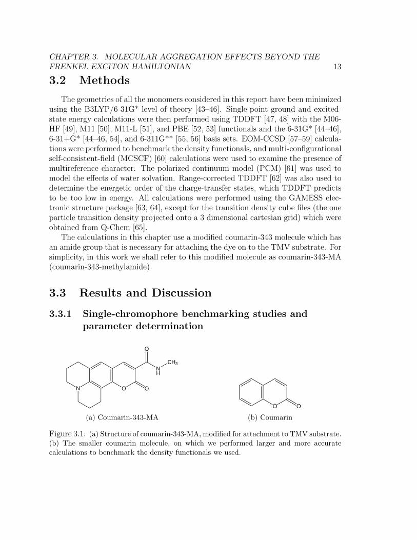
3.1 (a) Structure of coumarin-343-MA, modified for attachment to TMV substrate.
(b) The smaller coumarin molecule, on which we performed larger and more
accurate calculations to benchmark the density functionals we used. . . . . . 133.2 (a) The transition dipole of coumarin-343-MA calculated at the TD-B3LYP/6-
31G* level of theory. (b) The highest occupied molecular orbital (HOMO) of
coumarin-343-MA. (c) The lowest unoccupied molecular orbital (LUMO) of
coumarin-343-MA. . . . . . . . . . . . . . . . . . . . . . . . . . . . . . . . 163.3 Definition and examples of the three angles used to sample the relative orien-
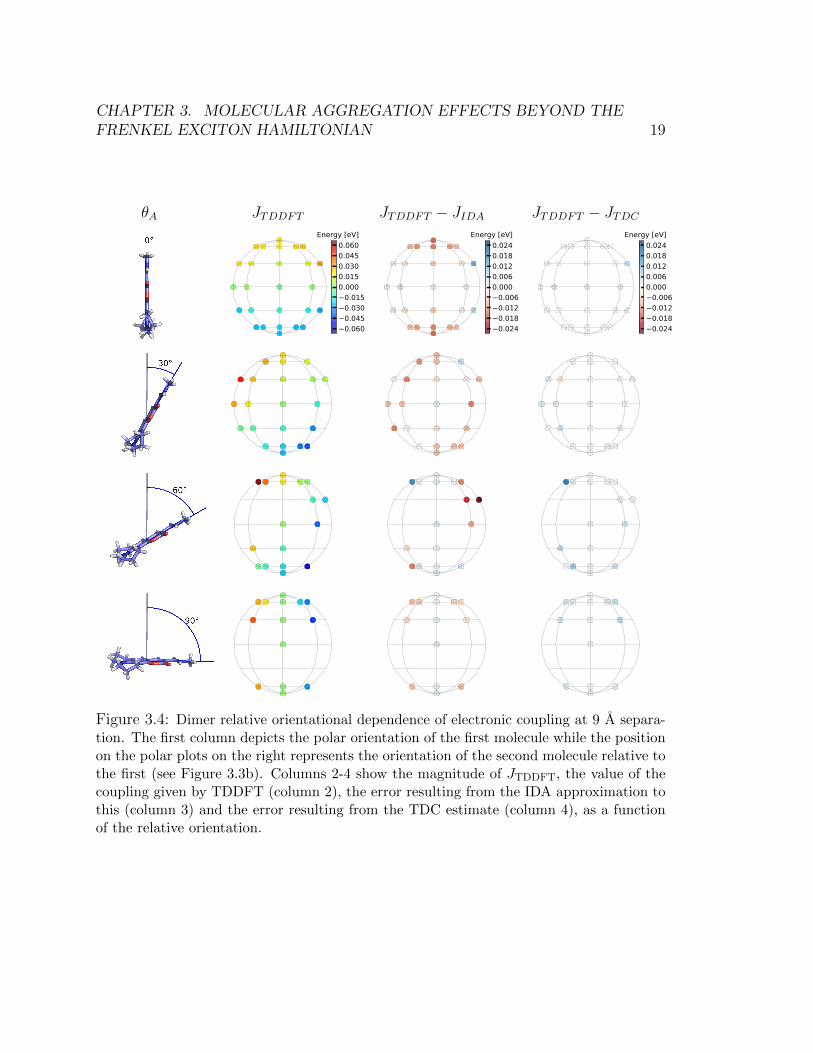
tations between two molecules. . . . . . . . . . . . . . . . . . . . . . . . . 173.4 Dimer relative orientational dependence of electronic coupling at 9 A separa-
tion. The first column depicts the polar orientation of the first molecule while
the position on the polar plots on the right represents the orientation of the
second molecule relative to the first (see Figure 3.3b). Columns 2-4 show the
magnitude of JTDDFT, the value of the coupling given by TDDFT (column 2),
the error resulting from the IDA approximation to this (column 3) and the
error resulting from the TDC estimate (column 4), as a function of the relative
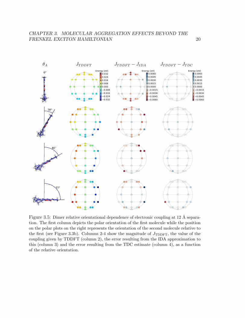
orientation. . . . . . . . . . . . . . . . . . . . . . . . . . . . . . . . . . . . 193.5 Dimer relative orientational dependence of electronic coupling at 12 A separa-
tion. The first column depicts the polar orientation of the first molecule while
the position on the polar plots on the right represents the orientation of the
second molecule relative to the first (see Figure 3.3b). Columns 2-4 show the
magnitude of JTDDFT, the value of the coupling given by TDDFT (column 2),
the error resulting from the IDA approximation to this (column 3) and the
error resulting from the TDC estimate (column 4), as a function of the relative
orientation. . . . . . . . . . . . . . . . . . . . . . . . . . . . . . . . . . . . 20
iv
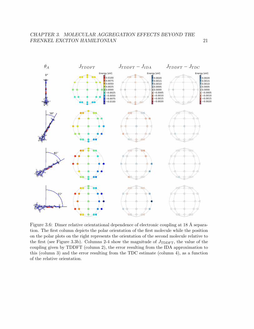
3.6 Dimer relative orientational dependence of electronic coupling at 18 A separa-
tion. The first column depicts the polar orientation of the first molecule while
the position on the polar plots on the right represents the orientation of the
second molecule relative to the first (see Figure 3.3b). Columns 2-4 show the
magnitude of JTDDFT, the value of the coupling given by TDDFT (column 2),
the error resulting from the IDA approximation to this (column 3) and the
error resulting from the TDC estimate (column 4), as a function of the relative
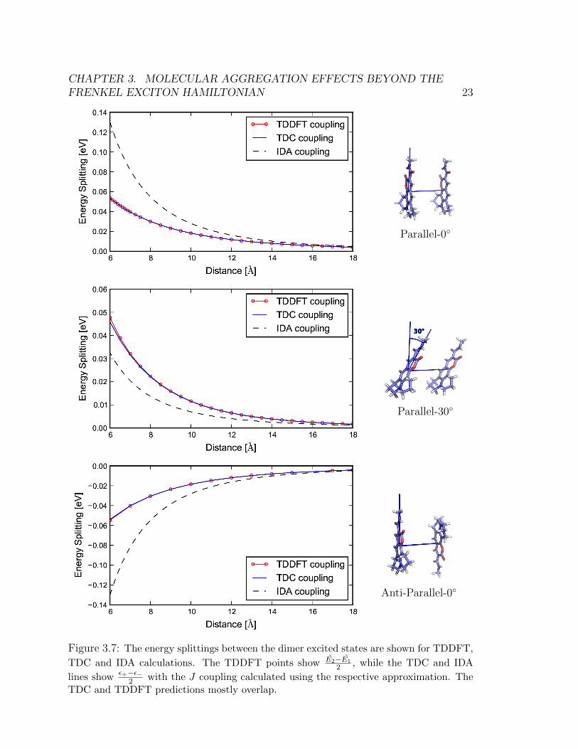
orientation. . . . . . . . . . . . . . . . . . . . . . . . . . . . . . . . . . . . 213.7 The energy splittings between the dimer excited states are shown for TDDFT,
TDC and IDA calculations. The TDDFT points show E2−E12 , while the TDC
and IDA lines show ε+−ε−2 with the J coupling calculated using the respective
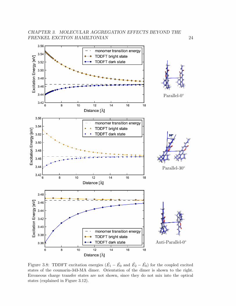
approximation. The TDC and TDDFT predictions mostly overlap. . . . . . 233.8 TDDFT excitation energies (E1 − E0 and E2 − E0) for the coupled excited
states of the coumarin-343-MA dimer. Orientation of the dimer is shown to
the right. Erroneous charge transfer states are not shown, since they do not
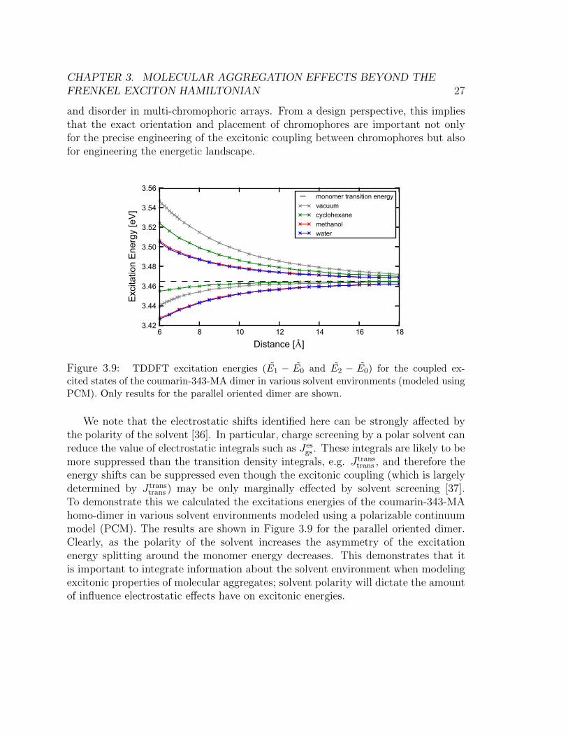
mix into the optical states (explained in Figure 3.12). . . . . . . . . . . . . 243.9 TDDFT excitation energies (E1−E0 and E2−E0) for the coupled excited states
of the coumarin-343-MA dimer in various solvent environments (modeled using
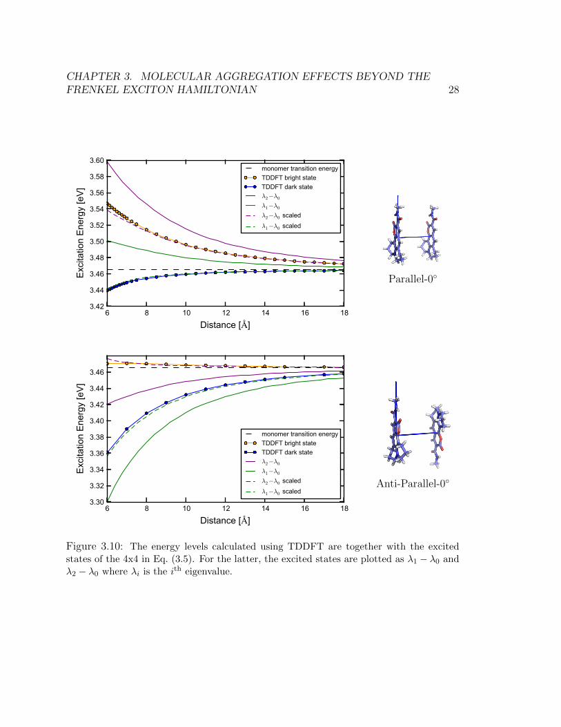
PCM). Only results for the parallel oriented dimer are shown. . . . . . . . . . 273.10 The energy levels calculated using TDDFT are together with the excited states
of the 4x4 in Eq. (3.5). For the latter, the excited states are plotted as λ1−λ0
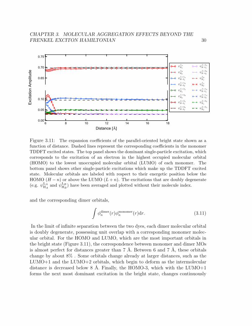
and λ2 − λ0 where λi is the ith eigenvalue. . . . . . . . . . . . . . . . . . . 283.11 The expansion coefficients of the parallel-oriented bright state shown as a func-
tion of distance. Dashed lines represent the corresponding coefficients in the
monomer TDDFT excited states. The top panel shows the dominant single-
particle excitation, which corresponds to the excitation of an electron in the
highest occupied molecular orbital (HOMO) to the lowest unoccupied molec-
ular orbital (LUMO) of each monomer. The bottom panel shows other single-
particle excitations which make up the TDDFT excited state. Molecular or-
bitals are labeled with respect to their energetic position below the HOMO
(H−n) or above the LUMO (L+n). The excitations that are doubly degener-
ate (e.g. ψLAHA
and ψLBHB
) have been averaged and plotted without their molecule
index. . . . . . . . . . . . . . . . . . . . . . . . . . . . . . . . . . . . . . 30
v
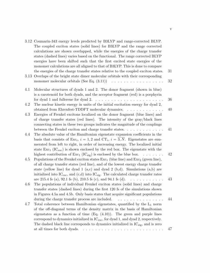
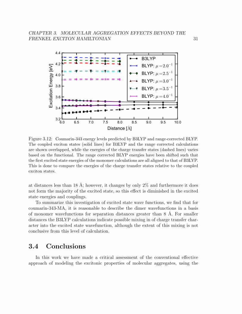
3.12 Coumarin-343 energy levels predicted by B3LYP and range-corrected BLYP.
The coupled exciton states (solid lines) for B3LYP and the range corrected
calculations are shown overlapped, while the energies of the charge transfer
states (dashed lines) varies based on the functional. The range corrected BLYP
energies have been shifted such that the first excited state energies of the
monomer calculations are all aligned to that of B3LYP. This is done to compare
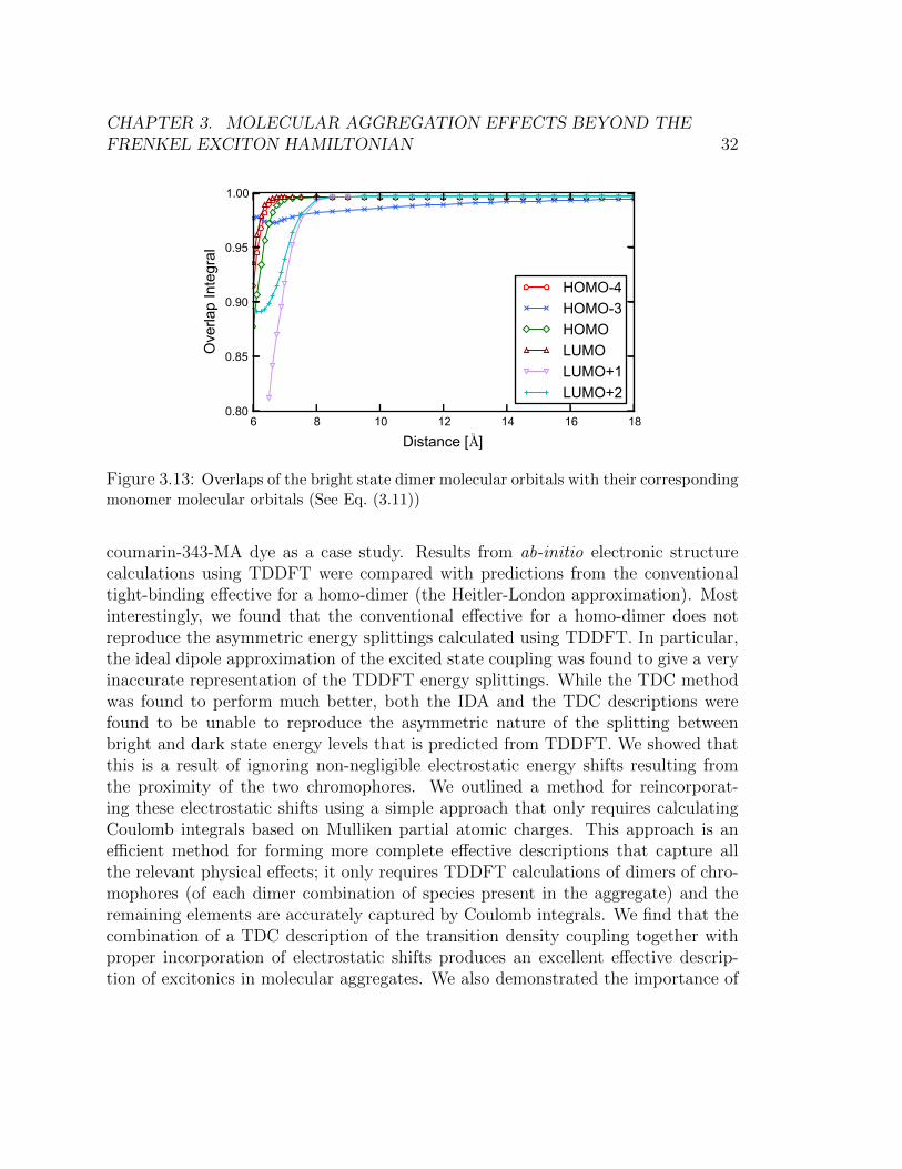
the energies of the charge transfer states relative to the coupled exciton states. 313.13 Overlaps of the bright state dimer molecular orbitals with their corresponding
monomer molecular orbitals (See Eq. (3.11)) . . . . . . . . . . . . . . . . . 32
4.1 Molecular structures of dyads 1 and 2. The donor fragment (shown in blue)
is a carotenoid for both dyads, and the acceptor fragment (red) is a porphyrin
for dyad 1 and fullerene for dyad 2. . . . . . . . . . . . . . . . . . . . . . . 364.2 The nuclear kinetic energy in units of the initial excitation energy for dyad 2,
obtained from Ehrenfest-TDDFT molecular dynamics. . . . . . . . . . . . . 404.3 Energies of Frenkel excitons localized on the donor fragment (blue lines) and
of charge transfer states (red lines). The intensity of the gray/black lines
connecting states in these two groups indicates the magnitude of the couplings
between the Frenkel exciton and charge transfer states. . . . . . . . . . . . . 414.4 The absolute value of the Hamiltonian eigenstate expansion coefficients in the
basis that consists of Exci, i = 1, 2 and CTi, i = 3, N . Eigenstates are enu-
merated from left to right, in order of increasing energy. The localized initial
state Exc1 (ICexc) is shown enclosed by the red box. The eigenstate with the
highest contribution of Exc1 (ICeig) is enclosed by the blue box. . . . . . . . 424.5 Populations of the Frenkel exciton states Exc1 (blue line) and Exc2 (green line),
of all charge transfer states (red line), and of the lowest energy charge transfer
state (yellow line) for dyad 1 (a,c) and dyad 2 (b,d). Simulations (a,b) are
initialized into ICexc, and (c,d) into ICeig. The calculated charge transfer rates
are 215.4 fs (a), 92.1 fs (b), 210.5 fs (c), and 94.1 fs (d). . . . . . . . . . . . 434.6 The populations of individual Frenkel exciton states (solid lines) and charge
transfer states (dashed lines) during the first 120 fs of the simulations shown
in Figures 4.5a and 4.5b. Only basis states that acquire significant populations
during the charge transfer process are included. . . . . . . . . . . . . . . . 444.7 Total coherence between Hamiltonian eigenstates, quantified by the L1 norm
of the off-diagonal terms of the density matrix in the basis of Hamiltonian
eigenstates as a function of time (Eq. (4.10)). The green and purple lines
correspond to dynamics initialized in ICexc, for dyad 1, and dyad 2, respectively.
The dashed black line corresponds to dynamics initialized in ICeig, and is zero
at all times for both dyads. . . . . . . . . . . . . . . . . . . . . . . . . . . 47
vi
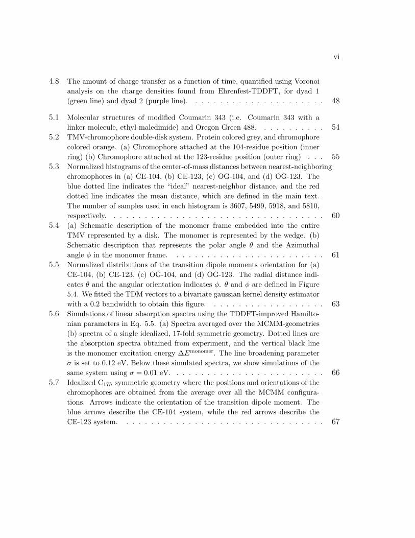
4.8 The amount of charge transfer as a function of time, quantified using Voronoi
analysis on the charge densities found from Ehrenfest-TDDFT, for dyad 1
(green line) and dyad 2 (purple line). . . . . . . . . . . . . . . . . . . . . . 48
5.1 Molecular structures of modified Coumarin 343 (i.e. Coumarin 343 with a
linker molecule, ethyl-maledimide) and Oregon Green 488. . . . . . . . . . . 545.2 TMV-chromophore double-disk system. Protein colored grey, and chromophore
colored orange. (a) Chromophore attached at the 104-residue position (inner
ring) (b) Chromophore attached at the 123-residue position (outer ring) . . . 555.3 Normalized histograms of the center-of-mass distances between nearest-neighboring
chromophores in (a) CE-104, (b) CE-123, (c) OG-104, and (d) OG-123. The
blue dotted line indicates the “ideal” nearest-neighbor distance, and the red
dotted line indicates the mean distance, which are defined in the main text.
The number of samples used in each histogram is 3607, 5499, 5918, and 5810,
respectively. . . . . . . . . . . . . . . . . . . . . . . . . . . . . . . . . . . 605.4 (a) Schematic description of the monomer frame embedded into the entire
TMV represented by a disk. The monomer is represented by the wedge. (b)
Schematic description that represents the polar angle θ and the Azimuthal
angle φ in the monomer frame. . . . . . . . . . . . . . . . . . . . . . . . . 615.5 Normalized distributions of the transition dipole moments orientation for (a)
CE-104, (b) CE-123, (c) OG-104, and (d) OG-123. The radial distance indi-
cates θ and the angular orientation indicates φ. θ and φ are defined in Figure
5.4. We fitted the TDM vectors to a bivariate gaussian kernel density estimator
with a 0.2 bandwidth to obtain this figure. . . . . . . . . . . . . . . . . . . 635.6 Simulations of linear absorption spectra using the TDDFT-improved Hamilto-
nian parameters in Eq. 5.5. (a) Spectra averaged over the MCMM-geometries
(b) spectra of a single idealized, 17-fold symmetric geometry. Dotted lines are
the absorption spectra obtained from experiment, and the vertical black line
is the monomer excitation energy ∆Emonomer. The line broadening parameter
σ is set to 0.12 eV. Below these simulated spectra, we show simulations of the
same system using σ = 0.01 eV. . . . . . . . . . . . . . . . . . . . . . . . . 665.7 Idealized C17h symmetric geometry where the positions and orientations of the
chromophores are obtained from the average over all the MCMM configura-
tions. Arrows indicate the orientation of the transition dipole moment. The
blue arrows describe the CE-104 system, while the red arrows describe the
CE-123 system. . . . . . . . . . . . . . . . . . . . . . . . . . . . . . . . . 67

vii
5.8 The simulated linear absorption spectrum for the MCMM-geometries, using
∆Emonomer1 for all the diagonal energies, and dipole-dipole coupling for the off-
diagonal energies of the Hamiltonian. Refer to Figure 5.6 for an explanation
of the other lines. . . . . . . . . . . . . . . . . . . . . . . . . . . . . . . . 69
viii
List of Tables
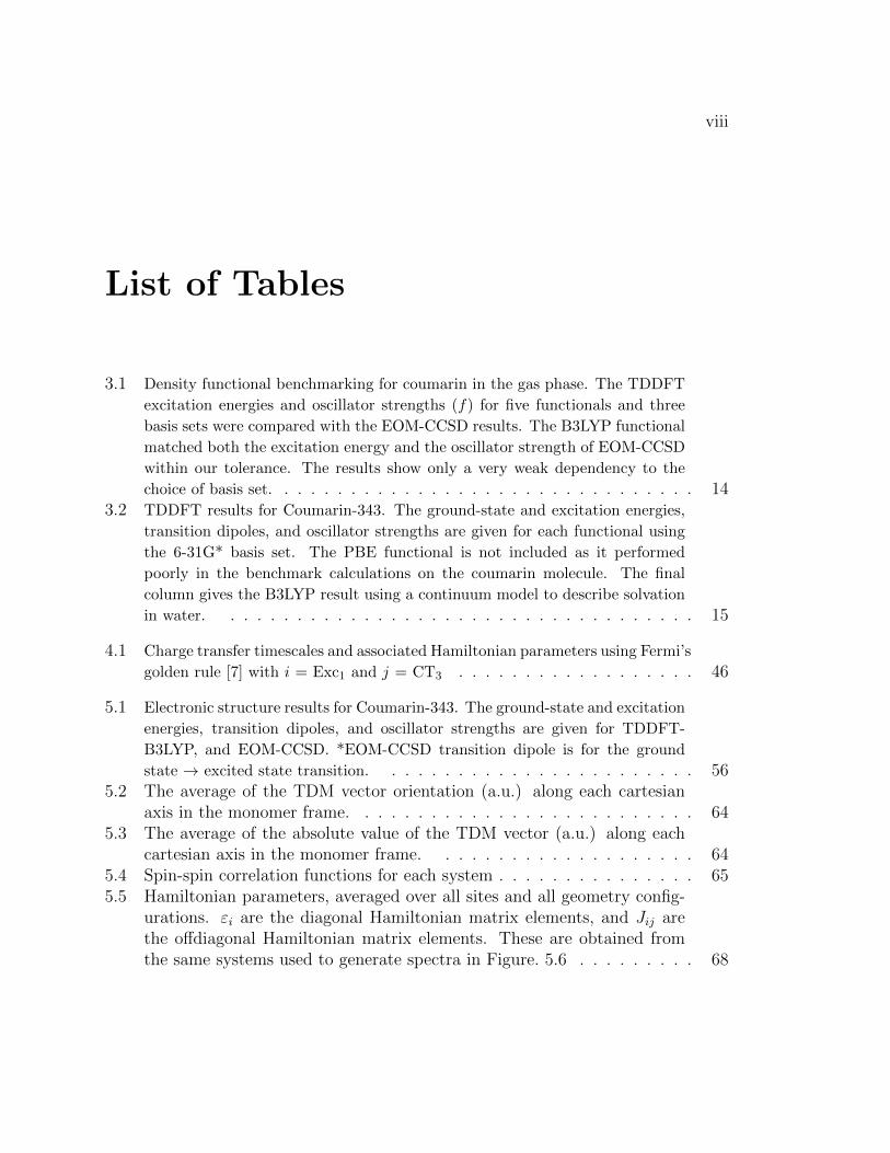
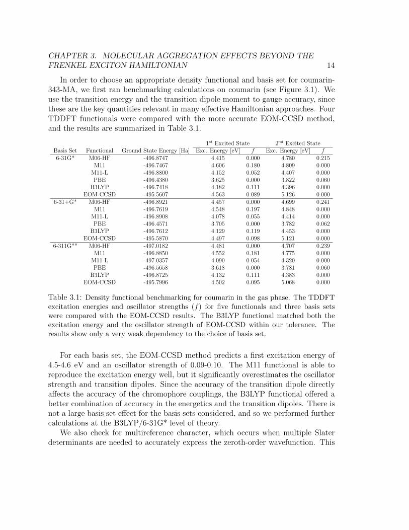
3.1 Density functional benchmarking for coumarin in the gas phase. The TDDFT
excitation energies and oscillator strengths (f) for five functionals and three
basis sets were compared with the EOM-CCSD results. The B3LYP functional
matched both the excitation energy and the oscillator strength of EOM-CCSD
within our tolerance. The results show only a very weak dependency to the
choice of basis set. . . . . . . . . . . . . . . . . . . . . . . . . . . . . . . . 143.2 TDDFT results for Coumarin-343. The ground-state and excitation energies,
transition dipoles, and oscillator strengths are given for each functional using
the 6-31G* basis set. The PBE functional is not included as it performed
poorly in the benchmark calculations on the coumarin molecule. The final
column gives the B3LYP result using a continuum model to describe solvation
in water. . . . . . . . . . . . . . . . . . . . . . . . . . . . . . . . . . . . 15
4.1 Charge transfer timescales and associated Hamiltonian parameters using Fermi’s
golden rule [7] with i = Exc1 and j = CT3 . . . . . . . . . . . . . . . . . . 46
5.1 Electronic structure results for Coumarin-343. The ground-state and excitation
energies, transition dipoles, and oscillator strengths are given for TDDFT-
B3LYP, and EOM-CCSD. *EOM-CCSD transition dipole is for the ground
state → excited state transition. . . . . . . . . . . . . . . . . . . . . . . . 565.2 The average of the TDM vector orientation (a.u.) along each cartesian
axis in the monomer frame. . . . . . . . . . . . . . . . . . . . . . . . . . 645.3 The average of the absolute value of the TDM vector (a.u.) along each
cartesian axis in the monomer frame. . . . . . . . . . . . . . . . . . . . 645.4 Spin-spin correlation functions for each system . . . . . . . . . . . . . . . 655.5 Hamiltonian parameters, averaged over all sites and all geometry config-
urations. εi are the diagonal Hamiltonian matrix elements, and Jij arethe offdiagonal Hamiltonian matrix elements. These are obtained fromthe same systems used to generate spectra in Figure. 5.6 . . . . . . . . . 68

ix
5.6 Average Absorbance. ∆avg is the difference between CE-104 and CE-123average absorbances (λavg
CE-123 − λavgCE-104). . . . . . . . . . . . . . . . . . . . 69

x
Acknowledgments
I would like to first thank my advisor Birgitta Whaley. This work would not havebeen possible without her support and guidance. I would also like to thank thepostdocs Mohan Sarovar, Loren Greenman, and Aleksey Kocherzhenko for their helpand advice, and the other members of the Whaley group for the thought provokingdiscussions that we’ve had. I am also grateful for all of the wonderful people thatI’ve met throughout my journey, and I thank them for their support and friendship.Lastly, I thank my parents Jaemoon and Euna Lee for all of their love and support.

xi
Note on previously published work
The following chapters are adaptions of published papers:
• Chapter 3:Donghyun Lee, Loren Greenman, Mohan Sarovar, and K. Birgitta Whaley“Ab initio calculation of molecular aggregation effects: A coumarin-343 casestudy”Journal of Physical Chemistry A 2013, 117, 11072–11085.http://dx.doi.org/10.1021/jp405152h
• Chapter 4:Donghyun Lee, Michael A. Forsuelo, Aleksey A. Kocherzhenko, and K. BirgittaWhaley“Higher-energy charge transfer states facilitate charge separation in donor-acceptor molecular dyads”Journal of Physical Chemistry C 2017, 121, 13043-13051.http://dx.doi.org/10.1021/acs.jpcc.7b03197
1
Chapter 1
Introduction
Photosynthesis is the quantum mechanical process that provides the energy fornearly all life on earth. The light harvesting stage of photosynthesis begins withthe absorption of a photon by a chromophore, followed by the transport of thiselectronic excitation energy to the reaction center (RC), and finally the separation ofcharges at the RC [1]. While the overall steps in this process are known, there is stillmuch discussion regarding the underlying principles behind these photosyntheticproperties [2–5]. The work described in this thesis is primarily motivated by thedesire to understand the design principles that drives photosynthesis - in particular,how the geometric structure and quantum mechanical properties of chromophoreaggregates affect their electronic and optical properties. In order to do so, it isimportant to begin with a quantum mechanical model that balances efficiency andaccuracy.
1.1 Outline
Motivation
This dissertation is focused on theoretical approaches for predicting the electronicand optical properties of chromophore aggregates. We evaluate the validity of theseapproaches by comparing their predictions to the experimental results obtained fromartificial light-harvesting systems that have been synthesized in lab. In chapter 2,we derive the Frenkel exciton model Hamiltonian from first principles, and note allof the assumptions and approximations used throughout the derivation. In chapter3 we assess the validity of the approximations made in the Frenkel exciton model byexamining the regimes in which the model starts to fail for a chromophore dimer. We
CHAPTER 1. INTRODUCTION 2
introduce a new approach for constructing an improved tight-binding Hamiltonianthat works well at the prototypical intermolecular distances and orientations foundin photosynthetic chromophore aggregates. Chapter 4 describes and evaluates atight-binding Hamiltonian model that treats both electronic excitation transfer andcharge separation together. Chapter 5 introduces a methodology for quantifyingthe geometric disorder in a system, and uses the model in Chapter 3 to simulatelinear absorption spectra. Ultimately, the collection of models presented in thisdissertation provide a framework of theoretical tools for evaluating the electronicand optical properties of real experimental systems, which can be used to screensynthetic candidates for artificial photosynthetic systems.
Chapter 2
The Frenkel exciton model is a tight-binding Hamiltonian that is commonly usedfor modeling chromophore aggregates. Starting from the Born-Oppenheimer molec-ular Hamiltonian, we derive this model while making note of the approximations andassumptions that are used. We state the prerequisite conditions that justifies theseapproximations, and comment on the implications of using these approximations.
Chapter 3
We present time-dependent density functional theory (TDDFT) calculations forsingle and dimerized Coumarin-343 molecules in order to investigate the quantummechanical effects of chromophore aggregation in molecular aggregate systems de-signed to function as artificial light-harvesting devices. Using the single-chromophoreresults, we describe the construction of effective Hamiltonians to predict the excitonicproperties of aggregate systems. We compare the electronic coupling properties pre-dicted by such effective Hamiltonians to those obtained from TDDFT calculations ofdimers, and to the coupling predicted by the transition density cube (TDC) method.We determine the accuracy of the dipole-dipole approximation and TDC with respectto the separation distance and orientation of the dimers. In particular, we investigatethe effects of including Coulomb coupling terms ignored in the Frenkel exciton tight-binding Hamiltonian. We also examine effects of orbital relaxation which cannot becaptured by either of these models.
Chapter 4
We simulate sub-picosecond charge separation in two donor-acceptor moleculardyads where it has previously been observed experimentally [6]. Charge separation
CHAPTER 1. INTRODUCTION 3
dynamics is described using a quantum master equation, with parameters of the dyadHamiltonian obtained from density functional theory (DFT) and time-dependentdensity functional theory (TDDFT) calculations, and the rate of energy dissipationestimated from Ehrenfest-TDDFT molecular dynamics simulations. We find thathigher energy charge transfer states must be included in the dyad Hamiltonian inorder to obtain agreement of charge separation rates with the experimental values.Golden rule rate constants are found to be inadequate. Our results show that efficientand irreversible charge separation involves both coherent electron transfer from thedonor excited state to higher energy unoccupied states on the acceptor and incoherentenergy dissipation that relaxes the dyad to the lowest energy charge transfer state.The role of coherence depends on the initial excited state, with electron delocalizationwithin Hamiltonian eigenstates found to be more important than coherence betweeneigenstates. We conclude that ultrafast charge separation is most likely to occur indonor-acceptor dyads possessing dense manifolds of charge transfer states at energiesclose to those of Frenkel excitons on the donor, with strong couplings to these statesenabling partial delocalization of eigenstates over acceptor and donor.
Chapter 5
We present molecular mechanics calculations on a prototype artificial light har-vesting system consisting of chromophores attached to a tobacco mosaic virus (TMV)protein scaffold. These systems have been synthesized and characterized spectro-scopically, but information about the microscopic configurations and geometry ofthese TMV-templated chromophore assemblies is largely unknown. We use a MonteCarlo conformational search algorithm to determine the preferred positions and ori-entations of two chromophores, Coumarin 343 together with its linker, and OregonGreen 488, when these are attached at two different sites (104 and 123) on the TMVprotein. The resulting geometric information shows that the extent of disorder andaggregation properties, and therefore the optical properties of the TMV-templatedchromophore assembly, are highly dependent on the choice of chromophores and pro-tein site to which they are bound. We used the results of the conformational searchas geometric parameters together with an improved tight-binding Hamiltonian tosimulate the linear absorption spectra and compare with experimental spectral mea-surements. We found that using the geometries from the conformational search isnecessary to reproduce qualitative features of the experimental spectral peaks.

CHAPTER 1. INTRODUCTION 4
Chapter 6
We summarize the techniques for modeling chromophore aggregates that havebeen introduced in this thesis, and discuss some of the design principles for creatingartificial photosynthetic systems that have been elucidated by using these techniques.We propose some topics of future research that would be interesting to investigateas an extension to the work in this thesis.
5
Chapter 2
Frenkel Exciton Hamiltonian
2.1 Molecular Hamiltonian
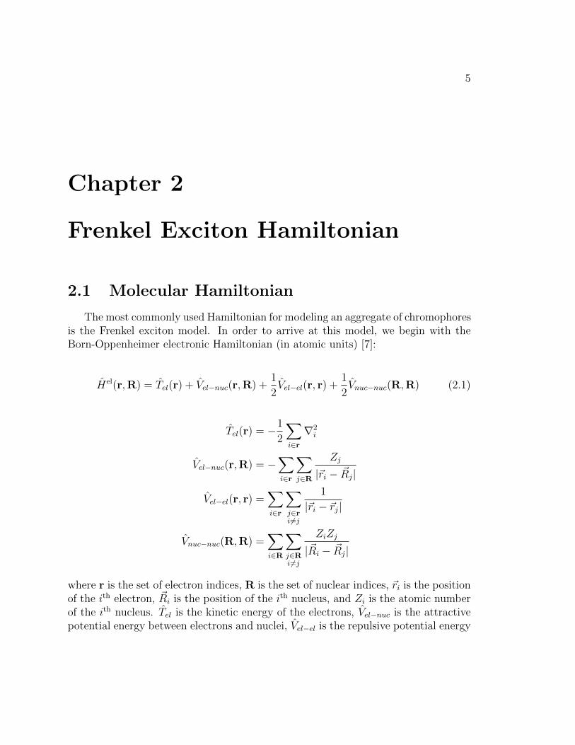
The most commonly used Hamiltonian for modeling an aggregate of chromophoresis the Frenkel exciton model. In order to arrive at this model, we begin with theBorn-Oppenheimer electronic Hamiltonian (in atomic units) [7]:
Hel(r,R) = Tel(r) + Vel−nuc(r,R) +1
2Vel−el(r, r) +
1
2Vnuc−nuc(R,R) (2.1)
Tel(r) = −1
2
∑i∈r
∇2i
Vel−nuc(r,R) = −∑i∈r
∑j∈R
Zj
|~ri − ~Rj|
Vel−el(r, r) =∑i∈r
∑j∈ri 6=j
1
|~ri − ~rj|
Vnuc−nuc(R,R) =∑i∈R
∑j∈Ri 6=j
ZiZj
|~Ri − ~Rj|
where r is the set of electron indices, R is the set of nuclear indices, ~ri is the positionof the ith electron, ~Ri is the position of the ith nucleus, and Zi is the atomic numberof the ith nucleus. Tel is the kinetic energy of the electrons, Vel−nuc is the attractivepotential energy between electrons and nuclei, Vel−el is the repulsive potential energy
CHAPTER 2. FRENKEL EXCITON HAMILTONIAN 6
between electrons, and Vnuc−nuc is the repulsive potential energy between nuclei. Thisis the Hamiltonian over the electronic degrees of freedom, with respect to a fixed setof nuclear coordinates.
2.2 Frenkel Exciton Model
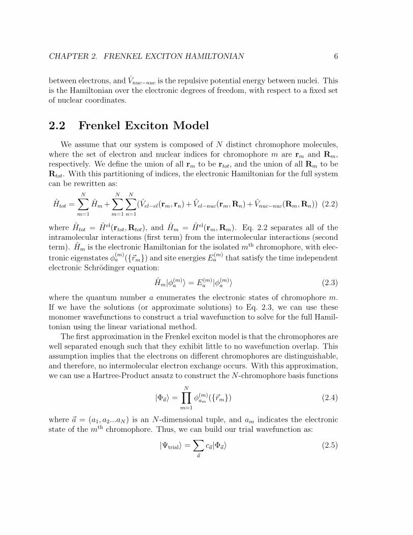
We assume that our system is composed of N distinct chromophore molecules,where the set of electron and nuclear indices for chromophore m are rm and Rm,respectively. We define the union of all rm to be rtot, and the union of all Rm to beRtot. With this partitioning of indices, the electronic Hamiltonian for the full systemcan be rewritten as:
Htot =N∑m=1
Hm +N∑m=1
N∑n=1
(Vel−el(rm, rn) + Vel−nuc(rm,Rn) + Vnuc−nuc(Rm,Rn)) (2.2)
where Htot = Hel(rtot,Rtot), and Hm = Hel(rm,Rm). Eq. 2.2 separates all of theintramolecular interactions (first term) from the intermolecular interactions (secondterm). Hm is the electronic Hamiltonian for the isolated mth chromophore, with elec-
tronic eigenstates φ(m)a ({~rm}) and site energies E
(m)a that satisfy the time independent
electronic Schrodinger equation:
Hm|φ(m)a 〉 = E(m)
a |φ(m)a 〉 (2.3)
where the quantum number a enumerates the electronic states of chromophore m.If we have the solutions (or approximate solutions) to Eq. 2.3, we can use thesemonomer wavefunctions to construct a trial wavefunction to solve for the full Hamil-tonian using the linear variational method.
The first approximation in the Frenkel exciton model is that the chromophores arewell separated enough such that they exhibit little to no wavefunction overlap. Thisassumption implies that the electrons on different chromophores are distinguishable,and therefore, no intermolecular electron exchange occurs. With this approximation,we can use a Hartree-Product ansatz to construct the N -chromophore basis functions
|Φ~a〉 =N∏m=1
φ(m)am ({~rm}) (2.4)
where ~a = (a1, a2...aN) is an N -dimensional tuple, and am indicates the electronicstate of the mth chromophore. Thus, we can build our trial wavefunction as:
|Ψtrial〉 =∑~a
c~a|Φ~a〉 (2.5)
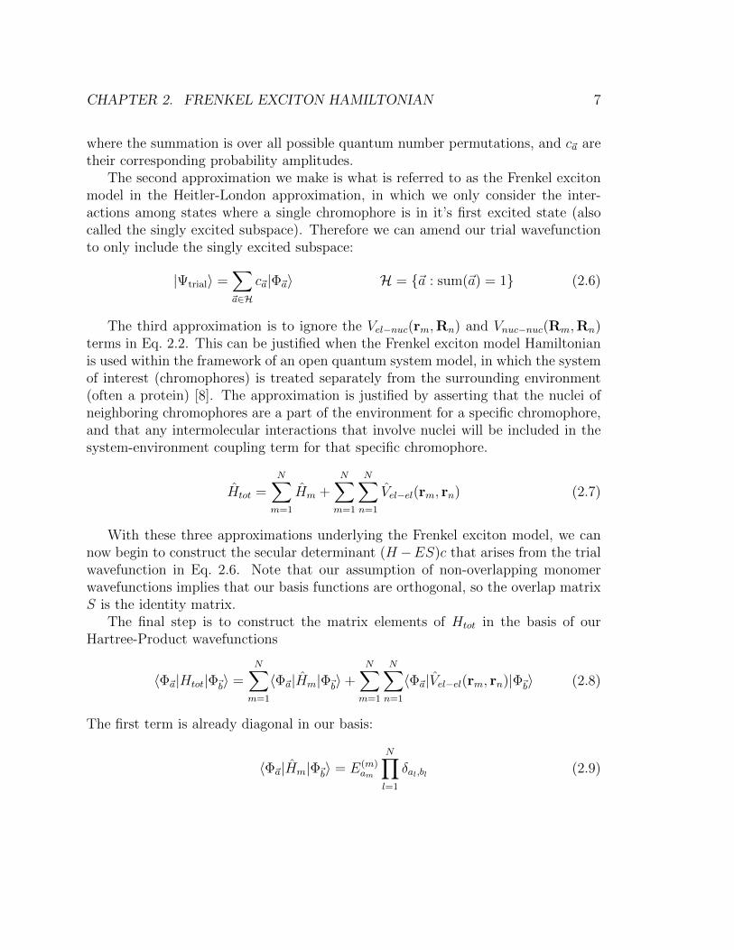
CHAPTER 2. FRENKEL EXCITON HAMILTONIAN 7
where the summation is over all possible quantum number permutations, and c~a aretheir corresponding probability amplitudes.
The second approximation we make is what is referred to as the Frenkel excitonmodel in the Heitler-London approximation, in which we only consider the inter-actions among states where a single chromophore is in it’s first excited state (alsocalled the singly excited subspace). Therefore we can amend our trial wavefunctionto only include the singly excited subspace:
|Ψtrial〉 =∑~a∈H
c~a|Φ~a〉 H = {~a : sum(~a) = 1} (2.6)
The third approximation is to ignore the Vel−nuc(rm,Rn) and Vnuc−nuc(Rm,Rn)terms in Eq. 2.2. This can be justified when the Frenkel exciton model Hamiltonianis used within the framework of an open quantum system model, in which the systemof interest (chromophores) is treated separately from the surrounding environment(often a protein) [8]. The approximation is justified by asserting that the nuclei ofneighboring chromophores are a part of the environment for a specific chromophore,and that any intermolecular interactions that involve nuclei will be included in thesystem-environment coupling term for that specific chromophore.
Htot =N∑m=1
Hm +N∑m=1
N∑n=1
Vel−el(rm, rn) (2.7)
With these three approximations underlying the Frenkel exciton model, we cannow begin to construct the secular determinant (H −ES)c that arises from the trialwavefunction in Eq. 2.6. Note that our assumption of non-overlapping monomerwavefunctions implies that our basis functions are orthogonal, so the overlap matrixS is the identity matrix.
The final step is to construct the matrix elements of Htot in the basis of ourHartree-Product wavefunctions
〈Φ~a|Htot|Φ~b〉 =N∑m=1
〈Φ~a|Hm|Φ~b〉+N∑m=1
N∑n=1
〈Φ~a|Vel−el(rm, rn)|Φ~b〉 (2.8)
The first term is already diagonal in our basis:
〈Φ~a|Hm|Φ~b〉 = E(m)am
N∏l=1
δal,bl (2.9)
CHAPTER 2. FRENKEL EXCITON HAMILTONIAN 8
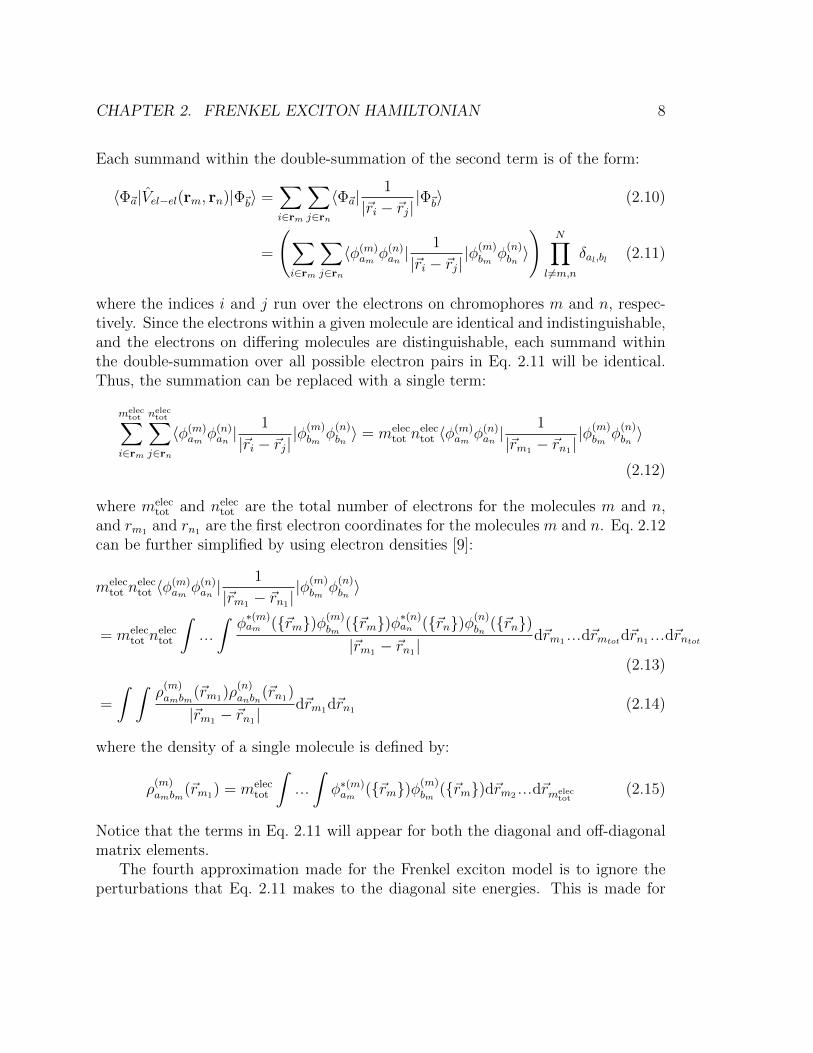
Each summand within the double-summation of the second term is of the form:
〈Φ~a|Vel−el(rm, rn)|Φ~b〉 =∑i∈rm
∑j∈rn
〈Φ~a|1
|~ri − ~rj||Φ~b〉 (2.10)
=
(∑i∈rm
∑j∈rn
〈φ(m)am φ
(n)an |
1
|~ri − ~rj||φ(m)bmφ
(n)bn〉
)N∏
l 6=m,n
δal,bl (2.11)
where the indices i and j run over the electrons on chromophores m and n, respec-tively. Since the electrons within a given molecule are identical and indistinguishable,and the electrons on differing molecules are distinguishable, each summand withinthe double-summation over all possible electron pairs in Eq. 2.11 will be identical.Thus, the summation can be replaced with a single term:
melectot∑
i∈rm
nelectot∑
j∈rn
〈φ(m)am φ
(n)an |
1
|~ri − ~rj||φ(m)bmφ
(n)bn〉 = melec
tot nelectot 〈φ(m)
am φ(n)an |
1
|~rm1 − ~rn1||φ(m)bmφ
(n)bn〉
(2.12)
where melectot and nelec
tot are the total number of electrons for the molecules m and n,and rm1 and rn1 are the first electron coordinates for the molecules m and n. Eq. 2.12can be further simplified by using electron densities [9]:
melectot n
electot 〈φ(m)
am φ(n)an |
1
|~rm1 − ~rn1||φ(m)bmφ
(n)bn〉
= melectot n
electot
∫...
∫φ∗(m)am ({~rm})φ(m)
bm({~rm})φ∗(n)
an ({~rn})φ(n)bn
({~rn})|~rm1 − ~rn1|
d~rm1 ...d~rmtotd~rn1 ...d~rntot
(2.13)
=
∫ ∫ρ
(m)ambm
(~rm1)ρ(n)anbn
(~rn1)
|~rm1 − ~rn1|d~rm1d~rn1 (2.14)
where the density of a single molecule is defined by:
ρ(m)ambm
(~rm1) = melectot
∫...
∫φ∗(m)am ({~rm})φ(m)
bm({~rm})d~rm2 ...d~rmelec
tot(2.15)
Notice that the terms in Eq. 2.11 will appear for both the diagonal and off-diagonalmatrix elements.
The fourth approximation made for the Frenkel exciton model is to ignore theperturbations that Eq. 2.11 makes to the diagonal site energies. This is made for
CHAPTER 2. FRENKEL EXCITON HAMILTONIAN 9
a similar reason as the third approximation - namely any perturbations to the siteenergies will be captured by the system-environment coupling terms.
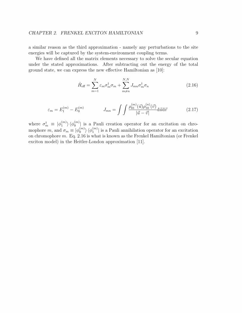
We have defined all the matrix elements necessary to solve the secular equationunder the stated approximations. After subtracting out the energy of the totalground state, we can express the new effective Hamiltonian as [10]:
Heff =N∑m=1
εmσ†mσm +
N,N∑m6=n
Jmnσ†mσn (2.16)
εm = E(m)1 − E(m)
0 Jmn =
∫ ∫ρ
(m)01 (~u)ρ
(n)10 (~v)
|~u− ~v|d~ud~v (2.17)
where σ†m ≡ |φ(m)1 〉 〈φ
(m)0 | is a Pauli creation operator for an excitation on chro-
mophore m, and σm ≡ |φ(m)0 〉 〈φ
(m)1 | is a Pauli annihilation operator for an excitation
on chromophore m. Eq. 2.16 is what is known as the Frenkel Hamiltonian (or Frenkelexciton model) in the Heitler-London approximation [11].
10
Chapter 3
Molecular aggregation effectsbeyond the Frenkel ExcitonHamiltonian
3.1 Introduction
The geometry of chromophore aggregates influences how they couple to one an-other, which in turn determines the electronic properties of the extended system.Deliberate control over the positions and orientations of chromophores can therebybe used to achieve specific properties such as efficient energy transfer [12]. Light har-vesting in photosynthesis is an example from nature of how chromophores embeddedin proteins have been optimized by evolution to capture light over a specific spec-trum and to efficiently transfer the excitation energy to the photosynthetic reactioncenter [1, 5, 13, 14]. In designing synthetic light harvesting antennae for organic sen-sors or photovoltaics, it is critical to understand how the structural and orientationalproperties of the chromophore arrays affects their coupling, and hence their excitonicand optical properties [9, 15–19]. Importantly, recent work has suggested that quan-tum mechanical effects play a key role in the high efficiency of biological excitationenergy transfer (EET) [3, 20–22]. Understanding the details of the quantum me-chanical coupling between chromophores is an important step towards probing andexploiting any beneficial effects of quantum mechanical coherence in energy transfer.
Due to its spectroscopic attributes and small size, coumarin-343 (see Figure 3.1)is a molecule of particular interest for use in virus-templated synthetic light har-vesting complexes, using e.g. the tobacco mosaic virus (TMV) protein scaffold [23].The TMV protein monomers undergo self-assembly to form complex structures such
CHAPTER 3. MOLECULAR AGGREGATION EFFECTS BEYOND THEFRENKEL EXCITON HAMILTONIAN 11
as helices and stacked disks [24]. The assembled TMV can be made into a lightharvesting array by covalently attaching chromophores such as coumarin-343 ontothe protein [23, 25–27]. The stacked disks and helical arrays of chromophores actas aggregate systems with optical properties (spectral width, peak absorption fre-quency) that differ from those of the free chromophore. It is possible to exercise afine degree of control over these optical properties by changing the concentration ofchromophores and the positions at which they are attached [28].
Conventionally the interaction between excited states of nearby chromophores ismodeled using a tight-binding Hamiltonian of the form [14, 29],
H =N∑i=1
εiσ†iσi +
N,N∑i 6=j
Ji,jσ†iσj, (3.1)
where εi is the transition energy of chromophore i, Ji,j is the coupling between chro-
mophores i and j, σ†i ≡ |ψi1〉 〈ψi0| is a Pauli creation operator for an excitation onchromophore i, and σi ≡ |ψi0〉 〈ψi1| is a Pauli annihilation operator for an excita-tion on chromophore i. In this approach each molecule is treated as a two-levelsystem and the number of excitations is conserved. This truncated description ofthe intermolecular Hamiltonian is often referred to as the Frenkel Hamiltonian (orFrenkel exciton model) in the Heitler-London approximation [11]. Such effectiveHamiltonian descriptions constitute the only feasible approach to study large molec-ular aggregates, since ab-initio methods cannot be scaled to such large systems.However, some of the parameters entering the effective Hamiltonian descriptions canbe calculated using ab-initio methods. For instance, the coupling between chro-mophores (Ji,j), which is well-approximated by a Coulombic interaction between thetransition densities of chromophores i and j, can be calculated exactly using thetransition density cube (TDC) method [30]. The most common way to approximatethis coupling is by the ideal dipole approximation (IDA) [31] which treats the 1/rinteraction between the two densities as an interaction between the dipole momentsof the transition densities; several papers have compared the accuracy of the IDAto the more complete TDC description in various molecules [32–34]. The effectiveHamiltonian in Eq. (3.1) relies on the approximation that the aggregate wavefunc-tion can be reasonably constructed from the product of monomer wavefunctions (aHeitler-London-type picture). However such effective Hamiltonian descriptions mayalso neglect other potentially important aspects of the intermolecular interactions. Inparticular, Eq. (3.1) does not include electron exchange between the chromophores,nor does it allow for relaxation of the monomer wavefunctions. To go beyond thisapproximate description requires making detailed electronic structure calculationson the aggregate, and this is what we undertake in this study.
CHAPTER 3. MOLECULAR AGGREGATION EFFECTS BEYOND THEFRENKEL EXCITON HAMILTONIAN 12
In the following sections we present time-dependent density functional theory(TDDFT) results for coumarin-343 and compare them to results from the IDA andTDC. We also compare to an effective Hamiltonian that we obtain from expressingthe molecular Hamiltonian in a basis constructed from products of monomer wave-functions. TDDFT provides a middle ground between accuracy and computationalexpense, and we have performed some benchmarking calculations to determine thequality of TDDFT for coumarin.
The results presented here are similar in spirit to a number of recent ab-initiostudies of excited states of molecular aggregates, and we briefly review some ofthese studies here. Firstly, Ref. [35], which perhaps has the most overlap with theresults in this work, develops a method referred to as TrEsp for using ab-initio cal-culations of charge and transition densities for monomers to determine energies ofexcited states of coupled chromophores. Next, some recent papers, e.g., [36, 37],have examined the various components of electronic coupling in condensed mediausing ab-initio methods, separately characterized through-bond and through-spacecontributions, and analyzed the effects of solvent properties on these. Finally, severalworks have examined the aggregation mechanisms and subsequent excited states ofmolecular aggregates of dimers and extended systems using ab-initio methods [38–42]. These studies concentrate on aggregates common in molecular crystals (e.g.,perylene bisimide (PBI) aggregates) and as a result focus on very densely packedsystems; typical inter-molecular separation distances studied in these works are inthe range 2-8A. In such self-assembling aggregates the mechanisms that dictate aggre-gation geometries and intermolecular potentials – e.g., dispersion forces – are criticalto understanding excited state energies. In contrast, in the papers cited above andin this work the focus is on molecular aggregates found in biomimetic or biologicalsystems. In such systems the inter-molecular separation is typically larger, and crit-ically, the forces that dictate aggregation are mostly due to external influences suchas protein scaffolds. Therefore in such systems the intermolecular potentials play asmaller role although as we show below they cannot be ignored completely.
An outline of the remainder of this chapter follows. In section 3.3.1, we presentthese benchmarking calculations and give the TDDFT transition energies and transi-tion dipoles for a single coumarin-343 chromophore. These are the simplest parame-ters which can be used in Eq. (3.1). Then, in section 3.3.2, we explore using TDDFTthe energetics resulting from coupling between two dyes at a number of separationdistances and orientations. We compare the TDDFT exciton splitting energies tosplittings calculated by approximate methods, and also examine the effects of ag-gregation on exciton energies and wave functions, in particular, the role of orbitalrelaxation and deviations from the solutions to the Heitler-London description ofmonomer coupling.
CHAPTER 3. MOLECULAR AGGREGATION EFFECTS BEYOND THEFRENKEL EXCITON HAMILTONIAN 13
3.2 Methods
The geometries of all the monomers considered in this report have been minimizedusing the B3LYP/6-31G* level of theory [43–46]. Single-point ground and excited-state energy calculations were then performed using TDDFT [47, 48] with the M06-HF [49], M11 [50], M11-L [51], and PBE [52, 53] functionals and the 6-31G* [44–46],6-31+G* [44–46, 54], and 6-311G** [55, 56] basis sets. EOM-CCSD [57–59] calcula-tions were performed to benchmark the density functionals, and multi-configurationalself-consistent-field (MCSCF) [60] calculations were used to examine the presence ofmultireference character. The polarized continuum model (PCM) [61] was used tomodel the effects of water solvation. Range-corrected TDDFT [62] was also used todetermine the energetic order of the charge-transfer states, which TDDFT predictsto be too low in energy. All calculations were performed using the GAMESS elec-tronic structure package [63, 64], except for the transition density cube files (the oneparticle transition density projected onto a 3 dimensional cartesian grid) which wereobtained from Q-Chem [65].
The calculations in this chapter use a modified coumarin-343 molecule which hasan amide group that is necessary for attaching the dye on to the TMV substrate. Forsimplicity, in this work we shall refer to this modified molecule as coumarin-343-MA(coumarin-343-methylamide).
3.3 Results and Discussion
3.3.1 Single-chromophore benchmarking studies andparameter determination
O ON
NH
O
CH3
(a) Coumarin-343-MA
O O
(b) Coumarin
Figure 3.1: (a) Structure of coumarin-343-MA, modified for attachment to TMV substrate.(b) The smaller coumarin molecule, on which we performed larger and more accuratecalculations to benchmark the density functionals we used.
CHAPTER 3. MOLECULAR AGGREGATION EFFECTS BEYOND THEFRENKEL EXCITON HAMILTONIAN 14
In order to choose an appropriate density functional and basis set for coumarin-343-MA, we first ran benchmarking calculations on coumarin (see Figure 3.1). Weuse the transition energy and the transition dipole moment to gauge accuracy, sincethese are the key quantities relevant in many effective Hamiltonian approaches. FourTDDFT functionals were compared with the more accurate EOM-CCSD method,and the results are summarized in Table 3.1.
1st Excited State 2nd Excited StateBasis Set Functional Ground State Energy [Ha] Exc. Energy [eV] f Exc. Energy [eV] f6-31G* M06-HF -496.8747 4.415 0.000 4.780 0.215
M11 -496.7467 4.606 0.180 4.809 0.000M11-L -496.8800 4.152 0.052 4.407 0.000PBE -496.4380 3.625 0.000 3.822 0.060
B3LYP -496.7418 4.182 0.111 4.396 0.000EOM-CCSD -495.5607 4.563 0.089 5.126 0.000
6-31+G* M06-HF -496.8921 4.457 0.000 4.699 0.241M11 -496.7619 4.548 0.197 4.848 0.000
M11-L -496.8908 4.078 0.055 4.414 0.000PBE -496.4571 3.705 0.000 3.782 0.062
B3LYP -496.7612 4.129 0.119 4.453 0.000EOM-CCSD -495.5870 4.497 0.098 5.121 0.000
6-311G** M06-HF -497.0182 4.481 0.000 4.707 0.239M11 -496.8850 4.552 0.181 4.775 0.000
M11-L -497.0357 4.090 0.054 4.320 0.000PBE -496.5658 3.618 0.000 3.781 0.060
B3LYP -496.8725 4.132 0.111 4.383 0.000EOM-CCSD -495.7996 4.502 0.095 5.068 0.000
Table 3.1: Density functional benchmarking for coumarin in the gas phase. The TDDFTexcitation energies and oscillator strengths (f) for five functionals and three basis setswere compared with the EOM-CCSD results. The B3LYP functional matched both theexcitation energy and the oscillator strength of EOM-CCSD within our tolerance. Theresults show only a very weak dependency to the choice of basis set.
For each basis set, the EOM-CCSD method predicts a first excitation energy of4.5-4.6 eV and an oscillator strength of 0.09-0.10. The M11 functional is able toreproduce the excitation energy well, but it significantly overestimates the oscillatorstrength and transition dipoles. Since the accuracy of the transition dipole directlyaffects the accuracy of the chromophore couplings, the B3LYP functional offered abetter combination of accuracy in the energetics and the transition dipoles. There isnot a large basis set effect for the basis sets considered, and so we performed furthercalculations at the B3LYP/6-31G* level of theory.
We also check for multireference character, which occurs when multiple Slaterdeterminants are needed to accurately express the zeroth-order wavefunction. This
CHAPTER 3. MOLECULAR AGGREGATION EFFECTS BEYOND THEFRENKEL EXCITON HAMILTONIAN 15
is common for large or conjugated molecules. MCSCF calculations were run oncoumarin-343-MA using an active space of 7 electrons in 7 π-orbitals. The naturalorbital occupation numbers, which are the eigenvalues of the one-electron reduceddensity operator [66],
γ(r1, r′1) = N
∫· · ·∫ψ∗(r1, r2 . . . rN)ψ(r′1, r2 . . . rN)dr2 . . . drN , (3.2)
are useful for determining multireference character; occupation numbers that deviatesignificantly from 0.0 or 2.0 indicate that a multireference wavefunction is needed.We find that the occupation numbers of the occupied and unoccupied orbitals wereall greater than 1.9 or less than 0.12. This indicates that there is little multireferencecharacter for this dye and so the benchmark calculations and TDDFT calculationsare both adequate.
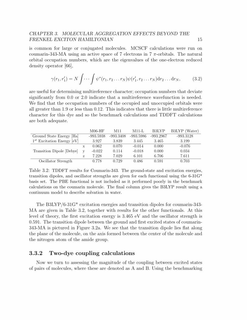
M06-HF M11 M11-L B3LYP B3LYP (Water)Ground State Energy [Ha] -993.5938 -993.3408 -993.5986 -993.2967 -993.31281st Excitation Energy [eV] 3.927 3.839 3.445 3.465 3.199
x 0.062 0.070 -0.014 0.000 -0.076Transition Dipole [Debye] y -0.022 0.114 -0.018 0.000 0.034
z 7.228 7.029 6.101 6.706 7.611Oscillator Strength 0.778 0.729 0.486 0.591 0.703
Table 3.2: TDDFT results for Coumarin-343. The ground-state and excitation energies,transition dipoles, and oscillator strengths are given for each functional using the 6-31G*basis set. The PBE functional is not included as it performed poorly in the benchmarkcalculations on the coumarin molecule. The final column gives the B3LYP result using acontinuum model to describe solvation in water.
The B3LYP/6-31G* excitation energies and transition dipoles for coumarin-343-MA are given in Table 3.2, together with results for the other functionals. At thislevel of theory, the first excitation energy is 3.465 eV and the oscillator strength is0.591. The transition dipole between the ground and first excited states of coumarin-343-MA is pictured in Figure 3.2a. We see that the transition dipole lies flat alongthe plane of the molecule, on the axis formed between the center of the molecule andthe nitrogen atom of the amide group.
3.3.2 Two-dye coupling calculations
Now we turn to assessing the magnitude of the coupling between excited statesof pairs of molecules, where these are denoted as A and B. Using the benchmarking
CHAPTER 3. MOLECULAR AGGREGATION EFFECTS BEYOND THEFRENKEL EXCITON HAMILTONIAN 16
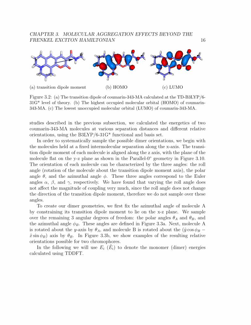
(a) transition dipole moment (b) HOMO (c) LUMO
Figure 3.2: (a) The transition dipole of coumarin-343-MA calculated at the TD-B3LYP/6-31G* level of theory. (b) The highest occupied molecular orbital (HOMO) of coumarin-343-MA. (c) The lowest unoccupied molecular orbital (LUMO) of coumarin-343-MA.
studies described in the previous subsection, we calculated the energetics of twocoumarin-343-MA molecules at various separation distances and different relativeorientations, using the B3LYP/6-31G* functional and basis set.
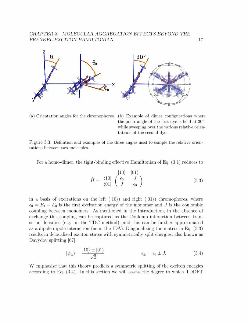
In order to systematically sample the possible dimer orientations, we begin withthe molecules held at a fixed intermolecular separation along the x-axis. The transi-tion dipole moment of each molecule is aligned along the z axis, with the plane of themolecule flat on the y-z plane as shown in the Parallel-0◦ geometry in Figure 3.10.The orientation of each molecule can be characterized by the three angles: the rollangle (rotation of the molecule about the transition dipole moment axis), the polarangle θ, and the azimuthal angle φ. These three angles correspond to the Eulerangles α, β, and γ, respectively. We have found that varying the roll angle doesnot affect the magnitude of coupling very much, since the roll angle does not changethe direction of the transition dipole moment, therefore we do not sample over theseangles.
To create our dimer geometries, we first fix the azimuthal angle of molecule Aby constraining its transition dipole moment to lie on the x-z plane. We sampleover the remaining 3 angular degrees of freedom: the polar angles θA and θB, andthe azimuthal angle φB. These angles are defined in Figure 3.3a. Next, molecule Ais rotated about the y-axis by θA, and molecule B is rotated about the (y cosφB −x sinφB) axis by θB. In Figure 3.3b, we show examples of the resulting relativeorientations possible for two chromophores.
In the following we will use Ei (Ei) to denote the monomer (dimer) energiescalculated using TDDFT.
CHAPTER 3. MOLECULAR AGGREGATION EFFECTS BEYOND THEFRENKEL EXCITON HAMILTONIAN 17
(a) Orientation angles for the chromophores. (b) Example of dimer configurations wherethe polar angle of the first dye is held at 30◦,while sweeping over the various relative orien-tations of the second dye.
Figure 3.3: Definition and examples of the three angles used to sample the relative orien-tations between two molecules.
For a homo-dimer, the tight-binding effective Hamiltonian of Eq. (3.1) reduces to
H =
|10〉 |01〉( )〈10| ε0 J〈01| J ε0
(3.3)
in a basis of excitations on the left (|10〉) and right (|01〉) chromophores, whereε0 = E1 − E0 is the first excitation energy of the monomer and J is the coulombiccoupling between monomers. As mentioned in the Introduction, in the absence ofexchange this coupling can be captured as the Coulomb interaction between tran-sition densities (e.g. in the TDC method), and this can be further approximatedas a dipole-dipole interaction (as in the IDA). Diagonalizing the matrix in Eq. (3.3)results in delocalized exciton states with symmetrically split energies, also known asDavydov splitting [67],
|ψ±〉 =|10〉 ± |01〉√
2ε± = ε0 ± J. (3.4)
W emphasize that this theory predicts a symmetric splitting of the exciton energiesaccording to Eq. (3.4). In this section we will assess the degree to which TDDFT
CHAPTER 3. MOLECULAR AGGREGATION EFFECTS BEYOND THEFRENKEL EXCITON HAMILTONIAN 18
calculations agree with the tight-binding effective Hamiltonian description of theexcited states of the coumarin-343-MA homo-dimer. In particular, we will examinethree specific aspects, for various chromophore separation distances and chromophoreorientations: (i) we will compare the TDDFT description of the Coulombic couplingmagnitude J to the magnitudes provided by IDA and TDC, (ii) we will assess thevalidity of the form of the symmetric eigenstates given in Eq. (3.4), and (iii) we willassess the validity of the symmetric splitting of eigenenergies given in Eq. (3.4).
Coulomb coupling energy
Figure 3.7 shows the splitting of the excited state energies ( E2−E1
2) for TDDFT
as a function of the inter-chromophore separation distance for three different relativeorientations. For comparison, we have also plotted the energetic splitting predictedby Eq. (3.4) when the Coulomb coupling J is calculated using the IDA and TDCmethods. Comparison of this predicted energetic splitting is the most consistentmethods for comparing the three methods.
From Figure 3.7 we see that the numerically integrated TDC method agreesvery well with the TDDFT calculations, while the IDA over-predicts for the 0◦ rel-ative orientation (parallel and anti-parallel) and under-predicts for the 30◦ relativeorientation. As the intermolecular separation increases, the IDA values begin toqualitatively match the TDDFT/TDC values after 12A separation, however the con-vergence of the percent error is still quite slow. The percent error of the IDA splittingdecreases to 10% only after 30A separation (averaged over the three orientations).This shows that the IDA can be a poor description of Coulombic coupling for inter-chromophoric distances that are less than 30A. More sophisticated methods suchas TDC should be used in such cases. This conclusion is in agreement with Refs.[32–34].
Calculations where the relative orientation between dimers is explored while keep-ing the distance separation fixed were also done. In Figures 3.4 – Figure 3.6, we holdθA fixed and plot the coupling as a function of different relative orientations of thesecond dye. Our sampling scheme leads to 42 possible relative orientations of thesecond dye. Only half the sphere is shown because the reverse side was found to bequite symmetric due to the high symmetry of charge density across the plane of thepage.
The results confirm that the TDC can reliably predict the energetic splittings.TDC systematically outperforms IDA, and is also able to predict the correct splittingin geometries where the molecules are nearly in contact with one another. In general,IDA overestimates for configurations that resemble H-aggregates (when θA is 0◦) andunderestimates for the configurations that resemble J-aggregates (when θA is 180◦).
CHAPTER 3. MOLECULAR AGGREGATION EFFECTS BEYOND THEFRENKEL EXCITON HAMILTONIAN 19
θA JTDDFT JTDDFT − JIDA JTDDFT − JTDCEnergy [eV]
0.060
0.045
0.030
0.015
0.000
0.015
0.030
0.045
0.060
Energy [eV]
0.024
0.018
0.012
0.006
0.000
0.006
0.012
0.018
0.024
Energy [eV]
0.024
0.018
0.012
0.006
0.000
0.006
0.012
0.018
0.024
Figure 3.4: Dimer relative orientational dependence of electronic coupling at 9 A separa-tion. The first column depicts the polar orientation of the first molecule while the positionon the polar plots on the right represents the orientation of the second molecule relative tothe first (see Figure 3.3b). Columns 2-4 show the magnitude of JTDDFT, the value of thecoupling given by TDDFT (column 2), the error resulting from the IDA approximation tothis (column 3) and the error resulting from the TDC estimate (column 4), as a functionof the relative orientation.
CHAPTER 3. MOLECULAR AGGREGATION EFFECTS BEYOND THEFRENKEL EXCITON HAMILTONIAN 20
θA JTDDFT JTDDFT − JIDA JTDDFT − JTDCEnergy [eV]
0.032
0.024
0.016
0.008
0.000
0.008
0.016
0.024
0.032Energy [eV]
0.0060
0.0045
0.0030
0.0015
0.0000
0.0015
0.0030
0.0045
0.0060Energy [eV]
0.0060
0.0045
0.0030
0.0015
0.0000
0.0015
0.0030
0.0045
0.0060
Figure 3.5: Dimer relative orientational dependence of electronic coupling at 12 A separa-tion. The first column depicts the polar orientation of the first molecule while the positionon the polar plots on the right represents the orientation of the second molecule relative tothe first (see Figure 3.3b). Columns 2-4 show the magnitude of JTDDFT, the value of thecoupling given by TDDFT (column 2), the error resulting from the IDA approximation tothis (column 3) and the error resulting from the TDC estimate (column 4), as a functionof the relative orientation.
CHAPTER 3. MOLECULAR AGGREGATION EFFECTS BEYOND THEFRENKEL EXCITON HAMILTONIAN 21
θA JTDDFT JTDDFT − JIDA JTDDFT − JTDCEnergy [eV]
0.01000.00750.00500.0025
0.00000.00250.00500.00750.0100
Energy [eV]
0.00200.00150.00100.0005
0.00000.00050.00100.00150.0020
Energy [eV]
0.00200.00150.00100.0005
0.00000.00050.00100.00150.0020
Figure 3.6: Dimer relative orientational dependence of electronic coupling at 18 A separa-tion. The first column depicts the polar orientation of the first molecule while the positionon the polar plots on the right represents the orientation of the second molecule relative tothe first (see Figure 3.3b). Columns 2-4 show the magnitude of JTDDFT, the value of thecoupling given by TDDFT (column 2), the error resulting from the IDA approximation tothis (column 3) and the error resulting from the TDC estimate (column 4), as a functionof the relative orientation.
CHAPTER 3. MOLECULAR AGGREGATION EFFECTS BEYOND THEFRENKEL EXCITON HAMILTONIAN 22
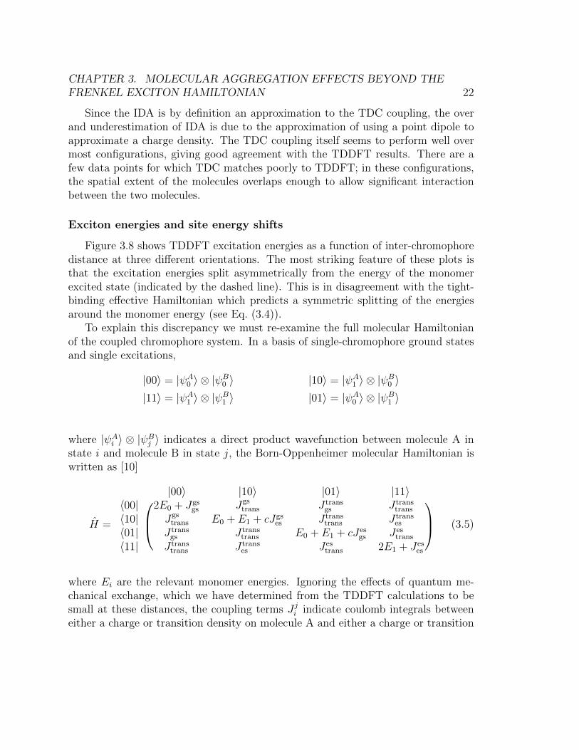
Since the IDA is by definition an approximation to the TDC coupling, the overand underestimation of IDA is due to the approximation of using a point dipole toapproximate a charge density. The TDC coupling itself seems to perform well overmost configurations, giving good agreement with the TDDFT results. There are afew data points for which TDC matches poorly to TDDFT; in these configurations,the spatial extent of the molecules overlaps enough to allow significant interactionbetween the two molecules.
Exciton energies and site energy shifts
Figure 3.8 shows TDDFT excitation energies as a function of inter-chromophoredistance at three different orientations. The most striking feature of these plots isthat the excitation energies split asymmetrically from the energy of the monomerexcited state (indicated by the dashed line). This is in disagreement with the tight-binding effective Hamiltonian which predicts a symmetric splitting of the energiesaround the monomer energy (see Eq. (3.4)).
To explain this discrepancy we must re-examine the full molecular Hamiltonianof the coupled chromophore system. In a basis of single-chromophore ground statesand single excitations,
|00〉 = |ψA0 〉 ⊗ |ψB0 〉 |10〉 = |ψA1 〉 ⊗ |ψB0 〉|11〉 = |ψA1 〉 ⊗ |ψB1 〉 |01〉 = |ψA0 〉 ⊗ |ψB1 〉
where |ψAi 〉 ⊗ |ψBj 〉 indicates a direct product wavefunction between molecule A instate i and molecule B in state j, the Born-Oppenheimer molecular Hamiltonian iswritten as [10]
H =
|00〉 |10〉 |01〉 |11〉
〈00| 2E0 + Jgsgs Jgs
trans J transgs J trans
trans
〈10| Jgstrans E0 + E1 + cJgs
es J transtrans J trans
es
〈01| J transgs J trans
trans E0 + E1 + cJesgs Jes
trans
〈11| J transtrans J trans
es Jestrans 2E1 + Jes
es
(3.5)
where Ei are the relevant monomer energies. Ignoring the effects of quantum me-chanical exchange, which we have determined from the TDDFT calculations to besmall at these distances, the coupling terms J ji indicate coulomb integrals betweeneither a charge or transition density on molecule A and either a charge or transition
CHAPTER 3. MOLECULAR AGGREGATION EFFECTS BEYOND THEFRENKEL EXCITON HAMILTONIAN 23
Parallel-0◦
30°
Parallel-30◦
Anti-Parallel-0◦
Figure 3.7: The energy splittings between the dimer excited states are shown for TDDFT,
TDC and IDA calculations. The TDDFT points show E2−E12 , while the TDC and IDA
lines show ε+−ε−2 with the J coupling calculated using the respective approximation. The
TDC and TDDFT predictions mostly overlap.
CHAPTER 3. MOLECULAR AGGREGATION EFFECTS BEYOND THEFRENKEL EXCITON HAMILTONIAN 24
Parallel-0◦
30°
Parallel-30◦
Anti-Parallel-0◦
Figure 3.8: TDDFT excitation energies (E1 − E0 and E2 − E0) for the coupled excitedstates of the coumarin-343-MA dimer. Orientation of the dimer is shown to the right.Erroneous charge transfer states are not shown, since they do not mix into the opticalstates (explained in Figure 3.12).
CHAPTER 3. MOLECULAR AGGREGATION EFFECTS BEYOND THEFRENKEL EXCITON HAMILTONIAN 25
density on molecule B, i.e.
J ji =
∫ρAi (r1)
1
|r1 − r2|ρBj (r2)dr1dr2. (3.6)
with i, j equal to either gs (ground state charge density), es (excited state chargedensity), or trans (transition density). The charge densities and transition densitiesare defined for molecule A as
ρAgs(r1) = N
∫· · ·∫ψA∗0 (r1, r2 . . . rN)ψA0 (r1, r2 . . . rN)dr2 . . . drN ×
∑n∈A
Znδ(Rn − r1) (3.7)
ρAes(r1) = N
∫· · ·∫ψB∗1 (r1, r2 . . . rN)ψB1 (r1, r2 . . . rN)dr2 . . . drN ×
∑n∈B
Znδ(Rn − r1) (3.8)
ρAtrans(r1) =
∫· · ·∫ψA∗0 (r1, r2 . . . rN)ψA1 (r1, r2 . . . rN)dr2 . . . drN , (3.9)
and similarly for molecule B, where Zn and Rn correspond to the charge and positionsof the nuclei in their respective molecules, and N is the total number of electronsin a molecule. The coefficient c is a parameter used to scale the magnitude of theground-state/excited-state Coulomb integral (see discussion below).
In order to reduce this Hamiltonian into the tight-binding effective Hamiltonian inEq. (3.3) a number of approximations must be made. Firstly, the Coulomb integralsare assumed to be much smaller than the energetic differences and therefore thematrix in Eq. (3.5) is approximated as block diagonal, with each block labeled bythe number of excited states. Explicitly, J ji � E1 −E0 but Jgs
es ≈ Jesgs , and therefore
we can ignore all off-diagonal terms except for those coupling |10〉 and |01〉. Thisapproximation is sometimes referred to as the Heitler-London approximation in theliterature [68]. Typically, the intermolecular Coulomb interaction terms are ignoredi.e., one assumes that Jgs
gs ≈ Jgses ≈ Jes
gs ≈ 0, and then the only Coulomb interactionterms that remain are the J trans
trans terms. Under this approximation the in the singleexcitation subspace (after a shift of the diagonal energies by 2E0) is the one given inEq. (3.3),
H − 2E0 =
|10〉 |01〉( )〈10| ε0 J trans
trans
〈01| J transtrans ε0
(3.10)
with ε0 = E1 − E0.We assess the validity of these approximations by evaluating the expanded 4× 4
effective Eq. (3.5). In order to calculate the matrix elements of this larger we use
CHAPTER 3. MOLECULAR AGGREGATION EFFECTS BEYOND THEFRENKEL EXCITON HAMILTONIAN 26
Mulliken partial atomic charges [69] for the ground state and excited state densi-ties instead of density cubes. This is because density cube calculations are not con-strained to reproduce the correct multipole expansion of the electron densities. Theseerrors can be corrected for the transition density, as shown by Kreuger et al. [30],however the errors are more pronounced in the ground state and excited state densi-ties, making them sensitive to the choice of grid resolution. In Figure 3.10, we showthe results of using this expanded effective . It is evident from Figure 3.10 that weare able to reproduce the asymmetric shifts in excitonic energies using Eq. (3.5).
The primary effects that invalidate the approximations leading to Eq. (3.10) areelectrostatic in nature. The neglect of the Jes
trans, Jgstrans, J
transes , J trans
es and the J transtrans
terms coupling the ground state |00〉 to the two-exciton state |11〉 (Heitler-Londonapproximation) is valid since these are much less than E1 − E0 at all the inter-chromophore distance scales we examined. However, the electrostatic corrections tothe diagonal elements of Eq. (3.5), Jgs
gs , Jgses , J
esgs , J
eses , are significant and cannot be
neglected. These are shifts to monomer energies due to the presence of the chargeson the other chromophore. These electrostatic shifts are dependent on the inter-chromophoric distance and the exact orientation of the chromophores. Using theMulliken partial atomic charge approach we are able to capture these electrostaticshifts and thereby get very good agreement with the TDDFT energies. The staticdipole for the ground state and excited state both lie nearly parallel to the transitiondipole moment. Consequently, the direction of the shifts is consistent with what isexpected from the interaction of two electronic dipoles - the parallel dimers have arepulsive electrostatic effect while the anti-parallel dimers have an attractive effect.
While the asymmetric splitting is immediately captured by including these elec-trostatic distance-dependent shifts, scaling the ground-state/excited-state coulombintegrals by c = 0.66 is necessary in order to achieve quantitative agreement with theTDDFT energies. The value of this scaling factor is specific to a chromophore pair,but once determined for a particular orientation and distance separation, it holds fornearly all inter-chromophore separations and orientations. We have confirmed thisby explicit calculation of energies at additional orientations and distances not pre-sented in Figure 3.10. We interpret this parameter as the screening of the Coulombintegral by the other electrons in the molecular dimer.
We remark here that similar electrostatic shifts of proximal chromophores wereidentified in Ref. [70]. Such electrostatic shifts to monomer energies can be a signifi-cant source of disorder in multi-chromophoric assemblies. It is widely accepted thatprotein residues cause energetic shifts that are important for providing a favorableenergetic landscape for energy transfer [71]. Our results indicate that in additionto the effect of the proteins, the electrostatic environment provided by neighboringchromophores should also be taken into account when calculating energetic shifts
CHAPTER 3. MOLECULAR AGGREGATION EFFECTS BEYOND THEFRENKEL EXCITON HAMILTONIAN 27
and disorder in multi-chromophoric arrays. From a design perspective, this impliesthat the exact orientation and placement of chromophores are important not onlyfor the precise engineering of the excitonic coupling between chromophores but alsofor engineering the energetic landscape.
6 8 10 12 14 16 18
Distance [ ]
3.42
3.44
3.46
3.48
3.50
3.52
3.54
3.56
Exc
itatio
n E
nerg
y [e
V]
monomer transition energyvacuumcyclohexanemethanolwater
Figure 3.9: TDDFT excitation energies (E1 − E0 and E2 − E0) for the coupled ex-cited states of the coumarin-343-MA dimer in various solvent environments (modeled usingPCM). Only results for the parallel oriented dimer are shown.
We note that the electrostatic shifts identified here can be strongly affected bythe polarity of the solvent [36]. In particular, charge screening by a polar solvent canreduce the value of electrostatic integrals such as Jes
gs . These integrals are likely to bemore suppressed than the transition density integrals, e.g. J trans
trans , and therefore theenergy shifts can be suppressed even though the excitonic coupling (which is largelydetermined by J trans
trans ) may be only marginally effected by solvent screening [37].To demonstrate this we calculated the excitations energies of the coumarin-343-MAhomo-dimer in various solvent environments modeled using a polarizable continuummodel (PCM). The results are shown in Figure 3.9 for the parallel oriented dimer.Clearly, as the polarity of the solvent increases the asymmetry of the excitationenergy splitting around the monomer energy decreases. This demonstrates that itis important to integrate information about the solvent environment when modelingexcitonic properties of molecular aggregates; solvent polarity will dictate the amountof influence electrostatic effects have on excitonic energies.
CHAPTER 3. MOLECULAR AGGREGATION EFFECTS BEYOND THEFRENKEL EXCITON HAMILTONIAN 28
6 8 10 12 14 16 18
Distance [ ]
3.42
3.44
3.46
3.48
3.50
3.52
3.54
3.56
3.58
3.60
Exc
itatio
n E
nerg
y [e
V]
monomer transition energyTDDFT bright stateTDDFT dark stateλ2−λ0
λ1−λ0
λ2−λ0 scaledλ1−λ0 scaled
Parallel-0◦
6 8 10 12 14 16 18
Distance [ ]
3.30
3.32
3.34
3.36
3.38
3.40
3.42
3.44
3.46
Exc
itatio
n E
nerg
y [e
V]
monomer transition energyTDDFT bright stateTDDFT dark stateλ2−λ0
λ1−λ0
λ2−λ0 scaledλ1−λ0 scaled
Anti-Parallel-0◦
Figure 3.10: The energy levels calculated using TDDFT are together with the excitedstates of the 4x4 in Eq. (3.5). For the latter, the excited states are plotted as λ1 − λ0 andλ2 − λ0 where λi is the ith eigenvalue.
CHAPTER 3. MOLECULAR AGGREGATION EFFECTS BEYOND THEFRENKEL EXCITON HAMILTONIAN 29
Exciton wave functions
We now investigate the character of the TDDFT excited states to examine whetherthey are well described by products of monomer wavefunctions, as predicted byEq. (3.4). The tight-binding effective description of the excited states can breakdown if either the dimer orbitals change with respect to the monomer orbitals, orthe nature of the excited state changes significantly as a function of distance. TheTDDFT excited states are written as linear combinations of basis functions whichrepresent single-particle excitations from the DFT ground state. If the coefficientsof this linear expansion are distance-dependent, the predictions of the effective inEq. (3.3) are invalid. This is because the exciton wave functions in Eq. (3.4) are con-structed from symmetric and anti-symmetric combinations of the monomer states(i.e. Eq. (3.4)), and are therefore independent of the magnitude of the coupling en-ergy J and hence of the inter-chromophoric separation. Figure 3.11 shows thesecoefficients for the bright state of the parallel orientation of the monomers as a func-tion of distance. We see from this figure that the nature of the TDDFT excited stateis relatively constant as a function of distance, until we get to small separation dis-tances (below 8 A). In particular, the dominant single-particle excitation, that fromthe highest occupied molecular orbital (HOMO) to the lowest unoccupied molecularorbital (LUMO) on each monomer, begins to change at intermolecular distances lessthan 8 A. However, some of the other minor excitations which contribute to theTDDFT excited state begin to change gradually as a function of distance already at12 A.
Some of the single-particle excitations which contribute below 7 A representcharge-transfer excitations from molecule A to molecule B. The existence of chargetransfer, especially between 6 and 7 A, is a feature present also for range-correctedTDDFT functionals (Figure 3.12). It is well known that TD-B3LYP is poor atpredicting the energetics of charge transfer states, as are other functionals without100% Hartree-Fock exchange [72, 73]. Figure 3.12 shows that TD-B3LYP predictslow-lying charge transfer states for the coumarin-343-MA dimer. However, the range-corrected DFT calculations show that the charge transfer states are much higher inenergy. The splitting between the exciton states is consistent between B3LYP andthe range corrected calculations. This suggests that the low lying charge transferstates predicted by B3LYP do not affect the character of the exciton states. There-fore, we may safely disregard these charge transfer states and use only the excitonstates in our analysis.
In Figure 3.13, we show the overlap integral of the monomer molecular orbitals
CHAPTER 3. MOLECULAR AGGREGATION EFFECTS BEYOND THEFRENKEL EXCITON HAMILTONIAN 30
0.0 0.2 0.4 0.6 0.8 1.00.0
0.2
0.4
0.6
0.8
1.0
ψLAHA
ψLBHB
ψL+1AH−3A
ψL+1BH−3B
ψL+2AHA
ψL+2BHB
ψL+2AH−3A
ψL+2BH−3B
ψL+2AH−4A
ψL+2BH−4B
ψLBHA
ψLAHB
ψL+1BH−3A
ψL+1AH−3B
ψL+2BHA
ψL+2AHB
0.0 0.2 0.4 0.6 0.8 1.0
Distance [ ]
0.0
0.2
0.4
0.6
0.8
1.0
Exc
itatio
n A
mpl
itude
0.65
0.70
0.75
6 8 10 12 14 16 180.00
0.05
0.10
Figure 3.11: The expansion coefficients of the parallel-oriented bright state shown as afunction of distance. Dashed lines represent the corresponding coefficients in the monomerTDDFT excited states. The top panel shows the dominant single-particle excitation, whichcorresponds to the excitation of an electron in the highest occupied molecular orbital(HOMO) to the lowest unoccupied molecular orbital (LUMO) of each monomer. Thebottom panel shows other single-particle excitations which make up the TDDFT excitedstate. Molecular orbitals are labeled with respect to their energetic position below theHOMO (H − n) or above the LUMO (L+ n). The excitations that are doubly degenerate(e.g. ψLA
HAand ψLB
HB) have been averaged and plotted without their molecule index.
and the corresponding dimer orbitals,∫φdimern (r)φmonomer
n (r)dr. (3.11)
In the limit of infinite separation between the two dyes, each dimer molecular orbitalis doubly degenerate, possessing unit overlap with a corresponding monomer molec-ular orbital. For the HOMO and LUMO, which are the most important orbitals inthe bright state (Figure 3.11), the correspondence between monomer and dimer MOsis almost perfect for distances greater than 7 A. Between 6 and 7 A, these orbitalschange by about 8% . Some orbitals change already at larger distances, such as theLUMO+1 and the LUMO+2 orbitals, which begin to deform as the intermoleculardistance is decreased below 8 A. Finally, the HOMO-3, which with the LUMO+1forms the next most dominant excitation in the bright state, changes continuously
CHAPTER 3. MOLECULAR AGGREGATION EFFECTS BEYOND THEFRENKEL EXCITON HAMILTONIAN 31
6.0 6.5 7.0 7.5 8.0 8.5 9.0 9.5 10.0
Distance [◦A]
3.2
3.4
3.6
3.8
4.0
4.2
4.4E
xcita
tion
Ene
rgy
[eV
]
B3LYPBLYP: µ=2.0−1
BLYP: µ=2.5−1
BLYP: µ=3.0−1
BLYP: µ=3.5−1
BLYP: µ=4.0−1
Figure 3.12: Coumarin-343 energy levels predicted by B3LYP and range-corrected BLYP.The coupled exciton states (solid lines) for B3LYP and the range corrected calculationsare shown overlapped, while the energies of the charge transfer states (dashed lines) variesbased on the functional. The range corrected BLYP energies have been shifted such thatthe first excited state energies of the monomer calculations are all aligned to that of B3LYP.This is done to compare the energies of the charge transfer states relative to the coupledexciton states.
at distances less than 18 A; however, it changes by only 2% and furthermore it doesnot form the majority of the excited state, so this effect is diminished in the excitedstate energies and couplings.
To summarize this investigation of excited state wave functions, we find that forcoumarin-343-MA, it is reasonable to describe the dimer wavefunctions in a basisof monomer wavefunctions for separation distances greater than 8 A. For smallerdistances the B3LYP calculations indicate possible mixing in of charge transfer char-acter into the excited state wavefunction, although the extent of this mixing is notconclusive from this level of calculation.
3.4 Conclusions
In this work we have made a critical assessment of the conventional effectiveapproach of modeling the excitonic properties of molecular aggregates, using the
CHAPTER 3. MOLECULAR AGGREGATION EFFECTS BEYOND THEFRENKEL EXCITON HAMILTONIAN 32
6 8 10 12 14 16 18
Distance [◦A]
0.80
0.85
0.90
0.95
1.00O
verla
p In
tegr
al
HOMO-4HOMO-3HOMOLUMOLUMO+1LUMO+2
Figure 3.13: Overlaps of the bright state dimer molecular orbitals with their correspondingmonomer molecular orbitals (See Eq. (3.11))
coumarin-343-MA dye as a case study. Results from ab-initio electronic structurecalculations using TDDFT were compared with predictions from the conventionaltight-binding effective for a homo-dimer (the Heitler-London approximation). Mostinterestingly, we found that the conventional effective for a homo-dimer does notreproduce the asymmetric energy splittings calculated using TDDFT. In particular,the ideal dipole approximation of the excited state coupling was found to give a veryinaccurate representation of the TDDFT energy splittings. While the TDC methodwas found to perform much better, both the IDA and the TDC descriptions werefound to be unable to reproduce the asymmetric nature of the splitting betweenbright and dark state energy levels that is predicted from TDDFT. We showed thatthis is a result of ignoring non-negligible electrostatic energy shifts resulting fromthe proximity of the two chromophores. We outlined a method for reincorporat-ing these electrostatic shifts using a simple approach that only requires calculatingCoulomb integrals based on Mulliken partial atomic charges. This approach is anefficient method for forming more complete effective descriptions that capture allthe relevant physical effects; it only requires TDDFT calculations of dimers of chro-mophores (of each dimer combination of species present in the aggregate) and theremaining elements are accurately captured by Coulomb integrals. We find that thecombination of a TDC description of the transition density coupling together withproper incorporation of electrostatic shifts produces an excellent effective descrip-tion of excitonics in molecular aggregates. We also demonstrated the importance of
CHAPTER 3. MOLECULAR AGGREGATION EFFECTS BEYOND THEFRENKEL EXCITON HAMILTONIAN 33
incorporating details of solvent polarity into the molecular aggregate model, sincethis also determines the degree of influence the electrostatic effects have on excitonicenergies.
Additionally, we scrutinized the assumptions of the conventional Heitler-Londontight-binding picture of excitonic coupling, by examining changes in the character ofthe excited state and the coupled molecular orbitals as a function of intermoleculardistance. These effects were determined to be small but nonzero for intermoleculardistances greater than 7-8 A, while TDDFT predicts a significant departure from theHeitler-London picture at smaller distances. It also predicts some charge-transfercharacter at these smaller distances. In the future it would be useful to developmore reliable estimates of this charge-transfer character [15] in order to analyze theinterplay between excitonic and charge transfer states in chromophore arrays relevantto natural photosynthesis, such as, e.g., the bacterial reaction center [74].
We expect that our investigation and refinement of effective Hamiltonian descrip-tions of molecular aggregates will inform the modeling of large molecular aggregatesformed by direct aggregation or aggregation by protein templated assembly. Suchaggregates show promise as the basis for next-generation light harvesting or sensingdevices with tailored properties, and efficient modeling of their excitonic propertiesthrough effective Hamiltonians will be important for rational design and engineeringof such devices.
34
Chapter 4
Unified description of excitationenergy transfer and chargeseparation
4.1 Introduction
Organic photovoltaic (OPV) cells can be low-cost, light-weight, and flexible, mak-ing them a promising alternative to silicon based photovoltaic cells.[75, 76] The powerconversion efficiencies of the best OPV cells has recently exceeded 10% [77, 78], yetthis is still far from the theoretical limit of efficiency (20-24%) for single-junction OPVcells.[79] Typical organic semiconductors have low dielectric constants,[80] usually inthe range 2–5 vs. 11.7 for bulk monocrystalline silicon.[81] Consequently, electrostaticinteractions between charges in organic materials are not effectively screened, and in-teraction with light predominantly produces excitons (Coulomb-bound electron-holepairs), rather than free charge carriers.[82] To generate a current in an OPV cell,the electron and the hole that form an exciton must move in opposite directions.However, the exciton binding energy often exceeds the available thermal energy byan order of magnitude or more.[83] The energy needed for spatially separating theelectron and the hole is therefore typically supplied by the local electric field at aninterface between a domain of electron-donating and electron-accepting molecules(D-A interface).
One factor limiting the efficiency of OPV cells is the bimolecular recombination ofexcitons before they reach a D-A interface.[84] To minimize recombination, typicalOPV cells rely on bulk heterojunctions: purposely disordered blends of electron-donor and electron-acceptor materials with linear dimensions of donor and acceptor
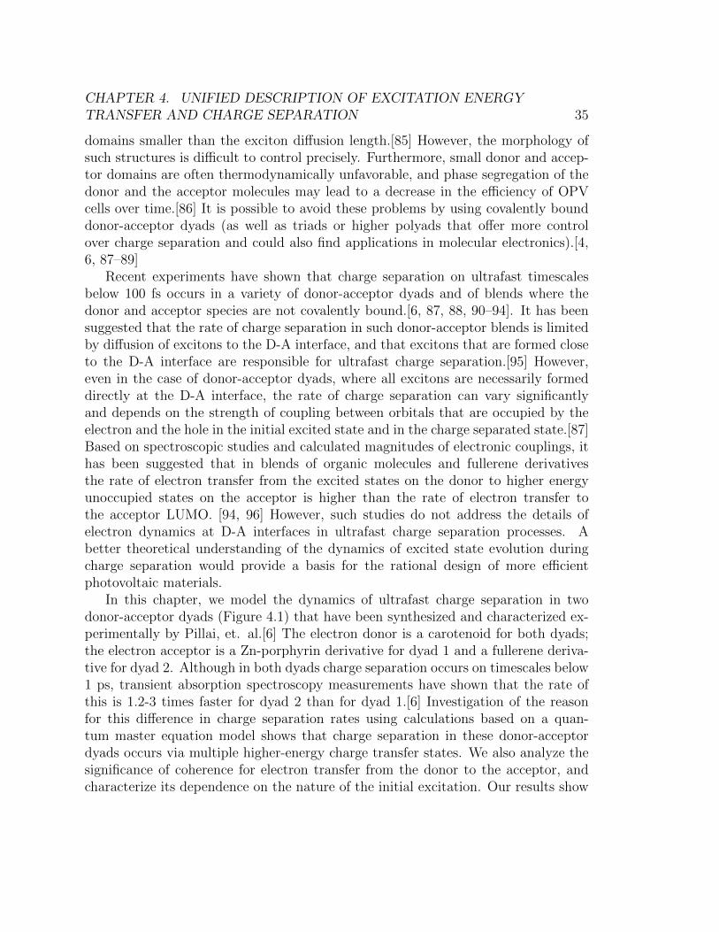
CHAPTER 4. UNIFIED DESCRIPTION OF EXCITATION ENERGYTRANSFER AND CHARGE SEPARATION 35
domains smaller than the exciton diffusion length.[85] However, the morphology ofsuch structures is difficult to control precisely. Furthermore, small donor and accep-tor domains are often thermodynamically unfavorable, and phase segregation of thedonor and the acceptor molecules may lead to a decrease in the efficiency of OPVcells over time.[86] It is possible to avoid these problems by using covalently bounddonor-acceptor dyads (as well as triads or higher polyads that offer more controlover charge separation and could also find applications in molecular electronics).[4,6, 87–89]
Recent experiments have shown that charge separation on ultrafast timescalesbelow 100 fs occurs in a variety of donor-acceptor dyads and of blends where thedonor and acceptor species are not covalently bound.[6, 87, 88, 90–94]. It has beensuggested that the rate of charge separation in such donor-acceptor blends is limitedby diffusion of excitons to the D-A interface, and that excitons that are formed closeto the D-A interface are responsible for ultrafast charge separation.[95] However,even in the case of donor-acceptor dyads, where all excitons are necessarily formeddirectly at the D-A interface, the rate of charge separation can vary significantlyand depends on the strength of coupling between orbitals that are occupied by theelectron and the hole in the initial excited state and in the charge separated state.[87]Based on spectroscopic studies and calculated magnitudes of electronic couplings, ithas been suggested that in blends of organic molecules and fullerene derivativesthe rate of electron transfer from the excited states on the donor to higher energyunoccupied states on the acceptor is higher than the rate of electron transfer tothe acceptor LUMO. [94, 96] However, such studies do not address the details ofelectron dynamics at D-A interfaces in ultrafast charge separation processes. Abetter theoretical understanding of the dynamics of excited state evolution duringcharge separation would provide a basis for the rational design of more efficientphotovoltaic materials.
In this chapter, we model the dynamics of ultrafast charge separation in twodonor-acceptor dyads (Figure 4.1) that have been synthesized and characterized ex-perimentally by Pillai, et. al.[6] The electron donor is a carotenoid for both dyads;the electron acceptor is a Zn-porphyrin derivative for dyad 1 and a fullerene deriva-tive for dyad 2. Although in both dyads charge separation occurs on timescales below1 ps, transient absorption spectroscopy measurements have shown that the rate ofthis is 1.2-3 times faster for dyad 2 than for dyad 1.[6] Investigation of the reasonfor this difference in charge separation rates using calculations based on a quan-tum master equation model shows that charge separation in these donor-acceptordyads occurs via multiple higher-energy charge transfer states. We also analyze thesignificance of coherence for electron transfer from the donor to the acceptor, andcharacterize its dependence on the nature of the initial excitation. Our results show
CHAPTER 4. UNIFIED DESCRIPTION OF EXCITATION ENERGYTRANSFER AND CHARGE SEPARATION 36
HN
O
N
NN
NZn
CNNC
CNCN
(a) Dyad 1
NPF6
(b) Dyad 2
Figure 4.1: Molecular structures of dyads 1 and 2. The donor fragment (shown in blue)is a carotenoid for both dyads, and the acceptor fragment (red) is a porphyrin for dyad 1and fullerene for dyad 2.
that higher energy acceptor states must be included in simulations in order to ob-tain accurate charge separation rates and reveal key design principles for optimizingultrafast charge separation.
4.2 Methods
We simulated charge transfer in two molecular dyads (Figure 4.1) that have beensynthesized and spectroscopically studied by Pillai et al.[6] The geometries of bothdyads were optimized using the Q-Chem electronic structure package’s implementa-tion of density functional theory (DFT), with the B3LYP hybrid exchange-correlationfunctional and the 6-31G* basis set.[97] Each dyad was partitioned into a donorand an acceptor fragment. The donor fragment (shown in blue in Figure 4.1) is acarotenoid for both dyads, and the acceptor fragment (shown in red in Figure 4.1) isa porphyrin derivative for dyad 1 and a fullerene derivative for dyad 2. The boundarybetween the donor and acceptor fragments was chosen so that the donor fragmenthas similar electronic properties in both dyads.
Transient absorption spectroscopy has been used to track the electron and ex-citon dynamics in both dyads after an initial excitation to the (bright) second ex-cited state of the carotenoid (donor).[6] For carotenoids, the lowest energy excitedstate is typically a (dark) double excitation state that is not captured by standardtime-dependent density functional theory (TDDFT) calculations[98]. Experimentalresults suggest that the initial excitation can undergo efficient internal conversion,on a timescale of the order of 100 fs, to the lowest-energy carotenoid excited state.
CHAPTER 4. UNIFIED DESCRIPTION OF EXCITATION ENERGYTRANSFER AND CHARGE SEPARATION 37
However, charge separation from this state has a timescale of about 11 ps for dyad1 and is also on the order of several picoseconds for dyad 2.[6] This state acts asa trap state and decreases the yield of subpicosecond charge separation that is thefocus of our study, but does not significantly affect its dynamics. Therefore, we donot include this state in the simulations presented in this chapter.
The carotenoid’s orbitals are well separated in energy, therefore higher excitedstates on the donor fragment are not significantly populated during the charge sep-aration process. Only the lowest two single-excitation states on the carotenoid con-tribute to ultrafast charge separation and thus need to be included in the simulations.
For dyad 1, transient absorption spectroscopy suggests that exciton transfer fromthe donor to the acceptor fragment is negligible.[6] This is likely due to the lowtransition dipole strength of the Q-band in porphyrins, which is an order of magni-tude smaller than in structurally similar materials that are known for efficient energytransfer, such as chlorophylls, pyropheophorbides, and phthalocyanines.[99] There-fore, excitons localized on the acceptor need not be included in simulations of chargeseparation in dyad 1.
For dyad 2, the rate of resonant energy transfer between the donor and theacceptor fragments is comparable to the rate of valence electron transfer, but the rateof hole transfer from the acceptor to the donor is an order of magnitude smaller.[6]Consequently, excitons localized on the acceptor have a negligible direct contributionto charge separation in dyad 2: rather, they can undergo efficient energy transfer backto the donor, followed by efficient electron transfer to the acceptor. Because energytransfer between the acceptor and the donor is not a rate-limiting step, excitonslocalized on the acceptor have little effect on the rate of charge separation. Therefore,these states do not need to be included in simulations of charge separation in dyad2.
The two Frenkel exciton states on the carotenoid that are populated within thefirst 100 fs of excitation can transfer the excited electron to a number of unoccu-pied acceptor orbitals. In our simulations, we include as many lowest-energy chargetransfer (CT) states with the hole on the donor and the electron on the acceptor asare necessary for convergence of the charge separation rates: 20 CT states for dyad1 and 28 CT states for dyad 2. The complete basis set for our charge separationsimulations consists then of two Frenkel excitons localized on the donor fragment,and charge transfer states with the electron on the acceptor and the hole on thedonor. We will henceforth refer to the Frenkel exciton states with the electron inthe donor LUMO or LUMO+1 as Exc1 and Exc2, respectively, and to the chargetransfer states, enumerated by increasing energy, as CT3, CT4, ..., CTN (N = 22 fordyad 1 and N = 30 for dyad 2).
CHAPTER 4. UNIFIED DESCRIPTION OF EXCITATION ENERGYTRANSFER AND CHARGE SEPARATION 38
Using this basis set, we construct a tight binding Hamiltonian for the dyad:
H =N∑i=1
εia†i ai +
N∑i=1
i−1∑j=1
Jij
(a†i aj + aia
†j
), (4.1)
where a†i and ai are creation and annihilation operators, respectively, for basis statei, εi is the energy of state i, and Jij is the coupling between states i and j.
For excitonic states, Exci (i = 1, 2), εi are given by the TDDFT excitationenergies that correspond to the HOMO-LUMO and HOMO-LUMO+1 excitations,respectively. These energies account for the difference in orbital energies, as well asthe binding energy of the exciton.
The energies of charge transfer states, CTi (i = 3, N), are given by:
εi = EAi − ED − e2
4πε0
∫dr1dr2
∣∣φAi (r1)
∣∣2 ∣∣φD (r2)∣∣2
|r1 − r2|, (4.2)
where φD(r) and ED are the HOMO of the donor fragment and its energy, φAi (r)
and EAi are the ith unoccupied orbital of the acceptor fragment and its energy, ε0 is
the vacuum permittivity, and the integration is over all space. This expression ap-proximates the donor cation and acceptor anion energies using Koopman’s theorem,and the binding energy as the Coulomb attraction between the electron and holeprobability densities.
The fragment molecular orbital energies and probability densities in Eq. (4.2) areobtained from Kohn-Sham density functional theory using the Amsterdam DensityFunctional package (ADF) [100] with the B3LYP hybrid exchange-correlation func-tional using a double-zeta polarized basis set, DZP. In order to obtain the couplingsJij, the fragment orbitals can be used as a basis set in a subsequent DFT calcula-tion on the entire dyad.[101–103] In this basis, the coupling between two fragmentorbitals is the generalized charge transfer integral[104]:
Jij =HKSij − 1
2Sij(HKSii +HKS
jj
)1− S2
ij
, (4.3)
where HKS is the dyad Kohn-Sham Hamiltonian and S is the overlap matrix.Although perturbative Markovian master equations are known to underestimate
coherence lifetimes for charge and energy transfer processes [105], they neverthelessdo describe the overall rate of population transfer rather well [106]. Therefore, asin an earlier paper that examines exciton and charge transfer dynamics in systemsconsisting of multiple interacting chromophores,[107] we describe the dynamics of
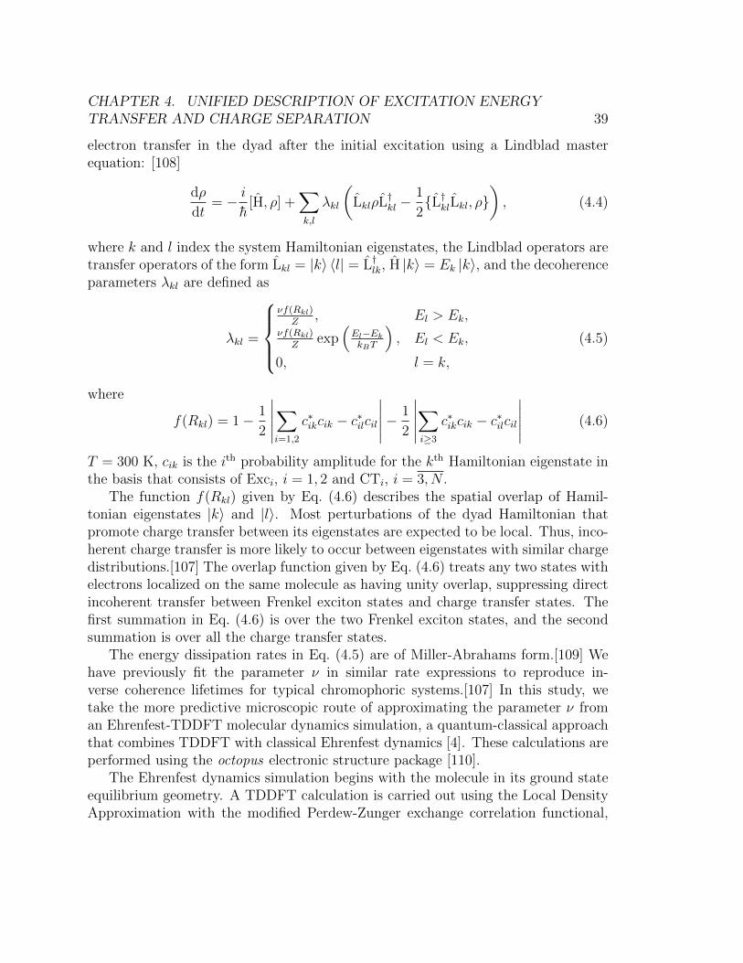
CHAPTER 4. UNIFIED DESCRIPTION OF EXCITATION ENERGYTRANSFER AND CHARGE SEPARATION 39
electron transfer in the dyad after the initial excitation using a Lindblad masterequation: [108]
dρ
dt= − i
h[H, ρ] +
∑k,l
λkl
(LklρL†kl −
1
2{L†klLkl, ρ}
), (4.4)
where k and l index the system Hamiltonian eigenstates, the Lindblad operators aretransfer operators of the form Lkl = |k〉 〈l| = L†lk, H |k〉 = Ek |k〉, and the decoherenceparameters λkl are defined as
λkl =
νf(Rkl)
Z, El > Ek,
νf(Rkl)Z
exp(El−Ek
kBT
), El < Ek,
0, l = k,
(4.5)
where
f(Rkl) = 1− 1
2
∣∣∣∣∣∑i=1,2
c∗ikcik − c∗ilcil
∣∣∣∣∣− 1
2
∣∣∣∣∣∑i≥3
c∗ikcik − c∗ilcil
∣∣∣∣∣ (4.6)
T = 300 K, cik is the ith probability amplitude for the kth Hamiltonian eigenstate inthe basis that consists of Exci, i = 1, 2 and CTi, i = 3, N .
The function f(Rkl) given by Eq. (4.6) describes the spatial overlap of Hamil-tonian eigenstates |k〉 and |l〉. Most perturbations of the dyad Hamiltonian thatpromote charge transfer between its eigenstates are expected to be local. Thus, inco-herent charge transfer is more likely to occur between eigenstates with similar chargedistributions.[107] The overlap function given by Eq. (4.6) treats any two states withelectrons localized on the same molecule as having unity overlap, suppressing directincoherent transfer between Frenkel exciton states and charge transfer states. Thefirst summation in Eq. (4.6) is over the two Frenkel exciton states, and the secondsummation is over all the charge transfer states.
The energy dissipation rates in Eq. (4.5) are of Miller-Abrahams form.[109] Wehave previously fit the parameter ν in similar rate expressions to reproduce in-verse coherence lifetimes for typical chromophoric systems.[107] In this study, wetake the more predictive microscopic route of approximating the parameter ν froman Ehrenfest-TDDFT molecular dynamics simulation, a quantum-classical approachthat combines TDDFT with classical Ehrenfest dynamics [4]. These calculations areperformed using the octopus electronic structure package [110].
The Ehrenfest dynamics simulation begins with the molecule in its ground stateequilibrium geometry. A TDDFT calculation is carried out using the Local DensityApproximation with the modified Perdew-Zunger exchange correlation functional,
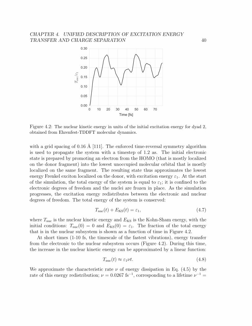
CHAPTER 4. UNIFIED DESCRIPTION OF EXCITATION ENERGYTRANSFER AND CHARGE SEPARATION 40
0 10 20 30 40 50 60 70Time [fs]
0.00
0.05
0.10
0.15
0.20
0.25
0.30
Tnuc/ε
1
Figure 4.2: The nuclear kinetic energy in units of the initial excitation energy for dyad 2,obtained from Ehrenfest-TDDFT molecular dynamics.
with a grid spacing of 0.16 A [111]. The enforced time-reversal symmetry algorithmis used to propagate the system with a timestep of 1.2 as. The initial electronicstate is prepared by promoting an electron from the HOMO (that is mostly localizedon the donor fragment) into the lowest unoccupied molecular orbital that is mostlylocalized on the same fragment. The resulting state thus approximates the lowestenergy Frenkel exciton localized on the donor, with excitation energy ε1. At the startof the simulation, the total energy of the system is equal to ε1; it is confined to theelectronic degrees of freedom and the nuclei are frozen in place. As the simulationprogresses, the excitation energy redistributes between the electronic and nucleardegrees of freedom. The total energy of the system is conserved:
Tnuc(t) + EKS(t) = ε1, (4.7)
where Tnuc is the nuclear kinetic energy and EKS is the Kohn-Sham energy, with theinitial conditions: Tnuc(0) = 0 and EKS(0) = ε1. The fraction of the total energythat is in the nuclear subsystem is shown as a function of time in Figure 4.2.
At short times (1-10 fs, the timescale of the fastest vibrations), energy transferfrom the electronic to the nuclear subsystem occurs (Figure 4.2). During this time,the increase in the nuclear kinetic energy can be approximated by a linear function:
Tnuc(t) ≈ ε1νt. (4.8)
We approximate the characteristic rate ν of energy dissipation in Eq. (4.5) by therate of this energy redistribution; ν = 0.0267 fs−1, corresponding to a lifetime ν−1 =
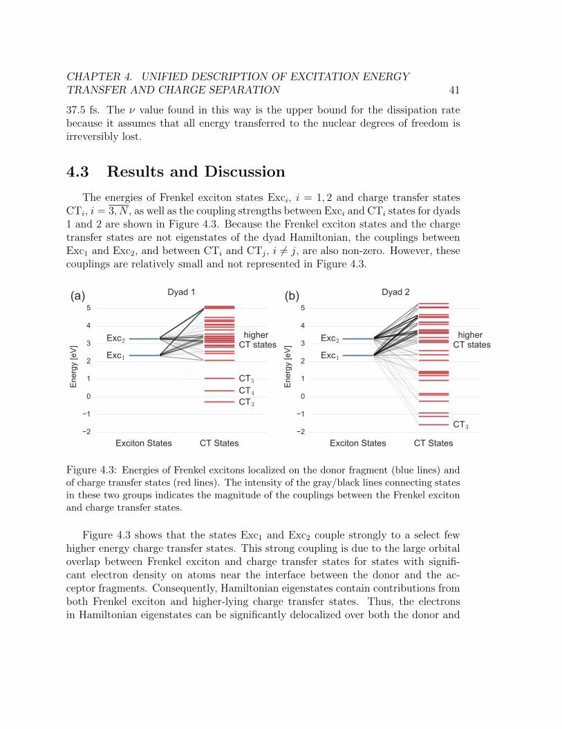
CHAPTER 4. UNIFIED DESCRIPTION OF EXCITATION ENERGYTRANSFER AND CHARGE SEPARATION 41
37.5 fs. The ν value found in this way is the upper bound for the dissipation ratebecause it assumes that all energy transferred to the nuclear degrees of freedom isirreversibly lost.
4.3 Results and Discussion
The energies of Frenkel exciton states Exci, i = 1, 2 and charge transfer statesCTi, i = 3, N , as well as the coupling strengths between Exci and CTi states for dyads1 and 2 are shown in Figure 4.3. Because the Frenkel exciton states and the chargetransfer states are not eigenstates of the dyad Hamiltonian, the couplings betweenExc1 and Exc2, and between CTi and CTj, i 6= j, are also non-zero. However, thesecouplings are relatively small and not represented in Figure 4.3.
2
1
0
1
2
3
4
5
Ener
gy [e
V]
Exciton States CT States
Exc1
Exc2
CT3
CT4
CT5
higher CT states
(a) Dyad 1
2
1
0
1
2
3
4
5
Ener
gy [e
V]
Exciton States CT States
Exc1
Exc2
CT3
higher CT states
(b) Dyad 2
Figure 4.3: Energies of Frenkel excitons localized on the donor fragment (blue lines) andof charge transfer states (red lines). The intensity of the gray/black lines connecting statesin these two groups indicates the magnitude of the couplings between the Frenkel excitonand charge transfer states.
Figure 4.3 shows that the states Exc1 and Exc2 couple strongly to a select fewhigher energy charge transfer states. This strong coupling is due to the large orbitaloverlap between Frenkel exciton and charge transfer states for states with signifi-cant electron density on atoms near the interface between the donor and the ac-ceptor fragments. Consequently, Hamiltonian eigenstates contain contributions fromboth Frenkel exciton and higher-lying charge transfer states. Thus, the electronsin Hamiltonian eigenstates can be significantly delocalized over both the donor and
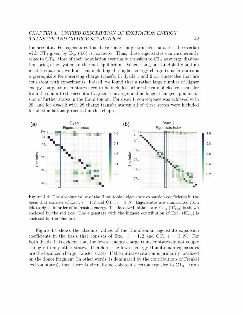
CHAPTER 4. UNIFIED DESCRIPTION OF EXCITATION ENERGYTRANSFER AND CHARGE SEPARATION 42
the acceptor. For eigenstates that have some charge transfer character, the overlapwith CT3 given by Eq. (4.6) is non-zero. Thus, these eigenstates can incoherentlyrelax to CT3. Most of their population eventually transfers to CT3 as energy dissipa-tion brings the system to thermal equilibrium. When using our Lindblad quantummaster equation, we find that including the higher energy charge transfer states isa prerequisite for observing charge transfer in dyads 1 and 2 on timescales that areconsistent with experiments. Indeed, we found that a rather large number of higherenergy charge transfer states need to be included before the rate of electron transferfrom the donor to the acceptor fragment converges and no longer changes upon inclu-sion of further states in the Hamiltonian. For dyad 1, convergence was achieved with20, and for dyad 2 with 28 charge transfer states; all of these states were includedfor all simulations presented in this chapter.
Eigenstate indexExc1
CT3
CT6
CT11
CT16
CT21
Site
inde
x
(a) Dyad 1
0.2
0.4
0.6
0.8
1.0
Eigenstate indexExc1
CT3
CT6
CT11
CT16
CT21
CT26
Site
inde
x(b) Dyad 2
0.2
0.4
0.6
0.8
1.0
Figure 4.4: The absolute value of the Hamiltonian eigenstate expansion coefficients in thebasis that consists of Exci, i = 1, 2 and CTi, i = 3, N . Eigenstates are enumerated fromleft to right, in order of increasing energy. The localized initial state Exc1 (ICexc) is shownenclosed by the red box. The eigenstate with the highest contribution of Exc1 (ICeig) isenclosed by the blue box.
Figure 4.4 shows the absolute values of the Hamiltonian eigenstate expansioncoefficients in the basis that consists of Exci, i = 1, 2 and CTi, i = 3, N . Forboth dyads, it is evident that the lowest energy charge transfer states do not couplestrongly to any other states. Therefore, the lowest energy Hamiltonian eigenstatesare the localized charge transfer states. If the initial excitation is primarily localizedon the donor fragment (in other words, is dominated by the contributions of Frenkelexciton states), then there is virtually no coherent electron transfer to CT3. From
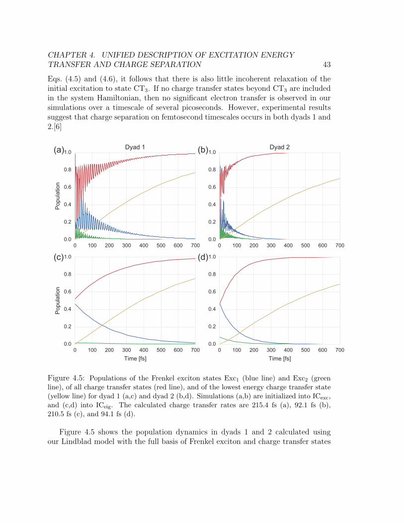
CHAPTER 4. UNIFIED DESCRIPTION OF EXCITATION ENERGYTRANSFER AND CHARGE SEPARATION 43
Eqs. (4.5) and (4.6), it follows that there is also little incoherent relaxation of theinitial excitation to state CT3. If no charge transfer states beyond CT3 are includedin the system Hamiltonian, then no significant electron transfer is observed in oursimulations over a timescale of several picoseconds. However, experimental resultssuggest that charge separation on femtosecond timescales occurs in both dyads 1 and2.[6]
0 100 200 300 400 500 600 7000.0
0.2
0.4
0.6
0.8
1.0
Pop
ulat
ion
(a) Dyad 1
0 100 200 300 400 500 600 7000.0
0.2
0.4
0.6
0.8
1.0(b) Dyad 2
0 100 200 300 400 500 600 700Time [fs]
0.0
0.2
0.4
0.6
0.8
1.0
Pop
ulat
ion
(c)
0 100 200 300 400 500 600 700Time [fs]
0.0
0.2
0.4
0.6
0.8
1.0(d)
Figure 4.5: Populations of the Frenkel exciton states Exc1 (blue line) and Exc2 (greenline), of all charge transfer states (red line), and of the lowest energy charge transfer state(yellow line) for dyad 1 (a,c) and dyad 2 (b,d). Simulations (a,b) are initialized into ICexc,and (c,d) into ICeig. The calculated charge transfer rates are 215.4 fs (a), 92.1 fs (b),210.5 fs (c), and 94.1 fs (d).
Figure 4.5 shows the population dynamics in dyads 1 and 2 calculated usingour Lindblad model with the full basis of Frenkel exciton and charge transfer states
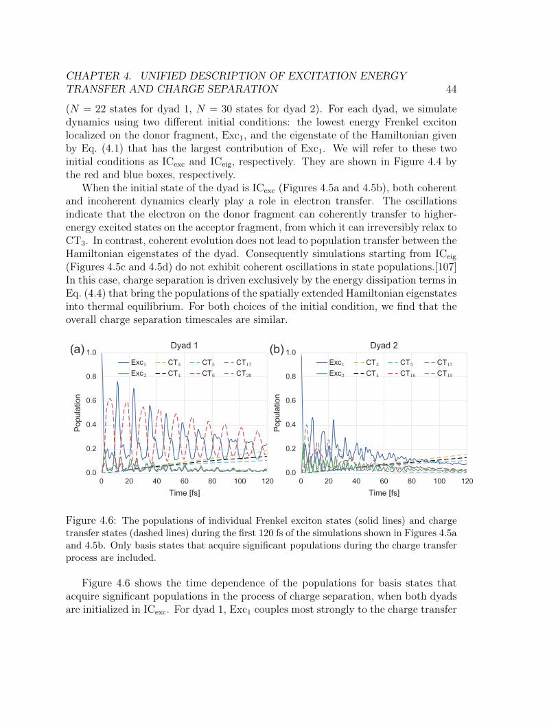
CHAPTER 4. UNIFIED DESCRIPTION OF EXCITATION ENERGYTRANSFER AND CHARGE SEPARATION 44
(N = 22 states for dyad 1, N = 30 states for dyad 2). For each dyad, we simulatedynamics using two different initial conditions: the lowest energy Frenkel excitonlocalized on the donor fragment, Exc1, and the eigenstate of the Hamiltonian givenby Eq. (4.1) that has the largest contribution of Exc1. We will refer to these twoinitial conditions as ICexc and ICeig, respectively. They are shown in Figure 4.4 bythe red and blue boxes, respectively.
When the initial state of the dyad is ICexc (Figures 4.5a and 4.5b), both coherentand incoherent dynamics clearly play a role in electron transfer. The oscillationsindicate that the electron on the donor fragment can coherently transfer to higher-energy excited states on the acceptor fragment, from which it can irreversibly relax toCT3. In contrast, coherent evolution does not lead to population transfer between theHamiltonian eigenstates of the dyad. Consequently simulations starting from ICeig
(Figures 4.5c and 4.5d) do not exhibit coherent oscillations in state populations.[107]In this case, charge separation is driven exclusively by the energy dissipation terms inEq. (4.4) that bring the populations of the spatially extended Hamiltonian eigenstatesinto thermal equilibrium. For both choices of the initial condition, we find that theoverall charge separation timescales are similar.
0 20 40 60 80 100 120Time [fs]
0.0
0.2
0.4
0.6
0.8
1.0
Pop
ulat
ion
(a) Dyad 1
Exc1
Exc2
CT3
CT4
CT5
CT6
CT17
CT20
0 20 40 60 80 100 120Time [fs]
0.0
0.2
0.4
0.6
0.8
1.0
Pop
ulat
ion
(b) Dyad 2
Exc1
Exc2
CT3
CT4
CT5
CT16
CT17
CT19
Figure 4.6: The populations of individual Frenkel exciton states (solid lines) and chargetransfer states (dashed lines) during the first 120 fs of the simulations shown in Figures 4.5aand 4.5b. Only basis states that acquire significant populations during the charge transferprocess are included.
Figure 4.6 shows the time dependence of the populations for basis states thatacquire significant populations in the process of charge separation, when both dyadsare initialized in ICexc. For dyad 1, Exc1 couples most strongly to the charge transfer
CHAPTER 4. UNIFIED DESCRIPTION OF EXCITATION ENERGYTRANSFER AND CHARGE SEPARATION 45
state CT6, as seen in Figure 4.3a. In Figure 4.6a, it is evident that the populationsof Exc1 and CT6 coherently oscillate in counterphase. The magnitudes of theseoscillations decay as energy dissipation redistributes the population from CT6 tothe three lower-energy charge transfer states, CT3, CT4, and CT5. At long times,the populations of all states are given by the Boltzmann distribution, with mostof the population in the lowest charge transfer state, CT3. There is also a secondpathway for charge separation: through the higher-energy Frenkel exciton state,Exc2. Because Frenkel exciton states of the donor are not eigenstates of the dyadHamiltonian, Eq. (4.1), Exc1 has a non-zero coupling to Exc2. Consequently, somepopulation can transfer coherently to this state, and to higher energy charge transferstates that couple strongly to Exc2. For dyad 1, the states most strongly coupled toExc2 are CT17 and CT20. Figure 4.6a shows that these states oscillate in phase withExc2.
The Frenkel exciton states in dyad 2 couple strongly to multiple charge transferstates, resulting in a less straightforward behavior of the coherent oscillations of statepopulations (Figure 4.6b).
We have previously shown in [107] that charge separation is sensitive to therelative timescales of coherent and incoherent dynamics that is determined by theenergy dissipation parameter ν. Using the value of the energy dissipation parameterν = 0.0267 fs, estimated from Ehrenfest-TDDFT simulations, the timescale of chargetransfer is estimated to be 215 fs for dyad 1 and 95 fs for dyad 2. However, regardlessof the value of ν, we find that dyad 2 always exhibits faster charge transfer thandyad 1. This is consistent with the results of transient absorption spectroscopymeasurements of Pillai et al. that found the fastest charge separation on a timescaleof 600 fs for dyad 1, and on a timescale of 200-500 fs for dyad 2.[6]
The difference in relative charge separation timescales for dyads 1 and 2 canbe understood by examining the energy levels and couplings shown in Figure 4.3.The fullerene acceptor in dyad 2 has a denser manifold of charge transfer states atenergies similar to or lower than the initial exciton states; the couplings betweenelectronic and charge transfer states also tend to be larger. Consequently, coherenttransfer between Frenkel exciton states on the donor fragment and higher-energycharge transfer states that, in turn, incoherently transfer population to CT3 is moreefficient in dyad 2 than in dyad 1.
We compare the timescales of charge separation dynamics in dyads 1 and 2 cal-culated using our model to the timescales estimated by using Fermi’s golden rule[7]:
τ−1ij ≈
2π
h|Jij|2
1
|εj − εi|. (4.9)
Here, τ−1ij is the rate of charge transfer between the LUMOs of the donor and the
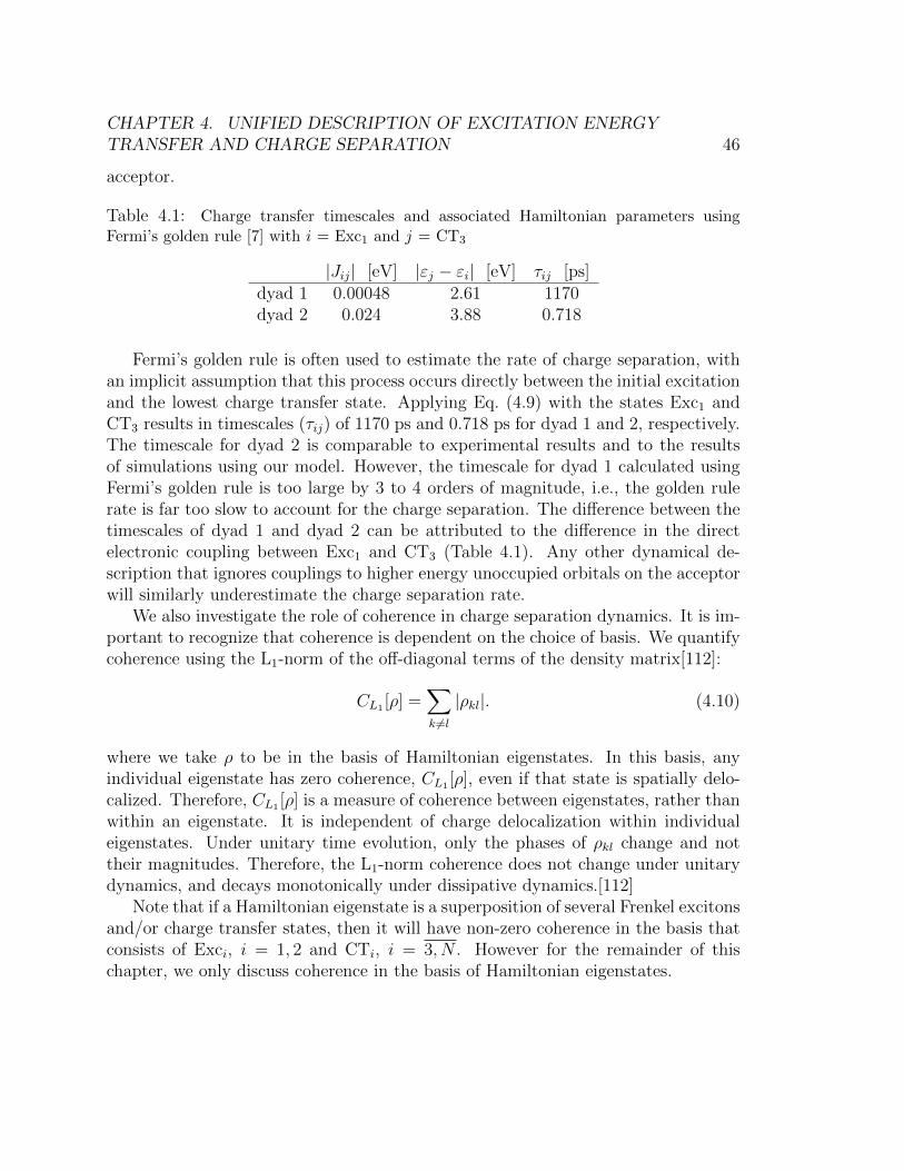
CHAPTER 4. UNIFIED DESCRIPTION OF EXCITATION ENERGYTRANSFER AND CHARGE SEPARATION 46
acceptor.
Table 4.1: Charge transfer timescales and associated Hamiltonian parameters usingFermi’s golden rule [7] with i = Exc1 and j = CT3
|Jij| [eV] |εj − εi| [eV] τij [ps]dyad 1 0.00048 2.61 1170dyad 2 0.024 3.88 0.718
Fermi’s golden rule is often used to estimate the rate of charge separation, withan implicit assumption that this process occurs directly between the initial excitationand the lowest charge transfer state. Applying Eq. (4.9) with the states Exc1 andCT3 results in timescales (τij) of 1170 ps and 0.718 ps for dyad 1 and 2, respectively.The timescale for dyad 2 is comparable to experimental results and to the resultsof simulations using our model. However, the timescale for dyad 1 calculated usingFermi’s golden rule is too large by 3 to 4 orders of magnitude, i.e., the golden rulerate is far too slow to account for the charge separation. The difference between thetimescales of dyad 1 and dyad 2 can be attributed to the difference in the directelectronic coupling between Exc1 and CT3 (Table 4.1). Any other dynamical de-scription that ignores couplings to higher energy unoccupied orbitals on the acceptorwill similarly underestimate the charge separation rate.
We also investigate the role of coherence in charge separation dynamics. It is im-portant to recognize that coherence is dependent on the choice of basis. We quantifycoherence using the L1-norm of the off-diagonal terms of the density matrix[112]:
CL1 [ρ] =∑k 6=l
|ρkl|. (4.10)
where we take ρ to be in the basis of Hamiltonian eigenstates. In this basis, anyindividual eigenstate has zero coherence, CL1 [ρ], even if that state is spatially delo-calized. Therefore, CL1 [ρ] is a measure of coherence between eigenstates, rather thanwithin an eigenstate. It is independent of charge delocalization within individualeigenstates. Under unitary time evolution, only the phases of ρkl change and nottheir magnitudes. Therefore, the L1-norm coherence does not change under unitarydynamics, and decays monotonically under dissipative dynamics.[112]
Note that if a Hamiltonian eigenstate is a superposition of several Frenkel excitonsand/or charge transfer states, then it will have non-zero coherence in the basis thatconsists of Exci, i = 1, 2 and CTi, i = 3, N . However for the remainder of thischapter, we only discuss coherence in the basis of Hamiltonian eigenstates.
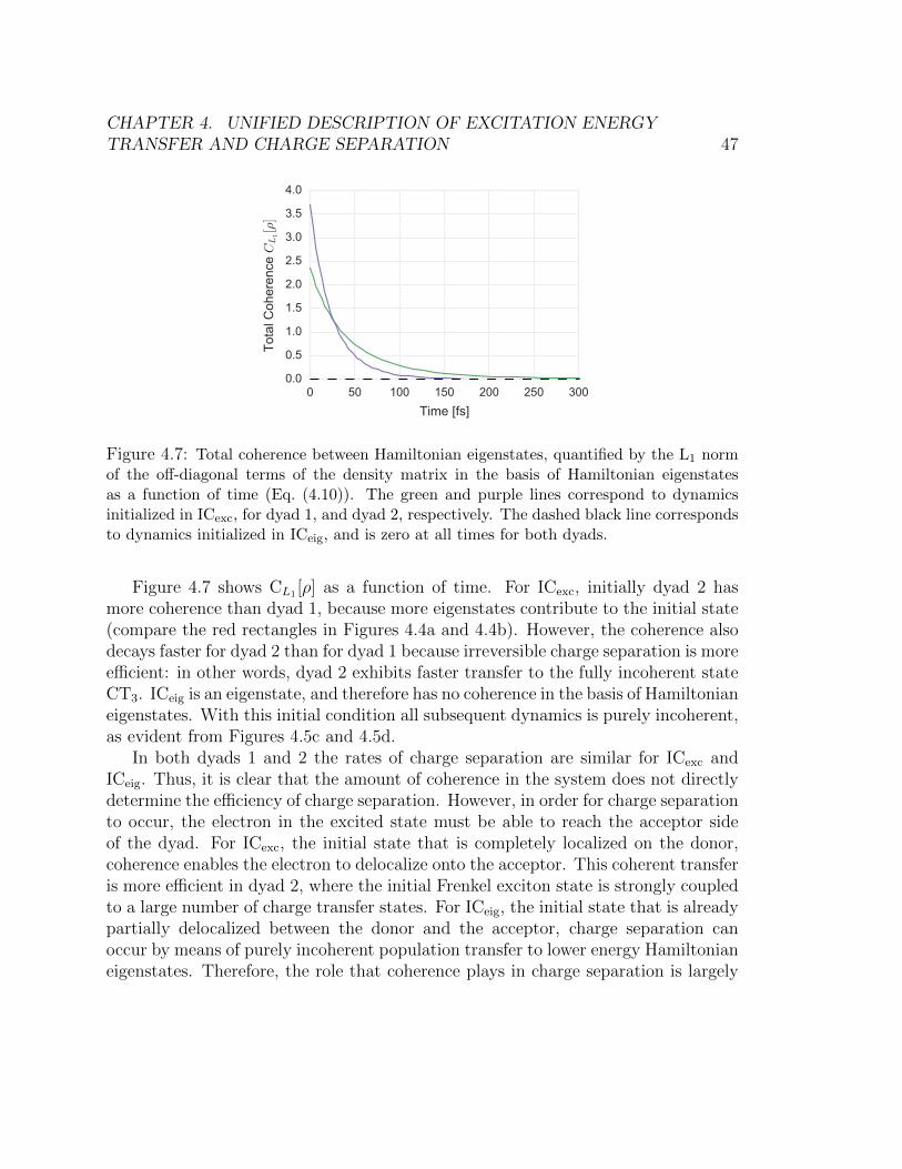
CHAPTER 4. UNIFIED DESCRIPTION OF EXCITATION ENERGYTRANSFER AND CHARGE SEPARATION 47
0 50 100 150 200 250 300Time [fs]
0.0
0.5
1.0
1.5
2.0
2.5
3.0
3.5
4.0
Tota
l Coh
eren
ce C
L1[ρ
]
Figure 4.7: Total coherence between Hamiltonian eigenstates, quantified by the L1 normof the off-diagonal terms of the density matrix in the basis of Hamiltonian eigenstatesas a function of time (Eq. (4.10)). The green and purple lines correspond to dynamicsinitialized in ICexc, for dyad 1, and dyad 2, respectively. The dashed black line correspondsto dynamics initialized in ICeig, and is zero at all times for both dyads.
Figure 4.7 shows CL1 [ρ] as a function of time. For ICexc, initially dyad 2 hasmore coherence than dyad 1, because more eigenstates contribute to the initial state(compare the red rectangles in Figures 4.4a and 4.4b). However, the coherence alsodecays faster for dyad 2 than for dyad 1 because irreversible charge separation is moreefficient: in other words, dyad 2 exhibits faster transfer to the fully incoherent stateCT3. ICeig is an eigenstate, and therefore has no coherence in the basis of Hamiltonianeigenstates. With this initial condition all subsequent dynamics is purely incoherent,as evident from Figures 4.5c and 4.5d.
In both dyads 1 and 2 the rates of charge separation are similar for ICexc andICeig. Thus, it is clear that the amount of coherence in the system does not directlydetermine the efficiency of charge separation. However, in order for charge separationto occur, the electron in the excited state must be able to reach the acceptor sideof the dyad. For ICexc, the initial state that is completely localized on the donor,coherence enables the electron to delocalize onto the acceptor. This coherent transferis more efficient in dyad 2, where the initial Frenkel exciton state is strongly coupledto a large number of charge transfer states. For ICeig, the initial state that is alreadypartially delocalized between the donor and the acceptor, charge separation canoccur by means of purely incoherent population transfer to lower energy Hamiltonianeigenstates. Therefore, the role that coherence plays in charge separation is largely
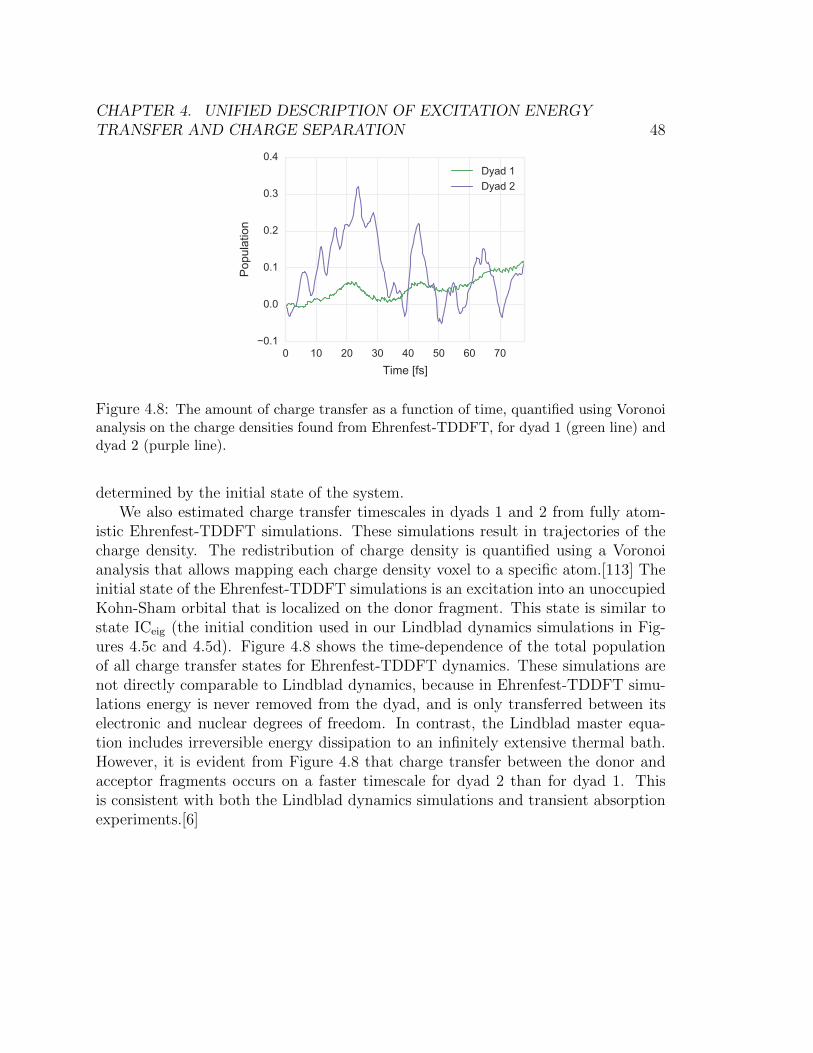
CHAPTER 4. UNIFIED DESCRIPTION OF EXCITATION ENERGYTRANSFER AND CHARGE SEPARATION 48
0 10 20 30 40 50 60 70Time [fs]
0.1
0.0
0.1
0.2
0.3
0.4
Pop
ulat
ion
Dyad 1Dyad 2
Figure 4.8: The amount of charge transfer as a function of time, quantified using Voronoianalysis on the charge densities found from Ehrenfest-TDDFT, for dyad 1 (green line) anddyad 2 (purple line).
determined by the initial state of the system.We also estimated charge transfer timescales in dyads 1 and 2 from fully atom-
istic Ehrenfest-TDDFT simulations. These simulations result in trajectories of thecharge density. The redistribution of charge density is quantified using a Voronoianalysis that allows mapping each charge density voxel to a specific atom.[113] Theinitial state of the Ehrenfest-TDDFT simulations is an excitation into an unoccupiedKohn-Sham orbital that is localized on the donor fragment. This state is similar tostate ICeig (the initial condition used in our Lindblad dynamics simulations in Fig-ures 4.5c and 4.5d). Figure 4.8 shows the time-dependence of the total populationof all charge transfer states for Ehrenfest-TDDFT dynamics. These simulations arenot directly comparable to Lindblad dynamics, because in Ehrenfest-TDDFT simu-lations energy is never removed from the dyad, and is only transferred between itselectronic and nuclear degrees of freedom. In contrast, the Lindblad master equa-tion includes irreversible energy dissipation to an infinitely extensive thermal bath.However, it is evident from Figure 4.8 that charge transfer between the donor andacceptor fragments occurs on a faster timescale for dyad 2 than for dyad 1. Thisis consistent with both the Lindblad dynamics simulations and transient absorptionexperiments.[6]
CHAPTER 4. UNIFIED DESCRIPTION OF EXCITATION ENERGYTRANSFER AND CHARGE SEPARATION 49
4.4 Conclusions
We have simulated the charge separation that follows the optical excitation oftypical donor-acceptor dyads using a perturbative Markovian master equation inLindblad form. The Hamiltonian of the donor-acceptor dyad was constructed usinga basis of Frenkel exciton states on the donor and charge transfer states with theelectron on the acceptor and the hole on the donor, similarly to Ref.[107]. Hamil-tonian parameters were obtained from DFT and TDDFT calculations. The energydissipation parameters in the Lindblad equation were selected to achieve a thermaldistribution of state populations at long times. Additionally, we set the rates ofincoherent population transfer between each pair of states to be proportional to thedegree of spatial overlap between the states involved. This requirement effectivelyassumes that most perturbations of the system that cause incoherent repopulation ofits electronic states occur locally. The rate of energy dissipation was estimated fromEhrenfest-TDDFT molecular dynamics simulations and found to be of the order oftens of femtoseconds.
Because both the electronic coupling and the spatial overlap between an initialexcitation that is primarily localized on the donor and the lowest-energy chargetransfer state are negligible, direct transfer between these states contributes little tothe overall charge separation dynamics. Irreversible charge separation is a processthat involves both coherent and incoherent electron transfer. Within the frameworkof our model, if population is initially excited into the Frenkel exciton state localizedon the donor, it can coherently transfer to higher energy charge transfer states.Concurrently, relaxation from higher to lower-energy charge transfer states occurs.However, for population initially excited into a Hamiltonian eigenstate that is alreadypartially delocalized onto the acceptor, coherent transfer between this and otherHamiltonian eigenstates is not required to achieve charge separation. We foundthat the rate of charge separation is similar for both initial conditions, implyingthat the extent of spatial delocalization of the Hamiltonian eigenstates rather thanthe amount of coherence between eigenstates primarily determines the efficiency ofcharge separation Thus, the importance of coherence in the Hamiltonian eigenstatesfor efficient charge separation depends on the initial state of the system. Note thatspatial delocalization of eigenstates will give rise to coherence in any non-eigenstatebasis, such as the basis consisting of Exci, i = 1, 2 and CTi, i = 3, N .
We have shown that for typical donor-acceptor dyads a large number of chargetransfer states (20 for dyad 1 and 28 for dyad 2) affect the rate of charge separation.Since the higher lying states facilitate charge separation, approximations that neglectthese states will tend to underestimate the rate, sometimes by several orders ofmagnitude. All of these states must be included in the simulation of charge separation
CHAPTER 4. UNIFIED DESCRIPTION OF EXCITATION ENERGYTRANSFER AND CHARGE SEPARATION 50
dynamics to obtain reasonable agreement with both atomistic Ehrenfest-TDDFTmolecular dynamics simulations and charge separation rates obtained from transientabsorption experiments.[6]
In agreement with the experimental results of Pillai et al. [6], in our simulationsthe dyad with a fullerene-based electron acceptor shows higher charge separationrates than the dyad with a porphyrin-based acceptor. We attribute this to theformer acceptor having a larger number of charge transfer states that are close inenergy and are strongly coupled to the lowest two Frenkel exciton states localized onthe donor.
The theoretical analysis presented in this chapter reveals key design criteria thatenable rational selection of donor acceptor pairs for the synthesis of molecular dyadsthat exhibit ultrafast charge separation. First, the donor and acceptor constituentsof the dyad should be chosen to ensure a dense manifold of charge transfer states atenergies close to that of the donor Frenkel exciton. Second, the constituents shouldbe chosen to ensure strong coupling between the donor Frenkel exciton state andthe higher-lying charge transfer states, allowing some extent of delocalization of theHamiltonian eigenstate over both the donor and the acceptor.
51
Chapter 5
Simulations of a prototypicalsynthetic light harvesting system
5.1 Introduction
Light harvesting antennae of photosynthetic organisms are exquisitely organizedbiomolecular structures [114, 115]. Although nearly every photosynthetic specieson the planet has evolved a light harvesting antenna that is customized to its en-vironment, all these antennae are actually composed of relatively few types of pig-ment molecules, e.g., chlorophylls, bacteriochlorophylls, carotenoids, phycobilipro-teins. Two additional factors beyond the choice of pigment are critical in the cus-tomization of the antennae to very different environments. These are the tailoredstructural organization of the pigments, and the tuning of pigment spectral prop-erties by their in-vivo protein environment. In essence, all LHCs are composed ofdensely packed pigments that are usually encased in structure-preserving proteinsand bound to membranes. The dense packing of pigments leads to strong electroniccoupling between chromophores. Some LHCs also have a high degree of organizationthat aligns neighboring dipoles to further enhance electronic coupling. An exampleof this is the LH2 system found in purple bacteria, which consists of pigment-proteincomplexes in which the proteins form helical subunits enclosing rings of 18 and 9pigments [116]. This strong coupling, along with screening from solvent effects af-forded by the binding to photosynthetic membranes, is believed to be the structuralbasis for the long-lived quantum coherent effects recently observed in a number oflight harvesting complexes [2].
Quantum mechanics also plays an important role in the performance of LHCsas antennae for light, both in determining their effective absorption cross-section
CHAPTER 5. SIMULATIONS OF A PROTOTYPICAL SYNTHETIC LIGHTHARVESTING SYSTEM 52
and the excitation energy transfer subsequent to photon absorption. As mentionedabove, the quantum mechanical coupling of several pigments can alter the oscillatorstrength of electronic transitions in pigment-protein complexes. It is believed thatthis is used to advantage to increase the efficiency of light absorption in several LHCs.The most striking example of this comes from green sulfur bacterium, a primitivephotosynthetic organism that lives in extremely low light conditions and possesses ahighly effective antenna structure, the chlorosome, that has recently been identifiedas large concentric nanotubes of tightly packed bacteriochlorophyll molecules [117].This particular structure leads to very strong inter-pigment coupling and greatly en-hanced electronic transition oscillator strengths for efficient light capture and energytransfer. Much of the drive for construction of artificial light harvesting complexesis to design and construct synthetic molecular complexes that mimic these featuresof the chlorosome.
The key to producing synthetic mimics of natural light harvesting systems is theestablishment of the necessary distance relationships between multiple chromophores.Although this could, in principle, be achieved using elaborately designed syntheticmolecules, this approach is typically quite laborious, is difficult to scale, and leads tohighly aromatic systems with poor solubility and limited processing possibilities. Anumber of studies have instead used polymers and dendrimers as scaffold materialsthat establish an upper limit to the distance between chromophores [118, 119], butthese systems generally lack the rigidity needed to control transition dipole orienta-tion and to prevent excimer-based quenching pathways. As an alternative, severalgroups have developed ways to self-assembly of the chromophores themselves, gen-erating large bundles of porphyrins that show energy transfer behavior [120, 121].While these provide interesting chlorosome mimics, it is quite difficult to optimizethe performance of these systems to meet specific applications, since the use of newchromophores with different optical properties can lead to unpredictable assemblyoutcomes. As an alternative, one can employ self-assembling protein coats of virusesas rigid scaffolds that can template the formation of synthetic light harvesting sys-tems [27]. In particular, architectures based on the capsid protein monomer of thetobacco mosaic virus (TMV), can be conveniently produced and employed for theassembly of chromophore arrays by introducing cysteine residues at specific positionsthat allow the covalent attachment of a wide variety of commercially-available chro-mophores with varied optical characteristics. One particularly interesting aspect ofrod-like light harvesting arrays is the fact that they are inherently three-dimensional,and thus could possess redundant energy transfer pathways that could circumventdefect sites better than linear or ring-like systems. An additional advantage of thesynthetic system is that the electronic properties of the aggregate complex can bechemically controlled by changing the type of chromophore, the type of linker used to
CHAPTER 5. SIMULATIONS OF A PROTOTYPICAL SYNTHETIC LIGHTHARVESTING SYSTEM 53
covalently attach the chromophore to the protein, and the position where it attachesto the protein.
In this work we investigate features of the quantum design of synthetic pigment-protein structures for light harvesting that are based on TMV-templated chromophoreassemblies. The close proximity of the chromophores in the TMV assemblies suggeststhat their excited electronic states will be closely coupled. To motivate the design andsynthesis of new systems with enhanced electronic coupling, we analyze here severalpotential synthetic structures using theoretical modeling and spectroscopic charac-terization. We employ molecular mechanics simulations of the chromophore-proteinsystems to provide insight about the geometry and disorder. This is important giventhat these are systems for which crystal structures are hard to obtain, and thus directexperimental information about the geometry is lacking. A key focus of the presentstudy is to understand both the geometry and the mobility of the chromophores,and the extent to which these factors are determined by microscopic details of thesurface of the protein, which typically forces the chromophores to fit into a solvent-accessible pocket. Different chromophores will be oriented differently and can havevarying degrees of mobility depending on their point of linkage and the nature of thelink to the protein. Such geometric and mobility information provides a systematicway to compare and screen for optimal chromophore-protein candidates for synthesisof artificial light-harvesting complexes. The geometry of the chromophores is alsocritical to understanding the optical properties of these aggregate systems, since theelectronic coupling between chromophores is primarily determined by the relativeorientations of their transition dipole moments (TDMs) [5]. In the present work, thegeometries of the conformers found from the molecular mechanics simulations areused in a tight-binding model to simulate the optical properties of the system, withcomparison to experimental spectra.
The remainder of the chapter is constructed as follows. Section 5.2 describesthe TMV and chromophore structures employed here and summarizes the compu-tational methods used for the molecular mechanics structural studies with groundstate chromophores, as well as the ab initio calculations for electronically excitedchromophores and construction of the tight-binding model for simulation of the op-tical spectra. Section 5.3 presents the structural results with analysis of geometry,orientation and ordering of the chromophores, followed by analysis of the linear ab-sorption spectra. Section 5.4 concludes with an assessment of the implications forquantum informed molecular design of artificial light harvesting systems.
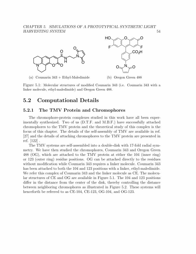
CHAPTER 5. SIMULATIONS OF A PROTOTYPICAL SYNTHETIC LIGHTHARVESTING SYSTEM 54
O ONH
O
N
NO
O
(a) Coumarin 343 + Ethyl-Maledimide
O OHO
F F
N
CO2H
OO
(b) Oregon Green 488
Figure 5.1: Molecular structures of modified Coumarin 343 (i.e. Coumarin 343 with alinker molecule, ethyl-maledimide) and Oregon Green 488.
5.2 Computational Details
5.2.1 The TMV Protein and Chromophores
The chromophore-protein complexes studied in this work have all been exper-imentally synthesized. Two of us (D.T.F. and M.B.F.) have successfully attachedchromophores to the TMV protein and the theoretical study of this complex is thefocus of this chapter. The details of the self-assembly of TMV are available in ref.[27] and the details of attaching chromophores to the TMV protein are presented inref. [122] .
The TMV systems are self-assembled into a double-disk with 17-fold radial sym-metry. We have then studied the chromophores, Coumarin 343 and Oregon Green488 (OG), which are attached to the TMV protein at either the 104 (inner ring)or 123 (outer ring) residue positions. OG can be attached directly to the residueswithout modification while Coumarin 343 requires a linker molecule. Coumarin 343has been attached to both the 104 and 123 positions with a linker, ethyl-maledimide.We refer this complex of Coumarin 343 and the linker molecule as CE. The molecu-lar structures of CE and OG are available in Figure 5.1. The 104 and 123 positionsdiffer in the distance from the center of the disk, thereby controlling the distancebetween neighboring chromophores as illustrated in Figure 5.2. These systems willhenceforth be referred to as CE-104, CE-123, OG-104, and OG-123.
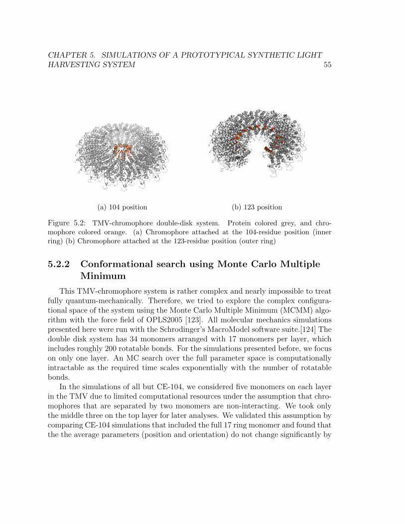
CHAPTER 5. SIMULATIONS OF A PROTOTYPICAL SYNTHETIC LIGHTHARVESTING SYSTEM 55
(a) 104 position (b) 123 position
Figure 5.2: TMV-chromophore double-disk system. Protein colored grey, and chro-mophore colored orange. (a) Chromophore attached at the 104-residue position (innerring) (b) Chromophore attached at the 123-residue position (outer ring)
5.2.2 Conformational search using Monte Carlo MultipleMinimum
This TMV-chromophore system is rather complex and nearly impossible to treatfully quantum-mechanically. Therefore, we tried to explore the complex configura-tional space of the system using the Monte Carlo Multiple Minimum (MCMM) algo-rithm with the force field of OPLS2005 [123]. All molecular mechanics simulationspresented here were run with the Schrodinger’s MacroModel software suite.[124] Thedouble disk system has 34 monomers arranged with 17 monomers per layer, whichincludes roughly 200 rotatable bonds. For the simulations presented before, we focuson only one layer. An MC search over the full parameter space is computationallyintractable as the required time scales exponentially with the number of rotatablebonds.
In the simulations of all but CE-104, we considered five monomers on each layerin the TMV due to limited computational resources under the assumption that chro-mophores that are separated by two monomers are non-interacting. We took onlythe middle three on the top layer for later analyses. We validated this assumption bycomparing CE-104 simulations that included the full 17 ring monomer and found thatthe the average parameters (position and orientation) do not change significantly by
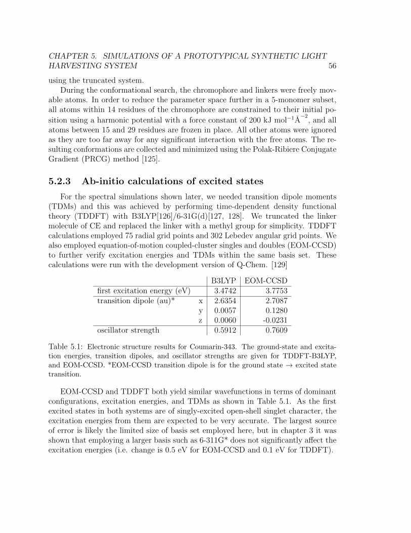
CHAPTER 5. SIMULATIONS OF A PROTOTYPICAL SYNTHETIC LIGHTHARVESTING SYSTEM 56
using the truncated system.During the conformational search, the chromophore and linkers were freely mov-
able atoms. In order to reduce the parameter space further in a 5-monomer subset,all atoms within 14 residues of the chromophore are constrained to their initial po-
sition using a harmonic potential with a force constant of 200 kJ mol−1A−2
, and allatoms between 15 and 29 residues are frozen in place. All other atoms were ignoredas they are too far away for any significant interaction with the free atoms. The re-sulting conformations are collected and minimized using the Polak-Ribiere ConjugateGradient (PRCG) method [125].
5.2.3 Ab-initio calculations of excited states
For the spectral simulations shown later, we needed transition dipole moments(TDMs) and this was achieved by performing time-dependent density functionaltheory (TDDFT) with B3LYP[126]/6-31G(d)[127, 128]. We truncated the linkermolecule of CE and replaced the linker with a methyl group for simplicity. TDDFTcalculations employed 75 radial grid points and 302 Lebedev angular grid points. Wealso employed equation-of-motion coupled-cluster singles and doubles (EOM-CCSD)to further verify excitation energies and TDMs within the same basis set. Thesecalculations were run with the development version of Q-Chem. [129]
B3LYP EOM-CCSDfirst excitation energy (eV) 3.4742 3.7753transition dipole (au)* x 2.6354 2.7087
y 0.0057 0.1280z 0.0060 -0.0231
oscillator strength 0.5912 0.7609
Table 5.1: Electronic structure results for Coumarin-343. The ground-state and excita-tion energies, transition dipoles, and oscillator strengths are given for TDDFT-B3LYP,and EOM-CCSD. *EOM-CCSD transition dipole is for the ground state → excited statetransition.
EOM-CCSD and TDDFT both yield similar wavefunctions in terms of dominantconfigurations, excitation energies, and TDMs as shown in Table 5.1. As the firstexcited states in both systems are of singly-excited open-shell singlet character, theexcitation energies from them are expected to be very accurate. The largest sourceof error is likely the limited size of basis set employed here, but in chapter 3 it wasshown that employing a larger basis such as 6-311G* does not significantly affect theexcitation energies (i.e. change is 0.5 eV for EOM-CCSD and 0.1 eV for TDDFT).
CHAPTER 5. SIMULATIONS OF A PROTOTYPICAL SYNTHETIC LIGHTHARVESTING SYSTEM 57
For the spectral simulation, we used the TDDFT TDMs due to the followingreasons. First, TDDFT calculation is expected to be closer to its complete basisset (CBS) limit as EOM-CCSD calculation is more sensitive to increasing the basisset size. Second, it was pointed by Koch et al. that EOM-CC does not yield size-intensive TDMs, and thus EOM-CC may become a less reliable way to obtain TDMsfor large systems [130]. For these reasons, the analyses requiring TDMs were carriedout based on TDDFT.
5.2.4 Spectral Simulations
Hamiltonian Parametrization
A tight-binding Hamiltonian of the chromophores using the Frenkel Excitonmodel is often used to describe the electronic and optical properties of chromophore-protein systems[14, 29] and we have employed a similar model as well:
H =N∑i=1
εia†i ai +
N∑i=1
N∑j=1
Jij a†i aj (5.1)
where εi is the on-site energy and Jij is the coupling parameter between the site iand the site j. The coupling Jij is a function of the positions of chromophores iand j, and the relative orientations of each of their transition dipole moments. Thisis the same model as described in 3.1. The close proximity between some of thechromophores in our system means that we cannot expect that the commonly usedideal dipole-dipole approximation (IDA) for Jij couplings to hold.
We define ∆Edimern to be the nth electronic excitation energy of the dimer and
∆Emonomern to be the nth electronic excitation energy of the monomer. In the case
of a well-separated dimer, both ∆Edimer1 and ∆Edimer
2 approach to ∆Emonomer1 and
therefore the average of ∆Edimer1 and ∆Edimer
2 is identical to ∆Emonomer1 . However,
our previous work shows that at close distances (< 12 A), the average will beginto deviate from the monomer excitation energy (∆Emonomer
1 ). The extent of thedeviation will depend on the distance and relative orientations of the two interactingchromophores [131].
In order to account for the geometry-dependent effect, we obtain more accurateHamiltonian parameters based on pairwise TDDFT calculations, which are definedas follows:
εi = ∆Emonomer1 +
∑i 6=j
V TDDFT(~Ri, ~µi, ~Rj, ~µj) (5.2)
V TDDFT(~Ri, ~µi, ~Rj, ~µj) =∆Edimer
2 + ∆Edimer1
2−∆Emonomer
1 (5.3)
CHAPTER 5. SIMULATIONS OF A PROTOTYPICAL SYNTHETIC LIGHTHARVESTING SYSTEM 58
Jij = JTDDFT(~Ri, ~µi, ~Rj, ~µj) =Edimer
2 − Edimer1
2(5.4)
where ~Ri denotes the position of the ith chromophore and ~µi denotes the orientationof the ith chromophore.
Among all of our molecular mechanics configurations, there are about 107 pairwiseinteractions. Running a TDDFT calculation for each pairwise interaction in everyconfiguration instance is computationally intractable and also redundant since manyof the pairs will have similar geometries. Our approach is to run a TDDFT calculationat selected distances and orientations and interpolate to predict ab-initio values forother geometries. The precise procedure is as follows:
1. We parametrize the relative orientation of two interacting monomers: r, θA, θB, φBas defined in 3.3b.
2. We then discretize the space along those variables and calculate the TDDFTenergies at the geometries defined by the following grid points: r = [5 A, 5.25A, 5.75 A, 6 A, 6.25 A, 6.5 A, 6.75 A, 7 A, 7.5 A, 8 A, 8.5 A, 9 A, 10 A, 12 A, 14A], θA = [-90◦, 90◦] with a 15◦ increment, θB = [0◦, 180◦] with a 15◦ increment,and φB= [0, 180] with 30◦ increment. Out of the possible 18928 geometries, wediscard the points that yield unphysical geometries, which result in a trainingset of 4456 energies.
3. We employ a model function (see below) with three free parameters each for Jijand Vij, and fit these parameters by using linear regression to match JTDDFT
and V TDDFT, respectively, at each of the grid points.
The model functions used to describe V and J are
Jmodelij (r, θi, θj, φj) = CJ(r)J IDA
ij (r, θi, θj, φj) (5.5)
V modelij (r, θi, θj, φj) = CV (r)V IDA
ij (r, θi, θj, φj) (5.6)
Ck(r) =ck1
(ck2 − exp(r/ck3))(5.7)
where J IDAij and V IDAij are the couplings obtained from IDA, and Ck is a logistic
function, with three free parameters. If CJ and CV deviate significantly from 1,then that is precisely when IDA breaks down. The fitted parameters are found tobe: cV1 = 0.10388804, cV2 = 0.21424357, cV3 = 2.2014798 cJ1 = 0.2889955, cJ2 =1.50871422, cJ3 = 3.14407206.
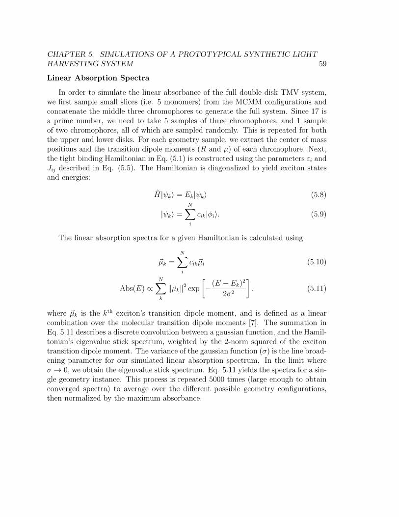
CHAPTER 5. SIMULATIONS OF A PROTOTYPICAL SYNTHETIC LIGHTHARVESTING SYSTEM 59
Linear Absorption Spectra
In order to simulate the linear absorbance of the full double disk TMV system,we first sample small slices (i.e. 5 monomers) from the MCMM configurations andconcatenate the middle three chromophores to generate the full system. Since 17 isa prime number, we need to take 5 samples of three chromophores, and 1 sampleof two chromophores, all of which are sampled randomly. This is repeated for boththe upper and lower disks. For each geometry sample, we extract the center of masspositions and the transition dipole moments (R and µ) of each chromophore. Next,the tight binding Hamiltonian in Eq. (5.1) is constructed using the parameters εi andJij described in Eq. (5.5). The Hamiltonian is diagonalized to yield exciton statesand energies:
H|ψk〉 = Ek|ψk〉 (5.8)
|ψk〉 =N∑i
cik|φi〉. (5.9)
The linear absorption spectra for a given Hamiltonian is calculated using
~µk =N∑i
cik~µi (5.10)
Abs(E) ∝N∑k
‖~µk‖2 exp
[−(E − Ek)2
2σ2
]. (5.11)
where ~µk is the kth exciton’s transition dipole moment, and is defined as a linearcombination over the molecular transition dipole moments [7]. The summation inEq. 5.11 describes a discrete convolution between a gaussian function, and the Hamil-tonian’s eigenvalue stick spectrum, weighted by the 2-norm squared of the excitontransition dipole moment. The variance of the gaussian function (σ) is the line broad-ening parameter for our simulated linear absorption spectrum. In the limit whereσ → 0, we obtain the eigenvalue stick spectrum. Eq. 5.11 yields the spectra for a sin-gle geometry instance. This process is repeated 5000 times (large enough to obtainconverged spectra) to average over the different possible geometry configurations,then normalized by the maximum absorbance.
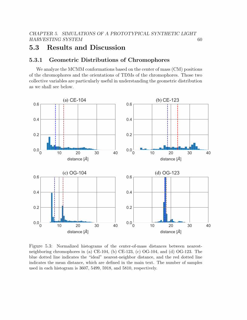
CHAPTER 5. SIMULATIONS OF A PROTOTYPICAL SYNTHETIC LIGHTHARVESTING SYSTEM 60
5.3 Results and Discussion
5.3.1 Geometric Distributions of Chromophores
We analyze the MCMM conformations based on the center of mass (CM) positionsof the chromophores and the orientations of TDMs of the chromophores. Those twocollective variables are particularly useful in understanding the geometric distributionas we shall see below.
(a) (b)
(c) (d)
Figure 5.3: Normalized histograms of the center-of-mass distances between nearest-neighboring chromophores in (a) CE-104, (b) CE-123, (c) OG-104, and (d) OG-123. Theblue dotted line indicates the “ideal” nearest-neighbor distance, and the red dotted lineindicates the mean distance, which are defined in the main text. The number of samplesused in each histogram is 3607, 5499, 5918, and 5810, respectively.
CHAPTER 5. SIMULATIONS OF A PROTOTYPICAL SYNTHETIC LIGHTHARVESTING SYSTEM 61
Figure 5.3 shows a histogram of distances between the CM positions of nearest-neighboring chromophores. We first note that both CE-104 and CE-123 exhibitsignificant multimodal behaviors while bimodal and monomodal behaviors are ob-served for OG-104 and OG-123, respectively. The qualitative difference between CEand OG can be explained simply: the linker molecule in CE allows Coumarin to moveeasily its CM position whereas OG has no linker molecule in our study. We furthercomputed the “ideal” nearest-neighbor distance, rideal, which assumes an equilateral17-polygon, and the mean of nearest-neighbor distances, r. Those two values are notmeaningful in the case of highly multimodal histograms as in the CE cases. In thecase of OG-123, two values are almost identical whereas each of two peaks in OG-104roughly corresponds to rideal and r.
The significance of Figure 5.3 is that some chromophores (in particular CE-104and OG-104) in the TMV systems are not far enough; the distance between nearestneighbors is often less than 12 A. Based on our previous study of Coumarin 343 inchapter 3, when two chromophores are closer than 12 A, it is likely that the usualdipole approximation to the Hamiltonian starts to fail quite catastrophically. Thiswas indeed our motivation to go beyond the dipole approximation, and this will bediscussed further later in this chapter. We note that in the previous study, Coumarinwas considered without a linker molecule. However, we expect the failure of dipoleapproximations to behave similarly. We also expect qualitatively the same conclusionfor OG.
(a) (b)
Figure 5.4: (a) Schematic description of the monomer frame embedded into the entireTMV represented by a disk. The monomer is represented by the wedge. (b) Schematicdescription that represents the polar angle θ and the Azimuthal angle φ in the monomerframe.
CHAPTER 5. SIMULATIONS OF A PROTOTYPICAL SYNTHETIC LIGHTHARVESTING SYSTEM 62
For the purpose of analysis, we introduce the monomer frame illustrated in Fig-ure 5.4. We define the monomer frame as follows: for every chromophore, the x-axispoints towards the center of TMV disk, the z-axis is parallel to the axis of rotationalsymmetry, and the y-axis is defined in the conventional way for given those x- andz-axes (i.e. y = z × x). The radial axis of the polar plot ranges from 0◦ to 180◦, andcorresponds to the polar angle of the monomer frame. The angular axis of the polarplot ranges from 0◦ to 360◦, and corresponds to the azimuthal angle of the monomerframe.
Figure 5.5 shows a histogram of the orientation of TDMs measured in the monomerframe. It shows that the CE systems are more spread than are those in the OG sys-tems. In other words, OG systems are far more confined than CEs. This doesnot necessarily mean that OG systems are more ordered and the quantification oforder-disorder will be discussed later in the chapter. The wider distribution in theCE systems can be understood by considering the effect of the presence of a linkermolecule. We see similar trends in both chromophores when attached to the 104 or123 position. The 104 position exhibits a wider vertical spread compared to the 123position whereas the 123 position shows a wider horizontal spread compared to the104 one. The broad distribution of the CE systems is somewhat surprising given thatthe chromophore molecules are surrounded by the TMV protein environment. Thelinker molecule gives enough flexibility to the Coumarin chromophore which resultsinto a broad geometric distribution. This is one of the reasons that make atomisticsimulations of the system intractable.
5.3.2 Order, Disorder, and Correlation AmongChromophores
We discuss one-body and two-body observables of this system to further quantifythe order and disorder present in the system. There is a simple analogy betweenour system and one-dimensional classical Heisenberg model of 17 sites with periodicboundary conditions. In other words, a TMV disk can be reduced down to a latticewith 17 sites and the chromophore of each monomer can be considered a classicalspin on each site. This analogy allows us to utilize one-body and two-body measuresthat are widely used to quantify order in spin systems. In passing we note that allthe orientation vectors of TDMs used in the following analyses are all normalizedand measured in the monomer frame. As we analyze only five monomers per sample,the periodic boundary condition was not applied throughout the analysis.
The one-body measure considered here is the average of the magnetization of
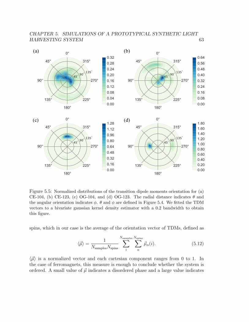
CHAPTER 5. SIMULATIONS OF A PROTOTYPICAL SYNTHETIC LIGHTHARVESTING SYSTEM 63
(a) (b)
(c) (d)
Figure 5.5: Normalized distributions of the transition dipole moments orientation for (a)CE-104, (b) CE-123, (c) OG-104, and (d) OG-123. The radial distance indicates θ andthe angular orientation indicates φ. θ and φ are defined in Figure 5.4. We fitted the TDMvectors to a bivariate gaussian kernel density estimator with a 0.2 bandwidth to obtainthis figure.
spins, which in our case is the average of the orientation vector of TDMs, defined as
〈~µ〉 =1
NsamplesNspins
Nsamples∑i
Nspins∑α
~µα(i). (5.12)
〈~µ〉 is a normalized vector and each cartesian component ranges from 0 to 1. Inthe case of ferromagnets, this measure is enough to conclude whether the system isordered. A small value of ~µ indicates a disordered phase and a large value indicates
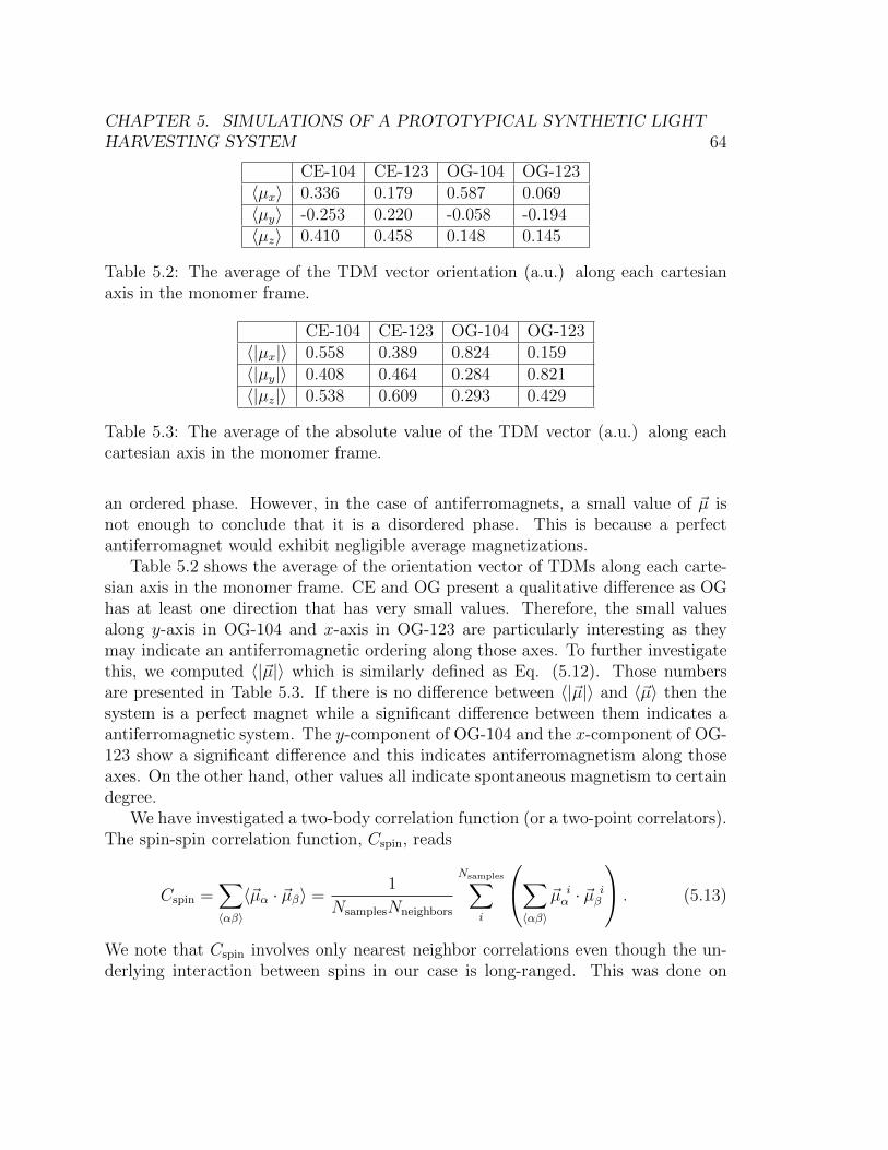
CHAPTER 5. SIMULATIONS OF A PROTOTYPICAL SYNTHETIC LIGHTHARVESTING SYSTEM 64
CE-104 CE-123 OG-104 OG-123〈µx〉 0.336 0.179 0.587 0.069〈µy〉 -0.253 0.220 -0.058 -0.194〈µz〉 0.410 0.458 0.148 0.145
Table 5.2: The average of the TDM vector orientation (a.u.) along each cartesianaxis in the monomer frame.
CE-104 CE-123 OG-104 OG-123〈|µx|〉 0.558 0.389 0.824 0.159〈|µy|〉 0.408 0.464 0.284 0.821〈|µz|〉 0.538 0.609 0.293 0.429
Table 5.3: The average of the absolute value of the TDM vector (a.u.) along eachcartesian axis in the monomer frame.
an ordered phase. However, in the case of antiferromagnets, a small value of ~µ isnot enough to conclude that it is a disordered phase. This is because a perfectantiferromagnet would exhibit negligible average magnetizations.
Table 5.2 shows the average of the orientation vector of TDMs along each carte-sian axis in the monomer frame. CE and OG present a qualitative difference as OGhas at least one direction that has very small values. Therefore, the small valuesalong y-axis in OG-104 and x-axis in OG-123 are particularly interesting as theymay indicate an antiferromagnetic ordering along those axes. To further investigatethis, we computed 〈|~µ|〉 which is similarly defined as Eq. (5.12). Those numbersare presented in Table 5.3. If there is no difference between 〈|~µ|〉 and 〈~µ〉 then thesystem is a perfect magnet while a significant difference between them indicates aantiferromagnetic system. The y-component of OG-104 and the x-component of OG-123 show a significant difference and this indicates antiferromagnetism along thoseaxes. On the other hand, other values all indicate spontaneous magnetism to certaindegree.
We have investigated a two-body correlation function (or a two-point correlators).The spin-spin correlation function, Cspin, reads
Cspin =∑〈αβ〉
〈~µα · ~µβ〉 =1
NsamplesNneighbors
Nsamples∑i
∑〈αβ〉
~µ iα · ~µ i
β
. (5.13)
We note that Cspin involves only nearest neighbor correlations even though the un-derlying interaction between spins in our case is long-ranged. This was done on
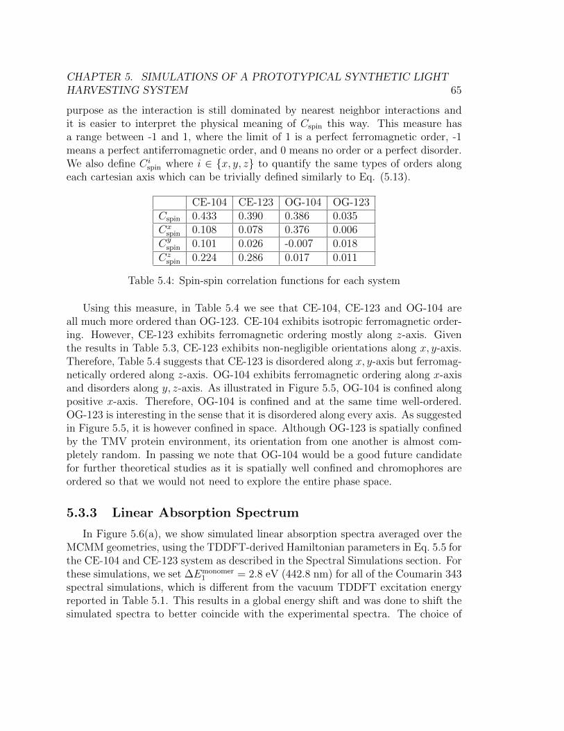
CHAPTER 5. SIMULATIONS OF A PROTOTYPICAL SYNTHETIC LIGHTHARVESTING SYSTEM 65
purpose as the interaction is still dominated by nearest neighbor interactions andit is easier to interpret the physical meaning of Cspin this way. This measure hasa range between -1 and 1, where the limit of 1 is a perfect ferromagnetic order, -1means a perfect antiferromagnetic order, and 0 means no order or a perfect disorder.We also define Ci
spin where i ∈ {x, y, z} to quantify the same types of orders alongeach cartesian axis which can be trivially defined similarly to Eq. (5.13).
CE-104 CE-123 OG-104 OG-123Cspin 0.433 0.390 0.386 0.035Cx
spin 0.108 0.078 0.376 0.006
Cyspin 0.101 0.026 -0.007 0.018
Czspin 0.224 0.286 0.017 0.011
Table 5.4: Spin-spin correlation functions for each system
Using this measure, in Table 5.4 we see that CE-104, CE-123 and OG-104 areall much more ordered than OG-123. CE-104 exhibits isotropic ferromagnetic order-ing. However, CE-123 exhibits ferromagnetic ordering mostly along z-axis. Giventhe results in Table 5.3, CE-123 exhibits non-negligible orientations along x, y-axis.Therefore, Table 5.4 suggests that CE-123 is disordered along x, y-axis but ferromag-netically ordered along z-axis. OG-104 exhibits ferromagnetic ordering along x-axisand disorders along y, z-axis. As illustrated in Figure 5.5, OG-104 is confined alongpositive x-axis. Therefore, OG-104 is confined and at the same time well-ordered.OG-123 is interesting in the sense that it is disordered along every axis. As suggestedin Figure 5.5, it is however confined in space. Although OG-123 is spatially confinedby the TMV protein environment, its orientation from one another is almost com-pletely random. In passing we note that OG-104 would be a good future candidatefor further theoretical studies as it is spatially well confined and chromophores areordered so that we would not need to explore the entire phase space.
5.3.3 Linear Absorption Spectrum
In Figure 5.6(a), we show simulated linear absorption spectra averaged over theMCMM geometries, using the TDDFT-derived Hamiltonian parameters in Eq. 5.5 forthe CE-104 and CE-123 system as described in the Spectral Simulations section. Forthese simulations, we set ∆Emonomer
1 = 2.8 eV (442.8 nm) for all of the Coumarin 343spectral simulations, which is different from the vacuum TDDFT excitation energyreported in Table 5.1. This results in a global energy shift and was done to shift thesimulated spectra to better coincide with the experimental spectra. The choice of
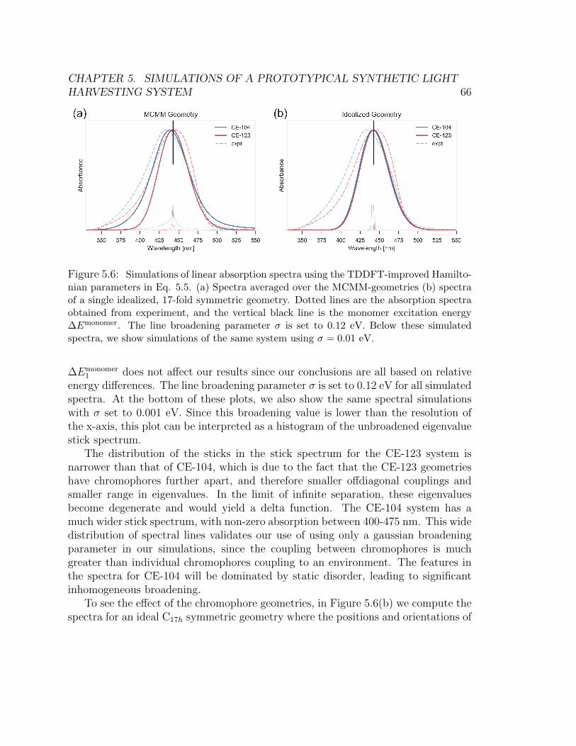
CHAPTER 5. SIMULATIONS OF A PROTOTYPICAL SYNTHETIC LIGHTHARVESTING SYSTEM 66
Figure 5.6: Simulations of linear absorption spectra using the TDDFT-improved Hamilto-nian parameters in Eq. 5.5. (a) Spectra averaged over the MCMM-geometries (b) spectraof a single idealized, 17-fold symmetric geometry. Dotted lines are the absorption spectraobtained from experiment, and the vertical black line is the monomer excitation energy∆Emonomer. The line broadening parameter σ is set to 0.12 eV. Below these simulatedspectra, we show simulations of the same system using σ = 0.01 eV.
∆Emonomer1 does not affect our results since our conclusions are all based on relative
energy differences. The line broadening parameter σ is set to 0.12 eV for all simulatedspectra. At the bottom of these plots, we also show the same spectral simulationswith σ set to 0.001 eV. Since this broadening value is lower than the resolution ofthe x-axis, this plot can be interpreted as a histogram of the unbroadened eigenvaluestick spectrum.
The distribution of the sticks in the stick spectrum for the CE-123 system isnarrower than that of CE-104, which is due to the fact that the CE-123 geometrieshave chromophores further apart, and therefore smaller offdiagonal couplings andsmaller range in eigenvalues. In the limit of infinite separation, these eigenvaluesbecome degenerate and would yield a delta function. The CE-104 system has amuch wider stick spectrum, with non-zero absorption between 400-475 nm. This widedistribution of spectral lines validates our use of using only a gaussian broadeningparameter in our simulations, since the coupling between chromophores is muchgreater than individual chromophores coupling to an environment. The features inthe spectra for CE-104 will be dominated by static disorder, leading to significantinhomogeneous broadening.
To see the effect of the chromophore geometries, in Figure 5.6(b) we compute thespectra for an ideal C17h symmetric geometry where the positions and orientations of
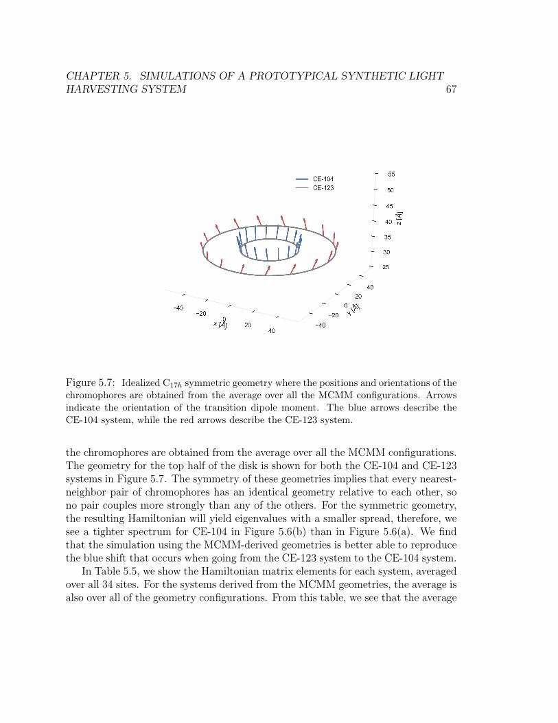
CHAPTER 5. SIMULATIONS OF A PROTOTYPICAL SYNTHETIC LIGHTHARVESTING SYSTEM 67
Figure 5.7: Idealized C17h symmetric geometry where the positions and orientations of thechromophores are obtained from the average over all the MCMM configurations. Arrowsindicate the orientation of the transition dipole moment. The blue arrows describe theCE-104 system, while the red arrows describe the CE-123 system.
the chromophores are obtained from the average over all the MCMM configurations.The geometry for the top half of the disk is shown for both the CE-104 and CE-123systems in Figure 5.7. The symmetry of these geometries implies that every nearest-neighbor pair of chromophores has an identical geometry relative to each other, sono pair couples more strongly than any of the others. For the symmetric geometry,the resulting Hamiltonian will yield eigenvalues with a smaller spread, therefore, wesee a tighter spectrum for CE-104 in Figure 5.6(b) than in Figure 5.6(a). We findthat the simulation using the MCMM-derived geometries is better able to reproducethe blue shift that occurs when going from the CE-123 system to the CE-104 system.
In Table 5.5, we show the Hamiltonian matrix elements for each system, averagedover all 34 sites. For the systems derived from the MCMM geometries, the average isalso over all of the geometry configurations. From this table, we see that the average
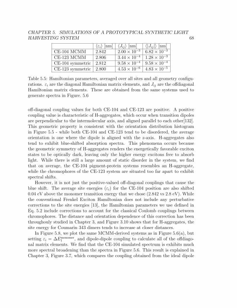
CHAPTER 5. SIMULATIONS OF A PROTOTYPICAL SYNTHETIC LIGHTHARVESTING SYSTEM 68
〈εi〉 [nm] 〈Jij〉 [nm] 〈|Jij|〉 [nm]CE-104 MCMM 2.842 2.00× 10⁻³ 6.82× 10⁻³
CE-123 MCMM 2.806 3.44× 10⁻⁴ 1.28× 10⁻³
CE-104 symmetric 2.812 9.58× 10⁻⁴ 9.58× 10⁻⁴
CE-123 symmetric 2.800 4.53× 10⁻⁶ 4.83× 10⁻⁵
Table 5.5: Hamiltonian parameters, averaged over all sites and all geometry configu-rations. εi are the diagonal Hamiltonian matrix elements, and Jij are the offdiagonalHamiltonian matrix elements. These are obtained from the same systems used togenerate spectra in Figure. 5.6
off-diagonal coupling values for both CE-104 and CE-123 are positive. A positivecoupling value is characteristic of H-aggregates, which occur when transition dipolesare perpendicular to the intermolecular axis, and aligned parallel to each other[132].This geometric property is consistent with the orientation distribution histogramin Figure 5.5 - while both CE-104 and CE-123 tend to be disordered, the averageorientation is one where the dipole is aligned with the z-axis. H-aggregates alsotend to exhibit blue-shifted absorption spectra. This phenomena occurs becausethe geometric symmetry of H-aggregates renders the energetically favorable excitonstates to be optically dark, leaving only the higher energy excitons free to absorblight. While there is still a large amount of static disorder in the system, we findthat on average, the CE-104 pigment-protein systems resembles an H-aggregate,while the chromophores of the CE-123 system are situated too far apart to exhibitspectral shifts.
However, it is not just the positive-valued off-diagonal couplings that cause theblue shift. The average site energies (εi) for the CE-104 position are also shifted0.04 eV above the monomer transition energy that we chose (2.842 vs 2.8 eV). Whilethe conventional Frenkel Exciton Hamiltonian does not include any perturbativecorrections to the site energies [13], the Hamiltonian parameters we use defined inEq. 5.2 include corrections to account for the classical Coulomb couplings betweenchromophores. The distance and orientation dependence of this correction has beenthroughouly studied in Chapter 3, and Figure 3.10 shows that for H-aggregates, thesite energy for Coumarin 343 dimers tends to increase at closer distances.
In Figure 5.8, we plot the same MCMM-derived systems as in Figure 5.6(a), butsetting εi = ∆Emonomer
1 , and dipole-dipole coupling to calculate all of the offdiago-nal matrix elements. We find that the CE-104 simulated spectrum is exhibits muchmore spectral broadening than the spectra in Figure 5.6. This result is explained inChapter 3, Figure 3.7, which compares the coupling obtained from the ideal dipole
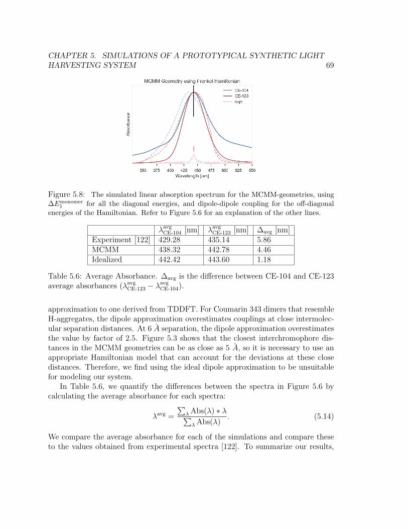
CHAPTER 5. SIMULATIONS OF A PROTOTYPICAL SYNTHETIC LIGHTHARVESTING SYSTEM 69
Figure 5.8: The simulated linear absorption spectrum for the MCMM-geometries, using∆Emonomer
1 for all the diagonal energies, and dipole-dipole coupling for the off-diagonalenergies of the Hamiltonian. Refer to Figure 5.6 for an explanation of the other lines.
λavgCE-104 [nm] λavg
CE-123 [nm] ∆avg [nm]Experiment [122] 429.28 435.14 5.86MCMM 438.32 442.78 4.46Idealized 442.42 443.60 1.18
Table 5.6: Average Absorbance. ∆avg is the difference between CE-104 and CE-123average absorbances (λavg
CE-123 − λavgCE-104).
approximation to one derived from TDDFT. For Coumarin 343 dimers that resembleH-aggregates, the dipole approximation overestimates couplings at close intermolec-ular separation distances. At 6 A separation, the dipole approximation overestimatesthe value by factor of 2.5. Figure 5.3 shows that the closest interchromophore dis-tances in the MCMM geometries can be as close as 5 A, so it is necessary to use anappropriate Hamiltonian model that can account for the deviations at these closedistances. Therefore, we find using the ideal dipole approximation to be unsuitablefor modeling our system.
In Table 5.6, we quantify the differences between the spectra in Figure 5.6 bycalculating the average absorbance for each spectra:
λavg =
∑λ Abs(λ) ∗ λ∑λ Abs(λ)
. (5.14)
We compare the average absorbance for each of the simulations and compare theseto the values obtained from experimental spectra [122]. To summarize our results,
CHAPTER 5. SIMULATIONS OF A PROTOTYPICAL SYNTHETIC LIGHTHARVESTING SYSTEM 70
the experimental spectrum exhibits a blue shift when going from the CE-123 systemto the CE-104 system. While both the simulations using the MCMM geometriesand the idealized geometries exhibit a blue shift, the simulation that incorporatesdisorder is able to match this trend much better. We conclude that the disorder inthe geometry of the CE-104 and CE-123 systems is an important feature of thesesystems, and it is important to account for this disorder in order to model opticalproperties accurately.
5.4 Conclusions
In this work, we present a protocol that generates conformations using a MonteCarlo multiple minima (MCMM) conformation search algorithm, parametrizes asemiempirical tight-binding Hamiltonian based on ab-initio TDDFT calculations andcombines those to generate a linear absorption spectrum that can be directly com-pared to experiments.
In particular, we applied this protocol to study a recently synthesized artificiallight harvesting system consisting of chromophores attached to a tobacco mosaicvirus (TMV) protein. We studied Coumarin 343 (along with a linker) and OregonGreen 488 attached to the 104 and 123 sites on the TMV protein. The resulting foursystems, CE-104, CE-123, OG-104, and OG-123, were studied with MCMM and weobtained a wide array of local minima. We characterized those conformers using theorientation of the transition dipole moment and center-of-mass of dyes attached tothe TMV protein. Such a characterization led to a better understanding of structuralorder and disorder associated with the dyes. CE-104 and CE-123 both exhibit a verybroad geometric distribution, which makes any types of theoretical study more orless intractable. OG-104 and OG-123 are relatively spatially well confined, but OG-123 is more disordered than is OG-104 in terms of the spin-spin correlation functiondiscussed in the main text. For future studies, we believe that OG-104 will be likelythe easiest system to exhaustively study using theoretical methods.
Lastly, we combine the wide array of conformations found through MCMM witha semiempirical tight-binding Hamiltonian to produce a linear absorption spectrumof CE-104 and CE-123. We observed that it is necessary to account for the propergeometric distribution to properly reproduce the blue shift when going from theCE-123 system to the CE-104 system. Despite the high levels of static disorder inthe CE-104 system, our simulations reveal that it exhibits geometric and opticalproperties that resemble an H-aggregate. We find that the typical Frenkel ExcitonHamiltonian with static site energies and dipole-dipole coupling for the offdiagonalelements is insufficient for modeling the optical properties for this system. The
CHAPTER 5. SIMULATIONS OF A PROTOTYPICAL SYNTHETIC LIGHTHARVESTING SYSTEM 71
methods described in this chapter for obtaining more accurate Hamiltonian matrixelements can be used to create a model that better captures the geometric andorientation dependence of these matrix elements, especially at closer intermoleculardistances. While this model is more difficult to use than the dipole approximation,once the model is properly fit, it can efficiently generate tight-binding Hamiltoniansfor arbitrary geometries.
72
Chapter 6
Conclusion
The work presented in this dissertation both evaluates existing models and pro-poses new theoretical models that can be used to simulate the electronic and opticalproperties of chromophore aggregates. The Frenkel exciton model Hamiltonian wasfound to be inadequte in its original formulation when used for the intermolecu-lar distances and orientations found in a prototypical light-harvesting system. Weproposed a modified tight-binding Hamiltonian which performs much better at thecloser intermolecular distances encountered in these photosynthetic systems. Wealso quantified the rate and efficiency of charge separation for a chromophore donor-acceptor system using a Lindblad master equation and a tight-binding model thattreats electronic excitation transfer and charge separation at the same level of theory.The predictions from this model were able to match the trends found in experimentalcharacterizations of the charge separation rate, and we found that it is important toinclude higher energy charge-transfer and exciton states to properly model this sys-tem. We also studied an artificial photosynthetic system that had been synthesizedby attaching chromophores onto the TMV protein. We found that the amount ofstatic disorder in the system is highly dependent on the synthetic choices (choice ofchromophore, protein attachment site). It was necessary to account for this disorderin our model, in addition to using a more accurate tight-binding Hamiltonian, inorder to properly simulate the linear absorbtion spectra for these systems.
6.1 Future Directions
One focus of the work presented in this dissertation was to create models thatwork well for real experimental systems, while balancing efficiency and accuracy.The Frenkel exciton model is often used to model molecular aggregates due to its
CHAPTER 6. CONCLUSION 73
simplicity and ease of use. The approaches that we have presented have an overheadof requiring numerous TDDFT calculations, but once the model is trained on thisdata, the resulting effective Hamiltonian can be created just as efficiently as theFrenkel exciton model Hamiltonian, for arbitrary starting geometries. We suggestthat theoretical studies of photosynthetic systems should consider the assumptionsmade in the Frenkel exciton model, and evaluate whether their system warrents usinga more microscopic treatment of the Hamiltonian.
One future extension of this work would be to combine the techniques for simu-lating charge separation rates and linear absorption presented in ch. 4 and 5 into asingle model. The ability to predict both linear absorption and charge separation ina unified model would be a useful theoretical tool to study artifical photosyntheticsystems that include both a light harvesting component and a charge separation com-ponent. Such a study would be able to screen potential donor acceptor geometries,and discover the tradeoffs between light absorption and charge separation efficencies.
74
References
(1) Blankenship, R. E., Molecular Mechanisms of Photosynthesis ; Blackwell Sci-ence: 2002.
(2) Scholes, G. D. et al. Using coherence to enhance function in chemical andbiophysical systems. Nature 2017, 543, 647–656.
(3) Engel, G. S.; Calhoun, T. R.; Read, E. L.; Ahn, T.-K.; Mancal, T.; Cheng,Y.-C.; Blankenship, R. E.; Fleming, G. R. Evidence for Wavelike EnergyTransfer Through Quantum Coherence in Photosynthetic Systems. Nature2007, 446, 782–6.
(4) Rozzi, C. A.; Falke, S. M.; Spallanzani, N.; Rubio, A.; Molinari, E.; Brida, D.;Maiuri, M.; Cerullo, G.; Schramm, H.; Christoffers, J.; Lienau, C. QuantumCoherence Controls the Charge Separation in a Prototypical Artificial Light-Harvesting System. Nat. Commun. 2013, 4, 1602.
(5) Scholes, G. D.; Fleming, G. R.; Olaya-Castro, A.; van Grondelle, R. LessonsFrom Nature About Solar Light Harvesting. Nat Chem 2011, 3, 763–774.
(6) Pillai, S.; Ravensbergen, J.; Antoniuk-Pablant, A.; Sherman, B. D.; van Gron-delle, R.; Frese, R. N.; Moore, T. a.; Gust, D.; Moore, A. L.; Kennis, J. T. M.Carotenoids as Electron or Excited-State Energy Donors in Artificial Photo-synthesis: an Ultrafast Investigation of a Carotenoporphyrin and a Caroteno-fullerene Dyad. Phys. Chem. Chem. Phys. 2013, 15, 4775–84.
(7) May, V.; Kuhn, O., Charge and Energy Transfer Dynamics in Molecular Sys-tems, 3rd ed.; Wiley-VCH: Weinheim, 2011.
(8) Ishizaki, A.; Calhoun, T. R.; Schlau-Cohen, G. S.; Fleming, G. R. Quantumcoherence and its interplay with protein environments in photosynthetic elec-tronic energy transfer. Physical chemistry chemical physics : PCCP 2010, 12,7319–7337.
(9) Scholes, G. D. Long-range resonance energy transfer in molecular systems.Annual Review of Physical Chemistry 2003, 54, 57–87.
REFERENCES 75
(10) Agranovich, V., Excitations in Organic Solids ; Oxford University Press: 2008.
(11) Knoester, J. In Proceedings of the International School of Physics ”EnricoFermi” Course CXLIX, Agranovich, V. M., LaRocca, G. C., Eds.; Amster-dam: IOS Press: 2002, pp 149–186.
(12) Scholes, G. D.; Ms, C.; Fleming, G. R. In Advances in Chemical Physics,Berry, R. S., Jortner, J., Eds.; Advances in Chemical Physics, Vol. i; JohnWiley & Sons, Inc.: Hoboken, NJ, USA, 2005; Chapter 2, pp 57–129.
(13) Cheng, Y.-C.; Fleming, G. R. Dynamics of Light Harvesting in Photosynthe-sis. Annu. Rev. Phys. Chem. 2009, 60, 241–62.
(14) Van Amerongen, H.; Valkunas, L; van Grondelle, R, Photosynthetic Excitons ;World Scientific: 2000.
(15) Scholes, G. D. Energy Transfer and Spectroscopic Characterization of Multi-chromophoric Assemblies. J. Phys. Chem. 1996, 100, 18731–18739.
(16) Cao, J.; Silbey, R. J. Optimization of Exciton Trapping in Energy TransferProcesses. J. Phys. Chem. A 2009, 113, 13825–38.
(17) Didraga, C.; Klugkist, J. A.; Knoester, J. Optical Properties of Helical Cylin-drical Molecular Aggregates: The Homogeneous Limit. J. Phys. Chem. B2002, 106, 11474–11486.
(18) Didraga, C.; Pugzlys, A.; Hania, P. R.; von Berlepsch, H.; Duppen, K.;Knoester, J.; Pugz, A.; Berlepsch, H. V. Structure, Spectroscopy, and Mi-croscopic Model of Tubular Carbocyanine Dye Aggregates. J. Phys. Chem.B 2004, 108, 14976–14985.
(19) Sarovar, M.; Whaley, K. B. Design Principles and Fundamental Trade-Offsin Biomimetic Light Harvesting. New J. Phys. 2013, 15, 013030.
(20) Scholes, G. D. Quantum-Coherent Electronic Energy Transfer: Did NatureThink of It First? J. Phys. Chem. Lett. 2010, 1, 2–8.
(21) Collini, E.; Wong, C. Y.; Wilk, K. E.; Curmi, P. M. G.; Brumer, P.; Scholes,G. D. Coherently Wired Light-Harvesting in Photosynthetic Marine Algae atAmbient Temperature. Nature 2010, 463, 644–647.
(22) Sarovar, M.; Ishizaki, A.; Fleming, G. R.; Whaley, K. B. Quantum Entan-glement in Photosynthetic Light-Harvesting Complexes. Nat. Phys. 2010, 6,462–467.
(23) Ma, Y.-Z.Y.-Z.; Miller, R. A.; Fleming, G. R.; Francis, M. B. Energy TransferDynamics in Light-Harvesting Assemblies Templated by the Tobacco MosaicVirus Coat Protein. J. Phys. Chem. B 2008, 112, 6887–92.
REFERENCES 76
(24) Klug, A The Tobacco Mosaic Virus Particle: Structure and Assembly. Phil.Trans. R. Soc. B 1999, 354, 531–5.
(25) Endo, M.; Fujitsuka, M.; Majima, T. Porphyrin Light-Harvesting ArraysConstructed in the Recombinant Tobacco Mosaic Virus Scaffold. Chemistry(Weinheim an der Bergstrasse, Germany) 2007, 13, 8660–6.
(26) Nam, Y. S.; Shin, T.; Park, H.; Magyar, A. P.; Choi, K.; Fantner, G.; Nelson,K. A.; Belcher, A. M. Virus-Templated Assembly of Porphyrins into Light-Harvesting Nanoantennae. J. Am. Chem. Soc. 2010, 132, 1462–3.
(27) Miller, R. A.; Presley, A. D.; Francis, M. B. Self-Assembling Light-HarvestingSystems from Synthetically Modified Tobacco Mosaic Virus Coat Proteins.J. Am. Chem. Soc. 2007, 129, 3104–9.
(28) Witus, L. S.; Francis, M. B. Using Synthetically Modified Proteins to MakeNew Materials. Acc. Chem. Res. 2011, 44, 774–83.
(29) Scholes, G. D.; Rumbles, G. Excitons in Nanoscale Systems. Nat. Mater.2006, 5, 683–696.
(30) Krueger, B. P.; Scholes, G. D.; Fleming, G. R. Calculation of Couplings andEnergy-Transfer Pathways between the Pigments of LH2 by the ab InitioTransition Density Cube Method. J. Phys. Chem. B 1998, 102, 5378–5386.
(31) Kasha, M.; Rawls, H. R.; Ashraf El-Bayoumi, M. The Exciton Model inMolecular Spectroscopy. Pure Appl. Chem. 1965, 11, 371–392.
(32) Howard, I. A.; Zutterman, F; Deroover, G; Lamoen, D; Van Alsenoy, C.Approaches to Calculation of Exciton Interaction Energies for a MolecularDimer. J. Phys. Chem. B 2004, 108, 19155–19162.
(33) Munoz Losa, A.; Curutchet, C.; Krueger, B. P.; Hartsell, L. R.; Mennucci, B.Fretting about FRET: Failure of the Ideal Dipole Approximation. Biophys.J. 2009, 96, 4779–88.
(34) Scholes, G. D.; Jordanides, X. J.; Fleming, G. R. Adapting the Forster Theoryof Energy Transfer for Modeling Dynamics in Aggregated Molecular Assem-blies. J. Phys. Chem. B 2001, 105, 1640–1651.
(35) Madjet, M. E.; Abdurahman, a; Renger, T Intermolecular Coulomb Couplingsfrom Ab Initio Electrostatic Potentials: Application to Optical Transitions ofStrongly Coupled Pigments in Photosynthetic Antennae and Reaction Cen-ters. J. Phys. Chem. B 2006, 110, 17268–81.
(36) Hsu, C.-P.; Fleming, G. R.; Head-Gordon, M.; Head-Gordon, T. ExcitationEnergy Transfer in Condensed Media. J. Chem. Phys. 2001, 114, 3065.
REFERENCES 77
(37) Curutchet, C.; Scholes, G. D.; Mennucci, B.; Cammi, R. How Solvent Con-trols Electronic Energy Transfer and Light Harvesting: Toward a Quantum-Mechanical Description of Reaction Field and Screening Effects. J. Phys.Chem. B 2007, 111, 13253–13265.
(38) Sinnokrot, M. O.; Sherrill, C. D. High-Accuracy Quantum Mechanical Studiesof Pi-Pi Interactions in Benzene Dimers. J. Phys. Chem. A 2006, 110, 10656–10668.
(39) Fink, R. F.; Pfister, J; Schneider, A; Zhao, H; Engels, B Ab Initio Configura-tion Interaction Description of Excitation Energy Transfer Between CloselyPacked Molecules. Chem. Phys. 2008, 343, 353–361.
(40) Fink, R. F.; Pfister, J.; Zhao, H. M.; Engels, B. Assessment of QuantumChemical Methods and Basis Sets for Excitation Energy Transfer. Chem.Phys. 2008, 346, 275–285.
(41) Zhao, H. M.; Pfister, J.; Settels, V.; Renz, M.; Kaupp, M.; Dehm, V. C.;Wurthner, F.; Fink, R. F.; Engels, B. Understanding Ground- and Excited-State Properties of Perylene Tetracarboxylic Acid Bisimide Crystals by Meansof Quantum Chemical Computations. J. Am. Chem. Soc. 2009, 131, 15660–15668.
(42) Liu, W.; Settels, V.; Harbach, P. H. P.; Dreuw, A.; Fink, R. F.; Engels, B.Assessment of TD-DFT- and TD-HF-based Approaches for the Predictionof Exciton Coupling Parameters, Potential Energy Curves, and ElectronicCharacters of Electronically Excited Aggregates. J. Comput. Chem. 2011,32, 1971–1981.
(43) Stephens, P. J.; Devlin, F. J.; Chabalowski, C. F.; Frisch, M. J. Ab InitioCalculation of Vibrational Absorption and Circular Dichroism Spectra UsingDensity Functional Force Fields. J. Phys. Chem. 1994, 98, 11623.
(44) Ditchfield, R.; Hehre, W. J.; Pople, J. A. Self-Consistent Molecular-OrbitalMethods. IX. An Extended Gaussian-Type Basis for Molecular-Orbital Stud-ies of Organic Molecules. J. Chem. Phys. 1971, 54, 724.
(45) Hehre, W. J.; Ditchfield, R.; Pople, J. A. Self—Consistent Molecular OrbitalMethods. XII. Further Extensions of Gaussian—Type Basis Sets for Use inMolecular Orbital Studies of Organic Molecules. J. Chem. Phys. 1972, 56,2257.
(46) Hariharan, P.; Pople, J. The Influence of Polarization Functions on MolecularOrbital Hydrogenation Energies. Theo. Chim. Acta 1973, 28, 213.
REFERENCES 78
(47) Runge, E.; Gross, E. K. U. Density-Functional Theory for Time-DependentSystems. Phys. Rev. Lett. 1984, 52, 997.
(48) Gross, E.; Kohn, W. In Density Functional Theory of Many-Fermion Systems,Lowdin, P.-O., Ed.; Adv. Quant. Chem. Vol. 21; Academic Press: 1990, pp 255–291.
(49) Zhao, Y.; Truhlar, D. G. Density Functional for Spectroscopy: No Long-RangeSelf-Interaction Error, Good Performance for Rydberg and Charge-TransferStates, and Better Performance on Average than B3LYP for Ground States.J. Phys. Chem. A 2006, 110, 13126.
(50) Peverati, R.; Truhlar, D. G. Improving the Accuracy of Hybrid Meta-GGADensity Functionals by Range Separation. J. Phys. Chem. Lett. 2011, 2,2810–2817.
(51) Peverati, R.; Truhlar, D. G. M11-L: A Local Density Functional that ProvidesImproved Accuracy for Electronic Structure Calculations in Chemistry andPhysics. J. Phys. Chem. Lett. 2012, 3, 117–124.
(52) Perdew, J. P.; Burke, K.; Ernzerhof, M. Generalized Gradient ApproximationMade Simple. Phys. Rev. Lett. 1996, 77, 3865–3868.
(53) Perdew, J. P.; Burke, K.; Ernzerhof, M. Generalized Gradient ApproximationMade Simple [Phys. Rev. Lett. 77, 3865 (1996)]. Phys. Rev. Lett. 1997, 78,1396–1396.
(54) Clark, T.; Chandrasekhar, J.; Spitznagel, G. W.; Schleyer, P. V. R. EfficientDiffuse Function-Augmented Basis Sets For Anion Calculations. III. The 3-21+G Basis Set for First-Row Elements, Li-F. J. Comput. Chem. 1983, 4,294.
(55) Krishnan, R.; Binkley, J. S.; Seeger, R.; Pople, J. A. Self-Consistent MolecularOrbital Methods. XX. A Basis Set for Correlated Wave Functions. J. Chem.Phys. 1980, 72, 650.
(56) Frisch, M. J.; Pople, J. A.; Binkley, J. S. Self-Consistent Molecular OrbitalMethods 25. Supplementary Functions for Gaussian Basis Sets. J. Chem.Phys. 1984, 80, 3265.
(57) Piecuch, P.; Kucharski, S. A.; Kowalski, K.; Musia l, M. Efficient ComputerImplementation of the Renormalized Coupled-Cluster Methods: The R-CCSD[T],R-CCSD(T), CR-CCSD[T], and CR-CCSD(T) Approaches. Comput. Phys.Commun. 2002, 149, 71.
REFERENCES 79
(58) Kowalski, K.; Piecuch, P. New Coupled-Cluster Methods With Singles, Dou-bles, and Noniterative Triples for High Accuracy Calculations of Excited Elec-tronic States. J. Chem. Phys. 2004, 120, 1715.
(59) Wloch, M.; Gour, J. R.; Kowalski, K.; Piecuch, P. Extension of RenormalizedCoupled-Cluster Methods Including Triple Excitations to Excited ElectronicStates of Open-Shell Molecules. J. Chem. Phys. 2005, 122 214107, 214107.
(60) Ivanic, J.; Ruedenberg, K. Identification of Deadwood in Configuration SpacesThrough General Direct Configuration Interaction. Theo. Chem. Acc. 2001,106, 339.
(61) Cossi, M.; Barone, V. Time-Dependent Density Functional Theory for Moleculesin Liquid Solutions. J. Chem. Phys. 2001, 115, 4708.
(62) Tawada, Y.; Tsuneda, T.; Yanagisawa, S.; Yanai, T.; Hirao, K. A Long-Range-Corrected Time-Dependent Density Functional Theory. J. Chem. Phys. 2004,120, 8425.
(63) Schmidt, M. W.; Baldridge, K. K.; Boatz, J. A.; Elbert, S. T.; Gordon, M. S.;Jensen, J. H.; Koseki, S.; Matsunaga, N.; Nguyen, K. A.; Su, S.; Windus,T. L.; Dupuis, M.; Montgomery, J. A. General Atomic and Molecular Elec-tronic Structure System. J. Comput. Chem. 1993, 14, 1347.
(64) M.S.Gordon; M.W.Schmidt In Theory and Applications of ComputationalChemistry, the First Forty Years, C.E.Dykstra, G.Frenking, K.S.Kim, G.E.Scuseria,Eds.; Elsevier: 2005, p 1167.
(65) Shao, Y. et al. Advances in Methods and Algorithms in a Modern QuantumChemistry Program Package. Phys. Chem. Chem. Phys. 2006, 8, 3172.
(66) Lowdin, P.-O. Quantum Theory of Many-Particle Systems. I. Physical Inter-pretations by Means of Density Matrices, Natural Spin-Orbitals, and Con-vergence Problems in the Method of Configurational Interaction. PhysicalReview 1955, 97, 1474–1489.
(67) Davydov, A. S. The Theory of Molecular Excitons. Sov. Phys. Usp. 1964, 7,145–178.
(68) Agranovich, V. M.; Basko, D. M. Frenkel excitons beyond the Heitler-Londonapproximation. J. Chem. Phys. 2000, 112, 8156–8162.
(69) Mulliken, R. S. Electronic Population Analysis on LCAO[Single Bond]MOMolecular Wave Functions. I. J. Chem. Phys. 1955, 23, 1833.
REFERENCES 80
(70) Madjet, M. E.; Abdurahman, A; Renger, T. Intermolecular Coulomb Cou-plings from Ab Initio Electrostatic Potentials: Application to Optical Transi-tions of Strongly Coupled Pigments in Photosynthetic Antennae and ReactionCenters. J. Phys. Chem. B 2006, 110, 17268–17281.
(71) Muh, F.; Madjet, M. E.; Adolphs, J; Abdurahman, A; Rabenstein, B; Ishikita,H; Knapp, E.-W.; Renger, T. α-Helices Direct Excitation Energy Flow in theFenna-Matthews-Olson Protein. Proc. Nat. Acad. Sc. 2007, 104, 16862.
(72) Dreuw, A.; Head-Gordon, M. Failure of Time-Dependent Density FunctionalTheory for Long-Range Charge-Transfer Excited States: the Zincbacteriochlorin-Bacteriochlorin and Bacteriochlorophyll-Spheroidene Complexes. J. Am. Chem.Soc. 2004, 126, 4007–16.
(73) Pan, F.; Gao, F.; Liang, W.; Zhao, Y. Nature of Low-Lying Excited Statesin H-Aggregated Perylene Bisimide Dyes: Results of TD-LRC-DFT and theMixed Exciton Model. J. Phys. Chem. B 2009, 113, 14581–7.
(74) Novoderezhkin, V. I.; Yakovlev, A. G.; van Grondelle, R.; Shuvalov, V. A.Coherent Nuclear and Electronic Dynamics in Primary Charge Separationin Photosynthetic Reaction Centers: a Redfield Theory Approach. J. Phys.Chem. B 2004, 108, 7445–7457.
(75) Liang, Y.; Xu, Z.; Xia, J.; Tsai, S.-T.; Wu, Y.; Li, G.; Ray, C.; Yu, L. For theBright Future-Bulk Heterojunction Polymer Solar Cells with Power Conver-sion Efficiency of 7.4%. Adv. Mater. 2010, 22, E135–E138.
(76) Lin, Y.; Li, Y.; Zhan, X. Small Molecule Semiconductors for High-EfficiencyOrganic Photovoltaics. Chem. Soc. Rev. 2012, 41, 4245–4272.
(77) Chen, J. D.; Cui, C.; Li, Y. Q.; Zhou, L.; Ou, Q. D.; Li, C.; Li, Y.; Tang,J. X. Single-Junction Polymer Solar Cells Exceeding 10% Power ConversionEfficiency. Adv. Mater. 2015, 27, 1035–1041.
(78) You, J.; Dou, L.; Yoshimura, K.; Kato, T.; Ohya, K.; Moriarty, T.; Emery,K.; Chen, C.-C.; Gao, J.; Li, G.; Yang, Y. Nat. Commun.
(79) Janssen, R. A. J.; Nelson, J. Factors Limiting Device Efficiency in OrganicPhotovoltaics. Adv. Mater. 2013, 25, 1847–1858.
(80) Silinsh, E.; Capek, V., Organic Molecular Crystals: Interaction, Localization,and Transport Phenomena; AIP: Melville, 1994.
(81) Dunlap, W. C.; Watters, R. L. Direct Measurement of the Dielectric Con-stants of Silicon and Germanium. Phys. Rev. 1953, 92, 1396–1397.
REFERENCES 81
(82) Bardeen, C. J. The Structure and Dynamics of Molecular Excitons. Annu.Rev. Phys. Chem. 2014, 65, 127–148.
(83) Knupfer, M Exciton Binding Energies in Organic Semiconductors. Appl. Phys.A 2003, 77, 623–626.
(84) Lakhwani, G.; Rao, A.; Friend, R. H. Bimolecular Recombination in OrganicPhotovoltaics. Annu. Rev. Phys. Chem. 2014, 65, 557–581.
(85) Dennler, G.; Scharber, M. C.; Brabec, C. J. Polymer-Fullerene Bulk-HeterojunctionSolar Cells. Adv. Mater. 2009, 21, 1323–1338.
(86) Jørgensen, M.; Norrman, K.; Krebs, F. C. Stability/Degradation of PolymerSolar Cells. Sol. Energ. Mat. Sol. C. 2008, 92, 686–714.
(87) Gorczak, N.; Tarkuc, S.; Renaud, N.; Houtepen, A. J.; Eelkema, R.; Siebbe-les, L. D. A.; Grozema, F. C. Different Mechanisms for Hole and ElectronTransfer along Identical Molecular Bridges: The Importance of the InitialState Delocalization. J. Phys. Chem. A 2014, 118, 3891–3898.
(88) Iagatti, A.; Cupellini, L.; Biagiotti, G.; Caprasecca, S.; Fedeli, S.; Lapini, A.;Ussano, E.; Cicchi, S.; Foggi, P.; Marcaccio, M.; Mennucci, B.; Di Donato, M.Efficient Photoinduced Charge Separation in a BODIPY-C60 Dyad. J. Phys.Chem. C 2016, 120, 16526–16536.
(89) Liu, L.; Eisenbrandt, P.; Roland, T.; Polkehn, M.; Schwartz, P.-O.; Bruch-los, K.; Omiecienski, B.; Ludwigs, S.; Leclerc, N.; Zaborova, E.; Leonard,J.; Mery, S.; Burghardt, I.; Haacke, S. Controlling Charge Separation andRecombination by Chemical Design in Donor-Acceptor Dyads. Phys. Chem.Chem. Phys. 2016, 18, 18536–18548.
(90) Gelinas, S.; Rao, A.; Kumar, A.; Smith, S. L.; Chin, A. W.; Clark, J.; vander Poll, T. S.; Bazan, G. C.; Friend, R. H. Ultrafast Long-Range ChargeSeparation in Organic Semiconductor Photovoltaic Diodes. Science 2014,343, 512–516.
(91) Kaake, L. G.; Moses, D.; Heeger, A. J. Coherence and Uncertainty in Nanos-tructured Organic Photovoltaics. J. Phys. Chem. Lett. 2013, 4, 2264–2268.
(92) Guo, J.; Ohkita, H.; Benten, H.; Ito, S. Charge Generation and Recombina-tion Dynamics in Poly(3-hexylthiophene)/Fullerene Blend Films with Differ-ent Regioregularities and Morphologies. J. Am. Chem. Soc. 2010, 132, 6154–6164.
(93) Marsh, R. A.; Hodgkiss, J. M.; Albert-Seifried, S.; Friend, R. H. Effect of An-nealing on P3HT:PCBM Charge Transfer and Nanoscale Morphology Probedby Ultrafast Spectroscopy. Nano Lett. 2010, 10, 923–930.
REFERENCES 82
(94) Grancini, G; Maiuri, M; Fazzi, D; Petrozza, A; Egelhaaf, H.-J.; Brida, D;Cerullo, G; Lanzani, G Hot Exciton Dissociation in Polymer Solar Cells.Nat. Mater. 2013, 12, 29–33.
(95) Whaley, K. B.; Kocherzhenko, A. A.; Nitzan, A. Coherent and Diffusive TimeScales for Exciton Dissociation in Bulk Heterojunction Photovoltaic Cells. J.Phys. Chem. C 2014, 118, 27235–27244.
(96) Shen, X.; Han, G.; Fan, D.; Xie, Y.; Yi, Y. Hot Charge-Transfer States Deter-mine Exciton Dissociation in the DTDCTB/C60 Complex for Organic SolarCells: A Theoretical Insight. J. Phys. Chem. C 2015, 119, 11320–11326.
(97) Shao, Y. et al. Advances in Molecular Quantum Chemistry Contained in theQ-Chem 4 Program Package. Mol. Phys. 2015, 113, 184–215.
(98) Maitra, N. T.; Zhang, F.; Cave, R. J.; Burke, K. Double Excitations WithinTime-Dependent Density Functional Theory Linear Response. J. Chem. Phys.2004, 120, 5932–5937.
(99) McHugh, A. J.; Gouterman, M.; Weiss, C. Porphyrins XXIV. Energy, Oscil-lator Strength, and Zeeman Splitting Calculations (SCMO-CI) for Phthalo-cyanine, Porphyrins, and Related Ring Systems. Theor. Chim. Acta 1972,24, 346–370.
(100) Te Velde, G.; Bickelhaupt, F. M.; Baerends, E. J.; Fonseca Guerra, C.; vanGisbergen, S. J. a.; Snijders, J. G.; Ziegler, T. Chemistry with ADF. J. Com-put. Chem. 2001, 22, 931–967.
(101) Senthilkumar, K.; Grozema, F. C.; Bickelhaupt, F. M.; Siebbeles, L. D. A.Charge Transport in Columnar Stacked Triphenylenes: Effects of Conforma-tional Fluctuations on Charge Transfer Integrals and Site Energies. J. Chem.Phys. 2003, 119, 9809.
(102) Wen, S.-H.; Li, A.; Song, J.; Deng, W.-Q.; Han, K.-L.; Goddard, W. A. First-Principles Investigation of Anistropic Hole Mobilities in Organic Semiconduc-tors. J. Phys. Chem. B 2009, 113, 8813–8819.
(103) Kocherzhenko, A. A.; Whaley, K. B.; Sforazzini, G.; Anderson, H. L.; Wykes,M.; Beljonne, D.; Grozema, F. C.; Siebbeles, L. D. A. Effects of the Envi-ronment on Charge Transport in Molecular Wires. J. Phys. Chem. C 2012,116, 25213–25225.
(104) Newton, M. D. Quantum Chemical Probes of Electron-Transfer Kinetics: theNature of Donor-Acceptor Interactions. Chem. Rev. 1991, 91, 767–792.
REFERENCES 83
(105) Ishizaki, A.; Fleming, G. R. Theoretical Examination of Quantum Coherencein a Photosynthetic System at Physiological Temperature. Proc. Natl. Acad.Sci. USA 2009, 106, 17255–17260.
(106) Jesenko, S.; Znidaric, M. Excitation Energy Transfer Efficiency: Equivalenceof Transient and Stationary Setting and the Absence of Non-Markovian Ef-fects. J. Chem. Phys. 2013, 138, 174103.
(107) Kocherzhenko, A. A.; Lee, D.; Forsuelo, M. A.; Whaley, K. B. Coherent andIncoherent Contributions to Charge Separation in Multi-Chromophore Sys-tems. J. Phys. Chem. C 2015, 119, 7590–7603.
(108) Lindblad, G On the Generators of Quantum Dynamical Semigroups. Com-mun. Math. Phys. 1976, 48, 119–130.
(109) Miller, A.; Abrahams, E. Impurity Conduction at Low Concentrations. Phys.Rev. 1960, 120, 745–755.
(110) Castro, A.; Appel, H.; Oliveira, M.; Rozzi, C. A.; Andrade, X.; Lorenzen, F.;Marques, M. A. L.; Gross, E. K. U.; Rubio, A. Octopus: a Tool for the Ap-plication of Time-Dependent Density Functional Theory. Phys. Status SolidiB 2006, 243, 2465–2488.
(111) Perdew, J. P. and Zunger, A. Self-Interaction Correction to Density-FunctionalApproximations for Many-Electron Systems. Phys. Rev. B 1981, 23, 5048–5079.
(112) Baumgratz, T.; Cramer, M.; Plenio, M. B. Quantifying Coherence. Phys. Rev.Lett. 2014, 113, 1–5.
(113) Aurenhammer, F. Voronoi Diagrams—a Survey of a Fundamental GeometricData Structure. ACM Comput. Surv. 1991, 23, 345–405.
(114) Blankenship, R. E., Molecular Mechanisms of Photosynthesis, Second; Chich-ester, UK: Wiley-Blackwell: 2014.
(115) Van Amerongen, H.; Valkunas, L.; Van Grondelle, R., Photosynthetic exci-tons ; World Scientific: 2000.
(116) McDermott, G.; Prince, S.; Freer, A.; Hawthornthwaite-Lawless, A.; Papiz,M.; Cogdell, R.; Isaacs, N. Crystal structure of an integral membrane light-harvesting complex from photosynthetic bacteria. Nature 1995, 374, 517–521.
REFERENCES 84
(117) Ganapathy, S.; Oostergetel, G. T.; Wawrzyniak, P. K.; Reus, M.; Chew,A. G. M.; Buda, F.; Boekema, E. J.; Bryant, D. A.; Holzwarth, A. R.; deGroot, H. J. Alternating syn-anti bacteriochlorophylls form concentric helicalnanotubes in chlorosomes. Proceedings of the National Academy of Sciences2009, 106, 8525–8530.
(118) Gilat, S. L.; Adronov, A.; Frechet, J. M. Light harvesting and energy transferin novel convergently constructed dendrimers. Angewandte Chemie Interna-tional Edition 1999, 38, 1422–1427.
(119) Kim, J.; McQuade, D. T.; Rose, A.; Zhu, Z.; Swager, T. M. Directing en-ergy transfer within conjugated polymer thin films. Journal of the AmericanChemical Society 2001, 123, 11488–11489.
(120) Choi, M.-S.; Yamazaki, T.; Yamazaki, I.; Aida, T. Bioinspired molecular de-sign of light-harvesting multiporphyrin arrays. Angewandte Chemie Interna-tional Edition 2004, 43, 150–158.
(121) Wang, Z.; Medforth, C. J.; Shelnutt, J. A. Porphyrin nanotubes by ionicself-assembly. Journal of the American Chemical Society 2004, 126, 15954–15955.
(122) Finley, D. Synthesis and Development of Viral Capsid Templated Light Har-vesting Systems., PhD, UC Berkeley, 2014, p 110.
(123) Kaminski, G. A.; Friesner, R. A.; Tirado-Rives, J.; Jorgensen, W. L. Eval-uation and reparametrization of the OPLS-AA force field for proteins viacomparison with accurate quantum chemical calculations on peptides. Jour-nal of Physical Chemistry B 2001, 105, 6474–6487.
(124) MacroModel., New York, NY, USA, 2012.
(125) Polak, E.; Ribiere, G. Note sur la convergence de methodes de directionsconjuguees. ESAIM: Mathematical Modelling and Numerical Analysis 1969,DOI: Zbl0174.47906.
(126) Becke, A. D. Density-functional thermochemistry. III. The role of exact ex-change. The Journal of Chemical Physics 1993, 98, 5648–5652.
(127) Petersson, G. A.; Bennett, A.; Tensfeldt, T. G.; Al-Laham, M. A.; Shirley,W. A.; Mantzaris, J. A complete basis set model chemistry. I. The totalenergies of closed-shell atoms and hydrides of the first-row elements. TheJournal of Chemical Physics 1988, 89, 2193–2218.
(128) Petersson, G. A.; Al-Laham, M. A. A complete basis set model chemistry. II.Open-shell systems and the total energies of the first-row atoms. The Journalof Chemical Physics 1991, 94, 6081–6090.
REFERENCES 85
(129) Shao, Y. et al. Advances in molecular quantum chemistry contained in theQ-Chem 4 program package. Mol. Phys. 2015, 113, 184–215.
(130) Koch, H.; Kobayashi, R.; De Meras, A. S.; Jørgensen, P. Calculation of size-intensive transition moments from the coupled cluster singles and doubleslinear response function. The Journal of Chemical Physics 1994, 100, 4393–4400.
(131) Lee, D.; Greenman, L.; Sarovar, M.; Whaley, K. B. Ab initio calculation ofmolecular aggregation effects: A coumarin-343 case study. Journal of PhysicalChemistry A 2013, 117, 11072–11085.
(132) Knoester, J. Modeling the optical properties of excitons in linear and tubularJ-aggregates. International Journal of Photoenergy 2006, 2006, 1–10.