a method for augmenting supersaturated designs - university
TRANSCRIPT
A method for augmenting supersaturated designs
Qiao-Zhen Zhang1, Hong-Sheng Dai2, Min-Qian Liu1∗, Ya Wang3
1 LPMC and Institute of Statistics, Nankai University, Tianjin 300071, China2 Department of Mathematical Sciences, University of Essex, Wivenhoe Park,
Colchester, CO4 3SQ, UK3 State Key Laboratory of Complex Electromagnetic Environment Effects on
Electronics and Information System (CEMEE), Luoyang, 471003, China
Abstract
Initial screening experiments often leave some problems unresolved, adding follow-up
runs is needed to clarify the initial results. In this paper, a technique is developed to add
additional experimental runs to an initial supersaturated design. The added runs are gener-
ated with respect to the Bayesian Ds-optimality criterion and the procedure can incorporate
the model information from the initial design. After analysis of the initial experiment with
several methods, factors are classified into three groups: primary, secondary, and potential
according to the times that they have been identified. The focus is on those secondary factors
since they have been identified several times but not so many that experimenters are sure
that they are active, the proposed Bayesian Ds-optimal augmented design would minimize
the error variances of the parameter estimators of secondary factors. In addition, a blocking
factor will be involved to describe the mean shift between two stages. Simulation results
show that the method performs very well in certain settings.
Keywords: Bayesian D-optimality; Coordinate-exchange algorithm; Follow-up experi-
ment; Sequential design; Supersaturated design.
∗Corresponding author. Email address: [email protected] (Min-Qian Liu).
1

1 Introduction
Screening is the first phase of an experimental study on systems and simulation models.
Its purpose is to eliminate negligible factors so that efforts may be concentrated upon just
the important ones (active factors). Using a supersaturated design (SSD) whose run size is
not enough for estimating all the main effects may be considered when a large experiment is
infeasible in practice. SSDs were introduced by Box (1959), but not studied further until the
appearance of the work by Lin (1993) and Wu (1993). Many developments in the area have
taken place over the last two decades. For further details, please refer to Georgiou (2014),
Sun et al. (2011) and the references therein.
The analysis of SSDs is challenging due to the inherent non-full rank nature of the design
matrix and the fact that the columns of the model matrix are correlated. As a result, the
effects of different factors are aliased with one another making it very difficult to identify the
active factors correctly. Methods to overcome these problems include regression procedures,
such as forward selection (Westfall et al., 1998), stepwise and all-subsets regression (Abraham
et al., 1999), partial least squares methods (Zhang et al., 2007; Yin et al., 2013), shrinkage
methods, including SCAD (Li and Lin, 2002) and Dantzig selector (Phoa et al., 2009) and
Bayesian methods (Beattie et al., 2002; Chen et al., 2011, 2013; Huang et al., 2014). Readers
can refer to Salawu et al. (2015) and Georgiou (2014). However, different methods may give
different results and no method is infallible.
If we want to clarify or confirm initial results and guide the next phase of experimen-
tation, adding follow-up runs to the initial design is a useful way. As a matter of fact,
performing extra experimental runs is the only data-driven way to break confounding pat-
terns and to disentangle confounded effects. Suppose an SSD of n1 runs and k 2-level factors,
denoted by SSD(n1, k), has been run and now the experimenter can afford n2 more runs to
resolve ambiguities, the target is to find the best way to augment the original design to re-
duce uncertainty and get the most information out of the final SSD(n1 +n2, k). Gupta et al.
(2010) considered the problem for 2-level SSDs firstly: E(s2)-optimal designs (proposed by
Booth and Cox, 1962) are augmented with additional runs to create a new class of “extended
2

E(s2)-optimal” designs. Then Gupta et al. (2012) extended the method to s-level designs.
Suen and Das (2010) also used a similar approach to add or remove one row from an existing
E(s2)-optimal design to make a new E(s2)-optimal design. Qin et al. (2015) studied the
optimality of the extended design generated by adding few runs to an existing E(χ2)-optimal
mixed-level SSD and their paper covers the work of Gupta et al. (2010, 2012) as two special
cases. All of these methods, however, did not consider using the information from the initial
analysis and design when adding runs. Gutman et al. (2014) proposed an SSD augmentation
strategy using the Bayesian D-optimality criterion, they considered the information gained
from the initial design, SSD(n1, k), as a prior, and constructed the final SSD(n1 + n2, k) to
reduce the error variances of the parameter estimators under the Bayesian paradigm.
When adding runs to fractional factorial designs, two optimality criteria, D-optimality
and Ds-optimality, are often used. The Ds-optimal design approach would be applied if
the experimenters emphasize precise estimation for the “subset” of the experimental factors.
Kiefer and Wolfowitz (1961) defined a design as Ds-optimal if it minimizes the determinant
of the normalized covariance sub-matrix of estimators of the chosen model parameters while
treating the other parameters as nuisance parameters. The use of Ds-optimality designs
would result in increased power since the parameters of interest are estimated more precisely
(Atkinson and Donev, 1992; Casey et al., 2005). In this paper, we will combine the Ds-
optimality criterion with the Bayesian technique to propose an alternative approach, which
is different from the Bayesian D-optimal augmentation in two aspects: the principle of factor
classification and the optimal criterion.
The next section reviews the relevant background firstly, then we propose the new algo-
rithmic augmentation strategy for SSDs using information from the initial runs in Section 3.
Section 4 compares the performance of the Bayesian Ds-optimal augmented designs with the
Bayesian D-optimal augmented designs by several highlighting examples. Some concluding
remarks are provided in Section 5.
3

2 Bayesian D-optimality and model selection methods
In this section, we briefly review the approach for developing augmenting Bayesian D-
optimal designs in the context of linear models and some model selection methods applied to
SSDs.
2.1 Bayesian D-optimality
Consider the linear model
y = β01n + β1x1 + · · ·+ βkxk + ε = Xβ + ε,
where y is an n×1 vector of observations, β0 is the intercept term, 1n is an n×1 column vector
with all elements unity, xi is an n×1 vector of settings for the ith factor, X is the n×p design
matrix with p = k+1, β is the p×1 vector of coefficients to be estimated, and ε ∼ N(0n, σ2In)
is the noise vector, where 0n is an n × 1 column vector with all elements zero, and In is an
identity matrix of order n. In a two-level factorial design, each factor setting can be coded
as ±1 (or simply ±). Let the prior distribution of the parameters be β | σ2 ∼ N(β0, σ2R−1),
where β0 is the mean of prior distribution for β, R is a prior covariance matrix, and the
conditional distribution of y given β be y | (β, σ2) ∼ N(Xβ, σ2In). Then the posterior
distribution for β given y is
β | y ∼ N(b, σ2(XTX +R)−1),
where b = (XTX +R)−1(XTy +Rβ0).
Let X1 be a model matrix corresponding to the initial n1 runs of an experiment with
response vector y1, and X2 be the additional n2 rows with response vector y2. That is
X =
X1
X2
, y =
y1
y2
.
4

Once the data from the first stage have been collected, many different analysis methods can
be employed to identify active factors and the information from the analysis may be used
as a prior. Gutman et al. (2014) pointed out that the experimenter can classify a factor as
primary term (highlighted by an analysis method or many methods), secondary term (if there
is an indication the factor may be active, but it is not a predominant), or potential term (
with little evidence to suggest it is active). Then prior distributions would be assigned as
follows. Since the primary terms are likely to be active, their coefficients are specified to have
a diffuse prior variance tending to infinity (DuMouchel and Jones, 1994), which implies that
the primary terms are likely to be much different from zero. On the other hand, potential
terms are unlikely to have large effects, and it is proper to assume that they have a relative
small variance. For secondary terms, they may or may not be active, so their prior variances
should be finite, but larger than that for potential terms. We assume that the factors in X
have been reordered after the initial analysis: the intercept and the first p1 − 1 factors are
primary terms, the second p2 factors are potential terms, and the last p3 factors are secondary
terms, where p1 + p2 + p3 = p. Thus the prior covariance matrix R would be
R =
0p1×p1 0p1×p2 0p1×p3
0p2×p1 Ip2/τ2 0p2×p3
0p3×p1 0p3×p2 Ip3/γ2
,
where 0s×t is an s × t matrix with all elements zero, and τ < γ means the secondary terms
are more likely to be active than those potential terms. Using the prior information, the
augmented design SSD(n1+n2, k) is constructed to reduce the error variances of the parameter
estimators under the above Bayesian assumptions for the linear model, that is X2 is chosen
to maximize |XT1 X1 +XT
2 X2 +R| to get a Bayesian D-optimal augmented SSD.
2.2 Model selection methods
We consider four analysis methods here: the half normal plot (Daniel, 1959), the least
absolute shrinkage and selection operator (LASSO) proposed by Tibshirani (1996), the s-
5
moothly clipped absolute deviation (SCAD) by Fan and Li (2001), and the Dantzig selector
(DS) by Candes and Tao (2007).
The half normal plot visually screens factors whose effects seem larger than a random
noise. However, the method may fail to indicate any factor as significantly greater than the
experimental noise (Gupta et al., 2010), so here we list top bk/2c largest effects which are
more likely active than the others, here b·c is the rounding down operation.
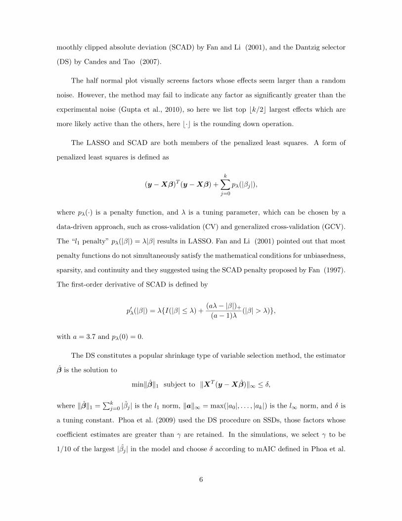
The LASSO and SCAD are both members of the penalized least squares. A form of
penalized least squares is defined as
(y −Xβ)T (y −Xβ) +
k∑j=0
pλ(|βj |),
where pλ(·) is a penalty function, and λ is a tuning parameter, which can be chosen by a
data-driven approach, such as cross-validation (CV) and generalized cross-validation (GCV).
The “l1 penalty” pλ(|β|) = λ|β| results in LASSO. Fan and Li (2001) pointed out that most
penalty functions do not simultaneously satisfy the mathematical conditions for unbiasedness,
sparsity, and continuity and they suggested using the SCAD penalty proposed by Fan (1997).
The first-order derivative of SCAD is defined by
p′λ(|β|) = λ{I(|β| ≤ λ) +(aλ− |β|)+
(a− 1)λ(|β| > λ)},
with a = 3.7 and pλ(0) = 0.
The DS constitutes a popular shrinkage type of variable selection method, the estimator
β̂ is the solution to
min‖β̂‖1 subject to ‖XT (y −Xβ̂)‖∞ ≤ δ,
where ‖β̂‖1 =∑k
j=0 |β̂j | is the l1 norm, ‖a‖∞ = max(|a0|, . . . , |ak|) is the l∞ norm, and δ is
a tuning constant. Phoa et al. (2009) used the DS procedure on SSDs, those factors whose
coefficient estimates are greater than γ are retained. In the simulations, we select γ to be
1/10 of the largest |β̂j | in the model and choose δ according to mAIC defined in Phoa et al.
6

(2009).
In this paper, factors would be classified into primary, potential, secondary groups based
on their identified frequencies and the advices from experts and/or experimenters that would
have a prior claim on the classification. Without the advices, we specify a factor to the
primary group which is considered as active with a high possibility if its identified rate is
no less than 75%. Those factors that have not been identified by any method would be
classified into the potential group, and the other factors whose identified rates belong to
(0, 75%) constitute the secondary group. This principle is a rule of thumb, the threshold is
not immutable and can be adjusted according to the experiences and background knowledge.
The factors in the primary and potential groups are considered as active or inactive with a
high probability, so their active performances are relatively clear compared to the factors in
the secondary group which need more information to clarify.
Remark 1. It is particularly important to point out that the proposed procedure possesses
great flexibility, that means the practitioners can choose the type of analysis methods, the
number of analysis methods and the criteria for classifying factors in terms of their conve-
nience, preference, experience and so on. Here we just select four particular methods to show
how the proposed procedure is carried out.
3 Methodology
For traditional factorial designs, we often consider Ds-optimal and D-optimal design ap-
proach for follow-up experiments. If one is more interested in some parameters, i.e., a “subset”
of regression parameters needs more attention, then using the Ds-optimality criterion may be
a better choice. Therefore, for SSDs, we would combine the Ds-optimality criterion with the
Bayesian technique to give an alternative approach to the Bayesian D-optimal augmentation.
7

3.1 Bayesian Ds-optimality
When analyzing the initial SSD, one may find that different analysis techniques may
identify different sets of active factors, so it is useful to consider the results of several analysis
methods (Lin, 1995). For those factors identified by one or more but not all methods applied,
it is hard to assert that they are active or inactive without further information. The following
example would illustrate some problems when analyzing SSDs.
Example 1. We use the SSD(7,15) presented in Gupta et al. (2010), four active factors are
chosen randomly, and responses would be generated from the equation
y = 5x3 − 10x7 + 2x12 + 8x14 + ε, ε ∼ N(07, I7).
In the model, there are two moderate effects, a large effect and a small one. The design
with responses is given in Table 1. The analysis is challenging since to consider four active
Table 1: E(s2)-optimal SSD(7, 15) presented in Gupta et al. (2010).
Run x1 x2 x3 x4 x5 x6 x7 x8 x9 x10 x11 x12 x13 x14 x15 y
1 −1 1 −1 −1 −1 −1 1 1 1 −1 −1 1 1 −1 −1 −21.473
2 −1 −1 −1 −1 1 −1 −1 1 −1 −1 −1 −1 −1 1 1 11.150
3 −1 1 1 −1 1 1 −1 1 −1 1 1 1 1 1 −1 25.483
4 1 −1 −1 1 −1 −1 −1 −1 −1 1 −1 1 1 1 −1 13.680
5 1 −1 −1 −1 1 1 1 −1 1 1 1 1 −1 −1 1 −22.300
6 −1 1 1 1 −1 −1 −1 −1 1 1 1 −1 −1 −1 1 2.377
7 1 −1 1 1 −1 1 1 1 1 −1 1 −1 1 1 1 0.265
factors may violate the principle of effect sparsity (Box and Meyer, 1986). Marley and Woods
(2010) pointed out that an SSD would likely to be successful under the following conditions,
the factor-to-run ratio is less than two and the number of runs should beyond three times
the number of active factors. Neither conditions holds for the example, however. All results
from the four methods introduced in Section 2.2 are given in Table 2, where the truly active
factors are marked with a superscript “a” and “active factors” identified are indicated with
a “•”.
From Table 2, we can find that each method gives a different result, these four methods
8

Table 2: Analysis of initial SSD(7, 15) data.
Method x1 x2 xa3 x4 x5 x6 xa
7 x8 x9 x10 x11 xa12 x13 xa
14 x15
Half Normal • • • • • • •LASSO • • • • • •SCAD • • • •
DS • • • •
report nine factors of interest. According to the principle of the effect sparsity which tells
that in a large set of factors, relatively few are likely to be active, it is unlikely to assert that
there may have nine active factors. It is satisfying that the true active factors {3, 7, 14} have
been identified by all the four methods. It is disappointing that the active factor 12 has been
deemed as active by only one method (SCAD). In contrast, inactive factor 9 is identified by
three methods out of the four, it is not active at all. So it seems that for a factor, its identified
frequency cannot tell its significance exactly and one needs more information to clarify which
factors are active.
However, we can still get some useful information from the table, for example, factors
{3, 7, 9, 14} may be very likely active since they have been selected as significant by all (or
almost all) the methods. On the other hand, factors {1, 2, 5, 6, 8, 11} may be less likely
active because they have not been identified by any method. For factors {4, 10, 12, 13, 15},
it is not clear whether they are active or not because they have been identified by only
some methods, perhaps some are active and some are not. Based on these results, we can
classify all factors into three groups: primary factors {3, 7, 9, 14} which are very likely to be
active, potential factors {1, 2, 5, 6, 8, 11} which are likely to be inactive, and secondary factors
{4, 10, 12, 13, 15} which cannot be asserted now and need further information to clarify. Such
classification results may be used as prior information for further exploration.
For the situation in Example 1, the immediate concern may be to resolve ambiguities,
that is we want to confirm which factors in {4, 10, 12, 13, 15} are active and which are not.
Adding new runs to the original experiment can provide the necessary information to answer
the question. Inspired by the Ds-optimality, we are more interested in those secondary terms
and want to have an accurate estimate of their regression coefficients which can be achieved
9
by minimizing the variances of these regression coefficients.
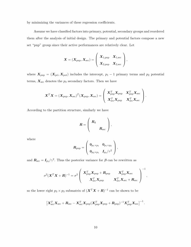
Assume we have classified factors into primary, potential, secondary groups and reordered
them after the analysis of initial design. The primary and potential factors compose a new
set “pnp” group since their active performances are relatively clear. Let
X = (Xpnp,Xsec) =
X1,pnp X1,sec
X2,pnp X2,sec
,
where Xpnp = (Xpri,Xpot) includes the intercept, p1 − 1 primary terms and p2 potential
terms, Xsec denotes the p3 secondary factors. Then we have
XTX = (Xpnp,Xsec)T (Xpnp,Xsec) =
XTpnpXpnp XT
pnpXsec
XTsecXpnp XT
secXsec
.
According to the partition structure, similarly we have
R =
Rd
Rsec
,
where
Rpnp =
0p1×p1 0p1×p2
0p2×p1 Ip2/τ2
,
and Rsec = Ip3/γ2. Thus the posterior variance for β can be rewritten as
σ2(XTX +R)−1 = σ2
XTpnpXpnp +Rpnp XT
pnpXsec
XTsecXpnp XT
secXsec +Rsec
−1
,
so the lower right p3 × p3 submatrix of (XTX +R)−1 can be shown to be
[XT
secXsec +Rsec −XTsecXpnp(XT
pnpXpnp +Rpnp)−1XTpnpXsec
]−1.
10

According to the Ds-optimality, the best choice of X2 is one that maximizes
|XTsecXsec +Rsec −XT
secXpnp(XTpnpXpnp +Rpnp)−1XT
pnpXsec|, (1)
where
XTsecXsec = XT
1,secX1,sec +XT2,secX2,sec,
XTsecXpnp = XT
1,secX1,pnp +XT2,secX2,pnp,
XTpnpXpnp = XT
1,pnpX1,pnp +XT2,pnpX2,pnp.
Similar to Gutman et al. (2014), the final design can be called the Bayesian Ds-optimal
augmented design.
In fact, for Bayesian D-optimality, maximizing |XTX +R| is in some sense equivalent
to minimizing the correlations between all factors under some prior information which is
referred by the matrix R. In addition, with the knowledge of the block matrix, we have
|XTX+R| = |XTpnpXpnp+Rpnp|·|XT
secXsec+Rsec−XTsecXpnp(XT
pnpXpnp+Rpnp)−1XTpnpXsec|,
which is Eq.(1) multiplied by |XTpnpXpnp+Rpnp|. Thus for Bayesian Ds-optimality, it focuses
more attention on the correlations involving secondary factors, the benefit is the reduction in
correlation relating to secondary terms and that would make picking out active factors from
the secondary set be easier.
3.2 Adding a blocking factor
In practice, there could be a long period of time between the original experiment and the
follow up experiment. So it is common to observe a shift in average responses between the
two experiments (Goos et al., 2011). Therefore it would be better to add a term, a blocking
11
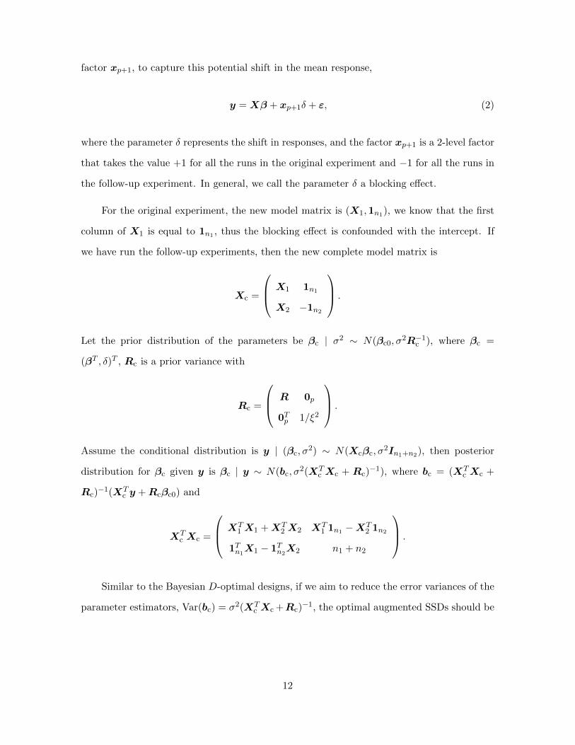
factor xp+1, to capture this potential shift in the mean response,
y = Xβ + xp+1δ + ε, (2)
where the parameter δ represents the shift in responses, and the factor xp+1 is a 2-level factor
that takes the value +1 for all the runs in the original experiment and −1 for all the runs in
the follow-up experiment. In general, we call the parameter δ a blocking effect.
For the original experiment, the new model matrix is (X1,1n1), we know that the first
column of X1 is equal to 1n1 , thus the blocking effect is confounded with the intercept. If
we have run the follow-up experiments, then the new complete model matrix is
Xc =
X1 1n1
X2 −1n2
.
Let the prior distribution of the parameters be βc | σ2 ∼ N(βc0, σ2R−1c ), where βc =
(βT , δ)T , Rc is a prior variance with
Rc =
R 0p
0Tp 1/ξ2
.
Assume the conditional distribution is y | (βc, σ2) ∼ N(Xcβc, σ
2In1+n2), then posterior
distribution for βc given y is βc | y ∼ N(bc, σ2(XT
c Xc + Rc)−1), where bc = (XT
c Xc +
Rc)−1(XT
c y +Rcβc0) and
XTc Xc =
XT1 X1 +XT
2 X2 XT1 1n1 −XT
2 1n2
1Tn1X1 − 1Tn2
X2 n1 + n2
.
Similar to the Bayesian D-optimal designs, if we aim to reduce the error variances of the
parameter estimators, Var(bc) = σ2(XTc Xc +Rc)
−1, the optimal augmented SSDs should be
12

constructed to maximize
|XTc Xc +Rc| =
∣∣∣∣∣∣∣XT
1 X1 +XT2 X2 +R XT
1 1n1 −XT2 1n2 + 0p
1Tn1X1 − 1Tn2
X2 + 0Tp n1 + n2 + 1/ξ2
∣∣∣∣∣∣∣ .Thus, in term of the Bayesian D-optimality, we would maximize
∣∣∣∣XT1 X1 +XT
2 X2 +R− 1
n1 + n2 + 1/ξ2(XT
1 1n1 −XT2 1n2)(1Tn1
X1 − 1Tn2X2)
∣∣∣∣ , (3)
to get X2 generally, since |XTc Xc+Rc| equals Eq.(3) multiplied by (n1+n2+1/ξ2) according
to properties of the block matrix.
When analyzing the augmented design, the blocking factor would be classified as a
secondary term since one cannot detect the blocking effect with the initial design and we are
not sure if there is a mean shift between the two experiments. This is different with Jones
et al. (2008) where they designated the blocking factor as a primary effect. For convenience,
we would set ξ2 = γ2 here. It is easy to consider the Bayesian Ds-optimal augmented SSDs
since we just need to put the blocking factor into the secondary group with an appropriate
adjustment for X and R.
A coordinate-exchange algorithm would be used to construct the optimal augmented
SSDs here, more detailed discussion of the algorithm can be found in Goos et al. (2011).
Example 2. To visually display how a neglected active blocking factor affect the augment-
ed design and the factors’ identification, consider the SSD(7,15) in Table 1 with responses
generated from the equation
y∗ = 5x3 − 10x7 + 2x12 + 8x14 + δx16 + ε, ε ∼ N(07, I7), (4)
where x16 = 1 for the first seven runs and x16 = −1 for the added n2 runs, and δ denotes
the blocking effect. Note that the y∗ in Eq. (4) is a little different from that of Example 1
because we have added a blocking factor here to describe the mean shift between two stages.
However the factors picked out would not change since the mean shift and the former intercept
13

are confounded as a new intercept parameter when analyzing the initial design SSD(7,15).
The factors have been classified into three groups: primary factors 3,7,9,14, potential factors
1,2,5,6,8,11, and the others are secondary factors.
All examples in this paper use γ2 = 100 and τ2 = 5, the same with that of Gutman
et al. (2014). Based on the classification, we use the coordinate-exchange algorithm with
2000 initial random designs to add n2 = 4 runs under the Bayesian Ds-optimality, and the
setting for the number of initial random designs comes from the simulation discussed later.
Ignoring or considering the blocking effect, we get two Bayesian Ds-optimal augmented de-
signs: SSD(11, 15)1 whose added runs are given in the upper part of Table 3 and SSD(11, 15)2
whose added runs are in the lower part of Table 3. Note that for both augmented SSDs, all
settings are the same in the progress of constructing the optimal follow-up runs except that
the blocking factor, x16 = (1, 1, 1, 1, 1, 1, 1,−1,−1,−1,−1)′, has been put in the secondary
group for the latter.
Table 3: Additional 4 Bayesian Ds-optimal runs for the SSD(7, 15).
Run x1 x2 x3 x4 x5 x6 x7 x8 x9 x10 x11 x12 x13 x14 x15 y∗
8 1 1 1 1 −1 1 −1 −1 −1 −1 1 1 −1 1 1 20.190
Ignoring 9 1 −1 −1 1 1 1 1 −1 −1 1 1 −1 −1 −1 −1 −29.880
blocking 10 1 1 1 −1 −1 1 −1 −1 1 −1 1 −1 −1 1 −1 16.751
11 1 1 1 −1 −1 1 −1 −1 −1 1 1 −1 1 1 1 18.222
8 1 −1 1 1 −1 1 1 1 −1 −1 1 1 −1 1 1 2.176
Considering 9 1 −1 1 −1 −1 1 1 1 1 1 1 −1 −1 1 −1 −2.441
blocking 10 −1 1 −1 −1 −1 −1 1 1 −1 1 −1 −1 1 −1 1 −28.052
11 −1 −1 −1 1 1 −1 −1 1 1 1 −1 1 1 1 1 10.244
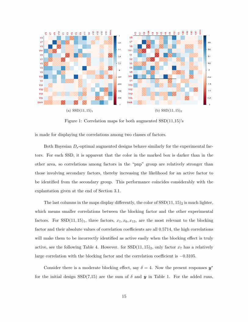
Figure 1 shows the correlation maps for both SSD(11,15)’s. In the figure, “Vi” means
the ith factor for i = 1, . . . , 15 and “block” denotes the blocking factor, in addition, a light
color represents a weak correlation between factors, while a black color represents a high
correlation. To make the graphical representation clear, the diagonal elements have been
set to blank in the figure though their values should be 1. The marked square box in the
diagram corresponds to the “pnp” group including primary and potential factors, secondary
and blocking factors stand back, the order is the same with the above. Such an arrangement
14
(a) SSD(11, 15)1 (b) SSD(11, 15)2
Figure 1: Correlation maps for both augmented SSD(11,15)’s
is made for displaying the correlations among two classes of factors.
Both Bayesian Ds-optimal augmented designs behave similarly for the experimental fac-
tors. For each SSD, it is apparent that the color in the marked box is darker than in the
other area, so correlations among factors in the “pnp” group are relatively stronger than
those involving secondary factors, thereby increasing the likelihood for an active factor to
be identified from the secondary group. This performance coincides considerably with the
explantation given at the end of Section 3.1.
The last columns in the maps display differently, the color of SSD(11, 15)2 is much lighter,
which means smaller correlations between the blocking factor and the other experimental
factors. For SSD(11, 15)1, three factors, x1, x6, x13, are the most relevant to the blocking
factor and their absolute values of correlation coefficients are all 0.5714, the high correlations
will make them to be incorrectly identified as active easily when the blocking effect is truly
active, see the following Table 4. However. for SSD(11, 15)2, only factor x7 has a relatively
large correlation with the blocking factor and the correlation coefficient is −0.3105.
Consider there is a moderate blocking effect, say δ = 4. Now the present responses y∗
for the initial design SSD(7,15) are the sum of δ and y in Table 1. For the added runs,
15
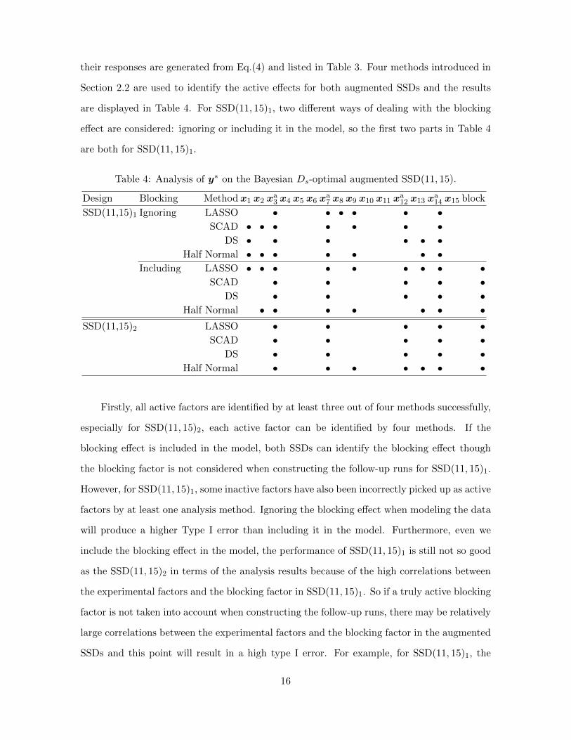
their responses are generated from Eq.(4) and listed in Table 3. Four methods introduced in
Section 2.2 are used to identify the active effects for both augmented SSDs and the results
are displayed in Table 4. For SSD(11, 15)1, two different ways of dealing with the blocking
effect are considered: ignoring or including it in the model, so the first two parts in Table 4
are both for SSD(11, 15)1.
Table 4: Analysis of y∗ on the Bayesian Ds-optimal augmented SSD(11, 15).
Design Blocking Method x1 x2 xa3 x4 x5 x6 x
a7 x8 x9 x10 x11 x
a12 x13 x
a14 x15 block
SSD(11,15)1 Ignoring LASSO • • • • • •SCAD • • • • • • •
DS • • • • • •Half Normal • • • • • • •
Including LASSO • • • • • • • • •SCAD • • • • •
DS • • • • •Half Normal • • • • • • •
SSD(11,15)2 LASSO • • • • •SCAD • • • • •
DS • • • • •Half Normal • • • • • • •
Firstly, all active factors are identified by at least three out of four methods successfully,
especially for SSD(11, 15)2, each active factor can be identified by four methods. If the
blocking effect is included in the model, both SSDs can identify the blocking effect though
the blocking factor is not considered when constructing the follow-up runs for SSD(11, 15)1.
However, for SSD(11, 15)1, some inactive factors have also been incorrectly picked up as active
factors by at least one analysis method. Ignoring the blocking effect when modeling the data
will produce a higher Type I error than including it in the model. Furthermore, even we
include the blocking effect in the model, the performance of SSD(11, 15)1 is still not so good
as the SSD(11, 15)2 in terms of the analysis results because of the high correlations between
the experimental factors and the blocking factor in SSD(11, 15)1. So if a truly active blocking
factor is not taken into account when constructing the follow-up runs, there may be relatively
large correlations between the experimental factors and the blocking factor in the augmented
SSDs and this point will result in a high type I error. For example, for SSD(11, 15)1, the
16

inactive factors x1 has been selected as active incorrectly by three out of four methods, note
the correlation coefficient between it and the blocking factor is 0.5714, another correlated
inactive factor x13 has also been selected as active by two methods.
4 Simulation studies and results
In the section, simulations are carried out to study the performance of two classes of
augmented Bayesian D-optimal and Bayesian Ds-optimal SSDs, some comparisons are also
made.
4.1 Features varied
We vary the following simulation settings in our study.
1. Factor-to-run ratios in the SSDs. Three choices of decreasing difficulty would be used:
SSD(7,15), SSD(8,13) and SSD(9,12), with the ratios varying from 2.14 to 1.33. Three
initial SSDs are all E(s2)-optimal designs, where the first two come from Gutman et
al. (2014) and the last one is constructed using the nonorthogonal array algorithm of
Nguyen (1996) in Gendex (http://www.designcomputing.net/gendex/). The reason
to consider such SSDs with few runs is that the commonly used methods do not perform
well for these designs, so there may be an urgent need to add trials to clarify which
factors are active.
2. Experimental scenarios. We vary the number and magnitude of active factors over
three scenarios. Specifically, the magnitude of the regression coefficient for each of the
a active factors and one blocking factor is drawn from N(µ, 1), with different scenarios
of :
(1) a = 3, µ = 5; (2) a = 4, µ = 4; (3) a = 5, µ = 3.
3. Design augmenting criteria. Here we include the Bayesian D-optimal and the new
Bayesian Ds-optimal augmented SSDs.
17

4. The number of added runs n2. We choose to add n2 = 2, 3, . . . , k+1−n1 follow-up runs,
the augmented design would not be supersaturated any more when n2 > k + 1− n1.
5. The Bayesian D-optimal and Bayesian Ds-optimal augmented SSDs are all generated
using coordinate-exchange algorithm with M random starts.
We have made a number of simulations to find how many random-start designs would
present an optimal or near optimal augmented SSDs, i.e., the values of the optimal criterion
in Eq.(1) (or Eq.(3)) would have no or very small difference. As expected, an appropriate
choice is related to the number of added runs, the number of factors, and the classification
of factors. For instance, in Example 2, when one run is added, 50 random starts are enough
to give a Bayesian Ds-optimal augmented SSD(7+1,15) since the results with M = 50 and
the results with M = 500 are the same. However, when adding n2 = 3 runs, there are some
differences in the values of criterion (1), even we choose 100 random starts. A large number
of simulations show that the the criterion value is relatively stable only when M is around or
above 1000. As the number of added runs increases, the value of Eq.(1) increases gradually,
meanwhile, much more start designs are needed to get an optimal or near optimal augmented
SSD. However, in general, when n2 is larger, even if the values of Eq.(1) (or Eq.(3)) are
slightly different for two augmented SSDs, the impact on the latter data analysis is very
small. Thus we set M = dn2/2e ∗ 1000, where d·e is for rounding up, and it would present a
near optimal augmented SSD based on our simulation results.
In each of the 1000 iterations:
1. Among the 2nd, 3rd, . . ., k+1th columns of X, a columns are randomly assigned as the
active experimental factors. Their coefficients β and the coefficient δ for the blocking
factor are obtained by sampling from N(µ, 1) and randomly assigning signs (+ or −).
2. For simplicity, the remaining k−a columns (inactive effects) are assigned to be exactly
zero.
3. The response vector is generated from the model in Eq.(2) with error ε ∼ N(0n1 , In1).
4. All factors would be classified into their appropriate groups in terms of the classifying
18

principle after being analyzed by four model selection methods introduced in Section
2.2. The blocking factor is assigned as secondary term.
5. Add n2 runs by maximizing the objective functions in Eq.(1) and Eq.(3) to get the
Bayesian Ds-optimal and the Bayesian D-optimal augmented SSDs respectively.
6. Generate the new responses for the added n2 runs. Analyze the final augmented SSDs
with four model selection methods. Then those factors (identified as active by at least
three methods here) classified into the primary group are the declared “active” factors
now.
4.2 Simulation results for augmenting SSDs
Three different criteria similar to Marley and Woods (2010) would be used to assess the
performance of the augmented designs.
Power: The average proportion of active factors classified into the primary group.
Type I error: The average proportion of the inactive factors classified into the primary
group.
Coverage: The average proportion of times that all the truly active effects are classified
into the primary group.
Clearly, Power and Coverage are the-larger-the-better, and Type I error is the-smaller-the-
better. Figures 2–4 show the Power, Type I error and Coverage for three SSDs, respectively.
For the SSD(7 + n2,15), Figure 2 shows the dominance of the Bayesian Ds-optimal
augmented SSDs with regard to Power, where the superiority is particularly evident when
adding fewer runs. For example, in the first scenario, a = 3, µ = 5, when n2 = 2, the difference
of Power between the two classes of augmented SSDs is close to 0.1, however the difference
is very small when adding eight runs. Also, the Bayesian Ds-optimal augmented SSDs have
slightly higher coverage proportions. Note that two classes of augmenting strategies have
similar performance with respect to Type I error. Thus Bayesian Ds-optimality criterion
19
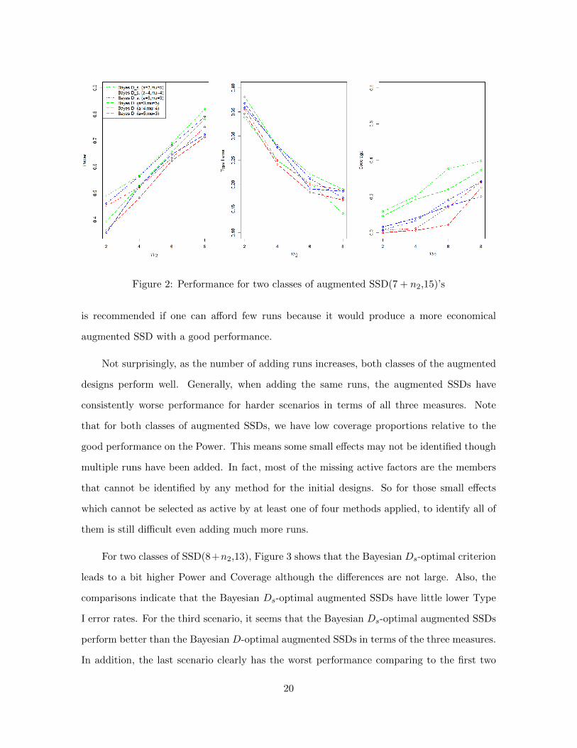
Figure 2: Performance for two classes of augmented SSD(7 + n2,15)’s
is recommended if one can afford few runs because it would produce a more economical
augmented SSD with a good performance.
Not surprisingly, as the number of adding runs increases, both classes of the augmented
designs perform well. Generally, when adding the same runs, the augmented SSDs have
consistently worse performance for harder scenarios in terms of all three measures. Note
that for both classes of augmented SSDs, we have low coverage proportions relative to the
good performance on the Power. This means some small effects may not be identified though
multiple runs have been added. In fact, most of the missing active factors are the members
that cannot be identified by any method for the initial designs. So for those small effects
which cannot be selected as active by at least one of four methods applied, to identify all of
them is still difficult even adding much more runs.
For two classes of SSD(8+n2,13), Figure 3 shows that the Bayesian Ds-optimal criterion
leads to a bit higher Power and Coverage although the differences are not large. Also, the
comparisons indicate that the Bayesian Ds-optimal augmented SSDs have little lower Type
I error rates. For the third scenario, it seems that the Bayesian Ds-optimal augmented SSDs
perform better than the Bayesian D-optimal augmented SSDs in terms of the three measures.
In addition, the last scenario clearly has the worst performance comparing to the first two
20
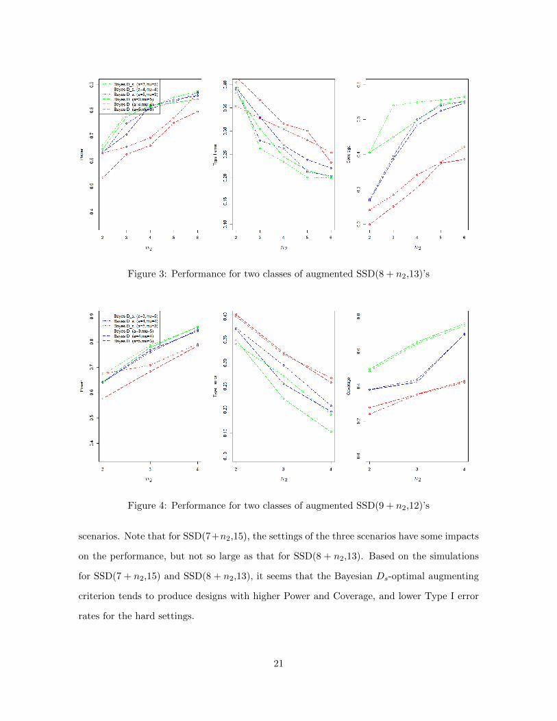
Figure 3: Performance for two classes of augmented SSD(8 + n2,13)’s
Figure 4: Performance for two classes of augmented SSD(9 + n2,12)’s
scenarios. Note that for SSD(7+n2,15), the settings of the three scenarios have some impacts
on the performance, but not so large as that for SSD(8 + n2,13). Based on the simulations
for SSD(7 + n2,15) and SSD(8 + n2,13), it seems that the Bayesian Ds-optimal augmenting
criterion tends to produce designs with higher Power and Coverage, and lower Type I error
rates for the hard settings.
21

For the SSD(9 + n2,12), two classes of augmented SSDs perform well as expected since
the analysis of initial design can present a good classification for the factors, that is about
50% active factors are specified to the primary group and only about 10% active factors are
incorrectly classified into the potential group. Here, the Bayesian Ds-optimal augmented
SSDs do not outperform the Bayesian D-optimal augmented SSDs any more, i.e., two classes
of augmentation methods present similar results in terms of the three evaluation measures.
Through the above simulations, we know that for the initial SSDs with high factor-to-
run ratios, the identification results from various methods are different. When adding fewer
runs are considered, employing the Bayesian Ds-optimal augmented design would be a better
choice. Even the factor-to-run ratio is not very high, if there are great differences in the
results of various methods for the initial SSDs, this performance suggests us that the number
of active factors may be a litter large or there are some small effects, the Bayesian Ds-optimal
augmented design should be the preference too.
Remark 2. When adding follow-up experiments, the practitioners are very concerned about
the practical question, given n1 what will be an ideal value for n2? For traditional SSDs,
Marley and Woods (2010) concluded that the number of all runs should be at least three
times the number of active effects. However, it is not easy to answer this question for the
augmented SSDs since it would involve the objective of experiment, the correlations in the
initial design model, the complexity of the model and so on. In our simulation, we have
considered all the values of n2 ∈ {2, . . . , k + 1 − n1}, though not all results are presented
for SSD(7,15) since Figure 2 can still clearly show the trend of increasing or decreasing for
the three measures. We find that for initial SSDs with moderate factor-to-run ratios, such
as SSD(9,12) and SSD(8,13), adding n2 = k + 1 − n1 runs is enough to present a good
augmented SSD if the model does not include many small active effects. When an SSD with
a high factor-to-run ratio is used in the first stage experiment, difficulty to identify those
relatively small effects would result in an inaccurate factor classification and eventually lead
to a bad result, though the result is somewhat meaningful. In general, the purpose of using
an SSD is just to find the important factors.
22

5 Concluding remarks
SSDs are typically employed to screen a few factors from many candidates and they
have great potential to aid in discoveries in a resource-efficient manner. However, screening
experiments often leave some questions unanswered and adding new runs to the original
experiment should allow us to clear up our uncertainty. In this paper, we have presented the
Bayesian Ds-optimality to add runs to existing SSDs by using information from the initial
experiment. The simulation studies in Section 4 indicate that the augmentation strategy
performs well, especially when we have a proper prior classification for the factors, most of
the active factors and the mean shift can be identified with adding a few runs. Even for those
challenging settings, the factor classification is not so accurate because of the complicated
confounding pattern in the initial design, the analysis results of the final augmented SSDs
are still pretty good, and the Bayesian Ds-optimal augmenting criterion tends to produce
designs with higher Power and Coverage, and lower Type I error rates than the Bayesian
D-optimal augmenting criterion.
Ruggoo and Vandebroek (2004) pointed out the Bayesian D-D optimal designs coming
from two-stage procedures perform more robust and better in comparison to its unique stage
competitors, the classical one-stage D-optimal and the one-stage Bayesian D-optimal designs.
For an augmented SSD, since the added design is generated from the Bayesian Ds(or D)-
optimal procedure that incorporates the improved model knowledge from the first stage and
the experts’ advice, we may expect such an augmented SSD would be superior in performance
to the classical one stage SSDs in some situations and this is also our future work.
There are still some limitations of our simulation studies, more variable selection methods
and designs should be considered, it is possible that classification results from much more
analysis strategies may be more accurate, and then improve the efficiency of the Bayesian
Ds-optimal augmented SSDs in identifying active factors.
In the literature, most of the SSDs are for main effects only models. However, studies
are needed to construct SSDs for the estimation of factor interactions.
23

Acknowledgments
This work was supported by the National Natural Science Foundation of China (Grant
Nos. 11771220, 11431006, and 11601244), Tianjin Development Program for Innovation and
Entrepreneurship, Tianjin “131” Talents Program, and Project 61331903. The authors thank
the Executive-Editor, an Associate-Editor and two referees for their valuable comments.
References
Abraham, B., Chipman, H. and Vijayan, K. (1999). Some risks in the construction and analysis of
supersaturated designs. Technometrics 41, 135–141.
Atkinson, A. C. and Donev, A. N. (1992). Optimum Experimental Designs. Oxford Science Publica-
tions, Oxford.
Beattie, S. D., Fong, D. K. H. and Lin, D. K. J. (2002). A two-stage Bayesian model selection strategy
for supersaturated designs. Technometrics 44, 55–63.
Booth, K. H. V. and Cox, D. R. (1962). Some systematic supersaturated designs. Technometrics 4,
489–495.
Box, G. E. P. (1959). Discusssion on “Random balance experimentation” by F. E. Satterthwaite.
Technometrics 1, 174–180.
Box, G. E. P., Meyer, R. D. (1986). Ananalysis for unreplicated fractional factorials.Technometrics
28, 11–18.
Candes, E. and Tao, T. (2007). The Dantzig selector: statistical estimation when p is much larger
than n n (with discussion). The Annals of Statistics 35, 2313–2351.
Casey, M., Gennings, C., Carter, W. H. J., Moser, V. C. and Simmons, J. E. (2005). Ds-optimal designs
for studying combinations of chemicals using multiple fixed-ratio ray experiments. Environmetrics
16, 129–147.
Chen, R. B., Chu, C. H., Lai, T. Y. and Wu, Y. N. (2011). Stochastic matching pursuit for Bayesian
variable selection. Statistics and Computing 21, 247–259.
Chen, R. B., Weng, J. Z. and Chu, C. H. (2013). Screening procedure for supersaturated designs using
a Bayesian variable selection method. Quality and Reliability Engineering International 29, 89–101.
24

Daniel, C. (1959). Use of half-normal plots in interpreting factorial two-level experiments. Techno-
metrics 1, 311–341.
DuMouchel, W. and Jones, B. (1994). A simple bayesian modification of D-optimal designs to reduce
dependence on an assumed model. Technometrics 36, 37–47.
Fan, J. (1997). Comments on “Wavelets in statistics: a review” by A. Antoniadis. Journal of the
Italian Statistical Society 6, 131–138.
Fan, J. and Li, R. (2001). Variable selection via nonconcave penalized likelihood and its oracle
properties. Journal of the American Statistical Association 96, 1348–1360.
Georgiou, S. D. (2014). Supersaturated designs: a review of their construction and analysis. Journal
of Statistical Planning and Inference 144, 92–109.
Goos, P. and Jones, B. (2011). Optimal design of experiments: a case study approach. John Wiley
and Sons, New York.
Gupta, V. K., Chatterjee, K., Das, A. and Kole, B. (2012). Addition of runs to an s-level supersatu-
rated design. Journal of Statistical Planning and Inference 142, 2402–2408.
Gupta, V. K., Singh, P., Kole, B. and Parsad, R. (2010). Addition of runs to a two-level supersaturated
design. Journal of Statistical Planning and Inference 140, 2531–2535.
Gutman, A. J., White, E. D., Lin, D. K. J. and Hill, R. R. (2014). Augmenting supersaturated designs
with Bayesian D-optimality. Computational Statistics and Data Analysis 71, 1147–1158.
Huang, H. Z., Yang, J. Y. and Liu, M. Q. (2014). Functionally induced priors for componentwise Gibbs
sampler in the analysis of supersaturated designs. Computational Statistics and Data Analysis 72,
1–12.
Jones, B., Lin, D. K. J. and Nachtsheim, C. J. (2008). Bayesian D-optimal supersaturated designs.
Journal of Statistical Planning and Inference 138, 86–92.
Kiefer, J. and Wolfowitz, J. (1961). Optimum designs in regression problems. Annals of Mathematical
Statistics 32, 298–325.
Li, R. and Lin, D. K. J. (2002). Data analysis in supersaturated designs. Statistics and Probability
Letters 59, 135–144.
Lin, D. K. J. (1993). A new class of supersaturated designs. Technometrics 35, 28–31.
Lin, D. K. J. (1995). Generating systematic supersaturated designs. Technometrics 37, 213–225.
25

Marley, C. J. and Woods, D. C. (2010). A comparison of design and model selection methods for
supersaturated experiments. Computational Statistics and Data Analysis 54, 3158–3167.
Nguyen, N. (1996). An alogrithmic approach to constructing supersaturated designs. Technometrics
38, 69–73.
Phoa, F. K. H., Pan, Y. H. and Xu, H. (2009). Analysis of supersaturated designs via the Dantzig
selector. Journal of Statistical Planning and Inference 139, 2362–2372.
Qin, H., Chatterjee, K. and Ghosh, S. (2015). Extended mixed-level supersaturated designs. Journal
of Statistical Planning and Inference 157, 100–107.
Ruggoo, A. and Vandebroek, M. (2004). Bayesian sequential D-D optimal model-robust designs.
Computational Statistics and Data Analysis 47, 655–673.
Salawu, I. S., Adeleke, B. L. and Oyeyemi, G. M. (2015). Review of classical methods in supersaturated
designs (SSD) for factor screening. Mathematical Theory and Modeling 5, 38–44.
Suen, C. and Das, A. (2010). E(s2)-optimal supersaturated designs with odd number of runs. Journal
of Statistical Planning and Inference 140, 1398–1409.
Sun, F. S., Lin, D. K. J. and Liu, M. Q. (2011). On construction of optimal mixed-level supersaturated
designs. Annals of Statistics 39, 1310–1333.
Tibshirani, R. J. (1996). Regression shrinkage and selection via the lasso. Journal of the Royal
Statistical Society: Series B (Statistical Methodology) 58, 267–288.
Westfall, P. H., Young, S. S. and Lin, D. K. J. (1998). Forward selection error control in the analysis
of supersaturated designs. Statistica Sinica 8, 101–117.
Wu, C. F. J. (1993). Construction of supersaturated designs through partially aliased interactions.
Biometrika 80, 661–669.
Yin, Y. H., Zhang, Q. Z. and Liu, M. Q. (2013). A two-stage variable selection strategy for supersat-
urated designs with multiple responses. Frontiers of Mathematics in China 8, 717–730.
Zhang, Q. Z., Zhang, R. C. and Liu, M. Q. (2007). A method for screening active effects in supersat-
urated designs. Journal of Statistical Planning and Inference 137, 2068–2079.
26