A mathematical framework for Dirac’s calculus

Yves Peraire

Abstract.

The observation and the discussion of the physical reality

of phenomena, leads to bring out concepts which have to

be described in a non ambiguous mathematical language.

Concerning Dirac’s calculus we shall introduce, besides the

usual definitions for the concepts of point, number, function

etc ... , additional concepts for the physical point, the

physical equalities, physical infinities and infinitesimals ...

etc ... In particular we introduce a new equality =D , called

Dirac-equality, which differs as well from the classical equality

as from the weak equalities introduced in various theories of

generalized functions. All these definitions are based on a

definition in the language of Relative Set Theory, see [15],

of the metaconcepts of improperness used by P.A.M. Dirac

in [Di], when he claimed ” Strictly of course, δ(x) is not a

proper function of x, ... , ... δ′(x), δ′′(x).... are even more

discontinuous and less proper than δ(x) itself ”. We defined

this way a concept of observed derivative which extends the

usual one to a large class of discontinuous possibly non-

standard functions. All the multiplications of improper or

very improper functions, including the delta-functions and

their observed derivatives, are obviously allowed. Now the

problem of the multiplication is replaced by another one:

under which conditions is the Dirac-equality of two functions

preserved by a multiplication term by term?

1 Basic language and definitions.

We will indicate first how to define the basic vocabulary in order todevelop consistently a discourse similar to that of physicists. Moreprecisely, we want to introduce the words improper, very improper etc.... and elements of vocabulary which play the same role in reasoningthat the constants dx, dy, etc ... and which generalize them by specifyingdegrees in infinitesimality . All this can be defined precisely in thelanguage of Relative Set Theory, RST. This language is built on twobinary predicates : The usual predicate � · ∈ · � and a newpredicate denoted � · SR · �.

1

2

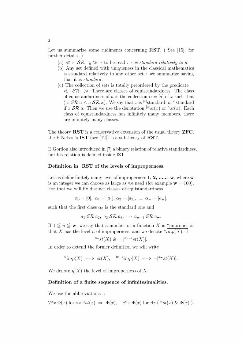
Let us summarize some rudiments concerning RST. ( See [15], forfurther details. )

(a) � x SR y � is to be read : x is standard relatively to y.(b) Any set defined with uniqueness in the classical mathematics

is standard relatively to any other set : we summarize sayingthat it is standard .

(c) The collection of sets is totally preordered by the predicate� · SR · �. There are classes of equistandardness. The classof equistandardness of a is the collection α = [a] of x such that( x SR a ∧ a SR x). We say that x is [a]standard, or αstandardif x SR a. Then we use the denotation [a]st(x) or αst(x). Eachclass of equistandardness has infinitely many members, thereare infinitely many classes.

The theory RST is a conservative extension of the usual theory ZFC,the E.Nelson’s IST (see [12]) is a subtheory of RST.

E.Gordon also introduced in [7] a binary relation of relative standardness,but his relation is defined inside IST.

Definition in RST of the levels of improperness.

Let us define finitely many level of improperness 1, 2, ...... w, wherewis an integer we can choose as large as we need (for example w = 100).For that we will fix distinct classes of equistandardness

α0 = [0], α1 = [a1], α2 = [a2], .... αw= [a

w],

such that the first class α0 is the standard one and

a1 SR a2, a2 SR a3, · · · aw−1 SR a

w.

If 1 5 n 5 w, we say that a number or a function X is nimproper orthat X has the level n of improperness, and we denote nimp(X), if

αnst(X) & ¬ [αn−1st(X)].

In order to extend the former definition we will write

0imp(X) ⇐⇒ st(X), w+1imp(X) ⇐⇒ ¬[awst(X)].

We denote η(X) the level of improperness of X.

Definition of a finite sequence of infinitesimalities.

We use the abbreviations :

∀αx Φ(x) for ∀x αst(x) ⇒ Φ(x), ∃αx Φ(x) for ∃x ( αst(x) & Φ(x) ).

3

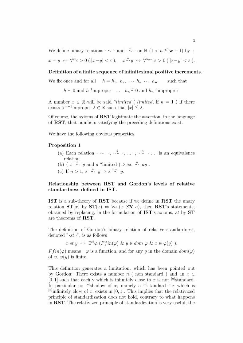
We define binary relations · ∼ · and · n∼ · on R (1 < n 5 w + 1) by :

x ∼ y ⇔ ∀stε > 0 ( |x−y| < ε ), xn∼ y ⇔ ∀αn−1ε > 0 ( |x−y| < ε ).

Definition of a finite sequence of infinitesimal positive increments.

We fix once and for all h = h1, h2, · · · hn · · · hw

such that

h ∼ 0 and h 1improper ... hnn∼ 0 and hn

nimproprer.

A number x ∈ R will be said nlimited ( limited, if n = 1 ) if thereexists a n−1improper λ ∈ R such that |x| 5 λ.

Of course, the axioms of RST legitimate the assertion, in the languageof RST, that numbers satisfying the preceding definitions exist.

We have the following obvious properties.

Proposition 1

(a) Each relation · ∼ ·, · 2∼ ·, ... , · n∼ · ... is an equivalencerelation.

(b) ( xn∼ y and a nlimited )⇒ ax

n∼ ay .

(c) If n > 1, xn∼ y ⇒ x

n−1∼ y.

Relationship between RST and Gordon’s levels of relativestandardness defined in IST.

IST is a sub-theory of RST because if we define in RST the unaryrelation ST(x) by ST(x) ⇔ ∀a (x SR a), then RST’s statements,obtained by replacing, in the formulation of IST’s axioms, st by STare theorems of RST.

The definition of Gordon’s binary relation of relative standardness,denoted ”·st ·”, is as follows

x st y ⇔ ∃stϕ (Ffin(ϕ) & y ∈ dom ϕ & x ∈ ϕ(y) ).

Ffin(ϕ) means : ϕ is a function, and for any y in the domain dom(ϕ)of ϕ, ϕ(y) is finite.

This definition generates a limitation, which has been pointed outby Gordon: There exists a number n ( non standard ) and an x ∈[0, 1] such that each y which is infinitely close to x is not [n]standard.In particular no [n]shadow of x, namely a [n]standard [n]x which is[n]infinitely close of x, exists in [0, 1]. This implies that the relativizedprinciple of standardization does not hold, contrary to what happensin RST. The relativized principle of standardization is very useful, the

4

general principles of transfer idealization and choice we have proved in[16] are linked to the existence of such a possibility of standardization.Now a lot of applications can be treated with Gordon’s predicate.

2 Derivations of classically nonderivable functions

We need first to develop the concept of point. Of course, none of thesedefinitions completely captures the intuitive notion.

2.1 - Various conceptual symbolical patterns for the physicalpoint.Let a be a point and n a level of improperness such that η(a) 5 n.

We put ]a[n=]a−hn, a+hn[. If n = η(a) we use the simplified notations]a[ for ]a[n.

If a is a number and n a level of improperness, which have no relationa priori with η(a), we put o a o n = {x ∈ R : x

n∼ a} and we use thesimplified notation o a o if n = 0.

Remarks.

(1) The symbol o ao n represents a collection which is not a “trueset” in the relative set theory.

(2) In RST, it is not possible to define uniformly the open point]a[ for any a of R by means of a function h : R −→ R whichassociates to any a an infinitesimal strictly less standard thana itself. The reason is that if such an h existed then an elementa ∈ R would exist such that ( h SR a ) because, if a SR hfor any a in R, R would be finite (see [15], Theorem 2) .Then the axiom of transfer would give h(a) SR a and thisis contradictory.

If x ∈ R we shall use the terms :

”Point” to indicate the number x,”open point” to indicate ]x[,”analysed point”to name ox o .

2.2 - The collection R.

The set R below is our basic space of functions. This set could seemvery particular. In reality the possibility for a function u ∈ R tobe improper or very improper makes it very general: In particular, Rcontains exact representatives for any standard or improper distribution.... and more ...

5

Its description requires the next definition.

Definition 1. A subset F of R is said Locally standard-finite if, forany limited x and y, [x, y] ∩ F is finite and its cardinality is standard.

The axioms of RST enable to prove that if F is a locally standard-finite subset of R then a standard subset oF of R exists such that, forany limited x, y ∈ R :

(a) oF ∩ [x, y] is a standard finite set,(b) for any t ∈ F ∩ [x, y] there exists a standard element ot ∈ oF ,

called the shadow of t, such that t ∼ ot.

The set oF is called the shadow of F .

Definition 2. We say that a function f R −→ R is regular if

(a) it have a level of improperness among the levels {1, 2, ,w}fixed above,

(b) f is C∞ at any point except the points of a locally standard-finite possibly empty set F (f),

(c) f has all order left and right derivatives at any point of F (f).

We denote R the collection of regular functions. In this paper, iff, g ∈ R we put f = g if there exits a finite set F (possibly nonstandard) such that for any t ∈ R \ F, f(t) = g(t).

Basic examples.

In these examples, for any subset A of R, χA denotes the characteristicfunction of A.

1. The Heaviside function Ha at the point a defined by Ha =χ[a,+∞[ is regular and F (Ha) = {a}.

2. If we simplify H0 in H, f = H ◦ sin is regular and F (f) = π ·Z3. Let a ∈ R with the level η(a) of improperness, 0 5 η(a) < w.

We define the principal evaluation δa of the Dirac-function atthe point a by

δa =1

2hη(a)

χ]a[. We will simplify δ0 in δ.

δa is η(a)+1improper, regular and F (δa) = {a− hη(a), a+ h−η(a)}.4. We shall need also ”hyperevaluations” of the Dirac-function.

If 0 5 η(a) < n 5 w, we putn

δa =1hnχ]a[n .

This implies that1

δa = δa. We shall use the simpler notations

δa rather thanη(a)+1

δa , and δ for2

δ.

6

5. The functions P and Z

P (x) = 1− χ]0[, Z(x) = χ]−h,0[ − χ]0,h[.

6. Principal evaluation of the function1

x.

1=x=

P (x)

x− 1

hZ(x)

Principal evaluation of the logarithm

Ln(x) = P ln(x)

Other evaluations in R of the Dirac-function and1

xwill be considered

elsewhere.

1=x

1

h__

1

h__--h h

1__2h

1

P(x)

-h h

1

Z(x)

-h h

Figure 1. Graphical Representations of some improper evaluations

δ(x)

Definition 3. Let f ∈ R be a n−1improper function, with 1 5 n 5 w.We call observed derivative of f , the function f ]′[ defined by

f ]′[(x) =f(x+ hn)− f(x− hn)

2hn

.

For any finite integer k such that n+ k 5 w, we put

f ]′′[ = (f ]′[)]′[, · · · , f ]k[ = (f ]k−1[)]

′[.

7

We also define in a natural way, for any n−1improper function f ∈ R,and any k such that 0 5 n < k 5 w, the khyper-observed derivative

f ]′[k(x) =f(x+ hk)− f(x− hk)

2hk

.

It will be noticed that the index k in f ]′[k(x) indicates the level ofimproperness of the hyper-observed derivative. It would be possibleto also define concepts of hyper-observed second derivative, hyper-observed third derivative etc.....

Examples :

(1) For any standard a ∈ R, Ha is standard, 0improper, so

H ]′[a =

1

2h[ Ha+h−Ha−h ] = δa, H

]′[2a =

1

2h2

[ Ha+h2−Ha−h2 ] =

δa,(2) δa is 1improper hence

δ]′[a =

1

2h2

[ δa+h2−δa−h2 ], δ]′[3a =

1

2h3

[ δa+h3−δa−h3 ].

δ]′[a is 2improper, δ

]′[3a is 3improper.

Figure 2 below represents δ]′[. It is only a synoptic representation : we

consider that we are really unable to see precisely inside the point.

]-h[

]h[

(1/2h) . (1/2h2)

- (1/2h) . (1/2h2)

Figure 2. The function δ]′[(x)

If we denote, for any function f ∈ R with the level n−1 of improperness,

f+(x) = f(x+ hn) and f−(x) = f(x− hn).

then the observed derivatives have the obvious following properties.

8

For any f, g ∈ R with the same level of improperness

(f + g)]′[ = f ]′[ + g]

′[, (1)

(f g)]′[ = f ]′[ g+ + f− g]

′[. (2)

These formulae are false if f and g don’t have the same degree ofimproperness, for example

(H +Hh)]′[ = δ + δh,

H ]′[ +H]′[h = δ + δh.

The second formula is not the exact formula of Leibnitz,‘

(f g)]′[ = f ]′[ g + f g]

′[.

However, physicists sometimes freely use formula (1), the formula ofLeibnitz as well as the formula of integration by parts even in thepresence of jumps, and this does not seems to lead to any concretephysical contradiction.

The introduction, besides the concepts above, for points functions andderivatives, of a concept of equality adapted to the physicist’s discourse,will lighten the mystery.

2-4 Dirac-equalities.

Dirac considers that any improper function whose value is zero outsideof the origin and such that the integral is egal to 1, is identical to delta.Starting from this idea, we will define a relation between elements of Rwhich, according to our opinion, is more significant than the classicalweak equality of distributions. Its definition uses the below definitenotion of reiterated primitives.

If f ∈ R, we denote

∫ x

1 a

f(s) ds =

∫ x

a

f(s) ds,

∫ x

2 a

f(s) ds =

∫ x

a

dt

∫ t

a

f(s) ds,

. . . ,

∫ x

an+1

f(s) ds =

∫ x

a

dt

∫ t

1 a

f(s) ds . . .

The next proposition gives useful values and infinitesimal approximationsof some reiterated primitives. Let us denote y << a << x if y < a < x,x /∈ o a o and y /∈ o a o . Then we can state.

9

Proposition 1. for any y, a, x such that y << a << x, for anystandard k ∈ N

?, for any n > η(a)

(1)

∫ x

k y

Ha =(x− a)k

k!, (2)

∫ x

k y

n

δan∼ (x− a)k−1

(k − 1)!,

(3)

∫ x

k y

(n

δa)2 n∼ (x− a)k−1

2hn (k − 1)!, (4)

∫ x

y

(t−a)n

δa(t) dt = 0,

(5)

∫ x

2 y

(t−a)n

δa(t) dt = −h2n

3, if k > 1 (6)

∫ x

k y

(n

δa)]′[ n∼ (x− a)k−2

(k − 2)!.

Proof. These results are obtained through elementary calculations. Theproof of (1) is obvious. Let us prove (2). We will remark first that

n

δa =1

2hn

[Ha−hn−Ha+hn

].

An application of (1) gives∫ x

k y

n

δa =(x− (a− hn))

k − (x− (a+ hn))k

2hnk!=

(x− (a− hn))k−1+ (x− (a− hn))

k−2(x− (a+ hn)) + · · ·+ (x− (a+ hn))k−1

k!.

If we remark that each of the k terms between the brackets is ninfinitelyclose to (x − a)k−1, we obtain (2). The proofs of (3), (4) and (5) arelet to the reader. In order to prove (6) let us remark first that

(n

δa)]′[ =

1

2hn

[n+1

δ a−hn−

n+1

δ a+hn

].

The sequel of the proof makes use of (2) and the binomial formula.

We generalize the definition of analyzed points by writing

o +∞o = {x ∈ R : x ∼ +∞}, o −∞ o = {x ∈ R : x ∼ −∞}.For any locally standard-finite set F , we denote

oF o =⋃

x∈F∪{−∞,+∞}

ox o .

For any set F we put]F[n=

⋃

x∈F

]x− hn, x+ hn[.

10

Definition 4. Let f and g be elements of R and let n be a standardinteger. We say that f is Dirac-equal to g without integration anddenote f =D

0 g, or more precisely f =D0 g (F ), if there exists a locally

standard-finite set F such that for any standard order of derivation k(in the classical sense) for any x ∈ R, x /∈ oF o ⇒ f (k)(x) ∼ g(k)(x).

We say that f is Dirac-equal to g up to n integration and denote itf =D

n g, or more precisely f =Dn g (F ), if a locally standard-finite set

F exists such that for any a, b ∈ R,

a, b /∈ oF o ⇒∫ b

k a

f(x) dx ∼∫ b

k a

g(x) dx for any k ∈ { 1, ..., n }.

We say that f is Dirac-equal to g, and denote f =D g, if for anystandard n ∈ N, f =D

n g.

Theorem. For any standard integer n

(a) For any f , g, h in R : f =Dn g and g =D

n h ⇒ f =Dn h

(b) For any f , f1, g, g1 in R :

( f =Dn f1 and g =D

n g1 ) ⇒ f + g =Dn f1 + g1

Proof. The proof is a simple check.

A general result similar to (b) relative to the usual product of functionsdoes not exists.

Counterexamples :

1 - Hδ =D 1

2δ but H(Hδ) = Hδ =D 1

2δ 6=D 1

4δ =D H (

1

2δ).

2 - If f is constant, f =1

2h, g = H−h−Hh then g =D 0 but fg = δ 6=D 0.

However, we shall see useful particular cases in section 3, theorem 8and 9.

The next proposition states some useful relations.

11

Proposition 2. Let a ∈ R be such that η(a) 5 w :

(1) If η(a) < n 5 m 5 w, then for any λ ∈ R such that η(λ) 5 n−1,

λn

δa =D λm

δ a. In particular, δa =D δa.

(2) Ha δa =D1

2δa, (3) δaδa =

D δ2a, (4)1

xδh =D

1 2δ2 but1

xδh 6=D 2δ2.

(5) δ]′[a =D

0 0, (6)

∫ x

−∞

δ]′[a =D δa, (7) δ2a 6=D δ2a, (8)

1=xδ =D− 1

2δ]

′[,

(9) δa δa+ =D1

1

2δ2a but δaδa+ 6=D 1

2δ2a, (10)

1

2hZ =D 0, (11)

1

2hZ ]′[ =D 0,

(12)( 1

2h

)2Z =D

1

4δ]′[

, (13) Hδ2 =D1

1

2δ2 but Hδ2 6=D 1

2δ2,

(14)1

2h( δ − δh ) =

D1

2δ]

′[, (15)1=x

δ]′[ =D − 4 δ2δ − 1

2δ]”[ =D

1 −4 δ3 − 1

2δ]”[,

(16)( 1=x

)]′[δ =D 4 δ2 δ =D

1 4 δ3.

Proof. (1) The functions λn

δa =D λn

δa and λn

δa =D λm

δ a have the value0 outside o a o . It remains to be shown that the reiterated integrals areinfinitesimally close one to the other. In order to prove it let us fix xand y such that x /∈ o a o and y /∈ o a o . From the former propositionwe get

∫ x

k y

n

δan∼ (x− a)k−1

(k − 1)!

m∼∫ x

k y

m

δ a hence

∫ x

k y

n

δan∼

∫ x

k y

m

δ a.

Multiplying term by term by the nstandard number λ we obtain

λ

∫ x

k y

n

δa =

∫ x

k y

λn

δan∼

∫ x

k y

λm

δ a = λ

∫ x

k y

m

δ a.

(2) and (3) are obvious. Let us prove (4). let us fix x and y such that

x /∈ o a o , y /∈ o a o and y < a < x. Let us denote ϕ(t) =

∫ t

y

1

sδh(s) ds.

1

sδh(s) = 0 if s /∈ [h] and, if s ∈ [h]

1

2h2(h+ h2)5

1

sδh(s) 5

1

2h2(h− h2).

Taking the integral we obtain

1

h+ h2

5 ϕ(x) =

∫

[h]

1

sδh(s) ds 5

1

h− h2

.

As1

h+ h2

2∼ 1

h

2∼ 1

h− h2

and

∫ x

y

δ2 =1

2h, we obtain

1

xδh =D

1 2δ2.

This implies

12

∫ x

2 y

1

tδh(t) dt =

∫ x

y

ϕ(t) dt 5x− (h− h2)

h− h2

.

Now, it follows from x /∈ o 0 o and h22∼ 0 that

x− (h− h2)

h− h2

2∼ x

h− 1.

On the other hand,

∫ x

2 y

δ2 ∼ x

2h. Hence

∫ x

2 y

1

tδh(t) dt 6∼

∫ x

2 y

2δ2(t) dt

and this implies that 1xδn 6=D 2δ2.

We let to the reader the proofs of (5), (6)and (7). Let us prove (8).

We deduce from the formula1=xδ =

1

2h2[−H−h + 2H −Hh] that

∫ x

k y

1=xδ =

−(x+ h)k + 2xk − (x− h)k

2h2k!∼ −1

2

xk−2

(k − 2)!∼

∫ x

k y

−1

2δ]

′[.

Let us prove (9) now. We have δδh =D0

12δ2 because both δδh and 1

2δ2

have the value zero outside of o 0 o . Let now x and y be elements ofR \ o 0 o . If y < 0 < x then an easy calculation gives

∫ x

n y

δδh =(x− (h− h)n − (x− h)n

4hh2n!,

∫ x

n y

1

2δ2 =

(x+ h)n − (x− h)n

4h2n!.

So we obtain :

with n = 1 :

∫ x

1 y

δδh =

∫ x

1 y

1

2δ2 =

1

h,

with n = 2 :

∫ x

2 y

δδh =12hx− 1

4,

∫ x

2 y

1

2δ2 =

x

8h. Hence

δδh =D1

1

2δ2, but δδh 6=D 1

2δ2 because δδh 6=D

2

1

2δ2.

the formulas (10) to (16) are left to the reader.

Let us consider now the following functions, which usually play the roleof Dirac-functions in physics.

δ1(x) =1

2he−

|x|h , δ2(x) =

1

π

h

x2 + h2, δ3(x) =

1

h√π

e−x2

h2 , δ4(x) =sin(x

h)

πx.

Then we have

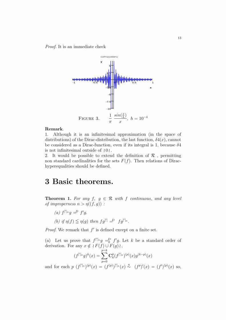
Proposition 3. δ1 =D δ2 =D δ3 =D δ but δ4 6=D δ .If a ∼ ±∞ and ξa =

12h

(Ha− −Ha+) then ξa =D 0 .

13

Proof. It is an immediate check

10.50-0.5-1

5

2.5

0

-2.5

-5

-7.5

-10

x

y

x

y

1/x/PI*sin(10000*x)

Figure 3.1

π

sin(xh)

x, h = 10−4

Remark.1. Although it is an infinitesimal approximation (in the space ofdistributions) of the Dirac-distribution, the last function, δ4(x), cannotbe considered as a Dirac-function, even if its integral is 1, because δ4is not infinitesimal outside of o 0 o .2. It would be possible to extend the definition of R , permittingnon standard cardinalities for the sets F (f). Then relations of Dirac-hyperequalities should be defined.

3 Basic theorems.

Theorem 1. For any f, g ∈ R with f continuous, and any levelof improperness n > η((f, g)) :

(a) f ]′[ng =D f ′g.

(b) if η(f) 5 η(g) then fg]′[ =D fg]

′[n .

Proof. We remark that f ′ is defined except on a finite set.

(a) Let us prove that f ]′[ng =D0 f ′g. Let k be a standard order of

derivation. For any x /∈ oF (f) ∪ F (g) o ,

(f ]′[ng)k(x) =

p=k∑

p=0

Cpk(f

]′[n)(p)(x)g(k−p)(x)

and for each p (f ]′[n)(p)(x) = (f (p))]′[n(x)

n∼ (f p)′(x) = (f ′)(p)(x) so,

14

each g(k−p)(x) being nlimited, we have

(f ]′[ng)k(x)n∼

p=k∑

p=0

Cpk(f

′)(p)(x)g(k−p)(x) = (f ′g)(k)(x).

This prove f ]′[g =D0 f ′g. Let us compare the reiterated integrals.

For any limited x, y,∫ y

x

f ]′[n(t)g(t) dt =

∫ y

x

f(x+ hn)− f(x− hn)

2hn

g(t) dt.

If x does not belong to any ]a[n with a ∈ F (f) then

f(x+ hn)− f(x− hn)

2hn

= f ′(x+ θhn) with θ ∈]− 1, 1[.

Now, by the definition of R, f ′ is uniformly continuous over eachinterval of continuity of f , so

f ′(x+ θhn)n∼ f ′(x), f ′(x+ θhn)g(x)

n∼ f ′(x)g(x)

because g is nlimited, and

∫ y′

x′

f ′g ∼∫ y′

x′

f ]′[ng whatever x′, y′ such

that [x′, y′] ⊂ ([x, y] \ ]F (f)[n.

If a ∈ F (f), then f ′g and f ]′[ng are both nlimited on ]a[n so the integrals∫ y”

x”

f ′g and

∫ y”

x”

f ]′[ng are infinitesimals for any x”, y” ∈]a[n, a ∈ F (f),

because |y”− x”| is ninfinitesimal.

We conclude that

∫ y

x

f ′g ∼∫ y

x

f ]′[ng. Computing the iterated primitives

up to a standard rank k, we get

∫ y

xk

f ′g ∼∫ y

xk

f ]′[ng.

Hence f ′g =D f ]′[ng.

(b) Let us expand g ∈ R in the form g = u +∑

ai∈G

αiHai , with locally

standard-finite G and continuous u ∈ R. An easy proof, making useof the axiom of transfer, see [15], shows that η(u) 5 η(g) < n and forany i ∈ G, η(ai) 5 η(g) < n, η(αi) 5 η(g) < n.

As G is locally standard-finite then for any limited x and y the integrals∫ x

k y

fg]′[ and

∫ x

k y

fg]′[n are respectively equal to

∫ x

k y

fu]′[η(g)+1 +∑

ai∈Gx,y

∫ x

k y

f.(αiHai)]′[η(g)+1

15

and

∫ x

k y

fu]′[n +∑

ai∈Gx,y

∫ x

k y

f [αiHai ]]′[n .

This sum being standard-finite, we only have to prove

fu]′[η(g)+1 =D fu]′[n and f.(αiHai)]′[η(g)+1 =D f.(αiHai)

]′[n .

The first relation is an application of (a). Item (a) applies because

n = η(g) + 1 > η(g) ≥ η(u), and η(g) = η(f) ⇒ η(g) + 1 > η(u, f).

The last inequality is a consequence of the axiom of transfer.

The second Dirac-equality follows from

f.(αiHai)]′[η(g)+1 =D f(ai)αi

η(g)+1

δ ai =D f(ai)αi

n

δai =D f(αiHai)

]′[n ,

the verification of which is easy.

In order to prove the necessity of the hypothesis, we have to producecounterexamples.

Counterexamples.

(1) With f = H and g = H we have, f ′ = 0 ⇒ f ′g = 0. f ]′[ = δ,

f ]′[g =D1

2δ. So f ′g 6=D f ]′[g. The missing assumption is the continuity

of f

(2) Let be f(x) =

0 if x ≤ h2

1

hx− h

2 hif x ∈ [h

2, h

2+ h]

1 if x ≥ h2+ h

and g = H.

Then f is continuous, fH ]′[2 = f δ = 0 and fH ]′[ = fδ =D1

4δ. In this

example the problem comes from the relation η(f) > η(g).

(3) Concerning (b), let f(x) = δ3 and g(x) = x3. An easy computationyields g]

′[(x) = 3x2 + h2, so f(x)g]′[(x) − f(x)g′(x) = h2δ3. Now the

computation of the first integral prove that h2δ3 6=D 0. We shouldobtain the Dirac-equality replacing g]

′[ by g]′[2 .

Corollary. For any f ∈ R and any standard integer n ≥ η(f),

f ]′[ =D f ]′[n and f ]′[ =D f ′ if f is continuous.

16

Theorem 2. For any f ∈ R and y, x /∈ oF (f) o ,∫ x

y

f ]′[(t) dt ∼ f(x)− f(y).

Proof. Any function of R decomposes in a sum of elementary functions.It is enough to prove the theorem for these elementary functions. Theresult is obvious if f is a continuous function. If f = αHa with limited

a then f ]′[ = αn

δa with n = Max{η(α), η(a)}+1 . For any y, x

∫ x

y

f ]′[ =

α if y << a << x,

0 if y, x << a, or y, x >> a

= f(x)− f(y).

Theorem 3. For any f, g ∈ R, whatever their level of improperness :

(f + g)]′[ =D f ]′[ + g]

′[

Proof. Let n = Max{η(f), η(g), η(f + g)} + 1. Then by the definition

of nhyperobserved derivatives we have (f + g)]′[n = f ]′[n + g]

′[n . Now,the corollary above and properties (a), (b) gives,

(f + g)]′[ =D (f + g)]

′[n = f ]′[n + g]′[n =D f ]′[ + d]

′[.

Theorem 4. For any f, g ∈ R, whatever their level of impropernessif n ≥ η((f, g)) + 1 :

(fg)]′[n =D f g]

′[n + g f ]′[n

Proof. It is enough to show it for elementary functions .

If f = αHa and g = βHb.

If a < b.

Then n is strictly larger than η(a), η(b), η(α) and η(β) (Transfer). Sowe have

f ]′[n = αn

δa, g]′[n = β

n

δb, (fg))]′[n = (αβHb)

]′[n = αβn

δb

]a[n∩]b[n= ∅ ⇒{fg]

′[n = αβHa

n

δb = αβn

δb and

f ]′[ng = αβn

δaHb = 0Hence the formula is true.

If a = b

(fg)]′[n = αβ

n

δa, f ]′[ng = g]′[nf = αβHa

n

δa =D αβ

2

n

δa

If f is continuous and g = Ha.

17

Then (fHa)]′[n(x) = f(x− hn)

n

δa(x) + f ]′[n(x)Ha+hn

(x). The facts thatf is continuous and that the jumps of the successive derivatives havea level of improperness strictly less than n allow us to prove, through

an easy calculation that fhn

n

δa =D f

n

δa and f ]′[nHa+hn

=D f ]′[nHa.

The proof is immediate also if both f and g are continuous elementsof R.

Corollary 1 If f and g have the same level of improperness then

(fg)]′[ =D fg]

′[ + gf ]′[.

There is nothing to prove.

If f and g have distinct levels of improperness there are counterexamples.

Counterexamples.

(1) Let f and g be respectively H and Hh.

Then f.g = Hh, (fg)]

′[ = δh, fg]

′[ = Hδh= δ

h. An easy calculation

gives f ]′[g = δHh=D 1

2δ. so (fg)]

′[ 6=D fg]′[ + gf ]′[.

(2) This counterexample aims at proving that, even if f and g aregenerated, starting from the standard elements of R, by observedderivations, then the rule of corollary 1 does not generally apply. Letus take f = H and g = δ]

′[. We obtain directly (H δ]′[)]

′[ = H δ]′′[,

and the Leibniz rule would give (H δ]′[)]

′[ = δδ]′[ +H δ]”[. Now, we can

verify directly that δ δ]′[ 6=D 0, or wait until theorem 6 in order to use

the arguments that δ δ]′[ =D

1

2(δ2)]

′[ 6=D 0 for δ2 6=D 0.

Corollary 2. For any f, g ∈ R, if f is continuous and η(f) 5 η(g)then

(fg)]′[ =D fg]

′[ + f ′g.

Proof (fg)]′[ = (fg)]

′[η(g) = fg]′[η(g)+1 + f ]′[η(g)+1 (Theorem 4). Now

theorem 1 gives f ]′[η(g)+1g =D f ′g. This end the proof.

Example :

Let xq+ = H.xq, q being a standard positive integer. Then for any

standard integer n,

(xq+ δ]n[)]

′[ =D q xq−1+ δ]n[ + xq

+ δ]n+1[.

18

Remark.

Let be f ∈ R with f(t) 6= 0 for all t. Then we can verify the formula

(1

f)]

′[ = − f ]′[

(f−)(f+).

However, (1

f)]

′[ is not generaly Dirac-equal to −f ]′[

f 2. In order to prove

it, let us consider f = 1 + H. We have f ]′[ = δ,1

f= 1 − 1

2H,

1

f 2= 1− 3

4H,

(1

f)]

′[ = −1

2δ, −f ]′[

f 2= −δ (1− 3

4H) =D − 5

8δ.

Now, corollary 1 allows us to write from the equality1

ff = 1,

(1

f)]

′[ f =D − 1

ff ]′[.

The difficulty lies in the illegality of the multiplication by 1fof the two

members of a Dirac-equality.

Demonstrations of theorems 5 and 6 below, derive directly from thedefinition of the relations =D

k and =D.

Theorem 5. For any f, g ∈ R and any standard k ∈ N?,

( f =Dk g (F ) and a /∈ oF o ) ⇒ (x →

∫ x

a

f) =Dk−1 (x →

∫ x

a

g).

Theorem 6 For any f, g ∈ R, and any k ∈ N,

f =Dk g ⇒ f ]′[ =D

k+1 g]′[.

Theorem 7. For any f, ϕ ∈ R, if ϕ is C∞ on R, if ϕ−1(F (f)) andϕ−1(oF (f)) are locally standard-finite then f ◦ϕ ∈ R and for any leveln > η((f, ϕ)) of improperness

(f ◦ ϕ)]′[ =D (f ]′[n ◦ ϕ)× ϕ′.

To avoid complicated denotations, we shall suppose that ϕ is standard.The general result is obtained through a classical shift of the levels ofimproperness.

19

Lemma. If ϕ is continuous on R:

(a) For any limited a ∈ R and any locally standard-finite and

standard F0 ⊂ R, [−a, a]⋂

ϕ−1( oF0 o ) ⊂ oϕ−1(F0) o .

(b) For any locally standard-finite F ⊂ R : oϕ−1(F ) o ⊂oϕ−1(oF ) o .

Proof. Let x ∈ [−a, a]⋂

ϕ−1( oF0 o ) then there exits u0 ∈ F0 suchthat ϕ(x) ∼ u0. From x limited and ϕ standard we deduce that x hasa shadow ox and ϕ(x) is limited. Also u0 is limited. Now from F0

standard and locally standard finite we deduce that u0 is standard.From the continuity of ϕ we get ϕ(x) ∼ ϕ(ox). Hence

ϕ(ox) = u0,ox ∈ ϕ−1(F0), x ∈ oϕ−1(F0) o .

This prove the inclusion of (a). Let us prove (b).If x ∈ oϕ−1(F ) o then there exists a such that x ∼ a and ϕ(a) ∈ F .We have ϕ(oa) = oϕ(a) ∈o F . From x ∼ oa, and oa ∈ ϕ−1(oF ) wederive x ∈ oϕ−1(oF ) o . This ends the proof of (b).

Proof of Theorem 7.

Case where f is continuous.

Let us prove that (f ◦ ϕ)]′[ =D (f ]′[n ◦ ϕ)ϕ′ ( ϕ−1(oF (f)) ).It makes sense because ϕ−1(oF (f)) is locally standard-finite.The function f being in R its derivatives exists on R \ F . Hence,(f ◦ ϕ)(p) exists on ϕ−1(F (f)) at any order p . The function f ◦ ϕ iscontinuous so we have, from the corollary of theorem 1

(f ′ ◦ ϕ)× ϕ′ = (f ◦ ϕ)′ =D (f ◦ ϕ)]′[ ( ϕ−1(F (f)) ).

As oϕ−1(F ) o ⊂ oϕ−1(oF ) o (lemma, (b))

(f ′ ◦ ϕ)× ϕ′ = (f ◦ ϕ)′ =D (f ◦ ϕ)]′[ ( ϕ−1(oF (f)) ).

It remains to prove that

(f ′ ◦ ϕ)× ϕ′ =D (f ]′[n ◦ ϕ)× ϕ′ ( ϕ−1(oF (f)) ).

(a) Proof of : (f ′ ◦ ϕ)× ϕ′ =D0 (f ]′[n ◦ ϕ)× ϕ′ ( ϕ−1(oF (f)) ).

Let be x /∈ oϕ−1(oF (f)) o then , item (b) of lemma, x /∈ oϕ−1(F (f)) o .Consequently ϕ(x) /∈ F (f) and (f ′)(k)(ϕ(x)) ∼ (f ]′[n)(k)(ϕ(x)) for anystandard k. Multiplication by limited products of ϕ(p)(x), member bymember conserve the relation ∼. We remark that (f ]′[n)(p) = (f (p))]

′[n

for any p. We deduce from these facts that for any limited k,

((f ′ ◦ ϕ)(x)ϕ′(x))(k) ∼ ((f ]′[n ◦ ϕ)(x)ϕ′(x))(k).

20

Proof of : ∀standardk ∈ N (f ′◦ϕ)×ϕ′ =Dk (f ]′[n ◦ϕ)×ϕ′ ( ϕ−1(oF (f)) ).

It is enough to prove that for any x /∈ oϕ−1(oF (f)) o and any limited y

∫ y

x

(f ′ ◦ ϕ)(t)× ϕ′(t) dt ∼∫ y

x

(f ]′[n ◦ ϕ)(t)× ϕ′(t) dt

even if y is in oϕ−1(oF (f)) o . We have to consider mainly the caseswhere [x, y] ∩ oϕ−1(oF (f)) o ⊂ o y o n because [x, y] is an union ofstandard finitely many such intervals.

If y /∈ oϕ−1(oF (f)) o n then f ′(s)n∼ f ]′[n(s) for all s ∈ [ϕ(x), ϕ(y)]

so

∫ y

x

(f ′ ◦ ϕ)(t)× ϕ′(t) dt =

∫ ϕ(y)

ϕ(x)

f ′(s) dsn∼

∫ ϕ(y)

ϕ(x)

f ]′[n(s) ds

=

∫ y

x

(f ]′[n ◦ ϕ)(t)× ϕ′(t) dt.

If y ∈ oϕ−1(oF (f)) o n then for any nimproper integer m >1

|y − x| ,

[x, y − 1

m] ⊂ R \ oϕ−1(oF (f)) o n. Such an integer exists because x /∈

oϕ−1(oF (f)) o , ⇒ x � y. This implies that for any any nimproperm ∈ N ,

m >1

|y − x| =⇒∫ y− 1

m

x

(f ′◦ϕ)(t)×ϕ′(t) dtn∼∫ y− 1

m

x

(f ]′[n◦ϕ)(t)×ϕ′(t) dt.

Now a so-called principle of permanence of non standard mathematicsallows us to say that this infinitesimal equivalence remains true forsome ninfinitely large integer m.

Both

∫ y

y− 1m

(f ′ ◦ ϕ)(t) × ϕ′(t) dt and

∫ y

y− 1m

(f ]′[n ◦ ϕ)(t) × ϕ′(t) dt are

ninfinitesimal because the length of the interval [y− 1

m, y] is ninfinitesimal

and the function (f ′ ◦ ϕ)(t) × ϕ′(t) as well as (f ]′[n ◦ ϕ)(t) × ϕ′(t) isnlimited.

Case where f = µ H, and ϕ has only one (isolated) zero a.

Let be n ≥ η((a, ϕ)).

If f is locally increasing or decreasing, let α and β such that ϕ(α) = −hn

and ϕ(β) = hn. Then we have

21

If ϕ is locally increasing

f ◦ ϕ = µ H ◦ ϕ = µ Ha

µ H−hn◦ ϕ = µ Hα

µ Hhn◦ ϕ = µ Hβ

If ϕ is locally decreasing

f ◦ ϕ = µ H ◦ ϕ = µ (1−Ha)

µ H−hn◦ ϕ = µ (1−Hα)

µ Hhn◦ ϕ = µ (1−Hβ)

If ϕ is locally increasing

(f ◦ ϕ)]′[ = (µ Ha)]′[ = µ δa

(f ]′[n ◦ ϕ)× ϕ′ =µ (H−hn

◦ ϕ−Hhn◦ ϕ)× ϕ′

2hn

=µ(Hα −Hβ)

2hn

× ϕ′

Now,1

2hn

µ (Hα −Hβ)×ϕ′ is Dirac-equal to µ, δa for it is zero outside

of o a o , it have a constant sign, and if y << a << x then∫ x

y

1

2hn

µ (Hα −Hβ)× ϕ′) =1

2hn

µ,

∫ β

α

ϕ′ =1

2hn

µ(ϕ(β)− ϕ(α))

= µ1

2hn

· 2hn = µ. Hence: (f ◦ ϕ)]′[ =D (f ]′[n ◦ ϕ)× ϕ′.

The proof is quite similar if ϕ is locally decreasing.

If a is a local extremum then f ◦ ϕ is constant, its value is µ or 0 so(f ◦ϕ)]′[ is 0. So is (f ]′[n ◦ϕ)×ϕ′, because H−hn

◦ ϕ = Hhn◦ ϕ = 1 or 0.

The reader is now able to proceed alone to the more general case.

If η(f) ≥ η(ϕ), the formula of the theorem becomes

(f ◦ ϕ)]′[ =D (f ]′[ ◦ ϕ)ϕ′.

If η(ϕ) > η(f) the formula (f ◦ ϕ)]′[ =D (f ]′[ ◦ ϕ)ϕ′ could be false.

Counterexample.

f = H and ϕ(x) = hx2 give :(f ◦ ϕ)]

′[ = 0 . For any locally standard-finite F ⊂ R, there existsx such that −x, 2x /∈ oF o , −x << 0 << 2x 5 1. (f ]′[ ◦ ϕ)ϕ′(x) =

(H ]′[(hx2))× 2hx = δ(hx2) 2hx 6=D 0, because

∫ 2x

−x

δ(ht2)× 2h t dt =

1

2hh[t2]2x−x

=3x2

2� 0 .

22

Corollary. for any f ∈ R and any derivable standard ϕ such that ϕ′

have isolated zeros then f ◦ ϕ ∈ R and

(f ◦ ϕ)]′[ =D (f ]′[ ◦ ϕ)ϕ′.

Proof. The reason is that under the assumption on ϕ, ϕ−1(F (f)) andϕ−1(oF (f)) are locally standard-finite. Let us prove it. Let [x, y] be astandard compact interval then ϕ([x, y]) is a standard compact intervaltoo so, it contains a finite-standard number of element of F (f).If ϕ−1(F (f)) ∩ [x, y] or ϕ−1(oF (f)) contains non finite-standard manyelements then c ∈ F (f) exists such that card(ϕ−1({c})) is not standard-finite. This implies that the standard set Z = (ϕ′)−1({0})) ∩ [x, y] isinfinite and contradicts the hypothesis that the zero of ϕ′ are isolated.Hence card(ϕ−1(F (f)) ∩ [x, y]) and ϕ−1(oF (f)) are standard-finite.

Examples.

(1) H(x2) = 1 gives H(x2)]′[ = 0. With de denotations of theorem 7

we have F (f) =oF (f) = ϕ−1(oF (f)) = {0} soH(x2)]′[ =D δ(x2)×

x2. Hence δ(x2)× x2 =D 0, which can be obtained also througha direct calculation.

(2) δ(x2)]′[ =D δ]

′[(x2)× x2.

Open problem. What happens if it is only supposed that ϕ ∈ R.Under which conditions is the formula (f ◦ ϕ)]′[ =D (f ]′[ ◦ ϕ)ϕ]′[ true?

The next theorems, 8 and 9, approach the problem of the conservationof the Dirac-equality after a multiplication term by term.

Theorem 8. For any f, g ∈ R and any standard integer n

f =D g ⇒ xn f =D xn g.

Proof. It is enough to prove that f =D g ⇒ x f =D x g, and oneobtains the theorem through an induction. Let us prove inductivelythat the property P (n) : ∀ f, g ∈ R ( f =D

n g ⇒ x f =Dn x g ),

is satisfied for any standard n. P (0) is obvious. The reason is that forany x /∈ oF (f) o ∪ oF (g) o , and any limited order k = 0 of derivation,(xf(x))(k) = xf (k)(x)+kf (k−1)(x). The numbers x and k being limited,the relations f (k)(x) ∼ g(k)(x) and f (k−1)(x) ∼ g(k−1)(x) (if k > 0)involve xf (k)(x) ∼ xg(k)(x) and, if k > 0, kf (k−1)(x) ∼ kg(k−1)(x).Hence (xf(x))(k) ∼ (xg(x))(k).

Let us suppose P (n) for a fixed standard n. Let f, g be elements

of R Let us fix y /∈ oF (f) o ∪ oF (g) o . Let us put F (x) =

∫ x

y

f(t) dt

23

and G(x) =

∫ x

y

g(t) dt. Theorem 5 gives F =D G, so F =Dn G.

P (n) being true, we obtain xF (n) =Dn xG(x), and by theorem 6,

(xF (n))]′[ =D

n+1 (xG(x))]′[. From the corollary 2 of theorem 4 we get

x f(x) + F (x) =Dn+1 x g(x) +G(x). As F =D

n+1 G, we obtainx f(x) =D

n+1 x g(x). Hence P (n) is true for any standard n.

Of course, in theorem 8 we can replace xn by (x − a)n. We shallprove now a similar theorem where xn is replaced by a non polynomialfunction.

Theorem 9. Let f, g, u ∈ R with f =D g (F ) and u standard. Let beG = F ∪ F (u). If for any a ∈ G there exists a standard integer na andya, xa ∈ R such that,

[ya, xa] ∩ oG o = o a o and

∫ xa

ya

|(t− a)na(f(t)− g(t))| dt ∼ 0,

then if u has na continuous derivatives at each a ∈ G : u f =D u g.

Proof. f (p)(t) ∼ g(p)(t) for any t /∈ oG o and any limited p. Hence ubeing standard, we have (uf)(k)(t) ∼ (ug)(k)(t) for any t /∈ oG o andany limited k. Hence u f =D

0 u g. To end the proof it is enough toshow that

∫ xa

yak

u(t) f(t) dt ∼∫ xa

yak

u(t) g(t) dt for any limited a ∈ G and any standard k.

Obviously, ya and xa can be chosen limited. Now, by the hypothesison u, we have an expansion of the form

u(t) =n−1∑

i=0

(t− a)iu(i)(a)

i!+ (t− a)na

u(na)(a+ θ(t− a))

na!, θ ∈ [0, 1].

As u(na) is continuous on [ya, xa] there is a standard constant C suchthat, for any x ∈ [ya, xa],

|∫ x

ya

(t− a)nau(na)(a+ θ(t− a))

na!(f(t)− g(t)) dt | 5

C

∫ xa

ya

|(t− a)na(f(t)− g(t)| dt ∼ 0.

Hence :

∫ x

ya

(t− a)nau(na)(a+ θ(t− a))

na!(f(t)− g(t)) dt ∼ 0.

This implies for the k-iterated integrals, with standard k :

24

(1)

∫ xa

k ya

(t− a)nau(na)(a+ θ(t− a))

na!(f(t)− g(t)) dt ∼ 0.

Now, theorem 8 gives, for any i ∈ {0, ..., na − 1} and any standard k

(2)

∫ xa

yak

(t− a)i u(i)(t) (f(t)− g(t)) dt ∼ 0.

The conjunction of (1) and (2) gives

∫ xa

k ya

u(t) f(t) dt ∼∫ xa

yak

u(t) g(t) dt.

Example of an application of theorem 9.

Let be f = 4 (1− 2H) δ2, g = δ]′[ and u(x) = ex ( F (u) = ∅).

Let us admit f =D g (F ) with F = {0}, whose checking is not verydifficult. Let us prove that for any x0, y0 such that y0 << 0 << x0,∫ x0

y0

|t3 (f(t)− g(t))| dt ∼ 0.

On the one hand

∫ x0

y0

|t3f(t)| dt =∫ h

−h

|t3f(t)| dt = 1

h2

[t44

]h−h

∼ 0,

on the other hand

∫ x0

y0

|t3g(t)| dt =∫ −h+h

−h−h

|t3g(t)| dt+∫ h+h

h−h

|t3g(t)| dt =1

4hh× 2h× (−h+ θ1h)

3 +1

4hh× 2h× (h+ θ2h)

3, θ1, θ1 ∈ [−1, 1].

This equality implies that

∫ x0

y0

|t3g(t)| dt ∼ 0.

From

∫ x0

y0

|t3f(t)| dt ∼ 0 ∼∫ x0

y0

|t3g(t)| dt we deduce that

∫ x0

y0

|t3(f(t)− g(t))| dt ∼ 0.

Hence theorem 9 applies and we can conclude that u f =D u g.

4 Applications.

1 - From xδ =D 0 and theorem 6 we obtain (x δ)]′[ =D 0 =D xδ]

′[ + δso, x δ]

′[ =D −δ.

25

An easy induction give : For any standard integers p and q

(1) xp δ]q[ =D

{0 if p > q

(−1)pq!

(q − p)!δ]q−p[, if q ≥ p

The statement of this result is similar to a classical result in distributiontheory. The principal difference is that our relations involve Diracequality, and not equality of distributions .

The next formula has no equivalent in distribution theory because theproducts δ δ]

′[ and δ2 are not defined.

2 - From the easily verifiable relation xδ2 =D 0 we get (xδ2)]′[ =D 0 by

an application of theorem 6 , which can be developed in

δ2 + 2xδδ]′[ =D 0 , 2xδδ]

′[ =D − δ2. (2)

3 - If xp+(t) is the function with value 0 for negative t and tp for positive

t ( in particular x0+ = H) then for any standard integer p

xp+ δ]p[ =D

(−1)p p!

2δ. (3p)

The formula is true if p = 0 because x0+ δ]0[ = H δ =D

1

2δ. Let us

suppose it is true for a fixed standard integer p. Multiplying by x the

two members of xp+ δ]p[ =D

(−1)p p!

2δ we obtain, through theorem 8,

xp+1+ δ]p[ =D

(−1)p p!

2x δ =D 0.

Taking the derivatives we get thanks to theorems 1 (see example) andcorollary 2 of theorem 4 we have

(p+ 1)xp+ δ]p[ + xp+1

+ δ]p+1[ =D 0

which gives

xp+1+ δ]p+1[ =D

(−1)p+1 (p+ 1)!

2δ

so the relation is true for any p.

The fourth example corresponds to a recent (1999) formulation byDamyanov [Da] in Colombeau’s theory of generalized functions, with aweak equality.

4 - with x+ defined above, p standard integer

(−1)p

p!xp+ δ]p+1[ + δ2 =D

p+ 1

2δ]

′[. (4)

26

The result is true if p = 0, because (H δ)]′[ =D δ δ +H δ]

′[, x0+ = H,

(H δ)]′[ =D 1

2δ]

′[ and δ δ =D δ2.

Let us suppose that the formula is true with the integer p. From theformula of example (3p+1), we obtain through a derivation

(−1)p+1 (p+ 1)!

2δ]

′[ =D (p+ 1)xp+ δ]p+1[ + xp+1 δ]p+2[.

If we apply the hypothesis of induction we obtain

(−1)p+1

(p+ 1)!xp+1+ δ]p+2[ + δ2 =D

p+ 2

2δ]

′[,

so the formula is true for p+ 1 and consequently, for any standard p.

Final remarks.

1- Many theorems exist which aim at representing or “approaching”standard distributions by nonstandard functions : see for example[Gr, I,K,Rob, (S−L), T ]. Among all these approaches Kinoshita’s one,continued later by J.P. Grenier the formulation of which are close tonumerical analysis, presents a particular interest, and can be linked tothe work presented in this paper. Now, it will be first necessary toforget reference to the theory of distributions and to study Kinoshita-Grenier’s generalized functions for themselves, referring to the physicalworld.

2 - The relations which we established are not true for any evaluation

of the delta function, of the functions1

x, ln x etc ... . For example

the relation1=xδ =D

1

2δ]

′[ is strongly dependant on the choice of the

evaluations. This choice should be decided by the physical observation.

However, from theorems 6 and 8 we can prove that the formula (1) isstill true for any other choice of the delta function.

The formula (3p) remains true if we replace the principal evaluation δof the Dirac function by any even function ζ such that ζ =D δ. Now

there is a change in (4), δ2 should be changed, not in ζ2 but in ζ ζ,(2) is true for any delta function ζ such that x ζ2 =D 0. Otherwise, ifζ is even then xζ2 is odd so

x ζ2 =D1 0, (x ζ2)]

′[ =D2 0, and 2x ζ2 =D

2 −ζ2.

27

References[1] J.F. Colombeau, Elementary introduction to new generalized functions,

North-Holland Mathematics Studies. 113, Amsterdam, 1985.[2] B. Damyanov, Multiplication of Schwartz distributions and Colombeau

Generalized functions, Journal of Appl. Anal., 5 (1999), 2, 249-60.[3] A. Delcroix, Fonctions generalisees et anlyse non standard. [J] Monatsh.

Math, 123, n2 (1997) 127-134.[4] P.A.M. Dirac, The physical interpretation of the Quantum Dynamics, Proc.

of the Royal Society, London, section A, 113 (1926-27), 621-641.[5] Yu.V. Egorov, A contribution to the theory of generalized functions, Russian

Math. Surveys 45;5 (1990), 1-49.[6] S.J.L. Van Eijndhoven - J. De Graaf, A Mathematical Introduction to Dirac’s

Formalism, North-Holland Mathematical Library, vol 36 (1986).[7] E.I. Gordon, Relatively standard element in Nelson’s internal set theory, Sib.

Math. J. 30, n 1 (173) (1989), 86-95.[8] J.P. Grenier, Representation discrete des distributions standard, Osaka J. of

Math. 32 (1995), 799-815.[9] C.Impens Standard and nonstandard polynomial approximation. J. Math.

Anal. Appl. 171, n 2 (1992) 361-376.[10] M. Kinoshita, Non-standard representations of distributions Osaka J. Math.,I

25 (1988), 805-824 and II 27 (1990), 843-861.[11] J. Mikusinski, Bull. Acad. Pol. Ser. Sci. Math. Astron. Phys., 43 (1966), 511,13.[12] E. Nelson, Internal set theory : a new approach to nonstandard analysis. Bull.

A.M.S. 83 (1977), 1165-1198.[13] M. Oberguggenberger, Product of distributions, Journal fr Mathematic. Band

365 (1984).[14] M. Oberguggenberger, T. Todorov, An embedding of Schwartz distributions

in the algebra of asymptotic functions; Int. J. Math. and Math.Sci. Vol 21 n 3(1998) 417-428.

[15] Y. Peraire, Theorie relative des ensembles internes, Osaka J.Math. 29 (1992),267-297.

[16] Y. Peraire, Some extensions of the principles of idealization transfer and choicein the relative internal set theory, Arch. Math. Logic (1995) 34 : 269-277.

[17] C.Raju, Product and compositions with the Dirac delta function,J.Phys. A:Marh. Gen. 15 (1982), 2, 381-96.

[18] A. Robinson, Non Standard Analysis, North-Holland (1974).[19] E. Rosinger, Distributions and nonlinear partial differential equations, Lecture

Notes in Math., Springer-Verlag (1978).[20] K.D. Stroyan, W.A.J. Luxemburg, Introduction to the theory of infinitesimals

New-York Academic Press (1976) 299-305.[21] T. Todorov, A nonstandard delta function, Proc. of the A.M.S. (1990) Vol.

110, n4.[22] L.Schwartz, Sur l’impossibilite de la multiplicatiion des distributions, C.R.

Acad. Sci. Paris, 239 (1954), 847-848.[23] L.Schwartz, Theorie des distributions, Hermann-Paris (1966).[24] C. Zuily, Distributions et equations aux derivees partielles, Hermann, collection

Methodes, (1994).

Universite Blaise Pascal (Clermont II),Departement de mathematiques,63177 Aubiere Cedex, France.Courriel yves.peraire@math.univ-bpclermont.fr