a concept of dirac-type tensor equations
TRANSCRIPT
arX
iv:m
ath-
ph/0
2120
06v1
2 D
ec 2
002
A concept of Dirac-type tensor equations
N.G.Marchuk ∗
February 7, 2008
PACS: 04.20Cv, 04.62, 11.15, 12.10
Steklov Mathematical Institute, Gubkina st.8, Moscow 119991, [email protected], www.orc.ru/˜nmarchuk
Abstract
Considering a four dimensional parallelisable manifold, we developa concept of Dirac-type tensor equations with wave functions thatbelong to left ideals of the set of nonhomogeneous complex valueddifferential forms.
Contents
1 Two pictures of the Dirac equation. 3
2 A Differentiable manifold X. Tensors. 5
3 A Parallelisable manifold with a tetrad. 5
4 Differential forms. 7
5 A central product of differential forms. 8
∗Research supported by the Russian Foundation for Basic Research grants 00-01-00224,00-15-96073.
1
6 Tensors from Λk⊤rs. 11
7 Dirac-type tensor equations. A general case. 17
8 Unitary and Spin gauge symmetries. 19
9 A connection between the Dirac-type tensor equation and
the Dirac equation. 20
10 Idempotents and bases of left ideals. 25
11 Special cases 30
In the previous papers [2],[3],[4], developing ideas of [6]-[12], we considerDirac-type tensor equations with non-Abelian gauge symmetries on a fourdimensional parallelisable manifold with wave functions that belong to thealgebrae ΛC,Λ,ΛC
even,Λeven of real dimensions 32, 16, 16, 8 respectively, whereΛ is the set of nonhomogeneous differential forms, Λeven is the set of evendifferential forms, and ΛC,ΛC
even are the corresponding sets of complex valueddifferential forms. Now we develop a concept of Dirac-type tensor equa-tions with wave functions that belong to left ideals of ΛC. This conceptgives us possibility to find an SU(3) invariant Dirac-type tensor equationwith 12 complex valued components of wave function. In addition to unitarygauge symmetries Dirac-type tensor equations have a gauge symmetry withrespect to the spinor group Spin(W). In Section 9 we investigate in detaila connection between the (spinor) Dirac equation and the Dirac-type tensorequation. Of cause, Dirac spinors and tensors are different mathematicalobjects and, generally speaking, we can’t establish an equivalence betweenthem. But it nevertheless, if we take Dirac spinors that are solutions ofthe Dirac equation and tensors (differential forms) that are solutions of thecorresponding Dirac-type tensor equation, then, with the aid of above men-tioned spinor group symmetry, we can establish a one-to-one correspondencebetween these spinors and tensors (Section 9).
2

1 Two pictures of the Dirac equation.
Let R1,3 be the Minkowski space with coordinates xµ (µ = 0, 1, 2, 3), with ametric tensor ηµν = ηµν defined by the Minkowski matrix
η = ‖ηµν‖ = ‖ηµν‖ = diag(1,−1,−1,−1).
Consider the Dirac equation for an electron
γµ(∂µψ + iaµψ) + imψ = 0, (1)
where ∂µ = ∂/∂xµ, ψ = ψ(x) is a column of four complex valued smoothfunctions (an electron wave function), aµ = aµ(x) is a real valued covectorfield (a potential of electromagnetic field), m is a real constant (the electronmass), i =
√−1, and γµ are (Dirac) matrices that satisfy the identities (1 is
the identity matrix)γµγν + γνγµ = 2ηµν1.
In particular we may take
γ0 =
1 0 0 00 1 0 00 0 −1 00 0 0 −1
, γ1 =
0 0 0 10 0 1 00 −1 0 0−1 0 0 0
, (2)
γ2 =
0 0 0 −i0 0 i 00 i 0 0−i 0 0 0
, γ3 =
0 0 1 00 0 0 −1−1 0 0 00 1 0 0
.
Consider a change of coordinates
xµ → xµ = pµνx
ν (3)
from the proper orthochroneous Lorentz group SO+(1, 3), i.e.,
PTηP = η, detP = 1, p00 > 0, (4)
where P = ‖pµν‖. Then
∂µ → ∂µ = qνµ∂ν , aµ → aµ = qν
µaν ,
3
where qνµ are elements of the inverse matrix P−1, i.e.,
qνµp
µλ = δν
λ, qµν p
λµ = δλ
ν
and δµν is the Kronecker tensor. P. Dirac in [1] postulate that γµ is a vector
with values in MC(4) (MC(4) is the algebra of complex valued 4×4-matrices).That means
γµ → γµ = pµνγ
ν
and eq. (1) in coordinates (x) has the form
γµ(∂µψ + iaµψ) + imψ = 0, (5)
where ∂µ = ∂/∂xµ, ψ = ψ(x(x)). It is proved in the theory of representationsof Lorentz group that there exists a pair of nondegenerate matrices ±R ∈MC(4) such that
R−1γµR = pµνγ
ν = γµ. (6)
Substituting R−1γµR for γµ in (5), we get
R−1γµR(∂µψ + iaµψ) + imψ = 0, (7)
or, equivalently,
γµ(∂µ(Rψ) + iaµ(Rψ)) + im(Rψ) = 0, (8)
We see that an invariance of the Dirac equation can be proved in two ways.If we suppose the following transformation rules for γµ and ψ under every
change of coordinates (3,4):
γµ → R−1γµR, ψ → ψ,
then we get a spinorless picture of the Dirac equation.In the case of transformation rules
γµ → γµ, ψ → Rψ,
we get a conventional spinor picture of the Dirac equation. In sect.9, consid-ering a connection between the Dirac equation and the corresponding Dirac-type tensor equation, we shall see that the two pictures of the Dirac equationare the consequence of a gauge symmetry of the Dirac-type tensor equationwith respect to the spinor group.
4
2 A Differentiable manifold X. Tensors.
Let X be a four-dimensional orientable differentiable manifold with localcoordinates xµ (µ = 0, 1, 2, 3). Summation convention over repeating indicesis assumed. Let ⊤q
p be the set of smooth type (p, q) real valued tensors (tensorfields) on X
⊤qp = uν1...νq
µ1...µp= uν1...νq
µ1...µp(x).
Under a change of coordinates (x) → (x) a tensor uν1...νqµ1...µp
transforms asfollows:
uν1...νq
µ1...µp→ uβ1...βq
α1...αp= uν1...νq
µ1...µp
∂xβ1
∂xν1. . .
∂xβq
∂xνq
∂xµ1
∂xα1. . .
∂xµp
∂xαp.
Operations of addition and tensor product are defined in the usual way
(u+ v)ν1...νq
µ1...µp= uν1...νq
µ1...µp+ vν1...νq
µ1...µp∈ ⊤q
p, u, v ∈ ⊤qp;
(u⊗ v)ν1...νq+s
µ1...µp+r= uν1...νq
µ1...µpvνq+1...νq+s
µp+1...µp+r∈ ⊤q+s
p+r, u ∈ ⊤qp, v ∈ ⊤s
r.
3 A Parallelisable manifold with a tetrad.
An n-dimensional differentiable manifold is called parallelisable if there ex-ist n linear independent vector or covector fields on it. Let X be a fourdimensional parallelisable manifold with local coordinates x = (xµ) and
eµa = eµ
a(x), a = 0, 1, 2, 3
be four covector fields on X. This set of four covectors is called a tetrad.The full set X, eµ
a, η, where η is the Minkowski matrix, is denoted by W.Here and in what follows we use Greek indices as tensorial indices and Latinindices as nontensorial (tetrad) indices.
We can define a metric tensor on W
gµν = eµaeν
bηab
such thatgµν = gνµ, g00 > 0, g = det‖gµν‖ < 0,
and the signature of the matrix ‖gµν‖ is equal to −2. Hence we may considerW as pseudo-Riemannian space with the metric tensor gµν . We raise and
5

lower Latin indices with the aid of the Minkowski matrix ηab = ηab andGreek indices with the aid of the metric tensor gµν
eνa = gµνeµa, eµa = ηabeµ
b.
With the aid of the tetrad we can replace all or part of Greek indices in atensor uν1...νq
µ1...µp∈ ⊤q
p by Latin indices
ub1...bq
a1...ap= uν1...νq
µ1...µpeµ1
a1 . . . eµp
apeν1
b1 . . . eνq
bq .
As a result we get a set of invariants ub1...bqa1...ap
enumerated by Latin indices. Onthe contrary we can replace Latin indices by Greek indices
uν1...νq
µ1...µp= ub1...bq
a1...apeν1
b1 . . . eνp
bpeµ1
a1 . . . eµq
aq .
Note thateµ
aeµb = δb
a, eµaeν
a = δµν .
The metric tensor gµν defines the Levi-Civita connection, the curvature ten-sor, the Ricci tensor, and the scalar curvature
Γµνλ =
1
2gλκ(∂µgνκ + ∂νgµκ − ∂κgµν), (9)
Rλµνκ = ∂µΓνλ
κ − ∂νΓµλκ + Γµη
κΓνλη − Γνη
κΓµλη, (10)
Rνρ = Rµνµρ, (11)
R = gρνRρν (12)
with symmetries
Γµνλ = Γνµ
λ, Rµνλρ = Rλρµν = R[µν]λρ, Rµ[νλρ] = 0, Rνρ = Rρν
Covariant derivatives ∇µ : ⊤qp → ⊤q
p+1 are defined via the Levi-Civita con-nection by the usual rules
1. If u = u(x), x ∈ X is a scalar function, then
∇µu = ∂µu.
2. If uν ∈ ⊤1, then
∇µuν ≡ uν
;µ = ∂µuν + Γλµ
νuλ.
6

3. If uν ∈ ⊤1, then
∇µuν ≡ uν;µ = ∂µuν − Γνµλuλ.
4. If u = (uν1...νk
λ1...λl) ∈ ⊤k
l , v = (vµ1...µrρ1...ρs
) ∈ ⊤rs, then
∇µ(u⊗ v) = (∇µu) ⊗ v + u⊗∇µv.
With the aid of these rules it is easy to calculate covariant derivatives ofarbitrary type tensors. Also we can check the formulas
∇µgαβ = 0, ∇µgαβ = 0, ∇µδ
βα = 0,
∇α(Rαβ − 1
2Rgαβ) = 0,
(∇µ∇ν −∇ν∇µ)aρ = Rλρµνaλ,
for any aρ ∈ ⊤1.
4 Differential forms.
Let Λk be the set of all exterior differential forms of rank k = 0, 1, 2, 3, 4(k-forms) on W and
Λ = Λ0 ⊕ . . .⊕ Λ4 = Λeven ⊕ Λodd,
Λeven = Λ0 ⊕ Λ2 ⊕ Λ4, Λodd = Λ1 ⊕ Λ3.
The set of smooth real valued functions on W is identified with the set of0-forms Λ0. A k-form U ∈ Λk can be written as
U =1
k!uν1...νk
dxν1 ∧ . . . ∧ dxνk =∑
µ1<···<µk
uµ1...µkdxµ1 ∧ . . . ∧ dxµk , (13)
where uν1...νk= uν1...νk
(x) are real valued components of a covariant antisym-metric (uν1...νk
= u[ν1...νk]) tensor. Differential forms from Λ can be writtenas linear combinations of the 16 basis elements
1, dxµ, dxµ1 ∧ dxµ2 , . . . , dx0 ∧ . . . ∧ dx3, µ1 < µ2 < . . . . (14)
7

The exterior product of differential forms is defined in the usual way. IfU ∈ Λr, V ∈ Λs, then
U ∧ V = (−1)rsV ∧ U ∈ Λr+s.
In the sequel we also use complex valued differential forms from ΛCk ,Λ
C,ΛCeven,Λ
Codd.
The tetrad eµa can be written with the aid of four 1-forms
ea = eµadxµ or ea = ηabe
b.
The k-form U from (13) can be written as
U =1
k!ua1...ak
ea1 ∧ . . . ∧ eak ,
where invariants ua1...ak= u[a1...ak] connected with tensor components uµ1...µk
by the formulaua1...ak
= uµ1...µkeµ1
a1 . . . eµk
ak.
Differential forms from Λ can be written as
4∑
k=0
1
k!ua1...ak
ea1 ∧ . . . ∧ eak , ua1...ak= u[a1...ak]
and the 16 differential forms
1, ea, ea1 ∧ ea2 , . . . e0 ∧ . . . ∧ e3, a1 < a2 < . . . (15)
can be considered as basis forms of Λ.
5 A central product of differential forms.
Let us define a central product of differential forms U, V → UV by the fol-lowing rules:1. For U, V,W ∈ Λ, α ∈ Λ0
1U = U1 = U, (αU)V = U(αV ) = α(UV ),
U(VW ) = (UV )W, (U + V )W = UW + VW.
2. eaeb = ea ∧ eb + ηab.3. ea1 . . . eak = ea1 ∧ . . . ∧ eak for a1 < . . . < ak.
8

Note that from the second rule we get the equality
eaeb + ebea = 2ηab, (16)
which appear in the Clifford algebra1. Substituting into (16)
ea = eµadxµ, eb = eν
bdxν , ηab = gµνeµaeν
b,
we geteµ
aeνb(dxµdxν + dxνdxµ − 2gµν) = 0.
Thus,dxµdxν + dxνdxµ = 2gµν.
Evidently, the operation of central product maps Λ × Λ → Λ. From thisdefinition of the central product it is evident that for ua1...ak
= u[a1...ak]
1
k!ua1...ak
ea1 ∧ . . . ∧ eak =1
k!ua1...ak
ea1 . . . eak .
In the sequel we use notation
ea1...ak = ea1 . . . eak = ea1 ∧ . . . ∧ eak for a1 < · · · < ak.
Let us define an operation of conjugation, which maps Λk → Λk or ΛCk →
ΛCk . For U ∈ ΛC
k
U∗ = (−1)k(k−1)
2 U ,
where U is the differential form with complex conjugated components (ifU ∈ Λ, then U = U). We see that
(UV )∗ = V ∗U∗, U∗∗ = U, (ea1 . . . eak)∗ = eak . . . ea1
andU∗ = U for U ∈ Λ0 ⊕ Λ1 ⊕ Λ4,
U∗ = −U for U ∈ Λ2 ⊕ Λ3.
1In a special case the central product was invented by H. Grassmann [14] in 1877 asan attempt to unify the exterior calculus (the Grassmann algebra) with the quaternioncalculus. A discussion on that matter see in [15]. In some papers the central product iscalled a Clifford product.
9
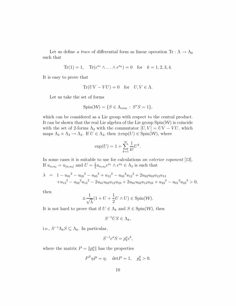
Let us define a trace of differential form as linear operation Tr : Λ → Λ0
such that
Tr(1) = 1, Tr(ea1 ∧ . . . ∧ eak) = 0 for k = 1, 2, 3, 4.
It is easy to prove that
Tr(UV − V U) = 0 for U, V ∈ Λ.
Let us take the set of forms
Spin(W) = S ∈ Λeven : S∗S = 1,
which can be considered as a Lie group with respect to the central product.It can be shown that the real Lie algebra of the Lie group Spin(W) is coincidewith the set of 2-forms Λ2 with the commutator [U, V ] = UV − V U , whichmaps Λ2 × Λ2 → Λ2. If U ∈ Λ2, then ±exp(U) ∈ Spin(W), where
exp(U) = 1 +∞∑
k=1
1
k!Uk.
In some cases it is suitable to use for calculations an exterior exponent [13].If ua1a2 = u[a1a2] and U = 1
2ua1a2e
a1 ∧ ea2 ∈ Λ2 is such that
λ = 1 − u012 − u02
2 − u032 + u12
2 − u032u12
2 + 2u02u03u12u13
+u132 − u02
2u132 − 2u01u03u12u23 + 2u01u02u13u23 + u23
2 − u012u23
2 > 0,
then
± 1√λ
(1 + U +1
2U ∧ U) ∈ Spin(W).
It is not hard to prove that if U ∈ Λk and S ∈ Spin(W), then
S−1US ∈ Λk,
i.e., S−1ΛkS ⊆ Λk. In particular,
S−1eaS = pabe
b,
where the matrix P = ‖pab‖ has the properties
PTηP = η, detP = 1, p00 > 0.
10
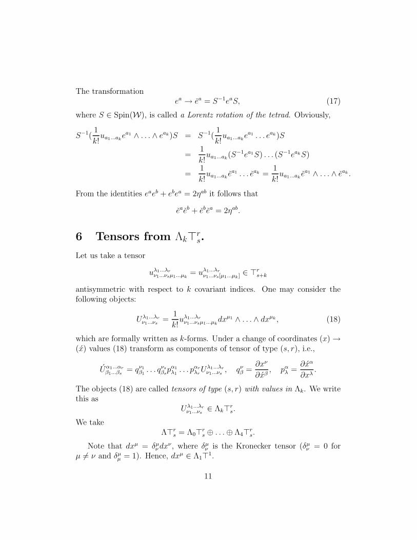
The transformationea → ea = S−1eaS, (17)
where S ∈ Spin(W), is called a Lorentz rotation of the tetrad. Obviously,
S−1(1
k!ua1...ak
ea1 ∧ . . . ∧ eak)S = S−1(1
k!ua1...ak
ea1 . . . eak)S
=1
k!ua1...ak
(S−1ea1S) . . . (S−1eakS)
=1
k!ua1...ak
ea1 . . . eak =1
k!ua1...ak
ea1 ∧ . . . ∧ eak .
From the identities eaeb + ebea = 2ηab it follows that
eaeb + ebea = 2ηab.
6 Tensors from Λk⊤rs.
Let us take a tensor
uλ1...λr
ν1...νsµ1...µk= uλ1...λr
ν1...νs[µ1...µk ] ∈ ⊤rs+k
antisymmetric with respect to k covariant indices. One may consider thefollowing objects:
Uλ1...λr
ν1...νs=
1
k!uλ1...λr
ν1...νsµ1...µkdxµ1 ∧ . . . ∧ dxµk , (18)
which are formally written as k-forms. Under a change of coordinates (x) →(x) values (18) transform as components of tensor of type (s, r), i.e.,
Uα1...αr
β1...βs= qν1
β1. . . qνs
βspα1
λ1. . . pαr
λrUλ1...λr
ν1...νs, qν
β =∂xν
∂xβ, pα
λ =∂xα
∂xλ.
The objects (18) are called tensors of type (s, r) with values in Λk. We writethis as
Uλ1...λr
ν1...νs∈ Λk⊤r
s.
We takeΛ⊤r
s = Λ0⊤rs ⊕ . . .⊕ Λ4⊤r
s.
Note that dxµ = δµν dx
ν , where δµν is the Kronecker tensor (δµ
ν = 0 forµ 6= ν and δµ
µ = 1). Hence, dxµ ∈ Λ1⊤1.
11

Elements of Λ0⊤rs are identified with tensors from ⊤r
s. For the sequel itis suitable to write tensors (18) as
Uλ1...λr
ν1...νs=
1
k!uλ1...λr
ν1...νsa1...akea1 ∧ . . . ∧ eak ∈ Λk⊤r
s.
Let us define a central product of elements Uµ1...µrν1...νs
∈ Λ⊤rs and V
α1...αp
β1...βq∈ Λ⊤p
q
as a tensor from Λ⊤r+ps+q of the form
Wµ1...µrα1...αp
ν1...νsβ1...βq= Uµ1...µr
ν1...νsV
α1...αp
β1...βq,
where on the right-hand side there is the central product of differential forms(the indices µ1, . . . , µr, α1, . . . , αp, ν1, . . . , νs, β1, . . . , βq are fixed).
If Uµ1...µrν1...νs
∈ Λ0⊤rs and V
α1...αp
β1...βq∈ Λ0⊤p
q , then the central product of theseelements is identified with the tensor product.
Let us define operators (Upsilon) Υµ, which act on tensors from Λ⊤rs by
the following rules:
a) If u = (uǫ1...ǫrν1...νs
) ∈ Λ0⊤rs, then
Υµu = ∂µu.
b) Υµdxν = −Γν
µλdxλ.
c) If U ∈ Λ⊤rs, V ∈ Λ⊤p
q, then
Υλ(UV ) = (ΥλU)V + UΥλV.
d) If U, V ∈ Λ⊤rs, then
Υλ(U + V ) = ΥλU + ΥλV.
With the aid of these rules it is easy to calculate how operators Υµ acton arbitrary tensor from Λ⊤r
s.
Theorem 1. If U ∈ Λk has the form (13), then
ΥνU =1
k!uµ1...µk;νdx
µ1 ∧ . . . ∧ dxµk ∈ Λk⊤1.
The proof in straightforward.
12
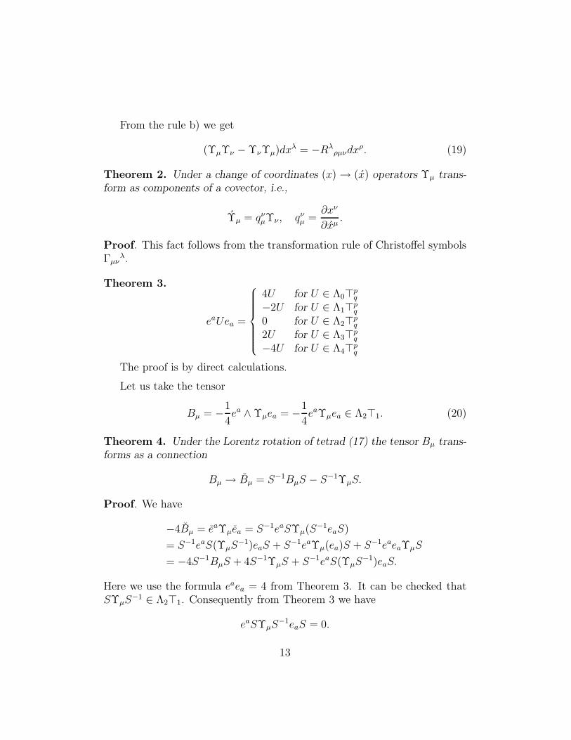
From the rule b) we get
(ΥµΥν − ΥνΥµ)dxλ = −Rλρµνdx
ρ. (19)
Theorem 2. Under a change of coordinates (x) → (x) operators Υµ trans-form as components of a covector, i.e.,
Υµ = qνµΥν , qν
µ =∂xν
∂xµ.
Proof. This fact follows from the transformation rule of Christoffel symbolsΓµν
λ.
Theorem 3.
eaUea =
4U for U ∈ Λ0⊤pq
−2U for U ∈ Λ1⊤pq
0 for U ∈ Λ2⊤pq
2U for U ∈ Λ3⊤pq
−4U for U ∈ Λ4⊤pq
The proof is by direct calculations.
Let us take the tensor
Bµ = −1
4ea ∧ Υµea = −1
4eaΥµea ∈ Λ2⊤1. (20)
Theorem 4. Under the Lorentz rotation of tetrad (17) the tensor Bµ trans-forms as a connection
Bµ → Bµ = S−1BµS − S−1ΥµS.
Proof. We have
−4Bµ = eaΥµea = S−1eaSΥµ(S−1eaS)
= S−1eaS(ΥµS−1)eaS + S−1eaΥµ(ea)S + S−1eaeaΥµS
= −4S−1BµS + 4S−1ΥµS + S−1eaS(ΥµS−1)eaS.
Here we use the formula eaea = 4 from Theorem 3. It can be checked thatSΥµS
−1 ∈ Λ2⊤1. Consequently from Theorem 3 we have
eaSΥµS−1eaS = 0.
13
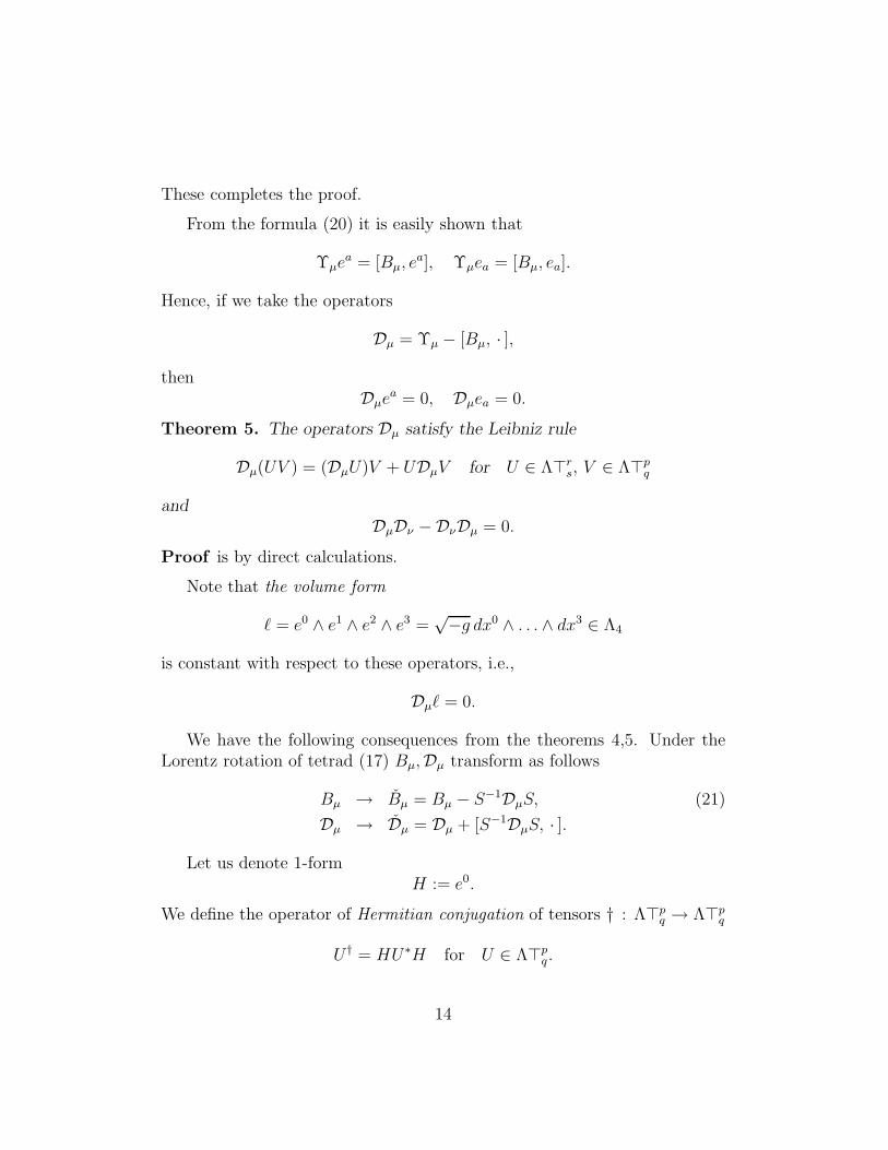
These completes the proof.
From the formula (20) it is easily shown that
Υµea = [Bµ, e
a], Υµea = [Bµ, ea].
Hence, if we take the operators
Dµ = Υµ − [Bµ, · ],
thenDµe
a = 0, Dµea = 0.
Theorem 5. The operators Dµ satisfy the Leibniz rule
Dµ(UV ) = (DµU)V + UDµV for U ∈ Λ⊤rs, V ∈ Λ⊤p
q
andDµDν −DνDµ = 0.
Proof is by direct calculations.
Note that the volume form
ℓ = e0 ∧ e1 ∧ e2 ∧ e3 =√−g dx0 ∧ . . . ∧ dx3 ∈ Λ4
is constant with respect to these operators, i.e.,
Dµℓ = 0.
We have the following consequences from the theorems 4,5. Under theLorentz rotation of tetrad (17) Bµ,Dµ transform as follows
Bµ → Bµ = Bµ − S−1DµS, (21)
Dµ → Dµ = Dµ + [S−1DµS, · ].
Let us denote 1-formH := e0.
We define the operator of Hermitian conjugation of tensors † : Λ⊤pq → Λ⊤p
q
U † = HU∗H for U ∈ Λ⊤pq .
14
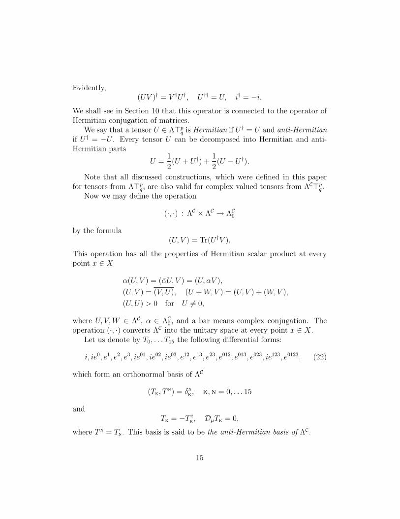
Evidently,(UV )† = V †U †, U †† = U, i† = −i.
We shall see in Section 10 that this operator is connected to the operator ofHermitian conjugation of matrices.
We say that a tensor U ∈ Λ⊤pq is Hermitian if U † = U and anti-Hermitian
if U † = −U . Every tensor U can be decomposed into Hermitian and anti-Hermitian parts
U =1
2(U + U †) +
1
2(U − U †).
Note that all discussed constructions, which were defined in this paperfor tensors from Λ⊤p
q , are also valid for complex valued tensors from ΛC⊤pq .
Now we may define the operation
(·, ·) : ΛC × ΛC → ΛC0
by the formula(U, V ) = Tr(U †V ).
This operation has all the properties of Hermitian scalar product at everypoint x ∈ X
α(U, V ) = (αU, V ) = (U, αV ),
(U, V ) = (V, U), (U +W,V ) = (U, V ) + (W,V ),
(U,U) > 0 for U 6= 0,
where U, V,W ∈ ΛC, α ∈ ΛC0 , and a bar means complex conjugation. The
operation (·, ·) converts ΛC into the unitary space at every point x ∈ X.Let us denote by T0, . . . T15 the following differential forms:
i, ie0, e1, e2, e3, ie01, ie02, ie03, e12, e13, e23, e012, e013, e023, ie123, e0123. (22)
which form an orthonormal basis of ΛC
(Tk, Tn) = δnk, k,n = 0, . . . 15
andTk = −T †
k, DµTk = 0,
where T n = Tn. This basis is said to be the anti-Hermitian basis of ΛC.
15

A differential form t ∈ ΛC such that
t2 = t, Dµt = 0, t† = t (23)
is called an idempotent. We suppose that under a Lorentz rotation of tetradea → ea = S−1eaS, S ∈ Spin(W) an idempotent t transforms as
t→ t = S−1tS.
In this case
t2 = t,
t† = Ht∗H = t,
Dµt = 0.
We may consider the left ideal generated by the idempotent t
I(t) = Ut : U ∈ ΛC ⊆ ΛC. (24)
Let us define the set of differential forms
L(t) = U ∈ I(t) : U † = −U, [U, t] = 0.
This set is closed with respect to the commutator (if U, V ∈ L(t), then[U, V ] ∈ L(t)) and can be considered as a real Lie algebra. With the aid ofthe real Lie algebra L(t) we define the corresponding Lie group
G(t) = exp(U) : U ∈ L(t).
In Section 10 we consider t, I(t), L(t), G(t) in details.Finally let us summarize properties of the operators Dµ
Dµ(UV ) = (DµU)V + UDµV,
DµDν −DνDµ = 0,
Dµ(U + V ) = DµU + DµV,
Dµea = 0, Dµea = 0,
Dµℓ = 0,
Dµ(U∗) = (DµU)∗,
Dµ(U †) = (DµU)†,
Dµ(Tr(U)) = ∂µ(Tr(U)) = Tr(DµU),
Dµ(U, V ) = ∂µ(U, V ) = (DµU, V ) + (U,DµV ).
16
Under a change of coordinates (x) → (x) operators Dµ transform as compo-nents of a covector, i.e.,
Dµ → Dµ =∂xν
∂xµDν .
Under a Lorentz rotation of tetrad ea → ea = S−1eaS (S ∈ Spin(W)) opera-tors Dµ transform as Dµ → Dµ = Dµ + [S−1DµS, · ].
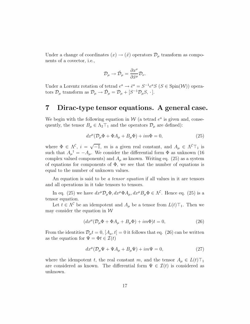
7 Dirac-type tensor equations. A general case.
We begin with the following equation in W (a tetrad ea is given and, conse-quently, the tensor Bµ ∈ Λ2⊤1 and the operators Dµ are defined):
dxµ(DµΦ + ΦAµ +BµΦ) + imΦ = 0, (25)
where Φ ∈ ΛC, i =√−1, m is a given real constant, and Aµ ∈ ΛC⊤1 is
such that Aµ† = −Aµ. We consider the differential form Φ as unknown (16
complex valued components) and Aµ as known. Writing eq. (25) as a systemof equations for components of Φ, we see that the number of equations isequal to the number of unknown values.
An equation is said to be a tensor equation if all values in it are tensorsand all operations in it take tensors to tensors.
In eq. (25) we have dxµDµΦ, dxµΦAµ, dxµBµΦ ∈ ΛC. Hence eq. (25) is a
tensor equation.Let t ∈ ΛC be an idempotent and Aµ be a tensor from L(t)⊤1. Then we
may consider the equation in W
(dxµ(DµΦ + ΦAµ +BµΦ) + imΦ)t = 0, (26)
From the identities Dµt = 0, [Aµ, t] = 0 it follows that eq. (26) can be writtenas the equation for Ψ = Φt ∈ I(t)
dxµ(DµΨ + ΨAµ +BµΨ) + imΨ = 0, (27)
where the idempotent t, the real constant m, and the tensor Aµ ∈ L(t)⊤1
are considered as known. The differential form Ψ ∈ I(t) is considered asunknown.
17

In Section 10 we shall see that there are four types of idempotents t.Consequently, there are four types of equations (27). These equations arecalled Dirac-type tensor equations. A connection of eqs. (27) with the Diracequation will be discussed in Section 9.
Denoting αµ = Hdxµ ∈ (Λ0 ⊕ Λ2)⊤1, we see that (αµ)† = αµ.
Theorem 6. If Ψ ∈ I(t) satisfies eq. (27), then the tensor
Jµ = iΨ†αµΨ
satisfies the equality
1√−gDµ(√−g Jµ) − [Aµ, J
µ] = 0, (28)
which is called a (non-Abelian) charge conservation law.
Note that Ψ = Ψt and Jµ = tJµt. Therefore,
[Jµ, t] = [tJµt, t] = 0,
i.e., Jµ ∈ L(t)⊤1.
Proof of Theorem 6. Let us multiply eq. (26) from the left by H and denotethe left-hand side of resulting equation by
Q = αµ(DµΨ + ΨAµ +BµΨ) + imHΨ. (29)
ThenQ† = (DµΨ† − AµΨ† + Ψ†B†
µ)αµ − imΨ†H.
Consider the expression
i(Ψ†Q+Q†Ψ) = i(Ψ†αµDµΨ + DµΨ†αµΨ + Ψ†(Dµαµ)Ψ) − [Aµ, iΨ
†αµΨ]
+iΨ†(−Dµαµ + αµBµ +B†
µαµ)Ψ (30)
=1√−gDµ(
√−g Jµ) − [Aµ, Jµ].
Here we use the formulae
Dµαµ = −Γµν
µαν + αµBµ +B†µα
µ,
DµJµ + Γµν
µJν =1√−gDµ(
√−g Jµ).
18

which can be easily checked. In (30) equality Q = 0 leads to the equality(28). These completes the proof.
Now we may write eq. (27) together with Yang-Mills equations (32,33)
dxµ(DµΨ + ΨAµ +BµΨ) + imΨ = 0, (31)
DµAν −DνAµ − [Aµ, Aν ] = Fµν , (32)
1√−gDµ(√−g F µν) − [Aµ, F
µν ] = Jν , (33)
Jν = iΨ†ανΨ, (34)
where Ψ ∈ I(t), Aµ ∈ L(t)⊤1, Fµν ∈ L(t)⊤2, Jν ∈ L(t)⊤1. In this system ofequations we consider Ψ, Aµ, Fµν , J
ν as unknown values and m, t as knownvalues.
Theorem 7. Let us denote the left-hand side of eq. (33) by Rν
Rν :=1√−gDµ(
√−g F µν) − [Aµ, Fµν ],
where Fµν satisfy (32). Then
1√−gDµ(√−g Rµ) − [Aµ, R
µ] = 0.
The proof is by direct calculations.
This theorem means that eq. (33) is consistent with the charge conser-vation law (28).
8 Unitary and Spin gauge symmetries.
Theorem 8. Let Ψ, Aµ, Fµν , Jν satisfy eqs. (31-34) with a given idempotent
t and constant m. And let U ∈ G(t), where the Lie group G(t) is defined inSection 6. Then the following values with tilde:
Ψ = ΨU, Aµ = U−1AµU − U−1DµU, Fµν = U−1FµνU,
Jν = U−1JνU, t, Bµ, Dµ = t, Bµ,Dµsatisfy the same equations (31-34).
The proof is straightforward.
This theorem means that eqs. (31-34) are invariant under gauge trans-formations with the symmetry Lie group G(t).
19

Theorem 9. Let Ψ, Aµ, Fµν , Jν satisfy eqs. (31-34) with a given idempotent
t and constant m. And let S ∈ Spin(W). Then the following values withcheck:
Ψ = ΨS, Aµ = S−1AµS, Fµν = S−1FµνS, Jν = S−1JνS, (35)
t = S−1tS, Bµ = Bµ − S−1DµS, Dµ = Dµ + [S−1Dµ, · ]satisfy the same equations (31-34).
The proof is by direct calculations.
Note that for values with check the operation of Hermitian conjugationis defined by U † = HU∗H , where H = S−1HS.
This theorem means that eqs. (31-34) are invariant under gauge trans-formations with the symmetry Lie group Spin(W).
Eqs. (31-34) can be derived from the following Lagrangian:
L =1
4i√−gTr(Ψ†HQ−Q†HΨ) + C
1
4
√−g Tr(1
8FµνF
µν), (36)
where Q is from (29), Fµν = DµAν −DνAµ − [Aµ, Aν ] ∈ L(t)⊤2, and C is areal constant. If we have a basis t1, . . . , tD of I(t) and a basis τ1, . . . , τdof L(t) that satisfy (37),(42), then we may substitute Ψ = ψktk, Aµ = an
µτninto the Lagrangian L. Variating L with respect to ψk and an
µ, we arrive ateqs. (31-34). We discuss bases of I(t) and L(t) in Section 10.
In [4] we discuss a gravitational term for the Lagrangian L.
9 A connection between the Dirac-type ten-
sor equation and the Dirac equation.
Let t ∈ ΛC be an idempotent with the properties (23) and I(t) be the leftideal (24) of complex dimension D. In the next section we shall see that Dmay take one of four possible values D = 4, 8, 12, 16. We use an orthonormalbasis tk = tk, k = 1, . . . , D of I(t) such that
Dµtk = 0, (tn, tk) = δkn . (37)
Small Caps font indices run from 1 to D. Consider a linear operator |〉that maps I(t) to CD. If
Ω = ωktk ∈ I(t),
20
then|Ω〉 = (ω1 . . . ωD)T.
In particular,|tk〉 = (0 . . . 1 . . . 0)T
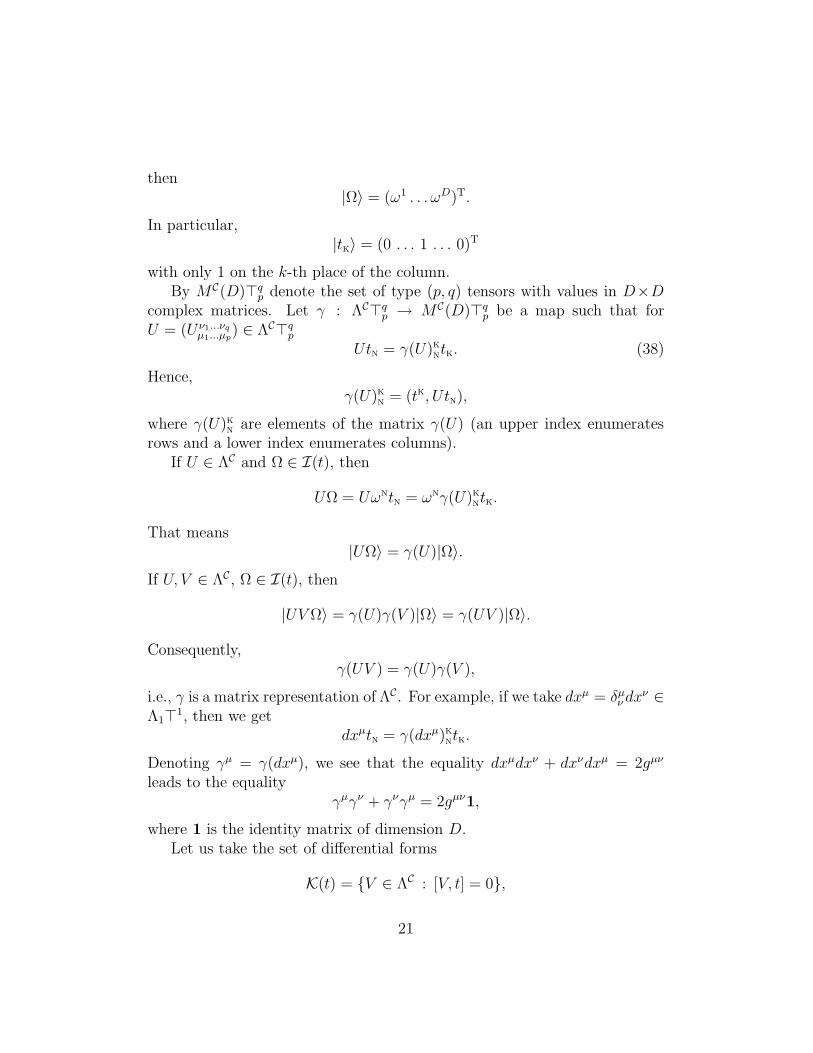
with only 1 on the k-th place of the column.By MC(D)⊤q
p denote the set of type (p, q) tensors with values in D×Dcomplex matrices. Let γ : ΛC⊤q
p → MC(D)⊤qp be a map such that for
U = (Uν1...νqµ1...µp
) ∈ ΛC⊤qp
Utn = γ(U)kntk. (38)
Hence,γ(U)kn = (tk, Utn),
where γ(U)kn
are elements of the matrix γ(U) (an upper index enumeratesrows and a lower index enumerates columns).
If U ∈ ΛC and Ω ∈ I(t), then
UΩ = Uωntn = ωnγ(U)kntk.
That means|UΩ〉 = γ(U)|Ω〉.
If U, V ∈ ΛC, Ω ∈ I(t), then
|UV Ω〉 = γ(U)γ(V )|Ω〉 = γ(UV )|Ω〉.
Consequently,γ(UV ) = γ(U)γ(V ),
i.e., γ is a matrix representation of ΛC. For example, if we take dxµ = δµν dx
ν ∈Λ1⊤1, then we get
dxµtn = γ(dxµ)kntk.
Denoting γµ = γ(dxµ), we see that the equality dxµdxν + dxνdxµ = 2gµν
leads to the equalityγµγν + γνγµ = 2gµν1,
where 1 is the identity matrix of dimension D.Let us take the set of differential forms
K(t) = V ∈ ΛC : [V, t] = 0,
21

which can be considered as an algebra (at any point x ∈ X). Now we definea map
θ : K(t)⊤qp → MC(D)⊤q
p
such that for V = (V ν1...νqµ1...µp
) ∈ K(t)⊤qp
tnV = θ(V )kntk.
Therefore,θ(V )k
n= (tk, tnV ).
If V ∈ K(t) and Ω ∈ I(t), then
ΩV = ωntnV = ωnθk
ntk.
Than means|ΩV 〉 = θ(V )|Ω〉.
If U, V ∈ K(t), Ω ∈ I(t), then
|ΩUV 〉 = θ(V )θ(U)|Ω〉 = θ(UV )|Ω〉.
Consequently,θ(UV ) = θ(V )θ(U).
If U ∈ ΛC, V ∈ K(t), Ω ∈ I(t), then UΩ ∈ I(t), ΩV ∈ I(t) and
|UΩV 〉 = γ(U)|ΩV 〉 = γ(U)θ(V )|Ω〉,|UΩV 〉 = θ(V )|UΩ〉 = θ(V )γ(U)|Ω〉.
Consequently,[γ(U), θ(V )] = 0.
Denoting the left-hand side of eq. (27) by
Ω = dxµ(DµΨ + ΨAµ +BµΨ) + imΨ (39)
and using formulas
ψ := |Ψ〉,|DµΨ〉 = |Dµ(tkψ
k)〉 = |tk∂µψk〉 = ∂µψ,
|dxµΨAµ〉 = γµ|ΨAµ〉 = γµθ(Aµ)ψ,
|dxµBµΨ〉 = γµ|BµΨ〉 = γµγ(Bµ)ψ,
22

we see that|Ω〉 = γµ(∂µ + θ(Aµ) + γ(Bµ))ψ + imψ. (40)
Note that
Bµ =1
2bµabe
a ∧ eb =1
4bµab(e
aeb − ebea).
Therefore,
γ(Bµ) =1
4bµab[γ
a, γb],
where γa = γ(ea) and the equalities eaeb + ebea = 2ηab leads to the equalities
γaγb + γbγa = 2ηab1.
If we take V ∈ G(t), then
ΩV = (dxµ(DµΨ + ΨAµ +BµΨ) + imΨ)V
= dxµ(Dµ(ΨV ) + ΨV (V −1AµV − V −1DµV ) +Bµ(ΨV )) + im(ΨV )
and
|ΩV 〉 = θ(V )|Ω〉 = P (γµ(∂µ + θ(Aµ) + γ(Bµ))ψ + imψ)
= γµ(∂µ + (Pθ(Aµ)P−1 − (∂µP )P−1) + γ(Bµ))(Pψ) + imPψ,
where P = θ(V ) and we use formulae [P, γµ] = 0, [P, γ(Bµ)] = 0. Thus theinvariance of eq. (27) under the gauge transformation (V ∈ G(t))
Ψ → ΨV, Aµ → V −1AµV − V −1DµV
leads to the invariance of the equation
γµ(∂µ + θ(Aµ) + γ(Bµ))ψ + imψ = 0 (41)
under the gauge transformation (P = θ(V ))
ψ → Pψ, θ(Aµ) → Pθ(Aµ)P−1 − (∂µP )P−1.
Let S ∈ Spin(W). Consider the Lorentz rotation of the tetrad ea → ea =S−1eaS, which leads to the transformation
t→ t = S−1tS, I(t) → I(t), tn → tn = S−1tnS.
23

Let us define a map |〉 : I(t) → CD. If Φ = φktk ∈ I(t), then
|Φ〉 = (φ1 . . . φD)T.
Evidently for Ω ∈ I(t)|S−1ΩS 〉 = |Ω〉.
Also we may define a map γ : ΛC⊤qp →MC(D)⊤q
p such that
Utn = γ(U)kn tk
andγ(UV ) = γ(U)γ(V ).
It is easily seen thatγ(U) = γ(S)γ(U)γ(S−1).
In particular,γ(S) = γ(S).
For Ω ∈ I(t) we have
|ΩS 〉 = |S(S−1ΩS)〉 = γ(S)|S−1ΩS 〉 = γ(S)|Ω〉.
If we apply these identities to
ΩS = (dxµ(DµΨ + ΨAµ +BµΨ) + imΨ)S
= dxµ(DµΨ + ΨAµ + BµΨ) + imΨ,
then we get
|ΩS 〉 = γ(S)|Ω〉 = R(γµ(∂µψ + θ(Aµ)ψ + γ(Bµ)ψ) + imψ)
= RγµR−1(∂µ(Rψ) + θ(Aµ)Rψ + (Rγ(Bµ)R−1 − (∂µR)R−1)Rψ) + imRψ,
where R = γ(S). Note that [R, θ(Aµ)] = 0.This implies that the invariance of eq. (27) under the gauge transforma-
tion (35) leads to the invariance of eq. (41) under the gauge transformation(R = γ(S))
ψ → Rψ, θ(Aµ) → θ(Aµ) γµ → RγµR−1,
γ(Bµ) → Rγ(Bµ)R−1 − (∂µR)R−1.
24

Now consider a transformation of eqs. (27),(41) under a change of coor-dinates (x) → (x). Coordinates (x) we denote with the aid of primed indicesxµ′
. In coordinates (x) eq. (27) has the form
Ω ≡ dxµ′
(Dµ′Ψ + ΨAµ′ +Bµ′Ψ) + imΨ = 0,
where
Dµ′ =∂xν
∂xµ′Dν , dxµ′
=∂xµ′
∂xνdxν , Aµ′ =
∂xν
∂xµ′Aν , Bµ′ =
∂xν
∂xµ′Bν ,
and eq. (41) has the form
|Ω〉 = γµ′
(∂µ′ + θ(Aµ′) + γ(Bµ′))ψ + imψ = 0,
where
∂µ′ =∂
∂xµ′, γµ′
=∂xµ′
∂xνγν .
Note thatγµ = γ(dxµ) = γaeµ
a, γa = γ(ea)
and
γµ′
= γaeµ′
a = γa∂xµ′
∂xνeν
a.
Finally, let us note that in the Lagrangian (36)
1
4
√−g Tr(i(Ψ†HΩ − Ω†HΨ)) =
1
4
√−g i(〈Ψ|γ0|Ω〉 − 〈Ω|γ0|Ψ〉),
where 〈Ψ| = |Ψ〉†.
10 Idempotents and bases of left ideals.
Let us take the idempotent
t(1) =1
4(1 + e0)(1 + ie12) =
1
4(1 + e0 + ie12 + ie012),
which satisfies conditions (23), and consider the left ideal I(t(1)). It can beshown that the complex dimension of I(t(1)) is equal to four (this I(t(1)) is a
25

minimal left ideal of ΛC and t(1) is a primitive idempotent) and the followingdifferential forms
t1 = 2t(1) =1
2(1 + e0 + ie12 + ie012),
t2 = −2e13t(1) =1
2(−e13 + ie23 − e013 + ie023),
t3 = 2e03t(1) =1
2(−e3 + e03 − ie123 + ie0123),
t4 = 2e01t(1) =1
2(−e1 + ie2 + e01 − ie02)
can be taken as basis forms of I(t(1)), which satisfy (37). This basis, accordingto the formula (38), defines the matrix representation of ΛC (γ(1) is a one-to-one map)
γ(1) : ΛC⊤qp →MC⊤q
p.
In particular we get matrices γµ(1) = γ(1)(dx
µ) identical to (2). Denote
U := γ(1)(U) for U ∈ ΛC⊤qp.
Let Y n
k∈ ΛC, (k,n = 1, 2, 3, 4) be differential forms such that Y n
kare 4×4-
matrices with only nonzero element that equal to 1 on the intersection ofn-th row and k-th column. We can calculate that
Y 11 = (1 + e0 + e012i+ e12i)/4,
Y 12 = (e013 + e13 + e023i + e23i)/4,
Y 13 = (e03 + e3 + e0123i+ e123i)/4,
Y 14 = (e01 + e1 + e02i+ e2i)/4,
Y 21 = (−e013 − e13 + e023i + e23i)/4,
Y 22 = (1 + e0 − e012i− e12i)/4,
Y 23 = (e01 + e1 − e02i− e2i)/4,
Y 24 = (−e03 − e3 + e0123i + e123i)/4,
Y 31 = (e03 − e3 + e0123i− e123i)/4,
Y 32 = (e01 − e1 + e02i− e2i)/4,
Y 33 = (1 − e0 − e012i+ e12i)/4,
Y 34 = (−e013 + e13 − e023i + e23i)/4,
Y 41 = (e01 − e1 − e02i+ e2i)/4,
26
Y 42 = (−e03 + e3 + e0123i− e123i)/4,
Y 43 = (e013 − e13 − e023i+ e23i)/4,
Y 44 = (1 − e0 + e012i− e12i)/4.
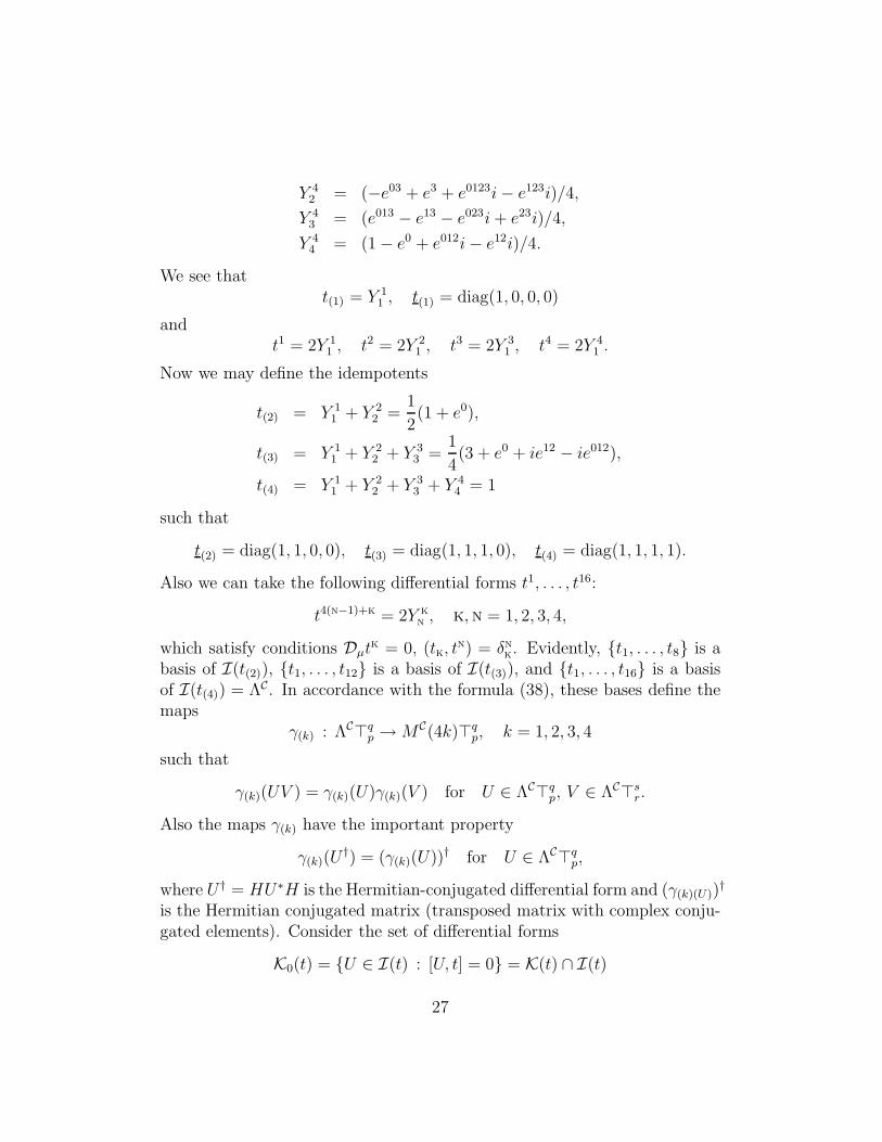
We see thatt(1) = Y 1
1 , t(1) = diag(1, 0, 0, 0)
andt1 = 2Y 1
1 , t2 = 2Y 21 , t3 = 2Y 3
1 , t4 = 2Y 41 .
Now we may define the idempotents
t(2) = Y 11 + Y 2
2 =1
2(1 + e0),
t(3) = Y 11 + Y 2
2 + Y 33 =
1
4(3 + e0 + ie12 − ie012),
t(4) = Y 11 + Y 2
2 + Y 33 + Y 4
4 = 1
such that
t(2) = diag(1, 1, 0, 0), t(3) = diag(1, 1, 1, 0), t(4) = diag(1, 1, 1, 1).
Also we can take the following differential forms t1, . . . , t16:
t4(n−1)+k = 2Y k
n , k,n = 1, 2, 3, 4,
which satisfy conditions Dµtk = 0, (tk, t
n) = δnk. Evidently, t1, . . . , t8 is a
basis of I(t(2)), t1, . . . , t12 is a basis of I(t(3)), and t1, . . . , t16 is a basisof I(t(4)) = ΛC. In accordance with the formula (38), these bases define themaps
γ(k) : ΛC⊤qp →MC(4k)⊤q
p, k = 1, 2, 3, 4
such that
γ(k)(UV ) = γ(k)(U)γ(k)(V ) for U ∈ ΛC⊤qp, V ∈ ΛC⊤s
r.
Also the maps γ(k) have the important property
γ(k)(U†) = (γ(k)(U))† for U ∈ ΛC⊤q
p,
where U † = HU∗H is the Hermitian-conjugated differential form and (γ(k)(U))†
is the Hermitian conjugated matrix (transposed matrix with complex conju-gated elements). Consider the set of differential forms
K0(t) = U ∈ I(t) : [U, t] = 0 = K(t) ∩ I(t)
27
and the corresponding set of 4×4-matrices
K0(t) = U : U ∈ K0(t).
Evidently K0(t(k)), (k = 1, 2, 3, 4) are sets of matrices with all zero elementsexcept elements in the left upper k×k-block.
Considering the sets of differential forms
L(t(k)) = U ∈ K0(t(k)) : U † = −U
and the corresponding sets of matrices L(t(k)) as real Lie algebrae, we seethat
L(t(k)) ≃ L(t(k)) ≃ u(k) ≃ u(1) ⊕ su(k),
where u(k), (k = 1, 2, 3, 4) are Lie algebrae of anti-Hermitian k×k-matrices,su(k) are the Lie algebrae of traceless anti-Hermitian matrices, and the sign≃ denote isomorphism. We have the Lie groups
G(t(k)) ≃ G(t(k)) ≃ U(1) ⊕ SU(k),
where SU(k) are the Lie groups of unitary k×k-matrices with determinantsequal to 1.
For elements of L(t(k)) we define the normalized scalar product
(u, v)(k) :=4
k(u, v)
such that(it(k), it(k))(k) = 1, k = 1, 2, 3, 4.
Now we show that for every k = 1, 2, 3, 4 we may take generators τ of L(t(k))such that
Dµτn = 0, (τn, τm)(k) = δm
n , τ †n = −τn, [τn, τl] = cmnlτm, (42)
where τn = τn and cmnl are real structure constants of the Lie algebra L(t(k)).We use differential forms
λ1 = Y 12 + Y 2
1
λ2 = −iY 12 + iY 2
1
λ3 = Y 11 − Y 2
2
28
λ4 = Y 13 + Y 3
1
λ5 = −iY 13 + iY 3
1
λ6 = Y 23 + Y 3
2
λ7 = −iY 23 + iY 3
2
λ8 =1√3
(Y 11 + Y 2
2 − 2Y 33 )
such that λ1, . . . , λ8 is equivalent to the Gell-Mann basis of the real Liealgebra su(3). We take the following generators of L(t(k)):
1. For L(t(1)) ≃ u(1)τ0 = it(1).
2. For L(t(2)) ≃ u(1) ⊕ su(2)
τ0 = it(2), τn = iλn, n = 1, 2, 3.
3. For L(t(3)) ≃ u(1) ⊕ su(3)
τ0 = it(3), τn = i
√
3
2λn, n = 1, . . . , 8.
4. For L(t(4)) ≃ u(1)⊕ su(4) we take as a basis τ0, . . . , τ15 the anti-Hermitianbasis (22)
Therefore,L(t(k)) = fnτ
n,where fn = fn(x) are real valued scalar functions.
Let us define the set of differential forms
L(t)︸ ︷︷ ︸
= U ∈ L(t) : TrU = 0.
We see thatL(t(k))︸ ︷︷ ︸
≃ su(k), k = 2, 3, 4.
If we replace L(t) by L(t)︸ ︷︷ ︸
in above considerations, then we get that all results
are valid (we must take Jµ = iΨ†αµΨ−Tr(iΨ†αµΨ) in Theorem 6 and in eq.(34)).
29
11 Special cases
Let us denoteI = −ie12.
Then
t(1) =1
4(1 +H)(1 − iI)
andit(1) = It(1).
Theorem 10. For a given Φ ∈ I(t(1)) the equation
Ψt(1) = Φ, (43)
has a unique solution Ψ ∈ Λeven.
Proof. We have the orthonormal basis of I(t(1))
tk = Fkt(1), k = 1, 2, 3, 4,
where Fk ∈ Λeven. Decomposing Φ ∈ I(t(1)) with respect to the basis tk
Φ = (αk + iβk)tk, αk, βk ∈ Λ0, (44)
and using the relation it(1) = It(1), we see that the differential form
Ψ = Fk(αk + Iβk) ∈ Λeven
is a solution of eq. (43).We claim that if
U = u+u01e01 +u02e
02 +u03e03 +u12e
12 +u13e13 +u23e
23 +u0123e0123 ∈ Λeven
is a solution of the homogeneous equation
Ut(1) = 0,
then U = 0. Indeed, the differential form Ut(1) ∈ I(t(1)) can be decomposedinto the basis tk
Ut(1) =1
2(u− iu12)t1 +
1
2(−u13 − iu23)t2 +
1
2(u03 − iu0123)t3 +
1
2(u01 + iu02)t4.
Thus the identity Ut(1) = 0 implies U = 0. So the solution (44) of eq. (43)is unique. These completes the proof.
30
Theorem 11. For a given Φ ∈ I(t(2)) the equation
Ψt(2) = Φ, (45)
has a unique solution Ψ ∈ ΛCeven.
Proof. We have the orthonormal basis of I(t(2))
tk = Fkt(2), k = 1, . . . , 8,
where Fk ∈ ΛCeven. Decomposing Φ ∈ I(t(2)) with respect to the basis tk
Ψ = (αk + iβk)tk, αk, βk ∈ Λ0, (46)
we see that the differential form
Ψ = Fk(αk + iβk) ∈ ΛCeven
is a solution of eq. (45).We claim that if
U = (v + iw) +∑
0≤a<b≤3
(vab + iwab)eab + (v0123 + iw0123)e0123
is a solution of the homogeneous equation
Ut(2) = 0,
then U = 0. Indeed, the differential form Ut(2) ∈ I(t(2)) can be decomposedinto the basis tk
Ut(2) = φktk, φk = (tk, Ut(2)).
We get
φ1 = (v − iv12 + iw + w12)/2
φ2 = (−v13 − iv23 − iw13 + w23)/2
φ3 = (v03 − iv0123 + iw03 + w0123)/2
φ4 = (v01 + iv02 + iw01 − w02)/2
φ5 = (v13 − iv23 + iw13 + w23)/2
φ6 = (v + iv12 + iw − w12)/2
φ7 = (v01 − iv02 + iw01 + w02)/2
φ8 = (−v03 − iv0123 − iw03 + w0123)/2.
31

Evidently the identity Ut(2) = 0 implies U = 0. So the solution (46) of eq.(45) is unique. These completes the proof.
Denote1
L (t) = U ∈ Λeven : U † = −U, [U, t(1)] = 0.
The Lie algebra1
L (t) is isomorphic to the Lie algebra u(1) and as a generator
of1
L (t) we may take τ0 = I.
Theorem 12. Differential forms1
Ψ∈ Λeven,1
Aµ∈1
L (t)⊤1 satisfy the equation
dxµ(Dµ
1
Ψ +1
Ψ1
Aµ +Bµ
1
Ψ)H +m1
Ψ I = 0 (47)
iff differential forms Ψ =1
Ψ t(1) ∈ I(t(1)), Aµ =1
Aµ t(1) ∈ L(t)⊤1 satisfy eq.(27).
Proof. Multiplying (47) from the right by t(1) and using relations Ht(1) =
t(1), It(1) = it(1), we obtain that Ψ =1
Ψ t(1), Aµ =1
Aµ t(1) satisfy (27).Conversely, let Ψ ∈ I(t), Aµ ∈ L(t)⊤1 satisfy (27). By Theorem 10 there
exists a unique solution1
Ψ∈ Λeven,1
Aµ∈ Λeven⊤1 of the system of equations1
Ψ t(1) = Ψ,1
Aµ t(1) = Aµ. It can be shown that1
Aµ∈1
L (t)⊤1. Substituting1
Ψ t(1),1
Aµ t(1) for Ψ, Aµ in (27), we arrive at the equality
(dxµ(Dµ
1
Ψ +1
Ψ1
Aµ +Bµ
1
Ψ)H +m1
Ψ I)t(1) = 0,
which we rewrite as1
Ω t(1) = 0.
We see that1
Ω∈ Λeven and, according to Theorem 10, we get
1
Ω= 0.
These completes the proof.
Denote2
L (t) = U ∈ ΛCeven : U † = −U, [U, t(2)] = 0.
32

The Lie algebra2
L (t) is isomorphic to the Lie algebra u(1) ⊕ su(2) and we
may take the following generators of2
L (t):
τ0 = i, τ1 = e23, τ2 = −e13, τ3 = e12.
Theorem 13. Differential forms2
Ψ∈ ΛCeven,
2
Aµ∈2
L (t)⊤1 satisfy the equation
dxµ(Dµ
2
Ψ +2
Ψ2
Aµ +Bµ
2
Ψ)H + im2
Ψ= 0 (48)
iff differential forms Ψ =2
Ψ t(2) ∈ I(t(2)), Aµ =2
Aµ t(2) ∈ L(t)⊤1 satisfy eq.(27).
Proof is word for word identical to the proof of the preceding theorem.
Equations (47),(48) together with correspondent Yang-Mills equationswere considered in [2]-[4].
References
[1] Dirac P.A.M., Proc. Roy. Soc. Lond. A117 (1928) 610.
[2] Marchuk N.G., Nuovo Cimento, 117B, 01, (2002) 95.
[3] Marchuk N.G., Nuovo Cimento, 117B, 05, (2002) 613.
[4] Marchuk N.G., Dirac-type tensor equations on a parallelisable manifold,to appear in Nuovo Cimento B.
[5] Marchuk N.G., Nuovo Cimento, 115B, N.11, (2000) 1267.
[6] Ivanenko D., Landau L., Z. Phys., 48 (1928)340.
[7] Kahler E., Randiconti di Mat. (Roma) ser. 5, 21, (1962) 425.
[8] Riesz M., pp.123-148 in C.R. 10 Congres Math. Scandinaves, Copen-hagen, 1946. Jul. Gjellerups Forlag, Copenhagen, 1947. Reprintedin L.Garding, L.Hermander (eds.): Marcel Reisz, Collected Papers,Springer, Berlin, 1988, pp.814-832.
[9] Gursey F., Nuovo Cimento, 3, (1956) 988.
33
[10] Hestenes D., Space-Time Algebra, Gordon and Breach, New York, 1966.
[11] Hestenes D., J. Math. Phys., 8, (1967) 798-808.
[12] Benn I.M., Tucker R.W., An introduction to spinors and geometry withapplications to physics, Bristol, 1987.
[13] Lounesto P., Clifford Algebras and Spinors, Cambridge Univ. Press(1997, 2001)
[14] Grassmann H., Math. Commun. 12, 375 (1877).
[15] Doran C., Hestenes D., Sommen F., Van Acker N., J.Math.Phys. 34(8),(1993) 3642.
34