EC

B

EZ

B

EK

T

BC

E

EK

P

WO R K I N G PA P E R S E R I E S

WORKING PAPER NO. 7

A CROSS-COUNTRY COMPARISON

OF MARKET STRUCTURES

IN EUROPEAN BANKING

BY

OLIVIER DE BANDT

AND E. PHILIP DAVIS

SEPTEMBER 1999

EC

B

EZ

B

EK

T

BC

E

EK

P

WO R K I N G PA P E R S E R I E S

WORKING PAPER NO. 7

A CROSS-COUNTRY COMPARISON OF MARKET STRUCTURESIN EUROPEAN BANKING*

BYOLIVIER DE BANDT

AND E. PHILIP DAVIS

SEPTEMBER 1999

* Olivier De Bandt is a senior economist at the Banque de France. E Philip Davis is a senior economist at the Bank of England. Both were formerly on secondment to the European Central Bank(ECB), in particular when most of the paper was drafted. Davis is also a Research Associate of the LSE Financial Markets Group, Associate Fellow of the Royal Institute of International Affairs andResearch Fellow of the Pensions Institute at Birkbeck College, London. Views expressed are those of the authors and not necessarily those of the ECB, the Bank of England or the Banque de France.They thank Salvatore Marrocco for excellent research assistance. They are also grateful to Ignazio Angeloni, Ted Gardener, Phil Molyneux, Philippe Moutot and Patrick Sevestre, as well as seminarparticipants in Bangor, Rome (Tor Vergata), at the Bank of England and the ECB for helpful comments.

© European Central Bank, 1999

Address Kaiserstrasse 29

D-60311 Frankfurt am Main

GERMANY

Postal address Postfach 16 03 19

D-60066 Frankfurt am Main

Germany

Telephone +49 69 1344 0

Internet http://www.ecb.int

Fax +49 69 1344 6000

Telex 411 144 ecb d

All rights reserved.

Reproduction for educational and non-commercial purposes is permitted provided that the source is acknowledged.

The views expressed in this paper are those of the author and do not necessarily reflect those of the European Central Bank.

ISSN 1561-0810

Abstract

In order to assess the effect of EMU on market conditions for banks based in countries

which adopt the Single Currency, we use the H indicator suggested by Panzar and Rosse

(1987). Our contribution is to assess results separately for large and small banks, and for

interest income and total income as a dependent variable. From a panel of banks over the

period 1992-1996, we provide evidence that European banking markets for large banks in

the mid-1990s were still characterised by monopolistic competition, as compared to the

United States. Regarding small banks, the level of competition appears to be even lower,

especially in France and Germany. EMU would therefore imply a notable rise in

competition for small banks in France and Germany, as well as an increase in competition

for large banks, especially in Italy.

JEL Classification: G21, L12

2

Introduction

It is widely agreed that EMU will significantly affect the degree of competition in the

banking sectors of countries adopting the Single Currency, due inter alia to heightened

disintermediation and increased actual and potential cross-border competition. These

tendencies are expected to put banks’ profitability under significant downward pressure and

enhance forces leading to restructuring and consolidation. In this context, we estimate

equations which cast light on recent levels in banking market competition, so as, first, to

provide a benchmark against which the effect of EMU may be assessed. Corresponding

results for a deregulated and continental banking system – potentially akin to EMU - are

also derived for the United States. The methodology involves the estimation of revenue

functions and consideration of the so-called H statistic, which is the sum of elasticities of

revenue to the components of expenditure. One innovation of the paper is that competitive

conditions are estimated both in terms of interest income and total income. This is

considered to be highly relevant given that banks are seeking non-interest revenue as a

supplement to declining interest income as deregulation and structural change proceeds. For

example, OECD data show that non-interest income has accounted in recent years for 20-

40% of total net income in the countries studied. Moreover, we assess results separately for

large and small banks, which may face different competitive conditions.

The paper is structured as follows: in the first section we seek briefly to motivate the

analysis by consideration of how structural changes in the past and the future impact of

EMU is considered to affect banks. In the second we provide details of the methodology of

the paper. The third describes the data sources employed, and the fourth gives the main

results. The final section draws conclusions.

1 Underlying trends and the consequences of EMU

In many OECD countries, the banking industry has for some time been in a state of change,

with banks facing heightened competition both within and outside the industry. This has in

turn had an impact on banking behaviour and banking market structure. Deregulation,

advances in technology and the growth of institutional investors and securities markets are

among the most important causes of this pattern. Whereas these tendencies were observed

most acutely at an early stage in the Anglo-Saxon countries, and later in Japan and the

Nordic countries, they have increasingly made themselves felt in Continental Europe, not

least as a consequence of the Single Market programme. This section briefly recalls in

3

general terms the main developments seen in the past, before outlining how EMU may

amplify these effects in the future.

Both in Europe and elsewhere, the growth of domestic and international capital markets

(linked partly to the rise of institutional investors) encouraged highly-rated corporate

borrowers to shift much of their demand for debt finance from banks to markets, leaving the

former with higher-risk credits. Securitised assets also met with strong demand from

institutional investors. Abolition of exchange controls meant that demand for securities and

securitised assets became global and was not limited to institutional investors from the

country concerned.

In addition, the scope of public as opposed to private information and the efficiency of its

use by markets was increased by the development of information technology and the related

growth in influence of rating agencies, investment banks and credit assessors covering a

wider range of firms. The traditional comparative advantages of banks in this area resulting

from economies of scale in information gathering, screening and monitoring (Diamond,

1984) were thus eroded, even abstracting from price considerations. Meanwhile on the

liabilities side of banks’ balance sheets, wholesale depositors such as corporate treasurers

and institutional investors tended to be ready customers for repos, commercial paper and

other money market instruments rather than bank deposits - and individuals had attractive

opportunities to hold money market funds1 - in each case undermining banks' comparative

advantage in liquidity provision (Dermine, 1991). Both of these trends are leading to a

decline in banks’ traditional on-balance sheet business.

Such disintermediation was combined with financial liberalisation – and in particular for

Europe the Single Market Programme - innovations and technical developments that

enhanced competition also for traditional banking products such as mortgages, consumer

credit and deposits (Vives, 1991), between domestic and foreign banks, vis-à-vis non-bank

financial institutions (notably insurance companies) and with non financial players such as

department stores and car companies. Together with capital market disintermediation, these

impacted strongly on banks' margins and made it difficult for banks to operate with their

traditional mix of business alone. In effect, banks were left with a problem of “excess

capacity” owing to the shift towards a more competitive market (Davis and Salo, 1998).

1 The public also had the option of holding public debt which offered high yields relative to bankdeposits.

4

Banks responded partly by increasing their focus on non-interest income – including asset

management income per se, mutual funds and insurance – and reducing excess capacity by

merger or branch closure. Note in this context that EU banks are freer to engage in a broad

range of activities than has traditionally been the case in the US or Japan; and the Single

Market Directives such as the Second Bank Co-ordination Directive (2BCD) increased this

scope further. For example, since 2BCD, banks have been allowed to enter the capital

markets in a number of EU countries. Increased focus on competitive strengths and

improved services were another response; in effect, some banks sought to specialise in

activities where they have a comparative advantage, including traditional retail banking per

se. However, disintermediation historically also led at times to increased risk-taking via

aggressive balance sheet expansion (e.g. by lending to Latin America, property developers,

and more recently Asian borrowers, Russia and hedge funds) with risk premia which in

retrospect proved to be inadequate2. Ill-advised cross border ventures, which often proved

unprofitable, were often a part of this pattern.

Turning to EMU, in respect of banks, the bulk of commentaries on the financial market

consequences of EMU (see for example, Dermine (1996), IMF (1997) and McCauley and

White (1997), De Bandt (1999), ECB (1999)) are that it will have the following effects on

banks and banking competition:

From a structural point of view, disintermediation may increase after EMU via the

following channels:

• increased attractiveness of commercial paper, bond and equity finance to companies

relative to bank loans (owing inter alia to integration – at varying speeds - of money,

bond and equity markets and the reduction in crowding out of private bond issuance

by government bonds);

• an increased supply of equity and high yield bond finance as a consequence of

corporate restructuring; if firms fear a greater incidence of asymmetric shocks to

individual euro economies , this may also stimulate firms to issue shares to increase

the robustness of their balance sheets;

• reflecting integration and greater liquidity, EMU will increase the attractiveness of

securitised products (repos, bonds) as an asset for the non-financial sector relative to

bank deposits, so banks may need to attract a greater proportion of more costly

wholesale finance (CDs, interbank deposits, bonds);

2 It may be added that rapid economic growth and at times inappropriate monetary policy also played arole in this typical late 1980s pattern (Davis, 1995)

5

• it may stimulate over the long term the funding of pensions, which may amplify the

above effects of EMU (Davis, 1998);

Disintermediation will therefore affect banks’ comparative advantage in the longer term;

EMU may more tentatively reduce domestic banks’ comparative advantage in information

gathering, since credit characteristics of corporate borrowers in a given industrial sector

will become more comparable across countries;

Interbank competition is also likely to increase :

• competition for deposits may increase owing to the scope for cross border banking;

competition for loans to smaller borrowers may remain weaker owing to the

importance of idiosyncratic information. However, the technological developments in

respect of remote and internet banking may be particularly important, and will also

affect small banks having hitherto some local monopoly power;

• there could be increased competition across border and from outside the Union for

other types of non interest income, notably correspondent banking, underwriting,

trading and asset management; multi-national enterprises may rationalise their

banking relationships;

At the same time, one can anticipate changes in financial-market and macroeconomic

conditions some of which may be partly adverse to banks:

• lower inflation in some EU countries may tend to put banks’ interest margins under

downward pressure;

• EMU will reduce directly some sources of non interest income such as foreign

exchange transactions and income from trading in some related derivatives contracts;

• EMU may reduce overall day-to-day financial market volatility in integrated euro

markets relative to their domestic forerunners, although peaks in volatility cannot be

ruled out;

• there should also be some favourable effects; EMU may also bring about faster

economic growth, which should benefit banks and borrowers.

• whereas legal, fiscal and regulatory barriers as well as differences in consumer

preferences may still imply some degree of segmentation among banking sectors, the

incidence of 'regulatory capture' will be reduced further by EMU, as idiosyncratic

national regulations should be eliminated progressively by the scope for cross border

banking. Cartels and oligopolies among banks that regulated competition and

minimised "customer poaching" will also break down.

6

One relevant question is how competition will be affected by the macroeconomic

environment. Low profitability, in particular due to the transitional costs of the changeover

may stimulate price wars and challenge established banking alliances. It may lead to cycles

in the competitive structure. Recent market reports suggest such a pattern of heightened

competition could be present in France, where market commentators reported that spreads

fell in Autumn 1998 despite the impact of the Russian default and failure of LTCM on

market confidence.

On balance, these EMU effects seem likely to increase the scope of disintermediation as

well as intensifying competition for traditional banking products from within the sector.

Cost cutting will likely come to the fore. According to analysts, it is no longer a question of

“cost plus profits equals price” but “price minus cost equals profits”, as banks become

price takers, close to a situation of perfect competition. There may also be intensified

competition for non-interest income, where competitors include not only other EU banks,

but also US investment banks, which are highly skilled in asset management, credit risk

evaluation and securitisation.3 In connection with the existing decline in profitability, there

would seem to be grounds for heightened vigilance on the part of regulators, and a

heightened willingness to allow mergers in order to reduce potential spare capacity (a

merger wave is already underway, see Salomon Smith Barney, 1998).

In the context of these ongoing and anticipated developments, this paper seeks to assess the

extent to which the past changes outlined above have impinged in a measurable way on the

degree of competition in the banking sectors of three continental European countries –

France, Germany and Italy – as well as in the United States. The results will then provide a

background for assessing expected changes due to EMU.

2 Methodology

In the light of the above discussion, it is clearly of interest to assess recent patterns of

banking competition and the current situation. How far are banking sectors from the

paradigm of perfect competition to which EMU may drive them?

3 In the remaining of the paper we assume that the changes described in this section will be sufficient toreduce the local nature of banking markets and therefore substantially affect the competitive environment forsmall banks.

7

In order to assess the contestability of banking markets in Europe, we implement tests

derived from the New Industrial Organisation literature, in particular Panzar-Rosse (1987),

based on reduced form revenue functions. Market power is measured by the extent to which

changes in factor prices are reflected in revenues. With perfect competition, and when

banks operate at their long run equilibrium, a proportional increase in factor prices

(including the interest rate on liabilities) induces an equiproportional change in gross

revenues; output does not change in volume terms, while the output price rises to the same

extent as the input price (i.e. demand is perfectly elastic). On the other hand, under

monopolistic competition or where potential entry leads to a contestable markets

equilibrium, revenues will increase less than proportionally, as the demand for banking

products facing individual banks is inelastic (see Tirole, 1987). In the limiting case of

monopoly there may be no response or even a negative response of gross revenues to

changes in input costs.4 To assess the degree of competition in banking markets, the

empirical strategy implies therefore to compute an index defined as the sum of the

elasticities of gross revenues to unit factor cost in a reduced form revenue equation (the H-

Statistic). This index is negative in the case of monopoly, positive but smaller than one with

monopolistic competition, or equal to one if perfect competition prevails (it is an increasing

function of the absolute price elasticity of demand). One limitation of the approach should

be noted, namely that the increasing relationship between H and competition may not hold

in certain oligopoly equilibria. Amongst the underlying assumptions are that there is profit

maximisation, that there is equilibrium in the industry and that there are normally shaped

revenue and cost functions. In effect the model is a joint test of the underlying theory and

competitive behaviour.

The extension of the Panzar-Rosse (1987) methodology to banking requires to assume that

banks are treated as single product firms. This is the assumption made in the paper,

consistently with the so-called intermediation approach to banking where banks are viewed

mainly as forms of financial intermediary,5 and where the level and nature of competition in

the loan market and that in the deposit market are entirely independent. The inputs are in

each case “personnel”, “deposits and other funding”, and “other inputs”. We have bank

4 In the monopoly case, H is always negative, even in the short run. In addition, if the elasticity ofdemand is constant, there is a one-to-one relationship between H and the Lerner index measuring the mark-up between price and marginal cost. Hence, the more negative H is, the larger is the monopoly mark-up (seealso Tirole, 1987).5 As discussed in Colwell and Davis (1991) there are two principal approaches to bank outputmeasurement. In the “production approach” banks are treated as firms that use capital and labour to producedifferent categories of loan and deposit account. Output is measured by number of accounts or of relatedtransactions, and total costs are all operating costs used to produce these outputs. In the “intermediation”approach, banks are viewed as intermediators of financial services rather than producers of loans and depositaccount services, and the value of loans and investments are used as output measures; labour and capital areinputs to this process and hence operating costs plus interest costs are the relevant cost measure.

8

specific input prices, which indicates that banks are not necessarily price takers in factor

markets, or may face local factor markets. Whereas traditional approaches to this question

have used gross interest income alone as a dependent variable, in the current exercise we

consider it also valid to look at total income, given that for banks in a competitive struggle

for survival, the distinction of interest and non interest income becomes less relevant,

competition being equally vigorous for both. There may also be important

complementarities, with both loans and other non-interest services provided in the context

of a customer relationship. In particular, banking regulations may lead to cross-

subsidisation (Chiappori et al., 1995). In other words, in our approach banks are either

seen as firms producing loans and investments (in the interest revenue approach) or loans,

investments and other services (in the total revenue approach). From a comparative

perspective, the existence of accounting differences across countries --a usual weakness of

this kind of approach-- is an additional argument in favour of having a comprehensive view

of bank revenues.

Different specifications of the tests are presented in the banking literature. In particular,

Molyneux et al. (1994) as well as Bikker and Groeneveld (1998), both of which focus on

EU banks, use the ratio of interest revenue to total balance sheet as endogenous variable,

while Nathan and Neave (1989) on Canada and Vesala (1995) on Finnish banks use the

logarithms of interest revenues. The latter choice appears to us as the most appropriate for

economic reasons - as noted by Vesala (1995), a ratio of interest revenues to assets

provides a price equation. It may also reduce possible simultaneity bias.

The following equation is thus estimated to run on a panel data set (time series and cross

section) of banks:

Log Rit = ΣJj=1 αjLog wj

it + ΣKk=1 βkLog Sk

it +ΣNn=1 γnXn

it +εit (1)

for t=1,…T, where T is the number of periods observed and i=1,…I, where I is the total

number of banks. Subscripts i and t refer therefore to bank i at time t. Rit is gross interest

revenues or total gross revenues. In our case, we have J=3 inputs so that wit is a 3-

dimensional vector of factor prices (unit wage cost per employee, interest rate on liabilities,

other costs as a proportion of assets6), consistently with the intermediation approach. Sit are

6 It may be noted that banks purchase increasingly many services needed in the production of servicesfrom other firms, notably EDP services from dedicated firms (outsourcing) and thus the balance sheet figureson materials and equipment do not necessarily correspond to the use of these inputs. Rents and leases entailthe same problem. We feel to use costs as a proportion to assets to circumvent the measurement problems(differences across banks in outsourcing etc) and control for the scale effect is a reasonable compromise.

9

scale variables measuring the capacity at which level the bank operates (assumed to be

fixed in the short run), including equity and fixed assets. Finally, Xit is a vector of

exogenous and bank-specific variables that may shift the cost and revenue schedule

(business mix). In this context, we employ loans as a proportion of assets and deposits as a

proportion of deposits plus money market liabilities. Annex 1 provides a complete list of

variables. While the scale variables are expected to have a positive effect on revenues, the

sign of the coefficient on the last set of variables is ambiguous. On the one hand, a higher

share of deposits in total liabilities and loans in assets are indicators of the share of retail

activities where competition may be less pronounced. On the other hand, end-of-year

balance sheet variables may only provide a noisy proxy for actual interbank transactions.7

In the general case, εit includes a systematic (time-varying) and a bank-specific

components.8

The test for “Monopolistic Competition” is then:

0<H=ΣJj=1 αj <1 (2)

while H≤0 is “Monopoly” and H=1 is “Perfect Competition”.

The empirical implementation of equation (1) on a panel of banks with a time-series and

cross sectional dimension requires some care. Various forms of estimation were employed

in the main set of tests. In the empirical literature on banking competition, cross-sectional

results are usually reported. The implicit assumption is that all banks have access to the

same factor markets but only differ in terms of scale of operations, although it is reasonable

to believe that, depending on their specialisation, banks rely on different factor markets.

Here, we argue that the time-series dimension is equally important. In addition, as it is well

known, running an OLS regression on equation (1), year by year (t=1,…T), may provide

irregular results, and we therefore decide to concentrate on pooled sample regressions.

First, we estimate equation (1) by OLS with a constant term on the pooled sample of banks

and years, implicitly assuming that all observations are independent.9 Then, as it is

important to test whether omitted bank-specific variables or time-varying factors (e.g.

aggregate supply and demand shocks) may not affect inference, we report the “fixed

7 The inclusion of indicators of risk (provisions for loan loss reserves/total loans) is reserved for futurework.8 Formally, εit = αi +µt + ηit with ηit a residual noise.9 We assume in that case that εit = α + ηit with ηit identically and independently distributed acrossindividauls as well as over time.

10

effects” estimator. We introduce therefore different intercepts (α=αi , i = 1,… I,) as well

as time dummies (DUt , t=1, …T-1) in equation (1). These constitute our core results.

However, as factor costs may, to some extent, be time-dependent and generate

multicollinearity, we report results both with or without time-dummies. This is particularly

relevant since our sample includes the year 1993 which was characterised by a major

recession in continental Europe. Finally, we indicate, as memorandum, the “between”

estimators which summarises the cross sectional dimension (i.e. OLS on “group means” or

time average for each bank over the sample period).10

Although we use a short sample period, it is also reasonable to further assess changes in

competitive conditions over the period. Consequently, we estimate a constrained version of

equation (1), by assuming that the H indicator follows a quadratic time-trend , namely that

Ht = Ho +βt + γ t2, t=1,…T-1. We implement such a constraint by imposing that all factor

costs follow the same trend, allowing for different factor elasticities in the basis year (αit -α

i0 =α jt -α j0 , i ,j=1,3, i.e. Ho =α 10+α 20 +α 30) but we use a functional form which is

flexible enough to allow for short term reversion to less/more competitive conditions.11 In

that case, the presence of time-dummies in the regression controls for shocks to the overall

equation and not to factor costs only.

Finally, in order to confirm that the Panzar-Rosse statistics provide useful results we need

to determine that the banking systems that we consider are in equilibrium. This is especially

important for the cases of perfect competition and monopolistic competition (H>0), while H

≤0 is a long run condition for monopoly. As suggested by different authors (see in

particular Molyneux et al., 1994), one should verify that input prices are not correlated

with industry returns. To implement such a test, we compute a “modified” version of the

Panzar-Rosse statistics by running the same equation as (1) with the ratio “net income/total

assets” as endogenous variable. In that framework, H=0 implies that the data are in

equilibrium. It should be noticed that equilibrium does not mean that competitive

conditions are not allowed to change --an assumption which would be contradicted by the

period that we consider, characterised by a process of structural changes. It only implies

that changes in banking are taken as gradual.

10 Heteroscedasticity consistent standard errors of the fixed effect estimators were also computed, usingWhite’s (1980) estimator applied to the data in group mean deviation form. In most cases they turn out to bequite similar to the OLS estimates that are reported in the tables.11 In comparison, the logistic trend used by Bikker and Groeneveld (1998) implies that the trend is eitheralways increasing or always decreasing over time (the sign of ∂f/∂t does not depend on t).

11

3 Data Sources

To implement the above methodology, data from the Fitch-IBCA Ltd Bankscope CD-Rom

(hereafter, IBCA) for France, Germany, Italy and the US are used. Since revenue equation

are reduced form equations that express equilibrium conditions, we need to assume that

banks have reached their steady states. The test is therefore only valid as an exercise of

comparative statics. In order to meet this condition, we choose to restrict the analysis to a

balanced sample on the period 1992-1996, and to exclude newly created banks, which may

have a very different behaviour. We focus on the spreadsheet format provided by IBCA

which offers annual data that are reasonably comparable across countries. Unconsolidated

data are used for commercial, savings and co-operative banks (only commercial banks are

used for the US).

It is necessary to stress that the sample is not exhaustive for any of the countries under

review, in particular because the coverage of banks by IBCA has expanded over time. The

question is therefore in which direction this may bias the results. On the one hand, late

entrants in the market, which are likely to be more aggressive, are excluded due to the

absence of observations for the first years, while, on the other hand, the more monopolistic

banks may be driven out of the market through merger or restucturing, hence do not appear

in the sample due to the absence of observations for the final years. This may imply that the

sample may, to some extent, underestimate effective changes in competition over time.

Another selection bias may come from the fact that only prominent banks are recorded by

IBCA, so that the most X-inefficient banks, in particular the smaller ones that have market

power in local markets, may not be taken into account. The latter bias is more pronounced

for small banks since the coverage of medium and large banks (with total assets above $1

billion) is relatively satisfactory in the IBCA database. It is not very likely that in the

category of the small banks we exclude more X-efficient institutions than X-inefficient ones

since most of the countries recorded very few creations of small banks during the last few

years (the set of small banks remained quite stable). In addition, among them, only the most

X-efficient banks would request rating services from IBCA, hence appear in the sample.

Finally, some of the banks that are recorded by IBCA only report partial information.

Starting from a large dataset of banks, we arrive, after removal of outliers12 and exclusion

of banks that do not report all relevant items, at a “balanced” sample of 109 banks in

France, 313 banks in Germany, 84 banks in Italy and 251 in the United States.

12 When looking for possible outliers, we impose two simple criteria: (i) equity is always positive, (ii) allvariables should not increase or decrease between t and t+1 by more than a factor of 3 (i.e. 0.33< x t / x t-1<3). Banks that fail to meet these two criteria for one given year are excluded for the all sample period. Theinitial “unbalanced” sample includes 1814, 391, 300 and 501 banks in DE, FR, IT and US, respectively.

12

The variables chosen are shown as they appear in the harmonised balance sheets of banks

in the IBCA database. The data hence remains vulnerable to any differences in accounting

conventions. Whereas most of the variables are straightforwardly defined, it is important to

note that total income is defined not to include capital gains but only commissions in

respect of non-interest income. Moreover, the interest income concept used is gross interest

receipts rather than the more familiar net interest income (gross interest payments appear

on the right hand side of the equation). A further important data issue relates to the

definition of unit labour costs. Existing studies tend to use personnel expenses divided by

some measure of assets, where the latter indicates the “intermediation” that the bank

undertakes. Meanwhile, in this study we also employ the measure personnel expenses as a

proportion of staff numbers, which is a “cleaner” measure of unit labour costs.

Nevertheless, we complement our result by introducing a second indicator of labour costs

as measured by “personnel expenses/ (deposits +loans)”, implicitly assuming that deposit

collection and loan distribution are the most labour intensive and provide a reasonable

proxy for staff numbers. Molyneux et al. (1994) as well as Bikker and Groeneveld (1998)

measure unit labour costs by the ratio “personnel expenses to total balance sheet” on the

sample period 1986-1989 and 1989-1996 respectively.13 In order to compare the results

from taking different indicators we select the banks for which employment data are

available. Such information is only available in France for a reasonable sample of banks for

the period 1992-1995 and in 1996 for Germany, while it is available for all banks in Italy

and the United States. Finally, the sample was split to distinguish between small and large

banks, with the cut-off point being $3 billions (Ecu 2.5 billions). This attempts to capture

the possibly differing nature of competition for banks of different sizes. Summary statistics

on the different samples appear in Table 1 (see lines 1 and 2 in Tables 2 to 5 for details

about sample size). Interest charges appear to be comparable across countries. The median

of unit labor cost, as measured by “personnel charges/ staff”, is also of similar magnitude.

Notice, however, that due to the non-availability of the indicator “staff number” in some of

the largest German institutions, our sample of large banks in Germany excludes those

institutions. As a result the remaining banks are, in average, smaller than in other countries.

We do not expect that this feature may affect the results for Germany, since the median of

total assets is in the same range as the other countries.

13 Bikker and Groeneveld (1998) consider a smaller set of explanatory variables than in the present studyand come up with a sample of 89, 88 and 92 banks in France, Germany and Italy, respectively, over theperiod 1989-1996.

13

4 Empirical Results

Empirical results appear in Tables 2- 5 for Germany, France, Italy and the US,

respectively. As regards the overall pattern of signs, results indicate that notably for

France, Germany and Italy the unit cost of labour is typically negative or zero either when

measured as a ratio of personnel expenses to end of year staff or as the ratio of personnel

expenses to total assets, as already indicated by Molyneux at al. (1994) for the mid 1980s.

In the US, the number tends to be consistently zero or positive for all factor prices.14 The

elasticity of revenues to the cost of financial resources is everywhere significantly positive.

The scale variables are consistently positive and significant, and the ratio of deposits to

total funding is negative; the loans to assets variable is positive in some cases and negative

in others. According to the F-test, fixed effects (i.e. the introduction of different intercepts

for each banks to account for heterogeneity) are also very significant, pointing to a possible

omitted variable describing the business mix.15 Meanwhile, the standard errors are quite

high for some of the yearly estimates, notably for France and Italy thus suggesting a greater

focus should be put on the entire panel.16 As indicated above we only comment the pooled

regression results.17

Going through the H-tests country by country, we may start with Germany (Table 2).

Looking at the results for the full sample, the mean levels of H for large banks tends to be

significantly above zero but also well below one, implying forms of monopolistic

competition rather than either monopoly or perfect competition. In particular, using total

income as endogenous variable and personnel expenses relative to deposits and loans as

measure of unit labor costs H is equal to 0.628 (see line 1.1.1). As indicated in section 3,

the results for the other indicator of unit labour cost (line 1.1.2.) are not strictly comparable

in the case of Germany. Since they are derived for the year 1996 only, they offer only

cross-sectional on the elasticity of revenues to factor costs without correcting for possible

fixed effects. They are just reported here as a memorandum item. Results are in general

highly consistent between the estimates for total income and interest income. Meanwhile for

small banks the H statistics are much lower and for the OLS and between estimators not

significantly different from zero. This is also the case for the fixed effect estimator without

time dummies for which one would reject both monopoly and monopolistic competition.

14 This may link not merely to product market developments but also labour market structure, withgreater flexibility in the use and redeployment of staff in the US, as well as greater scope to vary staffnumbers over time.15 The detailed results of the F-tests for fixed effects are available from the authors upon request.16 Cross sectional results show values of H close to one in DE, IT and FR, but, as indicated above, cross-sectional results provide a wrong picture of competitive conditions. We concentrate therefore on fixed effectsresults.17 We verified for our sample the common observation that year-to-year results are somewhat volatile.

14

However, H equals 0.153 for the fixed effect and time dummies estimator on total income,

so that one would rather conclude that small banks also evolve in an environment

characterised by monopolistic competition.

For France (Table 3), as in Germany, the small banks show H statistics not generally

significantly different from zero, or even in some cases significantly negative. In most

cases, one rejects both the hypothesis of monopoly and monopolistic competition (in the

case of interest income with the indicator “staff expenses/staff number”, monopoly cannot

be rejected at the 10% level, although it is rejected at the 5% level- see line 2.2.2). Small

banks seem therefore to enjoy some monopoly power. Large banks’ results for the whole

sample show rather lower figures than for Germany, but the results suggest forms of

monopolistic competition. Due to the availability of data on staff number, we can, unlike in

the case of Germany, really compare the two measures of unit labour costs. There appears

to be significant differences depending on the measure chosen, with the staff numbers figure

generally being higher than that using balance sheet data for a denominator (this may relate

to the scope of wholesale and interbank claims, which increase the size of the balance sheet

without a corresponding need for staff resources). H is equal to 0.574 using staff number

(line 1.1.2.), while it is only 0.063 for the other indicator (line 1.1.1). In addition, when

interest income only appears as endogenous variable, perfect competition is not rejected

(with H equal to 0.746 with a standard deviation of 0.173, so that H=1 is not rejected at the

standard confidence level), indicating that, for large institutions, the loan market may be

much more competitive than fee-generating activities.

In Italy (Table 4), the results for the average regressions are consistently in line with

monopolistic competition both for large banks and small ones. In other words, H is

significantly above zero but significantly below one. As in France, the results differ

between the different denominators of the unit labour costs variable, but in the case of Italy,

this is verified for both small and large banks. In particular, when using the indicator

“personnel expenses /staff number”, the H statistics for small banks is significantly higher

than in France (H is equal to 0.435 to be compared to -0.096 in France). Conversely, H for

large banks is lower in Italy than in France, but not very significantly so. The similarity

between the H statistics for small and large banks may appear as a surprising result, in

comparison to the other countries where banking markets are always more competitive for

large than for small banks. This may call into question the representativeness of the sample

of small Italian banks, given the low coverage of small banks by IBCA. However, other

15

results indicate that there is no obvious sample selection bias for Italian banks.18 It is also

worthwhile noticing that the fixed effect estimator is, more than in Germany and in France,

significantly affected by the introduction of time dummies. For example, for large banks, H

is equal to 0.823 without time dummies but 0.413 when time dummies are included. The

question is therefore whether this reflects cyclical changes in factor costs or supply and

demand shocks.

It is not possible to compare our results to the earlier literature, and in particular to

Molyneux et al. (1994) who concluded that, during the period 1986 to 1989, the Italian

banking system was characterised by monopoly power (H ≤ 0), while monopolistic

competition prevailed in Germany and France (0<H<1). Of course, the “between”

estimator, which measures the time average of the year-to-year estimator, appears to be

close to one, albeit with a substantial standard deviation. This would tend to lead to the

conclusion, in particular, that the competition in the Italian banking system has increased

from the mid 1980s to the mid 1990s. However, as indicated above, such a conclusion is

not strictly warranted, since one should rely, as we do, on the fixed effects estimator, not

provided by Molyneux et al. (1994). It remains that, in the case of Italy, our results clearly

reject the monopoly case (H≤0) for our sample period.

The United States is included largely as a “benchmark” to show how a relatively liberalised

and competitive financial system behaves (Table 5). Of course, it may be borne in mind that

the US itself has some peculiarities which are not shared by other systems, notably the

restrictions on interstate banking and the separation of investment banking from commercial

banking. The US results are in general efficiently measured (i.e. with low standard errors)

and also consistent between the differing measures of unit labour costs. The large banks

have slightly higher average H statistics than small ones, consistent with a higher level of

competition; but perfect competition (H=1) is rejected at the usual confidence level.

Moreover, the average levels of H for large banks are generally higher than for the other

countries which are examined. There are also consistently higher H-statistics for total

income than interest income for large banks. This is a more intriguing result, as it implies

that markets for non-interest revenue are possibly more competitive than those for loans. It

does not tend to come through for the EU countries, where the H statistics are much more

comparable between income sources (with the exception of France, where the reverse is

18 Using a different sample of banks, Coccorese (1998) indicates that a dummy variable for large Italianbanks in the revenue equation is not significant and concludes these banks do not have a particular oligopolypower associated with their larger size.

16

true, as indicated above). Small banks appear to be in a situation of monopolistic

competition, with an average level for H similar to Italy, and to a lesser extent to Germany.

Although our sample period is small, we also investigated trends in our H statistics.

However, due to the high year-to-year variability of the indicator no significant trend could

be uncovered. When one constrains the H statistics to follow a quadratic trend (see above

Section 2), the coefficients β of the linear trend and γ of the quadratic trend are not

significantly different from zero in most cases (see Table in ANNEX B). The only

exceptions are for banks in France (see top right panel). Large banks experienced a small

increase for the regression using “personnel expenses/ deposits+loans”. For small French

banks, the trend coefficients are significant but of opposite sign so that H is hump-shaped

for the sample period.

The results are confirmed by the equilibrium tests (Table in ANNEX C): due to a relatively

high standard deviation in almost all countries, there is no evidence against the hypothesis

that the “modified” H statistics is equal to zero. The data appear therefore to be in

equilibrium. This supports the conclusions drawn previously regarding competition and

monopolistic competition. Only large banks in Italy seem to be characterised by

disequilibrium.

5 Sensitivity analysis

To assess the robustness of our results, we undertook various sensitivity analyses. We

studied whether our results might be biased by sample selection, by comparing our balance

sample to the unbalanced sample of all banks that are recorded by IBCA but may not

report information for every years. The unbalanced sample is also cleaned up by removing

outliers, using the same procedure as for the balanced sample.19 This new sample includes

the creation of new banks as well as the extension of coverage by IBCA. More precisely,

using a method suggested by Verbeek and Nijman (1996), we extract for the unbalanced

sample the set of banks that do not report for every years, 20 and compare it to the balanced

sample. The results of the regressions with fixed effects and time dummies indicate that the

H statistics are not very different from the balanced sample (ANNEX D), leading to the

conclusion that there is no significant sample selection bias. The only exception is for small

19 Banks that only report information for only one year are also excluded since they do not allow tocompute variables in mean deviation.20 The second subsample includes therefore banks that report information between two and four years(either two or three years in France).

17

banks in France when the indicator personnel expenses/staff number is used (compare

column “unbalanced panel” with “memo”). This is not true for the other indicator. It is

difficult, though, to conclude from such findings that there are potential competitive

pressures in the French banking system, since the H statistics is designed to test equilibrium

conditions. This assumption may not be fulfilled in the subset of banks that do not report

for the whole sample period.

We also run another variant where we excluded a small number of institutions recorded by

IBCA as universal banks but which are, actually, either specialised public or private

institutions in France and Germany, or central institutions or holding institutions. The initial

results were almost unchanged.

Finally, we run equation (1) in first difference on the balance sample in order to check that

the results are similar to the fixed-effect estimator (see equation (1')). It turns out that the

differences are quite small (ANNEX E).

∆Log Rit = ΣJj=1 αj ∆Log wj

it + ΣKk=1 βk∆Log Sk

it +ΣNn=1 γn ∆Xn

it +DUt -DUt-1 +ηit

(1')

6 Implications of the results: EMU effects and excess banking capacity

Summarising the empirical results, they are consistent with differing market conditions in

Europe vis-à-vis the United States on the one hand, and between the differing EU countries

on the other. The United States exhibits a higher level of competition than EU banking

markets, as might be anticipated, although we do not conclude that US banking markets are

characterised by perfect competition. Within the EU, whereas Germany and France tend to

show monopolistic competition for large banks and monopoly for small ones; in Italy there

is evidence of monopolistic competition for both small and large banks. In addition, due to

the fact that we consider a very short sample period, the empirical analysis is not able to

uncover any significant trend in competition.

It is particularly striking that small banks appear to retain a great deal of local monopoly

power in EU countries (the results for small banks e.g. in Germany hold with notably small

standard errors). The comparison with results for US small banks (which may show an

“equilibrium level” of local monopoly power) is particularly striking.

18

Overall, the implications of these results for EMU are that there is room for an increase in

competition in European banking sectors in the context of EMU. As was noted in Section 1,

there is ample reason to anticipate such an extra impulse to competition in the future euro

area. Competition could then tend towards levels typical of a liberalised and continental

market like the United States. This implies that large banks might become more competitive

while small banks, in particular in France and Germany, might evolve from monopolistic

power to monopolistic competition. In the case of Italy, competitive conditions are more

homogenous across class sizes and large banks will, in relative terms, face more significant

competitive pressures. Of course, exact convergence with the US is unlikely, given the

differing regulatory structure in that country as well as the continuing barriers to EU

integration such as lack of a common legal framework and tax system. We now go on to

explore some of the implications of the current and anticipated patterns for banking

structure of the countries concerned; and in particular excess capacity, and to draw further

conclusions about EMU effects in the light of this.

As discussed in Davis and Salo (1998), excess capacity in banking may be manifested in

various ways depending on the market structure. In principle, it is only in cases of free

entry that inadequate profitability will be the only appropriate indicator of excess capacity.

When entry is restricted, excess capacity may be indicated by costs, as well as structural

aspects such as the level of installed capacity. This reflects the fact that under imperfect

competition with restricted entry there is no need to maximise profits in order to make a

“satisfactory” return. Thus, there may be widespread X-inefficiency, lack of economies of

scale etc. which manifest themselves in high costs. Moreover, forms of competition are

typically in terms of services (e.g. provision of branches) rather than directly in terms of

price. There may build up a considerable overcapacity in these respects which does not

become apparent till markets are liberalised. Then, given sizable adjustment costs, these

structural factors may continue to characterise the banking sector for some time after entry

is liberalised, burdening banks and possibly leading to a desire to increase risk on the

balance sheet in order to maintain profitability.

Indicators of excess capacity can in principle use either macro or micro data on banking

sectors. On balance, a superior indication is likely to be given by micro data at the level of

individual banks, since average levels e.g. of profitability may mask quite different

conditions in sub sectors. Nonetheless, we consider it useful to first provide details of

developments in key ratios for the banking sectors at a macro level in the four countries

studied over the early 1990s, to offer clues regarding competition and excess capacity.

These have the additional benefit of showing precisely how overall market conditions

19

developed during the individual years of the sample. A note of caution is that a number of

these variables are also affected by the cycle.

A first economy-wide indicator of market conditions is net interest margins (net interest

income as a proportion of assets). As noted, these are likely to narrow as competitive

pressures on the banking system intensify. Whereas it is shown in Table 6 that German

margins have tended to remain at around 2% since 1990, sharp falls are observable in

French and Italian margins, while those in the United States have tended to strengthen. In

the case of Italy, this may link to the progressive shift to a more liberalised financial system

in recent years. The fact the US saw widening margins despite increasing competition

shows that margins per se are not perfect indicators. One underlying element is that the

levels of margins are strongly influenced by balance sheet structure, with a high proportion

of interbank and wholesale assets reducing margins regardless of the scope of competition

for retail assets, while more higher risk lending may raise margins, if correctly priced. Total

net income (net interest income plus non interest income) as a proportion of assets, as

shown in Table 7 shows a broadly similar pattern, except that a fall is seen in Germany at

the end of the period.

Net income is not the target of profit maximising banks; returns to shareholders are in

principal the most relevant objective, and low or declining returns may be one index of

excess capacity. Table 8 shows sharp falls in returns on equity both in France and Italy, a

broadly flat pattern in Germany and a sharp rise in the United States. A number of French

banks were afflicted by bad loans which required considerable provisioning over this period

and hence further reduced the return on equity. Another key missing element which helps to

explain the difference between income ratios and returns on equity, is of course the cost

income ratio (Table 9) which fell sharply in the United States but rose in Italy. Ratios in

France and Italy are markedly higher than in the US and Germany.

As noted, micro data may give a better indication of potential excess capacity than the

macro data above. Accordingly, Table 10 illustrates some of the indicators that Davis and

Salo (1998) highlight. The first two indices are profit based, and show the proportion of

banks which earned returns on their equity below that which could be obtained in the

money market, averaged over the period 1989-95.21 It is apparent that of the three European

countries the greatest problems of excess capacity over this periods were in France,

followed by Germany and with Italy the least. The French results for provisions/interest are

21 A proxy for equity can be computed using 5% of total assets.

20

also consistent with the French banking sector having increased the riskiness of the balance

sheet owing to financial liberalisation.

Note however that the results from the H-statistics, showing imperfect competition, suggest

that structural elements should also be taken into account. One aspect is in terms of the

exploitation of economies of scale. It is shown that well over 80% of German and Italian

banks have assets of under $1 billion, suggesting widespread inefficient scale. The fact that,

notably in Germany, the small bank sector has been characterised by monopoly, may help

explain the continuing viability of many small banks, while freer entry following EMU may

call it into doubt.

The population per institution is low in Germany – albeit not as low as in the United States.

However, perhaps more telling is that population per branch, which shows all three EU

countries – and especially Germany – having many more branches per head than in the US.

This suggests considerable excess capacity, which the profitability data suggest may be

latent in Germany but more overt in Italy and France. Finally the cost to income ratio is

high in France and Italy, suggesting that there may be a prevalence of X-inefficiency to

accompany imperfect competition.

The implication of the indicators of excess capacity, in combination with the results of the

H-statistics, is that a great deal of adjustment may occur in the EU banking sector,

assuming that EMU will reduce the local nature of banking markets and generate a level of

competition comparable to that in the United States. Notably, the number of branches in the

EU and the cost income ratios in Italy and France are consistent with potential excess

capacity.

Is there any sign of response to excess capacity so far? Table 11 illustrates the contrasting

patterns of restructuring and consolidation of the banking sector in the countries concerned

over the early 1990s (for a more detailed account of banking structure and excess capacity

in Europe see Davis and Salo (1998), and in the US see Berger et al (1995)). There have in

all cases been quite marked falls in the number of institutions, with the decline in France

being 25%, while the other cases it was 10-20%. Even in 1995, the number of institutions

differs markedly, with almost 24000 in the US, and 3500 in Germany, while the figures for

France and Italy are below 1000. The contrast with the number of branches is quite stark,

with rises in both Italy and the United States despite mergers and closures. In Italy,

branches have risen by 35%, and even in the United States by 3%. It is notable, however,

that consistent with the population per branch data, there are well over twice as many

21

branches in the EU as the United States, despite the population being only 40% higher (the

corresponding figures for the euro area are twice and 9%). See ECB (1999) for detailed

figures.

Again, trends in the five firm concentration ratio may give indications regarding

consolidation (Table 12). The results are diverse. In Germany, Italy and France there is

rather little change detectable. If anything, in France and Germany concentration appears to

have declined over the period shown, despite the above mentioned decline in the number of

institutions. In the United States there appears to be a marked increase in banking market

concentration at a national level, as a consequence of the ongoing consolidation of the

banking industry. On the other hand, levels in the US are somewhat lower than in individual

EU countries22.

Conclusion

We have seen from the econometric estimates that the United States exhibits a higher level

of competition than EU banking markets. Within the EU, whereas Germany and France

tend to show monopolistic competition for large banks and monopoly for small ones, in

Italy there is evidence of monopolistic competition for small and large banks. However, our

short sample period as well as the substantial year-to-year variations of the results prevent

from drawing conclusions regarding trends in banking competition. Our findings are

therefore limited to the assessment of the level of competition in banking market at the start

of EMU. The implications of these results are that there is room for an increase in

competition in European banking sectors in the context of EMU, which could then reach

levels typical of a liberalised and continental market like the United States. As was noted in

Section 1, there is ample reason to anticipate such an extra impulse to competition in the

future euro area. The implications of this may of course reach further than behaviour alone,

and may influence also the banking structure of the countries concerned; as is indeed

confirmed by the indicators of excess capacity in Davis and Salo (1998). These imply that

there may be considerable structural adjustment of the banking sector before a steady state

situation is achieved.

22 The euro area as a whole shows a lower level of concentration than the US, however, indicatingpotential scope for future consolidation (see De Bandt (1999)).

22

References

Baumol R J (1982), “Contestable markets, an uprising in the theory of industrialstructure”, American Economic Review, 72, 1-15.Berger A. N., Kashyap A. K. and J. M. Scalise, “The transformation of the US bankingindustry: What a long, strange trip it’s been”, Brookings Papers, n° 2, 55-118.Bikker, J.A. and J.M. Groeneveld (1998) “Competition and concentration in the EUbanking industry”, De Nederlandsche Bank, Research Series Supervision, n° 8, August.De Bandt, O. (1999) “EMU and the structure of the European banking system” in “Themonetary and regulatory implications of changes in the banking industry”, BIS ConferencePapers, vol. 7, March [Basle: Bank for International Settlements].Chiappori, P.A., D. Perez-Castillo and T. Verdier (1995), “Spatial competition in thebanking system: localisation, cross subsidies and the regulation of deposit rates” EuropeanEconomic Review, vol. 39, 889-918.Coccorese, P. “Assessing the Competitive Conditions in the Italian Banking System: Someempirical evidence” Banca Nazionale del Lavoro Quarterly Review, vol. 205, 170-191.Colwell R. J. and E. P. Davis (1992), “Output and productivity in banking”,Scandinavian Journal of Economics, n° 94, Supplement, 111-129.Davis E. P. (1995), “Debt, Financial Fragility and Systemic Risk”, Oxford UniversityPress.Davis E .P. (1998), “Pension reform and European financial markets; a reappraisal ofpotential effects in the wake of EMU”, Special Paper n° 107, Financial Markets Group,London School of Economics.Davis, E.P. and S. Salo (1998) “Excess capacity in EU and US banking sectors-conceptual, measurement and policy issues”, Special Paper, n° 105, Financial MarketsGroup, London School of Economics.Dermine J. (1991), “Comment on Vives”, in A. Giovannini and C. P. Mayer, ed.,“European Financial Integration", Cambridge University Press, Cambridge.Diamond, D. (1984), “Financial Intermediation and Delegated Monitoring”, Review ofEconomic Studies, 51, 393-414.European Central Bank (1999) “Possible effects of EMU on the EU banking systems inthe medium to long run”, (ECB: Frankfurt), February. Greene, W. H. (1997) “Econometric analysis”, Prentice Hall, third edition.Molyneux, P. , D. M. Lloyd-Williams and J. Thornton (1994), “Competition conditionsin European banking”, Journal of Banking and Finance, Vol. 18, 445-459.Nathan, A. and E. Neave (1989) “Competition and Contestability in Canada’s FinancialSystem: Empirical Results”, Canadian Journal of Economics, vol. 22(3), 576-594.Panzar, J. C and J. N. Rosse (1987) “Testing for `Monopoly’ Equilibrium”, Journal ofIndustrial Economics, Vol. 35(4).Schaffer, S. (1994) “Bank competition in concentrated markets”, Federal Reserve bank ofPhiladelphia, Business Review, March-April, 3-15.Tirole J (1987), The Theory of Industrial Organisation, MIT Press, Cambridge, MA.Vesala, J. (1995), “Testing competition in banking: behavioural evidence from Finland”,Bank of Finland Studies, E:1.White, H. “A heteroskedasticity-consistent covariance matrix estimator and a direct test forfor heteroskedasticity” Econometrica, 48, 817-838.

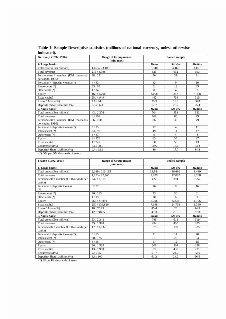
Table 1: Sample Descriptive statistics (millions of national currency, unless otherwiseindicated).Germany (1992-1996) Range of Group means

(min/ max)Pooled sample

1/ Large banks Mean Std dev MedianTotal assets (Ecu millions) 1,653 / 23,100 5,540 4,460 4,051Total revenues 218 / 3,398 825 652 593Personnel/staff number (DM thousandsper capita, 1996)

28 / 221 90 31 81

Personnel / (deposits +loans) (*) 4 / 52 12 9 10Interest cost (*) 33 / 83 51 12 49Other costs (*) 1 / 34 8 4 7Equity 160 / 2,268 433.8 357 316.8Fixed capital 25 / 4,949 482 754 315Loans / Assets (%) 7.8 / 94.6 55.5 18.3 60.8Deposits / Short liabilities (%) 0.5 / 96.4 67.7 25.7 75.42/ Small banks Mean Std dev MedianTotal assets (Ecu millions) 43 / 2,276 704 553 523Total revenues 6 / 369 109 85 79Personnel/staff number (DM thousandsper capita, 1996)

56 / 700 86 39 79

Personnel / (deposits +loans) (*) 5 / 35 12 4 11Interest cost (*) 34 / 97 49 11 47Other costs (*) 3 / 47 9 4 8Equity 4 / 576 63 56 47Fixed capital 1 / 247 60 50 43Loans/assets (%) 8.6 / 98.5 60.6 13.6 63.3Deposits/ Short liabilities (%) 0.4 / 98.9 80 17.7 84.8 (*) DM per DM thousands of assets

France (1992-1995) Range of Group means(min/ max)

Pooled sample

1/ Large banks Mean Std dev MedianTotal assets (Ecu millions) 2,189 / 210,165 13,544 36,660 3,439Total revenues 1,173 / 97,465 7,089 17,067 2,238Personnel/staff number (FF thousands percapita)

247 / 2,515 422 394 324

Personnel / (deposits +loans)(*)

1/ 27 16 8 16

Interest cost (*) 46 / 183 73 36 61Other costs (*) 1 / 19 10 6 9Equity 263 / 37,991 3,296 6,834 1,196Fixed capital 250 / 139,826 7,398 24,756 1,360Loans / Assets (%) 10 / 70.25 45.4 23 44.9Deposits / Short liabilities (%) 12.7 / 84.5 41.3 20.3 37.82/ Small banks mean Std dev MedianTotal assets (Ecu millions) 53 / 2,242 748 613 519Total revenues 35 / 1,990 494 450 355Personnel/staff number (FF thousands percapita)

178 / 1,632 375 199 325

Personnel / (deposits +loans) (*) 3 / 59 21 11 20Interest cost (*) 30 / 135 61 29 54Other costs (*) 3 / 56 17 12 15Equity 30 / 1,538 306 304 188Fixed capital 13 / 1,980 370 437 231Loans/assets (%) 2.1 / 75 51.7 21.7 52.6Deposits/ Short liabilities (%) 3.6 / 100 61.2 24.2 66.5 (*) FF per FF thousands of assets

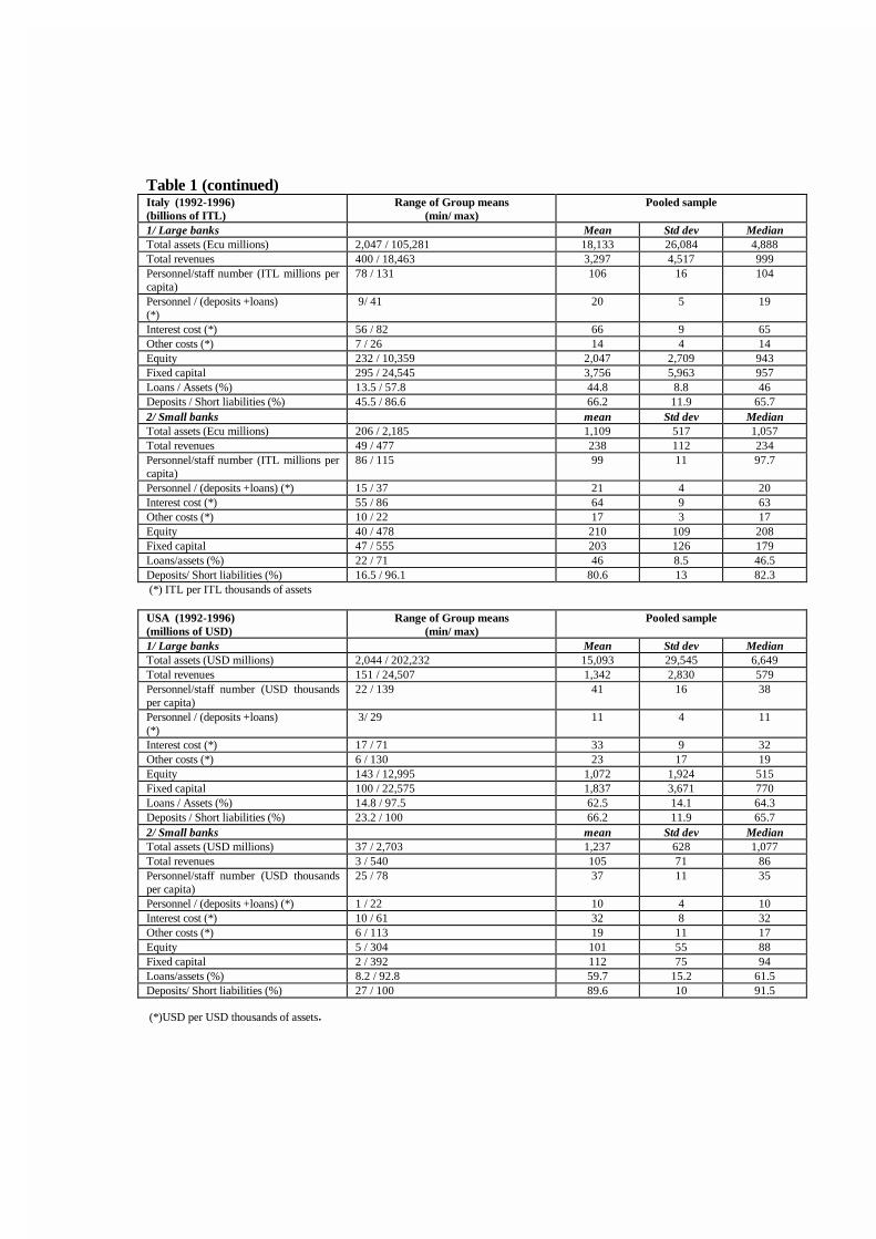
Table 1 (continued)Italy (1992-1996)(billions of ITL)

Range of Group means(min/ max)

Pooled sample

1/ Large banks Mean Std dev MedianTotal assets (Ecu millions) 2,047 / 105,281 18,133 26,084 4,888Total revenues 400 / 18,463 3,297 4,517 999Personnel/staff number (ITL millions percapita)

78 / 131 106 16 104

Personnel / (deposits +loans)(*)

9/ 41 20 5 19

Interest cost (*) 56 / 82 66 9 65Other costs (*) 7 / 26 14 4 14Equity 232 / 10,359 2,047 2,709 943Fixed capital 295 / 24,545 3,756 5,963 957Loans / Assets (%) 13.5 / 57.8 44.8 8.8 46Deposits / Short liabilities (%) 45.5 / 86.6 66.2 11.9 65.72/ Small banks mean Std dev MedianTotal assets (Ecu millions) 206 / 2,185 1,109 517 1,057Total revenues 49 / 477 238 112 234Personnel/staff number (ITL millions percapita)

86 / 115 99 11 97.7

Personnel / (deposits +loans) (*) 15 / 37 21 4 20Interest cost (*) 55 / 86 64 9 63Other costs (*) 10 / 22 17 3 17Equity 40 / 478 210 109 208Fixed capital 47 / 555 203 126 179Loans/assets (%) 22 / 71 46 8.5 46.5Deposits/ Short liabilities (%) 16.5 / 96.1 80.6 13 82.3 (*) ITL per ITL thousands of assets

USA (1992-1996)(millions of USD)

Range of Group means(min/ max)

Pooled sample

1/ Large banks Mean Std dev MedianTotal assets (USD millions) 2,044 / 202,232 15,093 29,545 6,649Total revenues 151 / 24,507 1,342 2,830 579Personnel/staff number (USD thousandsper capita)

22 / 139 41 16 38

Personnel / (deposits +loans)(*)

3/ 29 11 4 11

Interest cost (*) 17 / 71 33 9 32Other costs (*) 6 / 130 23 17 19Equity 143 / 12,995 1,072 1,924 515Fixed capital 100 / 22,575 1,837 3,671 770Loans / Assets (%) 14.8 / 97.5 62.5 14.1 64.3Deposits / Short liabilities (%) 23.2 / 100 66.2 11.9 65.72/ Small banks mean Std dev MedianTotal assets (USD millions) 37 / 2,703 1,237 628 1,077Total revenues 3 / 540 105 71 86Personnel/staff number (USD thousandsper capita)

25 / 78 37 11 35

Personnel / (deposits +loans) (*) 1 / 22 10 4 10Interest cost (*) 10 / 61 32 8 32Other costs (*) 6 / 113 19 11 17Equity 5 / 304 101 55 88Fixed capital 2 / 392 112 75 94Loans/assets (%) 8.2 / 92.8 59.7 15.2 61.5Deposits/ Short liabilities (%) 27 / 100 89.6 10 91.5

(*)USD per USD thousands of assets.

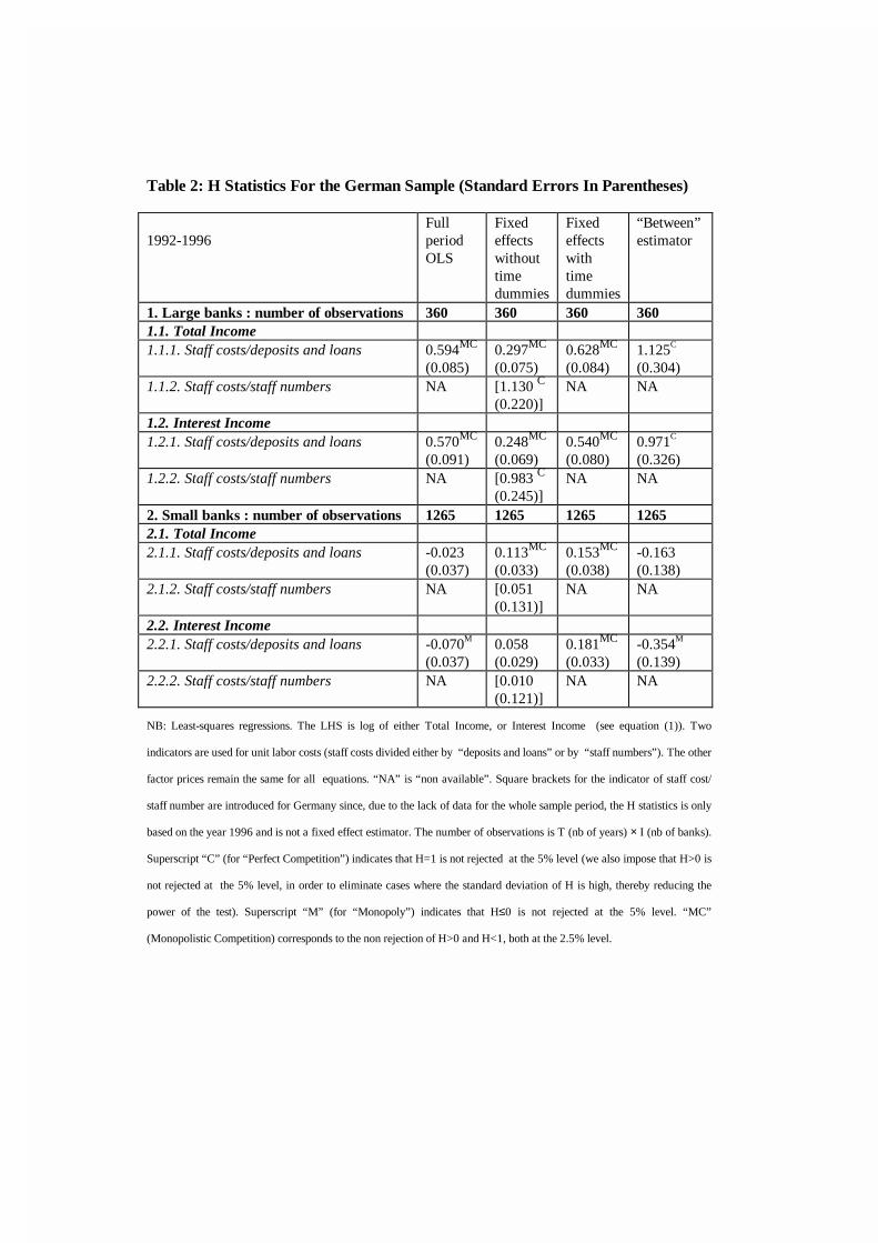
Table 2: H Statistics For the German Sample (Standard Errors In Parentheses)

1992-1996FullperiodOLS

Fixedeffectswithouttimedummies

Fixedeffectswithtimedummies

“Between”estimator

1. Large banks : number of observations 360 360 360 3601.1. Total Income1.1.1. Staff costs/deposits and loans 0.594MC

(0.085)0.297MC

(0.075)0.628MC

(0.084)1.125C

(0.304)1.1.2. Staff costs/staff numbers NA [1.130 C

(0.220)]NA NA

1.2. Interest Income1.2.1. Staff costs/deposits and loans 0.570MC

(0.091)0.248MC

(0.069)0.540MC

(0.080)0.971C

(0.326)1.2.2. Staff costs/staff numbers NA [0.983 C

(0.245)]NA NA

2. Small banks : number of observations 1265 1265 1265 12652.1. Total Income2.1.1. Staff costs/deposits and loans -0.023

(0.037)0.113MC

(0.033)0.153MC

(0.038)-0.163(0.138)

2.1.2. Staff costs/staff numbers NA [0.051(0.131)]

NA NA

2.2. Interest Income2.2.1. Staff costs/deposits and loans -0.070M

(0.037)0.058(0.029)

0.181MC

(0.033)-0.354M

(0.139)2.2.2. Staff costs/staff numbers NA [0.010

(0.121)]NA NA

NB: Least-squares regressions. The LHS is log of either Total Income, or Interest Income (see equation (1)). Two

indicators are used for unit labor costs (staff costs divided either by “deposits and loans” or by “staff numbers”). The other

factor prices remain the same for all equations. “NA” is “non available”. Square brackets for the indicator of staff cost/

staff number are introduced for Germany since, due to the lack of data for the whole sample period, the H statistics is only

based on the year 1996 and is not a fixed effect estimator. The number of observations is T (nb of years) × I (nb of banks).

Superscript “C” (for “Perfect Competition”) indicates that H=1 is not rejected at the 5% level (we also impose that H>0 is

not rejected at the 5% level, in order to eliminate cases where the standard deviation of H is high, thereby reducing the

power of the test). Superscript “M” (for “Monopoly”) indicates that H≤0 is not rejected at the 5% level. “MC”

(Monopolistic Competition) corresponds to the non rejection of H>0 and H<1, both at the 2.5% level.

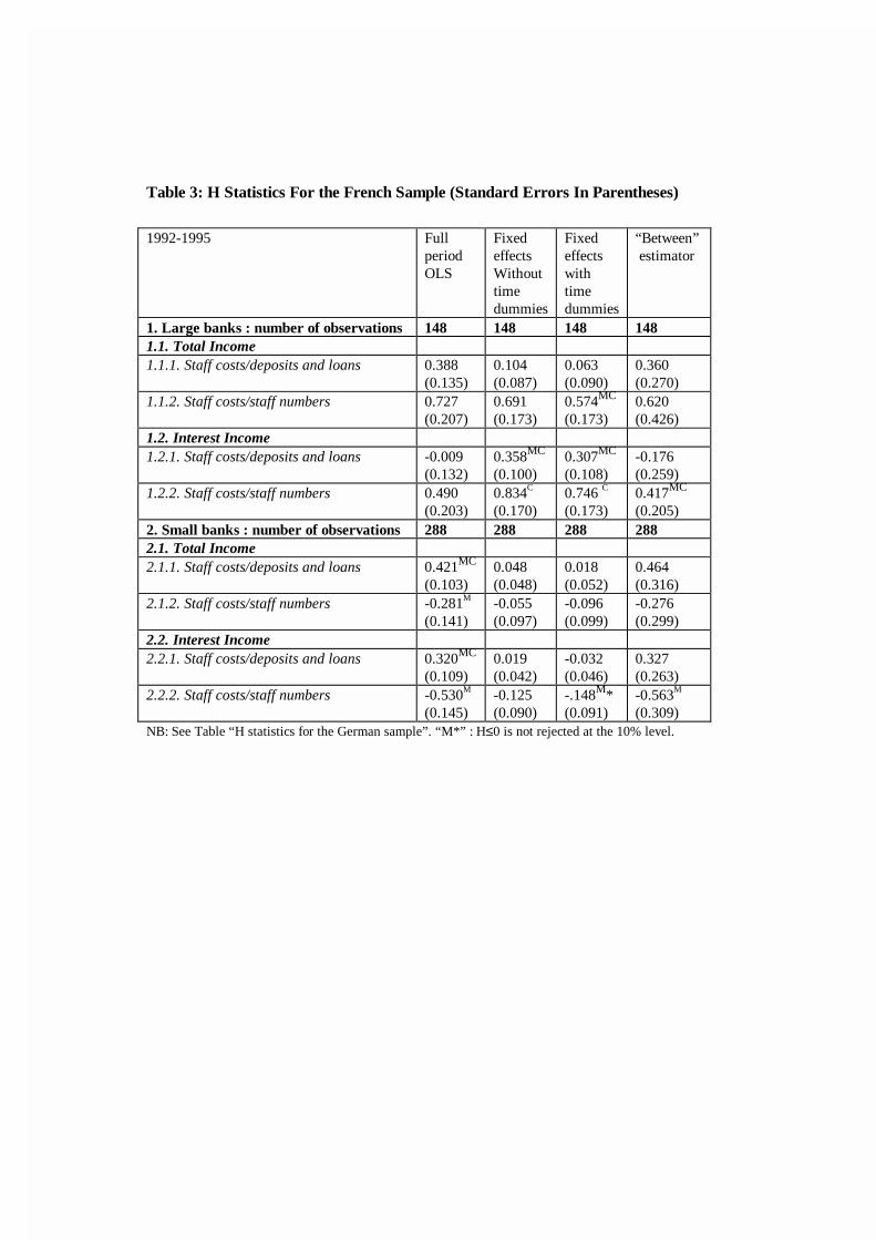
Table 3: H Statistics For the French Sample (Standard Errors In Parentheses)

1992-1995 FullperiodOLS

FixedeffectsWithouttimedummies

Fixedeffectswithtimedummies

“Between” estimator

1. Large banks : number of observations 148 148 148 1481.1. Total Income1.1.1. Staff costs/deposits and loans 0.388

(0.135)0.104(0.087)

0.063(0.090)

0.360(0.270)

1.1.2. Staff costs/staff numbers 0.727(0.207)

0.691(0.173)

0.574MC

(0.173)0.620(0.426)

1.2. Interest Income1.2.1. Staff costs/deposits and loans -0.009

(0.132)0.358MC

(0.100)0.307MC

(0.108)-0.176(0.259)

1.2.2. Staff costs/staff numbers 0.490(0.203)

0.834C

(0.170)0.746 C

(0.173)0.417MC

(0.205)2. Small banks : number of observations 288 288 288 2882.1. Total Income2.1.1. Staff costs/deposits and loans 0.421MC

(0.103)0.048(0.048)

0.018(0.052)

0.464(0.316)

2.1.2. Staff costs/staff numbers -0.281M

(0.141)-0.055(0.097)

-0.096(0.099)

-0.276(0.299)

2.2. Interest Income2.2.1. Staff costs/deposits and loans 0.320MC

(0.109)0.019(0.042)

-0.032(0.046)

0.327(0.263)

2.2.2. Staff costs/staff numbers -0.530M

(0.145)-0.125(0.090)

-.148M*(0.091)

-0.563M

(0.309)NB: See Table “H statistics for the German sample”. “M*” : H≤0 is not rejected at the 10% level.

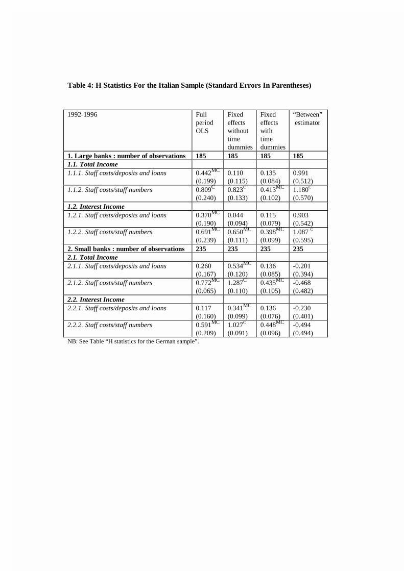
Table 4: H Statistics For the Italian Sample (Standard Errors In Parentheses)

1992-1996 FullperiodOLS

Fixedeffectswithouttimedummies

Fixedeffectswithtimedummies

“Between” estimator

1. Large banks : number of observations 185 185 185 1851.1. Total Income1.1.1. Staff costs/deposits and loans 0.442MC

(0.199)0.110(0.115)

0.135(0.084)

0.991(0.512)

1.1.2. Staff costs/staff numbers 0.809C

(0.240)0.823C

(0.133)0.413MC

(0.102)1.180C

(0.570)1.2. Interest Income1.2.1. Staff costs/deposits and loans 0.370MC

(0.190)0.044(0.094)

0.115(0.079)

0.903(0.542)

1.2.2. Staff costs/staff numbers 0.691MC

(0.239)0.650MC

(0.111)0.398MC

(0.099)1.087 C

(0.595)2. Small banks : number of observations 235 235 235 2352.1. Total Income2.1.1. Staff costs/deposits and loans 0.260

(0.167)0.534MC

(0.120)0.136(0.085)

-0.201(0.394)

2.1.2. Staff costs/staff numbers 0.772MC

(0.065)1.287C

(0.110)0.435MC

(0.105)-0.468(0.482)

2.2. Interest Income2.2.1. Staff costs/deposits and loans 0.117

(0.160)0.341MC

(0.099)0.136(0.076)

-0.230(0.401)

2.2.2. Staff costs/staff numbers 0.591MC

(0.209)1.027C

(0.091)0.448MC

(0.096)-0.494(0.494)

NB: See Table “H statistics for the German sample”.

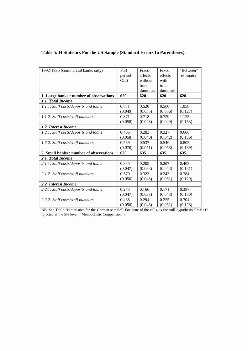
Table 5: H Statistics For the US Sample (Standard Errors In Parentheses)

1992-1996 (commercial banks only) FullperiodOLS

Fixedeffectswithouttimedummies

Fixedeffectswithtimedummies

“Between” estimator

1. Large banks : number of observations 620 620 620 6201.1. Total Income1.1.1. Staff costs/deposits and loans 0.831

(0.049)0.520(0.035)

0.560(0.036)

1.058(0.127)

1.1.2. Staff costs/staff numbers 0.871(0.058)

0.718(0.043)

0.729(0.049)

1.125(0.153)

1.2. Interest Income1.2.1. Staff costs/deposits and loans 0.486

(0.058)0.283(0.040)

0.327(0.042)

0.666(0.156)

1.2.2. Staff costs/staff numbers 0.589(0.070)

0.537(0.051)

0.546(0.058)

0.805(0.189)

2. Small banks : number of observations 635 635 635 6352.1. Total Income2.1.1. Staff costs/deposits and loans 0.335

(0.047)0.205(0.038)

0.207(0.043)

0.403(0.131)

2.1.2. Staff costs/staff numbers 0.570(0.050)

0.323(0.043)

0.243(0.051)

0.784(0.129)

2.2. Interest Income2.2.1. Staff costs/deposits and loans 0.273

(0.047)0.166(0.038)

0.171(0.043)

0.387(0.130)

2.2.2. Staff costs/staff numbers 0.468(0.050)

0.294(0.043)

0.225(0.052)

0.704(0.128)

NB: See Table “H statistics for the German sample”. For none of the cells, is the null hypothesis “0<H<1”rejected at the 5% level (“Monopolistic Competition”).

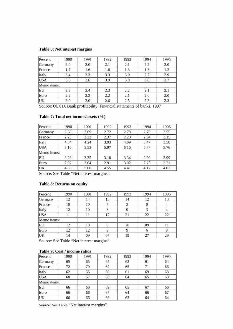
Table 6: Net interest margins

Percent 1990 1991 1992 1993 1994 1995Germany 2.0 2.0 2.1 2.1 2.2 2.0France 1.7 1.6 1.6 1.3 1.3 1.2Italy 3.4 3.3 3.3 3.0 2.7 2.9USA 3.5 3.6 3.9 3.9 3.8 3.7Memo items:EU 2.3 2.4 2.3 2.2 2.1 2.1Euro 2.2 2.3 2.2 2.1 2.0 2.0UK 3.0 3.0 2.6 2.5 2.3 2.3

Source: OECD, Bank profitability, Financial statements of banks, 1997

Table 7: Total net income/assets (%)

Percent 1990 1991 1992 1993 1994 1995Germany 2.68 2.69 2.72 2.78 2.70 2.55France 2.25 2.22 2.37 2.28 2.04 2.15Italy 4.34 4.24 3.93 4.09 3.47 3.58USA 5.16 5.53 5.97 6.16 5.77 5.76Memo items:EU 3.23 3.35 3.18 3.34 2.99 2.99Euro 2.97 3.04 2.91 3.02 2.73 2.71UK 4.83 5.00 4.55 4.41 4.12 4.07

Source: See Table “Net interest margins”.

Table 8: Returns on equity

Percent 1990 1991 1992 1993 1994 1995Germany 12 14 13 14 12 13France 10 10 7 3 0 4Italy 12 10 8 9 3 4USA 11 11 17 21 22 22Memo items:EU 12 13 8 10 09 11Euro 12 12 9 9 6 8UK 14 09 07 19 27 29

Source: See Table “Net interest margins”.

Table 9: Cost / income ratiosPercent 1990 1991 1992 1993 1994 1995Germany 65 65 65 62 61 64France 72 70 67 65 71 66Italy 62 65 66 61 69 68USA 68 67 65 64 65 63Memo items:EU 66 66 69 65 67 66Euro 66 66 67 64 66 67UK 66 66 66 63 64 64

Source: See Table “Net interest margins”.

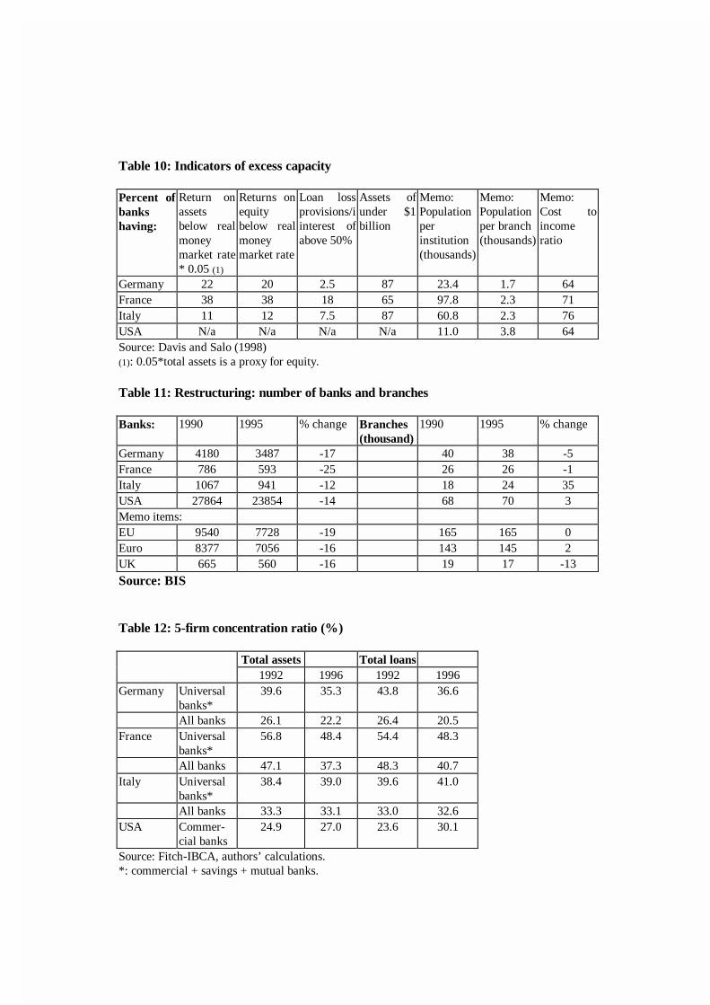
Table 10: Indicators of excess capacity

Percent ofbankshaving:

Return onassetsbelow realmoneymarket rate* 0.05 (1)

Returns onequitybelow realmoneymarket rate

Loan lossprovisions/iinterest ofabove 50%

Assets ofunder $1billion

Memo:Populationperinstitution(thousands)

Memo:Populationper branch(thousands)

Memo:Cost toincomeratio

Germany 22 20 2.5 87 23.4 1.7 64France 38 38 18 65 97.8 2.3 71Italy 11 12 7.5 87 60.8 2.3 76USA N/a N/a N/a N/a 11.0 3.8 64Source: Davis and Salo (1998)(1): 0.05*total assets is a proxy for equity.

Table 11: Restructuring: number of banks and branches

Banks: 1990 1995 % change Branches(thousand)

1990 1995 % change

Germany 4180 3487 -17 40 38 -5France 786 593 -25 26 26 -1Italy 1067 941 -12 18 24 35USA 27864 23854 -14 68 70 3Memo items:EU 9540 7728 -19 165 165 0Euro 8377 7056 -16 143 145 2UK 665 560 -16 19 17 -13

Source: BIS

Table 12: 5-firm concentration ratio (%)

Total assets Total loans1992 1996 1992 1996

Germany Universalbanks*

39.6 35.3 43.8 36.6

All banks 26.1 22.2 26.4 20.5France Universal

banks*56.8 48.4 54.4 48.3

All banks 47.1 37.3 48.3 40.7Italy Universal

banks*38.4 39.0 39.6 41.0

All banks 33.3 33.1 33.0 32.6USA Commer-

cial banks24.9 27.0 23.6 30.1

Source: Fitch-IBCA, authors’ calculations.*: commercial + savings + mutual banks.

Annex A- Definition of Variables (in logarithms, unless otherwise indicated)

1/ Endogenous variables

- Interest Revenues=Interest Received

- Total Revenues= Interest Received + Other Operating Income + Other Income

(exceptional items excluded)

- 100×Net income /Total Assets in %.

2/ Factor unit prices

- Personnel Expenses / End of Year Staff Number or Personnel Expenses / (Deposits +

Loans)

- Interest Paid / (Deposits + Other Liabilities), where Other Liabilities=Interbank Time and

Demand Deposits + Long Term Borrowing + Subordinated Debt + Participating Debt +

Hybrid Capital

- Other Non-Interest Expenses / Total Assets

3/ Capacity indicators

- Equity

- Fixed Assets + Cash and Due from Banks + Other Non Earning Assets

4/ Exogenous variables (= indicator of business mix)

- Loans / Total Assets

- Deposits / Deposits and Money Market Funding

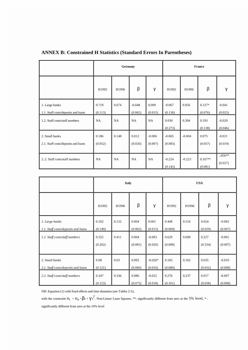
ANNEX B: Constrained H Statistics (Standard Errors In Parentheses)

Germany France

H1992 H1996 β γ H1992 H1996 β γ

1. Large banks

1.1. Staff costs/deposits and loans

0.719

(0.113)

0.674 -0.048

(0.062)

0.009

(0.015)

-0.067

(0.130)

0.056 0.127*

(0.076)

-0.041

(0.025)

1.2. Staff costs/staff numbers NA NA NA NA 0.030

(0.273)

0.394 0.193

(0.138)

-0.029

(0.046)

2. Small banks

2.1. Staff costs/deposits and loans

0.186

(0.052)

0.148 0.012

(0.026)

-0.006

(0.007)

-0.065

(0.083)

-0.004 0.075

(0.057)

-0.021

(0.019)

2..2. Staff costs/staff numbers NA NA NA NA -0.224

(0.145)

-0.223 0.167**

(0.081)

-.056**

(0.027)

Italy USA

H1992 H1996 β γ H1992 H1996 β γ

1. Large banks

1.1. Staff costs/deposits and loans

0.102

(0.149)

0.132 0.004

(0.062)

0.001

(0.015)

0.448

(0.069)

0.516 0.024

(0.029)

-0.002

(0.007)

1.2. Staff costs/staff numbers 0.352

(0.202)

0.411 0.004

(0.081)

-0.003

(0.020)

0.620

(0.088)

0.690 0.227

(0.334)

-0.001

(0.007)

2. Small banks

2.1. Staff costs/deposits and loans

0.08

(0.121)

0.03 0.092

(0.060)

-0.026*

(0.016)

0.183

(0.080)

0.162 0.035

(0.032)

-0.010

(0.008)

2.2. Staff costs/staff numbers 0.347

(0.153)

0.336 0.086

(0.073)

-0.022

(0.018)

0.276

(0.101)

0.237 0.017

(0.038)

-0.007

(0.008)

NB: Equation (1) with fixed effects and time dummies (see Tables 2-5),

with the constraint Ht = Ho +βt + γ t2

. Non-Linear Least Squares. **: significantly different from zero at the 5% level, * :

significantly different from zero at the 10% level

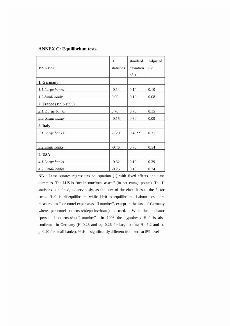
ANNEX C: Equilibrium tests

1992-1996

H

statistics

standard

deviation

of H

Adjusted

R2

1. Germany

1.1.Large banks -0.14 0.10 0.10

1.2.Small banks 0.00 0.10 0.08

2. France (1992-1995)

2.1. Large banks 0.70 0.70 0.15

2.2. Small banks -0.15 0.60 0.09

3. Italy

3.1.Large banks -1.20 0.40** 0.21

3.2.Small banks -0.46 0.70 0.14

4. USA

4.1.Large banks -0.32 0.19 0.29

4.2. Small banks -0.26 0.18 0.74

NB : Least squares regressions on equation (1) with fixed effects and time

dummies. The LHS is “net income/total assets” (in percentage points). The H

statistics is defined, as previously, as the sum of the elasticities to the factor

costs. H<0 is disequilibrium while H=0 is equilibrium. Labour costs are

measured as “personnel expenses/staff number”, except in the case of Germany

where personnel expenses/(deposits+loans) is used. With the indicator

“personnel expenses/staff number” in 1996 the hypothesis H=0 is also

confirmed in Germany (H=0.26 and σH=0.26 for large banks; H=-1.2 and σ

H=0.20 for small banks). **:H is significantly different from zero at 5% level

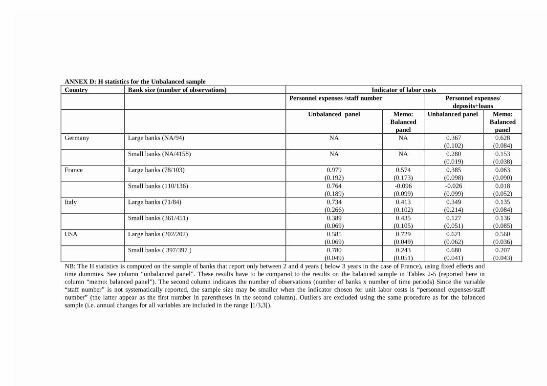
ANNEX D: H statistics for the Unbalanced sampleCountry Bank size (number of observations) Indicator of labor costs

Personnel expenses /staff number Personnel expenses/deposits+loans

Unbalanced panel Memo:Balanced

panel

Unbalanced panel Memo:Balanced

panelGermany Large banks (NA/94) NA NA 0.367

(0.102)0.628

(0.084)Small banks (NA/4158) NA NA 0.280

(0.019)0.153

(0.038)France Large banks (78/103) 0.979

(0.192)0.574

(0.173)0.385

(0.098)0.063

(0.090)Small banks (110/136) 0.764

(0.189)-0.096(0.099)

-0.026(0.099)

0.018(0.052)

Italy Large banks (71/84) 0.734(0.266)

0.413(0.102)

0.349(0.214)

0.135(0.084)

Small banks (361/451) 0.389(0.069)

0.435(0.105)

0.127(0.051)

0.136(0.085)

USA Large banks (202/202) 0.585(0.069)

0.729(0.049)

0.621(0.062)

0.560(0.036)

Small banks ( 397/397 ) 0.780(0.049)

0.243(0.051)

0.680(0.041)

0.207(0.043)

NB: The H statistics is computed on the sample of banks that report only between 2 and 4 years ( below 3 years in the case of France), using fixed effects andtime dummies. See column “unbalanced panel”. These results have to be compared to the results on the balanced sample in Tables 2-5 (reported here incolumn “memo: balanced panel”). The second column indicates the number of observations (number of banks x number of time periods) Since the variable“staff number” is not systematically reported, the sample size may be smaller when the indicator chosen for unit labor costs is “personnel expenses/staffnumber” (the latter appear as the first number in parentheses in the second column). Outliers are excluded using the same procedure as for the balancedsample (i.e. annual changes for all variables are included in the range ]1/3,3[).

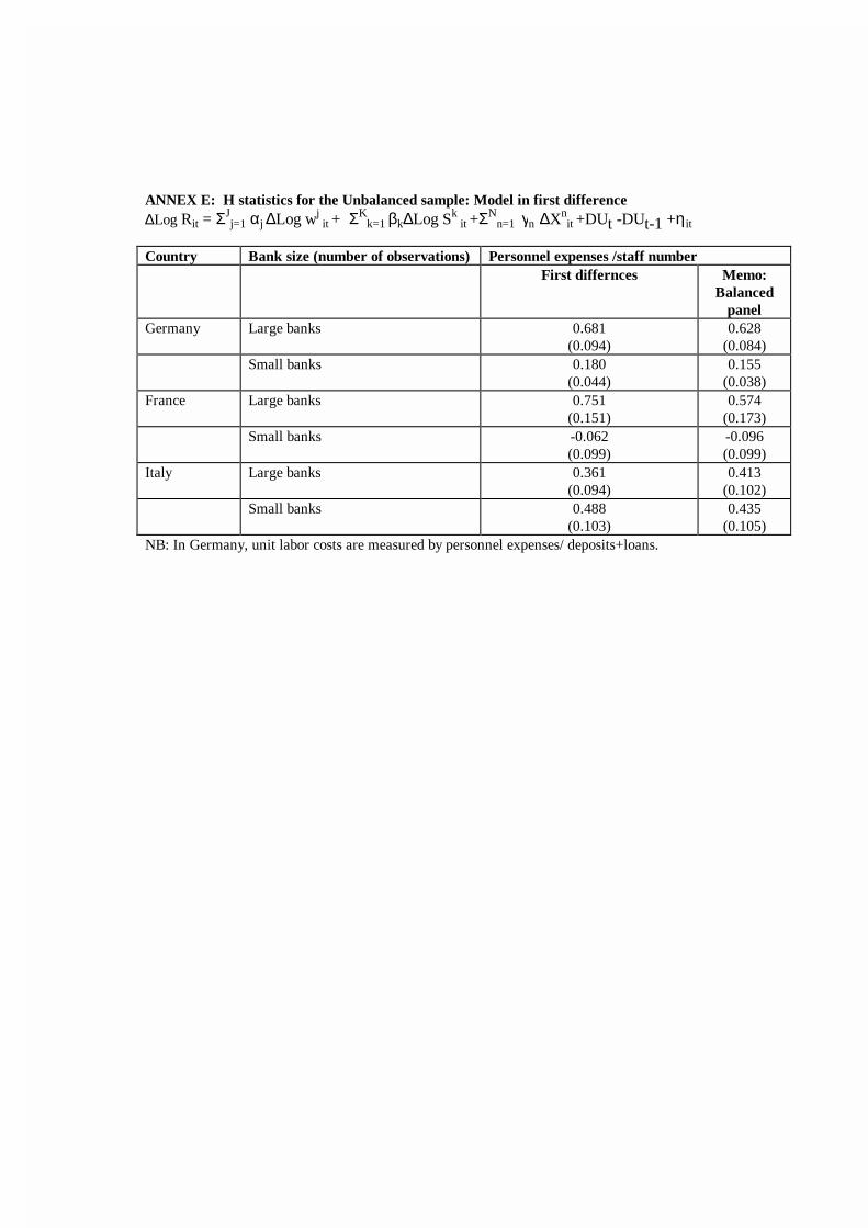
ANNEX E: H statistics for the Unbalanced sample: Model in first difference∆Log Rit = ΣJ

j=1 αj ∆Log wj it + ΣK

k=1 βk∆Log Sk it +ΣN

n=1 γn ∆Xnit +DUt -DUt-1 +ηit

Country Bank size (number of observations) Personnel expenses /staff numberFirst differnces Memo:

Balancedpanel

Germany Large banks 0.681(0.094)

0.628(0.084)

Small banks 0.180(0.044)

0.155(0.038)

France Large banks 0.751(0.151)

0.574(0.173)

Small banks -0.062(0.099)

-0.096(0.099)

Italy Large banks 0.361(0.094)

0.413(0.102)

Small banks 0.488(0.103)

0.435(0.105)

NB: In Germany, unit labor costs are measured by personnel expenses/ deposits+loans.

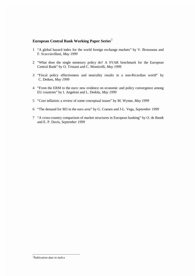
European Central Bank Working Paper Series∗

1 “A global hazard index for the world foreign exchange markets” by V. Brousseau andF. Scacciavillani, May 1999

2 “What does the single monetary policy do? A SVAR benchmark for the EuropeanCentral Bank” by O. Tristani and C. Monticelli, May 1999

3 “Fiscal policy effectiveness and neutrality results in a non-Ricardian world” byC. Detken, May 1999

4 “From the ERM to the euro: new evidence on economic and policy convergence amongEU countries” by I. Angeloni and L. Dedola, May 1999

5 “Core inflation: a review of some conceptual issues” by M. Wynne, May 1999

6 “The demand for M3 in the euro area” by G. Coenen and J-L. Vega, September 1999

7 “A cross-country comparison of market structures in European banking” by O. de Bandtand E. P. Davis, September 1999

∗ Publication date in italics