* For Correspondence: College of Business, FM 1098 & University Dr., Prairie View, TX 77002. Phone: (936)261-9223. Email: chsheh@pvamu.edu. We thank Praveen Kumar, Tom George, and Craig Pirrong for helpful comments and suggestions. The views expressed herein are solely those of the authors and not those of any other person or entity. Any errors are ours alone.

Dealer Competition and Financial Market Performance:

An Experimental Analysis Between Monopoly and Duopoly Structures

By

Chi Sheh*

College of Business, Prairie View A&M University

Nathaniel Wilcox

Economic Science Institute, Chapman University and

Department of Economics, University of Houston

December 12, 2009

Dealer Competition and Financial Market Performance:

An Experimental Analysis Between Monopoly and Duopoly Structures

Abstract

The question of whether a monopolist market maker can support a more resilient dealer

market than competing market makers under asymmetric information remains unresolved

despite several empirical studies of extensive financial market data. We examine the

effects of dealer competition and asymmetric information in a continuous multiple-dealer

experimental market in which human subjects trade a single security. We find that

contrary to extant theory, a duopoly market structure is more resilient than a monopoly

market structure under a severe asymmetric information environment. We find evidence

of stochastic maximization in both markets while loss and risk aversion are significant

factors in explaining monopolist behavior.

JEL classification: G24, D82, C90, D42

Key words: Dealer Market; Competition; Market Structure; Market Experiments

1

I. INTRODUCTION

The last decade has seen a wave of consolidation and reorganization of financial exchanges around the world. In light of the biggest financial crisis of a generation, the search for better and more resilient market mechanisms is of crucial concern. What we term resilient markets are market structures that will not break down even in environments where asymmetric information is rampant.

In an era of electronic and automated trading mechanisms, is there a role for dealers and specifically a monopolist specialist? This issue has important implications both with respect to the search for better market designs and broader issues concerning the industrial organization of financial markets, which is of interest to both academics and regulators alike.

This paper contributes to the existing market microstructure literature by examining the effects of dealer competition and asymmetric information on the financial performance of the dealer market institution. Specifically, we seek to find out whether in fact a monopolist specialist can produce a more resilient market than competing duopolist market makers under asymmetric information.

Glosten, in his seminal paper “Insider Trading, Liquidity, and the Role of the Monopolist Specialist” (The Journal of Business, 1989), provides a theoretical rationale for the existence of the monopolist dealer known as the specialist. He shows that in environments where the asymmetric information problem is severe, a monopolist specialist will keep the market open while competing market makers would shut the market down. The result is that a monopolist is predicted to provide a more liquid market in environments with severe asymmetric information. We term this result the “Glosten result”. It is this prediction that we wish to test with an experimental design which compares the resiliency of the monopoly vs. the competitive (duopoly) market structure.

The experimental method is ideally suited for this investigation for three main reasons. First, while information asymmetry plays a substantial role in many market microstructure models, it is difficult to evaluate its presence or estimate its severity in naturally occurring (field) data. Different empirical studies use different proxies for level of asymmetric information.1

1 For an overview and comparison of the diverse information asymmetry metrics used in market microstructure and

corporate finance, see Clarke and Shastri (2000)

The use of different proxies makes the comparison of their results difficult, as well as creating ambiguity in terms of whether the environment examined really has a high level of asymmetric information. In a controlled experiment, the level and exact specification of the information asymmetry can be established exogenously, allowing for a clear assessment of its impact on trading, pricing, and market efficiency. Second, a direct comparison of different market structures, like a monopoly and a duopoly, in a financial market for the same security is very difficult using standard field data. Many securities either have a monopolist specialist or have competing market makers, but there are very few securities that trade under both market

2

mechanisms. Even when found, differences in regulatory constraints make direct comparisons difficult without imposing untestable identifying restrictions. Third, the severe asymmetric information environments which are the focus of this investigation may be rare, which compounds the problem of finding suitable field data.

The rest of the study is organized as follows. We conduct a literature review in the Section II, in which previous theoretical and empirical studies related to the financial performance of diverse market structures under asymmetric information are examined. In Section III, we present the experimental design that details the procedures, subjects, and environment used in this study. Using a classical Mixed Strategy Nash Equilibrium (MSNE) framework, the development of testable hypotheses is presented in section IV. Section V presents a detailed analysis of the results of the experiment. We also show how a quantal response equilibrium (QRE) model specification can be used to explain some of the key experimental results. Section VI presents concluding remarks and possible avenues of future research.

II. LITERATURE REVIEW

A. Theoretical Background There have been several theoretical studies that make predictions with respect to the impact of competition on dealer markets. Ho and Stoll (1983) present a dynamic programming model where dealers post differential bid-ask quotes due to prior inventory and risk attitude differences. They predict bid-ask spread to be lower as the number of dealers rises. Dennert (1993) shows that if market makers have to commit themselves before observing the actual order flow, a higher number of market makers will induce higher transaction costs for the liquidity traders2, since the risk exposure of the individual market maker increases. In his model, the market maker’s exposure to insider3

2 Liquidity traders are also termed “uninformed traders” and/or “noise traders” in related literature. In this study, we

adopt a widely held notion in market microstructure literature specifying liquidity traders as those traders that carry

out “liquidity motivated” trade, or trade unrelated to information. A rationale for this type of trading can be found in

Grossman and Miller (1988), where the authors refer to liquidity traders as “outside customers who, for any of a

variety of reasons, experience a liquidity event, which leads them to perceive a gap at current prices between their

desired holdings of a particular asset and their current holdings of an asset. “

risk grows with the number of competitors and therefore she will in equilibrium demand a higher bid-ask spread.

3 Insiders are commonly referred to as “informed traders” (Glosten and Milgrom (1985), Kyle (1985)). We use the

theoretical convention that informed traders (insiders) have unique access to the private information of the

liquidation value of the traded risky asset.

3

More modern treatments of dealer markets inject strategic behavior to market makers in the provision of liquidity under asymmetric information. Biais, Martimort, and Rochet (2000) model strategic liquidity suppliers (dealers) posting non-linear price schedules at which they stand ready to trade with a risk-averse agent. Their model predicts that competition among market makers leads to a deeper market, since the overall volume increases and the spread decreases with a higher number of market makers. Bondarenko (2001) predicts in his model that when the number of market makers increases, each market maker handles a smaller order flow, and the residual demand faced by each market maker becomes more elastic. Therefore, the expected profits of each individual market maker as well as of the whole group decrease. A more recent study by Germain and Rousseau (2005) sets up a model with risk averse market makers and risk averse traders, along with information asymmetry and order splitting. Their model predicts that risk aversion reduces competition between market makers as it acts as a commitment for market makers to set higher prices. In their study, when market makers are risk averse, overall trader’s cost of trading may be increasing with the number of market makers. The question of whether there is a role for a monopolist specialist is a question that has been tackled by some prominent theorists. Glosten (1989) finds that while competing market makers will expect a zero profit on every trade, a monopoly specialist can average profits over trades, profiting from uninformed traders while suffering losses against informed traders. He predicts that in environments where the adverse selection problem is too extreme, competing market maker markets may shut down while a profit maximizing specialist may decide to keep the market open.4

Not surprisingly, as the predictions of these theoretical studies show, different assumptions about the underlying market structure and/or environment leads to different model predictions. Our study derives its biggest inspiration from the ideas and predictions presented in the Glosten (1989) and Grossman and Miller (1988) studies. Our goal of creating a robust test to their monopolist predictions lead to the experimental design presented in the next section.

Therefore, a specialist market will have greater liquidity under moderate or severe adverse selection. The intuition behind this “Glosten result” is that a monopolist specialist may suffer losses with informed agents, but these trades provide him with information that he can exploit in trades with liquidity traders. Grossman and Miller (1988) find that quoted bid-ask spreads and market maker’s profits will be driven towards zero by the competitive entry of new market makers. In their view, since “fixed costs are large relative to the entry-inhibiting trading risks, a competitive market may not be viable because the market makers would have no way of recovering their fixed costs of maintaining a presence on the floor.” (p. 629).

4 Bhattacharya and Spiegel (1991) examine market breakdowns in a model where dealers can employ nonlinear

strategy functions; Glosten (1989) examines linear price schedules.

4

B. Empirical Evidence Empirical studies on the impact of competition on dealer markets document important differences between the specialist and competitive market maker structures. Klock and McCormick (1999) use monthly database on 5,288 Nasdaq securities over 8 years and find that the number of market makers (dealers) has a negative and highly significant impact on bid-ask spreads. They estimate that each additional market maker will decrease the market bid-ask spread approximately $0.15 on a $20 stock (t-stat = 107). Their study manages to control for endogeneity5

Neal (1992) uses a more refined approach that exploits the historical options “allocations plan” to resolve identification problems that normally plague these comparison studies. As he points out, it is hard to distinguish between transaction cost differentials due to market structure from those due to the characteristics of the underlying asset. By exploiting the regulatory barrier imposed by the “allocations plan”, he examines a sample of 26 AMEX (specialist market) and 15 CBOE (competitive marker maker market) near-term, at the money call options from January to April 1986. His results show that when trading volume is low, the specialist structure has lower bid-ask spreads than competitive market maker structure. Interestingly, his results also suggest that as volume rises, the difference appears to diminish.

of the number of market makers by using instrumental variables. Their results suggest that the number of market makers can be affected by the size of the spread as well as vice versa. In support of these results, Ellis, Michaely, and O’Hara (2002) sample 313 firms that went public on the Nasdaq from September 1996 to July 1997 (with a focus on IPO stocks), and find that spreads decrease as the number of market makers increase. They also examine the effect of market concentration and find that spreads increase as market concentration increases.

There is a dearth of empirical studies that directly study the question on whether specialist markets provide more resilient services than competitive dealer markets. The closest study to this question we could find was by Chung and Kim (2008), who sample 1,924 NYSE stocks and 1,524 NASDAQ stocks and obtain their trade and quote data from November 1997 to December 2003 to examine their relative resiliency. Their results suggest that the NYSE specialist system provides better liquidity services than NASDAQ dealer system in times of high uncertainty, particularly for risky stocks. They also find evidence that both NASDAQ and NYSE spreads are larger in times of higher volatility. Whether the times of high return volatility correspond directly to the times where there is more adverse selection risk6

5 The reason why there is an endogeneity problem is because NASDAQ market makers may enter and drop out at

will. As a consequence, the number of market makers, according to Klock and McCormick (1999), should be

affected by the size of the bid-ask spread and vice versa.

, as the authors maintain, is perhaps subject to debate.

6 Heidle and Huang (2002) assert that Nasdaq is less able to discern informed traders from uninformed traders by

finding their probability of informed trading to be higher than NYSE and AMEX.

5

There is an important point that needs clarification in terms of how the word ‘resiliency’ is used in the Chung and Kim (2008) versus the way we view market resiliency in this study. We use the word resilient in referring to a market that is open (dealer posts quotes) versus a market that is closed (dealer(s) don’t post quotes) when subjected to asymmetric information. Chung and Kim (2008) uses resiliency as a synonym of “better liquidity services”, which in their study means tighter bid-ask spreads. This is an important distinction, since in our view, the concept of resiliency connects directly to the economist’s notion of market efficiency. In an asset market with expected value maximizers, the bid-ask spread determines the distributive issue of who gets the surplus. We believe that the concept of market resilience should be framed in terms of “how often is the market open for trade” as this provides a clear linkage to market efficiency. The reason for this is that when markets are not open, liquidity traders cannot execute surplus-enhancing trades (even in expected value terms).

C. Experimental Studies One of the first studies that took advantage of the experimental methodology in the analysis of a key feature of dealer market structure was by Flood, Huisman, Koedijk, and Mahieu (1999), where they examine the effects of price disclosure7 under transparent vs. opaque quoting environments. Their experiment uses seven professional market makers playing the role of dealers trading with one another and with computerized informed and liquidity traders. Their experimental environment was set up as a continuous, multiple dealer version of the Glosten and Milgrom (1985) model, which is a quote driven model. Similar to the experimental design that we use in our experiment8

A more recent experimental study that sheds light on how competition affects dealer markets was carried out by Krahnen and Weber (2001). They find that competition among market makers (4 dealers vs. 1 dealer) significantly reduces the bid-ask spread, and increases the

, dealers both set quotes to trade and are confronted with informed and liquidity motivated investors who view the quoted bid and ask and decide whether to trade or not. They find that spreads are wider and volume is lower in opaque markets but price discovery is much faster in opaque markets, yielding an interesting insight in the design of markets by analyzing the trade offs associated with transparency. A disconcerting fact in this study that stands out is that average market maker profits are negative in every round, calling into question the sustainability of these markets.

7 The way in which the transparent and opaque markets differ in Flood et al. (1999) is as follows: The transparent

market, all quotes are disclosed publicly and immediately, which means that all market makers have all outstanding

quotes presented on their private trading screens. In the opaque market, no quotes are publicly disclosed, and the

market maker must call one another for price quotes. 8 The experiment carried out in this study is not performed under a continuous trading environment and it also does

not allow subjects to initiate trades on their own account. There is significant interdealer trading in Flood et al.

(1999)

6

transaction volume. Their experimental results indicates that competition induces competitive undercutting, yielding net trading losses for market markers as a group. Their study raises an interesting question with respect to optimal security market design. While uninformed traders find competitive market optimal, since it minimizes their expected trading losses, dealer profits are negative on average for the 4 dealer markets. They key common finding in these two experiments that motivate our experimental design is the fact that when the number of competitors is exogenously set to be greater than 1 (non-monopoly), profits are systematically negative. Both of these experimental designs “force” the dealer to participate in the market (since the subjects are only paid based on their trading profits within the markets). In our experiment, entry is endogenous, and the choice of entry is not “forced” upon the subjects since they have the choice to “opt-out” and enjoy a salient benefit (opt-out fee) from their inaction. This feature of endogenous entry is, to our knowledge, a unique feature that has not been applied in any other experimental study of dealer markets. In the broader framework of competitive markets, the (socially) optimal situation is one where trade is always possible for liquidity traders. This leads to our central question: What market structure leads to the highest liquidity, that is, the largest fraction of trading periods in which the liquidity traders can execute trades? We intend to shed some light on this question by studying the issue of dealer market resiliency in the face of severe asymmetric information for monopoly and duopoly dealer structures.

III. EXPERIMENTAL DESIGN, SUBJECTS, AND PROCEDURES In order to provide a clear connection between the testable hypotheses presented in the next section and the experiments that were used to test them, we have chosen to present the specific details of the experimental design and environment here first. This will make the exact details of the game played by dealers in the experiment very concrete. Then, Section IV will theoretically analyze this game and derive theoretical predictions for the experiment.

As presented in the previous section, the two main theoretical studies (Glosten 1989, Grossman and Stiglitz 1988) that inspired our work here provide us guidelines as to the important elements that may impact market resiliency in dealer markets. While useful, their theoretical models are too broad in scope to be tested directly using the experimental methodology. The experimental games described in this section borrow key features from these two broader theoretical papers to produce a relatively simple pair of games—one a monopoly dealer game and the other a duopoly dealer game—that can together test an emergent “Glosten result.”

The next section will derive the relevant hypotheses for this test for the specific monopoly and duopoly games described in detail in this section. In order to both fully appreciate the richness as well as the limitations of this model, which was created subject to pragmatic experimental constraints (human, technical, financial, and methodological), we believe the reader

7

is best served by first understanding the details of our experimental environments, and then proceeding to the theoretical analysis later.

A. Experimental Design

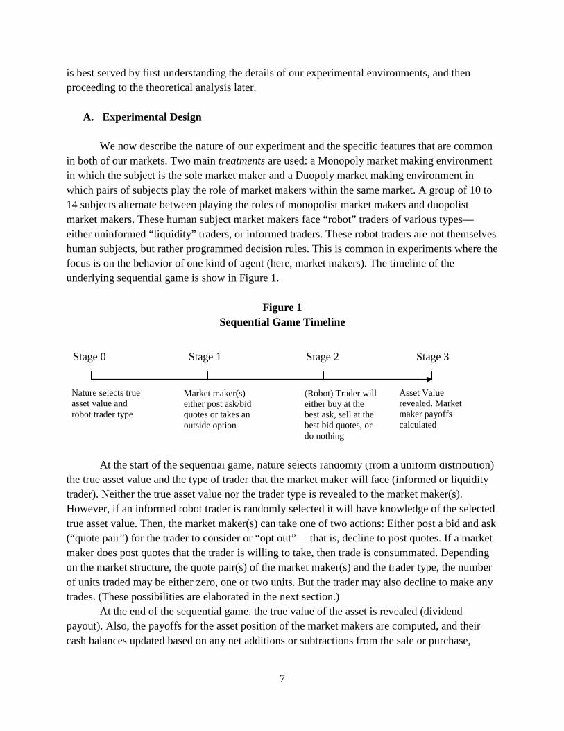
We now describe the nature of our experiment and the specific features that are common in both of our markets. Two main treatments are used: a Monopoly market making environment in which the subject is the sole market maker and a Duopoly market making environment in which pairs of subjects play the role of market makers within the same market. A group of 10 to 14 subjects alternate between playing the roles of monopolist market makers and duopolist market makers. These human subject market makers face “robot” traders of various types—either uninformed “liquidity” traders, or informed traders. These robot traders are not themselves human subjects, but rather programmed decision rules. This is common in experiments where the focus is on the behavior of one kind of agent (here, market makers). The timeline of the underlying sequential game is show in Figure 1.

Figure 1

Sequential Game Timeline

At the start of the sequential game, nature selects randomly (from a uniform distribution) the true asset value and the type of trader that the market maker will face (informed or liquidity trader). Neither the true asset value nor the trader type is revealed to the market maker(s). However, if an informed robot trader is randomly selected it will have knowledge of the selected true asset value. Then, the market maker(s) can take one of two actions: Either post a bid and ask (“quote pair”) for the trader to consider or “opt out”— that is, decline to post quotes. If a market maker does post quotes that the trader is willing to take, then trade is consummated. Depending on the market structure, the quote pair(s) of the market maker(s) and the trader type, the number of units traded may be either zero, one or two units. But the trader may also decline to make any trades. (These possibilities are elaborated in the next section.)

At the end of the sequential game, the true value of the asset is revealed (dividend payout). Also, the payoffs for the asset position of the market makers are computed, and their cash balances updated based on any net additions or subtractions from the sale or purchase,

Stage 1 Stage 0 Stage 2 Stage 3

Nature selects true asset value and robot trader type

Market maker(s) either post ask/bid quotes or takes an outside option

(Robot) Trader will either buy at the best ask, sell at the best bid quotes, or do nothing

Asset Value revealed. Market maker payoffs calculated

8

respectively, of assets. If a market maker “opts-out” (decline to post quotes), she instead receives an “outside option” with payoff f > 0 , which is added to her cash balance.

The conceptual interpretation of the outside option, which we call the “opt-out” strategy, represents a fixed cost associated with making a market—both the opportunity costs as well as the direct and indirect costs of communicating bid/ask quotes. The theoretical basis for the presence of such fixed costs (and hence the presence of the opt-out strategy in the experiment) can be found in Grossman and Miller9

In this experiment, opting out has a sure payoff of f = 1.8 in the payoff matrix (which may be thought as a fixed cost of doing business in each period). One of the reasons for this framework is to encourage subjects to view posting quotes and opting out on an equal footing. Both strategies are valid choices for subjects to earn cash, and presenting it this way meant to decrease the likelihood that they will think the experimenter wants them to post quotes. An alternative would be to endow subjects with extra cash equal to 1.8 and tell them that this must be paid in order to post quotes. But then the subjects might treat such an out-of-pocket payment as a loss, and value it differently from profits, for reasons suggested by prospect theory (Kahneman and Tversky 1979). Framing this cost as a foregone outside option prevents this unwanted effect (e.g. as in Van Boening and Wilcox 1996).

(The Journal of Finance, 1988), where such fixed costs play a crucial theoretical role. In the actual experimental setup, this opt-out fee will be framed as a foregone opportunity and not a direct cost.

B. Market Treatments

There are two main treatments in this experiment, a monopoly market and a duopoly

market. For both treatments, market makers move first, either opting out or submitting an ask and bid quote pair (a,b), where 11 > a ≥ E(vt) ≥ b > 1, which are binding proposals for a contract price: a is a selling price or ask, and b is a buying price or bid. In the monopoly case, there is obviously just one market maker. In duopoly there are two, and it results in a Bertrand pricing game. Both market makers submit their ask/bid quote pairs simultaneously without knowledge of each others’ choices. For monopolists, the ask/bid pair is denoted (am,bm); for duopolists 1 and 2, we denote their ask/bid pairs as (a1,b1) and (a2,b2), respectively. We also define the quote pair (a*,b*) as follows:

a) In the Monopoly, (a*,b*) ≡ (am,bm) b) In the Duopoly, (a*,b*) ≡ (min[a1,a2],max[b1,b2]). This is basically the market ask/bid, and (a*− b* ) is the market bid/ask spread.

9 George, Kaul, and Nimalendran (1994) show that transaction costs can affect the adverse selection problem in a

specialist market in an indirect and ambiguous way, casting doubt on the use of trading volume as an indicator of

asymmetric information.

9

C. A “Glosten” Design

In our “Glosten” model, vh = 10 correspond to the reservation price for the Liquidity Buyer and vl = 2 correspond to the reservation price for the Liquidity Seller. If ψ = 0.5 (probability of trading with an informed trader =50%), and there is an equal chance for the liquidity trader to be a buyer or seller, then there is a 25% chance of the liquidity trader to be a buyer or seller.

The level of asymmetric information ψ is specified by the probability of the market maker facing an informed trader (ψ = 0.5). This level is kept constant across all treatments, sessions, and periods to provide a clear test of the impact of competition on the rate of market closure. This level of asymmetric information is meant to represent an environment where asymmetric information problems are severe.

Figure 2 Robot Trader Decision Tree

Robot Trader

θ

Informed Trader

Liquidity Trader

½

½

Buy Market Order ( If lowest Ask ≤ 10 )

Sell Market Order ( If highest Bid ≥ 2)

Buy Market Order ( If lowest Ask < vt )

Sell Market Order ( If highest Bid > vt )

½

½

Do Nothing ( If lowest Ask ≥ vt and highest Bid ≤ vt )

Liquidity Buyer

Liquidity Seller

Do Nothing ( If lowest Ask > 10 )

Do Nothing ( If highest Bid < 2 )

10

D. Trader Types

Before the start of each period, a single “robot” trader of type θ (see Figure 2), who is interested in buying or selling two units of the asset, is randomly selected from a distribution of three possible robot trader types. (Informed, Liquidity Buyer, Liquidity Seller) The market includes two types of agents, (human) market makers, who both are able to post bid and ask quotes, and a (robot) trader that can only submit market orders.

Human subjects only play the role of market makers. They can only post bid and ask quotes and cannot submit market orders. The robot trader represents an external customer of the exchange and serves the role of either an informed trader or a liquidity buyer/seller. This is accomplished by using three computerized decision rules, representing the three possible “robots”.

The informed trader knows something that neither the liquidity traders, nor the human subjects, know: The true vt payoff of the asset for the trading period. It optimally exploits this privileged “insider” knowledge to maximize its own trading profits. It will buy two shares of the asset at the best ask quote if the dividend payoff of the share is higher than the ask price, and it will sell two shares of the asset at the best bid quote if the vt payoff of the share is lower than the bid price.

The liquidity buyer (seller), on the other hand, will buy (sell) two shares of the asset from (to) the market maker with the best ask (bid) quote, provided it is consistent with her reservation price (see Figure 2). Human market makers know the three possible decision rules of the trader. They also know the probability distributions over these three trader types, but they do not know which type of trader has actually been “drawn by nature” when they choose their strategies in each period.

The rationale behind the employment of robot traders is twofold: First, it removes strategic uncertainty about the behavior of traders (though not about trader type), and second, it increases statistical power by reducing the number of human subjects required to create observations, decreasing the cost of each observation and increasing statistical power, given a fixed experimental budget.

E. Order Splitting and Tie-breaking in Duopoly Markets

The reason why a two share endowment was chosen instead of a one share endowment is because of the possibility of ties in the Duopoly market. Unlike the Monopoly market, which obviously cannot produce any ties since there is only one dealer, the Duopoly market presents the difficulty of what to do when both dealers quote the exact same Bid, Ask, or both. In order to address this issue, we chose to endow the dealers with two shares in both markets, and to set the order size of traders at two units as well. This allows for the dealers in the Duopoly market in particular to share equally in the asset purchase (sale) when bid (ask) quote ties do occur. The

11

robot traders are programmed to split their two unit order (buy or sell) between the two duopolists when faced with a tie in dealer quotes in the Duopoly market.

F. Treatment Design

A run consists of T repeated sequential stage games, indexed by t = 1, 2, …, T (40 for Monopoly and 80 for Duopoly) periods. To discourage subjects from applying multi-period dynamic strategies when playing the duopolist roles, a random rematching protocol is used for the duopoly treatments in the experiment. This means that after playing each stage game t, each duopolist is randomly rematched to a new duopolist opponent to the next stage game t+1. This will allow subjects to learn about stage game play while discouraging them from engaging in pointless dynamic strategies.

A session begins with instructions and practice periods with somewhat different characteristics from the runs that follow (this is described below).. Then each session proceeds with two treatment runs: A monopoly run with T = 40 periods and a duopoly run with T = 80 periods. Three sessions in total were conducted in this experiment.

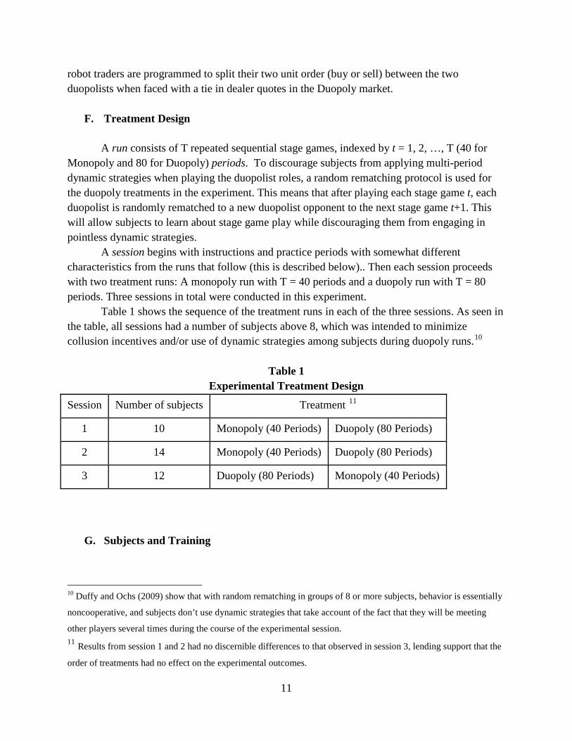
Table 1 shows the sequence of the treatment runs in each of the three sessions. As seen in the table, all sessions had a number of subjects above 8, which was intended to minimize collusion incentives and/or use of dynamic strategies among subjects during duopoly runs.10

Table 1 Experimental Treatment Design

Session Number of subjects Treatment 11

1 10 Monopoly (40 Periods) Duopoly (80 Periods)

2 14 Monopoly (40 Periods) Duopoly (80 Periods)

3 12 Duopoly (80 Periods) Monopoly (40 Periods)

G. Subjects and Training

10 Duffy and Ochs (2009) show that with random rematching in groups of 8 or more subjects, behavior is essentially

noncooperative, and subjects don’t use dynamic strategies that take account of the fact that they will be meeting

other players several times during the course of the experimental session. 11 Results from session 1 and 2 had no discernible differences to that observed in session 3, lending support that the

order of treatments had no effect on the experimental outcomes.

12

The experiments were carried out in the AIM Center at the C.T. Bauer College of Business at the University of Houston. Each subject received a handout containing experimental instructions12

Subjects also were guided through a sequence of practice trading periods, designed to ensure a clear understanding of the trading environment as well as the differences between the monopoly and duopoly treatments. The administrator then guided subjects through the use and interpretation of the computer interface by a series of practice periods, which mimicked the actual experiment, except that the trading outcomes did not affect the subject’s cash payouts.

as well as a tutorial on how to use the computer terminal. During the tutorial, experimental instructions were read, and the subjects became acquainted with the terminology used in the.

In the practice trading periods conducted during the tutorial, the identity of the (robot) trader faced by the subject was revealed at the end of each training period to facilitate learning of the game. In the actual treatment runs that followed, the identity of the (robot) trader is hidden and never directly revealed to simulate the task faced by market makers in real markets. Of course, as is the case with real-world dealers, subject dealers can frequently make inferences about the kind of trader they have just dealt with from that trader’s behavior.

After the conclusion of instruction and practice, and before the start of the treatment runs, the administrator in addition reiterated the parameter values for the asset, and reminded the subjects of the distribution of trader types and the fact that a new trader type would be drawn from this distribution at the start of each and every stage game in the treatment runs

H. Incentives

Cash winnings for each subject were determined by aggregating the L$ balances across all periods for each subject. Theses final L$ tally was then transformed into US$ and paid out after the termination of the experiment, according to the following formula: Payment in US$ = (Total Profits in L$) x (1 US$ / 50 L$). Payment was rounded off to the nearest dollar.

While the subjects were told that their minimum payment is guaranteed to be at least $10, none of the subjects in any of the sessions breached this lower bound. On average, subject payout was US$36.00 for session 1, US$35.64 for session 2, and US$37.33 for session 3. Overall, the maximum payout was US$40 and the minimum payout was US$32. Subjects were paid privately after they completed a questionnaire containing open-ended questions about their trading experience. 12 The experimental instructions handout can be found in Appendices – Experimental Instructions

13

I. Trading Environment Communications

All interactions among subjects are carried out on networked computers13 using custom software14

. Each subject is physically separated from all other market makers and cannot communicate through any means other than his/her quoting and trading decisions.

Information Display

There are two screens shown to the subjects for each period. The quote screen allows the subject to choose their bid and ask quotes.15

The No Quote (opt-out) option is also given here. The top of the screen indicates the current period for the session. After all quotes are submitted, the end of period information screen informs the subject of trading activity that just occurred. The dividend for the period is revealed, and profits earned for the period are added to a running total. A history window keeps a running summary of the trading activity across periods. In the Duopoly treatment, both the subject’s own quotes as well as the paired market maker quotes, if any, of the other subject is shown on both subject’s screens.

J. Cash and Securities Endowments

Before the start of each experimental run (which consists of 40 periods for the monopoly treatment and 80 periods for the duopoly treatment), the market makers are told that they are endowed with 100 laboratory dollars (L$). In addition, at the start of each period’s stage game, they are endowed with 2 shares of an asset that will pay a vt value per share at the end of the period and expires immediately afterward. They are told that this value is uniformly distributed between the following range of L$[1,11]. This gives an E(vt ) = L$6 per share, or L$12 for the 2 share endowment. This is the only a priori information the market makers have about the payoff associated with the asset at the start of every period.

Subjects are not instructed about any possible quoting or trading strategies. At the beginning of each period, vt is randomly selected from the mentioned uniform distribution. After

13 This research was supported in part by research grants from the C.T. Bauer College of Business as well as the

Department of Finance. We would like to thank the AIM Center and its support staff for providing their expertise in

setting up the experimental lab. 14 The experiment was programmed and conducted with the software z-Tree (Fischbacher 2007). We would like to

thank Yaroslav Rosokha for his invaluable assistance in coding the final version of the software. 15 Bids are restricted to values from 2 to 5 and Asks are restricted to values from 7 to 10 to aid the subject in

avoiding obvious mistakes in order entry as well as choosing clearly dominated strategies. Recall that the reservation

prices of liquidity traders are 2 and 10 for the bid and ask, respectively.

14

each period, the asset expires and each market maker receives vt L$s for each share of the asset she holds (which can range from 0 to 4 shares). For the dealers that choose the opt-out strategy, the opt-out fee of L$1.8 is added to their total profits. Dealers that bought (sold) shares pay (receive) the corresponding cash amount according to their submitted bid (ask) quotes. The overall profit for the period is added to their running total, which can be viewed on their respective computer screen.

IV. DEVELOPMENT OF TESTABLE HYPOTHESES

Our aim in developing a “Glosten result” from the set of parameters and decision rules outlined in the prior section, was to have a clear and unambiguous way to derive the classical MSNE predictions. A point of clarification bears mentioning here: Formally, both of the markets are stage games, where market makers move first by posting, and traders move second. But we replace second stage traders by programmed decision rules (robots) that play just as second moving traders do in a subgame perfect equilibrium. So in the monopoly treatment there is only a single human player, playing against known decision rules. As a result, we no longer call Monopoly a “game:” It is better described as a nonstrategic situation of decision under risk. We do, however, continue to call Duopoly a game since it does involve two human players with true strategic interactions.

A. Monopoly Market

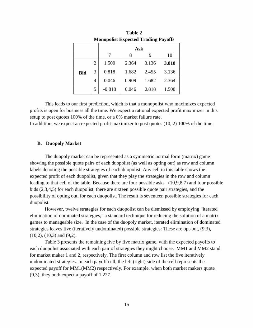
With the previously mentioned reservation prices (vh = 10, vl = 2) in place, the monopolist will choose (am,bm) = (vh,vl) = (10,2) if this results in an expected profit greater than opt-out fee of L$=1.8, which it does (See Table 2). In fact, the expected trading payoff for the monopolist in terms of the (10,2) strategy is L$ = 3.81816

The intuition behind this result is clear. Whenever the monopolist meets a liquidity trader, the quote (10,2) will extract all possible trading surpluses from these traders. At the same time, this very wide bid-ask spread minimizes the monopolist’s losses when she meets an informed trader, since the only true asset values that would be exploited by the informed trader are vt = 1 and vt = 11.

, which is more than double that of the opt-out payoff of L$ = 1.800.

16 Both Monopoly and Duopoly profit values were obtained through an exhaustive spreadsheet computation of all

possible payoffs.

15

Table 2 Monopolist Expected Trading Payoffs

Ask 7 8 9 10

2 1.500 2.364 3.136 3.818

Bid 3 0.818 1.682 2.455 3.136

4 0.046 0.909 1.682 2.364

5 -0.818 0.046 0.818 1.500

This leads to our first prediction, which is that a monopolist who maximizes expected profits is open for business all the time. We expect a rational expected profit maximizer in this setup to post quotes 100% of the time, or a 0% market failure rate. In addition, we expect an expected profit maximizer to post quotes (10, 2) 100% of the time.

B. Duopoly Market

The duopoly market can be represented as a symmetric normal form (matrix) game showing the possible quote pairs of each duopolist (as well as opting out) as row and column labels denoting the possible strategies of each duopolist. Any cell in this table shows the expected profit of each duopolist, given that they play the strategies in the row and column leading to that cell of the table. Because there are four possible asks (10,9,8,7) and four possible bids (2,3,4,5) for each duopolist, there are sixteen possible quote pair strategies, and the possibility of opting out, for each duopolist. The result is seventeen possible strategies for each duopolist.

However, twelve strategies for each duopolist can be dismissed by employing “iterated elimination of dominated strategies,” a standard technique for reducing the solution of a matrix games to manageable size. In the case of the duopoly market, iterated elimination of dominated strategies leaves five (iteratively undominated) possible strategies: These are opt-out, (9,3), (10,2), (10,3) and (9,2).

Table 3 presents the remaining five by five matrix game, with the expected payoffs to each duopolist associated with each pair of strategies they might choose. MM1 and MM2 stand for market maker 1 and 2, respectively. The first column and row list the five iteratively undominated strategies. In each payoff cell, the left (right) side of the cell represents the expected payoff for MM1(MM2) respectively. For example, when both market makers quote (9,3), they both expect a payoff of 1.227.

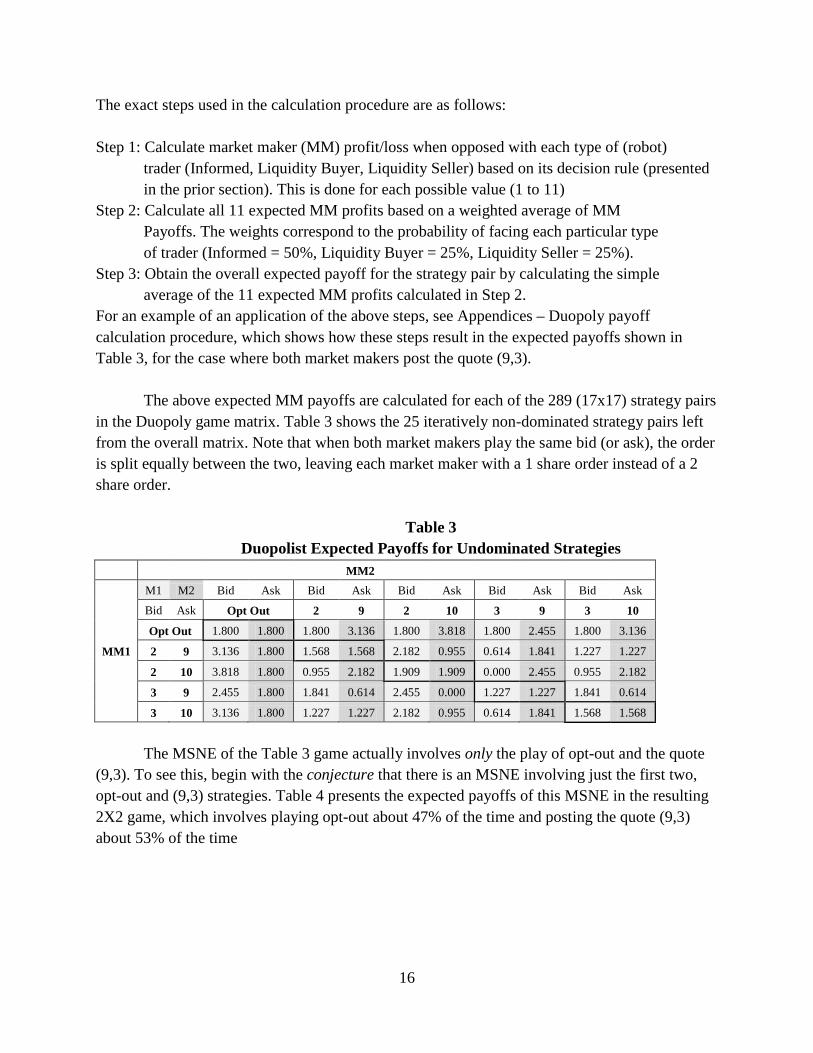
16

The exact steps used in the calculation procedure are as follows: Step 1: Calculate market maker (MM) profit/loss when opposed with each type of (robot)

trader (Informed, Liquidity Buyer, Liquidity Seller) based on its decision rule (presented in the prior section). This is done for each possible value (1 to 11)

Step 2: Calculate all 11 expected MM profits based on a weighted average of MM Payoffs. The weights correspond to the probability of facing each particular type of trader (Informed = 50%, Liquidity Buyer = 25%, Liquidity Seller = 25%).

Step 3: Obtain the overall expected payoff for the strategy pair by calculating the simple average of the 11 expected MM profits calculated in Step 2.

For an example of an application of the above steps, see Appendices – Duopoly payoff calculation procedure, which shows how these steps result in the expected payoffs shown in Table 3, for the case where both market makers post the quote (9,3).

The above expected MM payoffs are calculated for each of the 289 (17x17) strategy pairs in the Duopoly game matrix. Table 3 shows the 25 iteratively non-dominated strategy pairs left from the overall matrix. Note that when both market makers play the same bid (or ask), the order is split equally between the two, leaving each market maker with a 1 share order instead of a 2 share order.

Table 3

Duopolist Expected Payoffs for Undominated Strategies MM2

M1 M2 Bid Ask Bid Ask Bid Ask Bid Ask Bid Ask

Bid Ask Opt Out 2 9 2 10 3 9 3 10

Opt Out 1.800 1.800 1.800 3.136 1.800 3.818 1.800 2.455 1.800 3.136

MM1 2 9 3.136 1.800 1.568 1.568 2.182 0.955 0.614 1.841 1.227 1.227

2 10 3.818 1.800 0.955 2.182 1.909 1.909 0.000 2.455 0.955 2.182

3 9 2.455 1.800 1.841 0.614 2.455 0.000 1.227 1.227 1.841 0.614

3 10 3.136 1.800 1.227 1.227 2.182 0.955 0.614 1.841 1.568 1.568

The MSNE of the Table 3 game actually involves only the play of opt-out and the quote

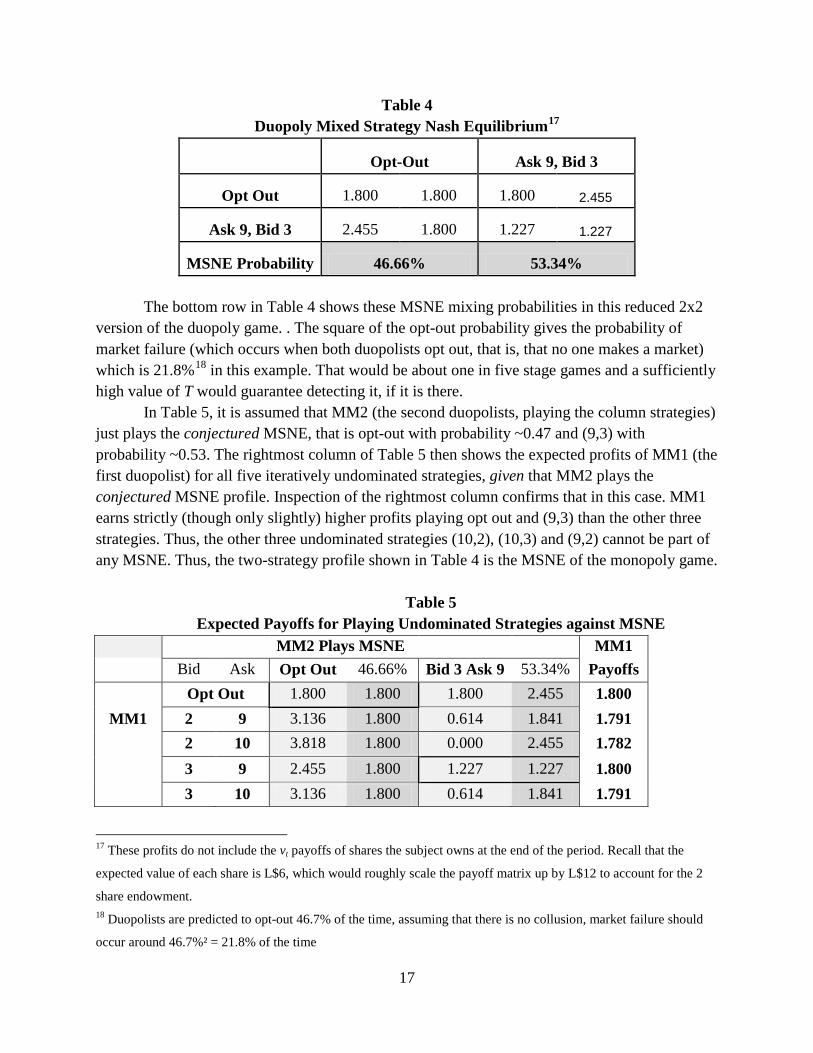
(9,3). To see this, begin with the conjecture that there is an MSNE involving just the first two, opt-out and (9,3) strategies. Table 4 presents the expected payoffs of this MSNE in the resulting 2X2 game, which involves playing opt-out about 47% of the time and posting the quote (9,3) about 53% of the time

17

Table 4 Duopoly Mixed Strategy Nash Equilibrium17

Opt-Out Ask 9, Bid 3

Opt Out 1.800 1.800 1.800 2.455

Ask 9, Bid 3 2.455 1.800 1.227 1.227

MSNE Probability 46.66% 53.34% The bottom row in Table 4 shows these MSNE mixing probabilities in this reduced 2x2

version of the duopoly game. . The square of the opt-out probability gives the probability of market failure (which occurs when both duopolists opt out, that is, that no one makes a market) which is 21.8%18

In Table 5, it is assumed that MM2 (the second duopolists, playing the column strategies) just plays the conjectured MSNE, that is opt-out with probability ~0.47 and (9,3) with probability ~0.53. The rightmost column of Table 5 then shows the expected profits of MM1 (the first duopolist) for all five iteratively undominated strategies, given that MM2 plays the conjectured MSNE profile. Inspection of the rightmost column confirms that in this case. MM1 earns strictly (though only slightly) higher profits playing opt out and (9,3) than the other three strategies. Thus, the other three undominated strategies (10,2), (10,3) and (9,2) cannot be part of any MSNE. Thus, the two-strategy profile shown in Table 4 is the MSNE of the monopoly game.

in this example. That would be about one in five stage games and a sufficiently high value of T would guarantee detecting it, if it is there.

Table 5

Expected Payoffs for Playing Undominated Strategies against MSNE MM2 Plays MSNE MM1 Bid Ask Opt Out 46.66% Bid 3 Ask 9 53.34% Payoffs Opt Out 1.800 1.800 1.800 2.455 1.800

MM1 2 9 3.136 1.800 0.614 1.841 1.791 2 10 3.818 1.800 0.000 2.455 1.782

3 9 2.455 1.800 1.227 1.227 1.800 3 10 3.136 1.800 0.614 1.841 1.791

17 These profits do not include the vt payoffs of shares the subject owns at the end of the period. Recall that the

expected value of each share is L$6, which would roughly scale the payoff matrix up by L$12 to account for the 2

share endowment. 18 Duopolists are predicted to opt-out 46.7% of the time, assuming that there is no collusion, market failure should

occur around 46.7%² = 21.8% of the time

18

It needs to be pointed out that this game was “engineered” to maximize the opt-out probability, and that this implies that the strategies (10,2), (9,3) and (10,3) are “just on the border” of being profitable (they are dominated by playing the MSNE mixture, but just barely). In other words: we constructed the duopoly game to make market failure as likely as possible given the trader setup. This is important because deviations to these unpredicted strategies will involve relatively small payoff consequences, as Table 5 makes clear. That is the reason that a QRE (which we discuss below in Section V) turns out to be a very useful tool to understand the experimental results.

C. Welfare Prediction Our market design has the desirable quality that it unambiguously presents a clear

superior welfare prediction in favor of the monopoly vs. the duopoly under a severe asymmetric information environment. In this design, the monopolist is predicted to always submit quotes while the duopolists sometimes don’t (when they both choose to opt-out, expected to be around 21.8% of the time). This design presents a situation in which Glosten’s prediction of the superiority of the Monopolist specialist vs. Competitive market makers in the face of severe asymmetric information can be clearly tested.

By comparing the two models, a narrower bid-ask spread is predicted in the competitive duopoly market when that market is open, but of course the duopoly market will, on occasion, produce what is in essence an infinite bid-ask spread when the market is closed (when both duopolists opt out).19

Lastly, the prediction that other dominated (Monopoly) and iteratively dominated strategies (Duopoly) will not be chosen can also be examined with this design.

Formally speaking, the MSNE generated in the duopoly model is a zero (trading) profit prediction when one considers that the opt-out fee is really a fixed cost of doing business. Since MSNE profits are determined by that outside option, this duopoly MSNE is an exact game theoretic analogue of the zero profit assumption for competitive market makers imposed in Glosten (1989). The difference of course is that by entering the theoretical world of the MSNE, one is not forced to impose a “zero profit competitive equilibrium” which, as Glosten points out, need not exist with asymmetric information. But an MSNE always exists, and it is interesting to note that we can implement the zero profit equilibrium as an MSNE of a Bertrand pricing game and still get a theoretical prediction like that of Glosten.

V. SUMMARY AND ANALYSIS OF RESULTS

A. Summary

19 Most field data studies examine the bid-ask spread in their comparison of specialist and multiple dealer markets,

but our experimental framework provides an avenue to examine the differences in the bid-ask spread between the

two market mechanisms under identical information asymmetry environments.

19

There are three main findings in this study. First, contrary to the predicted “Glosten result”, duopoly markets were more resilient than monopoly markets under an environment with severe asymmetric information. This is because monopolists chose to opt out in significantly high rates (much higher than the predicted 0%), and duopolists chose to opt out in significantly lower rates than predicted the predicted 47%. We explored possible explanations to these phenomena. The data reveals strong evidence that subjects exhibit “stochastic maximization” behavior that significantly deviates from the MSNE predictions in both markets. In addition, behavioral factors deviating from strict expected profit maximization, such as loss and risk aversion, seem to be significant factors explaining observed monopolist behavior, but less so in the case of duopoly behavior. The rest of this section is structured as follows. First, we summarize the opt out rates for both monopoly and duopoly markets across three time intervals (all periods, last half, and last quarter). Then, we conduct a series of statistical hypothesis tests surrounding the predictions on these opt out rates. This includes the key test of market closure rate comparison between the two markets, which is where we find evidence that rejects the predicted “Glosten result”. Afterwards, we look further into the details of the dealer behavior which suggests that stochastic maximization should be factored into the predictions. This leads to our finding that a Quantal Response Equilibrium (QRE) model (McKelvey and Palfrey 1995) with a single noise parameter generates predictions that allow us to explain some of the experimental results, including a significantly higher than zero prediction of monopolist opt out behavior that is predicted by pure, noiseless expected value maximization, and significantly lower rates of opt out behavior in duopoly than is predicted in the MSNE. Since these two facts strongly characterize our actual results, we believe this is strong evidence that the noisy, stochastic maximization of QRE (rather than pure noiseless maximization of MSNE) is in fact characteristic of our subjects’ behavior. Finally, we explore the use of loss and risk aversion parameters in addition to QRE to find that while this improves the predictions surrounding the monopoly market significantly, it does not improve predictions for the duopoly market.

B. Opt Out Frequency Analysis

In order to facilitate a concrete understanding of the statistical tests employed in this section, let’s first define some terms:

Let 𝑦𝑦𝑡𝑡𝑠𝑠 = 1 if subject s opted out in period t, and zero otherwise. Then we can compute the proportion of times that subject s opts out over some range of periods (𝑗𝑗𝑟𝑟 ,𝑘𝑘𝑟𝑟) in either the monopoly or duopoly runs denoted by r = m or d respectively, as follows: 𝑦𝑦𝑠𝑠(𝑗𝑗𝑟𝑟 ,𝑘𝑘𝑟𝑟) = (𝑘𝑘𝑟𝑟 − 𝑗𝑗𝑟𝑟 + 1)−1 ∑ 𝑦𝑦𝑡𝑡𝑠𝑠

𝑘𝑘𝑟𝑟𝑡𝑡=𝑗𝑗𝑟𝑟 .

The period ranges (𝑗𝑗𝑑𝑑 ,𝑘𝑘𝑑𝑑) and (𝑗𝑗𝑚𝑚 ,𝑘𝑘𝑚𝑚 ) can be all periods of both runs, that is the ranges

(1,80) and (1,40) respectively, or we can use “later” period ranges such as (41,80) and (21,40) to see whether the conclusions are robust after allowing for a period of learning.

20

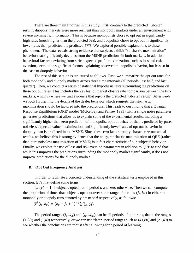
a. Monopoly Market

Recall that we have 36 subjects in all, and that each one of them plays 40 monopoly games, for a total of 1440 monopoly game observations. Contrary to the prediction from expected profits maximization, monopolists opted out in 308 of those 1440 periods, or 21.4% of the time. Nor is there evidence that subjects are learning not to play the opt-out strategy: In fact, Table 6 shows that opt-out was chosen slightly more by the monopolists in later periods than in all periods, though the change is not significant.

Table 6 Proportion of All Monopoly Market Periods in which Subjects Opt Out20

Monopoly Runs (40 periods) All Periods (1–40) Last Half (21-40) Last Quarter (31-40)

Mean 21.4% 23.2% 23.1%

Median 18.7% 20.0% 20.0% Hypothesis test results for the monopoly markets are presented in Table 7. It shows that the point prediction that monopolists opt-out in negligible rates (<5%) is soundly rejected by both the t test and the Wilcoxon (rank-sum) test.

Table 7 Monopoly Market Opt Out Prediction Test

One sample one-tailed tests of null hypothesis that Monopolists

“opt out” hardly at all (0.05 proportion or less of all periods)

Monopoly All Periods (1–40) Last Half (21-40) Last Quarter (31-40)

t-Test p < 0.0001 p < 0.0001 p = 0.0001

Wilcoxon signed rank test

p < 0.0001 p = 0.0001 p = 0.0008

Note that the tests in Table 7 treat each subject’s opt-out proportion as a single observation, and hence are based on 36 observations.

20 Notes: Figures in Tables 6 are based on the proportion of all periods (within the indicated range of periods) that

each subject opts out. Thus, the medians are the “median of subject mean proportions.”

21

The high rate at which monopolists chose to opt out was quite surprising at first since as

pointed out earlier, the expected trading payoff for monopolists employing the dominant strategy of (10, 2) is L$3.82, which is more than double the opt-out fee (L$1.80). We will explore possible explanations in the later sections.

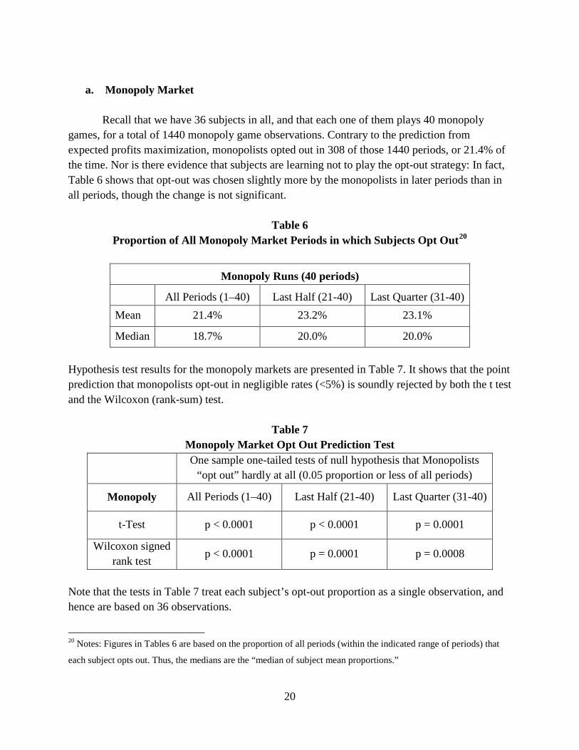
b. Duopoly Market

Recall that in the duopoly treatment, each of our 36 subjects is randomly rematched with another subject in paired games. Since each of the duopolists play 80 duopoly games, a total of 2880 duopolist quote/opt-out observations were generated. (A note of clarification on duopolist observations vs. games: Due to the paired nature of the games, 1440 duopoly games were generated, but since each duopoly game had two dealers, 2880 duopolist observations were generated in total.)

As can be seen in Table 8, the results in the duopoly markets indicate significantly lower opt-out rates than predicted by the MSNE predictions. Duopolists opted out in 891 of those 2880 duopolist observations, or 30.9% of the time. This result appears to be robust to potential learning effects. When looking across the various periods, there does not seem to be any clear evidence of trends towards a higher or lower opt-out rate. In fact, the opt-out strategy was chosen at about the same rate by the duopolists in later periods as in all periods.

Table 8

Proportion of All Duopoly Market Periods in which Subjects Opt Out

Duopoly Runs (80 periods)

All Periods (1–80) Last Half (41-80) Last Quarter (61-80)

Mean 30.9% 30.4% 32.5%

Median 28.7% 26.2% 25.0%

As with the monopolist’s results, the hypothesis test on the duopolist’s side also reject

their predicted opt out rate. While duopolists did choose to opt-out at a higher rate than the monopolists (as predicted by the theories), they did not opt-out (30.9%) at the rate predicted by their MSNE (46.7%). Test results for the duopoly markets presented in Table 9 shows that the point prediction that duopolists opt-out with probability 0.467 is rejected by both the t test and the Wilcoxon (rank-sum) test.

22

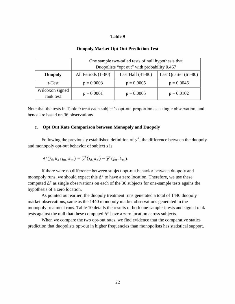
Table 9

Duopoly Market Opt Out Prediction Test

One sample two-tailed tests of null hypothesis that

Duopolists “opt out” with probability 0.467 Duopoly All Periods (1–80) Last Half (41-80) Last Quarter (61-80)

t-Test p = 0.0003 p = 0.0005 p = 0.0046 Wilcoxon signed

rank test p = 0.0001 p = 0.0005 p = 0.0102

Note that the tests in Table 9 treat each subject’s opt-out proportion as a single observation, and hence are based on 36 observations.

c. Opt Out Rate Comparison between Monopoly and Duopoly

Following the previously established definition of 𝑦𝑦𝑠𝑠, the difference between the duopoly and monopoly opt-out behavior of subject s is:

∆𝑠𝑠(𝑗𝑗𝑑𝑑 ,𝑘𝑘𝑑𝑑 ; 𝑗𝑗𝑚𝑚 ,𝑘𝑘𝑚𝑚 ) = 𝑦𝑦𝑠𝑠(𝑗𝑗𝑑𝑑 ,𝑘𝑘𝑑𝑑) − 𝑦𝑦𝑠𝑠(𝑗𝑗𝑚𝑚 ,𝑘𝑘𝑚𝑚 ).

If there were no difference between subject opt-out behavior between duopoly and monopoly runs, we should expect this ∆𝑠𝑠 to have a zero location. Therefore, we use these computed ∆𝑠𝑠 as single observations on each of the 36 subjects for one-sample tests agains the hypothesis of a zero location.

As pointed out earlier, the duopoly treatment runs generated a total of 1440 duopoly market observations, same as the 1440 monopoly market observations generated in the monopoly treatment runs. Table 10 details the results of both one-sample t-tests and signed rank tests against the null that these computed ∆𝑠𝑠 have a zero location across subjects.

When we compare the two opt-out rates, we find evidence that the comparative statics prediction that duopolists opt-out in higher frequencies than monopolists has statistical support.

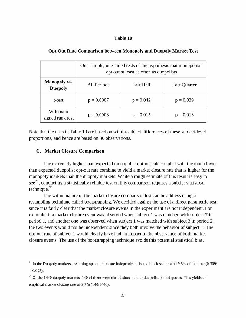
23

Table 10

Opt Out Rate Comparison between Monopoly and Duopoly Market Test

One sample, one-tailed tests of the hypothesis that monopolists opt out at least as often as duopolists

Monopoly vs. Duopoly

All Periods Last Half Last Quarter

t-test p = 0.0007 p = 0.042 p = 0.039

Wilcoxon signed rank test

p = 0.0008 p = 0.015 p = 0.013

Note that the tests in Table 10 are based on within-subject differences of these subject-level proportions, and hence are based on 36 observations.

C. Market Closure Comparison

The extremely higher than expected monopolist opt-out rate coupled with the much lower

than expected duopolist opt-out rate combine to yield a market closure rate that is higher for the monopoly markets than the duopoly markets. While a rough estimate of this result is easy to see21, conducting a statistically reliable test on this comparison requires a subtler statistical technique.22

The within nature of the market closure comparison test can be address using a resampling technique called bootstrapping. We decided against the use of a direct parametric test since it is fairly clear that the market closure events in the experiment are not independent. For example, if a market closure event was observed when subject 1 was matched with subject 7 in period 1, and another one was observed when subject 1 was matched with subject 3 in period 2, the two events would not be independent since they both involve the behavior of subject 1: The opt-out rate of subject 1 would clearly have had an impact in the observance of both market closure events. The use of the bootstrapping technique avoids this potential statistical bias.

21 In the Duopoly markets, assuming opt-out rates are independent, should be closed around 9.5% of the time (0.309²

= 0.095). 22 Of the 1440 duopoly markets, 140 of them were closed since neither duopolist posted quotes. This yields an

empirical market closure rate of 9.7% (140/1440).

24

Specifically, we calculate the observed opt-out rates of each of the 36 subject s over their actual monopoly and duopoly runs. That is, we compute 𝑦𝑦𝑚𝑚

𝑠𝑠 (1,40) and 𝑦𝑦𝑑𝑑𝑠𝑠 (1,80) for each of the

36 subjects. We then populate a computer-simulated experiment with these 36 pairs of subject-specific opt-out rates, where they are binomial probabilities of opting out for each simulated subject. The simulation contains both 40 monopoly periods, and 80 duopoly periods in which simulated subjects are randomly rematched to one another. Each such simulated experiment produces two simulated sample rates of market closure—one in the 40 simulated monopoly periods, and one in the 80 simulated duopoly periods. By repeating this procedure 10,000 times, we bootstrap a confidence interval for the difference between the rate of market closure under duopoly and monopoly. Because this confidence interval is constructed from appropriately correlated market closure events, it takes care of the nonindependence problem described previously.

The bootstrapped confidence interval resulting from this procedure is shown in Table 11. This provides very strong statistical evidence rejecting the hypothesis that monopoly markets are more resilient than duopoly markets (e.g. lower market closure rates)

25

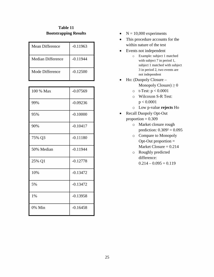
Table 11 Bootstrapping Results

Mean Difference -0.11963

Median Difference -0.11944

Mode Difference -0.12500

100 % Max -0.07569

99% -0.09236

95% -0.10000

90% -0.10417

75% Q3 -0.11180

50% Median -0.11944

25% Q1 -0.12778

10% -0.13472

5% -0.13472

1% -0.13958

0% Min -0.16458

• N = 10,000 experiments • This procedure accounts for the

within nature of the test • Events not independent

o Example: subject 1 matched with subject 7 in period 1, subject 1 matched with subject 3 in period 2, two events are not independent

• Ho: (Duopoly Closure – Monopoly Closure) ≥ 0

o t-Test: p < 0.0001 o Wilcoxon S-R Test:

p < 0.0001 o Low p-value rejects Ho

• Recall Duopoly Opt-Out proportion = 0.309

o Market closure rough prediction: 0.309² = 0.095

o Compare to Monopoly Opt-Out proportion = Market Closure = 0.214

o Roughly predicted difference: 0.214 – 0.095 = 0.119

26

D. A Market Closure Paradox?

The most striking result of this experiment is how much the monopolist dealers

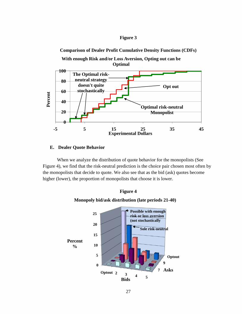
chose to opt-out, when it was very clear that optimal risk-neutral strategy of (10, 2) produced a expected trading profit of L$=3.82, which is more than twice the amount of the opt-out fee (L$=1.8). The clear expected-value maximizing strategy was (10, 2), but in the experiment, it was chosen actually less frequently (16.7%) than the opt-out strategy (23.2%). To explore this perplexing result, we compare the monopolist profits under each strategy in Figure 3 and provide a possible explanation.

To analyze this more fully, recall that the profit figures we have shown so far (in various tables such as Tables 2, 3, 4 and 5) has always been trading profit net of the “endowed earnings” each market maker gets by virtue of being endowed with two units of the asset in each period. When the possible trading profits from the (10, 2) optimal strategy (L$3.82) is combined with the expected vt payoff (L$=12) from the two share endowment in each period, the combined expected profit is L$=15.82. When we do the same for the opt out strategy, we obtain a combined expected profit of L$=13.8.

In relative terms, the difference is much less pronounced. More importantly, as the CDF comparison between the two strategies show, the optimal risk neutral strategy for the monopolist (10, 2) does not quite “stochastically dominate” the opt-out strategy. One CDF stochastically dominates a second CDF if the first CDF lies entirely below the second, and Figure 3 shows that this is not the case. Thus, it is not true that all risk-averse expected utility maximizers would prefer the (10,2) strategy to opting out. This opens the door for the potential of risk and/or loss aversion considerations to provide a possible explanation for these results. This possibility will be explored in the next section. Nevertheless, it is clear that the original prediction based on a risk-neutral expected value maximizing model does not stand up to empirical scrutiny in this experiment.

27

Figure 3

Comparison of Dealer Profit Cumulative Density Functions (CDFs)

E. Dealer Quote Behavior

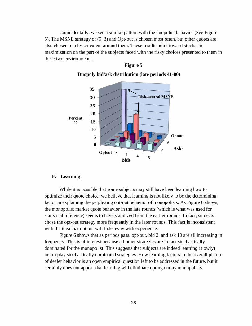
When we analyze the distribution of quote behavior for the monopolists (See Figure 4), we find that the risk-neutral prediction is the choice pair chosen most often by the monopolists that decide to quote. We also see that as the bid (ask) quotes become higher (lower), the proportion of monopolists that choose it is lower.

Figure 4

0

20

40

60

80

100

-5 5 15 25 35 45

Perc

ent

Experimental Dollars

With enough Risk and/or Loss Aversion, Opting out can be Optimal

Optimal risk-neutral Monopolist

Opt out

The Optimal risk-neutral strategy

doesn't quite stochastically

7

9Optout

0

5

10

15

20

25

Optout 2 3 4 5

Asks

Percent%

Bids

Monopoly bid/ask distribution (late periods 21-40)

Sole risk-neutral

Possible with enough risk or loss aversion (not stochastically

28

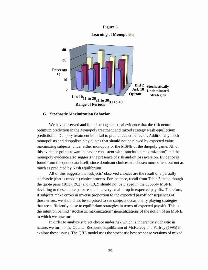
Coincidentally, we see a similar pattern with the duopolist behavior (See Figure 5). The MSNE strategy of (9, 3) and Opt-out is chosen most often, but other quotes are also chosen to a lesser extent around them. These results point toward stochastic maximization on the part of the subjects faced with the risky choices presented to them in these two environments.

Figure 5

F. Learning

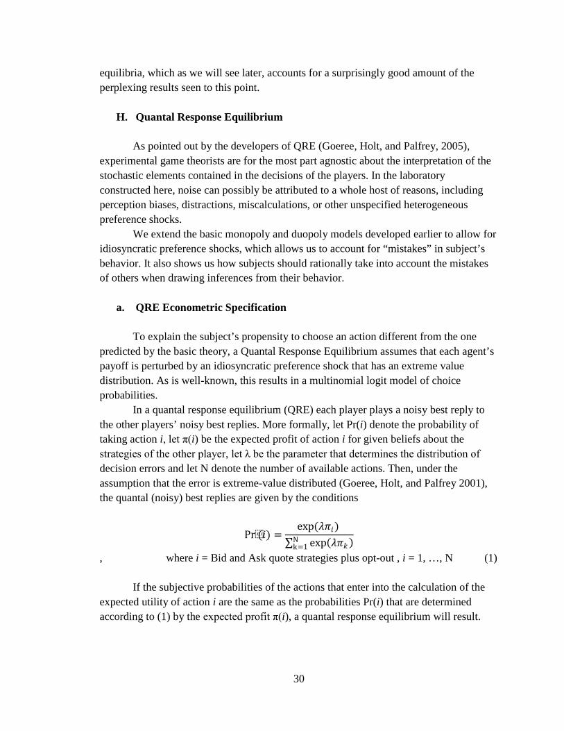
While it is possible that some subjects may still have been learning how to optimize their quote choice, we believe that learning is not likely to be the determining factor in explaining the perplexing opt-out behavior of monopolists. As Figure 6 shows, the monopolist market quote behavior in the late rounds (which is what was used for statistical inference) seems to have stabilized from the earlier rounds. In fact, subjects chose the opt-out strategy more frequently in the later rounds. This fact is inconsistent with the idea that opt out will fade away with experience.

Figure 6 shows that as periods pass, opt-out, bid 2, and ask 10 are all increasing in frequency. This is of interest because all other strategies are in fact stochastically dominated for the monopolist. This suggests that subjects are indeed learning (slowly) not to play stochastically dominated strategies. How learning factors in the overall picture of dealer behavior is an open empirical question left to be addressed in the future, but it certainly does not appear that learning will eliminate opting out by monopolists.

7

9Optout

05

1015202530

35

Optout 2 3 4 5

Asks

Percent%

Bids

Duopoly bid/ask distribution (late periods 41-80)

Risk-neutral MSNE

29

Figure 6

G. Stochastic Maximization Behavior

We have observed and found strong statistical evidence that the risk neutral optimum prediction in the Monopoly treatment and mixed strategy Nash equilibrium prediction in Duopoly treatment both fail to predict dealer behavior. Additionally, both monopolists and duopolists play quotes that should not be played by expected value maximizing subjects, under either monopoly or the MSNE of the duopoly game. All of this evidence points toward behavior consistent with “stochastic maximization” and the monopoly evidence also suggests the presence of risk and/or loss aversion. Evidence is found from the quote data itself, since dominant choices are chosen more often, but not as much as predicted by Nash equilibrium. All of this suggests that subjects’ observed choices are the result of a partially stochastic (that is random) choice process. For instance, recall from Table 5 that although the quote pairs (10,3), (9,2) and (10,2) should not be played in the duopoly MSNE, deviating to these quote pairs results in a very small drop in expected payoffs. Therefore, if subjects make errors in inverse proportion to the expected payoff consequences of those errors, we should not be surprised to see subjects occasionally playing strategies that are sufficiently close to equilibrium strategies in terms of expected payoffs. This is the intuition behind “stochastic maximization” generalizations of the notion of an MSNE, to which we now turn.

In order to analyze subject choice under risk which is inherently stochastic in nature, we turn to the Quantal Response Equilibrium of McKelvey and Palfrey (1995) to explore these issues. The QRE model uses the stochastic best response versions of mixed

OptoutAsk 10

Bid 20

10

20

30

40

1 to 1011 to 2021 to 3031 to 40

Stochastically Undominated

Strategies

Percent%

Range of Periods

Learning of Monopolists

30

equilibria, which as we will see later, accounts for a surprisingly good amount of the perplexing results seen to this point.

H. Quantal Response Equilibrium

As pointed out by the developers of QRE (Goeree, Holt, and Palfrey, 2005), experimental game theorists are for the most part agnostic about the interpretation of the stochastic elements contained in the decisions of the players. In the laboratory constructed here, noise can possibly be attributed to a whole host of reasons, including perception biases, distractions, miscalculations, or other unspecified heterogeneous preference shocks. We extend the basic monopoly and duopoly models developed earlier to allow for idiosyncratic preference shocks, which allows us to account for “mistakes” in subject’s behavior. It also shows us how subjects should rationally take into account the mistakes of others when drawing inferences from their behavior.

a. QRE Econometric Specification To explain the subject’s propensity to choose an action different from the one predicted by the basic theory, a Quantal Response Equilibrium assumes that each agent’s payoff is perturbed by an idiosyncratic preference shock that has an extreme value distribution. As is well-known, this results in a multinomial logit model of choice probabilities. In a quantal response equilibrium (QRE) each player plays a noisy best reply to the other players’ noisy best replies. More formally, let Pr(i) denote the probability of taking action i, let π(i) be the expected profit of action i for given beliefs about the strategies of the other player, let λ be the parameter that determines the distribution of decision errors and let N denote the number of available actions. Then, under the assumption that the error is extreme-value distributed (Goeree, Holt, and Palfrey 2001), the quantal (noisy) best replies are given by the conditions

Pr(𝑖𝑖) =exp(𝜆𝜆𝜋𝜋𝑖𝑖)

∑ exp(𝜆𝜆𝜋𝜋𝑘𝑘)Nk=1

, where i = Bid and Ask quote strategies plus opt-out , i = 1, …, N (1) If the subjective probabilities of the actions that enter into the calculation of the

expected utility of action i are the same as the probabilities Pr(i) that are determined according to (1) by the expected profit π(i), a quantal response equilibrium will result.

31

Note that as the logit precision parameter λ increases, the response functions become more responsive to payoff differences, and the logit response functions converge to the Nash best response functions.

The QRE depends on the precision parameter λ. This must be estimated from the data. This is done in two different ways below: By choosing λ to maximize a log likelihood function, and by choosing λ to minimize the sum of squared errors between predicted and actual strategy choice proportions. Tables 12 and 13 show such estimated models, where the value of λ has been chosen separately for the monopoly and duopoly games.

b. QRE Model Predictions

The predictions of the QRE model (based on the estimated values of λ ) are presented in Table 12 and 1323

We find that the decision rules of the QRE model are qualitatively similar to the empirical choice probabilities in several key respects. In particular, the experimental data qualitatively confirms the prediction of the logistic model that the Duopoly market is more resilient than the Monopoly market structure, and the QRE also predicts most the observed play of strategies not predicted by expected value maximization and the MSNE fairly well.

. As the model show, the predictions are markedly different that those from the basic game-theoretic models developed earlier. The reason for this is twofold: First, because it allows agents to make mistakes and, secondly, because it assumes that agents take into account the possibility that others are also making mistakes when drawing inferences from their actions.

The results from the QRE model, while encouraging, leaves a few issues unresolved. While one can see clearly that the monopolist does have a predicted opt-out probability of 5.6%, it is a far cry from the experimental opt-out rate of 23.2%. What can be the causing the subjects to opt out at such high rates? Stochastic maximization is perhaps part of the answer, but certainly not a complete answer.

I. Prospect Theory and Behavioral Economics

The preference model that gave rise to our initial predictions is the very simple expected value maximization model. One generalization we can pursue is to allow for some risk aversion by using an expected utility model of preferences. But this may not be adequate to our task.

23 The parameter λ was chosen based on two “goodness of fit” measures, the mean square error (MSE) and

the maximum likelihood (ML) statistics.

Table 12 QRE Model Predictions (MSE)

Duopoly Results Market Closure

Monopoly Results Market Closure

5.36%

5.60%

MM1 MM2 Experimental QRE

MM1 MM2 Experimental QRE Bid Ask Proportions Predictionsa Difference

Bid Ask Proportions Predictionsb Difference

Opt out 30.4% 23.14% 7.26%

Opt out 23.2% 5.60% 17.60% 2 7 1.7% 0.71% 0.99%

2 7 2.2% 4.89% -2.69%

2 8 2.4% 4.67% -2.27%

2 8 3.5% 7.21% -3.71% 2 9 4.6% 11.84% -7.24%

2 9 8.2% 10.21% -2.01%

2 10 8.0% 8.83% -0.83%

2 10 16.7% 13.88% 2.82% 3 7 3.7% 0.95% 2.75%

3 7 2.1% 3.60% -1.50%

3 8 5.8% 6.26% -0.46%

3 8 7.5% 5.31% 2.19% 3 9 17.0% 15.87% 1.13%

3 9 11.8% 7.52% 4.28%

3 10 3.8% 11.84% -8.04%

3 10 4.4% 10.21% -5.81% 4 7 3.2% 0.38% 2.82%

4 7 1.9% 2.54% -0.64%

4 8 3.9% 2.47% 1.43%

4 8 4.4% 3.75% 0.65% 4 9 4.7% 6.26% -1.56%

4 9 5.0% 5.31% -0.31%

4 10 3.2% 4.67% -1.47%

4 10 3.9% 7.21% -3.31% 5 7 4.0% 0.06% 3.94%

5 7 0.8% 1.72% -0.92%

5 8 1.0% 0.38% 0.62%

5 8 0.7% 2.54% -1.84% 5 9 1.0% 0.95% 0.05%

5 9 0.4% 3.60% -3.20%

5 10 1.6% 0.71% 0.89%

5 10 3.2% 4.89% -1.69%

a MSE value = 0.001275, λ = 2.30 b MSE value = 0.002537, λ = 0.45

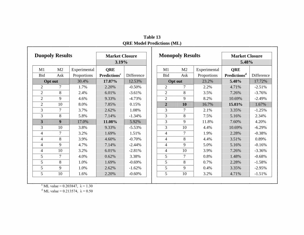
Table 13 QRE Model Predictions (ML)

Duopoly Results Market Closure

Monopoly Results Market Closure

3.19%

5.48%

M1 M2 Experimental QRE

M1 M2 Experimental QRE Bid Ask Proportions Predictionsc Difference

Bid Ask Proportions Predictionsd Difference

Opt out 30.4% 17.87% 12.53%

Opt out 23.2% 5.48% 17.72% 2 7 1.7% 2.20% -0.50%

2 7 2.2% 4.71% -2.51%

2 8 2.4% 6.01% -3.61%

2 8 3.5% 7.26% -3.76% 2 9 4.6% 9.33% -4.73%

2 9 8.2% 10.69% -2.49%

2 10 8.0% 7.85% 0.15%

2 10 16.7% 15.03% 1.67% 3 7 3.7% 2.62% 1.08%

3 7 2.1% 3.35% -1.25%

3 8 5.8% 7.14% -1.34%

3 8 7.5% 5.16% 2.34% 3 9 17.0% 11.08% 5.92%

3 9 11.8% 7.60% 4.20%

3 10 3.8% 9.33% -5.53%

3 10 4.4% 10.69% -6.29% 4 7 3.2% 1.69% 1.51%

4 7 1.9% 2.28% -0.38%

4 8 3.9% 4.60% -0.70%

4 8 4.4% 3.51% 0.89% 4 9 4.7% 7.14% -2.44%

4 9 5.0% 5.16% -0.16%

4 10 3.2% 6.01% -2.81%

4 10 3.9% 7.26% -3.36% 5 7 4.0% 0.62% 3.38%

5 7 0.8% 1.48% -0.68%

5 8 1.0% 1.69% -0.69%

5 8 0.7% 2.28% -1.58% 5 9 1.0% 2.62% -1.62%

5 9 0.4% 3.35% -2.95%

5 10 1.6% 2.20% -0.60%

5 10 3.2% 4.71% -1.51%

c ML value = 0.203847, λ = 1.30

d ML value = 0.213574, λ = 0.50

34

While expected utility has for many decades served as the dominant normative and descriptive model of decision making under uncertainty, it has come under serious question in the modern era. A substantial amount of evidence shows that decision makers violate its basic assumptions on a regular basis across a multitude of economic environments. Many alternative models of choice have been proposed in response to this challenge. Kahneman and Tversky (1979) develop prospect theory to address the failures of expected utility theory, and it was successful in explaining the major violations of expected utility theory in choices between risky prospects.

a. “Behavioral” QRE Model Specification

We incorporate some of the key elements developed in prospect theory to the QRE model developed earlier. In particular, we applied a standard loss aversion and risk aversion framework to the individual dealer payoffs in the entire strategy space. This should not be confused with the cells in the payoff matrix shown earlier in Table 2 and 3. Those payoff values are aggregated from the multiple payoffs values that arise from the combination of every single strategy choice with every possible trader type and asset value. For example, in the duopoly game, the expected value of the [MM1 = (9,3) , MM2 = (9,3)] strategy pair24

was calculated from 33 possible payoffs. The reason was that there are 11 asset values and 3 trader types (11x3 = 33). On one hand, since the monopolist can choose from 17 possible strategies (16 bid/ask combinations and opt-out), a total of 561 (33x17) individual payoff values were adjusted for risk and loss aversion factors. On the other hand, since there is a total of 289 strategy pairs in the duopoly game, a total of 9537 (33x289) individual payoff values were adjusted by adding risk and loss aversion factors to them. This process is essential in order to fully capture exactly the entire spectrum of possible payoffs for both monopoly and duopoly markets.

More formally, with x being the value of every single possible payoff and given a value function V(x), the following parameterization is specified25

V(𝑥𝑥) = �(𝑥𝑥 − 𝑟𝑟)1−𝜌𝜌 𝑓𝑓𝑓𝑓𝑟𝑟 𝑎𝑎𝑎𝑎𝑎𝑎 𝑥𝑥 ≥ 𝑟𝑟,−γ(𝑟𝑟 − 𝑥𝑥)1−ρ for all 𝑥𝑥 ≤ 𝑟𝑟

�

.

where ρ is the coefficient of relative risk aversion, r is the “reference point” γ ≥ 1 is the “loss premium”

After each x was replaced with the new V(x) value function, the QRE was found using the same procedure as in the prior section, yielding what we term the “Behavioral” QRE model. We employed a combination of economic reasoning and a parameter grid search methodology to arrive at the model results seen in Tables 14 and 15. In particular, we found that the reference point of 3.8 was an important

24 See Appendices – Duopoly Payoff Calculation Procedure for exact details. 25 The range for the individual payoffs x that a dealer may face in both monopoly and duopoly markets is from -6 to 40 for

each period. That is, x ∈[-6, 40].

35

parameter to the model. While this reference point differs from the usual 0, which delineates between gains and losses in the traditional sense; we believe there may be valid behavioral reasons why this is not the case in this setting.

Based on how the opt-out strategy is constructed, if the subject chose to opt-out for any particular period, she is guaranteed to receive at least a payoff of L$3.8. The reason is that the lowest payoff of the 2 share endowment was L$2, and the opt-out fee is L$1.8, which adds up to L$3.8 in total. Any subject that chose to opt-out for the period would get a least this amount for sure. It can be argued that this reference point would be the minimum payoff that serves as the basis of judging “gains” vs. “losses”. The loss aversion parameter of 2.25 and the risk aversion parameter of 0.5 are within the range of estimates established in the literature.26

b. “Behavioral” QRE Predictions

Our “behavioral” QRE model indicates that with the inclusion of both risk and loss aversion, a significantly enhanced prediction of Monopolist opt-out rate is achieved. While not to the level of 23.2% as seen in the experiment, the new model does make the prediction that a “behavioral” monopolist would choose to opt-out in the range of 15.7%-17.5% of the time. In addition, the new prediction for the dominant strategy of (10, 2) is almost right on the spot (15%-16.6%) compared to the experiment (16.7%).

The prediction for the opt-out strategy for the Duopolist case is also better, with the new predicted range of opt-out (20%-26.3%) closer to the experimental rate of 30.4%. It should be noted that the (9, 3) and other quote strategy predictions in this new model are in general worse than the predictions obtained in the basic QRE model with expected value preferences. Overall, the “behavioral” QRE is model is significantly better predictor for the Monopoly case than the basic QRE model, but it does no better job at predicting experimental results for the Duopoly case.

Why the “Behavioral” enhancements work for the Monopoly case but not for the Duopoly case is unclear. There is evidence from some studies that the behavioral adjustments used by researchers that work in simple individual choice experiments do not work as well in a well-functioning marketplace.27

26 See Tversky and Kahneman (1992) for a reference on loss and risk aversion parameter estimates.

Perhaps this should not surprise us: the monopoly treatment, due to the lack of a human trader, is really like an individual choice problem. On the other hand, the duopoly treatment is a game against other people, and the market discipline imposed by the invisible hand of competition and market interactions may be a reflection of what Vernon Smith terms “ecological rationality”. There may be some validity in what Smith states in his Nobel Prize Lecture (2002) on Constructivist and Ecological Rationality in Economics: “Truth is discovered in the form of the intelligence embodied in the rules and traditions that have formed, inscrutably, out of the ancient history of human social interactions.” Replacing robot traders and adding human traders in both treatments would be an obvious way of shedding some light on this predictive dichotomy.

27 See John List (2004) for a comparison between neoclassical theory against prospect theory predictions in a sports card market experiment.

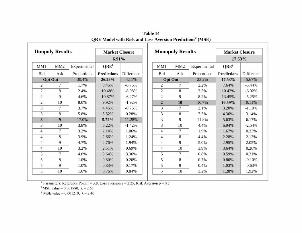
Table 14 QRE Model with Risk and Loss Aversion Predictionse (MSE)

Duopoly Results Market Closure

Monopoly Results Market Closure

6.91%

17.53%

MM1 MM2 Experimental QREf

MM1 MM2 Experimental QREg Bid Ask Proportions Predictions Difference

Bid Ask Proportions Predictions Difference

Opt Out 30.4% 26.29% 4.11%

Opt Out 23.2% 17.53% 5.67% 2 7 1.7% 8.45% -6.75%

2 7 2.2% 7.64% -5.44%

2 8 2.4% 10.48% -8.08%

2 8 3.5% 10.42% -6.92% 2 9 4.6% 10.87% -6.27%

2 9 8.2% 13.45% -5.25%

2 10 8.0% 9.92% -1.92%

2 10 16.7% 16.59% 0.11% 3 7 3.7% 4.45% -0.75%

3 7 2.1% 3.20% -1.10%

3 8 5.8% 5.52% 0.28%

3 8 7.5% 4.36% 3.14% 3 9 17.0% 5.72% 11.28%

3 9 11.8% 5.63% 6.17%

3 10 3.8% 5.22% -1.42%

3 10 4.4% 6.94% -2.54% 4 7 3.2% 2.14% 1.06%

4 7 1.9% 1.67% 0.23%

4 8 3.9% 2.66% 1.24%

4 8 4.4% 2.28% 2.12% 4 9 4.7% 2.76% 1.94%

4 9 5.0% 2.95% 2.05%

4 10 3.2% 2.51% 0.69%

4 10 3.9% 3.64% 0.26% 5 7 4.0% 0.64% 3.36%

5 7 0.8% 0.59% 0.21%

5 8 1.0% 0.80% 0.20%

5 8 0.7% 0.80% -0.10% 5 9 1.0% 0.83% 0.17%

5 9 0.4% 1.03% -0.63%

5 10 1.6% 0.76% 0.84%

5 10 3.2% 1.28% 1.92%

e Parameters: Reference Point r = 3.8, Loss aversion γ = 2.25, Risk Aversion ρ = 0.5 f MSE value = 0.001880, λ = 2.65 g MSE value = 0.001210, λ = 2.40

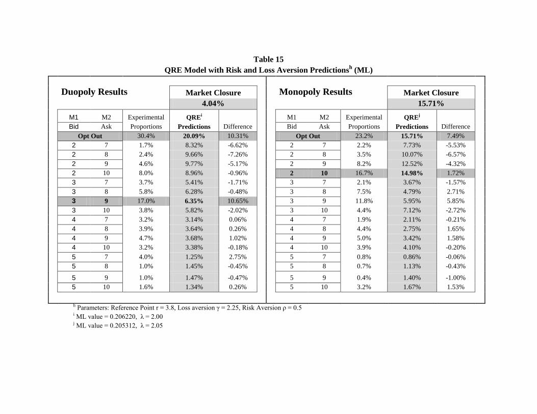
Table 15 QRE Model with Risk and Loss Aversion Predictionsh (ML)

Duopoly Results Market Closure

Monopoly Results Market Closure

4.04%

15.71%

M1 M2 Experimental QREi

M1 M2 Experimental QREj Bid Ask Proportions Predictions Difference

Bid Ask Proportions Predictions Difference

Opt Out 30.4% 20.09% 10.31%

Opt Out 23.2% 15.71% 7.49% 2 7 1.7% 8.32% -6.62%

2 7 2.2% 7.73% -5.53%

2 8 2.4% 9.66% -7.26%

2 8 3.5% 10.07% -6.57% 2 9 4.6% 9.77% -5.17%

2 9 8.2% 12.52% -4.32%

2 10 8.0% 8.96% -0.96%

2 10 16.7% 14.98% 1.72% 3 7 3.7% 5.41% -1.71%

3 7 2.1% 3.67% -1.57%

3 8 5.8% 6.28% -0.48%

3 8 7.5% 4.79% 2.71% 3 9 17.0% 6.35% 10.65%

3 9 11.8% 5.95% 5.85%

3 10 3.8% 5.82% -2.02%

3 10 4.4% 7.12% -2.72% 4 7 3.2% 3.14% 0.06%

4 7 1.9% 2.11% -0.21%

4 8 3.9% 3.64% 0.26%

4 8 4.4% 2.75% 1.65% 4 9 4.7% 3.68% 1.02%

4 9 5.0% 3.42% 1.58%

4 10 3.2% 3.38% -0.18%

4 10 3.9% 4.10% -0.20% 5 7 4.0% 1.25% 2.75%

5 7 0.8% 0.86% -0.06%

5 8 1.0% 1.45% -0.45%

5 8 0.7% 1.13% -0.43%

5 9 1.0% 1.47% -0.47%

5 9 0.4% 1.40% -1.00% 5 10 1.6% 1.34% 0.26%

5 10 3.2% 1.67% 1.53%

h Parameters: Reference Point r = 3.8, Loss aversion γ = 2.25, Risk Aversion ρ = 0.5 i ML value = 0.206220, λ = 2.00 j ML value = 0.205312, λ = 2.05

38

VI. CONCLUSIONS

The main conclusions of this study are the following: Duopoly dealership structure under severe adverse selection is not less viable than

the monopoly dealership structure Duopolists do not quote according to predicted mixed strategy Nash Equilibrium

strategy Dealers do not opt out as much as predicted

Monopolist do not quote according to predicted risk neutral optimum Dealers opt out much more than predicted

A Quantal Response equilibrium model provides a viable explanation for the resiliency of the Duopoly structure in the face of asymmetric information

As we look back at these results obtained in our experiment, a few points of relevance

deserve mention. If we believe that stochastic maximization is common not just in the lab, but in the field as well, then ignoring this can be potentially misleading. In our experiment, we fail to find support for the predicted “Glosten result”. The duopolist’s market structure had tighter spreads and was more resilient to market failure than the monopolist market. The failure of the standard risk-neutral MSNE to properly predict equilibria in games is common in game theory experiments.28

While the design of the experiments carried out in this study were purposely chosen to be as simple as possible in order to create an environment that would not overwhelm the subjects while at the same time provide a rich enough environment to test the “Glosten result”, we see potential avenues of future research that could enhance our understanding of dealer market resiliency.

It also bears mentioning that this is why McKelvey and Palfrey (1995) “invented” QRE.

For example, it would be interesting to investigate thicker markets to allow for market makers to learn from behavior of informed traders and crossing trades. In order to further evaluate the role of competition, it would be interesting to increase the number of market makers and see their impact on spreads and market closure rates. To make the experimental environment closer to what real market makers face, one could incorporate volume and price schedules into the strategy space. A refinement of the trading cost concept may be found in allowing transaction costs to be endogenous to the market. Having human subjects play both the role of dealers and traders could provide richer insights to their behavior.

Back in 1999, when the first two experimental microstructure articles with respect to market transparency were published in RFS, Glosten shared his perspective as a non- 28 See (Goeree and Holt 2001)

39

experimental editor on the use of experiments to shed light on empirical testing of received theories. He acknowledged that the issue of trade-offs associated with transparent vs. nontransparent markets presented difficulties in empirical testing based on field data. The opportunity for a clear test with an exogenous change in institution (transparency) is rare if not nonexistent in real markets. This constraint provided a clear justification for the use of experimental markets, where the institution itself could be controlled exogenously. He also recognized that with simplified institutional structures and many robot participants (e.g. informed and liquidity traders), the behavior of the remaining individuals (e.g. market makers) is isolated and is more easily understood.

We hope to have shown with this study that there are numerous and unforeseen ways in which experimental markets can advance our understanding of how market mechanisms can be affected by key unobserved variables like asymmetric information. Experiments like this one are useful tools that allow for the assessment of policy rules like “to keep markets viable, exchanges may limit the number of seats available to market makers” (Grossman and Miller, 1988). With insights from studies like this one, we will not just be able to improve the design of financial markets, but also gain a better understanding of how human behavior is shaped by its design.

40

APPENDICES

Experimental Instructions

Welcome to the C.T. Bauer College of Business Experimental Research Learning Center! This session has three parts. The first part, which consists of practice dealing periods, is devoted to training you how to use the computer software to make deals and so make money, but there will not be any real money at stake. In the second and third parts, you will “deal for real:” Real money will be at stake. In the session today, you will be a dealer of an imaginary asset. We will call a unit of this asset a share. Your job as a dealer, in each period, is to make offers to buy and sell shares. In the second and third parts of the experiment, you will be a dealer of shares in one of two settings.

• The two settings are either…

o Solo Market: You acting as a sole dealer, OR o Paired Market: You and one other subject, acting as paired dealers.

Your computer screen will tell you which setting you are in at any time, but you will only switch your setting once. That is, in part two you will either be a sole dealer or a paired dealer for all periods, and then in part three you will switch to the other kind of setting.

• Your payment for the study will depend on your performance in this session. Specifically, we calculate winnings as follows:

During this session’s dealing, all money amounts on your computer screen will be denominated in what we will call “lab dollars” or Lab$ for short. Your payment at the end of the session will simply convert all your earnings in Lab$ (from making deals and “share dividends,” described shortly) into U.S. dollars, according to this formula: Payment in US$ = (Total Profits in Lab$) x (1 US$ / 50 Lab$) Your minimum payment is guaranteed to be at least $10. Trading Periods There will be 20 periods of trading in the solo market and 80 periods of trading in the paired market. Shares of the Asset

41

At the beginning of every dealing period, you will automatically receive two shares of the asset. During the period, it is possible that you will sell one or both of those shares. It is also possible that you will buy one or two more shares of the asset. Soon you will learn how you make offers to buy and sell shares, but for the time being, just notice that at the end of any trading period, you may be holding any number of shares between zero shares and four shares of the asset. Share Dividends At the end of each dealing period, each share you hold will disappear or liquidate, and turn into a dividend instead. Any and all shares you may hold will turn into the same dividend. However, the exact dividend is determined by chance: The dividend is “uniformly distributed” on the integers from 1 to 11 Lab$. This means that there is an equal chance that the dividend will be any integer value between 1 and 11. All dividend values from 1 to 11 are equally likely. Notice that the average dividend is 6 Lab$. But remember: Neither you, nor any dealer you may be paired with, will know the dividend value for a dealing period until it ends. The history of dividends you have experienced, as the dealing periods pass, will be clearly shown in a History window on screen. Traders In both market environments you as a dealer will be meeting traders who are interested in buying or selling shares. These traders are actually “computer robots.” They are like computerized opponents in a video game, but much simpler. The other people who are here in today’s session with you are NOT the traders: They are all playing the role of a dealer, just as you are. Shortly, you will learn about different kinds of traders that you might do deals with. But first, let’s learn how you propose deals—this is making offers to buy and sell. How to Trade in an Electronic Limit Order Book Market Trading periods are up to 30 seconds long (except for the practice security). All dealers trade shares by entering orders that (robot) traders can “take”. Which order the trader makes depends on their trader type rule, as described in the trader type section. All orders are for two shares. (The only exception is in the paired market maker environment, where a tie of quotes is results in each dealer buying/selling one share instead of two.)

Trading Gains and Losses

At the beginning of the trading session, you start with a cash endowment of 100 Lab$s. You start each trading period with 2 shares. At the end of the trading period, the shares you own pay the liquidating dividend. The number of shares you own times the liquidating dividend will result in the cash value added to your cash balance for each share you own. At the end of the trading session, your screen will indicate your current trading Lab$ cash total. The final trading Lab$ cash total will serve as the basis for your

42

actual dollar payoff. The exchange rate between the US$s and the Lab$s will be specified at the beginning of the trading exercise. Remember that after your trading period ends, you will start over with 2 shares for the next trading period.

The shares that you used to own from the prior period expire after their corresponding dividend is paid out. Your trading profit in one period has absolutely no effect on the dividends and trader types you face in later periods, they are completely independent from each other. You do not keep any inventory of shares from one period to the next.

Quotes submitted

If you decide to submit an order: o Entering a Bid

A BID is an order to buy shares at a stated price. Click on the bid price at which you are willing to buy shares, and then click SUBMIT. You can choose bid prices from 2 to 5. Remember, the dividend value can be anywhere from 1 to 11 Lab$s. You will buy at that price if a trader chooses to take your bid, and sells shares to you at the price you indicated.

o Entering an Ask

. An ASK is an order to sell shares at a stated price. Click on the ask price at which you are willing to sell shares and then click SUBMIT. You can choose ask prices from 7 to 10. Remember, the dividend value can be anywhere from 1 to 11 Lab$s. You will sell at that price if a trader chooses to take your ask, and buys shares from you at the price you indicated.

Market Bid or Ask: In the paired market maker environment, you will see whether your bid or ask was the best one when the trading period ends and the liquidating dividend is disclosed. Both your quotes and your partner’s quotes will be visible to you after the trading period ends. The history box will also keep a record of both yours’ and your partner’s quotes. In the sole market maker environment, your quotes will be the market quotes automatically. These quotes will also be recorded in the history box.

Default Bid and Ask: The default bid price is No Quote and the default ask price is No

Quote. If you choose to submit a quote, you will have to choose a bid AND a ask price before you can submit quotes. You cannot submit only a bid quote nor only an ask quote.

No Quotes submitted

If you decide NOT to submit an order:

• Click on NO QUOTE

43

Note: You will be paid a 1.8 Lab$s for the period for certain if you choose this course of action. Remember, even if you do not post quotes, you still will receive dividends based on the 2 shares that you already own. By not posting quotes, you will guarantee that you will not buy or sell any shares for that period. Making Offers To Buy and Sell Shares Pay close attention to the decision screen, which you will use to post quotes or opt out. Posting a quote is not a revocable decision once you commit to it, and if you post a quote it is a binding promise to do a deal at the bid and asked prices. Remember that you are allowed to “opt out”, which means you decline to post any quotes and choose to not opt out of playing the role of dealer for that trading period. Sometimes the best choice may to to opt out, which will allow you to totally prevent the chance of facing an informed trader and gain the safe payment of 1.8 Lab$s on top of the dividends of the 2 shares that you will still own. Note: In the paired dealer market, the lowest ask gets all selling action from traders who are interested in buying, and that the highest bid gets all buying action from any traders who are interested in selling, in the event of a tie, the business is split, and each dealer gets to trade one share with the trader. Types of Traders There are three kinds of traders (computer robots) who may come to you to make a deal: 1. Informed Traders

o You may think of Informed Traders as robots with “inside knowledge” that neither you, other dealers nor other kinds of traders have. Specifically, an informed trader knows what the share dividend will be at the end of the trading period, and an informed trader either buys or sells according to what the most profitable trade is for itself, given its superior knowledge. Very specifically, the informed trader does exactly one of these things:

1. BUYS shares from the dealer who has posted the lowest ask price IF this

is less than the dividend value (which, recall, the informed trader already knows);

2. SELLS shares to the dealer who has posted the highest bid price IF this is more than the dividend value (which, recall, the informed trader already knows); or

3. DOES NOTHING if neither of the above situations arise (if the dividend value is between the lowest ask and highest bid prices in that period).

44

Part of your problem, as a dealer, is that “you just can’t win” when you do deals with informed traders. Whenever they sell you shares, the shares will have a lower dividend than the price you pay for them. Whenever they buy shares from you, the shares will have a higher dividend than what they pay you for them. Basically, informed traders take advantage of you dealers! If there were only informed traders to do deals with, it would be in your best interest to always avoid doing deals. And, it may sometimes be in your interest to refuse to do deals. This is why you are allowed to “opt out” as was described previously. But, there are also uninformed buyers and sellers that may do deals with you too. We will talk about them shortly. You can make money dealing with them. So, it may sometimes be in your interest to post bids and asks, instead of opting out.

First, however, let’s look at some examples of deals made with the informed traders.

First, say that the value of the dividend is 9 for that period. Example 1:

If the highest bid price is 4 and the lowest ask price is 8, the INFORMED trader will submit a BUY order for a share of the security at the lowest ask price of 8.

Now, let’s say that the value of the dividend is 7 for that period. Example 2:

If the highest bid price is 4 and the lowest ask price is 8, the INFORMED trader will not submit an order

Lastly, say that the value of the dividend is 3 for that period. Example 3:

If the highest bid price is 4 and the lowest ask price is 8, the INFORMED trader will submit a SELL order for a share of the security at the highest bid price of 4. Now, let’s look at some examples of deals made with uninformed traders, remember you can make money dealing with them. Uninformed Traders

o Uninformed Traders are going to submit a BUY or SELL order irrespective of what the best bid and ask price are for the trading period. 1. Uninformed Buyers will submit a BUY order to buy a share of the security at

the lowest ask price in the market, as long as the ask price is at or below their reservation price of 10. This means that the highest price that uninformed buyers are willing to pay for the shares is 10.

2. Uninformed Sellers will submit a SELL order to sell a share of the security at the highest bid price in the market, as long as the bid price is at or above their reservation price of 2. This means that the lowest price that uninformed sellers are willing to receive for the shares is 2.

45

First, say that the value of the dividend is 9 for that period. Example 1:

If the highest bid price is 4 and the lowest ask price is 8. • A Uninformed BUYER trader will submit a BUY order for a share of the security

at the lowest ask price of 8. • A Uninformed SELLER trader will submit a SELL order for a share of the

security at the highest bid price of 4

Now, let’s say that the value of the dividend is 7 for that period. Example 2:

If the highest bid price is 4 and the lowest ask price is 8. • A Uninformed BUYER trader will submit a BUY order for a share of the security

at the lowest ask price of 8. • A Uninformed SELLER trader will submit a SELL order for a share of the

security at the highest bid price of 4

Lastly, let’s say that the value of the dividend is 3 for that period. Example 3:

If the highest bid price is 4 and the lowest ask price is 8. • A Uninformed BUYER trader will submit a BUY order for a share of the security

at the lowest ask price of 8. • A Uninformed SELLER trader will submit a SELL order for a share of the

security at the highest bid price of 4 Remember, you can may money dealing with uninformed traders. As long as your bid price is 2 or higher, the uninformed seller will be willing to sell shares to you at your bid. As long as your ask price is 10 or lower, the uninformed buyer will also be willing to buy shares from you at your ask. The reservation price of the uninformed buyer is 10, which means they won’t buy shares at a price of 11, and the reservation price of the uninformed seller is 2, which means they won’t sell shares at the price of 1. Keep that in mind as you post quotes.

There is a 50% chance that the trader you encounter is either an Informed trader or a Uninformed trader, if she is a uninformed trader, there is a 50% chance that she will be either a uninformed buyer or seller. This means that there is a 25% chance the she will be a Uninformed Buyer, and a 25% chance that she will be a Uninformed Seller.

Trader Type Selection Probability

One way to see how the random draw of the trader that you will face occurs is to imagine how a coin flip works. Imagine that before each trading period begins, a coin is flipped to decide whether you will be facing an informed trader or a uninformed trader. For illustration, let’s say that heads means that it is an informed trader and tails is a uninformed trader. If it does turns out to be heads, you (and your partner) will face an informed trader. If it turns out tails, then the coin is flipped again and you will either face a uninformed buyer or seller.

46

For illustration, let’s say that heads means it is a buyer and tails means it is a seller. If it does turn out to be heads, then you (and your partner) will face a uninformed buyer and if it turns out tails then you (and your partner) will face a uninformed seller.

During practice sessions, you will know which trader type you encountered after each period in the practice session. This information will be kept in the history box too. This is so that you can familiarize yourself with the software and help you understand how the market works. In the real payoff sessions, you will not know the trader type you encountered during payoff trading sessions. Your history box will also not contain the trader type during the payoff sessions. You will know the dividend paid after each period and in the history box for both types of sessions though. You cash payout will be based on only your trading performance for the payoff sessions. The experimenter will let you know exactly which period is a practice session and which period is a payoff session.

Practice Session vs. Payoff Sessions

Sole Market vs. Paired Market When you make a market in the Sole Market, you will be the only one posting quotes. When you make a market in the Paired Market, you will be posting quotes along with another market maker in the same market. In the case of a tie in the paired market maker market, you and your partner will split the order and each of you will trade one instead of the usual two shares.

Paired Market Specific Instructions

Note: The market bid is the highest bid quoted and the market ask is the lowest ask quoted. The traders will only trade at the market bid and ask.

50%

25%

25%

Trader Type

Informed

Uninformed Seller

Uninformed Buyer

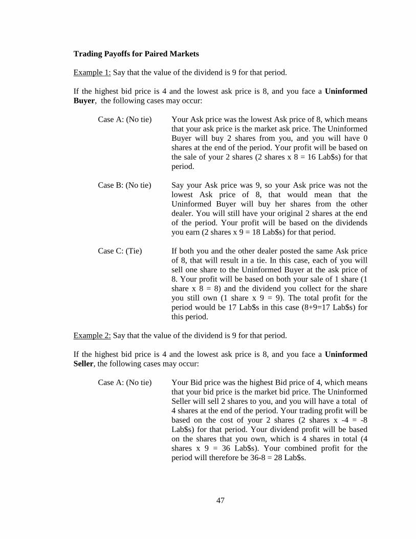
47

Trading Payoffs for Paired Markets Example 1:

Say that the value of the dividend is 9 for that period.

If the highest bid price is 4 and the lowest ask price is 8, and you face a Uninformed Buyer, the following cases may occur:

Case A: (No tie) Your Ask price was the lowest Ask price of 8, which means that your ask price is the market ask price. The Uninformed Buyer will buy 2 shares from you, and you will have 0 shares at the end of the period. Your profit will be based on the sale of your 2 shares (2 shares x 8 = 16 Lab$s) for that period.

Case B: (No tie) Say your Ask price was 9, so your Ask price was not the

lowest Ask price of 8, that would mean that the Uninformed Buyer will buy her shares from the other dealer. You will still have your original 2 shares at the end of the period. Your profit will be based on the dividends you earn (2 shares x 9 = 18 Lab$s) for that period.

Case C: (Tie) If both you and the other dealer posted the same Ask price

of 8, that will result in a tie. In this case, each of you will sell one share to the Uninformed Buyer at the ask price of 8. Your profit will be based on both your sale of 1 share (1 share x 8 = 8) and the dividend you collect for the share you still own (1 share x 9 = 9). The total profit for the period would be 17 Lab$s in this case (8+9=17 Lab$s) for this period.

Example 2:

Say that the value of the dividend is 9 for that period.

If the highest bid price is 4 and the lowest ask price is 8, and you face a Uninformed Seller, the following cases may occur:

Case A: (No tie) Your Bid price was the highest Bid price of 4, which means that your bid price is the market bid price. The Uninformed Seller will sell 2 shares to you, and you will have a total of 4 shares at the end of the period. Your trading profit will be based on the cost of your 2 shares (2 shares x -4 = -8 Lab$s) for that period. Your dividend profit will be based on the shares that you own, which is 4 shares in total (4 shares x 9 = 36 Lab$s). Your combined profit for the period will therefore be 36-8 = 28 Lab$s.

48

Case B: (No tie) Say your Bid price was 3, so your Bid price was not the highest Bid price of 4, that would mean that the Uninformed Seller will sell her shares from the other dealer. You will still have your original 2 shares at the end of the period. Your profit will be based on the dividends you earn (2 shares x 9 = 18 Lab$s) for that period.

Case C: (Tie) If both you and the other dealer posted the same Bid price

of 4, that will result in a tie. In this case, each of you will buy one share from the Uninformed Seller at the bid price of 4. Your trading profit will be based on both your purchase of 1 share (1 share x -4 = -4) and the dividend profit will be based on the dividends you collect for the three shares you now own (3 share x 9 = 27). The total profit for the period would be 23 Lab$s in this case (-4+27=23 Lab$s) for this period.

Example 3:

Say that the value of the dividend is 9 for that period.

If the highest bid price is 4 and the lowest ask price is 8, and you face a Informed Trader, the following cases may occur: Note: The informed trader knows that the actual dividend is 9 for the period, so she will only buy shares at ask prices under 9. Since the Market (lowest) Ask price is 8, the informed trader will buy at that ask price. The informed trader will choose not to sell at the Market Bid price of 4.

Case A: (No tie) Your Ask price was the lowest Ask price of 8, which means that your ask price is the market ask price. The Informed Trader will buy 2 shares from you, and you will have 0 shares at the end of the period. Your profit will be based solely on the sale of your 2 shares (2 shares x 8 = 16 Lab$s) for that period.

Case B: (No tie) Say your Ask price was 9, so your Ask price was not the

lowest Ask price of 8, that would mean that the Informed Trader will buy her shares from the other dealer. You will still have your original 2 shares at the end of the period. Your profit will be based on the dividends you earn (2shares x 9 = 18 Lab$s) for that period.

Case C: (Tie) If both you and the other dealer posted the same Ask price

of 8, that will result in a tie. In this case, each of you will sell one share to the Informed Trader at the ask price of 8.

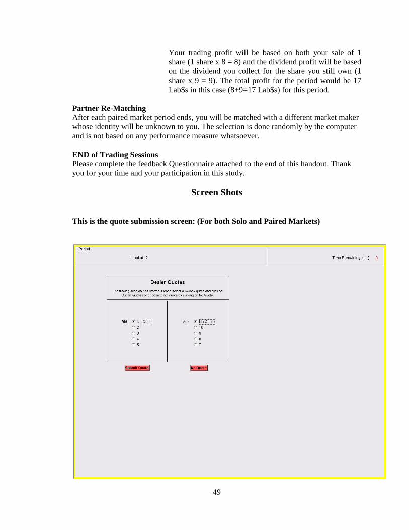
49

Your trading profit will be based on both your sale of 1 share (1 share x 8 = 8) and the dividend profit will be based on the dividend you collect for the share you still own (1 share x 9 = 9). The total profit for the period would be 17 Lab$s in this case (8+9=17 Lab$s) for this period.

Partner Re-Matching After each paired market period ends, you will be matched with a different market maker whose identity will be unknown to you. The selection is done randomly by the computer and is not based on any performance measure whatsoever. END of Trading Sessions Please complete the feedback Questionnaire attached to the end of this handout. Thank you for your time and your participation in this study.

Screen Shots

This is the quote submission screen: (For both Solo and Paired Markets)

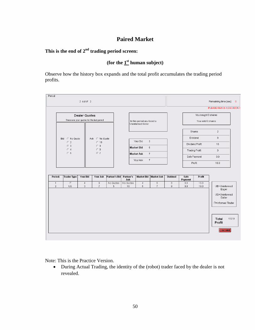
50

Paired Market

This is the end of 2nd trading period screen:

(for the 1st

human subject)

Observe how the history box expands and the total profit accumulates the trading period profits.

Note: This is the Practice Version.

• During Actual Trading, the identity of the (robot) trader faced by the dealer is not revealed.

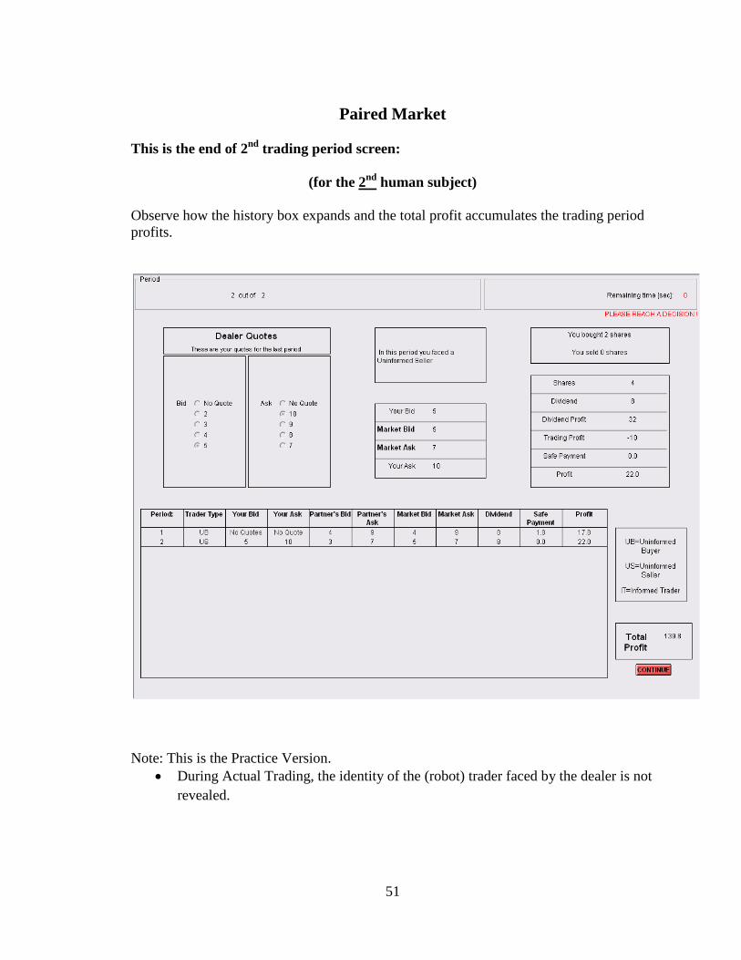
51

Paired Market

This is the end of 2nd trading period screen:

(for the 2nd

human subject)

Observe how the history box expands and the total profit accumulates the trading period profits.

Note: This is the Practice Version.

• During Actual Trading, the identity of the (robot) trader faced by the dealer is not revealed.

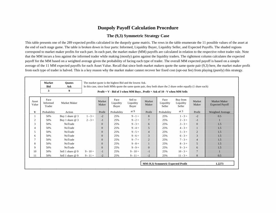
Duopoly Payoff Calculation Procedure The (9,3) Symmetric Strategy Case

This table presents one of the 289 expected profits calculated in the duopoly game matrix. The rows in the table enumerate the 11 possible values of the asset at the end of each stage game. The table is broken down in four parts: Informed, Liquidity Buyer, Liquidity Seller, and Expected Payoffs. The shaded regions correspond to market maker profits for each part. In each part, the market maker (MM) payoffs are calculated in relation to the respective robot trader rule. Note that the MM incurs a loss against the informed trader while making (mostly) gains against the liquidity traders. The rightmost column calculates the expected payoff for the MM based on a weighted average given the probability of facing each type of trader. The overall MM expected payoff is based on a simple average of the 11 MM expected payoffs for each Asset Value. Recall that since both market makers quote the same quote pair (9,3) here, the market maker profit from each type of trader is halved. This is a key reason why the market maker cannot recover her fixed cost (opt-out fee) from playing (purely) this strategy.

Market Quotes The market quote is the highest Bid and the lowest Ask.

Bid Ask In this case, since both MMs quote the same quote pair, they both share the 2 share order equally (1 share each)

3 9

Profit = V - Bid of 3 when MM Buys , Profit = Ask of 10 - V when MM Sells

Asset Value

Face Informed

Trader Market Maker Market

Maker

Face Liquidity

Buyer

Sell to Liquidity

Buyer

Market Maker

Face Liquidity

Seller

Buy from Liquidity

Seller

Market Maker

Market Maker Expected Payoff

V Probability Action Profit Probability at 9 Profit Probability at 3 Profit Weighted Average 1 50% Buy 1 share @ 3 1 - 3 = -2 25% 9 - 1 = 8 25% 1 - 3 = -2 0.5 2 50% Buy 1 share @ 3 2 - 3 = -1 25% 9 - 2 = 7 25% 2 - 3 = -1 1 3 50% NoTrade

0 25% 9 - 3 = 6 25% 3 - 3 = 0 1.5

4 50% NoTrade

0 25% 9 - 4 = 5 25% 4 - 3 = 1 1.5 5 50% NoTrade

0 25% 9 - 5 = 4 25% 5 - 3 = 2 1.5

6 50% NoTrade

0 25% 9 - 6 = 3 25% 6 - 3 = 3 1.5 7 50% NoTrade

0 25% 9 - 7 = 2 25% 7 - 3 = 4 1.5

8 50% NoTrade

0 25% 9 - 8 = 1 25% 8 - 3 = 5 1.5 9 50% NoTrade

0 25% 9 - 9 = 0 25% 9 - 3 = 6 1.5

10 50% Sell 1 share @ 9 9 - 10 = -1 25% 9 - 10 = -1 25% 10 - 3 = 7 1 11 50% Sell 1 share @ 9 9 - 11 = -2 25% 9 - 11 = -2 25% 11 - 3 = 8 0.5

MM (9,3) Symmetric Expected Profit 1.2273

53

BIBLIOGRAPHY

Amihud, Y., T. Ho, and R. Schwartz, 2003, Market Making and the Changing Structure

of the Securities Industry, Beard Books. Bhattacharya, U., and M. Spiegel, 1991, Insiders, Outsiders, and Market Breakdowns,

The Review of Financial Studies, 4, 255-282. Benveniste, L., A. Marcus, and W. Wilhelm, 1992, What’s special about the specialist?,

Journal of Financial Economics, 32, 61-86. Bias, B., 1993, Price Formation and Equilibrium Liquidity in Fragmented and

Centralized Markets, The Journal of Finance, 48 (1), 157-185. Bias, B., D. Martimort, and J. Rochet, 2000, Competing Mechanisms in a Common

Value Environment, Econometrica, 68, 799-837. Bloomfield, R., 1996, Quotes, Prices, and Estimates in a Laboratory Market, The Journal

of Finance, 51, 1791-1808. Bloomfield, R., M. O’Hara, G. Saar, 2009, The Limits of Noise Trading: An

Experimental Analysis, The Review of Financial Studies, 22, 2275-2302. Bondarenko, O., 2001, Competing market makers, liquidity provision, and bid-ask

spreads, Journal of Financial Markets, 4, 269-308. Camerer, C., G. Loewenstein, and M. Rabin, eds., Advances in Behavioral Economics,

2004, Russell Sage Foundation and Princeton University Press. Campbell, J., S. LaMaster, V. Smith, and M. Van Boening, 1991, Off-Floor Trading,

Disintegration, and the Bid-Ask Spread in Experimental Markets, The Journal of Business, 64, 495-522.

Chung, K., and Y. Kim, 2008, Volatility, Market Structure, and the Bid-Ask Spread,

working paper, SUNY Buffalo. Clarke, J., and K. Shastri, 2000, On Information Asymmetry Metrics, working paper,

University of Pittsburg. Dennert, J., 1993, Price Competition between Market Makers, Review of Economic

Studies, 60, 735-751. Easley, D., N. Kiefer, and M. O’Hara, 1997, The information content of the trading

process, Journal of Empirical Finance, 4, 159-186.

54

Ellis, K., R. Michaely, and M. O’Hara, 2002, The Making of a Dealer Market: From Entry to Equilibrium in the Trading of Nasdaq Stocks, The Journal of Finance, 57, 2289-2316.

Feltovich, N., and J. Swierzbinski, 2009, The role of strategic uncertainty in games: an

experimental study of cheap talk and contracts in the Nash demand game, working paper, University of Aberdeen Business School.

Fischbacher, U., 2007, z-Tree: Zurich Toolbox for Ready-made Economic Experiments,

Experimental Economics, 10, 171-178. Flood, M., R. Huisman, K. Koedijk, and R. Mahieu, 1999, Quote Disclosure and Price

Discovery in Multiple-Dealer Financial Markets, The Review of Financial Studies, 12, 37-59.

Fudenberg, D., and J. Tirole, 1991, Game Theory, The MIT Press. George, T., G. Kaul, and M. Nimalendran, 1994, Trading Volume and Transaction Costs

in Specialist Markets, The Journal of Finance, 49, 1489-1506. Germain, L., and F. Rousseau, 2005, Strategic Market Making and Risk Sharing, working

paper, Toulouse Business School. Glosten, L., and P. Milgrom, 1985, Bid, Ask, and Transaction Prices in a Specialist

Market with Heterogenously Informed Traders, Journal of Financial Economics, 21, 123-144.

Glosten, L., 1989, Insider Trading, Liquidity, and the Role of the Monopolist Specialist,

The Journal of Business, 62, 211-235. Glosten, L., 1994, Is the Electronic Limit Order Book Inevitable? The Journal of

Finance, 49, 1127-1161. Goeree, J., C. Holt, 2001, Ten Little Treasures of Game Theory and Ten Intuitive

Contradictions, American Economic Review, 9, 1402-1422. Goeree, J., C. Holt, and T. Palfrey, 2005, Regular Quantal Response Equilibrium,

Experimental Economics, 8, 347-367. Grossman, S., and M. Miller, 1988, Liquidity and Market Structure, The Journal of

Finance, 43, 617-633. Heidle, H., and R. Huang, 2002, Information-based trading in dealer and auction markets:

An analysis of exchange listings, Journal of Financial and Quantitative Analysis, 37, 391-424.

55

Ho. T., and H. Stoll, 1983, The Dynamics of Dealer Markets under Competition, The Journal of Finance, 38, 1053-1074.

Kahneman, D., and A. Tversky, 1979, Prospect Theory: An Analysis of Decision under

Risk, Econometrica, 47, 262-291. Kahneman, D., and A. Tversky, 1992, Advances in Prospect Theory: Cumulative

Representation of Uncertainty, Journal of Risk and Uncertainty, 5, 297-323. Klock, M., and T. McCormick, 1999, The Impact of Market Maker Competition on

Nasdaq Spreads, The Financial Review, 34, 55-73. Köszegi, B., and M. Rabin, 2006, A Model of Reference-Dependent Preferences, The

Quarterly Journal of Economics, 121, 1133-1165. Krahnen, J., and M. Weber, 2001, Marketmaking in the Laboratory: Does Competition

Matter?, Experimental Economics, 4, 55-85. Kyle, A., 1985, Continuous auctions and insider trading, Econometrica, 53, 1315-1335. Lamoureux, C., and C. Schnitzlein, 2004, Microstructure with Multiple Assets: An

Experimental Investigation into Direct and Indirect Dealer Competition, Journal of Financial Markets, 7, 117-143.

List, J., 2004, Neoclassical Theory versus Prospect Theory: Evidence from the

Marketplace, Econometrica, 72, 615-625. McKelvey, R., and T. Palfrey, 1995, Quantal Response Equilibria for Normal Form

Games, Games and Economic Behavior, 10, 6-38. Miller, R., 2002, Experimental Economics: How we can build better financial markets,

John Wiley and Sons, Inc. Neal, R., 1992, A Comparison of Transaction Costs between Competitive Market Maker

and Specialist Market Structures, The Journal of Business, 65, 317-334. Pagano, M., and A. Roell, 1996, Transparency and Liquidity: A Comparison of Auction

and Dealer Markets with Informed Trading, The Journal of Finance, 51, 579-611. Parlour, C., and D. Seppi, 2003, Liquidity-Based Competition for Order Flow, The

Review of Financial Studies, 16, 301-343. Ramos, S., 2003, Competition between Stock Exchanges: A Survey, Research Paper no.

77, HEC-University of Lausanne, FAME and CEMAF/ISCTE.

56

Roth, A.E., 1977a, The Shapley value as a von Neumann-Morgenstern utility,

Econometrica, 45, 657-664. Roth, A.E., 1977b, Bargaining ability, the utility of playing a game, and models of

coalition formation, Journal of Mathematical Psychology, 16, 153-160. Schnitzlein, C., 1996, Call and Continuous Trading Mechanisms Under Asymmetric

Information: An Experimental Investigation, The Journal of Finance, 51, 613-636.

Seppi, D., 1997, Liquidity Provision with Limit Orders and a Strategic Specialist, The

Review of Financial Studies, 10, 103-150. Smith, V. 2002, Constructivist and Ecological Rationality in Economics, Prize Lecture,

George Mason University. Stoll, H., 1992, Principles of Trading Market Structure, Journal of Financial Services

Research, 6, 75-107. Theissen, E., 2000, Market Structure, Informational Efficiency and Liquidity: An

Experimental Comparison of Auction and Dealer Markets, Journal of Financial Markets, 3, 333-363.

Van Boening, M., and N. Wilcox, 1996, Avoidable cost: Ride a double auction roller coaster. American Economic Review, 86, 461-477.

Van Huyck, J., R. Battalio, and R. Beil, 1990, Tacit Coordination Games, Strategic

Uncertainty, and Coordination Failure, The American Economic Review, 80, 234-248.

Venkataraman, K., and A. Waisburd, 2007, The Value of the Designated Market Maker,

Journal of Financial and Quantitative Analysis, 42, 735-758. Wilcox, N., 2008, Stochastic models for binary discrete choice under risk: A critical

primer and econometric comparison. In J. C. Cox and G. W. Harrison, eds., Research in Experimental Economics Vol. 12: Risk Aversion in Experiments pp. 197-292. Bingley, UK: Emerald.