on public inefficiencies in a mixed duopoly
TRANSCRIPT
STRATHCLYDE
DISCUSSION PAPERS IN ECONOMICS
ON PUBLIC INEFFICIENCIES IN A MIXED DUOPOLY
BY
CARLO CAPUANO AND GIUSEPPE DE FEO
NO. 09-16
DEPARTMENT OF ECONOMICS UNIVERSITY OF STRATHCLYDE
GLASGOW
On Public Inefficiencies in a Mixed Duopoly
Carlo CAPUANO1 and Giuseppe DE FEO2
July 2009
Abstract
The aim of this paper is to investigate the welfare effect of a change in the publicfirms objective function in oligopoly when the government takes into account the distor-tionary effect of rising funds by taxation (shadow cost of public funds). We analyze theimpact of a shift from welfare- to profit-maximizing behaviour of the public firm on thetiming of competition by endogenizing the determination of simultaneous (Nash-Cournot)versus sequential (Stackelberg) games using the game with observable delay proposed byHamilton and Slutsky (1990). Differently from previous work that assumed the timing ofcompetition, we show that, absent efficiency gains, instructing the public firm to play as aprivate one never increases welfare. Moreover, even when large efficiency gains result fromthe shift in public firm’s objective, an inefficient public firm that maximizes welfare maybe preferred.
Keywords: Mixed oligopoly; Nash equilibria; Endogenous Timing; Distortionary taxes.
JEL Classification: L1; L13; L32; L33.
1Department of Economics, University of Naples Federico II, Complesso Universitario di Monte S.Angelo,Via Cintia, Napoli, 80126; E-mail: [email protected]
2Department of Economics, University of Strathclyde, Sir William Duncan Building, 130 Rottenrow, Glas-gow G4 0GE, UK. E-mail: [email protected] wish to thank Jean Hindriks, Rabah Amir, Paul Belleflamme, Vincent Vannetelbosch, Pierre Pestieau,Francesca Stroffolini, Antonio Acconcia, Alfredo Del Monte, Oscar Amerighi, Massimo Salzano, AlessandroPetretto, Giacomo Calzolari, Vincenzo Deniccolo and Toshihiro Matsumura. This work also benefitted fromcomments from seminar audiences at Universities of Bologna, Verona, Pavia, Tokyo and Lisbon. The secondauthor is grateful to the Center for Operations Research and Econometrics (CORE) since this work has beenmostly written there when he was PhD student at the Universite catholique de Louvain. The usual disclaimersapply.
1 Introduction
In the last decades of the XX century a process of liberalization and/or privatization occurredin most of the industrialized countries and, since then, public utilities are generally no longerprovided by public monopolies. The motivations for this program were essentially linked tothe general perception of poor performance of public monopolies and to the idea that entry ofprivate subjects could enhance efficiency. For example, during the nineties, in Italy, in Franceand in UK, as in many EU countries, the public incumbent faced the entry of private com-petitors in many communication services. The same occurred in the production of electricity,in gas retailing and more recently in some postal services. In the same years, national (public)airlines started competing with private or foreign ones in the domestic markets. Moreover,examples of public monopolies that became mixed oligopoly can be found in a broad rangeof industries including railways, steel and overnight-delivery industries, as well as servicesincluding banking, home loans, health care, life insurance, hospitals, broadcasting, and edu-cation.1 In these cases, instead of regulating a privatized monopoly, governments decided toenforce a facility-based competitions in order to achieve a so-called dynamic efficiency.2 Inother cases, even if public firms had not been privatized, it was required its management tooperate satisfying the budget balance constraint or to directly maximize profits, as privatefirms do.
Our investigation starts downward the liberalization process of a public monopoly, andthe aim of the present work is to build a theoretical model for analyzing the welfare effectof a change in its objective function in oligopoly3. Since we mainly refer to public utilitymarkets open to competition, we consider a mixed duopoly in which firms are characterizedby increasing returns to scale (with fixed and constant marginal costs) and we assume thatthe public firm is typically less efficient than its private competitor.4
The first novel contribution of this paper is represented by the introduction of the shadowcost of public funds in the public firm’s objective function. That is, we assume that thepublic firm is required to take into account the distortionary effect of the taxes that areneeded to cover its deficit and, in general, public expenditures. In fact, absent lump-sum taxinstruments, if government rises 1 Euro from taxation, society pays (1 + λ) Euros. Coherently,public profits, when positive, avoid an equivalent public transfer, reducing distortionary taxes.5
As initially analyzed in Meade (1944) and exploited in Laffont and Tirole (1986, 1993), thisapproach has been used to characterize public monopolies running a deficit and, more generally,regulated markets. Here we apply the same analysis to a public firm competing in a duopolyand to the effects of privatization or of a change f public firm’ objective function like profit
1In industrial organization the term mixed oligopolies has been used to describe imperfectly competitivemarkets in which public firms compete with private ones.
2For deeper viewpoints on the role played by facility-based competition in EU and US Telecommunicationsliberalization and regulation processes see Taschdjian (1997) and Stehmann and Borthwick (1994).
3This change can be the consequence not only of a privatization process but also of a political choice.4Differently from Cremer et al. (1989), the public firm’s higher cost is not a neutral transfer from firm to
workers belonging to the same economy but, as an X−inefficiency, it reduces any utilitarian measure of welfare.Moreover, we can represent with an extra cost any problem of controlling and/or monitoring that derive fromagency problem that affect public firms but that we don’t analyze. Notice that we do not consider that in anycontext public firms are less efficient than private competitors, but we start from the worst context and weprove that inefficiency cannot matter.
5Since public firm’s profit or deficit are not a neutral transfer among agents of the same economy, they oughtnot to be weighted as private firm’s profits or consumer net surplus in the utilitarian measure of welfare, butthey should be weighted (1 + λ).
1
maximization, given that getting money for reducing public debt or distortionary taxes, is oftena complementary target6. The main consequence is that, taking into account the shadow costof public funds, the public firm puts more weight on its own profits mimicking, at leastpartially, the behaviour of a private firm.
The second contribution of this work is that we consider the effect of a change in the publicfirm’s objective function on the timing of competition by endogenizing the determination ofsimultaneous (Nash-Cournot) versus sequential (Stackelberg) games. That is, the structure ofthe game is not assumed a priori, but is the result of preplay independent and simultaneousdecisions by the players. In fact, in many economic situations it is often more reasonable toassume that firms choose not only what action to take, but also when to take it. Moreover,we believe that this approach is especially relevant for the analysis of privatization, given thatresults and policy prescriptions emerged in the literature crucially rely on the type of competi-tion assumed. For example, in de Fraja and Delbono (1989) it is shown that privatization mayimprove welfare under Cournot competition even without efficiency gains; while, if a Stack-elberg game with public leadership is exogenously assumed, this cannot occur.7 In anotherpaper, Beato and Mas-Colell (1984) show that welfare may be higher when the public firm isthe follower than when it is the leader in a Stackelberg game. In this way they provided anargument against the standard view of the so-called Second-Best literature (see, for example,Rees, 1984; Bos, 1986) that claimed the sub-optimality of the marginal-cost pricing rule.8
In the present work, in order to endogenize the timing of the game, we apply the model de-veloped by Hamilton and Slutsky (1990) to the mixed oligopoly framework. In their insightfulpaper, the authors build an endogenous timing game by adding to the basic quantity gamea preplay stage at which players simultaneously and independently decide whether to moveearly or late in the basic game. Therefore, the type of competition endogenously emerges inthe subgame-perfect equilibrium (SPE) of this extended game. Amir and Grilo (1999) applythis model to a private duopoly showing that, in a quantity setting with strategic substi-tutability, Cournot equilibria always result as the SPE of the endogenous timing game. Pal(1998) addresses the issue of endogenous order of moves in a mixed oligopoly by adopting thesame game structure. It is shown that sequential playing always emerges as the endogenoustiming and both Stackelberg solutions are the SPE of the mixed-duopoly game. Even thoughafter Pal (1998) other authors analyzed the endogenous timing in mixed oligopolies, there isno work, at our best knowledge, that extends this line of research to the welfare evaluation ofprivatization.9
The main results of our analysis can be summed up as follows.With respect to the determination of the endogenous timing in mixed oligopoly, our results
differ from Pal (1998), since in our model setting either Nash, or private leadership or bothStackelberg outcomes can result as subgame-perfect equilibria (SPE) of the endogenous timinggame. Moreover, following the intuition of Beato and Mas-Colell (1984), we show that whenboth Stackelberg game are SPE of the endogenous timing game, private leadership is preferred
6Given our model setting, it will be clear than there is no differences between to privatize a public firm andto ask its management to maximize no welfare but profits. This case is what we call a change in the publicfirm’s objective function.
7The assumption of decreasing returns to scale is fundamental to their result that privatization may increaseswelfare. This is generally not the case of a public utility provider.
8See de Fraja and Delbono (1990) for a survey of these models.9Matsumura (2003), Cornes and Sepahvand (2003) and Sepahvand (2004) apply the same model to interna-
tional mixed oligopolies finding that public leadership may emerge as the unique SPE of the endogenous timinggame.
2
by the public firm and it is indeed selected when risk-dominance is used as the equilibriumselection criterion.
This result is crucial to the evaluation of the welfare impact of asking a public firm tomaximize profits. In fact, differently from de Fraja and Delbono (1989), absent efficiencygains, profit maximization never increases welfare. Furthermore, even when large efficiencygains are realized, an inefficient public firm that maximize welfare may still be preferred. Thelast result relies on the fact that only with a public firm sequential outcomes (that are alwayswelfare superior) may be supported as SPE of the endogenous timing game. Conversely, withprivate-owned firms, simultaneous equilibria are always implemented.
It is worth noting that our results are obtained in a context of complete information,and under the assumption that government has the full bargaining power in the privatizationprocess; that is, the price paid by the new private owners for the former public firm is assumedto be equal to its profit in the new (Cournot) equilibrium. This assumption drives the resultsin favour of privatization or of asking public firms to maximize profits, since it overweightsthe profits by λ in any welfare comparison.
In what follows, the next Section sets up the model. Section 3 is focused on the issue ofendogenous timing in mixed oligopoly, while Section 4 is devoted to the analysis of a changeof the public firm’s objective function. Our conclusions are delegated to Section 5. All theproofs are collected in the Appendix.
2 The basic setting
In a static, partial equilibrium analysis, we consider the simplest setting of a mixed duopoly,where a private and a public firm, labelled with i = p, g respectively, produce a commodityand compete in a quantity game. Demand preferences are described by a linear function whereintercept and slope are normalized to one:
p (qg, qp) = 1− qp − qg
Both firms are characterized by constant marginal costs, ci ≥ 0, and fixed costs, Ki ≥ 0 10.We assume that the public firm is already in the market and its fixed cost is sunk. Conversely,the private firm’s fixed cost is borne only in case of producing. Moreover, the private firm’smarginal cost is normalized to zero, cp = 0, while the public firm’s one is positive, cg = c ≥ 0.That means, c is an index of the public firm’s inefficiency.
The private firm maximizes its profit:
Πp (qg, qp) = (1− qg − qp) qp −Kp
The public firm maximize a utilitarian measure of welfare taking into account the shadow costof public funds, λ > 0. This parameter is a measure of the dead-weight loss due to distortionarytaxation. In particular, let S(Q) denote the consumer gross surplus, where Q = qp + qg is theindustry total output. We assume that government can choose the public firm’s output level
10We consider that the assumption of increasing returns to scale is coherent with the presence of a publicincumbent, former monopolist, in a liberalized public utility industry. Nevertheless, the assumption decreasingreturn to scale is popular in the literature. For papers adopting constant marginal costs, see Cremer et al.(1989) and Martin (2004); while for papers adopting increasing marginal costs, see Beato and Mas-Colell (1984),de Fraja and Delbono (1989), Fjell and Pal (1996), Pal and White (1998), Matsumura (1998).
3
qg and it can make a monetary transfer T to the public firm. Then, in the presence of theshadow cost of public funds, the maximization problem of the government is:
maxqg ,T
W (qp, qg) = S(qp + qg)− Cg(qg)− Cp(qp)− λT
such that Πg = p(qp + qg)qg − Cg(qg)−Kg + T ≥ 0 (1)
where Πg is the public firm’s budget including the (positive or negative) transfer T . Notice thatthe (participation) constraint (1) is not a hard budget balance constraint but it is compatiblewith operative losses when T is positive. From (1) we get
T = Πg − [p(Q)qg − Cg(qg)−Kg]
and substituting T in the objective function we obtain:
maxqg
W = S(qp + qg)− Cg(qg)− Cp(qp)− λ[Πg − (p(Q)qg − Cg(qg)−Kg)
]= S(qp + qg)− Cg(qg)− Cp(qp) + λ (p(Q)qg − Cg(qg)−Kg)− λΠg
such that Πg ≥ 0
Since welfare is decreasing in Πg when λ is positive, it is optimal to set Πg = 0. Then, wehave:
T = − [p(Q)qg − Cg(qg)−Kg]
The problem can be rewritten unconstrained as follows:
maxqg
W = S(qp + qg)− Cg(qg)− Cp(qp) + λ (p(Q)qg − Cg(qg)−Kg)
Defining the consumer net surplus as
CS(Q) = S(Q)− p(Q)(qp + qg) (2)
and the public firm’s operative profit as
Πg (qg, qp) = p(Q)qg − Cg(qg)−Kg (3)
the maximization problem of the government is reduced to:
maxqg
W (qg, qp) = CS(Q) + Πp (qg, qp) + (1 + λ)Πg (qg, qp) (4)
So, the objective defined in equation (4) implies that a transfer occurs in order to guaranteethe public firm’s budget balance. This transfer is positive (negative) when the public firm’sprofits are negative (positive).
The objective function (4) can be also interpreted as a weighted average of welfare, definedas the net surplus generated in the market, and the public firm’s profit, where the former isweighted by 1/(1 + λ), the latter by λ/(1 + λ).
W (qg, qp) = V (qg, qp) + λΠg (qg, qp) (5)
m1
1 + λV (qg, qp) +
λ
1 + λΠg (qg, qp)
4
where V (qg, qp) = CS(Q) + Πg (qg, qp) + Πp (qg, qp)
We know that other works on mixed oligopoly consider a weighted average of welfare aspublic firm’s objective function. In fact, if we had assumed a hard budget balance constraintwithout a public transfer, as in Cremer et al. (1989), the weight given to the public firm’s profitwould have been endogenous and equal to the associate Lagrangian multiplier. Alternatively,as in Hindriks and Claude (2006) the weight could be positively related to the endogenous shareof a partially privatized firm owned by private investors, while as in Matsumura (1998), dueto incentive problem between government and public management, in equilibrium a negativerelation may occur. In the present paper the weight of the public firm’s profit is exogenouslycorrelated to the shadow costs of public funds. In our analysis, introducing λ extends thecontract theory approach of public monopoly regulation to the case of (mixed) oligopoly.
The best-reply (or reaction) function of the private firm is derived, as usual, from the firstorder condition:
∂Πp (qg, qp)∂qp
= p (qg, qp) + p′ (qg, qp) qp = 0
In the presence of fixed costs, the private firm’s reaction function ought to be truncatedin the point it crosses the zero-isoprofit curve and on-the-boundary solutions can occur inequilibrium. Given the model setting, it can be written explicitly in the following way:
rp(qg) ={
12 (1− qg) if qg < qg
0 if qg ≥ qg(6)
where qg = qg : Πp (rp (qg) , qg) = 0
The public firm’s first order condition can be derived from the objective (5):
∂W (qg, qp)∂qg
=∂V (qg, qp)
∂qg+ λ
∂Πg (qg, qp)∂qg
= [p (qg, qp)− c] + λ[p (qg, qp)− c+ p′ (qg, qp) qg
]= 0
Notice that when λ = 0 public firm’s output decision follows the marginal cost pricing rule,and the first term in square brackets measure its effect on total surplus (allocative effect). Thesecond term is the effect on the public firm’s profits, since the latter prevents the governmentfrom using distortionary taxation to raise money (we call it the distortionary effect). Whenλ→ +∞, the public firm plays as a private (Cournot) competitor.
Since there is no hard budget balance constraint and its fixed cost Kg is sunk, the publicfirm’s reaction function is not truncated and it can be explicitly derived:
rg(qp) = max{
1 + λ
1 + 2λ(1− c− qp) ; 0
}(7)
However, we want to focus on the case in which both firms produce strictly positive quantitieswhen they play simultaneously; so, we provide some assumptions on the admissible set in theparameters space.
Assumption 1 The parameters c and λ belong to the subspace
A ⊂ R× R ={
(c, λ) |c ∈(
0,12
)∨ λ ∈
[0, λ]}
where λ is a finite, reasonable value of the shadow cost of public funds.
5
Assumption 2 The private firm’s fixed cost Kp belongs to the subspace B ⊂ R =[0,Kp
],
where Kp is smaller than the producer surplus of the private firm in any (simultaneous orsequential) equilibrium.
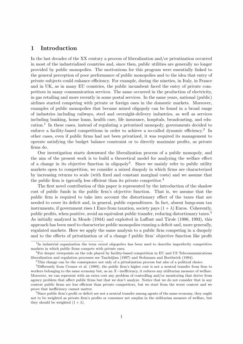
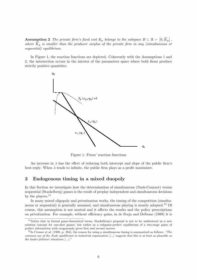
In Figure 1, the reaction functions are depicted. Coherently with the Assumptions 1 and2, the intersection occurs in the interior of the parameters space where both firms producestrictly positive quantities.
Figure 1: Firms’ reaction functions
An increase in λ has the effect of reducing both intercept and slope of the public firm’sbest-reply. When λ tends to infinite, the public firm plays as a profit maximizer.
3 Endogenous timing in a mixed duopoly
In this Section we investigate how the determination of simultaneous (Nash-Cournot) versussequential (Stackelberg) games is the result of preplay independent and simultaneous decisionsby the players.11
In many mixed oligopoly and privatization works, the timing of the competition (simulta-neous or sequential) is generally assumed, and simultaneous playing is mostly adopted.12 Ofcourse, this assumption is not neutral and it affects the results and the policy prescriptionson privatization. For example, without efficiency gains, in de Fraja and Delbono (1989) it is
11Notice that in formal game-theoretical terms, Stackelberg’s proposal is not to be understood as a newsolution concept for one-shot games, but rather as a subgame-perfect equilibrium of a two-stage game ofperfect information with exogenously given first and second movers.
12In Cremer et al. (1989, p. 284), the reason for using a simultaneous timing is summarized as follows: “Thecommon use of the Nash equilibrium in industrial organization [...] suggests that this is at least as plausible asthe leader-follower situations [...].”
6
shown that privatization never improves welfare when a Stackelberg game with public lead-ership is played; on the contrary, privatization may be welfare improving in the simultaneoussetting. Then, the welfare impact of privatization crucially depends on the assumed timing.
More recently, other works introduced the idea that the order of play should result fromthe players’ timing decision. In particular, in a private duopoly with strategic substitutabilityit has been proved by Hamilton and Slutsky (1990) and by Amir and Grilo (1999) thatsimultaneous play emerges as the unique equilibrium of the endogenous game. Conversely, ina mixed duopoly Pal (1998) shows that sequential play always occurs in equilibrium.
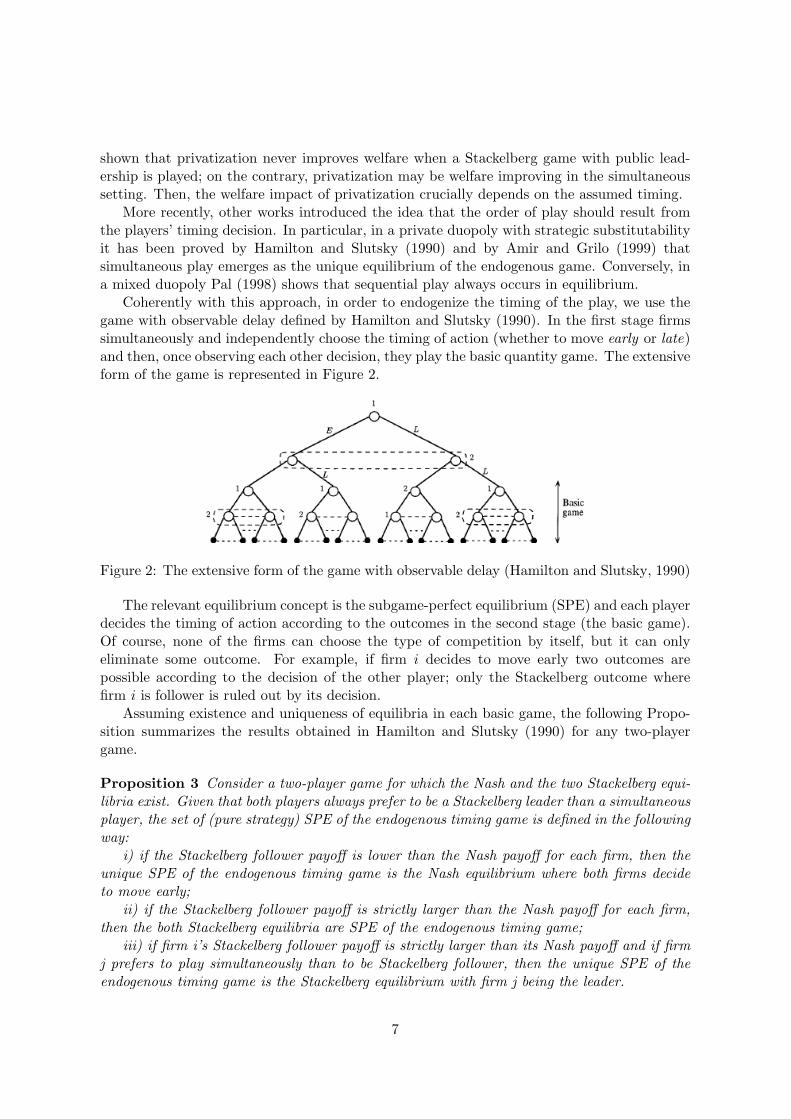
Coherently with this approach, in order to endogenize the timing of the play, we use thegame with observable delay defined by Hamilton and Slutsky (1990). In the first stage firmssimultaneously and independently choose the timing of action (whether to move early or late)and then, once observing each other decision, they play the basic quantity game. The extensiveform of the game is represented in Figure 2.
Figure 2: The extensive form of the game with observable delay (Hamilton and Slutsky, 1990)
The relevant equilibrium concept is the subgame-perfect equilibrium (SPE) and each playerdecides the timing of action according to the outcomes in the second stage (the basic game).Of course, none of the firms can choose the type of competition by itself, but it can onlyeliminate some outcome. For example, if firm i decides to move early two outcomes arepossible according to the decision of the other player; only the Stackelberg outcome wherefirm i is follower is ruled out by its decision.
Assuming existence and uniqueness of equilibria in each basic game, the following Propo-sition summarizes the results obtained in Hamilton and Slutsky (1990) for any two-playergame.
Proposition 3 Consider a two-player game for which the Nash and the two Stackelberg equi-libria exist. Given that both players always prefer to be a Stackelberg leader than a simultaneousplayer, the set of (pure strategy) SPE of the endogenous timing game is defined in the followingway:
i) if the Stackelberg follower payoff is lower than the Nash payoff for each firm, then theunique SPE of the endogenous timing game is the Nash equilibrium where both firms decideto move early;
ii) if the Stackelberg follower payoff is strictly larger than the Nash payoff for each firm,then the both Stackelberg equilibria are SPE of the endogenous timing game;
iii) if firm i’s Stackelberg follower payoff is strictly larger than its Nash payoff and if firmj prefers to play simultaneously than to be Stackelberg follower, then the unique SPE of theendogenous timing game is the Stackelberg equilibrium with firm j being the leader.
7
Proof. The proof of this Proposition follows from Theorems II, III and IV in Hamilton andSlutsky (1990).
The intuition behind these results is the following. Given that both firms prefer to beleader than to play simultaneously, if the Nash payoff is higher than the follower payoff, thenany firm has a dominant strategy to move early. But if one firm prefers its follower payoff tothe Nash payoff, there is no dominant strategy: when the other player moves early it prefersto move late and vice versa. This explains the three possible outcomes listed in Proposition3.
We use Proposition 3 in order to determine the endogenous timing equilibrium, where theexistence and the uniqueness of the equilibria in each basic game are assured by Assumptions 1and 2. The reduced form of the endogenous timing game for the mixed duopoly is representedin Table 1.
Private FirmPublic Firm Early Late
Early WMN (.), ΠMNp (.) WGL(.), ΠGL
p (.)Late WPL(.), ΠPL
p (.) WMN (.), ΠMNp (.)
Table 1: The reduced form of the endogenous timing game. MN, PL and GL stay for Nash,Private Leadership and Public Leadership equilibria respectively.
In order to solve the game we need to compare the equilibrium payoffs in each basic game.In what follows the simultaneous and sequential equilibria are derived.
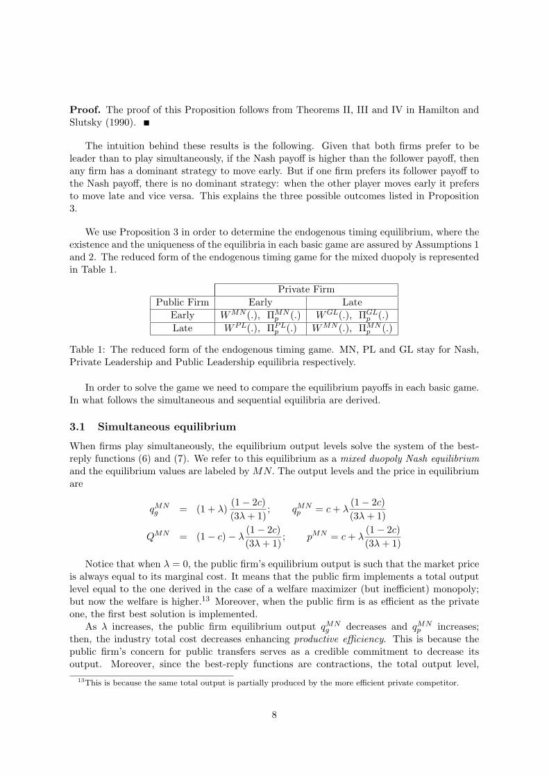
3.1 Simultaneous equilibrium
When firms play simultaneously, the equilibrium output levels solve the system of the best-reply functions (6) and (7). We refer to this equilibrium as a mixed duopoly Nash equilibriumand the equilibrium values are labeled by MN. The output levels and the price in equilibriumare
qMNg = (1 + λ)
(1− 2c)(3λ+ 1)
; qMNp = c+ λ
(1− 2c)(3λ+ 1)
QMN = (1− c)− λ (1− 2c)(3λ+ 1)
; pMN = c+ λ(1− 2c)(3λ+ 1)
Notice that when λ = 0, the public firm’s equilibrium output is such that the market priceis always equal to its marginal cost. It means that the public firm implements a total outputlevel equal to the one derived in the case of a welfare maximizer (but inefficient) monopoly;but now the welfare is higher.13 Moreover, when the public firm is as efficient as the privateone, the first best solution is implemented.
As λ increases, the public firm equilibrium output qMNg decreases and qMN
p increases;then, the industry total cost decreases enhancing productive efficiency. This is because thepublic firm’s concern for public transfers serves as a credible commitment to decrease itsoutput. Moreover, since the best-reply functions are contractions, the total output level,
13This is because the same total output is partially produced by the more efficient private competitor.
8
QMN , decreases and the market price pMN increases. It is obvious that the effect on consumersurplus is negative, raising an allocative inefficiency.14 The private firm’s profit and welfarerepresent the payoffs of the players and in the simultaneous case are:
ΠMNp =
(c+λ(1+c)
3λ+1
)2−Kp (8)
WMN = 1−2c(1+λ)(1+2λ)2+c2(1+λ)2(3+8λ)+2λ(3+λ(5+λ))
2(3λ+1)2− (1 + λ)Kg −Kp (9)
3.2 Sequential equilibria
A Stackelberg equilibrium of this game corresponds to the SPE of a two stage game of perfectinformation in which the second mover (follower) chooses an action after having observed theaction of the first mover (leader). Then, the Stackelberg equilibrium imposes that: (i) thestrategy of the second mover is a selection from its reaction function; and (ii) the first moverchooses an action that maximizes its objective given the anticipation of the rival’s reaction.
In what follows we first analyze the case of public leadership and then the private leadershipequilibrium.
Public leadership (GL).When the public firm moves before its private competitor, the equilibrium quantities solve
the following equation system:
qGLg = arg maxW (qg, rp(qg))
qGLp = rp(qGLg )
The solution is:
qGLg = max{
(1 + 2λ)− 4c (1 + λ)(1 + 4λ)
, 0}
qGLp =12(1− qGLg
)
We have to distinguish two cases since there exists a threshold value of the marginal costof the public firm such that ∀c ∈
(0, 1+2λ
4(1+λ)
)the public firm produces a positive quantity in
equilibrium. When c ∈[
1+2λ4(1+λ) ,
12
), the public firm prefers not to produce and the private
firm acts as a monopolist: its quantity, market price, and welfare are the same as in a privatemonopoly.
Since the threshold value 1+2λ4(1+λ) is increasing, as λ increases an higher level of inefficiency
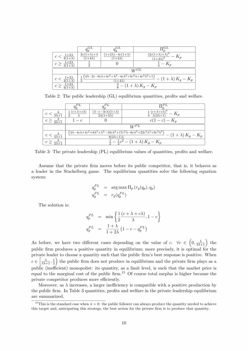
is compatible with positive production by the public firm. In Table 2 quantities, profits andwelfare in the public leadership equilibrium are summarized.
Private leadership (PL).14There exists a clear trade off between technical and allocative efficiency, and the net effect on total surplus
is ambiguous and depends on the parameters.
9
qGLp qGLg ΠGLp
c < 1+2λ4(1+λ)
2c(1+λ)+λ(1+4λ)
(1+2λ)−4c(1+λ)(1+4λ)
(2c(1+λ)+λ)2
(1+4λ)2−Kp
c ≥ 1+2λ4(1+λ)
12 0 1
4 −Kp
WGL
c < 1+2λ4(1+λ)
12
(4λ−2c−6cλ+4c2+λ2−4cλ2+8c2λ+4c2λ2+1)(1+4λ) − (1 + λ)Kg −Kp
c ≥ 1+2λ4(1+λ)
38 − (1 + λ)Kg −Kp
Table 2: The public leadership (GL) equilibrium quantities, profits and welfare.
qPLp qPLg ΠPLp
c < λ3λ+1
12
(c+λ+cλ)λ
(λ−c−3cλ)(1+λ)2λ(1+2λ)
14
(c+λ+cλ)2
λ(2λ+1) −Kp
c ≥ λ3λ+1 1− c 0 c(1− c)−Kp
WPL
c < λ3λ+1
(4λ−4cλ+4c2+8λ2+λ3−10cλ2+17c2λ−6cλ3+22c2λ2+9c2λ3)8(2λ+1)λ − (1 + λ)Kg −Kp
c ≥ λ3λ+1
12 −
12c
2 − (1 + λ)Kg −Kp
Table 3: The private leadership (PL) equilibrium values of quantities, profits and welfare.
Assume that the private firm moves before its public competitor, that is, it behaves asa leader in the Stackelberg game. The equilibrium quantities solve the following equationsystem:
qPLp = arg max Πp (rg(qp), qp)
qPLg = rg(qPLp )
The solution is:
qPLp = min{
12
(c+ λ+ cλ)λ
, 1− c}
qPLg =1 + λ
1 + 2λ(1− c− qPLp
)As before, we have two different cases depending on the value of c. ∀c ∈
(0, λ
3λ+1
)the
public firm produces a positive quantity in equilibrium; more precisely, it is optimal for theprivate leader to choose a quantity such that the public firm’s best response is positive. Whenc ∈
[λ
3λ+1 ,12
)the public firm does not produce in equilibrium and the private firm plays as a
public (inefficient) monopolist: its quantity, as a limit level, is such that the market price isequal to the marginal cost of the public firm.15 Of course total surplus is higher because theprivate competitor produces more efficiently.
Moreover, as λ increases, a larger inefficiency is compatible with a positive production bythe public firm. In Table 3 quantities, profits and welfare in the private leadership equilibriumare summarized.
15This is the standard case when λ = 0: the public follower can always produce the quantity needed to achievethis target and, anticipating this strategy, the best action for the private firm is to produce that quantity.
10
3.3 Endogenous timing equilibria
In this section we derive the endogenous timing equilibria of the mixed duopoly game. Inorder to apply Proposition 3 we need to rank the private and public firms’ payoff in thedifferent equilibria. In particular, in Lemma 4 we compare the private firm’s profit underpublic leadership (i.e., the follower payoff) and in the Nash equilibrium, while in Lemma 5 wecompare welfare under private leadership (again the follower payoff) with the one in the Nashequilibrium. It is worth noting that these comparisons are sufficient to apply Proposition 3.In fact, any player always prefers to be leader than to play simultaneously, by the nature ofStackelberg equilibria. Moreover, the comparison between the leader and the follower payoffis useless since no firm can unilaterally switch from one sequential equilibrium to the other.
Lemma 4 There exists a subspace F1 = (c,λ) ⊆ A, such that the private firm strictly prefersthe public leadership equilibrium to the mixed duopoly Nash equilibrium. In the subspace F1 =A− F1 the reverse is true.
This result totally relies on the choice of the public leader to produce more or less thanin the simultaneous equilibrium; and this choice depends on the public firm’s objective beingincreasing or decreasing in the rival’s output in the Nash equilibrium point.
In fact, private firm’s profit is strictly decreasing in the public firm’s output in any in-terior point16, and so, if qPLg < qMN
g , the private firm prefers to be follower than to playsimultaneously.
The public leader chooses to produce a smaller quantity with respect to the Nash equi-librium if ∂W (qg ,qp)
∂qp> 0 in the Nash equilibrium. In fact, if its objective is increasing in the
quantity produced by the rival, the public leader prefers to reduce its quantity anticipatingthat the private firm will increase the output, enhancing in this way the welfare.17
∂W (qg, qp)∂qp
=∂V
∂qp+ λ
∂Πg
∂qp= p (qg, qp) + λp′ (qg, qp) qg = p (qg, qp)− λqg
In the Nash equilibrium:
∂W (qg, qp)∂qp
∣∣∣∣(qMNg ,qMN
p )= c+ λ
(1− 2c)(3λ+ 1)
− λ (1 + λ)(1− 2c)(3λ+ 1)
=c(2λ2 + 3λ+ 1
)− λ2
(3λ+ 1)
Then, ∂W (qg ,qp)∂qp
∣∣∣(qMNg ,qMN
p )> 0 if c > λ2
2λ2+3λ+1.
This result occurs when the increase in productive efficiency due to the shift of someproduction to the private firms outweighs the negative allocative efficiency effect due to thereduction in total quantity and the negative distortionary effect due to the reduction in profits.
The threshold c (λ) is increasing because, as λ increases, the distortionary effect makes thepublic firm more willing to produce a larger quantity. So, only if c is high enough the overalleffect of shifting some production to the efficient private competitor is positive.
16Indeed, ∂Πp (qg, qp) /∂qg = p′ (qg, qp) qp < 0 ∀qp > 0.17Note that welfare increases despite the total quantity reduction.
11
Lemma 5 There exists a subspace F2 = (c,λ) ⊆ A, such that the public firm strictly prefersthe private leadership equilibrium to the mixed duopoly Nash equilibrium. In the subspaceF2 = A− F2 the reverse is true.
As in the previous Lemma, this result has to do with the fact that W (qg, qp) may beincreasing in qp. But now what matters is the decision of the private leader, that alwaysincreases its output with respect to the Nash equilibrium. As a result, total output increasesand the allocative efficiency effect is positive. Recalling that moving from Nash to the publicleadership equilibrium had a negative allocative efficiency effect, we would expect that theparameter space F2 is larger F1. This intuition is confirmed by the comparison of the thresholdsc (λ) and c (λ). In fact,
c (λ) =3λ2 + 7λ3
21λ+ 34λ2 + 17λ3 + 4<
λ2
2λ2 + 3λ+ 1= c (λ) ∀λ ∈
(0, λ)
Then, F1 ⊂ F2.
In the following Theorem the different SPE of the endogenous timing game are derived.
Theorem 6 Consider a mixed duopoly game in which the order of moves is endogenous. TheSPE of the endogenous timing game are defined in the following way:
a) When (c, λ) ∈ F2, the mixed duopoly Nash equilibrium is the unique SPE of the endogenoustiming game;
b) When (c, λ) ∈ F1 ∩ F2, the unique SPE of the endogenous timing game is the Stackelbergequilibrium with the private firm acting as leader;
c) When (c, λ) ∈ F1, both Stackelberg outcomes are the (pure strategy) SPE of the endogenoustiming game.
Figure 3 depicts the three possible outcomes of the endogenous timing game in the space(c, λ). Without considering λ, the previous literature (Pal, 1998) defines a unique solutionwhere both sequential equilibria are SPE. The novel contribution of our analysis is to enlargethe set of possible outcomes defining conditions under which either private leadership or Nashequilibrium may arise as the unique SPE. The intuition is straightforward. Since the publicfirm’s objective function is a weighted average of total surplus and profits, for low values ofλ (given c) our result coincides with Pal’s; for high values of λ (given c), the public firmmimics the private firm’s behaviour and we obtain the same results as Amir and Grilo (1999)in a private duopoly. For intermediate values of λ, private leadership is the unique SPE sincethe public firm is more willing to accept a reduction in its own output when total quantityincreases (in the PL equilibrium) than when total output decreases (in the GL equilibrium).
Moreover, when we focus on the sequential outcomes, the introduction of λ increases thelevel of inefficiency compatible with a strictly positive quantity produced by the public firmin equilibrium. In particular, in the private leadership case, Pal (1998) shows that the publicfirm never produces and its presence has a mere strategical role that induces the competitor toproduce the limit quantity. In our framework, taking into account the shadow cost of publicfunds, the public firm usually produces a positive quantity in equilibrium.18
18This is true as far as the public firm is not too inefficient. This result enhances the realism of our approachwhere the public firm represents not only a threat of producing, but it has an active role in the industry.
12
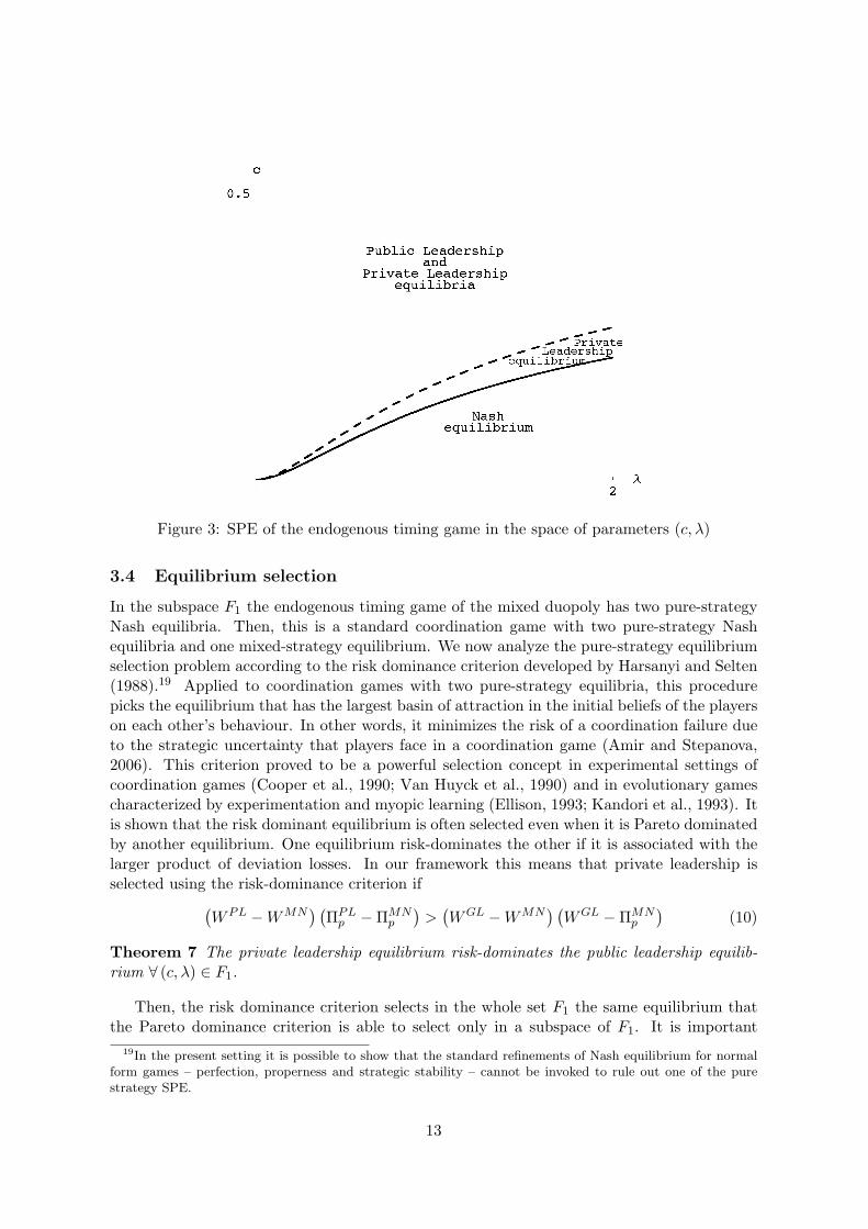
Figure 3: SPE of the endogenous timing game in the space of parameters (c, λ)
3.4 Equilibrium selection
In the subspace F1 the endogenous timing game of the mixed duopoly has two pure-strategyNash equilibria. Then, this is a standard coordination game with two pure-strategy Nashequilibria and one mixed-strategy equilibrium. We now analyze the pure-strategy equilibriumselection problem according to the risk dominance criterion developed by Harsanyi and Selten(1988).19 Applied to coordination games with two pure-strategy equilibria, this procedurepicks the equilibrium that has the largest basin of attraction in the initial beliefs of the playerson each other’s behaviour. In other words, it minimizes the risk of a coordination failure dueto the strategic uncertainty that players face in a coordination game (Amir and Stepanova,2006). This criterion proved to be a powerful selection concept in experimental settings ofcoordination games (Cooper et al., 1990; Van Huyck et al., 1990) and in evolutionary gamescharacterized by experimentation and myopic learning (Ellison, 1993; Kandori et al., 1993). Itis shown that the risk dominant equilibrium is often selected even when it is Pareto dominatedby another equilibrium. One equilibrium risk-dominates the other if it is associated with thelarger product of deviation losses. In our framework this means that private leadership isselected using the risk-dominance criterion if(
WPL −WMN) (
ΠPLp −ΠMN
p
)>(WGL −WMN
) (WGL −ΠMN
p
)(10)
Theorem 7 The private leadership equilibrium risk-dominates the public leadership equilib-rium ∀ (c, λ) ∈ F1.
Then, the risk dominance criterion selects in the whole set F1 the same equilibrium thatthe Pareto dominance criterion is able to select only in a subspace of F1. It is important
19In the present setting it is possible to show that the standard refinements of Nash equilibrium for normalform games – perfection, properness and strategic stability – cannot be invoked to rule out one of the purestrategy SPE.
13
to highlight that the risk-dominance criterion is applied to the reduced game, and not tothe entire two-stage game of endogenous timing, and the two options are a priori entirelydifferent. However, since each subgame has a unique Nash equilibrium and given the use ofsubgame perfection in this framework, our application of the risk-dominance criterion on thereduced game seems to us rather natural.20 Amir and Stepanova (2006) suggest the followinginterpretation: the private leadership equilibrium is chosen by firms that wish to minimize therisk of coordination failure in their timing decisions.
The preference for the private leadership equilibrium is the main contribution in Beatoand Mas-Colell (1984), where it is assumed that the public firm is committed to a decisionrule (in their case the marginal-cost pricing rule), and the private firm maximizes its ownprofit given the decision rule of the public competitor. In the present setting, using thegame with observable delay of Hamilton and Slutsky (1990) coupled with risk dominance as aselection criterion, we show that the private leadership equilibrium emerges as the endogenousequilibrium in the mixed duopoly ∀ (c, λ) ∈ F2.
4 Welfare effect of profit-maximizer public firm
In this Section we perform a comparative statics exercise in order to analyze the effects ofasking the public firm to directly maximize profits21 on welfare taking into account the resultof the previous Section on the endogenous timing equilibrium.
By a change in the public firm’s objective function we consider the case in which itsmanagement is instructed to maximize profits:
Πg (qg, qp) = [p (qg, qp)− c] qg
This change in the objective function might have the complementary effect of enhancing theproductive efficiency of the public firm. This can happens since it is easier to measure profitsthan to measure welfare and with the new targets public management can be monitored andmotivated in its performance. We consider the two extreme cases in which either no efficiencygain or full efficiency are achieved. In the first case, the public firm that maximize profitsretains the same technology as before; in the latter, it is able to produce at the same marginalcost of its competitor, here normalized to zero. After the objective function change, the newreaction function of firm g is:
rg(qp) = max{
12
(1− c− qp) , 0}
(11)
with c = 0 in the case of full efficiency gains. Comparing the reaction function before (7) andafter the objective function change, it is easy to see that it becomes steeper. Indeed:
1 + λ
1 + 2λ>
12
∀λ ∈(0, λ)
and only when λ→∞ the slope of (7) converges to (6).20See van Damme and Hurkens (2004) and Amir and Stepanova (2006) for the application of the risk-
dominance criterion on the reduced game of endogenous timing models in price game duopolies.21As private and privatized firm do.
14
Absent efficiency gains, also the intercept. With full efficiency gains the intercept increasesonly when c > 1
2(1+λ) .The change in the reaction function is not the only effect of asking the pubic firm to
maximize profits. In fact, we have to consider the (possible) change in the endogenous timingequilibrium. In order to derive the SPE of the game after the change, we can rely on theresults in Amir and Grilo (1999) that apply the same endogenous timing structure to a privateduopoly. The following Proposition summarizes the result.
Proposition 8 Consider a private duopoly quantity game with strategic substitutes. Whenthe values of the parameters are in the admissible set A, the unique SPE of the endogenoustiming game is the Cournot-Nash equilibrium where both firms decide to move early.
Proof of Proposition 8. Under Assumptions 1 and 2 no Nash equilibrium lies on theboundary, i.e. no firm produces zero output. In this case we can apply Theorem 2.2 inAmir and Grilo (1999) that proves that both firms prefer always to be simultaneous playerthan Stackelberg follower. So, according to point i) Proposition 3, the unique SPE of theendogenous timing game is the Cournot-Nash equilibrium.
The intuition for this result is clear. Since the firm’s profit is strictly decreasing in therival’s output, a private leader always increases its own quantity in comparison with theCournot-Nash quantity. By the same reason, a private follower is always strictly worse offwith respect to the Cournot-Nash equilibrium. Then, sequential play is only sustainable in amixed duopoly.
The Cournot-Nash equilibrium is the solution of the system of equations (6) and (11).Quantities and price are:22
qCNg =1− 2c
3; qCNp =
1 + c
3
QCN =2− c
3; pCN =
1 + c
3The (domestic) total surplus and the public firm’s profit are:
V CN =8− 8c+ 11c2
18−Kg −Kp; ΠCN
g =(
1− 2c3
)2
Recall that in the case of achieving full efficiency c = 0. Of course, in order to compare welfarebefore and after the change in the public firm’s objective function, public firm profits matter.When profits increase of 1 Euro, the measure of welfare increase of 1+λ Euros.23 In this case,total welfare in the Cournot-Nash equilibrium is:
WCN =118(2λ+ 11c2 + 8− 8c (1 + λ− cλ)
)− (1 + λ)Kg −Kp (12)
22Superscript CN stands for Cournot-Nash equilibrium.23If we extend our analysis to privatization, in order to compare welfare before and after privatization, the
price paid to the government for buying the firm matters. In fact, since we are taking into account the shadowcost of public funds, it is not indifferent whether profits are public or private, and if the government is ableto raise enough money from privatization. Given the equilibrium after privatization, the more money thegovernment is able to raise by selling the public firm, the higher the welfare after the privatization. In the firstinstance, we give full bargaining power to the government; i.e., it is able to extract the whole profit from theprivatized firm. In this case, total welfare in the Cournot-Nash equilibrium is the same computed consideringthat public firm maximizes profits, without privatization.
15
The following theorem states the result of the comparison when no efficiency gain occurs.
Theorem 9 Consider a mixed duopoly game in which the order of moves is endogenous. Inaddition, assume that by changing the objective function of the public firm no efficiency gainsare achieved. Then, maximizing profits instead of maximize welfare always reduces welfare.
This result is in sharp contrast with those obtained assuming simultaneous playing. Forexample, de Fraja and Delbono (1989) show that assuming Cournot competition privatiza-tion24 may enhance welfare absent efficiency gains.25 The same result holds in the frameworkof the present paper. Disregarding the endogenous timing game, and comparing WMN fromequation (9) and WCN from equation (12) ∀ (c, λ) ∈ A, maximizin profits (or privatization)may increase welfare. More precisely, it occurs when
c > 4λ+6λ2+126λ+12λ2+8
Now, we move the analysis to the other extreme case: full efficiency. The following Theoremformalizes the result.
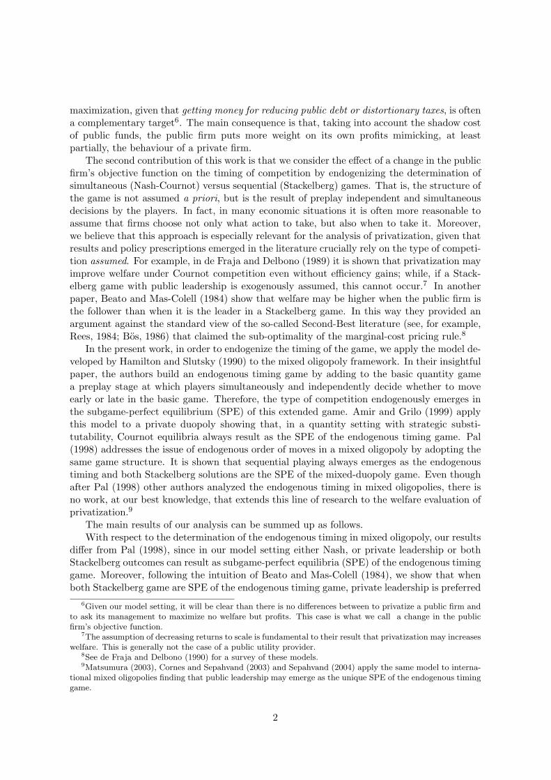
Theorem 10 Consider a mixed duopoly game in which the order of moves is endogenous. Inaddition, assume that by changing the objective function of the public firm full efficiency gainsare achieved. Then, there exists a subset of the parameter J ⊂ A, such that asking the publicfirm to maximize profits reduces welfare.
In Figure 4 we graph the set J in the parameters’ space in the case of welfare is reduced bythe change of the public firm’s objective function even if we assume to achieve full efficiency.Endogenizing the timing of competition, before and after the change of the public firm’ ob-jective function, enlarges this space with respect to the simultaneous case. In fact, it is easyto show that, assuming simultaneous competition, welfare has been reduced if
c <3(1+2λ)2−(1+3λ)
√2(3+8λ(1+λ))
3(1+λ)(3+8λ)
It is interesting to notice that the level of c such that public ownership is the dominant solutionin terms of welfare is decreasing in λ. This occurs because, as λ increases, the profit motivationhas a larger weight in the public firm’s decision.
If we extend our analysis to privatization we can notice that the allocative efficiency effectof the public ownership decreases and the productive efficiency effect of privatization becomesmore and more important. Thus, we can say that the more the public firm behaves as a profitmaximizer, the better is to privatize it. This result is obtained assuming that the governmentis able to extract the whole profit from the new owners of the privatized firm. Suppose nowthat the government is able to take just half of the profit. How the previous result are affected?In Figure 4 we can see how the space of the parameters such that the privatization reduceswelfare is enlarged. The dashed line delimits the space of a welfare-reducing full efficientprivatization when the government sells the public firm at a price equal to half of the futureprofits. An extreme result occurs when the firm is sold for free. In this latter case, a fullefficient privatization always lowers welfare.
24Recall that under our model setting, privatization and profit maximization are equivalent in terms of marketperformance.
25This result is obtained in a different setting with symmetric firms and increasing marginal costs.
16
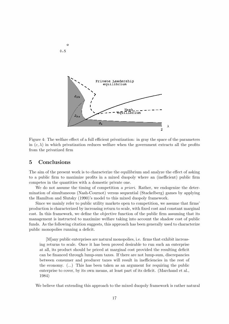
Figure 4: The welfare effect of a full efficient privatization: in gray the space of the parametersin (c, λ) in which privatization reduces welfare when the government extracts all the profitsfrom the privatized firm
5 Conclusions
The aim of the present work is to characterize the equilibrium and analyze the effect of askingto a public firm to maximize profits in a mixed duopoly where an (inefficient) public firmcompetes in the quantities with a domestic private one.
We do not assume the timing of competition a priori. Rather, we endogenize the deter-mination of simultaneous (Nash-Cournot) versus sequential (Stackelberg) games by applyingthe Hamilton and Slutsky (1990)’s model to this mixed duopoly framework.
Since we mainly refer to public utility markets open to competition, we assume that firms’production is characterized by increasing return to scale, with fixed cost and constant marginalcost. In this framework, we define the objective function of the public firm assuming that itsmanagement is instructed to maximize welfare taking into account the shadow cost of publicfunds. As the following citation suggests, this approach has been generally used to characterizepublic monopolies running a deficit.
[M]any public enterprises are natural monopolies, i.e. firms that exhibit increas-ing returns to scale. Once it has been proved desirable to run such an enterpriseat all, its product should be priced at marginal cost provided the resulting deficitcan be financed through lump-sum taxes. If there are not lump-sum, discrepanciesbetween consumer and producer taxes will result in inefficiencies in the rest ofthe economy. (...) This has been taken as an argument for requiring the publicenterprise to cover, by its own means, at least part of its deficit. (Marchand et al.,1984)
We believe that extending this approach to the mixed duopoly framework is rather natural
17
and fills, at least partially, some gaps of the previous literature. Indeed, discussing the resultsof their paper, Beato and Mas-Colell (1984, p. 82) state:
Finally, the limitations of this paper and the need for further work should beclear. We have, for example, ruled out both fixed cost and the general equilibriumeffects of distortions in other markets. We don’t know if reasonable versions of themain results of this paper [...] are available in these richer settings.
The extensive process of privatization started in the eighties of the last century and still inplace nowadays is essentially driven by the belief that private discipline and profit motivationcan enhance efficiency. Moreover, privatization is also considered as a powerful instrumentto raise money to reduce distortionary taxation. In this work we contrast the general extentof these ideas. We show that, absent efficiency gains, privatization never increases welfare,and that an inefficient public firm may be preferred even when large efficiency gains could berealized by privatization. These results are obtained assuming that both public firm’s profitsand privatization proceeds are substitute for distortionary taxation. The endogenous timingmodel applied to the mixed oligopoly framework is not less important for our results. Whileafter privatization only the simultaneous (Nash-Cournot) equilibrium can be implemented,with a public firm sequential equilibria – that are always welfare superior – may be sustained asSPE of the endogenous timing game. Therefore, privatization changes not only the ownershipand the objective function of the public firm, but also the type of competition in the market.
Finally, the assumption of larger marginal cost for the public firm deserves a last comment.In our model we follow the general presumption that public ownership is relatively inefficientwhen compared to private ownership. This has been justified by the theory of incentivesthat has been used to demonstrate that agency problems in state-owned enterprises can causelarger inefficiencies than in private-owned firms. But we are aware that from an empiricalpoint of view the picture is quite mixed and the variance of the results substantial (Cuervoand Villalonga, 2000).26 However, any relaxation of our assumption obviously strengthen theresults obtained in this paper.
6 Appendix
Proof of Lemma 4. Comparing the equilibrium profits ΠGLp in Table 2 with ΠMN
p inequation (8), it easy to check that ∀λ ≥ 0:
(i) ∀c ∈(
0, 1+2λ4(1+λ)
)ΠGLp −ΠMN
p > 0 ∀c > c (λ)
where
c (λ) =λ2
2λ2 + 3λ+ 1with
∂c (λ)∂λ
> 0.
26See for example the reviews of Megginson and Netter (2001) and Willner (2001) that report the resultsof hundreds of empirical papers on privatization and on the comparison of private and public ownership, andNewbery (2000, chapter 3) that summarizes empirical findings on the technical and economic efficiency ofprivate and public firms in utility markets.
18
(ii) ∀c ∈[
1+2λ4(1+λ) ,
12
), ΠGL
p −ΠMNp > 0 always.
Thus, we define the subspace F1 and F1 as follows:
F1 = {(c, λ) ⊆ A|c > c (λ)} and F1 = {(c, λ) ⊆ A|c ≤ c (λ)} (13)
Proof of Lemma 5. Comparing the welfare level WPL in Table 3 with WMN in equation(9), it easy to check that ∀λ ∈
(λ):27
(i) ∀c ∈(
0, λ3λ+1
)WPL −WMN > 0 ∀c > c (λ)
where
c (λ) =3λ2 + 7λ3
21λ+ 34λ2 + 17λ3 + 4with
∂c (λ)∂λ
> 0
(ii) ∀c ∈[
λ3λ+1 ,
12
),
WPL −WMN > 0 ∀λ ∈(0, λ)
Thus, we define the subspace F2 and F2 as follows:
F2 = {(c, λ) ⊆ A|c > c (λ)} and F2 = {(c, λ) ⊆ A|c ≤ c (λ)} (14)
Proof of Theorem 6.
a) When (c, λ) ∈ F1 the private firm prefers the mixed duopoly Nash equilibrium to thepublic leadership equilibrium. When (c, λ) ∈ F2 the public firm is better off in the Nashequilibrium than in the private leadership equilibrium. Therefore, in the intersectionspace F1 ∩ F2, no firm wants to be follower. Since ∀λ ∈
(0, λ), c (λ) < c (λ), it follows
that F2 ⊂ F1; then F1 ∩ F2 coincides with F2. Given that each player always prefers tobe the Stackelberg leader than a simultaneous player, point i) of Proposition 3 appliesand the mixed duopoly Nash equilibrium is the unique SPE of the endogenous timinggame.
b) When (c, λ) ∈ F1 the private firm prefers the mixed duopoly Nash equilibrium to thepublic leadership equilibrium. When (c, λ) ∈ F2 the public firm is better off in theprivate leadership equilibrium than in the mixed duopoly Nash equilibrium. So, pointiii) of Proposition 3 applies and the Stackelberg equilibrium with the private firm actingas leader is the unique SPE of the endogenous timing game.
27The threshold c < λ3λ+1
∀λ < 5.37228. Since λ is a measure of the distortion by taxation, we are comfortable
assuming that λ is lower than 5.37228. If λ ≥ 5.37228 we would have that WPL < WMN always.
19
c) When (c, λ) ∈ F1 the private firm prefers to play as Stackelberg follower than to playsimultaneously. When (c, λ) ∈ F2 the public firm prefers to play as Stackelberg followerthan to play simultaneously. Since∀λ > 0, c (λ) < c (λ), it follows that F1 ⊂ F2; thenF1 ∩ F2 coincides with F1. So, point ii) of Proposition 3 applies and both Stackelbergequilibria belong to the set of the (pure strategy) SPE of the endogenous timing game.
Proof of Theorem 7. In order to prove the result we need to consider three cases dependingon the fact that boundary solutions may occur in the two sequential equilibria. By comparingthe thresholds defined in Section 3.2, we have the following equilibria:
(i) when (c, λ) ∈ F1 and c < λ1+3λ , both Stackelberg equilibria are interior. Then, the values
of WGL, ΠGLp , WPLand ΠPL
p of interest are those in the first row of Tables 2 and 3.
(ii) when (c, λ) ∈ F1 and λ1+3λ < c < 1+2λ
4(1+λ) , the public firm does not produce in the pri-vate leadership equilibrium while it produces positive quantity in the public leadershipequilibrium. Then, the values of WGL and ΠGL
p of interest are are those in the first rowof Table 2, while for WPLand ΠPL
p we have to consider the values in the second row ofTable 3.
(iii) when (c, λ) ∈ F1 and c > 1+2λ4(1+λ) , the public firm does not produce in both Stackelberg
equilibria. Then, the values of WGL, ΠGLp , WPLand ΠPL
p of interest are those in thesecond row of Tables 2 and 3.
Applying the criterion (10), straightforward but tedious computations show the result.
Proof of Theorem 9. In order to prove the result, we need to consider three cases: (i)Nash is the relevant equilibrium of the mixed duopoly; (ii) private leadership is the relevantequilibrium of the mixed duopoly with an interior solution;and (iii) private leadership withthe public firm not producing is the relevant equilibrium of the mixed duopoly.
(i) By point a) in Theorem 6 Nash is the relevant equilibrium of the mixed duopoly gamewhen (c, λ) ∈ F2. So, we have to compare WMN , defined in equation (9) with WCN
(equation 12). Straightforward computations show that
WMN > WCN ∀ (c, λ) ∈ F2
(ii) By points b) and c) in Theorem 6 and Theorem 7 the Stackelberg outcome with theprivate firm as leader is the relevant SPE of the mixed duopoly game when (c, λ) ∈ F2.Moreover, when c < λ
3λ+1 the public firm produces positive quantity in the equilibrium.Then, we have to compare the value of WPL in the first row of Table 3 with WCN
(equation 12). Straightforward computations show that
WPL > WCN ∀ (c, λ) ∈ F2, c <λ
3λ+ 1
20
(iii) When c ≥ λ3λ+1 , the public firm does not produce in the private leadership equilibrium.
Thus, we have to compare the value of WPL in the second row of Table 3 with WCN
(equation 12). Straightforward computations show that
WPL > WCN ∀ (c, λ) ∈ F2, c >λ
3λ+ 1
Proof of Theorem 10. When the privatized firm achieves full efficiency gains, welfare afterprivatization is:
WCN∣∣c=0
=4 + λ
9− (1 + λ)Kg −Kp (15)
In order to prove the result we have to distinguish between three cases as in Theorem 9.
(i) By point a) in Theorem 6 Nash is the relevant equilibrium of the mixed duopoly gamewhen (c, λ) ∈ F2. So, we have to compare WMN , defined in equation (9) with WCN
(equation 15). Straightforward computations show that
WMN ≥ WCN∣∣c=0
∀ (c, λ) ∈ F2, c <3(1+2λ)2−(1+3λ)
√2(3+8λ(1+λ))
3(1+λ)(3+8λ)
Thus, we can define the subset
J1 ={
(c, λ) ∈ F2
∣∣∣ c < 3(1+2λ)2−(1+3λ)√
2(3+8λ(1+λ))
3(1+λ)(3+8λ)
}Referring to the definition of the subset F2 in (14), it is easy to check that J1 is anonempty set.
(ii) By points b) and c) in Theorem 6 and Theorem 7 the private leadership equilibrium is therelevant SPE of the mixed duopoly game when (c, λ) ∈ F2. Moreover, when c < λ
3λ+1the public firm produces positive quantity in the equilibrium. Then, we have to comparethe value of WPL in the first row of Table 3 with WCN (equation 15). First of all, define
F2a ={
(c, λ) ∈ F2|c <λ
3λ+ 1
}Straightforward computations show that:
WPL ≥ WCN∣∣c=0
∀ (c, λ) ∈ F2a, 9c2 (1 + λ)2 (4 + 9λ)− 18cλ (1 + λ) (2 + 3λ) + 4λ− 7λ3 > 0
Thus we can define the subset
J2a ={
(c, λ) ∈ F2a| 9c2 (1 + λ)2 (4 + 9λ)− 18cλ (1 + λ) (2 + 3λ) + 4λ− 7λ3 > 0}
that is nonempty.
21
(iii) Defining
F2b ={
(c, λ) ∈ F2|c ≥λ
3λ+ 1
}the public firm does not produce in the private leadership equilibrium. Then, we haveto compare the value of WPL in the second row of Table 3 with WCN (equation 15).Straightforward computations show that the subset J2b ⊂ F2b such that privatizationreduces welfare is not empty.
J2b ={
(c, λ) ∈ F2b|c <13
√1− 2λ⇔WPrL −WFE ≥ 0
}Then, the subset of parameters’ values such that a full efficient privatization with full
bargaining power to the government reduces welfare is the following:
J = J1 ∪ J2a ∪ J2b
References
Amir, Rabah and Anna Stepanova, “Second-mover advantage and price leadership inBertrand duopoly,” Games and Economic Behavior, April 2006, 55 (1), 1–20.
and Isabel Grilo, “Stackelberg versus Cournot Equilibrium,” Games and Economic Be-havior, January 1999, 26 (1), 1–21.
Beato, Paulina and Andreu Mas-Colell, “The Marginal Cost Pricing Rule as a RegulationMechanism in Mixed Markets,” in Maurice Marchand, Pierre Pestieu, and Henry Tulkens,eds., The Performance of Public Enterprises, North-Holland, Amsterdam, 1984.
Bos, Dieter, Public Enterprise Economics: Theory and Applications, Vol. 23 of AdvancedTextbooks in Economics, Amsterdam & New York: North Holland, 1986.
Cooper, Russell W., Douglas V. DeJong, Robert Forsthe, and Thomas W. Ross,“Selection criteria in coordination games: Some experimental results,” American EconomicReview, March 1990, 80 (1), 218–233.
Cornes, Richard C. and Mehrdad Sepahvand, “Cournot Vs Stackelberg Equilibria witha Public Enterprise and International Competition,” Working Paper Series, SSRN 2003.
Cremer, Helmuth, Maurice Marchand, and Jacques-Francois Thisse, “The PublicFirm as an Instrument for Regulating an Oligopolistic Market,” Oxford Economic Papers,April 1989, 41 (2), 283–301.
Cuervo, Alvaro and Belen Villalonga, “Explaining the Variance in the PerformanceEffects of Privatization,” Academy of Management Review, July 2000, 25 (3), 581–590.
de Fraja, Giovanni and Flavio Delbono, “Alternative Strategies of a Public Enterprisein Oligopoly,” Oxford Economic Papers, April 1989, 41 (2), 302–311.
22
and , “Game Theoretic Models of Mixed Oligopoly,” Journal of Economic Surveys, 1990,4 (1), 1–17.
Ellison, Glenn, “Learning, Local Interaction, and Coordination,” Econometrica, September1993, 61 (5), 1047–1071.
Fjell, Kenneth and Debashis Pal, “A mixed oligopoly in the presence of foreign privatefirms,” Canadian Journal of Economics, August 1996, 29 (3), 737–743.
Hamilton, Jonathan H. and Steven M. Slutsky, “Endogenous timing in duopoly games:Stackelberg or cournot equilibria,” Games and Economic Behavior, March 1990, 2 (1), 29–46.
Harsanyi, John C. and Reinhard Selten, A General Theory of Equilibrium Selection inGames, Cambridge, MA: The MIT Press, June 1988.
Hindriks, Jean and Denis Claude, “Strategic Privatization and Regulation Policy inMixed Markets,” The Icfai Journal of Managerial Economics, February 2006, 2 (4), 7–26.
Kandori, Michihiro, George J. Mailath, and Rafael Rob, “Learning, Mutation, andLong Run Equilibria in Games,” Econometrica, January 1993, 61 (1), 29–56.
Laffont, Jean-Jacques and Jean Tirole, “Using Cost Observation to Regulate Firms,”Journal of Political Economy, June 1986, 94 (3), 614–641.
and , A Theory of Incentives in Procurement Regulation, Cambridge, MA: MIT Press,1993.
Marchand, Maurice, Pierre Pestieu, and Henry Tulkens, “The Performance of Pub-lic Enterprises: Normative, Positive and Empirical Issues,” in Maurice Marchand, PierrePestieu, and Henry Tulkens, eds., The Performance of Public Enterprises, Vol. 33 of Stud-ies in Mathematical and Managerial Economics, Amsterdam, NL: Elsevier Science B.V.,January 1984, pp. 3–42.
Martin, Steven, “Globalization and the Natural Limits of Competition,” in Manfred Neu-mann and Jurgen Weigand, eds., The International Handbook of Competition, Cheltenham,UK: Edward Elgar, 2004.
Matsumura, Toshihiro, “Partial privatization in mixed duopoly,” Journal of Public Eco-nomics, December 1998, 70 (3), 473–483.
, “Stackelberg Mixed Duopoly with a Foreign Competitor,” Bulletin of Economic Research,2003, 55 (3), 275–287.
Meade, J. E., “Price and Output Policy of State Enterprise,” The Economic Journal, De-cember 1944, 54 (215/216), 321–339.
Megginson, William L. and Jeffry M. Netter, “From State to Market: A Survey ofEmpirical Studies on Privatization,” Journal of Economic Literature, June 2001, 39 (2),321–389.
Newbery, David M., Privatization, Restructuring, and Regulation of Network UtilitiesWalras-Pareto Lectures, Cambridge, MA: The MIT Press, May 2000.
23
Pal, Debashis, “Endogenous timing in a mixed oligopoly,” Economics Letters, November1998, 61 (2), 181–185.
and Mark D. White, “Mixed Oligopoly, Privatization, and Strategic Trade Policy,”Southern Economic Journal, October 1998, 65 (2), 264–281.
Rees, Ray, Public Enterprise Economics, 2nd ed., London: Weidenfeld and Nicolson, 1984.
Sepahvand, Mehrdad, “Public Enterprise Strategies in a Market Open to Domestic andInternational Competition.,” Annales d’Economie et de Statistique, 2004, 75–76, 135–153.
Stehmann, Oliver and Rob Borthwick, “Infrastructure competition and the EuropeanUnion’s telecommunications policy,” Telecommunications Policy, November 1994, 18 (8),601–615.
Taschdjian, Martin, “Alternative Models of Telecommunications Policy: Services Compe-tition versus Infrastructure Competition,” in “Twenty-Fifth Annual TelecommunicationsPolicy Research Conference” Alexandria 1997.
van Damme, Eric and Sjaak Hurkens, “Endogenous price leadership,” Games and Eco-nomic Behavior, May 2004, 47 (2), 404–420.
Van Huyck, John B., Raymond C. Battalio, and Richard O. Beil, “Tacit coordinationgames, strategic uncertainty, and coordination failure,” American Economic Review, March1990, 80 (1), 234–248.
Willner, Johan, “Ownership, efficiency, and political interference,” European Journal ofPolitical Economy, November 2001, 17 (4), 723–748.
24