pareto optimal allocation and price equilibrium for a duopoly with negative externality
TRANSCRIPT
Annals of Operations Research 116, 129–152, 2002 2002 Kluwer Academic Publishers. Manufactured in The Netherlands.
Pareto Optimal Allocation and Price Equilibriumfor a Duopoly with Negative Externality ∗
PABLO DORTA-GONZÁLEZ∗∗, DOLORES-ROSA SANTOS-PEÑATE and RAFAEL SUÁ[email protected]
Departamento de Métodos Cuantitativos en Economía y Gestión,Facultad de Ciencias Económicas y Empresariales, Universidad de Las Palmas de Gran Canaria,Campus de Tafira, 35017 Las Palmas de Gran Canaria, Spain
Abstract. A spatial competition model involving decisions made by consumers and firms is proposed.A regulating agent assigns the demand, taking into account the price, transport and externality cost, andminimizing the joint consumer cost to obtain a Pareto optimal allocation. Assuming the Pareto optimalallocation, firms fix prices in order to maximize the profit. An equilibrium problem is studied and someresults are presented. The problem and results are illustrated with an example.
Keywords: duopoly, prices, externality, equilibrium
Introduction
Spatial competition is an important field of investigation in Industrial Organization, Re-gional Science and Operation Research. In general, models involve decisions on lo-cation, price and production, made by firms in a spatial market. The model of “com-petition in quantities” presented by Cournot in 1838 is considered the first study onduopoly. Later, in 1883, Bertrand introduced “competition in prices” as an alternativeto Cournot’s model. Price and location were first combined by Hotelling [11] who pro-posed a competitive location model on a linear market in which the demand is uniformlydistributed.
Equilibrium problems in spatial competition on a network considering locationand price or production, have been studied by Lederer and Thisse [15], Labbé andHakimi [13], and Sarkar, Gupta and Pal [17], among others. Equilibrium models incor-porating location and externality cost have been investigated by Brandeau and Chiu [1,2].
In this paper, a competitive location problem on a network, considering the locationof the firms, the allocation of the demand and prices, is formulated. The goods areassumed to be essential, this means that the demand is perfectly inelastic. The modelinvolves the transport cost, the price of goods and negative externality costs. A regulatingagent assigns the demand to the firms in order to achieve a Pareto optimal allocation, andthe firms fix price maximizing profits. Assuming the Pareto optimal allocation, the price
∗ Partially financed by Gobierno de Canarias PI 2000/057.∗∗ Corresponding author.
130 DORTA-GONZÁLEZ ET AL.
equilibrium is investigated. The location equilibrium is not included in this paper andwill be analyzed in future work.
The social objective, consisting of minimizing the users’ joint cost has interest incertain public services such as health, education, and in the area of collection and treat-ment of waste. An example is found in the public health system where the public healthadministration uses private health centers in order to reduce waiting lists and make pub-lic hospitals less crowded. This is the case, for example, of some surgery, post-surgeryand hemodialysis services offered to the population by the Servicio Canario de Saludwhich determines the public health policy in the Canary Islands (Spain) and financesthese services. It is reasonable to consider that the public administration allocates ser-vices in order to minimize the total cost consisting of the transport cost, the externalitycost (e.g., a cost associated to the waiting time to be attended) and the service cost.
Another scenario where the social objective is present is related to the collectionand treatment of waste. In recent years, the problems produced by pollution and theelimination of waste have become of great importance. The European laws oblige themember countries to eliminate solid urban waste materials, heavily penalizing those thatdo not carry out certain quotas (depending on the type of residue). In order to satisfythe legal requirements, the local and regional administrations plan actions in a coordi-nated way, and some operations such as the transportation of waste and the managementof treatment plants are commissioned to private enterprises and financed by the publicadministration. In this case, the total cost includes the transportation cost, the treatmentcost, and an externality cost associated to the quantity of waste to be processed at anyone of the treatment plants.
The situations above have motivated the model presented in this paper. Moreover,it is possible to establish a relationship between the Pareto optimal allocation and theuser-choice equilibrium characterized by Brandeau and Chiu [1,2]. In fact, the Paretooptimal solution for the externality functions Ei(q) is the user-choice equilibrium whenthe externality functions are Qi(q) = Ei(q) + qE′
i (q) = ddq (qEi(q)), where index i
denotes firm i.The rest of the paper is organized as follows. In section 2, the notation and the
model are introduced. The Pareto optimal allocation and the price equilibrium are dis-cussed in section 3. Section 4 contains an example illustrating the model. Finally, someconcluding remarks are presented in section 5.
1. Notation and model
Let N(V,E) be an undirected connected network with node set V and edge set E. Twofirms, A and B, located on the network at points xA and xB , respectively, provide aproduct to consumers at nodes vk ∈ V , k = 1, 2, . . . , n. The demand at node vk is λk
and the total demand is � = ∑nk=1 λk. The demand is perfectly inelastic and it is totally
satisfied, therefore � = �A + �B where �i is the market share captured by firm i,i = A,B. The marginal cost for firm i is assumed to be independent of the quantitysupplied and it is denoted by Ci .
PARETO OPTIMAL ALLOCATION 131
Consider the following notation:
– λi = (λ1i , . . . , λni), i = A,B, and λki � 0 is the allocation of node k to firm i
(λk = λkA + λkB and �i = ∑nk=1 λki);
– tki = t (d(vk, xi)) is the unit transport cost from the demand node k to the firm locatedat xi ; this cost is an increasing function of the distance;
– pi is the unit mill price determined by firm i;
– Ei(�i) is the unit externality cost of firm i, i = A,B.
The externality is a positive, increasing and convex function of the demand cap-tured. Note that, as �A = � − �B , EA (EB ) is a decreasing function of �B (�A).
There is an allocation system which assigns the demand to firms minimizing thejoint cost, given by
Cost(pA, pB,λA,λB) =n∑
k=1
Costk(pA, pB, λkA, λkB),
with
Costk(pA, pB, λkA, λkB) =∑
i=A,B
λki
(pi + tki + Ei(�i)
).
Firm i decides the price pi that maximizes the profit, taking into account thatconsumers minimize the joint cost in order to obtain a Pareto optimum allocation(i = A,B).
The profit functions are
πA(pA, pB)= (pA − CA)�A(pA, pB) − FA,
πB(pA, pB)= (pB − CB)�B(pA, pB) − FB,
where Fi , i = A,B, are the fixed costs.
2. Equilibrium analysis
In this section the Pareto optimal allocation and the price equilibrium are studied. In thestudy of the price equilibrium, the externality cost functions are assumed to be linear.This assumption gives a model which can be considered unrealistic and too simple, how-ever, it is a way of obtaining results without leading to intractable problems (see [14]).
2.1. The Pareto optimal allocation
Suppose a regulator assigns the demand to obtain a Pareto optimum allocation (mini-mizing the joint cost). Given the prices pA and pB , the joint cost function is
Cost(λA,λB) =n∑
k=1
Costk(λkA, λkB).
132 DORTA-GONZÁLEZ ET AL.
The regulator wants to obtain a Pareto optimum allocation, that is, to solve thefollowing problem,
min Cost(λA,λB)
s.t. λk = λkA + λkB, k = 1, . . . , n,
λkA, λkB � 0, k = 1, . . . , n.
Replacing λkB by λk − λkA and considering that � = �A + �B, the objectivefunction can be written as
Cost(λA) =n∑
k=1
{λkA
(pA + tkA + EA(�A)
)+ (λk − λkA)(pB + tkB + EB(� − �A)
)},
and the resulting allocation problem is
min Cost(λA)
s.t. 0 � λkA � λk, k = 1, . . . , n.
Lemma 1. If the function f : �0+ → � is positive, increasing and convex, then thefunction g : �0+ → � defined as g(x) = xf (x) is strictly convex on �0+ = {x ∈ �:x � 0}.
Lemma 2. If Ei , i = A,B, are positive, increasing and convex, then the functionCost(λA) is strictly convex.
Proof. Note that
Cost(λA)=n∑
k=1
{λkA(pA + tkA) + (λk − λkA)(pB + tkB)
}+ �AEA(�A) + (� − �A)EB(� − �A)
is the sum of F(λA) = �AEA(�A), G(λA) = (� − �A)EB(� − �A), and a linearfunction. Moreover, F(λA) = (g ◦ f )(λA) with f : �n → �, f (λA) = ∑n
k=1 λkA, andg : � → �, g(x) = xEA(x). The function f is linear and, by lemma 1, the function g
is strictly convex, therefore g ◦ f is strictly convex. Similarly, it follows that G is alsostrictly convex. Since Cost is the sum of convex and strictly convex functions, Cost isstrictly convex. �
Proposition 1. If Ei , i = A,B, are positive, increasing and convex, then the allocationproblem min Cost(λA) subject to 0 � λkA � λk, k = 1, . . . , n, has a unique optimalsolution and the optimum is global.
Proof. The result follows from the convexity of the optimization problem and from thestrict convexity of the objective function. �
PARETO OPTIMAL ALLOCATION 133
Notice that, under the previous assumptions, the optimal market share is unique.In order to obtain its expression, the following notation is introduced. Let
�k = tkB + pB − tkA − pA, k = 1, 2, . . . , n,
�0 = +∞, �n+1 = −∞.
Without loss of generality, assume that
�1 > �2 > · · · > �n−1 > �n.
If �k = �k+1 then the demand nodes k and k + 1 are aggregated. We also define
fj =j∑
k=1
λk, j = 1, 2, . . . , n, f0 = 0.
The following result gives the Pareto optimal allocation as a function of the marketshare.
Proposition 2. Let Ei , i = A,B, be positive, increasing and convex. If q̄ = �̄A isthe Pareto optimal market share for the firm A (�̄B = � − q̄), then there exists j ∈{1, 2, . . . , n} such that fj−1 � q̄ � fj and the Pareto optimal allocations, λ̄A and λ̄B ,are
λ̄kA = λk if 1 � k � j − 1,
λ̄jA = q̄ − fj−1,
λ̄kA = 0 if k > j,
λ̄kB = λk − λ̄kA, k = 1, 2, . . . , n.
Proof. Since q̄ ∈ [0,�] and {fj }nj=0 is a partition of [0,�], there exists j ∈{1, 2, . . . , n} such that q̄ ∈ [fj−1, fj ]. Suppose that λ0
A = (λ01A, λ
02A, . . . , λ
0nA) is
an optimal allocation and λ̄A �= λ0A. Since λ̄A �= λ0
A there exists r ∈ {1, . . . , j}and s ∈ {j, . . . , n}, r < s, such that λ̄rA > λ0
rA and λ̄sB > λ0sB . Let α =
min{λ̄rA−λ0rA, λ̄sB −λ0
sB} and consider the allocation λ1A such that λ1
kA = λ0kA, ∀k �= r, s,
λ1rA = λ0
rA + α, λ1sA = λ0
sA − α. Let Cost0 and Cost1 be the costs for the allocations λ0A
and λ1A, respectively. Then
Cost1 = Cost0 + α(�s − �r) < Cost0.
From the above inequality it follows that λ0A is not optimal. �
Proposition 3. Let Ei , i = A,B, be positive, increasing and convex, and the totalexternality cost
TEC(q) = qEA(q) + (� − q)EB(� − q),
d
dx
(g(x)
)∣∣∣∣x0
= g′(x0).
134 DORTA-GONZÁLEZ ET AL.
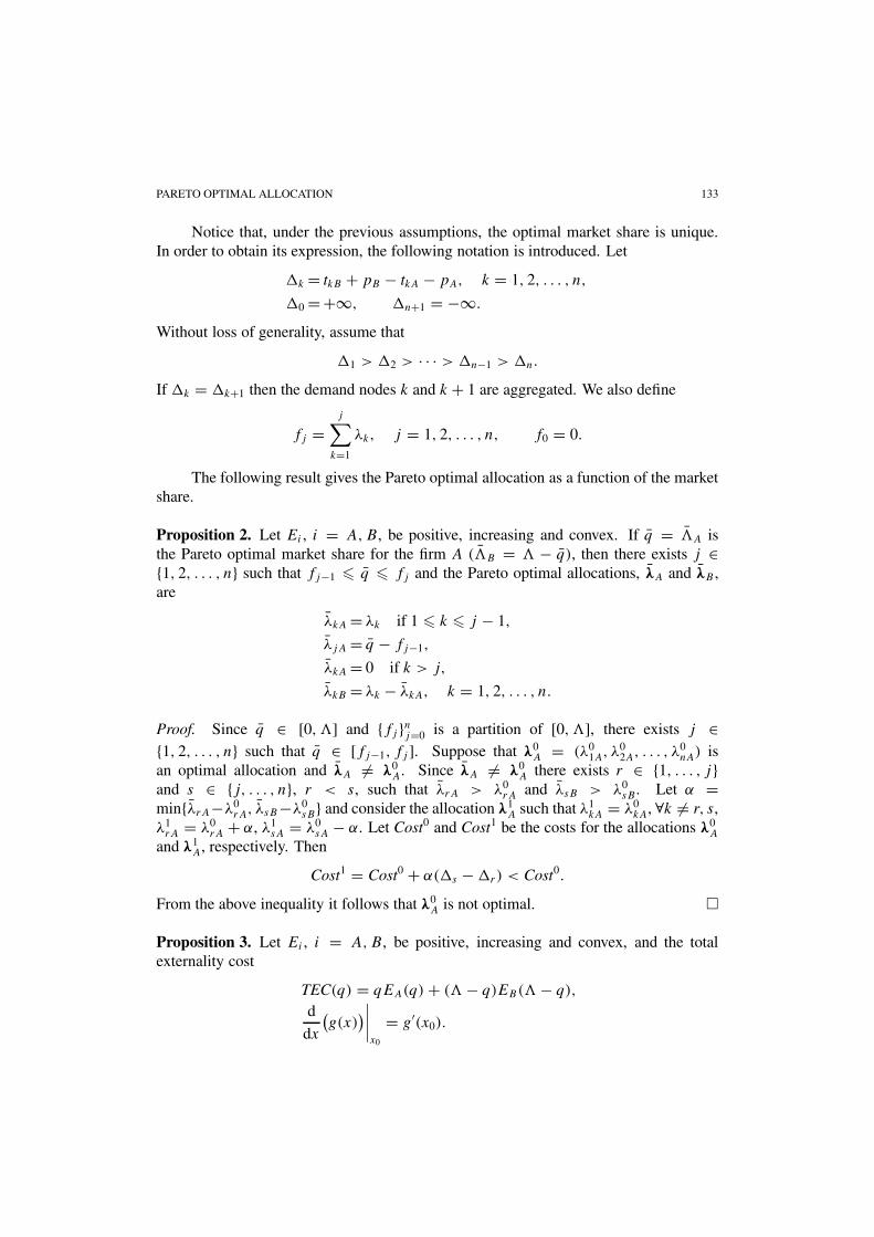
Figure 1. Pareto optimal market share.
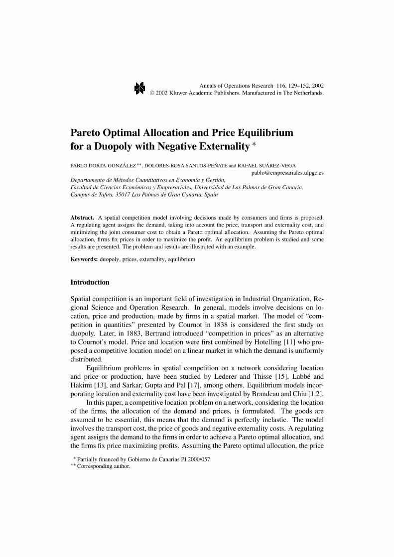
Then, the Pareto optimal market share for the firm A is
q̄ = fj if �j+1 � d
dq
(TEC(q)
)∣∣∣∣fj
� �j with j ∈ {0, 1, . . . , n} ,
fj−1 < q̄ < fj ifd
dq
(TEC(q)
)∣∣∣∣q̄
= �j with j ∈ {1, . . . , n}.
Proof. See proof in appendix A. �
Figure 1 illustrates the above result. Notice that the optimal market share is unique.It is possible to establish a relation between the Pareto optimal allocation and the
concept of user-choice equilibrium used by Brandeau and Chiu [1,2]. According toBrandeau and Chiu, a user-choice pattern {λki}k,i is a user-choice equilibrium and {�i}iis the equilibrium facility utilization if tkj + Ej(�j) � tki + Ei(�i), ∀i.
Moreover, the user-choice equilibrium is the solution of the following optimizationproblem
min∑k
∑i
λkitki +∑
i
Gi(�i)
s.t.∑
i
λki = λk, ∀k,
λki � 0, ∀k,∀i,where �i = ∑
k λki and Gi(�i) = ∫ �i
0 Ei(q) dq.This problem has the same structure as a traffic equilibrium problem. The functions
Gi are strictly convex since each Ei is positive and increasing. If Ei(q) is replaced byQi(q) = d
dq (qEi(q)) = Ei(q) + qE′i (q), then the user-choice equilibrium problem
is the Pareto optimal allocation problem when the externality cost functions are Ei(q).If Ei(q) = eiq, ∀i, the Pareto optimal allocation gives a user-choice equilibrium forQi(q) = 2eiq = 2Ei(q).
PARETO OPTIMAL ALLOCATION 135
2.2. Price equilibrium with linear externalities
In the remainder of this paper linear externality functions are considered and, assumingthe Pareto optimal allocation, the price equilibrium is obtained. Let Ei(q) = eiq, ei > 0,i = A,B. We can then state the following result.
Corollary 1. If Ei(q) = eiq, ei > 0, i = A,B, and
Lj = tjB − tjA + 2eB� − 2(eA + eB)fj , j = 1, . . . , n,
Tj−1 = tjB − tjA + 2eB� − 2(eA + eB)fj−1, j = 1, . . . , n,
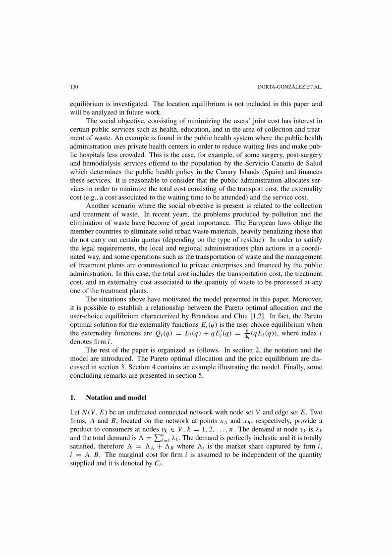
then the optimal market share is
�̄A =
� if pA − pB � Ln,pB − pA + tjB − tjA + 2eB�
2(eA + eB)if Lj < pA − pB < Tj−1, j = 1, . . . , n,
fj if Tj � pA − pB � Lj , j = 1, . . . , n − 1,0 if pA − pB � T0
and �̄B = � − �̄A.
Proof. From proposition 3 it follows that
�̄A =
fj if�j+1 + 2eB�
2(eA + eB)� fj � �j + 2eB�
2(eA + eB)with j ∈ {0, 1, . . . , n},
�j + 2eB�
2(eA + eB)if fj−1 <
�j + 2eB�
2(eA + eB)< fj with j ∈ {1, . . . , n},
which is equivalent to the expression in corollary 1. �
Notice that
Ln < Tn−1 < Ln−1 < · · · < Tj < Lj < Tj−1 < Lj−1 < · · · < T1 < L1 < T0.
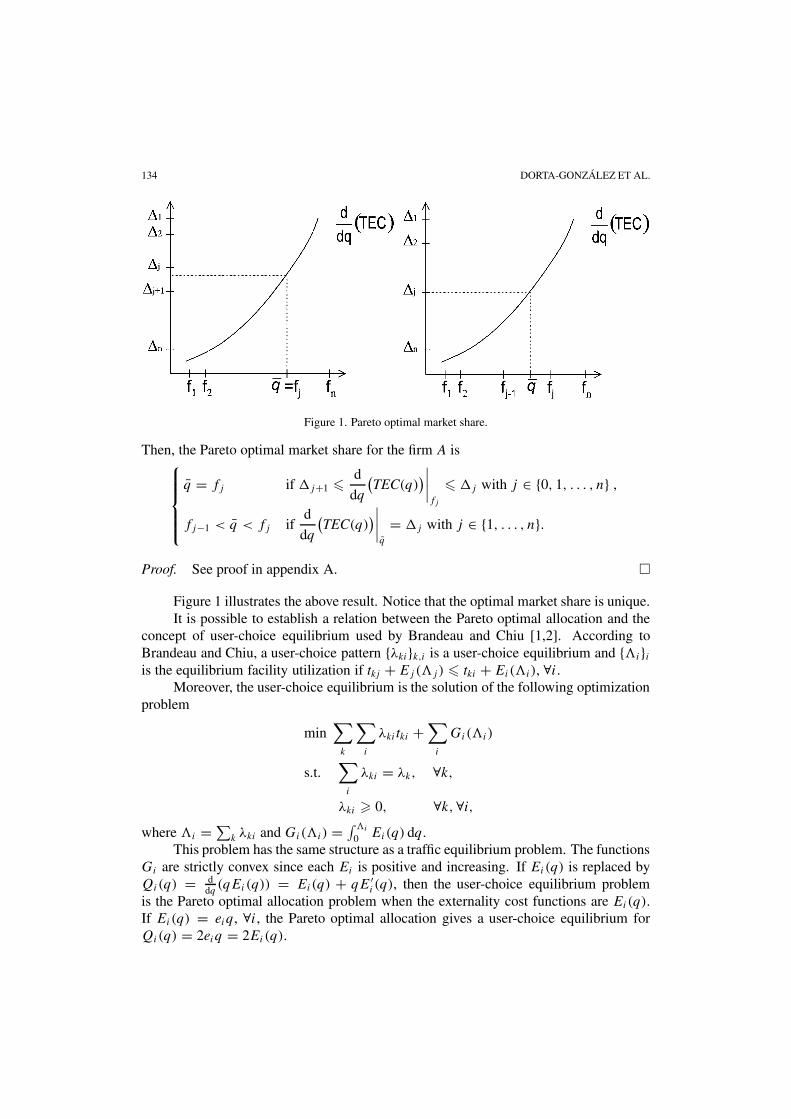
Moreover, �̄A and �̄B are continuous functions of (pA, pB) and therefore the profitfunctions are also continuous. Figure 2 shows the market shares.
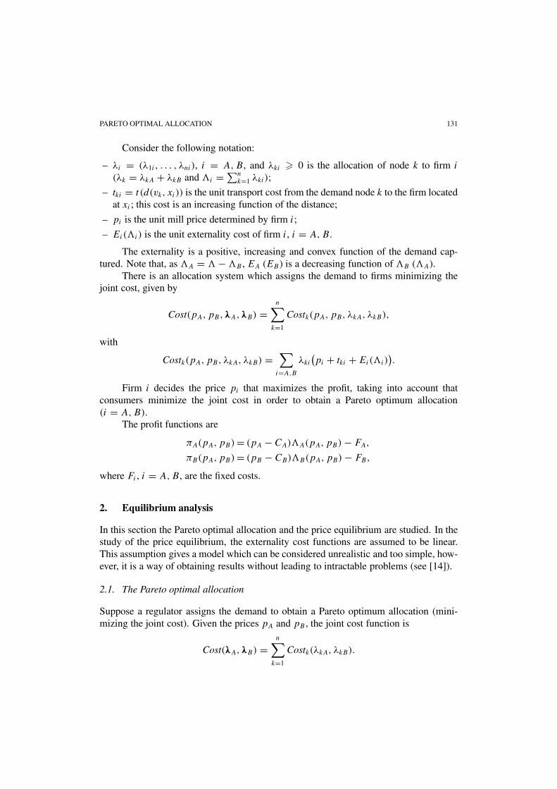
Let
� = {(pA, pB) ∈ �2: pA � CA, pB � CB
},
Rj = � ∩ {(pA, pB) ∈ �2: Lj � pA − pB � Tj−1}, j = 1, . . . , n,
Sj = � ∩ {(pA, pB) ∈ �2: Tj � pA − pB � Lj
}, j = 1, . . . , n − 1,
S0 = � ∩ {(pA, pB) ∈ �2: pA − pB � T0},
Sn = � ∩ {(pA, pB) ∈ �2: pA − pB � Ln
}.
136 DORTA-GONZÁLEZ ET AL.
Figure 2. Equilibrium market shares.
The set
� = [CA,+∞) × [CB,+∞) =(
n⋃j=1
Rj
)∪(
n⋃j=0
Sj
)
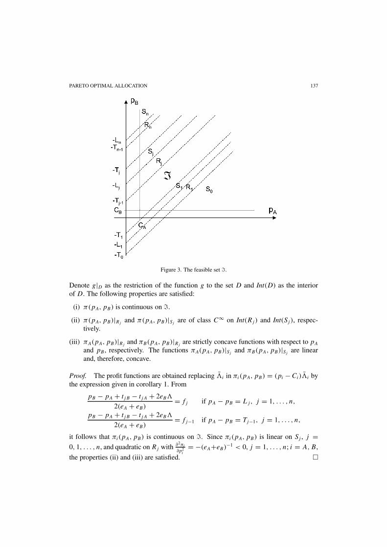
is represented in figure 3.Given two locations, the profit function can be expressed as
πi(pA, pB) = (pi − Ci)�̄i − Fi, i = A,B.
To simplify the notation, null fixed costs (Fi = 0) are assumed. For this case, the profitfunctions are given in the following proposition.
Proposition 4. The profit function π(pA, pB) = (πA(pA, pB), πB(pA, pB)) is definedon � by the expression
((pA − CA)�, 0
)if (pA, pB) ∈ Sn,(
(pA − CA)
(pB − pA + tjB − tjA + 2eB�
2(eA + eB)
),
(pB − CB)
(pA − pB + tjA − tjB + 2eA�
2(eA + eB)
))if (pA, pB) ∈ Rj − (Sj ∪ Sj−1), j = 1, . . . , n,(
(pA − CA)fj, (pB − CB)(� − fj ))
if (pA, pB) ∈ Sj , j = 1, . . . , n − 1,(0, (pB − CB)�
)if (pA, pB) ∈ S0.
PARETO OPTIMAL ALLOCATION 137
Figure 3. The feasible set �.
Denote g|D as the restriction of the function g to the set D and Int(D) as the interiorof D. The following properties are satisfied:
(i) π(pA, pB) is continuous on �.
(ii) π(pA, pB)|Rjand π(pA, pB)|Sj
are of class C∞ on Int(Rj ) and Int(Sj ), respec-tively.
(iii) πA(pA, pB)|Rjand πB(pA, pB)|Rj
are strictly concave functions with respect to pA
and pB , respectively. The functions πA(pA, pB)|Sjand πB(pA, pB)|Sj
are linearand, therefore, concave.
Proof. The profit functions are obtained replacing �̄i in πi(pA, pB) = (pi − Ci)�̄i bythe expression given in corollary 1. From
pB − pA + tjB − tjA + 2eB�
2(eA + eB)= fj if pA − pB = Lj, j = 1, . . . , n,
pB − pA + tjB − tjA + 2eB�
2(eA + eB)= fj−1 if pA − pB = Tj−1, j = 1, . . . , n,
it follows that πi(pA, pB) is continuous on �. Since πi(pA, pB) is linear on Sj , j =0, 1, . . . , n, and quadratic on Rj with ∂2πi
∂p2i
= −(eA+eB)−1 < 0, j = 1, . . . , n; i = A,B,
the properties (ii) and (iii) are satisfied. �
138 DORTA-GONZÁLEZ ET AL.
In order to obtain the price equilibrium, the best-reply functions are calculated inproposition 5.
Proposition 5. The best-reply functions are
rA|S0(pB) = {p: p − pB � T0},rA|Sj
(pB) =pB + Lj, j = 1, . . . , n,
rA|Rj(pB) =
CA if pB � −2Tj−1 + CA + tjB − tjA + 2eB�,r̃j
A(pB) if −2Tj−1 + CA + tjB − tjA + 2eB� < pB
< −2Lj + CA + tjB − tjA + 2eB�,pB + Lj if pB � −2Lj + CA + tjB − tjA + 2eB�,
where r̃j
A(pB) = 12 (pB + CA + tjB − tjA + 2eB�), j = 1, . . . , n,
rB |Sj(pA) =pA − Tj , j = 0, . . . , n − 1,
rB |Sn(pA) = {p: pA − p � Ln},
rB |Rj(pA) =
CB if pA � 2Lj + CB − tjB + tjA + 2eA�,r̃j
B(pA) if 2Lj + CB − tjB + tjA + 2eA� < pA
< 2Tj−1 + CB − tjB + tjA + 2eA�,pA − Tj−1 if pA � 2Tj−1 + CB − tjB + tjA + 2eA�,
where r̃j
B(pA) = 12 (pA + CB − tjB + tjA + 2eA�), j = 1, . . . , n.
Proof. See appendix A. �
If a price equilibrium in � exists, then this equilibrium belongs to one of the regionsSj or Rj . Henceforth as a first approach the partial equilibria in �, that is, the equilibriarestricted to S0, Sj , and Rj , j = 1, 2, . . . , n, will be studied in proposition 6.
Let
LNj = tjB − tjA + 2(eA + 2eB)� − 6(eA + eB)fj , j = 1, . . . , n,
T Nj−1 = tjB − tjA + 2(eA + 2eB)� − 6(eA + eB)fj−1, j = 1, . . . , n.
Then, it can be proved that
LNj = 3Lj − 2(tjB − tjA) + 2(eA − eB)�,
T Nj−1 = 3Tj−1 − 2(tjB − tjA) + 2(eA − eB)�,
LNn < T N
n−1 < LNn−1 < · · · < T N
j < LNj < T N
j−1 < LNj−1 < · · · < T N
1 < LN1 < T N
0 .
Proposition 6 (Partial equilibria in �).
(i) The set of price equilibria in Sn is {(p̄A, p̄B) ∈ Sn: p̄A − p̄B = Ln}.
PARETO OPTIMAL ALLOCATION 139
(ii) The set of price equilibria in S0 is {(p̄A, p̄B) ∈ S0: p̄A − p̄B = T0}.(iii) Equilibrium does not exist in Sj , j = 1, . . . , n − 1.
(iv) There is equilibrium in Rj , j = 1, . . . , n. Moreover,
(a) If LNj � CA − CB � T N
j−1, then (p̃j
A, p̃j
B) is an equilibrium with
p̃j
A = 1
3
[2CA + CB + tjB − tjA + 2(eA + 2eB)�
],
p̃j
B = 1
3
[CA + 2CB + tjA − tjB + 2(2eA + eB)�
].
(b) If CA − CB < LNj , then the prices of the set � ∩ {(p + Lj, p): p1 � p � p2}
are equilibria, with p1 = −2Lj + tjB − tjA + CA + 2eB�, p2 = Lj + tjA −tjB + CB + 2eA�.
(c) If CA−CB > T Nj−1, then the prices of the set �∩{(p+Tj−1, p): p3 � p � p4}
are equilibria, with p3 = Tj−1 + tjA − tjB +CB + 2eA�, p4 = −2Tj−1 + tjB −tjA + CA + 2eB�.
Proof. See appendix A. �
Corollary 2. If LNj < CA − CB < T N
j−1, then (p̃j
A, p̃j
B) is a local equilibrium in �.
Proof. If LNj < CA − CB < T N
j−1, then there exists a ball in Rj ⊂ � where (p̃j
A, p̃j
B) is
an equilibrium, therefore (p̃j
A, p̃j
B) is a local equilibrium in �. �
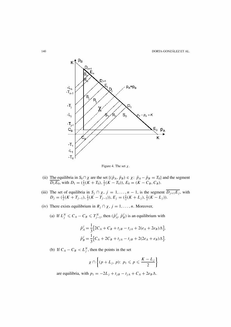
In propositions 7 and 8, partial and global equilibria in the set χ below, are studied.The results are used to prove the existence of a global equilibrium in a rectangular subsetof �.
Let
χ = {(pA, pB) ∈ �2: pA � CA, pB � CB, pA + pB � K
},
with K = CA + CB + 2�(eA + eB). The set χ is represented in figure 4. The restrictionpA + pB � K is used to define the set χ and considers the study of the equilibriumproblem in a compact set. The introduction of this restriction is motivated by the equalityp̃
j
A + p̃j
B = K. Without this restriction, a indefinite increase in prices is possible andthere is not equilibrium in Sj , j = 1, . . . , n−1. On the other hand, an indefinite increasein prices is not realistic and, especially for essential goods, some rules imposing a limitare established.
Proposition 7 (Partial equilibria in χ).
(i) The equilibria in Sn∩χ are the set {(p̄A, p̄B) ∈ χ : p̄A − p̄B = Ln} and the segmentDn+1En, with Dn+1 = (CA,K − CA), En = ( 1
2 (K + Ln),12(K − Ln)).
140 DORTA-GONZÁLEZ ET AL.
Figure 4. The set χ .
(ii) The equilibria in S0 ∩χ are the set {(p̄A, p̄B) ∈ χ : p̄A − p̄B = T0} and the segmentD1E0, with D1 = ( 1
2 (K + T0),12 (K − T0)), E0 = (K − CB,CB).
(iii) The set of equilibria in Sj ∩ χ , j = 1, . . . , n − 1, is the segment Dj+1Ej , withDj = ( 1
2 (K + Tj−1),12(K − Tj−1)), Ej = ( 1
2(K + Lj),12 (K − Lj)).
(iv) There exists equilibrium in Rj ∩ χ , j = 1, . . . , n. Moreover,
(a) If LNj � CA − CB � T N
j−1, then (p̃j
A, p̃j
B) is an equilibrium with
p̃j
A = 1
3
[2CA + CB + tjB − tjA + 2(eA + 2eB)�
],
p̃j
B = 1
3
[CA + 2CB + tjA − tjB + 2(2eA + eB)�
].
(b) If CA − CB < LNj , then the points in the set
χ ∩{(p + Lj, p): p1 � p � K − Lj
2
}
are equilibria, with p1 = −2Lj + tjB − tjA + CA + 2eB�.
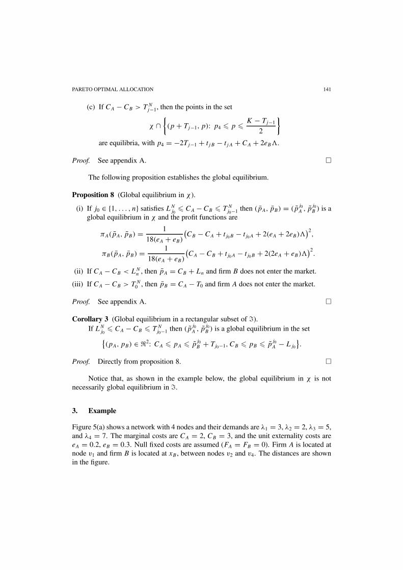
PARETO OPTIMAL ALLOCATION 141
(c) If CA − CB > T Nj−1, then the points in the set
χ ∩{(p + Tj−1, p): p4 � p � K − Tj−1
2
}are equilibria, with p4 = −2Tj−1 + tjB − tjA + CA + 2eB�.
Proof. See appendix A. �
The following proposition establishes the global equilibrium.
Proposition 8 (Global equilibrium in χ).
(i) If j0 ∈ {1, . . . , n} satisfies LNj0
� CA − CB � T Nj0−1 then (p̄A, p̄B) = (p̃
j0A , p̃
j0B ) is a
global equilibrium in χ and the profit functions are
πA(p̄A, p̄B) = 1
18(eA + eB)
(CB − CA + tj0B − tj0A + 2(eA + 2eB)�
)2,
πB(p̄A, p̄B) = 1
18(eA + eB)
(CA − CB + tj0A − tj0B + 2(2eA + eB)�
)2.
(ii) If CA − CB < LNn , then p̄A = CB + Ln and firm B does not enter the market.
(iii) If CA − CB > T N0 , then p̄B = CA − T0 and firm A does not enter the market.
Proof. See appendix A. �
Corollary 3 (Global equilibrium in a rectangular subset of �).If LN
j0� CA − CB � T N
j0−1 then (p̃j0A , p̃
j0B ) is a global equilibrium in the set{
(pA, pB) ∈ �2: CA � pA � p̃j0B + Tj0−1, CB � pB � p̃
j0A − Lj0
}.
Proof. Directly from proposition 8. �
Notice that, as shown in the example below, the global equilibrium in χ is notnecessarily global equilibrium in �.
3. Example
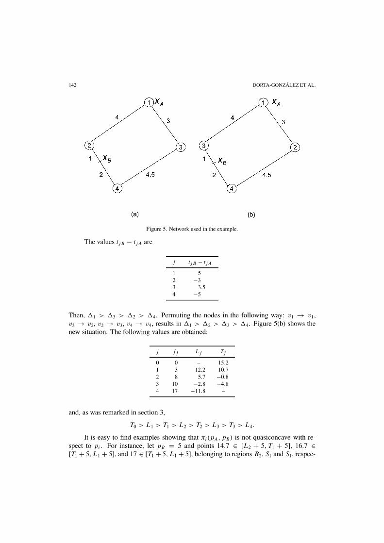
Figure 5(a) shows a network with 4 nodes and their demands are λ1 = 3, λ2 = 2, λ3 = 5,and λ4 = 7. The marginal costs are CA = 2, CB = 3, and the unit externality costs areeA = 0.2, eB = 0.3. Null fixed costs are assumed (FA = FB = 0). Firm A is located atnode v1 and firm B is located at xB , between nodes v2 and v4. The distances are shownin the figure.
142 DORTA-GONZÁLEZ ET AL.
Figure 5. Network used in the example.
The values tjB − tjA are
j tjB − tjA
1 52 −33 3.54 −5
Then, �1 > �3 > �2 > �4. Permuting the nodes in the following way: v1 → v1,v3 → v2, v2 → v3, v4 → v4, results in �1 > �2 > �3 > �4. Figure 5(b) shows thenew situation. The following values are obtained:
j fj Lj Tj
0 0 – 15.21 3 12.2 10.72 8 5.7 −0.83 10 −2.8 −4.84 17 −11.8 –
and, as was remarked in section 3,
T0 > L1 > T1 > L2 > T2 > L3 > T3 > L4.
It is easy to find examples showing that πi(pA, pB) is not quasiconcave with re-spect to pi . For instance, let pB = 5 and points 14.7 ∈ [L2 + 5, T1 + 5], 16.7 ∈[T1 + 5, L1 + 5], and 17 ∈ [T1 + 5, L1 + 5], belonging to regions R2, S1 and S1, respec-
PARETO OPTIMAL ALLOCATION 143
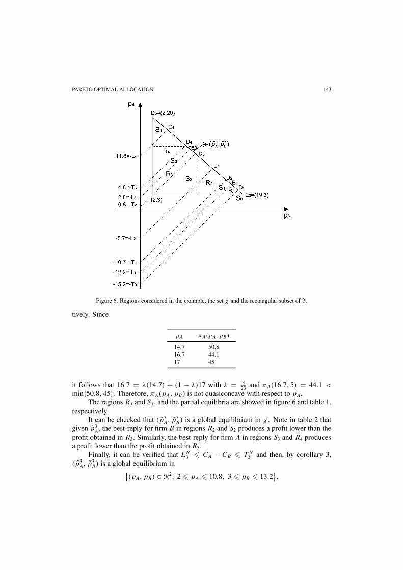
Figure 6. Regions considered in the example, the set χ and the rectangular subset of �.
tively. Since
pA πA(pA, pB)
14.7 50.816.7 44.117 45
it follows that 16.7 = λ(14.7) + (1 − λ)17 with λ = 323 and πA(16.7, 5) = 44.1 <
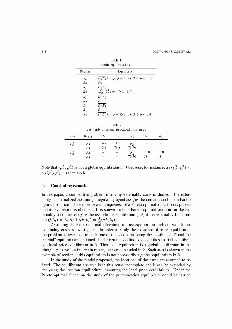
min{50.8, 45}. Therefore, πA(pA, pB) is not quasiconcave with respect to pA.The regions Rj and Sj , and the partial equilibria are showed in figure 6 and table 1,
respectively.It can be checked that (p̃3
A, p̃3B) is a global equilibrium in χ . Note in table 2 that
given p̃3A, the best-reply for firm B in regions R2 and S2 produces a profit lower than the
profit obtained in R3. Similarly, the best-reply for firm A in regions S3 and R4 producesa profit lower than the profit obtained in R3.
Finally, it can be verified that LN3 � CA − CB � T N
2 and then, by corollary 3,(p̃3
A, p̃3B) is a global equilibrium in{
(pA, pB) ∈ �2: 2 � pA � 10.8, 3 � pB � 13.2}.
144 DORTA-GONZÁLEZ ET AL.
Table 1Partial equilibria in χ .
Region Equilibria
S4 D5E4 ∪ {(p, p + 11.8): 2 � p < 5.1}R4 D4S3 D4E3R3 (p̃3
A, p̃3B) = (10.4, 11.6)
S2 D3E2R2 E2S1 D2E1R1 E1S0 D1E0 ∪ {(p + 15.2, p): 3 � p < 3.4}
Table 2Best-reply price and associated profit in χ .
Fixed Reply R2 S2 R3 S3 R4
p̃3A
pB 4.7 11.2 p̃3B
– –πB 15.3 73.8 73.96 – –
p̃3B
pA – – p̃3A
8.8 6.8πA – – 70.56 68 48
Note that (p̃3A, p̃
3B) is not a global equilibrium in � because, for instance, πB(p̃3
A, p̃3B) <
πB(p̃3A, p̃
3A − T3) = 85.4.
4. Concluding remarks
In this paper, a competitive problem involving externality costs is studied. The exter-nality is internalized assuming a regulating agent assigns the demand to obtain a Paretooptimal solution. The existence and uniqueness of a Pareto optimal allocation is provedand its expression is obtained. It is shown that the Pareto optimal solution for the ex-ternality functions Ei(q) is the user-choice equilibrium [1,2] if the externality functionsare Qi(q) = Ei(q) + qE′
i (q) = ddq (qEi(q)).
Assuming the Pareto optimal allocation, a price equilibrium problem with linearexternality costs is investigated. In order to study the existence of price equilibrium,the problem is restricted to each one of the sets partitioning the feasible set � and the“partial” equilibria are obtained. Under certain conditions, one of these partial equilibriais a local price equilibrium in �. This local equilibrium is a global equilibrium in thetriangle χ as well as in certain rectangular area included in �. Such as it is shown in theexample of section 4, this equilibrium is not necessarily a global equilibrium in �.
In the study of the model proposed, the locations of the firms are assumed to befixed. The equilibrium analysis is in this sense incomplete and it can be extended byanalyzing the location equilibrium, assuming the local price equilibrium. Under thePareto optimal allocation the study of the price-location equilibrium could be carried
PARETO OPTIMAL ALLOCATION 145
out as a two-stage game in a similar way to other equilibrium problems analyzed in lit-erature [13,17]. Firstly, the locations are chosen and then, given these, the prices aredetermined. To obtain the equilibrium an inverse process is applied; given the locations,the price equilibrium is inferred and then, using this information, the location equilib-rium is obtained.
Other extensions to the problem result from considering different hypothesis inthe definition of the model, such as price-elastic demand functions, a leader–followerbehaviour in price, an oligopolistic market and more general externality cost functions.
Acknowledgments
We wish to thank two anonymous referees for their helpful comments.
Appendix A
A.1. Proof of proposition 3
The necessary and sufficient Karush–Kuhn–Tucker conditions for the allocation problemare:
d
dq
(TEC(q)
) − �k + µk � 0, k = 1, . . . , n,[d
dq
(TEC(q)
)− �k + µk
]λkA = 0, k = 1, . . . , n,
µk(λk − λkA) = 0, k = 1, . . . , n,
µk � 0, k = 1, . . . , n,
0 � λkA � λk, k = 1, . . . , n.
Then one of the following three cases occurs:(a) q̄ = 0. If q̄ = 0, then λ̄kA = 0, k = 1, . . . , n. From KKT conditions it follows
that µk = 0 and ddq (TEC(q))|0 − �k � 0, k = 1, . . . , n. Therefore,
q̄ = 0 ⇐⇒ λ̄kA = 0, k = 1, . . . , n
⇐⇒ d
dq
(TEC(q)
)∣∣∣∣0
� �k, k = 1, . . . , n.
(b) q̄ = �. Now λ̄kA = λk, k = 1, . . . , n, and by KKT conditions, ddq (TEC(q))|�−
�k + µk = 0, where µk � 0, k = 1, . . . , n. Therefore, ddq (TEC(q))|� − �k � 0,
k = 1, . . . , n. Then
q̄ = � ⇐⇒ λ̄kA = λk, k = 1, . . . , n
⇐⇒ d
dq
(TEC(q)
)∣∣∣∣�
� �k, k = 1, . . . , n.
146 DORTA-GONZÁLEZ ET AL.
(c) 0 < q̄ < �. If 0 < q̄ < �, then there exists 1 � j � n such that fj−1 � q̄ �fj . As a result, one of the following cases occurs:
(c.1) q̄ = fj , j = 1, . . . , n − 1. In this case, λ̄kA = λk if k � j and λ̄kA = 0 ifk > j . Then, by KKT conditions,
d
dq
(TEC(q)
)∣∣∣∣fj
− �k + µk = 0 if k � j,
d
dq
(TEC(q)
)∣∣∣∣fj
− �k � 0 if k > j.
That is,
d
dq
(TEC(q)
)∣∣∣∣fj
� �k if k � j,
d
dq
(TEC(q)
)∣∣∣∣fj
� �k if k > j.
Therefore,
�j+1 � d
dq
(TEC(q)
)∣∣∣∣fj
� �j.
(c.2) fj−1 < q̄ < fj , j = 1, . . . , n. In this case, λ̄kA = λk if k � j − 1,λ̄jA = q̄ − fj−1 and λ̄kA = 0 if k > j . Then, by KKT conditions,
d
dq
(TEC(q)
)∣∣∣∣q̄
− �k + µk = 0 if k � j − 1,
µk = 0 andd
dq
(TEC(q)
)∣∣∣∣q̄
− �k = 0 if k = j,
µk = 0 andd
dq
(TEC(q)
)∣∣∣∣q̄
− �k � 0 if k > j.
That is,
d
dq
(TEC(q)
)∣∣∣∣q̄
��k if k � j − 1,
d
dq
(TEC(q)
)∣∣∣∣q̄
=�k if k = j,
d
dq
(TEC(q)
)∣∣∣∣q̄
��k if k > j.
Therefore,d
dq
(TEC(q)
)∣∣∣∣q̄
= �j.
The value of q̄ is obtained from (a), (b) and (c).
PARETO OPTIMAL ALLOCATION 147
A.2. Proof of proposition 5
The profit πA(pA, pB) is
(pA − CA)� if (pA, pB) ∈ Sn,
(pA − CA)
(pB − pA + tjB − tjA + 2eB�
2(eA + eB)
)if (pA, pB) ∈ Rj − (Sj ∪ Sj−1),
j = 1, . . . , n,(pA − CA)fj if (pA, pB) ∈ Sj , j = 1, . . . , n − 1,0 if (pA, pB) ∈ S0.
Since πA|S0(pA, pB) = 0 and πA|Sj(pA, pB) = (pA − CA)fj , ∀j > 0, then
rA|S0(pB) = {p: p − pB � T0} and rA|Sj(pB) = pB + Lj, ∀j > 0.
Let
ϕ(pA) = (pA − CA)
(pB − pA + tjB − tjA + 2eB�
2(eA + eB)
).
Then
ϕ′(pA) = 0 ⇐⇒ pA = 1
2(pB + CA + tjB − tjA + 2eB�).
Let
p∗A = 1
2(pB + CA + tjB − tjA + 2eB�),
then Lj < p∗A − pB < Tj−1 if and only if
−2Tj−1 + CA + tjB − tjA + 2eB� < pB < −2Lj + CA + tjB − tjA + 2eB�.
Moreover, under the previous condition, p∗A > CA. Since ϕ′′(pA) < 0, the function
ϕ(pA) is concave and
rA|Rj(pB) =
CA = max{pB + Tj−1, CA}if pB � −2Tj−1 + CA + tjB − tjA + 2eB�,
r̃j
A(pB) if − 2Tj−1 + CA + tjB − tjA + 2eB� < pB
< −2Lj + CA + tjB − tjA + 2eB�,
pB + Lj if pB � −2Lj + CA + tjB − tjA + 2eB�.
Note that pB + Lj � CA if pB � −2Lj + CA + tjB − tjA + 2eB�. Moreover,
πB(pA, pB) =
0 if (pA, pB) ∈ Sn,
(pB − CB)
(pA − pB − tjB + tjA + 2eA�
2(eA + eB)
)if (pA, pB) ∈ Rj − (Sj ∪ Sj−1), j = 1, . . . , n,
(pB − CB)(� − fj ) if (pA, pB) ∈ Sj , j = 1, . . . , n − 1,(pB − CB)� if (pA, pB) ∈ S0.
148 DORTA-GONZÁLEZ ET AL.
Since πB |Sn(pA, pB) = 0 and πB |Sj
(pA, pB) = (pB − CB)(� − fj ), ∀j < n, then
rB |Sn(pA) = {p: pA − p � Ln} and rB |Sj
(pA) = pA − Tj , ∀j < n.
Let
ψ(pB) = (pB − CB)
(pA − pB − tjB + tjA + 2eA�
2(eA + eB)
).
Then,
ψ ′(pB) = 0 ⇐⇒ pB = 1
2(pA + CB − tjB + tjA + 2eA�).
Let
p∗B = 1
2(pA + CB − tjB + tjA + 2eA�),
then Lj < pA − p∗B < Tj−1 if and only if
2Lj + CB − tjB + tjA + 2eA� < pA < 2Tj−1 + CB − tjB + tjA + 2eA�.
Moreover, under the previous condition, p∗B > CB . Since ψ ′′(pB) < 0, the function
ψ(pB) is concave and
rB |Rj(pA) =
CB = max{pA − Lj,CB} if pA � 2Lj + CB − tjB + tjA + 2eA�,r̃j
B(pA) if 2Lj + CB − tjB + tjA + 2eA� < pA
< 2Tj−1 + CB − tjB + tjA + 2eA�,pA − Tj−1 if pA � 2Tj−1 + CB − tjB + tjA + 2eA�.
A.3. Proof of proposition 6
(i) Let (p̄A, p̄B) ∈ Sn such that p̄A − p̄B = Ln. Then
rA|Sn(p̄B) = p̄A,
p̄B ∈ rB |Sn(p̄A),
therefore (p̄A, p̄B) is an equilibrium in Sn. Moreover, if p̄A − p̄B < Ln then (p̄A, p̄B) isnot an equilibrium in Sn. That is, if p̄A − p̄B + h = Ln, with h > 0, then rA|Sn
(p̄B) =p̄A + h and (p̄A, p̄B) is not an equilibrium in Sn.
(ii) Let (p̄A, p̄B) ∈ S0 such that p̄A − p̄B = T0. Then
p̄A ∈ rA|S0(p̄B),
rB |S0(p̄A) = p̄B,
therefore (p̄A, p̄B) is an equilibrium in S0. Moreover, if p̄A − p̄B > T0 then (p̄A, p̄B) isnot an equilibrium in S0.
(iii) The profits πi(pA, pB), i = A,B, are linear and nondecreasing functionson Sj , j = 0, . . . , n. For each point (pA, pB) ∈ Sj there exists (p′
A, p′B) ∈ Sj such that
p′A > pA or p′
B > pB . Therefore
πA(p′A, pB) > πA(pA, pB) or πB(pA, p
′B) > πB(pA, pB),
PARETO OPTIMAL ALLOCATION 149
and (pA, pB) is not an equilibrium point.
(iv) Let j ∈ {1, . . . , n}.(a) If LN
j � CA − CB � T Nj−1 then (p̃
j
A, p̃j
B) ∈ Rj and is a fixed point of r|Rj=
(rA|Rj, rB |Rj
).(b) If CA − CB < LN
j then the equilibrium is located in the frontier of Rj , in theline pA − pB = Lj . Let (p̄A, p̄B) = (p + Lj, p), that is, (p̄A, p̄B) is a point on the linepA − pB = Lj . Then,
r̃j
A(p) = 1
2(p + CA + tjB − tjA + 2eB�) � p + Lj
⇐⇒ p � −2Lj + tjB − tjA + CA + 2eB� = p1,
r̃j
B(p + Lj) = 1
2(p + Lj + CB + tjA − tjB + 2eA�) � p
⇐⇒ p � Lj + tjA − tjB + CB + 2eA� = p2.
Since CA − CB < LNj , it is easy to check that p1 < p2. Then, any point (p + Lj, p),
p1 � p � p2, in � is an equilibrium. Note that Ej , represented in figure 4, is themid-point between (p1 + Lj, p1) and (p2 + Lj, p2).
(c) If CA − CB > T Nj−1 then the equilibrium is located on the frontier of Rj , in the
line pA − pB = Tj−1. Let (p̄A, p̄B) = (p + Tj−1, p), that is, (p̄A, p̄B) is a point on theline pA − pB = Tj−1. Then,
rA|Rj(p) = 1
2(p + CA + tjB − tjA + 2eB�) � p + Tj−1
⇐⇒ p � −2Tj−1 + tjB − tjA + CA + 2eB� = p4,
rB |Rj(p + Tj−1) = 1
2(p + Tj−1 + CB + tjA − tjB + 2eA�) � p
⇐⇒ p � Tj−1 + tjA − tjB + CB + 2eA� = p3.
Since CA − CB > T Nj−1, it is easy to check that p3 < p4. Then, any point (p + Tj−1, p),
p3 � p � p4, in � is an equilibrium. Note that Dj , represented in figure 4, is themid-point between (p3 + Tj−1, p3) and (p4 + Tj−1, p4).
A.4. Proof of proposition 7
(i) The points (p̄A, p̄B) ∈ χ such that p̄A − p̄B = Ln are equilibria in Sn and, therefore,are equilibria in Sn ∩ χ ⊂ Sn. On the other hand, πB(pA, pB) = 0 and πA(pA, pB) islinear and increasing in Sn. If (pA, pB) ∈ Dn+1En, then rA(pB) = pA and pB ∈ rB(pA),therefore (pA, pB) is an equilibrium.
Any other point in Sn ∩ χ is not an equilibrium (similar to proposition 6(i)).(ii) The points (p̄A, p̄B) ∈ χ such that p̄A − p̄B = L0 are equilibria in S0 and,
therefore, are equilibria in S0 ∩ χ ⊂ S0. On the other hand, πA(pA, pB) = 0 andπB(pA, pB) is linear and increasing in S0. If (pA, pB) ∈ D1E0, then pA ∈ rA(pB) andrB(pA) = pB , therefore (pA, pB) is an equilibrium.
150 DORTA-GONZÁLEZ ET AL.
Any other point in S0 ∩ χ is not an equilibrium (similar to proposition 6(ii)).(iii) The profit functions πi(pA, pB), i = A,B, are linear and increasing in
Sj ∩ χ , j = 1, . . . , n − 1. Given (pA, pB) ∈ Dj+1Ej , then rA(pB) = pA andrB(pA) = pB , therefore (pA, pB) is an equilibrium. On the other hand, given (pA, pB) ∈{(Sj ∩ χ) − Dj+1Ej } there exists (p′
A, p′B) ∈ Sj ∩ χ such that p′
A > pA or p′B > pB ,
therefore πA(p′A, pB) > πA(pA, pB) or πB(pA, p
′B) > πB(pA, pB), and (pA, pB) is not
an equilibrium.(iv) (a) If LN
j � CA − CB � T Nj−1 then (p̃
j
A, p̃j
B) is an equilibrium in Rj (propo-
sition 6(iv)). Moreover, p̃j
A + p̃j
B = K and then (p̃j
A, p̃j
B) ∈ Rj ∩ χ ⊂ Rj . Therefore,(p̃
j
A, p̃j
B) is an equilibrium in Rj ∩ χ .(b) If CA − CB < LN
j then the points χ ∩ {(p + Lj, p): p1 � p � (K − Lj)/2}are equilibria in Rj (proposition 6(iv)). Therefore, these points are equilibria in Rj ∩ χ .
(c) Similar to (b).
A.5. Proof of proposition 8
(i) It will be proved, that given p̃j0B , the best-reply for firm A is p̃
j0A and vice versa. If
LNj0
� CA − CB � T Nj0−1 then (p̃
j0A , p̃
j0B ) ∈ Rj0 and{
(pA, p̃j0B ): pA � CA
} ∩ (Sj ∩ χ) = ∅, ∀j < j0,{(pA, p̃
j0B ): pA � CA
} ∩ (Rj ∩ χ) = ∅, ∀j < j0,{(p̃
j0A , pB): pB � CB
} ∩ (Sj ∩ χ) = ∅, ∀j � j0,{(p̃
j0A , pB): pB � CB
} ∩ (Rj ∩ χ) = ∅, ∀j > j0.
(i.1) Let pB = p̃j0B and j � j0 + 1 such that
(Rj ∩ χ) ∩ {(pA, p̃j0B
): pA � CA
} �= ∅.Since tj0B − tj0A > tjB − tjA, ∀j � j0 + 1, then
πA|Rj0
(pA, p̃
j0B
)= (pA − CA)
(p̃
j0B − pA + tj0B − tj0A + 2eB�
2(eA + eB)
)
> (pA − CA)
(p̃
j0B − pA + tjB − tjA + 2eB�
2(eA + eB)
)=πA|
Rj
(pA, p̃
j0B
), ∀pA � CA.
Therefore,
max(pA,p̃
j0B )∈Rj0
πA|Rj0
(pA, p̃
j0B
)= maxpA�CA
πA|Rj0
(pA, p̃
j0B
)� max
(pA,p̃j0B )∈Rj
πA|Rj
(pA, p̃
j0B
).
PARETO OPTIMAL ALLOCATION 151
(i.2) Let pB = p̃j0B and j � j0 such that
(Sj ∩ χ) ∩ {(pA, p̃j0B
): pA � CA
} �= ∅.Then, taking into account (i.1) it follows that
πA
(p̃
j0A , p̃
j0B
)� max
(pA,p̃j0B )∈Rj
πA|Rj
(pA, p̃
j0B
)� max
(pA,p̃j0B )∈Rj∩Sj
πA|Rj
(pA, p̃
j0B
)= max
(pA,p̃j0B )∈Sj
πA|Sj
(pA, p̃
j0B
) = πA
(Lj + p̃
j0B , p̃
j0B
).
(i.3) In a similar way to (i.1), let pA = p̃j0A and j � j0 − 1 such that (Rj ∩ χ) ∩
{(p̃j0A , pB): pB � CB} �= ∅. Since tj0A − tj0B > tjA − tjB , ∀j � j0 − 1, it follows that
πB |Rj0
(p̃
j0A , pB
)= (pB − CB)
(p̃
j0A − pB + tj0A − tj0B + 2eA�
2(eA + eB)
)
> (pB − CB)
(p̃
j0A − pB + tjA − tjB + 2eA�
2(eA + eB)
)=πB |
Rj
(p̃
j0A , pB
), ∀pB � CB.
Therefore
max(p̃
j0A ,pB)∈Rj0
πB |Rj0
(p̃
j0A , pB
)= maxpB�CB
πB |Rj0
(p̃
j0A , pB
)� max
(p̃j0A ,pB)∈Rj
πB |Rj
(p̃
j0A , pB
).
(i.4) In a similar way to (i.2), let pA = p̃j0A and j � j0 − 1 such that (Sj ∩ χ) ∩
{(p̃j0A , pB): pB � CB} �= ∅. Then,
πB
(p̃
j0A , p̃
j0B
)� max
(p̃j0A ,pB)∈Rj+1
πB |Rj+1
(p̃
j0A , pB
)� max
(p̃j0A ,pB)∈Rj+1∩Sj
πB |Rj+1
(p̃
j0A , pB
)= max
(p̃j0A ,pB)∈Sj
πB |Sj
(p̃
j0A , pB) = πB
(p̃
j0A , p̃
j0A − Tj
).
(ii) If CA − CB < LNn , then p̄A − pB � p̄A − CB = Ln, ∀pB � CB , therefore
(p̄A, pB) ∈ Sn. In this case, A captures all the demand and the best-reply for B is not toenter the market.
On the other hand, if B does not enter the market, the demand will be satisfied by A.The best-reply for A will be the maximum price in the region Sn, that is p̄A = CB + Ln.
(iii) Proceeding in a similar way to (ii).
152 DORTA-GONZÁLEZ ET AL.
References
[1] M. Brandeau and S.S. Chiu, Facility location in a user-optimizing environment with market external-ities: Analysis of customer equilibria and optimal public facility locations, Location Science 2 (1994)129–147.
[2] M. Brandeau and S.S. Chiu, Location of competing private facilities in a user-optimizing environmentwith market externalities, Transportation Science 28 (1994) 125–140.
[3] R. Corner and T. Sandler, The Theory of Externalities, Public Goods, and Club Goods (CambridgeUniversity Press, New York, 1986).
[4] P. Dorta-González, Problemas de equilibrio en modelos de competencia espacial en redes, Ph.D.thesis, University of Las Palmas de Gran Canaria, Spain (2001).
[5] H.A. Eiselt and G. Laporte, Competitive spatial models, European Journal of Operation Research 39(1989) 231–242.
[6] H.A. Eiselt and G. Laporte, Equilibrium results in competitive location models, Middle East Forum 1(1996) 63–92.
[7] H.A. Eiselt, G. Laporte and J.-F. Thisse, Competitive location models: A framework and bibliography,Transportation Science 27 (1993) 44–54.
[8] J.W. Friedman, Game Theory with Applications to Economics (Oxford University Press, New York,1991).
[9] T.L. Friesz, T. Miller and R.L. Tobin, Competitive network facility location models: A survey, Papersof the Regional Science Association 65 (1988) 47–57.
[10] S.L. Hakimi, On locating new facilities in a competitive environment, European Journal of Opera-tional Research 12 (1983) 29–35.
[11] H. Hotelling, Stability in competition, Economic Journal 39 (1929) 41–57.[12] E. Kohlberg, Equilibrium store locations when consumers minimize travelling time plus waiting time,
Economics Letters 11 (1983) 211–216.[13] M. Labbé and S.L. Hakimi, Market and location equilibrium for two competitors, Operation Research
39 (1991) 749–756.[14] M. Laurent, D. Peeters and I. Thomas, Spatial externalities and optimal locations. Simulations on a
theoretical network, Studies in Locational Analysis 11 (1997) 193–210.[15] P.J. Lederer and J.-F. Thisse, Competitive location on networks under delivered pricing, Operational
Research Letters 9 (1990) 147–153.[16] J.B. Rosen, Existence and uniqueness of equilibrium points for concave n-person games, Economet-
rica 33 (1965) 520–534.[17] J. Sarkar, B. Gupta and D. Pal, Location equilibrium for Cournot oligopoly in spatially separated
markets, Journal of Regional Science 2 (1997) 195–212.[18] R. Selten, Reexamination of the perfectness concept for equilibrium points in extensive games, Inter-
national Journal of Game Theory 4 (1975) 25–55.[19] R. Suárez-Vega, P. Dorta-González and D.-R. Santos-Peñate, Externality in a Stackelberg spatial com-
petition model, Studies in Locational Analysis 14 (2000) 205–223.[20] J. Tirole, The Theory of Industrial Organization (MIT Press, Cambridge, MA, 1988).[21] R.L. Tobin and T.L. Friesz, Spatial competition facility location models: definition, formulation and
solution approach, Annals of Operation Research 6 (1986) 49–74.