Commun. Comput. Phys.doi: 10.4208/cicp.210910.200611a

Vol. 12, No. 1, pp. 65-84July 2012

A Coupled Approach for Fluid Dynamic Problems

Using the PDE Framework Peano

Philipp Neumann∗, Hans-Joachim Bungartz, Miriam Mehl,Tobias Neckel and Tobias Weinzierl

Chair of Scientific Computing, Faculty of Informatics, Technische Universitat Munchen,Boltzmannstr. 3, 81545 Garching, Germany.

Received 21 September 2010; Accepted (in revised version) 20 June 2011

Available online 19 January 2012

Abstract. We couple different flow models, i.e. a finite element solver for the Navier-Stokes equations and a Lattice Boltzmann automaton, using the framework Peano as acommon base. The new coupling strategy between the meso- and macroscopic solveris presented and validated in a 2D channel flow scenario. The results are in goodagreement with theory and results obtained in similar works by Latt et al. In addition,the test scenarios show an improved stability of the coupled method compared to pureLattice Boltzmann simulations.

AMS subject classifications: 35Q30, 35Q35, 76M10, 76-xx

Key words: Spatial coupling, Lattice Boltzmann, Navier-Stokes, Peano.

1 Introduction

Many flow systems – especially in micro- and nano-fluidics – are strongly influenced byphysical processes that appear on different spatial and temporal scales. Flows throughnanopores influenced by Brownian motion or flows in porous media are typical exam-ples. Solving these kinds of complex systems by means of computational fluid dynamics(CFD) often requires highly adaptive concepts or different sorts of solvers depending onthe current scale to be simulated.

With respect to Navier-Stokes and Lattice Boltzmann related solver techniques, de-tailed discussions and comparisons of their performance and qualitative behaviour canamongst others be found in [8, 13] and should only be touched here. Considering flowproblems on mesoscopic scales, Lattice Boltzmann methods have been validated for awide range of scenarios such as particulate flows [10] or fluctuating hydrodynamics

∗Corresponding author. Email address: neumanph@in.tum.de (P. Neumann)

http://www.global-sci.com/ 65 c©2012 Global-Science Press

66 P. Neumann et al. / Commun. Comput. Phys., 12 (2012), pp. 65-84

[7]. Furthermore, as discussed in our previous works [13], simulation tests by differ-ent groups in the finite Knudsen number regime revealed strong deviations of macro-scopic Navier-Stokes and Burnett descriptions from the physical phenomena (cf. [17,18])whereas mesoscopic approaches like Direct Simulation Monte Carlo and Lattice Boltz-mann methods still yielded feasible results [9, 21]. On the other hand, Navier-Stokessystems might e.g. be superior in case of (laminar) convection dominated flows whereclassical Lattice Boltzmann automata often require even finer grid resolutions and smalltimesteps. Implicit solver strategies for the Navier-Stokes equations would allow for con-siderably bigger timesteps in these cases.

With implementations of a Navier-Stokes and a Lattice Boltzmann solver integratedwithin the Peano framework, we already deeply discussed and evaluated the singlecodes in [13]; it is in this context that the idea emerged to spatially couple both approachesand exploit the advantages of both schemes as also proposed by Latt et al. in [12]. Thereare different scenarios, where this idea might become favorable. Amongst others, consi-dering fluid-structure interaction problems in the laminar flow regime, the weakly com-pressible Lattice Boltzmann method could be used to stabilize pressure induced pertur-bations in the surrounding of the respective structure, whereas the Navier-Stokes equa-tions are solved further away from the structure. Besides, in the case of simulations ofmultiscale flow problems, like laminar flows near and through porous structures suchas membranes, a spatial coupling of Navier-Stokes and Lattice Boltzmann solvers mightallow to resolve the complex geometry of the porous medium and describe this part ofthe flow system by means of Lattice Boltzmann and – on a coarser grid – to compute therest of the flow domain efficiently by (implicit) Navier-Stokes solver techniques.

There have already been several works on this field (see for example [1,12]). It is parti-cularly the work presented in [12] where the coupling between a finite difference Navier-Stokes solver and a Lattice Boltzmann automaton is established and validated. Thoughparts of the respective algorithmic realisations carry over to our coupling approach, wewant to focus on a new method for the macro-to-mesoscale coupling which is based ona minimisation procedure. We particularly point out the feasibility of coupling differenttypes of solvers within the Peano framework.

This paper is structured as follows: The theoretical foundation for the Lattice Boltz-mann method and our Navier-Stokes solver is briefly reviewed in Section 2. Besides, theChapman-Enskog expansion connecting the meso- and macroscopic approach is carriedout in order to obtain the conservation laws that need to be fulfilled at the interface be-tween the two solvers. In Section 3, we give a short introduction to the framework Peanoand discuss its basic properties at the example of our Lattice Boltzmann implementation.In Section 4, we discuss the underlying grid topology and afterwards focus on the metho-dology for coupling Navier-Stokes to Lattice Boltzmann and vice versa. A description ofthe underlying implementations within the Peano framework is given in Section 5. Re-sults for the coupling applied to pure channel flow are provided in Section 6. Finally, weclose the discussion and give a short conclusion and outlook on future work in Section 7.

P. Neumann et al. / Commun. Comput. Phys., 12 (2012), pp. 65-84 67

2 Macro- and mesoscopic simulation methods

2.1 Navier-Stokes equations

The common macroscopic description of flow problems is given by the Navier-Stokesequations describing the conservation of mass and momentum for an incompressiblefluid:

∇·u=0, (2.1)

∂tu+(u·∇)u=−∇p+ν∆u, (2.2)

where u∈RD denotes the flow velocity, p∈R is the pressure and ν defines the kinematic

viscosity. A finite element approach to solve this system of partial differential equationsis implemented in Peano [14]. It uses d-linear elements in space and supports differenttimestepping schemes such as explicit/ implicit Euler or Crank-Nicholson. However, asLattice Boltzmann is a pure explicit scheme, only the explicit Euler timestepping is to beused. The solving of the Navier-Stokes system is accomplished by a Chorin projectionleading to a Poisson equation for the pressure that needs to be solved in every timestepdt, such that each timestep involves three steps:

• Compute the right hand side of the pressure Poisson equation from velocity valuesat time t.

• Solve the Poisson equation to obtain pressure values p(t+dt).

• Update the velocity field using the old velocity values u(t) and the new pressurevalues p(t+dt).

The boundary conditions for the system (Dirichlet or Neumann conditions) can be setdirectly via the velocity values and the assembling method for the right hand side of thePoisson equation; see [14] for more details.

2.2 Lattice Boltzmann method

A mesoscopic approach to computational fluid dynamics is derived from the Boltzmannequation and is known as the Lattice Boltzmann method. Detailed descriptions of themethod can amongst others be found in [16, 20]; a short introduction to its principles isprovided in the following.

Space is discretised with cubic cells, and the velocity space is broken down to a min-imal isotropic set of discrete velocities ci ∈R

D, i∈{1,··· ,Q}, allowing fluid molecules toeither move to a neighbouring cell or to rest in the current one. The update rule to deter-mine the probability fi(x,t) to find fluid molecules at position x∈R

D at time t movingwith velocity ci reads

fi(x+cidt,t+dt)= fi(x,t)+∆i( f − f eq), (2.3)

68 P. Neumann et al. / Commun. Comput. Phys., 12 (2012), pp. 65-84

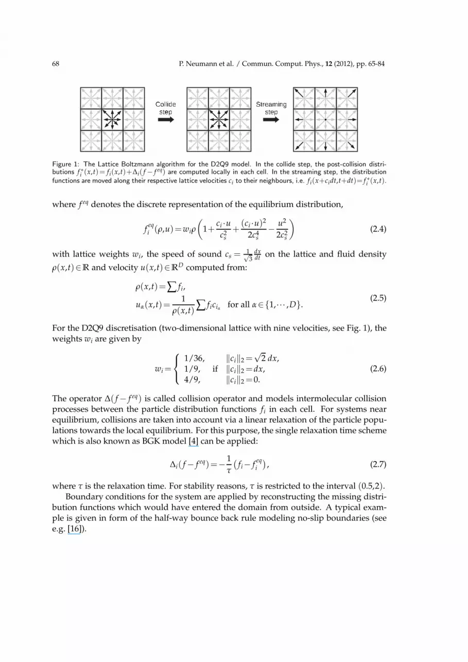
Figure 1: The Lattice Boltzmann algorithm for the D2Q9 model. In the collide step, the post-collision distri-butions f ∗i (x,t)= fi(x,t)+∆i( f − f eq) are computed locally in each cell. In the streaming step, the distributionfunctions are moved along their respective lattice velocities ci to their neighbours, i.e. fi(x+cidt,t+dt)= f ∗i (x,t).

where f eq denotes the discrete representation of the equilibrium distribution,

feqi (ρ,u)=wiρ

(

1+ci ·uc2

s

+(ci ·u)2

2c4s

− u2

2c2s

)

(2.4)

with lattice weights wi, the speed of sound cs =1√3

dxdt on the lattice and fluid density

ρ(x,t)∈R and velocity u(x,t)∈RD computed from:

ρ(x,t)=∑ fi,

uα(x,t)=1

ρ(x,t)∑ ficiαfor all α∈{1,··· ,D}.

(2.5)

For the D2Q9 discretisation (two-dimensional lattice with nine velocities, see Fig. 1), theweights wi are given by

wi=

1/36, ‖ci‖2 =√

2 dx,1/9, if ‖ci‖2 =dx,4/9, ‖ci‖2 =0.

(2.6)

The operator ∆( f − f eq) is called collision operator and models intermolecular collisionprocesses between the particle distribution functions fi in each cell. For systems nearequilibrium, collisions are taken into account via a linear relaxation of the particle popu-lations towards the local equilibrium. For this purpose, the single relaxation time schemewhich is also known as BGK model [4] can be applied:

∆i( f − f eq)=− 1

τ

(

fi− feqi

)

, (2.7)

where τ is the relaxation time. For stability reasons, τ is restricted to the interval (0.5,2).Boundary conditions for the system are applied by reconstructing the missing distri-

bution functions which would have entered the domain from outside. A typical exam-ple is given in form of the half-way bounce back rule modeling no-slip boundaries (seee.g. [16]).

P. Neumann et al. / Commun. Comput. Phys., 12 (2012), pp. 65-84 69

2.3 Chapman-Enskog theory

In order to connect the meso- and macroscales, the Chapman-Enskog expansion [6] canbe used to recover the Navier-Stokes equations from the Lattice Boltzmann equation inthe continuum limit, that is in case that the Knudsen number

ǫ :=L

LH(2.8)

vanishes. In Eq. (2.8), L and LH denote the length scales of the mesoscopic and the hydro-dynamic (macroscopic) system. As the coupling of Navier-Stokes and Lattice Boltzmannsystems strongly depends on the relation between macro- and mesoscopic quantities, thebasic steps of the asymptotic analysis are carried out in the following.

The spatial coordinate xH of the macroscopic description in hydrodynamics can berelated linearly to its mesoscopic representation x which is used in the Lattice Boltzmannscheme:

xH :=ǫx. (2.9)

In order to capture both convective and diffusive phenomena appearing on different tem-poral scales, the hydrodynamic times tC and tD are introduced and can be related to theLattice Boltzmann time t as follows:

tC :=ǫt,

tD :=ǫ2t.(2.10)

In a first step, the left hand side of Eq. (2.3) is expanded in a Taylor series around (x,t):

fi(x+cidt,t+dt)= fi(x,t)+∑α

ciαdt∂xα fi(x,t)+dt∂t fi(x,t)+

dt2

2 ∑α,β

ciαciβ

∂xα ∂xβfi(x,t)

+dt2∑α

∂xα ∂t fi(x,t)+dt2

2∂2

t fi(x,t)+O(dt3). (2.11)

In addition, the distribution functions fi are expanded in an asymptotic series near equi-librium:

fi = feqi +ǫ f

(1)i +O(ǫ2) (2.12)

with the non-equilibrium part fneqi = ǫ f

(1)i . As the density and momentum do not differ

between the equilibrium and non-equilibrium state (see Eq. (2.5)), the non-equilibriumcontributions vanish:

∑i

fneqi =0, (2.13)

∑i

fneqi ciα

=0 for all α∈{1,··· ,D}. (2.14)

70 P. Neumann et al. / Commun. Comput. Phys., 12 (2012), pp. 65-84

The right hand side of Eq. (2.3) is expanded analogously to Eq. (2.12):

fi+∆i( f − f eq)

= feqi +∆

(0)i ( f − f eq)+ǫ

(

f(1)i +∆

(1)i ( f − f eq)

)

+ǫ2∆(2)i ( f − f eq)+O(ǫ3). (2.15)

Introducing the macroscopic scaling for space and time from Eqs. (2.9) and (2.10) inEq. (2.11), i.e.

fi(x,t)= fi(xH(x),tC(t),tD(t)),

∂t =ǫ∂tC+ǫ2∂tD

,

∂xα =ǫ∂xHαfor all α∈{1,··· ,D}, (2.16)

one obtains:

fi(x+cidt,t+dt)= feqi +ǫ

(

f(1)i +∑

α

ciαdt∂xHα

feqi +dt∂tC

feqi

)

+ǫ2

(

∑α

ciαdt∂xHα

f(1)i +dt∂tD

feqi +dt∂tC

f(1)i +

dt2

2∂2

tCf

eqi

+dt2

2 ∑α,β

ciα ciβ∂xHα

∂xHβf

eqi +dt2∑

α

ciα ∂xHα∂tC

feqi

)

+O(ǫ3). (2.17)

From the asymptotic theory, it follows that all terms in Eq. (2.17) and (2.15) of same orderin ǫ have to be equal. For the terms of order ǫ0, ǫ1 and ǫ2, this implies:

∆(0)i =0, (2.18)(

∂tC+∑

α

ciα∂xHα

)

feqi =

1

dt∆(1)i ( f − f eq), (2.19)

∂tDf

eqi +

1

2

(

∂tC+∑

α

ciα∂xHα

)

(

2 f(1)i +∆

(1)i

)

=1

dt∆(2)i ( f − f eq). (2.20)

The moments of zeroth and first order of Eqs. (2.19) and (2.20) are determined from amultiplication of the equations with the factors 1 and ciβ

, β= 1,··· ,D, respectively, andintegrating them over the velocity space, resembling a summation over i. The equationsevolving are

∂tCρ+∑

α

∂xHα(ρuα)=0, (2.21)

∂tDρ=0 (2.22)

P. Neumann et al. / Commun. Comput. Phys., 12 (2012), pp. 65-84 71

for the moment of order zero and

∂tC(ρuβ)+∑

α

∂xHα ∑i

(

feqi ciα

ciβ

)

=0, (2.23)

∂tD(ρuβ)+

1

2 ∑α

∂xHα ∑i

(

2 f(1)i +∆

(1)i

)

ciαciβ

=0 (2.24)

for the moment of order one. The macroscopic Navier-Stokes equations for mass andmomentum conservation are obtained from Eqs. (2.21), (2.22) and Eqs. (2.23), (2.24) byrescaling the equations by factors ǫ, ǫ2, adding them up and resubstituting the originalvariables x and t for space and time:

∂tρ+∑α

∂xα(ρuα)=0, (2.25)

∂t(ρuβ)+∑α

∂xα(ρuαuβ)=−∂xβp− 1

2 ∑α

∂xα

(

∑i

(2 fneqi +∆i( f neq))ciα

ciβ

)

. (2.26)

Note that for the latter equation, the equalities ∑i feqi ciα

ciβ= pδαβ+ρuαuβ for the Eulerian

stress and the equation of statep= c2

s ρ (2.27)

for the pressure were used.In order to make the non-equilibrium and collision contributions fit the viscous stress

tensor from the Navier-Stokes system, that is

−1

2 ∑i

(2 fneqi +∆i( f neq))ciα

ciβ=ν(

∂xβuα+∂xα uβ

)

+O(u3), (2.28)

the kinematic viscosity ν and the relaxation time τ need to fulfill

ν=ρc2s dt

(

τ− 1

2

)

. (2.29)

3 Peano in a nutshell

While details on technical and application-specific aspects of the PDE framework Peanoare available in [5, 14, 19], we shortly describe the basic ideas in this section.

The concept of Peano is to create adaptive Cartesian grids via a spacetree approach.This is similar to adaptive mesh refinement (AMR) (cf. [2, 3]) but provides a full gridhierarchy in the complete domain.

The grid is constructed starting from a hypercube root cell embedding the whole com-putational domain. The root cell is then subdivided in a recursive manner by splitting upeach cell into three parts along each coordinate axis. Hence, adaptive grids for (compli-cated) geometries can be constructed easily and efficiently.

72 P. Neumann et al. / Commun. Comput. Phys., 12 (2012), pp. 65-84

Figure 2: Example of a 2D discrete Peano curve on a corresponding adaptive Cartesian grid.

To serialise the underlying spacetree of cells for a traversal of the grid, a certain orderis necessary. There are a variety of possibilities, but some of them have certain advantagesfor our concept.

The so called space-filling curves (cf. [15]) offer, besides good dynamic load balanc-ing properties in parallel computations, additional features concerning an efficient cacheusage in modern computer architectures as well as advantages constructing dynamicallychanging grids.

These self-similar curves are recursively defined and fit perfectly to our constructionof the spacetree. Therefore, the Peano curve as one representant of space-filling curves,is used to iterate over the corresponding grid (and actually gave the name to our PDEframework). In Fig. 2, we exemplarily show a discrete iterative of the two-dimensionalPeano curve yielding an adaptive Cartesian grid with three refinement levels. Usingthe Peano curve for the grid traversal implies a very high data locality. Combining thisfeature with a stack concept for the storage of the grid vertices (cf. [19]) allows for a verycache-efficient traversal mechanism.

In order to allow different types of solvers to use this functionality, the grid generationand data handling is hidden from the specific application. Each solver only requires toprovide the structure of its degrees of freedom (i.e. defining the number of degrees offreedom and specify whether they are stored within a grid vertex or a grid cell) andthe respective solver routines; the Peano grid traversal of all data is then carried outautomatically.

With the traversal bound to the discrete representation of the Peano curve, the celland vertex data are accessed in a specific order. In order to plug in solver specific functio-nalities such as local timestepping, spatial stencil evaluations etc., these solver routinesneed to be implemented by the use of adapters. Each adapter consists of several callbackmethods involving the access to cells and vertices. Traversing the grid, these methods areautomatically triggered by the traversal mechanism of the framework. Examples for the

P. Neumann et al. / Commun. Comput. Phys., 12 (2012), pp. 65-84 73

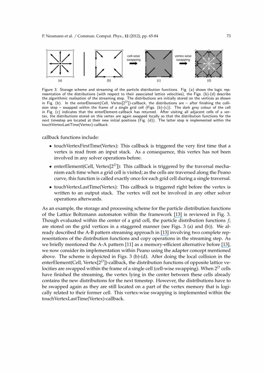
Figure 3: Storage scheme and streaming of the particle distribution functions. Fig. (a) shows the logic rep-resentation of the distributions (with respect to their associated lattice velocities), the Figs. (b)-(d) describethe algorithmic realisation of the streaming step. The distributions are initially stored on the vertices as shownin Fig. (b). In the enterElement(Cell, Vertex[2D ])-callback, the distributions are – after finishing the colli-sion step – swapped within the frame of a single grid cell (Figs. (b)-(c)). The dark grey colour of the cellin Fig. (c) indicates that the enterElement-callback has returned. After visiting all adjacent cells of a ver-tex, the distributions stored on this vertex are again swapped locally so that the distribution functions for thenext timestep are located at their new initial positions (Fig. (d)). The latter step is implemented within thetouchVertexLastTime(Vertex)-callback.

callback functions include:

• touchVertexFirstTime(Vertex): This callback is triggered the very first time that avertex is read from an input stack. As a consequence, this vertex has not beeninvolved in any solver operations before.

• enterElement(Cell, Vertex[2D]): This callback is triggered by the traversal mecha-nism each time when a grid cell is visited; as the cells are traversed along the Peanocurve, this function is called exactly once for each grid cell during a single traversal.

• touchVertexLastTime(Vertex): This callback is triggered right before the vertex iswritten to an output stack. The vertex will not be involved in any other solveroperations afterwards.

As an example, the storage and processing scheme for the particle distribution functionsof the Lattice Boltzmann automaton within the framework [13] is reviewed in Fig. 3.Though evaluated within the center of a grid cell, the particle distribution functions fi

are stored on the grid vertices in a staggered manner (see Figs. 3 (a) and (b)). We al-ready described the A-B pattern streaming approach in [13] involving two complete rep-resentations of the distribution functions and copy operations in the streaming step. Aswe briefly mentioned the A-A pattern [11] as a memory-efficient alternative before [13],we now consider its implementation within Peano using the adapter concept mentionedabove. The scheme is depicted in Figs. 3 (b)-(d). After doing the local collision in theenterElement(Cell, Vertex[2D])-callback, the distribution functions of opposite lattice ve-locities are swapped within the frame of a single cell (cell-wise swapping). When 2D cellshave finished the streaming, the vertex lying in the center between these cells alreadycontains the new distributions for the next timestep. However, the distributions have tobe swapped again as they are still located on a part of the vertex memory that is logi-cally related to their former cell. This vertex-wise swapping is implemented within thetouchVertexLastTime(Vertex)-callback.

74 P. Neumann et al. / Commun. Comput. Phys., 12 (2012), pp. 65-84

4 Lattice Boltzmann–Navier-Stokes coupling

Having reviewed the Lattice Boltzmann and the Navier-Stokes approach as well as thebasic principles of the Peano, we now discuss our coupling approach of the two methodswithin the framework.

The coupling of Lattice Boltzmann and Navier-Stokes systems requires the mappingof the respective unknowns

fi,ρLB,uLB↔ pNS,uNS.

As the reconstruction of one set of these variables necessitates interpolation depending onthe structural pattern of the underlying grids, the setup and positioning of the degrees offreedom for both fluid solvers is pointed out in Section 4.1. Subsequently, in Sections 4.2and 4.3, the mappings fi,ρ

LB,uLB → pNS,uNS and pNS,uNS → fi,ρLB,uLB are described in

detail.

4.1 Grid topology

In order to explain our coupling strategy, we restrict ourselves to a regular two-dimen-sional Cartesian grid. With the main feature of the Peano framework lying in adaptiveCartesian grids based on space-trees in arbitrary dimensions [5], note that our methodcan also be applied in an identical fashion to the adaptive counterparts of the describedsolvers for both 2D and 3D simulations.

The finite element implementation of the Navier-Stokes equation stores its velocityvalues uNS and the pressure pNS in a staggered manner on the grid [14] (see Fig. 4 onthe left). The velocity vectors are computed on the grid vertices whereas the pressure isstored in the center of every grid cell. The degrees of freedom of the Lattice Boltzmannautomaton, that is the particle distribution functions fi, are also evaluated in the cellcenter (see Fig. 4 on the right).

As a part of the fluid domain shall be computed by Lattice Boltzmann and anotherpart by Navier-Stokes, both solvers require valid boundary data for their simulations atthe interface between the respective subdomains. Our solution to this issue is depictedin Fig. 5. For the Lattice Boltzmann method, the distribution functions that would havebeen streamed from the Navier-Stokes domain into the Lattice Boltzmann domain needto be constructed in a suitable manner. We solve this by surrounding the Lattice Boltz-mann subdomain by an additional layer of cells; although being completely evaluated by

Figure 4: Storage pattern for both solvers. Left: Navier-Stokes solver. Right: Lattice Boltzmann solver.

P. Neumann et al. / Commun. Comput. Phys., 12 (2012), pp. 65-84 75

����������������������������������������������������������������������������������������������������

����������������������������������������������������������������������������������������������������

����������������������������������������������������������������������������������������������������

����������������������������������������������������������������������������������������������������

���

���

���

���

����������������������������������������

���������������������

���

NSoverlap overlap

Navier−Stokes Lattice Boltzmann

LB

����

����

����

����

����

����

����

��

����

f Lattice Boltzmann

f overlap

i

i

NS

NS

u Navier−Stokes

u overlap

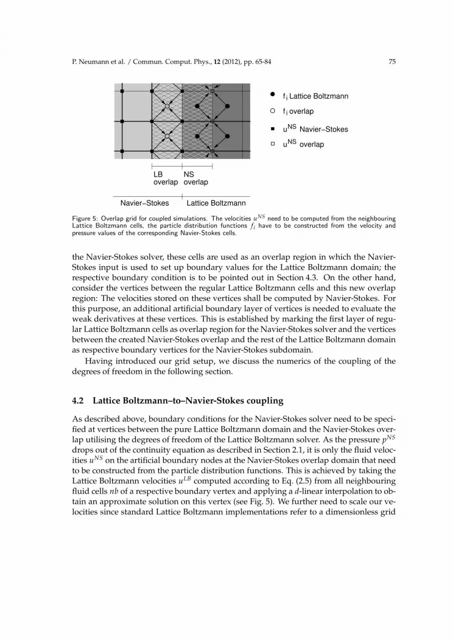
Figure 5: Overlap grid for coupled simulations. The velocities uNS need to be computed from the neighbouringLattice Boltzmann cells, the particle distribution functions fi have to be constructed from the velocity andpressure values of the corresponding Navier-Stokes cells.

the Navier-Stokes solver, these cells are used as an overlap region in which the Navier-Stokes input is used to set up boundary values for the Lattice Boltzmann domain; therespective boundary condition is to be pointed out in Section 4.3. On the other hand,consider the vertices between the regular Lattice Boltzmann cells and this new overlapregion: The velocities stored on these vertices shall be computed by Navier-Stokes. Forthis purpose, an additional artificial boundary layer of vertices is needed to evaluate theweak derivatives at these vertices. This is established by marking the first layer of regu-lar Lattice Boltzmann cells as overlap region for the Navier-Stokes solver and the verticesbetween the created Navier-Stokes overlap and the rest of the Lattice Boltzmann domainas respective boundary vertices for the Navier-Stokes subdomain.

Having introduced our grid setup, we discuss the numerics of the coupling of thedegrees of freedom in the following section.

4.2 Lattice Boltzmann–to–Navier-Stokes coupling

As described above, boundary conditions for the Navier-Stokes solver need to be speci-fied at vertices between the pure Lattice Boltzmann domain and the Navier-Stokes over-lap utilising the degrees of freedom of the Lattice Boltzmann solver. As the pressure pNS

drops out of the continuity equation as described in Section 2.1, it is only the fluid veloc-ities uNS on the artificial boundary nodes at the Navier-Stokes overlap domain that needto be constructed from the particle distribution functions. This is achieved by taking theLattice Boltzmann velocities uLB computed according to Eq. (2.5) from all neighbouringfluid cells nb of a respective boundary vertex and applying a d-linear interpolation to ob-tain an approximate solution on this vertex (see Fig. 5). We further need to scale our ve-locities since standard Lattice Boltzmann implementations refer to a dimensionless grid

76 P. Neumann et al. / Commun. Comput. Phys., 12 (2012), pp. 65-84

with unit meshsize and unit timesteps:

uNS=1

2D ∑cells nb

(

uLBnb ·

dx

dt

)

. (4.1)

4.3 Navier-Stokes–to–Lattice Boltzmann coupling

While scaled interpolation is sufficient to provide boundary data for the Navier-Stokesdomain, this is not the case when moving from the Navier-Stokes to the Lattice Boltz-mann system. The reason for this is that the information provided on the coarser macro-scale only represents a subset of the information which is present on the mesoscale. Ingeneral, the number of particle distribution functions Q (e.g. Q=9 for the D2Q9 model)exceeds the number of unknowns D+1 of the Navier-Stokes system. However, the equi-librium states f

eqi (ρ,u) of the system can be uniquely described by the macroscopic quan-

tities u and ρ. Hence, we first split the distribution functions in an equilibrium and non-equilibrium part,

fi = feqi (ρLB,uLB)+ f

neqi , i=1,··· ,Q. (4.2)

The quantities ρLB and uLB can be determined by direct injection and d-linear interpola-tion (see Fig. 5) from the Navier-Stokes variables pNS and uNS, including a pressure-to-density conversion according to Eq. (2.27) and a respective rescaling as mentioned in theprevious section. One further problem is caused by the macroscopic pressure pNS whichis only known up to a certain constant; the constant itself may vary between differentsimulation setups and even between different timesteps. In order to uniquely determinea valid density expression from the pressure, we follow the method from [12] where theconstant is chosen to be the average pressure over the interface in every timestep. In ourcase this implies computing the mean pressure pNS over all cells in the Lattice Boltzmannoverlap region and setting

ρLB =ρLB0 ·(

pNS− pNS

c2s

+1

)

(4.3)

with the dimensionless reference density ρLB0 =1.

Still, the non-equilibrium parts in Eq. (4.2) need to be determined. Latt et al. [12]introduce further approximations to the terms f

neqi in the Chapman-Enskog expansion

and derive an explicit relation between the non-equilibrium parts and the velocity gra-dients. These approximations comprise a neglection of spatial and temporal derivativesof the non-equilibrium parts and a restriction to a first-order velocity approximation ofthe equilibrium functions f

eqi . However, especially in case of non-stationary flows or in

the first timesteps of a Lattice Boltzmann simulation, where the system initially needs toreach a stable state, spatial and temporal variations in the non-equilibrium parts neces-sarily need to occur. Besides, a second-order accurate solution with respect to the flowvelocity u might be preferable.

P. Neumann et al. / Commun. Comput. Phys., 12 (2012), pp. 65-84 77

Therefore, we follow a different approach for the construction of the non-equilibriumdistributions f

neqi . As mass, momentum (see Eq. (2.13) and (2.14)) and viscous stresses

have to be conserved at the interface between the two solver regions, we get the followingconstraints for the non-equilibrium parts:

∑i

fneqi =0,

∑i

fneqi ciα

=0, for all α∈{1,··· ,D},

∑i

fneqi ciα

ciβ=− 2ν

2− 1τ

(

∂xβuα+∂xα uβ

)

, for all {α,β∈{1,··· ,D} : α≤β}, (4.4)

where the latter equation results from the insertion of the BGK collision operator intoEq. (2.28). Note that this particular choice of the collision operator is only made for sim-plicity. Other collision operators might as well be used at this point; however, besidechanges in the Chapman-Enskog expansion, the properties of the linear system of sideconstraints might change affecting the following reconstruction procedure of the non-equilibrium parts.

Having 1+D+D(D+1)/2 = (D+1)(D+2)/2 independent conditions for the non-equilibrium parts (for 2D: 6 conditions), we still have an under-determined system forf

neqi . As deviations from the equilibrium state are typically very small in a fluid at contin-

uum scale, we choose to minimise the non-equilibrium parts in a certain sense to obtaina fully determined system of non-equilibrium deviations f

neqi . Therefore, let

g( f neq)=Q

∑i=1

Q

∑j=i

gij fneqi f

neqj +

Q

∑i=1

gi fneqi +g0 (4.5)

be a second order polynomial function in f neq. Then, we use those variables fneqi which

minimise g such that the side constraints from Eq. (4.4) are fulfilled. Thus, for a givenfunction g( f neq), we solve

minf neq∈RQ

g( f neq) such that

∑i

fneqi =0,

∑i

fneqi ciα

=0, for all α∈{1,··· ,D},

∑i

fneqi ciα

ciβ=− 2ν

2− 1τ

(

∂xβuα+∂xα uβ

)

, for all {α,β∈{1,··· ,D} : α≤β}. (4.6)

Possible choices for g( f neq) are the squared L2-norm

g( f neq) :=‖ f neq‖22=∑

i

fneq2

i , (4.7)

78 P. Neumann et al. / Commun. Comput. Phys., 12 (2012), pp. 65-84

an expression representing an approximation for the order of the local Knudsen number(we will refer to this as the “squared Knudsen-norm”)

g( f neq) :=∑i

(

fneqi

feqi (ρLB,uLB)

)2

, (4.8)

or an “approximate squared Knudsen-norm” approximating the equilibrium distributionin the const-density low-velocity limit f

eqi ≈ f

eqi (ρLB

0 ,~0)=wi:

g( f neq) :=∑i

(

fneqi

wi

)2

. (4.9)

The restriction to functions lying in the space of second order polynomials is chosenfor the sake of simplicity; for second order polynomials, the minimisation problem de-scribed above leads to a linear system of equations for the corresponding Lagrange mul-tipliers and can uniquely be solved if this system is non-degenerated, i.e. its matrixE∈R

(D+1)(D+2)/2×(D+1)(D+2)/2 has full rank. For positive coefficients gii>0 of the minimi-sation polynomial, the matrix E becomes symmetric positive definite and the uniquenessof the solution is proven. For the proof of this statement, see the appendix. The costfunctions defined by Eqs. (4.7) and (4.9) have the advantage that the matrix E is knowna priori and can easily be inverted. As a consequence, the solving of the small linearsystems in all Lattice Boltzmann overlap cells can be omitted and changed into a cheapmatrix-vector multiplication.

4.4 Algorithm

Having described the coupling method, the overall algorithm for coupled Lattice Boltz-mann–Navier-Stokes simulations shall be reviewed:

// choose and set minimisation function g(f^neq)

setMinimisationFunction();

// flag cells and vertices belonging to LB or NS domain

// or belonging to LB or NS overlap domain

setupDomainFlagging();

t=0;

while (t+dt < t_end)

// construct f_i=f_i^eq + f_i^neq in LB overlap region

constructPdfsInLatticeBoltzmannOverlap();

// solve one LB timestep in LB region

solveLatticeBoltzmannDomain();

P. Neumann et al. / Commun. Comput. Phys., 12 (2012), pp. 65-84 79

// compute velocities on vertices of artificial NS boundary

constructVelocitiesInNavierStokesOverlap();

// solve one NS timestep

solveNavierStokesDomain();

t=t+dt

end

5 Implementation

As the Peano framework provides both implementations of the finite element Navier-Stokes solver and the Lattice Boltzmann method, a coupling according to the descriptionsin Section 4 could easily be established. In this section, we present some details of theresulting code structure.

First, in order to provide both particle distribution functions and macroscopic quan-tities on the grid, the data structures for the vertices and cells were prepared such thatthey hold both Navier-Stokes and Lattice Boltzmann degrees of freedom at the sametime. By this, a dynamic change of the Lattice Boltzmann–Navier-Stokes domain parti-tioning becomes possible which might turn out as an advantage in case of (dynamically)adaptive simulation setups where one is interested in understanding flow phenomenaon different scales in different regions of the simulation domain. In order to combineboth solvers without introducing invasive dependencies between them, a new compo-nent “solver-coupling” was included in the Peano framework. This component extendsexisting adapters and allows for modifications of their callbacks during a grid traversal.As an example, instead of executing the Lattice Boltzmann algorithm on the whole grid,a simple extension was plugged in via the solver-coupling component delegating calls tothe Lattice Boltzmann solver only for the case that cells in the Lattice Boltzmann regionare visited; otherwise, the callbacks to the solver are suppressed. The original callbacksof the solver adapter do not need to be touched for this procedure; it is only the “couplingrule” (in this case: only touch Lattice Boltzmann cells) that needs to be implemented.

More complex rules for the original adapters can be plugged in the same way. Refer-ring to the algorithm in Sect. 4.4, the step constructPdfsInLatticeBoltzmannOverlap()

can for example be executed during the solving of the Lattice Boltzmann domain, that isduring the step solveLatticeBoltzmannDomain(). In the same fashion, the constructionof the velocities at the artificial Navier-Stokes boundary can be integrated into one ofthe grid traversals that are carried out by the Navier-Stokes solver. Compared to thestand-alone Navier-Stokes solver, the coupled algorithm only requires one additionalgrid traversal in the setup phase for the domain flagging and one additional traversalper timestep for solving the Lattice Boltzmann domain. As the number of grid traver-sals is one of the most important factors with respect to performance within Peano, oursolver-coupling approach thus only yields a minimal increase in grid traversals.

80 P. Neumann et al. / Commun. Comput. Phys., 12 (2012), pp. 65-84

Beside the extension and modification of existing adapters, the steering of the coupledsimulation needs to be established requiring knowledge of both solver algorithms. Thisissue is solved by using the concept of multiple inheritance. With each, the Navier-Stokesand the Lattice Boltzmann solver, containing a simulation class for steering and executingthe algorithmic steps of the respective solver, we let the coupled simulation class inheritfrom both steering classes. Having all the single algorithmic steps available in our newclass, we can reorder and adapt them according to our algorithm from Section 4.4.

6 Results

The coupling algorithm was tested in a two-dimensional channel flow. In all setups, theflow field was initialised with zero-velocity and constant pressure. For the coupling inthe Lattice Boltzmann overlap region, the “squared Knudsen-norm” was applied as acost function; as the other cost functions showed similar behaviour through all tests, westick to this minimisation function from now on.

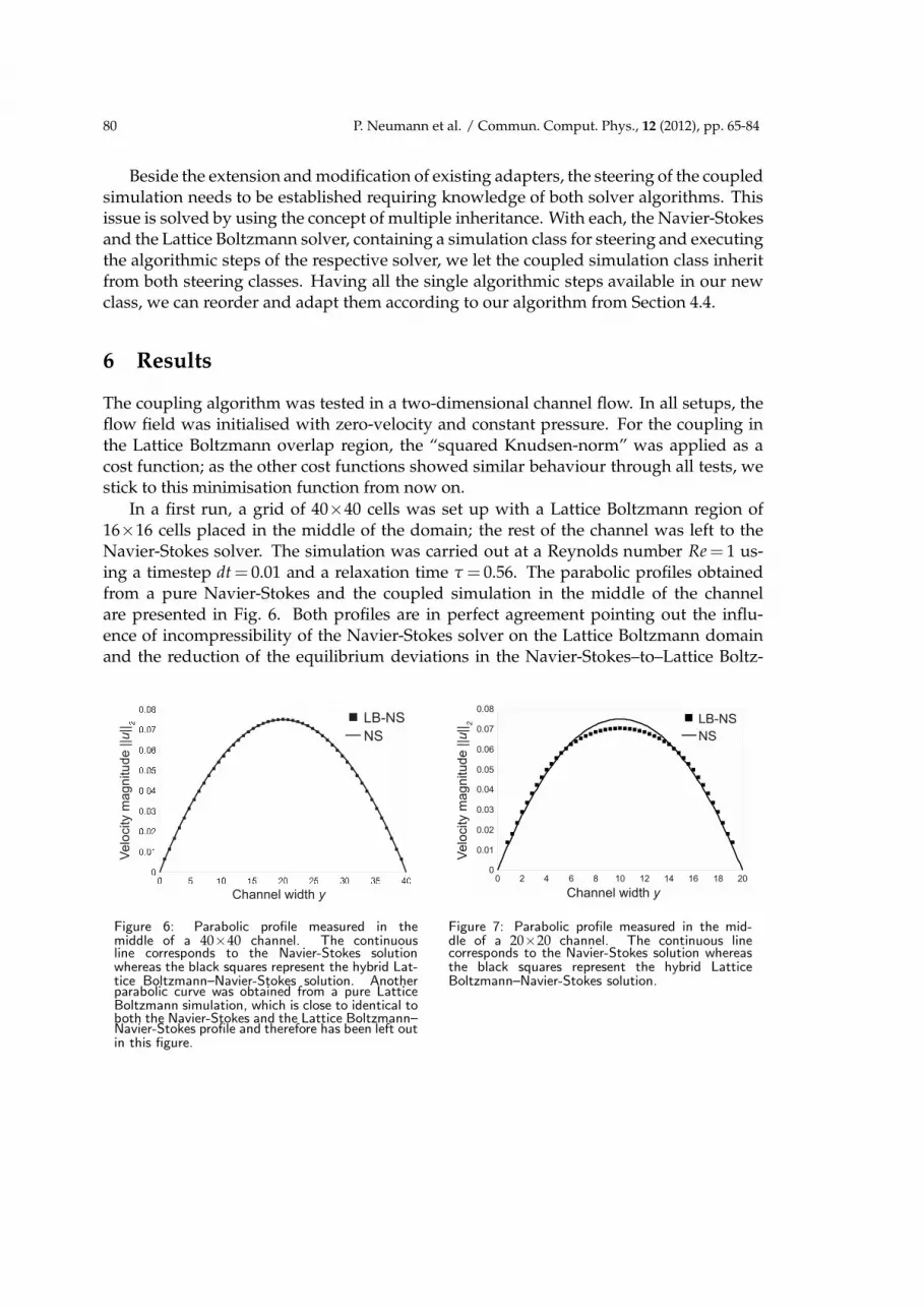
In a first run, a grid of 40×40 cells was set up with a Lattice Boltzmann region of16×16 cells placed in the middle of the domain; the rest of the channel was left to theNavier-Stokes solver. The simulation was carried out at a Reynolds number Re= 1 us-ing a timestep dt= 0.01 and a relaxation time τ = 0.56. The parabolic profiles obtainedfrom a pure Navier-Stokes and the coupled simulation in the middle of the channelare presented in Fig. 6. Both profiles are in perfect agreement pointing out the influ-ence of incompressibility of the Navier-Stokes solver on the Lattice Boltzmann domainand the reduction of the equilibrium deviations in the Navier-Stokes–to–Lattice Boltz-

Figure 6: Parabolic profile measured in themiddle of a 40×40 channel. The continuousline corresponds to the Navier-Stokes solutionwhereas the black squares represent the hybrid Lat-tice Boltzmann–Navier-Stokes solution. Anotherparabolic curve was obtained from a pure LatticeBoltzmann simulation, which is close to identical toboth the Navier-Stokes and the Lattice Boltzmann–Navier-Stokes profile and therefore has been left outin this figure.

Figure 7: Parabolic profile measured in the mid-dle of a 20×20 channel. The continuous linecorresponds to the Navier-Stokes solution whereasthe black squares represent the hybrid LatticeBoltzmann–Navier-Stokes solution.

P. Neumann et al. / Commun. Comput. Phys., 12 (2012), pp. 65-84 81

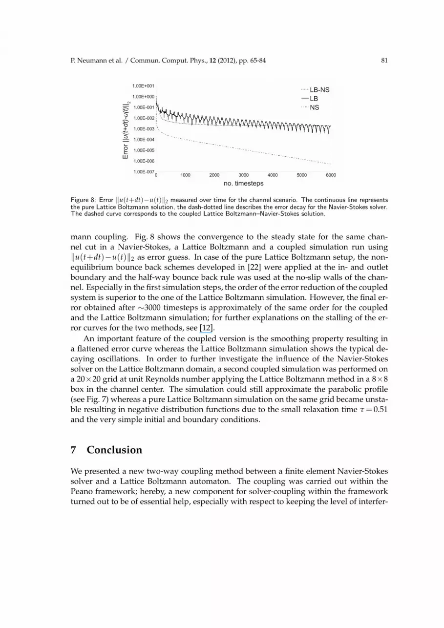
Figure 8: Error ‖u(t+dt)−u(t)‖2 measured over time for the channel scenario. The continuous line representsthe pure Lattice Boltzmann solution, the dash-dotted line describes the error decay for the Navier-Stokes solver.The dashed curve corresponds to the coupled Lattice Boltzmann–Navier-Stokes solution.

mann coupling. Fig. 8 shows the convergence to the steady state for the same chan-nel cut in a Navier-Stokes, a Lattice Boltzmann and a coupled simulation run using‖u(t+dt)−u(t)‖2 as error guess. In case of the pure Lattice Boltzmann setup, the non-equilibrium bounce back schemes developed in [22] were applied at the in- and outletboundary and the half-way bounce back rule was used at the no-slip walls of the chan-nel. Especially in the first simulation steps, the order of the error reduction of the coupledsystem is superior to the one of the Lattice Boltzmann simulation. However, the final er-ror obtained after ∼3000 timesteps is approximately of the same order for the coupledand the Lattice Boltzmann simulation; for further explanations on the stalling of the er-ror curves for the two methods, see [12].

An important feature of the coupled version is the smoothing property resulting ina flattened error curve whereas the Lattice Boltzmann simulation shows the typical de-caying oscillations. In order to further investigate the influence of the Navier-Stokessolver on the Lattice Boltzmann domain, a second coupled simulation was performed ona 20×20 grid at unit Reynolds number applying the Lattice Boltzmann method in a 8×8box in the channel center. The simulation could still approximate the parabolic profile(see Fig. 7) whereas a pure Lattice Boltzmann simulation on the same grid became unsta-ble resulting in negative distribution functions due to the small relaxation time τ= 0.51and the very simple initial and boundary conditions.

7 Conclusion

We presented a new two-way coupling method between a finite element Navier-Stokessolver and a Lattice Boltzmann automaton. The coupling was carried out within thePeano framework; hereby, a new component for solver-coupling within the frameworkturned out to be of essential help, especially with respect to keeping the level of interfer-

82 P. Neumann et al. / Commun. Comput. Phys., 12 (2012), pp. 65-84

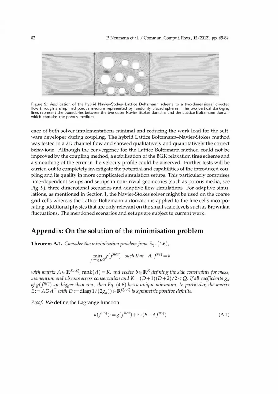
Figure 9: Application of the hybrid Navier-Stokes–Lattice Boltzmann scheme to a two-dimensional directedflow through a simplified porous medium represented by randomly placed spheres. The two vertical dark-greylines represent the boundaries between the two outer Navier-Stokes domains and the Lattice Boltzmann domainwhich contains the porous medium.

ence of both solver implementations minimal and reducing the work load for the soft-ware developer during coupling. The hybrid Lattice Boltzmann–Navier-Stokes methodwas tested in a 2D channel flow and showed qualitatively and quantitatively the correctbehaviour. Although the convergence for the Lattice Boltzmann method could not beimproved by the coupling method, a stabilisation of the BGK relaxation time scheme anda smoothing of the error in the velocity profile could be observed. Further tests will becarried out to completely investigate the potential and capabilities of the introduced cou-pling and its quality in more complicated simulation setups. This particularly comprisestime-dependent setups and setups in non-trivial geometries (such as porous media, seeFig. 9), three-dimensional scenarios and adaptive flow simulations. For adaptive simu-lations, as mentioned in Section 1, the Navier-Stokes solver might be used on the coarsegrid cells whereas the Lattice Boltzmann automaton is applied to the fine cells incorpo-rating additional physics that are only relevant on the small scale levels such as Brownianfluctuations. The mentioned scenarios and setups are subject to current work.

Appendix: On the solution of the minimisation problem

Theorem A.1. Consider the minimisation problem from Eq. (4.6),

minf neq∈RQ

g( f neq) such that A· f neq=b

with matrix A∈RK×Q, rank(A)=K, and vector b∈R

K defining the side constraints for mass,momentum and viscous stress conservation and K=(D+1)(D+2)/2<Q. If all coefficients gii

of g( f neq) are bigger than zero, then Eq. (4.6) has a unique minimum. In particular, the matrixE :=ADA⊤ with D :=diag(1/(2gii))∈R

Q×Q is symmetric positive definite.

Proof. We define the Lagrange function

h( f neq) := g( f neq)+λ·(b−A f neq) (A.1)

P. Neumann et al. / Commun. Comput. Phys., 12 (2012), pp. 65-84 83

with Lagrange multipliers λ∈RK. Differentiating h( f neq) with respect to f

neqi yields:

∂ fneqi

h( f neq)=2gii fneqi +

(

gi+i−1

∑j=1

gji+Q

∑j=i+1

gij

)

−∑k

λk Aki, i∈{1,··· ,Q}. (A.2)

Requiring a vanishing gradient for the Lagrange function leads to:

1

2gii∑

k

λk Aki = fneqi +

1

2gii

(

gi+i−1

∑j=1

gji+Q

∑j=i+1

gij

)

, i∈{1,··· ,Q}. (A.3)

Multiplying the equation system from Eq. (A.3) with the matrix A results in E·λ=r withE defined as above and the right hand side r∈R

K given by

rk :=bk+Q

∑i=1

Aki

2gii

(

gi+i−1

∑j=1

gji+Q

∑j=i+1

gij

)

, k∈{1,··· ,K}. (A.4)

The symmetry of E=ADA⊤ is trivial. For the positive definiteness, consider

x⊤Ex=K

∑k=1

xk

Q

∑i=1

Aki1

2gii

K

∑j=1

Ajixj =Q

∑i=1

(

K

∑k=1

Akixk

)2

(A.5)

for any non-zero vector x∈RK. As rank(A)=K, there is at least one term (∑K

k=1 Akixk)2>0;

thus, it isx⊤Ex>0 ∀x∈R

K\{~0}. (A.6)

This completes the proof.

References

[1] P. Albuquerque, D. Alemani, B. Chopard, and P. Leone. A Hybrid Lattice Boltzmann FiniteDifference Scheme for the Diffusion Equation. Int. J. Mult. Comp. Eng., 4(2):209–219, 2006.

[2] M. J. Berger and P. Collela. Local adaptive mesh refinement for shock hydrodynamics. J.Comput. Phys., 82:64–84, 1989.

[3] M. J. Berger and J. Oliger. Adaptive mesh refinement for hyperbolic partial differential equa-tions. J. Comput. Phys., 53:484–512, 1984.

[4] P. L. Bhatnagar, E. P. Gross, and M. Krook. A model for collision processes in gases. I. Smallamplitude processes in charged and neutral one-component systems. Phys. Rev., 94(3):511–525, 1954.

[5] H.-J. Bungartz, M. Mehl, T. Neckel, and T. Weinzierl. The PDE framework Peano applied tofluid dynamics: An efficient implementation of a parallel multiscale fluid dynamics solveron octree-like adaptive Cartesian grids. Comput. Mech., 46(1):103–114, June 2010. Publishedonline.

[6] S. Chapman and T. G. Cowling. The Mathematical Theory of Nonuniform Gases. CambridgeUniversity Press, London, 1960.

84 P. Neumann et al. / Commun. Comput. Phys., 12 (2012), pp. 65-84

[7] B. Dunweg, U. D. Schiller, and A. J. Ladd. Statistical Mechanics of the Fluctuating LatticeBoltzmann Equation. Phys. Rev. E, 76(036704), 2007.

[8] S. Geller, M. Krafczyk, J. Tolke, S. Turek, and J. Hron. Benchmark computations based onLattice-Boltzmann, finite element and finite volume methods for laminar flows. Comput.Fluids, 35(8–9):888–897, 2006. Proceedings of the First International Conference for Meso-scopic Methods in Engineering and Science.

[9] G. Karniadakis, A. Beskok, and N. Aluru. Microflows and Nanoflows. Fundamentals andSimulation. Springer, New York, 2005.

[10] A. J. C. Ladd. Numerical simulations of particulate suspensions via a discretized Boltzmannequation. Part 1. Theoretical foundation. J. Fluid Mech., 271:285–309, 1994.

[11] J. Latt. Technical report: How to implement your DdQq dynamics with only q variables pernode (instead of 2q). 2007. Technical report.

[12] J. Latt, B. Chopard, and P. Albuquerque. Spatial Coupling of a Lattice Boltzmannfluid model with a Finite Difference Navier-Stokes solver, 2005. Published online,http://arxiv.org/pdf/physics/0511243v1.

[13] M. Mehl, T. Neckel, and P. Neumann. Navier-Stokes and Lattice-Boltzmann on octree-likegrids in the Peano framework. Int. J. Numer. Meth. Fluids, 65:67–86, 2011.

[14] T. Neckel. The PDE Framework Peano: An Environment for Efficient Flow Simulations.Verlag Dr. Hut, 2009.

[15] H. Sagan. Space-filling Curves. Springer-Verlag, New York, 1994.[16] S. Succi. The Lattice Boltzmann Equation for Fluid Dynamics and Beyond. Oxford Univer-

sity Press, New York, 2001.[17] M. Tij, M. Sabbane, and A. Santos. Nonlinear Poiseuille flow in a gas. Phys. Fluids, 10:1021–

1027, 1998.[18] F. J. Uribe and A. L. Garcia. Burnett description for plane Poiseuille flow. Phys. Rev. E,

60(4):4063–4078, Oct 1999.[19] T. Weinzierl. A Framework for Parallel PDE Solvers on Multiscale Adaptive Cartesian Grids.

Verlag Dr. Hut, 2009.[20] D. A. Wolf-Gladrow. Lattice-Gas Cellular Automata and Lattice Boltzmann Models: An

Introduction. Springer, 2000.[21] Y. Zheng, A. L. Garcia, and B. J. Alder. Comparison of kinetic theory and hydrodynamics for

Poiseuille flow. RAREFIED GAS DYNAMICS: 23rd International Symposium, 663(1):149–156, 2003.

[22] Q. Zou. and X. He. On pressure and velocity flow boundary conditions and bounceback forthe Lattice Boltzmann BGK model. Phys. Fluids, 9(6):1591–1598, 1997.