a concept exploration method for product family design
TRANSCRIPT
A Concept Exploration Method for Product Family Design
A Thesis
Presented to
the Academic Faculty
By
Timothy W. Simpson
In Partial Fulfillment
of the Requirements for the Degree of
Doctor of Philosophy in Mechanical Engineering
Georgia Institute of Technology
September 1998
Copyright © 1998 by Timothy W. Simpson
ii
A Concept Exploration Method for Product Family Design
Approved:
Farrokh Mistree, ChairProfessor, Mechanical Engineering
Janet K. AllenSenior Research Scientist, MechanicalEngineering
Jonathan S. ColtonProfessor, Mechanical Engineering
Russell G. HeikesAssociate Professor, Industrial and SystemsEngineering
William H. ReadProfessor, Public Policy
David W. RosenAssociate Professor, Mechanical Engineering
Daniel P. SchrageProfessor, Aerospace Engineering
Date Approved

iii
ACKNOWLEDGMENTS
“If I have seen far, it is because I have stood on the shoulders of giants.”
— Sir Isaac Newton
This statement is a testament to all of those who contributed, in one form or
another, to this research. Consequently, there are many I would like to acknowledge. To
begin, I would like to thank God for giving me the strength, perseverance, and ability to
achieve what I have done, and I would like to thank my family for their continual love,
support, and encouragement. I also extended my sincerest thanks to Sterling Odom for her
love and support throughout this process as well; she has provided immeasurable
inspiration and motivation to help me get through it all.
I would like to thank my committee members for their comments and suggestions.
In particular, I would like to say a special thanks to Dr. Russell Heikes for first alerting me
to kriging and for our many discussions on experimental designs and metamodeling, Dr.
William Read for several enlightening discussions on mass customization and the emerging
knowledge-based economy, and Dr. Jonathan Colton for his meticulous editorial comments
and feedback. A special thanks also goes to Dr. Kwok-Leung Tsui for his assistance and
interest in the kriging and experimental design study in Chapter 5. Thanks also to Dr. Dave
Rosen and Dr. Janet Allen for our countless interactions over the past four years. Finally, I
would like to thank my advisor, Farrokh Mistree; I cannot even begin to express the
gratitude I feel for all that he has done for me.
Thanks to my colleagues in the Systems Realization Laboratory (SRL) at the
Georgia Institute of Technology, particularly, Matt Bauer, Reid Bailey, and Scott

iv
McDermott. Thanks also to those in the SRL who have gone before me and were always
willing to lend a hand: Pat Koch, Jesse Peplinski, Kemper Lewis, Wei Chen, and Stewart
Coulter; I cherish the time we spent together. Also, special thanks to Gabriel Hernandez,
Zahed Siddique, Mark McIntosh, Marc McLean, Yao Lin, and Kiran Krishnapur for
sharing their thoughts and ideas for the future work section in Chapter 8.
I would like to thank Dr. Thomas Zang from the NASA Langley Research Center
for his interest in my research and for making my summer internship there possible.
During my brief stay, I am indebted to Dr. Tony Giunta for his helpful comments and
discussion about kriging and for letting me use, modify, and improve on his kriging code
so that I did not have to start from scratch. Furthermore, I extend my gratitude to Dr. John
J. Korte, Timothy M. Mauery, and Jack Dunn for all of their help and assistance with the
aerospike nozzle example in Chapter 4. Finally, I wish to acknowledge Bill Goffe for
making a copy of his simulated annealing algorithm available for use in the fitting portion
of my kriging code.
Special thanks to Jonathan Maier for his help with the universal electric motor
example in Chapter 6; without him, the example would have paled in comparison to what
we were able to accomplish. I also wish to acknowledge Douglas Dawson, David
Schooley, Dr. Rhett T. George (from Duke University), Gerry Rescigno, Dick Walter, Al
Lehnerd, and Henry Klein for their helpful comments and insight into the example.
For the Design of Experiments study in Chapter 5, I would like to acknowledge the
contributions of the following people who were kind enough to provide their own codes:
• Orthogonal array design generator: Dr. Art Owen, Department of Statistics,
Stanford University, Palo Alto, CA.
• Maximin Latin hypercube design generator: Kurt D. Palmer, Industrial and Systems
Engineering Department, Georgia Institute of Technology, Atlanta, GA.
v
• Optimal Latin hypercube design generator: Dr. Jeong-Soo Park, Statistics
Department, Chonnam National University, Korea.
• Orthogonal array-based Latin hypercube design generator: Dr. Boxin Tang,
Department of Mathematical Sciences, University of Memphis, Memphis, TN.
• Orthogonal Latin hypercube design generator: Kenny Qian Ye, Department of
Statistics, University of Michigan, Ann Arbor, MI.
• Hammersley Sample Sequence design generator: Dr. Urmila Diwekar, Engineering
and Public Policy, Carnegie Mellon University, Pittsburgh, PA.
Funding for this research has been provided through a Graduate Research
Fellowship from the National Science Foundation. Additional financial support was
received through a Presidential Fellowship and a Woodruff Teaching Fellowship awarded
by the Georgia Institute of Technology. Financial support from NSF Grant DMI-96-12327
is also acknowledged. The work on the aerospike nozzle example was supported by the
National Aeronautics and Space Administration under NASA Contract No. NAS1-19480
while in residence at the Institute for Computer Applications in Science and Engineering,
Mail Stop 403, NASA Langley Research Center, Hampton, VA 23681-0001. Finally, the
cost of computer time was underwritten by the Systems Realization Laboratory at the
Georgia Institute of Technology.

vi
TABLE OF CONTENTS
ACKNOWLEDGMENTS iii
TABLE OF CONTENTS vi
LIST OF TABLES xv
LIST OF FIGURES xix
NOMENCLATURE xxvi
SUMMARY xxxi
CHAPTER 1 FOUNDATIONS FOR PRODUCT FAMILY AND
PRODUCT PLATFORM DESIGN 1
1.1 FRAME OF REFERENCE: PRODUCT FAMILY AND PRODUCT
PLATFORM DESIGN 2
1.1.1 Engineering Examples of Successful Product Families 4
1.1.2 Opportunities in Product Family Design and Product
Platform Design 9
1.2 FOUNDATIONS FOR DESIGNING SCALABLE PRODUCT
PLATFORMS FOR A PRODUCT FAMILY 15
1.2.1 Decision-Based Design, the Decision Support Problem
Technique, and the Compromise Decision Support Problem 15
1.2.2 The Robust Concept Exploration Method 18
1.3 RESEARCH FOCUS IN THE DISSERTATION 21
1.3.1 Research Questions and Hypotheses in the Dissertation 21
vii
1.3.2 Contributions from the Research 25
1.4 OVERVIEW OF THE DISSERTATION 26
CHAPTER 2 A LITERATURE REVIEW: PRODUCT FAMILY
AND PRODUCT PLATFORM DESIGN, ROBUST
DESIGN, AND METAMODELING 31
2.1 WHAT IS PRESENTED IN THIS CHAPTER 32
2.2 PRODUCT FAMILY AND PRODUCT PLATFORM DESIGN
TOOLS AND METHODS 34
2.2.1 Attention Directing Tools for Product Family and Product
Platform Design 34
2.2.2 Product Platform Assessments and Cost Models 41
2.2.3 Engineering Methods for Product Family Design 45
2.3 ROBUST DESIGN 52
2.3.1 Implementation of Robust Design: Taguchi’s Method, in the
Robust Concept Exploration Method, and with Design
Capability Indices 56
2.3.2 Robust Design for Product Family Design: Scale Factors 64
2.4 METAMODELING TECHNIQUES 68
2.4.1 Limitations of Response Surface Approaches 73
2.4.2 The Kriging Approach to Metamodeling 75
2.4.3 Classical and Space Filling Experimental Designs 82
2.5 A LOOK BACK AND A LOOK AHEAD 90
CHAPTER 3 THE PRODUCT PLATFORM CONCEPT
EXPLORATION METHOD 92
3.1 OVERVIEW OF THE PPCEM AND RESEARCH HYPOTHESES 93
3.1.1 Step 1 - Create the Market Segmentation Grid 94
3.1.2 Step 2 - Classify Factors and Ranges 95
3.1.3 Step 3 - Build and Validate Metamodels 97
viii
3.1.4 Step 4 - Aggregate Product Platform Specifications 99
3.1.5 Step 5 - Develop Product Platform Portfolio 101
3.1.6 Infrastructure of the PPCEM 107
3.2 RESEARCH HYPOTHESES AND POSITS FOR THE PPCEM 108
3.2.1 Relationship of the Research Hypotheses to the RCEM 110
3.2.2 Supporting Posits for the Research Hypotheses 111
3.3 STRATEGY FOR VERIFICATION AND TESTING OF THE
RESEARCH HYPOTHESES 115
3.3.1 Testing Hypothesis 1 and Sub-Hypotheses 1.1-1.3 118
3.3.2 Testing Hypotheses 2 and 3 120
3.4 A LOOK BACK AND A LOOK AHEAD 121
CHAPTER 4 INITIAL KRIGING FEASIBILITY STUDY:
DESIGN OF AN AEROSPIKE NOZZLE 123
4.1 OVERVIEW OF KRIGING MODELING AND A 1-D EXAMPLE 124
4.2 AEROSPIKE NOZZLE DESIGN PROBLEM 130
4.2.1 Metamodeling of the Aerospike Nozzle Problem 134
4.2.2 Error Analysis of Response Surface and Kriging Models 136
4.2.3 Graphical Comparison of Response Surface and Kriging
Models 137
4.2.4 Optimization using the Response Surface and Kriging
Metamodels 140
4.2.5 Lessons Learned from the Aerospike Nozzle Example 143
4.3 A LOOK BACK AND A LOOK AHEAD 144
CHAPTER 5 THE UTILITY OF KRIGING AND SPACE
FILLING EXPERIMENTAL DESIGNS 145
5.1 OVERVIEW OF KRIGING/DOE STUDY AND PROBLEM
TESTBED 146
ix
5.1.1 Overview of Testbed Problems 148
5.1.2 Factors and Levels for Kriging/DOE Experiment 153
5.1.3 Experimental Design Choices for Test Problems 155
5.1.4 Responses for the Kriging/DOE Experiment 160
5.2 PRECURSORY KRIGING/DOE DATA ANALYSIS AND ANOVA 161
5.2.1 Analysis of Variance of Kriging/DOE Study 163
5.2.2 Correlation of Error Measures 164
5.3 TESTING HYPOTHESIS 2: THE UTILITY OF KRIGING 167
5.3.1 Effect of Correlation Function on Kriging Model Accuracy 168
5.3.2 Effects of Equation Type on Kriging Model Accuracy 171
5.4 TESTING HYPOTHESIS 3: THE UTILITY OF SPACE FILLING
EXPERIMENTAL DESIGNS 176
5.4.1 Comparison of Designs for Two Variable Problems 177
5.4.2 Comparison of Designs for 3 Factors 179
5.4.3 Comparison of Designs for 4 Factors 182
5.4.4 Lessons Learned from Experimental Design Study 185
5.5 A LOOK BACK AND A LOOK AHEAD 186
CHAPTER 6 DESIGN OF A FAMILY OF UNIVERSAL
ELECTRIC MOTORS 190
6.1 OVERVIEW OF THE UNIVERSAL MOTOR PROBLEM 192
6.1.1 Physical Description, Schematic, and Nomenclature for the
Universal Motor Problem 192
6.1.2 Relevant Analyses for Universal Motor Problem 195
6.2 STEPS 1 AND 2: CREATE MARKET SEGMENTATION GRID
AND CLASSIFY FACTORS FOR UNIVERSAL MOTOR
PLATFORM 206
6.3 STEP 4: AGGREGATE PRODUCT SPECIFICATIONS AND
FORMULATE UNIVERSAL MOTOR PLATFORM
COMPROMISE DSP 210
x
6.4 STEP 5: DEVELOP THE UNIVERSAL MOTOR PLATFORM 212
6.5 RAMIFICATIONS OF THE RESULTS OF THE ELECTRIC
MOTOR EXAMPLE PROBLEM 216
6.5.1 Development of a Benchmark Universal Motor Family 216
6.5.2 Comparison between the Benchmark Universal Motor
Family and the PPCEM Motor Family 219
6.5.3 Improvements to the PPCEM Motor Family and Lessons
Learned 221
6.6 A LOOK BACK AND A LOOK AHEAD 232
CHAPTER 7 DESIGN OF A FAMILY OF GENERAL AVIATION
AIRCRAFT 234
7.1 STEP 1: DEVELOPMENT OF THE MARKET SEGMENTATION
GRID 236
7.1.1 Overview of the General Aviation Aircraft Example Problem 236
7.1.2 Brief Overview of Aircraft Design 237
7.1.3 The Market Segmentation Grid for the GAA Example
Problem 241
7.2 STEP 2: GAA FACTOR CLASSIFICATION 244
7.3 STEP 3: BUILD AND VALIDATE METAMODELS 247
7.4 STEP 4: AGGREGATE PRODUCT SPECIFICATIONS AND
FORMULATE GAA PLATFORM COMPROMISE DSP 251
7.5 STEP 5: DEVELOP THE GAA PLATFORM PORTFOLIO 255
7.5.1 Results of the GAA Compromise DSP for the Family of
Aircraft 256
7.5.2 Instantiation of the Family of General Aviation Aircraft 259
7.6 VERIFICATION OF GAA PRODUCT PLATFORM RESULTS 262
7.6.1 GAA Product Platform Compromise DSP Verification 263
7.6.2 Comparisons of Kriging Predictions and GASP 265
7.6.3 Comparison of PPCEM Results to Benchmark Aircraft 266
xi
7.6.4 Product Variety Tradeoff Study 278
7.7 LESSONS LEARNED: A LOOK BACK AND A LOOK AHEAD 288
CHAPTER 8 CLOSURE: ACHIEVEMENTS AND
RECOMMENDATIONS 293
8.1 CLOSURE: ANSWERING THE RESEARCH QUESTIONS 294
8.2 ACHIEVEMENTS: REVIEW OF RESEARCH CONTRIBUTIONS 300
8.3 CRITICAL ANALYSIS: LIMITATIONS OF THE RESEARCH 302
8.4 RECOMMENDATIONS: AVENUES OF FUTURE WORK 308
8.4.1 Potential Avenues of Future Work in Metamodeling 308
8.4.2 Future Work in Product Family and Product Platform
Design 311
8.4.3 Additional Verification of the PPCEM and Kriging
Metamodels through the Concurrent Design of an Engine
Lubrication System 313
8.4.4 Configuration Design of Common Automotive Platforms 314
8.4.5 Integrated Product and Process Design of Product Families
and Mass Customized Goods 316
8.4.6 Product Family Mappings and “Ideality” Metrics 317
8.4.7 Modeling the Value of Reuse and Remanufacturing in a
Product Family 318
8.5 CONCLUDING REMARKS 320
APPENDIX A KRIGING ALGORITHMS AND SOURCE CODE 321
A.1 BUILDING, VALIDATING, AND IMPLEMENTING A KRIGING
MODEL 322
A.1.1 Building a Kriging Model 322
A.1.2 Validating a Kriging Model 323
A.1.3 Using a Kriging Model 325
A.2 KRIGING SOURCE CODE 326
xii
A.2.1 The mlefinder.f Algorithm 326
A.2.2 The krigit.f Algorithm 335
A.2.3 Kriging Algorithm README File 348
A.2.4 Sample Parameter and Data Input Files and Kriging Output 352
APPENDIX B EXPERIMENTAL DESIGN DESCRIPTIONS 354
B.1 CLASSICAL EXPERIMENTAL DESIGNS 355
B.1.1 Central Composite Designs 355
B.1.2 Box-Behnken Designs 356
B.2 SPACE FILLING EXPERIMENTAL DESIGNS 358
B.2.1 Random Latin Hypercubes 358
B.2.2 Random Orthogonal Arrays 359
B.2.3 IMSE Optimal Latin Hypercubes 360
B.2.4 Maximin Latin Hypercubes 361
B.2.5 Orthogonal-Array Based Latin Hypercubes 362
B.2.6 Uniform Designs 363
B.2.7 Orthogonal Latin Hypercubes 365
B.2.8 Hammersley Sequence 366
APPENDIX C A MINIMAX LATIN HYPERCUBE DESIGN
GENERATOR USING A GENETIC ALGORITHM 368
C.1 WHY A MINIMAX LATIN HYPERCUBE DESIGN? 369
C.2 A GENETIC ALGORITHM FOR GENERATING MINIMAX
LATIN HYPERCUBE DESIGNS 370
C.3 EXAMPLE MINIMAX LATIN HYPERCUBE DESIGNS AND
CONVERGENCE STUDIES 375
APPENDIX D KRIGING TESTBED PROBLEMS 380
D.1 DESIGN OF A TWO-BAR TRUSS 381
xiii
D.2 DESIGN OF A SYMMETRIC THREE-BAR TRUSS 382
D.3 DESIGN OF A HELICAL COMPRESSION SPRING 384
D.3.1 Shear Stress 386
D.3.2 Free Length 386
D.3.3 Preload Deflection 387
D.3.4 Combined Deflections 387
D.3.5 Deflection Requirement 387
D.3.6 Geometric Constraints 388
D.4 DESIGN OF A TWO-MEMBER FRAME 388
D.5 DESIGN OF A WELDED BEAM 391
D.5.1 Weld Stress 392
D.5.2 Bar Bending Stress 393
D.5.3 Bar Buckling Load 393
D.5.4 Bar Deflection 393
D.6 DESIGN OF A PRESSURE VESSEL 394
APPENDIX E SUPPLEMENTAL INFORMATION FOR
KRIGING/DOE STUDY 397
E.1 CULLING THE DATA TO REMOVE POTENTIAL OUTLIERS 398
E.1.1 STEP 1: Culling the Data Based on RMSE.RANGE 398
E.1.2 STEP 2: Culling the Data Based on MAX.RANGE 400
E.1.3 STEP 3: Culling the Data Based on CVRMSE.RANGE 402
E.2 ANALYSIS OF VARIANCE RESULTS 406
E.3 INTERACTION OF DOE AND NSAMP 410
APPENDIX F SUPPLEMENTAL INFORMATION FOR GAA
EXAMPLE PROBLEM 413
F.1 GAA DESIGN VARIABLE DESCRIPTION 414
xiv
F.2 GAA KRIGING METAMODELS: SAMPLE POINTS, RESPONSE
VALUES, AND FITTED MLE PARAMETERS 416
F.3 ANALYSIS OF VARIANCE OF GAA RESPONSE MEANS 422
F.4 ADDITIONAL DESIGN SCENARIOS FOR STUDY GAA
PRODUCT PLATFORM USING CDK FORMULATION 424
F.4.1 PPCEM Cdk Values for Design Scenarios 1-8 425
F.4.2 PPCEM Aircraft Instantiations 429
F.5 CONVERGENCE HISTORIES OF INDIVIDUALLY DESIGNED
BENCHMARK TWO, FOUR, AND SIX SEATER AIRCRAFT 430
F.6 GAA PRODUCT VARIETY TRADEOFF STUDY INFORMATION 432
F.6.1 Rank Ordering of Design Variables 432
F.6.2 Product Variety Tradeoff Study Results for Scenario 2 434
F.6.3 Product Variety Tradeoff Study Results for Scenario 3 438
F.7 SAMPLE GAA DSIDES FILES FOR PPCEM FAMILY 442
F.7.1 Sample DSIDES File: gasp.oa64.cdk.s1h.dat 442
F.7.2 Sample DSIDES File: gasp.oa64.cdk.s1h.f 443
F.8 SAMPLE GAA DSIDES FILES FOR BENCHMARK AIRCRAFT 461
F.8.1 Sample DSIDES File: gasp5s3.dat 461
F.8.2 Sample DSIDES File: gasp5s3lo.f 462
REFERENCES 467
VITA 484
xv
LIST OF TABLES
Table 1.1 Product Family Examples: Approach and Available Support 13
Table 1.2 Relationship Between Hypotheses and Dissertation Sections 25
Table 2.1 Summary of Correlation Functions 78
Table 2.2 Error Measures for Kriging Metamodels 81
Table 3.1 Relationship Between Hypothesis Testing and Chapters 117
Table 4.1 Sample Points for 1-D Example 124
Table 4.2 Error Analysis of One Variable Example 130
Table 4.3 Model Diagnostics of Response Surface Models 135
Table 4.4 Theta Parameters for Kriging Models of Aerospike Nozzle 136
Table 4.5 Error Analysis of Aerospike Nozzle Approximation Models 137
Table 4.6 Aerospike Nozzle Optimization Problem Formulations 141
Table 4.7 Aerospike Nozzle Optimization Results Using Metamodels 142
Table 5.1 Factors and Level for Kriging/DOE Study 154
Table 5.2 Experimental Designs for Two Factor Test Problems 157
Table 5.3 Experimental Designs for Three Variable Test Problems 158
Table 5.4 Experimental Designs for Four Variable Test Problems 159
Table 5.5 Additional Random Points Used to Assess Model Accuracy 161
Table 5.6 Kriging Test Problem Model Summary 161
Table 5.7 Summary of ANOVA Results for Kriging/DOE Study 163
Table 5.8 Summary of Equations Accurately Modeled by Kriging 174
Table 6.1 Nomenclature for Universal Motors 194
Table 6.2 Constraints for Universal Motor Product Family 209
xvi
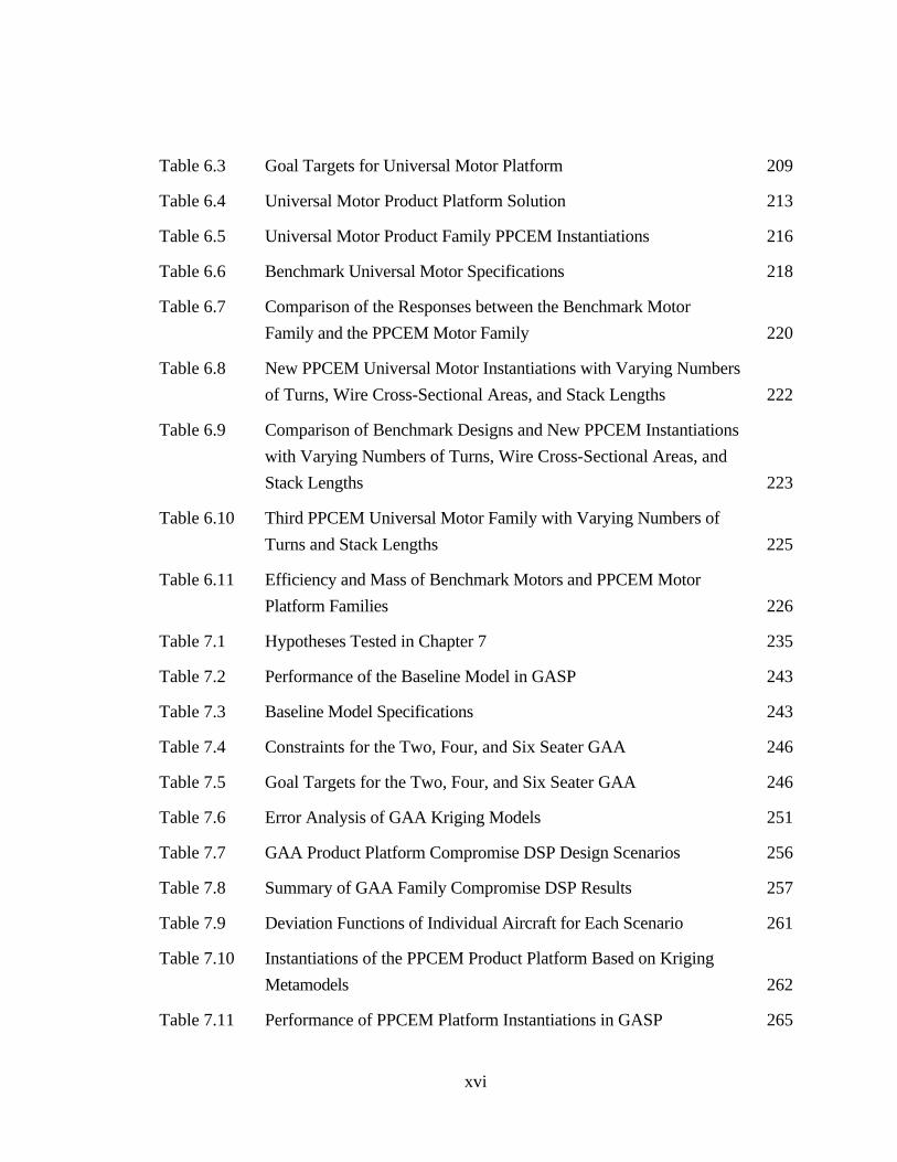
Table 6.3 Goal Targets for Universal Motor Platform 209
Table 6.4 Universal Motor Product Platform Solution 213
Table 6.5 Universal Motor Product Family PPCEM Instantiations 216
Table 6.6 Benchmark Universal Motor Specifications 218
Table 6.7 Comparison of the Responses between the Benchmark Motor
Family and the PPCEM Motor Family 220
Table 6.8 New PPCEM Universal Motor Instantiations with Varying Numbers
of Turns, Wire Cross-Sectional Areas, and Stack Lengths 222
Table 6.9 Comparison of Benchmark Designs and New PPCEM Instantiations
with Varying Numbers of Turns, Wire Cross-Sectional Areas, and
Stack Lengths 223
Table 6.10 Third PPCEM Universal Motor Family with Varying Numbers of
Turns and Stack Lengths 225
Table 6.11 Efficiency and Mass of Benchmark Motors and PPCEM Motor
Platform Families 226
Table 7.1 Hypotheses Tested in Chapter 7 235
Table 7.2 Performance of the Baseline Model in GASP 243
Table 7.3 Baseline Model Specifications 243
Table 7.4 Constraints for the Two, Four, and Six Seater GAA 246
Table 7.5 Goal Targets for the Two, Four, and Six Seater GAA 246
Table 7.6 Error Analysis of GAA Kriging Models 251
Table 7.7 GAA Product Platform Compromise DSP Design Scenarios 256
Table 7.8 Summary of GAA Family Compromise DSP Results 257
Table 7.9 Deviation Functions of Individual Aircraft for Each Scenario 261
Table 7.10 Instantiations of the PPCEM Product Platform Based on Kriging
Metamodels 262
Table 7.11 Performance of PPCEM Platform Instantiations in GASP 265
xvii
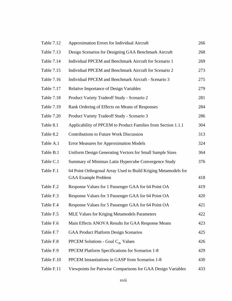
Table 7.12 Approximation Errors for Individual Aircraft 266
Table 7.13 Design Scenarios for Designing GAA Benchmark Aircraft 268
Table 7.14 Individual PPCEM and Benchmark Aircraft for Scenario 1 269
Table 7.15 Individual PPCEM and Benchmark Aircraft for Scenario 2 273
Table 7.16 Individual PPCEM and Benchmark Aircraft - Scenario 3 275
Table 7.17 Relative Importance of Design Variables 279
Table 7.18 Product Variety Tradeoff Study - Scenario 2 281
Table 7.19 Rank Ordering of Effects on Means of Responses 284
Table 7.20 Product Variety Tradeoff Study - Scenario 3 286
Table 8.1 Applicability of PPCEM to Product Families from Section 1.1.1 304
Table 8.2 Contributions to Future Work Discussion 313
Table A.1 Error Measures for Approximation Models 324
Table B.1 Uniform Design Generating Vectors for Small Sample Sizes 364
Table C.1 Summary of Minimax Latin Hypercube Convergence Study 376
Table F.1 64 Point Orthogonal Array Used to Build Kriging Metamodels for
GAA Example Problem 418
Table F.2 Response Values for 1 Passenger GAA for 64 Point OA 419
Table F.3 Response Values for 3 Passenger GAA for 64 Point OA 420
Table F.4 Response Values for 5 Passenger GAA for 64 Point OA 421
Table F.5 MLE Values for Kriging Metamodels Parameters 422
Table F.6 Main Effects ANOVA Results for GAA Response Means 423
Table F.7 GAA Product Platform Design Scenarios 425
Table F.8 PPCEM Solutions - Goal Cdk Values 426
Table F.9 PPCEM Platform Specifications for Scenarios 1-8 429
Table F.10 PPCEM Instantiations in GASP from Scenarios 1-8 430
Table F.11 Viewpoints for Pairwise Comparisons for GAA Design Variables 433
xviii
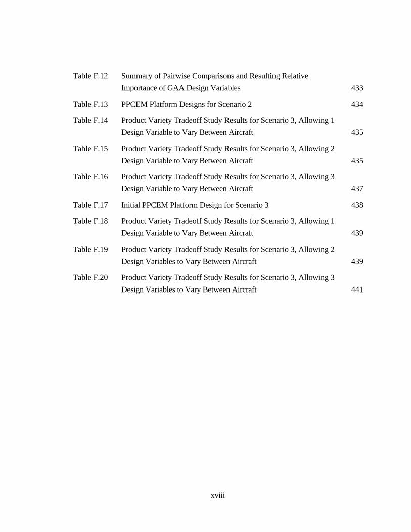
Table F.12 Summary of Pairwise Comparisons and Resulting Relative
Importance of GAA Design Variables 433
Table F.13 PPCEM Platform Designs for Scenario 2 434
Table F.14 Product Variety Tradeoff Study Results for Scenario 3, Allowing 1
Design Variable to Vary Between Aircraft 435
Table F.15 Product Variety Tradeoff Study Results for Scenario 3, Allowing 2
Design Variable to Vary Between Aircraft 435
Table F.16 Product Variety Tradeoff Study Results for Scenario 3, Allowing 3
Design Variable to Vary Between Aircraft 437
Table F.17 Initial PPCEM Platform Design for Scenario 3 438
Table F.18 Product Variety Tradeoff Study Results for Scenario 3, Allowing 1
Design Variable to Vary Between Aircraft 439
Table F.19 Product Variety Tradeoff Study Results for Scenario 3, Allowing 2
Design Variables to Vary Between Aircraft 439
Table F.20 Product Variety Tradeoff Study Results for Scenario 3, Allowing 3
Design Variables to Vary Between Aircraft 441
xix
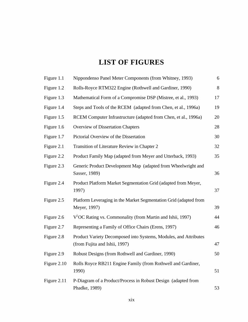
LIST OF FIGURES
Figure 1.1 Nippondenso Panel Meter Components (from Whitney, 1993) 6
Figure 1.2 Rolls-Royce RTM322 Engine (Rothwell and Gardiner, 1990) 8
Figure 1.3 Mathematical Form of a Compromise DSP (Mistree, et al., 1993) 17
Figure 1.4 Steps and Tools of the RCEM (adapted from Chen, et al., 1996a) 19
Figure 1.5 RCEM Computer Infrastructure (adapted from Chen, et al., 1996a) 20
Figure 1.6 Overview of Dissertation Chapters 28
Figure 1.7 Pictorial Overview of the Dissertation 30
Figure 2.1 Transition of Literature Review in Chapter 2 32
Figure 2.2 Product Family Map (adapted from Meyer and Utterback, 1993) 35
Figure 2.3 Generic Product Development Map (adapted from Wheelwright and
Sasser, 1989) 36
Figure 2.4 Product Platform Market Segmentation Grid (adapted from Meyer,
1997) 37
Figure 2.5 Platform Leveraging in the Market Segmentation Grid (adapted from
Meyer, 1997) 39
Figure 2.6 V2OC Rating vs. Commonality (from Martin and Ishii, 1997) 44
Figure 2.7 Representing a Family of Office Chairs (Erens, 1997) 46
Figure 2.8 Product Variety Decomposed into Systems, Modules, and Attributes
(from Fujita and Ishii, 1997) 47
Figure 2.9 Robust Designs (from Rothwell and Gardiner, 1990) 50
Figure 2.10 Rolls Royce RB211 Engine Family (from Rothwell and Gardiner,
1990) 51
Figure 2.11 P-Diagram of a Product/Process in Robust Design (adapted from
Phadke, 1989) 53
xx
Figure 2.12 Two Types of Robust Design (adapted from Chen, et al., 1996a) 55
Figure 2.13 A Motivating Example for Design Capability Indices 60
Figure 2.14 Implementation of Design Capability Indices for Robust Design
Applications 61
Figure 2.15 Compromise DSP Formulation with Design Capability Indices 63
Figure 2.16 Type III Robust Design: Scale Factors for Product Platforms 66
Figure 2.17 General Approach to Metamodeling (Koch, et al., 1997) 69
Figure 2.18 Techniques for Metamodeling 72
Figure 2.19 Sample Two-Variable Second-Order Response Surfaces (adapted
from Box and Draper, 1987) 74
Figure 2.20 Example Classical and Space Filling Experimental Designs 83
Figure 2.21 Central Composite Design 84
Figure 2.22 Box-Behnken Design 84
Figure 2.23 Latin Hypercube Design 86
Figure 2.24 Orthogonal Array Design 86
Figure 2.25 OA-Based Latin Hypercube 87
Figure 2.26 Orthogonal Latin Hypercube 87
Figure 2.27 Maximin Latin Hypercube 87
Figure 2.28 IMSE Optimal Latin Hypercube 88
Figure 2.29 Hammersley Design 88
Figure 2.30 Uniform Design 88
Figure 2.31 Example 9, 11, and 14 Point Minimax Latin Hypercubes 89
Figure 2.32 Pictorial Review of Chapter 2 and Preview of Chapter 3 91
Figure 3.1 Steps and Tools of the PPCEM 93
Figure 3.2 Step 1 - Create the Market Segmentation Grid 94
Figure 3.3 Step 2 - Factor Classification 95
xxi
Figure 3.4 Relationship of Scale Factors to the Market Segmentation Grid 97
Figure 3.5 Step 3 - Metamodel Development 98
Figure 3.6 Step 4 - Aggregating the Product Platform Specifications 100
Figure 3.7 Step 5 - Developing the Product Platform Portfolio 102
Figure 3.8 Estimating the Dissimilarity Index for a Product Family 104
Figure 3.9 Product Non-Commonality Versus Performance 105
Figure 3.10 Sample Product Variety Tradeoff Study 106
Figure 3.11 Infrastructure of the PPCEM 107
Figure 3.12 Relationships Between Hypotheses and RCEM Modifications 110
Figure 3.13 Pictorial Review of Chapter 3 and Preview of Chapter 4 122
Figure 4.1 One Variable Example Problem 125
Figure 4.2 MLE Objective Function for 1-D Example 127
Figure 4.3 One Variable Example of Response Surface and Kriging Models 129
Figure 4.4 VentureStar RLV with Aerospike Nozzle (Korte, et al., 1997) 131
Figure 4.5 Aerospike Components and Flow Field Characteristics (Korte, et
al., 1997) 131
Figure 4.6 Multidisciplinary Domain Decomposition for Aerospike Nozzle
(Korte, et al., 1997) 132
Figure 4.7 Nozzle Geometry Design Variables (Korte, et al., 1997) 133
Figure 4.8 Sample Points of 25 Point Orthogonal Array 134
Figure 4.9 Response Surface and Kriging Models for Thrust and Weight 138
Figure 4.10 Response Surface and Kriging Models for GLOW 139
Figure 5.1 Pictorial Overview of Kriging/DOE Study 147
Figure 5.2 Two-Bar Truss 150
Figure 5.3 Three-Bar Truss 150
Figure 5.4 Compression Spring 151
xxii
Figure 5.5 Two-Member Frame 151
Figure 5.6 Welded Beam 152
Figure 5.7 Pressure Vessel 152
Figure 5.8 Correlation Between RMSE.RANGE and MAX.RANGE 165
Figure 5.9 Correlation of RMSE.RANGE and CVRMSE.RANGE 166
Figure 5.10 Correlation of MAX.RANGE and CVRMSE.RANGE 167
Figure 5.11 Effect of Correlation Function Type on RMSE.RANGE 169
Figure 5.12 Effect of Correlation Function Type on MAX.RANGE 170
Figure 5.13 Effect of EQN of RMSE.RANGE for Testbed Problems 172
Figure 5.14 Effect of Equation Type on MAX.RANGE 173
Figure 5.15 Effect of 9 and 13 Point DOE on RMSE.RANGE 178
Figure 5.16 Effect of 9 and 13 Point DOE on MAX.RANGE 179
Figure 5.17 Effect of 13, 15, 21, and 23 Point DOE on RMSE.RANGE 180
Figure 5.18 Effect of 13, 15, 21 and 23 Point DOE on MAX.RANGE 182
Figure 5.19 Effect of 25 and 33 Point DOE on RMSE.RANGE 183
Figure 5.20 Effect of 25 and 33 Point DOE on MAX.RANGE 184
Figure 5.21 Pictorial Review of Chapter 5 and Preview of Chapter 6 188
Figure 6.1 Schematic of a Universal Motor (adapted from G.S.Electric, 1997) 193
Figure 6.2 Comparison of the Torque-Speed Characteristics of a Universal
Motor Rated at 1/4 Hp and 8000 rpm when Operating on AC and
DC Power Supplies (Martin, 1986) 195
Figure 6.3 An Idealized DC Motor (Chapman, 1991) 202
Figure 6.4 Model Geometry for a Universal Motor 204
Figure 6.5 Relative Permeability Versus Magnetizing Intensity for a Typical
Piece of Steel (Chapman, 1991) 205
Figure 6.6 Universal Motor Market Segmentation Grid 207
xxiii
Figure 6.7 P-Diagram for the Universal Motor Example 210
Figure 6.8 Universal Motor Product Platform Compromise DSP Formulation
for Use with OptdesX 211
Figure 6.9 Convergence Plots for the Universal Motor Product Platform 213
Figure 6.10 Compromise DSP Formulation for Instantiating the PPCEM
Platform for Use with OptdesX 215
Figure 6.11 Compromise DSP Formulation for Benchmark Universal Motor
Family for Use with OptdesX 217
Figure 6.12 Convergence Plots for 0.25 Nm Benchmark Motor 219
Figure 6.13 Pictorial Review of Chapter 6 and Preview of Chapter 7 233
Figure 7.1 Phases of Aircraft Design (Schrage, 1992) 238
Figure 7.2 GAA Market Segmentation Grid 241
Figure 7.3 Pictorial Representation of Baseline Aircraft 242
Figure 7.4 GAA Mission Profile 244
Figure 7.5 P-Diagram for GAA Example Problem 247
Figure 7.6 Product Array Approach for Constructing GAA Kriging Models 249
Figure 7.7 GAA Product Platform Compromise DSP Formulation 254
Figure 7.8 Convergence History of GAA Family C-DSP for Scenario 1 263
Figure 7.9 Convergence History for Scenarios 2 and 3 264
Figure 7.10 GAA Compromise DSP for Individual Aircraft 267
Figure 7.11 Graphical Comparison of Benchmark Aircraft and PPCEM Family
for Scenario 1 271
Figure 7.12 Graphical Comparison of Benchmark Aircraft and PPCEM Family
for Design Scenario 2, Priority Level 1 Only 274
Figure 7.13 Graphical Comparison of Benchmark Aircraft and PPCEM Family
for Design Scenario 3, Priority Level 1 Only 277
Figure 7.14 Scenario 2 Product Variety Tradeoff Study Results 282
xxiv
Figure 7.15 Pareto Plots for GAA Response Means 284
Figure 7.16 Scenario 3 Product Variety Tradeoff Study Results 287
Figure 8.1 Pictorial Overview of the Dissertation 295
Figure 8.2 The PPCEM as a Platform for Other Platform Design Methods 312
Figure A.1 Fitting a Kriging Model 322
Figure A.2 Optimization Using a Kriging Model 325
Figure B.1 Central Composite Design for 3 Factors 355
Figure B.2 Box-Behnken Design for 3 Factors 357
Figure B.3 Box-Behnken Design Matrices for 4, 5, and 6 Factors (from Box
and Behnken, 1960) 357
Figure B.4 Three Nine Point Latin Hypercube Designs for 2 Factors 359
Figure B.5 Orthogonal Array of Strength 2 for 3 Factors 360
Figure B.6 Optimal Latin Hypercube Designs for 2 Factors 361
Figure B.7 Maximin Latin Hypercube Designs for 2 Factors 362
Figure B.8 Six Point U Design and Latin Hypercube Design 363
Figure B.9 Uniform Designs for 2 Factors with 7, 9, and 11 Points 365
Figure B.10 Nine Point Orthogonal Latin Hypercube Designs for 2 Factors 366
Figure B.11 HSS Designs for 2 Factors with 7, 9, and 11 Points 367
Figure C.1 Genetic Algorithm for Creating Minimax Latin Hypercubes 371
Figure C.2 Expanding Concentric Circles of Equidistant Points 372
Figure C.3 Genetic Algorithm-Based Minimax Latin Hypercube Generator 374
Figure C.4 Convergence of 2 Factor mMlhd with 9 Sample Points 377
Figure C.5 Convergence of 2 Factor mMlhd with 14 Sample Points 377
Figure C.6 Convergence of 3 Factor mMlhd with 15 Sample Points 378
Figure C.7 Convergence of 3 Factor mMlhd with 23 Sample Points 378
Figure C.8 Convergence of 4 Factor mMlhd with 25 Sample Points 379
xxv
Figure C.9 Convergence of 4 Factor mMlhd with 41 Sample Points 379
Figure D.1 Two-Bar Truss 381
Figure D.2 Symmetric Three-Bar Truss 383
Figure D.3 Helical Compress Spring (from Siddall, 1982) 385
Figure D.4 Two-Member Frame 389
Figure D.5 Welded Beam 392
Figure D.6 Pressure Vessel 395
Figure E.1 Original Distribution of RMSE.RANGE of Data 399
Figure E.2 Resulting Distribution of RMSE.RANGE after Culling 400
Figure E.3 Distribution of MAX.RANGE of Culled Data Set 401
Figure E.4 Resulting Distribution of MAX.RANGE after Culling 402
Figure E.5 Distribution of CVRMSE.RANGE of Culled Data Set 403
Figure E.6 Distribution of CVRMSE.RANGE of Final Culled Data Set 404
Figure E.7 Distribution of RMSE.RANGE of Final Culled Data Set 405
Figure E.8 Distribution of MAX.RANGE of Final Culled Data Set 406
Figure E.9 Effect of DOE and Sample Size on RMSE.RANGE for the Two
Variable Problems 411
Figure E.10 Effect of DOE and Sample Size on RMSE.RANGE for the Three
Variable Problems 412
Figure E.11 Effect of DOE and Sample Size on RMSE.RANGE for the Four
Variable Problems 412
Figure F.1 Convergence of Individual Benchmark Aircraft - Scenario 1 431
Figure F.2 Convergence of Individual Benchmark Aircraft - Scenario 2 431
Figure F.3 Convergence of Individual Benchmark Aircraft - Scenario 3 432
xxvi
NOMENCLATURE
ANOVA Analysis of Variance
β Underlying constant in a kriging model
Cdk Design Capability Index
Control factor Design variables which can be freely specified by a designer
CVRMSE Cross Validation Root Mean Square Error
di+, d i
- Positive and negative deviation variables in compromise DSP
DBD Decision-Based Design
Derivative Product A specific instantiation of a product platform within a product family
which possesses unique form features and function(s) from other
members in the product family
DOE Design of Experiments
DSIDES Decision Support In the Design of Engineering Systems (computer
software for solving the compromise Decision Support Problem)
DSP Decision Support Problem
GAA General Aviation Aircraft
GASP General Aviation Synthesis Program
GRG Generalized Reduced Gradient algorithm in OptdesX optimization
software (Parkinson, et al., 1998)
IMSE Integrated Mean Square Error
JMP® Statistical analysis and experimental design software
Kriging Metamodeling technique from geostatistics which relies on the spatial
correlation of sample data to predict new values of a response, see,
e.g., (Cressie, 1993)
xxvii
LRL Lower Requirement Limit
Market
Segmentation Grid An attention directing tool used to map product platform leveraging
strategies within a product family
MAX Maximum absolute error
µ Mean value
Metamodel A “model of a model” which provides a surrogate approximation for
the actual response (Kleijnen, 1987)
MLE Maximum Likelihood Estimate
MSE Mean Square Error
MDO Multidisciplinary Design Optimization
NCI Non-Commonality Index
Noise factors Parameters in a system over which a designers has no control or are
too difficult or expensive to control
PDI Performance Deviation Index
Product Family A group of products which share common form features and
function(s), targeting one or multiple market niches
Product Platform The common set of design variables around which a family of
products can be developed. In more general terms, a product platform
is the common technological base from which a product family is
derived through modification and instantiation of the product platform
to target specific market niches.
PPCEM Product Platform Concept Exploration Method
Product Variant Synonym for derivative product
R Correlation matrix in a kriging model
R2, R2adj The ratio of the model sum of squares to the total sum of squares, and
that ratio adjusted for the number of parameters in the model
RCEM Robust Concept Exploration Method, see, e.g., (Chen, et al., 1996a)
xxviii
Response Performance parameter of the system, i.e., a system constraint or goal
RMSE Root Mean Square Error
RS Response surface
S-PLUS4® Statistical analysis software (Mathsoft, 1997)
Scalability The capability of a product platform to be “scaled,” “stretched,” or
“leveraged” to satisfy specific market niches
Scale factor A factor (i.e., design variable) around which a product platform can
be “scaled” or “stretched” to realize derivative products within a
product family
SN Signal-to-Noise ratio in robust design
σ Standard deviation
θk Spatial correlation parameters used to fit a kriging model
URL Upper Requirement Limit
x Design variable or control factor
y response value
ˆ y estimated response value
Z Deviation function in compromise DSP formulation
Variables used in Aerospike Nozzle Example in Chapter 4
a Thruster (starting) angle on the rocket nozzle
GLOW Gross Lift-Off Weight
h Base height of the rocket nozzle
l Base length of the rocket nozzle
Variables used in Kriging/DOE Study in Chapter 5
NSAMP Number of samples
CORFCN Correlation function
xxix
EQN Equation number
MAX.RANGE Maximum absolute error normalized by the sample range
RMSE.RANGE Root mean square error normalized by the sample range
Experimental Design Types
bxbnk Box-Behnken Design
CCD, ccdes Central Composite Design
CCF, ccfac Central Composite Face-Centered Design
CCI, ccins Central Composite Inscribed Design
hamss Hammersley Sampling Sequence Design
mnmxl Minimax Latin Hypercube
mxmnl Maximin Latin Hypercube
OA, oarry Orthogonal Array
oalhd Orthogonal Array-Based Latin Hypercube
oplhd IMSE Optimal Latin Hypercube
rnlhd Random Latin Hypercube
unifd Uniform Design
yelhd Orthogonal Latin Hypercube
Variables used in General Aviation Aircraft Example in Chapter 7
AF Engine Activity Factor
AR Aspect Ratio
CSPD Aircraft Cruise Speed
DOC Direct Operating Cost
DPRP Propeller Diameter
LDMAX Maximum Lift to Drag Ratio

xxx
NOISE Take-off Noise
PAX Number of Passengers
PURCH Aircraft Purchase Price
RANGE Maximum Cruise Range
ROUGH Ride Roughness Factor
VCRMX Maximum Cruise Speed
WEMP Aircraft Empty Weight
WFUEL Aircraft Fuel Weight
WL Wing Loading Estimate
WS Seat Width
(Variables used in the universal electric motor example are listed separately in Chapter 6)
xxxi
SUMMARY
Today’s competitive and highly volatile markets are redefining the way companies
do business. Companies are being faced with the challenge of providing as much variety
as possible for these markets with as little variety as possible between products.
Developing a family of products—a group of related products derived from a common
product platform—provides an efficient and effective means to realize sufficient product
variety to satisfy customer demands. Product families based on derivatives of a scalable
product platform are investigated in this dissertation. In particular, the Product Platform
Concept Exploration Method (PPCEM) is developed, presented, and tested as a Method
which facilitates the synthesis and Exploration of a common Product Platform Concept
which can be scaled into an appropriate family of products. The PPCEM consists of five
steps which prescribe how to formulate the problem and describe how it can be solved.
Finally, the PPCEM facilitates generating common product platform alternatives and their
corresponding product families but is not necessarily used to select one of them.
Testing and verification of the method occurs through two example problems:
• the design of a universal electric motor platform which is scaled around the stack
length of the motor to realize a family of motors capable of satisfying a variety of
torque and power requirements, and
• the design of a General Aviation aircraft platform which is scaled into two, four,
and six seat configurations to realize a family of aircraft capable of satisfying a
variety of performance and economic requirements.
Furthermore, indices of commonality and performance of a product family based on a
common, scalable product platform are proposed, enabling product variety tradeoff studies
to be performed. As a demonstration, the indices are employed in the General Aviation

xxxii
aircraft example to assess the compromise between commonality and performance of the
individual aircraft within the family.
In addition to developing a method to facilitate the design of a scalable product
platform for a product family, metamodeling techniques to facilitate concept exploration,
and the implementation of robust design within the PPCEM are investigated. Specifically,
the utility of kriging and space filling experimental designs for building inexpensive-to-run
surrogate approximations of deterministic computer analyses is examined. An initial 1-D
example is used first to familiarize the reader with the mathematics of kriging and the
differences between a kriging model and a response surface. Then a simple, yet realistic,
engineering example—the design of an aerospike nozzle—is used to compare and contrast
kriging models with second-order response surface models, the current standard for
building surrogate approximations in engineering design.
After the usefulness of kriging is demonstrated in the aerospike nozzle example, a
testbed of structural and mechanical engineering problems is introduced to test further the
utility of kriging and space filling experimental designs. Of the five correlation functions
studied for the kriging models, the Gaussian correlation function yields the most accurate
kriging models, on average, when building metamodels for the testbed of problems, and
the kriging models, in general, yield sufficiently accurate results for more than three
quarters of the functions investigated. Furthermore, the space filling and classical
experimental designs yield comparable results for the two variable problems in the testbed,
but the space filling designs tend to produce more accurate kriging models as the number of
variables increases and more so as the number of sample points increases. Finally, a
minimax Latin hypercube design also is developed in this dissertation specifically for use
with kriging metamodels; when compared to the other experimental designs in the problem
testbed, it is consistently among the best designs.

1
1. CHAPTER 1
FOUNDATIONS FOR PRODUCT FAMILY ANDPRODUCT PLATFORM DESIGN
The principal objective in this dissertation is to develop the Product Platform
Concept Exploration Method (PPCEM) to facilitate the design of a common scalable
product platform for a product family. As the title of this chapter implies, the foundations
for developing this method are presented here. The heart of the chapter lies in Section 1.3
wherein the research objectives, hypotheses, and contributions for the work are described;
this sets the stage for the chapters that follow, culminating in the development of the
PPCEM in Chapter 3. Sections 1.1 and 1.2 contain the motivation, foundation, and
context for investigating the proposed research and serve to establish context for the reader.
Specifically, in Section 1.1 the concepts of product family and product platform design are
introduced and defined, and opportunities for advancing this nascent research area are
identified. In Section 1.2, the foundations for the work—Decision-Based Design and the
Robust Concept Exploration Method—are presented. Finally, Section 1.4 contains an
overview of the dissertation.
2
1.1 FRAME OF REFERENCE: PRODUCT FAMILY AND PRODUCTPLATFORM DESIGN
Today’s competitive and highly volatile market is redefining the way companies do
business. “Customers can no longer be lumped together in a huge homogeneous market,
but are individuals whose individual wants and needs can be ascertained and fulfilled”
(Pine, 1993). Companies are being called upon to deliver better products faster and at less
cost for customers who are more demanding in a market which is characterized by words
such as mass customization and rapid innovation. Even government agencies like NASA
are re-examining the way they operate and do business, adopting slogans such as “better,
faster, cheaper.”
Erens (1997) refers to the market as a “buyer’s market” in which manufacturing
companies must satisfy individual customer requirements; he writes as follows:
“The sellers’ market of the fifties and sixties was characterized by high demand and
a relative shortage of supply. Firms produced large volumes of identical products,
supported by mass production techniques. ... The buyer’s market of the eighties
and beyond is forcing companies making specific high-volume products to
manufacture a growing range of products tailored to individual customer’s needs at
the cost of standard mass-produced goods.”
So why the growing concern for satisfying the individual customer? Stan Davis,
the person who coined the term mass customization, captures it best: “The more a company
can deliver customized goods on a mass basis relative to their competition, the greater is
their competitive advantage” (Davis, 1987). Simply stated, companies which offer
customized goods at minimal extra cost have a competitive advantage over those that do
not. Pine (1993) attributes the increasing attention on product variety and customer
demand to the saturation of the market and the need to improve customer satisfaction:
“Today, demand for new products frequently has to be diverted from older ones. It
is therefore important for new products to meet customer needs more completely, to

3
be of higher quality, and simply to be different from what is already in the
marketplace.”
Similar themes pervade the texts by Wortmann, et al., (1997) who examine industry’s
response in Europe to the “customer-driven” market, and Anderson (1997) who examines
the role of agile product development for mass customization.
This increasing need to distinguish and differentiate products from competitors is
further evidenced by Hollins and Pugh (1990):
"The customer now has plenty of choice for almost every product within a price
range. With this increased choice, consumers have become more aware of the good
and bad features of a product...they select the product that most closely fulfills their
opinion of being the best value for the money. This is not just price but a wide
range of non-price factors such as quality, reliability, aesthetics..."
Chinnaiah, et al. (1998) also examine the trend toward mass customized goods, citing more
demanding customers and market saturation as impetus for the shift. Uzumeri and
Sanderson (1997) state that “The emergence of global markets has fundamentally altered
competition as many firms have known it” with the resulting market dynamics “forcing the
compression of product development times and expansion of product variety.” The study
by Womack, et al. (1990) of the automobile industry in the 1980s provides just one of
numerous examples of this trend.
Since many companies typically design new products one at a time, Meyer and
Lehnerd (1997) have found that the focus on individual customers and products results in
“a failure to embrace commonality, compatibility, standardization, or modularization among
different products or product lines.” Similarly, Erens (1997) states that “If sales engineers
and designers focus on individual customer requirements, they feel that sharing
components compromises the quality of their products.” The end result is a
“mushrooming” or diversification of products and parts with proliferating variety and
4
costs. Mather (1995) states that “Rarely does the full spectrum of product offerings get
reviewed at one time to ensure it is optimal for the business.”
Consequently, companies are being faced with the challenge of providing as much
variety as possible for the market with as little variety as possible between products.
Toward this end, the approach advocated in this dissertation and by many strategic
marketing/management researchers and designers/engineers alike is to design and develop a
family of products with as much commonality between products as possible with minimal
compromise in quality and performance. Several engineering examples are presented in the
next section to provide context and foster a better understanding of the product family
concept and how product families have been successfully developed and realized.
Research opportunities in product family and product platform design then are discussed in
Section 1.1.2.
1 .1 .1 Engineering Examples of Successful Product Families
The following examples from Sony, Lutron, Nippondenso, Black & Decker,
Canon, and Rolls-Royce exemplify successful product families and have been studied as
such. Additional examples which might interest the reader include: Swiss army knives and
Swatch watches (Ulrich and Eppinger, 1995), Xerox copiers (Paula, 1997), Anderson
windows (Stevens, 1995), Hewlett-Packard printers (see, e.g., Lee, et al., 1993), the
Boeing 747 family of aircraft (see, e.g., Rothwell and Gardiner, 1990), and the Kodak
single use camera (see, e.g., Clark and Wheelwright, 1993).
Sony - The Sony Walkman
The design of the Sony Walkman is a classic example of managing the design of a product
family (Sanderson and Uzumeri, 1997). Sony first introduced the Walkman in 1979,
which has dominated the personal portable stereo market for over a decade, and has
remained the leader both technically and commercially despite fierce competition from

5
world-class competitors, e.g., Matushita, Toshiba, Sanyo and Sharp. Sony built all of
their Walkman models around key modules and platforms and used modular design and
flexible manufacturing to produce a wide variety of quality products at low cost.
Incremental design changes accounted for only 20-30 of the 250+ models Sony introduced
in the U.S. in the 1980s. “The remaining 85% of Sony's models were produced from
minor rearrangements of existing features and cosmetic redesigns of the external
case...topological changes [such as these] can be made with little cost or risk” (Sanderson
and Uzumeri, 1995). The basic mechanisms in each platform were refined continually
while following a disciplined and creative approach of focusing its families on clear design
goals while targeting models to distinct market segments.
Lutron - Electronic Lighting Control Systems
When engineers at Lutron design a new product line, they begin with a fairly standard
product with very few options (see, e.g., Spira, 1993). They then work with individual
customers to extend the product line until they eventually have a hundred or so models
which customers can purchase. Then engineering and production work together to
redesign the product line with 15-20 standardized components that can be configured into
the same hundred models from which customers could initially chose. Additional
customization work can be performed to meet individual customer requirements; in its
electronic lighting systems line, used in conference rooms, ballrooms, and hotel lobbies,
Lutron has rarely shipped the same system twice (Spira, 1993).
Nippondenso - Automotive Panel Meters
Nippondenso Co. Ltd. makes automotive components for Toyota, other Japanese car
makers, and car makers in other countries. They design their panel meters using a
combinatoric strategy as illustrated in Figure 1.1. A panel meter is composed of six parts
(in rare cases, only five), and in order to reduce inventory and production costs, each type
6
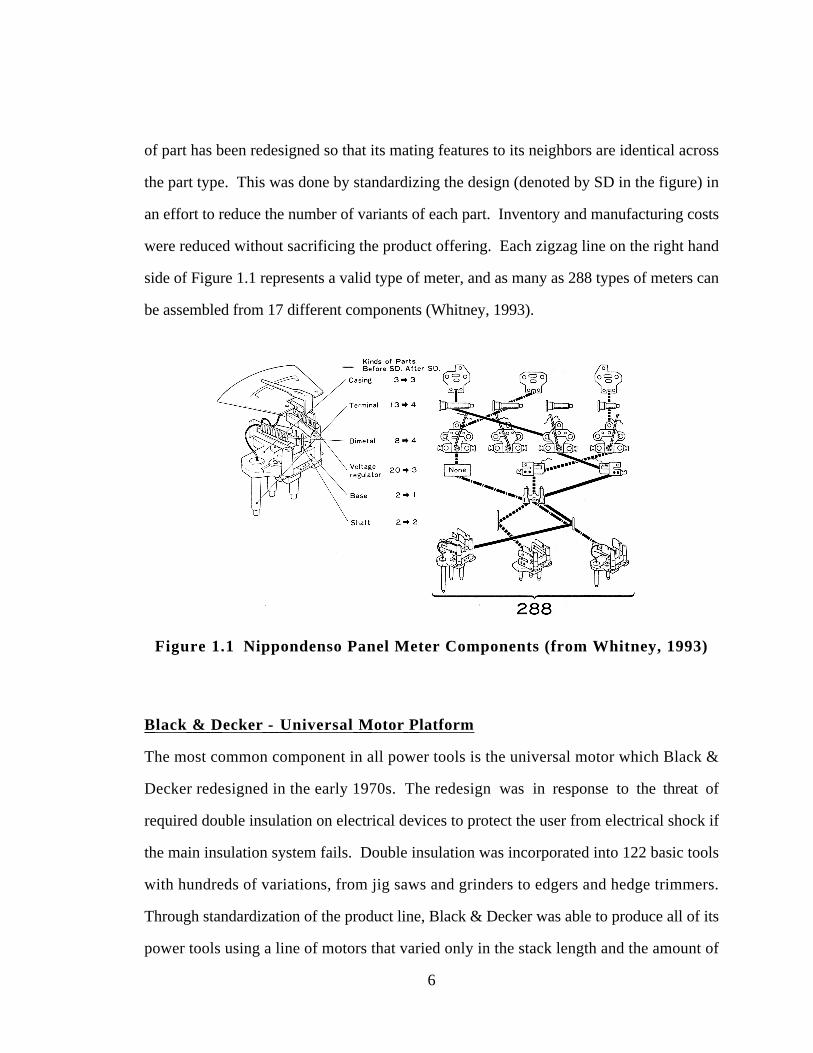
of part has been redesigned so that its mating features to its neighbors are identical across
the part type. This was done by standardizing the design (denoted by SD in the figure) in
an effort to reduce the number of variants of each part. Inventory and manufacturing costs
were reduced without sacrificing the product offering. Each zigzag line on the right hand
side of Figure 1.1 represents a valid type of meter, and as many as 288 types of meters can
be assembled from 17 different components (Whitney, 1993).
Figure 1.1 Nippondenso Panel Meter Components (from Whitney, 1993)
Black & Decker - Universal Motor Platform
The most common component in all power tools is the universal motor which Black &
Decker redesigned in the early 1970s. The redesign was in response to the threat of
required double insulation on electrical devices to protect the user from electrical shock if
the main insulation system fails. Double insulation was incorporated into 122 basic tools
with hundreds of variations, from jig saws and grinders to edgers and hedge trimmers.
Through standardization of the product line, Black & Decker was able to produce all of its
power tools using a line of motors that varied only in the stack length and the amount of
7
copper wrapped within the motor. As a result, all of the motors could be produced on a
single machine with stack lengths varying from 0.8 in to 1.75 in and power output ranging
from 60 to 650 watts. Furthermore, new designs were developed using standardized
components such as the redesigned motor, which allowed products to be introduced,
exploited and retired with minimal expense related to product development; see (Lehnerd,
1987) for additional information.
Canon - Copiers
Canon has successfully dominated the low volume end of the copier market since the mid
1980s. Canon's copiers offer a wide range of functions and market uses, including: 500-
70,000 copies per month, 8-200 copies per minute, 35-400% reduction/enlargement,
fixed/variable/automatic exposure control, single sheets to double-sided, stapled, collated
copies in either black and white or as many as six different colors. To provide this variety,
Canon has a number of different series (base models or platforms) from which variant
derivatives are created to cover most of the customer's economic and technical
requirements. About 80 percent of the components of these copiers are standard; the
remaining 20 percent are altered and modified to produce product variants within the
product family, see (Rothwell and Gardiner, 1990) for additional information.
Rolls-Royce - Aircraft Engine Platforms
Rolls-Royce designs its aircraft engines around a common platform and then “derates” or
“upgrades” the platform to suit specific customer needs (cf., Rothwell and Gardiner,
1990). An example is the RTM322 engine which was designed to allow several versions
to be produced to cater to different market requirements and power outputs. As shown in
Figure 1.2, the RTM322 platform is common to multiple versions of the engine, namely,
the turboshaft, turbofan and turboprop. When the RTM322 engine is scaled by a factor of
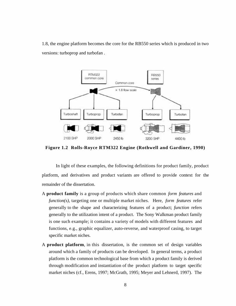
8
1.8, the engine platform becomes the core for the RB550 series which is produced in two
versions: turboprop and turbofan .
Figure 1.2 Rolls-Royce RTM322 Engine (Rothwell and Gardiner, 1990)
In light of these examples, the following definitions for product family, product
platform, and derivatives and product variants are offered to provide context for the
remainder of the dissertation.
A product family is a group of products which share common form features and
function(s), targeting one or multiple market niches. Here, form features refer
generally to the shape and characterizing features of a product; function refers
generally to the utilization intent of a product. The Sony Walkman product family
is one such example; it contains a variety of models with different features and
functions, e.g., graphic equalizer, auto-reverse, and waterproof casing, to target
specific market niches.
A product platform, in this dissertation, is the common set of design variables
around which a family of products can be developed. In general terms, a product
platform is the common technological base from which a product family is derived
through modification and instantiation of the product platform to target specific
market niches (cf., Erens, 1997; McGrath, 1995; Meyer and Lehnerd, 1997). The
9
universal motor platform developed by Black & Decker is an example of a
successful product platform. Product platforms are also prevalent in the automobile
industry, for example, where several car models are typically derivatives of a
common platform (cf., Siddique and Rosen, 1998); Kobe (1997) and Naughton
(1997) describe GM’s and Honda’s global platform strategies, respectively.
A derivative or product variant is a specific instantiation of a product platform
within a product family which possesses unique form features and function(s) from
other members in the product family. Paper copiers are good examples of products
derived from a common product platform; in addition to the Canon example
discussed previously, Xerox’s 1090 copier is a derivative of its 1075 model while
both copiers are part of Xerox’s 10 series of copiers (Jacobson and Hillkirk, 1986).
Furthermore, the Boeing 747-200, 747-300, and 747-400 are derivatives of the
Boeing 747 (Rothwell and Gardiner, 1990).
A single product or individual product is a unique product that has no pre-defined
relationships to other products; any resemblance to other products is strictly through
coincidence or producer’s preference (Erens, 1997). A single product contrasts a
derivative product that has similarities to other products in the product family
having been derived from the same product platform.
In light of these examples and definitions, opportunities for making contributions in
product family and product platform design are discussed in the next section.
1 .1 .2 Opportunities in Product Family Design and Product Platform Design
To understand some of the research opportunities in product family and product
platform design, a closer look at the previous examples is needed. The examples from
Lutron, Nippondenso, and Black & Decker exemplify an a posteriori or bottom-up
approach to product family design. Each company redesigned or consolidated a group of
distinct products to create a more “efficient and effective” product family. Here, efficient
and effective refers to the increased economies of scale each company was able to realize by
standardizing components to reduce manufacturing and inventory costs without
significantly compromising product quality and performance.
10
The main drivers for this type of approach are as follows:
• simplify the product offering and reduce part variety by
• standardizing components so as to
• reduce manufacturing costs and inventory costs and
• reduce manufacturing variability (i.e., the variety of parts that are produced in a
given manufacturing facility) and thereby
• improve quailty and customer satisfaction.
While the cost savings in manufacturing and inventory begin almost immediately from this
type of approach, the rewards are typically long-term since the capital investments and
redesign costs can be significant. Black & Decker, for example, estimated that it would
take seven years to reach the break-even point when they redesigned their universal motor
platform for Double Insulation. As Lehnerd (1987) discusses, between capital
expenditures, development, and tooling, Black & Decker spent $17M to redesign their
motors; however, by paying attention to standardization and exploiting platform scaling
around the motor stack length, all of their motors could be produced on the same machines.
As a result, material costs dropped from $0.77 to $0.42 per motor while labor costs fell
from $0.248 to $0.045 per motor, yielding an annual savings of $1.82M per year. The
cost of Black & Decker tools decreased by as much as 62%, boosting sales, increasing
production volumes, and further improving savings.
But must a company spend millions of dollars in costly redesign to achieve a good
product family? The answer is obviously no, and the examples from Rolls Royce, Canon,
and Sony demonstrate such an approach. These three companies exemplify an a priori or
top-down approach to product family design, i.e., strategically manage and develop a
family of products based on a common platform and its derivatives. McGrath (1995) states
that “A clear platform strategy leverages the resulting products, enabling them to be
11
deployed rapidly and consistently.” Furthermore, Wheelwright and Clark (1992) write as
follows:
“Companies target new platforms to meet the needs of a core group of customers
but design them for easy modification into derivatives through the addition,
substitution, or removal of features. Well-designed platforms also provide a
smooth migration path between generations so neither the customer nor the
distribution channel is disrupted.”
Finally, commonality and standardization across product families allow new designs to be
introduced, exploited, and retired with minimal expense related to product development
(Lehnerd, 1987).
As discussed in Section 1.1.1, Sony and Canon have been able to dominate their
respective markets despite serious local and global competition through a well managed
product platform implementation strategy. The Sony Walkman has been the leader in the
personal stereo market for decades; Sanderson and Uzumeri (1995) studied the success of
the Sony Walkman, commenting as follows:
“Sony's strategy employed a judicious mix of design projects, ranging from large
team efforts that produced major new model 'platforms' to minor tweaking of
existing designs. Throughout, Sony followed a disciplined and creative approach
to focus its sub-families on clear design goals and target models to distinct market
segments. Sony supported its design efforts with continuous innovation in features
and capabilities, as well as key investments in flexible manufacturing.”
Similiarly, Canon was able to steal, and henceforth dominate, the low-end copier market
from Xerox through careful development and realization of a family of products derived
from common platforms (Jacobson and Hillkirk, 1986). Companies like Xerox now are in
the process of re-engineering their product development processes to facilitate the design
and development of new families of copiers in record time (Paula, 1997). Along these
same lines, Rolls Royce can boast similar success. By scaling the RTM322 engine
platform to satisfy a range of thrust and power requirements, Rolls Royce was able to (a)
12
reduce manufacturing and inventory costs by using similar modules and components from
one engine to the next and, more importantly, (b) facilitate the costly certification phase of
its engine development process.
Good product platforms do not just come off the shelf; they must be carefully
planned, designed, and developed. This requires intimate knowledge of customer
requirements and a thorough understanding of the market. However, as discussed in the
literature review in Section 2.2.1, many of the tools and methods which have been
developed to facilitate the management and development of effective product platforms and
product families are at too high of a level of abstraction to be useful to engineering
designers particularly for modeling and design synthesis. Meanwhile, engineering design
methods and tools for synthesizing product families and product platforms are limited or
slowly evolving. Consider the brief summary in Table 1.1 of the product family examples
from Section 1.1.1 and the availability of design support. The majority of the examples
from Section 1.1.1 require modular design to facilitate upgrading and derating product
variants through the addition and removal of modules; a survey of these many of
approaches is offered in Section 2.2.3. In additioin, clustering approaches have been
developed to reduce variability within a product family and facilitate redesigning product
families to improve component commonality, see Section 2.2.3. Meanwhile, little to no
attention has been paid to platform scaling issues for product family design. The notion of
a “scalable” or “stretchable” product platform is introduced by Rothwell and Gardiner
(1990) and may be loosely defined as follows:
Scalable refers to the capability of a product platform to be “scaled,” “stretched,” or
“leveraged” to satisfy specific market niches. For example, the Boeing 747 is a
scalable product platform. It has been “scaled up” and “scaled down” to create the
Boeing 747-200, 747-300, and 747-400 to satisfy different market niches based on
number of passengers, flight range, etc. (Rothwell and Gardiner, 1990). The
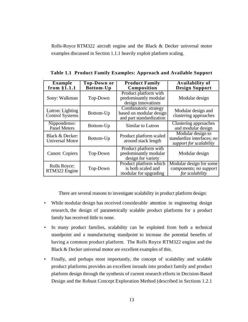
13
Rolls-Royce RTM322 aircraft engine and the Black & Decker universal motor
examples discussed in Section 1.1.1 heavily exploit platform scaling.
Table 1.1 Product Family Examples: Approach and Available Support
Examplefrom §1.1.1
Top-Down orBottom-Up
Product FamilyComposition
Availability ofDesign Support
Sony: Walkman Top-DownProduct platform withpredominantly modular
design innovationsModular design
Lutron: LightingControl Systems Bottom-Up
Combinatoric strategybased on modular designand part standardization
Modular design andclustering approaches
Nippondenso:Panel Meters Bottom-Up Similar to Lutron Clustering approaches
and modular design
Black & Decker:Universal Motor Bottom-Up Product platform scaled
around stack length
Modular design tostandardize interfaces; no
support for scalability
Canon: Copiers Top-DownProduct platform withpredominantly modular
design for varietyModular design
Rolls Royce:RTM322 Engine Top-Down
Product platform whichis both scaled and
modular for upgrading
Modular design for somecomponents; no support
for scalability
There are several reasons to investigate scalability in product platform design:
• While modular design has received considerable attention in engineering design
research, the design of parametrically scalable product platforms for a product
family has received little to none.
• In many product families, scalability can be exploited from both a technical
standpoint and a manufacturing standpoint to increase the potential benefits of
having a common product platform. The Rolls Royce RTM322 engine and the
Black & Decker universal motor are excellent examples of this.
• Finally, and perhaps most importantly, the concept of scalability and scalable
product platforms provides an excellent inroads into product family and product
platform design through the synthesis of current research efforts in Decision-Based
Design and the Robust Concept Exploration Method (described in Sections 1.2.1
14
and 1.2.2, respectively), robust design (described in Section 2.3) and tools from
marketing/management science (described in Section 2.2.1).
Consequently, the primary research question investigated in this dissertation is as follows:
How can a common scalable product platform be modeled and designed for a
product family?
To address this question, the Product Platform Concept Exploration Method
(PPCEM) is developed in this dissertation to provide a Method which facilitates the
synthesis and Exploration of a common Product Platform Concept which can be scaled into
an appropriate family of products. The PPCEM and its associated tools and steps are
introduced in Section 3.1. The underlying assumption behind the PPCEM is that a
common set of specifications (i.e., design variable settings) can be found for a product
platform which can then be scaled in one or more of its “dimensions” to realize a product
family. This product family can then satisfy a wide variety of customer requirements with
minimal compromise in individual product quality and performance even though the
product family is derived from a common platform through scaling. Although the PPCEM
is predominantly a method for parameteric or variant design, it is asserted that commonality
of product dimensions and specifications promotes commonality of components which
leads to reduced manufacturing and inventory costs through better economies of scale and
amortization of capital investment over a wider variety of derivative products based on the
common product platform. In special cases, such as the Rolls Royce RTM322 engine
platform mentioned earlier and the Boeing 747 series of aircraft, an added benefit of scaling
a common product platform is to expidite the testing and certification phase of development
(cf., Rothwell and Gardiner, 1990). The foundation for developing this approach is
15
presented in the next section. The specific research focus for the dissertation then is
outlined in Section 1.3.
1.2 FOUNDATIONS FOR DESIGNING SCALABLE PRODUCTPLATFORMS FOR A PRODUCT FAMILY
The technology base for the dissertation is described in this section. An overview
of Decision-Based Design, the design paradigm subscribed to in this dissertation, and the
compromise Decision Support Problem is given in Section 1.2.1. This is followed by an
overview of the Robust Concept Exploration Method (from which the Product Platform
Concept Exploration Method is derived) in Section 1.2.2.
1 .2 .1 Decision-Based Design, the Decision Support Problem Technique,and the Compromise Decision Support Problem
Decision-Based Design (DBD) is rooted in the notion that the principal role of a
designer in the design of an artifact is to make decisions (see, e.g., Muster and Mistree,
1988). This role is useful in providing a starting point for developing design methods
based on paradigms that spring from the perspective of decisions made by designers (who
may use computers) as opposed to design that is predicated on the use of computers,
optimization methods (computer-aided design optimization), or methods that evolve from
specific analysis tools such as finite element analysis.
The implementation of Decision-Based Design that is employed in this dissertation
is the Decision Support Problem (DSP) Technique (see, e.g., Bras and Mistree, 1991), a
technique that supports human judgment in designing systems that can be manufactured
and maintained. In the DSP Technique, designing is defined as the process of converting
information that characterizes the needs and requirements for a product into knowledge
about a product (Mistree, et al., 1990). This definition is extended easily to product family
design: the process of converting information that characterizes the needs and requirements
16
for a product family into knowledge about a product family, or as is the case of this work,
a common scalable product platform. A complete description of the DSP Technique can be
found in, e.g., (e.g., Mistree, et al., 1990).
Among the tools available within the DSP Technique, the compromise DSP
(Mistree, et al., 1993) is a general framework for solving multiobjective, non-linear,
optimization problems. In this dissertation, the compromise DSP is central to modeling
multiple design objectives and assessing the tradeoffs pertinent to product family and
product platform design. Examples of these tradeoffs are discussed in the context of the
two example problems in Chapters 6 and 7.
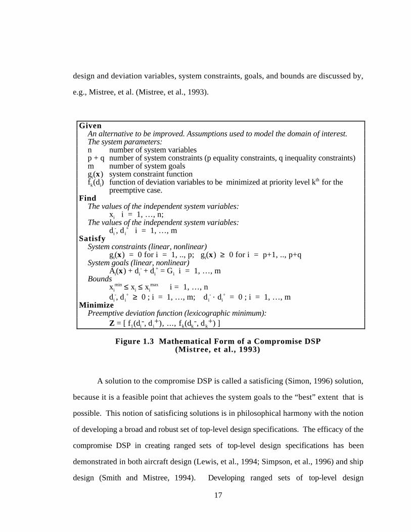
Mathematically, the compromise DSP is a multiobjective decision model which is a
hybrid formulation based on Mathematical Programming and Goal Programming (Mistree,
et al., 1993), see Figure 1.3. The compromise DSP is used to determine the values of the
design variables which satisfy a set of constraints and bounds and achieve as closely as
possible a set of conflicting goals. The compromise DSP is solved using the Adaptive
Linear Programming (ALP) algorithm which is based on sequential linear programming
and is part of the DSIDES (Decision Support in Designing Engineering Systems) software
(Mistree, et al., 1993).
In the compromise DSP, goals either may be weighted in an Archimedean solution
scheme or rank-ordered into priority levels using a preemptive approach to effect a solution
on the basis of preference. For the preemptive approach, the lexicographic minimum
concept (Ignizio, 1985) is used to evaluate different design scenarios quickly by changing
the priority levels of the goals to be achieved. The capabilities of the lexicographic
minimum concept are employed to develop the product platform portfolio as discussed in
Section 3.1.4, with further examples in Sections 6.4 and 7.5. Differences between the
Archimedean and preemptive deviation functions and a description of the ALP algorithm,
17
design and deviation variables, system constraints, goals, and bounds are discussed by,
e.g., Mistree, et al. (Mistree, et al., 1993).
GivenAn alternative to be improved. Assumptions used to model the domain of interest.The system parameters:n number of system variablesp + q number of system constraints (p equality constraints, q inequality constraints)m number of system goalsgi(x) system constraint functionfk(di) function of deviation variables to be minimized at priority level kth for the
preemptive case.Find
The values of the independent system variables:xi i = 1, …, n;
The values of the independent system variables:di
-, d i+ i = 1, …, m
SatisfySystem constraints (linear, nonlinear)
gi(x) = 0 for i = 1, .., p; gi(x) ≥ 0 for i = p+1, .., p+qSystem goals (linear, nonlinear)
Ai(x) + di- + di
+ = Gi i = 1, …, mBounds
ximin ≤ xi ≤ xi
max i = 1, …, ndi
-, d i+ ≥ 0 ; i = 1, …, m; d i
- . di+ = 0 ; i = 1, …, m
MinimizePreemptive deviation function (lexicographic minimum):
Z = [ f1(di-, d i
+), ..., fk(dk-, dk
+) ]
Figure 1.3 Mathematical Form of a Compromise DSP(Mistree, et al., 1993)
A solution to the compromise DSP is called a satisficing (Simon, 1996) solution,
because it is a feasible point that achieves the system goals to the “best” extent that is
possible. This notion of satisficing solutions is in philosophical harmony with the notion
of developing a broad and robust set of top-level design specifications. The efficacy of the
compromise DSP in creating ranged sets of top-level design specifications has been
demonstrated in both aircraft design (Lewis, et al., 1994; Simpson, et al., 1996) and ship
design (Smith and Mistree, 1994). Developing ranged sets of top-level design
18
specifications is generalized into the notion of developing a product platform portfolio
which is discussed in Section 3.1.5. By finding a “portfolio” of solutions rather than a
single point solution, greater design flexibility can be maintained during the design process.
Finally, the compromise DSP also provides the cornerstone of the Robust Concept
Exploration Method which is reviewed in the next section.
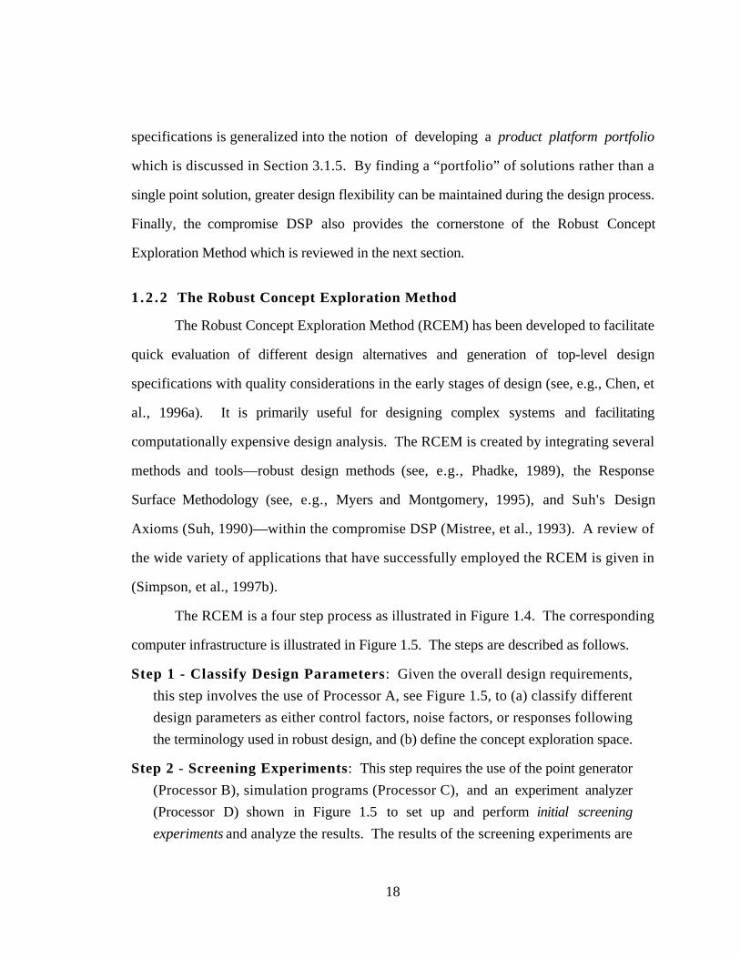
1 .2 .2 The Robust Concept Exploration Method
The Robust Concept Exploration Method (RCEM) has been developed to facilitate
quick evaluation of different design alternatives and generation of top-level design
specifications with quality considerations in the early stages of design (see, e.g., Chen, et
al., 1996a). It is primarily useful for designing complex systems and facilitating
computationally expensive design analysis. The RCEM is created by integrating several
methods and tools—robust design methods (see, e.g., Phadke, 1989), the Response
Surface Methodology (see, e.g., Myers and Montgomery, 1995), and Suh's Design
Axioms (Suh, 1990)—within the compromise DSP (Mistree, et al., 1993). A review of
the wide variety of applications that have successfully employed the RCEM is given in
(Simpson, et al., 1997b).
The RCEM is a four step process as illustrated in Figure 1.4. The corresponding
computer infrastructure is illustrated in Figure 1.5. The steps are described as follows.
Step 1 - Classify Design Parameters: Given the overall design requirements,
this step involves the use of Processor A, see Figure 1.5, to (a) classify different
design parameters as either control factors, noise factors, or responses following
the terminology used in robust design, and (b) define the concept exploration space.
Step 2 - Screening Experiments: This step requires the use of the point generator
(Processor B), simulation programs (Processor C), and an experiment analyzer
(Processor D) shown in Figure 1.5 to set up and perform initial screening
experiments and analyze the results. The results of the screening experiments are
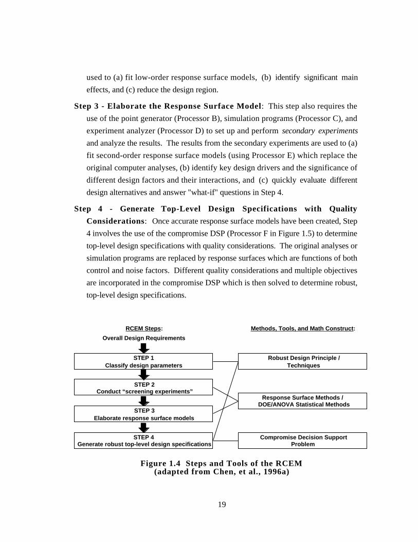
19
used to (a) fit low-order response surface models, (b) identify significant main
effects, and (c) reduce the design region.
Step 3 - Elaborate the Response Surface Model: This step also requires the
use of the point generator (Processor B), simulation programs (Processor C), and
experiment analyzer (Processor D) to set up and perform secondary experiments
and analyze the results. The results from the secondary experiments are used to (a)
fit second-order response surface models (using Processor E) which replace the
original computer analyses, (b) identify key design drivers and the significance of
different design factors and their interactions, and (c) quickly evaluate different
design alternatives and answer "what-if" questions in Step 4.
Step 4 - Generate Top-Level Design Specifications with Quality
Considerations: Once accurate response surface models have been created, Step
4 involves the use of the compromise DSP (Processor F in Figure 1.5) to determine
top-level design specifications with quality considerations. The original analyses or
simulation programs are replaced by response surfaces which are functions of both
control and noise factors. Different quality considerations and multiple objectives
are incorporated in the compromise DSP which is then solved to determine robust,
top-level design specifications.
STEP 4Generate robust top-level design specifications
Overall Design Requirements
RCEM Steps: Methods, Tools, and Math Construct:
STEP 3Elaborate response surface models
STEP 2Conduct “screening experiments”
STEP 1Classify design parameters
Robust Design Principle /Techniques
Response Surface Methods / DOE/ANOVA Statistical Methods
Compromise Decision SupportProblem
Figure 1.4 Steps and Tools of the RCEM(adapted from Chen, et al., 1996a)
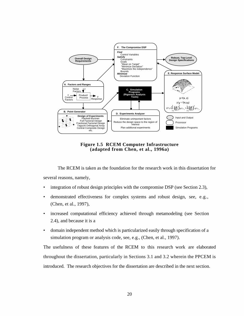
20
Robust, Top-LevelDesign Specifications
E. Response Surface Model
y=f(x, z)
µˆy = f(x,µz)
σ2ˆy=Σi=1
k∂f∂zi( )
2
σ2ˆz ii=1
l∂f∂xi( )
2
σ2ˆx i+Σ
Input and Output
Processor
Simulation Programs
D. Experiments Analyzer
Eliminate unimportant factorsReduce the design space to the region of
interestPlan additional experiments
Overall Design Requirements
A. Factors and Ranges
Product/ Process
Noise zFactors
yResponse
xControlFactors
B. Point Generator
Design of ExperimentsPlackett-Burman
Full Factorial DesignFractional Factorial DesignTaguchi Orthogonal ArrayCentral Composite Design
etc.
C. Simulation Programs
(Rigorous Analysis Tools)
F. The Compromise DSP
Find Control VariablesSatisfy Constraints Goals "Mean on Target" "Minimize Deviation" “Maximize the independence” BoundsMinimize Deviation Function
Figure 1.5 RCEM Computer Infrastructure(adapted from Chen, et al., 1996a)
The RCEM is taken as the foundation for the research work in this dissertation for
several reasons, namely,
• integration of robust design principles with the compromise DSP (see Section 2.3),
• demonstrated effectiveness for complex systems and robust design, see, e.g.,
(Chen, et al., 1997),
• increased computational efficiency achieved through metamodeling (see Section
2.4), and because it is a
• domain independent method which is particularized easily through specification of a
simulation program or analysis code, see, e.g., (Chen, et al., 1997).
The usefulness of these features of the RCEM to this research work are elaborated
throughout the dissertation, particularly in Sections 3.1 and 3.2 wherein the PPCEM is
introduced. The research objectives for the dissertation are described in the next section.
21
1.3 RESEARCH FOCUS IN THE DISSERTATION
The research focus in this dissertation is embodied as follows:
• a set of research questions that capture motivation and specific issues to be
addressed,
• a set of corresponding research hypotheses that offer a context by which the
research proceeds, defining the structure of the verification studies performed in
this work, and
• a set of resulting research contributions that embody the deliverables from the
research in terms of intellectual value, a repeatable method of solution, limitations,
and avenues of further investigation.
The research questions are presented in Section 1.3.1 along with the corresponding
research hypotheses. The research hypotheses (and supporting posits) are discussed in
more detail in Section 3.2 along with issues of verification and validation. The resulting
research contributions are introduced in Section 1.3.2.
1 .3 .1 Research Questions and Hypotheses in the Dissertation
The principal goal in this dissertation is the development of a method to facilitate the
design of a scalable product platform around which a family of products can be developed.
As discussed in the previous section, Decision-Based Design and the RCEM provide the
foundation on which this work is built. Given this foundation and goal, the motivation for
this research is embodied in the primary research question identified in Section 1.1.2 which
is repeated here.
Primary Research Question:
Q1. How can a common scalable product platform be modeled and designed for a
product family?
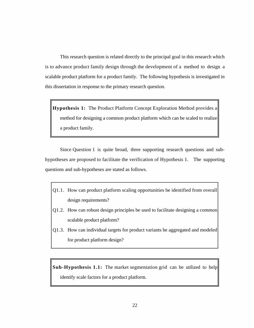
22
This research question is related directly to the principal goal in this research which
is to advance product family design through the development of a method to design a
scalable product platform for a product family. The following hypothesis is investigated in
this dissertation in response to the primary research question.
Hypothesis 1: The Product Platform Concept Exploration Method provides a
method for designing a common product platform which can be scaled to realize
a product family.
Since Question 1 is quite broad, three supporting research questions and sub-
hypotheses are proposed to facilitate the verification of Hypothesis 1. The supporting
questions and sub-hypotheses are stated as follows.
Q1.1. How can product platform scaling opportunities be identified from overall
design requirements?
Q1.2. How can robust design principles be used to facilitate designing a common
scalable product platform?
Q1.3. How can individual targets for product variants be aggregated and modeled
for product platform design?
Sub-Hypothesis 1.1: The market segmentation grid can be utilized to help
identify scale factors for a product platform.
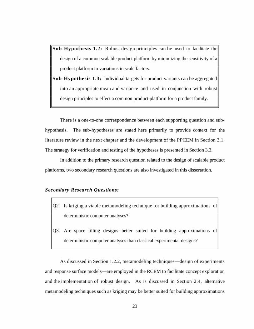
23
Sub-Hypothesis 1.2: Robust design principles can be used to facilitate the
design of a common scalable product platform by minimizing the sensitivity of a
product platform to variations in scale factors.
Sub-Hypothesis 1.3: Individual targets for product variants can be aggregated
into an appropriate mean and variance and used in conjunction with robust
design principles to effect a common product platform for a product family.
There is a one-to-one correspondence between each supporting question and sub-
hypothesis. The sub-hypotheses are stated here primarily to provide context for the
literature review in the next chapter and the development of the PPCEM in Section 3.1.
The strategy for verification and testing of the hypotheses is presented in Section 3.3.
In addition to the primary research question related to the design of scalable product
platforms, two secondary research questions are also investigated in this dissertation.
Secondary Research Questions:
Q2. Is kriging a viable metamodeling technique for building approximations of
deterministic computer analyses?
Q3. Are space filling designs better suited for building approximations of
deterministic computer analyses than classical experimental designs?
As discussed in Section 1.2.2, metamodeling techniques—design of experiments
and response surface models—are employed in the RCEM to facilitate concept exploration
and the implementation of robust design. As is discussed in Section 2.4, alternative
metamodeling techniques such as kriging may be better suited for building approximations
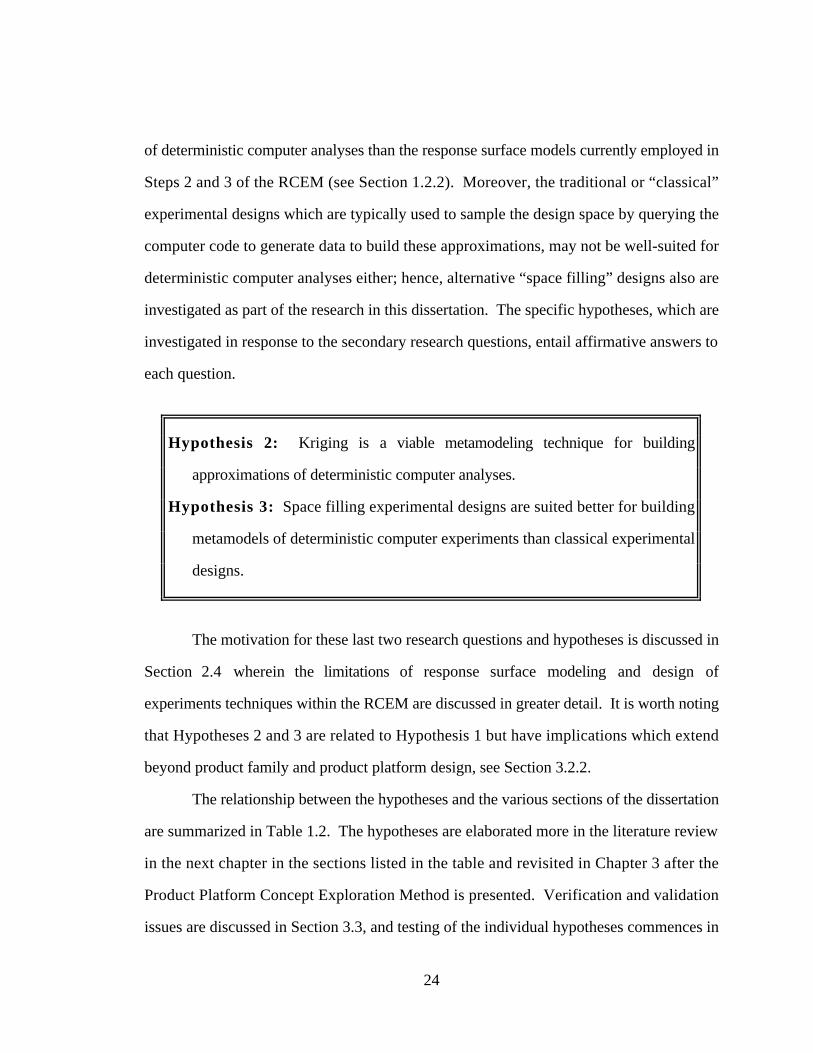
24
of deterministic computer analyses than the response surface models currently employed in
Steps 2 and 3 of the RCEM (see Section 1.2.2). Moreover, the traditional or “classical”
experimental designs which are typically used to sample the design space by querying the
computer code to generate data to build these approximations, may not be well-suited for
deterministic computer analyses either; hence, alternative “space filling” designs also are
investigated as part of the research in this dissertation. The specific hypotheses, which are
investigated in response to the secondary research questions, entail affirmative answers to
each question.
Hypothesis 2: Kriging is a viable metamodeling technique for building
approximations of deterministic computer analyses.
Hypothesis 3: Space filling experimental designs are suited better for building
metamodels of deterministic computer experiments than classical experimental
designs.
The motivation for these last two research questions and hypotheses is discussed in
Section 2.4 wherein the limitations of response surface modeling and design of
experiments techniques within the RCEM are discussed in greater detail. It is worth noting
that Hypotheses 2 and 3 are related to Hypothesis 1 but have implications which extend
beyond product family and product platform design, see Section 3.2.2.
The relationship between the hypotheses and the various sections of the dissertation
are summarized in Table 1.2. The hypotheses are elaborated more in the literature review
in the next chapter in the sections listed in the table and revisited in Chapter 3 after the
Product Platform Concept Exploration Method is presented. Verification and validation
issues are discussed in Section 3.3, and testing of the individual hypotheses commences in
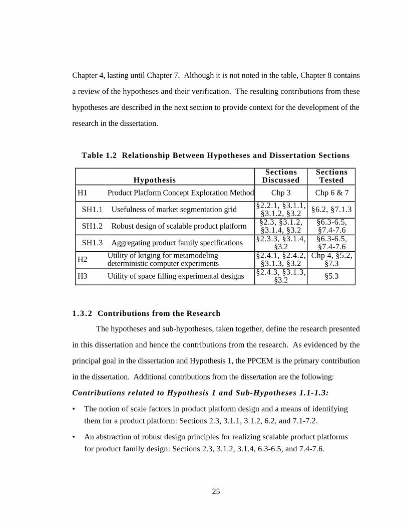
25
Chapter 4, lasting until Chapter 7. Although it is not noted in the table, Chapter 8 contains
a review of the hypotheses and their verification. The resulting contributions from these
hypotheses are described in the next section to provide context for the development of the
research in the dissertation.
Table 1.2 Relationship Between Hypotheses and Dissertation Sections
HypothesisSections
DiscussedSectionsTested
H1 Product Platform Concept Exploration Method Chp 3 Chp 6 & 7
SH1.1 Usefulness of market segmentation grid §2.2.1, §3.1.1,§3.1.2, §3.2 §6.2, §7.1.3
SH1.2 Robust design of scalable product platform §2.3, §3.1.2,§3.1.4, §3.2
§6.3-6.5,§7.4-7.6
SH1.3 Aggregating product family specifications §2.3.3, §3.1.4,§3.2
§6.3-6.5,§7.4-7.6
H2 Utility of kriging for metamodelingdeterministic computer experiments
§2.4.1, §2.4.2,§3.1.3, §3.2
Chp 4, §5.2,§7.3
H3 Utility of space filling experimental designs §2.4.3, §3.1.3,§3.2 §5.3
1 .3 .2 Contributions from the Research
The hypotheses and sub-hypotheses, taken together, define the research presented
in this dissertation and hence the contributions from the research. As evidenced by the
principal goal in the dissertation and Hypothesis 1, the PPCEM is the primary contribution
in the dissertation. Additional contributions from the dissertation are the following:
Contributions related to Hypothesis 1 and Sub-Hypotheses 1.1-1.3:
• The notion of scale factors in product platform design and a means of identifying
them for a product platform: Sections 2.3, 3.1.1, 3.1.2, 6.2, and 7.1-7.2.
• An abstraction of robust design principles for realizing scalable product platforms
for product family design: Sections 2.3, 3.1.2, 3.1.4, 6.3-6.5, and 7.4-7.6.
26
• Non-commonality and performance deviation measures for performing product
variety tradeoff studies, see Sections 3.1.5 and 7.6.2.
Contributions related to Hypothesis 2:
• An algorithm to build, validate, and use a kriging model: Section 2.4.2, Chapters 4,
5, and 7, and Appendix A.
• A preliminary comparison of the predictive capability of second-order response
surface models and kriging models: Chapter 4.
• An investigation of the effect of five different spatial correlation functions on the
accuracy of a kriging model: Section 2.4.2 and Chapter 5.
Contributions related to Hypothesis 3:
• An investigation of the effect of eleven different experimental designs on building
an accurate kriging model: Section 2.4.3 and Chapter 5.
• An algorithm for generating minimax Latin hypercube designs: Section 2.4.3 and
Appendix C.
This being the first chapter of the dissertation, these contributions cannot be substantiated;
therefore, they are revisited in Section 8.1 after all of the research findings have been
documented and discussed. An overview of the dissertation is presented next.
1.4 OVERVIEW OF THE DISSERTATION
To facilitate this discussion, an overview of the chapters in the dissertation is
shown in Figure 1.6. Having lain the foundation by introducing the research questions and
hypotheses for the work in this chapter, the next chapter contains a literature review of
related research, elucidating the problems and opportunities in product family and product
platform design. Three research areas are reviewed: (1) product family and product
platform design with particular emphasis on scalability and sizing, (2) robust design and its
application in engineering design, and (3) statistical metamodeling and its role in
27
engineering design, see Sections 2.2, 2.3, and 2.4, respectively. A discussion of how
these disparate research areas relate to one another is offered in Section 2.1
The PPCEM is introduced in Chapter 3 as elements from Chapters 1 and 2 are
synthesized into a method for designing a scalable product platform for a product family.
The PPCEM and its associated steps are presented in Section 3.1. After the PPCEM is
presented, the research hypotheses are revisited in Section 3.2, and supporting posits are
stated and substantiated. Section 3.3 contains an outline of the strategy for verification and
testing of the hypotheses which includes a preview of Chapters 4 and 5—wherein
Hypotheses 2 and 3 are tested—and Chapters 6 and 7 wherein the PPCEM is applied to
two example problems, verifying Hypotheses 1 and Sub-Hypotheses 1.1 through 1.3.
Testing of the hypotheses begins in Chapter 4, but Chapters 4 and 5 entail a brief
departure from product platform design yet are an integral part of the development of the
PPCEM. In Chapter 4, an initial feasibility study of the usefulness of kriging is performed
to familiarize the reader with the method and to begin to verify Hypotheses 2 by comparing
the accuracy of kriging models to second-order response surface models, the current
standard in metamodeling. In Chapter 5, an extensive study of six engineering test
problems selected from the literature is conducted to determine the utility of kriging
metamodels and various experimental designs, testing and verifying Hypotheses 2 and 3.
Once the kriging/DOE study is completed in Chapter 5, the first of two examples
used to demonstrate the PPCEM and verify its associated hypotheses is given in Chapter 6:
the design of a family of universal electric motors. This first example employs the PPCEM
without any metamodeling, providing “proof of concept” that the method works. Then, in
Chapter 7 the PPCEM is applied to the design of a family of General Aviation aircraft,
making full use of the kriging metamodels and robust design capabilities. In each chapter,
an overview of the problem is given along with pertinent analysis information, the steps of
the PPCEM are performed, and the ramifications of the results are discussed.
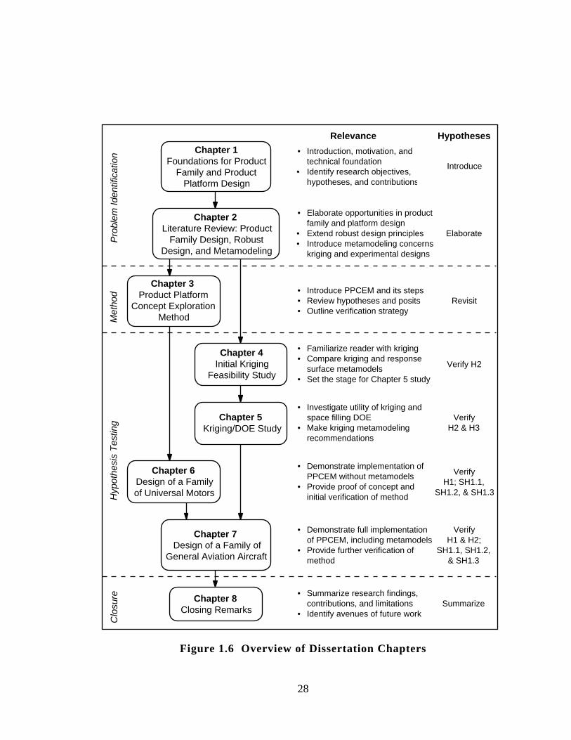
28
• Introduction, motivation, andtechnical foundation
• Identify research objectives, hypotheses, and contributions
Relevance
• Elaborate opportunities in productfamily and platform design
• Extend robust design principles• Introduce metamodeling concerns:
kriging and experimental designs
• Introduce PPCEM and its steps• Review hypotheses and posits• Outline verification strategy
• Familiarize reader with kriging• Compare kriging and response
surface metamodels• Set the stage for Chapter 5 study
• Investigate utility of kriging and space filling DOE
• Make kriging metamodelingrecommendations
• Demonstrate implementation of PPCEM without metamodels
• Provide proof of concept and initial verification of method
• Demonstrate full implementationof PPCEM, including metamodels
• Provide further verification ofmethod
• Summarize research findings,contributions, and limitations
• Identify avenues of future work
Chapter 3 Product Platform
Concept Exploration Method
Chapter 4Initial Kriging
Feasibility Study
Chapter 5 Kriging/DOE Study
Chapter 6 Design of a Family of Universal Motors
Chapter 7 Design of a Family of
General Aviation Aircraft
Chapter 8 Closing Remarks
Chapter 2 Literature Review: Product
Family Design, Robust Design, and Metamodeling
Chapter 1Foundations for Product
Family and Product Platform Design
Pro
ble
m I
dentif
icatio
nM
eth
od
Hyp
oth
esi
s T
est
ing
Hypotheses
Verify H2
VerifyH2 & H3
VerifyH1; SH1.1,
SH1.2, & SH1.3
VerifyH1 & H2;
SH1.1, SH1.2, & SH1.3
Clo
sure
Revisit
Elaborate
Introduce
Summarize
Figure 1.6 Overview of Dissertation Chapters
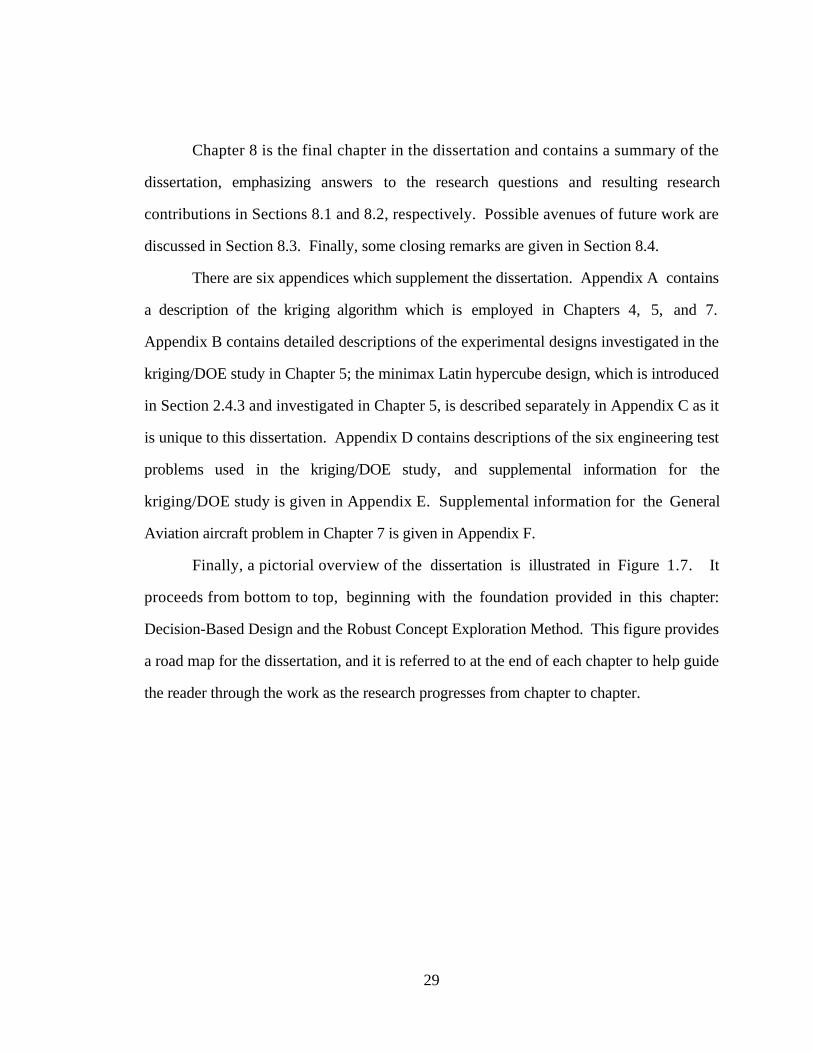
29
Chapter 8 is the final chapter in the dissertation and contains a summary of the
dissertation, emphasizing answers to the research questions and resulting research
contributions in Sections 8.1 and 8.2, respectively. Possible avenues of future work are
discussed in Section 8.3. Finally, some closing remarks are given in Section 8.4.
There are six appendices which supplement the dissertation. Appendix A contains
a description of the kriging algorithm which is employed in Chapters 4, 5, and 7.
Appendix B contains detailed descriptions of the experimental designs investigated in the
kriging/DOE study in Chapter 5; the minimax Latin hypercube design, which is introduced
in Section 2.4.3 and investigated in Chapter 5, is described separately in Appendix C as it
is unique to this dissertation. Appendix D contains descriptions of the six engineering test
problems used in the kriging/DOE study, and supplemental information for the
kriging/DOE study is given in Appendix E. Supplemental information for the General
Aviation aircraft problem in Chapter 7 is given in Appendix F.
Finally, a pictorial overview of the dissertation is illustrated in Figure 1.7. It
proceeds from bottom to top, beginning with the foundation provided in this chapter:
Decision-Based Design and the Robust Concept Exploration Method. This figure provides
a road map for the dissertation, and it is referred to at the end of each chapter to help guide
the reader through the work as the research progresses from chapter to chapter.
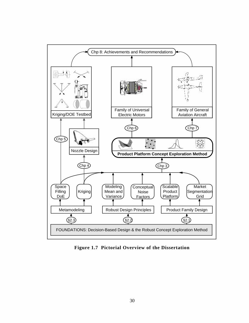
30
Nozzle Design
Chp 8: Achievements and Recommendations
Family of General Aviation AircraftKriging/DOE Testbed
Family of UniversalElectric Motors
Metamodeling
ModelingMean andVariance
Robust Design Principles
ConceptualNoise
Factors
ScalableProductPlatform
MarketSegmentation
Grid
Product Family Design
KrigingSpaceFillingDoE
Chp 6
Chp 4 Chp 3
§2.2§2.3 §2.1
Chp 5
Chp 7
FOUNDATIONS: Decision-Based Design & the Robust Concept Exploration Method
Platform
Product Platform Concept Exploration Method
Figure 1.7 Pictorial Overview of the Dissertation
31
2. CHAPTER 2
A LITERATURE REVIEW: PRODUCT FAMILYAND PRODUCT PLATFORM DESIGN, ROBUST
DESIGN, AND METAMODELING
Given the research focus identified in Section 1.3, a survey of relevant work in
product family and product platform design, robust design, and metamodeling is presented
in this chapter in Sections 2.2, 2.3, and 2.4, respectively. A thorough description of what
is in this chapter and how these disparate fields of research relate to each other is offered in
Section 2.1. In Section 2.2, the tools and methods for designing product families and
product platforms introduced in Section 1.1.2 are discussed in more detail. Section 2.3
then contains a review of robust design principles, focusing on robust design opportunities
in product family and product platform design. This segues into a discussion of
metamodeling and approximation techniques in Section 2.4 to facilitate the implementation
of robust design. In particular, the kriging approach to metamodeling is introduced in
Section 2.4.2 as a viable alternative for building approximations of deterministic computer
experiments, and a variety of space filling experimental designs for querying a computer
code to build kriging models are described in Section 2.4.3. Section 2.5 concludes the
chapter with a summary of what has been presented and a preview of what is next.
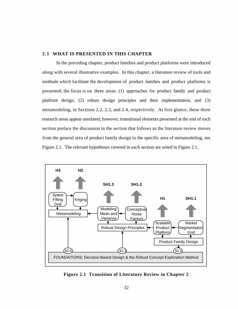
32
2.1 WHAT IS PRESENTED IN THIS CHAPTER
In the preceding chapter, product families and product platforms were introduced
along with several illustrative examples. In this chapter, a literature review of tools and
methods which facilitate the development of product families and product platforms is
presented; the focus is on three areas: (1) approaches for product family and product
platform design, (2) robust design principles and their implementation, and (3)
metamodeling, in Sections 2.2, 2.3, and 2.4, respectively. At first glance, these three
research areas appear unrelated; however, transitional elements presented at the end of each
section preface the discussion in the section that follows as the literature review moves
from the general area of product family design to the specific area of metamodeling, see
Figure 2.1. The relevant hypotheses covered in each section are noted in Figure 2.1.
SpaceFillingDoE
Metamodeling
Robust Design Principles
Product Family Design
FOUNDATIONS: Decision-Based Design & the Robust Concept Exploration Method
Kriging
ModelingMean andVariance
ConceptualNoise
FactorsScalableProductPlatform
MarketSegmentation
Grid
§2.3§2.4 §2.2
SH1.1H1
SH1.2SH1.3
H2H3
Figure 2.1 Transition of Literature Review in Chapter 2
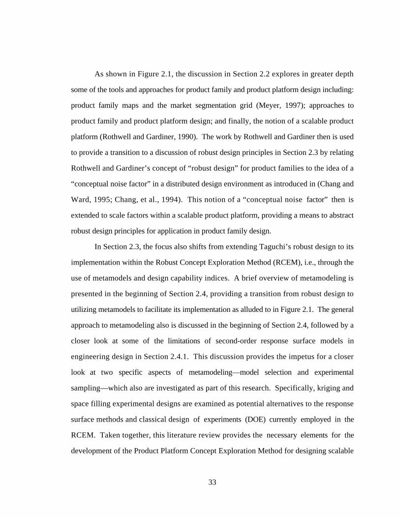
33
As shown in Figure 2.1, the discussion in Section 2.2 explores in greater depth
some of the tools and approaches for product family and product platform design including:
product family maps and the market segmentation grid (Meyer, 1997); approaches to
product family and product platform design; and finally, the notion of a scalable product
platform (Rothwell and Gardiner, 1990). The work by Rothwell and Gardiner then is used
to provide a transition to a discussion of robust design principles in Section 2.3 by relating
Rothwell and Gardiner’s concept of “robust design” for product families to the idea of a
“conceptual noise factor” in a distributed design environment as introduced in (Chang and
Ward, 1995; Chang, et al., 1994). This notion of a “conceptual noise factor” then is
extended to scale factors within a scalable product platform, providing a means to abstract
robust design principles for application in product family design.
In Section 2.3, the focus also shifts from extending Taguchi’s robust design to its
implementation within the Robust Concept Exploration Method (RCEM), i.e., through the
use of metamodels and design capability indices. A brief overview of metamodeling is
presented in the beginning of Section 2.4, providing a transition from robust design to
utilizing metamodels to facilitate its implementation as alluded to in Figure 2.1. The general
approach to metamodeling also is discussed in the beginning of Section 2.4, followed by a
closer look at some of the limitations of second-order response surface models in
engineering design in Section 2.4.1. This discussion provides the impetus for a closer
look at two specific aspects of metamodeling—model selection and experimental
sampling—which also are investigated as part of this research. Specifically, kriging and
space filling experimental designs are examined as potential alternatives to the response
surface methods and classical design of experiments (DOE) currently employed in the
RCEM. Taken together, this literature review provides the necessary elements for the
development of the Product Platform Concept Exploration Method for designing scalable

34
product platforms for a product family as presented in Chapter 3. Toward this end, the
state-of-art in product family and product platform design is discussed in the next section.
2.2 PRODUCT FAMILY AND PRODUCT PLATFORM DESIGN TOOLSAND METHODS
As stated in Section 1.1, in order to provide as much variety as possible for the
market with as little variety as possible between products, many researchers advocate a
product platform and product family approach to satisfy effectively a wide range of
customer needs. In Section 2.2.1, several attention directing tools developed to facilitate
product family and product platform design are presented. In Section 2.2.2, metrics for
assessing product platform effectiveness are discussed. Finally, in Section 2.2.3, methods
for product family design are reviewed.
2 .2 .1 Attention Directing Tools for Product Family and Product PlatformDesign
A large portion of the work in strategic marketing and management is focused on
either categorizing or mapping the evolution and development of product families. These
maps typically are applied a posteriori to a product family but can be used a priori to
identify new directions for product development within the product family. Examples of
product family maps include the work by Meyer and Utterback (1993) and Wheelwright
and Sasser (1989); a brief description of each follows.
Meyer and Utterback (1993) use the Product Family Map shown in Figure 2.2 to
trace the evolution of a product family. In their map, each generation of the product family
employs a platform as the foundation for targeting specific products at different (or
complimentary) markets. Improved designs and new technologies spawn successive
generations, and cost reductions and the addition and removal of features can lead to new
products. Multiple generations can be planned from existing ones, expanding to different
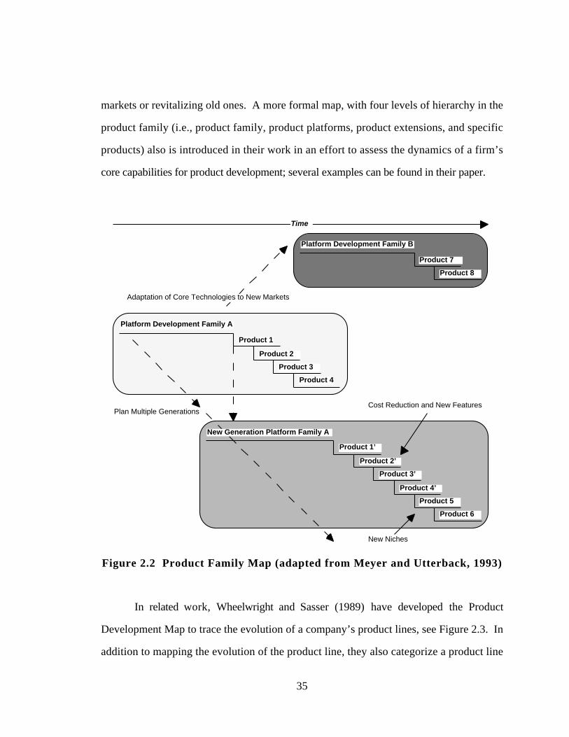
35
markets or revitalizing old ones. A more formal map, with four levels of hierarchy in the
product family (i.e., product family, product platforms, product extensions, and specific
products) also is introduced in their work in an effort to assess the dynamics of a firm’s
core capabilities for product development; several examples can be found in their paper.
Platform Development Family A
Product 1
Product 2
Product 3
Product 4
Product 7
Product 8
Product 5
Product 6
Product 1’
Product 2’
Product 3’
Product 4’
Platform Development Family B
Plan Multiple GenerationsCost Reduction and New Features
New Niches
Time
Adaptation of Core Technologies to New Markets
New Generation Platform Family A
Figure 2.2 Product Family Map (adapted from Meyer and Utterback, 1993)
In related work, Wheelwright and Sasser (1989) have developed the Product
Development Map to trace the evolution of a company’s product lines, see Figure 2.3. In
addition to mapping the evolution of the product line, they also categorize a product line
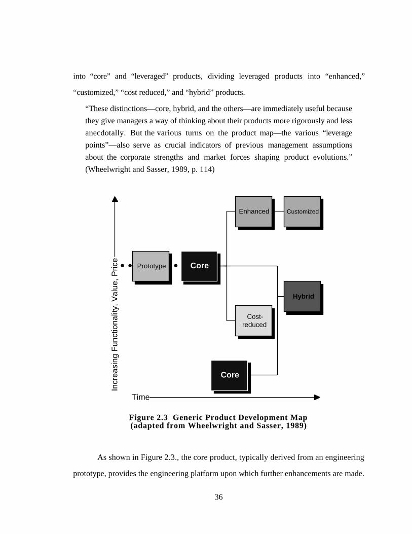
36
into “core” and “leveraged” products, dividing leveraged products into “enhanced,”
“customized,” “cost reduced,” and “hybrid” products.
“These distinctions—core, hybrid, and the others—are immediately useful because
they give managers a way of thinking about their products more rigorously and less
anecdotally. But the various turns on the product map—the various “leverage
points”—also serve as crucial indicators of previous management assumptions
about the corporate strengths and market forces shaping product evolutions.”
(Wheelwright and Sasser, 1989, p. 114)
Enhanced
Cost-reduced
Customized
Hybrid
• • • • • • • • •Prototype
Time
Core
Core
Incr
easi
ng F
unct
iona
lity,
Val
ue, P
rice
Figure 2.3 Generic Product Development Map(adapted from Wheelwright and Sasser, 1989)
As shown in Figure 2.3., the core product, typically derived from an engineering
prototype, provides the engineering platform upon which further enhancements are made.
37
Enhanced products are developed from the core by adding distinctive features to target
specific market niches; enhanced products are typically the first products leveraged from the
core product. Enhanced products can be customized further to provide more choice if
necessary. Cost-reduced products are “scaled” or “stripped” down versions (e.g., less
expensive materials and fewer features) of the core which are targeted at price-sensitive
markets. Finally the hybrid product is an entirely new design, resulting from the
combination of characteristics of two or more core products. As an example, the evolution
of three generations of a family of vacuum cleaners is mapped and discussed in their article.
These product family maps are useful attention directing tools for product family
design and development but offer little direction for designing a scalable product platform.
Toward this end, the market segmentation grid developed by Meyer (1997) facilitates
identifying leveraging strategies for a product platform, see Figure 2.4.
What Market NichesWill Your Product Platforms Serve?
High CostHigh Performance
Mid-Range
Low CostLow Performance
Segment A Segment B Segment C
Product Platform
Derivative Products
Figure 2.4 Product Platform Market Segmentation Grid(adapted from Meyer, 1997)

38
In a market segmentation grid, the major market segments serviced by a company’s
products are listed horizontally in the grid. The vertical axis reflects different tiers of price
and performance within each market segment. Several example instantiations of this grid
can be found in (Meyer, 1997; Meyer and Lehnerd, 1997) for companies such as Hewlett
Packard, Compaq, Steelcase, and Herman Miller.
This simple market segmentation grid can be used by firms to segment their
markets, helping to define a clear product platform strategy. For instance, a marketing
strategy which employs no leveraging is shown in Figure 2.5a. Companies which fail to
maintain a good platform leveraging strategy often have too many products that share too
little technology, resulting in a myriad of products, higher costs, and lower margins.
Three types of platform leveraging strategies can be identified within the market
segmentation grid: horizontal leveraging, vertical leveraging, and a beachhead approach as
shown in Figure 2.5b-d. All three leveraging strategies enable a more efficient and
effective product family to be developed. Examples of these leveraging strategies include
the following (Meyer, 1997):
Horizontally leveraging - subsystems of components within a product family are
leveraged from one market segment to the next within a given price/performance
tier. The main benefit of a horizontal leveraging strategy is to facilitate the
introduction of new products across a series of related market niches without
having to “reinvent the wheel.” Black & Decker often employs such a strategy:
“We don’t need to reinvent the power tool in every country, but rather, we have a
common product and adapt it to individual markets” states one of their top
executives (DiCamillo, 1988). Another example given by Meyer and his coauthors
is the Gillette Sensor-Excel razor which uses exactly the same razor cartridge in the
male and female market segments while the shape, color, and general design of the
handles are completely different for men’s and women’s.
Vertically leveraging - a product platform is leveraged to address a range of
price/performance tiers within a specific market segment. A company which excels
in the high-end segment of its market may scale down its platform into lower
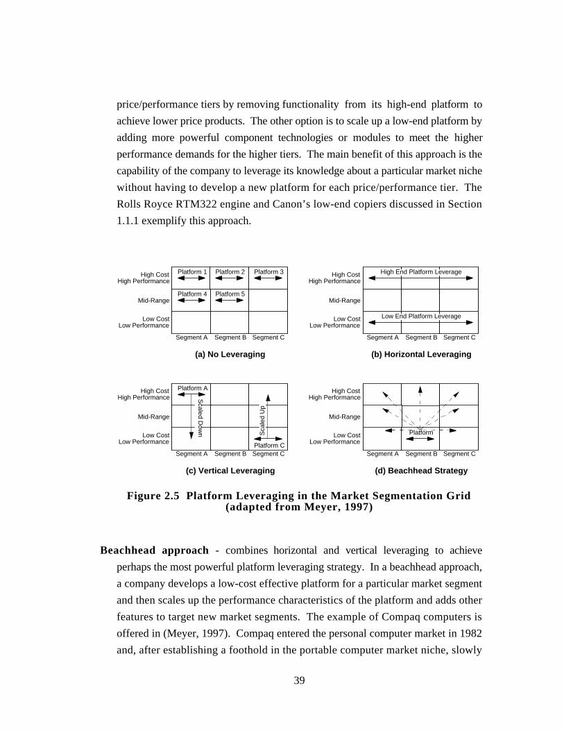
39
price/performance tiers by removing functionality from its high-end platform to
achieve lower price products. The other option is to scale up a low-end platform by
adding more powerful component technologies or modules to meet the higher
performance demands for the higher tiers. The main benefit of this approach is the
capability of the company to leverage its knowledge about a particular market niche
without having to develop a new platform for each price/performance tier. The
Rolls Royce RTM322 engine and Canon’s low-end copiers discussed in Section
1.1.1 exemplify this approach.
High CostHigh Performance
Mid-Range
Low CostLow Performance
Segment A Segment B Segment C
High CostHigh Performance
Mid-Range
Low CostLow Performance
Segment A Segment B Segment C
High CostHigh Performance
Mid-Range
Low CostLow Performance
Segment A Segment B Segment C
High CostHigh Performance
Mid-Range
Low CostLow Performance
Platform 1 Platform 2 Platform 3
Platform 5Platform 4
Segment A Segment B Segment C
Platform A
Platform C
Scaled D
own S
cale
d U
p
High End Platform Leverage
Low End Platform Leverage
Platform
(a) No Leveraging (b) Horizontal Leveraging
(c) Vertical Leveraging (d) Beachhead Strategy
Figure 2.5 Platform Leveraging in the Market Segmentation Grid(adapted from Meyer, 1997)
Beachhead approach - combines horizontal and vertical leveraging to achieve
perhaps the most powerful platform leveraging strategy. In a beachhead approach,
a company develops a low-cost effective platform for a particular market segment
and then scales up the performance characteristics of the platform and adds other
features to target new market segments. The example of Compaq computers is
offered in (Meyer, 1997). Compaq entered the personal computer market in 1982
and, after establishing a foothold in the portable computer market niche, slowly
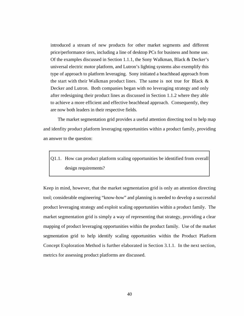
40
introduced a stream of new products for other market segments and different
price/performance tiers, including a line of desktop PCs for business and home use.
Of the examples discussed in Section 1.1.1, the Sony Walkman, Black & Decker’s
universal electric motor platform, and Lutron’s lighting systems also exemplify this
type of approach to platform leveraging. Sony initiated a beachhead approach from
the start with their Walkman product lines. The same is not true for Black &
Decker and Lutron. Both companies began with no leveraging strategy and only
after redesigning their product lines as discussed in Section 1.1.2 where they able
to achieve a more efficient and effective beachhead approach. Consequently, they
are now both leaders in their respective fields.
The market segmentation grid provides a useful attention directing tool to help map
and idenfity product platform leveraging opportunities within a product family, providing
an answer to the question:
Q1.1. How can product platform scaling opportunities be identified from overall
design requirements?
Keep in mind, however, that the market segmentation grid is only an attention directing
tool; considerable engineering “know-how” and planning is needed to develop a successful
product leveraging strategy and exploit scaling opportunities within a product family. The
market segmentation grid is simply a way of representing that strategy, providing a clear
mapping of product leveraging opportunities within the product family. Use of the market
segmentation grid to help identify scaling opportunities within the Product Platform
Concept Exploration Method is further elaborated in Section 3.1.1. In the next section,
metrics for assessing product platforms are discussed.
41
2 .2 .2 Product Platform Assessments and Cost Models
Several metrics and cost models have been developed to assess either the efficiency
and effectiveness of a product platform or the commonality between a group of products
within a product family. Meyer, et al. (1997), in particular, define two metrics—platform
efficiency and platform effectiveness—to manage the research and development costs of
product platforms and product families. Platform efficiency is defined as follows:
Platform Efficiency = R & D Costs for Derivative Product
R & D Costs for Platform Version[2.1]
which assesses how much it costs to develop derivative products relative to how much it
costs to develop the product platform within the product family. The platform efficiency
metric can also be used to compare different platforms across different product families to
assess the capability of R&D teams to develop robust and efficient platforms.
Platform effectiveness is a ratio of the revenue a product platform and its derivatives
creates to the cost required to develop them and is measured as follows:
Platform Effectiveness = Product Sales
Product Development Costs[2.2]
where the effectiveness of the platform can be assessed at the individual product level or for
a group of products within distinct platform versions.
These metrics require costing and revenue information which is typically known
only after the product platform and its derivatives have been developed and reached the
market. These metrics prove useful for managing research and development within the
product family and determining when to renew or re-focus product platform efforts;
however, they offer little for designers during the concept exploration and design process.

42
A more relevant measure of the effectiveness of a product platform is to measure the
commonality of parts within a product family. Many commonality indices have been
proposed for assessing the degree of commonality within a product family. Products
which share more parts and modules within a product family achieve greater inventory
reductions, exhibit less part variability, improve standardization, and shorten development
and lead times because more parts are reused and fewer new parts have to be designed (cf.,
Collier, 1981). McDermott and Stock (1994) discuss the benefits of commonality on new
product development time, inventory, and manufacturing; they also cite several researchers
who have shown that part commonality across a range of products has reduced inventory
costs while maintaining a desired level of customer service. Particular measures for
assessing commonality includes the following:
• Collier (1981; 1982) proposes the Degree of Commonality Index, an analytical
measure based on a firm’s bills of materials, which can be applied to a single
product, a product line, or a product family. He uses regression analysis to relate
the Degree of Commonality Index to inventory carrying cost, set-up cost, total
costs, average work center load, and the variability in work center loads. He
concludes that component part commonality can have a significant impact on system
performance, reducing manufacturing costs, total costs, and delivery performance.
• Kota and Sethuraman (1998) introduce the Product Commonality Index for
determining the level of part commonality in a product family. Through the study
of a family of portable personal stereos, they illustrate methods to “measure and
eliminate non-value added variations, suggest robust design strategies including
modularity and postponement of product differentiation.” Their approach provides
a means to benchmark product families based on their capability to simultaneously
share parts effectively and reduce the total number of parts.
• Siddique, et al. (1998) propose a commonality index to aid in the configuration
design of common automotive platforms. They are working with an automobile
manufacturer to reduce the number of platforms they utilize across their entire range
of cars and trucks in an effort to reduce development times, costs, and product

43
variety. Ongoing research efforts for measuring the “goodness” of a common
platform are discussed in (Siddique, 1998).
Commonality measures such as these are based primarily on the ratio of the number
of shared parts, components, and modules to the total number of parts, components, and
modules in the product family. Taking this one step further, Martin and Ishii (1996) seek
to assess the cost of producing product variety through the measurement of three indices:
commonality, differentiation point, and set-up costs. The commonality index is similar to
that proposed by Collier (1981) and measures the percentage of common components
within a group of products in a product family. The second index measures the
differentiation point for product variety within an assembly or manufacturing process; the
idea being that the later the differentiation point can be postponed the lower the costs of
producing the necessary variety (cf., Lee and Billington, 1994; Lee and Tang, 1997).
Finally, the set-up cost index assesses the cost contributions needed to provide variety
compared to the total cost for the product. The indirect costs of providing product variety
then is taken as a weighted linear combination of these indices; the weightings for the
individual indices may vary from industry to industry. The direct costs of providing
product variety, they assert, are relatively straightforward to determine. Generalizations are
made regarding the costs of product variety based on these indices; however, there is no
work to substantiate their claims or the usefulness of the indices. The generalizations could
be made just as easily without the indices.
In later work, Martin and Ishii (1997) introduce a process sequence graph which
provides a qualitative assessment of the flow of a product through the assembly process
and its differentiation point. A product family of eighteen instrument panels is analyzed,
citing that differentiation for product variety begins in the second step in the assembly
process. This leads them to investigate process re-sequencing to improve component
commonality and postpone differentiation to reduce production costs and lead-times. The
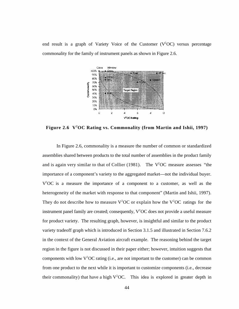
44
end result is a graph of Variety Voice of the Customer (V2OC) versus percentage
commonality for the family of instrument panels as shown in Figure 2.6.
Figure 2.6 V2OC Rating vs. Commonality (from Martin and Ishii, 1997)
In Figure 2.6, commonality is a measure the number of common or standardized
assemblies shared between products to the total number of assemblies in the product family
and is again very similar to that of Collier (1981). The V2OC measure assesses “the
importance of a component’s variety to the aggregated market—not the individual buyer.
V2OC is a measure the importance of a component to a customer, as well as the
heterogeneity of the market with response to that component” (Martin and Ishii, 1997).
They do not describe how to measure V2OC or explain how the V2OC ratings for the
instrument panel family are created; consequently, V2OC does not provide a useful measure
for product variety. The resulting graph, however, is insightful and similar to the product
variety tradeoff graph which is introduced in Section 3.1.5 and illustrated in Section 7.6.2
in the context of the General Aviation aircraft example. The reasoning behind the target
region in the figure is not discussed in their paper either; however, intuition suggests that
components with low V2OC rating (i.e., are not important to the customer) can be common
from one product to the next while it is important to customize components (i.e., decrease
their commonality) that have a high V2OC. This idea is explored in greater depth in

45
Sections 3.1.5 and 7.6.2 wherein a non-commonality index based on the dissimilarity of a
family of products defined by a parameter set is introduced for assessing and studying
product variety tradeoffs. In the meantime, methods for designing families of products are
reviewed in the next section.
2 .2 .3 Engineering Methods for Product Family Design
The majority of engineering design research has been directed at improving the
efficiency and effectiveness of designers in the product realization process, and until
recently, the focus has been on designing a single product. For instance, Suh (1990)
offers his two axioms for design: (1) maintain independence of functional requirements,
and (2) minimize the information content of a design. Pahl and Beitz (1988; 1996) offer
their four phase approach to product design which involves the following: clarification of
the task, conceptual design, embodiment design, and detail design. Similarly, Hubka and
Eder (1988; 1996) advocate an approach which involves the following: elaboration of the
assigned problem, conceptual design, laying out, and elaboration. Pugh (1991) introduces
the notion of total design which has at its core market/user needs and demands, the product
design specification, conceptual design, detail design, manufacturing, and selling. In the
well-known review of mechanical engineering design research conducted by Finger and
Dixon (1989a; 1989b), scant trace of product family and product platform design is found.
Perhaps the most developed method for product family design which currently
exists is the work by Erens (1997). Erens, in conjunction with several of his colleagues
(Erens and Breuls, 1995; Erens and Verhulst, 1997; Erens and Hegge, 1994; McKay, et
al., 1996), develops a product modeling language for product variety. The primary focus
is on the product modeling language as an efficient representation of product architecture
and modularity; it offers little aid for design synthesis and analysis, only representation.
The product modeling language allows product families to be represented in three domains:
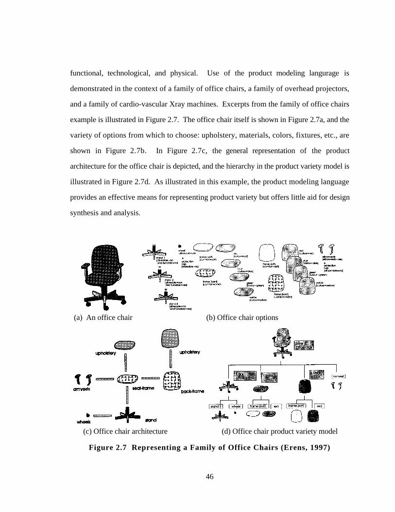
46
functional, technological, and physical. Use of the product modeling langurage is
demonstrated in the context of a family of office chairs, a family of overhead projectors,
and a family of cardio-vascular Xray machines. Excerpts from the family of office chairs
example is illustrated in Figure 2.7. The office chair itself is shown in Figure 2.7a, and the
variety of options from which to choose: upholstery, materials, colors, fixtures, etc., are
shown in Figure 2.7b. In Figure 2.7c, the general representation of the product
architecture for the office chair is depicted, and the hierarchy in the product variety model is
illustrated in Figure 2.7d. As illustrated in this example, the product modeling language
provides an effective means for representing product variety but offers little aid for design
synthesis and analysis.
(a) An office chair (b) Office chair options
(c) Office chair architecture (d) Office chair product variety model
Figure 2.7 Representing a Family of Office Chairs (Erens, 1997)
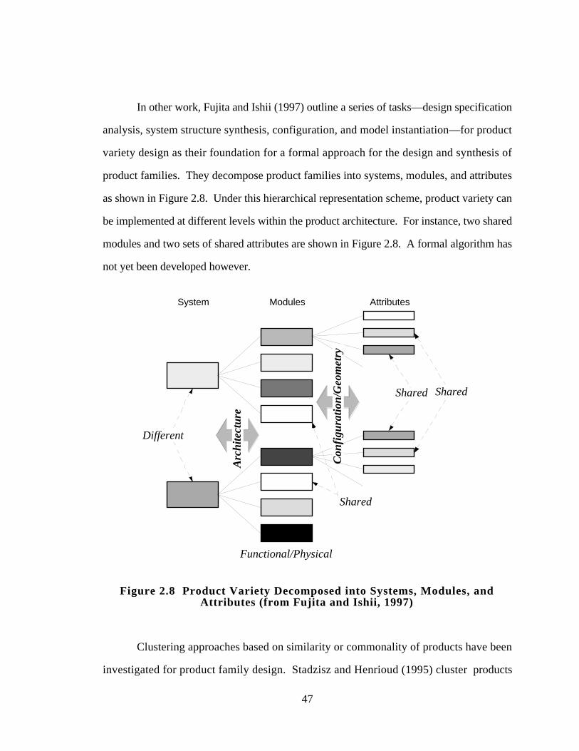
47
In other work, Fujita and Ishii (1997) outline a series of tasks—design specification
analysis, system structure synthesis, configuration, and model instantiation—for product
variety design as their foundation for a formal approach for the design and synthesis of
product families. They decompose product families into systems, modules, and attributes
as shown in Figure 2.8. Under this hierarchical representation scheme, product variety can
be implemented at different levels within the product architecture. For instance, two shared
modules and two sets of shared attributes are shown in Figure 2.8. A formal algorithm has
not yet been developed however.
System Modules Attributes
Shared
Con
figu
ratio
n/G
eom
etry
Arc
hite
ctur
e
Different
Shared Shared
Functional/Physical
Figure 2.8 Product Variety Decomposed into Systems, Modules, andAttributes (from Fujita and Ishii, 1997)
Clustering approaches based on similarity or commonality of products have been
investigated for product family design. Stadzisz and Henrioud (1995) cluster products
48
based on geometric similarities to obtain product families in order to decrease product
variability within a product family in order to minimize the required flexibility of the
associated assembly system. A similar Design for Mass Customization approach is
developed in (Tseng, et al., 1996) which groups similar products into families based on
product topology or manufacturing and assembly similarity and provides a series of steps
to formulate an optimal product family architecture based on grouping according to
fulfillment of functional requirements. Shirley (1990) describes a process for redesigning a
set of related products through similarity and clustering of common products around a
“core product concept,” i.e., a product platform. The resulting product family is composed
of a set of product variants which share characteristics in common with the core product;
the redesign of a family of hydraulic cylinders is used as an example.
Numerous researchers have focused on the implications of modularity on product
variety and in the context of a product platform and product family. Modularity greatly
facilitates the addition and removal of features to upgrade and derate a product platform
(cf., Ulrich, 1995). Ulrich and Tung (1991), Ulrich (1995), and Ulrich and Eppinger
(1995) investigate product architecture and modularity and its the impact on product
change, product variety, component standardization, product performance, and product
development management. Similarly, Uzumeri and Sanderson (1995) emphasize flexibility
and standardization as a means for enhancing product flexibility and offering a wide variety
of products. Meanwhile, Chen, et al. (1994) suggest designing flexible products which
can be adapted readily in response to large changes in customer requirements by changing a
small number of components or modules. Sanderson (1991) investigates how modular
designs reduce the cost of offering product variety. Rosen (1996) investigates the use of
discrete mathematics as a formal foundation for configuration design of modular product
architectures. He emphasizes, as do Ulrich and Eppinger (1995), that the design of
product architectures is “critical in being able to mass customize products to meet
49
differentiated market niches and satisfy requirements on local content, component carry-
over between generations, recyclability, and other strategic issues.” A Product Module
Reasoning System (Newcomb, et al., 1996) currently is being developed “to reason about
sets of product architectures, to translate design requirements into constraints on these sets,
to compare architecture modules from different viewpoints, and to directly enumerate all
feasible modules without generate-and-test or heuristic approaches” (Rosen, 1996).
Pahl and Beitz (1996) also discuss the advantages and limitations of modular
products to fulfill various overall functions through the combination of distinct modules.
Because such modules often come in various sizes, modular products often involve size
ranges where the initial size is the basic design and derivative sizes are sequential designs.
In the context of a scalable product platform, the initial size constitutes the product platform
and the derivative sizes are its product variants. Their approach for designing size ranges is
as follows (Pahl and Beitz, 1996):
• Prepare the basic design for the range either from a new or existing product;
• Use similarity laws to determine the physical relationships between geometrically
similar product ranges;
• Determine appropriate “theoretical” steps sizes within the desired size range;
• Adapt “theoretical” step sizes to overriding standards or technical requirements;
• Check the product size range against assembly layouts, checking any critical
dimensions; and
• Improve and document the design and prepare production drawings.
In the context of their approach, the method developed in this dissertation facilitates the
development of the basic design (i.e., the platform) and the sequential designs (i.e.,
derivative products) simultaneously.
The concept of sizing leads into an area of product platform design that has received
little attention—product platforms that can be “scaled” or “stretched” into derivative
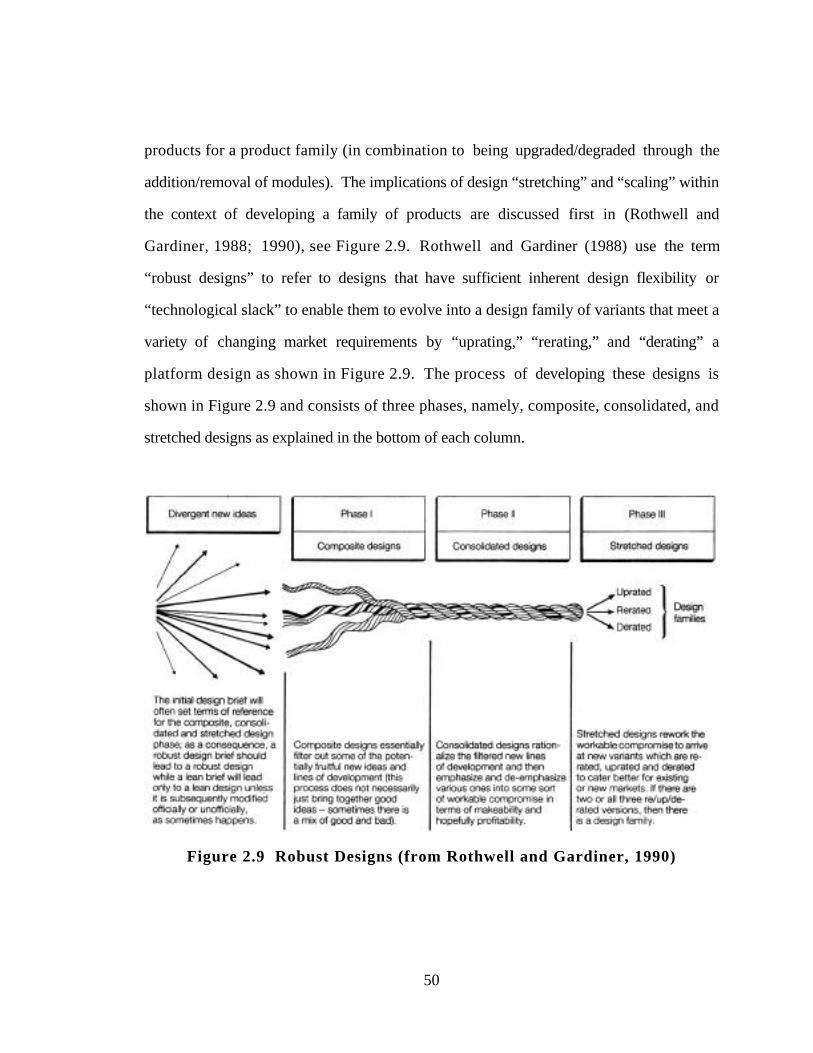
50
products for a product family (in combination to being upgraded/degraded through the
addition/removal of modules). The implications of design “stretching” and “scaling” within
the context of developing a family of products are discussed first in (Rothwell and
Gardiner, 1988; 1990), see Figure 2.9. Rothwell and Gardiner (1988) use the term
“robust designs” to refer to designs that have sufficient inherent design flexibility or
“technological slack” to enable them to evolve into a design family of variants that meet a
variety of changing market requirements by “uprating,” “rerating,” and “derating” a
platform design as shown in Figure 2.9. The process of developing these designs is
shown in Figure 2.9 and consists of three phases, namely, composite, consolidated, and
stretched designs as explained in the bottom of each column.
Figure 2.9 Robust Designs (from Rothwell and Gardiner, 1990)
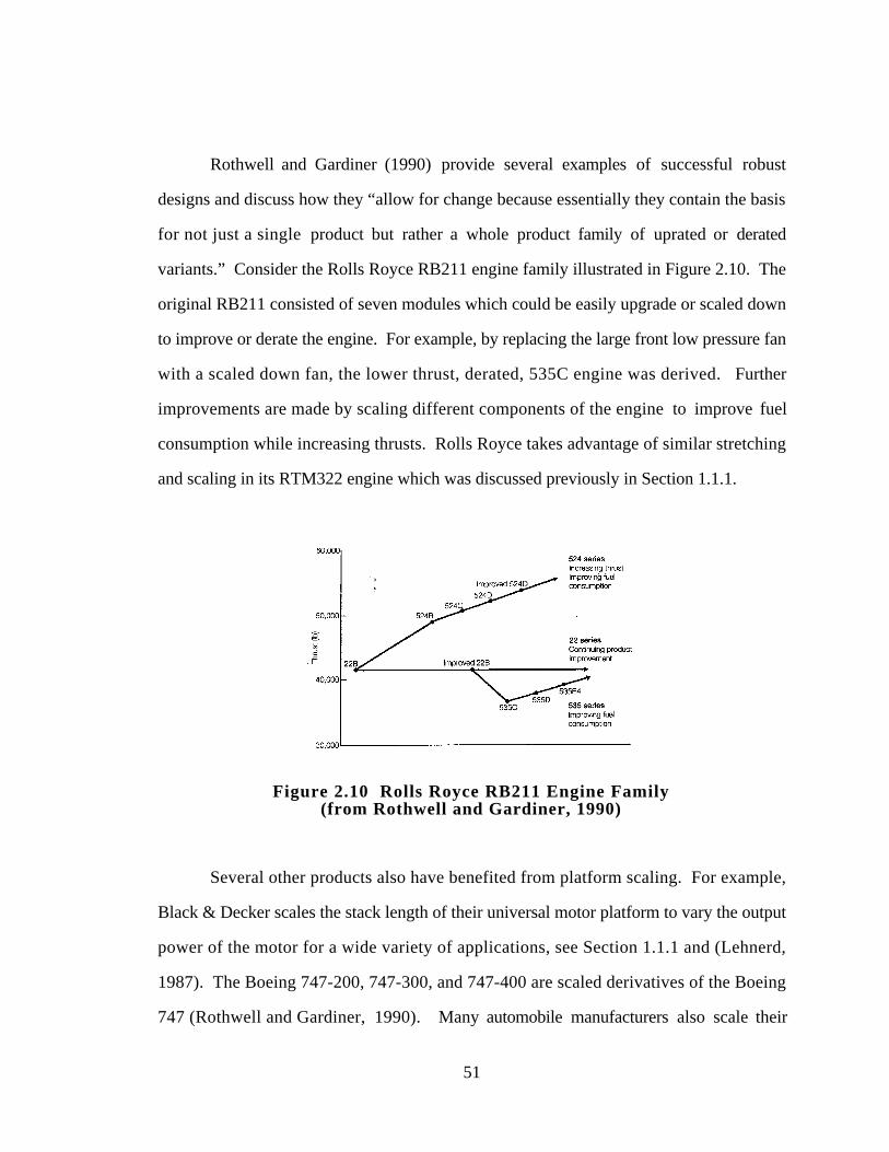
51
Rothwell and Gardiner (1990) provide several examples of successful robust
designs and discuss how they “allow for change because essentially they contain the basis
for not just a single product but rather a whole product family of uprated or derated
variants.” Consider the Rolls Royce RB211 engine family illustrated in Figure 2.10. The
original RB211 consisted of seven modules which could be easily upgrade or scaled down
to improve or derate the engine. For example, by replacing the large front low pressure fan
with a scaled down fan, the lower thrust, derated, 535C engine was derived. Further
improvements are made by scaling different components of the engine to improve fuel
consumption while increasing thrusts. Rolls Royce takes advantage of similar stretching
and scaling in its RTM322 engine which was discussed previously in Section 1.1.1.
Figure 2.10 Rolls Royce RB211 Engine Family(from Rothwell and Gardiner, 1990)
Several other products also have benefited from platform scaling. For example,
Black & Decker scales the stack length of their universal motor platform to vary the output
power of the motor for a wide variety of applications, see Section 1.1.1 and (Lehnerd,
1987). The Boeing 747-200, 747-300, and 747-400 are scaled derivatives of the Boeing
747 (Rothwell and Gardiner, 1990). Many automobile manufacturers also scale their
52
passenger car platforms to offer, for example, two-door coupes, two- and four-door
sedans, three- and five-door hatchbacks, and maybe a wagon which are all derived from
the same platform (Rothwell and Gardiner, 1990). Honda, for instance, is taking full
advantage of platform scaling to compete in today’s global market by developing two
scaled versions of their Accord for the U.S. and Japanese markets from one platform
(Naughton, et al., 1997). Siddique, et al. (1998) document efforts at Ford to improve the
commonality of their product platforms to capitalize on commonality and stretching within
their automotive product families.
Despite the apparent advantages of scalable product platforms, a formal approach
for the design and synthesis of stretchable and scalable platforms does not exist. Rothwell
and Gardiner state that it has “become increasingly possible to develop a robust design
which has the deliberate designed-in capability of being stretched;” however, they only
offer the process shown in Figure 2.9 as a guide to designers. Consequently, developing a
method to model and design scalable product platforms around which a family of products
can be developed through scaled derivatives of the product platform is the principal
objective in this dissertation. In an effort to realize such a method, an extension of robust
design principles is offered in the next section, providing a means to turn Rothwell and
Gardiner’s idea of “robust design” for scalable product platforms into a reality.
2.3 ROBUST DESIGN
Generally speaking, the fundamental motive underlying robust design, as originally
proposed by Taguchi, is to improve the quality of a product or process by not only striving
to achieve performance targets but also by minimizing performance variation. Taguchi’s
methods have been widely used in industry (see, e.g., Byrne and Taguchi, 1987; Phadke,
1989) for parameter and tolerance design. Reviews of such applications can be found in,
e.g., (Nair, 1992).
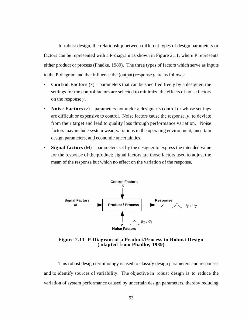
53
In robust design, the relationship between different types of design parameters or
factors can be represented with a P-diagram as shown in Figure 2.11, where P represents
either product or process (Phadke, 1989). The three types of factors which serve as inputs
to the P-diagram and that influence the (output) response y are as follows:
• Control Factors (x) – parameters that can be specified freely by a designer; the
settings for the control factors are selected to minimize the effects of noise factors
on the response y.
• Noise Factors (z) – parameters not under a designer’s control or whose settings
are difficult or expensive to control. Noise factors cause the response, y, to deviate
from their target and lead to quality loss through performance variation. Noise
factors may include system wear, variations in the operating environment, uncertain
design parameters, and economic uncertainties.
• Signal factors (M) – parameters set by the designer to express the intended value
for the response of the product; signal factors are those factors used to adjust the
mean of the response but which no effect on the variation of the response.
Product / Process
Noise Factors
ResponseSignal Factors
Control Factorsx
z
M y
µz , σz
µy , σy
Figure 2.11 P-Diagram of a Product/Process in Robust Design(adapted from Phadke, 1989)
This robust design terminology is used to classify design parameters and responses
and to identify sources of variability. The objective in robust design is to reduce the
variation of system performance caused by uncertain design parameters, thereby reducing

54
system sensitivity. Variations in noise factors, shown in Figure 2.11 as normally
distributed with mean µz and standard deviation σz, lead to variation in performance
responses, which are represented in Figure 2.11 as normally distributed with mean µy and
standard deviation σy.
In an effort to generalize robust design for product design, Chen, et al. (1996a)
develop a general robust design procedure based on two sources of variation:
Type I - Robust design associated with the minimization of the deviation of
performance caused by the deviation of noise factors (uncontrollable parameters).
Type II - Robust design associated with the minimization of the deviation of
performance caused by the deviation of control factors (design variables).
The idea behind the two major types of robust design applications are illustrated in Figure
2.12. As indicated by the P-diagrams for Type I and Type II applications, the deviation of
the response is caused by variations in the noise factor, z, the uncontrollable parameter in
Type I applications. Type II is different from Type I in that its input does not include a
noise factor. The variation in performance is caused solely by variations in control factors
or design variables in the region ±∆x.
The traditional Taguchi robust design method is of Type I as shown in the top half
of Figure 2.12. A designer adjusts control factors, x , to dampen the variations caused by
the noise factor, z . The two curves represent the performance variation as a function of
noise factor when x is at two different levels, x = a and x = b. If the design objective is to
achieve a performance as closely as possible to the target, M, the designs at both levels are
acceptable because their means are the target M. However, introducing robustness, when
x = a, the performance varies significantly with the deviation of noise factor, z ; however,
when x = b, the performance deviates much less. Therefore, x = b is more robust than x
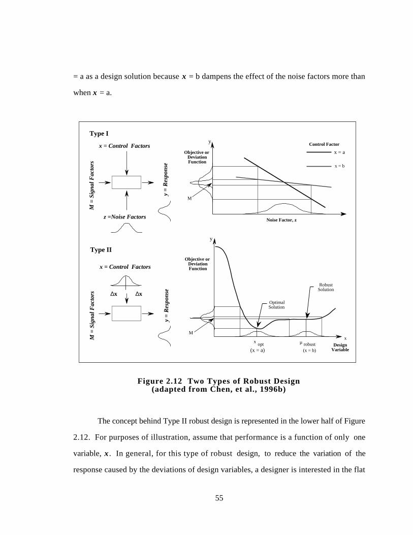
55
= a as a design solution because x = b dampens the effect of the noise factors more than
when x = a.
y =
Res
pons
e
M =
Sig
nal F
acto
rs
x = Control Factors
z =Noise Factors
Type I
x = Control Factors
M =
Sig
nal F
acto
rs
Type II
y =
Res
pons
e
∆x∆x
y
xrobustµ
M
OptimalSolution
RobustSolution
DesignVariable
Objective orDeviationFunction
optx
Noise Factor, z
x = a
x = b
M
Control Factor
Objective orDeviationFunction
y
(x = b)(x = a)
Figure 2.12 Two Types of Robust Design(adapted from Chen, et al., 1996b)
The concept behind Type II robust design is represented in the lower half of Figure
2.12. For purposes of illustration, assume that performance is a function of only one
variable, x . In general, for this type of robust design, to reduce the variation of the
response caused by the deviations of design variables, a designer is interested in the flat
56
part of a curve near the performance target instead of seeking the peak or optimum value.
If the objective is to move the performance function towards target M and if a robust design
is not sought, then the point x = a is chosen. However, for a robust design, x = b is a
better choice. This is because if the design variable varies within ±∆x of its mean, the
resulting variation of response of the design at x = b is much smaller than that at x = a,
while the means of the two responses are essentially equal. Implementation of these two
types of robust design are discussed in the next section.
2 .3 .1 Implementation of Robust Design: Taguchi’s Method, in the RobustConcept Exploration Method, and with Design Capability Indices
Design of experiments, specifically orthogonal arrays (OA), are typically employed in
Taguchi’s robust design method to systematically vary and test the different levels of each
of the control factors. Taguchi advocates the use of an inner-array and outer-array
approach to implement robust design (cf., e.g., Byrne and Taguchi, 1987). The inner-
array consists of an OA which contains the control factor settings; the outer-array consists
of the OA which contains the noise factors and their settings which are under investigation.
The combination of the inner-array and outer-array constitutes the product array. The
product array is used to test various combinations of the control factor settings
systematically over all combinations of noise factors after which the mean response and
standard deviation may be approximated for each run using the equations:
• Response mean: y =1
nyi
i =1
n
∑ [2.3]
• Standard deviation: S =(y i − y )2
n −1i=1
n
∑ [2.4]
57
Preferred parameter values then can be determined through analysis of the signal-to-noise
(SN) ratio; factor levels that maximize the appropriate SN ratio are optimal. There are three
“standard” types of SN ratios (see, e.g., Phadke, 1989):
• Nominal the best (for reducing variability around a target):
SNT = 10logy 2
S2
[2.5]
• Smaller the better (for making the system response as small as possible):
SNL = −10log1
n
1
yi2
i =1
n
∑
[2.6]
• Larger the better (for making the system response as large as possible):
SNS =− 10log1
ny i
2
i =1
n
∑
[2.7]
Once all of the SN ratios have been computed for each run of an experiment, there
are two common options for analysis: Analysis of Variance (ANOVA) and a graphical
approach. ANOVA can be used to determine the statistically significant factors and the
appropriate setting for each. In the graphical approach, the SN ratios and average
responses are plotted for each factor against its levels. The graphs then are examined to
“pick the winner,” i.e., pick the factor levels which (1) best maximize SN and (2) bring the
mean on target (or maximize or minimize the mean, as the case may be).
There are many criticisms of Taguchi’s implementation of robust design through the
inner and outer array approach: it requires too many experiments, the analysis is statistically
questionable because of the use of orthogonal arrays, it does not accommodate constraints,
and the responses should be modeled directly instead of the SN ratios (see, e.g.,
58
Montgomery, 1991; Nair, 1992; Otto and Antonsson, 1993; Shoemaker, et al., 1991;
Tribus and Szonyi, 1989; Tsui, 1992). Consequently many variations of the Taguchi
method have been proposed and developed; a review of numerous robust design
optimization methods can be found in (Otto and Antonsson, 1993; Simpson, et al., 1997a;
Simpson, et al., 1997b; Su and Renaud, 1996; Tsui, 1992; Yu and Ishii, 1998).
To facilitate the implementation of robust design within the RCEM, second-order
response surface models are created and used to approximate the design space, replacing
the computer analysis code or simulation routine used to model the system. The major
elements of the response surface model approach for robust design applications are as
follows (see, e.g., Myers and Montgomery, 1995; Shoemaker, et al., 1991):
• combining control and noise factors in a single array instead of using Taguchi's
inner- and outer-array approach,
• modeling the response itself rather than expected loss, and
• approximating a prediction model for loss based on the fitted-response model.
Instead of using Taguchi’s orthogonal array as the combined array for experiments, central
composite designs are employed in the RCEM to fit second-order response surface models
for integration with Taguchi's robust design. The response surface model postulates a
single, formal model of the type:
ˆ y = f(x ,z) [2.8]
where ˆ y is the estimated response and x and z represent the settings of the control and
noise variables, respectively. In Equation 2.8, it is assumed that the noise variables are
independent. From the response surface model, it is possible to estimate the mean and
variance of the response. For Type I applications in which the deviations of noise factors
are the source of variation:
59
• Mean of response: µ ˆ y = f(x ,µz) [2.9]
• Variance of response: σ ˆ y 2 =
∂f
∂z i
2
i =1
m
∑ σ z i
2 [2.10]
where µ represents the mean values, m is the number of noise factors in the response
model, and σ z i is the standard deviation associated with each noise factor. In Type II
robust design, i.e., when the deviations of control factors are the source of variation, µz
and σ z i in Equations 2.9-2.10 are replaced by the mean and deviation of the variable
control factors. Using this approach, robust design can be achieved by having separate
goals for “bringing the mean on target” and “minimizing the deviation” within a
compromise DSP (cf., Chen, et al., 1996b).
When satisfying the design requirements and reducing the variation of system
performance are equally important, it is effective to model the two aspects of robust design
as separate goals in the compromise DSP. For instance, when designing a power plant, it
may be required to bring the power output as close as possible to its target value while at
the same time, reduce the variation of the system performance so that the power output
remains constant during operation. Moreover, setting an overall design requirement at a
specific value during the early stages of design may sometimes be crucial because a small
variation may require significant changes in other design requirements or incur substantial
costs in order to compensate for it. However, modeling the two aspects of robust design
as two separate goals may not be an effective approach when satisfying a range of design
requirements is the major concern, see Figure 2.13.
In Figure 2.13, the quality distributions of two different designs (I and II) are
illustrated. Both designs have the same mean value but different deviations. If the two
aspects of robust design are modeled as separate goals, obviously the design with the least
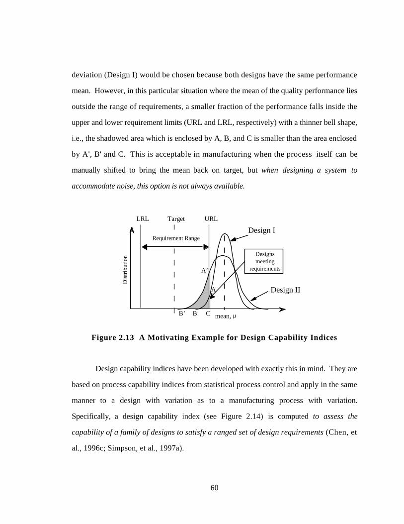
60
deviation (Design I) would be chosen because both designs have the same performance
mean. However, in this particular situation where the mean of the quality performance lies
outside the range of requirements, a smaller fraction of the performance falls inside the
upper and lower requirement limits (URL and LRL, respectively) with a thinner bell shape,
i.e., the shadowed area which is enclosed by A, B, and C is smaller than the area enclosed
by A', B' and C. This is acceptable in manufacturing when the process itself can be
manually shifted to bring the mean back on target, but when designing a system to
accommodate noise, this option is not always available.
URLLRL Target
mean, µ
Requirement Range
Dis
trib
utio
n
A
A’
BB’ C
Design II
Design I
Designs meeting
requirements
Figure 2.13 A Motivating Example for Design Capability Indices
Design capability indices have been developed with exactly this in mind. They are
based on process capability indices from statistical process control and apply in the same
manner to a design with variation as to a manufacturing process with variation.
Specifically, a design capability index (see Figure 2.14) is computed to assess the
capability of a family of designs to satisfy a ranged set of design requirements (Chen, et
al., 1996c; Simpson, et al., 1997a).
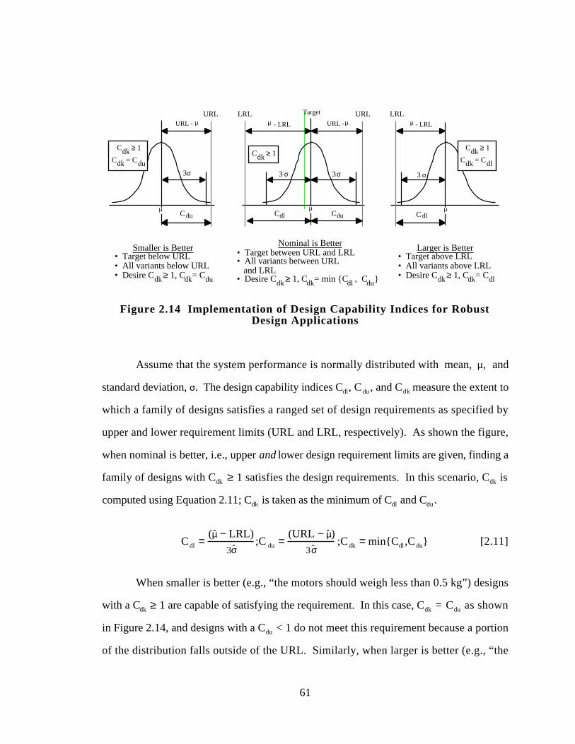
61
3 σ
LRL
C dlµ
- LRLµURL
C du
URL - µ
µ
3σ
LRL URLTarget
Cdl Cdu
- LRLµ URL - µ
3σ3 σ
C ≥ 1dk
µ
Larger is Better• Target above LRL• All variants above LRL• Desire C ≥ 1, C = C
Smaller is Better• Target below URL• All variants below URL• Desire C ≥ 1, C = Cdk
Nominal is Better• Target between URL and LRL• All variants between URL and LRL• Desire C ≥ 1, C = min {C , C }dk
C ≥ 1dkC = Cdudk
C ≥ 1dkC = Cdldk
dk du dk dk dldudldk
Figure 2.14 Implementation of Design Capability Indices for RobustDesign Applications
Assume that the system performance is normally distributed with mean, µ, and
standard deviation, σ. The design capability indices Cdl, Cdu , and Cdk measure the extent to
which a family of designs satisfies a ranged set of design requirements as specified by
upper and lower requirement limits (URL and LRL, respectively). As shown the figure,
when nominal is better, i.e., upper and lower design requirement limits are given, finding a
family of designs with Cdk ≥ 1 satisfies the design requirements. In this scenario, Cdk is
computed using Equation 2.11; Cdk is taken as the minimum of Cdl and Cdu .
Cdl =(ˆ µ − LRL)
3ˆ σ ;C du =
(URL − ˆ µ )
3ˆ σ ;Cdk = min{Cdl ,Cdu} [2.11]
When smaller is better (e.g., “the motors should weigh less than 0.5 kg”) designs
with a Cdk ≥ 1 are capable of satisfying the requirement. In this case, Cdk = Cdu as shown
in Figure 2.14, and designs with a Cdu < 1 do not meet this requirement because a portion
of the distribution falls outside of the URL. Similarly, when larger is better (e.g., “the
62
efficiency of these motors should be 30% or better”), designs with a Cdk ≥ 1 are capable of
meeting this requirement; Cdk = Cdl.
There are some assumptions associated with the use of Cdk . For example, Cdk = 1
implies only 99.73% of the designs conform to requirements assuming that the system
performance parameters—which are based on the range of designs—are normally
distributed. However, the type of distribution of system performance depends on the
actual system response and the statistical distribution of each design variable or uncertainty
parameter. When the system function is complex, it may be difficult to perform a judicious
evaluation to determine performance distribution. As an approximation, if it is assumed
that the uncertain parameters deviate by ±3σz (as is typical in a six sigma approach to
quality) around their nominal value µz, and that each system response varies by ±3σy
around its mean value, µy, which can be calculated by:
µy = y (µx) [2.12]
The standard deviation, σy, is approximated using a first order Taylor series expansion
(assuming σx is small):
ˆ σ y2 =
∂y
∂z i
2
i =1
m
∑ σ z2 [2.13]
Modifications to the process capability indices for different variances have been
proposed (see, e.g., Johnson, et al., 1992; Ng and Tsui, 1992; Rodriguez, 1992), and
design capability indices could be modified similarly. For example, if a uniform
distribution is used for each response instead of a normal distribution, then Cdk , Cdu , and
Cdl become as follows:
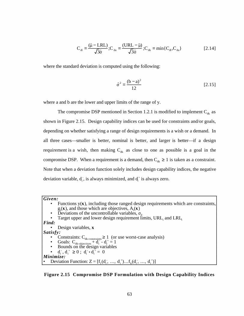
63
Cdl =(ˆ µ − LRL)
3ˆ σ ;C du =
(URL − ˆ µ )
3 ˆ σ ;Cdk = min{Cdl ,Cdu} [2.14]
where the standard deviation is computed using the following:
ˆ σ 2 =(b − a)2
12[2.15]
where a and b are the lower and upper limits of the range of y.
The compromise DSP mentioned in Section 1.2.1 is modified to implement Cdk as
shown in Figure 2.15. Design capability indices can be used for constraints and/or goals,
depending on whether satisfying a range of design requirements is a wish or a demand. In
all three cases—smaller is better, nominal is better, and larger is better—if a design
requirement is a wish, then making Cdk as close to one as possible is a goal in the
compromise DSP. When a requirement is a demand, then Cdk ≥ 1 is taken as a constraint.
Note that when a deviation function solely includes design capability indices, the negative
deviation variable, di-, is always minimized, and di
+ is always zero.
Given:• Functions y(x), including those ranged design requirements which are constraints,
gi(x), and those which are objectives, Ai(x)• Deviations of the uncontrollable variables, σZ • Target upper and lower design requirement limits, URLi and LRLi
Find:• Design variables, x
Satisfy:• Constraints: Cdk-constraints ≥ 1 (or use worst-case analysis)• Goals: Cdk-objectives + di
- - di+ = 1
• Bounds on the design variables• di
- , d i+ ≥ 0 ; di
- • di+ = 0
Minimize:• Deviation Function: Z = [f1(di
-, ..., d i+)...fk(di
-, ..., d i+)]
Figure 2.15 Compromise DSP Formulation with Design Capability Indices
64
Working with these two types of robust design implementations, it is possible to
develop an extension for product family design, specifically for scalable product platforms,
which addresses the question:
Q1.2. How can robust design principles be used to facilitate the design a common
scalable product platform?
Extensions of robust design for product family design are discussed in the next section.
2 .3 .2 Robust Design for Product Family Design: Scale Factors
There have been two known allusions to using robust design in product family
design. First, Lucas (1994) describes a way that the results of a robust design experiment
can be used to identify the need for product differentiation. When large effects are present
in the system, different product types can be sent to customers having different features as
opposed to designing one product which is robust over the entire range of effects. He
states that this is common practice in the chemical industry where, for example, different
polymer viscosities are desired by different customers and better results often are obtained
by customizing the product for its specific environment rather than delivering a single
robust product.
Second, Chang, et al. (1994) and Chang and Ward (1995) introduce the notion of
“conceptual robustness” which is pertinent to this research. The term “conceptual
robustness” is developed by Chang and his colleagues for mathematically modeling and
computationally supporting simultaneous (or concurrent) engineering in a distributed
design environment. By treating variations in the design proposed by other members of the
development team as “conceptual noise,” robust design principles can be used to make
“conceptually robust” decisions which are robust against these variations (Chang, et al.,
65
1994). The “conceptually robust” design of a two-axis CNC milling machine is used as an
illustrative example. In (Chang and Ward, 1995), this idea is applied to modular design
which is a “function-oriented design that can be integrated into different systems for the
same functional purpose without (or with minor) modifications.” The design of an air
conditioning system for ten different automobiles is used to demonstrate their approach.
It is this idea of a “conceptual noise factor” that enables the utilization of robust
design in the context of product family design, particularly in the design of a scalable
product platform. By identifying an appropriate “scale factor” for a scalable product
platform, robust design principles can be used to minimize the sensitivity of the product
platform to variations in a scale factor. In this regard, a “conceptually robust” product
platform can be realized which has minimum sensitivity to variations in the scale factor,
realizing a robust product family. For the work in this dissertation, then, a scale factor is
defined as follows:
• Scale factor - factor around which a product platform can be “scaled” or
“stretched” to realize derivative products within a product family.
In essence, a scale factor is a noise factor within a scalable product family or, to
borrow terminology from Chang, et al. (1994)), a “conceptual noise factor” around which
a “conceptually robust” product platform can be developed for a product family. Examples
of scale factors include the stack length in a motor, as in the Black & Decker universal
motor example (Lehnerd, 1987), the number of passengers on an aircraft ,as in the Boeing
747 family (Rothwell and Gardiner, 1990), or the number of compressor stages in an
aircraft engine, as in the Rolls Royce RTM322 example (Rothwell and Gardiner, 1990).
Scale factors may be either discrete or continuous; however, continuous scale factors are
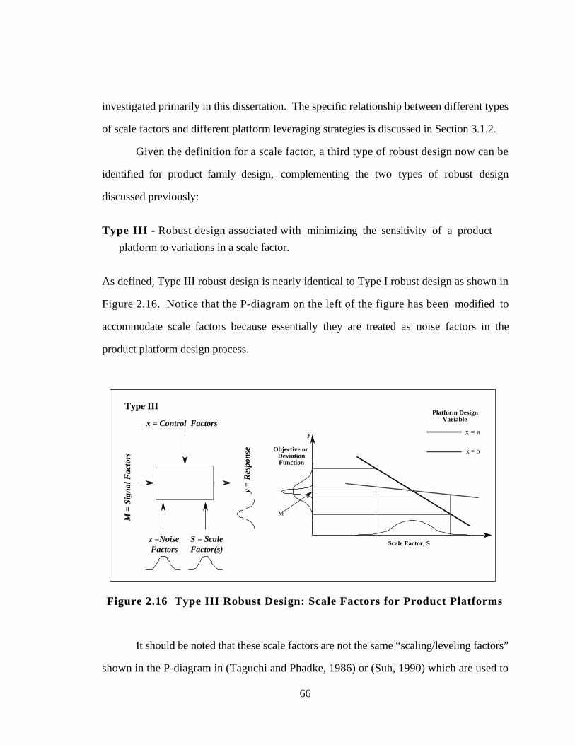
66
investigated primarily in this dissertation. The specific relationship between different types
of scale factors and different platform leveraging strategies is discussed in Section 3.1.2.
Given the definition for a scale factor, a third type of robust design now can be
identified for product family design, complementing the two types of robust design
discussed previously:
Type III - Robust design associated with minimizing the sensitivity of a product
platform to variations in a scale factor.
As defined, Type III robust design is nearly identical to Type I robust design as shown in
Figure 2.16. Notice that the P-diagram on the left of the figure has been modified to
accommodate scale factors because essentially they are treated as noise factors in the
product platform design process.
y =
Res
pons
e
M =
Sig
nal F
acto
rs
x = Control Factors
S = ScaleFactor(s)
Type III
Scale Factor, S
x = a
x = b
M
Platform DesignVariable
Objective orDeviationFunction
y
z =NoiseFactors
Figure 2.16 Type III Robust Design: Scale Factors for Product Platforms
It should be noted that these scale factors are not the same “scaling/leveling factors”
shown in the P-diagram in (Taguchi and Phadke, 1986) or (Suh, 1990) which are used to
67
scale a response to achieve a desired value. Using the same diagram shown in Figure 2.12
for the Type I robust design, the idea behind Type III robust design is illustrated in the
right hand side of Figure 2.16. Given two possible settings (x = a and x = b) for one of
the design variables, x, which defines the platform, the setting x = b should be selected
because it minimizes the sensitivity of the product platform to variations in the scale factor.
Consequently, if a family of products can be leveraged or scaled around an
identifiable scale factor, then robust design can be used to minimize the sensitivity of the
product platform to changes in these scaling factors. In this manner, a scalable product
platform can be developed and instantiated to realize a family of products. This raises the
following question then.
Q1.3. How can individual targets for product variants be aggregated and modeled
for product platform design?
Using the concept of a scale factor for a product platform, it is now possible to
aggregate the individual targets for product variants within a product family around an
appropriate mean and a standard deviation. Robust design principles then can be used to
“match” the mean and standard deviation of the product family with the desired mean and
standard deviation of the performance requirements by either of the following as discussed
in Section 2.3.1:
• creating separate goals for “bringing the mean on target” and “minimizing the
deviation” of the product platform for variations in the scale factor within a
compromise DSP, or
• using design capability indices to assess the capability of a family of designs to
satisfy a ranged set of design requirements.
To demonstrate these implementations, the former approach is utilized in the universal
electric motor problem in Chapter 6; the latter is employed in the General Aviation aircraft
68
example in Chapter 7. The General Aviation aircraft example also makes use of
metamodels to facilitate the implementation of robust design and design capability indices
and expedite the concept exploration process as mentioned earlier. Metamodeling
techniques are discussed next.
2.4 METAMODELING TECHNIQUES
To facilitate the implementation of robust design, metamodeling techniques often
are employed to create approximations of the mean and variation of a response in the
presence of noise. A metamodel is a “model of a model” (Kleijnen, 1987) which is used as
a surrogate approximation for the actual analysis (i.e., computer code) during the design
process. The general approach to response surface modeling is shown in Figure 2.17. In
statistical terms, design variables are factors, and design objectives are responses; the
factors and responses to be investigated for a particular design problem provide the input
for the approach of Figure 2.17, and the solutions (improved or robust) are the output. To
identify these solutions, this approach includes three sequential stages: screening, modeling
building, and model exercising.
The first step (screening) is employed only if the problem includes a large number
of factors (usually greater than 10); screening experiments are used to reduce the set of
factors to those that are most important to the response(s) being investigated. Statistical
experimentation is used to define the appropriate design analyses which must be run to
evaluate the desired effects of the factors. Often two level fractional factorial designs or
Plackett-Burman designs are used for screening (cf., Myers and Montgomery, 1995), and
only main (linear) effects of each factor are investigated.
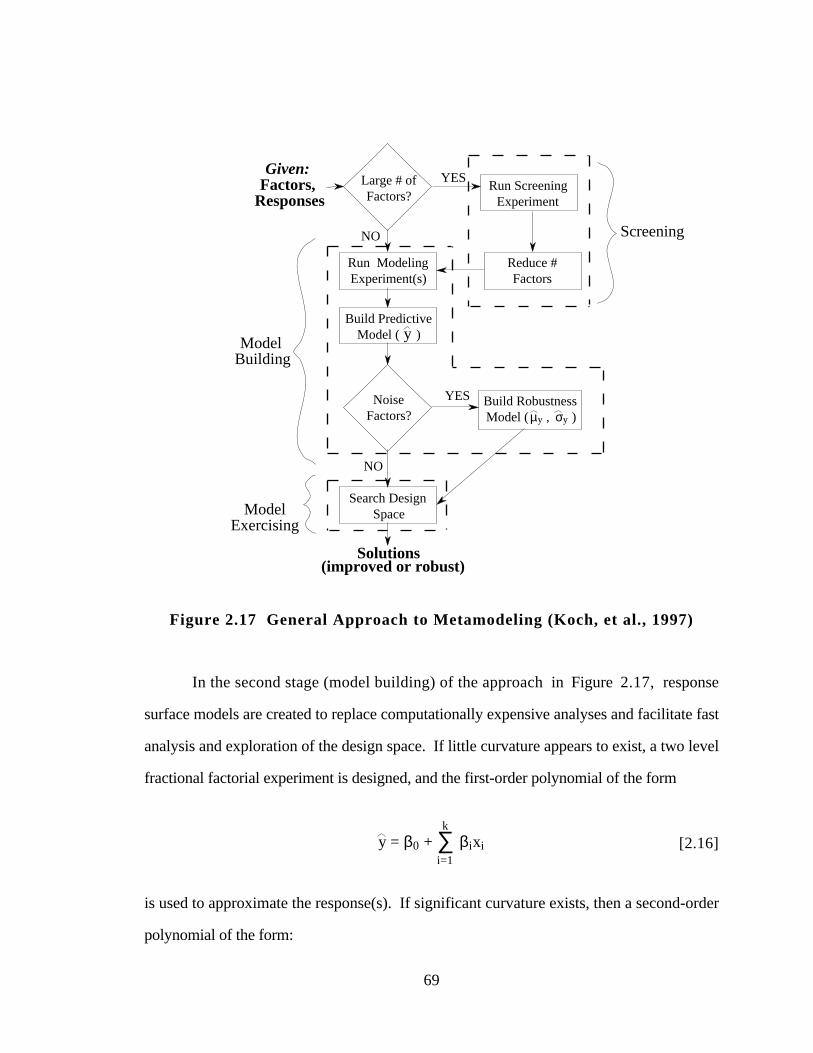
69
YESLarge # of Factors?
Run Screening Experiment
Reduce #Factors
Run Modeling Experiment(s)
Build Predictive Model ( )
Solutions
Search Design Space
NO
Given: Factors,
Responses
y
YES
NO
NoiseFactors?
Build Robustness Model ( )
Screening
Model Building
ModelExercising
(improved or robust)
µy , σy
Figure 2.17 General Approach to Metamodeling (Koch, et al., 1997)
In the second stage (model building) of the approach in Figure 2.17, response
surface models are created to replace computationally expensive analyses and facilitate fast
analysis and exploration of the design space. If little curvature appears to exist, a two level
fractional factorial experiment is designed, and the first-order polynomial of the form
y = β0 + βixi∑i=1
k
[2.16]
is used to approximate the response(s). If significant curvature exists, then a second-order
polynomial of the form:
70
y = β0 + βixi∑i=1
k
+ βiixi 2∑
i=1
k
+ βijxixj∑j
∑i
[2.17]
i<j
is commonly used. Among the various types of experimental design for fitting a second-
order response surface model, the central composite design (CCD) is probably the most
widely used experimental design for regularly shaped (spherical or cuboidal) design spaces
(cf., Myers and Montgomery, 1995). In the case of irregularly shaped design spaces, D-
optimal designs have been successfully employed to build second order response surface
models (see, e.g., Giunta, et al., 1994).
If noise factors are included for robust design, the mean and variance of each
response must be estimated, and predictive metamodels for both are constructed. As
discussed in (Koch, et al., 1998), there are essentially three approaches which can be
employed to construct metamodels for robust design applications:
1. Statistical expected value and Taylor series expansion approximations: A single
experimental design is created which contains both control and noise factors from
which a response surface model is built (see, e.g., Chen, et al., 1996b; Shoemaker,
et al., 1991). The mean value of a response is estimated by evaluating the response
surface at the mean of the noise factor, and the variance is estimated using a Taylor
series approximation. This is the approach currently employed in the RCEM as
described previously in Section 2.3.1.
2. DOE-based Monte Carlo simulation approach: A combined response surface and
Monte Carlo simulation approach is used to create mean and variance metamodels
(see, e.g., Mavris, et al., 1996; Mavris, et al., 1995). An initial experiment is
constructed to vary both control and noise factors and build response surface
models of each response similar to the first approach. A second experiment is
created to vary only the control factors, running a Monte Carlo simulation for each
experiment to vary the noise factors. Approximations for mean and variance are
constructed based on this second set of experiments.
71
3. Product array approach: Uses the inner- and outer-array approach advocated by
Taguchi (see, e.g., Montgomery, 1991; Phadke, 1989) to develop separate
approximations for the mean and variance of each response. The inner-array
prescribes settings for the control factors, and the outer-array prescribes settings for
the noise factors. This experimentation strategy leads to multiple response values
for each set of control factor settings from which a response mean and variance can
be computed from which metamodels can be constructed.
Of the three approaches, the product array approach typically yields the most accurate
approximations because the metamodels are built directly from the original analysis code
rather than from an estimate based on an approximation (cf., Koch, et al., 1998).
As shown in Figure 2.17 and as evidenced by the preceding discussion, building
approximations of computer analysis and simulation codes involves the following: (a)
choosing an experimental design to sample the computer code, (b) choosing a model to
represent the data, and (c) fitting the model to the observed data. There are a variety of
options for each of these steps as shown in Figure 2.18, and some of the more prevalent
approximation techniques have been identified. For example, response surface
methodology usually employs central composite designs, second-order polynomials, and
least squares regression analysis. The reader is referred to (Simpson, et al., 1997b) for a
recent review of numerous mechanical and aerospace engineering applications of many of
the metamodeling techniques shown in Figure 2.18 with particular emphasis on response
surface methodology, neural networks, inductive learning, and kriging.
By far the most popular technique for building metamodels these days is the
response surface approach which typically employs second-order polynomial models fit
using least squares regression techniques (Myers and Montgomery, 1995). These
response surface models replace the existing analysis code while providing the following:
• an understanding of the relationship between (input) design variables x and (output)
responses y ,
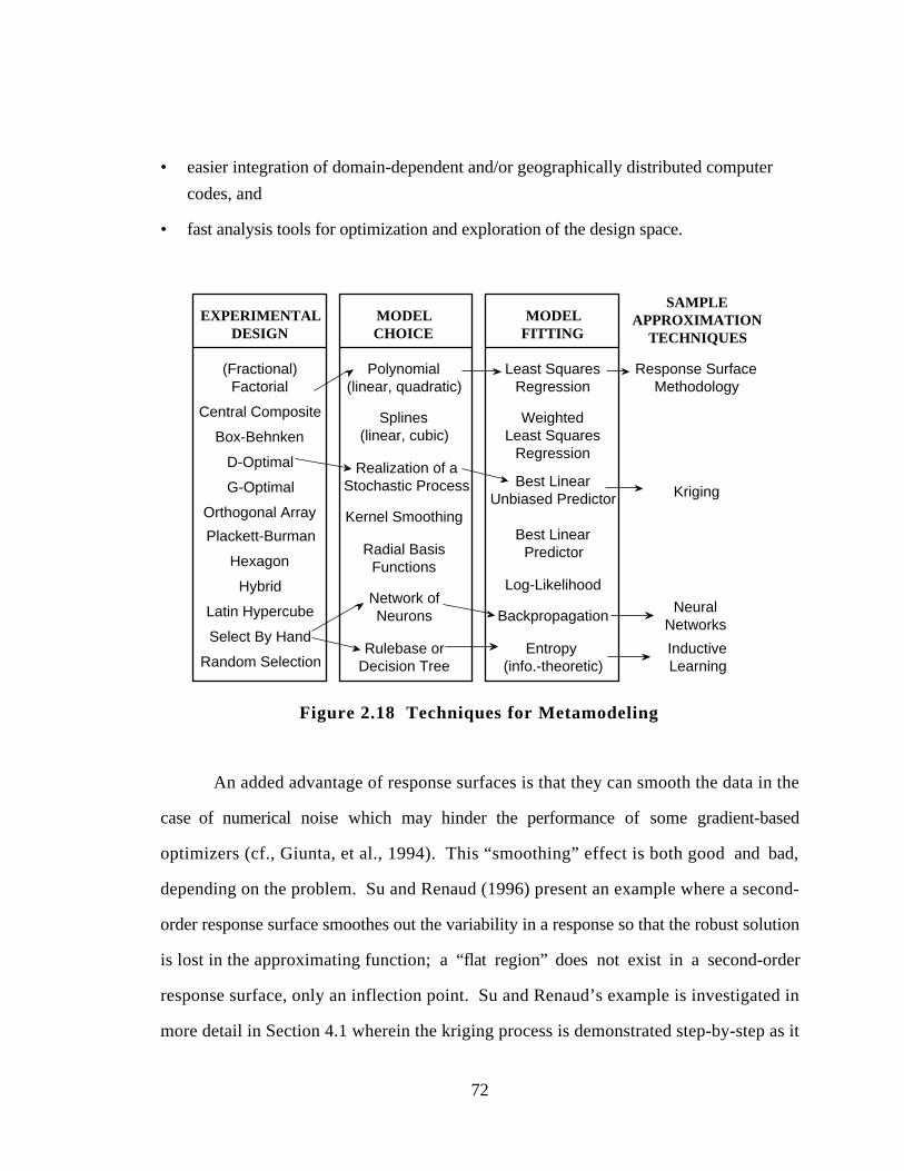
72
• easier integration of domain-dependent and/or geographically distributed computer
codes, and
• fast analysis tools for optimization and exploration of the design space.
Best LinearUnbiased Predictor
Realization of aStochastic Process
SAMPLE APPROXIMATION
TECHNIQUES
MODELFITTING
EXPERIMENTALDESIGN
MODELCHOICE
Kriging
NeuralNetworks
InductiveLearning
(Fractional) Factorial
Central Composite
Box-Behnken
Latin Hypercube
D-Optimal
Plackett-Burman
Hexagon
Hybrid
Polynomial(linear, quadratic)
Splines(linear, cubic)
Network ofNeurons
Rulebase orDecision Tree
Radial BasisFunctions
Kernel Smoothing
Least SquaresRegression
WeightedLeast Squares
Regression
Backpropagation
Entropy (info.-theoretic) Random Selection
Select By Hand
Log-Likelihood
G-Optimal
Orthogonal Array
Best LinearPredictor
Response Surface Methodology
Figure 2.18 Techniques for Metamodeling
An added advantage of response surfaces is that they can smooth the data in the
case of numerical noise which may hinder the performance of some gradient-based
optimizers (cf., Giunta, et al., 1994). This “smoothing” effect is both good and bad,
depending on the problem. Su and Renaud (1996) present an example where a second-
order response surface smoothes out the variability in a response so that the robust solution
is lost in the approximating function; a “flat region” does not exist in a second-order
response surface, only an inflection point. Su and Renaud’s example is investigated in
more detail in Section 4.1 wherein the kriging process is demonstrated step-by-step as it
73
applies to their example to familiarize the reader with kriging. In the meantime, additional
limitations of response surfaces are discussed in the next section, providing motivation for
investigating alternative metamodeling techniques for use in engineering design.
2 .4 .1 Limitations of Response Surface Approaches
Response surfaces typically are second-order polynomial models which make them
easy to use and implement; however, they have limited capabilities to model accurately non-
linear functions of arbitrary shape. Some two-variable examples of the types of surfaces
that a second-order response surface can model are illustrated in Figure 2.19. Obviously,
higher-order response surfaces can be used to model a non-linear design space; however,
instabilities may arise (cf., Barton, 1992), or it may be too difficult to take a sufficient
number of sample points in order to estimate all of the coefficients in the polynomial
equation, particularly in high dimensions. Hence, many researchers advocate the use of a
sequential response surface modeling approach using move limits (see, e.g., Toropov, et
al., 1996) or a trust region approach (see, e.g., Rodriguez, et al., 1997). More generally,
the Concurrent Sub-Space Optimization procedure uses data generated during concurrent
subspace optimization to develop response surface approximations of the design space
which form the basis of the subspace coordination procedure (Renaud and Gabriele, 1994;
Renaud and Gabrielle, 1991; Wujek, et al., 1995). The Hierarchical and Interactive
Decision Refinement methodology uses statistical regression and other metamodeling
techniques to recursively decompose the design space into subregions and fit each region
with a separate model during design space refinement (Reddy, 1996). Finally, the Model
Management Framework (Booker, et al., 1995; Dennis and Torczon, 1995) is being
developed collaboratively by researchers at Boeing, IBM, and Rice to implement
mathematically rigorous techniques to manage the use of approximation models in
optimization.
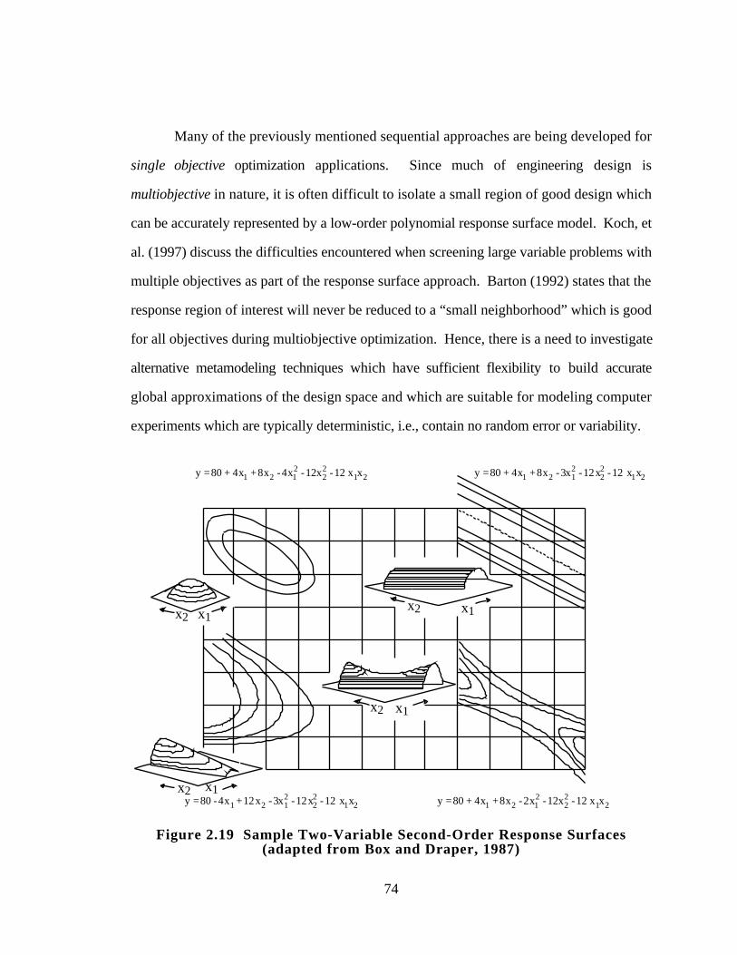
74
Many of the previously mentioned sequential approaches are being developed for
single objective optimization applications. Since much of engineering design is
multiobjective in nature, it is often difficult to isolate a small region of good design which
can be accurately represented by a low-order polynomial response surface model. Koch, et
al. (1997) discuss the difficulties encountered when screening large variable problems with
multiple objectives as part of the response surface approach. Barton (1992) states that the
response region of interest will never be reduced to a “small neighborhood” which is good
for all objectives during multiobjective optimization. Hence, there is a need to investigate
alternative metamodeling techniques which have sufficient flexibility to build accurate
global approximations of the design space and which are suitable for modeling computer
experiments which are typically deterministic, i.e., contain no random error or variability.
y x=80 -4x +12x -3x -12x -12 x1 2 12
22
1 2 y x=80 + 4x +8x -2x -12x -12 x1 2 12
22
1 2
y x=80 + 4x +8x -4x -12x -12 x1 2 12
22
1 2 y x=80 + 4x +8x -3x -12x -12 x1 2 12
22
1 2
x2 x1
x1
x1
x1
x2
x2
x2
Figure 2.19 Sample Two-Variable Second-Order Response Surfaces(adapted from Box and Draper, 1987)
75
The approach investigated in this dissertation is called kriging, and it is introduced
in the next section. This discussion of kriging is followed by a discussion of different
experimental designs which can be used to sample the design space in Section 2.4.3.
These two sections lay the foundation for the work in Chapters 4 and 5 wherein
Hypotheses 2 and 3 are tested explicitly to determine the utility of kriging and space filling
experimental designs for building approximations of deterministic computer experiments.
2 .4 .2 The Kriging Approach to Metamodeling
Kriging has its roots in the field of geostatistics—a hybrid discipline of mining
engineering, geology, mathematics, and statistics (cf., Cressie, 1993)—and is useful for
predicting temporally and spatially correlated data. Kriging is named after D. G. Krige, a
South African mining engineer who, in the 1950s, developed empirical methods for
determining true ore grade distributions from distributions based on sampled ore grades
(Matheron, 1963). Several texts which describe kriging and its usefulness for predicting
spatially correlated data (see, e.g., Cressie, 1993) and mining (see, e.g., Journel and
Huijbregts, 1978) exist. These metamodels are extremely flexible due to the wide range of
correlation functions which can be chosen for building the metamodel. Furthermore,
depending on the choice of the correlation function, the metamodel can either “honor the
data,” providing an exact interpolation of the data, or “smooth the data,” providing an
inexact interpolation (Cressie, 1993). In this work, as in most applications of kriging, the
concern is solely on spatial prediction; it is assumed that the data are not correlated
temporally.
These days, kriging goes by a variety of names including DACE (Design and
Analysis of Computer Experiments) modeling—the title of the inaugural paper by Sacks, et
al. (1989)—and spatial correlation metamodeling (see, e.g., Barton, 1994). There are also
several types of kriging (cf., Cressie, 1993): ordinary kriging, universal kriging,
76
lognormal kriging, and trans-Gaussian kriging. In this dissertation, ordinary kriging is
employed, following the work in, e.g., (Booker, et al., 1995; Koehler and Owen, 1996),
and only the term kriging is used.
Unlike response surfaces, however, kriging models have found limited use in
engineering design applications since introduction into the literature by Sacks, et al. (1989).
Consequently, the following question is addressed in this dissertation:
Q2. Is kriging a viable metamodeling technique for building approximations of
deterministic computer analyses?
As introduced in Section 1.3.1, Hypothesis 2 is that kriging is a viable
metamodeling technique for building approximations of deterministic
computer analyses. Initial applications of kriging in engineering design include:
• Giunta (1997) and Giunta, et al. (1998) perform a preliminary investigation into the
use of kriging for the multidisciplinary design optimization of a High Speed Civil
Transport aircraft.
• Sasena (1998) compares and contrasts kriging and smoothing splines for
approximating noisy data.
• Schonlau, et al. (1997) use a global/local search algorithm based on kriging for
shape optimization of an automobile piston engine.
• Osio and Amon (1996) develop a multistage numerical optimization strategy based
on kriging which they demonstrate on the thermal design of embedded electronic
package which has 5 design variables.
• Booker (1996) and Booker, et al. (1996) using a kriging approach to study the
aeroelastic and dynamic response of a helicopter rotor during structural design.
77
Some researchers have also employed kriging-based strategies for numerical optimization
(see, e.g., Cox and John, 1995; Trosset and Torczon, 1997). A look at the mathematics of
kriging is offered next.
Mathematics of Kriging
Kriging postulates a combination of a polynomial model and departures of the following
form:
y(x) = f(x) + Z(x) [2.18]
where y(x) is the unknown function of interest, f(x) is a known polynomial function of x ,
and Z(x) is the realization of a stochastic process with mean zero, variance σ2, and non-
zero covariance. The f(x) term in Equation 2.18 is similar to the polynomial model in a
response surface, providing a “global” model of the design space. In many cases f(x) is
simply taken to be a constant term β (cf., Koehler and Owen, 1996; Sacks, et al., 1989;
Welch, et al., 1990). Only kriging models with constant underlying global models are
investigated in this work as well.
While f(x) “globally” approximates the design space, Z(x) creates “localized”
deviations so that the kriging model interpolates the ns sampled data points. The covariance
matrix of Z(x) which dictates the local deviations is as follows:
Cov[Z(x i),Z(x j)] = σ2 R([R(x i,x j)] [2.19]
where R is the correlation matrix, and R(x i,x j) is the correlation function between any two
of the ns sampled data points x i and x j. R is a ns x ns symmetric, positive definite matrix
with ones along the diagonal. The correlation function R(x i,x j) is specified by the user.
In this work, five different correlation functions are examined for use in the kriging
model, see Table 2.1. In all of the correlation functions listed in Table 2.1, ndv is the
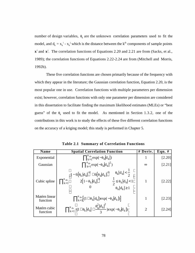
78
number of design variables, θk are the unknown correlation parameters used to fit the
model, and dk = xki - xk
j which is the distance between the kth components of sample points
x i and x j. The correlation functions of Equations 2.20 and 2.21 are from (Sacks, et al.,
1989); the correlation functions of Equations 2.22-2.24 are from (Mitchell and Morris,
1992b).
These five correlation functions are chosen primarily because of the frequency with
which they appear in the literature; the Gaussian correlation function, Equation 2.20, is the
most popular one in use. Correlation functions with multiple parameters per dimension
exist; however, correlation functions with only one parameter per dimension are considered
in this dissertation to facilitate finding the maximum likelihood estimates (MLEs) or “best
guess” of the θk used to fit the model. As mentioned in Section 1.3.2, one of the
contributions in this work is to study the effects of these five different correlation functions
on the accuracy of a kriging model; this study is performed in Chapter 5.
Table 2.1 Summary of Correlation Functions
Name Spatial Correlation Function # Deriv. Eqn. #
Exponential exp(−θk dk )k=1
n dv∏ 1 [2.20]
Gaussian exp(−θk dk2)k=1
ndv∏ ∞ [2.21]
Cubic spline
1 − 6 θk dk( )2+ 6 θk dk( )3
2 1− θk dk( )3
0
θk dk <1
21
2≤ θk dk <1
θk dk ≥1
k=1
n dv∏ 1 [2.22]
Matérn linearfunction (1+ θk dk )exp( −θk dk )[ ]k=1
n dv∏ 1 [2.23]
Matérn cubicfunction
(1+ θk dk +θk
2 dk2
3)exp( −θk dk )
k=1
n dv∏ 2 [2.24]
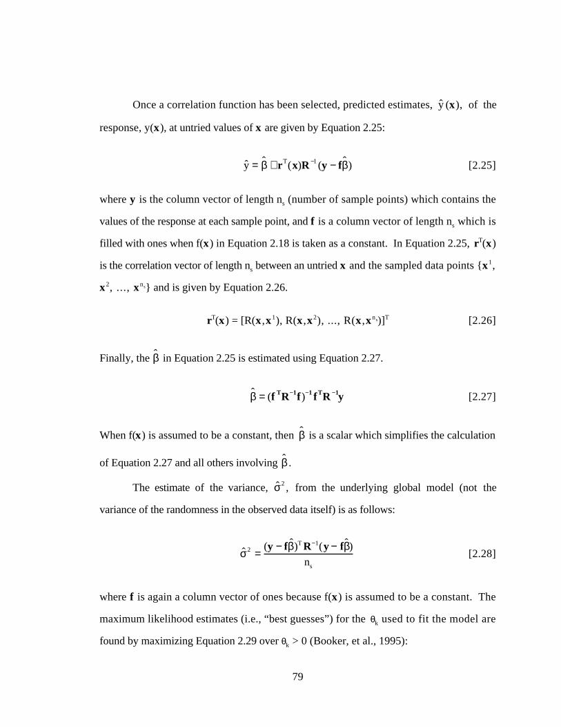
79
Once a correlation function has been selected, predicted estimates, ˆ y (x), of the
response, y(x), at untried values of x are given by Equation 2.25:
ˆ y = ˆ β + rT(x)R −1 (y − fˆ β ) [2.25]
where y is the column vector of length ns (number of sample points) which contains the
values of the response at each sample point, and f is a column vector of length ns which is
filled with ones when f(x) in Equation 2.18 is taken as a constant. In Equation 2.25, rT(x)
is the correlation vector of length ns between an untried x and the sampled data points {x1,
x2, ..., xns} and is given by Equation 2.26.
rT(x) = [R(x ,x1), R(x ,x2), ..., R(x ,xns)]T [2.26]
Finally, the ˆ β in Equation 2.25 is estimated using Equation 2.27.
ˆ β = (f TR−1f)−1 fTR −1y [2.27]
When f(x) is assumed to be a constant, then ˆ β is a scalar which simplifies the calculation
of Equation 2.27 and all others involving ˆ β .
The estimate of the variance, ˆ σ 2 , from the underlying global model (not the
variance of the randomness in the observed data itself) is as follows:
ˆ σ 2 =(y − f ˆ β )T R−1(y − fˆ β )
ns
[2.28]
where f is again a column vector of ones because f(x) is assumed to be a constant. The
maximum likelihood estimates (i.e., “best guesses”) for the θk used to fit the model are
found by maximizing Equation 2.29 over θk > 0 (Booker, et al., 1995):
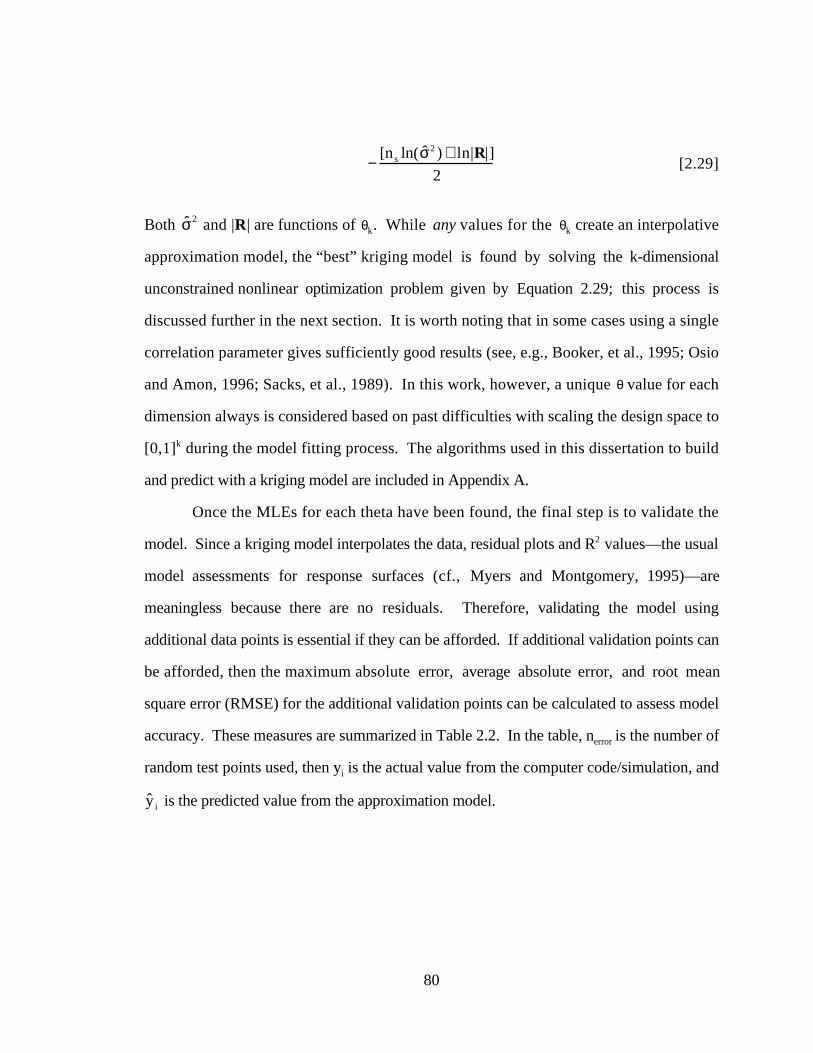
80
−[n s ln( ˆ σ 2 ) + ln|R|]
2[2.29]
Both ˆ σ 2 and |R| are functions of θk. While any values for the θk create an interpolative
approximation model, the “best” kriging model is found by solving the k-dimensional
unconstrained nonlinear optimization problem given by Equation 2.29; this process is
discussed further in the next section. It is worth noting that in some cases using a single
correlation parameter gives sufficiently good results (see, e.g., Booker, et al., 1995; Osio
and Amon, 1996; Sacks, et al., 1989). In this work, however, a unique θ value for each
dimension always is considered based on past difficulties with scaling the design space to
[0,1]k during the model fitting process. The algorithms used in this dissertation to build
and predict with a kriging model are included in Appendix A.
Once the MLEs for each theta have been found, the final step is to validate the
model. Since a kriging model interpolates the data, residual plots and R2 values—the usual
model assessments for response surfaces (cf., Myers and Montgomery, 1995)—are
meaningless because there are no residuals. Therefore, validating the model using
additional data points is essential if they can be afforded. If additional validation points can
be afforded, then the maximum absolute error, average absolute error, and root mean
square error (RMSE) for the additional validation points can be calculated to assess model
accuracy. These measures are summarized in Table 2.2. In the table, nerror is the number of
random test points used, then yi is the actual value from the computer code/simulation, and
ˆ y i is the predicted value from the approximation model.
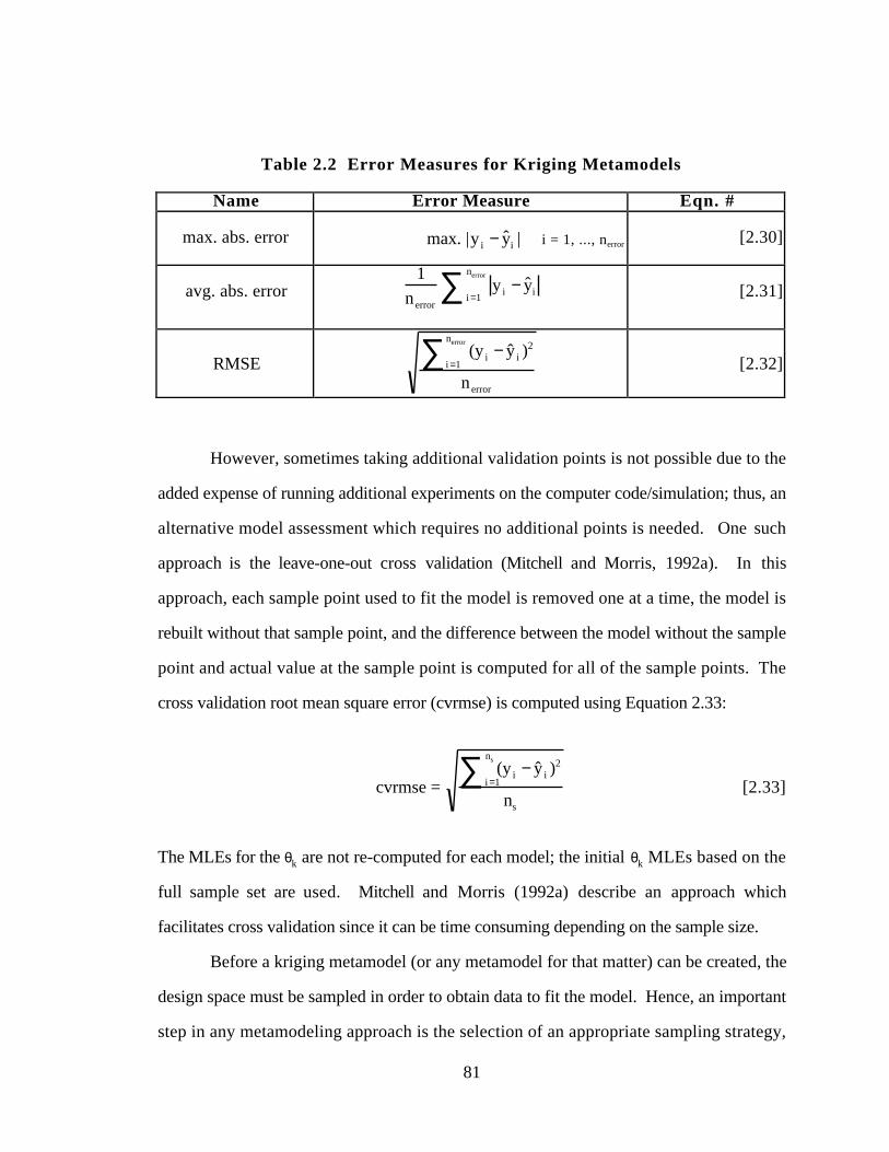
81
Table 2.2 Error Measures for Kriging Metamodels
Name Error Measure Eqn. #
max. abs. error max. |y i − ˆ y i | i = 1, ..., nerror [2.30]
avg. abs. error1
n error
y i − ˆ y ii =1
nerror∑ [2.31]
RMSE(y i − ˆ y i )
2
i =1
nerror∑n error
[2.32]
However, sometimes taking additional validation points is not possible due to the
added expense of running additional experiments on the computer code/simulation; thus, an
alternative model assessment which requires no additional points is needed. One such
approach is the leave-one-out cross validation (Mitchell and Morris, 1992a). In this
approach, each sample point used to fit the model is removed one at a time, the model is
rebuilt without that sample point, and the difference between the model without the sample
point and actual value at the sample point is computed for all of the sample points. The
cross validation root mean square error (cvrmse) is computed using Equation 2.33:
cvrmse = (y i − ˆ y i )
2
i =1
ns∑ns
[2.33]
The MLEs for the θk are not re-computed for each model; the initial θk MLEs based on the
full sample set are used. Mitchell and Morris (1992a) describe an approach which
facilitates cross validation since it can be time consuming depending on the sample size.
Before a kriging metamodel (or any metamodel for that matter) can be created, the
design space must be sampled in order to obtain data to fit the model. Hence, an important
step in any metamodeling approach is the selection of an appropriate sampling strategy,
82
i.e., an experimental design by which the computer analysis or simulation code is queried.
In the next section, space filling and classical experimental designs are discussed.
2 .4 .3 Classical and Space Filling Experimental Designs
Many researchers (see, e.g., Currin, et al., 1991; Sacks and Schiller, 1988) argue
that classical experimental designs, such as the central composite designs and Box-
Behnken designs, are not well-suited for sampling deterministic computer experiments.
Sacks, et al. (1989) state that the “classical notions of experimental blocking, replication
and randomization are irrelevant” when it comes to deterministic computer experiments that
have no random error; hence, designs for deterministic computer experiments should “fill
the space” as opposed to possess properties for estimating the variability in the data.
Booker (1996) summarizes the difference between classical experimental designs
and new space filling designs well. In the classical design and analysis of physical
experiments, random variation is accounted for by spreading the sample points out in the
design space and by taking multiple data points (replicates), see Figure 2.20a. In
deterministic computer experiments, replication at a sample point is meaningless; therefore,
the points should be chosen to fill the design space. One approach is to minimize the
integrated mean square error over the design region (cf., Sacks, et al., 1989); the space
filling design illustrated in Figure 2.20b is an example of such a design.
As part of the research in this dissertation, the following question is addressed.
Q3. Are space filling designs better suited for building approximations of
deterministic computer analyses than classical experimental designs?
As stated in Section 1.3.1, Hypothesis 3 is that space filling designs are
better suited for building approximations of deterministic computer
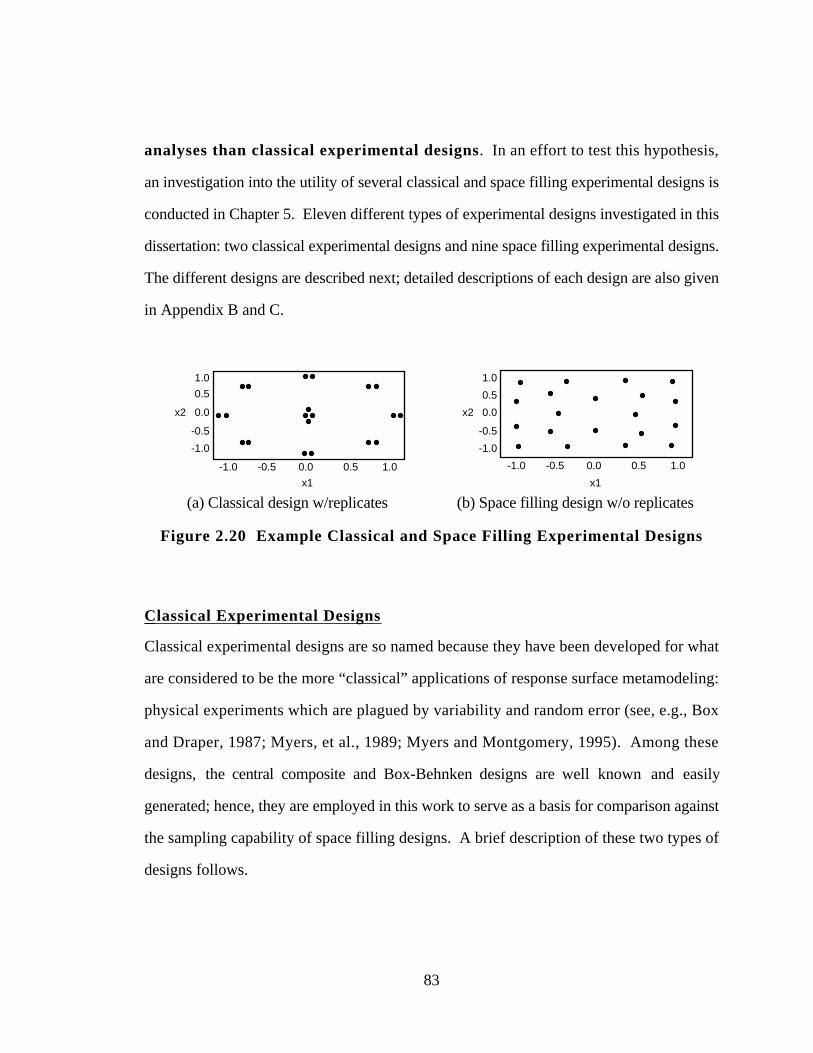
83
analyses than classical experimental designs. In an effort to test this hypothesis,
an investigation into the utility of several classical and space filling experimental designs is
conducted in Chapter 5. Eleven different types of experimental designs investigated in this
dissertation: two classical experimental designs and nine space filling experimental designs.
The different designs are described next; detailed descriptions of each design are also given
in Appendix B and C.
0.0x2
0.5
1.0
-0.5
-1.0
x1
0.0 0.5-0.5-1.0 1.0
0.0x2
x1
0.0
0.5
1.0
-0.5
-1.0
0.5-0.5-1.0 1.0
(a) Classical design w/replicates (b) Space filling design w/o replicates
Figure 2.20 Example Classical and Space Filling Experimental Designs
Classical Experimental Designs
Classical experimental designs are so named because they have been developed for what
are considered to be the more “classical” applications of response surface metamodeling:
physical experiments which are plagued by variability and random error (see, e.g., Box
and Draper, 1987; Myers, et al., 1989; Myers and Montgomery, 1995). Among these
designs, the central composite and Box-Behnken designs are well known and easily
generated; hence, they are employed in this work to serve as a basis for comparison against
the sampling capability of space filling designs. A brief description of these two types of
designs follows.
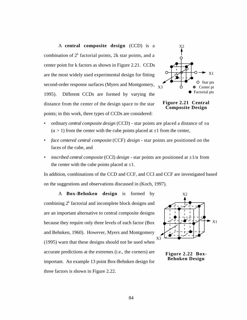
84
A central composite design (CCD) is a
combination of 2k factorial points, 2k star points, and a
center point for k factors as shown in Figure 2.21. CCDs
are the most widely used experimental design for fitting
second-order response surfaces (Myers and Montgomery,
1995). Different CCDs are formed by varying the
distance from the center of the design space to the star
points; in this work, three types of CCDs are considered:
X1
X2
X3Star pts
Center ptFactorial pts
Figure 2.21 CentralComposite Design
• ordinary central composite design (CCD) - star points are placed a distance of ±α
(α > 1) from the center with the cube points placed at ±1 from the center,
• face centered central composite (CCF) design - star points are positioned on the
faces of the cube, and
• inscribed central composite (CCI) design - star points are positioned at ±1/α from
the center with the cube points placed at ±1.
In addition, combinations of the CCD and CCF, and CCI and CCF are investigated based
on the suggestions and observations discussed in (Koch, 1997).
A Box-Behnken design is formed by
combining 2k factorial and incomplete block designs and
are an important alternative to central composite designs
because they require only three levels of each factor (Box
and Behnken, 1960). However, Myers and Montgomery
(1995) warn that these designs should not be used when
accurate predictions at the extremes (i.e., the corners) are
important. An example 13 point Box-Behnken design for
three factors is shown in Figure 2.22.
X1
X2
X3
Figure 2.22 Box-Behnken Design
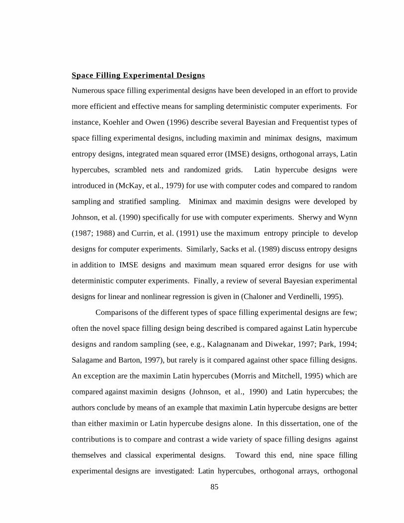
85
Space Filling Experimental Designs
Numerous space filling experimental designs have been developed in an effort to provide
more efficient and effective means for sampling deterministic computer experiments. For
instance, Koehler and Owen (1996) describe several Bayesian and Frequentist types of
space filling experimental designs, including maximin and minimax designs, maximum
entropy designs, integrated mean squared error (IMSE) designs, orthogonal arrays, Latin
hypercubes, scrambled nets and randomized grids. Latin hypercube designs were
introduced in (McKay, et al., 1979) for use with computer codes and compared to random
sampling and stratified sampling. Minimax and maximin designs were developed by
Johnson, et al. (1990) specifically for use with computer experiments. Sherwy and Wynn
(1987; 1988) and Currin, et al. (1991) use the maximum entropy principle to develop
designs for computer experiments. Similarly, Sacks et al. (1989) discuss entropy designs
in addition to IMSE designs and maximum mean squared error designs for use with
deterministic computer experiments. Finally, a review of several Bayesian experimental
designs for linear and nonlinear regression is given in (Chaloner and Verdinelli, 1995).
Comparisons of the different types of space filling experimental designs are few;
often the novel space filling design being described is compared against Latin hypercube
designs and random sampling (see, e.g., Kalagnanam and Diwekar, 1997; Park, 1994;
Salagame and Barton, 1997), but rarely is it compared against other space filling designs.
An exception are the maximin Latin hypercubes (Morris and Mitchell, 1995) which are
compared against maximin designs (Johnson, et al., 1990) and Latin hypercubes; the
authors conclude by means of an example that maximin Latin hypercube designs are better
than either maximin or Latin hypercube designs alone. In this dissertation, one of the
contributions is to compare and contrast a wide variety of space filling designs against
themselves and classical experimental designs. Toward this end, nine space filling
experimental designs are investigated: Latin hypercubes, orthogonal arrays, orthogonal
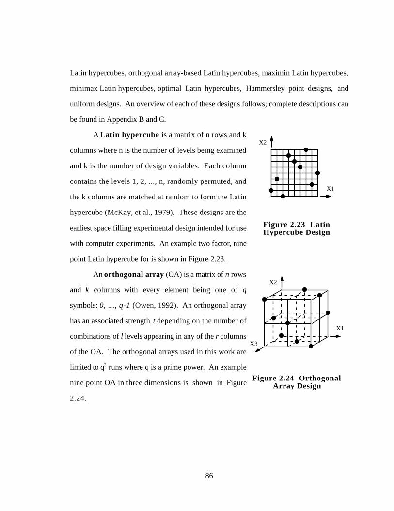
86
Latin hypercubes, orthogonal array-based Latin hypercubes, maximin Latin hypercubes,
minimax Latin hypercubes, optimal Latin hypercubes, Hammersley point designs, and
uniform designs. An overview of each of these designs follows; complete descriptions can
be found in Appendix B and C.
A Latin hypercube is a matrix of n rows and k
columns where n is the number of levels being examined
and k is the number of design variables. Each column
contains the levels 1, 2, ..., n, randomly permuted, and
the k columns are matched at random to form the Latin
hypercube (McKay, et al., 1979). These designs are the
earliest space filling experimental design intended for use
with computer experiments. An example two factor, nine
point Latin hypercube for is shown in Figure 2.23.
X1
X2
Figure 2.23 LatinHypercube Design
An orthogonal array (OA) is a matrix of n rows
and k columns with every element being one of q
symbols: 0, ..., q-1 (Owen, 1992). An orthogonal array
has an associated strength t depending on the number of
combinations of l levels appearing in any of the r columns
of the OA. The orthogonal arrays used in this work are
limited to q2 runs where q is a prime power. An example
nine point OA in three dimensions is shown in Figure
2.24.
X1
X2
X3
Figure 2.24 OrthogonalArray Design
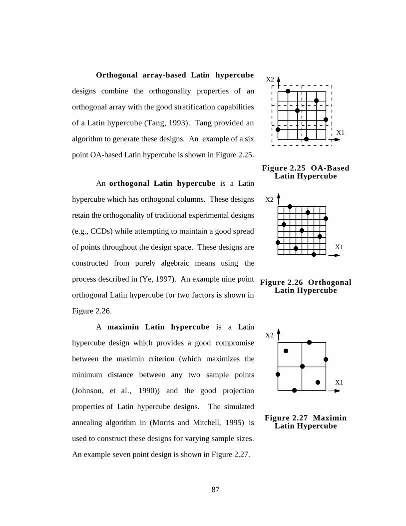
87
Orthogonal array-based Latin hypercube
designs combine the orthogonality properties of an
orthogonal array with the good stratification capabilities
of a Latin hypercube (Tang, 1993). Tang provided an
algorithm to generate these designs. An example of a six
point OA-based Latin hypercube is shown in Figure 2.25.
X1
X2
Figure 2.25 OA-BasedLatin Hypercube
An orthogonal Latin hypercube is a Latin
hypercube which has orthogonal columns. These designs
retain the orthogonality of traditional experimental designs
(e.g., CCDs) while attempting to maintain a good spread
of points throughout the design space. These designs are
constructed from purely algebraic means using the
process described in (Ye, 1997). An example nine point
orthogonal Latin hypercube for two factors is shown in
Figure 2.26.
X1
X2
Figure 2.26 OrthogonalLatin Hypercube
A maximin Latin hypercube is a Latin
hypercube design which provides a good compromise
between the maximin criterion (which maximizes the
minimum distance between any two sample points
(Johnson, et al., 1990)) and the good projection
properties of Latin hypercube designs. The simulated
annealing algorithm in (Morris and Mitchell, 1995) is
used to construct these designs for varying sample sizes.
An example seven point design is shown in Figure 2.27.
X1
X2
Figure 2.27 MaximinLatin Hypercube
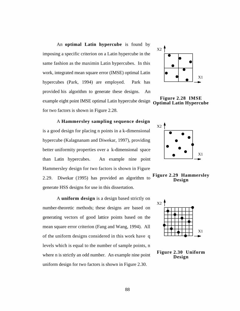
88
An optimal Latin hypercube is found by
imposing a specific criterion on a Latin hypercube in the
same fashion as the maximin Latin hypercubes. In this
work, integrated mean square error (IMSE) optimal Latin
hypercubes (Park, 1994) are employed. Park has
provided his algorithm to generate these designs. An
example eight point IMSE optimal Latin hypercube design
for two factors is shown in Figure 2.28.
X1
X2
Figure 2.28 IMSEOptimal Latin Hypercube
A Hammersley sampling sequence design
is a good design for placing n points in a k-dimensional
hypercube (Kalagnanam and Diwekar, 1997), providing
better uniformity properties over a k-dimensional space
than Latin hypercubes. An example nine point
Hammersley design for two factors is shown in Figure
2.29. Diwekar (1995) has provided an algorithm to
generate HSS designs for use in this dissertation.
X1
X2
Figure 2.29 HammersleyDesign
A uniform design is a design based strictly on
number-theoretic methods; these designs are based on
generating vectors of good lattice points based on the
mean square error criterion (Fang and Wang, 1994). All
of the uniform designs considered in this work have q
levels which is equal to the number of sample points, n
where n is strictly an odd number. An example nine point
uniform design for two factors is shown in Figure 2.30.
X1
X2
Figure 2.30 UniformDesign
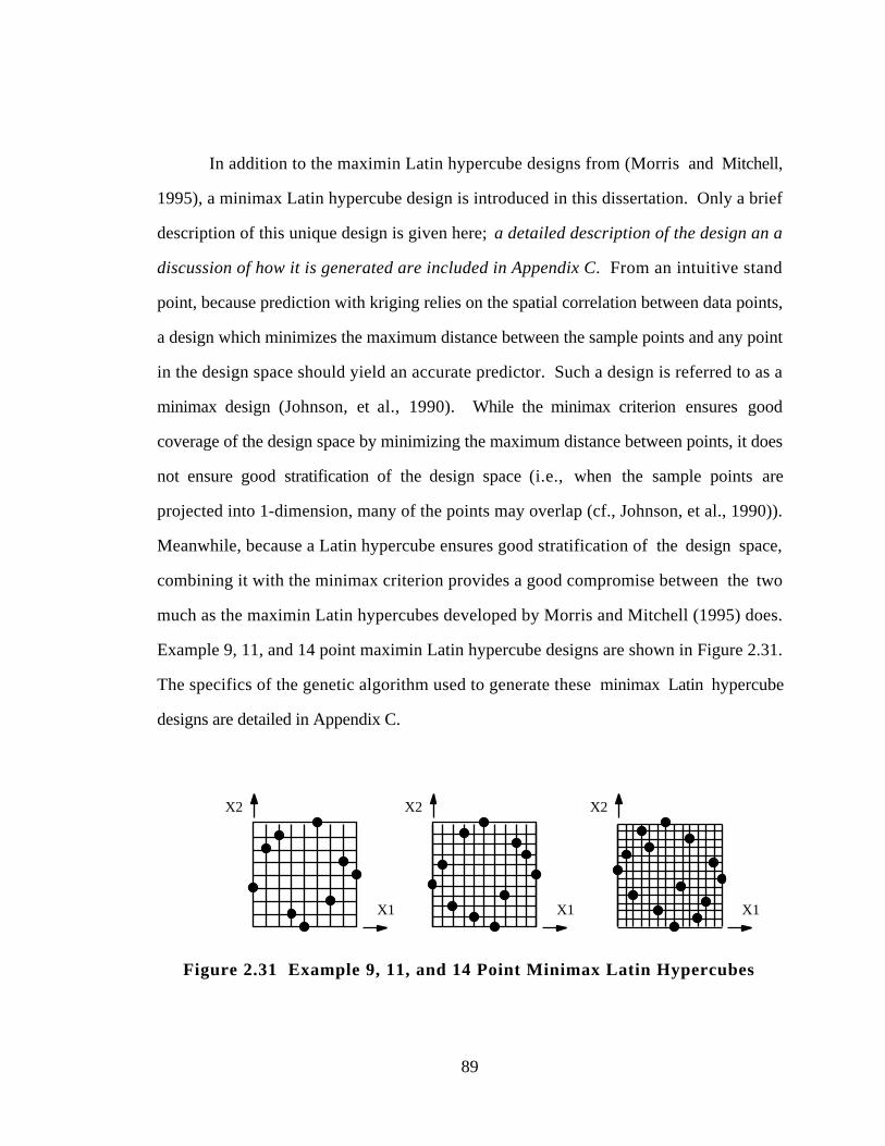
89
In addition to the maximin Latin hypercube designs from (Morris and Mitchell,
1995), a minimax Latin hypercube design is introduced in this dissertation. Only a brief
description of this unique design is given here; a detailed description of the design an a
discussion of how it is generated are included in Appendix C. From an intuitive stand
point, because prediction with kriging relies on the spatial correlation between data points,
a design which minimizes the maximum distance between the sample points and any point
in the design space should yield an accurate predictor. Such a design is referred to as a
minimax design (Johnson, et al., 1990). While the minimax criterion ensures good
coverage of the design space by minimizing the maximum distance between points, it does
not ensure good stratification of the design space (i.e., when the sample points are
projected into 1-dimension, many of the points may overlap (cf., Johnson, et al., 1990)).
Meanwhile, because a Latin hypercube ensures good stratification of the design space,
combining it with the minimax criterion provides a good compromise between the two
much as the maximin Latin hypercubes developed by Morris and Mitchell (1995) does.
Example 9, 11, and 14 point maximin Latin hypercube designs are shown in Figure 2.31.
The specifics of the genetic algorithm used to generate these minimax Latin hypercube
designs are detailed in Appendix C.
X1
X2
X1
X2
X1
X2
Figure 2.31 Example 9, 11, and 14 Point Minimax Latin Hypercubes
90
In Chapter 5, the minimax Latin hypercube designs are compared against the other
classical and space filling experimental designs discussed in this section. A look ahead to
that and the next chapters is offered in the next section.
2.5 A LOOK BACK AND A LOOK AHEAD
Through the review of the literature which is presented in this chapter, the
necessary elements for a method to model and design a scalable product platform for a
product family have been identified by elucidating the research questions (and hypotheses)
introduced in Section 1.3.1. In the next chapter, these constitutive elements are integrated
to create the Product Platform Concept Exploration Method (PPCEM), providing a Method
which facilitates the synthesis and Exploration of a common Product Platform Concept
which can be scaled into an appropriate family of products. The relationship between the
individual sections in this chapter and the PPCEM developed in the next chapter are
illustrated in Figure 2.32. In particular, the market segmentation grid is revisited in Section
3.1.1 as it applies to the PPCEM. The concept of a “conceptual noise factor” is formalized
into a scale factor in Section 3.1.2 which is fundamental to the utilization of the PPCEM.
Metamodeling techniques within the PPCEM are discussed in Sections 3.1.3. Aggregation
of the individual product specifications into an appropriate comproimse DSP formulation
for the product family is described in Section 3.1.4, and development of the product
platform portfolio for the product family is explained in Section 3.1.5.
In addition to the presentation of the PPCEM, the research hypotheses are revisited
in Section 3.2 in the next chapter. Supporting posits are stated for each hypothesis, and the
verification strategy for testing the hypotheses is elaborated in Section 3.3. The discussion
in Section 3.3 sets the stage for the example problems which are presented in Chapters 4
through 7 to verify the hypotheses.
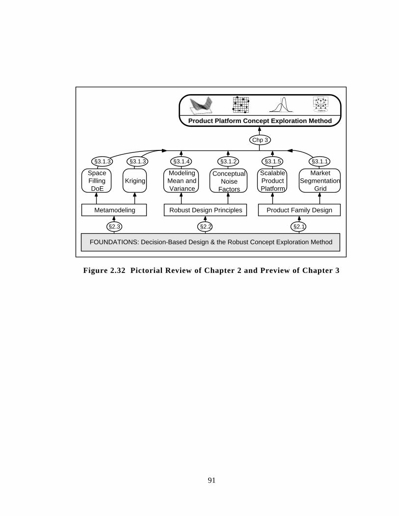
91
Metamodeling
ModelingMean andVariance
Robust Design Principles
ConceptualNoise
Factors
ScalableProductPlatform
MarketSegmentation
Grid
Product Family Design
KrigingSpaceFillingDoE
Chp 3
§2.2§2.3 §2.1
FOUNDATIONS: Decision-Based Design & the Robust Concept Exploration Method
Platform
Product Platform Concept Exploration Method
§3.1.5 §3.1.1§3.1.2§3.1.4§3.1.3§3.1.3
Figure 2.32 Pictorial Review of Chapter 2 and Preview of Chapter 3

92
3. CHAPTER 3
THE PRODUCT PLATFORM CONCEPTEXPLORATION METHOD
Platform
Product Platform Concept Exploration Method
In this chapter, the elements of the previous chapters are synthesized to meet the
principal objective in this dissertation, namely, to develop the Product Platform Concept
Exploration Method (PPCEM) for designing a common scalable product platform for a
product family. An overview of the PPCEM and its associated steps and tools is given in
Section 3.1 with each step of the PPCEM and its constituent elements elaborated in
Sections 3.1.1 through 3.1.5; the resulting infrastructure of the PPCEM is presented in
Section 3.1.6. In Section 3.2, the research hypotheses are revisited from Section 1.3.1
and supporting posits are identified. Section 3.3 follows with an outline of the strategy for
verification and testing of the research hypotheses. Section 3.4 concludes the chapter with
a recap of what has been presented and a look ahead to the metamodeling studies in
Chapters 4 and 5 and the example problems in Chapters 6 and 7 which are used to test the
research hypotheses and demonstrate the application of the PPCEM.
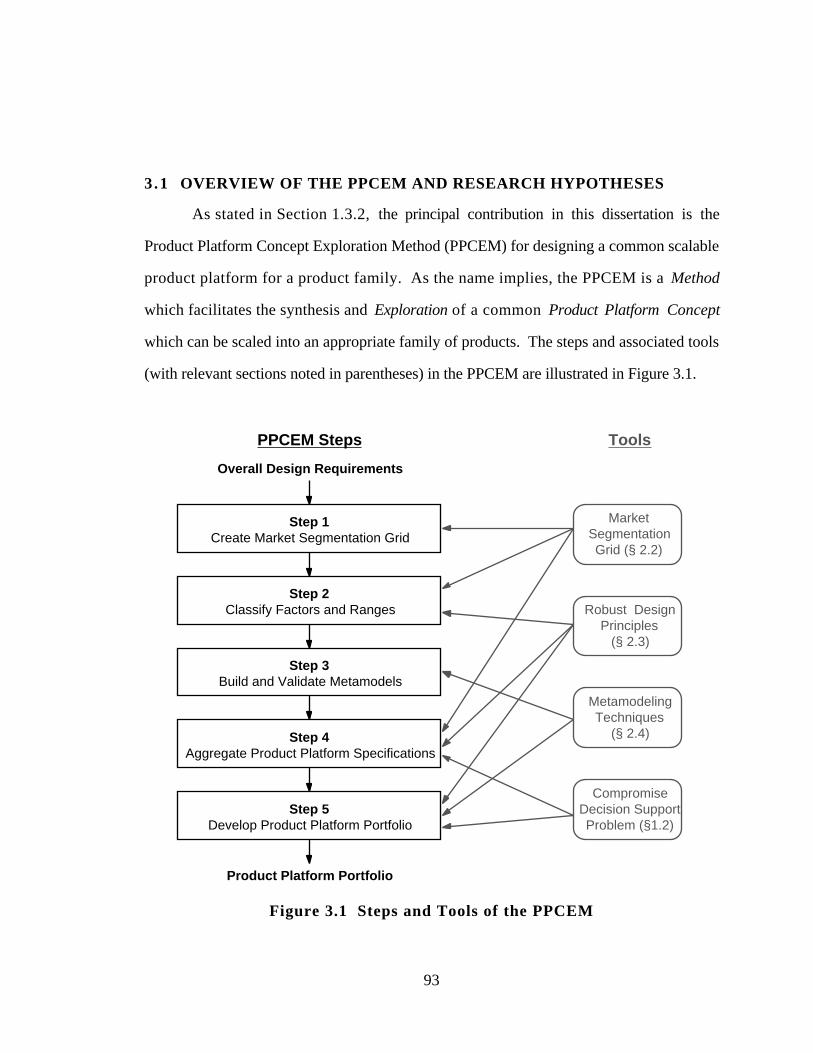
93
3.1 OVERVIEW OF THE PPCEM AND RESEARCH HYPOTHESES
As stated in Section 1.3.2, the principal contribution in this dissertation is the
Product Platform Concept Exploration Method (PPCEM) for designing a common scalable
product platform for a product family. As the name implies, the PPCEM is a Method
which facilitates the synthesis and Exploration of a common Product Platform Concept
which can be scaled into an appropriate family of products. The steps and associated tools
(with relevant sections noted in parentheses) in the PPCEM are illustrated in Figure 3.1.
Tools
Market Segmentation Grid (§ 2.2)
Robust Design Principles
(§ 2.3)
Metamodeling Techniques
(§ 2.4)
Compromise Decision Support Problem (§1.2)
Step 1Create Market Segmentation Grid
Step 2Classify Factors and Ranges
Step 3Build and Validate Metamodels
Step 4Aggregate Product Platform Specifications
Step 5Develop Product Platform Portfolio
PPCEM Steps
Overall Design Requirements
Product Platform Portfolio
Figure 3.1 Steps and Tools of the PPCEM
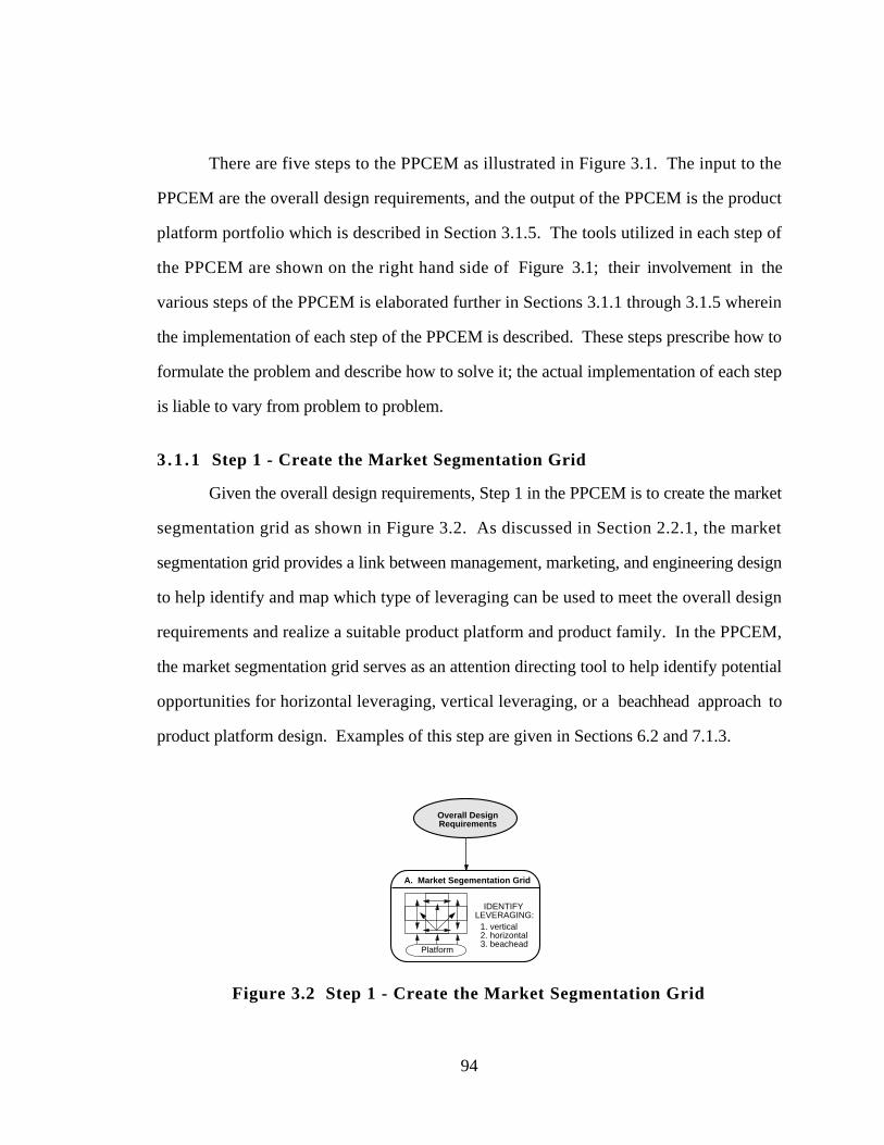
94
There are five steps to the PPCEM as illustrated in Figure 3.1. The input to the
PPCEM are the overall design requirements, and the output of the PPCEM is the product
platform portfolio which is described in Section 3.1.5. The tools utilized in each step of
the PPCEM are shown on the right hand side of Figure 3.1; their involvement in the
various steps of the PPCEM is elaborated further in Sections 3.1.1 through 3.1.5 wherein
the implementation of each step of the PPCEM is described. These steps prescribe how to
formulate the problem and describe how to solve it; the actual implementation of each step
is liable to vary from problem to problem.
3 .1 .1 Step 1 - Create the Market Segmentation Grid
Given the overall design requirements, Step 1 in the PPCEM is to create the market
segmentation grid as shown in Figure 3.2. As discussed in Section 2.2.1, the market
segmentation grid provides a link between management, marketing, and engineering design
to help identify and map which type of leveraging can be used to meet the overall design
requirements and realize a suitable product platform and product family. In the PPCEM,
the market segmentation grid serves as an attention directing tool to help identify potential
opportunities for horizontal leveraging, vertical leveraging, or a beachhead approach to
product platform design. Examples of this step are given in Sections 6.2 and 7.1.3.
A. Market Segementation Grid
IDENTIFYLEVERAGING:
1. vertical 2. horizontal 3. beachead
Overall Design Requirements
Platform
Figure 3.2 Step 1 - Create the Market Segmentation Grid
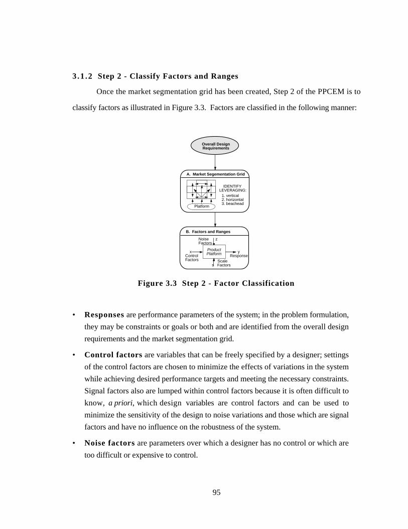
95
3 .1 .2 Step 2 - Classify Factors and Ranges
Once the market segmentation grid has been created, Step 2 of the PPCEM is to
classify factors as illustrated in Figure 3.3. Factors are classified in the following manner:
yResponse
Noise zFactors
xControlFactors Scale
s Factors
B. Factors and Ranges
Overall Design Requirements
ProductPlatform
A. Market Segementation Grid
IDENTIFYLEVERAGING:
1. vertical 2. horizontal 3. beachead
Platform
Figure 3.3 Step 2 - Factor Classification
• Responses are performance parameters of the system; in the problem formulation,
they may be constraints or goals or both and are identified from the overall design
requirements and the market segmentation grid.
• Control factors are variables that can be freely specified by a designer; settings
of the control factors are chosen to minimize the effects of variations in the system
while achieving desired performance targets and meeting the necessary constraints.
Signal factors also are lumped within control factors because it is often difficult to
know, a priori, which design variables are control factors and can be used to
minimize the sensitivity of the design to noise variations and those which are signal
factors and have no influence on the robustness of the system.
• Noise factors are parameters over which a designer has no control or which are
too difficult or expensive to control.
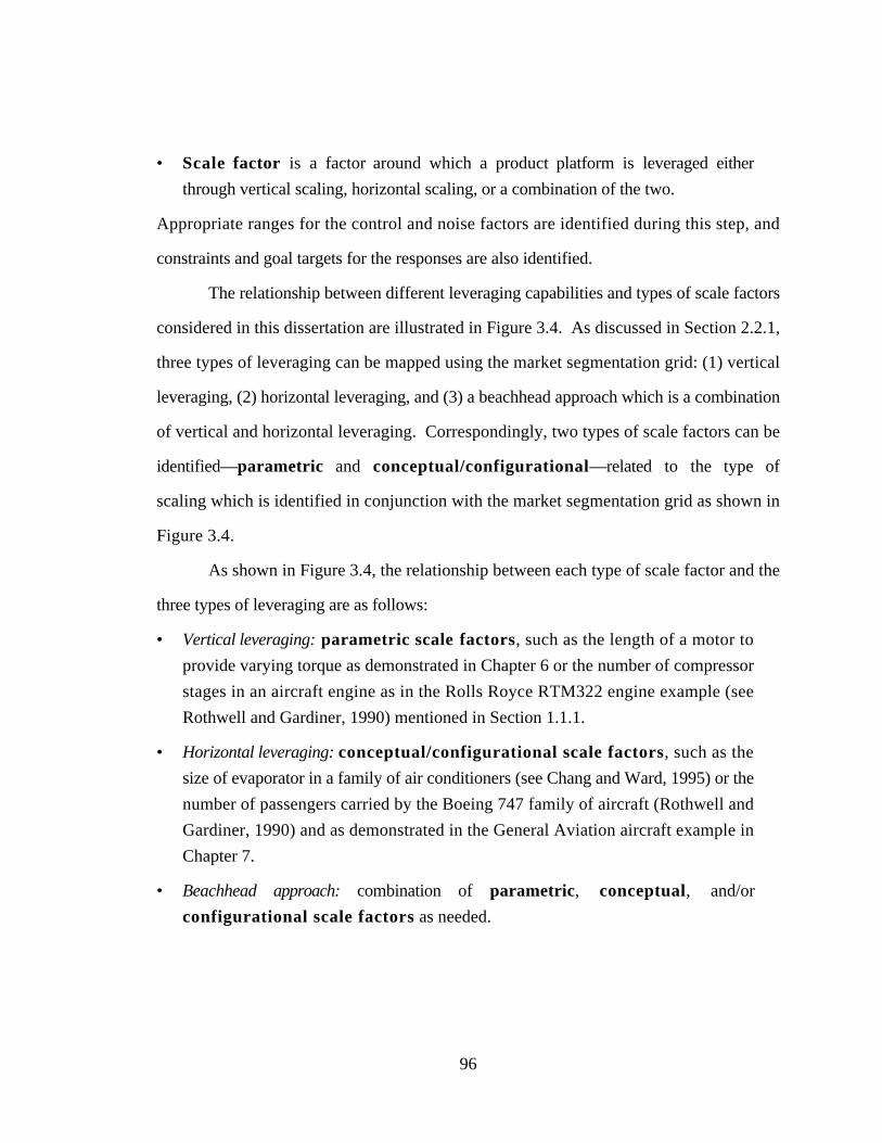
96
• Scale factor is a factor around which a product platform is leveraged either
through vertical scaling, horizontal scaling, or a combination of the two.
Appropriate ranges for the control and noise factors are identified during this step, and
constraints and goal targets for the responses are also identified.
The relationship between different leveraging capabilities and types of scale factors
considered in this dissertation are illustrated in Figure 3.4. As discussed in Section 2.2.1,
three types of leveraging can be mapped using the market segmentation grid: (1) vertical
leveraging, (2) horizontal leveraging, and (3) a beachhead approach which is a combination
of vertical and horizontal leveraging. Correspondingly, two types of scale factors can be
identified—parametric and conceptual/configurational—related to the type of
scaling which is identified in conjunction with the market segmentation grid as shown in
Figure 3.4.
As shown in Figure 3.4, the relationship between each type of scale factor and the
three types of leveraging are as follows:
• Vertical leveraging: parametric scale factors, such as the length of a motor to
provide varying torque as demonstrated in Chapter 6 or the number of compressor
stages in an aircraft engine as in the Rolls Royce RTM322 engine example (see
Rothwell and Gardiner, 1990) mentioned in Section 1.1.1.
• Horizontal leveraging: conceptual/configurational scale factors, such as the
size of evaporator in a family of air conditioners (see Chang and Ward, 1995) or the
number of passengers carried by the Boeing 747 family of aircraft (Rothwell and
Gardiner, 1990) and as demonstrated in the General Aviation aircraft example in
Chapter 7.
• Beachhead approach: combination of parametric, conceptual, and/or
configurational scale factors as needed.
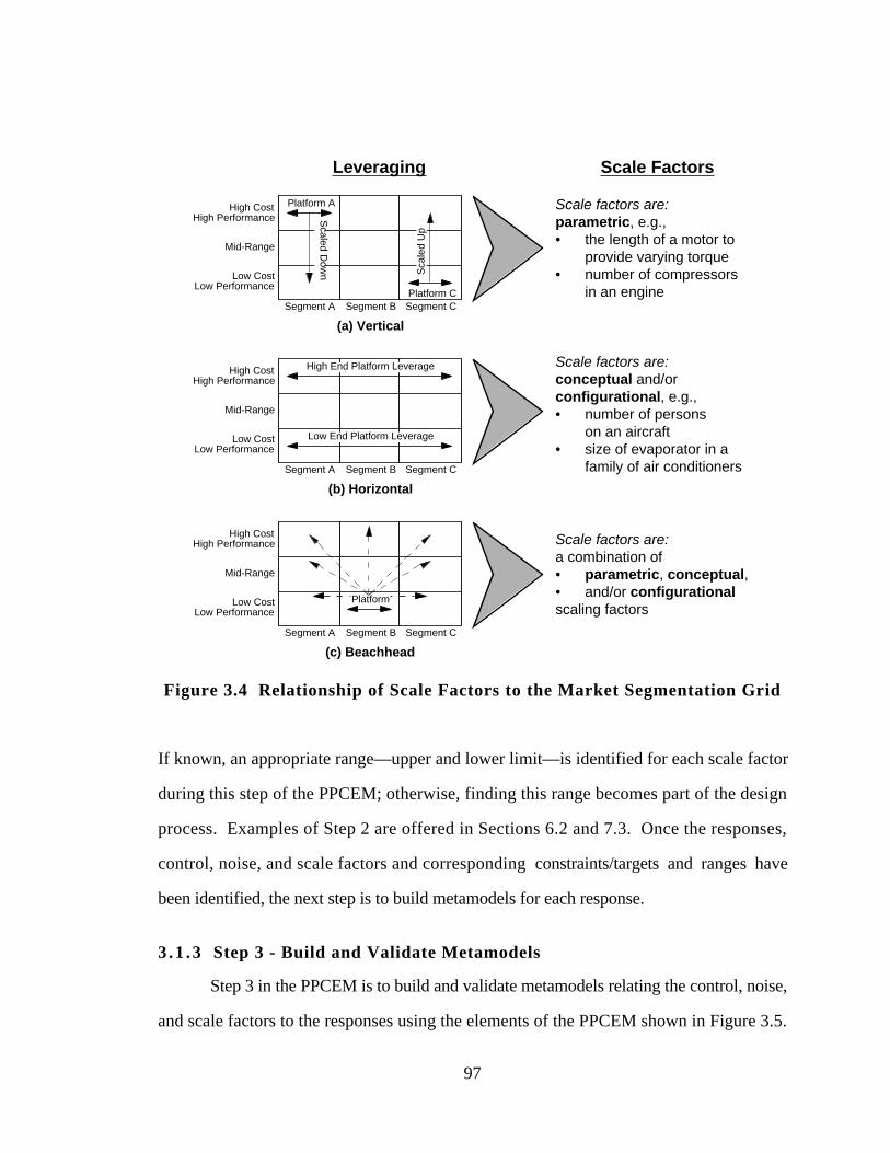
97
High CostHigh Performance
Mid-Range
Low CostLow Performance
Segment A Segment B Segment C
Platform A
Platform C
Scaled D
own S
cale
d U
p
(a) Vertical
High CostHigh Performance
Mid-Range
Low CostLow Performance
Segment A Segment B Segment C
Platform
(c) Beachhead
High CostHigh Performance
Mid-Range
Low CostLow Performance
Segment A Segment B Segment C
High End Platform Leverage
Low End Platform Leverage
(b) Horizontal
Leveraging Scale Factors
Scale factors are:parametric, e.g., • the length of a motor to
provide varying torque• number of compressors
in an engine
Scale factors are:conceptual and/or configurational, e.g., • number of persons
on an aircraft• size of evaporator in a
family of air conditioners
Scale factors are: a combination of• parametric, conceptual, • and/or configurational scaling factors
Figure 3.4 Relationship of Scale Factors to the Market Segmentation Grid
If known, an appropriate range—upper and lower limit—is identified for each scale factor
during this step of the PPCEM; otherwise, finding this range becomes part of the design
process. Examples of Step 2 are offered in Sections 6.2 and 7.3. Once the responses,
control, noise, and scale factors and corresponding constraints/targets and ranges have
been identified, the next step is to build metamodels for each response.
3 .1 .3 Step 3 - Build and Validate Metamodels
Step 3 in the PPCEM is to build and validate metamodels relating the control, noise,
and scale factors to the responses using the elements of the PPCEM shown in Figure 3.5.
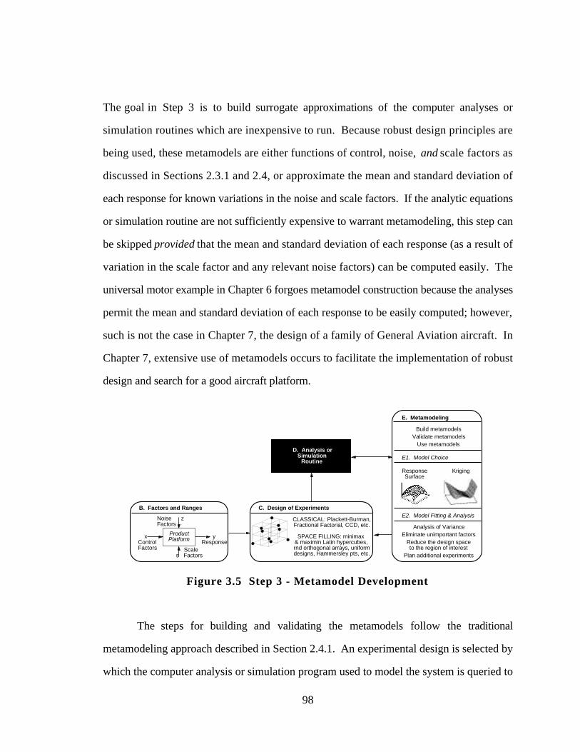
98
The goal in Step 3 is to build surrogate approximations of the computer analyses or
simulation routines which are inexpensive to run. Because robust design principles are
being used, these metamodels are either functions of control, noise, and scale factors as
discussed in Sections 2.3.1 and 2.4, or approximate the mean and standard deviation of
each response for known variations in the noise and scale factors. If the analytic equations
or simulation routine are not sufficiently expensive to warrant metamodeling, this step can
be skipped provided that the mean and standard deviation of each response (as a result of
variation in the scale factor and any relevant noise factors) can be computed easily. The
universal motor example in Chapter 6 forgoes metamodel construction because the analyses
permit the mean and standard deviation of each response to be easily computed; however,
such is not the case in Chapter 7, the design of a family of General Aviation aircraft. In
Chapter 7, extensive use of metamodels occurs to facilitate the implementation of robust
design and search for a good aircraft platform.
yResponse
Noise zFactors
xControlFactors Scale
s Factors
E. Metamodeling
B. Factors and RangesE2. Model Fitting & Analysis
Analysis of VarianceEliminate unimportant factors
Reduce the design spaceto the region of interest
Plan additional experiments
D. Analysis orSimulation
Routine
C. Design of Experiments
CLASSICAL: Plackett-Burman,Fractional Factorial, CCD, etc.
SPACE FILLING: minimax & maximin Latin hypercubes,rnd orthogonal arrays, uniformdesigns, Hammersley pts, etc.
E1. Model Choice
Build metamodelsValidate metamodels
Use metamodels
ResponseSurface
Kriging
ProductPlatform
Figure 3.5 Step 3 - Metamodel Development
The steps for building and validating the metamodels follow the traditional
metamodeling approach described in Section 2.4.1. An experimental design is selected by
which the computer analysis or simulation program used to model the system is queried to
99
obtain data. The experimental design is used to sample the design space identified by the
ranges (i.e., bounds) on the control, noise, and scale factors. The resulting sample data
then is used to build a metamodel (e.g., a kriging model, Section 2.4.2) for each response.
Model accuracy then is assessed through additional validation points or otherwise
appropriate procedures for the specific type of metamodel employed.
If identifying an appropriate region of interest for constructing the metamodels is
difficult, a sequential approximation strategy with screening experiments may be employed.
Description of such an approach can be found in, e.g., (Chen, et al., 1997; Koch, et al.,
1997; Myers and Montgomery, 1995). The difficulty, then, lies in defining an appropriate
design space. In this dissertation, the design space for the General Aviation aircraft
example problem is known, making identification of a good design space appear trivial. In
reality it is not, and there is often great difficulty finding an appropriately good design
space. Identifying and quantifying a “good” design space is not addressed in this
dissertation; it is a possibility for future work (see Section 8.3).
3 .1 .4 Step 4 - Aggregate Product Platform Specifications
Once the necessary metamodels have been built and validated, Step 4 in the PPCEM
is to aggregate the product platform specifications. This involves formulating an
appropriate compromise DSP to model the necessary constraints and goals for the product
family and product platform based on the overall design requirements, the market
segmentation developed in Step 1, and the factor classification and ranges developed in
Step 2, see Figure 3.6. It is imperative that product constraints or goals given in the overall
design requirements that are not captured within the desired platform leveraging strategy be
included in the compromise DSP.
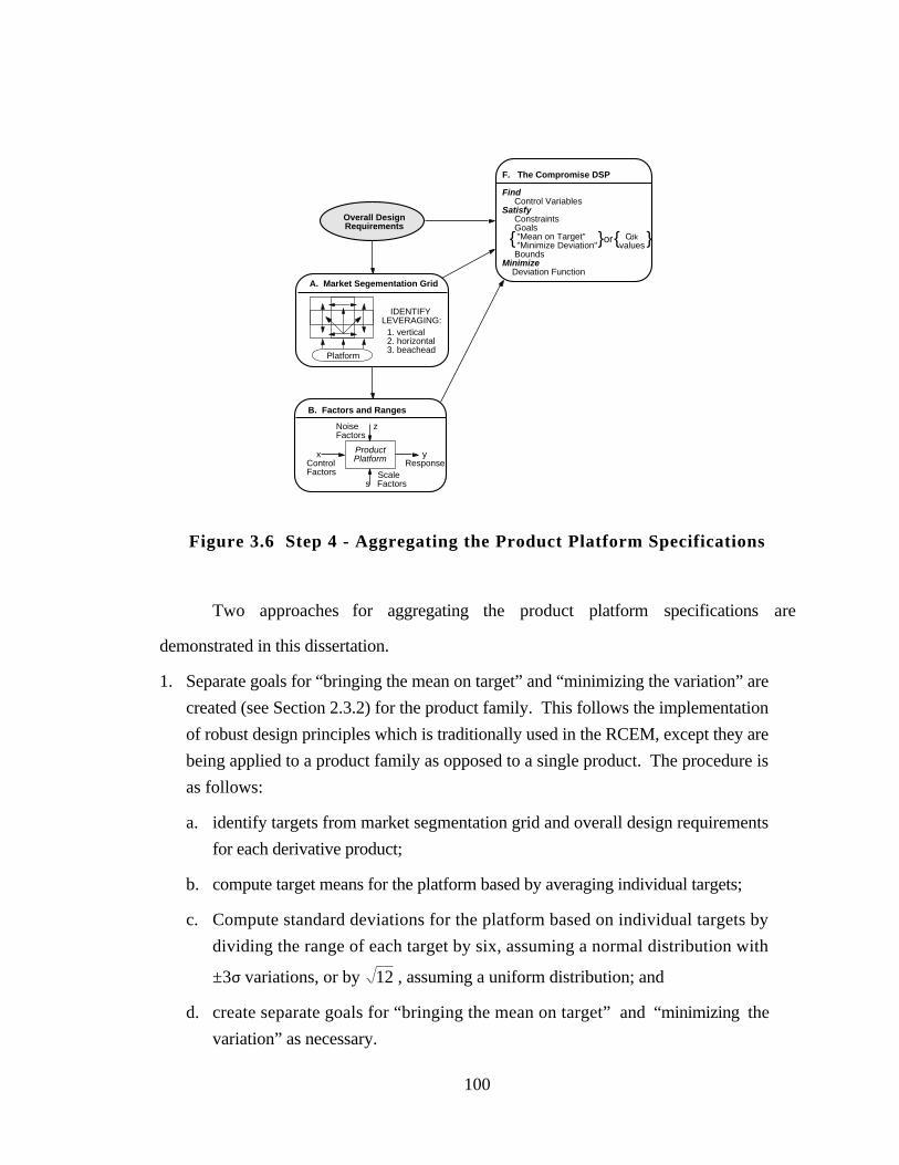
100
yResponse
Noise zFactors
xControlFactors Scale
s Factors
B. Factors and Ranges
Overall Design Requirements
ProductPlatform
F. The Compromise DSP
Find Control VariablesSatisfy Constraints Goals "Mean on Target" C "Minimize Deviation" values BoundsMinimize Deviation Function
A. Market Segementation Grid
IDENTIFYLEVERAGING:
1. vertical 2. horizontal 3. beachead
Platform
dkor{ } }{
Figure 3.6 Step 4 - Aggregating the Product Platform Specifications
Two approaches for aggregating the product platform specifications are
demonstrated in this dissertation.
1. Separate goals for “bringing the mean on target” and “minimizing the variation” are
created (see Section 2.3.2) for the product family. This follows the implementation
of robust design principles which is traditionally used in the RCEM, except they are
being applied to a product family as opposed to a single product. The procedure is
as follows:
a. identify targets from market segmentation grid and overall design requirements
for each derivative product;
b. compute target means for the platform based by averaging individual targets;
c. Compute standard deviations for the platform based on individual targets by
dividing the range of each target by six, assuming a normal distribution with
±3σ variations, or by 12 , assuming a uniform distribution; and
d. create separate goals for “bringing the mean on target” and “minimizing the
variation” as necessary.
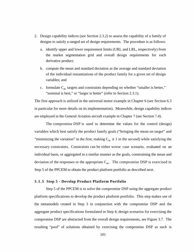
101
2. Design capability indices (see Section 2.3.2) to assess the capability of a family of
designs to satisfy a ranged set of design requirements. The procedure is as follows:
a. identify upper and lower requirement limits (URL and LRL, respectively) from
the market segmentation grid and overall design requirements for each
derivative product;
b. compute the mean and standard deviation as the average and standard deviation
of the individual instantiations of the product family for a given set of design
variables; and
c. formulate Cdk targets and constraints depending on whether “smaller is better,”
“nominal is best,” or “larger is better” (refer to Section 2.3.1).
The first approach is utilized in the universal motor example in Chapter 6 (see Section 6.3
in particular for more details on its implementation). Meanwhile, design capability indices
are employed in the General Aviation aircraft example in Chapter 7 (see Section 7.4).
The compromise DSP is used to determine the values for the control (design)
variables which best satisfy the product family goals (“bringing the mean on target” and
“minimizing the variation” in the first; making Cdk ≥ 1 in the second) while satisfying the
necessary constraints. Constraints can be either worse case scenario, evaluated on an
individual basis, or aggregated in a similar manner as the goals, constraining the mean and
deviation of the responses or the appropriate Cdk . The compromise DSP is exercised in
Step 5 of the PPCEM to obtain the product platform portfolio as described next.
3 .1 .5 Step 5 - Develop Product Platform Portfolio
Step 5 of the PPCEM is to solve the compromise DSP using the aggregate product
platform specifications to develop the product platform portfolio. This step makes use of
the metamodels created in Step 3 in conjunction with the compromise DSP and the
aggregate product specifications formulated in Step 4; design scenarios for exercising the
compromise DSP are abstracted from the overall design requirements, see Figure 3.7. The
resulting “pool” of solutions obtained by exercising the compromise DSP as such is
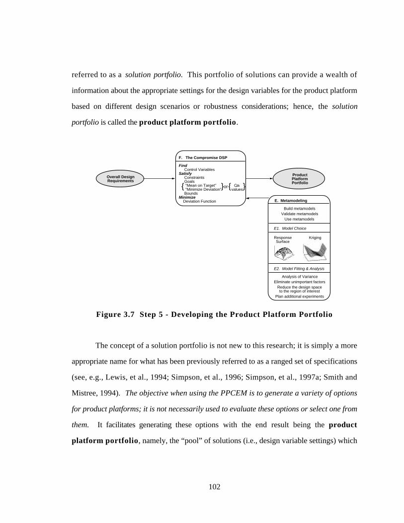
102
referred to as a solution portfolio. This portfolio of solutions can provide a wealth of
information about the appropriate settings for the design variables for the product platform
based on different design scenarios or robustness considerations; hence, the solution
portfolio is called the product platform portfolio.
ProductPlatformPortfolio
E. Metamodeling
Overall Design Requirements
E2. Model Fitting & Analysis
Analysis of VarianceEliminate unimportant factors
Reduce the design spaceto the region of interest
Plan additional experiments
E1. Model Choice
Build metamodelsValidate metamodels
Use metamodels
ResponseSurface
Kriging
F. The Compromise DSP
Find Control VariablesSatisfy Constraints Goals "Mean on Target" C "Minimize Deviation" values BoundsMinimize Deviation Function
dkor{ } }{
Figure 3.7 Step 5 - Developing the Product Platform Portfolio
The concept of a solution portfolio is not new to this research; it is simply a more
appropriate name for what has been previously referred to as a ranged set of specifications
(see, e.g., Lewis, et al., 1994; Simpson, et al., 1996; Simpson, et al., 1997a; Smith and
Mistree, 1994). The objective when using the PPCEM is to generate a variety of options
for product platforms; it is not necessarily used to evaluate these options or select one from
them. It facilitates generating these options with the end result being the product
platform portfolio, namely, the “pool” of solutions (i.e., design variable settings) which

103
should be maintained in order for the product platform to have sufficient flexibility to meet
the desired design scenarios in the event that one scenario is preferred to the next.
In addition to developing the product platform portfolio for the product family,
product variety tradeoff studies also can be performed by making use of two measures—
the Non-Commonality Index (NCI) and the Performance Deviation Index (PDI)—which
are described as follows:
Non-commonality Index (NCI): NCI is used to assess the amount of variation
between parameter settings of each product within a product family; the smaller the
variation, the smaller NCI, and the more common the products within the product
family. Computing NCI is perhaps best illustrated through example; consider the 3
products shown in Figure 3.8. Assume that each product is described by three
design variables: x1, x2, and x3 (if these three hypothetical products were electric
motors, then x1, x2, and x3 might be the outer radius of the motor, the length of the
motor, and the number of windings in the motor). First, the dissimilarity of each
design variable settings for each product within the family is computed as follows:
1. Compute the mean of each of the xj within the product family and the absolute
value of the difference between µj and xj for each of the i products.
2. Normalize each difference by the range of that particular design variable: [upper
bound (ubj) - lower bound (lbj)]; this measures the relative variation in the
values of the design variables to the total range for that design variable.
3. Compute the average of the resulting normalized differences; this value is
denoted DIi in the figure and is the dissimilarity of the settings of xi for the
group of products.
The scale factor around which the product family is derived is not included in this
computation. NCI is taken as a weighted sum of the individual DIi, where the
weights reflect the relative difficulty or cost associated with allowing each parameter
to vary. For an electric motor for instance, it may be easier or cheaper to allow the
number of windings (x3) to vary between different motor models but not so to
allow the outer radius to vary (x1). In this case, w1 would be much larger than w3
to reflect this within the product family.
104
2 3
µ1
10 20
µ2
0 100
µ3
Pro
duct
1
Pro
duct
2
Pro
duct
3
x1: 2.5 2.5 2.8
x2: 12.1 10.0 10.9
x3: 13.0 18.0 35.0
DI 3 =1
3
22 −13 + 22−18 + 22− 35
(100 − 0)
DI3 = 0.0867
DI j =1n
µ j − x i,j
ub j − lb j( )i=1
n
∑
j = 1, ..., # design variables
i = 1, ..., # products in family
DI 2 =1
3
11−12.1 + 11−10 + 11−10.9
(20−10)
DI 2 = 0.0733
Product Descriptions
Dissimilarity Index
Dissimilarity of x1
Dissimilarity of x2
Dissimilarity of x3
DI 1 =1
3
2.6 − 2.5 + 2.6 − 2.5 + 2.6 − 2.8
(3 −2)
DI1 = 0.133
DisIndx = w jDI j = 0.55(0.133)+j=1
#d.v.
∑ 0.3(0.0733) + 0.15(0.0867) = 0.108NCI =Non-commonality Index:
Figure 3.8 Estimating the Dissimilarity Index for a Product Family
Performance Deviation Index: Assuming that a market niche is defined by a set
of goal targets and constraints and that the necessary constraints are met for each
individual derivative product, then the deviation variables in the compromise DSP
are a direct measure of how well each derivative product meets its targets. The
Performance Deviation Index (PDI) for a product family thus is taken as a linear
combination (possibly weighted) of the deviation variables for each derivative
product within the product family as given by Equation 3.1:
PDI = wiZ ii=1
n
∑ [3.1]
where i = {1, ..., # products in family}, and Zi is the corresponding deviation
function for each derivative product within the product family. Weightings may be
used to bias the measure for certain products within the family.
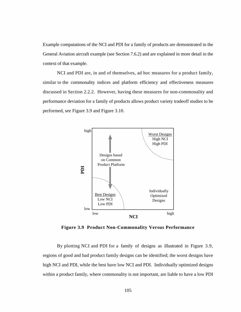
105
Example computations of the NCI and PDI for a family of products are demonstrated in the
General Aviation aircraft example (see Section 7.6.2) and are explained in more detail in the
context of that example.
NCI and PDI are, in and of themselves, ad hoc measures for a product family,
similar to the commonality indices and platform efficiency and effectiveness measures
discussed in Section 2.2.2. However, having these measures for non-commonality and
performance deviation for a family of products allows product variety tradeoff studies to be
performed, see Figure 3.9 and Figure 3.10.
NCI
PD
I
low
high
low high
Best DesignsLow NCILow PDI
Worst DesignsHigh NCIHigh PDI
IndividuallyOptimizedDesigns
Designs basedon Common
Product Platform
Figure 3.9 Product Non-Commonality Versus Performance
By plotting NCI and PDI for a family of designs as illustrated in Figure 3.9,
regions of good and bad product family designs can be identified; the worst designs have
high NCI and PDI, while the best have low NCI and PDI. Individually optimized designs
within a product family, where commonality is not important, are liable to have a low PDI
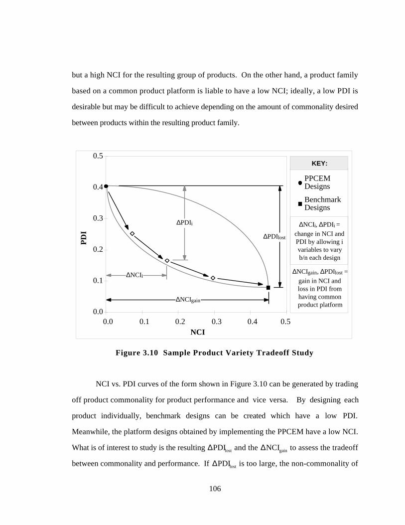
106
but a high NCI for the resulting group of products. On the other hand, a product family
based on a common product platform is liable to have a low NCI; ideally, a low PDI is
desirable but may be difficult to achieve depending on the amount of commonality desired
between products within the resulting product family.
0.0
0.1
0.2
0.3
0.4
0.5
0.0 0.1 0.2 0.3 0.4 0.5NCI
PD
I
∆NCIgain, ∆PDIlost =
gain in NCI andloss in PDI fromhaving commonproduct platform
PPCEMDesigns
BenchmarkDesigns
KEY:
∆PDIlost
∆NCIgain
∆PDIi
∆NCIi
∆NCIi, ∆PDIi =
change in NCI and PDI by allowing i variables to vary b/n each design
Figure 3.10 Sample Product Variety Tradeoff Study
NCI vs. PDI curves of the form shown in Figure 3.10 can be generated by trading
off product commonality for product performance and vice versa. By designing each
product individually, benchmark designs can be created which have a low PDI.
Meanwhile, the platform designs obtained by implementing the PPCEM have a low NCI.
What is of interest to study is the resulting ∆PDIlost and the ∆NCIgain to assess the tradeoff
between commonality and performance. If ∆PDIlost is too large, the non-commonality of
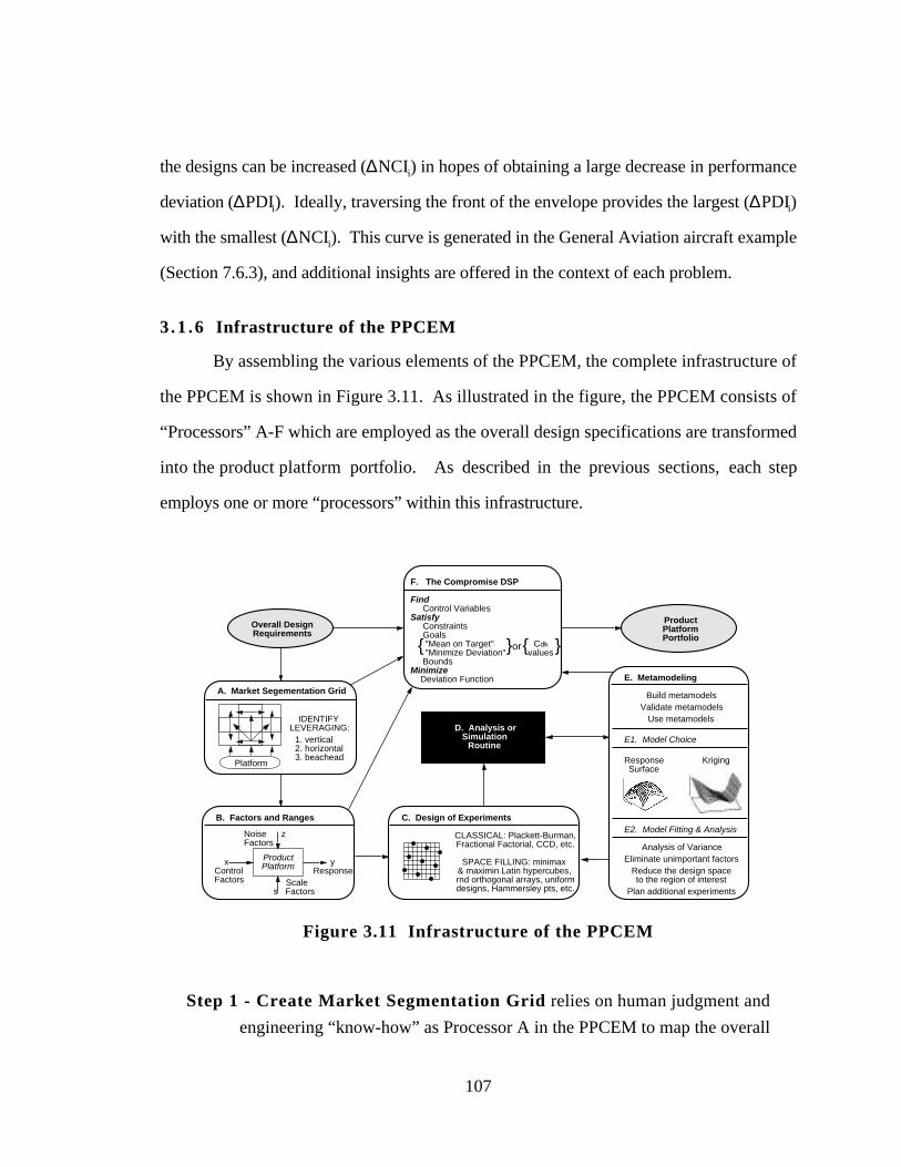
107
the designs can be increased (∆NCIi) in hopes of obtaining a large decrease in performance
deviation (∆PDIi). Ideally, traversing the front of the envelope provides the largest (∆PDIi)
with the smallest (∆NCIi). This curve is generated in the General Aviation aircraft example
(Section 7.6.3), and additional insights are offered in the context of each problem.
3 .1 .6 Infrastructure of the PPCEM
By assembling the various elements of the PPCEM, the complete infrastructure of
the PPCEM is shown in Figure 3.11. As illustrated in the figure, the PPCEM consists of
“Processors” A-F which are employed as the overall design specifications are transformed
into the product platform portfolio. As described in the previous sections, each step
employs one or more “processors” within this infrastructure.
yResponse
Noise zFactors
xControlFactors Scale
s Factors
ProductPlatformPortfolio
E. Metamodeling
B. Factors and Ranges
Overall Design Requirements
E2. Model Fitting & Analysis
Analysis of VarianceEliminate unimportant factors
Reduce the design spaceto the region of interest
Plan additional experiments
D. Analysis orSimulation
Routine
C. Design of Experiments
CLASSICAL: Plackett-Burman,Fractional Factorial, CCD, etc.
SPACE FILLING: minimax & maximin Latin hypercubes,rnd orthogonal arrays, uniformdesigns, Hammersley pts, etc.
E1. Model Choice
Build metamodelsValidate metamodels
Use metamodels
ResponseSurface
Kriging
ProductPlatform
F. The Compromise DSP
Find Control VariablesSatisfy Constraints Goals "Mean on Target" C "Minimize Deviation" values BoundsMinimize Deviation Function
A. Market Segementation Grid
IDENTIFYLEVERAGING:
1. vertical 2. horizontal 3. beachead
Platform
dkor{ } }{
Figure 3.11 Infrastructure of the PPCEM
Step 1 - Create Market Segmentation Grid relies on human judgment and
engineering “know-how” as Processor A in the PPCEM to map the overall
108
design requirements into an appropriate market segmentation grid and
identify leveraging opportunities.
Step 2 - Classify Factors and Ranges relies on the human judgment and
Processor B in the PPCEM to map the overall design requirements and
market segmentation grid into appropriate control, noise, and scale factors
and identify corresponding ranges for each. The responses being
investigated also need to be identified in this step of the process.
Step 3 - Build and Validate Metamodels relies on human judgment and
Processors C, D, and E for construction and validation of the necessary
metamodels.
Step 4 - Aggregate Product Platform Specifications relies on human
judgment to formulate a compromise DSP, Processor F, using information
from Processors A and B and the overall design requirements.
Step 5 - Develop the Product Platform Portfolio involves exercising
Processor F in combination with the metamodels in Processor E to obtain
the product platform portfolio which best satisfies the given overall design
requirements.
Referring back to Figure 1.5, the structure of the PPCEM is very similar to the
RCEM; this is not a coincidence. In essence, the PPCEM is derived from the RCEM
through a series of modifications based on the research questions and hypotheses presented
in Section 1.3.1. The research hypotheses are revisited next.
3.2 RESEARCH HYPOTHESES AND POSITS FOR THE PPCEM
As stated in Section 1.3, there are three main hypotheses in this dissertation:
Hypothesis 1: The Product Platform Concept Exploration Method provides a
method for developing a scalable product platform for a product family.
109
Hypothesis 2: Kriging is a viable alternative for building metamodels of
deterministic computer analyses.
Hypothesis 3: Space filling experimental designs are better suited for building
metamodels of deterministic computer experiments than classical experimental
designs.
As discussed in Section 1.3.1, Hypotheses 2 and 3 help to support Hypothesis 1 by
increasing the efficiency of the PPCEM but have ramifications beyond the PPCEM itself.
To facilitate verification of Hypothesis 1, three sub-hypotheses have been formulated; these
sub-hypotheses are as follows:
Sub-Hypothesis 1.1: The market segmentation grid can be utilized to help
identify scale factors for a product platform.
Sub-Hypothesis 1.2: Robust design principles can be used to facilitate the
design of a common scalable product platform by minimizing the sensitivity of a
product platform to variations in scale factors.
Sub-Hypothesis 1.3: Individual targets for product variants can be aggregated
into an appropriate mean and variance and used in conjunction with robust
design principles to effect a common product platform for a product family .
It is upon these hypotheses that the PPCEM and the work in this dissertation are
grounded. The relationship between these hypotheses and the modifications to RCEM
which form the PPCEM are presented in the next section. This is followed in Section
3.2.2 with supporting posits for the research hypotheses.
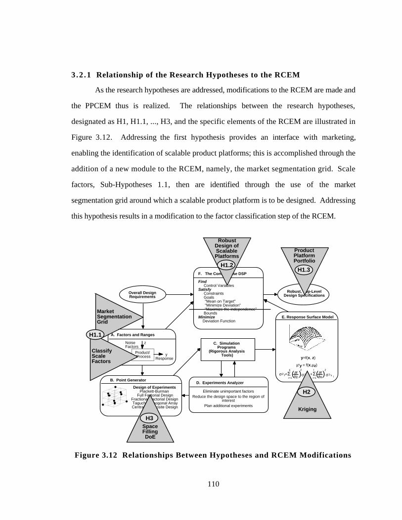
110
3 .2 .1 Relationship of the Research Hypotheses to the RCEM
As the research hypotheses are addressed, modifications to the RCEM are made and
the PPCEM thus is realized. The relationships between the research hypotheses,
designated as H1, H1.1, ..., H3, and the specific elements of the RCEM are illustrated in
Figure 3.12. Addressing the first hypothesis provides an interface with marketing,
enabling the identification of scalable product platforms; this is accomplished through the
addition of a new module to the RCEM, namely, the market segmentation grid. Scale
factors, Sub-Hypotheses 1.1, then are identified through the use of the market
segmentation grid around which a scalable product platform is to be designed. Addressing
this hypothesis results in a modification to the factor classification step of the RCEM.
E. Response Surface Model
y=f(x, z)
µˆy = f(x,µz)
σ2ˆy=Σi=1
k∂f∂zi( )
2
σ2ˆz i i=1
l∂f∂xi( )
2
σ2ˆx i+Σ
Robust, Top-LevelDesign Specifications
Overall Design Requirements
A. Factors and Ranges
Product/ Process
Noise zFactors
yResponse
xControlFactors
B. Point Generator
Design of ExperimentsPlackett-Burman
Full Factorial DesignFractional Factorial DesignTaguchi Orthogonal ArrayCentral Composite Design
etc.
C. Simulation Programs
(Rigorous Analysis Tools)
F. The Compromise DSP
Find Control VariablesSatisfy Constraints Goals "Mean on Target" "Minimize Deviation" “Maximize the independence” BoundsMinimize Deviation Function
D. Experiments Analyzer
Eliminate unimportant factorsReduce the design space to the region of
interestPlan additional experiments
ProductPlatformPortfolio
SpaceFillingDoE
MarketSegmentationGrid
ClassifyScaleFactors
H1.1
H3
Kriging
H2
H1.3
RobustDesign ofScalablePlatforms
H1.2
Figure 3.12 Relationships Between Hypotheses and RCEM Modifications
111
Sub-Hypothesis 1.2 relates to designing the actual product platform; robust design
principles are abstracted for use in product family design by aggregating product family
targets and constraints into appropriate means and variances. The resulting formulation
allows robust design principles, already embodied in the RCEM in the form of separate
goals for “bringing the mean on target” and “minimizing the variation,” to be utilized when
solving the compromise DSP. Notice that the goal for “minimize the independence” is not
included in the compromise DSP formulation because the intent is to rely solely on robust
design principles to designing a suitable product platform which can be scaled into a
product family. As the research hypotheses are addressed and the RCEM is
correspondingly modified, the PPCEM is realized; compare Figure 3.12 to Figure 3.11.
Hypotheses 2 and 3 relate specifically to the metamodeling capabilities of the
RCEM with Hypothesis 2 affecting Processor E and Hypothesis 3 affecting Processor B as
shown in Figure 3.12. The intent is not to replace the current response surface and design
of experiments capabilities of the RCEM; rather, it is to augment the current capabilities
with kriging and novel space filling experimental designs, enabling better approximations
of deterministic computer experiments. The specific posits which support these claims and
the research hypotheses are detailed in the next section.
3 .2 .2 Supporting Posits for the Research Hypotheses
There are several posits which support the research hypotheses which have been
revealed during the literature review in Chapter 2 and in the discussion in Section 1.1. Six
posits support Hypotheses 1 and Sub-Hypotheses 1.1-1.3.; they are the following:
Posit 1.1: The RCEM provides an efficient and effective means for developing
robust top-level design specifications for complex systems design.
112
Posit 1.2: Metamodeling techniques, specifically, design of experiments and the
response surface methodology, can be used to facilitate concept exploration and
optimization, thus increasing a designer’s efficiency.
Posit 1.3: Robust design principles can be used to minimize the sensitivity of a
design to variations in uncontrollable (i.e., noise) factors and/or variations in
design parameters (i.e., control factors).
Posit 1.4: Robust design principles can be used effectively in the early stages of the
design process by modeling the response itself with separate goals for “bringing
the mean on target” and “minimizing the variation.”
Posit 1.5: The compromise DSP is capable of effecting robust design solutions
through separate goals for “bringing the mean on target” and “minimizing
variation” of noise factors and/or variations in the design variables.
Posit 1.6: The market segmentation grid can be used to identify opportunities for
platform leveraging in product family design.
These posits are founded on and substantiated by the following references.
• Posit 1.1 is substantiated in (Chen, 1995) by explicitly testing and verifying the
efficiency and effectiveness of the RCEM for developing robust top-level design
specifications for complex systems design.
• Posit 1.2 is substantiated through the numerous applications of design of
experiments and response surface models that have been used to illustrate the
usefulness of metamodeling techniques in design, facilitating concept exploration
and optimization and increasing a designer’s efficiency; over twenty-five such
applications are reviewed in (Simpson, et al., 1997b). Furthermore, Chen (1995)
explicitly tests and verifies this posit as part of the development of the RCEM.
• Posit 1.3, Posit 1.4, and Posit 1.5 are substantiated by the work in (Chen, et al.,
1996b); Chen and her coauthors describe a general robust design procedure which
can minimize the sensitivity of a design to variations in noise factors and/or design
113
parameters (Posit 1.3) by having separate goals for “bringing the mean on target”
and “minimizing the variation” (Posit 1.4) of each response in the compromise DSP
(Posit 1.5). These posits are further substantiated in (Chen, 1995) as part of the
development of the RCEM.
• Posit 1.6 is substantiated by the discussion in Section 2.2.1, i.e., the market
segmentation grid can be used as an attention directing tool to identify leveraging
opportunities in product platform design (cf., Meyer, 1997; Meyer and Lehnerd,
1997); identifying these leveraging opportunities provided the initial impetus for
developing the market segmentation grid.
These six posits help to support Hypothesis 1 and Sub-Hypotheses 1.1-1.3. The strategy
for testing and verifying these hypotheses is outlined in Section 3.3. Before the
verification strategy is outlined, however, posits for Hypotheses 2 and 3 are stated.
The following two posits have been identified in support of Hypothesis 2.
Posit 2.1: Building an interpolative kriging model is not predicated on the
assumption of underlying random error in the data.
Posit 2.2: Kriging provides very flexible modeling capabilities based on the wide
variety of spatial correlation functions which can be selected to model the data.
• Posit 2.1 is more fact than assumption; it is substantiated by, e.g., Sacks, et al.
(1989); Koehler and Owen (1996); and Cressie (1993).
• Posit 2.2 is substantiated by many researchers, most notably Sacks, et al. (1989);
Welch, et al. (1992); Cressie (1993); and Barton (1992; 1994).
Posits 2.1 and 2.2 both help to verify Hypothesis 2; the strategy for testing Hypothesis 2 is
outlined in Section 3.3.
Finally, the following two posits support Hypothesis 3:
114
Posit 3.1: The experimental design conditions of replication, blockability,
rotatability have no significant meaning when sampling deterministic computer
experiments.
• Posit 3.1 is taken from Sacks, et al. (1989) who state that the “classical notions of
experimental blocking, replication, and randomization are irrelevant” for
deterministic computer experiments which contain no random error. Moreover, any
experimental design text (see, e.g., Montgomery, 1991) can verify that replication,
blockability, and rotatability are developed explicitly to handle and account for
random (measurement) error in a physical experiment for which classical
experimental designs have been developed.
Since kriging (using an underlying constant model) is being advocated in this
dissertation for metamodeling deterministic computer experiments, an additional posit in
support of Hypothesis 3 is the following.
Posit 3.2: Since kriging (with an underlying constant model) models rely on the
spatial correlation between data, confounding and aliasing of main effects and
two-factor interactions have no significant meaning when predicting a response.
• Posit 3.2 is substantiated by Sacks, et al. (1989); Currin, et al. (1991); Welch, et
al. (1990); and Barton (1992; 1994). In physical experimentation, great care is
taken to ensure that aliasing and confounding of main effects and two-factor
interactions do not occur to ensure accurate estimation of coefficients of the
polynomial response surface model (see, e.g., Montgomery, 1991).
The experimental procedure for testing Hypothesis 3 is introduced in the next section along
with the specific strategy for verification and testing of all of the other hypotheses.

115
3.3 STRATEGY FOR VERIFICATION AND TESTING OF THERESEARCH HYPOTHESES
The question of whether testing the proposed hypotheses really answers the
research questions is a difficult one, and it raises the issues of verification and validation as
discussed by Peplisnki (1997). According to the Concise Oxford English Dictionary
(1982), to validate is to make valid, to ratify or confirm. The root, valid, is then defined
as:
• (of reason, objection, argument, etc.) sound, defensible, well-grounded;
• (law) sound and sufficient, executed with proper formalities (valid contract);
• legally acceptable (valid passport).
With respect to engineering design research, the intent of the validation process is to show
the research and its products to be sound, well grounded on principles of evidence, able to
withstand criticism or objection, powerful, convincing and conclusive, and provable.
In the Merriam-Webster hypertext dictionary under a discussion of the synonyms
for “confirm”, “verify” is used in the context of establishing the correspondence of actual
facts or details with those proposed or guessed at, while “validate” is used in the context of
establishing validity by authoritative affirmation or by factual proof. The boundary
between verification and validation is thus shifting and often open to interpretation; in many
cases the two words are used interchangeably.
In this research, definitions for “verification” and “validation” are applied that,
while not inconsistent with the general uses above, are more specific and tailored for efforts
in engineering design research. In practice, the verification and validation of design
methods is much more than a debugging process. Three primary phases can be identified:
firstly, problem justification; secondly, completeness and consistency checks of the
methodology, and thirdly, validation of performance. (This classification is based on a
discussion of the validation of expert systems by Ignizio (1990).) Verification then

116
refers to the second phase of the process and is focused primarily on internal consistency
and completeness, while validation as the third phase of the process is focused on
consistency with external evidence, ideally through testing the design method on actual case
studies. This validation of performance is perhaps the area most open to interpretation by
peers and experts in the field alike.
If what is to be validated is a closed form mathematical expression or algorithm, it
can be proven, or validated, in a traditional and formal mathematical sense. For example,
the case of showing a solution vector, x , belongs to the set of feasible solutions for a given
mathematical model is a closed problem. Alternatively, if the problem is open, if the
subject is dealing with some “heuristic,” non-precise scheme, the issue of validation
becomes one of “correctness beyond reasonable doubt.” The validation of design methods
falls into this category. In this case it is achieved ultimately by results and usefulness and
through a convincing demonstration to (and an acceptance and ratification by) one’s peers
in the field. An analogy with mathematics and the concept of “necessary” and “sufficient”
conditions can be drawn with respect to the validation of heuristics. Heuristics are aimed
toward satisfying the necessary conditions only; it is not possible to develop an absolute
proof for an open problem by definition.
As anticipated, the operations research literature provides some useful insight into
the validation of heuristics, in the context of heuristic programming. In discussing the
nature of problem solving by heuristic programming Lin (1975) makes the following
remarks:
We therefore define a valid heuristic algorithm (to solve a given problem) as anyprocedure which will produce a feasible solution acceptable to the designengineer, within limits of computing time, and consider the problem solved ifwe can construct a valid heuristic procedure to solve it. We see that in thedomain where a heuristic algorithm operates, there are elements of technique,experimentation, judgment and persuasion, as well as compromise.
The issue of justification is addressed by Ignizio, et al. (1972):
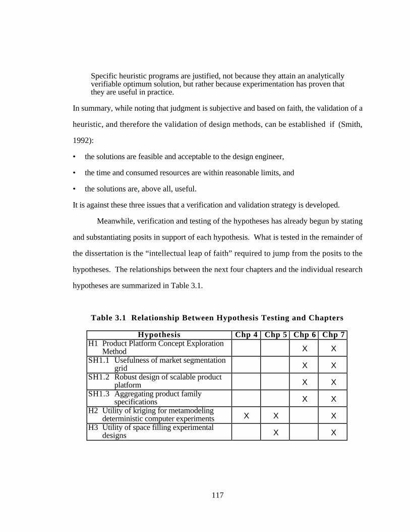
117
Specific heuristic programs are justified, not because they attain an analyticallyverifiable optimum solution, but rather because experimentation has proven thatthey are useful in practice.
In summary, while noting that judgment is subjective and based on faith, the validation of a
heuristic, and therefore the validation of design methods, can be established if (Smith,
1992):
• the solutions are feasible and acceptable to the design engineer,
• the time and consumed resources are within reasonable limits, and
• the solutions are, above all, useful.
It is against these three issues that a verification and validation strategy is developed.
Meanwhile, verification and testing of the hypotheses has already begun by stating
and substantiating posits in support of each hypothesis. What is tested in the remainder of
the dissertation is the “intellectual leap of faith” required to jump from the posits to the
hypotheses. The relationships between the next four chapters and the individual research
hypotheses are summarized in Table 3.1.
Table 3.1 Relationship Between Hypothesis Testing and Chapters
Hypothesis Chp 4 Chp 5 Chp 6 Chp 7H1 Product Platform Concept Exploration
Method X XSH1.1 Usefulness of market segmentation
grid X XSH1.2 Robust design of scalable product
platform X XSH1.3 Aggregating product family
specifications X XH2 Utility of kriging for metamodeling
deterministic computer experiments X X XH3 Utility of space filling experimental
designs X X
118
The relationships listed in Table 3.1 are elaborated further in the next two sections.
The strategy for testing Hypothesis 1 and the related sub-hypotheses is outlined in Section
3.3.1. The strategy for testing Hypotheses 2 and 3 is outlined in Section 3.3.2.
3 .3 .1 Testing Hypothesis 1 and Sub-Hypotheses 1.1-1.3
The PPCEM is hypothesized to provide a method for designing a scalable product
platform for a product family. To verify this, two example problems are utilized to
demonstrate the effectiveness of the PPCEM: the design of a family of universal electric
motors (Chapter 6) and the design of a family of General Aviation aircraft (Chapter 7).
These two examples have been chosen to demonstrate different capabilities of the PPCEM.
• Design of a family of universal electric motors is used to demonstrate the following:
- vertical scaling of a product platform (see Section 6.2),
- a parametric scale factor: stack length (see Section 6.2), and
- product family aggregated around mean and standard deviation of stack length
and separate goals for “bringing the mean on target” and “minimize the
variation” are employed to design the product platform (see Section 6.3).
Note that metamodels are not employed in this first example because mean and standard
deviation of the responses can be estimated directly from the relevant analysis equations
(see Section 6.3).
• Design of a family of General Aviation aircraft is used demonstrate the following:
- horizontal scaling of a product platform (see Section 7.1.3),
- a configurational scale factor: number of passengers (see Section 7.2),
- metamodels for mean and standard deviation of the GAA family to facilitate
implementation of robust design and development of the aircraft platform (see
Section 7.3), and
- design capability indices to assess quickly the capability of the family of aircraft
to satisfy the range of requirements (see Section 7.4).
119
The first example parallels Black & Decker’s vertical scaling strategy for its universal
motors (Lehnerd, 1987) discussed in Section 1.1.1 and is used to provide “proof of
concept” that the PPCEM works. The second example is based on a previous application
of the RCEM to develop a “common and good” set of top-level design specifications for a
family of General Aviation aircraft (see, e.g., Simpson, 1995; Simpson, et al., 1996). The
General Aviation aircraft problem is employed in this work to demonstrate further the
effectiveness of the PPCEM while exploring the problem itself in greater depth.
In each example, the product platform obtained using the PPCEM is compared to
(a) the initial baseline design to show improvement over the starting design, and (b)
individually designed, benchmark products which are aggregated into a product family to
provide a reference to compare against the PPCEM product family (i.e., design the family
of products with the PPCEM and without the PPCEM and discuss the differences in
product performance, computational expense, and usefulness). Product variety tradeoff
studies are also performed for the family of General Aviation aircraft, examining the
tradeoff between commonality of the aircraft and their corresponding performance for the
PPCEM family and the individually designed benchmark group of aircraft.
Testing of the sub-hypotheses related to Hypotheses 1 entail the following:
Testing Sub-Hypothesis 1.1 - The procedure for using the market segmentation
grid to identify scale factors for a product platform is shown in Figure 3.4 and
described in Section 3.1.2. Further verification of this sub-hypothesis requires
demonstrating that this procedure can be used to identify scale factors for a product
platform. In the universal motor example in Chapter 6, the market segmentation
grid is used to identify a vertical leveraging strategy and parametric scaling factor
(stack length); in the General Aviation aircraft example, a horizontal leveraging
strategy and configurational scale factor (number of passengers) are used.
Testing Sub-Hypothesis 1.2 - If appropriate scale factors can be identified for a
product platform (i.e., if Sub-Hypothesis 1.1 is true), then the principles of robust
design can be employed to develop a product platform which has minimum
120
sensitivity to variations in the scale factor and is thus robust for the product family.
Verification of this sub-hypothesis requires implementation of the approach, and the
two examples provide such a demonstration.
Testing Sub-Hypothesis 1.3 - The procedure for aggregating the individual targets
of the product variants is outlined in Section 3.1.4. As with Sub-Hypothesis 1.1,
further verification of this sub-hypothesis requires demonstrating that this
procedure can be used to model and design a family of products; the approaches
outlined in Section 3.1.4 are used in the two examples to illustrate both methods for
aggregating product family specifications.
Verification of these sub-hypotheses also helps to support Hypothesis 1.
3 .3 .2 Testing Hypotheses 2 and 3
The testing of Hypotheses 2 and 3 occurs predominantly in Chapter 5; however, an
initial feasibility study of the utility of kriging is presented in Chapter 4 to familiarize the
reader with kriging. In Chapter 4, a simple yet realistic engineering example—the design
of an aerospike nozzle—is used to compare the predictive capability of a kriging model
against that of second-order response surfaces. The specific aspect of Hypothesis 2 being
tested in Section 4.2 is whether or not kriging, using an underlying constant global model
in combination with a Gaussian correlation function (one of the five being investigated in
this dissertation, see section 2.4.2) is as accurate of a predictor of the response values as a
full second-order response surface.
Chapter 5 continues from where Chapter 4 leaves off. To test the utility of kriging
and space filling designs (and thus Hypotheses 2 and 3) a testbed of six engineering test
problems is created to:
• test the effect of different correlation functions on the accuracy of the kriging model
for a wide variety of engineering analysis equations (linear, quadratic, cubic,
reciprocal, exponential, etc.);
• correlate the types of functions (analysis equations) which kriging models can and
cannot approximate accurately; and
121
• test the effect of eleven different experimental designs on the accuracy of the
resulting kriging model.
Of the eleven experimental designs mentioned in the last bullet, two are classical designs—
central composite and Box-Behnken—and the remaining nine are space filling (see Section
5.1.3 and Appendices B and C for a description of each). In this manner, Hypothesis 3 is
explicitly tested by comparing the accuracy of the kriging model built from a space filling
experimental design against that of a classical experimental design. The first two bullets
relate to testing Hypothesis 2, and the particulars of that portion of the study are described
in Section 5.2. A detailed overview of the whole study is offered in Section 5.1.
3.4 A LOOK BACK AND A LOOK AHEAD
The elements of the previous chapters are synthesized in this chapter to meet the
principal objective in this dissertation, namely, to develop the Product Platform Concept
Exploration Method (PPCEM) for designing common scalable product platforms for a
product family, see Figure 3.13. There are five steps to the PPCEM which prescribe how
to formulate the problem and describe how to solve it. As such, the PPCEM provides a
Method which facilitates the synthesis and Exploration of a common Product Platform
Concept which can be scaled into an appropriate family of products.
Testing and verification of the PPCEM is outlined in the previous section and takes
place predominantly in Chapters 6 and 7 of the dissertation. In the meantime, testing of
Hypothesis 2 (which has implications for Step 3 of the PPCEM) commences in the next
chapter wherein an initial feasibility study of the utility of kriging is given. At the end of
Chapter 4, several questions are posed which preface the kriging/DOE study in Chapter 5.
The implications of the results of the study on metamodeling within the PPCEM (Step 3)
are discussed at the end of Chapter 5.
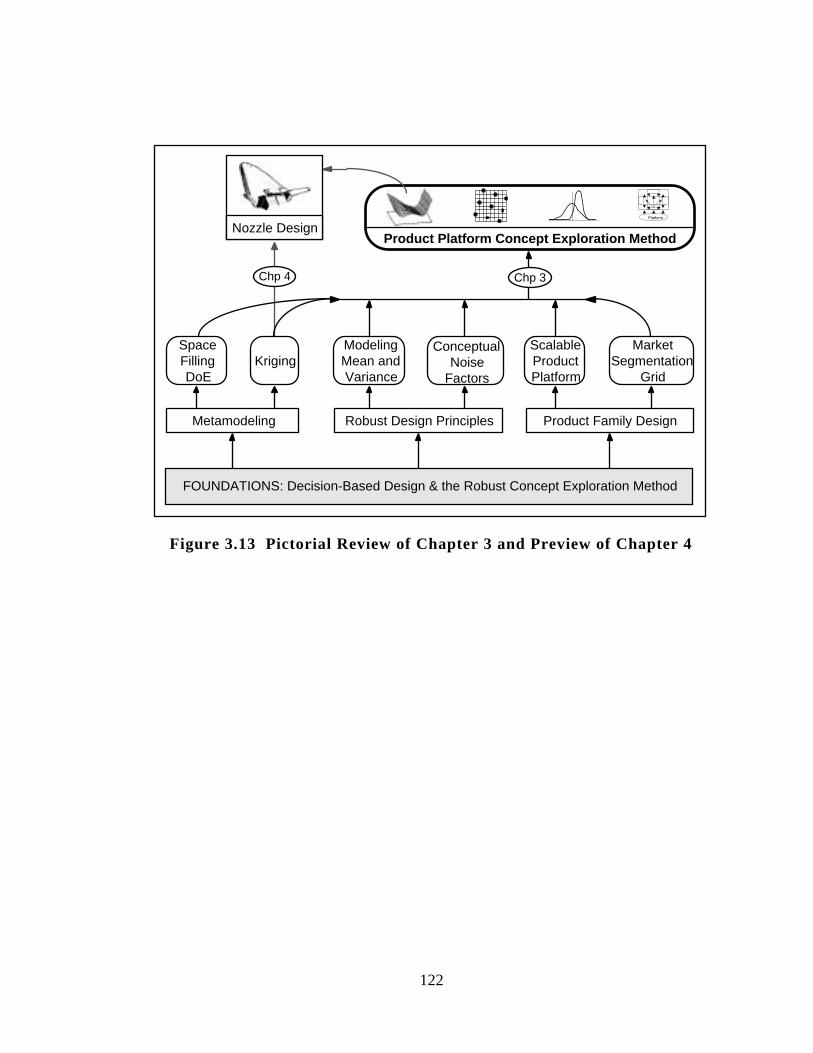
122
Metamodeling
ModelingMean andVariance
Robust Design Principles
ConceptualNoise
Factors
ScalableProductPlatform
MarketSegmentation
Grid
Product Family Design
KrigingSpaceFillingDoE
Chp 4 Chp 3
FOUNDATIONS: Decision-Based Design & the Robust Concept Exploration Method
Platform
Product Platform Concept Exploration MethodNozzle Design
Figure 3.13 Pictorial Review of Chapter 3 and Preview of Chapter 4
123
4. CHAPTER 4
INITIAL KRIGING FEASIBILITY STUDY:DESIGN OF AN AEROSPIKE NOZZLE
Nozzle Design
In this chapter, the process of testing Hypothesis 2 and establishing kriging as a
viable alternative for approximating deterministic computer experiments commences. In
particular, the accuracy of simple kriging models is compared to that of second-order
response surface models through two examples. The first is a simple one-dimensional
example in Section 4.1 which is used to familiarize the reader with (a) the process of
creating a kriging model and (b) some of the differences between a kriging model and a
second-order response surface. The second example is a simple, yet realistic, engineering
problem—the design of an aerospike nozzle—which is given in Section 4.2. In the
aerospike nozzle example, a comparison of second-order response surface models and
kriging models is conducted by means of error analysis (Section 4.2.2), visualization
(Section 4.2.3), and optimization (Section 4.2.4) These examples establish that a simple
kriging model can compete with a second-order response surface, thereby setting the stage
for an extensive investigation into the utility of kriging and space filling experimental
designs in Chapter 5 to test Hypotheses 2 and Hypothesis 3.
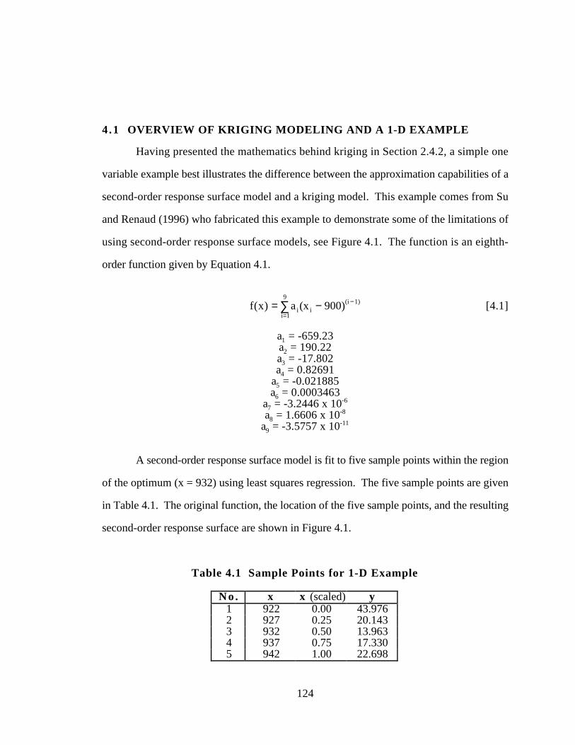
124
4.1 OVERVIEW OF KRIGING MODELING AND A 1-D EXAMPLE
Having presented the mathematics behind kriging in Section 2.4.2, a simple one
variable example best illustrates the difference between the approximation capabilities of a
second-order response surface model and a kriging model. This example comes from Su
and Renaud (1996) who fabricated this example to demonstrate some of the limitations of
using second-order response surface models, see Figure 4.1. The function is an eighth-
order function given by Equation 4.1.
f(x) = a i(x i − 900)(i − 1)
i=1
9
∑ [4.1]
a1 = -659.23a2 = 190.22a3 = -17.802a4 = 0.82691
a5 = -0.021885a6 = 0.0003463
a7 = -3.2446 x 10⁻⁶
a8 = 1.6606 x 10⁻⁸
a9 = -3.5757 x 10⁻¹¹
A second-order response surface model is fit to five sample points within the region
of the optimum (x = 932) using least squares regression. The five sample points are given
in Table 4.1. The original function, the location of the five sample points, and the resulting
second-order response surface are shown in Figure 4.1.
Table 4.1 Sample Points for 1-D Example
No . x x (scaled) y1 922 0.00 43.9762 927 0.25 20.1433 932 0.50 13.9634 937 0.75 17.3305 942 1.00 22.698
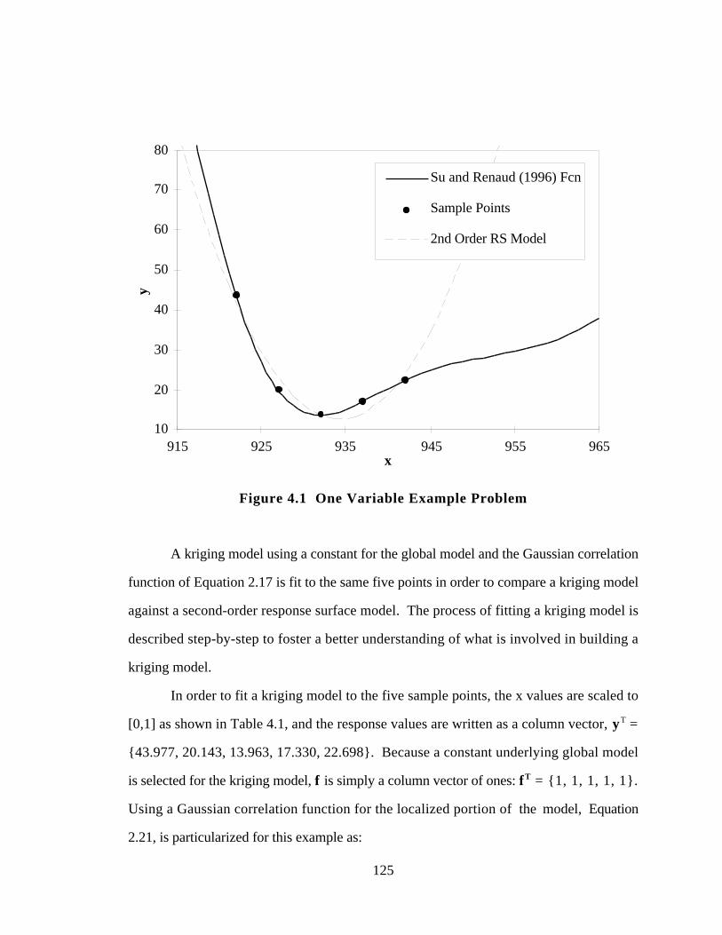
125
10
20
30
40
50
60
70
80
915 925 935 945 955 965x
y
Su and Renaud (1996) Fcn
Sample Points
2nd Order RS Model
Figure 4.1 One Variable Example Problem
A kriging model using a constant for the global model and the Gaussian correlation
function of Equation 2.17 is fit to the same five points in order to compare a kriging model
against a second-order response surface model. The process of fitting a kriging model is
described step-by-step to foster a better understanding of what is involved in building a
kriging model.
In order to fit a kriging model to the five sample points, the x values are scaled to
[0,1] as shown in Table 4.1, and the response values are written as a column vector, yT =
{43.977, 20.143, 13.963, 17.330, 22.698}. Because a constant underlying global model
is selected for the kriging model, f is simply a column vector of ones: fT = {1, 1, 1, 1, 1}.
Using a Gaussian correlation function for the localized portion of the model, Equation
2.21, is particularized for this example as:

126
R(x i,x j) = exp(−θ |x i − x j |2) i,j = 1,2,3,4,5;i ≠ j1 i = j
[4.2]
The correlation function for each sample point is then computed as follows:
i = 1, j = 1, R(x1,x1) = 1
i = 1, j = 2, R(x1,x2) = Exp(-θ|0.0 - 0.25|2) = exp(-0.0625θ)
i = 1, j = 3, R(x1,x3) = Exp(-θ|0.0 - 0.5|2) = exp(-0.25θ)
i = 1, j = 4, R(x1,x4) = Exp(-θ|0.0 - 0.75|2) = exp(-0.5625θ)
i = 1, j = 5, R(x1,x5) = Exp(-θ|0.0 - 1.0|2) = exp(-θ)
M
i = 5, j = 5, R(x5,x5) = 1
The resulting correlation matrix is thus:
R =
1 e−0.0625θ e−0.25 θ e−0.5625θ e− θ
1 e−0.0625θ e−0.25 θ e−0.5625θ
1 e− 0.0625θ e− 0.25θ
sym 1 e−0.0625θ
1
where θ is the unknown parameter which is used to fit the kriging model to the data.
The constant portion of the global model is now estimated using Equation 2.27
which is repeated here as Equation 4.3:
ˆ β = (f TR−1f)−1 fTR −1y [4.3]
and is a function of θ. The value for ˆ β , once the maximum likelihood estimate for θ is
known, is essentially a weighted average of the sample points based on intersite distances.
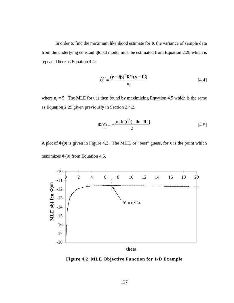
127
In order to find the maximum likelihood estimate for θ, the variance of sample data
from the underlying constant global model must be estimated from Equation 2.28 which is
repeated here as Equation 4.4:
ˆ σ 2 =(y − f ˆ β )T R−1(y − fˆ β )
ns
[4.4]
where ns = 5. The MLE for θ is then found by maximizing Equation 4.5 which is the same
as Equation 2.29 given previously in Section 2.4.2.
Φ(θ) = −[n s ln(ˆ σ 2) + ln | R |]
2[4.5]
A plot of Φ(θ) is given in Figure 4.2. The MLE, or “best” guess, for θ is the point which
maximizes Φ(θ) from Equation 4.5.
-18
-17
-16
-15
-14
-13
-12
-11
-100 2 4 6 8 10 12 14 16 18 20
theta
ML
E o
bj
fcn
θ* = 6.924
Φ(θ
)
Figure 4.2 MLE Objective Function for 1-D Example
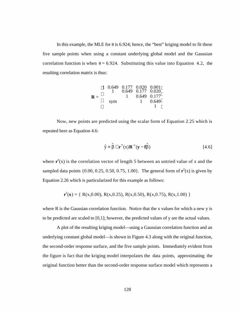
128
In this example, the MLE for θ is 6.924; hence, the “best” kriging model to fit these
five sample points when using a constant underlying global model and the Gaussian
correlation function is when θ = 6.924. Substituting this value into Equation 4.2, the
resulting correlation matrix is thus:
R =
1 0.649 0.177 0.020 0.0011 0.649 0.177 0.020
1 0.649 0.177sym 1 0.649
1
Now, new points are predicted using the scalar form of Equation 2.25 which is
repeated here as Equation 4.6:
ˆ y = ˆ β + rT(x)R−1(y − f ˆ β ) [4.6]
where rT(x) is the correlation vector of length 5 between an untried value of x and the
sampled data points {0.00, 0.25, 0.50, 0.75, 1.00}. The general form of rT(x) is given by
Equation 2.26 which is particularized for this example as follows:
rT(x) = { R(x,0.00), R(x,0.25), R(x,0.50), R(x,0.75), R(x,1.00) }
where R is the Gaussian correlation function. Notice that the x values for which a new y is
to be predicted are scaled to [0,1]; however, the predicted values of y are the actual values.
A plot of the resulting kriging model—using a Gaussian correlation function and an
underlying constant global model—is shown in Figure 4.3 along with the original function,
the second-order response surface, and the five sample points. Immediately evident from
the figure is fact that the kriging model interpolates the data points, approximating the
original function better than the second-order response surface model which represents a
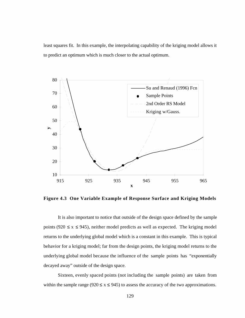
129
least squares fit. In this example, the interpolating capability of the kriging model allows it
to predict an optimum which is much closer to the actual optimum.
10
20
30
40
50
60
70
80
915 925 935 945 955 965x
y
Su and Renaud (1996) Fcn
Sample Points
2nd Order RS Model
Kriging w/Gauss.
Figure 4.3 One Variable Example of Response Surface and Kriging Models
It is also important to notice that outside of the design space defined by the sample
points (920 ≤ x ≤ 945), neither model predicts as well as expected. The kriging model
returns to the underlying global model which is a constant in this example. This is typical
behavior for a kriging model; far from the design points, the kriging model returns to the
underlying global model because the influence of the sample points has “exponentially
decayed away” outside of the design space.
Sixteen, evenly spaced points (not including the sample points) are taken from
within the sample range (920 ≤ x ≤ 945) to assess the accuracy of the two approximations.
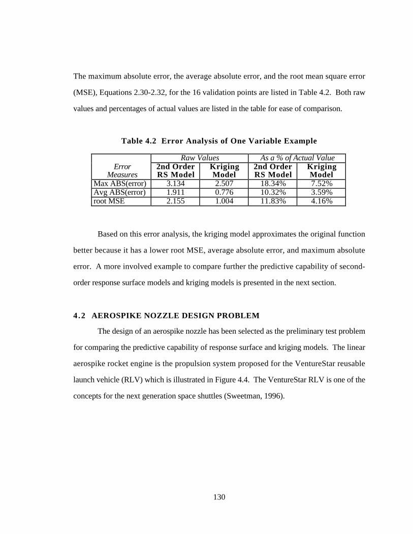
130
The maximum absolute error, the average absolute error, and the root mean square error
(MSE), Equations 2.30-2.32, for the 16 validation points are listed in Table 4.2. Both raw
values and percentages of actual values are listed in the table for ease of comparison.
Table 4.2 Error Analysis of One Variable Example
Raw Values As a % of Actual ValueError
Measures2nd OrderRS Model
KrigingModel
2nd OrderRS Model
KrigingModel
Max ABS(error) 3.134 2.507 18.34% 7.52%Avg ABS(error) 1.911 0.776 10.32% 3.59%root MSE 2.155 1.004 11.83% 4.16%
Based on this error analysis, the kriging model approximates the original function
better because it has a lower root MSE, average absolute error, and maximum absolute
error. A more involved example to compare further the predictive capability of second-
order response surface models and kriging models is presented in the next section.
4.2 AEROSPIKE NOZZLE DESIGN PROBLEM
The design of an aerospike nozzle has been selected as the preliminary test problem
for comparing the predictive capability of response surface and kriging models. The linear
aerospike rocket engine is the propulsion system proposed for the VentureStar reusable
launch vehicle (RLV) which is illustrated in Figure 4.4. The VentureStar RLV is one of the
concepts for the next generation space shuttles (Sweetman, 1996).
131
Figure 4.4 VentureStar RLV with Aerospike Nozzle (Korte, et al., 1997)
The aerospike rocket engine consists of a rocket thruster, cowl, aerospike nozzle,
and plug base regions as shown in Figure 4.5. The aerospike nozzle is a truncated spike or
plug nozzle that adjusts to the ambient pressure and integrates well with launch vehicles
(Rao, 1961). The flow field structure changes dramatically from low altitude to high
altitude on the spike surface and in the base region (Hagemann, et al., 1996; Mueller and
Sule, 1972; Rommel, et al., 1995). Additional flow is injected in the base region to create
an aerodynamic spike (Iacobellis, et al., 1967) which gives the aerospike nozzle its name
and increases the base pressure and contribution of the base region to the aerospike thrust.
Figure 4.5 Aerospike Components and Flow Field Characteristics(Korte, et al., 1997)
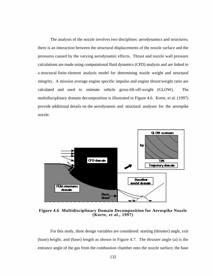
132
The analysis of the nozzle involves two disciplines: aerodynamics and structures;
there is an interaction between the structural displacements of the nozzle surface and the
pressures caused by the varying aerodynamic effects. Thrust and nozzle wall pressure
calculations are made using computational fluid dynamics (CFD) analysis and are linked to
a structural finite element analysis model for determining nozzle weight and structural
integrity. A mission average engine specific impulse and engine thrust/weight ratio are
calculated and used to estimate vehicle gross-lift-off-weight (GLOW). The
multidisciplinary domain decomposition is illustrated in Figure 4.6. Korte, et al. (1997)
provide additional details on the aerodynamic and structural analyses for the aerospike
nozzle.
Figure 4.6 Multidisciplinary Domain Decomposition for Aerospike Nozzle(Korte, et al., 1997)
For this study, three design variables are considered: starting (thruster) angle, exit
(base) height, and (base) length as shown in Figure 4.7. The thruster angle (a) is the
entrance angle of the gas from the combustion chamber onto the nozzle surface; the base
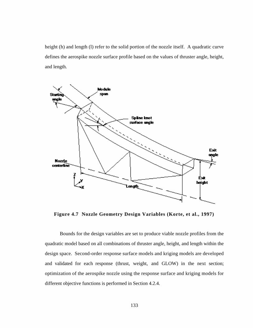
133
height (h) and length (l) refer to the solid portion of the nozzle itself. A quadratic curve
defines the aerospike nozzle surface profile based on the values of thruster angle, height,
and length.
Figure 4.7 Nozzle Geometry Design Variables (Korte, et al., 1997)
Bounds for the design variables are set to produce viable nozzle profiles from the
quadratic model based on all combinations of thruster angle, height, and length within the
design space. Second-order response surface models and kriging models are developed
and validated for each response (thrust, weight, and GLOW) in the next section;
optimization of the aerospike nozzle using the response surface and kriging models for
different objective functions is performed in Section 4.2.4.
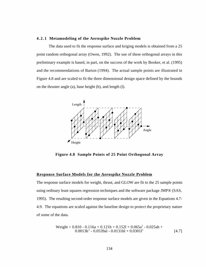
134
4 .2 .1 Metamodeling of the Aerospike Nozzle Problem
The data used to fit the response surface and kriging models is obtained from a 25
point random orthogonal array (Owen, 1992). The use of these orthogonal arrays in this
preliminary example is based, in part, on the success of the work by Booker, et al. (1995)
and the recommendations of Barton (1994). The actual sample points are illustrated in
Figure 4.8 and are scaled to fit the three dimensional design space defined by the bounds
on the thruster angle (a), base height (h), and length (l).
Angle
Height
Length
Figure 4.8 Sample Points of 25 Point Orthogonal Array
Response Surface Models for the Aerospike Nozzle Problem
The response surface models for weight, thrust, and GLOW are fit to the 25 sample points
using ordinary least squares regression techniques and the software package JMP® (SAS,
1995). The resulting second-order response surface models are given in the Equations 4.7-
4.9. The equations are scaled against the baseline design to protect the proprietary nature
of some of the data.
Weight = 0.810 - 0.116a + 0.121h + 0.152l + 0.065a2 - 0.025ah +0.0013h2 - 0.0539al - 0.0131hl + 0.0301l2 [4.7]
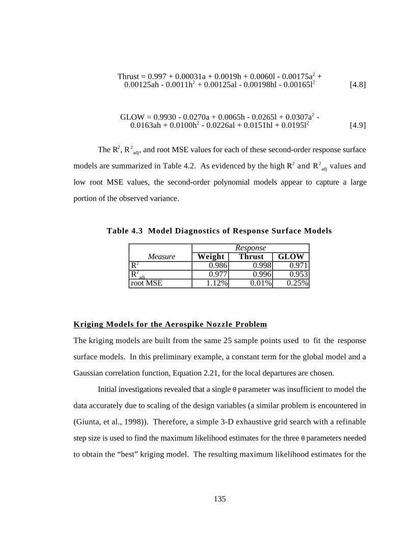
135
Thrust = 0.997 + 0.00031a + 0.0019h + 0.0060l - 0.00175a2 +0.00125ah - 0.0011h2 + 0.00125al - 0.00198hl - 0.00165l2 [4.8]
GLOW = 0.9930 - 0.0270a + 0.0065h - 0.0265l + 0.0307a2 -0.0163ah + 0.0100h2 - 0.0226al + 0.0151hl + 0.0195l2 [4.9]
The R2, R2adj, and root MSE values for each of these second-order response surface
models are summarized in Table 4.2. As evidenced by the high R2 and R2adj values and
low root MSE values, the second-order polynomial models appear to capture a large
portion of the observed variance.
Table 4.3 Model Diagnostics of Response Surface Models
ResponseMeasure Weight Thrust GLOW
R2 0.986 0.998 0.971R2
adj 0.977 0.996 0.953root MSE 1.12% 0.01% 0.25%
Kriging Models for the Aerospike Nozzle Problem
The kriging models are built from the same 25 sample points used to fit the response
surface models. In this preliminary example, a constant term for the global model and a
Gaussian correlation function, Equation 2.21, for the local departures are chosen.
Initial investigations revealed that a single θ parameter was insufficient to model the
data accurately due to scaling of the design variables (a similar problem is encountered in
(Giunta, et al., 1998)). Therefore, a simple 3-D exhaustive grid search with a refinable
step size is used to find the maximum likelihood estimates for the three θ parameters needed
to obtain the “best” kriging model. The resulting maximum likelihood estimates for the

136
three θ parameters for the weight, thrust, and GLOW models are summarized in Table 4.4;
note that these values are for the scaled sample points.
Table 4.4 Theta Parameters for Kriging Models of Aerospike Nozzle
MLE ResponseValues Weight Thrust GLOW
θangle = 0.548 0.30 3.362θheight = 1.323 0.50 2.437θlength = 2.718 0.65 0.537
With these parameters for the Gaussian correlation function, the kriging models
now are specified fully. A new point is predicted using these θ values and the 25 sample
points as shown in combination with Equations 2.25-2.27. The accuracy of the response
surface and kriging models is examined in the next two sections.
4 .2 .2 Error Analysis of Response Surface and Kriging Models
An additional 25 randomly selected validation points are used to verify the accuracy
of the response surface and kriging models. Error is defined as the difference between the
actual response from the computer analysis, y(x), and the predicted value, ˆ y (x), from the
response surface or kriging model. The maximum absolute error, the average absolute
error, and the root MSE, see Equations 2.30-2.32, for the 25 randomly selected validation
points are summarized in Table 4.5.
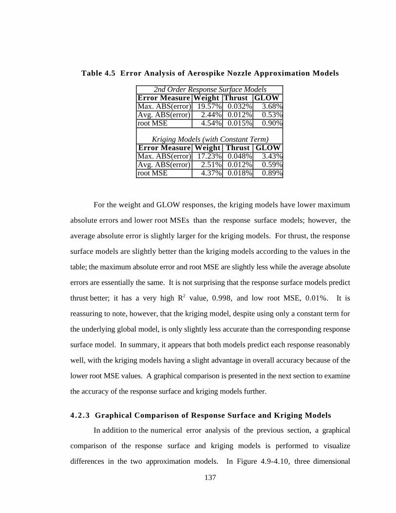
137
Table 4.5 Error Analysis of Aerospike Nozzle Approximation Models
2nd Order Response Surface ModelsError Measure Weight Thrust GLOWMax. ABS(error) 19.57% 0.032% 3.68%Avg. ABS(error) 2.44% 0.012% 0.53%root MSE 4.54% 0.015% 0.90%
Kriging Models (with Constant Term)Error Measure Weight Thrust GLOWMax. ABS(error) 17.23% 0.048% 3.43%Avg. ABS(error) 2.51% 0.012% 0.59%root MSE 4.37% 0.018% 0.89%
For the weight and GLOW responses, the kriging models have lower maximum
absolute errors and lower root MSEs than the response surface models; however, the
average absolute error is slightly larger for the kriging models. For thrust, the response
surface models are slightly better than the kriging models according to the values in the
table; the maximum absolute error and root MSE are slightly less while the average absolute
errors are essentially the same. It is not surprising that the response surface models predict
thrust better; it has a very high R2 value, 0.998, and low root MSE, 0.01%. It is
reassuring to note, however, that the kriging model, despite using only a constant term for
the underlying global model, is only slightly less accurate than the corresponding response
surface model. In summary, it appears that both models predict each response reasonably
well, with the kriging models having a slight advantage in overall accuracy because of the
lower root MSE values. A graphical comparison is presented in the next section to examine
the accuracy of the response surface and kriging models further.
4 .2 .3 Graphical Comparison of Response Surface and Kriging Models
In addition to the numerical error analysis of the previous section, a graphical
comparison of the response surface and kriging models is performed to visualize
differences in the two approximation models. In Figure 4.9-4.10, three dimensional
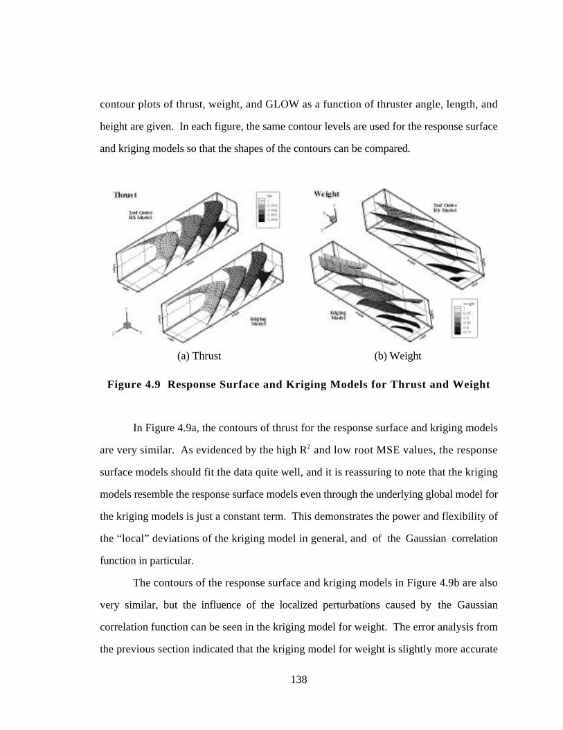
138
contour plots of thrust, weight, and GLOW as a function of thruster angle, length, and
height are given. In each figure, the same contour levels are used for the response surface
and kriging models so that the shapes of the contours can be compared.
(a) Thrust (b) Weight
Figure 4.9 Response Surface and Kriging Models for Thrust and Weight
In Figure 4.9a, the contours of thrust for the response surface and kriging models
are very similar. As evidenced by the high R2 and low root MSE values, the response
surface models should fit the data quite well, and it is reassuring to note that the kriging
models resemble the response surface models even through the underlying global model for
the kriging models is just a constant term. This demonstrates the power and flexibility of
the “local” deviations of the kriging model in general, and of the Gaussian correlation
function in particular.
The contours of the response surface and kriging models in Figure 4.9b are also
very similar, but the influence of the localized perturbations caused by the Gaussian
correlation function can be seen in the kriging model for weight. The error analysis from
the previous section indicated that the kriging model for weight is slightly more accurate
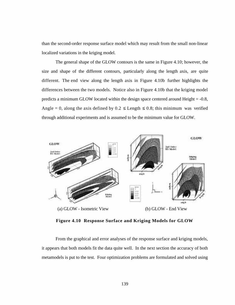
139
than the second-order response surface model which may result from the small non-linear
localized variations in the kriging model.
The general shape of the GLOW contours is the same in Figure 4.10; however, the
size and shape of the different contours, particularly along the length axis, are quite
different. The end view along the length axis in Figure 4.10b further highlights the
differences between the two models. Notice also in Figure 4.10b that the kriging model
predicts a minimum GLOW located within the design space centered around Height = -0.8,
Angle = 0, along the axis defined by 0.2 ≤ Length ≤ 0.8; this minimum was verified
through additional experiments and is assumed to be the minimum value for GLOW.
(a) GLOW - Isometric View (b) GLOW - End View
Figure 4.10 Response Surface and Kriging Models for GLOW
From the graphical and error analyses of the response surface and kriging models,
it appears that both models fit the data quite well. In the next section the accuracy of both
metamodels is put to the test. Four optimization problems are formulated and solved using
140
each of the metamodels and the efficiency and accuracy of the results are compared as a
final test of model adequacy.
4 .2 .4 Optimization using the Response Surface and Kriging Metamodels
The true test of the accuracy of the response surface and kriging models comes
when the approximations are used during optimization. It is paramount that any
approximations used in optimization prove reasonably accurate, lest they lead the
optimization algorithm into regions of bad designs. Trust Region approaches (see e.g.,
Lewis, 1996; Rodriguez, et al., 1997) and the Model Management framework (see e.g.,
Alexandrov, et al., 1997; Booker, et al., 1995) have been developed to ensure that
optimization algorithms are not led astray by inaccurate approximations. In this work,
however, the focus has been on developing the approximation models, particularly the
kriging models, and not on the optimization itself.
Four different optimization problems are formulated and solved to compare the
accuracy of the response surface and kriging models, see Table 4.6: (1) maximize thrust,
(2) minimize weight, (3) minimize GLOW, and (4) maximize thrust/weight ratio. The first
two objective functions in Table 4.6 represent traditional single objective, single discipline
optimization problems. The second two objective functions are more characteristic of
multidisciplinary optimization; minimizing GLOW or maximizing the thrust/weight ratio
requires tradeoffs between the aerodynamics and structures disciplines. As seen in the
table, for each objective function, constraint limits are placed on the remaining responses;
for instance, constraints are placed on the maximum allowable weight and GLOW and the
minimum allowable thrust/weight ratio when maximizing thrust. However, none of the
constraints are active in any of the final results.
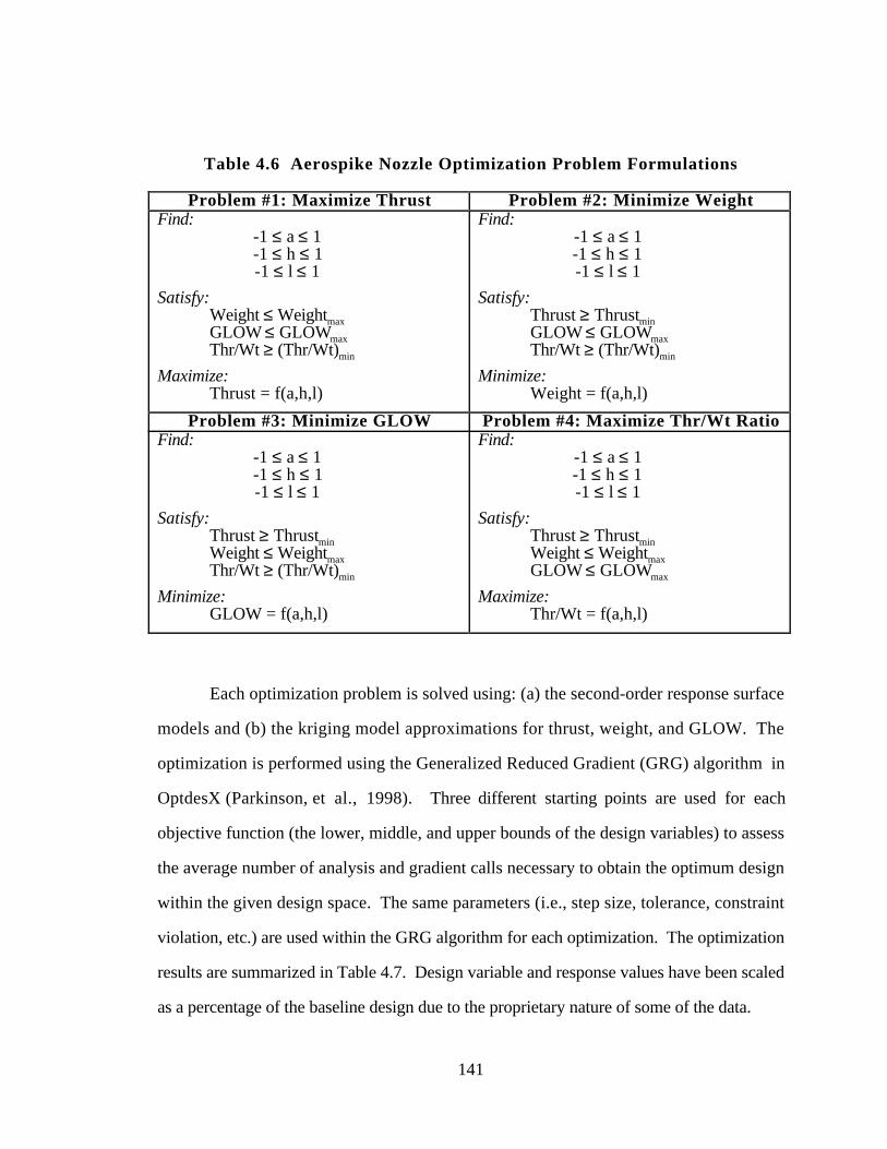
141
Table 4.6 Aerospike Nozzle Optimization Problem Formulations
Problem #1: Maximize Thrust Problem #2: Minimize WeightFind:
-1 ≤ a ≤ 1-1 ≤ h ≤ 1-1 ≤ l ≤ 1
Satisfy:Weight ≤ WeightmaxGLOW ≤ GLOWmaxThr/Wt ≥ (Thr/Wt)min
Maximize:Thrust = f(a,h,l)
Find:-1 ≤ a ≤ 1-1 ≤ h ≤ 1-1 ≤ l ≤ 1
Satisfy:Thrust ≥ ThrustminGLOW ≤ GLOWmaxThr/Wt ≥ (Thr/Wt)min
Minimize:Weight = f(a,h,l)
Problem #3: Minimize GLOW Problem #4: Maximize Thr/Wt RatioFind:
-1 ≤ a ≤ 1-1 ≤ h ≤ 1-1 ≤ l ≤ 1
Satisfy:Thrust ≥ ThrustminWeight ≤ WeightmaxThr/Wt ≥ (Thr/Wt)min
Minimize:GLOW = f(a,h,l)
Find:-1 ≤ a ≤ 1-1 ≤ h ≤ 1-1 ≤ l ≤ 1
Satisfy:Thrust ≥ ThrustminWeight ≤ WeightmaxGLOW ≤ GLOWmax
Maximize:Thr/Wt = f(a,h,l)
Each optimization problem is solved using: (a) the second-order response surface
models and (b) the kriging model approximations for thrust, weight, and GLOW. The
optimization is performed using the Generalized Reduced Gradient (GRG) algorithm in
OptdesX (Parkinson, et al., 1998). Three different starting points are used for each
objective function (the lower, middle, and upper bounds of the design variables) to assess
the average number of analysis and gradient calls necessary to obtain the optimum design
within the given design space. The same parameters (i.e., step size, tolerance, constraint
violation, etc.) are used within the GRG algorithm for each optimization. The optimization
results are summarized in Table 4.7. Design variable and response values have been scaled
as a percentage of the baseline design due to the proprietary nature of some of the data.
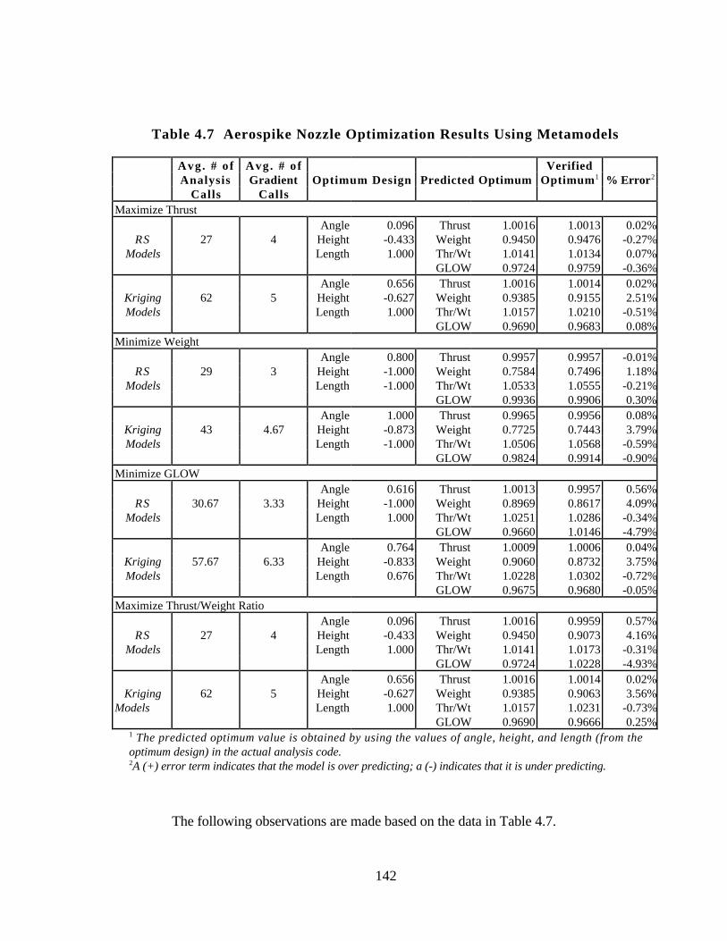
142
Table 4.7 Aerospike Nozzle Optimization Results Using Metamodels
Avg. # of Avg. # of VerifiedAnalysis Gradient Optimum Design Predicted Optimum Optimum1 % Error2
Calls CallsMaximize Thrust
Angle 0.096 Thrust 1.0016 1.0013 0.02%RS 27 4 Height -0.433 Weight 0.9450 0.9476 -0.27%
Models Length 1.000 Thr/Wt 1.0141 1.0134 0.07%GLOW 0.9724 0.9759 -0.36%
Angle 0.656 Thrust 1.0016 1.0014 0.02%Kriging 62 5 Height -0.627 Weight 0.9385 0.9155 2.51%Models Length 1.000 Thr/Wt 1.0157 1.0210 -0.51%
GLOW 0.9690 0.9683 0.08%Minimize Weight
Angle 0.800 Thrust 0.9957 0.9957 -0.01%RS 29 3 Height -1.000 Weight 0.7584 0.7496 1.18%
Models Length -1.000 Thr/Wt 1.0533 1.0555 -0.21%GLOW 0.9936 0.9906 0.30%
Angle 1.000 Thrust 0.9965 0.9956 0.08%Kriging 43 4.67 Height -0.873 Weight 0.7725 0.7443 3.79%Models Length -1.000 Thr/Wt 1.0506 1.0568 -0.59%
GLOW 0.9824 0.9914 -0.90%Minimize GLOW
Angle 0.616 Thrust 1.0013 0.9957 0.56%RS 30.67 3.33 Height -1.000 Weight 0.8969 0.8617 4.09%
Models Length 1.000 Thr/Wt 1.0251 1.0286 -0.34%GLOW 0.9660 1.0146 -4.79%
Angle 0.764 Thrust 1.0009 1.0006 0.04%Kriging 57.67 6.33 Height -0.833 Weight 0.9060 0.8732 3.75%Models Length 0.676 Thr/Wt 1.0228 1.0302 -0.72%
GLOW 0.9675 0.9680 -0.05%Maximize Thrust/Weight Ratio
Angle 0.096 Thrust 1.0016 0.9959 0.57%RS 27 4 Height -0.433 Weight 0.9450 0.9073 4.16%
Models Length 1.000 Thr/Wt 1.0141 1.0173 -0.31%GLOW 0.9724 1.0228 -4.93%
Angle 0.656 Thrust 1.0016 1.0014 0.02%Kriging 62 5 Height -0.627 Weight 0.9385 0.9063 3.56%
Models Length 1.000 Thr/Wt 1.0157 1.0231 -0.73%GLOW 0.9690 0.9666 0.25%
1 The predicted optimum value is obtained by using the values of angle, height, and length (from theoptimum design) in the actual analysis code.2A (+) error term indicates that the model is over predicting; a (-) indicates that it is under predicting.
The following observations are made based on the data in Table 4.7.
143
• Average number of analysis and gradient calls: In general, the response surface
models require fewer analysis and gradient calls to achieve the optimum than the
kriging models do. This can be attributed, in part, to the fact that the response
surface models are simple second-order polynomials; the kriging models are more
complex, non-linear functions as evidenced in Figure 4.9 and Figure 4.10.
• Convergence rates: Although not shown in the table, optimization using the
response surface models tends to converge more quickly than when using kriging
models. This can be inferred from the number of gradient calls which is one to
three calls fewer for the response surface models than the kriging models.
• Optimum designs: The optimum designs obtained from the response surface and
kriging models are essentially the same for each objective function, indicating that
both approximations send the optimization algorithm in the same general direction.
The largest discrepancy is the length for the minimize GLOW optimization;
response surface models predict the optimum GLOW occurs at the upper bound on
length (+1) while the kriging models yield 0.676. This difference is evident from
Figure 4.10. Furthermore, it has been verified through additional experiments that
the GLOW value obtained using the kriging models is the actual minimum.
• Predicted optima and prediction errors: To check the accuracy of the predicted
optima, the optimum design values for angle, height, and length are used as inputs
into the original analysis codes and the percentage difference between the actual and
predicted values is computed. The prediction error is less than 5% for all cases and
is 0.5% or less in three quarters of the results, indicating close agreement between
the metamodels and the actual analyses.
4 .2 .5 Lessons Learned from the Aerospike Nozzle Example
In summary, the response surface and kriging approximations yield comparable
results with minimal difference in predictive capability. It is worth noting that the kriging
models perform as well as the second-order response surface models even though the
global portion of the kriging model is only a constant. This helps to verify
Hypothesis 2 which states that kriging models are a viable metamodeling
144
technique for building approximations of deterministic computer analyses;
however, many questions remain unanswered.
• Correlation function: A Gaussian correlation function is utilized in this example to
fit the data, but is this the best correlation function of the five being considered in
this dissertation?
• Experimental design: A 25 point random orthogonal array is used in this example
to sample the design space and provide data to fit both the kriging and response
surface models, but is this the best type of experimental design for sampling
deterministic computer codes such as the ones used in this example? Would an
alternative experimental design yield a more accurate predictor?
• Model validation: Because kriging models interpolate the data, R2 values and
residual plots cannot be used to assess model accuracy. In this example an
additional 25 validation points are employed to assess accuracy; however, other
validation approaches exist. One such approach which does not require additional
validation points is leave-one-out cross validation (Mitchell and Morris, 1992)
mentioned in Section 2.4.2. Does cross validation provide a sufficient assessment
of model accuracy?
A study of six engineering test problems is set up and performed in the next chapter to
answer these questions. In closing this chapter, a brief look ahead to that study is offered
in the next section.
4.3 A LOOK BACK AND A LOOK AHEAD
In an attempt to determine the types of applications for which kriging is useful,
several engineering examples are introduced in the next chapter to serve as test problems to
establish the utility of kriging and verify Hypothesis 2. In addition to testing Hypothesis 2,
several classical and space filling experimental designs are compared and contrasted in an
effort to test Hypothesis 3 to determine if space filling experimental designs are better
suited for building metamodels of deterministic computer experiments.

145
5. 5CHAPTER 5
THE UTILITY OF KRIGING AND SPACEFILLING EXPERIMENTAL DESIGNS
Kriging/DOE Testbed
In this chapter, Hypotheses 2 and 3 are tested explicitly, verifying the utility of
kriging and space filling experimental designs for building metamodels of deterministic
computer analyses. A pictorial overview and specific details of the study are given in
Section 5.1. Six engineering examples, introduced in Section 5.1.1, provide a testbed
of problems to benchmark kriging and space filling designs and verify
Hypotheses 2 and 3. In Sections 5.1.2, 5.1.3, and 5.1.4, the factors, experimental
designs, and responses in the study are explained. Analysis of variance of the data and
response correlation are presented in the precursory data analysis in Section 5.2. Section
5.3 contains the results of testing Hypothesis 2 and a discussion of the ramifications of the
results; the results and discussion regarding Hypothesis 3 follow in Section 5.4. A
summary of the study and its relevance to the development of the PPCEM is offered in
Section 5.5.
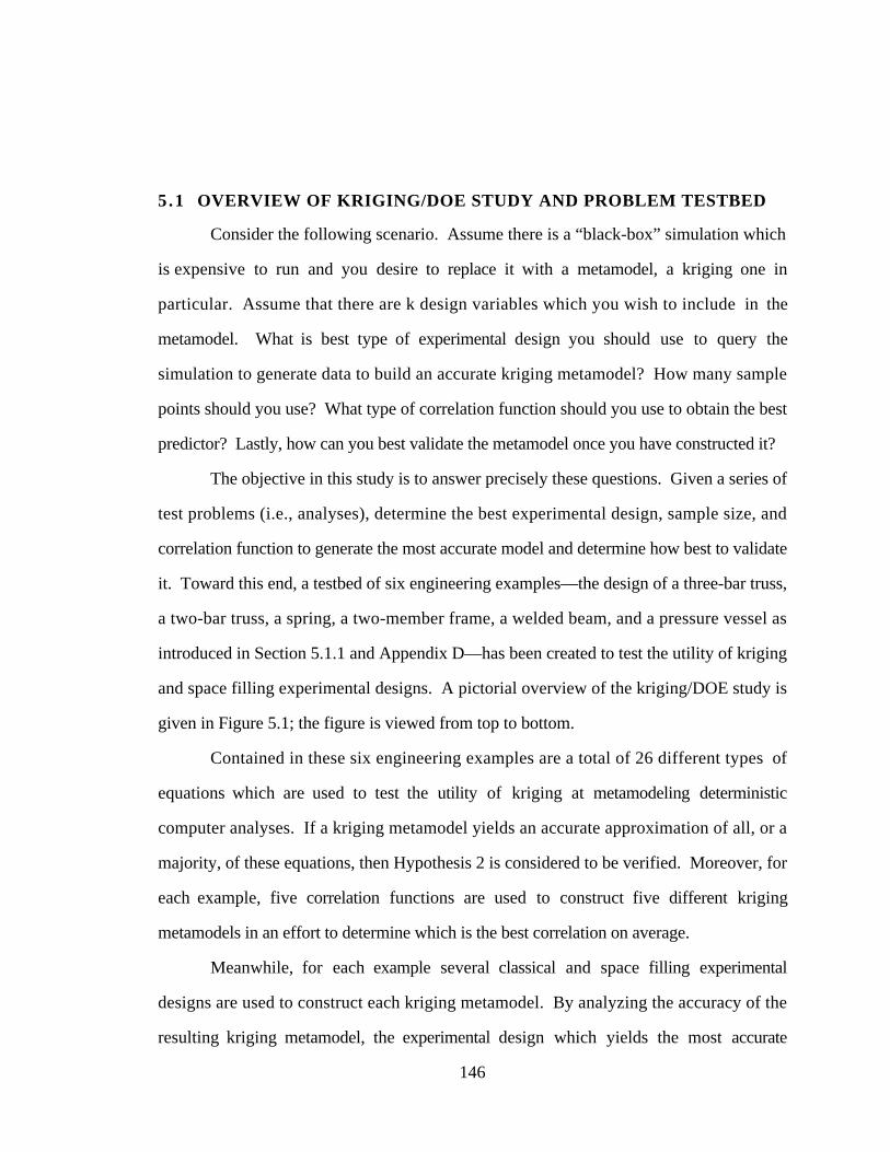
146
5.1 OVERVIEW OF KRIGING/DOE STUDY AND PROBLEM TESTBED
Consider the following scenario. Assume there is a “black-box” simulation which
is expensive to run and you desire to replace it with a metamodel, a kriging one in
particular. Assume that there are k design variables which you wish to include in the
metamodel. What is best type of experimental design you should use to query the
simulation to generate data to build an accurate kriging metamodel? How many sample
points should you use? What type of correlation function should you use to obtain the best
predictor? Lastly, how can you best validate the metamodel once you have constructed it?
The objective in this study is to answer precisely these questions. Given a series of
test problems (i.e., analyses), determine the best experimental design, sample size, and
correlation function to generate the most accurate model and determine how best to validate
it. Toward this end, a testbed of six engineering examples—the design of a three-bar truss,
a two-bar truss, a spring, a two-member frame, a welded beam, and a pressure vessel as
introduced in Section 5.1.1 and Appendix D—has been created to test the utility of kriging
and space filling experimental designs. A pictorial overview of the kriging/DOE study is
given in Figure 5.1; the figure is viewed from top to bottom.
Contained in these six engineering examples are a total of 26 different types of
equations which are used to test the utility of kriging at metamodeling deterministic
computer analyses. If a kriging metamodel yields an accurate approximation of all, or a
majority, of these equations, then Hypothesis 2 is considered to be verified. Moreover, for
each example, five correlation functions are used to construct five different kriging
metamodels in an effort to determine which is the best correlation on average.
Meanwhile, for each example several classical and space filling experimental
designs are used to construct each kriging metamodel. By analyzing the accuracy of the
resulting kriging metamodel, the experimental design which yields the most accurate
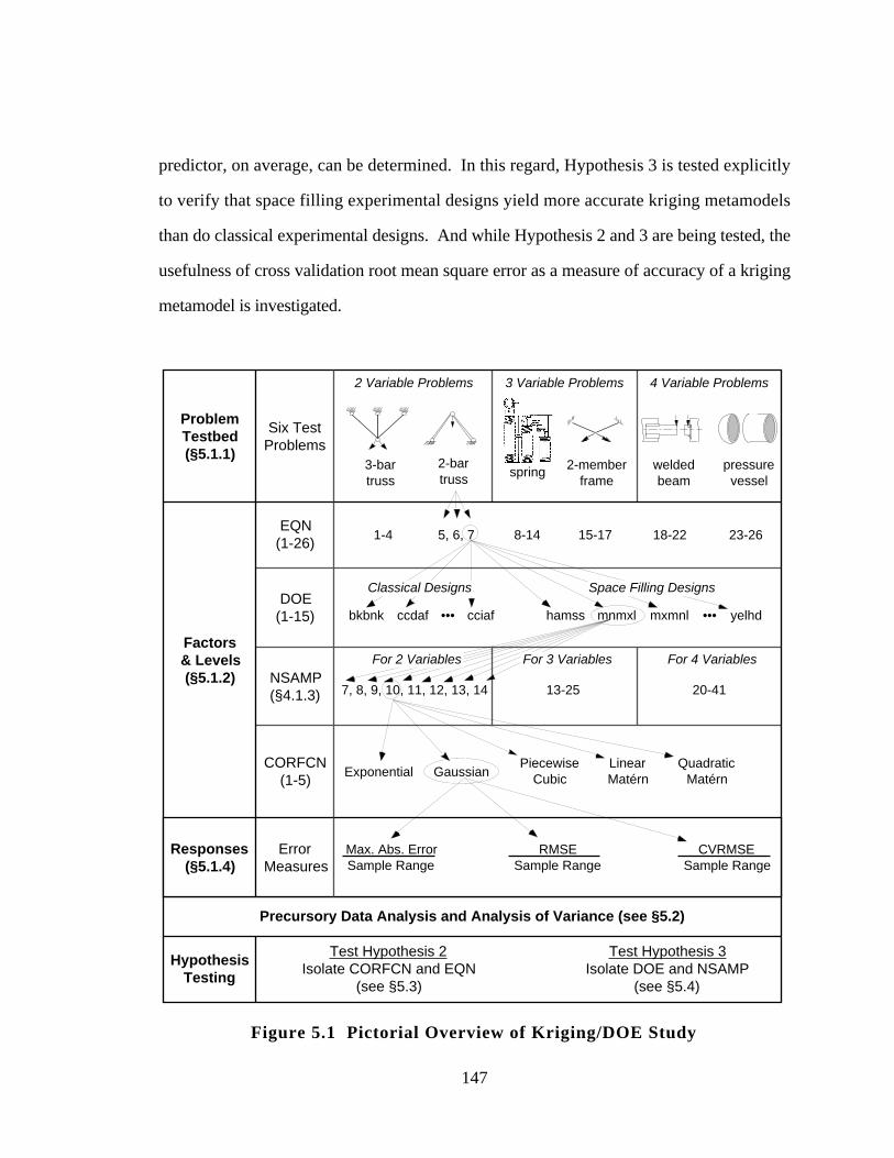
147
predictor, on average, can be determined. In this regard, Hypothesis 3 is tested explicitly
to verify that space filling experimental designs yield more accurate kriging metamodels
than do classical experimental designs. And while Hypothesis 2 and 3 are being tested, the
usefulness of cross validation root mean square error as a measure of accuracy of a kriging
metamodel is investigated.
ProblemTestbed(§5.1.1)
DOE(1-15)
CORFCN(1-5)
EQN(1-26)
NSAMP(§4.1.3)
3-bartruss
2-bartruss
2 Variable Problems
2-memberframe
spring
3 Variable Problems
weldedbeam
pressurevessel
4 Variable Problems
Factors& Levels(§5.1.2)
Responses(§5.1.4)
1-4 5, 6, 7 8-14 15-17 18-22 23-26
ccdaf •••bkbnk cciaf mnmxlhamss yelhd•••
Test Hypothesis 2Isolate CORFCN and EQN
(see §5.3)
Test Hypothesis 3Isolate DOE and NSAMP
(see §5.4)
mxmnl
7, 8, 9, 10, 11, 12, 13, 14
Exponential GaussianPiecewise
CubicLinearMatérn
QuadraticMatérn
13-25 20-41
Max. Abs. ErrorSample Range
RMSESample Range
CVRMSESample Range
Space Filling DesignsClassical Designs
Six TestProblems
ErrorMeasures
HypothesisTesting
For 2 Variables For 3 Variables For 4 Variables
Precursory Data Analysis and Analysis of Variance (see §5.2)
Figure 5.1 Pictorial Overview of Kriging/DOE Study

148
In total, 7905 kriging models are constructed: one for each correlation function
(CORFCN) for each experimental design (DOE) for each sample size (NSAMP) for each
equation (EQN) in each problem. As an example, the arrows in Figure 5.1 trace Equation
7 in the two-bar truss problem. For EQN 7, there are 15 possible experimental design
(DOE) choices; in this case, the minimax Latin hypercube design (mnmxl) is being
considered. For this design, there are several possible choices for NSAMP, ranging from
7-14, because this is a two variable problem. Using 10 sample points as an example, at the
next level there are five correlation functions (CORFCN) which can be used to build a
kriging model; the Gaussian correlation function is highlighted in this example. Finally,
three measures of model accuracy are computed for the kriging model resulting from this
particular combination of EQN, DOE, NSAMP, and CORFCN: max. abs. error, root mean
square error (RMSE), and cross validation root mean square error (CVRMSE) which are
“normalized” by the corresponding sample range so that responses of different magnitude
can be compared directly.
After a precursory analysis of the data in Section 5.2, these three error measures of
model accuracy are used to test Hypotheses 2 and 3 explicitly. As shown in Figure 5.1:
Hypothesis 2 is tested in Section 5.3 by isolating the effects of correlation function
(CORFCN) and equation (EQN) on the accuracy of the resulting kriging model as
assessed through the error measures.
Hypothesis 3 is tested in Section 5.4 by isolating the effects of experimental design
(DOE) and sample size (NSAMP) on the error measures of accuracy of the resulting
kriging model.
The test problems used in this study are introduced next.
5 .1 .1 Overview of Testbed Problems
Six test problems were selected from the literature to provide a testbed for assessing
the utility of kriging and several different space filling experimental designs. These
149
problems are not meant to be all inclusive; rather, they are taken as representative of typical
analyses encountered in mechanical design. The analysis of these problems is simple
enough not to warrant building kriging models of the responses; however, these problems
have been selected because:
a. they have been well studied and the behavior of the system and the underlying
analysis equations are known,
b. the corresponding “region of interest” is known in each problem, and
c. they have been used by other researchers to test their own metamodeling strategies
and algorithms.
Furthermore, the optimum solution for each problem is also known; however, a more
extensive error analysis is employed to assess the accuracy of the kriging models (see
Section 5.1.4).
In the following sections, each example is described along with its pertinent
constraints, design variable bounds, and the objective function; note that a kriging model is
constructed for each constraint and objective function in each problem. The values of the
parameters in the equations (i.e., all of the letters and symbols which are not explicitly
stated as being design variables) are given in the referenced sections of Appendix D which
contain the complete description of each problem.
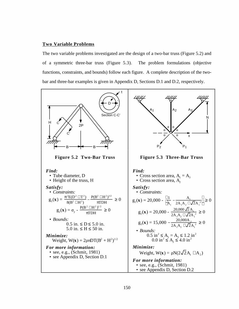
150
Two Variable Problems
The two variable problems investigated are the design of a two-bar truss (Figure 5.2) and
of a symmetric three-bar truss (Figure 5.3). The problem formulations (objective
functions, constraints, and bounds) follow each figure. A complete description of the two-
bar and three-bar examples is given in Appendix D, Sections D.1 and D.2, respectively.
t
D
Section C-C’
H2P
B B
C
C’
N
x
P1P2
αααα
αα
A1 A2 A3
Figure 5.2 Two-Bar Truss
Find:• Tube diameter, D• Height of the truss, H
Satisfy:• Constraints:
g1(x) = π 2E(D 2 + T 2 )
8(B2 + H 2 )−
P(B2 + H 2 )1/2
πTDH ≥ 0
g2(x) = σy - P(B 2 + H 2 )1/2
πTDH ≥ 0
• Bounds: 0.5 in. ≤ D ≤ 5.0 in.5.0 in. ≤ H ≤ 50 in.
Minimize:Weight, W(x) = 2ρπDT(B2 + H2)1/2
For more information:• see, e.g., (Schmit, 1981)• see Appendix D, Section D.1
Figure 5.3 Three-Bar Truss
Find:• Cross section area, A1 = A3• Cross section area, A2
Satisfy:• Constraints:
g1(x) = 20,000 - 1
A1
−A2
2A 1A 2 + 2A 12
≥ 0
g2(x) = 20,000 - 20,000 2 A1
2A 1A2 + 2A 12 ≥ 0
g3(x) = 15,000 −20,000A 2
2A 1A2 + 2A12 ≥ 0
• Bounds:0.5 in2 ≤ A1 = A3 ≤ 1.2 in2
0.0 in2 ≤ A2 ≤ 4.0 in2
Minimize:Weight, W(x) = ρN(2 2A1 + A2)
For more information:• see, e.g., (Schmit, 1981)• see Appendix D, Section D.2
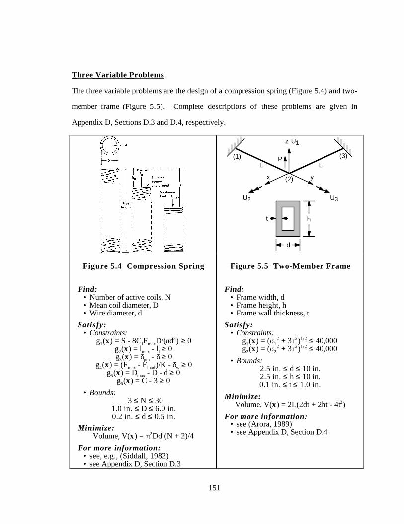
151
Three Variable Problems
The three variable problems are the design of a compression spring (Figure 5.4) and two-
member frame (Figure 5.5). Complete descriptions of these problems are given in
Appendix D, Sections D.3 and D.4, respectively.
ht
d
(1)
(2)
(3)LL
z
P
x y
U1
U2 U3
Figure 5.4 Compression Spring
Find:• Number of active coils, N• Mean coil diameter, D• Wire diameter, d
Satisfy:• Constraints:
g1(x) = S - 8CfFmaxD/(πd3) ≥ 0g2(x) = lmax - lf ≥ 0g3(x) = δpm - δ ≥ 0
g4(x) = (Fmax - Fload)/K - δw ≥ 0g5(x) = Dmax - D - d ≥ 0
g6(x) = C - 3 ≥ 0
• Bounds: 3 ≤ N ≤ 30
1.0 in. ≤ D ≤ 6.0 in.0.2 in. ≤ d ≤ 0.5 in.
Minimize:Volume, V(x) = π2Dd2(N + 2)/4
For more information:• see, e.g., (Siddall, 1982)• see Appendix D, Section D.3
Figure 5.5 Two-Member Frame
Find:• Frame width, d• Frame height, h• Frame wall thickness, t
Satisfy:• Constraints:
g1(x) = (σ12 + 3τ2)1/2 ≤ 40,000
g2(x) = (σ22 + 3τ2)1/2 ≤ 40,000
• Bounds:2.5 in. ≤ d ≤ 10 in.2.5 in. ≤ h ≤ 10 in.0.1 in. ≤ t ≤ 1.0 in.
Minimize:Volume, V(x) = 2L(2dt + 2ht - 4t2)
For more information:• see (Arora, 1989)• see Appendix D, Section D.4
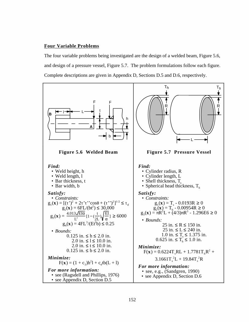
152
Four Variable Problems
The four variable problems being investigated are the design of a welded beam, Figure 5.6,
and design of a pressure vessel, Figure 5.7. The problem formulations follow each figure.
Complete descriptions are given in Appendix D, Sections D.5 and D.6, respectively.
B
A
L
F
h
F
b
l tR
TsTh
R
L
Figure 5.6 Welded Beam
Find:• Weld height, h• Weld length, l• Bar thickness, t• Bar width, b
Satisfy:• Constraints:
g1(x) = [(τ’)2 + 2τ’τ’’cosθ + (τ’’)2]1/2 ≤ τdg2(x) = 6FL/(bt2) ≤ 30,000
g3(x) = 4.013 EIα
L2 [1− (t
2L)
EI
α] ≥ 6000
g4(x) = 4FL3/(Et3b) ≤ 0.25
• Bounds:0.125 in. ≤ h ≤ 2.0 in. 2.0 in. ≤ l ≤ 10.0 in. 2.0 in. ≤ t ≤ 10.0 in.0.125 in. ≤ b ≤ 2.0 in.
Minimize:F(x) = (1 + c3)h
2l + c4tb(L + l)
For more information:• see (Ragsdell and Phillips, 1976)• see Appendix D, Section D.5
Figure 5.7 Pressure Vessel
Find:• Cylinder radius, R• Cylinder length, L• Shell thickness, Ts• Spherical head thickness, Th
Satisfy:• Constraints:
g1(x) = Ts - 0.0193R ≥ 0g2(x) = Th - 0.00954R ≥ 0
g3(x) = πR2L + (4/3)πR3 - 1.296E6 ≥ 0
• Bounds: 25 in. ≤ R ≤ 150 in. 25 in. ≤ L ≤ 240 in.
1.0 in. ≤ Ts ≤ 1.375 in.0.625 in. ≤ Th ≤ 1.0 in.
Minimize:F(x) = 0.6224T sRL + 1.7781ThR
2 +
3.1661Ts2L + 19.84Ts
2R
For more information:• see, e.g., (Sandgren, 1990)• see Appendix D, Section D.6
153
Taken together, these six problems provide a wide variety of functions to
approximate since a kriging model is built for each objective function and constraint for
each problem. In total, there are 26 different equations contained in these six problems,
ranging from simple linear functions to reciprocal square roots; some equations even
require the inversion of a finite element matrix (see Section D.4 for the analysis of the two-
member frame). With these six problems as the testbed for verifying Hypotheses 2 and 3,
the factors (and corresponding levels of interest) being studied are explained next.
5 .1 .2 Factors and Levels for Kriging/DOE Experiment
The three basic factors considered in this experiment are listed in Table 5.1:
CORFCN refers to the correlation function used in the kriging model, EQN refers to the
equation being approximated, and DOE refers to the type of experimental design being
utilized to sample the equation to provide data to fit the model. The corresponding levels
for each factor also are listed in the table and are explained as follows.
• CORFCN has 5 levels of interest based on the correlation functions being studied
(refer to Table 2.1, Equations 2.20-2.24); the correlation function associated with
each level is given in the first two columns of Table 5.1.
• EQN has 26 levels based on the total number of equations (i.e., objective functions
and constraints) in the six test problems; when showing the levels for EQN, the
objective function for each problem is singled out from the constraints, see the
middle two columns of Table 5.1.
• DOE has 15 levels based on all of the classical and space filling experimental design
introduced in Section 2.4.3 for investigation; the acronyms and corresponding
name of each design is listed in the last two columns of Table 5.1.
Every effort is made to ensure that the observations of each factor level in the
experiment are properly balanced; however, some factors (and levels) are beyond control.
Each level of CORFCN given in Table 5.1 occurs an equal number of times in each
problem; hence, it is easy to examine the effect of the different correlation functions on the
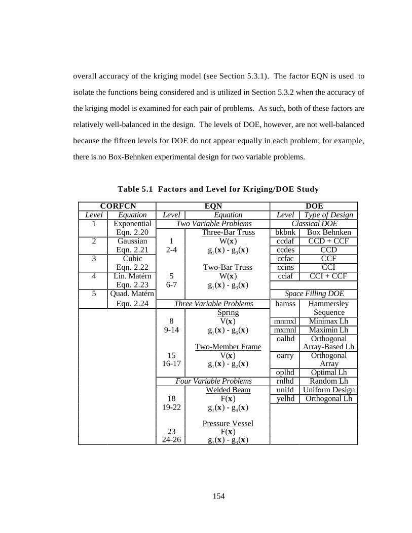
154
overall accuracy of the kriging model (see Section 5.3.1). The factor EQN is used to
isolate the functions being considered and is utilized in Section 5.3.2 when the accuracy of
the kriging model is examined for each pair of problems. As such, both of these factors are
relatively well-balanced in the design. The levels of DOE, however, are not well-balanced
because the fifteen levels for DOE do not appear equally in each problem; for example,
there is no Box-Behnken experimental design for two variable problems.
Table 5.1 Factors and Level for Kriging/DOE Study
CORFCN EQN DOELevel Equation Level Equation Level Type of Design
1 Exponential Two Variable Problems Classical DOEEqn. 2.20 Three-Bar Truss bkbnk Box Behnken
2 Gaussian 1 W(x) ccdaf CCD + CCFEqn. 2.21 2-4 g1(x) - g3(x) ccdes CCD
3 Cubic ccfac CCFEqn. 2.22 Two-Bar Truss ccins CCI
4 Lin. Matérn 5 W(x) cciaf CCI + CCFEqn. 2.23 6-7 g1(x) - g3(x)
5 Quad. Matérn Space Filling DOEEqn. 2.24 Three Variable Problems hamss Hammersley
Spring Sequence8 V(x) mnmxl Minimax Lh
9-14 g1(x) - g6(x) mxmnl Maximin Lhoalhd Orthogonal
Two-Member Frame Array-Based Lh15 V(x) oarry Orthogonal
16-17 g1(x) - g2(x) Arrayoplhd Optimal Lh
Four Variable Problems rnlhd Random Lh Welded Beam unifd Uniform Design
18 F(x) yelhd Orthogonal Lh19-22 g1(x) - g4(x)
Pressure Vessel 23 F(x)
24-26 g1(x) - g3(x)
155
To make things even more complicated, the number of sample points within each
design depends on the type of DOE considered and the number of variables in the problem.
For instance, a CCD for the two variable problems has 22 + 2•2 + 1 = 9 points while a
random Latin hypercube can have any number of sample points. Hence, great care must be
taken when analyzing the effects of DOE because of the biasing which occurs due to
unbalanced sample sizes in the experiment. This is discussed in more detail in the next
section which contains a complete listing of which experimental designs (and
corresponding sample sizes) are used in each of the two, three, and four variable problems.
5 .1 .3 Experimental Design Choices for Test Problems
A very important factor in the selection of an experimental design is the number of
points used. How is the number of points to be determined for a given design? For the
two types of classical designs utilized in this dissertation—CCDs and Box-Behnken
designs—the number of points essentially is fixed once the number of factors is specified.
Fractional factorial designs within a CCD are not considered for these problems because
they contain so few variables. Unlike the CCDs and Box-Behnken designs, for most space
filling designs the number of points is not dictated by the number of factors and can be any
number within reason.
Therefore, in order to determine the number of points used in a space filling design,
a CCD with the same number of factors is used to determine the baseline number of points,
e.g., for three factors, a CCD requires 15 points, and the number of points used in all
space filling designs for three factors would be selected to be as close to 15 as possible.
However, because some space filling designs can have a variable number of sample points,
a variety of sample sizes for each design are considered in order to see if fewer or slightly
more points provides an improved fit. As a guideline, an upper bound on the number of
points of about 1.5 times the number prescribed by the baseline CCD is employed. This
156
factor of 1.5 is primarily based on the recommendations of Giunta, et al. (1994) who found
that for small problems (i.e., fewer than about five factors) the variance of a second-order
response surface model leveled off when the number of sample points was about 1.5 times
the number of terms in the polynomial model. This number serves as a guideline in this
work despite the fact that kriging models do not necessarily use a second-order polynomial.
How important is the number of design points when picking an experimental
design? The answer is very important. In order to compare the utility of different
experimental designs properly, it is important to use the same number of sample points
because a design with more sample points is expected to provide more information,
possibly resulting in a more accurate model. Therefore, when designs do not have the
same number of points, it is impossible to determine if an improvement in model accuracy
is from the design itself (i.e., spacing of the points in the design space) or from the number
of sample points. However, in some cases it is extremely difficult, if not impossible, to
have two different designs which have the same number of points. For instance, a three
factor CCD has 15 points, a three factor Box-Behnken has 13 (since replicates are not
used), and a strength 2 randomized OA has either 9, 16, or 25 points since it is restricted to
q2 points where q is the number of levels and is restricted to be a prime power. Despite
these difficulties, every effort is made to make the sample sizes overlap as much as possible
from one design to the next. The experimental designs and corresponding sample sizes for
each pair of problems are described in the following sections.
Two Variable Problems
For the two variable problems (the two-bar and three-bar trusses), nine types of
experimental designs are considered, see Table 5.2. Of these nine types of designs, there
are 51 unique designs because each design which has a different number of points is
considered a unique design. For instance, a seven point Latin hypercube and an eight point
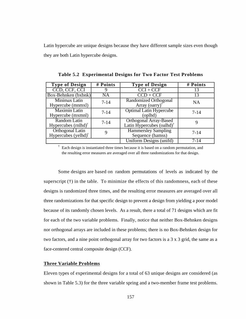
157
Latin hypercube are unique designs because they have different sample sizes even though
they are both Latin hypercube designs.
Table 5.2 Experimental Designs for Two Factor Test Problems
Type of Design # Points Type of Design # PointsCCD, CCF, CCI 9 CCI + CCF 13
Box-Behnken (bxbnk) NA CCD + CCF 13Minimax Latin
Hypercube (mnmxl)7-14 Randomized Orthogonal
Array (oarry)† NA
Maximin LatinHypercube (mxmnl)
7-14 Optimal Latin Hypercube(oplhd)
7-14
Random LatinHypercubes (rnlhd)† 7-14 Orthogonal Array-Based
Latin Hypercubes (oalhd)† 9
Orthogonal LatinHypercubes (yelhd)† 9 Hammersley Sampling
Sequence (hamss)7-14
Uniform Designs (unifd) 7-14† Each design is instantiated three times because it is based on a random permutation, and
the resulting error measures are averaged over all three randomizations for that design.
Some designs are based on random permutations of levels as indicated by the
superscript (†) in the table. To minimize the effects of this randomness, each of these
designs is randomized three times, and the resulting error measures are averaged over all
three randomizations for that specific design to prevent a design from yielding a poor model
because of its randomly chosen levels. As a result, there a total of 71 designs which are fit
for each of the two variable problems. Finally, notice that neither Box-Behnken designs
nor orthogonal arrays are included in these problems; there is no Box-Behnken design for
two factors, and a nine point orthogonal array for two factors is a 3 x 3 grid, the same as a
face-centered central composite design (CCF).
Three Variable Problems
Eleven types of experimental designs for a total of 63 unique designs are considered (as
shown in Table 5.3) for the three variable spring and a two-member frame test problems.
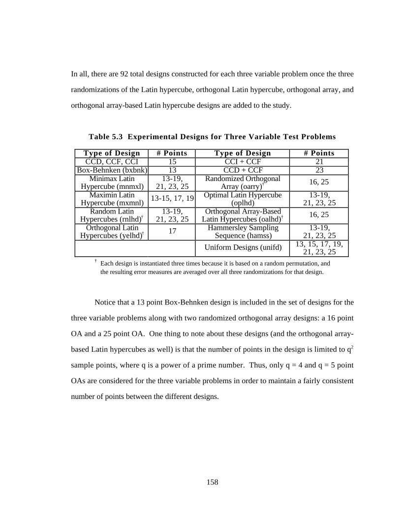
158
In all, there are 92 total designs constructed for each three variable problem once the three
randomizations of the Latin hypercube, orthogonal Latin hypercube, orthogonal array, and
orthogonal array-based Latin hypercube designs are added to the study.
Table 5.3 Experimental Designs for Three Variable Test Problems
Type of Design # Points Type of Design # PointsCCD, CCF, CCI 15 CCI + CCF 21
Box-Behnken (bxbnk) 13 CCD + CCF 23Minimax Latin
Hypercube (mnmxl)13-19,
21, 23, 25Randomized Orthogonal
Array (oarry)† 16, 25
Maximin LatinHypercube (mxmnl)
13-15, 17, 19 Optimal Latin Hypercube(oplhd)
13-19,21, 23, 25
Random LatinHypercubes (rnlhd)†
13-19,21, 23, 25
Orthogonal Array-BasedLatin Hypercubes (oalhd)† 16, 25
Orthogonal LatinHypercubes (yelhd)† 17 Hammersley Sampling
Sequence (hamss)13-19,
21, 23, 25
Uniform Designs (unifd) 13, 15, 17, 19,21, 23, 25
† Each design is instantiated three times because it is based on a random permutation, andthe resulting error measures are averaged over all three randomizations for that design.
Notice that a 13 point Box-Behnken design is included in the set of designs for the
three variable problems along with two randomized orthogonal array designs: a 16 point
OA and a 25 point OA. One thing to note about these designs (and the orthogonal array-
based Latin hypercubes as well) is that the number of points in the design is limited to q2
sample points, where q is a power of a prime number. Thus, only q = 4 and q = 5 point
OAs are considered for the three variable problems in order to maintain a fairly consistent
number of points between the different designs.
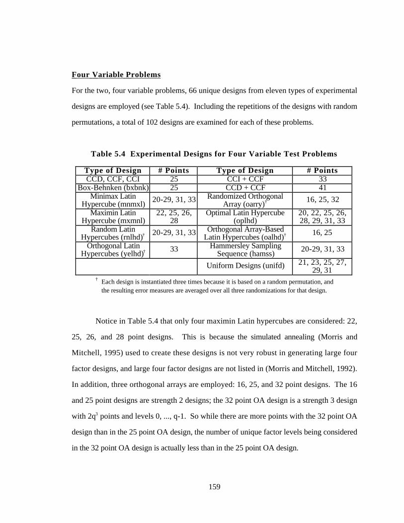
159
Four Variable Problems
For the two, four variable problems, 66 unique designs from eleven types of experimental
designs are employed (see Table 5.4). Including the repetitions of the designs with random
permutations, a total of 102 designs are examined for each of these problems.
Table 5.4 Experimental Designs for Four Variable Test Problems
Type of Design # Points Type of Design # PointsCCD, CCF, CCI 25 CCI + CCF 33
Box-Behnken (bxbnk) 25 CCD + CCF 41Minimax Latin
Hypercube (mnmxl)20-29, 31, 33 Randomized Orthogonal
Array (oarry)† 16, 25, 32
Maximin LatinHypercube (mxmnl)
22, 25, 26,28
Optimal Latin Hypercube(oplhd)
20, 22, 25, 26,28, 29, 31, 33
Random LatinHypercubes (rnlhd)† 20-29, 31, 33 Orthogonal Array-Based
Latin Hypercubes (oalhd)† 16, 25
Orthogonal LatinHypercubes (yelhd)† 33 Hammersley Sampling
Sequence (hamss)20-29, 31, 33
Uniform Designs (unifd) 21, 23, 25, 27,29, 31
† Each design is instantiated three times because it is based on a random permutation, andthe resulting error measures are averaged over all three randomizations for that design.
Notice in Table 5.4 that only four maximin Latin hypercubes are considered: 22,
25, 26, and 28 point designs. This is because the simulated annealing (Morris and
Mitchell, 1995) used to create these designs is not very robust in generating large four
factor designs, and large four factor designs are not listed in (Morris and Mitchell, 1992).
In addition, three orthogonal arrays are employed: 16, 25, and 32 point designs. The 16
and 25 point designs are strength 2 designs; the 32 point OA design is a strength 3 design
with 2q3 points and levels 0, ..., q-1. So while there are more points with the 32 point OA
design than in the 25 point OA design, the number of unique factor levels being considered
in the 32 point OA design is actually less than in the 25 point OA design.
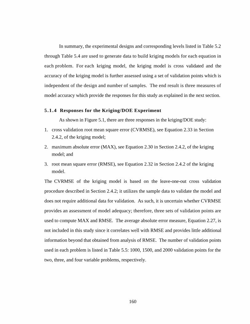
160
In summary, the experimental designs and corresponding levels listed in Table 5.2
through Table 5.4 are used to generate data to build kriging models for each equation in
each problem. For each kriging model, the kriging model is cross validated and the
accuracy of the kriging model is further assessed using a set of validation points which is
independent of the design and number of samples. The end result is three measures of
model accuracy which provide the responses for this study as explained in the next section.
5 .1 .4 Responses for the Kriging/DOE Experiment
As shown in Figure 5.1, there are three responses in the kriging/DOE study:
1. cross validation root mean square error (CVRMSE), see Equation 2.33 in Section
2.4.2, of the kriging model;
2. maximum absolute error (MAX), see Equation 2.30 in Section 2.4.2, of the kriging
model; and
3. root mean square error (RMSE), see Equation 2.32 in Section 2.4.2 of the kriging
model.
The CVRMSE of the kriging model is based on the leave-one-out cross validation
procedure described in Section 2.4.2; it utilizes the sample data to validate the model and
does not require additional data for validation. As such, it is uncertain whether CVRMSE
provides an assessment of model adequacy; therefore, three sets of validation points are
used to compute MAX and RMSE. The average absolute error measure, Equation 2.27, is
not included in this study since it correlates well with RMSE and provides little additional
information beyond that obtained from analysis of RMSE. The number of validation points
used in each problem is listed in Table 5.5: 1000, 1500, and 2000 validation points for the
two, three, and four variable problems, respectively.
161
Table 5.5 Additional Random Points Used to Assess Model Accuracy
Test Problem Name of Problem # Points2 variables Two-bar truss & Sym. three-bar truss 10003 variables Two-member frame & Helical spring 15004 variables Pressure vessel & Welded beam 2000
Rather than randomly pick these validation points, the points are obtained from a
random Latin hypercube to ensure uniformity within the design space. The predicted
values from each kriging model are compared against the actual values from the set of
validation points, and the error measures MAX and RMSE are computed. These measures
are then “normalized” as a percentage of the sample range, for the particular design under
investigation, in order to compare responses with different magnitudes. A precursory
analysis of the data is given in the next section.
5.2 PRECURSORY KRIGING/DOE DATA ANALYSIS AND ANOVA
In total, there are 11535 kriging models constructed as shown in Table 5.6 for the
six test problems—one kriging model for each equation for each design for each test
problem. For each of these models, there are three measures of model accuracy: MAX,
RMSE, and CVRMSE; hence, there are 34605 data points in the resulting data set.
Table 5.6 Kriging Test Problem Model Summary
ProblemName
No. ofVariables
No. ofResponses
No. ofUnique DOE
Total No.of DOE
No. ofCORFCN
No. ofModels
No. of TotalModels
2bar 2 3 51 71 5 765 10053bar 2 4 51 71 5 1020 1340
2mem 3 3 63 92 5 945 1380spring 3 7 63 92 5 2205 3220press 4 4 66 102 5 1320 2040weld 4 5 66 102 5 1650 2550
Grand Totals 7905 11535
162
To facilitate analysis of the data set, the error measures of the designs which are
replicated—the orthogonal arrays, random Latin hypercubes, OA-based Latin hypercubes,
and orthogonal Latin hypercubes—are averaged to reduce the data set to 7905 models.
However, not all of these 7905 models are good, i.e., many contain outliers which bias the
results, and potential outliers must be removed. The cause of the outliers can be attributed
to incomplete convergence of the numerical optimization used to fit the model or
singularities in the data set which occur during model fitting, numerical round-off error, or
bad data resulting from transferring data from file to file, program to program, and
computer to computer.
Hence, the data set is culled to remove any potential outliers. Rather than first fit
the model and remove potential outliers based on the residuals, the data is culled based on
(a) potential RMSE outliers, (b) potential MAX outliers, and (c) potential CVRMSE
outliers since it is known that many outliers exist due to singularities in the data set which
occur during model fitting. The process is described in detail in Appendix E; density plots
are included in Appendix E to show the distribution of the resulting data for the two, three,
and four variable problems.
In this manner, the data set is reduced from 7905 models to 7578. This constitutes
a reduction of about 4% which is considered reasonable given the magnitude of the study
and the potential for errors. From this point forward, any reference to “the data set” refers
to the final culled data set with all of the potential outliers removed and not to the original
data set unless explicitly specified.
Analysis of variance is performed in the next section to determine which factors
have a significant effect on the accuracy of the resulting kriging model. This is followed in
Section 5.2.2 with an examination of the correlation of the resulting error measures.
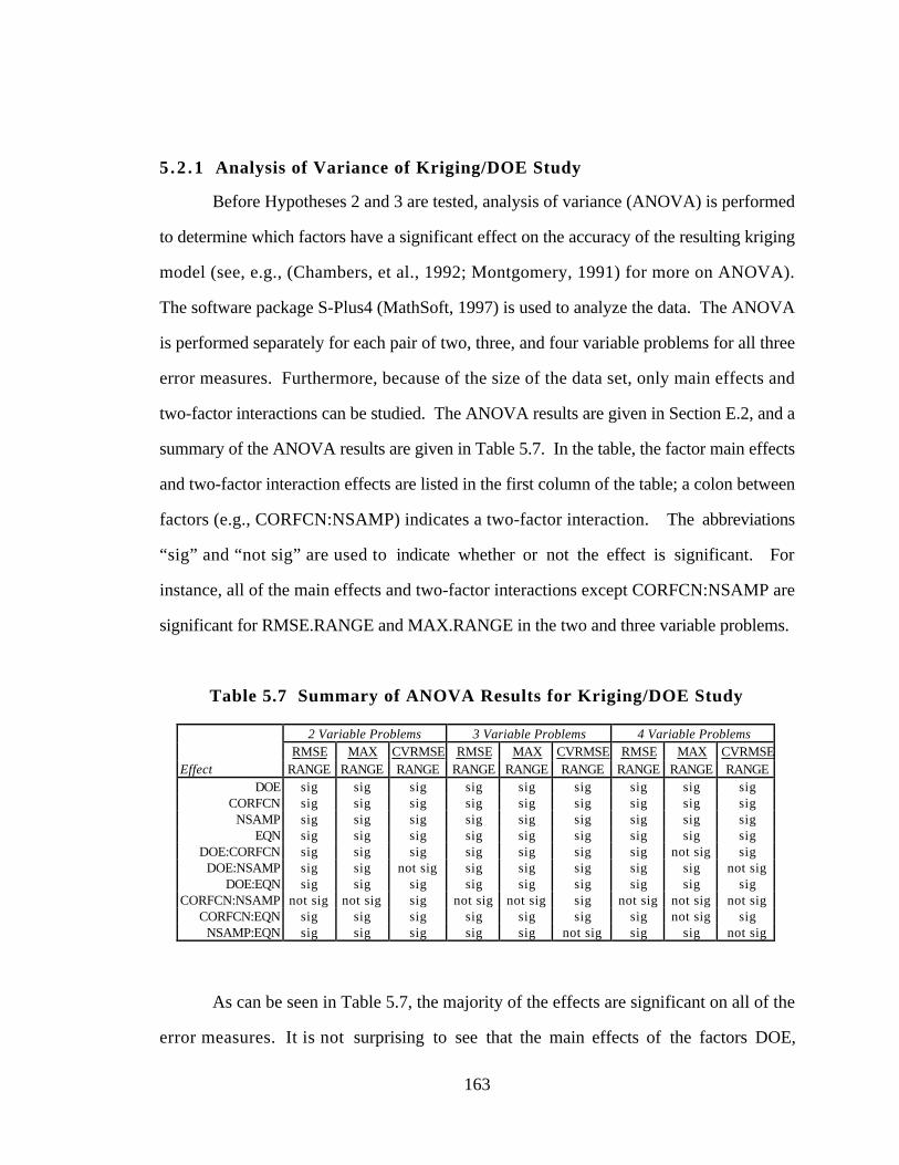
163
5 .2 .1 Analysis of Variance of Kriging/DOE Study
Before Hypotheses 2 and 3 are tested, analysis of variance (ANOVA) is performed
to determine which factors have a significant effect on the accuracy of the resulting kriging
model (see, e.g., (Chambers, et al., 1992; Montgomery, 1991) for more on ANOVA).
The software package S-Plus4 (MathSoft, 1997) is used to analyze the data. The ANOVA
is performed separately for each pair of two, three, and four variable problems for all three
error measures. Furthermore, because of the size of the data set, only main effects and
two-factor interactions can be studied. The ANOVA results are given in Section E.2, and a
summary of the ANOVA results are given in Table 5.7. In the table, the factor main effects
and two-factor interaction effects are listed in the first column of the table; a colon between
factors (e.g., CORFCN:NSAMP) indicates a two-factor interaction. The abbreviations
“sig” and “not sig” are used to indicate whether or not the effect is significant. For
instance, all of the main effects and two-factor interactions except CORFCN:NSAMP are
significant for RMSE.RANGE and MAX.RANGE in the two and three variable problems.
Table 5.7 Summary of ANOVA Results for Kriging/DOE Study
2 Variable Problems 3 Variable Problems 4 Variable Problems RMSE MAX CVRMSE RMSE MAX CVRMSE RMSE MAX CVRMSE
Effect RANGE RANGE RANGE RANGE RANGE RANGE RANGE RANGE RANGEDOE sig sig sig sig sig sig sig sig sig
CORFCN sig sig sig sig sig sig sig sig sigNSAMP sig sig sig sig sig sig sig sig sig
EQN sig sig sig sig sig sig sig sig sigDOE:CORFCN sig sig sig sig sig sig sig not sig sig
DOE:NSAMP sig sig not sig sig sig sig sig sig not sigDOE:EQN sig sig sig sig sig sig sig sig sig
CORFCN:NSAMP not sig not sig sig not sig not sig sig not sig not sig not sigCORFCN:EQN sig sig sig sig sig sig sig not sig sig
NSAMP:EQN sig sig sig sig sig not sig sig sig not sig
As can be seen in Table 5.7, the majority of the effects are significant on all of the
error measures. It is not surprising to see that the main effects of the factors DOE,
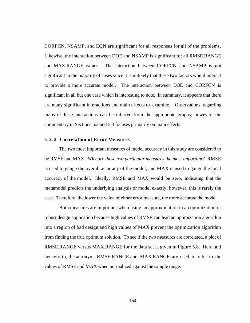
164
CORFCN, NSAMP, and EQN are significant for all responses for all of the problems.
Likewise, the interaction between DOE and NSAMP is significant for all RMSE.RANGE
and MAX.RANGE values. The interaction between CORFCN and NSAMP is not
significant in the majority of cases since it is unlikely that these two factors would interact
to provide a more accurate model. The interaction between DOE and CORFCN is
significant in all but one case which is interesting to note. In summary, it appears that there
are many significant interactions and main effects to examine. Observations regarding
many of these interactions can be inferred from the appropriate graphs; however, the
commentary in Sections 5.3 and 5.4 focuses primarily on main effects.
5 .2 .2 Correlation of Error Measures
The two most important measures of model accuracy in this study are considered to
be RMSE and MAX. Why are these two particular measures the most important? RMSE
is used to gauge the overall accuracy of the model, and MAX is used to gauge the local
accuracy of the model. Ideally, RMSE and MAX would be zero, indicating that the
metamodel predicts the underlying analysis or model exactly; however, this is rarely the
case. Therefore, the lower the value of either error measure, the more accurate the model.
Both measures are important when using an approximation in an optimization or
robust design application because high values of RMSE can lead an optimization algorithm
into a region of bad design and high values of MAX prevent the optimization algorithm
from finding the true optimum solution. To see if the two measures are correlated, a plot of
RMSE.RANGE versus MAX.RANGE for the data set is given in Figure 5.8. Here and
henceforth, the acronyms RMSE.RANGE and MAX.RANGE are used to refer to the
values of RMSE and MAX when normalized against the sample range.
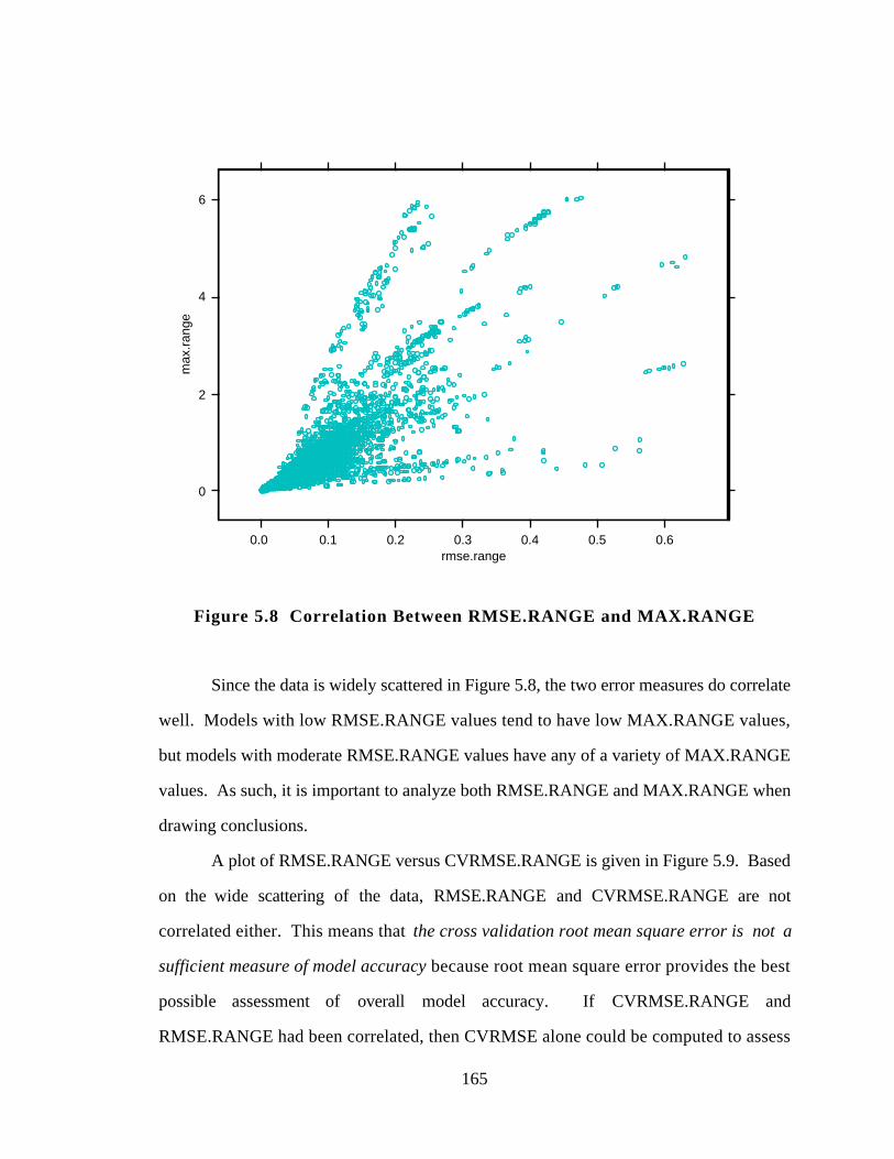
165
0.0 0.1 0.2 0.3 0.4 0.5 0.6rmse.range
0
2
4
6m
ax.r
ange
Figure 5.8 Correlation Between RMSE.RANGE and MAX.RANGE
Since the data is widely scattered in Figure 5.8, the two error measures do correlate
well. Models with low RMSE.RANGE values tend to have low MAX.RANGE values,
but models with moderate RMSE.RANGE values have any of a variety of MAX.RANGE
values. As such, it is important to analyze both RMSE.RANGE and MAX.RANGE when
drawing conclusions.
A plot of RMSE.RANGE versus CVRMSE.RANGE is given in Figure 5.9. Based
on the wide scattering of the data, RMSE.RANGE and CVRMSE.RANGE are not
correlated either. This means that the cross validation root mean square error is not a
sufficient measure of model accuracy because root mean square error provides the best
possible assessment of overall model accuracy. If CVRMSE.RANGE and
RMSE.RANGE had been correlated, then CVRMSE alone could be computed to assess
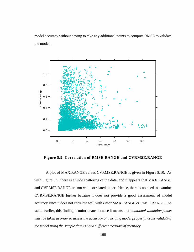
166
model accuracy without having to take any additional points to compute RMSE to validate
the model.
0.0 0.1 0.2 0.3 0.4 0.5 0.6rmse.range
0.0
0.2
0.4
0.6
0.8
1.0
cvrm
se.r
ange
Figure 5.9 Correlation of RMSE.RANGE and CVRMSE.RANGE
A plot of MAX.RANGE versus CVRMSE.RANGE is given in Figure 5.10. As
with Figure 5.9, there is a wide scattering of the data, and it appears that MAX.RANGE
and CVRMSE.RANGE are not well correlated either. Hence, there is no need to examine
CVRMSE.RANGE further because it does not provide a good assessment of model
accuracy since it does not correlate well with either MAX.RANGE or RMSE.RANGE. As
stated earlier, this finding is unfortunate because it means that additional validation points
must be taken in order to assess the accuracy of a kriging model properly; cross validating
the model using the sample data is not a sufficient measure of accuracy.
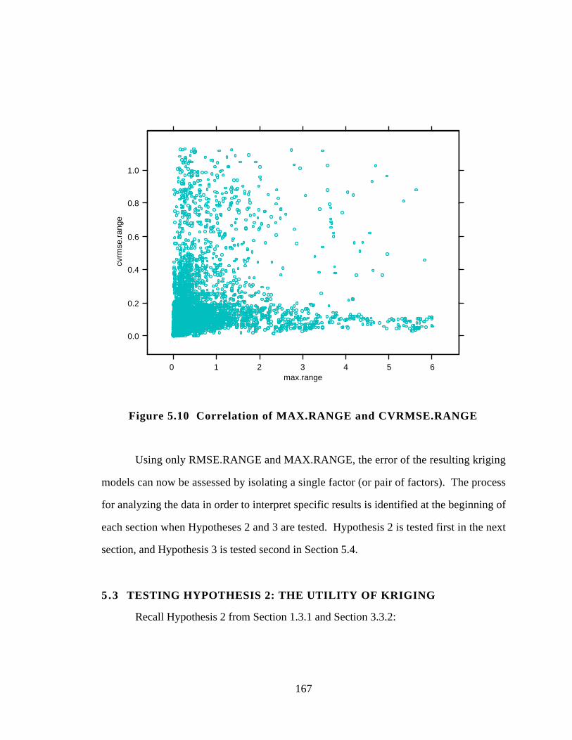
167
0 1 2 3 4 5 6max.range
0.0
0.2
0.4
0.6
0.8
1.0
cvrm
se.r
ange
Figure 5.10 Correlation of MAX.RANGE and CVRMSE.RANGE
Using only RMSE.RANGE and MAX.RANGE, the error of the resulting kriging
models can now be assessed by isolating a single factor (or pair of factors). The process
for analyzing the data in order to interpret specific results is identified at the beginning of
each section when Hypotheses 2 and 3 are tested. Hypothesis 2 is tested first in the next
section, and Hypothesis 3 is tested second in Section 5.4.
5.3 TESTING HYPOTHESIS 2: THE UTILITY OF KRIGING
Recall Hypothesis 2 from Section 1.3.1 and Section 3.3.2:
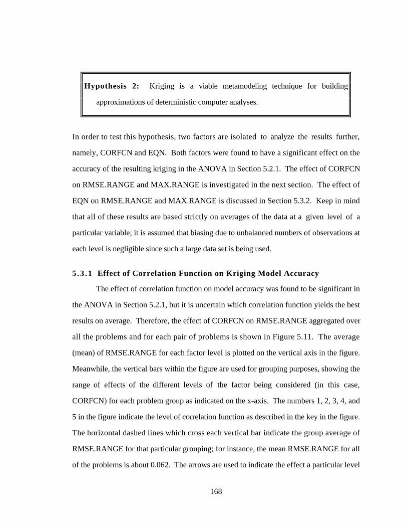
168
Hypothesis 2: Kriging is a viable metamodeling technique for building
approximations of deterministic computer analyses.
In order to test this hypothesis, two factors are isolated to analyze the results further,
namely, CORFCN and EQN. Both factors were found to have a significant effect on the
accuracy of the resulting kriging in the ANOVA in Section 5.2.1. The effect of CORFCN
on RMSE.RANGE and MAX.RANGE is investigated in the next section. The effect of
EQN on RMSE.RANGE and MAX.RANGE is discussed in Section 5.3.2. Keep in mind
that all of these results are based strictly on averages of the data at a given level of a
particular variable; it is assumed that biasing due to unbalanced numbers of observations at
each level is negligible since such a large data set is being used.
5 .3 .1 Effect of Correlation Function on Kriging Model Accuracy
The effect of correlation function on model accuracy was found to be significant in
the ANOVA in Section 5.2.1, but it is uncertain which correlation function yields the best
results on average. Therefore, the effect of CORFCN on RMSE.RANGE aggregated over
all the problems and for each pair of problems is shown in Figure 5.11. The average
(mean) of RMSE.RANGE for each factor level is plotted on the vertical axis in the figure.
Meanwhile, the vertical bars within the figure are used for grouping purposes, showing the
range of effects of the different levels of the factor being considered (in this case,
CORFCN) for each problem group as indicated on the x-axis. The numbers 1, 2, 3, 4, and
5 in the figure indicate the level of correlation function as described in the key in the figure.
The horizontal dashed lines which cross each vertical bar indicate the group average of
RMSE.RANGE for that particular grouping; for instance, the mean RMSE.RANGE for all
of the problems is about 0.062. The arrows are used to indicate the effect a particular level

169
of CORFCN has on RMSE.RANGE; the same holds true regardless of the factor being
considered. For example, in Figure 5.11 the average effect of CORFCN = 1 in the two
variable problems is slightly less than 0.08 while the average effect of CORFCN = 4 in the
same problems is slightly greater than 0.06. Finally, lower values of RMSE.RANGE (and
MAX.RANGE) are better; so, the lower the arrow of a particular level on the vertical line,
the more accurate is the resulting kriging model.
mea
n of
rm
se.r
ange
0.05
0.06
0.07
0.08
1
2
345
1
23
4
5
1
2
3
4
5
1
2
34
5
Factor - CORFCN
2 variable problems 3 variable problems 4 variable problemsall problems
Key:1 = Exponential2 = Gaussian3 = Cubic4 = Linear Matérn5 = Qaud. Matérn
Figure 5.11 Effect of Correlation Function Type on RMSE.RANGE
Some observations regarding Figure 5.11 are as follows. The exponential
correlation function (CORFCN = 1) repeatedly is the worst. Overall, the Gaussian
correlation function (CORFCN = 2) provides the lowest RMSE.RANGE on average and
also for the three and four variable problems as well. The linear Matérn (CORFCN = 4)
170
yields the lowest average RMSE.RANGE for the two variable problems but yields
comparable results to the piece-wise cubic correlation function (CORFCN = 3) and the
quadratic Matérn (CORFCN = 5) correlation function otherwise. The piece-wise cubic
(CORFCN = 3) and quadratic Matérn (CORFCN = 5) correlation functions generally yield
worse results than the Gaussian correlation function (CORFCN = 2).
The effect of CORFCN on MAX.RANGE is shown in Figure 5.12. As in Figure
5.11, the exponential correlation function (CORFCN = 1) repeatedly is the worst but does
surprisingly well in the four variable case. Overall, the Gaussian correlation function
(CORFCN = 2) provides the lowest MAX.RANGE on average and for the three and four
variable problems as well.
mea
n of
max
.ran
ge
0.4
0.5
0.6
0.7
1
2
34
5
1
23
4
5
1
2
345
12
345
Factor - CORFCN
2 variable problems 3 variable problems 4 variable problemsall problems
Key:1 = Exponential2 = Gaussian3 = Cubic4 = Linear Matérn5 = Qaud. Matérn
Figure 5.12 Effect of Correlation Function Type on MAX.RANGE
171
As seen in Figure 5.12, the linear Matérn correlation function (CORFCN = 4)
yields the best MAX.RANGE for the two variable problems and the worst for the four
variable problems with on average results otherwise. The piece-wise cubic (CORFCN = 3)
and quadratic Matérn (CORFCN = 5) correlation functions yield comparable results, falling
somewhere in the middle of the spectrum in each problem and performing slightly better
than average overall.
In summary, the Gaussian correlation function (CORFCN = 2) is the best
correlation function to use for building kriging models. On average, it provides the lowest
RMSE.RANGE and MAX.RANGE, yielding the most accurate kriging models.
Furthermore, it also yields the best results in the three and four variable problems when
averaged over all designs, sample sizes, and equations; in the two variable problems its
performance is average but not far behind the linear Matérn correlation function (CORFCN
= 4).
5 .3 .2 Effects of Equation Type on Kriging Model Accuracy
In order to determine which types of equations are fit best, the factor EQN is used
to isolate which equations are well fit by the kriging models, thus explicitly testing
Hypothesis 2. A plot of the resulting RMSE.RANGE of the two, three, and four variable
problems for each level of the factor EQN is shown in Figure 5.13; the effect of each level
of EQN on the mean of RMSE.RANGE is averaged over all DOE, NSAMP, and
CORFCN for each problem. For clarity, dashed lines are used to indicate the 5% and 10%
RMSE.RANGE values. If a 5% level of model accuracy is used as a cut-off point, then 14
out of the 26 equations in this study are accurately modeled by kriging. If that cut-off is
raised to 10%, then 20 out of the 26 equations are accurately modeled by kriging.
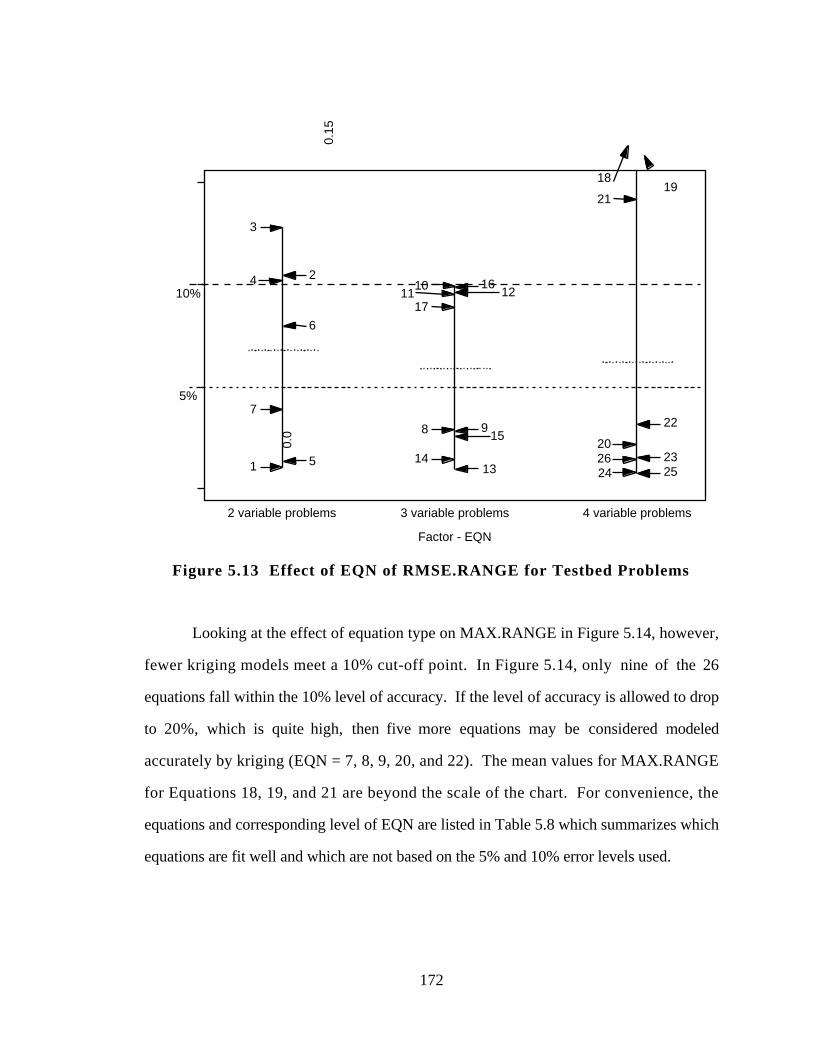
172
mea
n of
rm
se.r
ange
0.0
0.15
1
2
3
4
5
6
7
8 9
1011 12
1314
15
16
17
1819
20
21
22
2324 2526
Factor - EQN
2 variable problems 3 variable problems 4 variable problems
5%
10%
Figure 5.13 Effect of EQN of RMSE.RANGE for Testbed Problems
Looking at the effect of equation type on MAX.RANGE in Figure 5.14, however,
fewer kriging models meet a 10% cut-off point. In Figure 5.14, only nine of the 26
equations fall within the 10% level of accuracy. If the level of accuracy is allowed to drop
to 20%, which is quite high, then five more equations may be considered modeled
accurately by kriging (EQN = 7, 8, 9, 20, and 22). The mean values for MAX.RANGE
for Equations 18, 19, and 21 are beyond the scale of the chart. For convenience, the
equations and corresponding level of EQN are listed in Table 5.8 which summarizes which
equations are fit well and which are not based on the 5% and 10% error levels used.
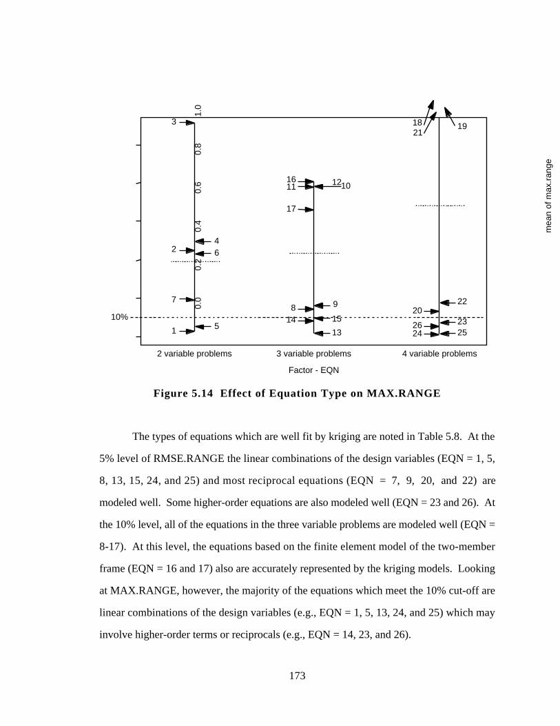
173
mea
n of
max
.ran
ge
0.0
0.2
0.4
0.6
0.8
1.0
1
2
3
4
5
6
7
Factor - EQN
8 9
1011 12
13
14 15
16
17
18 19
20
21
22
2324 2526
2 variable problems 3 variable problems 4 variable problems
10%
Figure 5.14 Effect of Equation Type on MAX.RANGE
The types of equations which are well fit by kriging are noted in Table 5.8. At the
5% level of RMSE.RANGE the linear combinations of the design variables (EQN = 1, 5,
8, 13, 15, 24, and 25) and most reciprocal equations (EQN = 7, 9, 20, and 22) are
modeled well. Some higher-order equations are also modeled well (EQN = 23 and 26). At
the 10% level, all of the equations in the three variable problems are modeled well (EQN =
8-17). At this level, the equations based on the finite element model of the two-member
frame (EQN = 16 and 17) also are accurately represented by the kriging models. Looking
at MAX.RANGE, however, the majority of the equations which meet the 10% cut-off are
linear combinations of the design variables (e.g., EQN = 1, 5, 13, 24, and 25) which may
involve higher-order terms or reciprocals (e.g., EQN = 14, 23, and 26).
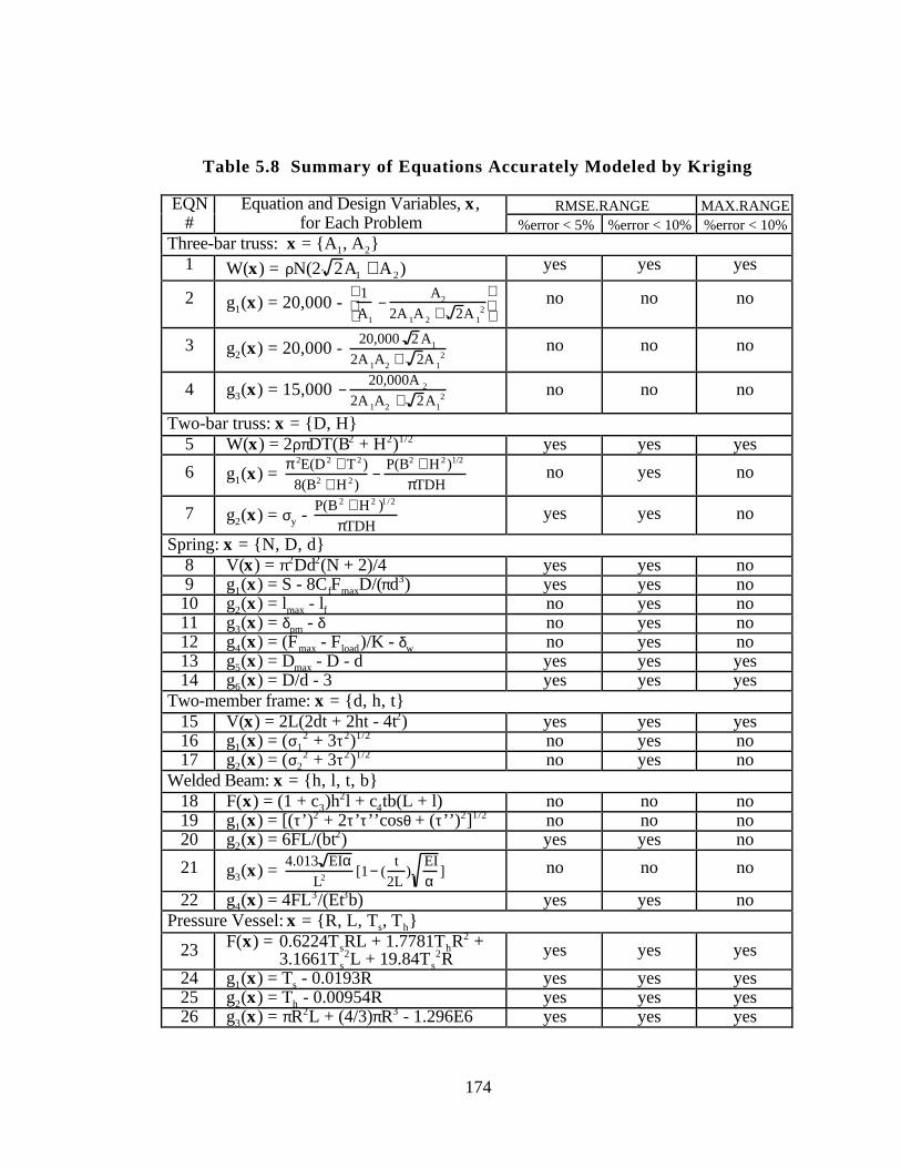
174
Table 5.8 Summary of Equations Accurately Modeled by Kriging
EQN Equation and Design Variables, x , RMSE.RANGE MAX.RANGE# for Each Problem %error < 5% %error < 10% %error < 10%
Three-bar truss: x = {A1, A2}1 W(x) = ρN(2 2A1 + A2) yes yes yes
2 g1(x) = 20,000 - 1
A1
−A2
2A 1A 2 + 2A 12
no no no
3 g2(x) = 20,000 - 20,000 2 A1
2A 1A2 + 2A 12
no no no
4 g3(x) = 15,000 −20,000A 2
2A 1A2 + 2A12 no no no
Two-bar truss: x = {D, H}5 W(x) = 2ρπDT(B2 + H2)1/2 yes yes yes
6 g1(x) = π 2E(D 2 + T 2 )
8(B2 + H 2 )−
P(B2 + H 2 )1/2
πTDHno yes no
7 g2(x) = σy - P(B 2 + H 2 )1/2
πTDHyes yes no
Spring: x = {N, D, d}8 V(x) = π2Dd2(N + 2)/4 yes yes no9 g1(x) = S - 8CfFmaxD/(πd3) yes yes no10 g2(x) = lmax - lf no yes no11 g3(x) = δpm - δ no yes no12 g4(x) = (Fmax - Fload)/K - δw no yes no13 g5(x) = Dmax - D - d yes yes yes14 g6(x) = D/d - 3 yes yes yes
Two-member frame: x = {d, h, t}15 V(x) = 2L(2dt + 2ht - 4t2) yes yes yes16 g1(x) = (σ1
2 + 3τ2)1/2 no yes no17 g2(x) = (σ2
2 + 3τ2)1/2 no yes noWelded Beam: x = {h, l, t, b}
18 F(x) = (1 + c3)h2l + c4tb(L + l) no no no
19 g1(x) = [(τ’)2 + 2τ’τ’’cosθ + (τ’’)2]1/2 no no no20 g2(x) = 6FL/(bt2) yes yes no
21 g3(x) = 4.013 EIα
L2 [1− (t
2L)
EI
α] no no no
22 g4(x) = 4FL3/(Et3b) yes yes noPressure Vessel: x = {R, L, Ts, Th}
23 F(x) = 0.6224TsRL + 1.7781ThR2 +
3.1661Ts2L + 19.84Ts
2R yes yes yes
24 g1(x) = Ts - 0.0193R yes yes yes25 g2(x) = Th - 0.00954R yes yes yes26 g3(x) = πR2L + (4/3)πR3 - 1.296E6 yes yes yes
175
Which types of functions are not modeled well by kriging? Based on the data in
Table 5.8, the equations which are not modeled well by kriging are the equations involving
reciprocals of combinations of the design variables in the three-bar truss problem (EQN =
2, 3, and 4) and two-bar truss problems (EQN = 6 and 7), and the majority of the welded
beam equations which include shear stress calculations, a cosine term which is a function
of the design variables, and a variety of reciprocals and square roots of terms which are
functions of the design variables. In addition, the finite element equations for the two-
member frame (EQN = 16 and 17) are not modeled well at the 5% level accuracy or at the
10% level of accuracy of MAX.RANGE. It is also interesting to note that the objective
function of the welded beam problem (EQN = 18) is one of the equations approximated
worst by the kriging. This is rather surprising considering it is very similar to the objective
function of the pressure vessel problem (EQN = 23) which is modeled well in all cases.
Perhaps these differences are due to the size of the design space as opposed to the
equations themselves; very few approximation methods will work well if the points are
sparsely scattered throughout the design space which may be the case in welded beam
problem and the three-bar truss problem.
In summary, it appears that kriging does provide an accurate approximation of a
variety of equations. Using a 5% level of accuracy, over half (14 out of the 26) of the
equations studied are accurately modeled over the entire design space as measured by
RMSE.RANGE; if a 10% level of accuracy is used instead, then over 3/4 of the equations
(20 out of 26) are accurately modeled. Unfortunately, only nine of the 26 meet the 10%
level of accuracy in MAX.RANGE; however, of the two measures, RMSE.RANGE is
considered to be more important from a design standpoint since accuracy over the entire
design space is more important during design space search than the maximum discrepancy
at any one given point. As such, Hypothesis 2 is verified. In the next section, Hypothesis
3 is tested.
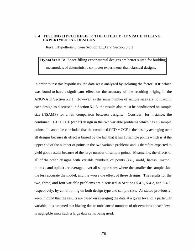
176
5.4 TESTING HYPOTHESIS 3: THE UTILITY OF SPACE FILLINGEXPERIMENTAL DESIGNS
Recall Hypothesis 3 from Section 1.1.3 and Section 3.3.2.
Hypothesis 3: Space filling experimental designs are better suited for building
metamodels of deterministic computer experiments than classical designs.
In order to test this hypothesis, the data set is analyzed by isolating the factor DOE which
was found to have a significant effect on the accuracy of the resulting kriging in the
ANOVA in Section 5.2.1. However, as the same number of sample sizes are not used in
each design as discussed in Section 5.1.3, the results also must be conditioned on sample
size (NSAMP) for a fair comparison between designs. Consider, for instance, the
combined CCD + CCF (ccdaf) design in the two variable problems which has 13 sample
points. It cannot be concluded that the combined CCD + CCF is the best by averaging over
all designs because its effect is biased by the fact that it has 13 sample points which is at the
upper end of the number of points in the two variable problems and is therefore expected to
yield good results because of the large number of sample points. Meanwhile, the effects of
all of the other designs with variable numbers of points (i.e., unifd, hamss, mxmnl,
mnmxl, and oplhd) are averaged over all sample sizes where the smaller the sample size,
the less accurate the model, and the worse the effect of these designs. The results for the
two, three, and four variable problems are discussed in Sections 5.4.1, 5.4.2, and 5.4.3,
respectively, by conditioning on both design type and sample size. As stated previously,
keep in mind that the results are based on averaging the data at a given level of a particular
variable; it is assumed that biasing due to unbalanced numbers of observations at each level
is negligible since such a large data set is being used.

177
5 .4 .1 Comparison of Designs for Two Variable Problems
For the two variable problems, the classical designs (CCI, CCF, and CCD) each
utilize nine sample points, and the combined CCF + CCI and CCF + CCD each have 13
points. Hence, the average effect of each design which has nine points and each design
which has 13 points on RMSE.RANGE is shown in Figure 5.15. The average effect on
MAX.RANGE of all the designs with these sample sizes is shown in Figure 5.16.
Looking first at the nine point designs in Figure 5.15, it is surprising to note that
both the CCD and CCI designs perform well with the minimax Latin hypercube (mnmxl)
design yielding the best RMSE.RANGE values; recall that the minimax Latin hypercube
designs are unique to this research (see Appendix C). The orthogonal Latin hypercubes
(yelhd), maximin Latin hypercubes (mxmnl), and the uniform designs (unifd) also perform
well. The worst designs are the Hammersley sampling sequence design, the CCF design
and the OA-based Latin hypercube. The random Latin hypercubes yield average results.
In the 13 point designs, the uniform design (unifd) yields the best results with the
maximin and minimax Latin hypercube designs giving equally good results which are only
slightly worse than that of the uniform design. The random Latin hypercubes (rnlhd)
continue to give average results with the combined CCD + CCF (ccdaf) and CCI + CCF
(cciaf) designs giving slightly better results but results which are still about 1% worse than
the maximin and minimax Latin hypercubes. The optimal Latin hypercube designs are the
worst with the Hammersley sampling sequence designs showing good improvement with
the extra four sample points.
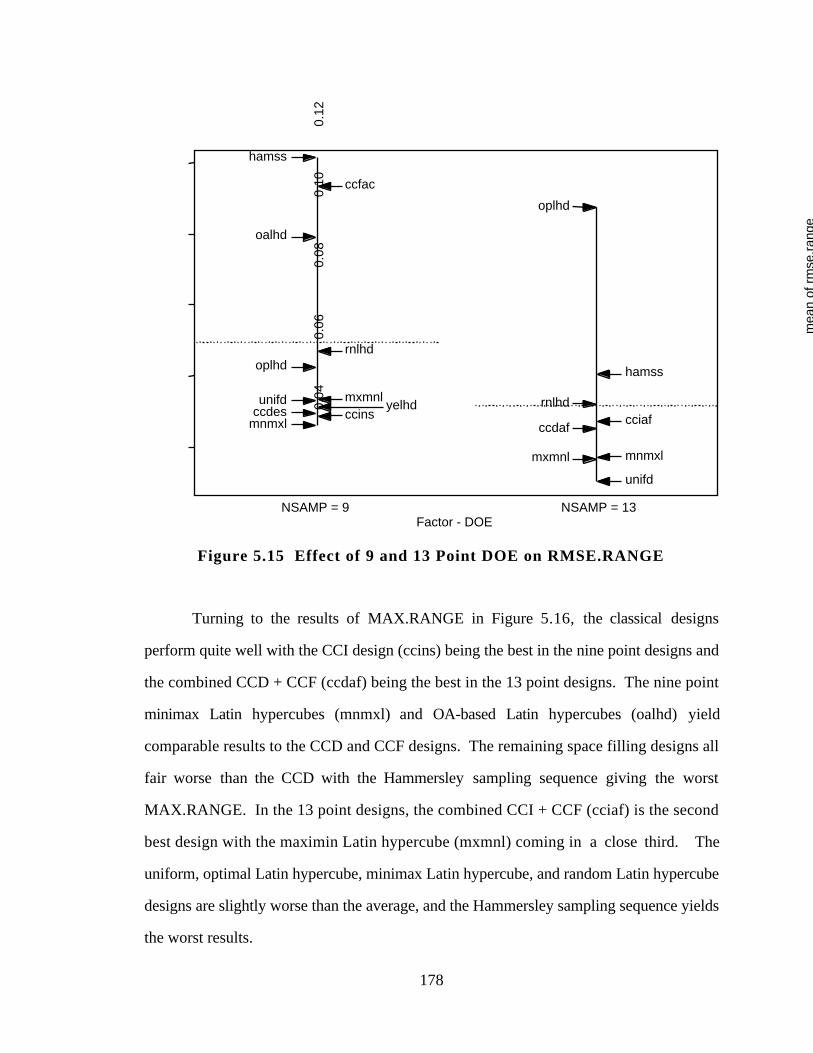
178
mea
n of
rm
se.r
ange
0.04
0.06
0.08
0.10
0.12
ccdes
ccfac
ccins
hamss
mnmxl
mxmnl
oalhd
oplhdrnlhd
unifd yelhd
Factor - DOE
ccdafcciaf
hamss
mnmxlmxmnl
oplhd
rnlhd
unifd
NSAMP = 9 NSAMP = 13
Figure 5.15 Effect of 9 and 13 Point DOE on RMSE.RANGE
Turning to the results of MAX.RANGE in Figure 5.16, the classical designs
perform quite well with the CCI design (ccins) being the best in the nine point designs and
the combined CCD + CCF (ccdaf) being the best in the 13 point designs. The nine point
minimax Latin hypercubes (mnmxl) and OA-based Latin hypercubes (oalhd) yield
comparable results to the CCD and CCF designs. The remaining space filling designs all
fair worse than the CCD with the Hammersley sampling sequence giving the worst
MAX.RANGE. In the 13 point designs, the combined CCI + CCF (cciaf) is the second
best design with the maximin Latin hypercube (mxmnl) coming in a close third. The
uniform, optimal Latin hypercube, minimax Latin hypercube, and random Latin hypercube
designs are slightly worse than the average, and the Hammersley sampling sequence yields
the worst results.
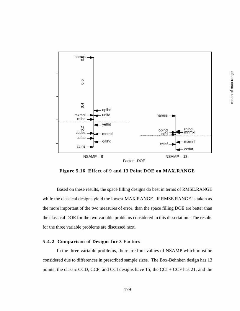
179
mea
n of
max
.ran
ge
0.2
0.4
0.6
0.8
ccdesccfac
ccins
hamss
mnmxl
mxmnl
oalhd
oplhd
rnlhdunifd
yelhd
ccdafcciaf
hamss
mnmxl
mxmnl
oplhd rnlhdunifd
Factor - DOENSAMP = 9 NSAMP = 13
Figure 5.16 Effect of 9 and 13 Point DOE on MAX.RANGE
Based on these results, the space filling designs do best in terms of RMSE.RANGE
while the classical designs yield the lowest MAX.RANGE. If RMSE.RANGE is taken as
the more important of the two measures of error, than the space filling DOE are better than
the classical DOE for the two variable problems considered in this dissertation. The results
for the three variable problems are discussed next.
5 .4 .2 Comparison of Designs for 3 Factors
In the three variable problems, there are four values of NSAMP which must be
considered due to differences in prescribed sample sizes. The Box-Behnken design has 13
points; the classic CCD, CCF, and CCI designs have 15; the CCI + CCF has 21; and the
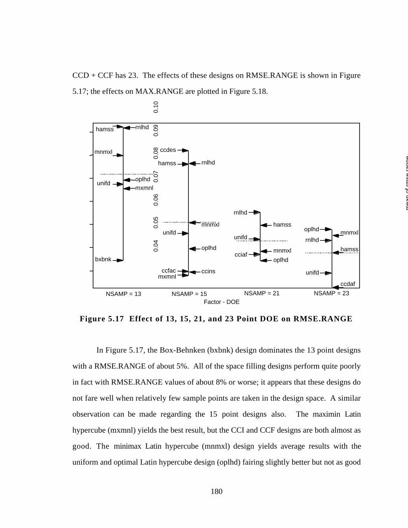
180
CCD + CCF has 23. The effects of these designs on RMSE.RANGE is shown in Figure
5.17; the effects on MAX.RANGE are plotted in Figure 5.18.
mea
n of
rm
se.r
ange
0.04
0.05
0.06
0.07
0.08
0.09
0.10
bxbnk
hamss
mnmxl
mxmnloplhd
rnlhd
unifd
Factor - DOENSAMP = 13
ccdes
ccfac ccins
hamss
mnmxl
mxmnl
oplhd
rnlhd
unifd
NSAMP = 15 NSAMP = 21 NSAMP = 23
cciaf
hamss
mnmxl
oplhd
rnlhd
unifd
ccdaf
hamss
mnmxloplhd
rnlhd
unifd
Figure 5.17 Effect of 13, 15, 21, and 23 Point DOE on RMSE.RANGE
In Figure 5.17, the Box-Behnken (bxbnk) design dominates the 13 point designs
with a RMSE.RANGE of about 5%. All of the space filling designs perform quite poorly
in fact with RMSE.RANGE values of about 8% or worse; it appears that these designs do
not fare well when relatively few sample points are taken in the design space. A similar
observation can be made regarding the 15 point designs also. The maximin Latin
hypercube (mxmnl) yields the best result, but the CCI and CCF designs are both almost as
good. The minimax Latin hypercube (mnmxl) design yields average results with the
uniform and optimal Latin hypercube design (oplhd) fairing slightly better but not as good

181
as the CCI and CCF. The CCD is the worse design with the random Latin hypercube
(rnlhd) and the Hammersley sampling sequence (hamss) yielding comparably poor results.
In the 21 and 23 point designs in Figure 5.17, the optimal Latin hypercube design
(oplhd) yields the lowest RMSE.RANGE with the random Latin hypercube design (rnlhd)
yielding the worst. The combined CCI + CCF (cciaf) is the second best 21 point design,
followed closely by the minimax Latin hypercube (mnmxl). The uniform design (unifd)
gives an average result in the 21 point case but is the second best design in the 23 point
case; the best design is the combined CCD + CCF (ccdaf). The optimal Latin hypercube
design (oplhd) is the worst of the 23 point designs with the minimax Latin hypercube
(mnmxl) and random Latin hypercube designs (rnlhd) yielding results which are worse
than the average.
In Figure 5.18, the effects of these different designs on MAX.RANGE are plotted.
The classical experimental designs consistently provided the lowest MAX.RANGE when
averaging over all other factors. The space filling designs do not perform well in any case
and yield particularly poor results in the 13 and 21 point designs. The minimax Latin
hypercube (mnmxl) design is no exception, giving near average results in 15, 21, and 23
point designs and the next to worst result among the 13 point designs.
As with the two variable problems, the space filling designs offer better results if
RMSE.RANGE is considered while the classical designs are better when it comes to
MAX.RANGE for the problems considered in this dissertation. The four variable
problems are examined in the next section to see if the same holds true.
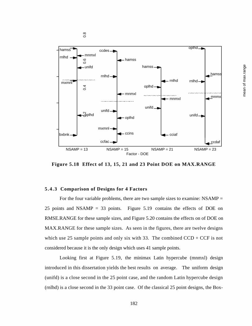
182
mea
n of
max
.ran
ge
0.2
0.4
0.6
0.8
bxbnk
hamssmnmxl
mxmnl
oplhd
rnlhd
unifd
ccdes
ccfac
ccins
hamss
mnmxl
mxmnl
oplhd
rnlhd
unifd
Factor - DOENSAMP = 13 NSAMP = 15 NSAMP = 21 NSAMP = 23
ccdaf
oplhd
rnlhd
unifd
hamss
mnmxl
cciaf
hamss
mnmxl
oplhd
rnlhd
unifd
Figure 5.18 Effect of 13, 15, 21 and 23 Point DOE on MAX.RANGE
5.4 .3 Comparison of Designs for 4 Factors
For the four variable problems, there are two sample sizes to examine: NSAMP =
25 points and NSAMP = 33 points. Figure 5.19 contains the effects of DOE on
RMSE.RANGE for these sample sizes, and Figure 5.20 contains the effects on of DOE on
MAX.RANGE for these sample sizes. As seen in the figures, there are twelve designs
which use 25 sample points and only six with 33. The combined CCD + CCF is not
considered because it is the only design which uses 41 sample points.
Looking first at Figure 5.19, the minimax Latin hypercube (mnmxl) design
introduced in this dissertation yields the best results on average. The uniform design
(unifd) is a close second in the 25 point case, and the random Latin hypercube design
(rnlhd) is a close second in the 33 point case. Of the classical 25 point designs, the Box-
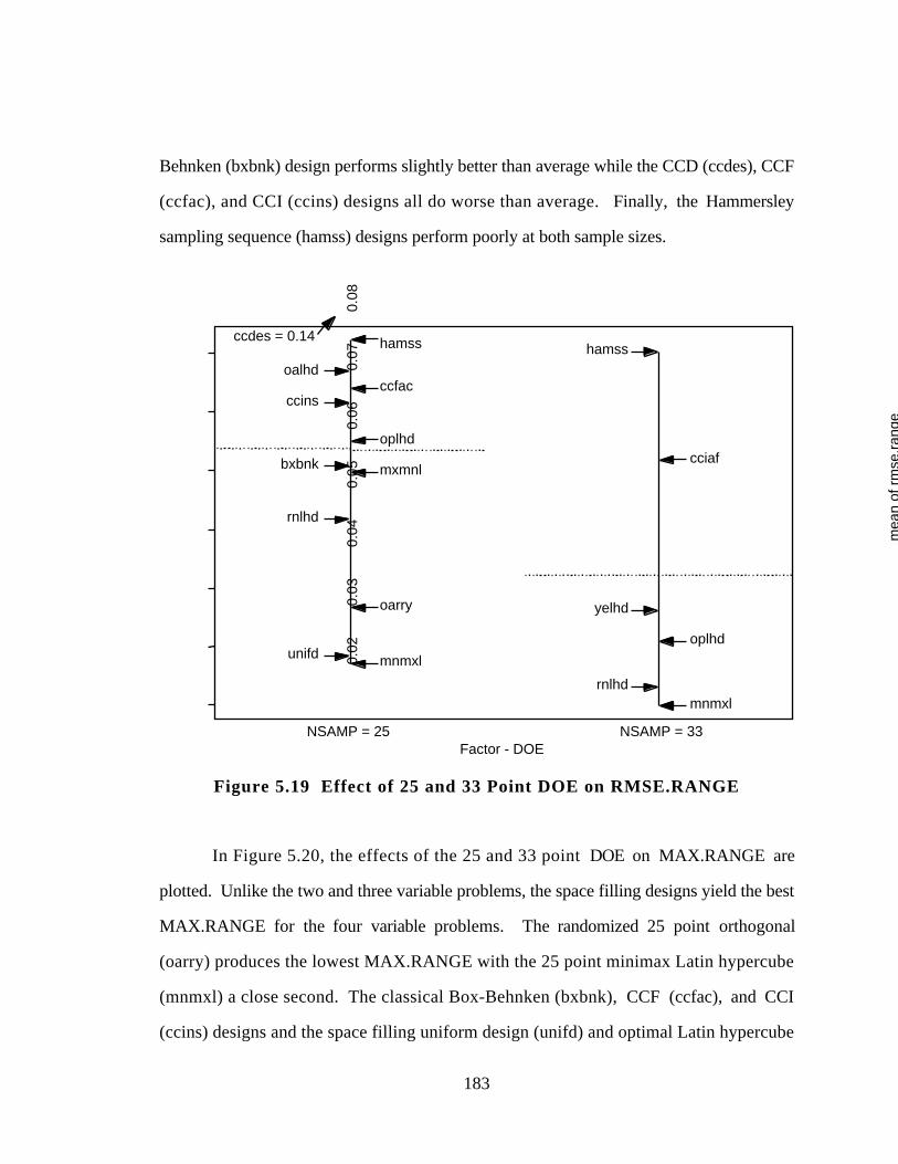
183
Behnken (bxbnk) design performs slightly better than average while the CCD (ccdes), CCF
(ccfac), and CCI (ccins) designs all do worse than average. Finally, the Hammersley
sampling sequence (hamss) designs perform poorly at both sample sizes.
mea
n of
rm
se.r
ange
0.02
0.03
0.04
0.05
0.06
0.07
0.08
bxbnk
ccdes = 0.14
ccfacccins
hamss
mnmxl
mxmnl
oalhd
oarry
oplhd
rnlhd
unifd
cciaf
hamss
mnmxl
oplhd
rnlhd
yelhd
Factor - DOENSAMP = 25 NSAMP = 33
Figure 5.19 Effect of 25 and 33 Point DOE on RMSE.RANGE
In Figure 5.20, the effects of the 25 and 33 point DOE on MAX.RANGE are
plotted. Unlike the two and three variable problems, the space filling designs yield the best
MAX.RANGE for the four variable problems. The randomized 25 point orthogonal
(oarry) produces the lowest MAX.RANGE with the 25 point minimax Latin hypercube
(mnmxl) a close second. The classical Box-Behnken (bxbnk), CCF (ccfac), and CCI
(ccins) designs and the space filling uniform design (unifd) and optimal Latin hypercube
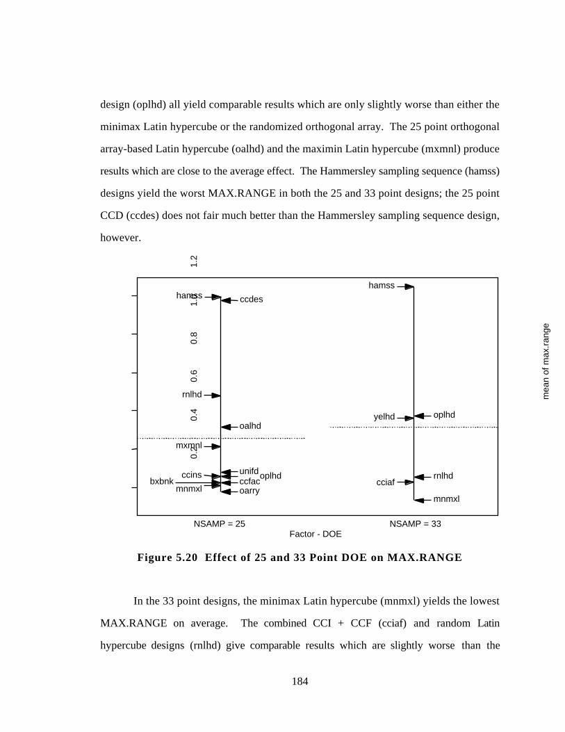
184
design (oplhd) all yield comparable results which are only slightly worse than either the
minimax Latin hypercube or the randomized orthogonal array. The 25 point orthogonal
array-based Latin hypercube (oalhd) and the maximin Latin hypercube (mxmnl) produce
results which are close to the average effect. The Hammersley sampling sequence (hamss)
designs yield the worst MAX.RANGE in both the 25 and 33 point designs; the 25 point
CCD (ccdes) does not fair much better than the Hammersley sampling sequence design,
however.
mea
n of
max
.ran
ge
0.2
0.4
0.6
0.8
1.0
1.2
bxbnk
ccdes
ccfacccins
hamss
mnmxl
mxmnl
oalhd
oarry
oplhd
rnlhd
unifdcciaf
hamss
mnmxl
oplhd
rnlhd
yelhd
Factor - DOENSAMP = 25 NSAMP = 33
Figure 5.20 Effect of 25 and 33 Point DOE on MAX.RANGE
In the 33 point designs, the minimax Latin hypercube (mnmxl) yields the lowest
MAX.RANGE on average. The combined CCI + CCF (cciaf) and random Latin
hypercube designs (rnlhd) give comparable results which are slightly worse than the
185
minimax Latin hypercube. Finally, the 33 point orthogonal Latin hypercubes (yelhd) and
optimal Latin hypercubes (oplhd) are both slightly worse than the average.
5 .4 .4 Lessons Learned from Experimental Design Study
The space filling designs yield lower RMSE.RANGE values for all of the two,
three, and four variable problems considered in this dissertation. The classical
experimental designs yield lower MAX.RANGE values for the two and three variable
problems but do not perform as well as the space filling designs in the four variable
problems. In small dimensions, i.e., two and three variables, the classical designs spread
the points out equally well in the design space regardless if they are “space filling” designs
or not. However, based on the observed trends in the data, it appears that as the number of
design variables increases, the space filling designs perform better and better in terms of the
two error measurements used in this study. As their name implies, the space filling designs
do a better job at spreading out points in the design space and thus filling the space as the
number of variables increases. Hence, Hypothesis 3 is verified because the space filling
designs do perform better than the classical designs in terms of RMSE.RANGE which
provides the best assessment of overall accuracy of a metamodel. Furthermore, the larger
the number of design variables and the more sample points, the better is the accuracy of the
resulting kriging model from a space filling design.
Some additional comments about particular space filling designs are as follows.
• The minimax Latin hypercube designs introduced in this dissertation perform quite
well in these problems. With the exception of the 13 point minimax Latin
hypercube design for the three variable problems, these designs consistently are
among the best of the designs in terms of its effect on RMSE.RANGE and
MAX.RANGE.
• The Hammersley sampling sequence designs perform poorly in all of these
problems. The impetus for the Hammersley designs, though, are to provide good
stratification of a k-dimensional space (Kalagnanam and Diwekar, 1997); as such,
186
they are designed to perform well in large design space which may explain why
they perform so poorly in these relatively small problems.
• The random Latin hypercube designs provide average results as might be expected
because these designs simply rely on a random scattering of points in the design
space. By imposing additional considerations on these designs to “control” the
randomization of the points, the performance of these designs can be improved.
For instance, the orthogonal Latin hypercubes (Ye, 1997), the maximin Latin
hypercubes (Morris and Mitchell, 1995), the (IMSE) optimal Latin hypercubes
(Park, 1994), and the orthogonal-array based Latin hypercubes (Tang, 1993)
typically yield a more accurate kriging model than does the basic random Latin
hypercube. This observation is not new; rather, it supports the claims which the
creators of these designs when they introduced them.
• The uniform designs perform surprisingly well, considering they are based solely
on number-theoretic reasoning (Fang and Wang, 1994). Regardless, the
importance of these designs lies in that fact that uniformly spreading the points out
the design space yields an accurate kriging model; this is a new observation which
is obvious but not well documented in the literature.
Hypotheses 2 and 3 have now been verified as a result of this study. In the next
section, the relevance of these results with regard to the PPCEM are discussed.
5.5 A LOOK BACK AND A LOOK AHEAD
In this chapter, 7905 kriging metamodels of six engineering test problems have
been constructed and validated using a variety of correlation functions and experimental
designs to test and verify Hypotheses 2 and 3. In closing this chapter, recall the questions
posed at the beginning of this study:
• What is best type of experimental design you should use to query the simulation to
generate data to build an accurate kriging metamodel? For problems containing
only two variables, either classical or space filling designs yield good results;
however, as the size of the design space increases (i.e., number of variables
increases), space filling experimental design tend to yield more accurate kriging
187
metamodels on average since they tend to spread the points out well in the design
space. In particular, the minimax Latin hypercube design, uniform designs, and
orthogonal arrays yield good results. Random Latin hypercubes also provide good
results, provided orthogonality or optimality (e.g., IMSE) are imposed to control
the randomization. Finally, of the designs considered, Hammersley point designs
are not recommended unless numerous sample points can be afforded.
• How many sample points should you use? The interaction between sample size and
experimental design type is examined in Section E.3 because this impact does not
directly impact testing Hypotheses 2 or 3 since the analysis is conditioned on
sample size. In general, the more sample points which can be afforded, the more
accurate the resulting model. However, as discussed in Section E.3, a
recommendation on the number of sample points cannot be made at this time
because a wide enough spread of points was not investigated.
• What type of correlation function should you use to obtain the best predictor?
Based on the results in Section 5.3.1, the Gaussian correlation function yields the
most accurate predictor on average of the five studied.
• Lastly, how can you best validate the metamodel once you have constructed it? As
discussed in Section 5.2.2, cross validation root mean square error is not a
sufficient measure of model accuracy since it does not correlate well with either root
mean square error or max. error. One possible explanation of this is that because
the sample sizes are relatively small, an insufficient number of points is available to
cross-validate the model properly. If more points were available, then cross
validation error may yield a reasonable assessment of model accuracy; however,
this has not been tested. In light of this result, then, it is imperative that additional
sample points be taken to validate a kriging model.
These results have a direct bearing on the metamodeling capabilities within the Product
Platform Concept Exploration Method (PPCEM) as depicted in Figure 5.21. In the event
that metamodels need to be constructed for a deterministic computer code or simulation
routine within the context of product platform design, then the best correlation function to
select—if kriging metamodels are to be utilized—is the Gaussian correlation function, and
the best design to use is a space filling experimental design if the problem has more than
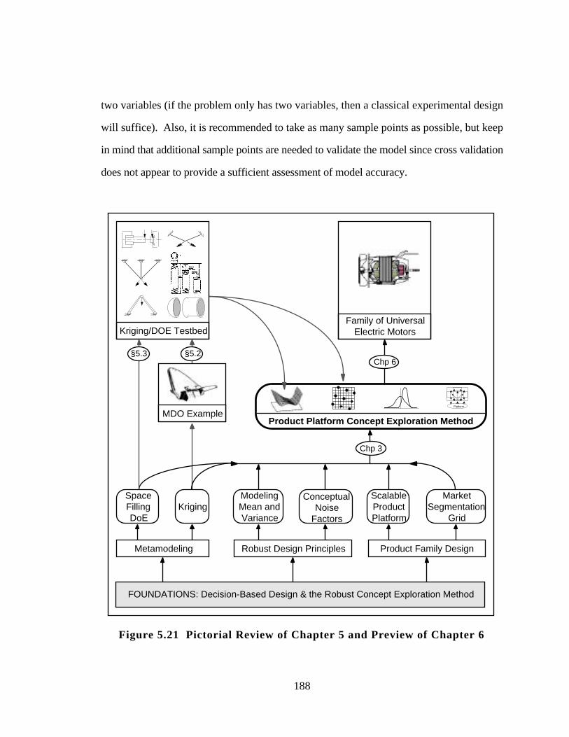
188
two variables (if the problem only has two variables, then a classical experimental design
will suffice). Also, it is recommended to take as many sample points as possible, but keep
in mind that additional sample points are needed to validate the model since cross validation
does not appear to provide a sufficient assessment of model accuracy.
Family of UniversalElectric Motors
Chp 6
Metamodeling
ModelingMean andVariance
Robust Design Principles
ConceptualNoise
Factors
ScalableProductPlatform
MarketSegmentation
Grid
Product Family Design
Chp 3
FOUNDATIONS: Decision-Based Design & the Robust Concept Exploration Method
Platform
Product Platform Concept Exploration Method
§5.3 §5.2
MDO Example
KrigingSpaceFillingDoE
Kriging/DOE Testbed
Figure 5.21 Pictorial Review of Chapter 5 and Preview of Chapter 6

189
In the next chapter, the focus returns to the PPCEM, and the process of testing and
verifying Hypotheses 1 resumes. Specifically, in Chapter 6 the design of a family of
universal electric motors is offered as “proof of concept” that the PPCEM works and that it
is effective at facilitating the design and development of a scalable product platform for a
product family.

190
6. CHAPTER 6
DESIGN OF A FAMILY OF UNIVERSALELECTRIC MOTORS
In this chapter, the Product Platform Concept Exploration Method (PPCEM) is
implemented to verify its use for designing a family of universal motors around a common
scalable product platform. An overview of the universal motor problem is presented in
Section 6.1; a schematic of a typical universal motor is given in Section 6.1.1, and a
practical mathematical model for universal motors is derived in Section 6.1.2. Section 6.2
contains the implementation of Steps 1 and 2 of the PPCEM. A market segmentation grid
is created for the problem and relevant factors and responses for the universal motor
platform are identified. Section 6.3 follows with the implementation of Step 4 of the
PPCEM by aggregating the universal motor specifications and formulating a compromise
DSP; Step 3 of the PPCEM—building metamodels—is not utilized in this example because
analytical expressions for mean and standard deviation of the responses are derived
separately. Section 6.4 contains the development of the actual universal motor platform;
ramifications of the resulting universal motor platform and product family are analyzed in
Section 6.5. Through this example problem, Hypothesis 1 and Sub-Hypotheses 1.1-1.3
are tested and verified as follows:
191
Hypothesis 1 - All but Step 3 of the PPCEM is employed in this chapter to design a
family of universal motors based on a scalable product platform. The success of
the method as discussed in Section 6.5 provides an initial “proof of concept” for the
method and hence Hypothesis 1.
Sub-Hypothesis 1.1 - The market segmentation grid is utilized in Section 6.2 to
help identify the stack length as the scale factor around which the motor family is
vertically scaled to achieve the desired platform leveraging strategy; this supports
Sub-Hypothesis 1.1.
Sub-Hypothesis 1.2 - The scale factor for the family of universal motors is taken as
the stack length, following the footsteps of the example by Black & Decker
(Lehnerd, 1987). Robust design principles are used in this example to develop a
universal motor platform—defined by seven design variables—which is insensitive
to variations in the scale factor and is thus good for a family of motors based on
different instantiations of the stack length (the scale factor). The success of this
implementation helps to support Sub-Hypothesis 1.2.
Sub-Hypothesis 1.3 - Robust design principles of “bringing the mean on target”
and “minimizing the deviation” are utilized in this example to aggregate individual
targets and constraints and to facilitate the design of the family of motors.
Combining this formulation with the compromise DSP allows a family of motors to
be designed around a common, scalable product platform, verifying Sub-
Hypothesis 1.3.
Despite all of the work in the previous two chapters, Hypotheses 2 and 3 are not
tested in this example. Analytic expressions for mean and standard deviation of the
response are derived from the analysis equations themselves and used directly in the
compromise DSP for the PPCEM. In concluding the chapter, a brief look ahead to the
General Aviation aircraft example in Chapter 7 in which the PPCEM is tested in full is
offered in Section 6.6.
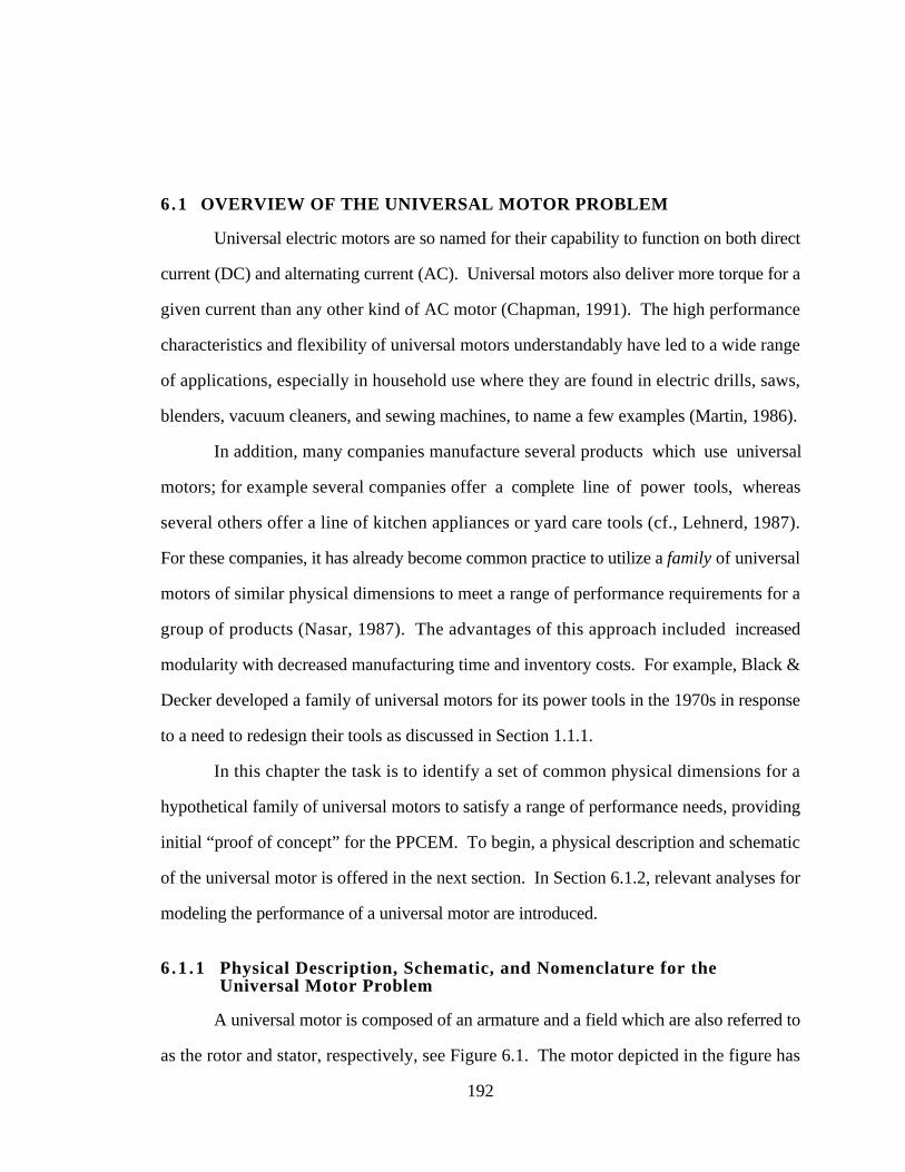
192
6.1 OVERVIEW OF THE UNIVERSAL MOTOR PROBLEM
Universal electric motors are so named for their capability to function on both direct
current (DC) and alternating current (AC). Universal motors also deliver more torque for a
given current than any other kind of AC motor (Chapman, 1991). The high performance
characteristics and flexibility of universal motors understandably have led to a wide range
of applications, especially in household use where they are found in electric drills, saws,
blenders, vacuum cleaners, and sewing machines, to name a few examples (Martin, 1986).
In addition, many companies manufacture several products which use universal
motors; for example several companies offer a complete line of power tools, whereas
several others offer a line of kitchen appliances or yard care tools (cf., Lehnerd, 1987).
For these companies, it has already become common practice to utilize a family of universal
motors of similar physical dimensions to meet a range of performance requirements for a
group of products (Nasar, 1987). The advantages of this approach included increased
modularity with decreased manufacturing time and inventory costs. For example, Black &
Decker developed a family of universal motors for its power tools in the 1970s in response
to a need to redesign their tools as discussed in Section 1.1.1.
In this chapter the task is to identify a set of common physical dimensions for a
hypothetical family of universal motors to satisfy a range of performance needs, providing
initial “proof of concept” for the PPCEM. To begin, a physical description and schematic
of the universal motor is offered in the next section. In Section 6.1.2, relevant analyses for
modeling the performance of a universal motor are introduced.
6 .1 .1 Physical Description, Schematic, and Nomenclature for theUniversal Motor Problem
A universal motor is composed of an armature and a field which are also referred to
as the rotor and stator, respectively, see Figure 6.1. The motor depicted in the figure has
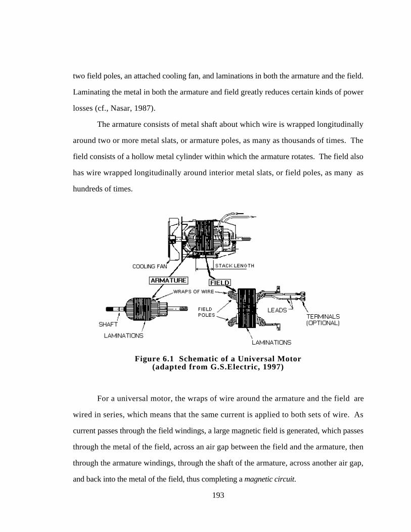
193
two field poles, an attached cooling fan, and laminations in both the armature and the field.
Laminating the metal in both the armature and field greatly reduces certain kinds of power
losses (cf., Nasar, 1987).
The armature consists of metal shaft about which wire is wrapped longitudinally
around two or more metal slats, or armature poles, as many as thousands of times. The
field consists of a hollow metal cylinder within which the armature rotates. The field also
has wire wrapped longitudinally around interior metal slats, or field poles, as many as
hundreds of times.
Figure 6.1 Schematic of a Universal Motor(adapted from G.S.Electric, 1997)
For a universal motor, the wraps of wire around the armature and the field are
wired in series, which means that the same current is applied to both sets of wire. As
current passes through the field windings, a large magnetic field is generated, which passes
through the metal of the field, across an air gap between the field and the armature, then
through the armature windings, through the shaft of the armature, across another air gap,
and back into the metal of the field, thus completing a magnetic circuit.

194
However when the magnetic field passes though the armature windings, which are
themselves carrying current, the magnetic field exerts a force on the current carrying wires,
which is in the direction of the cross product of the vector direction of the current in the
armature windings and the vector direction of the magnetic field. Because of the geometry
of the windings, current on one side of the armature always is passing in the opposite
direction to the current on the other side of the armature. Thus, the force exerted by the
magnetic field on one side of the armature is opposite to the force exerted on the other side
of the armature. Thereby a net torque is exerted on the armature, causing the armature to
spin within the field. The reader is referred to (Chapman, 1991) or any physics text book
(e.g., Tipple, 1991) to learn more about how an electric motor operates. The nomenclature
for the universal electric motor is listed in Table 6.1.
Table 6.1 Nomenclature for Universal Motors
a Number of current paths on the armature Nc Number of turns of wire on the armatureAa
Awa
Area between a pole and the armature [mm2]Cross-sectional area of the wires on the
Ns Number of turns of wire on the field, perpole
Awf
armature [mm2]Cross-sectional area of the wires on the
ωρ
Rotational speed [rad/sec]Resistivity of copper [Ohms/m]
Bfield [mm2]
Magnetic field strength (generated by theρcopper
ρsteel
Density of copper [kg/m3]Density of steel [kg/m3]
current in the field windings) [Tesla, T] parmature Number of poles on the armatureφ Magnetic flux [Webers, Wb] pfield Number of poles on the fieldℑ Magnetomotive force [Ampere⋅turns] P Gross Power Output [W]H Magnetizing intensity [Ampere⋅turns/m] ro Outer radius of the stator [m]I Electric current [Amperes] Ra Resistance of armature windings [Ohms]K Motor constant [n.m.u.] Rs Resistance in the field windings [Ohms]lr
lg
Diameter of armature [m]Length of air gap [m]
ℜ Total reluctance of the magnetic circuit[Ampere⋅turns/m]
lc Mean path length within the stator [m] ℜs Reluctance of the stator [Ampere⋅turns/m]L Stack length [m] ℜa Reluctance of one air gap [Ampere⋅turns/m]µsteel
µo
Relative permeability of steel [n.m.u.]Permeability of free space [Henrys/m]
ℜr Reluctance of the armature[Ampere⋅turns/m]
µair Relative permeability of air [n.m.u.] t Thickness of the stator [m]m Plex of the armature winding [n.m.u.] T Torque [Nm]M Mass [kg] Vt Terminal voltage [Volts, V]η Efficiency [n.m.u.] Z Number of conductors on the armature
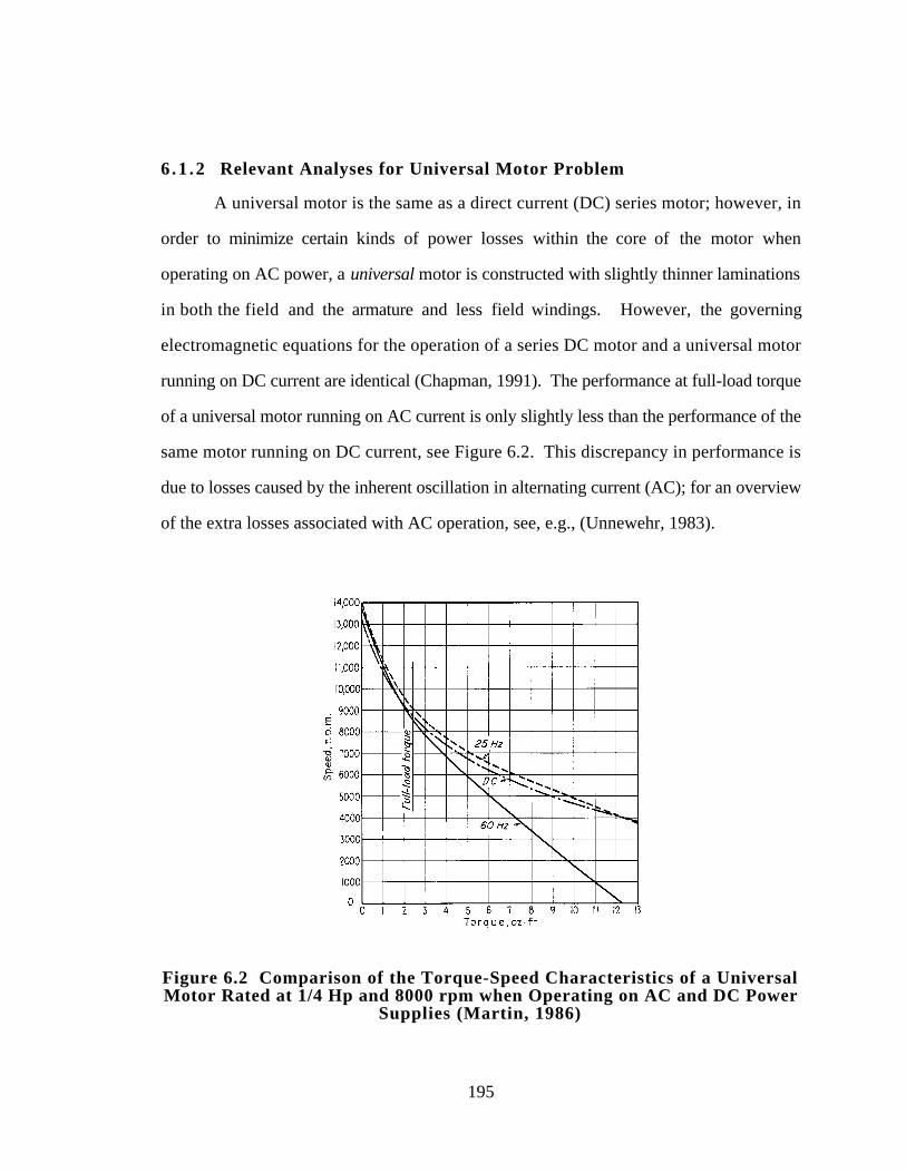
195
6 .1 .2 Relevant Analyses for Universal Motor Problem
A universal motor is the same as a direct current (DC) series motor; however, in
order to minimize certain kinds of power losses within the core of the motor when
operating on AC power, a universal motor is constructed with slightly thinner laminations
in both the field and the armature and less field windings. However, the governing
electromagnetic equations for the operation of a series DC motor and a universal motor
running on DC current are identical (Chapman, 1991). The performance at full-load torque
of a universal motor running on AC current is only slightly less than the performance of the
same motor running on DC current, see Figure 6.2. This discrepancy in performance is
due to losses caused by the inherent oscillation in alternating current (AC); for an overview
of the extra losses associated with AC operation, see, e.g., (Unnewehr, 1983).
Figure 6.2 Comparison of the Torque-Speed Characteristics of a UniversalMotor Rated at 1/4 Hp and 8000 rpm when Operating on AC and DC Power
Supplies (Martin, 1986)
196
These extra losses incurred in AC operation of a universal motor are difficult, if not
impossible, to model analytically; thus, complicated finite element analyses are becoming
more popular for modeling motor behavior under AC current. Since such a detailed
analysis is beyond the scope of this work, the derived model for the performance of the
universal motor is for DC operation for which simple analytical expressions are known or
can be derived. Moreover, several texts indicate that the performance of universal motors
under AC and DC conditions is quite comparable and include diagrams such as the one
reproduced in Figure 6.2 (see, e.g., (Chapman, 1991; Martin, 1986; Shultz, 1992;
Unnewehr, 1983); Shultz (1992) states that “Universal motors...will operate either on DC
or AC up to 60 Hz. Their performance will be essentially the same when operated on DC
or AC at 60 Hz.” The sample torque-speed curves in Figure 6.2 graphically illustrate this,
showing that for one specific motor, the performance characteristics between AC and DC
operation do not deviate significantly until well past the full-load torque of the motor. For
this work, all motors are designed for operation at full-load torque. Thus, it is assumed
that designing a universal motor under DC conditions yields satisfactory performance under
AC conditions as well.
The model takes as input the design variables {Nc, Ns, Awa, Awf, ro, t, lgap, I, Vt, L}
and returns as output the power (P), torque (T), mass (M), and efficiency (η) of the motor.
To formulate the model, it is necessary to derive equations for P, T, M, and η as functions
of the design variables. The equations are based primarily on those given in (Chapman,
1991) and (Cogdell, 1996) for DC electric motors unless otherwise noted.
Power
The basic equation for power output of a motor is the input power minus losses:
P = P in - Plosses [6.1]

197
where the input power is the product of the voltage and the current,
Pin = VtI [6.2]
and, for a universal motor, power is lost:
• in the copper wires as they heat-up (copper losses),
• at the interface between the brushes and the armature (brush losses),
• in the core due to hysteresis and eddy currents (core losses),
• in mechanical friction in the bearings supporting the rotor (mechanical losses),
• in heating up the core and copper wires which adversely effects the magnetic
properties of the core and the current carrying ability of the wires (thermal
losses), and
• due to stray losses (stray losses).
Simple analytic expressions only exist for the copper losses and the brush losses. Stray
losses usually are assumed to be no more than one percent, and thus can be neglected.
Mechanical losses can be minimized by an appropriate choice of bearing and housing
arrangement; however, these variables are beyond the scope of the motor model itself.
Hence mechanical losses are neglected. Core losses, especially those incurred by eddy
currents, can be minimized by the use of thin laminations in the stator and rotor; assuming
this is done, the core losses can be assumed to be small and thus can be neglected.
Thermal losses are in general non-negligible, but are highly dependent upon the external
cooling scheme (e.g., cooling fan and fins on the housing) applied to the motor. Because
an effective cooling scheme can keep the motor from running too hot, and as the setup of
the cooling configuration is beyond the scope of this model, thermal losses are neglected.
The combined effects of all the aforementioned neglected losses will, however, decrease
the output power and efficiency from the predicted value from the model. Nevertheless,
198
the following equations serve as a sufficiently accurate model for the DC operation of a
universal motor. Consequently, the general equation for power losses reduces from,
Plosses = Pcopper + Pbrush + Pthermal + Pcore + Pmechanical + Pstray [6.3]
to a more manageable:
Plosses = Pcopper + Pbrush [6.4]
where
Pcopper = I2(Ra + Rs) [6.5]
and
Pbrush = αI [6.6]
where α is typically 2 volts. Substituting these expressions into the power equation yields:
P = VtI-I2(Ra + Rs) - 2I [6.7]
However, Ra and Rs, the resistances of the armature and field windings, can be specified
further as functions of the design variables. The resistances Ra and Rs can be computed
directly from the general equation that the resistance of any wire is given by:
Resistance = (Resistivity)(Length)
Areacross −section
[6.8]
Assuming that each wrap (i.e., turn) of wire on the armature is approximately the shape of
a rectangle with length L (the stack length of the motor) and width lr (the diameter of the
armature) then in terms of the physical dimensions of the motor, lr can be expressed as two

199
times the radius of the armature, which is just the outer radius of the stator minus the
thickness of the stator minus the air gap length, or,
lr = 2(ro - t - lgap) [6.9]
so that the length of one wrap of wire on the armature is:
Lengthone wrap = 2L + 2lr = 2L + 4(ro - t - lgap) [6.10]
The total length of wire on the armature is the stack length, L, times the total number of
wraps on the armature, Nc, so that the resistance of the armature, Ra, is
Ra = ρ(2L + 4(r o−t − lgap))N c
A armature_wire
[6.11]
Similarly, assuming that each wrap of wire on the field is approximately the shape of a
rectangle with length L (the stack length of the motor) and width double the inner radius of
the stator (ro-t), then the resistance of the stator, Rs, is:
Rs = ρ(p field)(2L + 4(ro−t))Ns
A field_wire
[6.12]
However the purpose of the field windings is to create a magnetic field across the armature,
thus requiring two field poles, one for the “North” end of the magnetic field and one for the
“South” end. Thus, pfield is 2, and Equation 6.12 becomes Equation 6.13 which is:
Rs = ρ(2)(2L + 4(ro− t))N s
A field_wire
[6.13]
Now that Ra and Rs are expressed in terms of the design variables in Equations 6.11 and
6.13, the power equation is complete.
200
Efficiency
The equation for efficiency can be computed directly from the equation for power. The
basic equation for efficiency, expressed as a decimal and not a percentage, is given by:
η = P/Pin [6.14]
where P and Pin are given by Equations 6.2 and 6.7.
Mass
For the purpose of estimating the mass of the motor, it is modeled as a solid steel cylinder
with length L and radius lr/2 for the armature and a hollow steel cylinder with length L,
outer radius ro and inner radius (ro-t) for the stator. The mass of the windings on both the
armature and the field are also included, where the length of each winding is the same as
those assumed for the derivation of the power equation, see Equation 6.10. Thus the
equation for mass is of the form:
Mass = Mstator + Marmature + Mwindings [6.15]
where:
Mstator = π(ro2 - (ro - t)
2)(L)(ρsteel) [6.16]
Marmature = π(ro - t - lgap)2(L)(ρsteel) [6.17]
Mwindings = (Nc(2L + 4(ro - t - lgap))Awa + 2Ns(2L + 4(ro - t))Awf)ρcopper [6.18]
Using Equations 6.16-6.18 for Mstator, Marmature, and Mwindings, the mass of the motor,
Equation 6.15, can be estimated from the design variables.
Torque

201
The last equation to derive is an equation for torque. In general, the torque of a DC motor
is given by:
T = KφI [6.19]
where K is a motor constant, φ is the magnetic flux, and I is the current. For a DC motor,
K is computed as:
K = (Z)(parmature)
2πa[6.20]
where Z, the number of conductors on the armature, is:
Z = 2Nc [6.21]
and a, the number of current paths on the armature, is:
a = 2m = 2 [6.22]
assuming a simplex (m = 1) wave winding on the armature. Since the number of armature
poles on a universal motor is almost invariably two (cf., Martin, 1986), or,
parmature = 2 [6.23]
K can be reduced to:
K = 2N c(2)
2π(2) =
N c
π[6.24]
The derivation of the flux term, φ, is significantly more complicated. To begin,
consider the idealized DC motor shown in Figure 6.3a with its corresponding magnetic
circuit shown in Figure 6.3b. As shown in the figure, N is the number of turns on the

202
stator (which is equal to 2Ns for the model being derived), I is the current, A is the cross-
sectional area of the stator, lr is the diameter of the armature, lg is the gap length, and lc is
the mean magnetic path length in the stator.
(a) Physical model (b) Magnetic circuit
Figure 6.3 An Idealized DC Motor (Chapman, 1991)
In general the equation for flux through a magnetic circuit is simply the
magnetomotive force, ℑ, divided by the total reluctance of the circuit, ℜ:
φ =ℑℜ
[6.25]
where the magnetomotive force, ℑ, is simply the number of turns around one pole of the
field times the current:
ℑ = NsI [6.26]
203
The total reluctance, ℜ, is calculated from the magnetic circuit shown in Figure
6.3b. For a magnetic circuit, reluctances in series add just like resistors in series in an
electric circuit; therefore, the total reluctance in the idealized DC motor is the sum of the
reluctances of the stator, rotor, and two air gaps:
ℜ = ℜs + ℜr + 2ℜa [6.27]
where, in general, reluctance is calculated as:
ℜ = Length
(Permeability)(Area cross − section )[6.28]
When permeability, µ, is expressed as the relative permeability of the material times the
permeability of free space, µo, the reluctance of the stator, rotor, and air gaps are:
ℜs = l c
µ steelµoA s
, ℜr = l r
µ steelµoA r
, ℜa = l a
µ airµoAa
[6.29]
In order to approximate more closely a universal motor for this example, the
idealized DC motor geometry shown in Figure 6.3 is modified to be more representative of
a real universal motor. The resulting model geometry is shown in Figure 6.4a and is
described by the outer radius of the stator, ro, the thickness of the stator, t, the diameter of
the armature, lr, the length of the air gap, lgap, and the stack length, L. The resulting
magnetic circuit is shown in Figure 6.4b; notice that the magnetic circuit for the idealized
DC motor and the magnetic circuit for a universal motor are different, because in a
universal motor there are two paths which the magnetic flux can take around the stator, i.e.,
clockwise and counter-clockwise. These two paths are in parallel and thus are included in
the magnetic circuit as two parallel flux paths. Reluctances in parallel in a magnetic circuit
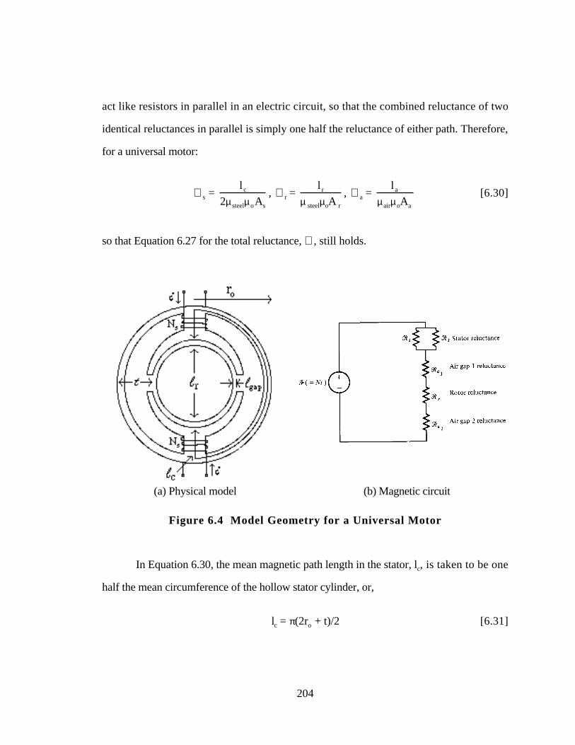
204
act like resistors in parallel in an electric circuit, so that the combined reluctance of two
identical reluctances in parallel is simply one half the reluctance of either path. Therefore,
for a universal motor:
ℜs = l c
2µ steelµoAs
, ℜr = l r
µ steelµoA r
, ℜa = l a
µ airµoAa
[6.30]
so that Equation 6.27 for the total reluctance, ℜ, still holds.
(a) Physical model (b) Magnetic circuit
Figure 6.4 Model Geometry for a Universal Motor
In Equation 6.30, the mean magnetic path length in the stator, lc, is taken to be one
half the mean circumference of the hollow stator cylinder, or,
lc = π(2ro + t)/2 [6.31]
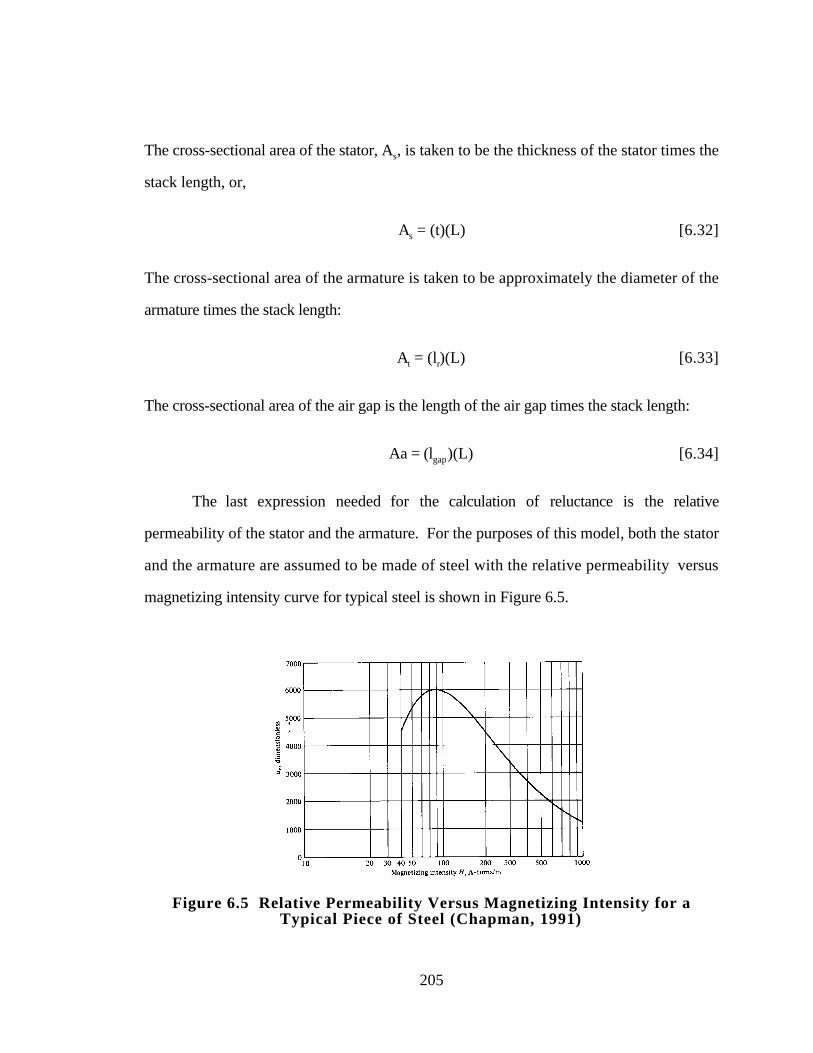
205
The cross-sectional area of the stator, As, is taken to be the thickness of the stator times the
stack length, or,
As = (t)(L) [6.32]
The cross-sectional area of the armature is taken to be approximately the diameter of the
armature times the stack length:
At = (lr)(L) [6.33]
The cross-sectional area of the air gap is the length of the air gap times the stack length:
Aa = (lgap)(L) [6.34]
The last expression needed for the calculation of reluctance is the relative
permeability of the stator and the armature. For the purposes of this model, both the stator
and the armature are assumed to be made of steel with the relative permeability versus
magnetizing intensity curve for typical steel is shown in Figure 6.5.
Figure 6.5 Relative Permeability Versus Magnetizing Intensity for aTypical Piece of Steel (Chapman, 1991)
206
The curve is divided into three regions, and each section is fit with an appropriate
numerical expression in order to include the curve shown in Figure 6.5 in the model. The
curve fits used are as follows:
µr = -0.2279H2 + 52.411H + 3115.8 H ≤ 220
µr = 11633.5 - 1486.33ln(H) 220 < H ≤ 1000
µr = 1000 H > 1000 [6.35]
where, from Ampere's Law, the magnetizing intensity, H, is given by,
H = N cI
l c + l r + 2lgap
[6.36]
The relative permeability of air, µair, is taken as unity, and the permeability of free space is a
constant, µo = 4 π 10-7. Now with expressions for K, φ, ℑ, ℜs, ℜr, ℜa, lc, lr, As, Ar, Aa,
and µsteel in terms of the design variables, the torque equation is complete.
This completes the mathematical model for the universal motor, and the PPCEM
now can be implemented to design a family of universal motors around a common product
platform. The initial steps of the PPCEM, Steps 1 and 2, are outlined in the next section.
6.2 STEPS 1 AND 2: CREATE MARKET SEGMENTATION GRID ANDCLASSIFY FACTORS FOR UNIVERSAL MOTOR PLATFORM
With a given set of performance requirements and the model derived in Section
6.1.3, the first step in implementing the PPCEM is to create the market segmentation grid
to identify and map which type of leveraging can be used to meet the overall design
requirements and realize the desired product platform and product family. The market
segmentation grid shown in Figure 6.6 depicts the desired leveraging strategy for this
universal motor example. The goal is to design a motor platform which can be leveraged
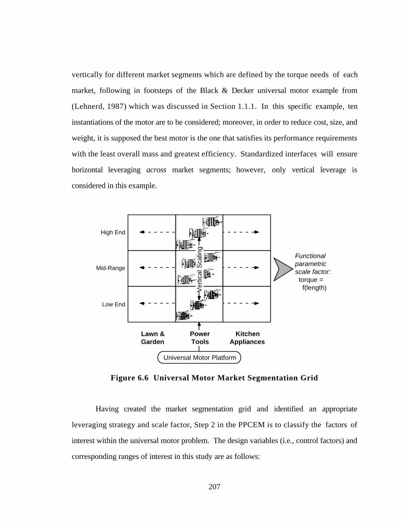
207
vertically for different market segments which are defined by the torque needs of each
market, following in footsteps of the Black & Decker universal motor example from
(Lehnerd, 1987) which was discussed in Section 1.1.1. In this specific example, ten
instantiations of the motor are to be considered; moreover, in order to reduce cost, size, and
weight, it is supposed the best motor is the one that satisfies its performance requirements
with the least overall mass and greatest efficiency. Standardized interfaces will ensure
horizontal leveraging across market segments; however, only vertical leverage is
considered in this example.
Low End
Mid-Range
High End
Functionalparametricscale factor: torque = f(length)
PowerTools
Universal Motor Platform
Ver
tical
Sca
ling
KitchenAppliances
Lawn &Garden
Figure 6.6 Universal Motor Market Segmentation Grid
Having created the market segmentation grid and identified an appropriate
leveraging strategy and scale factor, Step 2 in the PPCEM is to classify the factors of
interest within the universal motor problem. The design variables (i.e., control factors) and
corresponding ranges of interest in this study are as follows:
208
1. Number of turns of wire on the armature (100 ≤ Nc ≤ 1500 turns)
2. Number of turns of wire on each field pole (1 ≤ Ns ≤ 500 turns)
3. Cross-sectional area of the wire used on the armature (0.01 ≤ Awa ≤ 1.0 mm2)
4. Cross-sectional area of the wire used on the field poles (0.01 ≤ Awf ≤ 1.0 mm2)
5. Radius of the motor (0.01 ≤ ro ≤ 0.10 m)
6. Thickness of the stator (0.0005 ≤ t ≤ 0.10 m)
7. Current drawn by the motor (0.1 ≤ I ≤ 6.0 Amp)
The terminal voltage, Vt, is fixed at 115 volts to correspond to standard household
voltage, and the length of the air gap, lgap, is set to 0.7 mm which is taken to be the
minimum possible air gap length. The minimum air gap length is fixed because the
performance equations derived in Section 6.1.3 indicate that minimizing the air gap length
maximizes torque and minimizes mass with no effect on the other performance measures.
Following in the footsteps of the Black & Decker example, the stack length, L, is
the scale factor for the product family primarily because of its importance in the torque
equation, Equation 6.19, derived in Section 6.1.3, i.e., torque is directly proportional to
stack length. To increase torque across the platform, stack length of the motors is
increased while keeping the other physical parameters (e.g., the outer radius and the
thickness) unchanged. Furthermore, it is assumed that the greatest manufacturing costs
savings can be achieved by exploiting the fact that only the stack length of the motors varies
while still providing a variety of torque and power ratings. The initial range of interest for
stack length is taken to be 1 to 20 centimeters; specific instantiations are computed in Step 5
so as to meet the desired torque requirements for each platform derivative.
There are a total of six responses (i.e., goals and constraints) which are of interest
for each motor. The following constraint values—Table 6.2—and goal targets—Table
6.3—are assumed to define each market niche for each motor.
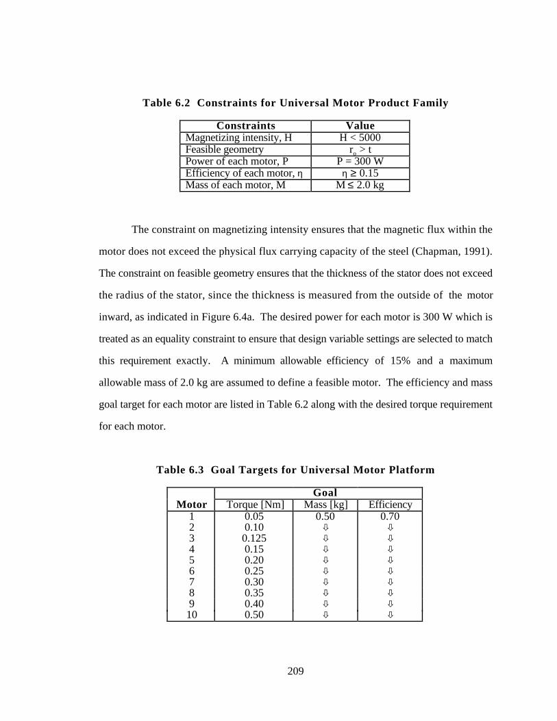
209
Table 6.2 Constraints for Universal Motor Product Family
Constraints ValueMagnetizing intensity, H H < 5000Feasible geometry ro > tPower of each motor, P P = 300 WEfficiency of each motor, η η ≥ 0.15Mass of each motor, M M ≤ 2.0 kg
The constraint on magnetizing intensity ensures that the magnetic flux within the
motor does not exceed the physical flux carrying capacity of the steel (Chapman, 1991).
The constraint on feasible geometry ensures that the thickness of the stator does not exceed
the radius of the stator, since the thickness is measured from the outside of the motor
inward, as indicated in Figure 6.4a. The desired power for each motor is 300 W which is
treated as an equality constraint to ensure that design variable settings are selected to match
this requirement exactly. A minimum allowable efficiency of 15% and a maximum
allowable mass of 2.0 kg are assumed to define a feasible motor. The efficiency and mass
goal target for each motor are listed in Table 6.2 along with the desired torque requirement
for each motor.
Table 6.3 Goal Targets for Universal Motor Platform
GoalMotor Torque [Nm] Mass [kg] Efficiency
1 0.05 0.50 0.702 0.10 ò ò3 0.125 ò ò4 0.15 ò ò5 0.20 ò ò6 0.25 ò ò7 0.30 ò ò8 0.35 ò ò9 0.40 ò ò10 0.50 ò ò
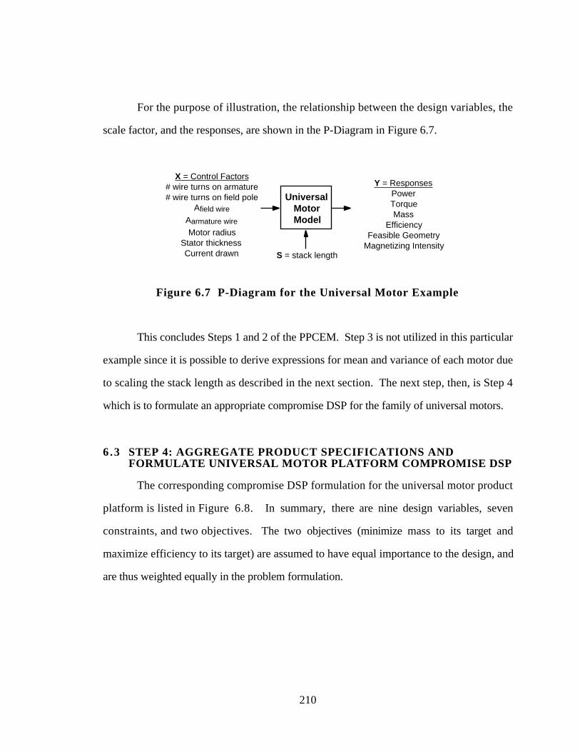
210
For the purpose of illustration, the relationship between the design variables, the
scale factor, and the responses, are shown in the P-Diagram in Figure 6.7.
X = Control Factors# wire turns on armature# wire turns on field pole
Afield wire
Aarmature wire
Motor radiusStator thicknessCurrent drawn
Y = ResponsesPowerTorqueMass
EfficiencyFeasible Geometry
Magnetizing Intensity S = stack length
UniversalMotorModel
Figure 6.7 P-Diagram for the Universal Motor Example
This concludes Steps 1 and 2 of the PPCEM. Step 3 is not utilized in this particular
example since it is possible to derive expressions for mean and variance of each motor due
to scaling the stack length as described in the next section. The next step, then, is Step 4
which is to formulate an appropriate compromise DSP for the family of universal motors.
6.3 STEP 4: AGGREGATE PRODUCT SPECIFICATIONS ANDFORMULATE UNIVERSAL MOTOR PLATFORM COMPROMISE DSP
The corresponding compromise DSP formulation for the universal motor product
platform is listed in Figure 6.8. In summary, there are nine design variables, seven
constraints, and two objectives. The two objectives (minimize mass to its target and
maximize efficiency to its target) are assumed to have equal importance to the design, and
are thus weighted equally in the problem formulation.
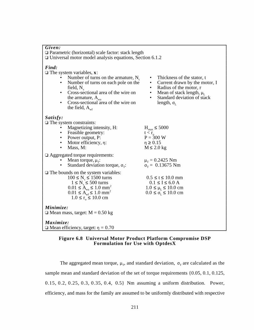
211
Given:q Parametric (horizontal) scale factor: stack lengthq Universal motor model analysis equations, Section 6.1.2
Find:q The system variables, x:
• Number of turns on the armature, Nc • Thickness of the stator, t• Number of turns on each pole on the
field, Ns
• Current drawn by the motor, I• Radius of the motor, r
• Cross-sectional area of the wire onthe armature, Awa
• Mean of stack length, µL• Standard deviation of stack
• Cross-sectional area of the wire onthe field, Awf
length, σL
Satisfy:q The system constraints:
• Magnetizing intensity, H: Hmax ≤ 5000• Feasible geometry: t < ro• Power output, P: P = 300 W• Motor efficiency, η: η ≥ 0.15• Mass, M: M ≤ 2.0 kg
q Aggregated torque requirements:• Mean torque, µT: µT = 0.2425 Nm• Standard deviation torque, σT: σT = 0.13675 Nm
q The bounds on the system variables:100 ≤ Nc ≤ 1500 turns 0.5 ≤ t ≤ 10.0 mm
1 ≤ Ns ≤ 500 turns 0.1 ≤ I ≤ 6.0 A0.01 ≤ Awa ≤ 1.0 mm2 1.0 ≤ µL ≤ 10.0 cm0.01 ≤ Awf ≤ 1.0 mm2 0.0 ≤ σL ≤ 10.0 cm
1.0 ≤ ro ≤ 10.0 cm
Minimize:q Mean mass, target: M = 0.50 kg
Maximize:q Mean efficiency, target: η = 0.70
Figure 6.8 Universal Motor Product Platform Compromise DSPFormulation for Use with OptdesX
The aggregated mean torque, µT, and standard deviation, σT are calculated as the
sample mean and standard deviation of the set of torque requirements {0.05, 0.1, 0.125,
0.15, 0.2, 0.25, 0.3, 0.35, 0.4, 0.5} Nm assuming a uniform distribution. Power,
efficiency, and mass for the family are assumed to be uniformly distributed with respective
212
means and standard deviations because it is assumed that the distribution of the demand for
the motors is uniform.
The mean power, mean efficiency, and mean mass are calculated as the power,
efficiency, and mass, respectively, for the mean length. The standard deviation of torque is
approximated using a first-order Taylor series expansion, assuming that the standard
deviation is small (Phadke, 1989):
σT ˙ = ∂T
∂µL
σ L [6.37]
Now that the compromise DSP for the family of universal motors is formulated, Step 5 of
the PPCEM is executed to develop the universal motor platform.
6.4 STEP 5: DEVELOP THE UNIVERSAL MOTOR PLATFORM
For this example problem, the compromise DSP formulated in Section 6.3 is solved
using the Generalized Reduced Gradient (GRG) algorithm in OptdesX. For a thorough
explanation of OptdesX and the GRG algorithm, see, e.g., (Parkinson, et al., 1998). The
OptdesX software package is used instead of DSIDES in this example since implementation
of the PPCEM is not algorithm dependent.
Note that in order to develop the product portfolio, the compromise DSP is
formulated with goals for mean torque, µT, and standard deviation of torque, σT, which
ensures that the product portfolio will be able to be instantiated for all ten values of torque
within the range of the scale factor specified by the mean and standard deviation, µL and σL,
for the stack length. Also note that the constraint on magnetizing intensity is formulated to
ensure that the entire product family will meet the constraint on magnetizing intensity
individually. This is accomplished by computing a maximum magnetizing intensity which
represents the magnetizing intensity for the largest instantiation of the product family and is
simply evaluated at the upper bound of current. The compromise DSP in Figure 6.8 is
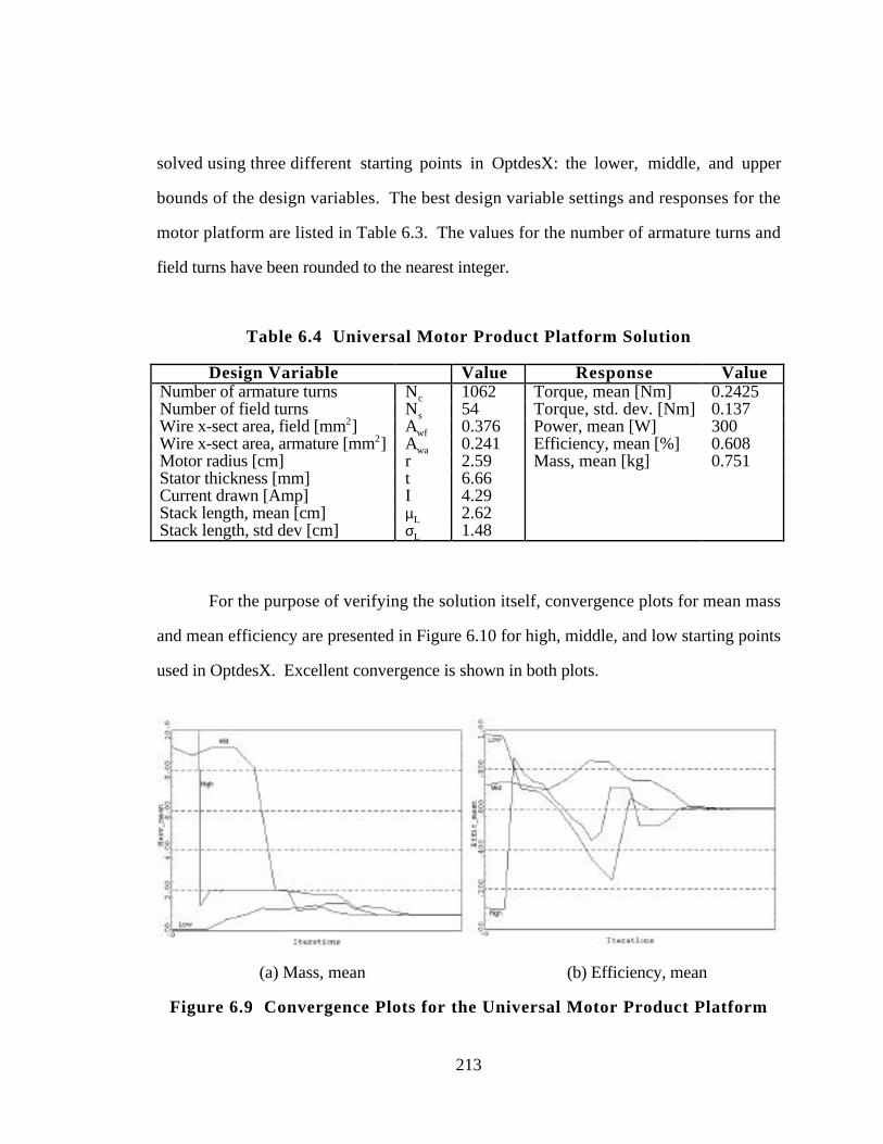
213
solved using three different starting points in OptdesX: the lower, middle, and upper
bounds of the design variables. The best design variable settings and responses for the
motor platform are listed in Table 6.3. The values for the number of armature turns and
field turns have been rounded to the nearest integer.
Table 6.4 Universal Motor Product Platform Solution
Design Variable Value Response ValueNumber of armature turns Nc 1062 Torque, mean [Nm] 0.2425Number of field turns Ns 54 Torque, std. dev. [Nm] 0.137Wire x-sect area, field [mm2] Awf 0.376 Power, mean [W] 300Wire x-sect area, armature [mm2] Awa 0.241 Efficiency, mean [%] 0.608Motor radius [cm] r 2.59 Mass, mean [kg] 0.751Stator thickness [mm] t 6.66Current drawn [Amp] I 4.29Stack length, mean [cm] µL 2.62Stack length, std dev [cm] σL 1.48
For the purpose of verifying the solution itself, convergence plots for mean mass
and mean efficiency are presented in Figure 6.10 for high, middle, and low starting points
used in OptdesX. Excellent convergence is shown in both plots.
(a) Mass, mean (b) Efficiency, mean
Figure 6.9 Convergence Plots for the Universal Motor Product Platform
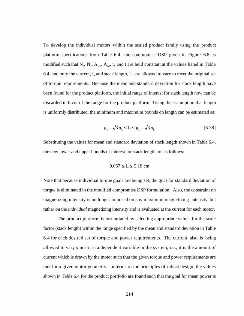
214
To develop the individual motors within the scaled product family using the product
platform specifications from Table 6.4, the compromise DSP given in Figure 6.8 is
modified such that Nc, Ns, Awa, Awf, r, and t are held constant at the values listed in Table
6.4, and only the current, I, and stack length, L, are allowed to vary to meet the original set
of torque requirements. Because the mean and standard deviation for stack length have
been found for the product platform, the initial range of interest for stack length now can be
discarded in favor of the range for the product platform. Using the assumption that length
is uniformly distributed, the minimum and maximum bounds on length can be estimated as:
µL - 3 σL ≤ L ≤ µL - 3 σL [6.38]
Substituting the values for mean and standard deviation of stack length shown in Table 6.4,
the new lower and upper bounds of interest for stack length are as follows:
0.057 ≤ L ≤ 5.18 cm
Note that because individual torque goals are being set, the goal for standard deviation of
torque is eliminated in the modified compromise DSP formulation. Also, the constraint on
magnetizing intensity is no longer imposed on any maximum magnetizing intensity but
rather on the individual magnetizing intensity and is evaluated at the current for each motor.
The product platform is instantiated by selecting appropriate values for the scale
factor (stack length) within the range specified by the mean and standard deviation in Table
6.4 for each desired set of torque and power requirements. The current also is being
allowed to vary since it is a dependent variable in the system, i.e., it is the amount of
current which is drawn by the motor such that the given torque and power requirements are
met for a given motor geometry. In terms of the principles of robust design, the values
shown in Table 6.4 for the product portfolio are found such that the goal for mean power is
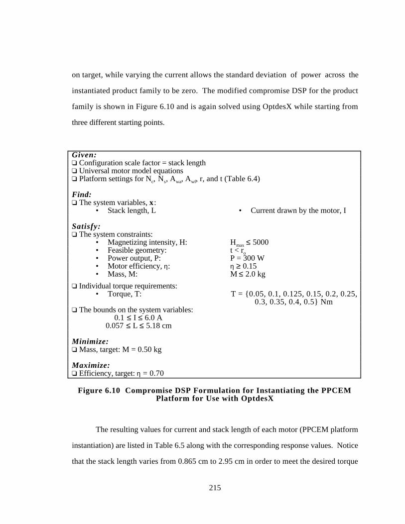
215
on target, while varying the current allows the standard deviation of power across the
instantiated product family to be zero. The modified compromise DSP for the product
family is shown in Figure 6.10 and is again solved using OptdesX while starting from
three different starting points.
Given:q Configuration scale factor = stack lengthq Universal motor model equationsq Platform settings for Nc, Ns, Awa, Awf, r, and t (Table 6.4)
Find:q The system variables, x:
• Stack length, L • Current drawn by the motor, I
Satisfy:q The system constraints:
• Magnetizing intensity, H: Hmax ≤ 5000• Feasible geometry: t < ro• Power output, P: P = 300 W• Motor efficiency, η: η ≥ 0.15• Mass, M: M ≤ 2.0 kg
q Individual torque requirements:• Torque, T: T = {0.05, 0.1, 0.125, 0.15, 0.2, 0.25,
0.3, 0.35, 0.4, 0.5} Nmq The bounds on the system variables:
0.1 ≤ I ≤ 6.0 A0.057 ≤ L ≤ 5.18 cm
Minimize:q Mass, target: M = 0.50 kg
Maximize:q Efficiency, target: η = 0.70
Figure 6.10 Compromise DSP Formulation for Instantiating the PPCEMPlatform for Use with OptdesX
The resulting values for current and stack length of each motor (PPCEM platform
instantiation) are listed in Table 6.5 along with the corresponding response values. Notice
that the stack length varies from 0.865 cm to 2.95 cm in order to meet the desired torque
216
and power requirements. The resulting current drawn by the system ranges from 3.39
Amps to 5.82 Amps which is slightly high but acceptable for a motor with such a large
torque. Finally, notice that only three motors meet the desired efficiency target of 70%,
and these are all at the low-end, and only one motor achieves the mass target of 0.5 kg.
Table 6.5 Universal Motor Product Family PPCEM Instantiations
Product Specifications (Design Variables) ResponsesAwf Awa I r t L T P η M
Motor Nc Ns [mm2] [mm2] [Amp] [cm] [mm] [cm] [Nm] [W] [%] [kg]1 1062 54 0.376 0.241 3.39 2.59 6.66 0.865 0.05 300 76.8 0.3802 ò ò ò ò 3.62 ò ò 1.53 0.10 ò 72.2 0.5203 ò ò ò ò 3.73 ò ò 1.79 0.125 ò 70.0 0.5764 ò ò ò ò 3.85 ò ò 2.02 0.15 ò 67.9 0.6255 ò ò ò ò 4.08 ò ò 2.39 0.20 ò 63.9 0.7036 ò ò ò ò 4.33 ò ò 2.66 0.25 ò 60.2 0.7597 ò ò ò ò 4.59 ò ò 2.83 0.30 ò 56.8 0.7978 ò ò ò ò 4.87 ò ò 2.94 0.35 ò 53.6 0.8209 ò ò ò ò 5.16 ò ò 2.99 0.40 ò 50.5 0.83010 ò ò ò ò 5.82 ò ò 2.95 0.50 ò 44.8 0.820
It is uncertain whether the failure to achieve the desired mass and efficiency targets
is a property of the system itself or a result of using the PPCEM. Therefore, a family of
individually designed universal motors is developed in the next section to provide a
benchmark for comparison. The differences between this family of benchmark motors and
the PPCEM instantiations are then compared to verify the PPCEM solutions.
6.5 RAMIFICATIONS OF THE RESULTS OF THE ELECTRIC MOTOREXAMPLE PROBLEM
6.5 .1 Development of a Benchmark Universal Motor Family
In order to generate a family of benchmark motors to compare with the PPCEM
family of motors, the compromise DSP presented in Figure 6.10 is modified such that Nc,
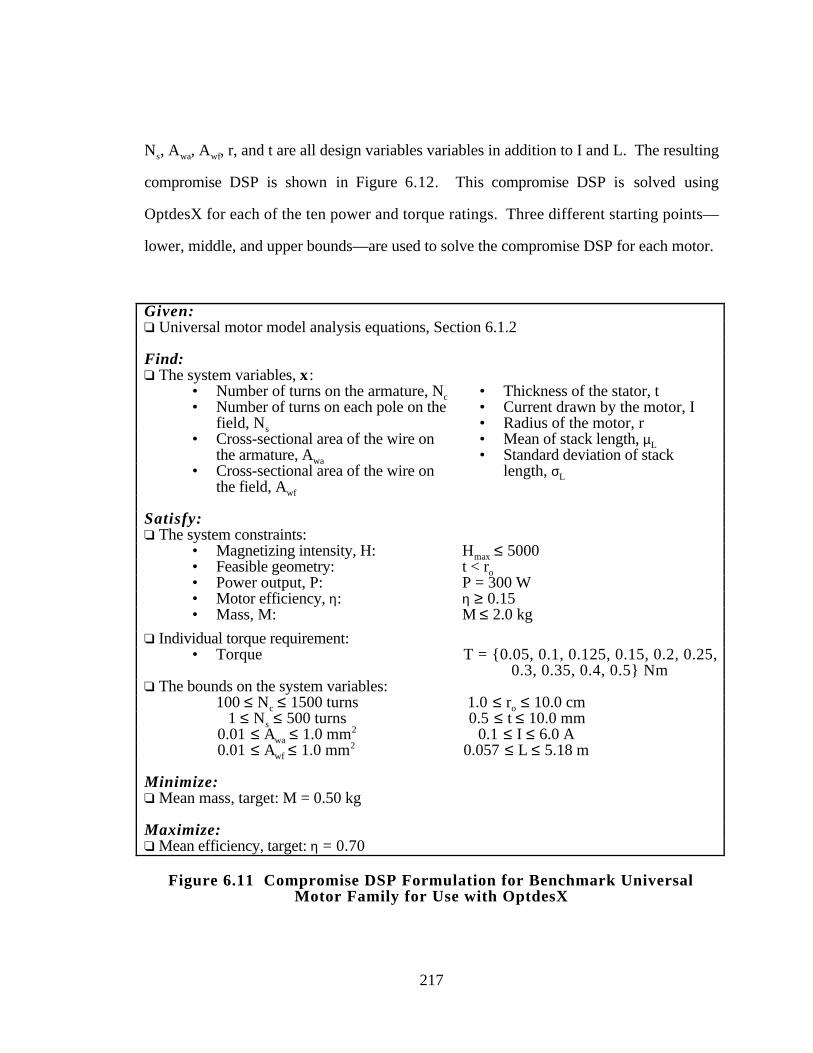
217
Ns, Awa, Awf, r, and t are all design variables variables in addition to I and L. The resulting
compromise DSP is shown in Figure 6.12. This compromise DSP is solved using
OptdesX for each of the ten power and torque ratings. Three different starting points—
lower, middle, and upper bounds—are used to solve the compromise DSP for each motor.
Given:q Universal motor model analysis equations, Section 6.1.2
Find:q The system variables, x:
• Number of turns on the armature, Nc • Thickness of the stator, t• Number of turns on each pole on the
field, Ns
• Current drawn by the motor, I• Radius of the motor, r
• Cross-sectional area of the wire onthe armature, Awa
• Mean of stack length, µL• Standard deviation of stack
• Cross-sectional area of the wire onthe field, Awf
length, σL
Satisfy:q The system constraints:
• Magnetizing intensity, H: Hmax ≤ 5000• Feasible geometry: t < ro• Power output, P: P = 300 W• Motor efficiency, η: η ≥ 0.15• Mass, M: M ≤ 2.0 kg
q Individual torque requirement:• Torque T = {0.05, 0.1, 0.125, 0.15, 0.2, 0.25,
0.3, 0.35, 0.4, 0.5} Nmq The bounds on the system variables:
100 ≤ Nc ≤ 1500 turns 1.0 ≤ ro ≤ 10.0 cm1 ≤ Ns ≤ 500 turns 0.5 ≤ t ≤ 10.0 mm
0.01 ≤ Awa ≤ 1.0 mm2 0.1 ≤ I ≤ 6.0 A0.01 ≤ Awf ≤ 1.0 mm2 0.057 ≤ L ≤ 5.18 m
Minimize:q Mean mass, target: M = 0.50 kg
Maximize:q Mean efficiency, target: η = 0.70
Figure 6.11 Compromise DSP Formulation for Benchmark UniversalMotor Family for Use with OptdesX
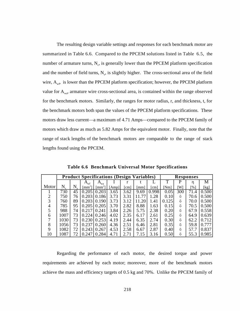
218
The resulting design variable settings and responses for each benchmark motor are
summarized in Table 6.6. Compared to the PPCEM solutions listed in Table 6.5, the
number of armature turns, Nc, is generally lower than the PPCEM platform specification
and the number of field turns, Ns, is slightly higher. The cross-sectional area of the field
wire, Awf, is lower than the PPCEM platform specification; however, the PPCEM platform
value for Awa, armature wire cross-sectional area, is contained within the range observed
for the benchmark motors. Similarly, the ranges for motor radius, r, and thickness, t, for
the benchmark motors both span the values of the PPCEM platform specifications. These
motors draw less current—a maximum of 4.71 Amps—compared to the PPCEM family of
motors which draw as much as 5.82 Amps for the equivalent motor. Finally, note that the
range of stack lengths of the benchmark motors are comparable to the range of stack
lengths found using the PPCEM.
Table 6.6 Benchmark Universal Motor Specifications
Product Specifications (Design Variables) ResponsesAwf Awa I r t L T P η M
Motor Nc Ns [mm2] [mm2] [Amp] [cm] [mm] [cm] [Nm] [W] [%] [kg]1 730 45 0.205 0.203 3.65 3.62 9.69 0.998 0.05 300 71.4 0.5002 750 76 0.203 0.186 3.73 3.31 11.77 1.28 0.10 ò 70.6 0.5003 760 89 0.203 0.190 3.73 3.12 11.20 1.41 0.125 ò 70.0 0.5004 785 95 0.205 0.205 3.70 2.82 8.88 1.63 0.15 ò 70.5 0.5005 988 74 0.217 0.241 3.84 2.26 5.75 2.38 0.20 ò 67.9 0.5586 1007 73 0.224 0.246 4.02 2.35 6.17 2.61 0.25 ò 64.9 0.6397 1030 73 0.230 0.253 4.19 2.44 6.35 2.74 0.30 ò 62.2 0.7128 1056 73 0.237 0.260 4.36 2.51 6.46 2.81 0.35 ò 59.8 0.7779 1082 72 0.243 0.267 4.53 2.58 6.67 2.87 0.40 ò 57.7 0.83710 1087 72 0.247 0.284 4.71 2.71 7.15 3.16 0.50 ò 55.3 0.985
Regarding the performance of each motor, the desired torque and power
requirements are achieved by each motor; moreover, more of the benchmark motors
achieve the mass and efficiency targets of 0.5 kg and 70%. Unlike the PPCEM family of
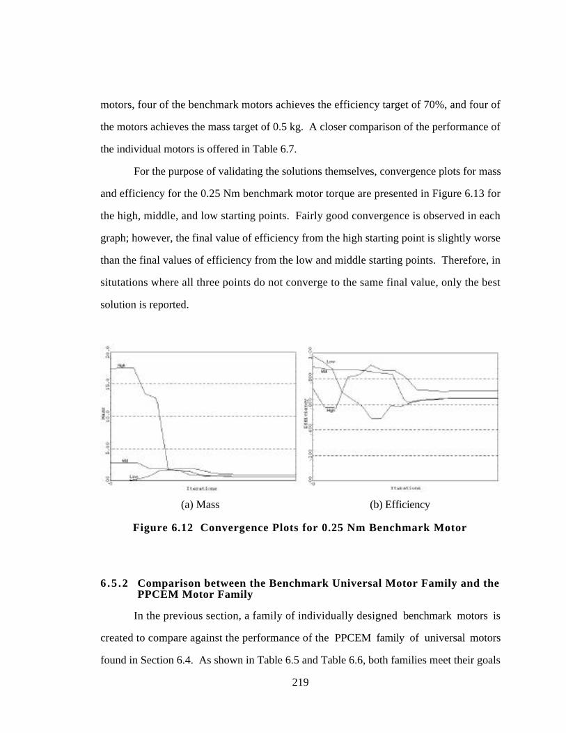
219
motors, four of the benchmark motors achieves the efficiency target of 70%, and four of
the motors achieves the mass target of 0.5 kg. A closer comparison of the performance of
the individual motors is offered in Table 6.7.
For the purpose of validating the solutions themselves, convergence plots for mass
and efficiency for the 0.25 Nm benchmark motor torque are presented in Figure 6.13 for
the high, middle, and low starting points. Fairly good convergence is observed in each
graph; however, the final value of efficiency from the high starting point is slightly worse
than the final values of efficiency from the low and middle starting points. Therefore, in
situtations where all three points do not converge to the same final value, only the best
solution is reported.
(a) Mass (b) Efficiency
Figure 6.12 Convergence Plots for 0.25 Nm Benchmark Motor
6 .5 .2 Comparison between the Benchmark Universal Motor Family and thePPCEM Motor Family
In the previous section, a family of individually designed benchmark motors is
created to compare against the performance of the PPCEM family of universal motors
found in Section 6.4. As shown in Table 6.5 and Table 6.6, both families meet their goals
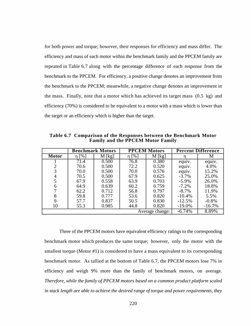
220
for both power and torque; however, their responses for efficiency and mass differ. The
efficiency and mass of each motor within the benchmark family and the PPCEM family are
repeated in Table 6.7 along with the percentage difference of each response from the
benchmark to the PPCEM. For efficiency, a positive change denotes an improvement from
the benchmark to the PPCEM; meanwhile, a negative change denotes an improvement in
the mass. Finally, note that a motor which has achieved its target mass (0.5 kg) and
efficiency (70%) is considered to be equivalent to a motor with a mass which is lower than
the target or an efficiency which is higher than the target.
Table 6.7 Comparison of the Responses between the Benchmark MotorFamily and the PPCEM Motor Family
Benchmark Motors PPCEM Motors Percent DifferenceMotor η [%] M [kg] η [%] M [kg] η M
1 71.4 0.500 76.8 0.380 equiv. equiv.2 70.6 0.500 72.2 0.520 equiv. 4.0%3 70.0 0.500 70.0 0.576 equiv. 15.2%4 70.5 0.500 67.9 0.625 -3.7% 25.0%5 67.9 0.558 63.9 0.703 -5.9% 26.0%6 64.9 0.639 60.2 0.759 -7.2% 18.8%7 62.2 0.712 56.8 0.797 -8.7% 11.9%8 59.8 0.777 53.6 0.820 -10.4% 5.5%9 57.7 0.837 50.5 0.830 -12.5% -0.8%10 55.3 0.985 44.8 0.820 -19.0% -16.7%
Average change: -6.74% 8.89%
Three of the PPCEM motors have equivalent efficiency ratings to the corresponding
benchmark motor which produces the same torque; however, only the motor with the
smallest torque (Motor #1) is considered to have a mass equivalent to its corresponding
benchmark motor. As tallied at the bottom of Table 6.7, the PPCEM motors lose 7% in
efficiency and weigh 9% more than the family of benchmark motors, on average.
Therefore, while the family of PPCEM motors based on a common product platform scaled
in stack length are able to achieve the desired range of torque and power requirements, they
221
lose, on average, 10% in both efficiency and mass compared to an equivalent family of
individually designed benchmark motors. At this point, it is up to the judgment of the
engineering designers and managers to decide if the savings (in inventory, manufacturing,
etc.) from having a family motors based a common platform and scaled only in stack length
outweighs the sacrifice in mass and efficiency. Meanwhile, an attempt to improve the
performance of the PPCEM family of motors in relation to the benchmark family of motors
is offered in the next section.
6 .5 .3 Improvements to the PPCEM Motor Family and Lessons Learned
While investigating this example, it was learned that Black & Decker varies more
than just stack length when it scales its universal motors to meet a variety of power ratings.
In addition to increasing the stack length of the motor, they also allow the number of turns
in the field and armature and the cross-sectional area of the wires in the field and armature
to vary from one motor to the next. Careful inspection of any two motors from one of their
power tool lines (say, corded drills) reveals that this is indeed the case.
The question then becomes: how well do the PPCEM instantiations perform if the
number of field and armature turns (Ns and Nc) and the cross-sectional area of the field and
armature wires (Awf and Awa) are allowed to vary in conjunction with varying the stack
length (and current)? The results obtained by solving a new set of compromise DSPs for
each universal motor are listed in Table 6.8. These solutions are obtained by modifying the
compromise DSP in Figure 6.10 to allow Nc, Ns, Awf, and Awa to vary from their platform
settings of 1062, 54, 0.376 mm2, and 0.241 mm2, respectively.
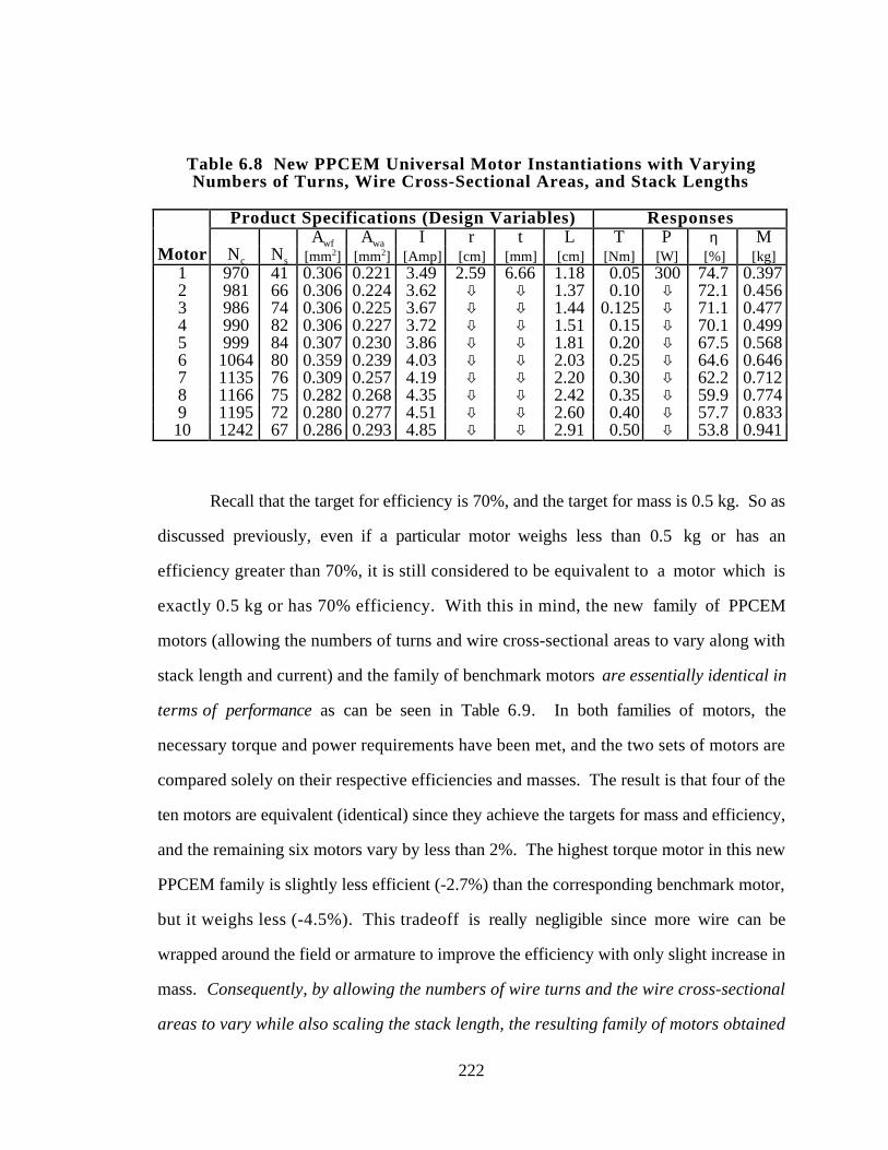
222
Table 6.8 New PPCEM Universal Motor Instantiations with VaryingNumbers of Turns, Wire Cross-Sectional Areas, and Stack Lengths
Product Specifications (Design Variables) ResponsesAwf Awa I r t L T P η M
Motor Nc Ns [mm2] [mm2] [Amp] [cm] [mm] [cm] [Nm] [W] [%] [kg]1 970 41 0.306 0.221 3.49 2.59 6.66 1.18 0.05 300 74.7 0.3972 981 66 0.306 0.224 3.62 ò ò 1.37 0.10 ò 72.1 0.4563 986 74 0.306 0.225 3.67 ò ò 1.44 0.125 ò 71.1 0.4774 990 82 0.306 0.227 3.72 ò ò 1.51 0.15 ò 70.1 0.4995 999 84 0.307 0.230 3.86 ò ò 1.81 0.20 ò 67.5 0.5686 1064 80 0.359 0.239 4.03 ò ò 2.03 0.25 ò 64.6 0.6467 1135 76 0.309 0.257 4.19 ò ò 2.20 0.30 ò 62.2 0.7128 1166 75 0.282 0.268 4.35 ò ò 2.42 0.35 ò 59.9 0.7749 1195 72 0.280 0.277 4.51 ò ò 2.60 0.40 ò 57.7 0.83310 1242 67 0.286 0.293 4.85 ò ò 2.91 0.50 ò 53.8 0.941
Recall that the target for efficiency is 70%, and the target for mass is 0.5 kg. So as
discussed previously, even if a particular motor weighs less than 0.5 kg or has an
efficiency greater than 70%, it is still considered to be equivalent to a motor which is
exactly 0.5 kg or has 70% efficiency. With this in mind, the new family of PPCEM
motors (allowing the numbers of turns and wire cross-sectional areas to vary along with
stack length and current) and the family of benchmark motors are essentially identical in
terms of performance as can be seen in Table 6.9. In both families of motors, the
necessary torque and power requirements have been met, and the two sets of motors are
compared solely on their respective efficiencies and masses. The result is that four of the
ten motors are equivalent (identical) since they achieve the targets for mass and efficiency,
and the remaining six motors vary by less than 2%. The highest torque motor in this new
PPCEM family is slightly less efficient (-2.7%) than the corresponding benchmark motor,
but it weighs less (-4.5%). This tradeoff is really negligible since more wire can be
wrapped around the field or armature to improve the efficiency with only slight increase in
mass. Consequently, by allowing the numbers of wire turns and the wire cross-sectional
areas to vary while also scaling the stack length, the resulting family of motors obtained
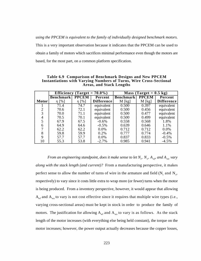
223
using the PPCEM is equivalent to the family of individually designed benchmark motors.
This is a very important observation because it indicates that the PPCEM can be used to
obtain a family of motors which sacrifices minimal performance even though the motors are
based, for the most part, on a common platform specification.
Table 6.9 Comparison of Benchmark Designs and New PPCEMInstantiations with Varying Numbers of Turns, Wire Cross-Sectional
Areas, and Stack Lengths
Efficiency (Target = 70.0%) Mass (Target = 0.5 kg)Benchmark PPCEM Percent Benchmark PPCEM Percent
Motor η [%] η [%] Difference M [kg] M [kg] Difference1 71.4 74.7 equivalent 0.500 0.397 equivalent2 70.6 72.1 equivalent 0.500 0.456 equivalent3 70.0 71.1 equivalent 0.500 0.477 equivalent4 70.5 70.1 equivalent 0.500 0.499 equivalent5 67.9 67.5 -0.6% 0.558 0.568 1.8%6 64.9 64.6 -0.5% 0.639 0.646 1.1%7 62.2 62.2 0.0% 0.712 0.712 0.0%8 59.8 59.9 0.2% 0.777 0.774 -0.4%9 57.7 57.7 0.0% 0.837 0.833 -0.5%10 55.3 53.8 -2.7% 0.985 0.941 -4.5%
From an engineering standpoint, does it make sense to let Nc, Ns, Awf, and Awa vary
along with the stack length (and current)? From a manufacturing perspective, it makes
perfect sense to allow the number of turns of wire in the armature and field (Nc and Ns,
respectively) to vary since it costs little extra to wrap more (or fewer) turns when the motor
is being produced. From a inventory perspective, however, it would appear that allowing
Awf and Awa to vary is not cost effective since it requires that multiple wire types (i.e.,
varying cross-sectional areas) must be kept in stock in order to produce the family of
motors. The justification for allowing Awf and Awa to vary is as follows. As the stack
length of the motor increases (with everything else being held constant), the torque on the
motor increases; however, the power output actually decreases because the copper losses,
224
given by Equation 6.5, increase as since Ra and Rs increase (see Equation 6.8) as stack
length increases.
One way to compensate for this loss in power is to allow more current to be drawn
as is the case in this example. What is typically done, however, to compensate for this
decrease in power (as the stack length is increased) is to decrease the number of field and
armature turns while simultaneously increasing the field and armature wire cross-sectional
areas. This lowers the resistances Ra and Rs and reduces copper losses without having to
draw additional current in order to maintain the desired output power. An added benefit of
this approach is that the rotational speed of the motor will also increase. In reality, the
operating speed of the motor is a very important design consideration since power and
torque are related through the equation:
P = Tω [6.39]
where P is power, T is torque, and ω is the rotational speed of the motor. The speed of the
motor has been neglected in this example since it is fixed once power and torque have been
specified. Based on Equation 6.39, for a fixed power output, as torque increases, the
rotational speed of the motor must decrease. In many cases however, as power increases
and torque increases, maintaining a consistent operating speed for the motor is often
desired. The additional inventory costs incurred by stocking a wider variety of wire sizes
is offset by this combination of effects.
But what if Awf and Awa were held fixed and only Nc and Ns were allowed to vary
along with stack length (and current)? The answer is summarized in Table 6.10 wherein
the compromise DSP for the family of motors for instantiating the PPCEM platform,
Figure 6.10, has been modified a third time to allow only Nc, Ns, L and I to vary from the
platform specifications. Comparison of the data in Table 6.10 with Table 6.8 (the PPCEM
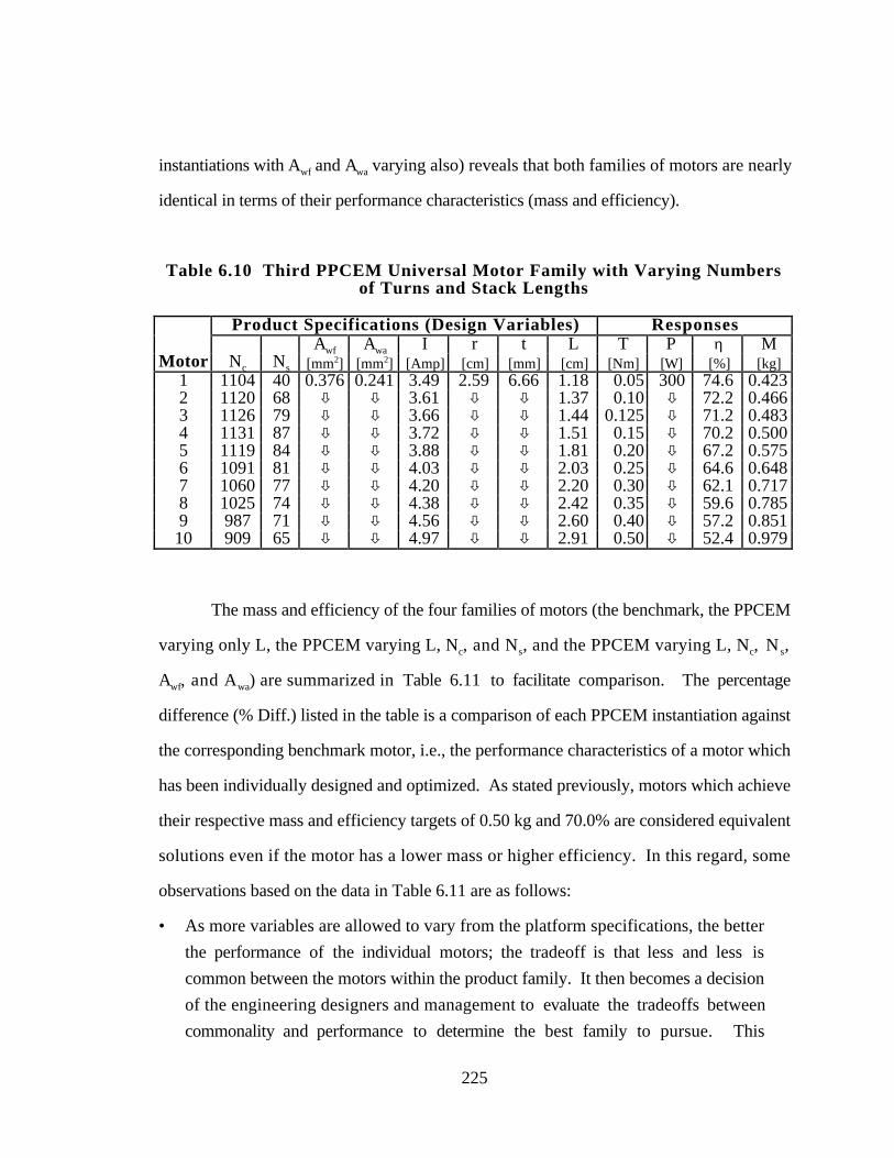
225
instantiations with Awf and Awa varying also) reveals that both families of motors are nearly
identical in terms of their performance characteristics (mass and efficiency).
Table 6.10 Third PPCEM Universal Motor Family with Varying Numbersof Turns and Stack Lengths
Product Specifications (Design Variables) ResponsesAwf Awa I r t L T P η M
Motor Nc Ns [mm2] [mm2] [Amp] [cm] [mm] [cm] [Nm] [W] [%] [kg]1 1104 40 0.376 0.241 3.49 2.59 6.66 1.18 0.05 300 74.6 0.4232 1120 68 ò ò 3.61 ò ò 1.37 0.10 ò 72.2 0.4663 1126 79 ò ò 3.66 ò ò 1.44 0.125 ò 71.2 0.4834 1131 87 ò ò 3.72 ò ò 1.51 0.15 ò 70.2 0.5005 1119 84 ò ò 3.88 ò ò 1.81 0.20 ò 67.2 0.5756 1091 81 ò ò 4.03 ò ò 2.03 0.25 ò 64.6 0.6487 1060 77 ò ò 4.20 ò ò 2.20 0.30 ò 62.1 0.7178 1025 74 ò ò 4.38 ò ò 2.42 0.35 ò 59.6 0.7859 987 71 ò ò 4.56 ò ò 2.60 0.40 ò 57.2 0.85110 909 65 ò ò 4.97 ò ò 2.91 0.50 ò 52.4 0.979
The mass and efficiency of the four families of motors (the benchmark, the PPCEM
varying only L, the PPCEM varying L, Nc, and Ns, and the PPCEM varying L, Nc, N s,
Awf, and Awa) are summarized in Table 6.11 to facilitate comparison. The percentage
difference (% Diff.) listed in the table is a comparison of each PPCEM instantiation against
the corresponding benchmark motor, i.e., the performance characteristics of a motor which
has been individually designed and optimized. As stated previously, motors which achieve
their respective mass and efficiency targets of 0.50 kg and 70.0% are considered equivalent
solutions even if the motor has a lower mass or higher efficiency. In this regard, some
observations based on the data in Table 6.11 are as follows:
• As more variables are allowed to vary from the platform specifications, the better
the performance of the individual motors; the tradeoff is that less and less is
common between the motors within the product family. It then becomes a decision
of the engineering designers and management to evaluate the tradeoffs between
commonality and performance to determine the best family to pursue. This
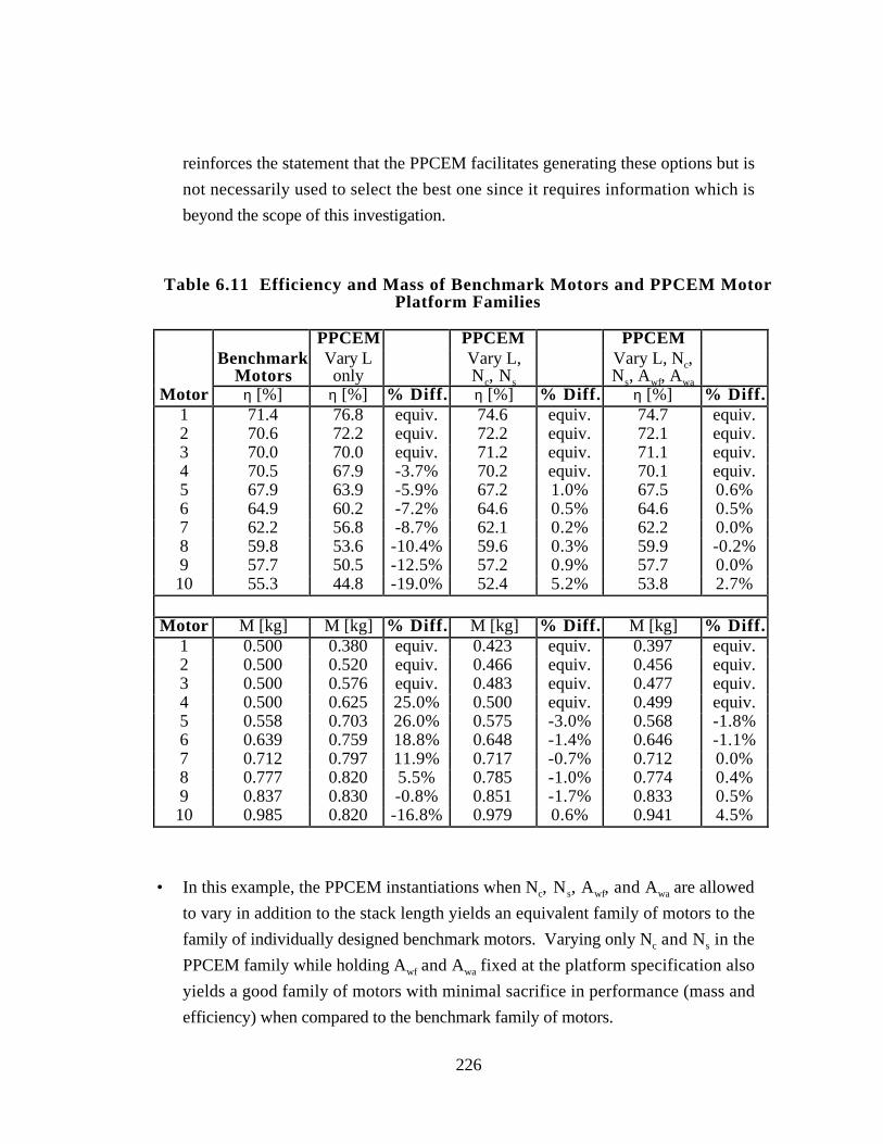
226
reinforces the statement that the PPCEM facilitates generating these options but is
not necessarily used to select the best one since it requires information which is
beyond the scope of this investigation.
Table 6.11 Efficiency and Mass of Benchmark Motors and PPCEM MotorPlatform Families
PPCEM PPCEM PPCEMBenchmark
MotorsVary Lonly
Vary L,Nc, Ns
Vary L, Nc,Ns, Awf, Awa
Motor η [%] η [%] % Diff. η [%] % Diff. η [%] % Diff.1 71.4 76.8 equiv. 74.6 equiv. 74.7 equiv.2 70.6 72.2 equiv. 72.2 equiv. 72.1 equiv.3 70.0 70.0 equiv. 71.2 equiv. 71.1 equiv.4 70.5 67.9 -3.7% 70.2 equiv. 70.1 equiv.5 67.9 63.9 -5.9% 67.2 1.0% 67.5 0.6%6 64.9 60.2 -7.2% 64.6 0.5% 64.6 0.5%7 62.2 56.8 -8.7% 62.1 0.2% 62.2 0.0%8 59.8 53.6 -10.4% 59.6 0.3% 59.9 -0.2%9 57.7 50.5 -12.5% 57.2 0.9% 57.7 0.0%10 55.3 44.8 -19.0% 52.4 5.2% 53.8 2.7%
Motor M [kg] M [kg] % Diff. M [kg] % Diff. M [kg] % Diff.1 0.500 0.380 equiv. 0.423 equiv. 0.397 equiv.2 0.500 0.520 equiv. 0.466 equiv. 0.456 equiv.3 0.500 0.576 equiv. 0.483 equiv. 0.477 equiv.4 0.500 0.625 25.0% 0.500 equiv. 0.499 equiv.5 0.558 0.703 26.0% 0.575 -3.0% 0.568 -1.8%6 0.639 0.759 18.8% 0.648 -1.4% 0.646 -1.1%7 0.712 0.797 11.9% 0.717 -0.7% 0.712 0.0%8 0.777 0.820 5.5% 0.785 -1.0% 0.774 0.4%9 0.837 0.830 -0.8% 0.851 -1.7% 0.833 0.5%10 0.985 0.820 -16.8% 0.979 0.6% 0.941 4.5%
• In this example, the PPCEM instantiations when Nc, Ns, Awf, and Awa are allowed
to vary in addition to the stack length yields an equivalent family of motors to the
family of individually designed benchmark motors. Varying only Nc and Ns in the
PPCEM family while holding Awf and Awa fixed at the platform specification also
yields a good family of motors with minimal sacrifice in performance (mass and
efficiency) when compared to the benchmark family of motors.
227
In light of these observations, are the solutions obtained from the PPCEM useful?
The answer is undoubtedly yes. The initial family of motors obtained using the PPCEM
meets the range of torque and power requirements which have been specified for the
product family. However, because these motors are based on a common product platform
and vary only in stack length (and current), the motors lose, on average, 10% in both
efficiency and mass for the specified targets when compared to a family of individually
designed benchmark motors. In an effort to reflect a more realistic set of motors, by
allowing the number of turns in the armature and field to vary in addition to the stack
length, the family of motors obtained using the PPCEM are essentially identical to the
equivalent family of benchmark motors. The necessary torque and power requirements are
met with minimal sacrifice in performance (mass and efficiency). If the wire cross-
sectional areas of the wire in the field and armature are allowed to vary in addition to the
number of wire turns in each and the stack length, then the family of motors obtained using
the PPCEM are identical, for all intents and purposes, to the corresponding family of
benchmark motors. Thus, the PPCEM has greatly facilitated generating a variety of
options which the engineering designers and managers can select from based on what is
best for the company.
Are the time and resources consumed within reasonable limits? In general, fewer
analysis calls are required to obtain the PPCEM family of motors than the benchmark
family of motors. To obtain the benchmark motor family, ten optimization problems must
be solved where each optimization involves finding the best settings of eight design
variables. For the PPCEM platform instantiations, the initial family of motors requires
solving one optimization problem to find the values of nine design variables (which
includes mean and standard deviation of stack length for the platform) followed by solving
ten optimization problems involving as few as two (current, I, and stack length, L) and as
many as six (current, I, stack length, L, # armature turns, Nc, # field turns, Ns, cross-
228
sectional areas of the field wire, Awf, and armature wire, Awa) design variables where the
size of the subsequent optimization problems is dependent on the number of design
variables which are being instantiated for each motor from the platform design.
Because a gradient based algorithm—the GRG algorithm in OptdesX—is being
used to optimize the motor platform and individual motors, each iteration of the
optimization requires one analysis call to evaluate the current iterate and two evaluation calls
per design variable to estimate the gradient to determine the next iterate. For the family of
benchmark motors, the number of analysis calls is approximately:
(10 motors)n iterations
motor
1 analysis
iteration
+
2 analyses
(d.v.)(iteration)
8 d.v.( )
= 170n [6.40]
where d.v. is an abbreviation for design variable, and n is the average number of iterations
required to solve each optimization. For the PPCEM family of motors, the number of
analysis calls required to obtain the family of motors is approximately:
(m iterations)1 analysis
iteration
+
2 analyses
(d.v.)(iteration)
9 d.v.( )
+ (10 motors)•
k iterations
motor
1 analysis
iteration
+
2 analyses
(d.v.)(iteration)
2 d.v.( )
= 19m + 50k [6.41]
where m is the number of iterations required to find the PPCEM platform design, and k is
the number of iterations required to find each instantiation of the PPCEM platform. On
average, n ≈ 10, m ≈ 12, and k ≈ 5; therefore, the average number of analysis calls
required to obtain the benchmark motor designs is 170•10 = 1700 while the average
number of analysis calls required to find the PPCEM motor designs is 19•12 + 50•5 = 478,
a difference of 1222 analyses. So even if as many as six design variables are allowed to
229
vary between PPCEM instantiations from the product platform, then by replacing (2 d.v.)
in Equation 6.41 with (6 d.v.), it would still only require about 19•12 + 130•5 = 878
analysis calls which is slightly more than half the analysis calls required to find the
benchmark motor designs, and this estimate does not even take into consideration the fact
that each optimization is solved from three different starting point. So by using the
PPCEM to first find a common motor platform design and then scaling the platform in the
stack length, an equivalently good family of motors can be obtained with fewer analysis
calls than if each motor were designed individually. Plus, there is the added benefit of the
family of motors found using the PPCEM have more in common with one another.
Is the work grounded in reality? The problem formulation has been developed from
an electric motor for a 3/8” variable speed, reversible, corded Black & Decker drill, model
#7190. The drill is rated at 288 W and 1200 rpm, drawing 3.5 Amps of current and is at
the low-end of their product line. The gear reduction on the motor is estimated to be 10:1;
therefore, the operating speed of the motor itself is 12,000 rpm. Using Equation 6.39, the
operating motor torque is computed as being 0.23 Nm. Assuming an input voltage of 115
V, the input power is 402.5 W when drawing 3.5 Amps of current (see Equation 6.2).
Since the output power is 288 W, the efficiency of the motor is computed using Equation
6.14 and is 71.6%. The mass of the motor is 0.496 kg. Consequently, the target values of
300 W power, 70% efficiency, 0.5 kg, and 0.05 Nm to 0.5 Nm of torque are built around
the performance ratings for this motor, and the motor from this drill is taken as the mid-
range motor in a family of universal motors for this example.
The pertinent motor specifications (design variable settings) for this torque and
power rating are as follows:
• Stack length, L = 2.84 cm • Air gap length, lgap = 0.7 mm
• Number of field turns, Ns = 135 • Stator thickness, t = 4.2 mm
230
• Number of armature turns, Nc ≈ 700-800 • Motor radius, r = 2.85 cm
• Field wire cross-sectional area, Awf = 0.13 mm2
• Armature wire cross-sectional area, Awa ≈ 0.10 mm2
It is difficult to count the number of armature turns in the actual motor; the best guess is
around 750 turns. Can the analytical model be used to predict the performance of the actual
motor given these specifications? Unfortunately, the analytical model developed in this
chapter cannot be used to predict the performance to the actual motor given these
specifications. There are two discrepancies which arise between the model and the actual
motor. First, the real motor from the drill is not a true universal motor since it appears to
be designed for AC use only (as stated on the exterior of the box). Second, the number of
poles on the armature is twelve; in a real universal motor, the number of poles in the
armature is typically two which is an important assumption used when deriving the torque
equations (Equations 6.19-6.24) for the motor. However, these specifications can still be
used to gauge the solutions obtained from the analytical model.
In general, the values for stator thickness, motor radius, stack length, and current
are in close agreement with the values obtained using the PPCEM, see Table 6.5, Table
6.6, Table 6.8, and Table 6.10. The number of field turns is on the low end while the
number of armature turns is on the high end compared to this actual motor. Finally, the
wire cross-sectional areas in the actual motor are slightly smaller than the values obtained
using the analytical model for the motor. These discrepancies are discussed in more detail
in the context of the limitations and shortcomings of the model and problem formulation.
What are the limitations of the analytical model and problem formulation developed
in this chapter? There are two noteworthy shortcomings to the analytical model and
problem formulation presented in this chapter for the family of universal electric motors.
First, the speed of the motor has not been taken into consideration in the problem
formulation as discussed previously. By specifying power and torque requirements for
231
each motor, the resulting rotational speed of the motor is fixed through Equation 6.40. It is
important to ensure that as the torque of the motor increases that the power also increases
so that the operating speed of the motor does not decrease significantly. For purposes of
this demonstration, this is not a major concern; however, a more realistic representation of
the motor problem formulation would take this into consideration.
The second notable shortcoming of the analytical model relates to the large numbers
of armature turns in each motor and the related discrepancies between wire cross-sections
and number of field turns. Can 1062 turns of 0.241 mm2 wire be packed into a cylindrical
volume with a radius of ≈ 2.0 cm (the motor radius minus the thickness of the PPCEM
platform listed in Table 6.4) and a length of 2.62 cm? The answer depends on how tightly
wires can be packed around the armature and how much steel is used within the poles of
armature. The complexity of such an analysis was considered to be beyond the scope of
this example; however, it is recommended to include these space considerations in future
studies in order to improve the fidelity of the model. Furthermore, decreasing the number
of armature turns is liable to increase the required number of field turns (which are
considered to be low given that the Black & Decker motor has 135 turns) in order to
maintain sufficient magnetic flux through the motor. Placing space constraints on the
amount of wire in the field and armature should also have the effect of decreasing Awf and
Awa in addition to making the number of field and armature windings more realistic.
Finally, do the benefits of the work outweigh the cost? The answer to this last
question is also affirmative. Regardless of whether the family of benchmark motors or the
PPCEM family was being designed, the analytical model would still have been constructed.
The only addition to the model required to use the PPCEM is deriving an expression for the
standard deviation of torque based on variations in the motor stack length. This is achieved
by means of a first-order Taylor series approximation, Equation 6.37, which requires
taking the derivative of the torque equation, Equation 6.19, with respect to stack length.
232
Once this is accomplished, using the PPCEM yields a family of motors with high
commonality and negligible performance losses in fewer analyses than an equivalent family
of individually designed benchmark motors. Thus, the PPCEM facilitates the exploration
of product platform concepts which can be scaled into an appropriate family of products,
providing initial “proof of concept” that the PPCEM does what it is intended to do. A look
ahead to the next example to verify further this observation is offered in the next section.
6.6 A LOOK BACK AND A LOOK AHEAD
The design of a family of universal electric motors has been utilized to demonstrate
how the PPCEM can be applied to a fairly small-scale, parametrically scalable problem.
Furthermore, the application of the market segmentation grid to help identify and map
vertical leveraging of a product platform for a wide range of performance/price tiers within
a given market segment is illustrated in this example. From the simple analytical model
derived in Section 6.1.3, it has also been shown in this example that for small-scale
problems such as this one, Step 3 of the PPCEM—building metamodels—is not always
necessary provided that analytical expressions exist, or can be derived, to relate variations
in the scale factor (the stack length of the motor in this example) to variations in product
performance (goals and constraints). As evidenced by the discussion in the previous
section comparing the individually designed benchmark motors and the PPCEM platform
motors, the PPCEM has been implemented to design a family of universal motors (based
on a scalable product platform) which is capable of meeting a wide range of torque
requirements with minimal compromise in efficiency and mass. A summary of Chapter 6
and a preview of Chapter 7 is offered in Figure 6.13.
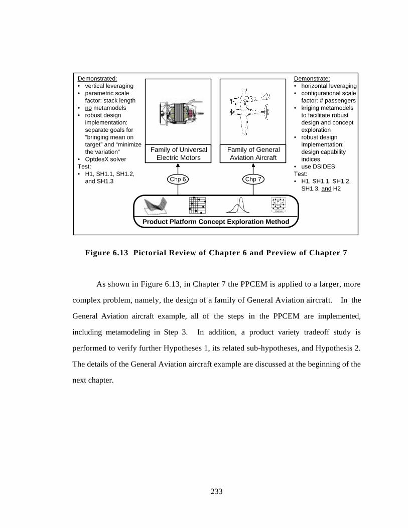
233
Family of General Aviation Aircraft
Platform
Product Platform Concept Exploration Method
Family of UniversalElectric Motors
Chp 7Chp 6
Demonstrated:• vertical leveraging• parametric scale
factor: stack length• no metamodels• robust design
implementation:separate goals for“bringing mean ontarget” and “minimizethe variation”
• OptdesX solverTest:• H1, SH1.1, SH1.2,
and SH1.3
Demonstrate:• horizontal leveraging• configurational scale
factor: # passengers• kriging metamodels
to facilitate robustdesign and concept exploration
• robust designimplementation:design capabilityindices
• use DSIDESTest:• H1, SH1.1, SH1.2,
SH1.3, and H2
Figure 6.13 Pictorial Review of Chapter 6 and Preview of Chapter 7
As shown in Figure 6.13, in Chapter 7 the PPCEM is applied to a larger, more
complex problem, namely, the design of a family of General Aviation aircraft. In the
General Aviation aircraft example, all of the steps in the PPCEM are implemented,
including metamodeling in Step 3. In addition, a product variety tradeoff study is
performed to verify further Hypotheses 1, its related sub-hypotheses, and Hypothesis 2.
The details of the General Aviation aircraft example are discussed at the beginning of the
next chapter.
234
7. CHAPTER 7
DESIGN OF A FAMILY OF GENERALAVIATION AIRCRAFT
In this chapter, the PPCEM is applied in full to the design of a family of General
Aviation aircraft (GAA) for final verification of the method. The layout of this chapter
parallels that of the universal motor case study in the previous chapter. Motivation and
background for the GAA are given in Section 7.1, along with Step 1 of the PPCEM,
namely, creation of an appropriate market segmentation grid for the family of GAA to
accommodate the problem requirements. Based on the desired horizontal leveraging
strategy, the scale factor for the problem is taken as the number of passengers on the
aircraft as explained in Section 7.2; the control factors and responses for the family of GAA
also are described in Section 7.2 as part of Step 2 of the PPCEM. Kriging metamodels
then are created for the mean and standard deviation of each response for the family of
GAA in Section 7.3. After validating the accuracy of the metamodels, a compromise DSP
for the family of aircraft is formulated in Section 7.4 and exercised in Section 7.5 to
develop the GAA platform portfolio. Ramifications of the results and comparison of the
PPCEM solutions against individually designed benchmark aircraft are discussed in Section
7.6. In addition, a product variety tradeoff study is performed, making use of the non-
235
commonality indices (NCI) and performance deviation indices (PDI) to examine the
tradeoff between the two within the family of GAA.
As shown in Table 7.1, all but Hypothesis 3 are verified further in this chapter. As
mentioned in the preceding paragraph, the market segmentation grid is used to identify a
horizontal leveraging strategy for the GAA product family providing further verification of
Sub-Hypothesis 1.1. The use of design capability indices is demonstrated to aggregate the
product family specifications (SH1.3) and facilitate the development of a product platform
which is robust (SH1.2) to variations in the number of passengers on the aircraft, the scale
factor. Furthermore, kriging metamodels are exploited in this chapter to facilitate the
implementation of robust design within the PPCEM, providing further support for
Hypothesis 2. Space filling designs are utilized to create these metamodels; however, only
one type of design is used—an orthogonal array—and Hypothesis 3 is not tested.
Table 7.1 Hypotheses Tested in Chapter 7
Hypothesis Chp 6 Chp 7H1 Product Platform Concept Exploration
Method X XSH1.1 Usefulness of market segmentation
grid X XSH1.2 Robust design of scalable product
platform X XSH1.3 Aggregating product family
specifications X XH2 Utility of kriging for metamodeling
deterministic computer experiments X
A summary of the findings and lessons learned in this example are summarized at
the end of the chapter in Section 7.7. The objective in the summary is to describe how
Hypothesis 1 has been verified further through this example. A brief look ahead to Chapter
8 is given in this last section.

236
7.1 STEP 1: DEVELOPMENT OF THE MARKET SEGMENTATION GRID
Before developing the market segmentation grid, an overview of the General
Aviation aircraft example is given in the next section. This is followed in Section 7.1.2
with a brief overview of the phases of aircraft design. The market segmentation grid for
the General Aviation aircraft example is presented in Section 7.1.3 along with the baseline
design which provides the starting point for designing the family of GAA.
7 .1 .1 Overview of the General Aviation Aircraft Example Problem
What is a General Aviation aircraft? The term General Aviation encompasses all
flights except military operations and commercial carriers. Its potential buyers form a
diverse group that include weekend and recreational pilots, training pilots and instructors,
traveling business executives and even small commercial operators. Satisfying a group
with such diverse needs and economic potential poses a constant challenge for the General
Aviation industry because it is impossible to satisfy all of the market needs with a single
aircraft. The present financial and legal pressures endured by the General Aviation sector
makes small production runs of specialized models unprofitable. As a result, many
General Aviation aircraft are no longer being produced, and the few remaining models are
beyond the financial capability of all but the wealthiest buyers.
In an effort to revitalize the General Aviation sector, the National Aeronautics and
Space Administration (NASA) and the Federal Aviation Administration (FAA) recently
sponsored a General Aviation Design Competition (NASA and FAA, 1994). For this
work, a General Aviation aircraft (GAA) is defined as follows:
• a fixed-wing, single-engine, single-pilot, propeller driven aircraft,
• carries 2-6 passengers,
• cruises at 150-300 kts, and

237
• has a range of 800-1000 nautical miles.
One solution to the GAA crisis is to develop a family of aircraft which can be
adapted easily to satisfy distinct groups of customer demands. Therefore, the purpose in
this example is to develop the following:
a family of aircraft scaled around the two, four, and six seater configurations using
the PPCEM. This family of General Aviation aircraft must be capable of satisfying
the diverse demands of the General Aviation buyers at an affordable price and
operating cost while meeting desired technical and economic considerations.
In order to realize this objective and demonstrate the application of the PPCEM, a brief
overview of aircraft design is given in the next section. This is followed in Section 7.1.3
with the development of the market segmentation grid—Step 1 of the PPCEM—for the
family of GAA.
7 .1 .2 Brief Overview of Aircraft Design
How does one go about designing an aircraft? Aircraft design traditionally is
divided into three phases, namely, conceptual, preliminary, and detailed design as
illustrated in Figure 7.1. If manufacturing design is considered as a part of the design
process, design for production can be added as a fourth phase. The first two phases of
aircraft design, the conceptual and preliminary phases, are sometimes combined and called
advanced design or synthesis in the aerospace industry, while follow-on phases are called
project design or analysis. More detailed descriptions of the decisions made in each phase
and the disciplines involved in aircraft design can be found in, e.g., (Bond and Ricci,
1992). Specifically, the efforts in this example are directed toward utilizing the computer
within the traditional conceptual phase of aircraft design as it is defined in (Nicolai, 1984).
Conceptual Design Phase: In this phase, the general size and configuration of the
aircraft is determined. Parametric trade studies are conducted using preliminary
estimates of aerodynamics and weights to determine the best wing loading, wing
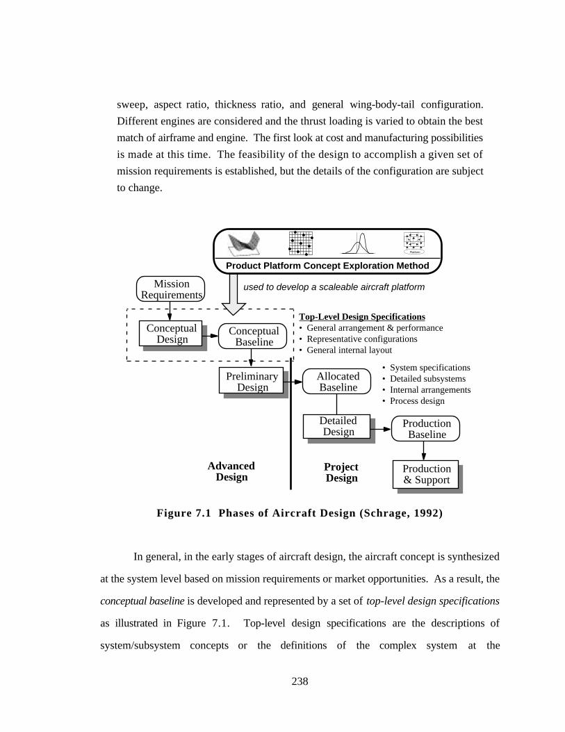
238
sweep, aspect ratio, thickness ratio, and general wing-body-tail configuration.
Different engines are considered and the thrust loading is varied to obtain the best
match of airframe and engine. The first look at cost and manufacturing possibilities
is made at this time. The feasibility of the design to accomplish a given set of
mission requirements is established, but the details of the configuration are subject
to change.
Mission Requirements
Conceptual Baseline
Allocated Baseline
Production Baseline
Top-Level Design Specifications• General arrangement & performance• Representative configurations• General internal layout
• System specifications• Detailed subsystems• Internal arrangements• Process design
AdvancedDesign
ProjectDesign
Production & Support
Preliminary Design
Conceptual Design
Detailed Design
used to develop a scaleable aircraft platform
Platform
Product Platform Concept Exploration Method
Figure 7.1 Phases of Aircraft Design (Schrage, 1992)
In general, in the early stages of aircraft design, the aircraft concept is synthesized
at the system level based on mission requirements or market opportunities. As a result, the
conceptual baseline is developed and represented by a set of top-level design specifications
as illustrated in Figure 7.1. Top-level design specifications are the descriptions of
system/subsystem concepts or the definitions of the complex system at the
239
system/subsystem level. Top-level design specifications are used as the starting point for
the preliminary design at the subsystem level, and form the basis for the specifications
(functional properties) that are developed during the preliminary design phase. These top-
level design specifications include variables such as aspect ratio, thickness ratio, and wing-
body-tail configuration. The top-level design specifications can be continuous (e.g., aspect
ratio = 7-11) or they can be discrete design concepts (e.g., single- or twin-engine, single,
number of propeller blades, high or low wing, and fixed or retractable landing gear). The
settings of the top-level design specifications define the conceptual baseline which becomes
the configuration input for preliminary design, where the system is decomposed for more
sophisticated analysis by discipline, subsystem, or component. The reader is referred to
(Koch, 1997) for more discussion on the resulting “requirements flowdown” process.
Several synthesis and analysis programs have been created to facilitate the
conceptual and preliminary design of aircraft and hence the development of these top-level
design specifications. One such program is entitled FLOPS (FLight OPtimization System
(McCullers, 1993)). FLOPS is a multidisciplinary system of computer programs for
conceptual and preliminary design and evaluation of advanced aircraft concepts. Another
program is called GASP (General Aviation Synthesis Program (NASA, 1978)). GASP is
a computer program which performs tasks specifically associated with the conceptual
design of General Aviation aircraft; consequently, it has been selected as the synthesis
program for use in this example.
What is GASP and how does it work? GASP is a synthesis and analysis computer
program which facilitates parametric studies of small aircraft. GASP specializes in small
fixed-wing aircraft employing propulsion systems varying from a single piston engine with
fixed pitch propeller through a twin turboprop/turbofan powered business or transport type
aircraft. GASP contains an overall control module and six technology submodules which
240
perform the various independent studies required in the design of General Aviation or small
transport type aircraft. The six technology submodules include the following:
• Geometry Module: By inputting parameters such as the number of passengers,
aspect ratio, taper ratio, sweep angles and thicknesses of wing and tail surfaces, the
dimensions of the aircraft components are calculated.
• Aerodynamics Module: Lift and drag coefficients, lift curve slope computation
due to aspect ratio, sweep angle, Mach number, and induced drag are determined.
• Propulsion Module: Reciprocating and rotating combustion engines,
turboprop, turbofan, turbojet are simulated. The results provide engine thrust and
fuel flow at any flight condition using performance data for the specific engine
used.
• Weight and Balance Module: Weight trend coefficients for gross weight,
payload, and aircraft geometry are used to estimate the center of gravity, travel of
the aircraft, fuel tank size, and compartment weight.
• Mission Performance Module: All of the mission segments such as taxi, take
off, climb, cruise and landing are analyzed including the total range. The program
also calculates the best rate of climb, high speed climb, and other characteristics.
• Economics Module: Manufacturing and operating costs are estimated based on
the date of inception of the program (i.e., in 1970's dollars).
Input variables for GASP are general indicators of aircraft type, size, and
performance. The numerical output from GASP includes many aircraft design
characteristics such as range, direct operating cost, maximum cruise speed, and lift-to-drag
ratio. For conceptual design of an aircraft, GASP is used to find appropriate settings for
the top-level design specifications that satisfy the design requirements. By utilizing GASP
as the simulation package within the PPCEM, the PPCEM can be used to develop a set of
top-level design specifications for a suitable aircraft platform which is good for the entire
family of aircraft as shown in Figure 7.1. The first step in the PPCEM is to develop the
market segmentation grid which is accomplished in the next section.
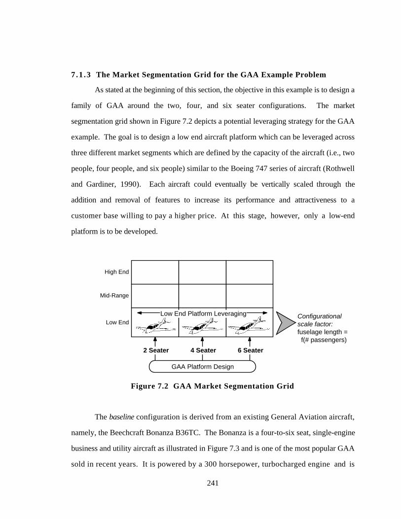
241
7 .1 .3 The Market Segmentation Grid for the GAA Example Problem
As stated at the beginning of this section, the objective in this example is to design a
family of GAA around the two, four, and six seater configurations. The market
segmentation grid shown in Figure 7.2 depicts a potential leveraging strategy for the GAA
example. The goal is to design a low end aircraft platform which can be leveraged across
three different market segments which are defined by the capacity of the aircraft (i.e., two
people, four people, and six people) similar to the Boeing 747 series of aircraft (Rothwell
and Gardiner, 1990). Each aircraft could eventually be vertically scaled through the
addition and removal of features to increase its performance and attractiveness to a
customer base willing to pay a higher price. At this stage, however, only a low-end
platform is to be developed.
Low End
Mid-Range
High End
GAA Platform Design
2 Seater 4 Seater 6 Seater
Configurationalscale factor:fuselage length = f(# passengers)
Low End Platform Leveraging
Figure 7.2 GAA Market Segmentation Grid
The baseline configuration is derived from an existing General Aviation aircraft,
namely, the Beechcraft Bonanza B36TC. The Bonanza is a four-to-six seat, single-engine
business and utility aircraft as illustrated in Figure 7.3 and is one of the most popular GAA
sold in recent years. It is powered by a 300 horsepower, turbocharged engine and is
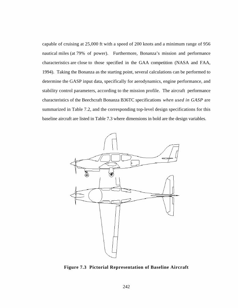
242
capable of cruising at 25,000 ft with a speed of 200 knots and a minimum range of 956
nautical miles (at 79% of power). Furthermore, Bonanza’s mission and performance
characteristics are close to those specified in the GAA competition (NASA and FAA,
1994). Taking the Bonanza as the starting point, several calculations can be performed to
determine the GASP input data, specifically for aerodynamics, engine performance, and
stability control parameters, according to the mission profile. The aircraft performance
characteristics of the Beechcraft Bonanza B36TC specifications when used in GASP are
summarized in Table 7.2, and the corresponding top-level design specifications for this
baseline aircraft are listed in Table 7.3 where dimensions in bold are the design variables.
Figure 7.3 Pictorial Representation of Baseline Aircraft
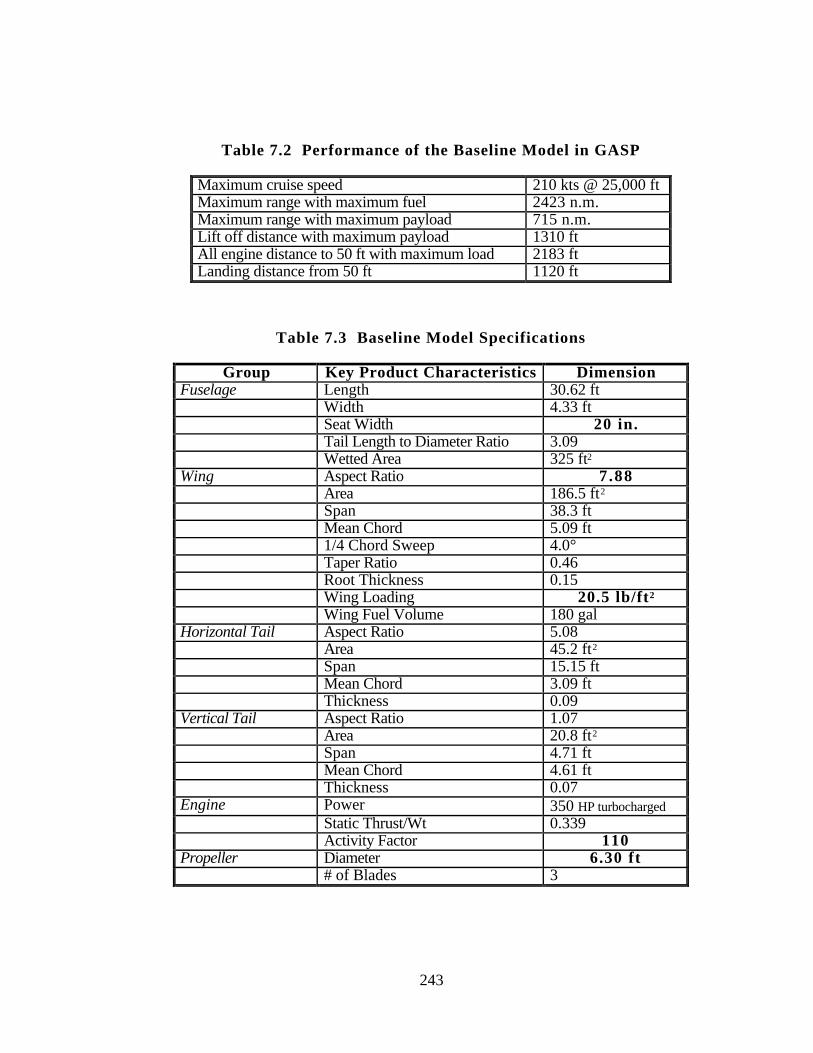
243
Table 7.2 Performance of the Baseline Model in GASP
Maximum cruise speed 210 kts @ 25,000 ftMaximum range with maximum fuel 2423 n.m.Maximum range with maximum payload 715 n.m.Lift off distance with maximum payload 1310 ftAll engine distance to 50 ft with maximum load 2183 ftLanding distance from 50 ft 1120 ft
Table 7.3 Baseline Model Specifications
Group Key Product Characteristics DimensionFuselage Length 30.62 ft
Width 4.33 ftSeat Width 20 in.Tail Length to Diameter Ratio 3.09Wetted Area 325 ft2
Wing Aspect Ratio 7.88Area 186.5 ft2
Span 38.3 ftMean Chord 5.09 ft1/4 Chord Sweep 4.0°Taper Ratio 0.46Root Thickness 0.15Wing Loading 20.5 lb/ft2
Wing Fuel Volume 180 galHorizontal Tail Aspect Ratio 5.08
Area 45.2 ft2
Span 15.15 ftMean Chord 3.09 ftThickness 0.09
Vertical Tail Aspect Ratio 1.07Area 20.8 ft2
Span 4.71 ftMean Chord 4.61 ftThickness 0.07
Engine Power 350 HP turbochargedStatic Thrust/Wt 0.339Activity Factor 110
Propeller Diameter 6.30 ft# of Blades 3
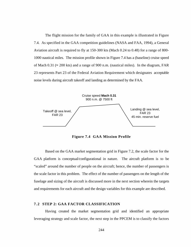
244
The flight mission for the family of GAA in this example is illustrated in Figure
7.4. As specified in the GAA competition guidelines (NASA and FAA, 1994), a General
Aviation aircraft is required to fly at 150-300 kts (Mach 0.24 to 0.48) for a range of 800-
1000 nautical miles. The mission profile shown in Figure 7.4 has a (baseline) cruise speed
of Mach 0.31 (≈ 200 kts) and a range of 900 n.m. (nautical miles). In the diagram, FAR
23 represents Part 23 of the Federal Aviation Requirement which designates acceptable
noise levels during aircraft takeoff and landing as determined by the FAA.
Takeoff @ sea level,FAR 23
Cruise speed Mach 0.31900 n.m. @ 7500 ft
Landing @ sea level,FAR 23
45 min. reserve fuel
Figure 7.4 GAA Mission Profile
Based on the GAA market segmentation grid in Figure 7.2, the scale factor for the
GAA platform is conceptual/configurational in nature. The aircraft platform is to be
“scaled” around the number of people on the aircraft; hence, the number of passengers is
the scale factor in this problem. The effect of the number of passengers on the length of the
fuselage and sizing of the aircraft is discussed more in the next section wherein the targets
and requirements for each aircraft and the design variables for this example are described.
7.2 STEP 2: GAA FACTOR CLASSIFICATION
Having created the market segmentation grid and identified an appropriate
leveraging strategy and scale factor, the next step in the PPCEM is to classify the factors

245
within the GAA problem. The general configuration of each aircraft has been fixed at three
propeller blades, high wing position, and retractable landing gear based on previous work
(Simpson, 1995). The design variables (i.e., control factors) and corresponding ranges of
interest in this study are as follows:
1. Cruise speed, CSPD ∈ [Mach 0.24, Mach 0.48]; baseline is Mach 0.31
2. Aspect ratio, AR ∈ [7, 11]; baseline is 7.88
3. Propeller diameter, DPRP ∈ [5.0 ft, 5.96 ft]; baseline is 6.3 ft
4. Wing loading, WL ∈ [19.0 lb/ft2, 25.0 lb/ft2]; baseline is 20.5
5. Engine activity factor, AF ∈ [85, 110]; baseline is 100
6. Seat width, WS ∈ [14.0 in, 20.0 in]; baseline is 20 in.
A brief description of the importance and effects of each of these variables is included in
Section F.1.
There are a total of nine responses (i.e., requirements and goals) which are of
interest for each aircraft: takeoff noise, direct operating cost, ride roughness, empty weight
and fuel weight, purchase price, and maximum cruise speed, flight range and lift/drag ratio.
In general, it is desired to find settings of the design variables which:
• lower direct operating cost, purchase price, empty weight and fuel weight to their
targets;
• raise maximum cruise speed, flight range, and lift/drag ratio to their targets; and
• meet constraints on the maximum takeoff noise, ride roughness, direct operating
cost, empty weight, and fuel weight, and minimum flight range.
The constraint values and target values for the goals employed in this example are listed in
Table 7.4 and Table 7.5, respectively. As such, these constraints and targets define each
market niche for each of the three aircraft. As shown in Table 7.4 the constraint values for
take-off noise, direct operating cost, ride roughness aircraft empty weight, and range are
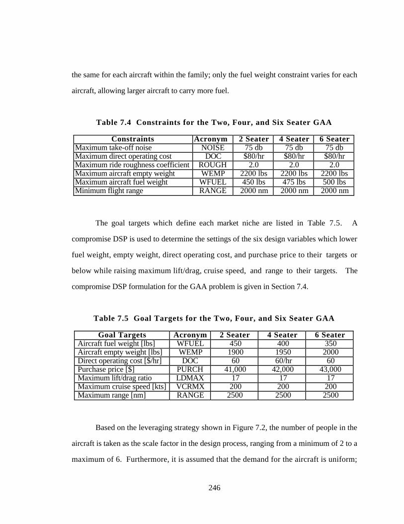
246
the same for each aircraft within the family; only the fuel weight constraint varies for each
aircraft, allowing larger aircraft to carry more fuel.
Table 7.4 Constraints for the Two, Four, and Six Seater GAA
Constraints Acronym 2 Seater 4 Seater 6 SeaterMaximum take-off noise NOISE 75 db 75 db 75 dbMaximum direct operating cost DOC $80/hr $80/hr $80/hrMaximum ride roughness coefficient ROUGH 2.0 2.0 2.0Maximum aircraft empty weight WEMP 2200 lbs 2200 lbs 2200 lbsMaximum aircraft fuel weight WFUEL 450 lbs 475 lbs 500 lbsMinimum flight range RANGE 2000 nm 2000 nm 2000 nm
The goal targets which define each market niche are listed in Table 7.5. A
compromise DSP is used to determine the settings of the six design variables which lower
fuel weight, empty weight, direct operating cost, and purchase price to their targets or
below while raising maximum lift/drag, cruise speed, and range to their targets. The
compromise DSP formulation for the GAA problem is given in Section 7.4.
Table 7.5 Goal Targets for the Two, Four, and Six Seater GAA
Goal Targets Acronym 2 Seater 4 Seater 6 SeaterAircraft fuel weight [lbs] WFUEL 450 400 350Aircraft empty weight [lbs] WEMP 1900 1950 2000Direct operating cost [$/hr] DOC 60 60/hr 60Purchase price [$] PURCH 41,000 42,000 43,000Maximum lift/drag ratio LDMAX 17 17 17Maximum cruise speed [kts] VCRMX 200 200 200Maximum range [nm] RANGE 2500 2500 2500
Based on the leveraging strategy shown in Figure 7.2, the number of people in the
aircraft is taken as the scale factor in the design process, ranging from a minimum of 2 to a
maximum of 6. Furthermore, it is assumed that the demand for the aircraft is uniform;
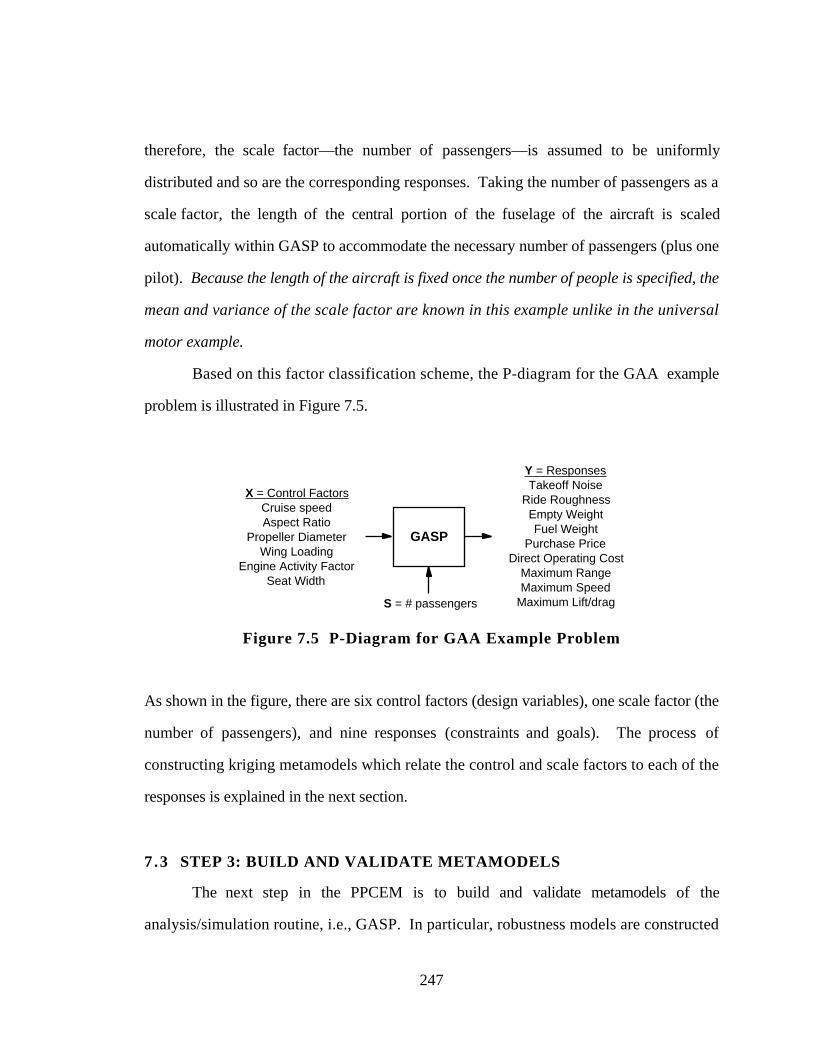
247
therefore, the scale factor—the number of passengers—is assumed to be uniformly
distributed and so are the corresponding responses. Taking the number of passengers as a
scale factor, the length of the central portion of the fuselage of the aircraft is scaled
automatically within GASP to accommodate the necessary number of passengers (plus one
pilot). Because the length of the aircraft is fixed once the number of people is specified, the
mean and variance of the scale factor are known in this example unlike in the universal
motor example.
Based on this factor classification scheme, the P-diagram for the GAA example
problem is illustrated in Figure 7.5.
X = Control FactorsCruise speedAspect Ratio
Propeller DiameterWing Loading
Engine Activity FactorSeat Width
Y = ResponsesTakeoff Noise
Ride RoughnessEmpty WeightFuel Weight
Purchase PriceDirect Operating Cost
Maximum RangeMaximum Speed
Maximum Lift/dragS = # passengers
GASP
Figure 7.5 P-Diagram for GAA Example Problem
As shown in the figure, there are six control factors (design variables), one scale factor (the
number of passengers), and nine responses (constraints and goals). The process of
constructing kriging metamodels which relate the control and scale factors to each of the
responses is explained in the next section.
7.3 STEP 3: BUILD AND VALIDATE METAMODELS
The next step in the PPCEM is to build and validate metamodels of the
analysis/simulation routine, i.e., GASP. In particular, robustness models are constructed
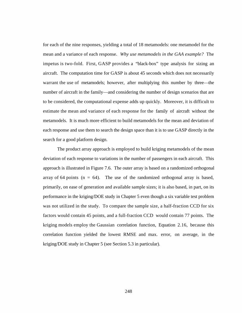
248
for each of the nine responses, yielding a total of 18 metamodels: one metamodel for the
mean and a variance of each response. Why use metamodels in the GAA example? The
impetus is two-fold. First, GASP provides a “black-box” type analysis for sizing an
aircraft. The computation time for GASP is about 45 seconds which does not necessarily
warrant the use of metamodels; however, after multiplying this number by three—the
number of aircraft in the family—and considering the number of design scenarios that are
to be considered, the computational expense adds up quickly. Moreover, it is difficult to
estimate the mean and variance of each response for the family of aircraft without the
metamodels. It is much more efficient to build metamodels for the mean and deviation of
each response and use them to search the design space than it is to use GASP directly in the
search for a good platform design.
The product array approach is employed to build kriging metamodels of the mean
deviation of each response to variations in the number of passengers in each aircraft. This
approach is illustrated in Figure 7.6. The outer array is based on a randomized orthogonal
array of 64 points (n = 64). The use of the randomized orthogonal array is based,
primarily, on ease of generation and available sample sizes; it is also based, in part, on its
performance in the kriging/DOE study in Chapter 5 even though a six variable test problem
was not utilized in the study. To compare the sample size, a half-fraction CCD for six
factors would contain 45 points, and a full-fraction CCD would contain 77 points. The
kriging models employ the Gaussian correlation function, Equation 2.16, because this
correlation function yielded the lowest RMSE and max. error, on average, in the
kriging/DOE study in Chapter 5 (see Section 5.3 in particular).
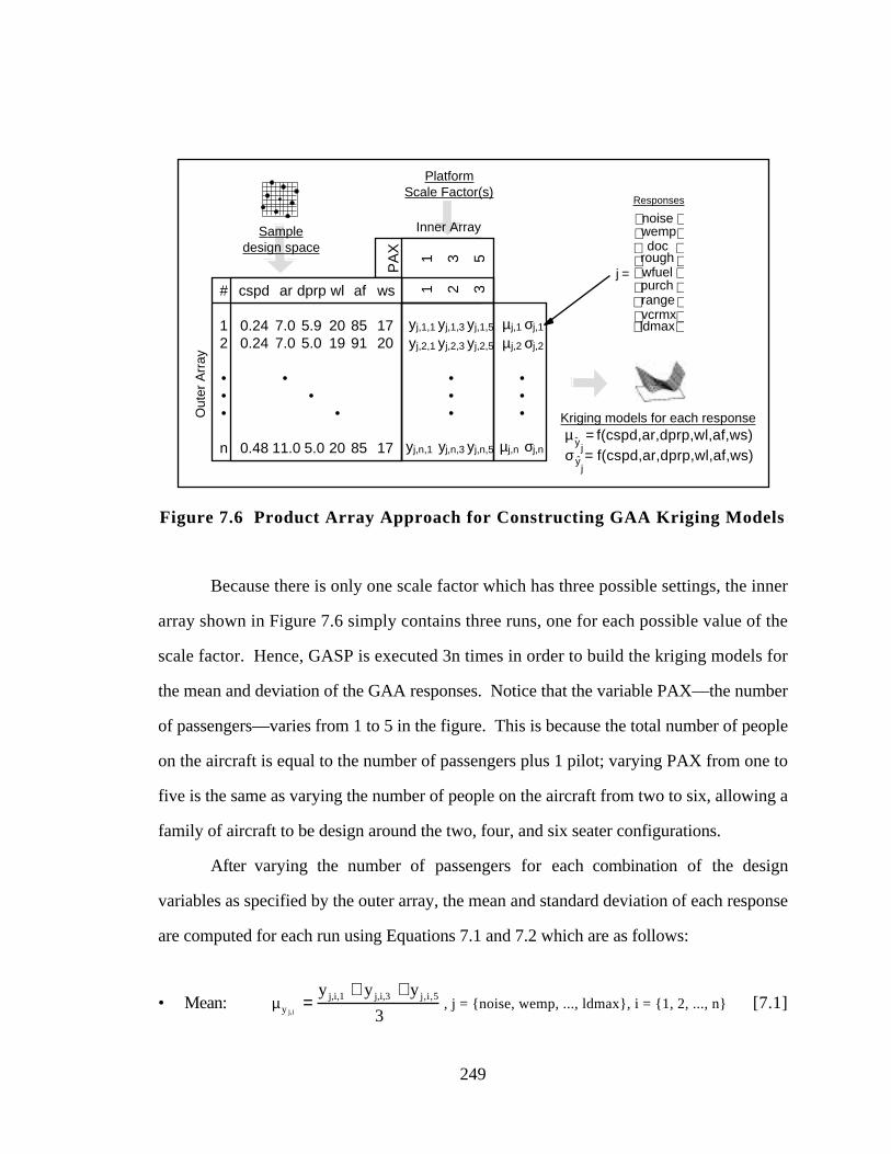
249
Sampledesign space
#P
AX
11
23
35
# cspd ar dprp wl af ws
1 0.24 7.0 5.9 20 85 172 0.24 7.0 5.0 19 91 20
• •• •• •
n 0.48 11.0 5.0 20 85 17
µj,1 σj,1
µj,2 σj,2
• • •
µj,n σj,n
Inner Array
Out
er A
rray
yj,1,1 yj,1,3 yj,1,5
yj,2,1 yj,2,3 yj,2,5
•••
yj,n,1 yj,n,3 yj,n,5µ ˆ y = f(cspd,ar,dprp,wl,af,ws)σ ˆ y = f(cspd,ar,dprp,wl,af,ws)
Responses
j =
noisewempdoc
roughwfuelpurchrangevcrmxldmax
Kriging models for each response
j
j
PlatformScale Factor(s)
Figure 7.6 Product Array Approach for Constructing GAA Kriging Models
Because there is only one scale factor which has three possible settings, the inner
array shown in Figure 7.6 simply contains three runs, one for each possible value of the
scale factor. Hence, GASP is executed 3n times in order to build the kriging models for
the mean and deviation of the GAA responses. Notice that the variable PAX—the number
of passengers—varies from 1 to 5 in the figure. This is because the total number of people
on the aircraft is equal to the number of passengers plus 1 pilot; varying PAX from one to
five is the same as varying the number of people on the aircraft from two to six, allowing a
family of aircraft to be design around the two, four, and six seater configurations.
After varying the number of passengers for each combination of the design
variables as specified by the outer array, the mean and standard deviation of each response
are computed for each run using Equations 7.1 and 7.2 which are as follows:
• Mean: µy j,i=
y j,i,1 + y j,i,3 + y j,i,5
3, j = {noise, wemp, ..., ldmax}, i = {1, 2, ..., n} [7.1]
250
• Std. Dev.: σy j,i=
y j,i,1 − y j,i,5
12, j = {noise, wemp, ..., ldmax}, i = {1, 2, ..., n} [7.2]
Computation of the standard deviation assumes a uniform distribution of the response
because the number of passengers is assumed to vary uniformly over the design space. As
an example, the mean and standard deviation of the direct operating cost, DOC, for the 3rd
experimental design is estimated as follows:
µy DOC,3=
yDOC,3,1 + yDOC,3,3 + yDOC,3,5
3[7.3]
σyDOC,3=
yDOC,3,1 − yDOC,3,5
12[7.4]
It is in this manner that the means and deviations for each response for each experimental
run in the outer array are computed for a given experimental design. Kriging metamodels
then are constructed for the mean and deviation of each response, resulting in 18
metamodels. The kriging algorithm described in Section A.2.1 is used to fit the model; the
fitted values (MLE estimates) for the “best” kriging model for each response are listed in
Section F.2.
A set of 1000 validation points from a random Latin hypercube are used to assess
the accuracy of the GAA kriging models. The maximum error and root mean square error
(RMSE) based on the set of validation points for the kriging models based on the 64 point
orthogonal array are summarized in Table 7.6; both raw values and percentages (of the
sample range) are listed.
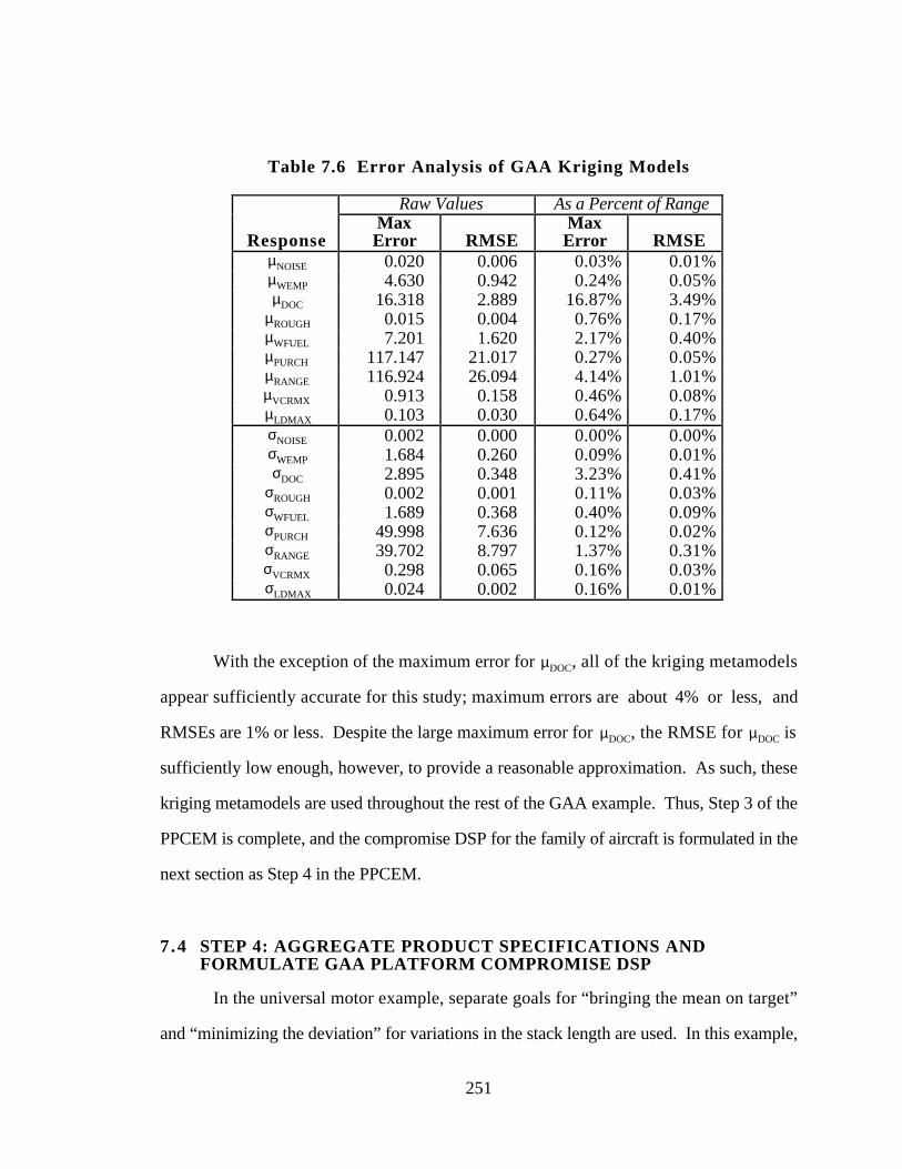
251
Table 7.6 Error Analysis of GAA Kriging Models
Raw Values As a Percent of Range
ResponseMaxError RMSE
MaxError RMSE
µNOISE 0.020 0.006 0.03% 0.01%µWEMP 4.630 0.942 0.24% 0.05%µDOC 16.318 2.889 16.87% 3.49%
µROUGH 0.015 0.004 0.76% 0.17%µWFUEL 7.201 1.620 2.17% 0.40%µPURCH 117.147 21.017 0.27% 0.05%µRANGE 116.924 26.094 4.14% 1.01%µVCRMX 0.913 0.158 0.46% 0.08%µLDMAX 0.103 0.030 0.64% 0.17%σNOISE 0.002 0.000 0.00% 0.00%σWEMP 1.684 0.260 0.09% 0.01%σDOC 2.895 0.348 3.23% 0.41%
σROUGH 0.002 0.001 0.11% 0.03%σWFUEL 1.689 0.368 0.40% 0.09%σPURCH 49.998 7.636 0.12% 0.02%σRANGE 39.702 8.797 1.37% 0.31%σVCRMX 0.298 0.065 0.16% 0.03%σLDMAX 0.024 0.002 0.16% 0.01%
With the exception of the maximum error for µDOC, all of the kriging metamodels
appear sufficiently accurate for this study; maximum errors are about 4% or less, and
RMSEs are 1% or less. Despite the large maximum error for µDOC, the RMSE for µDOC is
sufficiently low enough, however, to provide a reasonable approximation. As such, these
kriging metamodels are used throughout the rest of the GAA example. Thus, Step 3 of the
PPCEM is complete, and the compromise DSP for the family of aircraft is formulated in the
next section as Step 4 in the PPCEM.
7.4 STEP 4: AGGREGATE PRODUCT SPECIFICATIONS ANDFORMULATE GAA PLATFORM COMPROMISE DSP
In the universal motor example, separate goals for “bringing the mean on target”
and “minimizing the deviation” for variations in the stack length are used. In this example,
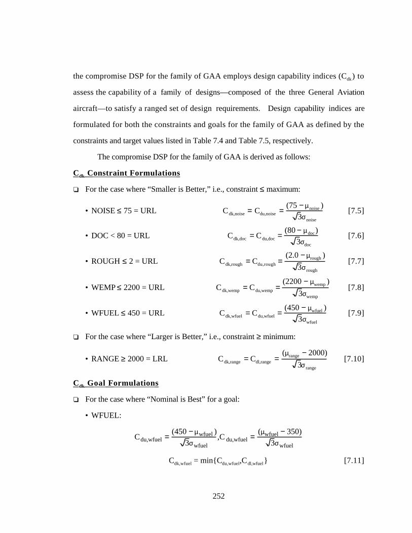
252
the compromise DSP for the family of GAA employs design capability indices (Cdk) to
assess the capability of a family of designs—composed of the three General Aviation
aircraft—to satisfy a ranged set of design requirements. Design capability indices are
formulated for both the constraints and goals for the family of GAA as defined by the
constraints and target values listed in Table 7.4 and Table 7.5, respectively.
The compromise DSP for the family of GAA is derived as follows:
C dk Constraint Formulations
❏ For the case where “Smaller is Better,” i.e., constraint ≤ maximum:
• NOISE ≤ 75 = URL Cdk,noise = Cdu,noise =(75 − µnoise )
3σnoise
[7.5]
• DOC < 80 = URL Cdk,doc = Cdu,doc =(80 − µdoc)
3σdoc
[7.6]
• ROUGH ≤ 2 = URL Cdk,rough = Cdu,rough =(2.0 − µrough )
3σ rough
[7.7]
• WEMP ≤ 2200 = URL Cdk,wemp = Cdu,wemp =(2200 − µwemp )
3σwemp
[7.8]
• WFUEL ≤ 450 = URL Cdk,wfuel = Cdu,wfuel =(450 − µwfuel )
3σwfuel
[7.9]
❏ For the case where “Larger is Better,” i.e., constraint ≥ minimum:
• RANGE ≥ 2000 = LRL Cdk,range = Cdl,range =(µrange − 2000)
3σ range
[7.10]
C dk Goal Formulations
❏ For the case where “Nominal is Best” for a goal:
• WFUEL:
Cdu,wfuel =(450 − µwfuel )
3σwfuel,C du,wfuel =
(µwfuel − 350)
3σwfuel
Cdk,wfuel = min{Cdu,wfuel,Cdl,wfuel} [7.11]
253
• WEMP:
Cdu,wemp =(2000 − µwemp)
3σwemp,Cdu,wemp =
(µwemp − 1900)
3σwemp
Cdk,wemp = min{Cdu,wemp,Cdl,wemp} [7.12]
• PURCH:
Cdu,purch =(43000 − µpurch )
3σpurch,Cdu,purch =
(µpurch − 41000)
3σpurch
Cdk,wfuel = min{Cdu,purch,Cdl,purch} [7.13]
❏ For goals where “Smaller is Better”:
• DOC: Cdk,doc = Cdu,doc =(60 − µdoc )
3σdoc
[7.14]
❏ For the case where “Larger is Better” for a goal:
• LDMAX: Cdk,ldmax = Cdl,ldmax =(µ ldmax −17)
3σ ldmax
[7.15]
• VCRMX: Cdk,vcrmx = Cdl,vcrmx =(µvcrmx − 200)
3σvcrmx
[7.16]
• RANGE: Cdk,range = Cdl,range =(µrange − 2500)
3σ range
[7.17]
The resulting compromise DSP for the GAA product platform using these Cdk
formulations is given in Figure 7.7. There are six design variables, six constraints, and
seven goals. Of the seven goals, three are related to the economic performance of the
aircraft—empty weight (WEMP), purchase price (PURCH), and direct operating cost
(DOC)—and the remaining four are related to the technical performance of the aircraft: fuel
weight (WFUEL), maximum lift/drag (LDMAX), maximum cruise speed (VCRMX), and
maximum flight range (RANGE).
254
Given:❏ Baseline aircraft configuration and mission profile❏ Configuration scale factor = # passengers (where total # seats = # passengers + 1 pilot)❏ Kriging models for mean and standard deviation of each response
Find:❏ The system variables, x:
• cruise speed, CSPD • wing loading, WL• wing aspect ratio, AR • engine activity factor, AF• propeller diameter, DPRP • seat width, WS
❏ The values of the deviation variables associated with G(x):• fuel weight Cdk , d1
-, d1+ • maximum lift/drag Cdk , d5
-, d5+
• empty weight Cdk , d2-, d2
+ • maximum speed Cdk , d6-, d6
+
• direct operating cost Cdk , d3-, d3
+ • maximum range Cdk , d7-, d7
+
• purchase price Cdk , d4-, d4
+
Satisfy:❏ The system constraints, C(x), based on kriging models:
• NOISE Cdk greater than 1: Cdk,noise(x) ≥ 1 [7.5]• DOC Cdk greater than 1: Cdk,doc(x) ≥ 1 [7.6]• ROUGH Cdk greater than 1: Cdk,rough(x) ≥ 1 [7.7]• WEMP Cdk greater than 1: Cdk,wemp(x) ≥ 1 [7.8]• WFUEL Cdk greater than 1: Cdk,wfuel(x) ≥ 1 [7.9]• RANGE Cdk greater than 1: Cdk,range(x) ≥ 1 [7.10]
❏ The system goals, G(x), based on kriging models:• WFUEL Cdk greater than 1: Cdk,noise(x) + d1
- - d1+ = 1.0 [7.11]
• WEMP Cdk greater than 1: Cdk,wemp(x) + d2- - d2
+ = 1.0 [7.12]• DOC Cdk greater than 1: Cdk,doc(x) + d3
- - d3+ = 1.0 [7.13]
• PURCH Cdk greater than 1: Cdk,purch(x) + d4- - d4
+ = 1.0 [7.14]• LDMAX Cdk greater than 1: Cdk,ldmax(x) + d5
- - d5+ = 1.0 [7.15]
• VCRMX Cdk greater than 1: Cdk,vcrmx(x) + d6- - d6
+ = 1.0 [7.16]• RANGE Cdk greater than 1: Cdk,range(x) + d7
- - d7+ = 1.0 [7.17]
❏ Constraints on deviation variables: di- • di
+ = 0 and di-, d i
+ ≥ 0.
❏ The bounds on the system variables:0.24 M ≤ CSPD ≤ 0.48 M 19 lb/ft2 ≤ WL ≤ 25 lb/ft2
7 ≤ AR ≤ 11 85 ≤ AF ≤ 1105.0 ft ≤ DPRP ≤ 5.96 ft 14.0 in ≤ WS ≤ 20.0 in
Minimize:❏ The sum of the deviation variables associated with:
• fuel weight Cdk , d1- • maximum lift/drag Cdk , d5
-
• empty weight Cdk , d2- • maximum speed Cdk , d6
-
• direct operating cost Cdk , d3- • maximum range Cdk , d7
-
• purchase price Cdk , d4-
Z = { f1(d1-), f2(d2
-), f3(d3-), f4(d4
-), f5(d5-), f6(d6
-), f7(d7-) }
Figure 7.7 GAA Product Platform Compromise DSP Formulation
255
Based on this GAA compromise DSP, the initial baseline design is infeasible in two
regards. First, the propeller diameter is too great as explained in Section 7.1 At 6.3 ft, the
speed of the propeller tip is above sonic speed, violating a tipspeed constraint which is not
explicitly modeled in the GAA compromise DSP; thus, the range for the propeller diameter
is set at 5-5.96 ft so that this constraint is always met. Second, the DOC violates the
$80/hr constraint which has been selected. The baseline design still represents a good
design; however, the GAA compromise DSP is being used to improve it as discussed in the
next section wherein the product platform portfolio is developed in Step 5 of the PPCEM.
7.5 STEP 5: DEVELOP THE GAA PLATFORM PORTFOLIO
In order to develop the GAA platform portfolio for the family of GAA to meet the
constraints and goals set forth in Section 7.2, three design scenarios are investigated (see
Table 7.7).
Overall Tradeoff Study: All of the goals are weighted equally in an effort to
develop a platform that simultaneously meets both economic and performance
requirements as best as possible.
Economic Tradeoff Study: Economic related goals (Cdk’s for empty weight,
purchase price, and direct operating cost) are given top priority to find a platform
which meets all of the economic requirements as best as possible; satisfying
performance goals is second priority.
Performance Tradeoff Study: Performance related goals (Cdk’s for fuel weight,
max. lift/drag, max. speed, and max. range) are placed at the first priority level to
develop a platform that satisfies all of the performance requirements as best as
possible; meanwhile, economic goals are given second priority.
The corresponding deviation function formulations for each scenario are listed in Table 7.7.
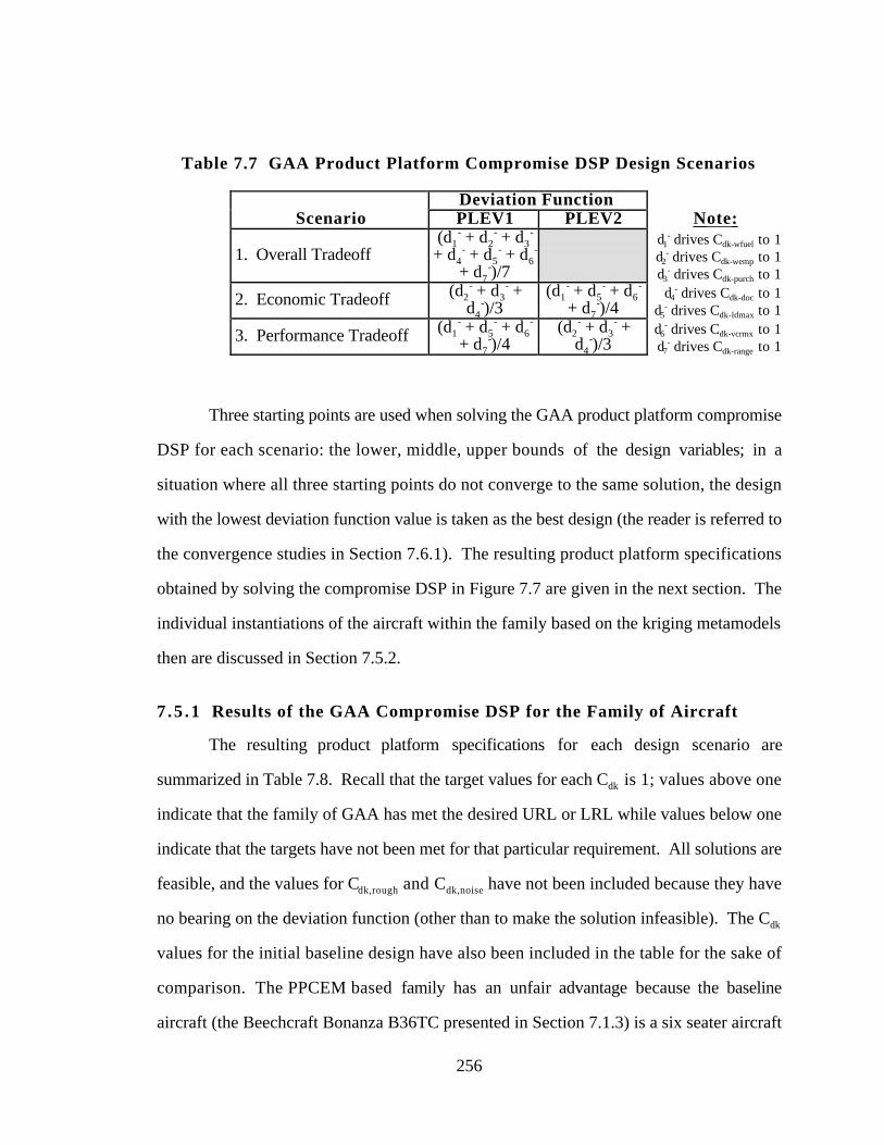
256
Table 7.7 GAA Product Platform Compromise DSP Design Scenarios
Deviation FunctionScenario PLEV1 PLEV2 Note:
1. Overall Tradeoff(d1
- + d2- + d3
-
+ d4- + d5
- + d6-
+ d7-)/7
d1- drives Cdk-wfuel to 1
d2- drives Cdk-wemp to 1
d3- drives Cdk-purch to 1
2. Economic Tradeoff (d2- + d3
- +d4
-)/3(d1
- + d5- + d6
-
+ d7-)/4
d4- drives Cdk-doc to 1
d5- drives Cdk-ldmax to 1
3. Performance Tradeoff (d1- + d5
- + d6-
+ d7-)/4
(d2- + d3
- +d4
-)/3d6
- drives Cdk-vcrmx to 1d7
- drives Cdk-range to 1
Three starting points are used when solving the GAA product platform compromise
DSP for each scenario: the lower, middle, upper bounds of the design variables; in a
situation where all three starting points do not converge to the same solution, the design
with the lowest deviation function value is taken as the best design (the reader is referred to
the convergence studies in Section 7.6.1). The resulting product platform specifications
obtained by solving the compromise DSP in Figure 7.7 are given in the next section. The
individual instantiations of the aircraft within the family based on the kriging metamodels
then are discussed in Section 7.5.2.
7 .5 .1 Results of the GAA Compromise DSP for the Family of Aircraft
The resulting product platform specifications for each design scenario are
summarized in Table 7.8. Recall that the target values for each Cdk is 1; values above one
indicate that the family of GAA has met the desired URL or LRL while values below one
indicate that the targets have not been met for that particular requirement. All solutions are
feasible, and the values for Cdk,rough and Cdk,noise have not been included because they have
no bearing on the deviation function (other than to make the solution infeasible). The Cdk
values for the initial baseline design have also been included in the table for the sake of
comparison. The PPCEM based family has an unfair advantage because the baseline
aircraft (the Beechcraft Bonanza B36TC presented in Section 7.1.3) is a six seater aircraft
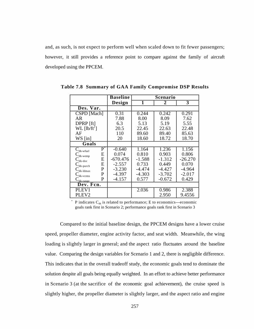
257
and, as such, is not expect to perform well when scaled down to fit fewer passengers;
however, it still provides a reference point to compare against the family of aircraft
developed using the PPCEM.
Table 7.8 Summary of GAA Family Compromise DSP Results
Baseline ScenarioDesign 1 2 3
Des. Var.CSPD [Mach] 0.31 0.244 0.242 0.291AR 7.88 8.00 8.09 7.62DPRP [ft] 6.3 5.13 5.19 5.55WL [lb/ft2] 20.5 22.45 22.63 22.48AF 110 89.60 89.40 85.63WS [in] 20 18.60 18.72 18.70
GoalsCdk-wfuel P* -0.640 1.164 1.236 1.156Cdk-wemp E 0.074 0.810 0.903 0.806Cdk-doc E -670.476 -1.588 -1.312 -26.270Cdk-purch E -2.557 0.733 0.449 0.070Cdk-ldmax P -3.230 -4.474 -4.427 -4.964Cdk-vcrmx P -4.397 -4.303 -3.702 -2.017Cdk-range P -4.157 0.577 -0.672 0.429Dev. Fcn.
PLEV1 2.036 0.986 2.388PLEV2 2.950 9.4556
* P indicates Cdk is related to performance; E to economics—economicgoals rank first in Scenario 2; performance goals rank first in Scenario 3
Compared to the initial baseline design, the PPCEM designs have a lower cruise
speed, propeller diameter, engine activity factor, and seat width. Meanwhile, the wing
loading is slightly larger in general; and the aspect ratio fluctuates around the baseline
value. Comparing the design variables for Scenario 1 and 2, there is negligible difference.
This indicates that in the overall tradeoff study, the economic goals tend to dominate the
solution despite all goals being equally weighted. In an effort to achieve better performance
in Scenario 3 (at the sacrifice of the economic goal achievement), the cruise speed is
slightly higher, the propeller diameter is slightly larger, and the aspect ratio and engine
258
activity factor are slightly lower for this scenario than either Scenario 1 or 2. Thus, in
order to maintain sufficient flexibility to achieve all the design considerations in all three
scenarios, the resulting product platform is taken as follows:
• Cruise speed = Mach 0.242 or Mach 0.291 (if performance is first priority)
• Aspect ratio = 7.85 ± 0.24
• Propeller diameter = 5.34 ± 0.2 ft
• Wing loading = 22.54 ± 0.09 lb/ft2
• Engine activity factor = 87.61 ± 2.0
• Seat width = 18.66 ± 0.06 in
These values comprise the range of values that cruise speed, aspect ratio, etc. should be
allowed to take in order to meet the goals as best as possible in any of the three design
scenarios. It is these values which define the GAA product platform around which the
family of aircraft are created.
Before instantiating the individual aircraft to examine how well they perform given
these specifications, notice in Table 7.8 that very few Cdk goals achieve their target of 1;
only Cdk,wfuel is consistently larger than 1, indicating that the family of GAA are capable of
meeting the specified fuel weight targets. The empty weight Cdk and purchase price Cdk are
the second best with Cdk,range performing well in Scenarios 1 and 3. All Cdk values are
improved over the baseline design except for Cdk,ldmax which has decreased slightly. In
Scenario 2, the economic Cdk’s for direct operating cost and empty weight improve slightly
but at the expense of a slight decrease in the purchase price Cdk when compared to the value
obtained in Scenario 1. The big tradeoff between the economic and performance goals in
Scenarios 2 and 3 is best seen in Cdk,doc. In all three scenarios, the family of GAA is far
from achieving its target of $60/hr for the direct operating cost as indicated by the low
values for Cdk,doc; however, in Scenario 3 when achieving performance goals is given a
259
higher priority than economic goals, Cdk,doc is even worse, indicating the compromise
between a family of aircraft that has performs well versus one that is economical.
To study these compromises further, five more design scenarios are formulated (see
Section F.4) to determine whether it is the Cdk formulation that is performing poorly or that
the targets are difficult to achieve. The results are listed separately in Section F.4 and
discussed therein. The end result of examining all these design scenarios is learning that
significant tradeoffs are occurring in Scenarios 1, 2, and 3 where the economic and
performance Cdk goals are equally weighted at different priority levels. Only when a
particular Cdk is given first priority (i.e., placed at PLEV1) in the GAA product platform
compromise DSP can the target (Cdk ≥ 1) be achieved. Any other time, the solutions from
the GAA product platform compromise DSP represent the best possible compromise which
can be obtained for a particular design scenario, poor Cdk value or not. Furthermore, the
deviation function values shown in Table 7.8 are not much value in and of themselves
because they are based on how well the Cdk achieve their target of 1. Recall that Cdk is only
a means to end, i.e., to generate a family of aircraft which satisfies the given ranged set of
requirements as well as possible . What is important, however, is the resulting aircraft
which come from instantiating the PPCEM aircraft platform to accommodate two, four, and
six passengers.
7 .5 .2 Instantiation of the Family of General Aviation Aircraft
Unlike in the universal motor example, instantiation of the individual aircraft within
the GAA product family only requires specifying the number of passengers on the plane,
not solving another compromise DSP to find the best stack length to meet a particular
torque requirement. The individual constraints and goals for each aircraft must be
formulated first, however, based on the specifications given in Section 7.2. Based on the
260
requirements in Table 7.4, the individual constraints for each aircraft are given by the
following:
• noise [dbA]: NOISE(x) ≤ 75 dbA [7.18]
• direct operating cost [$/hr]: DOC(x) ≤ $80/hr [7.19]
• ride roughness: ROUGH(x) ≤ 2.0 [7.20]
• aircraft empty weight [lbs]: WEMP(x) ≤ 2200 lbs [7.21]
• aircraft fuel weight [lbs]: WFUEL(x) ≤ Ci,wfuel [7.22]
• maximum flight range [nm]: RANGE(x) ≥ 2200 nm [7.23]
where Ci,wfuel = {450 lbs, 475 lbs, 500 lbs} and i = {1, 3, 5} passengers. Meanwhile, the
individual goals based on the targets in Table 7.5 for each aircraft are given by:
• aircraft fuel weight [lbs]: WFUEL(x)/Ti,wfuel + d1- - d1
+ = 1.0 [7.24]
• aircraft empty weight [lbs]: WEMP(x)/Ti,wemp + d2- - d2
+ = 1.0 [7.25]
• direct operating cost [$/hr]: DOC(x)/60 + d3- - d3
+ = 1.0 [7.26]
• purchase price [$]: PURCH(x)/Ti,purch + d4- - d4
+ = 1.0 [7.27]
• maximum lift/drag: LDMAX(x)/17 + d5- - d5
+ = 1.0 [7.28]
• maximum cruise speed [kts]: VCRMX(x)/200 + d6- - d6
+ = 1.0 [7.29]
• maximum range [nm]: RANGE(x)/2500 + d7- - d7
+ = 1.0 [7.30]
where Ti,wfuel = {450 lbs, 400 lbs, 350 lbs}, Ti,wemp = {1900 lbs, 1950 lbs, 2000 lbs},
Ti,purch = {$41000, $42000, $43000} and i = {1, 3, 5} passengers. Based on these goals,
the deviation function for each aircraft is a combination of: d1+, d2
+, d3+, d4
+, d5-, d6
-, and d7-
because it is desired to lower fuel weight, empty weight, direct operating cost, and
purchase price to their targets and to raise maximum lift/drag, cruise speed, and range to
theirs. The resulting deviation function formulations for each aircraft for each scenario is
listed in Table 7.9. These deviation functions are identical to those listed in Table 7.7
except that di+ and di
- are for the individual goals of each aircraft and not the Cdk for the
family (which only uses di- to raise Cdk to its target of 1 as noted in Table 7.7).
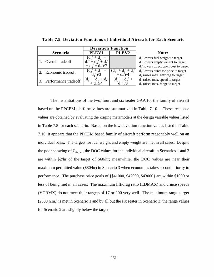
261
Table 7.9 Deviation Functions of Individual Aircraft for Each Scenario
Deviation FunctionScenario PLEV1 PLEV2 Note:
1. Overall tradeoff(d1
+ + d2+ +
d3+ + d4
+ + d5-
+ d6- + d7
-)/7
d1+ lowers fuel weight to target
d2+ lowers empty weight to target
d3+ lowers direct oper. cost to target
2. Economic tradeoff (d2+ + d3
+ +d4
+)/3(d1
+ + d5- + d6
-
+ d7-)/4
d4+ lowers purchase price to target
d5- raises max. lift/drag to target
3. Performance tradeoff (d1+ + d5
- + d6-
+ d7-)/4
(d2+ + d3
+ +d4
+)/3d6
- raises max. speed to targetd7
- raises max. range to target
The instantiations of the two, four, and six seater GAA for the family of aircraft
based on the PPCEM platform values are summarized in Table 7.10. These response
values are obtained by evaluating the kriging metamodels at the design variable values listed
in Table 7.8 for each scenario. Based on the low deviation function values listed in Table
7.10, it appears that the PPCEM based family of aircraft perform reasonably well on an
individual basis. The targets for fuel weight and empty weight are met in all cases. Despite
the poor showing of Cdk,doc, the DOC values for the individual aircraft in Scenarios 1 and 3
are within $2/hr of the target of $60/hr; meanwhile, the DOC values are near their
maximum permitted value ($80/hr) in Scenario 3 when economics takes second priority to
performance. The purchase price goals of {$41000, $42000, $43000} are within $1000 or
less of being met in all cases. The maximum lift/drag ratio (LDMAX) and cruise speeds
(VCRMX) do not meet their targets of 17 or 200 very well. The maximum range target
(2500 n.m.) is met in Scenario 1 and by all but the six seater in Scenario 3; the range values
for Scenario 2 are slightly below the target.
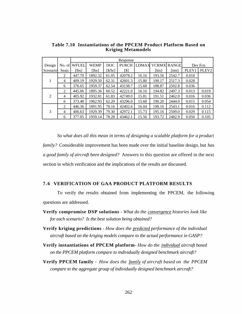
262
Table 7.10 Instantiations of the PPCEM Product Platform Based onKriging Metamodels
ResponseDesign No. of WFUEL WEMP DOC PURCH LDMAX VCRMX RANGE Dev Fcn
Scenario Seats [lbs] [lbs] [$/hr] [$] [kts] [nm] PLEV1 PLEV22 447.70 1892.32 61.05 42078.2 16.16 193.56 2542.7 0.018
1 4 409.19 1929.50 62.31 42601.3 15.80 190.17 2517.3 0.0286 376.65 1959.37 62.54 43138.7 15.68 188.87 2502.8 0.0362 445.06 1895.36 60.52 42221.0 16.16 194.82 2497.3 0.013 0.019
2 4 405.92 1932.81 61.83 42749.0 15.81 191.51 2462.0 0.016 0.0366 373.48 1962.93 62.20 43296.0 15.68 190.20 2444.0 0.015 0.0542 446.36 1891.95 78.16 42402.6 16.04 198.16 2543.1 0.016 0.112
3 4 406.63 1929.39 79.30 42972.1 15.73 195.16 2509.0 0.029 0.1156 377.05 1959.14 78.28 43462.1 15.56 193.72 2482.9 0.050 0.105
So what does all this mean in terms of designing a scalable platform for a product
family? Considerable improvement has been made over the initial baseline design, but has
a good family of aircraft been designed? Answers to this question are offered in the next
section in which verification and the implications of the results are discussed.
7.6 VERIFICATION OF GAA PRODUCT PLATFORM RESULTS
To verify the results obtained from implementing the PPCEM, the following
questions are addressed.
Verify compromise DSP solutions - What do the convergence histories look like
for each scenario? Is the best solution being obtained?
Verify kriging predictions - How does the predicted performance of the individual
aircraft based on the kriging models compare to the actual performance in GASP?
Verify instantiations of PPCEM platform- How do the individual aircraft based
on the PPCEM platform compare to individually designed benchmark aircraft?
Verify PPCEM family - How does the family of aircraft based on the PPCEM
compare to the aggregate group of individually designed benchmark aircraft?
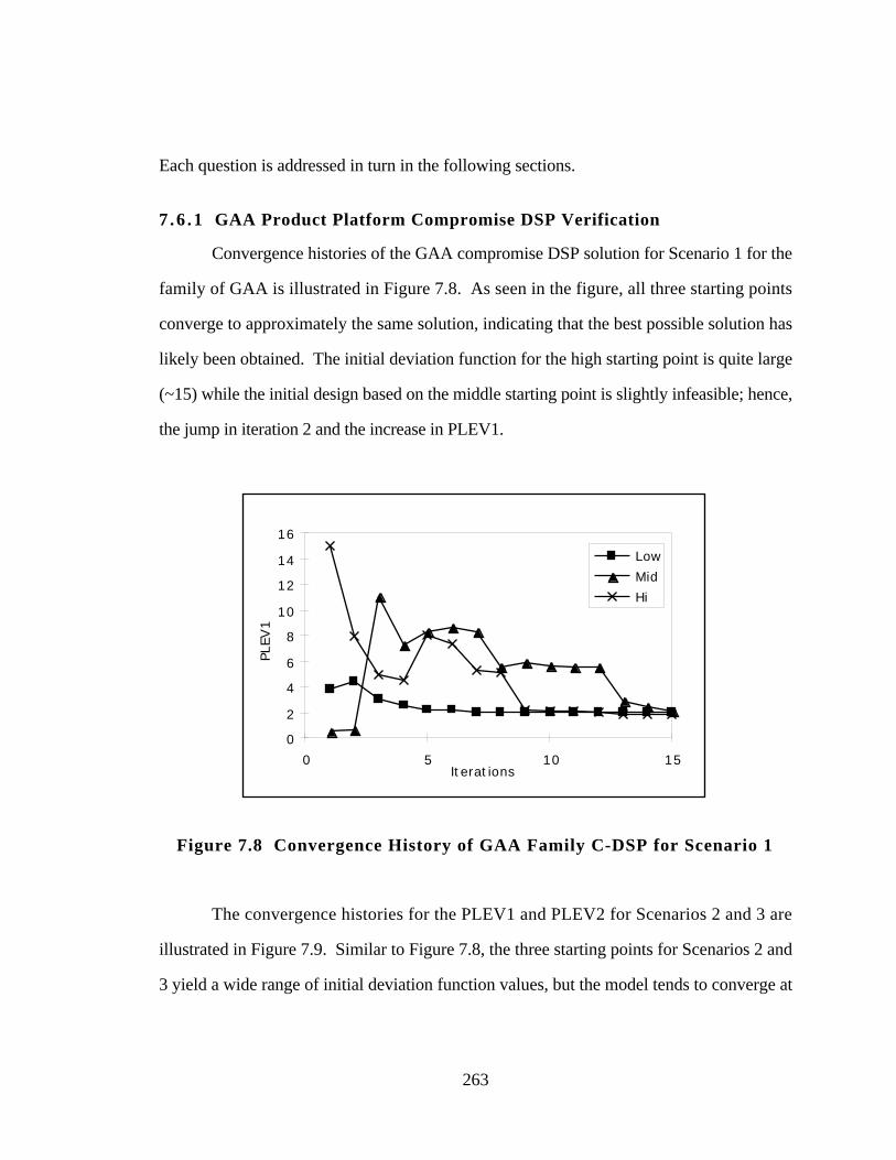
263
Each question is addressed in turn in the following sections.
7 .6 .1 GAA Product Platform Compromise DSP Verification
Convergence histories of the GAA compromise DSP solution for Scenario 1 for the
family of GAA is illustrated in Figure 7.8. As seen in the figure, all three starting points
converge to approximately the same solution, indicating that the best possible solution has
likely been obtained. The initial deviation function for the high starting point is quite large
(~15) while the initial design based on the middle starting point is slightly infeasible; hence,
the jump in iteration 2 and the increase in PLEV1.
0
2
4
6
8
10
12
14
16
0 5 10 15Iterations
PLEV
1
Low
Mid
Hi
Figure 7.8 Convergence History of GAA Family C-DSP for Scenario 1
The convergence histories for the PLEV1 and PLEV2 for Scenarios 2 and 3 are
illustrated in Figure 7.9. Similar to Figure 7.8, the three starting points for Scenarios 2 and
3 yield a wide range of initial deviation function values, but the model tends to converge at
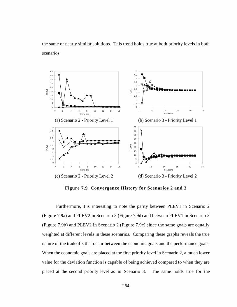
264
the same or nearly similar solutions. This trend holds true at both priority levels in both
scenarios.
0
5
10
15
20
25
30
35
40
45
0 2 4 6 8 10 12 14 16
Iterations
PLEV
1
0
0.5
1
1.5
2
2.5
3
3.5
4
4.5
5
0 5 10 15 20 25
Iterations
PLEV
1
(a) Scenario 2 - Priority Level 1 (b) Scenario 3 - Priority Level 1
0
0.5
1
1.5
2
2.5
3
3.5
4
4.5
5
0 2 4 6 8 10 12 14 16
Iterations
PLEV
2
0
5
10
15
20
25
30
35
40
45
0 5 10 15 20 25
Iterations
PLEV
2
(c) Scenario 2 - Priority Level 2 (d) Scenario 3 - Priority Level 2
Figure 7.9 Convergence History for Scenarios 2 and 3
Furthermore, it is interesting to note the parity between PLEV1 in Scenario 2
(Figure 7.9a) and PLEV2 in Scenario 3 (Figure 7.9d) and between PLEV1 in Scenario 3
(Figure 7.9b) and PLEV2 in Scenario 2 (Figure 7.9c) since the same goals are equally
weighted at different levels in these scenarios. Comparing these graphs reveals the true
nature of the tradeoffs that occur between the economic goals and the performance goals.
When the economic goals are placed at the first priority level in Scenario 2, a much lower
value for the deviation function is capable of being achieved compared to when they are
placed at the second priority level as in Scenario 3. The same holds true for the
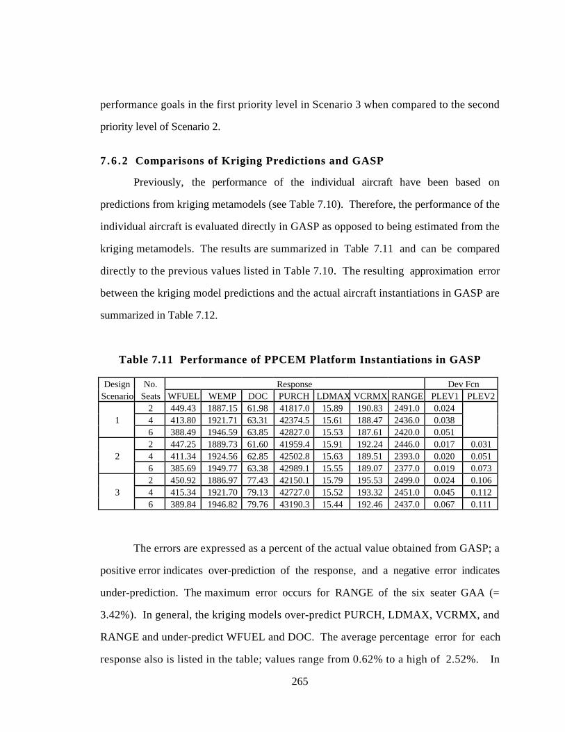
265
performance goals in the first priority level in Scenario 3 when compared to the second
priority level of Scenario 2.
7 .6 .2 Comparisons of Kriging Predictions and GASP
Previously, the performance of the individual aircraft have been based on
predictions from kriging metamodels (see Table 7.10). Therefore, the performance of the
individual aircraft is evaluated directly in GASP as opposed to being estimated from the
kriging metamodels. The results are summarized in Table 7.11 and can be compared
directly to the previous values listed in Table 7.10. The resulting approximation error
between the kriging model predictions and the actual aircraft instantiations in GASP are
summarized in Table 7.12.
Table 7.11 Performance of PPCEM Platform Instantiations in GASP
Design No. Response Dev FcnScenario Seats WFUEL WEMP DOC PURCH LDMAX VCRMX RANGE PLEV1 PLEV2
2 449.43 1887.15 61.98 41817.0 15.89 190.83 2491.0 0.0241 4 413.80 1921.71 63.31 42374.5 15.61 188.47 2436.0 0.038
6 388.49 1946.59 63.85 42827.0 15.53 187.61 2420.0 0.0512 447.25 1889.73 61.60 41959.4 15.91 192.24 2446.0 0.017 0.031
2 4 411.34 1924.56 62.85 42502.8 15.63 189.51 2393.0 0.020 0.0516 385.69 1949.77 63.38 42989.1 15.55 189.07 2377.0 0.019 0.0732 450.92 1886.97 77.43 42150.1 15.79 195.53 2499.0 0.024 0.106
3 4 415.34 1921.70 79.13 42727.0 15.52 193.32 2451.0 0.045 0.1126 389.84 1946.82 79.76 43190.3 15.44 192.46 2437.0 0.067 0.111
The errors are expressed as a percent of the actual value obtained from GASP; a
positive error indicates over-prediction of the response, and a negative error indicates
under-prediction. The maximum error occurs for RANGE of the six seater GAA (=
3.42%). In general, the kriging models over-predict PURCH, LDMAX, VCRMX, and
RANGE and under-predict WFUEL and DOC. The average percentage error for each
response also is listed in the table; values range from 0.62% to a high of 2.52%. In
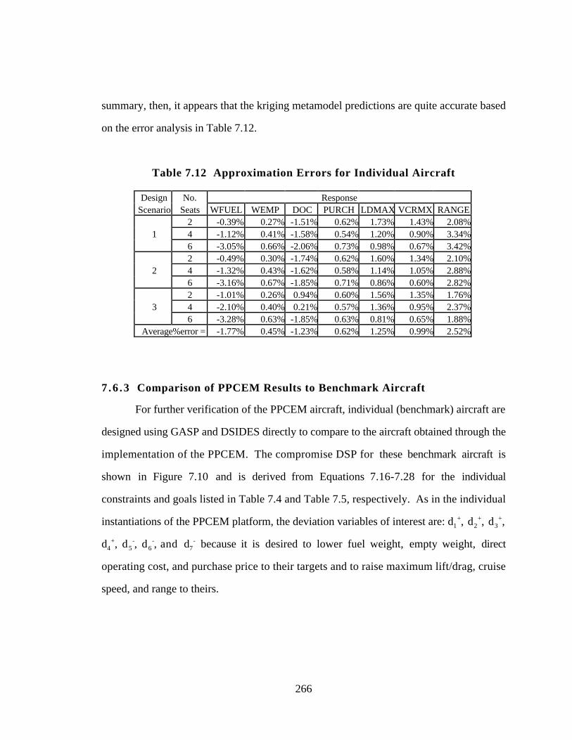
266
summary, then, it appears that the kriging metamodel predictions are quite accurate based
on the error analysis in Table 7.12.
Table 7.12 Approximation Errors for Individual Aircraft
Design No. ResponseScenario Seats WFUEL WEMP DOC PURCH LDMAX VCRMX RANGE
2 -0.39% 0.27% -1.51% 0.62% 1.73% 1.43% 2.08%1 4 -1.12% 0.41% -1.58% 0.54% 1.20% 0.90% 3.34%
6 -3.05% 0.66% -2.06% 0.73% 0.98% 0.67% 3.42%2 -0.49% 0.30% -1.74% 0.62% 1.60% 1.34% 2.10%
2 4 -1.32% 0.43% -1.62% 0.58% 1.14% 1.05% 2.88%6 -3.16% 0.67% -1.85% 0.71% 0.86% 0.60% 2.82%2 -1.01% 0.26% 0.94% 0.60% 1.56% 1.35% 1.76%
3 4 -2.10% 0.40% 0.21% 0.57% 1.36% 0.95% 2.37%6 -3.28% 0.63% -1.85% 0.63% 0.81% 0.65% 1.88%
Average%error = -1.77% 0.45% -1.23% 0.62% 1.25% 0.99% 2.52%
7 .6 .3 Comparison of PPCEM Results to Benchmark Aircraft
For further verification of the PPCEM aircraft, individual (benchmark) aircraft are
designed using GASP and DSIDES directly to compare to the aircraft obtained through the
implementation of the PPCEM. The compromise DSP for these benchmark aircraft is
shown in Figure 7.10 and is derived from Equations 7.16-7.28 for the individual
constraints and goals listed in Table 7.4 and Table 7.5, respectively. As in the individual
instantiations of the PPCEM platform, the deviation variables of interest are: d1+, d2
+, d3+,
d4+, d5
-, d6-, and d7
- because it is desired to lower fuel weight, empty weight, direct
operating cost, and purchase price to their targets and to raise maximum lift/drag, cruise
speed, and range to theirs.
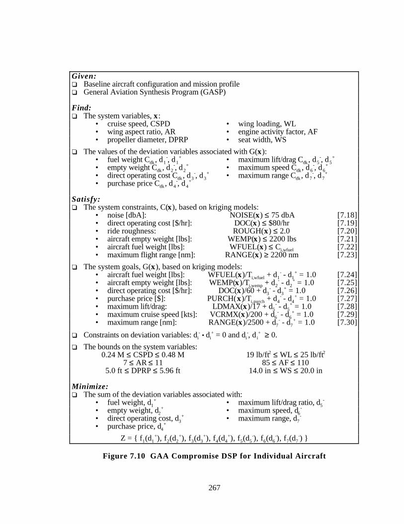
267
Given:❏ Baseline aircraft configuration and mission profile❏ General Aviation Synthesis Program (GASP)
Find:❏ The system variables, x:
• cruise speed, CSPD • wing loading, WL• wing aspect ratio, AR • engine activity factor, AF• propeller diameter, DPRP • seat width, WS
❏ The values of the deviation variables associated with G(x):• fuel weight Cdk , d1
-, d1+ • maximum lift/drag Cdk , d5
-, d5+
• empty weight Cdk , d2-, d2
+ • maximum speed Cdk , d6-, d6
+
• direct operating cost Cdk , d3-, d3
+ • maximum range Cdk , d7-, d7
+
• purchase price Cdk , d4-, d4
+
Satisfy:❏ The system constraints, C(x), based on kriging models:
• noise [dbA]: NOISE(x) ≤ 75 dbA [7.18]• direct operating cost [$/hr]: DOC(x) ≤ $80/hr [7.19]• ride roughness: ROUGH(x) ≤ 2.0 [7.20]• aircraft empty weight [lbs]: WEMP(x) ≤ 2200 lbs [7.21]• aircraft fuel weight [lbs]: WFUEL(x) ≤ Ci,wfuel [7.22]• maximum flight range [nm]: RANGE(x) ≥ 2200 nm [7.23]
❏ The system goals, G(x), based on kriging models:• aircraft fuel weight [lbs]: WFUEL(x)/Ti,wfuel + d1
- - d1+ = 1.0 [7.24]
• aircraft empty weight [lbs]: WEMP(x)/Ti,wemp + d2- - d2
+ = 1.0 [7.25]• direct operating cost [$/hr]: DOC(x)/60 + d3
- - d3+ = 1.0 [7.26]
• purchase price [$]: PURCH(x)/Ti,purch + d4- - d4
+ = 1.0 [7.27]• maximum lift/drag: LDMAX(x)/17 + d5
- - d5+ = 1.0 [7.28]
• maximum cruise speed [kts]: VCRMX(x)/200 + d6- - d6
+ = 1.0 [7.29]• maximum range [nm]: RANGE(x)/2500 + d7
- - d7+ = 1.0 [7.30]
❏ Constraints on deviation variables: di- • di
+ = 0 and di-, d i
+ ≥ 0.
❏ The bounds on the system variables:0.24 M ≤ CSPD ≤ 0.48 M 19 lb/ft2 ≤ WL ≤ 25 lb/ft2
7 ≤ AR ≤ 11 85 ≤ AF ≤ 1105.0 ft ≤ DPRP ≤ 5.96 ft 14.0 in ≤ WS ≤ 20.0 in
Minimize:❏ The sum of the deviation variables associated with:
• fuel weight, d1+ • maximum lift/drag ratio, d5
-
• empty weight, d2+ • maximum speed, d6
-
• direct operating cost, d3+ • maximum range, d7
-
• purchase price, d4+
Z = { f1(d1+), f2(d2
+), f3(d3+), f4(d4
+), f5(d5-), f6(d6
-), f7(d7-) }
Figure 7.10 GAA Compromise DSP for Individual Aircraft
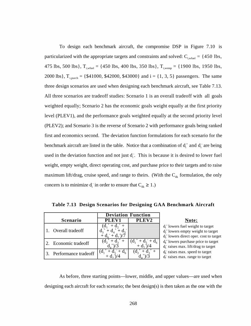
268
To design each benchmark aircraft, the compromise DSP in Figure 7.10 is
particularized with the appropriate targets and constraints and solved: Ci,wfuel = {450 lbs,
475 lbs, 500 lbs}, Ti,wfuel = {450 lbs, 400 lbs, 350 lbs}, Ti,wemp = {1900 lbs, 1950 lbs,
2000 lbs}, T i,purch = {$41000, $42000, $43000} and i = {1, 3, 5} passengers. The same
three design scenarios are used when designing each benchmark aircraft, see Table 7.13.
All three scenarios are tradeoff studies: Scenario 1 is an overall tradeoff with all goals
weighted equally; Scenario 2 has the economic goals weight equally at the first priority
level (PLEV1), and the performance goals weighted equally at the second priority level
(PLEV2); and Scenario 3 is the reverse of Scenario 2 with performance goals being ranked
first and economics second. The deviation function formulations for each scenario for the
benchmark aircraft are listed in the table. Notice that a combination of di+ and di
- are being
used in the deviation function and not just di-. This is because it is desired to lower fuel
weight, empty weight, direct operating cost, and purchase price to their targets and to raise
maximum lift/drag, cruise speed, and range to theirs. (With the Cdk formulation, the only
concern is to minimize di- in order to ensure that Cdk ≥ 1.)
Table 7.13 Design Scenarios for Designing GAA Benchmark Aircraft
Deviation FunctionScenario PLEV1 PLEV2 Note:
1. Overall tradeoff(d1
+ + d2+ +
d3+ + d4
+ + d5-
+ d6- + d7
-)/7
d1+ lowers fuel weight to target
d2+ lowers empty weight to target
d3+ lowers direct oper. cost to target
2. Economic tradeoff (d2+ + d3
+ +d4
+)/3(d1
+ + d5- + d6
-
+ d7-)/4
d4+ lowers purchase price to target
d5- raises max. lift/drag to target
3. Performance tradeoff (d1+ + d5
- + d6-
+ d7-)/4
(d2+ + d3
+ +d4
+)/3d6
- raises max. speed to targetd7
- raises max. range to target
As before, three starting points—lower, middle, and upper values—are used when
designing each aircraft for each scenario; the best design(s) is then taken as the one with the
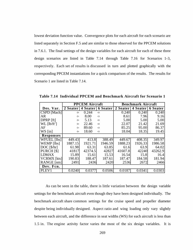
269
lowest deviation function value. Convergence plots for each aircraft for each scenario are
listed separately in Section F.5 and are similar to those observed for the PPCEM solutions
in 7.6.1. The final settings of the design variables for each aircraft for each of these three
design scenarios are listed in Table 7.14 through Table 7.16 for Scenarios 1-3,
respectively. Each set of results is discussed in turn and plotted graphically with the
corresponding PPCEM instantiations for a quick comparison of the results. The results for
Scenario 1 are listed in Table 7.14.
Table 7.14 Individual PPCEM and Benchmark Aircraft for Scenario 1
PPCEM Aircraft Benchmark AircraftDes. Var. 2 Seater 4 Seater 6 Seater 2 Seater 4 Seater 6 Seater
CSPD [Mach] ï 0.244 ð 0.240 0.240 0.240AR ï 8.00 ð 8.61 7.96 9.16DPRP [ft] ï 5.13 ð 5.00 5.00 5.00WL [lb/ft2] ï 22.46 ð 22.07 21.42 21.69AF ï 89.60 ð 85.25 95.00 86.37WS [in] ï 18.60 ð 18.04 18.35 19.45Responses
WFUEL [lbs] 449.43 413.8 388.49 449.67 408.35 349.97WEMP [lbs] 1887.15 1921.71 1946.59 1888.23 1926.33 1986.58DOC [$/hr] 61.98 63.31 63.85 61.6 63.9 64.02PURCH [$] 41817 42374.5 42827 41607.8 42240 43262.9LDMAX 15.89 15.61 15.53 16.54 15.8 16.4VCRMX [kts] 190.83 188.47 187.61 187.47 184.58 181.94RANGE [nm] 2491 2436 2420 2536 2672 2466Dev. Fcn.
PLEV1 0.0240 0.0377 0.0506 0.0187 0.0341 0.0303
As can be seen in the table, there is little variation between the design variable
settings for the benchmark aircraft even though they have been designed individually. The
benchmark aircraft share common settings for the cruise speed and propeller diameter
despite being individually designed. Aspect ratio and wing loading only vary slightly
between each aircraft, and the difference in seat widths (WS) for each aircraft is less than
1.5 in. The engine activity factor varies the most of the six design variables. It is

270
interesting to note that the PPCEM design variable values are quite close to the benchmark
designs. Seat width, aspect ratio, and engine activity factor all are contained within the
range of settings for the benchmark aircraft. The PPCEM values for cruise speed and
propeller diameter are only slightly larger than the corresponding values which are shared
between all three benchmark aircraft.
Despite the similarity of the design variable settings for the two families of aircraft,
only the 4 seater benchmark and PPCEM aircraft have similar deviation function values.
The two and six seater aircraft from the PPCEM are both slightly worse than the
benchmark designs as a result of having a common set of design variables for all three
aircraft. To see why this is and to facilitate comparison of the performance of the two
families of aircraft (the one based on the PPCEM and the group of benchmark aircraft),
plots of the individual goal achievements for each aircraft are given in Figure 7.11 for
Scenario 1. The idea of using a “spider” or “snowflake” plot to show goal achievement
comes from Sandgren (1989). In the spider plot, goal deviation values are plotted on the
axes of the web; the closer a mark is on its axis to the origin, the better that particular goal
has been achieved. In this manner, the shape of the polygon formed by connecting the
deviation values for each design can be used to compare designs quickly. In other words,
the two seater aircraft from the PPCEM platform and the benchmark design can be quickly
compared by plotting their goal achievement on the same spider plot as is done in Figure
7.11 for all three aircraft which comprise the GAA family.
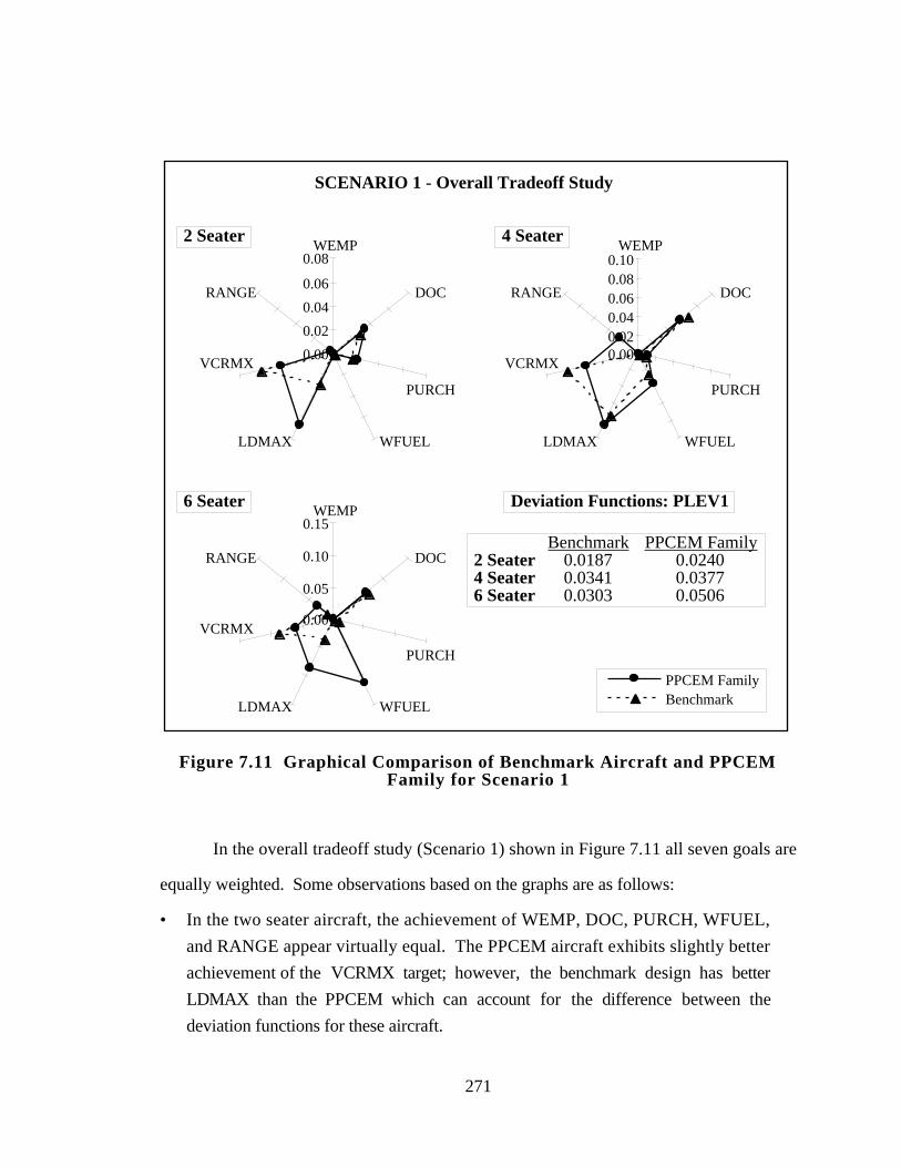
271
PPCEM FamilyBenchmark
SCENARIO 1 - Overall Tradeoff Study
0.00
0.02
0.04
0.06
0.08WEMP
DOC
PURCH
WFUELLDMAX
VCRMX
RANGE
2 Seater
0.000.020.040.060.080.10
WEMP
DOC
PURCH
WFUELLDMAX
VCRMX
RANGE
4 Seater
0.00
0.05
0.10
0.15WEMP
DOC
PURCH
WFUELLDMAX
VCRMX
RANGE
6 Seater
Benchmark PPCEM Family 2 Seater 0.0187 0.0240 4 Seater 0.0341 0.0377 6 Seater 0.0303 0.0506
Deviation Functions: PLEV1
Figure 7.11 Graphical Comparison of Benchmark Aircraft and PPCEMFamily for Scenario 1
In the overall tradeoff study (Scenario 1) shown in Figure 7.11 all seven goals are
equally weighted. Some observations based on the graphs are as follows:
• In the two seater aircraft, the achievement of WEMP, DOC, PURCH, WFUEL,
and RANGE appear virtually equal. The PPCEM aircraft exhibits slightly better
achievement of the VCRMX target; however, the benchmark design has better
LDMAX than the PPCEM which can account for the difference between the
deviation functions for these aircraft.
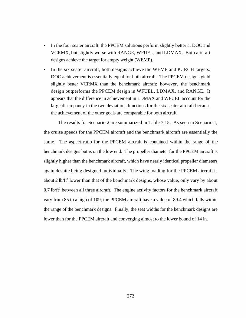
272
• In the four seater aircraft, the PPCEM solutions perform slightly better at DOC and
VCRMX, but slightly worse with RANGE, WFUEL, and LDMAX. Both aircraft
designs achieve the target for empty weight (WEMP).
• In the six seater aircraft, both designs achieve the WEMP and PURCH targets.
DOC achievement is essentially equal for both aircraft. The PPCEM designs yield
slightly better VCRMX than the benchmark aircraft; however, the benchmark
design outperforms the PPCEM design in WFUEL, LDMAX, and RANGE. It
appears that the difference in achievement in LDMAX and WFUEL account for the
large discrepancy in the two deviations functions for the six seater aircraft because
the achievement of the other goals are comparable for both aircraft.
The results for Scenario 2 are summarized in Table 7.15. As seen in Scenario 1,
the cruise speeds for the PPCEM aircraft and the benchmark aircraft are essentially the
same. The aspect ratio for the PPCEM aircraft is contained within the range of the
benchmark designs but is on the low end. The propeller diameter for the PPCEM aircraft is
slightly higher than the benchmark aircraft, which have nearly identical propeller diameters
again despite being designed individually. The wing loading for the PPCEM aircraft is
about 2 lb/ft2 lower than that of the benchmark designs, whose value, only vary by about
0.7 lb/ft2 between all three aircraft. The engine activity factors for the benchmark aircraft
vary from 85 to a high of 109; the PPCEM aircraft have a value of 89.4 which falls within
the range of the benchmark designs. Finally, the seat widths for the benchmark designs are
lower than for the PPCEM aircraft and converging almost to the lower bound of 14 in.
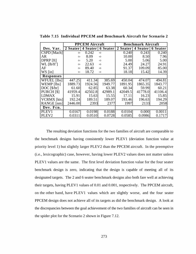
273
Table 7.15 Individual PPCEM and Benchmark Aircraft for Scenario 2
PPCEM Aircraft Benchmark AircraftDes. Var. 2 Seater 4 Seater 6 Seater 2 Seater 4 Seater 6 Seater
CSPD [Mach] ï 0.242 ð 0.240 0.243 0.240AR ï 8.09 ð 10.00 8.50 7.96DPRP [ft] ï 5.20 ð 5.00 5.06 5.00WL [lb/ft2] ï 22.63 ð 24.49 24.27 24.91AF ï 89.40 ð 91.37 109.09 85.00WS [in] ï 18.72 ð 18.18 15.42 14.39Responses
WFUEL [lbs] 447.25 411.34 385.69 450.04 474.07 494.81WEMP [lbs] 1889.73 1924.56 1949.77 1891.95 1865.35 1843.77DOC [$/hr] 61.60 62.85 63.38 60.34 59.99 60.21PURCH [$] 41959.4 42502.8 42989.1 42049.5 41778.0 41106.4LDMAX 15.91 15.63 15.55 17.11 16.23 15.85VCRMX [kts] 192.24 189.51 189.07 193.46 196.63 194.29RANGE [nm] 2446.00 2393 2377 1997 2133 2058Dev. Fcn.
PLEV1 0.0167 0.0198 0.0188 0.0104 0.000 0.0011PLEV2 0.0311 0.0510 0.0728 0.0585 0.0986 0.1717
The resulting deviation functions for the two families of aircraft are comparable to
the benchmark designs having consistently lower PLEV1 (deviation function value at
priority level 1) but slightly larger PLEV2 than the PPCEM aircraft. In the preemptive
(i.e., lexicographic) case, however, having lower PLEV2 values does not matter unless
PLEV1 values are the same. The first level deviation function value for the four seater
benchmark design is zero, indicating that the design is capable of meeting all of its
designated targets. The 2 and 6 seater benchmark designs also both fare well at achieving
their targets, having PLEV1 values of 0.01 and 0.001, respectively. The PPCEM aircraft,
on the other hand, have PLEV1 values which are slightly worse, and the four seater
PPCEM design does not achieve all of its targets as did the benchmark design. A look at
the discrepancies between the goal achievement of the two families of aircraft can be seen in
the spider plot for the Scenario 2 shown in Figure 7.12.
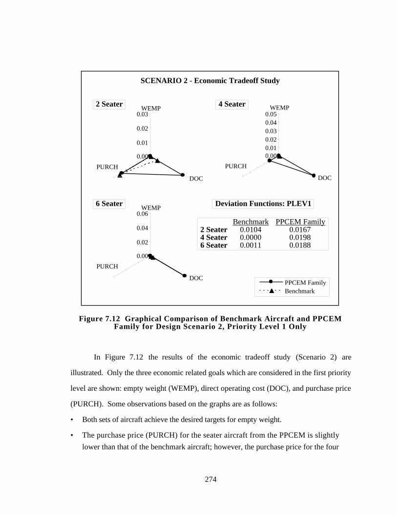
274
0.00
0.02
0.04
0.06WEMP
DOC
PURCH
0.000.010.020.030.040.05
WEMP
DOC
PURCH
0.00
0.01
0.02
0.03WEMP
DOC
PURCH
PPCEM FamilyBenchmark
SCENARIO 2 - Economic Tradeoff Study
2 Seater 4 Seater
6 Seater
Benchmark PPCEM Family 2 Seater 0.0104 0.0167 4 Seater 0.0000 0.0198 6 Seater 0.0011 0.0188
Deviation Functions: PLEV1
Figure 7.12 Graphical Comparison of Benchmark Aircraft and PPCEMFamily for Design Scenario 2, Priority Level 1 Only
In Figure 7.12 the results of the economic tradeoff study (Scenario 2) are
illustrated. Only the three economic related goals which are considered in the first priority
level are shown: empty weight (WEMP), direct operating cost (DOC), and purchase price
(PURCH). Some observations based on the graphs are as follows:
• Both sets of aircraft achieve the desired targets for empty weight.
• The purchase price (PURCH) for the seater aircraft from the PPCEM is slightly
lower than that of the benchmark aircraft; however, the purchase price for the four
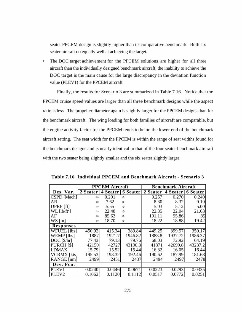
275
seater PPCEM design is slightly higher than its comparative benchmark. Both six
seater aircraft do equally well at achieving the target.
• The DOC target achievement for the PPCEM solutions are higher for all three
aircraft than the individually designed benchmark aircraft; the inability to achieve the
DOC target is the main cause for the large discrepancy in the deviation function
value (PLEV1) for the PPCEM aircraft.
Finally, the results for Scenario 3 are summarized in Table 7.16. Notice that the
PPCEM cruise speed values are larger than all three benchmark designs while the aspect
ratio is less. The propeller diameter again is slightly larger for the PPCEM designs than for
the benchmark aircraft. The wing loading for both families of aircraft are comparable, but
the engine activity factor for the PPCEM tends to be on the lower end of the benchmark
aircraft setting. The seat width for the PPCEM is within the range of seat widths found for
the benchmark designs and is nearly identical to that of the four seater benchmark aircraft
with the two seater being slightly smaller and the six seater slightly larger.
Table 7.16 Individual PPCEM and Benchmark Aircraft - Scenario 3
PPCEM Aircraft Benchmark AircraftDes. Var. 2 Seater 4 Seater 6 Seater 2 Seater 4 Seater 6 Seater
CSPD [Mach] ï 0.291 ð 0.257 0.270 0.240AR ï 7.62 ð 8.30 8.32 9.19DPRP [ft] ï 5.55 ð 5.03 5.12 5.00WL [lb/ft2] ï 22.48 ð 22.35 22.04 21.63AF ï 85.63 ð 101.11 95.86 85WS [in] ï 18.70 ð 18.22 18.88 19.42Responses
WFUEL [lbs] 450.92 415.34 389.84 449.25 399.57 350.17WEMP [lbs] 1887 1921.7 1946.82 1888.8 1937.72 1986.37DOC [$/hr] 77.43 79.13 79.76 68.03 72.92 64.19PURCH [$] 42150 42727 43190.3 41871 42699.8 43237.2LDMAX 15.79 15.52 15.44 16.32 16.05 16.44VCRMX [kts] 195.53 193.32 192.46 190.62 187.99 181.68RANGE [nm] 2499 2451 2437 2494 2497 2478Dev. Fcn.
PLEV1 0.0240 0.0446 0.0671 0.0223 0.0293 0.0335PLEV2 0.1062 0.1120 0.1112 0.0517 0.0772 0.0251
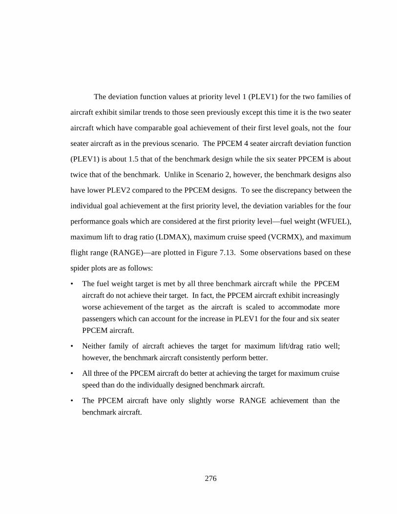
276
The deviation function values at priority level 1 (PLEV1) for the two families of
aircraft exhibit similar trends to those seen previously except this time it is the two seater
aircraft which have comparable goal achievement of their first level goals, not the four
seater aircraft as in the previous scenario. The PPCEM 4 seater aircraft deviation function
(PLEV1) is about 1.5 that of the benchmark design while the six seater PPCEM is about
twice that of the benchmark. Unlike in Scenario 2, however, the benchmark designs also
have lower PLEV2 compared to the PPCEM designs. To see the discrepancy between the
individual goal achievement at the first priority level, the deviation variables for the four
performance goals which are considered at the first priority level—fuel weight (WFUEL),
maximum lift to drag ratio (LDMAX), maximum cruise speed (VCRMX), and maximum
flight range (RANGE)—are plotted in Figure 7.13. Some observations based on these
spider plots are as follows:
• The fuel weight target is met by all three benchmark aircraft while the PPCEM
aircraft do not achieve their target. In fact, the PPCEM aircraft exhibit increasingly
worse achievement of the target as the aircraft is scaled to accommodate more
passengers which can account for the increase in PLEV1 for the four and six seater
PPCEM aircraft.
• Neither family of aircraft achieves the target for maximum lift/drag ratio well;
however, the benchmark aircraft consistently perform better.
• All three of the PPCEM aircraft do better at achieving the target for maximum cruise
speed than do the individually designed benchmark aircraft.
• The PPCEM aircraft have only slightly worse RANGE achievement than the
benchmark aircraft.
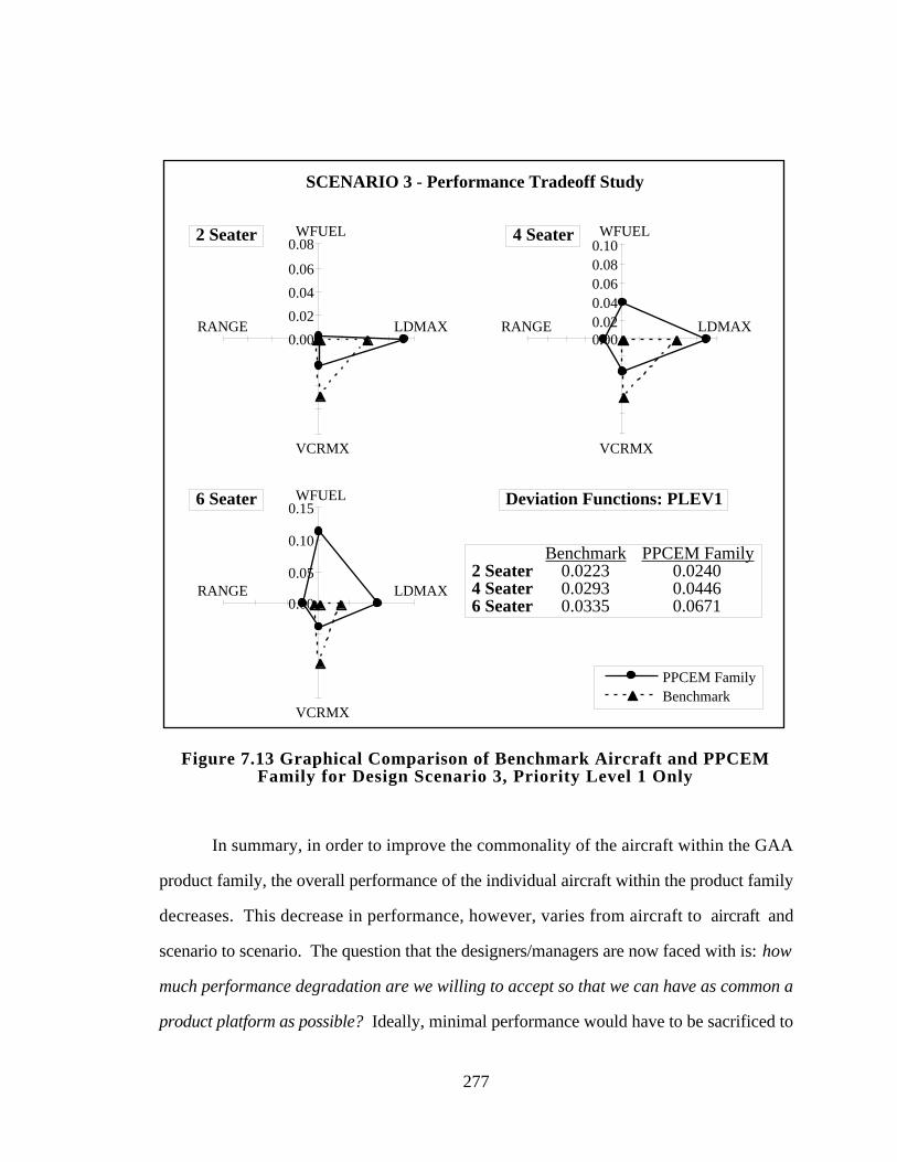
277
PPCEM FamilyBenchmark
SCENARIO 3 - Performance Tradeoff Study
0.000.020.040.060.080.10WFUEL
LDMAX
VCRMX
RANGE
4 Seater
Benchmark PPCEM Family 2 Seater 0.0223 0.0240 4 Seater 0.0293 0.0446 6 Seater 0.0335 0.0671
Deviation Functions: PLEV1 6 Seater
0.00
0.05
0.10
0.15WFUEL
LDMAX
VCRMX
RANGE
2 Seater
0.00
0.02
0.04
0.06
0.08WFUEL
LDMAX
VCRMX
RANGE
Figure 7.13 Graphical Comparison of Benchmark Aircraft and PPCEMFamily for Design Scenario 3, Priority Level 1 Only
In summary, in order to improve the commonality of the aircraft within the GAA
product family, the overall performance of the individual aircraft within the product family
decreases. This decrease in performance, however, varies from aircraft to aircraft and
scenario to scenario. The question that the designers/managers are now faced with is: how
much performance degradation are we willing to accept so that we can have as common a
product platform as possible? Ideally, minimal performance would have to be sacrificed to
278
increase commonality between derivative products, but it appears that a tradeoff does exist
as one might expect. In reality, however, it would not be known how much performance
was being sacrificed by designing a common platform for the product family because
benchmark designs would not necessarily exist (unless this was a redesign process).
Toward this end, a product variety tradeoff study is performed in the next section.
7 .6 .4 Product Variety Tradeoff Study
To assess the tradeoff between product commonality and product performance
within the family of GAA, a product variety tradeoff study is performed using the PDI and
NCI measures described in Section 3.1.5. Currently, there are two points on the PDI vs.
NCI graph: the family of aircraft based on the PPCEM solutions and the group (family) of
benchmark aircraft which have been individually designed. What is interesting to study is
the effect of allowing one or more design variables to vary in the PPCEM for each aircraft
while holding the remaining variables constant at the platform values found using the
PPCEM. In this manner, the PPCEM facilitates generating a variety of alternatives for the
product platform and corresponding product family. By allowing one or more variables to
vary between aircraft, the performance of the individual aircraft within the resulting product
family can be improved such that there is minimal tradeoff between product commonality
and performance. Before this tradeoff can be assessed, however, the relative importance of
the design variables is needed in order to compute NCI for each family of aircraft.
The weightings in NCI used in this study are based on rank ordering the design
variables with regard to relative ease/cost with which they can be allowed to vary—the
more costly it is to allow that variable to change, the more important it is to have that
variable stay the same across derivative products. For this example, the weightings listed
in Table 7.17 are used. Cruise speed (CSPD) is the easiest/cheapest variable to allow to
vary between designs because it is easy to vary the cruise speed throughout the mission
279
without having to make any modifications to the aircraft; meanwhile, seat width (WS) is the
most expensive to allow to vary because it is costly not to have the same fuselage width
(fuselage width being directly proportional to seat width) for all of the aircraft within the
GAA family. These weights are derived from a pairwise comparison of the design
variables; the justification for the pairwise comparison and computation of the rank
ordering and relative importance are explained in Section F.4.1.
Table 7.17 Relative Importance of Design Variables
DesignVariable
RankOrder†
RelativeImportance
AF 3 0.1429AR 5 0.2381
CSPD 1 0.0476DPRP 2 0.0952WL 4 0.1905WS 6 0.2857
† Larger numbers indicate preference.
For this product variety study, two design scenarios are considered: the economic
tradeoff study (Scenario 2) and the performance tradeoff study (Scenario 3) listed in Table
7.13. For these two scenarios, the individual PPCEM and benchmark aircraft are listed in
Table 7.15 and Table 7.16 for Scenarios 2 and 3, respectively. The resulting PDI and NCI
for each group of aircraft based on these design variable values are computed and listed in
Table 7.18 and Table 7.20 for Scenarios 2 and 3, respectively; remember that only the first
priority level is used when computing PDI, and the weightings used in the NCI are the
relative importances listed in Table 7.17 and do not include the variation in the scale factor.
Knowing the two extremes of the PDI vs. NCI curve, it is possible to work
“backward” along the curve from the PPCEM solutions toward the benchmark designs by
280
allowing one or multiple design variables to vary between each aircraft while holding the
others fixed at the PPCEM platform values. This process proceeds as follows:
1. Starting with the individual PPCEM aircraft, vary one variable at a time for each
aircraft; for instance, hold {AF, AR, CSPD, DPRP, WL} at the settings prescribed
by the PPCEM platform and vary WS for each aircraft to improve the performance
of that aircraft as much as possible. This entails solving a compromise DSP for
each aircraft, with the PPCEM value for WS taken as the starting point in DSIDES.
All six variables are allowed to vary one-at-a-time from the PPCEM platform
values, solving a compromise DSP for each aircraft for each variable. NCI and
PDI are then computed for each of the six resulting aircraft families, e.g., the family
of aircraft which share common {AF, AR, CSPD, DPRP, WL} but varying WS.
2. Repeat Step 1, allowing any two variables to vary at a given time between aircraft
from the PPCEM platform values. There are 15 possible pairs of variables which
are varied two-at-a-time, and a compromise DSP is solved for each possible pair
with the PPCEM value taken as the starting point. NCI and PDI are computed for
each of the 15 resulting product families.
3. Repeat Step 1, allowing any three variables to vary at a given time between aircraft.
In order to reduce the number of combinations that must be examined, CSPD is not
varied from aircraft to aircraft because it is known not to change much between
aircraft in the group of benchmark designs. Hence, only AF, AR, DPRP, WL, and
WS are allowed to vary from their PPCEM platform values, resulting in 10
different combinations of the five variables taken three at a time. NCI and PDI are
computed for each of the 10 resulting product families.
In total, (6x3)+(15x3)+(10x3) = 93 compromise DSPs are solved in this product
variety study for each scenario. The resulting NCI and PDI are listed in Table 7.18 for
Scenario 2 and in Table 7.20 for Scenario 3. In the tables, the results are grouped by the
number of variables where the variables not listed are being held constant. For instance, in
Table 7.18 the NCI and PDI for the family of aircraft when allowing WL to vary from one
aircraft to the next are 0.0171 and 0.0155, respectively, with all over design variables fixed
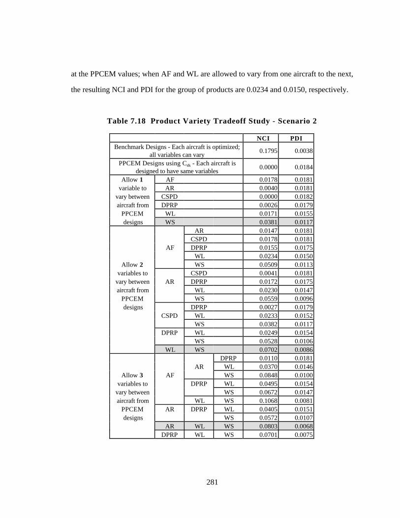
281
at the PPCEM values; when AF and WL are allowed to vary from one aircraft to the next,
the resulting NCI and PDI for the group of products are 0.0234 and 0.0150, respectively.
Table 7.18 Product Variety Tradeoff Study - Scenario 2
NCI PDIBenchmark Designs - Each aircraft is optimized;
all variables can vary0.1795 0.0038
PPCEM Designs using Cdk - Each aircraft isdesigned to have same variables
0.0000 0.0184
Allow 1 AF 0.0178 0.0181variable to AR 0.0040 0.0181
vary between CSPD 0.0000 0.0182aircraft from DPRP 0.0026 0.0179
PPCEM WL 0.0171 0.0155designs WS 0.0381 0.0117
AR 0.0147 0.0181CSPD 0.0178 0.0181
AF DPRP 0.0155 0.0175WL 0.0234 0.0150
Allow 2 WS 0.0509 0.0113variables to CSPD 0.0041 0.0181
vary between AR DPRP 0.0172 0.0175aircraft from WL 0.0230 0.0147
PPCEM WS 0.0559 0.0096designs DPRP 0.0027 0.0179
CSPD WL 0.0233 0.0152WS 0.0382 0.0117
DPRP WL 0.0249 0.0154WS 0.0528 0.0106
WL WS 0.0702 0.0086DPRP 0.0110 0.0181
AR WL 0.0370 0.0146Allow 3 AF WS 0.0848 0.0100
variables to DPRP WL 0.0495 0.0154vary between WS 0.0672 0.0147aircraft from WL WS 0.1068 0.0081
PPCEM AR DPRP WL 0.0405 0.0151designs WS 0.0572 0.0107
AR WL WS 0.0803 0.0068DPRP WL WS 0.0701 0.0075
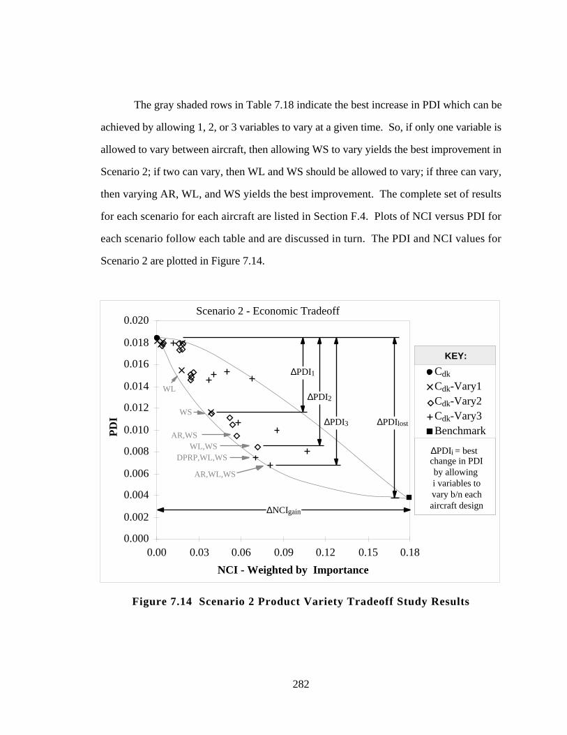
282
The gray shaded rows in Table 7.18 indicate the best increase in PDI which can be
achieved by allowing 1, 2, or 3 variables to vary at a given time. So, if only one variable is
allowed to vary between aircraft, then allowing WS to vary yields the best improvement in
Scenario 2; if two can vary, then WL and WS should be allowed to vary; if three can vary,
then varying AR, WL, and WS yields the best improvement. The complete set of results
for each scenario for each aircraft are listed in Section F.4. Plots of NCI versus PDI for
each scenario follow each table and are discussed in turn. The PDI and NCI values for
Scenario 2 are plotted in Figure 7.14.
∆PDIi = best change in PDIby allowing i variables tovary b/n eachaircraft design
0.000
0.002
0.004
0.006
0.008
0.010
0.012
0.014
0.016
0.018
0.020
0.00 0.03 0.06 0.09 0.12 0.15 0.18
NCI - Weighted by Importance
PD
I
Scenario 2 - Economic Tradeoff
Cdk
Cdk-Vary1Cdk-Vary2Cdk-Vary3Benchmark
∆PDI1
∆PDI2
∆PDI3
KEY:
∆PDIlost
∆NCIgain
WL
WS
WL,WSDPRP,WL,WS
AR,WL,WS
AR,WS
Figure 7.14 Scenario 2 Product Variety Tradeoff Study Results
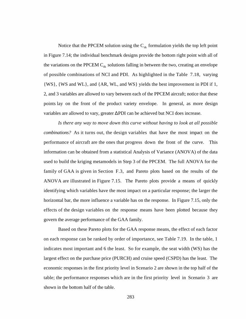
283
Notice that the PPCEM solution using the Cdk formulation yields the top left point
in Figure 7.14; the individual benchmark designs provide the bottom right point with all of
the variations on the PPCEM Cdk solutions falling in between the two, creating an envelope
of possible combinations of NCI and PDI. As highlighted in the Table 7.18, varying
{WS}, {WS and WL}, and {AR, WL, and WS} yields the best improvement in PDI if 1,
2, and 3 variables are allowed to vary between each of the PPCEM aircraft; notice that these
points lay on the front of the product variety envelope. In general, as more design
variables are allowed to vary, greater ∆PDI can be achieved but NCI does increase.
Is there any way to move down this curve without having to look at all possible
combinations? As it turns out, the design variables that have the most impact on the
performance of aircraft are the ones that progress down the front of the curve. This
information can be obtained from a statistical Analysis of Variance (ANOVA) of the data
used to build the kriging metamodels in Step 3 of the PPCEM. The full ANOVA for the
family of GAA is given in Section F.3, and Pareto plots based on the results of the
ANOVA are illustrated in Figure 7.15. The Pareto plots provide a means of quickly
identifying which variables have the most impact on a particular response; the larger the
horizontal bar, the more influence a variable has on the response. In Figure 7.15, only the
effects of the design variables on the response means have been plotted because they
govern the average performance of the GAA family.
Based on these Pareto plots for the GAA response means, the effect of each factor
on each response can be ranked by order of importance, see Table 7.19. In the table, 1
indicates most important and 6 the least. So for example, the seat width (WS) has the
largest effect on the purchase price (PURCH) and cruise speed (CSPD) has the least. The
economic responses in the first priority level in Scenario 2 are shown in the top half of the
table; the performance responses which are in the first priority level in Scenario 3 are
shown in the bottom half of the table.
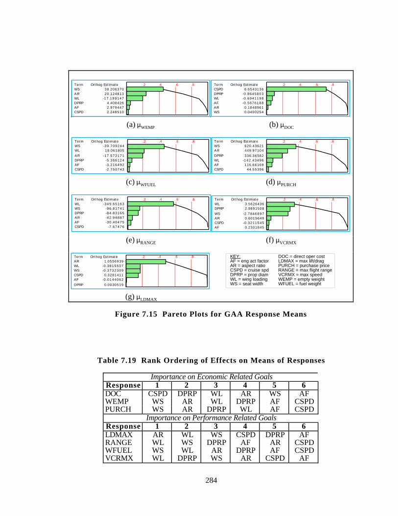
284
TermWSARWLDPRPAFCSPD
Orthog Estimate 38.206370 20.124813-17.199147 4.408426 2.979447 2.248510
.2 .4 .6 .8 TermCSPDDPRPWLAFARWS
Orthog Estimate 6.6543136-0.8645803-0.6941198-0.5676188 0.1848961 0.0400254
.2 .4 .6 .8
(a) µWEMP (b) µDOC
TermWSWLARDPRPAFCSPD
Orthog Estimate-39.709244 18.061805-17.572171 -5.366124 -3.216492 -2.750743
.2 .4 .6 .8 TermWSARDPRPWLAFCSPD
Orthog Estimate 620.43621 449.97104 336.36582-142.43496 116.66169 44.55396
.2 .4 .6 .8
(c) µWFUEL (d) µPURCH
TermWLWSDPRPARAFCSPD
Orthog Estimate-349.65163 -96.81741 -84.83165 -42.94887 -30.40475 -7.67476
.2 .4 .6 .8 TermWLDPRPWSARCSPDAF
Orthog Estimate 3.5626436 2.9891508-2.7846897 0.6015649-0.3211545 0.2301845
.2 .4 .6 .8
(e) µRANGE (f) µVCRMX
TermARWLWSCSPDAFDPRP
Orthog Estimate 1.0556939-0.3815507-0.3732309 0.3281411-0.0144062 0.0030519
.2 .4 .6 .8 KEY: DOC = direct oper costAF = eng act factor LDMAX = max lift/dragAR = aspect ratio PURCH = purchase priceCSPD = cruise spd RANGE = max flight rangeDPRP = prop diam VCRMX = max speedWL = wing loading WEMP = empty weightWS = seat width WFUEL = fuel weight
(g) µLDMAX
Figure 7.15 Pareto Plots for GAA Response Means
Table 7.19 Rank Ordering of Effects on Means of Responses
Importance on Economic Related GoalsResponse 1 2 3 4 5 6DOC CSPD DPRP WL AR WS AFWEMP WS AR WL DPRP AF CSPDPURCH WS AR DPRP WL AF CSPD
Importance on Performance Related GoalsResponse 1 2 3 4 5 6LDMAX AR WL WS CSPD DPRP AFRANGE WL WS DPRP AF AR CSPDWFUEL WS WL AR DPRP AF CSPDVCRMX WL DPRP WS AR CSPD AF
285
Returning to the tradeoff study for Scenario 2, the design variables that shape the
front of the envelope when allowed to vary are as follows: WS, WL, {AR,WS},
{WS,WL}, {WS, WL, DPRP}, and {AR, WL, WS}. Looking at the rank ordering of
importance in Table 7.19, it can be seen that the variables in these combinations are
variables that have the largest effect on the responses. WS has the largest effect on WEMP
and PURCH, two of the three economic responses in Scenario 2; {WS, AR} are the two
most important factors both of these economic responses; {AR, WL, WS} are among the
top three variables that are most important to the three economic responses in Scenario 2.
Thus, by allowing the design variables with the most impact to vary between aircraft while
keeping the others fixed, substantial improvements in performance can be obtained.
To see if the same holds true in Scenario 3, the NCI and PDI values for Scenario 3
are listed in Table 7.20 and plotted in Figure 7.16. As highlighted in the table, the best
improvement in PDI can be obtained by allowing AR to vary between aircraft if only one
variable is allowed to vary. Notice in Table 7.19 that AR is most important to LDMAX.
Recall from Figure 7.13 that the largest discrepancy between the PPCEM family of aircraft
and the benchmark group of aircraft is the achievement of LDMAX. By allowing AR to
vary between aircraft within the PPCEM family, each aircraft is able to achieve better
LDMAX, resulting in a lower PDI for the PPCEM product family. Meanwhile, if two
variables are allowed to vary, then AF and WL yield the best improvement in PDI because
WL has a large impact on both RANGE and VCRMX. In the three variable case, varying
DPRP, WL, and WS yield the best improvement; notice that all three of these variables are
among the most influential variables on the performance responses as shown in Table 7.19.
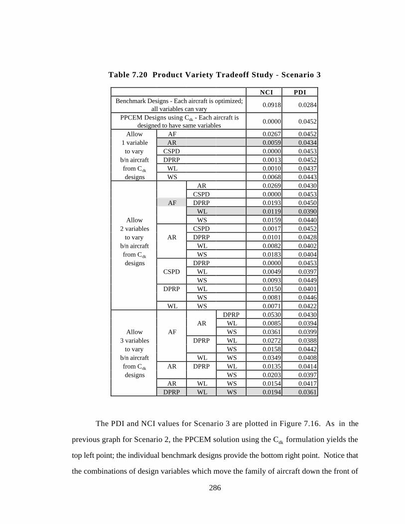
286
Table 7.20 Product Variety Tradeoff Study - Scenario 3
NCI PDIBenchmark Designs - Each aircraft is optimized;
all variables can vary0.0918 0.0284
PPCEM Designs using Cdk - Each aircraft isdesigned to have same variables
0.0000 0.0452
Allow AF 0.0267 0.04521 variable AR 0.0059 0.0434to vary CSPD 0.0000 0.0453
b/n aircraft DPRP 0.0013 0.0452from Cdk WL 0.0010 0.0437designs WS 0.0068 0.0443
AR 0.0269 0.0430CSPD 0.0000 0.0453
AF DPRP 0.0193 0.0450WL 0.0119 0.0390
Allow WS 0.0159 0.04402 variables CSPD 0.0017 0.0452
to vary AR DPRP 0.0101 0.0428b/n aircraft WL 0.0082 0.0402from Cdk WS 0.0183 0.0404designs DPRP 0.0000 0.0453
CSPD WL 0.0049 0.0397WS 0.0093 0.0449
DPRP WL 0.0150 0.0401WS 0.0081 0.0446
WL WS 0.0071 0.0422DPRP 0.0530 0.0430
AR WL 0.0085 0.0394Allow AF WS 0.0361 0.0399
3 variables DPRP WL 0.0272 0.0388to vary WS 0.0158 0.0442
b/n aircraft WL WS 0.0349 0.0408from Cdk AR DPRP WL 0.0135 0.0414designs WS 0.0203 0.0397
AR WL WS 0.0154 0.0417DPRP WL WS 0.0194 0.0361
The PDI and NCI values for Scenario 3 are plotted in Figure 7.16. As in the
previous graph for Scenario 2, the PPCEM solution using the Cdk formulation yields the
top left point; the individual benchmark designs provide the bottom right point. Notice that
the combinations of design variables which move the family of aircraft down the front of
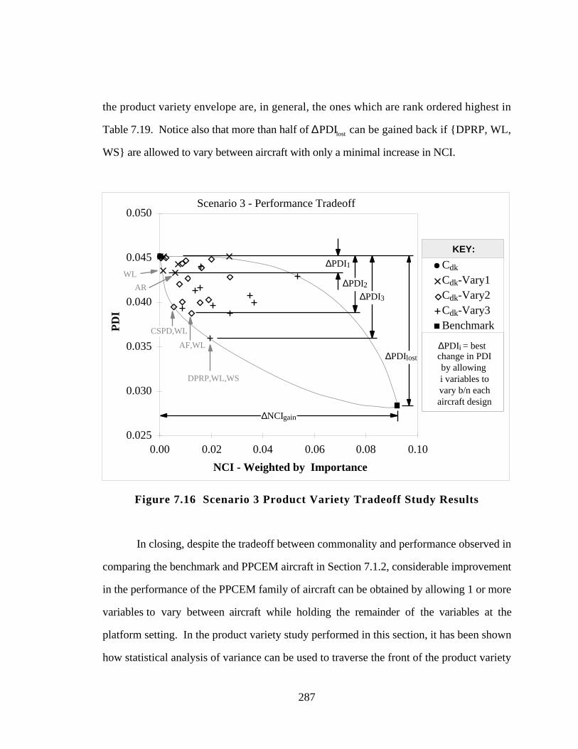
287
the product variety envelope are, in general, the ones which are rank ordered highest in
Table 7.19. Notice also that more than half of ∆PDIlost can be gained back if {DPRP, WL,
WS} are allowed to vary between aircraft with only a minimal increase in NCI.
0.025
0.030
0.035
0.040
0.045
0.050
0.00 0.02 0.04 0.06 0.08 0.10
NCI - Weighted by Importance
PD
I
Scenario 3 - Performance Tradeoff
∆PDI1
∆PDI2∆PDI3
∆PDIi = best change in PDIby allowing i variables tovary b/n eachaircraft design
Cdk
Cdk-Vary1Cdk-Vary2Cdk-Vary3Benchmark
KEY:
∆PDIlost
∆NCIgain
WL
AR
DPRP,WL,WS
CSPD,WL
AF,WL
Figure 7.16 Scenario 3 Product Variety Tradeoff Study Results
In closing, despite the tradeoff between commonality and performance observed in
comparing the benchmark and PPCEM aircraft in Section 7.1.2, considerable improvement
in the performance of the PPCEM family of aircraft can be obtained by allowing 1 or more
variables to vary between aircraft while holding the remainder of the variables at the
platform setting. In the product variety study performed in this section, it has been shown
how statistical analysis of variance can be used to traverse the front of the product variety
288
tradeoff envelope, maximizing the gains in PDI with minimal loss in commonality. It is
now up to the discretion of the designers/managers to evaluate the implications of this
tradeoff on inventory, production, and sales to decide the appropriate compromise between
commonality and performance. A closer look at some of the lessons learned from this
example is offered in the next section along with a summary of the chapter.
7.7 LESSONS LEARNED: A LOOK BACK AND A LOOK AHEAD
In this chapter, the PPCEM is applied in full to the design of a family of General
Aviation aircraft. The GAA family is based on a common scalable product platform which
is scaled around the number of passengers in much the same way that Boeing has scaled
their 747 series of aircraft around the capacity and flight range (cf., Rothwell and Gardiner,
1990). The market segmentation grid has been used to help identify an appropriate
leveraging strategy for the family of aircraft based on the initial problem statement, i.e.,
horizontally leverage the family of GAA to satisfy a variety of low-end market segments.
Each aircraft eventually could be vertically scaled as well through the addition and removal
of features as technology improves to increase its performance and attractiveness to a mid-
range or high-end customer base.
Particularization of the PPCEM for this example occurs through GASP, the General
Aviation Synthesis Program, which is used to model and simulate the performance of each
aircraft mathematically . Kriging metamodels for response means and variances are
employed within the PPCEM to facilitate the implementation of robust design based on
GASP analyses. These kriging metamodels then are used in conjunction with design
capability indices and a GAA compromise DSP to synthesize a robust aircraft platform
which is scalable into a family of aircraft.
Three different design scenarios are used to exercise the GAA compromise DSP to
create alternative product platforms and the product platform portfolio. Instantiation of the
289
individual aircraft within the PPCEM family reveals that the PPCEM provides an effective
means for designing a common scalable aircraft platform for the family of GAA.
However, upon comparison with individually designed benchmark aircraft, a tradeoff is
found to exist between having a common set of design variables which define the aircraft
platform and the performance of the scaled derivatives based on that platform. To examine
the extent to which this tradeoff occurs, a product variety tradeoff study is performed using
the PPCEM to demonstrate the ease with which alternative product platforms and product
families can be generate and to make use of the NCI and PDI measures proposed in Section
3.1.5. It is observed that considerable improvement can be made by allowing one or more
variables to vary between each aircraft based on the original PPCEM platform; however,
commonality between the aircraft is sacrificed. To determine which variables to vary,
ANOVA of the data used to build the kriging metamodels in Step 3 of the PPCEM can be
used to determine the variables that have the largest effect on each response, allowing the
front portion of the product variety envelope to be traversed for maximum improvement in
PDI with minimal loss of commonality. The implications of this tradeoff on inventory,
production, and sales must be considered in order to decide upon an appropriate
compromise between commonality and performance. However, the purpose of the
PPCEM is to facilitate generating a variety of alternatives for the common product platform
and corresponding product platform and not to select one from them.
A summary of the hypotheses tested in this example is as follows:
Hypothesis 1 - The PPCEM is employed in this chapter to design a family of aircraft
based on a common scalable product platform. The success of the method to
improve the baseline design and generate a variety of alternatives for the GAA
platform as discussed in Sections 7.5 and 7.6 provides further verification of
Hypothesis 1.
Sub-Hypothesis 1.1 - The market segmentation grid is utilized in Section 7.1.3 to
help identify an appropriate (horizontal) scale factor for the family of GAA—the
290
number of passengers—in order to achieve the desired platform leveraging based
on the problem objectives; this further supports Sub-Hypothesis 1.1.
Sub-Hypothesis 1.2 - The scale factor for the GAA product family is the number of
passengers, see Sections 7.1.3 and 7.2. Robust design principles then are used in
this example to develop an aircraft platform—defined by six design variables—
which is insensitive to variations in the scale factor and is thus good for the family
of General Aviation aircraft based on the two, four, and six seater configurations.
The success of this implementation helps to support Sub-Hypothesis 1.2.
Sub-Hypothesis 1 .3 - Design capability indices are utilized in this example to
aggregate individual targets and constraints and to facilitate the design of a family of
General Aviation aircraft. Combining this formulation with the compromise DSP
allows a family of GAA to be designed around a common, scalable product
platform, further verifying Sub-Hypothesis 1.3.
Hypothesis 2 - Kriging metamodels are utilized to facilitate the implementation of the
design capability indices and expedite the search for a suitable product platform for
the family of GAA. Validation of the kriging metamodels in Section 7.3 and 7.6.2
indicates that the kriging models are sufficiently accurate to benefit the PPCEM.
So, are the solutions obtained from the PPCEM useful? The PPCEM has been
used to generate a variety of feasible options for the GAA platform and corresponding
family of aircraft. While there is some tradeoff between the performance of the individual
aircraft based on the PPCEM platform when compared to a family of individually designed
benchmark aircraft, the increased commonality between the design specifications of each
aircraft (i.e., aspect ratio, seat width, propeller diameter, etc.) should generate sufficient
savings to offset the minimal loss in performance. Regardless of whether it does or not,
the family of aircraft obtained using the PPCEM yields considerable improvement over the
initial family of aircraft based on the baseline Beechcraft Bonanza design, see Table 7.8 and
the discussion thereafter.
Are the time and resources consumed within reasonable limits? Basically, the
PPCEM has been used to design a family of three aircraft almost as efficiently as a single

291
aircraft. The initial start up costs to use the PPCEM in this example are about one day
which is the time it takes to sample the GAA design space and construct kriging
metamodels to approximate GASP. Once this is accomplished, the computational savings
resulting from using the PPCEM are significant in two regards:
• computational efficiency gained by using kriging metamodels instead of GASP, and
• design efficiency gained by using the PPCEM to design a family of aircraft
simultaneously around a common scalable platform.
As a result, the computational savings are comparable to, if not greater than, those obtained
in the universal electric motor example in Chapter 6. Consider, for instance, that it requires
approximately 45 seconds to complete one “run” of GASP on a Unix-based SparcServer
670 MP. Meanwhile, the kriging metamodels require approximately 0.25 seconds to run
after about a minute of “pre-processing” which is done automatically prior to optimization.
The savings from using metamodels in the PPCEM are substantial when one considers the
large numbers of design scenarios and tradeoff studies used in this chapter and in Appendix
F, not to mention the fact that multiple starting points are used in all cases. The cost
savings (in terms of number of analysis) are not as clear cut as they are in the universal
motor example in Chapter 6 (see Section 6.5.3); therefore, they are not estimated.
However, the discussion in (Simpson, 1995) regarding the cost savings of using
approximations to replace GASP sheds some light on the magnitude of these savings.
Is the work grounded in reality? As stated in Section 7.1.3, the baseline design
(i.e., starting point) for the GAA product family is the Beechcraft Bonanza B36TC
presented in Section 7.1.3. While the Beechcraft Bonanza is only a six seater aircraft, its
specifications are employed in GASP to provide a family of baseline to compare with the
PPCEM family of aircraft based on a common scalable platform. Discussion of these
results in Section 7.5.1 reveals that the PPCEM solutions are able to improve upon both the
technical and economic performance characteristics of this family of baseline aircraft
292
significantly. While these improvements are slightly less than the improvements obtained
by individually designing each aircraft (i.e., the benchmark designs), the time savings
resulting from using the PPCEM to design the family of three aircraft simultaneously can
be used to “tweak” the individual designs as needed to ensure adequate performance and
product quality. It still stands, however, that the PPCEM solutions, even with all six
design variables held at the common product platform specifications, yield improvement
over the baseline design. The results of the product variety tradeoff studies discussed in
Section 7.6.4 provides several options to improve the PPCEM family of aircraft.
Finally, do the benefits of the work outweigh the cost? The true benefit from using
the PPCEM in a problem like this is the wealth of information that is obtained during its
implementation. The PPCEM greatly facilitates the generation of a variety of alternatives
for a common product platform and its corresponding scaled derivative products. Use of
the PPCEM permits the product platform and the scaled product family to be designed
simultaneously, thus increasing the commonality of specifications across the products
within the family. Product variety tradeoff studies can be easily performed using the
PPCEM (and NCI and PDI metrics) to evaluate the compromise between commonality and
individual product performance, yielding a variety of options for the company to pursue.
This concludes the second, and final, example for testing and verifying the PPCEM
having demonstrated the full implementation of the PPCEM to design a family of products
and facilitate product variety tradeoff studies. In the next and final chapter, a summary of
achievements and contributions from the work is offered along with critical review of the
research and a discussion of possible avenues of future work.
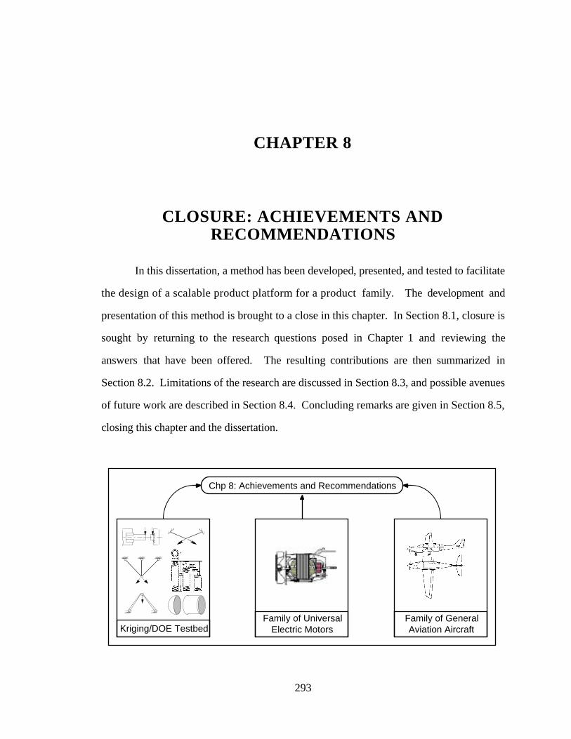
293
8. CHAPTER 8
CLOSURE: ACHIEVEMENTS ANDRECOMMENDATIONS
In this dissertation, a method has been developed, presented, and tested to facilitate
the design of a scalable product platform for a product family. The development and
presentation of this method is brought to a close in this chapter. In Section 8.1, closure is
sought by returning to the research questions posed in Chapter 1 and reviewing the
answers that have been offered. The resulting contributions are then summarized in
Section 8.2. Limitations of the research are discussed in Section 8.3, and possible avenues
of future work are described in Section 8.4. Concluding remarks are given in Section 8.5,
closing this chapter and the dissertation.
Chp 8: Achievements and Recommendations
Family of General Aviation AircraftKriging/DOE Testbed
Family of UniversalElectric Motors

294
8.1 CLOSURE: ANSWERING THE RESEARCH QUESTIONS
As stated in the introduction to Chapter 1, the principal objective in this dissertation
is to develop the Product Platform Concept Exploration Method (PPCEM) to facilitate the
design of a common product platform which can be scaled to realize a product family. In
particular, the concept of platform scalability is introduced and exploited in the context of
the following motivating research question.
Q1. How can a common scalable product platform be modeled and designed for a
product family?
Two secondary research questions are also offered in Section 1.3.1 for investigation in this
dissertation in conjunction with the primary research question.
Q2. Is kriging a viable metamodeling technique for building approximations of
deterministic computer analyses?
Q3. Are space filling designs better suited for building approximations of
deterministic computer analyses than classical experimental designs?
To address these questions, research hypotheses and posits are introduced and
identified in support of achieving the principal objective for the dissertation. Their
elaboration and verification have provided the context in which the research work has
proceeded. The end result is a synthesis of engineering design, operations research,
applied statistics, and strategic management methods and tools to form the Product
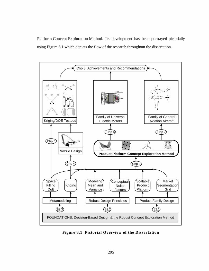
295
Platform Concept Exploration Method. Its development has been portrayed pictorially
using Figure 8.1 which depicts the flow of the research throughout the dissertation.
Nozzle Design
Chp 8: Achievements and Recommendations
Family of General Aviation AircraftKriging/DOE Testbed
Family of UniversalElectric Motors
Metamodeling
ModelingMean andVariance
Robust Design Principles
ConceptualNoise
Factors
ScalableProductPlatform
MarketSegmentation
Grid
Product Family Design
KrigingSpaceFillingDoE
Chp 6
Chp 4 Chp 3
§2.2§2.3 §2.1
Chp 5
Chp 7
FOUNDATIONS: Decision-Based Design & the Robust Concept Exploration Method
Platform
Product Platform Concept Exploration Method
Figure 8.1 Pictorial Overview of the Dissertation
296
Answering Question 1: Question 1 is the primary research question posed for
the work in this dissertation and its answer is embodied by the Product Platform Concept
Exploration Method: a Method which facilitates the synthesis and Exploration of a common
Product Platform Concept which can be scaled into an appropriate family of products. The
method consists of a prescription for formulating the problem and a description for solving
it. Application of the method is demonstrated by means of two examples, namely,
• the design of a universal electric motor platform which is (vertically) scaled around
the stack length of the motor to realize a family of electric motors capable of
satisfying a variety of torque and power requirements (Chapter 6), and
• the design of a General Aviation aircraft platform which is (horizontally) scaled into
a two, a four, and a six seat configuration to realize a family of aircraft capable of
satisfying a variety of performance and economic requirements (Chapter 7).
While only demonstrated for these two examples, it is asserted that the method is generally
applicable to other examples in this class of problems: parametrically scalable product
platforms whose performance can be mathematically modeled or simulated. Other
examples which have taken advantage of this type of scaling include the design of a family
of oil filters (Seshu, 1998) and the design of a family of absorption chillers for a variety of
refrigeration capacities (Hernandez, et al., 1998). Both examples integrate nicely within
the framework of the PPCEM.
In support of the primary research question and objective, three additional questions
also are offered in Section 1.3.1. Answers to these questions are summarized as follows.
Q1.1. How can product platform scaling opportunities be identified from overall
design requirements?
297
In this research, the market segmentation grid (Meyer, 1997) is employed to help
identify platform scaling opportunities based on overall design requirements. Its success as
an attention directing tool for mapping scaling opportunities within a product family is
discussed in Section 2.2.1 and then demonstrated in both examples. In the universal motor
example in Chapter 6, the market segmentation grid is used to identify vertical scaling
opportunities within the desired product family to realize a range of torque and power
ratings for different price/performance tiers within the market; standardization of the motor
interfaces will provide horizontal leveraging opportunities of this family of motors into
other market segments in a manner similar to Black & Decker’s response to Double
Insulation in the 1970s (Lehnerd, 1987). Meanwhile, in the General Aviation aircraft
example in Chapter 7, a horizontal leveraging strategy is identified by means of the market
segmentation grid, resulting in a family of three aircraft based on a two, four, and six seater
configuration leveraged about a common product platform. Opportunities for vertical
scaling of the resulting family of aircraft through engine upgrades, add-on features, and
technological advancements also are discussed; however, none of these features are
implemented in this example.
Q1.2. How can robust design principles be used to facilitate designing a common
scalable product platform?
By identifying “conceptual noise” factors around which a family of products can be
scaled, robust design principles can be abstracted for use in product family and product
platform design. Consequently, the idea of a scale factor is introduced in Section 2.3.2 as
a factor around which a product platform can be “scaled” or “stretched” to realize derivative
products within a product family. Scale factors are, in essence, noise factors for a scalable
298
product platform, and robust design principles can be used accordingly to minimize the
sensitivity of the product platform to variations in these scale factors. Implementation of
this approach is demonstrated through the two examples. In the universal motor example
in Chapter 6, the stack length of the motor is taken as the (parametric) scale factor around
which a family of motors is created. In the General Aviation Aircraft example, the number
of passengers is the (configurational) scale factor around which a family of three aircraft are
developed. In both cases, robust design principles are employed to develop a common set
of design variables which are robust with respect to variations in the scaling factor as the
product platform is scaled and instantiated to realize the product family. A product variety
tradeoff study also is performed in the General Aviation aircraft example (see Section
7.6.2) to further verify this approach.
Q1.3. How can individual targets for derivative products be aggregated and
modeled for product platform design?
Through the identification of appropriate scaling factors during the product family
design process, the individual targets for derivative products can be aggregated into a mean
and variance around which the product family can be simultaneously designed either by
having separate goals for “bringing the mean on target” and “minimizing the variation” or
through the formulation and implementation of appropriate design capability indices to
measure the capability of a family of designs to satisfy a ranged set of design requirements.
The former approach is utilized to design the universal electric motor platform in Chapter 6.
Goals for “bringing the mean on target” and “minimizing the variation” caused by
variations in the scale factor (stack length) are used within a compromise DSP to effect a
platform design which matches the target mean and variation for the aggregated product
299
family. In Chapter 7, design capability indices are employed to design a family of General
Aviation aircraft around a common platform which is instantiated to seat 2, 4, and 6
passengers.
Answering Question 2: Since its introduction into the literature as a useful
metamodeling tool for engineering design by Sacks, et al. (1989), kriging has received little
attention by the engineering community building surrogate models. Perhaps this is because
of the added complexity of fitting the model or using it or of the inability to glean useful
information directly from the MLE parameters used to fit the model. Whatever the reason,
the research in this dissertation has been directed at improving the ease with which kriging
models can be built, validated, and used. Moreover, the initial feasibility study and
comparison of kriging models—with a global underlying constant—with second-order
response surface models in Chapter 4 and the extensive kriging/DOE investigation in
Chapter 5 is aimed at familiarizing the reader with kriging and making it a viable alternative
for building surrogate metamodels of deterministic computer experiments. Its utility was
tested extensively in Chapter 5 wherein it was concluded that the Gaussian correlation
function provides the most accurate kriging predictor, on average, and that kriging can
accurate model a wide variety of functions typical of engineering analysis. While the study
is not all inclusive, nor is it intended to be, it has provided valuable insight into the utility of
kriging metamodels for engineering design. Potential avenues of future work to extend this
promising metamodeling alternative are discussed in Section 8.4.1.
Answering Question 3: As discussed in Section 2.4.3, many researchers argue
that classical experimental designs are not well suited for sampling computer experiments
which are deterministic; rather, points should be chosen to “fill the space,” providing good
coverage of the design space since replicate sample points are not needed. In an effort to
verify the utility of space filling experimental designs, a comparison of nine space filling
and two classical experimental designs is performed in Chapter 5 (see Section 5.4 in

300
particular) to address this third research question. The eleven experimental designs are
compared on the basis of their capability to produce accurate kriging metamodels for the
testbed of six engineering problems used in this dissertation. For the sample sizes
investigated in this study, it was observed that the space filling experimental designs
yielded more accurate kriging models in the larger design spaces (3 and 4 variables) while
the classical experimental designs (CCDs) performed well in the two dimensional design
space for the reasons discussed at the end of Section 5.4.4. Prior to this investigation, few
researchers had compared their experimental designs against one another, or to classical
designs for that matter. As such, the findings in the kriging/DOE study in Chapter 5
represent unique contributions from the research. A summary of the research contributions
is offered in the next section.
8.2 ACHIEVEMENTS: REVIEW OF RESEARCH CONTRIBUTIONS
The contributions offered in this dissertation are introduced in Section 1.3.2 and
realized throughout the dissertation. As stated at the beginning of Chapter 1, the primary
contribution from this work is embodied in the Product Platform Concept Exploration
Method which provides a method to identify, model, and synthesis scalable product
platforms for a product family. The other contributions can be summarized as follows:
Contributions Related to Hypothesis 1 and Sub-Hypotheses 1.1-1.3:
• A procedure for identifying scale factors for a product platform, see Sections 3.1.1
and 3.1.2.
• An abstraction of robust design principles for realizing scalability in product family
design, see Sections 3.1.2 and 3.1.4.
• Non-commonality and performance deviation indices for performing product
variety tradeoff studies, see Sections 3.1.5 and 7.6.2.
Contributions Related to Hypothesis 2:
301
• An algorithm to build, validate, and use a kriging model, see Section 2.4.2,
Chapter 4 and 5, and Appendix A.
• A preliminary comparison of the predictive capability of second-order response
surfaces and kriging models in the design of a rocket nozzle, see Section 4.2.
• An extensive investigation of the effect of five different spatial correlation functions
on the accuracy of a kriging model, see Sections 2.4.2 and Chapter 5.
Contributions Related to Hypothesis 3:
• An extensive investigation of the effect of eleven different sampling strategies on
building an accurate kriging model, see Sections 2.4.3 and Chapter 5.
• An algorithm for generating minimax Latin hypercube designs, see Section 2.4.3
and Appendix C.
What is the value of these contributions? These contributions must be of sufficient
worth to be either an addition to the fundamental knowledge of the field or a new and better
interpretation of the facts already known. The contributions associated with kriging
represent a new interpretation of facts already known. Kriging has been around since the
1960s (see, e.g., Cressie, 1993; Matheron, 1963) when it was developed originally for
mining and geostatistics applications; however, it has received limited attention in the
engineering design community until recently. The kriging algorithm presented is not totally
unique to this dissertation; however, the use of a simulated annealing algorithm (see
Appendix A for more details on its use in the maximum likelihood estimation for the
kriging metamodels) to find the “best” kriging model is. Moreover, the comparison of the
accuracy of different correlation functions on the resulting kriging model had never been
performed in such depth. Likewise, the comparison of space filling and experimental
designs represents a new and better interpretation of facts already known because such an
extensive study has never been undertaken. With the exception of the minimax Latin
hypercube design, the experimental designs investigated in this dissertation are the result of
years of research work by statisticians and mathematicians. The minimax Latin hypercube
302
design, however, represents an addition to the fundamental knowledge of the field of
experimental design.
The contributions made in the area of product family design, specifically the method
of designing scalable product platforms, represents an addition to the fundamental
knowledge of the field. While other product family design strategies and methods have
been slowly evolving, the investigation of a method for platform scaling is previously
unrecorded. The incorporation of the market segmentation grid into the engineering design
process provides a new interpretation of facts already known, demonstrating how the
market segmentation grid becomes a useful attention directing tool for identifying platform
leveraging strategies in product family and, with a little engineering knowledge, appropriate
scale factors for the intended scalable platform. In this regard, the concept of scale factors
in product family design and extending robust design to product family and product
platform design is unique to this dissertation as are the NCI and PDI measures for product
family non-commonality and performance deviation. The measures are not of significant
value in and of themselves, however, the product variety tradeoff studies which these
indices make possible provide significant insight into the tradeoffs of product family
design. Taken together, the resulting Product Platform Concept Exploration Method for
designing scalable product platforms for a product family provides an addition to the
fundamental knowledge of the nascent field of product family design. However, the
PPCEM is by no means a panacea for product platform and product family design nor is it
without its limitations. Toward this end, a critical evaluation of the work is offered in the
next section followed by recommendations for future work in Section 8.4.
8.3 CRITICAL ANALYSIS: LIMITATIONS OF THE RESEARCH
This section comprises the confessional portion of the dissertation wherein the
research itself is critically evaluated. Already the PPCEM has been critically evaluated as it
303
pertains to the two example problems in Chapters 6 and 7, see Sections 6.5 and 7.6.5. In
this section, the critical evaluation is applied to the work as a whole.
So what is really necessary for the PPCEM to be applied to the design of a product
family based on a common scalable product platform? There are two basic requirements
which must be met in order for the PPCEM to be applicable to the design of a scalable
product platform. First, the concept of scalability must be exploitable within the product
family; exploited in the sense that having one or more scale factors provides a means to
realize a variety of performance requirements while also facilitating the manufacturing
process. For instance, in the electric motor example in Chapter 6, the motor could have
just as easily been scaled in the radial dimension as it was in the axial direction (i.e., stack
length) to achieve the necessary torque requirements; however, the underlying assumption
in the choice of stack length as the scale factor is that it can be exploited from both a
technical sense and a manufacturing sense. As Lehnerd (1987) alludes to in his article on
Black & Decker and their universal motor platform, by varying only the stack length of the
motor, all of the motors—ranging from 60 Watts to 660 Watts—could be produced on the
same machine simply by stacking more laminations onto the field and armature. Had the
radius of the motor been scaled instead of the stack length, different machines and tooling
configurations would have been required to produce the family of motors since varying the
radius of the motors is more than a stacking operation. Consequently, it is very important
that one or multiple scale factors be identified for the product family and that it be capable
of being exploited from both a technical standpoint and a manufacturing standpoint in order
for the PPCEM to yield useful results.
The second consideration when applying the PPCEM is that the performance of the
product family must be able to mathematically modeled, simulated, or quantified in order
for the PPCEM to be employed. It would be extremely difficult, if not impossible, for the
PPCEM to be utilized to design a common scalable automotive body platform based solely
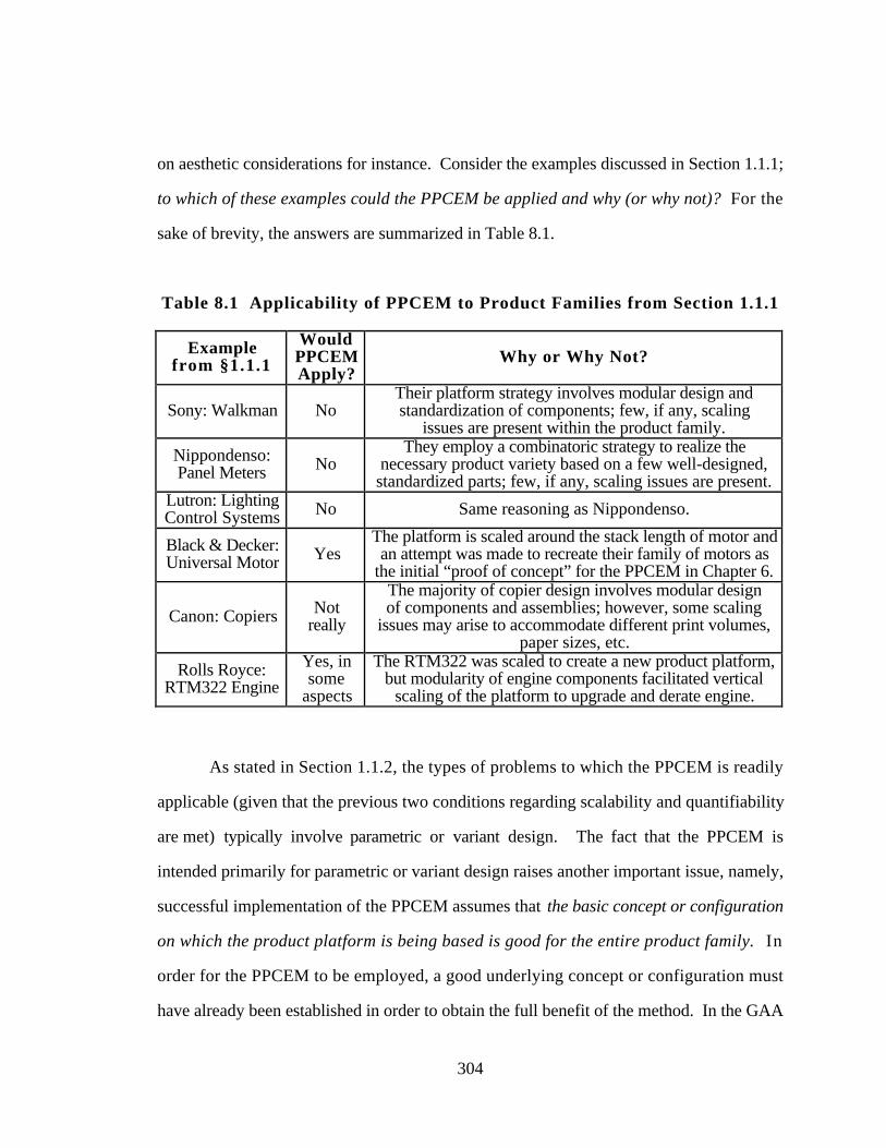
304
on aesthetic considerations for instance. Consider the examples discussed in Section 1.1.1;
to which of these examples could the PPCEM be applied and why (or why not)? For the
sake of brevity, the answers are summarized in Table 8.1.
Table 8.1 Applicability of PPCEM to Product Families from Section 1.1.1
Examplefrom §1.1.1
WouldPPCEMApply?
Why or Why Not?
Sony: Walkman NoTheir platform strategy involves modular design andstandardization of components; few, if any, scaling
issues are present within the product family.
Nippondenso:Panel Meters No
They employ a combinatoric strategy to realize thenecessary product variety based on a few well-designed,standardized parts; few, if any, scaling issues are present.
Lutron: LightingControl Systems No Same reasoning as Nippondenso.
Black & Decker:Universal Motor Yes
The platform is scaled around the stack length of motor andan attempt was made to recreate their family of motors as
the initial “proof of concept” for the PPCEM in Chapter 6.
Canon: Copiers Notreally
The majority of copier design involves modular designof components and assemblies; however, some scaling
issues may arise to accommodate different print volumes,paper sizes, etc.
Rolls Royce:RTM322 Engine
Yes, insome
aspects
The RTM322 was scaled to create a new product platform,but modularity of engine components facilitated vertical
scaling of the platform to upgrade and derate engine.
As stated in Section 1.1.2, the types of problems to which the PPCEM is readily
applicable (given that the previous two conditions regarding scalability and quantifiability
are met) typically involve parametric or variant design. The fact that the PPCEM is
intended primarily for parametric or variant design raises another important issue, namely,
successful implementation of the PPCEM assumes that the basic concept or configuration
on which the product platform is being based is good for the entire product family. In
order for the PPCEM to be employed, a good underlying concept or configuration must
have already been established in order to obtain the full benefit of the method. In the GAA
305
example in Chapter 7, for instance, if the three blade, high wing position, retractable
landing gear configuration had not been a suitable concept for the two, four, and six seater
aircraft, then no matter what parameter settings were obtained from using the PPCEM, the
performance of the family of aircraft would have been poor regardless because the
underlying concept was not good for all three aircraft. An attempt to identify a good
configuration for the family of GAA is discussed in (Simpson, 1995) but the existence of
such a concept is assumed to already exist in this work. Incorporation of the conceptual
and configurational design of the product family along with the parametric scaling of the
product platform is a fertile area for future work.
Furthermore, it is important to keep in mind that the PPCEM facilitates generating
options for common product platforms which can be scaled into an appropriate product
family. The PPCEM is not necessarily intended to be used to evaluate these options or
select one of them. The idea behind the product platform portfolio—the output from
applying the PPCEM—is to maintain sufficient design flexibility to accommodate a wide
variety of customer requirements for as long as possible. As the product platform design
progresses into the detailed stages of design, this design freedom is reduced; however,
during the early stages of the design process, formulating and answering a variety of "what
if" type questions and examining a wide variety of design scenarios is important to the
product platform design process.
Meanwhile, the NCI and PDI measures introduced in Section 3.1.5 and employed
in Section 7.6.4 represent an attempt to provide a means to evaluate different product
platforms and their respective product families. Ultimately the non-commonality of a set of
parameters would be linked to corresponding savings in manufacturing costs and
performance deviation to losses in customer sales; however, this is extremely difficult to
accomplish without sufficient industry input. Modeling the process and manufacturing
306
aspects of product platforms and product families is another fertile research area which has
yet to be explored.
As far as the scale factors themselves goes, the concept of a scale factor—while
discussed in Section 2.3.2 and 3.1.2—is still not fully understood. In the motor example
in Chapter 6, for instance, the mean and standard deviation of the motor stack length was a
scale factor which was treated much like a design variable. Meanwhile, in the GAA
example in Chapter 7, the scale factor was the number of passengers which was treated as a
design parameter which varied from two to six, i.e., its permissible range of values was
known a priori based on the intended leveraging strategy. In any event, when metamodels
are to be utilized within the PPCEM, an initial range for each scale factor is necessary in
order to construct these metamodels. This follows in the same manner that a permissible
range of any noise factor is expected to be known before robust design principles can be
applied to a problem (cf., Phadke, 1989). It is important to examine the concept of scale
factors further, finding more examples of scaled product platforms to understand the
manner in which they have been scaled and, more importantly, how those scale factors are
identified during the design process.
This brings to light another shortcoming of the PPCEM, namely, the use of the
market segmentation grid to “identify” scale factors around which the product platform is
leveraged within a product family. As stated in Section 2.2.1, the market segmentation
grid is only an attention directing tool and considerable engineering “know-how” and
problem insight are required before a successful platform leveraging strategy can be
identified. Then, only after a suitable platform leveraging strategy is identified, can
engineers hope to find (and be able to exploit) scaling opportunities within the product
family to realize the necessary product variety. The market segmentation grid is the end
result of this process and is really only useful for mapping the resulting platform leveraging
strategy. The two examples used in this dissertation trivialize this process when in reality it
307
is extremely difficult, if not impossible, to identify one or more scaling factors which can
be exploited within a product family. Developing tools and methods to facilitate the
process of identifying scale factors is one potential avenue for further investigation.
Part of understanding scale factors better involves understanding their effect on
product performance and how scale factors can be used effectively to satisfy a wide variety
of customer requirements. If scale factors induce too much variability in product
performance, then it might not be possible to apply the PPCEM to develop a common
product platform which does not significantly compromise the performance of the product
family over the range of interest. In such a case, it might be necessary to “split” the design
space into two or more product platforms and corresponding product families rather than
compromise product performance and quality by having one single product platform which
is scaled over the entire range of performance. The work in (Chang and Ward, 1995;
Lucas, 1994; Rangarajan, 1998; Seshu, 1998) further investigates and discusses these
types of issues. Lucas (1994) in particular presents interesting remarks on how to resolve
these types of issues using concepts from robust design as mentioned in Section 2.3.2.
Turning to specific implementation issues within the PPCEM, it may not have been
sufficiently clear that kriging, while part of the PPCEM, is not an integral part of the
PPCEM since it is not the only metamodeling technique which can be used within the
PPCEM. Response surfaces, neural nets, radial basis functions, etc. are all viable
metamodeling options for use in engineering design and with the PPCEM. The extensive
literature review of metamodeling applications in engineering design in (Simpson, et al.,
1997b) supports this. The most important consideration when using metamodels as
surrogate approximations in engineering design is that they are sufficiently accurate for the
task at hand.
The investigations into kriging in this dissertation are primarily intended to shed
light on alternative metamodeling techniques which offer some advantages to response
308
surface models which are typically employed. The case for investigating alternatives to
response surfaces has been made in Section 2.4.1 and is also discussed in (Simpson, et al.,
1998; Simpson, et al., 1997b). The objective in this research is not to prove that kriging
metamodels are better than response surface models; rather, it is to demonstrate that kriging
metamodels are a viable alternative for building surrogate approximations of deterministic
computer analysis.
Similarly, the use of space filling experimental designs as opposed to classical
designs are not mandated by this research. The investigation served to gain a better
understanding of the different sampling strategies which exist and the associated
advantages and disadvantages of each. If one experimental design type had proven
superior in every example, then perhaps only that design should be considered in the
future. However, that was not the case, and the results of this study are by no means
generalizable to all types of engineering design problems. Very few engineering problems,
for instance, involve only two to four variables, and the availability of codes to generate
these space filling designs, the computation expense of them, and the nature of the
underlying analyses are just a few of the key factors that influence the decision of how to
sample a design space efficiently and effectively. Recommendations for future work in the
areas of experimental design and kriging are discussed in more detail in the next section.
8.4 RECOMMENDATIONS: AVENUES OF FUTURE WORK
8.4 .1 Potential Avenues of Future Work in Metamodeling
While extensive in nature, the experimental design study offered in Chapter 5 is by
no means complete nor is it intended to be. Obviously, a wider variety problems should be
considered in order to obtain more generalizable recommendations. Additional space filling
and classical experimental designs which have not been considered include the following:
309
Classical Experimental Designs: fractional factorial designs and small central
composite designs (see, e.g., Box and Draper, 1987); D-optimal designs (see, e.g.,
Box and Draper, 1971; Giunta, et al., 1994; Mitchell, 1974; St. John and Draper,
1975); I-, A-, E-, and G-optimal designs (see, e.g., Hardin and Sloane, 1993;
Myers and Montgomery, 1995); minimum bias designs (see, e.g., Myers and
Montgomery, 1995; Venter and Haftka, 1997); and other hybrid designs (see, e.g.,
Giovannitti-Jensen and Myers, 1989; Myers and Montgomery, 1995)
Space Filling Experimental Designs: median Latin hypercubes (see, e.g.,
Kalagnanam and Diwekar, 1997; McKay, et al., 1979); minimax and maximin
designs (Johnson, et al., 1990); scrambled nets (Koehler and Owen, 1996);
orthogonal arrays of different strengths (Owen, 1992); Maximum entropy designs
(Currin, et al., 1991; Shewry and Wynn, 1987; Shewry and Wynn, 1988); and
factorial hypercube designs (Salagame and Barton, 1997).
In addition to including a wider array of experimental designs and sampling
strategies in the current testbed of problems, larger problems also should be investigated
because very few engineering problems only have 2-4 variables. However, problems with
larger dimensional design spaces (i.e., more design variables), invoke new complications.
For instance, many of the generators used to create the space filling experimental designs
become computationally expensive in and of themselves for large numbers of factors. For
example, the simulated annealing algorithm for generating maximin Latin hypercube
designs (Morris and Mitchell, 1992; 1995) becomes extremely slow even for four factor
designs with as few as 25 variables as discussed in Section 5.1. Moreover, fractional
factorial based central composite designs are available for problems with five or more
factors. Hence, larger problems require different classes of designs all together.
As for the minimax Latin hypercube design, which is unique to this dissertation, the
genetic algorithm which is employed to generate these designs needs further studying to
develop a better understanding of its workings and to learn the optimal combination of
parameters for their use, namely, population size, number of permissible generations,

310
mutation rates, and termination criteria. Also, as it stands right now, the current design
criterion—minimize the maximum distance between sample points and prediction points—
does not yield a unique design for a given sample size and number of design variables.
Developing and implementing an optimization criterion such as that proposed by Mitchell
and Morris (1995) for their maximin Latin hypercube designs could improve the
effectiveness of the minimax Latin hypercubes.
As for kriging, only kriging metamodels which employ an underlying constant for
the global portion of the model have been investigated in this work. In general, f(x) in
Equation 2.14 could be taken as a linear or quadratic model instead of a constant which
may permit more accurate kriging approximations; however, the problem of having a
sufficient number of samples to estimate all of the unknown coefficients in f(x) resurfaces.
A preliminary investigation of such an approach is documented in (Giunta, et al., 1998);
they find that minimal improvement in the accuracy of the kriging approximations is
obtained for their analyses.
Meanwhile, the power of kriging lies in its capability to interpolate accurately a
wide range of linear and non-linear functions. An iterative or sequential strategy which
takes advantage of this may prove useful provided the kriging models can be fit and
validated quickly from one iteration to the next. Consequently, trust region based
approaches which incorporate approximations are being developed by researchers in an
effort to capitalize on the potential of kriging metamodels (see, e.g., Alexandrov, et al.,
1997; Booker, et al., 1996; Booker, et al., 1995; Cox and John, 1995; Dennis and
Torczon, 1996; Osio and Amon, 1996; Schonlau, et al., 1997).
Finally, alternative optimization algorithms for finding the “best” kriging model also
must be investigated for use with larger problems. The simulated annealing algorithm
currently employed to fit the kriging models, see Appendix A, becomes extremely
inefficient for problems with more than eight variables and approximately 180 sample
311
points. Moreover, the matrix inversion routines in the current prediction software do not
take full advantage of the properties of the correlation matrix, R, in kriging which is always
symmetric and positive definite. Several matrix decomposition and inversion algorithms
have been developed to take advantage of these properties; however, they have not been
exploited in this work.
8 .4 .2 Future Work in Product Family and Product Platform Design
The concept of scalability and scalable product platforms has provided an excellent
inroads into product family and product platform design, marrying current research efforts
in Decision-Based Design, the Robust Concept Exploration Method, and robust design
with tools from marketing/management science. The end result is the Product Platform
Concept Exploration Method which has been demonstrated by means of two examples: the
design of a family of universal motors and the design of a family of General Aviation
aircraft. While it has been shown that the PPCEM is effective at producing a family of
products based on scaled instantiations of a product platform, verification through
additional applications will help to further verify the method and improve it.
Furthermore, much in the same way that the product platform provides a platform
for leveraging with a product family, the Product Platform Concept Exploration Method
provides a platform for leveraging future work in product family and product platform
design, see Figure 8.2. The different types of systems can be classified on the vertical axis
of a market segmentation grid and different characteristics of product platform design on
the horizontal axis. The use of the PPCEM to design scalable product platforms for a
variety of systems then can be plotted on this market segmentation grid as illustrated in
Figure 8.2 for the two examples in this dissertation. Perhaps through the addition of
different “Processors” to the PPCEM, additional capabilities could be developed within the
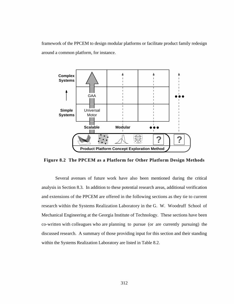
312
framework of the PPCEM to design modular platforms or facilitate product family redesign
around a common platform, for instance.
ComplexSystems
SimpleSystems
Scalable
UniversalMotor
GAA
Platform
Product Platform Concept Exploration Method
Modular
...
??
...
Figure 8.2 The PPCEM as a Platform for Other Platform Design Methods
Several avenues of future work have also been mentioned during the critical
analysis in Section 8.3. In addition to these potential research areas, additional verification
and extensions of the PPCEM are offered in the following sections as they tie to current
research within the Systems Realization Laboratory in the G. W. Woodruff School of
Mechanical Engineering at the Georgia Institute of Technology. These sections have been
co-written with colleagues who are planning to pursue (or are currently pursuing) the
discussed research. A summary of those providing input for this section and their standing
within the Systems Realization Laboratory are listed in Table 8.2.
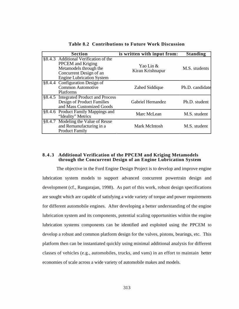
313
Table 8.2 Contributions to Future Work Discussion
Section is written with input from: Standing§8.4.3 Additional Verification of the
PPCEM and KrigingMetamodels through theConcurrent Design of anEngine Lubrication System
Yao Lin &Kiran Krishnapur M.S. students
§8.4.4 Configuration Design ofCommon AutomotivePlatforms
Zahed Siddique Ph.D. candidate
§8.4.5 Integrated Product and ProcessDesign of Product Familiesand Mass Customized Goods
Gabriel Hernandez Ph.D. student
§8.4.6 Product Family Mappings and“Ideality” Metrics Marc McLean M.S. student
§8.4.7 Modeling the Value of Reuseand Remanufacturing in aProduct Family
Mark McIntosh M.S. student
8 .4 .3 Additional Verification of the PPCEM and Kriging Metamodelsthrough the Concurrent Design of an Engine Lubrication System
The objective in the Ford Engine Design Project is to develop and improve engine
lubrication system models to support advanced concurrent powertrain design and
development (cf., Rangarajan, 1998). As part of this work, robust design specifications
are sought which are capable of satisfying a wide variety of torque and power requirements
for different automobile engines. After developing a better understanding of the engine
lubrication system and its components, potential scaling opportunities within the engine
lubrication systems components can be identified and exploited using the PPCEM to
develop a robust and common platform design for the valves, pistons, bearings, etc. This
platform then can be instantiated quickly using minimal additional analysis for different
classes of vehicles (e.g., automobiles, trucks, and vans) in an effort to maintain better
economies of scale across a wide variety of automobile makes and models.
314
In addition to applying the PPCEM to the preliminary design of engine lubrication
components, the use of kriging metamodels for building surrogate approximations of the
associated complex fluid dynamics analyses also can be investigated. Currently second-
order response surfaces are used extensively during the design process; however, the
complex analyses for friction losses, power losses, etc. cannot be modeled well by
response surfaces over a large region of the design space, thus limiting the search for good
solutions. Building accurate global approximations of these analyses using kriging
metamodels may yield additional insight into the complexities of the design space, allowing
better solutions to be identified. The utility of the kriging for partitioning and screening
large systems also can be examined in the context of the engine lubrication system since a
large number of factors (≈ 20) currently are being utilized which would push the limits of
the kriging metamodeling software (i.e., fitting the model, matrix inversion, etc.). Finally,
additional metamodeling techniques such as neural networks (see, e.g., Cheng and
Titterington, 1994; Hajela and Berke, 1992; Rumelhart, et al., 1994; Widrow, et al., 1994)
also can be compared to kriging given the size and complexity of the problem.
8 .4 .4 Configuration Design of Common Automotive Platforms
Balancing the need to customize products for target markets while enabling the
economies of scale of a “world car” is a challenge faced by every automotive manufacturer.
A proliferation of options and model derivatives leads to increased tooling cost and
production line complexity. At first glance, it may appear that automotive platforms are
prime examples for product variety design research. However, in a recent study, Siddique,
et al. (1998) identified significant differences between the variety characteristics of
automotive platforms from some of the examples that other researchers have studied (e.g.,
the Sony Walkman family). For example, the majority of product family design research is
applicable to products that are modular with respect to functions as discussed in Section
315
2.2.3. The automotive platform, on the other hand, is not modular because the platform
accomplishes one function as a whole. As a result, many product family design
approaches do not readily apply; however, careful commonization of platforms can still be
used to increase product variety while reducing the number of components between
different models and the product line complexity.
Developing a common platform requires a robust platform that can support all of the
requirements for different car models and also a common assembly process that can
support these variations. For the automotive industry, platform requirements come from
packaging constraints (underhood, passenger, etc.), safety/crash requirements, size of the
vehicle, styling, and other requirements/regulations. Cars in similar classes have similar
types of requirements (except for styling, maybe); as such, the underbody for similar cars
have the potential to be commonized. Toward this end, a method for the configuration
design of common product platforms is to be developed, extending the parameter design
capabilities of the PPCEM for designing scalable product platforms. As discussed in
(Siddique, 1998; Siddique and Rosen, 1998), this includes the following:
• identification of different product family design concepts and investigation of the
applicability of these concepts towards automotive platform design,
• development of a representation scheme for automotive platform commonization,
• development of a scheme to measure commonality for automotive platforms, and
• establishment of configuration design methods for developing common product
platforms.
Using configuration design methods, the underlying common core for different platforms
can be identified along with the required variations. This information then can be used to
increase the commonality of the product platform and determine how to isolate the
variability in specific modules.
316
In addition to having a common product platform, a commonized assembly process
also is desired so that the same assembly line can be used to produce all of the (minor)
platform derivatives. Using the same component loading sequences, tooling sequences,
etc. provides some of the requirements when developing a common assembly process (cf.,
Nevins and Whitney, 1989; Whitney, 1993). Other requirements that need to be
considered specifically for automobile platforms include common locators, weld lines,
transfer points, etc. Hence, it is imperative to integrate product and process design of
product families.
8 .4 .5 Integrated Product and Process Design of Product Families andMass Customized Goods
Mass customization, i.e., the manufacture of customized products with the
efficiency and speed of mass produced systems, is increasingly recognized as a source of
competitive advantage and possibly the next world-class manufacturing paradigm.
Although the marketplace is rapidly moving towards mass customization, very little work
has been done on formalizing an integrated product and process development method that
would enable companies to practice mass customization in a systematic and efficacious
manner. For example, the PPCEM provides a method to develop a common product
platform which can be scaled to provide the necessary variety for a product family;
however, its focus is solely on modeling the product itself. Meanwhile, research in
flexible, agile, and/or reconfigurable manufacturing systems (see, e.g., Abair, 1995;
Anderson and Pine, 1997; Chinnaiah, et al., 1998; Dhumal, et al., 1996; Hormozi, 1994;
Richards, 1996) focuses primarily on developing cost effective manufacturing systems to
realize a wide variety of products. Integrating the two fields of research has received little
attention in the context of designing families of products.
Mass customization places an onus on companies to integrate closely their various
activities in order to respond quickly to an environment of continuous change. Thus,

317
emphasis should be given to the integration of product design, production system design,
and organization design. The key areas to be addressed include the following:
• Principles of product and process development for mass customized production:
- systematic product and process evolution based on optimization techniques,
parameterization, modularity, standardization, commonality, scalability, and
robustness,
- concurrent design of flexible product and process architectures, and
- optimal design under uncertain demand and customer requirements.
• Structuring design projects for mass customized production:
- identifying appropriate organizational structuring based on the notion of multi-
functional design teams and the particular requirements of mass customized
production, and
- systems to support the required information transfer and group decision
making.
• Design for dis-aggregated production, i.e., decentralized supply chains and
production systems for the growing global economy.
An initial investigation into the concurrent modeling of product and process for
design of make-to-order customized systems is discussed in (Hernandez, et al., 1998)
wherein the integrated product and process design of a family of absorption chillers for a
variety of capacities is presented. In related work, game-theoretic models of product and
process design have been implemented (see, Hernandez, 1998) to facilitate the formulation
and solution of such an approach, providing a foundation for future integration of product
and process design of family of products.
8 .4 .6 Product Family Mappings and “Ideality” Metrics
One of the major obstacles encountered by many industries, particularly in the
telecommunications industry, is (1) that several solution paths exist to satisfy a given set of
customer requirements using available components and (2) when customers ask for new
318
functional capabilities, it is difficult to determine how this functionality can be created and
provided seamlessly in the presence of a pre-existing set of components. Therefore,
metrics must be established for the purpose of identifying the most appropriate solution
strategy given the specific design and customer requirements. The NCI and PDI measures
presented in this work provide relative assessments of product commonality and
performance deviation; however, these measures cannot be used in “real-time” by designers
to guide the product platform development process. Therefore, the objective is to survey
further the existing engineering and strategic manufacturing literature to the following:
1. refine the definition of the product family,
2. establish a useful product family model,
3. define useful “real-time” metrics to guide engineering design and improve the
product family architecture,
4. map new functionality and products into the product family, and
5. assess decisions made in the context of the product family.
Establishment of a suitable product family model and corresponding metrics
provides a means of identifying non-ideal substructures within a product (family)
architecture, targeting areas of greatest improvement. Possible metrics include those
relating to the system flexibility, complexity, upgradability, etc., in addition to improving
current metrics for commonality, modularity, etc. for “real-time” use by designers. The
end result will be an efficient process for designing assemble-to-order systems, thereby
replacing the expensive and time consuming process of realizing engineer-to-order
systems.
8 .4 .7 Modeling the Value of Reuse and Remanufacturing in a ProductFamily
As discussed in Section 1.1, there are a number of benefits to developing families
of products, one of which is the ability to reuse and remanufacture components and
319
modules from one product to the next (cf., Alexander, 1993; Paula, 1997; Rothwell and
Gardiner, 1990; Sanderson and Uzumeri, 1995). Product reuse is the act of reclaiming
products (or parts of products) from a previous use and remanufacturing them for another
use (where the second use may or may not be the same as the original). Product reuse is
both economically and environmentally desirable due to a number of benefits including:
• previously used products are diverted from landfill or other means of disposal,
• fewer natural resources are consumed in new production, and
• all of the energy, emissions, and financial resources involved in creating the
geometric form of components are reduced.
Assessing the impact of product family development on product reuse can be
accomplished by modeling remanufacturing systems. McIntosh, et al. (1998) develop and
apply a model of an integrated remanufacturing-manufacturing organization to assess the
impact of product design characteristics, product development strategies, and external
factors on the value of reuse and remanufacture over time. The model can be used to
assess the potential value of product remanufacture for an OEM (original equipment
manufacturer) which integrates the reclaiming and reuse of products into its existing
production system. The model allows decision-makers to specify the following:
• product design characteristics of each product model, (e.g., the number of
components and required disassembly sequence),
• product development decisions over time (e.g., the level of product variety, the rate
of product evolution, and the degree of component standardization across product
variety and evolution), and
• external business factors which affect reclaiming and remanufacturing (e.g., the
cost of labor and the retirement distribution of used products over time).
The model then is used to determine which products to reclaim, which components to
recycle and remanufacture, and the resulting costs and benefits of these actions over time.
Thus, it provides an analysis tool to assess the potential value of reuse and remanufacturing
320
on the development of product families based on common product platforms, providing
additional cost justification for developing product families.
8.5 CONCLUDING REMARKS
In closing this dissertation, a quote by T.S. Eliot found in the introductory section
of Cressie’s book on Spatial Statistics (Cressie, 1993) is perhaps most fitting.
“We shall not cease from exploration
And the end of all our exploring
Will be to arrive where we started
And know the place for the first time.”
— T.S. Eliot
The PPCEM is not an end in itself; rather, it provides a stepping stone for future research
work in this nascent field of engineering design. For it is only at the end of this
dissertation that the problems and difficulties associated with product family and product
platform design are truly understood and appreciated. And now that we understand them,
either for the first time or in greater depth, new paths can be explored and new methods can
be developed which continue to advance the state-of-the-art in product family and product
platform design. It is the hope of the author that the PPCEM enjoys the same success as
the RCEM, providing a foundation on which future research can be established in the same
manner that this work builds upon the work before it.

321
A. APPENDIX A
KRIGING ALGORITHMS AND SOURCE CODE
This appendix is intended to supplement the brief description of kriging and its
equations which is given in Section 2.4.2. In Section A.1, the process for building,
validating, and implementing a kriging model is discussed in detail. In Section A.2 the
kriging source code for mlefinder.f and krigit.f are given in Sections A.2.1 and A.2.2,
respectively, along with a README file which details their execution, see Section A.2.3.
A sample input parameter file, input data file, and corresponding output files are included in
Section A.2.4.
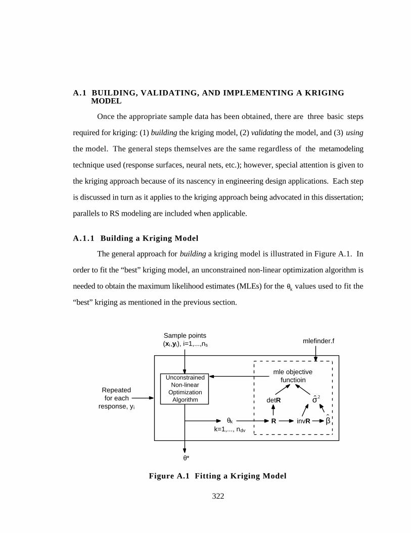
322
A.1 BUILDING, VALIDATING, AND IMPLEMENTING A KRIGINGMODEL
Once the appropriate sample data has been obtained, there are three basic steps
required for kriging: (1) building the kriging model, (2) validating the model, and (3) using
the model. The general steps themselves are the same regardless of the metamodeling
technique used (response surfaces, neural nets, etc.); however, special attention is given to
the kriging approach because of its nascency in engineering design applications. Each step
is discussed in turn as it applies to the kriging approach being advocated in this dissertation;
parallels to RS modeling are included when applicable.
A.1.1 Building a Kriging Model
The general approach for building a kriging model is illustrated in Figure A.1. In
order to fit the “best” kriging model, an unconstrained non-linear optimization algorithm is
needed to obtain the maximum likelihood estimates (MLEs) for the θk values used to fit the
“best” kriging as mentioned in the previous section.
UnconstrainedNon-linear
OptimizationAlgorithm
θk
k=1,..., ndv
mlefinder.f
R
detR
invR
mle objectivefunctioin
Sample points(xi,yi), i=1,...,ns
θ*
ˆ σ 2Repeatedfor each
response, yi
ˆ β
Figure A.1 Fitting a Kriging Model
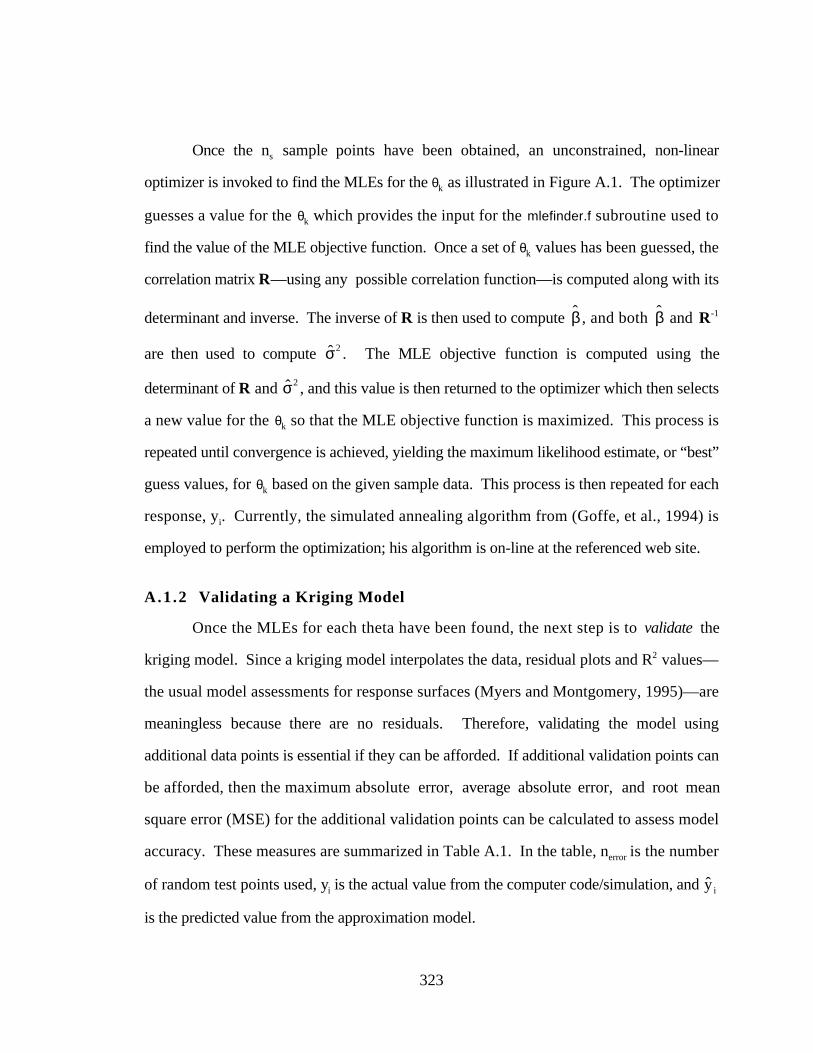
323
Once the ns sample points have been obtained, an unconstrained, non-linear
optimizer is invoked to find the MLEs for the θk as illustrated in Figure A.1. The optimizer
guesses a value for the θk which provides the input for the mlefinder.f subroutine used to
find the value of the MLE objective function. Once a set of θk values has been guessed, the
correlation matrix R—using any possible correlation function—is computed along with its
determinant and inverse. The inverse of R is then used to compute ˆ β , and both ˆ β and R-1
are then used to compute ˆ σ 2 . The MLE objective function is computed using the
determinant of R and ˆ σ 2 , and this value is then returned to the optimizer which then selects
a new value for the θk so that the MLE objective function is maximized. This process is
repeated until convergence is achieved, yielding the maximum likelihood estimate, or “best”
guess values, for θk based on the given sample data. This process is then repeated for each
response, yi. Currently, the simulated annealing algorithm from (Goffe, et al., 1994) is
employed to perform the optimization; his algorithm is on-line at the referenced web site.
A.1.2 Validating a Kriging Model
Once the MLEs for each theta have been found, the next step is to validate the
kriging model. Since a kriging model interpolates the data, residual plots and R2 values—
the usual model assessments for response surfaces (Myers and Montgomery, 1995)—are
meaningless because there are no residuals. Therefore, validating the model using
additional data points is essential if they can be afforded. If additional validation points can
be afforded, then the maximum absolute error, average absolute error, and root mean
square error (MSE) for the additional validation points can be calculated to assess model
accuracy. These measures are summarized in Table A.1. In the table, nerror is the number
of random test points used, yi is the actual value from the computer code/simulation, and ˆ y i
is the predicted value from the approximation model.
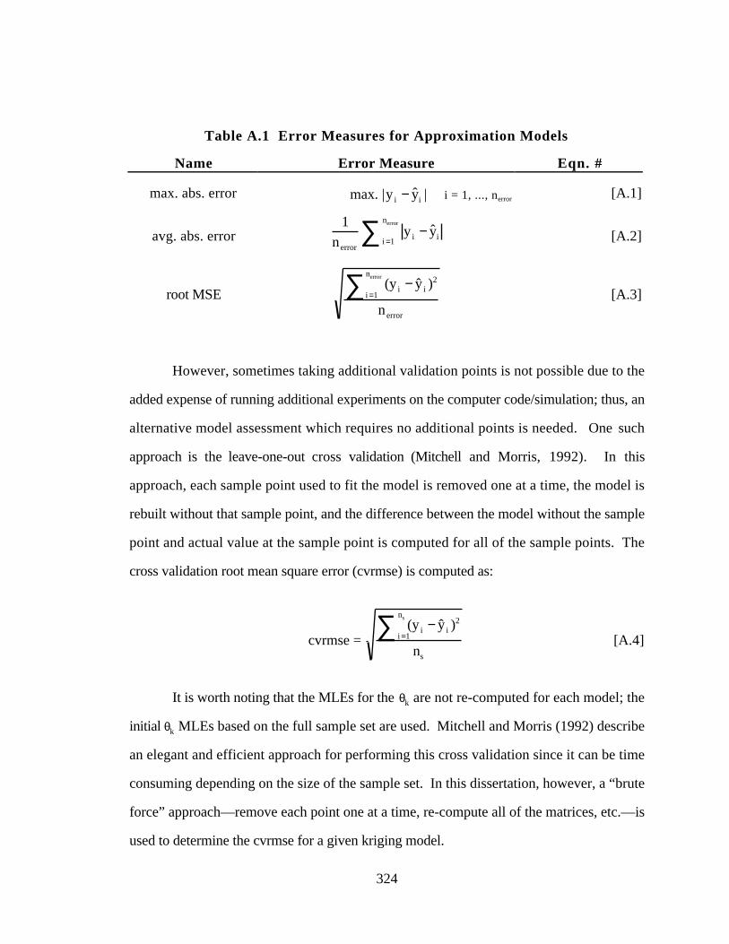
324
Table A.1 Error Measures for Approximation Models
Name Error Measure Eqn. #
max. abs. error max. |y i − ˆ y i | i = 1, ..., nerror [A.1]
avg. abs. error1
n error
y i − ˆ y ii =1
nerror∑ [A.2]
root MSE(y i − ˆ y i )
2
i =1
nerror∑n error
[A.3]
However, sometimes taking additional validation points is not possible due to the
added expense of running additional experiments on the computer code/simulation; thus, an
alternative model assessment which requires no additional points is needed. One such
approach is the leave-one-out cross validation (Mitchell and Morris, 1992). In this
approach, each sample point used to fit the model is removed one at a time, the model is
rebuilt without that sample point, and the difference between the model without the sample
point and actual value at the sample point is computed for all of the sample points. The
cross validation root mean square error (cvrmse) is computed as:
cvrmse = (y i − ˆ y i )
2
i =1
ns∑ns
[A.4]
It is worth noting that the MLEs for the θk are not re-computed for each model; the
initial θk MLEs based on the full sample set are used. Mitchell and Morris (1992) describe
an elegant and efficient approach for performing this cross validation since it can be time
consuming depending on the size of the sample set. In this dissertation, however, a “brute
force” approach—remove each point one at a time, re-compute all of the matrices, etc.—is
used to determine the cvrmse for a given kriging model.
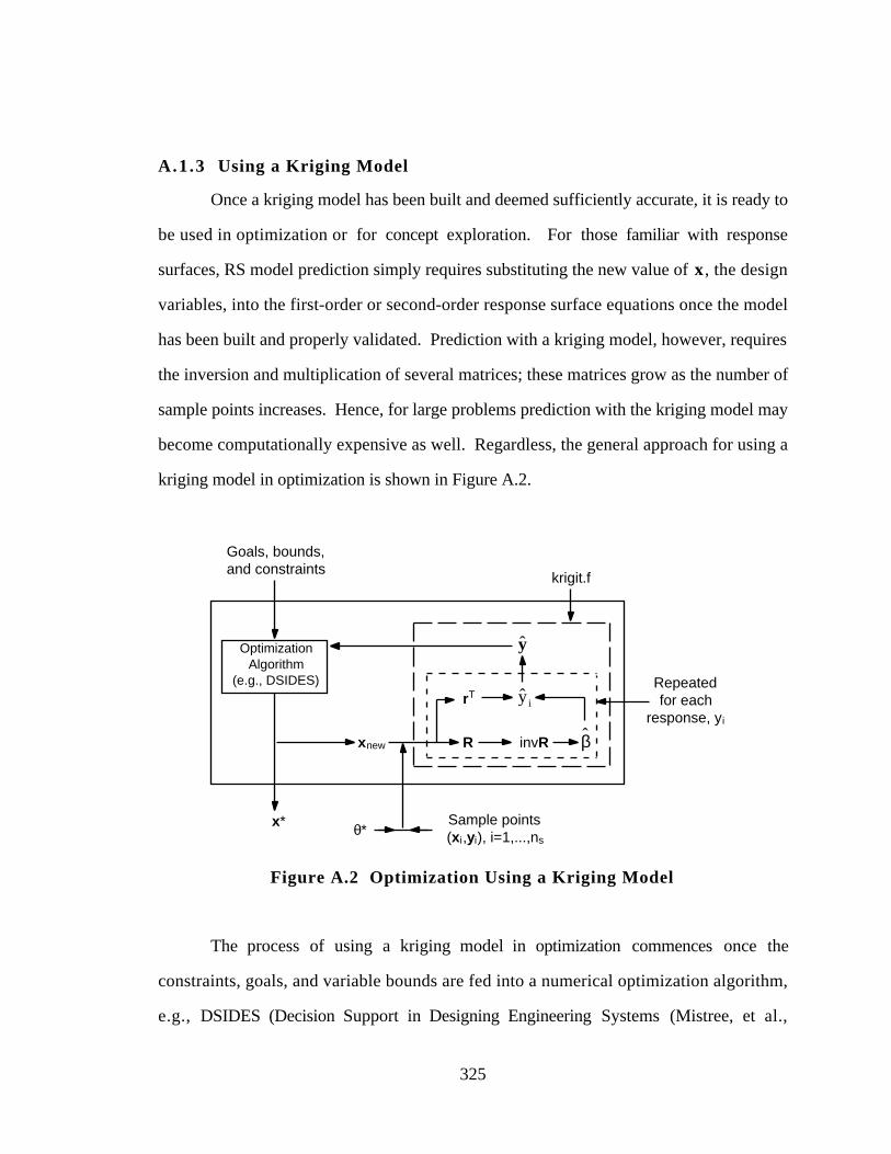
325
A.1.3 Using a Kriging Model
Once a kriging model has been built and deemed sufficiently accurate, it is ready to
be used in optimization or for concept exploration. For those familiar with response
surfaces, RS model prediction simply requires substituting the new value of x , the design
variables, into the first-order or second-order response surface equations once the model
has been built and properly validated. Prediction with a kriging model, however, requires
the inversion and multiplication of several matrices; these matrices grow as the number of
sample points increases. Hence, for large problems prediction with the kriging model may
become computationally expensive as well. Regardless, the general approach for using a
kriging model in optimization is shown in Figure A.2.
krigit.f
Sample points(xi,yi), i=1,...,ns
θ*
Repeatedfor each
response, yi
xnew
x*
rT
OptimizationAlgorithm
(e.g., DSIDES)
R invR ˆ β
ˆ y
Goals, bounds, and constraints
ˆ y i
Figure A.2 Optimization Using a Kriging Model
The process of using a kriging model in optimization commences once the
constraints, goals, and variable bounds are fed into a numerical optimization algorithm,
e.g., DSIDES (Decision Support in Designing Engineering Systems (Mistree, et al.,

326
1993)) or OptdesX (Parkinson and al., 1998). The optimization algorithm then selects a
value for the design variables: xnew. The sample points, θ* from Figure A.1, and xnew serve
as the input for the dace_eval.f subroutine used for prediction. The krigit.f algorithm is used
to compute R, the inverse of R, and then ˆ β . Meanwhile, rT is also computed, and once rT
and ˆ β are known, ˆ y i can be computed. This process is repeated for each response, and
the vector of predicted values, ˆ y , is returned to the optimizer which adjusts xnew until the
best point, x*, is found. The algorithms krigit.f and mlefinder.f are included in the next
section.
A.2 KRIGING SOURCE CODE
The kriging source code for mlefinder.f and krigit.f are included in Sections A.2.1
and A.2.2, respectively. A README file describing the intricacies of the kriging codes
and file naming conventions is included in Section A.2.3. Finally, sample parameter and
data input files and resulting output files are given in Section A.2.4.
A.2.1 The mlefinder.f Algorithm
************************************************************************ subroutine daceinter(xvector,MLE,krig)** This subroutine acts as an interface between a numerical optimizer by* providing the MLE estimate of the DACE correlation parameter 'theta'* based on the data contained in the input file opened below.** This routine (daceinter) calls the correlation subroutine (correlate)* to evaluate the correlation matrix and DACE model parameters.** Tim Simpson, 25 February 1998 / Tony Giunta, 12 May 1997************************************************************************** Input Variables:* ----------------* xvector = vector of length 'numdv' which contains theta guesses* krig = integer indicating response currently under investigation*
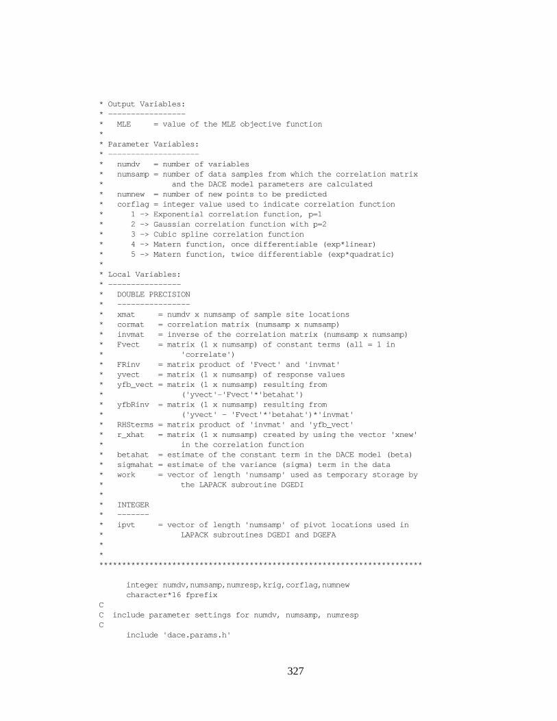
327
* Output Variables:* -----------------* MLE = value of the MLE objective function** Parameter Variables:* --------------------* numdv = number of variables* numsamp = number of data samples from which the correlation matrix* and the DACE model parameters are calculated* numnew = number of new points to be predicted* corflag = integer value used to indicate correlation function* 1 -> Exponential correlation function, p=1* 2 -> Gaussian correlation function with p=2* 3 -> Cubic spline correlation function* 4 -> Matern function, once differentiable (exp*linear)* 5 -> Matern function, twice differentiable (exp*quadratic)** Local Variables:* ----------------* DOUBLE PRECISION* ----------------* xmat = numdv x numsamp of sample site locations* cormat = correlation matrix (numsamp x numsamp)* invmat = inverse of the correlation matrix (numsamp x numsamp)* Fvect = matrix (1 x numsamp) of constant terms (all = 1 in* 'correlate')* FRinv = matrix product of 'Fvect' and 'invmat'* yvect = matrix (1 x numsamp) of response values* yfb_vect = matrix (1 x numsamp) resulting from* ('yvect'-'Fvect'*'betahat')* yfbRinv = matrix (1 x numsamp) resulting from* ('yvect' - 'Fvect'*'betahat')*'invmat'* RHSterms = matrix product of 'invmat' and 'yfb_vect'* r_xhat = matrix (1 x numsamp) created by using the vector 'xnew'* in the correlation function* betahat = estimate of the constant term in the DACE model (beta)* sigmahat = estimate of the variance (sigma) term in the data* work = vector of length 'numsamp' used as temporary storage by* the LAPACK subroutine DGEDI** INTEGER* -------* ipvt = vector of length 'numsamp' of pivot locations used in* LAPACK subroutines DGEDI and DGEFA*************************************************************************
integer numdv,numsamp,numresp,krig,corflag,numnew character*16 fprefixCC include parameter settings for numdv, numsamp, numrespC include 'dace.params.h'
328
COMMON /filename/ deckfile,fitsfile
double precision xmat(numsamp,numdv), & invmat(numsamp,numsamp),Fvect(numsamp,numdv+1),FRinv(numsamp), & yvect(numsamp),yfb_vect(numsamp),Rinvyfb(numsamp), & betahat, & MLE, work(numsamp), p,detR, & theta(numdv), xvector(numdv), resp(numsamp,numresp)
integer i,j,ipvt(numsamp),iprint character*24 deckfile,fitsfile
CC specify correlation function parameter p if necessaryC if (corflag.eq.2) then p=2.0 else if (corflag.eq.1) then p=1.0 end ifCC open necessary .dek fileC open(21,file=deckfile,status='old')CC initialize the DACE modeling parametersC do 10 i = 1,numdv theta(i) = xvector(i) 10 continueCC read in xmat and response arraysC do 100 i=1,numsamp read (21,*) (xmat(i,j),j=1,numdv),(resp(i,k),k=1,numresp) 100 continue close(21)
CC Assign response to yvect for the response of interest (specifiedC by variable 'krig'); yvect is the response for which model is beingC built using 'theta' parameters; also, initiliaze FvectC do 107 i=1,numsamp yvect(i)=resp(i,krig) Fvect(i,1)=1.0d0 107 continue
CC call subroutine to calculate the inverse of the correlation matrixC
call cormat (xmat,invmat,detR,numsamp,numdv, & work,ipvt,theta,p,corflag,iprint)

329
CC call subroutine to compute intermediate kriging equationsC
call compeqn (invmat,Fvect,yvect,FRinv,yfb_vect, & Rinvyfb,betahat,numsamp,numdv)
CC call subroutine to compute sigmahat and mle obj functionC call mleobjfcn (detR,yfb_vect,Rinvyfb,MLE,numsamp)
CC return to simulated annealing algorithm with MLE valueC return end
************************************************************************ subroutine cormat (xmat,invmat,detR,numsamp,numdv, & work,ipvt,theta,p,corflag,iprint)*** This subroutine calculates the correlation matrix and its inverse** Tim Simpson 15 February 1998 / Tony Giunta, 12 May 1997************************************************************************** Needed External Files:* ----------------------* LAPACK subroutines DGEFA and DGEDI (FORTRAN77)** Inputs:* -------* DOUBLE PRECISION:* -----------------* xmat,work,p,theta** INTEGER:* --------* numdv,numsamp,ipvt,corflag** Variables ipvt and work will be changed upon exit.** Outputs:* --------* DOUBLE PRECISION:* -----------------* invmat,detR** Local:* ------
330
* DOUBLE PRECISION:* -----------------* det(2) = dummy variable used in DGEFI subroutine* R = value of correlation function between i_th and j_th* sample points************************************************************************CC passed variablesC integer numdv,numsamp,corflag,ipvt(numsamp),iprint
double precision xmat(numsamp,numdv),invmat(numsamp,numsamp), & work(numsamp),p,theta(numdv),detRCC local variablesC integer i,j double precision det(2),RCC calculate terms in the correlation matrixC do 300 i = 1,numsamp do 305 j = i,numsamp if( i .eq. j ) then invmat(i,j) = 1.0d0 elseCC call subroutine to compute spatial correlation function for xmatC call scfxmat(R,xmat,theta,corflag,p,numdv,numsamp,i,j) invmat(i,j) = R invmat(j,i) = invmat(i,j) endif 305 continue 300 continue
if (iprint.eq.1) then do 321 i=1,numsamp 321 write(28,829) (invmat(i,j),j=1,numsamp) 829 format(5(f12.3,1x)) end ifCC calculate the inverse of the correlation matrix using dgefa and dgediC do 307 i=1,numsamp work(i)=0.0d0 ipvt(i)=0 307 continue
call dgefa(invmat, numsamp, numsamp, ipvt, info) if( info .ne. 0 ) then write(*,*)"Error in DGEFA, info = ",info stop endif
331
CC In DGEDI, last flag is: 1 (inverse only), 10 (Det only), 11 (both)C call dgedi(invmat, numsamp, numsamp, ipvt, det, work, 11) detR = det(1) * 10.0d0**det(2)C print *, 'detR=',detR, det(1), det(2)
if (iprint.eq.1) then do 320 i=1,numsamp 320 write(28,828) (invmat(i,j),j=1,numsamp) 828 format(5(f12.3,1x)) end if
return end
************************************************************************* include LAPACK routines used to find inverse of correlation matrix;* available on-line at http://www.netlib.org/************************************************************************
include 'dgefa.f' include 'dgedi.f'
************************************************************************ subroutine compeqn (invmat,Fvect,yvect,FRinv,yfb_vect, & Rinvyfb,betahat,numsamp,numdv)*** This subroutine calculates the DACE correlation matrix and* corresponding equations needed for model prediction.** Tim Simpson 15 February 1998**----------------------------------------------------------------------** Inputs:* -------* DOUBLE PRECISION:* -----------------* invmat,Fvect,yvect** Outputs:* --------* DOUBLE PRECISION:* -----------------* betahat,FRinv,Rinvyfb,yfb_vect** Local:* ------* DOUBLE PRECISION:
332
* -----------------* beta_den,beta_num************************************************************************CC passed variablesC integer numsamp,numdv
double precision betahat,invmat(numsamp,numsamp), & Fvect(numsamp,numdv+1),FRinv(numsamp), & Rinvyfb(numsamp),yvect(numsamp),yfb_vect(numsamp)CC local variablesC double precision beta_den,beta_num integer i,j
CC compute F'RinvC do 310 i=1,numsamp FRinv(i)=0.0d0 do 315 j=1,numsamp FRinv(i)=FRinv(i)+Fvect(j,1)*invmat(j,i) 315 continue 310 continue
CC compute betahat = (F'Rinv*yvect)/(F'Rinv*F)C beta_den=0.0d0 beta_num=0.0d0 do 320 i=1,numsamp beta_den=beta_den+FRinv(i)*Fvect(i,1) beta_num=beta_num+FRinv(i)*yvect(i) 320 continue betahat = beta_num / beta_den
CC compute y-f'betahatC do 330 i = 1,numsamp yfb_vect(i) = yvect(i) - betahat*Fvect(i,1) 330 continue
CC compute Rinv*(y-f'beta)C do 340 i=1,numsamp Rinvyfb(i)=0.0d0 do 345 j=1,numsamp Rinvyfb(i)=Rinvyfb(i)+invmat(i,j)*yfb_vect(j) 345 continue 340 continue
333
return end
C********************************************************************C subroutine mleobjfcn(detR,yfb_vect,Rinvyfb,MLE,numsamp)CC author: Tim Simpson date: 16 February 1998*** Inputs:* -------* DOUBLE PRECISION:* -----------------* detR,yfb_vect,Rinvyfb** INTEGER:* --------* numsamp*** Outputs:* --------* DOUBLE PRECISION:* -----------------* MLE** Local:* ------* DOUBLE PRECISION:* -----------------* sigmahat = estimated value of*C********************************************************************CC passed variablesC double precision detR,yfb_vect(numsamp),Rinvyfb(numsamp),MLE integer numsampCC local variablesC double precision sigmahat integer i
CC compute sigma_hat = (yfb_vect*Ringyfb)/numsampC sigmahat=0.0d0 do 10 i=1,numsamp sigmahat=sigmahat+yfb_vect(i)*Rinvyfb(i) 10 continue sigmahat=ABS(sigmahat)/numsamp
334
CC compute MLE objective functionC
C added first part of if loop to control MLE when near a singularityC if ((detR.lt.0.0).or.(sigmahat.lt.0.0)) then MLE = -5000. else MLE = -0.5d0*(numsamp*log(sigmahat) + log(detR)) end if
C write(6,83) sigmahat,detR,MLEC 83 format('sigmahat=',f12.4,2x,'detR=',f10.7,'obj fcn=',f12.5)
return end
C********************************************************************C subroutine scfxmat(R,xmat,theta,corflag,p,numdv,numsamp,i,j)CC author: tim simpson date: 2/11/98CC subroutine to compute correlation function for correlationC matrix; NOT to compute r_xhat.CCC Output:C -------C R = value of correlation function between two sample points,C given thetaCC Input:C ------C xmat = matrix of sample pointsC theta = array of theta valuesC i,j = i_th and j_th elements of correlation matrix for whichC correlation function is being computedC corflag = integer flag specifying correlation functionCC All variables except R are unchanged upon exitingCC********************************************************************CC passed variablesC integer i,j,corflag,numdv,numsamp double precision R,xmat(numsamp,numdv),theta(numdv),pCC local variablesC double precision sum,thetadist,dist integer k
335
if ((corflag.eq.2).or.(corflag.eq.1)) then sum=0.0d0 do 120 k = 1,numdv dist = ABS(xmat(i,k)-xmat(j,k)) sum = sum + theta(k)*((dist)**p) 120 continue R = exp( -1.0d0*sum )
else if (corflag.eq.3) then sum=1.0d0 do 130 k=1,numdv dist = ABS(xmat(i,k)-xmat(j,k)) thetadist=dist*theta(k) if (thetadist.lt.0.5) then sum=sum*(1.0-6.0*(thetadist**2)+6.0*(thetadist**3)) else if (thetadist.ge.1.0) then sum=sum*0.0 else sum=sum*(2.0*(1.0-thetadist)**3) end if 130 continueC print *, theta(1),thetadist,sum R = sum
else if (corflag.eq.4) then sum=1.0 do 140 k=1,numdv dist = ABS(xmat(i,k)-xmat(j,k)) sum = sum*(exp(-theta(k)*dist)*(1.+theta(k)*dist)) 140 continue R = sum
else if (corflag.eq.5) then sum=1.0 do 150 k=1,numdv dist = ABS(xmat(i,k)-xmat(j,k)) sum = sum*(exp(-theta(k)*dist)* & (1.+theta(k)*dist+(theta(K)**2*dist**2)/3.0)) 150 continue R = sum
end if
return end
A.2.2 The krigit.f Algorithm
************************************************************************* program krigit** This program invokes the subroutines (correlate) and (dace_eval)
336
* to evaluate the correlation matrix and predict at the value of y* at an untried x, given a correlation function and values for theta** Tim Simpson 25 February 1998 / Tony Giunta, 12 May 1997*************************************************************************** Variables:* ----------* xnew = vector of length 'numdv' where the DACE model is to be* evaluated* theta = supplied value of the correlation parameter 'theta'* ynew = vector of length 'numnew' of the DACE model response value(s)* corflag = flag variable used to specify correlation function:* 1 -> Exponential correlation function, p=1* 2 -> Gaussian correlation function, p=2* 3 -> Cubic spline correlation function* 4 -> Matern function, once differentiable (exp*linear)* 5 -> Matern function, twice differentiable (exp*quadratic)* krig = counter indicating # of response which is currently being* modeled (1 < KRIG < numresp)** Parameter Variables (to be specified by user in krig.params.h):* ----------------------------------------------------* numdv = number of variables* numsamp = number of data samples from which the correlation matrix* and the DACE model parameters are calculated* numnew = number of sample site where the unknown response value* will be calculated* numresp = number of responses for which kriging models have been* constructed** Local Variables:* ----------------* DOUBLE PRECISION* ----------------* xmat = numdv x numsamp of sample site locations* invmat = inverse of the correlation matrix (numsamp x numsamp)* Fvect = matrix (1 x numsamp) of constant terms* (all = 1 in 'correlate')* FRinv = matrix product of 'Fvect' and 'invmat'* yvect = matrix (1 x numsamp) of response values* yfb_vect = matrix (1 x numsamp) resulting from* ('yvect' - 'Fvect'*'betahat')* Rinvyfb = matrix product of 'invmat' and 'yfb_vect'* r_xhat = matrix (1 x numsamp) created by using the vector 'xnew'* in the correlation function* betahat = estimate of the constant term in the DACE model* work = vector of length 'numsamp' used as temporary storage by* the LAPACK subroutine DGEDI** INTEGER* -------* ipvt = vector of length 'numsamp' of pivot locations used in* LAPACK subroutines DGEDI and DGEFA

337
** Notes:* ------* A. All points X must be scaled [0,1]* B. Three files are needed for prediction:* 1. '*.dek' -> data file containing sample points* used to fit the model* 2. '*.fits' -> file containing theta parameters for* kriging model* 3. '*.pts' -> file containing new points at which* to predict y_hat(X)* C. Predicted y_hat are written to file 'wei.4_160.out'* D. User must specify modeling parameters in 'krig.params.h', for* instance if you want to predict 100 new points, then numnew* is changed to 100 in 'krig.params.h' file* E. Subroutines 'dgedi.f' and 'dgefa.f' must be in same directory* when compiling this code* F. Files 'krig.params.h' and 'krig.files.h' must also be in same* directory when compiling this code* G. Program must be recompiled any time changes are made to* either 'krig.files.h' or 'krig.params.h'*************************************************************************
integer numdv,numsamp,numnew,numresp,corflag character*16 fprefixCC integer parameters are specified in dace.params.h fileC include 'dace.params.h'
double precision xmat(numsamp,numdv),r_xhat(numsamp),betahat, & invmat(numsamp,numsamp),Fvect(numsamp,numdv+1),FRinv(numsamp), & Rinvyfb(numsamp),yvect(numsamp),yfb_vect(numsamp), & xnew(numnew,numdv),ynew(numnew),work(numsamp),dummy2, & Farray(numnew,numresp),thetaray(numresp,numdv), & theta(numdv),resp(numsamp,numresp),p,detR integer krig,i,j,k,ipvt(numsamp),dummy,lenstr,scfstr character*16 ftitle character*20 deckfile,fitsfile,newptfile,outfile,scfname
scfname='expgaucubma1ma2'
CC specify correlation function; make sure .fits file has correct thetasC if (corflag.eq.2) then p=2.0 else if (corflag.eq.1) then p=1.0 end ifCC open necessary .dek, .fit, .npt, and .out filesC call getlen(fprefix,lenstr)
338
ftitle=fprefix
deckfile=ftitle(1:lenstr) // '.dek' newptfile=ftitle(1:lenstr) // '.npt' scfstr=(3*(corflag-1))+1 fitsfile=ftitle(1:lenstr) // '.' // scfname(scfstr:scfstr+2) & // '.fit' outfile=ftitle(1:lenstr) // '.' // scfname(scfstr:scfstr+2) & // '.out'
open(21,file=deckfile,status='old') open(22,file=fitsfile,status='old') open(23,file=newptfile,status='old') open(27,file=outfile,status='unknown')
print * print *, deckfile,fitsfile,newptfile,outfile print *, numnew,numdv,numsamp,numrespCC initialize xmat, response, and theta arrays,C print * write(6,*) 'Reading in sample data...' do 10 i=1,numsamp 10 read (21,*) (xmat(i,j),j=1,numdv),(resp(i,k),k=1,numresp) close(21)
print * write(6,*) 'Reading in theta parameters...' do 20 i=1,numresp read(22,*) dummy,(thetaray(i,j),j=1,numdv),dummy2 write(6,1000) dummy,(thetaray(i,j),j=1,numdv) 1000 format(i2,8f9.5) 20 continue close(22)
print * write(6,*) 'Reading in new points at which to predict y_hat...' do 30 i=1,numnew read(23,*) (xnew(i,j),j=1,numdv) write(6,78) i,(xnew(i,j),j=1,numdv) 78 format(i3,2x,8(f6.4,1x)) 30 continue close(23)CC step through each response, predict new y_hat at each new pointC do 40 krig=1,numresp
write(6,1001) 1001 format(/,60('-'),/) write(6,*) 'Predicing response #',krig,' using theta paramters:'CC Assign response to yvect for the response of interest (specifiedC by variable 'krig'); yvect is the response for which model is being
339
C built using 'theta' parameters specified by 'krig'C do 50 j=1,numdv theta(j)=thetaray(krig,j) 50 continue write(6,1002) (theta(j),j=1,numdv) 1002 format(8f9.5) print * write(6,*) 'Predicted values for response #',krig do 60 i=1,numsamp yvect(i)=resp(i,krig) Fvect(i,1)=1.0d0 60 continueCC call subroutine to calculate the inverse of the correlation matrixC
call cormat (xmat,invmat,detR,numsamp,numdv, & work,ipvt,theta,p,corflag)
CC call subroutine to compute intermediate kriging equationsC
call compeqn (invmat,Fvect,yvect,FRinv,yfb_vect, & Rinvyfb,betahat,numsamp,numdv)
CC call subroutine to predict new point given correlation matrix andC the correlation parametersC
call dace_eval(xnew,xmat,r_xhat,betahat,Rinvyfb,numsamp, & numdv,numnew,theta,ynew,p,corflag)
CC store predicted values for current responseC do 80 i=1,numnew Farray(i,krig)=ynew(i) 80 continueCC compute predicted values for next response, i.e., increment 'krig'C 40 continueCC write predicted values to specified .out fileC do 90 i=1,numnew write(27,79) (Farray(i,krig),krig=1,numresp) 79 format(10(f13.5,1x)) 90 continue close(27)
print *
340
write(6,*) 'All response values written to specified .out file'
stop end
************************************************************************ subroutine getlen(string,lenstr)*** This subroutine is used to determine the actual length of the* filename prefix specified by the user in 'krig.params.h'.** With this known, the .dek, .fit, .npt, and .out suffixes are* concatenated onto the prefix, and the files are opened.** Author: Tim Simpson, 2/15/98** From: Koffman and Friedman, Fortran (5th ed.), Addison-Wesley,* New York, pp. 537-538.************************************************************************* character*1 blank character*16 string parameter (blank=' ') integer next do 10 next = LEN(string), 1, -1 if (string(next:next).ne.blank) then lenstr=next return end if 10 continue lenstr=0 if (lenstr.eq.0) then write(6,*) 'You have not specified a file name prefix' stop end if return end
************************************************************************ subroutine cormat (xmat,invmat,detR,numsamp,numdv, & work,ipvt,theta,p,corflag)*** This subroutine calculates the correlation matrix and its inverse** Tim Simpson 15 February 1998 / Tony Giunta, 12 May 1997************************************************************************** Needed External Files:* ----------------------
341
* LAPACK subroutines DGEFA and DGEDI (FORTRAN77)** Inputs:* -------* DOUBLE PRECISION:* -----------------* xmat,work,p,theta** INTEGER:* --------* numdv,numsamp,ipvt,corflag** Variables ipvt and work will be changed upon exit.** Outputs:* --------* DOUBLE PRECISION:* -----------------* invmat,detR (used in mle*.f but not dace*.f -> done to maintain* consistency between cormat routine for two codes)** Local:* ------* DOUBLE PRECISION:* -----------------* det(2) = dummy variable used in DGEFI subroutine* R = value of correlation function between i_th and j_th* sample points************************************************************************CC passed variablesC integer numdv,numsamp,corflag,ipvt(numsamp)
double precision xmat(numsamp,numdv),invmat(numsamp,numsamp), & work(numsamp),p,theta(numdv),detRCC local variablesC integer i,j double precision det(2),RCC calculate terms in the correlation matrixC do 300 i = 1,numsamp do 305 j = i,numsamp if( i .eq. j ) then invmat(i,j) = 1.0d0 elseCC call subroutine to compute spatial correlation function for xmatC call scfxmat(R,xmat,theta,corflag,p,numdv,numsamp,i,j) invmat(i,j) = R
342
invmat(j,i) = invmat(i,j) endif 305 continue 300 continueCC calculate the inverse of the correlation matrix using dgefa and dgefiC do 307 i=1,numsamp work(i)=0.0d0 ipvt(i)=0 307 continue
call dgefa(invmat, numsamp, numsamp, ipvt, info) if( info .ne. 0 ) then write(*,*)"Error in DGEFA, info = ",info stop endifCC In DGEDI, last flag is: 1 (inverse only), 10 (Det only), 11 (both)C call dgedi(invmat, numsamp, numsamp, ipvt, det, work, 11) detR=det(1)*10.0d0**det(2)
return end
************************************************************************* include LINPACK routines used to find inverse of correlation matrix************************************************************************
include 'dgefa.f' include 'dgedi.f'
************************************************************************ subroutine compeqn (invmat,Fvect,yvect,FRinv,yfb_vect, & Rinvyfb,betahat,numsamp,numdv)*** This subroutine calculates the DACE correlation matrix and* corresponding equations needed for model prediction.** Tim Simpson 15 February 1998**----------------------------------------------------------------------** Inputs:* -------* DOUBLE PRECISION:* -----------------* invmat,Fvect,yvect*
343
* Outputs:* --------* DOUBLE PRECISION:* -----------------* betahat,FRinv,Rinvyfb,yfb_vect** Local:* ------* DOUBLE PRECISION:* -----------------************************************************************************CC passed variablesC integer numsamp,numdv
double precision betahat,invmat(numsamp,numsamp), & Fvect(numsamp,numdv+1),FRinv(numsamp), & Rinvyfb(numsamp),yvect(numsamp),yfb_vect(numsamp)CC local variablesC double precision beta_den,beta_num
integer i,j
CC compute F'RinvC do 310 i=1,numsamp FRinv(i)=0.0d0 do 315 j=1,numsamp FRinv(i)=FRinv(i)+Fvect(j,1)*invmat(j,i) 315 continue 310 continueCC compute betahat = (F'Rinv*yvect)/(F'Rinv*F)C beta_den=0.0d0 beta_num=0.0d0 do 320 i=1,numsamp beta_den=beta_den+FRinv(i)*Fvect(i,1) beta_num=beta_num+FRinv(i)*yvect(i) 320 continue betahat = beta_num / beta_den print *, 'betahat=',betahatCC compute y-f'betahatC do 330 i = 1,numsamp yfb_vect(i) = yvect(i) - betahat*Fvect(i,1) 330 continueCC compute Rinv*(y-f'beta)

344
C do 340 i=1,numsamp Rinvyfb(i)=0.0d0 do 345 j=1,numsamp Rinvyfb(i)=Rinvyfb(i)+invmat(i,j)*yfb_vect(j) 345 continue 340 continue
return end
************************************************************************ subroutine dace_eval(xnew,xmat,r_xhat,betahat,Rinvyfb, & numsamp,numdv,numnew,theta,ynew,p,corflag)*** Use DACE interpolating model to predict response values at unsampled* locations** Tony Giunta, 12 May 1997/Tim Simpson 12 February 1998************************************************************************** Inputs:* -------* xnew* xmat* r_xhat* betahat* Rinvyfb* numsamp* numdv* theta** Outputs:* --------* ynew** Local Variables:* ----------------* sum = temporary variable used for calculating the terms in the* vector 'r_xhat'* yeval = scalar value resulting from matrix multiplication of* 'r_xhat' * 'Rinvyfb'************************************************************************** double precision xnew(numnew,numdv),r_xhat(numsamp), & xmat(numsamp,numdv),Rinvyfb(numsamp),betahat, & theta(numdv),ynew(numnew),yeval,p,R integer i,j,k,numdv,numsamp,numnew,corflagC
345
C calculate the vector r(x)C do 200 i = 1,numnew do 210 j = 1,numsamp call scfxnew(R,xnew,xmat,theta,corflag,p,numdv,numsamp, & numnew,i,j)CC equate r_xhat to correlation between ith xnew point and jth sample pointC r_xhat(j)=R 210 continueCC calculate the estimate of Y, i.e., Y_hat(x)C yeval = 0.0d0 do 220 k=1,numsamp 220 yeval=yeval+r_xhat(k)*Rinvyfb(k) ynew(i) = yeval + betahat print '(f20.5)', ynew(i)
CC repeat for next xnewC 200 continue
return end
C********************************************************************C subroutine scfxmat(R,xmat,theta,corflag,p,numdv,numsamp,i,j)CC Author: Tim Simpson Date: 2/11/98CC subroutine to compute spatial correlation function (scf) forC correlation matrix; NOT to compute scf for r_xhat.CC Output:C -------C R = value of correlation function between two sample points,C given thetaCC Input:C ------C xmat = matrix of sample pointsC theta = array of theta valuesC i,j = i_th and j_th elements of correlation matrix for whichC correlation function is being computedC corflag = integer flag specifying correlation function:CC All variables except R are unchanged upon exitingCC********************************************************************CC passed variables
346
C integer i,j,corflag,numdv,numsamp double precision R,xmat(numsamp,numdv),theta(numdv),pCC local variablesC double precision sum,thetadist,dist integer k
if ((corflag.eq.2).or.(corflag.eq.1)) then sum=0.0d0 do 120 k = 1,numdv dist = ABS(xmat(i,k)-xmat(j,k)) sum = sum + theta(k)*((dist)**p) 120 continue R = exp( -1.0d0*sum )
else if (corflag.eq.3) then sum=1.0d0 do 130 k=1,numdv dist = ABS(xmat(i,k)-xmat(j,k)) thetadist=dist*theta(k) if (thetadist.lt.0.5) then sum=sum*(1.0-6.0*(thetadist**2)+6.0*(thetadist**3)) else if (thetadist.ge.1.0) then sum=sum*0.0 else sum=sum*(2.0*(1.0-thetadist)**3) end if 130 continue R = sum
else if (corflag.eq.4) then sum=1.0 do 140 k=1,numdv dist = ABS(xmat(i,k)-xmat(j,k)) sum = sum*(exp(-theta(k)*dist)*(1.+theta(k)*dist)) 140 continue R = sum
else if (corflag.eq.5) then sum=1.0 do 150 k=1,numdv dist = ABS(xmat(i,k)-xmat(j,k)) thetadist=dist*theta(k) sum = sum*(exp(-thetadist)* & (1.+thetadist+(thetadist**2)/3.0)) 150 continue R = sum
end if
return end
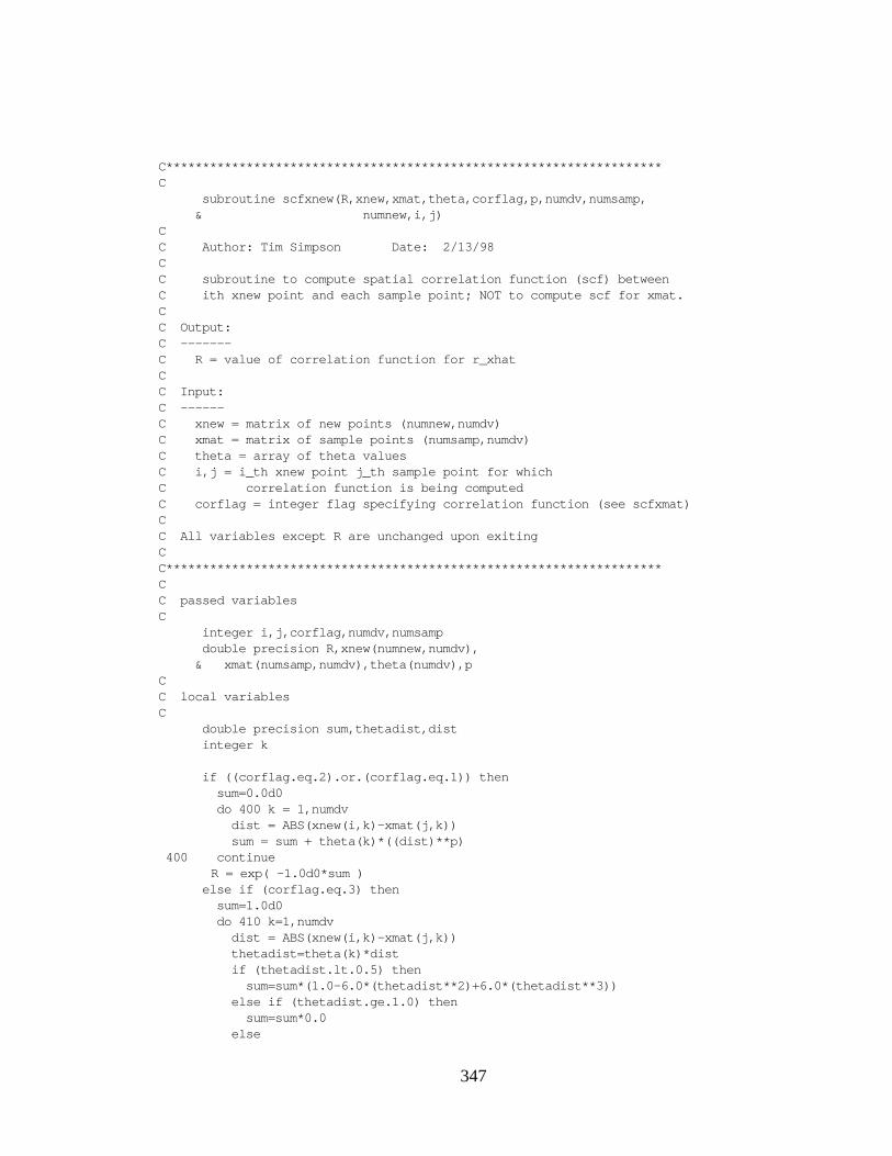
347
C********************************************************************C subroutine scfxnew(R,xnew,xmat,theta,corflag,p,numdv,numsamp, & numnew,i,j)CC Author: Tim Simpson Date: 2/13/98CC subroutine to compute spatial correlation function (scf) betweenC ith xnew point and each sample point; NOT to compute scf for xmat.CC Output:C -------C R = value of correlation function for r_xhatCC Input:C ------C xnew = matrix of new points (numnew,numdv)C xmat = matrix of sample points (numsamp,numdv)C theta = array of theta valuesC i,j = i_th xnew point j_th sample point for whichC correlation function is being computedC corflag = integer flag specifying correlation function (see scfxmat)CC All variables except R are unchanged upon exitingCC********************************************************************CC passed variablesC integer i,j,corflag,numdv,numsamp double precision R,xnew(numnew,numdv), & xmat(numsamp,numdv),theta(numdv),pCC local variablesC double precision sum,thetadist,dist integer k
if ((corflag.eq.2).or.(corflag.eq.1)) then sum=0.0d0 do 400 k = 1,numdv dist = ABS(xnew(i,k)-xmat(j,k)) sum = sum + theta(k)*((dist)**p) 400 continue R = exp( -1.0d0*sum ) else if (corflag.eq.3) then sum=1.0d0 do 410 k=1,numdv dist = ABS(xnew(i,k)-xmat(j,k)) thetadist=theta(k)*dist if (thetadist.lt.0.5) then sum=sum*(1.0-6.0*(thetadist**2)+6.0*(thetadist**3)) else if (thetadist.ge.1.0) then sum=sum*0.0 else
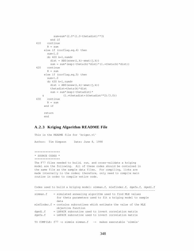
348
sum=sum*(2.0*(1.0-thetadist)**3) end if 410 continue R = sum else if (corflag.eq.4) then sum=1.0 do 420 k=1,numdv dist = ABS(xnew(i,k)-xmat(j,k)) sum = sum*(exp(-theta(k)*dist)*(1.+theta(k)*dist)) 420 continue R = sum else if (corflag.eq.5) then sum=1.0 do 430 k=1,numdv dist = ABS(xnew(i,k)-xmat(j,k)) thetadist=theta(k)*dist sum = sum*(exp(-thetadist)* & (1.+thetadist+(thetadist**2)/3.0)) 430 continue R = sum end if
return end
A.2.3 Kriging Algorithm README File
This is the README file for 'kriger.v1'
Author: Tim Simpson Date: June 8, 1998
***************** SOURCE CODES *****************The F77 files needed to build, run, and cross-validate a krigingmodel are the following. All of these codes should be contained inthe same file as the sample data files. For compiling, links aremade internally to the codes; therefore, only need to compile mainroutine in order to compile entire code.
Codes used to build a kriging model: simman.f, mlefinder.f, dgefa.f, dgedi.f----------------------------------------------------------------------------simman.f = simulated annealing algorithm used to find MLE values for theta parameters used to fit a kriging model to sample datamlefinder.f = contains subroutines which estimate the value of the MLE objective functiondgedi.f = LAPACK subroutine used to invert correlation matrixdgefa.f = LAPACK subroutine used to invert correlation matrix
TO COMPILE: f77 -o simmle simman.f -> makes executable 'simmle'
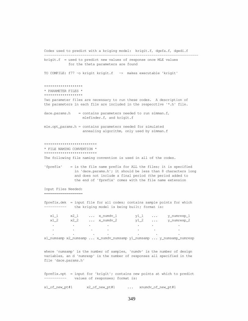
349
Codes used to predict with a kriging model: krigit.f, dgefa.f, dgedi.f----------------------------------------------------------------------------krigit.f = used to predict new values of response once MLE values for the theta parameters are found
TO COMPILE: f77 -o krigit krigit.f -> makes executable 'krigit'
******************** PARAMETER FILES ********************Two parameter files are necessary to run these codes. A description ofthe parameters in each file are included in the respecctive '*.h' file.
dace.params.h = contains parameters needed to run simman.f, mlefinder.f, and krigit.f
mle.opt_params.h = contains parameters needed for simulated annealing algorithm, only used by simman.f
*************************** FILE NAMING CONVENTION ***************************The following file naming convention is used in all of the codes.
'fprefix' = is the file name prefix for ALL the files; it is specified in 'dace.params.h'; it should be less than 8 characters long and does not include a final period (the period added to the end of 'fprefix' comes with the file name extension
Input Files Needed:===================
fprefix.dek = input file for all codes; contains sample points for which----------- the kriging model is being built; format is:
x1_1 x2_1 ... x_numdv_1 y1_1 ... y_numresp_1 x1_2 x2_2 ... x_numdv_2 y1_2 ... y_numresp_2 . . . . . . . . . . . . . . . . . . . . .x1_numsamp x2_numsamp ... x_numdv_numsamp y1_numsamp ... y_numsamp_numresp
where 'numsamp' is the number of samples, 'numdv' is the number of designvariables, an d 'numresp' is the number of responses all specified in thefile 'dace.params.h'
fprefix.npt = input for 'krigit'; contains new points at which to predict----------- values of responses; format is:
x1_of_new_pt#1 x2_of_new_pt#1 ... xnumdv_of_new_pt#1

350
x1_of_new_pt#2 x2_of_new_pt#2 ... xnumdv_of_new_pt#2 . . . . . . . . . . . .x1_of_new_pt#numnew x2_of_new_pt#numnew ... xnumdv_of_new_pt#numnew
where 'numnew' is the number of new points as specified in 'dace.params.h'
Output Files Generated:=======================
fprefix.*.fit = output from 'simmle'; contains the MLE values for theta------------- and also the corresponding MLE objective function value; format is:
1 MLE_theta_x1 MLE_theta_x2 ... MLE_theta_x_numdv MLE_obj_fcn_value 2 MLE_theta_x1 MLE_theta_x2 ... MLE_theta_x_numdv MLE_obj_fcn_value . . . . . . . . . . . . . . . . . .numresp MLE_theta_x1 MLE_theta_x2 ... MLE_theta_x_numdv MLE_obj_fcn_value
where 'numresp' is the number of responses and 'numdv' is the number ofdesign variables as specified in 'dace.params.h'
The '*' in 'fprefix.*.fit' is a three letter abbreviation for thecorrelation function used to fit the model:
exp = exponential correlation function gau = gaussian correlation function cub = cubic correlation function ma1 = linear matern function (linear times exponential) ma2 = quadratic matern function (quadratic times exponential)
This three letter abbreviation is automatically derived from 'corflag'
fprefix.*.out = output from 'krigit'; contains the predicted values of------------- the response at each new point; format is:
y1_new_pt1 y2_new_pt1 ... y_numresp_new_pt1 . . . . . . . . . . . .y1_new_pt_numnew y2_new_pt_numnew ... y_numresp_new_pt_numnew
where 'numresp' is the number of responses and 'numnew' is the number ofpoints at which y is predicted; both are specified in 'dace.params.h'

351
****************** EXAMPLE FILES ******************
An example two-bar truss problem is included to test to see if thecode is working properly. The problem has 2 design variables and3 responses; the file prefix is '2bar'.
The sample data file is '2bar.dek' and the 'dace.params.h' file hasbeen renamed '2bar.h' for ease of association with the example. Thenew point file is '2bar.npt' and contains 11 points at which topredict new values of the responses.
To make sure the code is working properly:
1. copy '2bar.h' to 'dace.params.h' : %user>cp 2bar.h dace.params.h
2. complie 'simmle' : %user>f77 -o simmle simman.f
3. execute 'simmle' to find MLEs : %user>simmle
4. after 'simmle' is complete, check contents of '2bar.gau.fit' and compare to '2bar.gau.fit%'. Here, the correlation function used in '2bar.h' is corflag=2, the Gaussian correlation function
5. compile 'krigit' : %user>f77 -o krigit krigit.f
6. execute 'krigit' to predict new y : %user>krigit
7. after 'krigit' is complete, check contents of '2bar.out' and compare to '2bar.gau.out%'.
*********************************** SOME FINAL NOTES AND POINTERS ***********************************
1. All x (design variables) in *.dek must be scaled to [0,1].
2. As with the 2bar example, it helps to maintain a '*.h' file for each problem and then just copy that file to 'dace.params.h' when needed, rather than recreat 'dace.params.h' each time.
3. The optimization parameters in the 'mle.opt_params.h' file are rather conservatively set in the enclosed example. It is left up to the user to find settings for EPS, RT, NS, and NT which yield sufficiently good results yet do not require long optimization runs. The current settings work well for problems with as many as 10 variables and 121 sample points. Please see the comments in the introduction to the 'simman.f' file to learn more about these parameters.
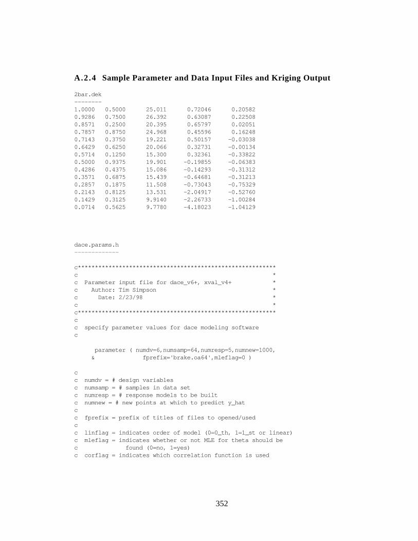
352
A.2.4 Sample Parameter and Data Input Files and Kriging Output
2bar.dek--------1.0000 0.5000 25.011 0.72046 0.205820.9286 0.7500 26.392 0.63087 0.225080.8571 0.2500 20.395 0.65797 0.020510.7857 0.8750 24.968 0.45596 0.162480.7143 0.3750 19.221 0.50157 -0.030380.6429 0.6250 20.066 0.32731 -0.001340.5714 0.1250 15.300 0.32361 -0.338220.5000 0.9375 19.901 -0.19855 -0.063830.4286 0.4375 15.086 -0.14293 -0.313120.3571 0.6875 15.439 -0.64681 -0.312130.2857 0.1875 11.508 -0.73043 -0.753290.2143 0.8125 13.531 -2.04917 -0.527600.1429 0.3125 9.9140 -2.26733 -1.002840.0714 0.5625 9.7780 -4.18023 -1.04129
dace.params.h-------------
c**********************************************************c *c Parameter input file for dace_v6+, xval_v4+ *c Author: Tim Simpson *c Date: 2/23/98 *c *c**********************************************************cc specify parameter values for dace modeling softwarec
parameter ( numdv=6,numsamp=64,numresp=5,numnew=1000, & fprefix='brake.oa64',mleflag=0 )
cc numdv = # design variablesc numsamp = # samples in data setc numresp = # response models to be builtc numnew = # new points at which to predict y_hatcc fprefix = prefix of titles of files to opened/usedcc linflag = indicates order of model (0=0_th, 1=1_st or linear)c mleflag = indicates whether or not MLE for theta should bec found (0=no, 1=yes)c corflag = indicates which correlation function is used
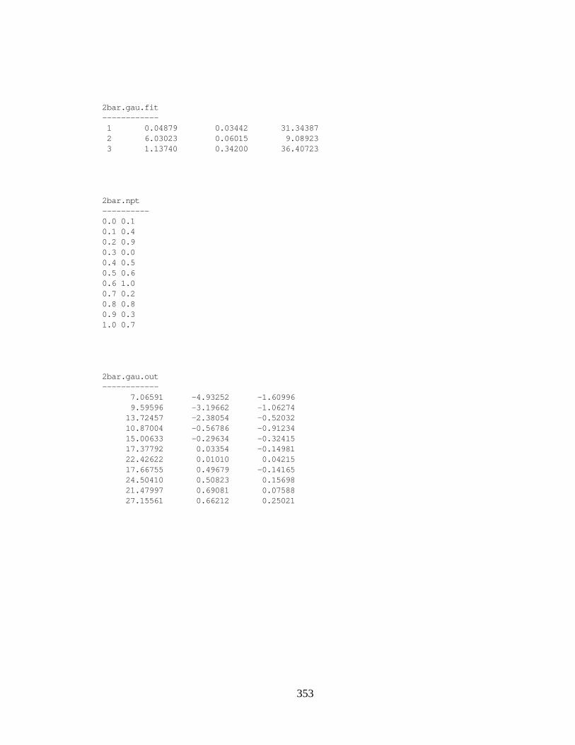
353
2bar.gau.fit------------ 1 0.04879 0.03442 31.34387 2 6.03023 0.06015 9.08923 3 1.13740 0.34200 36.40723
2bar.npt----------0.0 0.10.1 0.40.2 0.90.3 0.00.4 0.50.5 0.60.6 1.00.7 0.20.8 0.80.9 0.31.0 0.7
2bar.gau.out------------ 7.06591 -4.93252 -1.60996 9.59596 -3.19662 -1.06274 13.72457 -2.38054 -0.52032 10.87004 -0.56786 -0.91234 15.00633 -0.29634 -0.32415 17.37792 0.03354 -0.14981 22.42622 0.01010 0.04215 17.66755 0.49679 -0.14165 24.50410 0.50823 0.15698 21.47997 0.69081 0.07588 27.15561 0.66212 0.25021
354
B. APPENDIX B
EXPERIMENTAL DESIGN DESCRIPTIONS
Detailed descriptions of the experimental designs used in the kriging/DOE study in
Chapter 5 are presented in this appendix. As introduced in Section 2.4.3, two types of
classical experimental designs are considered in this work: central composite designs and
Box-Behnken designs. They are described in Sections B.1.1 and B.1.2, respectively. In
addition to these two types of classical designs, nine types of space filling designs are
studied in Chapter 5, testing Hypothesis 3 and the utility of space filling designs for
deterministic computer experiments. Of these nine space filling designs, eight are
described in this appendix in Sections B.2.1 through B.2.8. These designs include the
following: random Latin hypercubes, random orthogonal arrays, IMSE optimal Latin
hypercubes, maximin Latin hypercubes, orthogonal-array based Latin hypercubes, uniform
designs, orthogonal Latin hypercubes, and Hammersley sequence designs. The ninth
space filling experimental design—the minimax Latin hypercube which is unique to this
dissertation—is described separately in Appendix C.
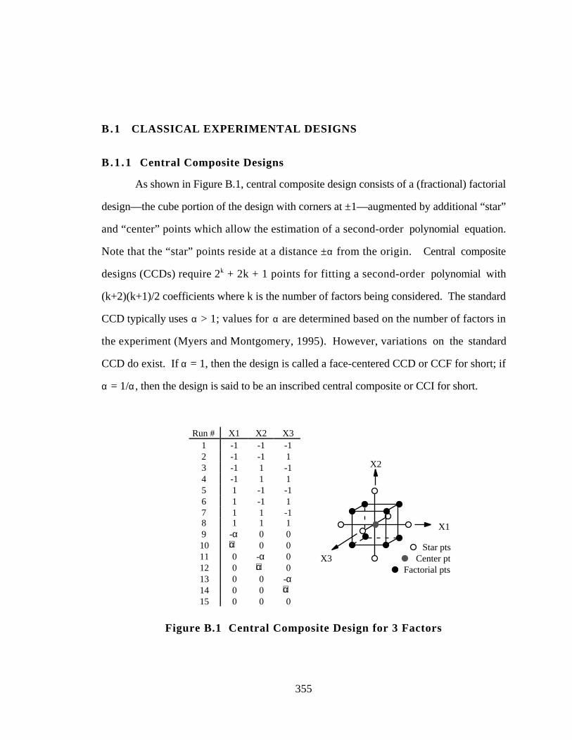
355
B.1 CLASSICAL EXPERIMENTAL DESIGNS
B.1 .1 Central Composite Designs
As shown in Figure B.1, central composite design consists of a (fractional) factorial
design—the cube portion of the design with corners at ±1—augmented by additional “star”
and “center” points which allow the estimation of a second-order polynomial equation.
Note that the “star” points reside at a distance ±α from the origin. Central composite
designs (CCDs) require 2k + 2k + 1 points for fitting a second-order polynomial with
(k+2)(k+1)/2 coefficients where k is the number of factors being considered. The standard
CCD typically uses α > 1; values for α are determined based on the number of factors in
the experiment (Myers and Montgomery, 1995). However, variations on the standard
CCD do exist. If α = 1, then the design is called a face-centered CCD or CCF for short; if
α = 1/α, then the design is said to be an inscribed central composite or CCI for short.
Run # X1 X2 X31 -1 -1 -12 -1 -1 13 -1 1 -14 -1 1 15 1 -1 -16 1 -1 17 1 1 -18 1 1 19 -α 0 010 +α 0 011 0 -α 012 0 +α 013 0 0 -α14 0 0 +α15 0 0 0
X1
X2
X3Star pts
Center ptFactorial pts
Figure B.1 Central Composite Design for 3 Factors
356
Central composite designs have many desirable features (e.g., rotatable,
orthogonal, blockable, etc.) for fitting non-deterministic data with random error (cf.,Myers
and Montgomery, 1995); however, as Sacks, et al. (1989) point out, “because
deterministic computer experiments lack random error...the classical notions of
experimental blocking, replication, and randomization are irrelevant.” Regardless, central
composite designs are employed in this work as a basis for comparison since they are
quickly becoming, or maybe already are, the standard approach for fitting second-order
response surface models in engineering computer applications (cf., Simpson, et al., 1997).
Specifically, CCF designs, a scaled CCD (where α = 1 and the factorial points lie at ±1/α),
a CCI, and a combination CCF+CCD and a combination CCF+CCI are employed in this
work. The reader is again referred to (Simpson, et al., 1997) for a review of several
studies comparing CCDs and other types of classical experimental designs.
B.1 .2 Box-Behnken Designs
Box-Behnken (BB) designs (Box and Behnken, 1960; Myers and Montgomery, 1995) are
a family of efficient three-level designs for fitting second-order response surfaces that are
formed by combining 2k factorial and incomplete block designs. They are an important
alternative to central composite designs because they require only three levels of each
factor; however, Myers and Montgomery (1995) warn that BB designs should not be used
when accurate predictions at the extremes (i.e., the corners of the hypercube) are important.
They recommend using a face-centered CCD in such cases. An inspection of the three
factor Box-Behnken design shown in Figure B.2 illustrates the lack of points near the
corners of the cube and thus the poor prediction capability of the Box-Behnken designs in
this region.
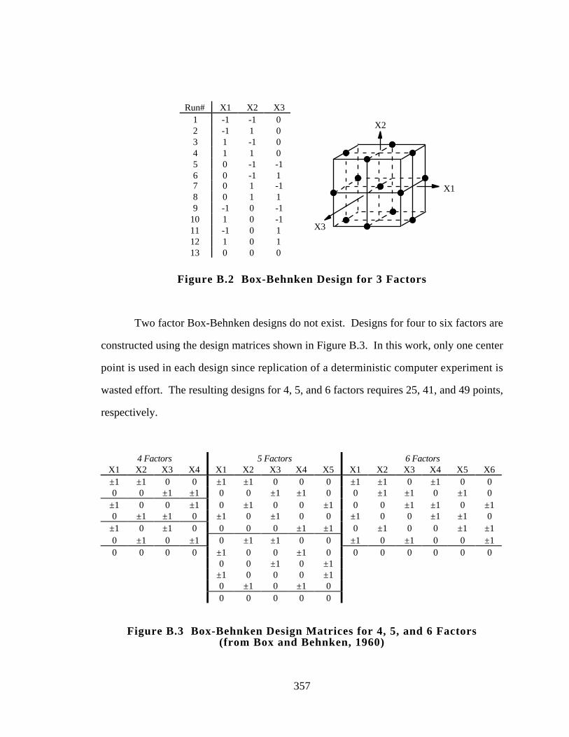
357
Run# X1 X2 X31 -1 -1 02 -1 1 03 1 -1 04 1 1 05 0 -1 -16 0 -1 17 0 1 -18 0 1 19 -1 0 -1
10 1 0 -111 -1 0 112 1 0 113 0 0 0
X1
X2
X3
Figure B.2 Box-Behnken Design for 3 Factors
Two factor Box-Behnken designs do not exist. Designs for four to six factors are
constructed using the design matrices shown in Figure B.3. In this work, only one center
point is used in each design since replication of a deterministic computer experiment is
wasted effort. The resulting designs for 4, 5, and 6 factors requires 25, 41, and 49 points,
respectively.
4 Factors 5 Factors 6 FactorsX1 X2 X3 X4 X1 X2 X3 X4 X5 X1 X2 X3 X4 X5 X6±1 ±1 0 0 ±1 ±1 0 0 0 ±1 ±1 0 ±1 0 00 0 ±1 ±1 0 0 ±1 ±1 0 0 ±1 ±1 0 ±1 0
±1 0 0 ±1 0 ±1 0 0 ±1 0 0 ±1 ±1 0 ±10 ±1 ±1 0 ±1 0 ±1 0 0 ±1 0 0 ±1 ±1 0
±1 0 ±1 0 0 0 0 ±1 ±1 0 ±1 0 0 ±1 ±10 ±1 0 ±1 0 ±1 ±1 0 0 ±1 0 ±1 0 0 ±10 0 0 0 ±1 0 0 ±1 0 0 0 0 0 0 0
0 0 ±1 0 ±1±1 0 0 0 ±10 ±1 0 ±1 00 0 0 0 0
Figure B.3 Box-Behnken Design Matrices for 4, 5, and 6 Factors(from Box and Behnken, 1960)
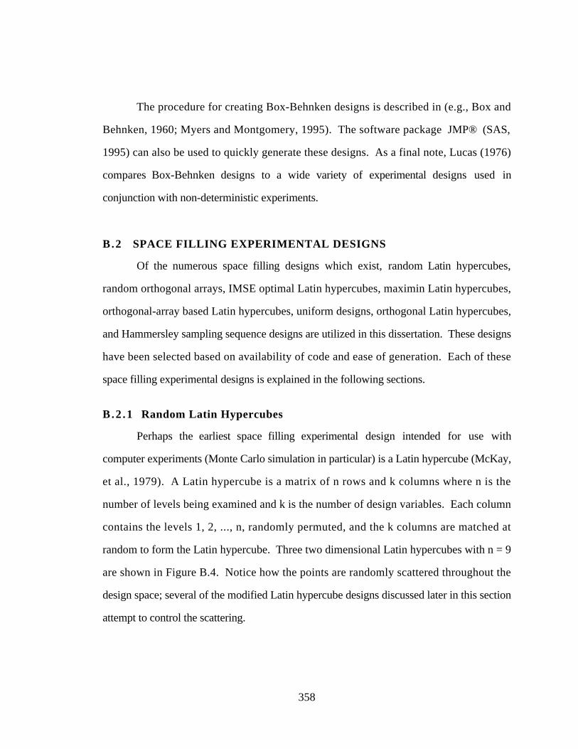
358
The procedure for creating Box-Behnken designs is described in (e.g., Box and
Behnken, 1960; Myers and Montgomery, 1995). The software package JMP® (SAS,
1995) can also be used to quickly generate these designs. As a final note, Lucas (1976)
compares Box-Behnken designs to a wide variety of experimental designs used in
conjunction with non-deterministic experiments.
B.2 SPACE FILLING EXPERIMENTAL DESIGNS
Of the numerous space filling designs which exist, random Latin hypercubes,
random orthogonal arrays, IMSE optimal Latin hypercubes, maximin Latin hypercubes,
orthogonal-array based Latin hypercubes, uniform designs, orthogonal Latin hypercubes,
and Hammersley sampling sequence designs are utilized in this dissertation. These designs
have been selected based on availability of code and ease of generation. Each of these
space filling experimental designs is explained in the following sections.
B.2 .1 Random Latin Hypercubes
Perhaps the earliest space filling experimental design intended for use with
computer experiments (Monte Carlo simulation in particular) is a Latin hypercube (McKay,
et al., 1979). A Latin hypercube is a matrix of n rows and k columns where n is the
number of levels being examined and k is the number of design variables. Each column
contains the levels 1, 2, ..., n, randomly permuted, and the k columns are matched at
random to form the Latin hypercube. Three two dimensional Latin hypercubes with n = 9
are shown in Figure B.4. Notice how the points are randomly scattered throughout the
design space; several of the modified Latin hypercube designs discussed later in this section
attempt to control the scattering.
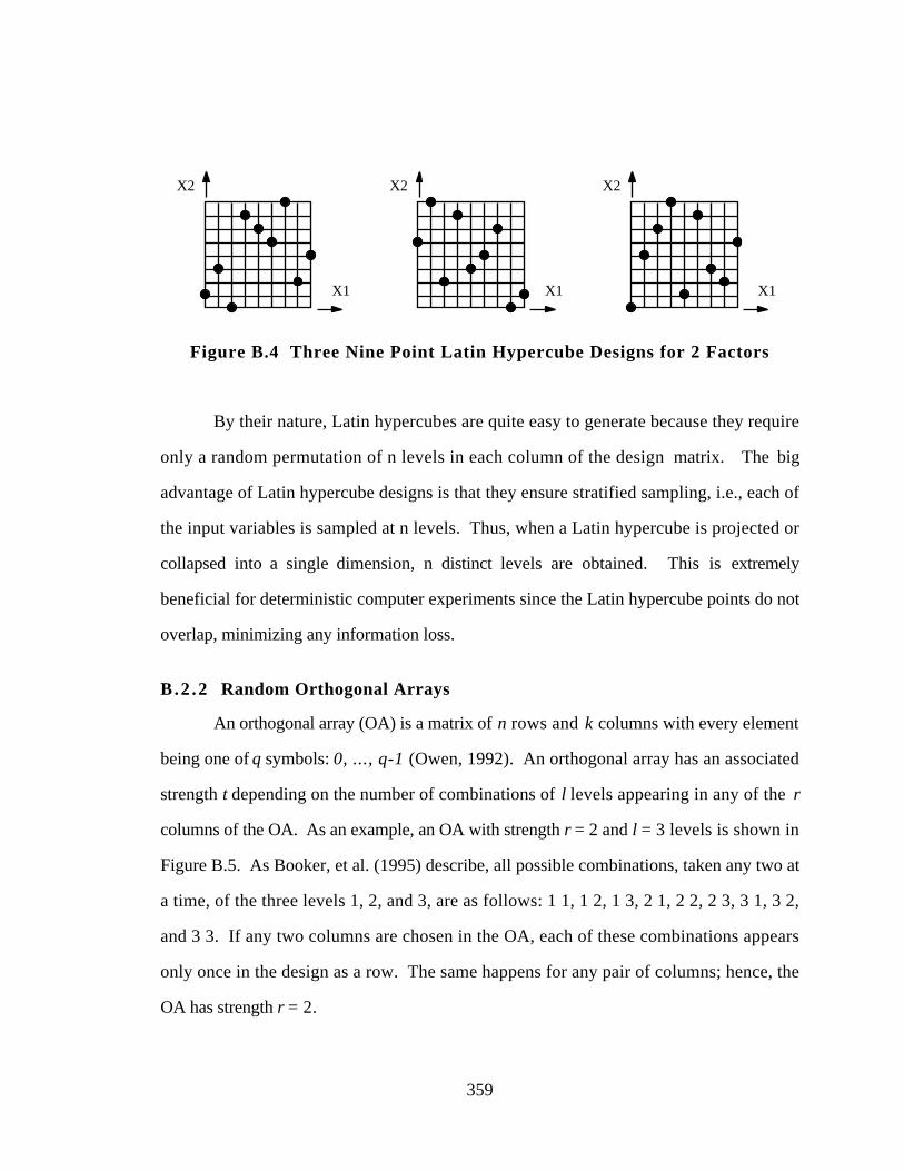
359
X1
X2
X1
X2
X1
X2
Figure B.4 Three Nine Point Latin Hypercube Designs for 2 Factors
By their nature, Latin hypercubes are quite easy to generate because they require
only a random permutation of n levels in each column of the design matrix. The big
advantage of Latin hypercube designs is that they ensure stratified sampling, i.e., each of
the input variables is sampled at n levels. Thus, when a Latin hypercube is projected or
collapsed into a single dimension, n distinct levels are obtained. This is extremely
beneficial for deterministic computer experiments since the Latin hypercube points do not
overlap, minimizing any information loss.
B.2 .2 Random Orthogonal Arrays
An orthogonal array (OA) is a matrix of n rows and k columns with every element
being one of q symbols: 0, ..., q-1 (Owen, 1992). An orthogonal array has an associated
strength t depending on the number of combinations of l levels appearing in any of the r
columns of the OA. As an example, an OA with strength r = 2 and l = 3 levels is shown in
Figure B.5. As Booker, et al. (1995) describe, all possible combinations, taken any two at
a time, of the three levels 1, 2, and 3, are as follows: 1 1, 1 2, 1 3, 2 1, 2 2, 2 3, 3 1, 3 2,
and 3 3. If any two columns are chosen in the OA, each of these combinations appears
only once in the design as a row. The same happens for any pair of columns; hence, the
OA has strength r = 2.
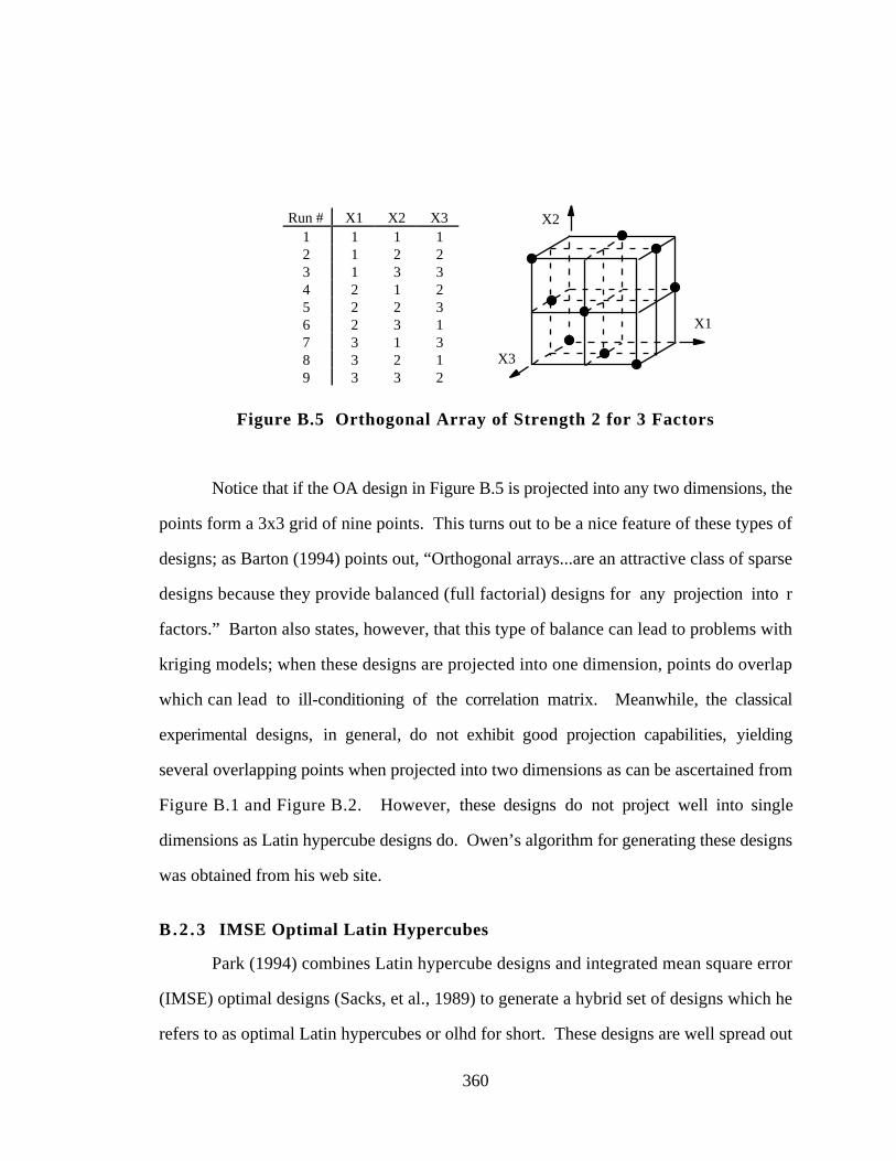
360
Run # X1 X2 X31 1 1 12 1 2 23 1 3 34 2 1 25 2 2 36 2 3 17 3 1 38 3 2 19 3 3 2
X1
X2
X3
Figure B.5 Orthogonal Array of Strength 2 for 3 Factors
Notice that if the OA design in Figure B.5 is projected into any two dimensions, the
points form a 3x3 grid of nine points. This turns out to be a nice feature of these types of
designs; as Barton (1994) points out, “Orthogonal arrays...are an attractive class of sparse
designs because they provide balanced (full factorial) designs for any projection into r
factors.” Barton also states, however, that this type of balance can lead to problems with
kriging models; when these designs are projected into one dimension, points do overlap
which can lead to ill-conditioning of the correlation matrix. Meanwhile, the classical
experimental designs, in general, do not exhibit good projection capabilities, yielding
several overlapping points when projected into two dimensions as can be ascertained from
Figure B.1 and Figure B.2. However, these designs do not project well into single
dimensions as Latin hypercube designs do. Owen’s algorithm for generating these designs
was obtained from his web site.
B.2 .3 IMSE Optimal Latin Hypercubes
Park (1994) combines Latin hypercube designs and integrated mean square error
(IMSE) optimal designs (Sacks, et al., 1989) to generate a hybrid set of designs which he
refers to as optimal Latin hypercubes or olhd for short. These designs are well spread out
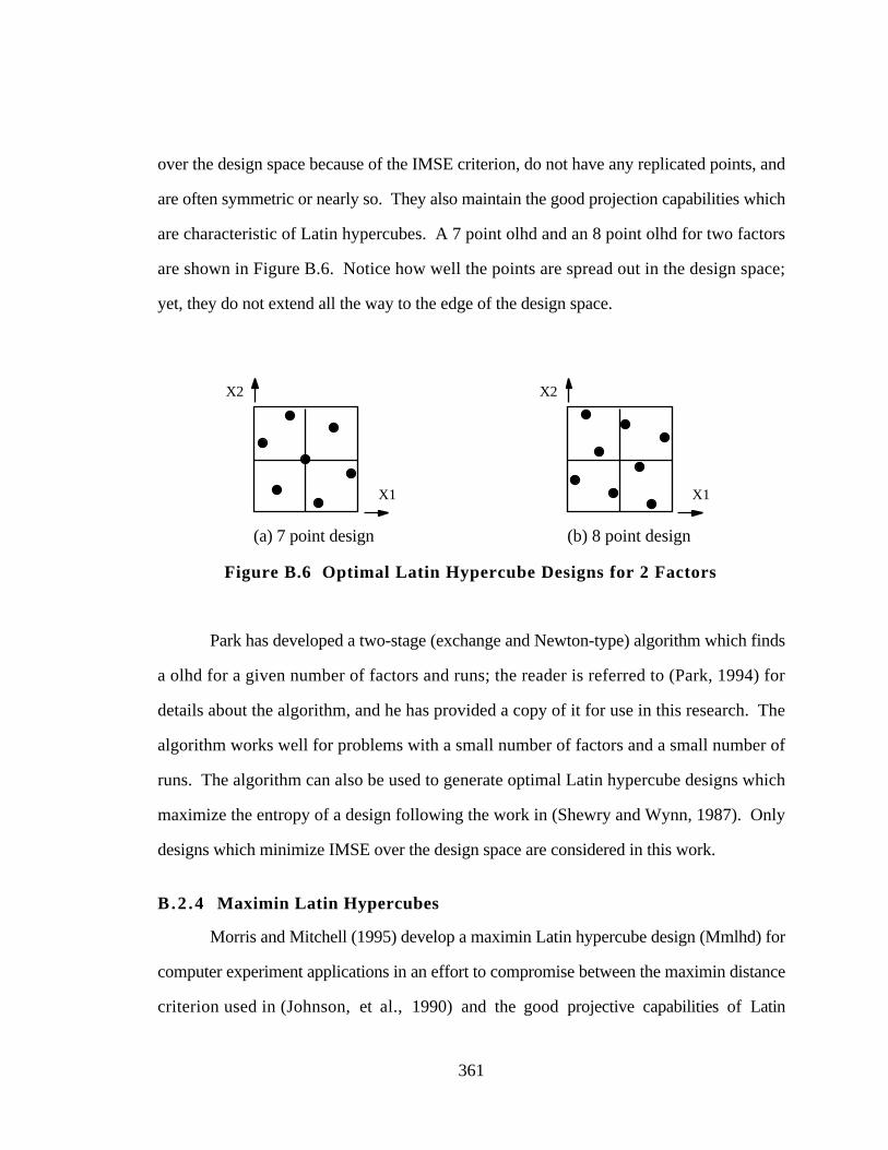
361
over the design space because of the IMSE criterion, do not have any replicated points, and
are often symmetric or nearly so. They also maintain the good projection capabilities which
are characteristic of Latin hypercubes. A 7 point olhd and an 8 point olhd for two factors
are shown in Figure B.6. Notice how well the points are spread out in the design space;
yet, they do not extend all the way to the edge of the design space.
X1
X2
X1
X2
(a) 7 point design (b) 8 point design
Figure B.6 Optimal Latin Hypercube Designs for 2 Factors
Park has developed a two-stage (exchange and Newton-type) algorithm which finds
a olhd for a given number of factors and runs; the reader is referred to (Park, 1994) for
details about the algorithm, and he has provided a copy of it for use in this research. The
algorithm works well for problems with a small number of factors and a small number of
runs. The algorithm can also be used to generate optimal Latin hypercube designs which
maximize the entropy of a design following the work in (Shewry and Wynn, 1987). Only
designs which minimize IMSE over the design space are considered in this work.
B.2 .4 Maximin Latin Hypercubes
Morris and Mitchell (1995) develop a maximin Latin hypercube design (Mmlhd) for
computer experiment applications in an effort to compromise between the maximin distance
criterion used in (Johnson, et al., 1990) and the good projective capabilities of Latin
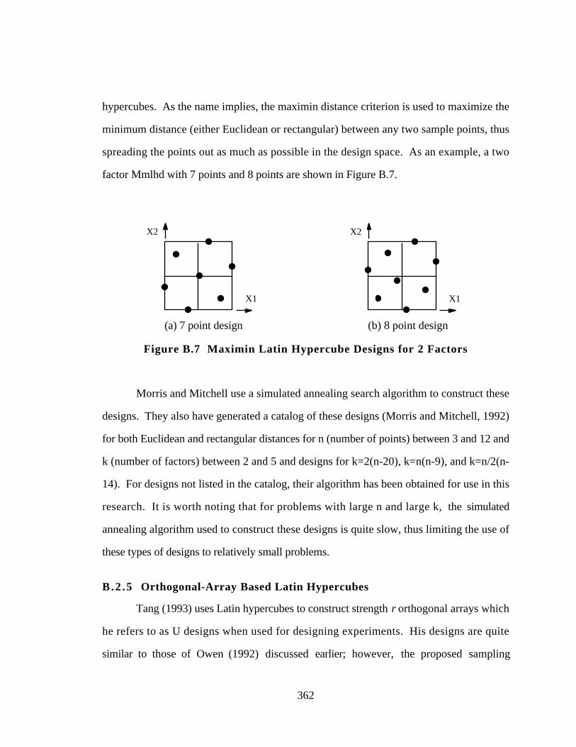
362
hypercubes. As the name implies, the maximin distance criterion is used to maximize the
minimum distance (either Euclidean or rectangular) between any two sample points, thus
spreading the points out as much as possible in the design space. As an example, a two
factor Mmlhd with 7 points and 8 points are shown in Figure B.7.
X1
X2
X1
X2
(a) 7 point design (b) 8 point design
Figure B.7 Maximin Latin Hypercube Designs for 2 Factors
Morris and Mitchell use a simulated annealing search algorithm to construct these
designs. They also have generated a catalog of these designs (Morris and Mitchell, 1992)
for both Euclidean and rectangular distances for n (number of points) between 3 and 12 and
k (number of factors) between 2 and 5 and designs for k=2(n-20), k=n(n-9), and k=n/2(n-
14). For designs not listed in the catalog, their algorithm has been obtained for use in this
research. It is worth noting that for problems with large n and large k, the simulated
annealing algorithm used to construct these designs is quite slow, thus limiting the use of
these types of designs to relatively small problems.
B.2 .5 Orthogonal-Array Based Latin Hypercubes
Tang (1993) uses Latin hypercubes to construct strength r orthogonal arrays which
he refers to as U designs when used for designing experiments. His designs are quite
similar to those of Owen (1992) discussed earlier; however, the proposed sampling
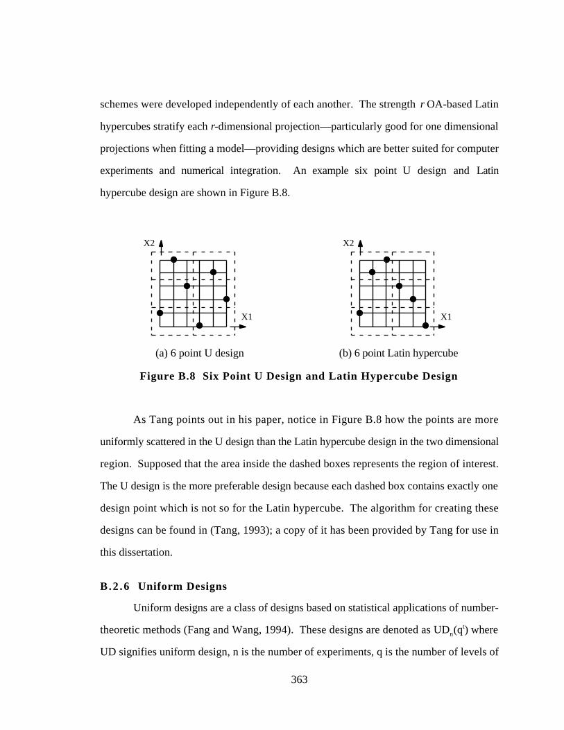
363
schemes were developed independently of each another. The strength r OA-based Latin
hypercubes stratify each r-dimensional projection—particularly good for one dimensional
projections when fitting a model—providing designs which are better suited for computer
experiments and numerical integration. An example six point U design and Latin
hypercube design are shown in Figure B.8.
X1
X2
X1
X2
(a) 6 point U design (b) 6 point Latin hypercube
Figure B.8 Six Point U Design and Latin Hypercube Design
As Tang points out in his paper, notice in Figure B.8 how the points are more
uniformly scattered in the U design than the Latin hypercube design in the two dimensional
region. Supposed that the area inside the dashed boxes represents the region of interest.
The U design is the more preferable design because each dashed box contains exactly one
design point which is not so for the Latin hypercube. The algorithm for creating these
designs can be found in (Tang, 1993); a copy of it has been provided by Tang for use in
this dissertation.
B.2 .6 Uniform Designs
Uniform designs are a class of designs based on statistical applications of number-
theoretic methods (Fang and Wang, 1994). These designs are denoted as UDn(qt) where
UD signifies uniform design, n is the number of experiments, q is the number of levels of
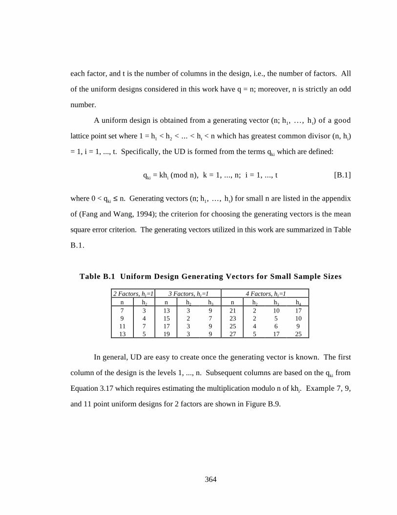
364
each factor, and t is the number of columns in the design, i.e., the number of factors. All
of the uniform designs considered in this work have q = n; moreover, n is strictly an odd
number.
A uniform design is obtained from a generating vector (n; h1, . . . , h t) of a good
lattice point set where 1 = h1 < h2 < ... < ht < n which has greatest common divisor (n, hi)
= 1, i = 1, ..., t. Specifically, the UD is formed from the terms qki which are defined:
qki = khi (mod n), k = 1, ..., n; i = 1, ..., t [B.1]
where 0 < qki ≤ n. Generating vectors (n; h1, ..., h t) for small n are listed in the appendix
of (Fang and Wang, 1994); the criterion for choosing the generating vectors is the mean
square error criterion. The generating vectors utilized in this work are summarized in Table
B.1.
Table B.1 Uniform Design Generating Vectors for Small Sample Sizes
2 Factors, h1=1 3 Factors, h1=1 4 Factors, h1=1n h2 n h2 h3 n h2 h3 h4
7 3 13 3 9 21 2 10 179 4 15 2 7 23 2 5 1011 7 17 3 9 25 4 6 913 5 19 3 9 27 5 17 25
In general, UD are easy to create once the generating vector is known. The first
column of the design is the levels 1, ..., n. Subsequent columns are based on the qki from
Equation 3.17 which requires estimating the multiplication modulo n of khi. Example 7, 9,
and 11 point uniform designs for 2 factors are shown in Figure B.9.
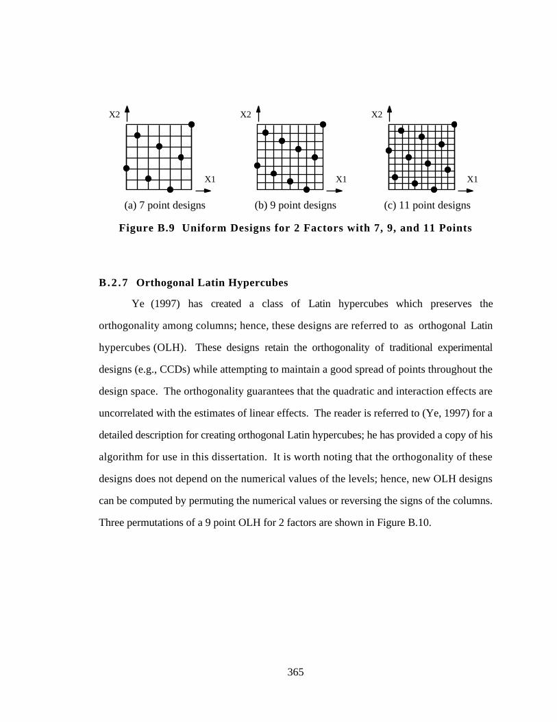
365
X1
X2
X1
X2
X1
X2
(a) 7 point designs (b) 9 point designs (c) 11 point designs
Figure B.9 Uniform Designs for 2 Factors with 7, 9, and 11 Points
B.2 .7 Orthogonal Latin Hypercubes
Ye (1997) has created a class of Latin hypercubes which preserves the
orthogonality among columns; hence, these designs are referred to as orthogonal Latin
hypercubes (OLH). These designs retain the orthogonality of traditional experimental
designs (e.g., CCDs) while attempting to maintain a good spread of points throughout the
design space. The orthogonality guarantees that the quadratic and interaction effects are
uncorrelated with the estimates of linear effects. The reader is referred to (Ye, 1997) for a
detailed description for creating orthogonal Latin hypercubes; he has provided a copy of his
algorithm for use in this dissertation. It is worth noting that the orthogonality of these
designs does not depend on the numerical values of the levels; hence, new OLH designs
can be computed by permuting the numerical values or reversing the signs of the columns.
Three permutations of a 9 point OLH for 2 factors are shown in Figure B.10.
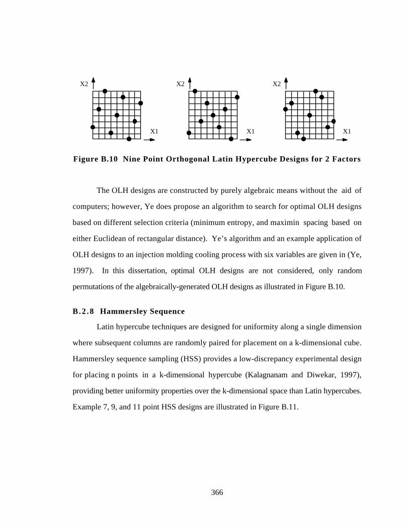
366
X1
X2
X1
X2
X1
X2
Figure B.10 Nine Point Orthogonal Latin Hypercube Designs for 2 Factors
The OLH designs are constructed by purely algebraic means without the aid of
computers; however, Ye does propose an algorithm to search for optimal OLH designs
based on different selection criteria (minimum entropy, and maximin spacing based on
either Euclidean of rectangular distance). Ye’s algorithm and an example application of
OLH designs to an injection molding cooling process with six variables are given in (Ye,
1997). In this dissertation, optimal OLH designs are not considered, only random
permutations of the algebraically-generated OLH designs as illustrated in Figure B.10.
B.2 .8 Hammersley Sequence
Latin hypercube techniques are designed for uniformity along a single dimension
where subsequent columns are randomly paired for placement on a k-dimensional cube.
Hammersley sequence sampling (HSS) provides a low-discrepancy experimental design
for placing n points in a k-dimensional hypercube (Kalagnanam and Diwekar, 1997),
providing better uniformity properties over the k-dimensional space than Latin hypercubes.
Example 7, 9, and 11 point HSS designs are illustrated in Figure B.11.
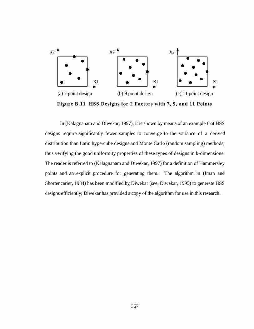
367
X1
X2
X1
X2
X1
X2
(a) 7 point design (b) 9 point design (c) 11 point design
Figure B.11 HSS Designs for 2 Factors with 7, 9, and 11 Points
In (Kalagnanam and Diwekar, 1997), it is shown by means of an example that HSS
designs require significantly fewer samples to converge to the variance of a derived
distribution than Latin hypercube designs and Monte Carlo (random sampling) methods,
thus verifying the good uniformity properties of these types of designs in k-dimensions.
The reader is referred to (Kalagnanam and Diwekar, 1997) for a definition of Hammersley
points and an explicit procedure for generating them. The algorithm in (Iman and
Shortencarier, 1984) has been modified by Diwekar (see, Diwekar, 1995) to generate HSS
designs efficiently; Diwekar has provided a copy of the algorithm for use in this research.
368
C. APPENDIX C
A MINIMAX LATIN HYPERCUBE DESIGNGENERATOR USING A GENETIC ALGORITHM
The details of the minimax Latin hypercube design which are unique to this
dissertation are presented in this appendix. In Section C.1 the question of “Why a minimax
Latin hypercube design?” is addressed. The genetic algorithm which is used to generate
these designs is then presented in Section C.2. Convergence studies of the genetic
algorithm are included in Section C.3.

369
C.1 WHY A MINIMAX LATIN HYPERCUBE DESIGN?
From an intuitive stand point, since prediction with a kriging model relies on the
spatial correlation between data points, a design which minimizes the maximum distance
between the sample points and any point in the design space should yield an accurate
predictor. This type of design is referred to as a minimax design (Johnson, et al., 1990).
Thus, the novel space filling design advocated in this work is the combination of the
minimax criterion with a Latin hypercube design. Why combine the two? Alone, the
minimax criterion does not ensure good stratification of the design space, i.e., when the
sample points are projected into 1-dimension, many of the points may overlap. Because a
Latin hypercube ensures good stratification of the design space when projected into 1-
dimension, the minimax criterion combined with a Latin hypercube design provides a good
compromise between minimizing the maximum distance between the sample points and any
point in the design space and the good projection properties of the Latin hypercube. Morris
and Mitchell (1995) used a similar argument when combining the maximin criterion with
Latin hypercubes to create maximin Latin hypercube designs; their designs performed better
than Latin hypercube designs and maximin designs in comparative studies.
How are these novel designs created? The algorithm provided by Morris and
Mitchell (1995) could not be modified easily to accommodate the minimax criterion as
opposed to the maximin criteria. Moreover, their use of a simulated annealing algorithm to
generate maximin Latin hypercube designs is slow at best. Thus, an entirely different
approach for generating minimax Latin hypercube designs was conceived.
Consider that a Latin hypercube is a (n x k) matrix which has n runs with n levels
for k factors. Since each column of the Latin hypercube contains a random permutation of
n numbers, there are n! possible permutations for each of k columns, yielding a total of
(n!)k possible combinations. For large n and k, an exhaustive search of all possible
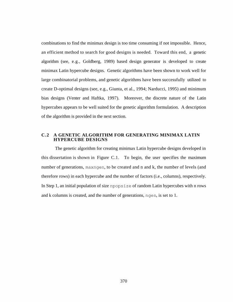
370
combinations to find the minimax design is too time consuming if not impossible. Hence,
an efficient method to search for good designs is needed. Toward this end, a genetic
algorithm (see, e.g., Goldberg, 1989) based design generator is developed to create
minimax Latin hypercube designs. Genetic algorithms have been shown to work well for
large combinatorial problems, and genetic algorithms have been successfully utilized to
create D-optimal designs (see, e.g., Giunta, et al., 1994; Narducci, 1995) and minimum
bias designs (Venter and Haftka, 1997). Moreover, the discrete nature of the Latin
hypercubes appears to be well suited for the genetic algorithm formulation. A description
of the algorithm is provided in the next section.
C.2 A GENETIC ALGORITHM FOR GENERATING MINIMAX LATINHYPERCUBE DESIGNS
The genetic algorithm for creating minimax Latin hypercube designs developed in
this dissertation is shown in Figure C.1. To begin, the user specifies the maximum
number of generations, maxngen, to be created and n and k, the number of levels (and
therefore rows) in each hypercube and the number of factors (i.e., columns), respectively.
In Step 1, an initial population of size npopsize of random Latin hypercubes with n rows
and k columns is created, and the number of generations, ngen, is set to 1.
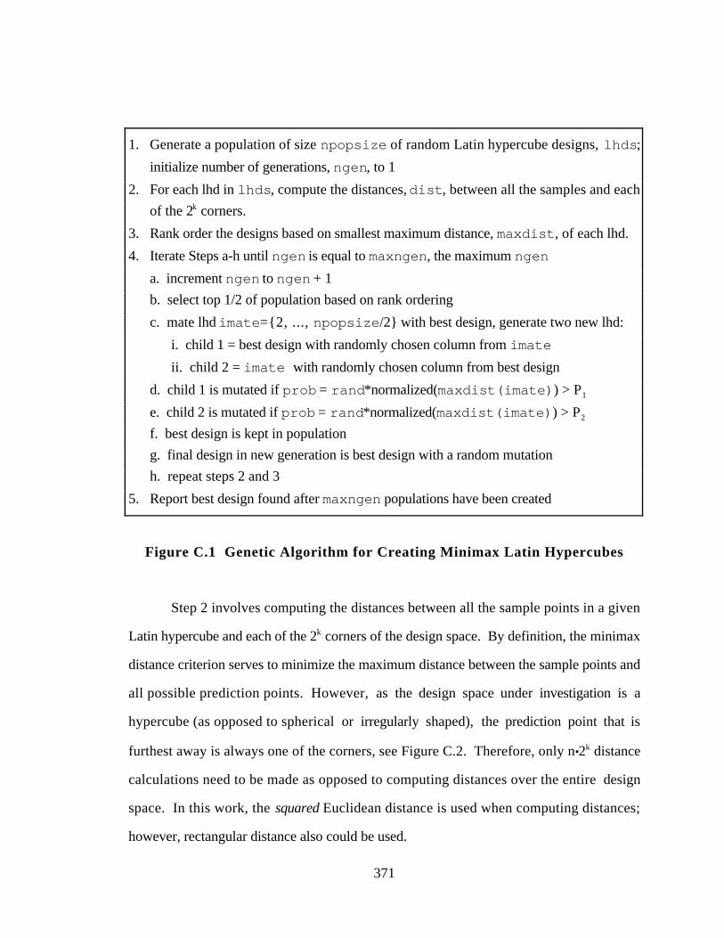
371
1. Generate a population of size npopsize of random Latin hypercube designs, lhds;
initialize number of generations, ngen, to 1
2. For each lhd in lhds, compute the distances, dist, between all the samples and each
of the 2k corners.
3. Rank order the designs based on smallest maximum distance, maxdist, of each lhd.
4. Iterate Steps a-h until ngen is equal to maxngen, the maximum ngen
a. increment ngen to ngen + 1
b. select top 1/2 of population based on rank ordering
c. mate lhd imate={2, ..., npopsize/2} with best design, generate two new lhd:
i. child 1 = best design with randomly chosen column from imate
ii. child 2 = imate with randomly chosen column from best design
d. child 1 is mutated if prob = rand*normalized(maxdist(imate)) > P1
e. child 2 is mutated if prob = rand*normalized(maxdist(imate)) > P2
f. best design is kept in population
g. final design in new generation is best design with a random mutation
h. repeat steps 2 and 3
5. Report best design found after maxngen populations have been created
Figure C.1 Genetic Algorithm for Creating Minimax Latin Hypercubes
Step 2 involves computing the distances between all the sample points in a given
Latin hypercube and each of the 2k corners of the design space. By definition, the minimax
distance criterion serves to minimize the maximum distance between the sample points and
all possible prediction points. However, as the design space under investigation is a
hypercube (as opposed to spherical or irregularly shaped), the prediction point that is
furthest away is always one of the corners, see Figure C.2. Therefore, only n•2k distance
calculations need to be made as opposed to computing distances over the entire design
space. In this work, the squared Euclidean distance is used when computing distances;
however, rectangular distance also could be used.
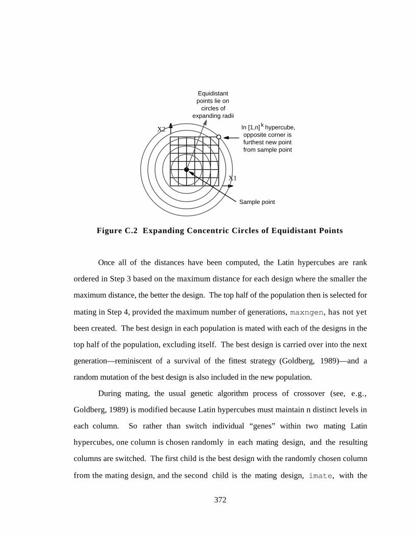
372
X1
X2
Equidistant points lie on
circles of expanding radii
Sample point
In [1,n] hypercube,opposite corner is furthest new point from sample point
k
Figure C.2 Expanding Concentric Circles of Equidistant Points
Once all of the distances have been computed, the Latin hypercubes are rank
ordered in Step 3 based on the maximum distance for each design where the smaller the
maximum distance, the better the design. The top half of the population then is selected for
mating in Step 4, provided the maximum number of generations, maxngen, has not yet
been created. The best design in each population is mated with each of the designs in the
top half of the population, excluding itself. The best design is carried over into the next
generation—reminiscent of a survival of the fittest strategy (Goldberg, 1989)—and a
random mutation of the best design is also included in the new population.
During mating, the usual genetic algorithm process of crossover (see, e.g.,
Goldberg, 1989) is modified because Latin hypercubes must maintain n distinct levels in
each column. So rather than switch individual “genes” within two mating Latin
hypercubes, one column is chosen randomly in each mating design, and the resulting
columns are switched. The first child is the best design with the randomly chosen column
from the mating design, and the second child is the mating design, imate, with the

373
randomly chosen column form the best design. After mating is done, mutation may occur.
Child 1 undergoes mutation if the probability P = (random number)(normalized maximum
distance of imate) is greater than P1; Child 2 undergoes mutation if the probability P =
(random number)(normalized maximum distance of imate) is greater than P2. When
computing the probability, normalization of the maximum distance is taken as:
normalized maxdist = maxdist − maxdistmin
maxdist max − maxdist min
[C.1]
where maxdistmax and maxdistmin are for the entire population before mating. In this
manner, the larger (worse) the maximum distance of the parent design, the greater the
probability that its child (Child 2) will undergo a mutation in hopes of further reducing its
maximum distance after mating. Meanwhile, since the normalized maximum distance of
the best design is zero, the probability of mutating Child 1 is also based on the normalized
distance of the mating parent, but the probability of mutation, P1, is higher than P2 because
this design has more in common with the best design and therefore need not mutate as
often.
Once a new population has been created, Steps 2 and 3 are repeated, computing the
distances between the sample points and the corners and rank ordering the designs based
on smaller maximum distance being better. The best 1/2 of the population is then mated
and mutated again as the minimax distance Latin hypercube is sought. A pictorial
illustration of the mating and mutation process is shown in Figure C.3.
In Figure C.3, an initial population of six Latin hypercube designs are generated
randomly. In this example, each Latin hypercube has five sample points for two factors as
illustrated in the 2-D grids of sample points. Once these designs are created, the distance
between each point and each corner is computed, and the maximum distance is recorded.
Multiple points can have the same maximum distance; hence, the number of points having
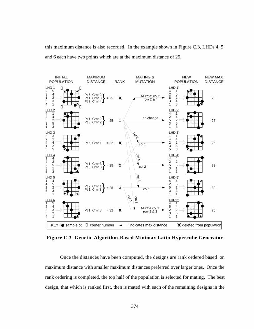
374
this maximum distance is also recorded. In the example shown in Figure C.3, LHDs 4, 5,
and 6 each have two points which are at the maximum distance of 25.
5
6x
x
INITIALPOPULATION
MAXIMUMDISTANCE RANK
NEWPOPULATION
LHD 24 12 45 23 51 3
LHD 41 44 22 53 15 3
LHD 61 52 43 35 24 1
LHD 33 32 14 41 25 5
LHD 12 53 41 25 34 1
➀
➁ ➃
➂
Pt 5, Crnr 2Pt 1, Crnr 3Pt 3, Crnr 4
= 25}
Pt 1, Crnr 3 = 32
Pt 1, Crnr 2Pt 3, Crnr 2 = 25}
= 25}Pt 1, Crnr 3Pt 3, Crnr 3
4
1
LHD 51 44 52 25 33 1
= 25}Pt 2, Crnr 1Pt 1, Crnr 3
MATING &MUTATION
LHD 2’4 12 45 23 51 3
LHD 6’4 15 42 23 51 3
LHD 4’4 42 25 53 11 3
LHD 3’1 14 42 23 55 3
LHD 1’4 12 55 23 41 3
25
25
32
32
25
NEW MAXDISTANCE
x
Mutate col 1 row 2 & 3
col 2
Mutate: col 2row 2 & 4
col 1
col 2
col 1
col 2
col 2no change
25= 32Pt 5, Crnr 1 col 1
col 1
2
3
LHD 5’4 42 55 23 31 1
indicates max distancesample pt ➀ corner numberKEY: x deleted from population
Figure C.3 Genetic Algorithm-Based Minimax Latin Hypercube Generator
Once the distances have been computed, the designs are rank ordered based on
maximum distance with smaller maximum distances preferred over larger ones. Once the
rank ordering is completed, the top half of the population is selected for mating. The best
design, that which is ranked first, then is mated with each of the remaining designs in the
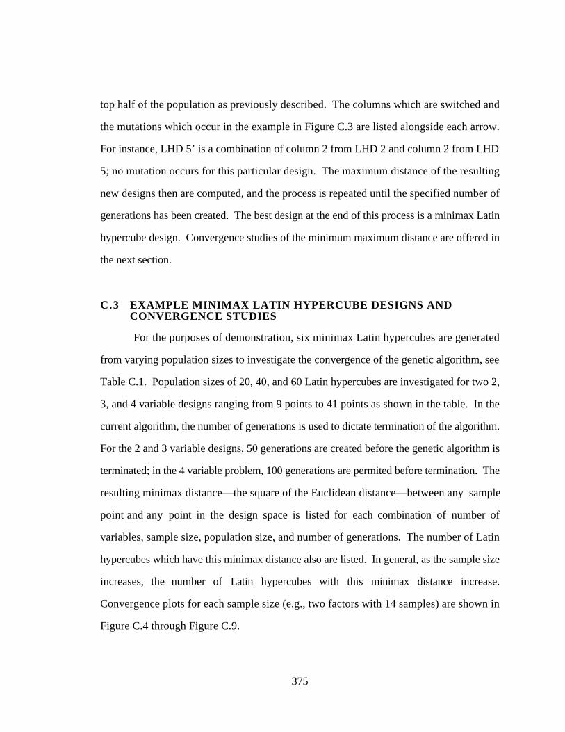
375
top half of the population as previously described. The columns which are switched and
the mutations which occur in the example in Figure C.3 are listed alongside each arrow.
For instance, LHD 5’ is a combination of column 2 from LHD 2 and column 2 from LHD
5; no mutation occurs for this particular design. The maximum distance of the resulting
new designs then are computed, and the process is repeated until the specified number of
generations has been created. The best design at the end of this process is a minimax Latin
hypercube design. Convergence studies of the minimum maximum distance are offered in
the next section.
C.3 EXAMPLE MINIMAX LATIN HYPERCUBE DESIGNS ANDCONVERGENCE STUDIES
For the purposes of demonstration, six minimax Latin hypercubes are generated
from varying population sizes to investigate the convergence of the genetic algorithm, see
Table C.1. Population sizes of 20, 40, and 60 Latin hypercubes are investigated for two 2,
3, and 4 variable designs ranging from 9 points to 41 points as shown in the table. In the
current algorithm, the number of generations is used to dictate termination of the algorithm.
For the 2 and 3 variable designs, 50 generations are created before the genetic algorithm is
terminated; in the 4 variable problem, 100 generations are permited before termination. The
resulting minimax distance—the square of the Euclidean distance—between any sample
point and any point in the design space is listed for each combination of number of
variables, sample size, population size, and number of generations. The number of Latin
hypercubes which have this minimax distance also are listed. In general, as the sample size
increases, the number of Latin hypercubes with this minimax distance increase.
Convergence plots for each sample size (e.g., two factors with 14 samples) are shown in
Figure C.4 through Figure C.9.
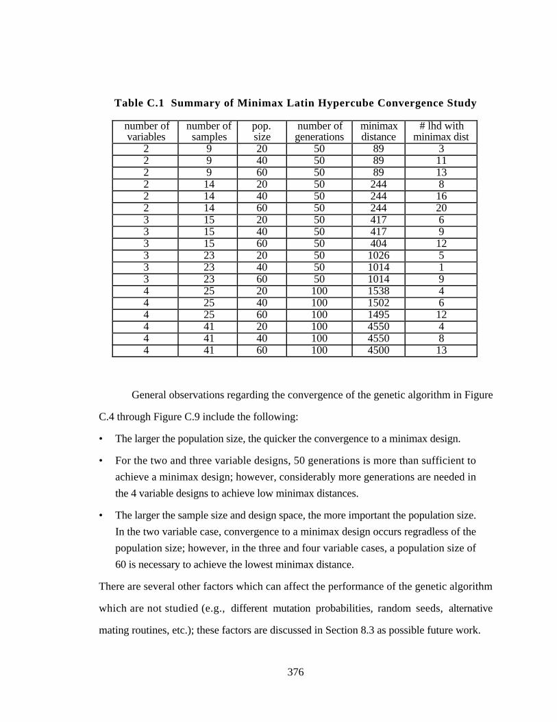
376
Table C.1 Summary of Minimax Latin Hypercube Convergence Study
number ofvariables
number ofsamples
pop.size
number ofgenerations
minimaxdistance
# lhd withminimax dist
2 9 20 50 89 32 9 40 50 89 112 9 60 50 89 132 14 20 50 244 82 14 40 50 244 162 14 60 50 244 203 15 20 50 417 63 15 40 50 417 93 15 60 50 404 123 23 20 50 1026 53 23 40 50 1014 13 23 60 50 1014 94 25 20 100 1538 44 25 40 100 1502 64 25 60 100 1495 124 41 20 100 4550 44 41 40 100 4550 84 41 60 100 4500 13
General observations regarding the convergence of the genetic algorithm in Figure
C.4 through Figure C.9 include the following:
• The larger the population size, the quicker the convergence to a minimax design.
• For the two and three variable designs, 50 generations is more than sufficient to
achieve a minimax design; however, considerably more generations are needed in
the 4 variable designs to achieve low minimax distances.
• The larger the sample size and design space, the more important the population size.
In the two variable case, convergence to a minimax design occurs regradless of the
population size; however, in the three and four variable cases, a population size of
60 is necessary to achieve the lowest minimax distance.
There are several other factors which can affect the performance of the genetic algorithm
which are not studied (e.g., different mutation probabilities, random seeds, alternative
mating routines, etc.); these factors are discussed in Section 8.3 as possible future work.
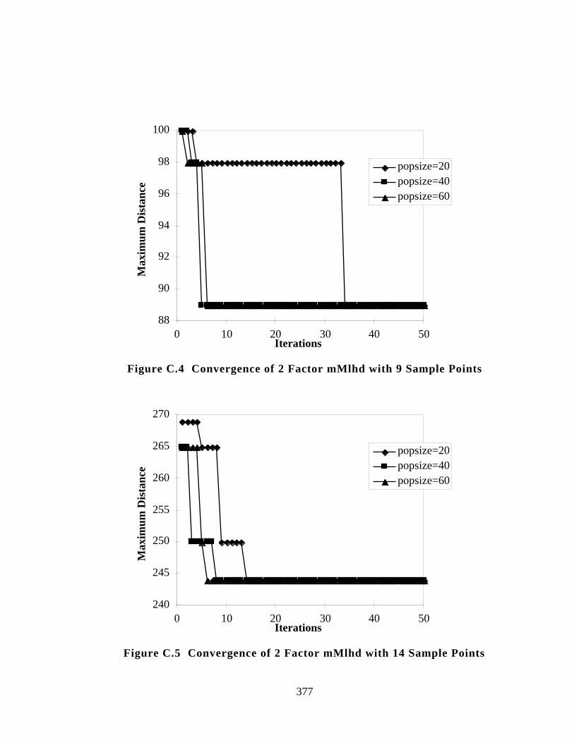
377
88
90
92
94
96
98
100
0 10 20 30 40 50Iterations
Max
imum
Dis
tanc
e
popsize=20popsize=40popsize=60
Figure C.4 Convergence of 2 Factor mMlhd with 9 Sample Points
240
245
250
255
260
265
270
0 10 20 30 40 50Iterations
Max
imum
Dis
tanc
e
popsize=20popsize=40popsize=60
Figure C.5 Convergence of 2 Factor mMlhd with 14 Sample Points
378
400
405
410
415
420
425
430
435
440
445
0 10 20 30 40 50Iterations
Max
imum
Dis
tanc
epopsize=20popsize=40popsize=60
Figure C.6 Convergence of 3 Factor mMlhd with 15 Sample Points
1010
1020
1030
1040
1050
1060
1070
0 10 20 30 40 50Iterations
Max
imum
Dis
tanc
e
popsize=20popsize=40popsize=60
Figure C.7 Convergence of 3 Factor mMlhd with 23 Sample Points
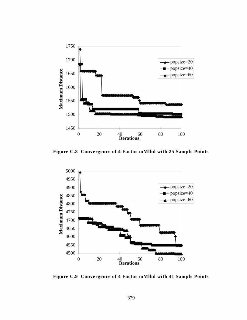
379
1450
1500
1550
1600
1650
1700
1750
0 20 40 60 80 100Iterations
Max
imum
Dis
tanc
epopsize=20popsize=40popsize=60
Figure C.8 Convergence of 4 Factor mMlhd with 25 Sample Points
4500
4550
4600
4650
4700
4750
4800
4850
4900
4950
5000
0 20 40 60 80 100Iterations
Max
imum
Dis
tanc
e
popsize=20popsize=40popsize=60
Figure C.9 Convergence of 4 Factor mMlhd with 41 Sample Points

380
D. APPENDIX D
KRIGING TESTBED PROBLEMS
Kriging/DOE Testbed
In Chapter 5 six engineering test problems—consisting of 2 two variable problems,
2 three variable problems, and 2 four variable problems—are introduced to test the utility of
kriging and space filling experimental designs for building metamodels of deterministic
computer experiments. The two variable problems are the design of a two-bar truss,
Section D.1, and the design of a symmetric three bar truss, Section D.2; the three variable
problems are the design of a helical compression spring, Section D.3, and a two-member
frame, Section D.4; and the four variables problems are the design of a welded beam,
Section D.5, and a pressure vessel, Section D.6. As explained in Section 5.1.1, building
kriging approximations of these analyses is overkill to say the least; however, they are
taken to be representative of typical analyses encountered in mechanical engineering design,
allowing Hypotheses 2 and 3 to be tested and verified. Each example is described in turn
along with its corresponding constraints, bounds, and objective function.

381
D.1 DESIGN OF A TWO-BAR TRUSS
The symmetric two-bar truss shown in Figure D.1 has been studied by several
researchers (see, e.g., Balling and Clark, 1992; Schmit, 1981; Sobieszczanski-Sobieski, et
al., 1982). In this example, a single load case of 2P = 66,000 lbs is considered. The
distance between the supports is 2B = 60 in. The two bars are identical, having an annular
cross section with wall thickness T = 0.1 in. The material properties are Young’s modulus
E = 30E6 psi, density ρ = 0.3 lbs/in3 and yield stress σy = 60,000 psi. There are two
design variables—mean tube diameter (D) and height (H) of the truss—which have the
following ranges of interest:
0.5 in. ≤ D ≤ 5 in.5 in. ≤ H ≤ 50 in.
t
D
Section C-C’
H2P
B B
C
C’
Figure D.1 Two-Bar Truss
The objective is to minimize the weight of truss system which is:
W(x) = 2ρπDT(B2 + H2)1/2 [D.1]
382
subject to the following behavioral constraints:
g1(x) = σe - σ = π 2E(D2 + T2)
8(B2 + H2 )−
P(B2 + H2)1/2
πTDH ≥ 0 [D.2]
g2(x) = σy - σ = σy - P(B2 + H2)1/2
πTDH ≥ 0 [D.3]
The first constraint prevents failure due to Euler buckling, the second due to yield. The
resulting optimum value from (Schmit, 1981) for W(x) is 19.8 lbs, occurring at:
D* = 2.47 in.H* = 30.15 in.
Hence, two constraints—Equations D.1 and D.2—and one objective function—
Equation D.3—are to be replaced by kriging models. These three equations are to be
approximated over the region of interest specified by the bounds on the two design
variables given at the beginning of this section. The next example is another two variable,
structural optimization problem.
D.2 DESIGN OF A SYMMETRIC THREE-BAR TRUSS
The second example also comes from (Schmit, 1981); it is the design of a
symmetric three-bar planar truss, see Figure D.2. Two loads are considered: P1 = 20,000
lbs acting at 45° to the x axis and P2 = 20,000 lbs acting at an angle of 135° to the axis.
Pertinent design parameters include the following: N = 10 in., β1 = 135°, β1 = 90°, β1 = 45°,
density ρ = 0.1 lbs/in3 and Young’s modulus E = 10E6 psi.
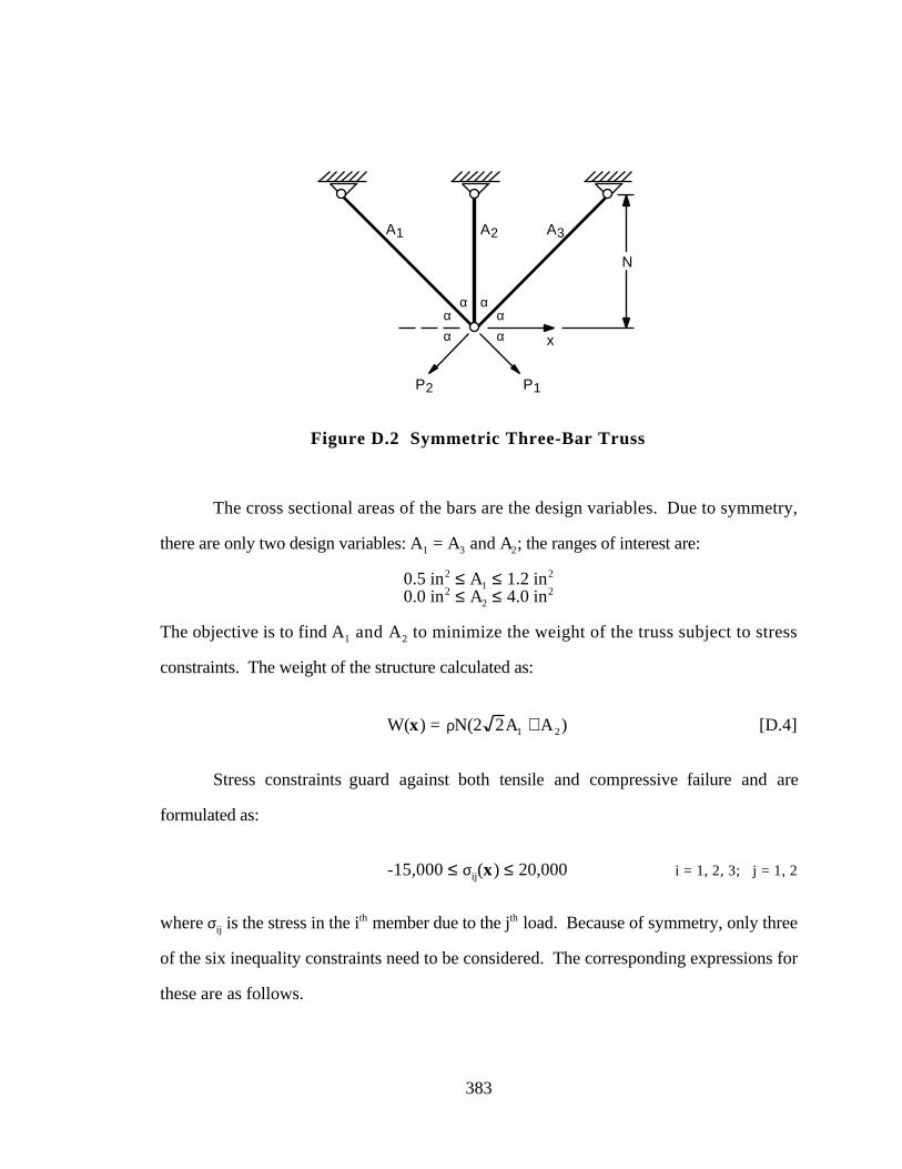
383
N
x
P1P2
αααα
αα
A1 A2 A3
Figure D.2 Symmetric Three-Bar Truss
The cross sectional areas of the bars are the design variables. Due to symmetry,
there are only two design variables: A1 = A3 and A2; the ranges of interest are:
0.5 in2 ≤ A1 ≤ 1.2 in2
0.0 in2 ≤ A2 ≤ 4.0 in2
The objective is to find A1 and A2 to minimize the weight of the truss subject to stress
constraints. The weight of the structure calculated as:
W(x) = ρN(2 2A1 + A2) [D.4]
Stress constraints guard against both tensile and compressive failure and are
formulated as:
-15,000 ≤ σij(x) ≤ 20,000 i = 1, 2, 3; j = 1, 2
where σij is the stress in the ith member due to the jth load. Because of symmetry, only three
of the six inequality constraints need to be considered. The corresponding expressions for
these are as follows.
384
g1(x) = 20,000 - σ11 = 20,000 - 1
A1
−A2
2A1A2 + 2A12
≥ 0 [D.5]
g1(x) = 20,000 - σ21 = 20,000 - 20,000 2A1
2A1A2 + 2A12 ≥ 0 [D.6]
g1(x) = 15,000 + σ31 = 15,000 - −20,000A 2
2A 1A2 + 2A12 ≥ 0 [D.7]
The optimum value W(x) given in (Schmit, 1981) is 2.64 lbs, occurring at:
A1* = A1* = 0.788 in2
A2* = 0.41 in2
In summary, there are three constraints—Equations D.5-D.7—and one objective—
Equation D.4— which are to be replaced by kriging models for the design space defined by
the bounds on A1 and A2. This concludes the two variables examples considered in this
dissertation; the first three variable problem, the design of a helical compression spring, is
detailed in the next section.
D.3 DESIGN OF A HELICAL COMPRESSION SPRING
A problem which is perhaps more representative of traditional mechanical
engineering design is the design of a helical compression spring (Kannan and Kramer,
1994; Sandgren, 1990; Siddall, 1982), see Figure D.2. There are three design variables—
number of active coils (N), mean coil diameter (D), and wire diameter (d)—with the
following ranges of interest:
3 ≤ N ≤ 301.0 in. ≤ D ≤ 6.0 in.0.2 in. ≤ d ≤ 0.5 in.
The spring is to be manufactured from music wire spring steel ASTM A228; the
maximum outside diameter, Dmax, must be less than 3 in. The allowable stress is S =
189,000 psi, and the shear modulus is G = 1.15E8. The maximum working load is Fmax =
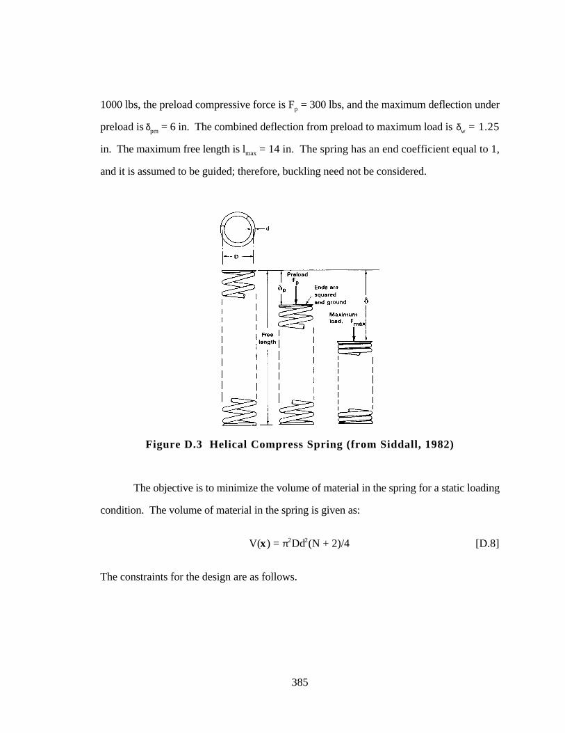
385
1000 lbs, the preload compressive force is Fp = 300 lbs, and the maximum deflection under
preload is δpm = 6 in. The combined deflection from preload to maximum load is δw = 1.25
in. The maximum free length is lmax = 14 in. The spring has an end coefficient equal to 1,
and it is assumed to be guided; therefore, buckling need not be considered.
Figure D.3 Helical Compress Spring (from Siddall, 1982)
The objective is to minimize the volume of material in the spring for a static loading
condition. The volume of material in the spring is given as:
V(x) = π2Dd2(N + 2)/4 [D.8]
The constraints for the design are as follows.
386
D.3.1 Shear Stress
Following the problem formulations given in (Kannan and Kramer, 1994;
Sandgren, 1990; Siddall, 1982), the design shear stress must be less than the allowable
maximum shear stress or:
g1(x) = S - 8CfFmaxD/(πd3) ≥ 0 [D.9]
where:
Cf = (4C - 1)/(4C - 4) + 0.615/C
C = D/d
In reality, the spring correction factor, Cf, given by the preceding equation is for
springs subject to dynamic loading and is only important when fatigue is a concern. In this
example, the spring is assumed to be under a constant load, and the correction factor which
should be used for a spring in static loading is (Shigley and Mischke, 1989):
Cf = 1 + 0.5/C
However, in order to maintain consistency with previous problem formulations and
solutions which are also in error, (see, Kannan and Kramer, 1994; Sandgren, 1990;
Siddall, 1982), the fatigue correction factor is used in this example since it is only for
demonstrative purposes.
D.3.2 Free Length
The spring free length must be less than the specified value:
g2(x) = lmax - lf ≥ 0 [D.10]
where:
387
lf = δ + 1.05(N + 2)d
δ = Fmax/K
K = Gd4/(8ND3)
This assumes that the spring length is 1.05 times the solid length under Fmax.
D.3.3 Preload Deflection
The deflection under preload must not exceed specified deflection δpm:
g3(x) = δpm - δ ≥ 0 [D.11]
D.3.4 Combined Deflections
The combined deflections must be consistent with the length
lf - δp - (Fmax - Fload)/K - 1.05(N + 2)d ≥ 0
where:
δp = Fp/K
As Siddall (1982) points out, this constraint function will always be zero at convergence;
therefore, it is not included in the problem formulation.
D.3.5 Deflection Requirement
The deflection from preload to maximum load must be equal to that specified:
g4(x) = (Fmax - Fload)/K - δw ≥ 0 [D.11]

388
D.3.6 Geometric Constraints
There are two additional geometric constraints which also must be satisfied. The
outside diameter of the coil must be less than the maximum specified:
g5(x) = Dmax - D - d ≥ 0 [D.12]
The inner coil diameter must be at least three times the wire diameter for proper winding:
g6(x) = C - 3 ≥ 0 [D.13]
This spring problem is typically solved using a mixed discrete/continuous solver.
The continuous solution which is given in (Sandgren, 1990) is V(x) = 2.6353 which
occurs at:
N* = 9.192D* = 1.2052 in.d* = 0.2814 in.
Hence, seven constraints—Equations D.9-D.13—and one objective function—
Equation D.8—are to be approximated using kriging models. The design region of interest
is defined by the bounds on the design variables given at the beginning of this section. The
design of a two-member frame presented in the next section is the other three variable test
problem being considered in this dissertation.
D.4 DESIGN OF A TWO-MEMBER FRAME
This example is from (Arora, 1989) and is the design of a two-member frame
subjected to the out-of-plane loads shown as in Figure D.4. There are three design
variables—frame width (d), height (h), and wall thickness (t)—with the following ranges
of interest:
2.5 in. ≤ d ≤ 10 in.2.5 in. ≤ h ≤ 10 in.
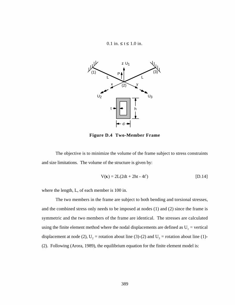
389
0.1 in. ≤ t ≤ 1.0 in.
ht
d
(1)
(2)
(3)LL
z
P
x y
U1
U2 U3
Figure D.4 Two-Member Frame
The objective is to minimize the volume of the frame subject to stress constraints
and size limitations. The volume of the structure is given by:
V(x) = 2L(2dt + 2ht - 4t2) [D.14]
where the length, L, of each member is 100 in.
The two members in the frame are subject to both bending and torsional stresses,
and the combined stress only needs to be imposed at nodes (1) and (2) since the frame is
symmetric and the two members of the frame are identical. The stresses are calculated
using the finite element method where the nodal displacements are defined as U1 = vertical
displacement at node (2), U2 = rotation about line (3)-(2) and U3 = rotation about line (1)-
(2). Following (Arora, 1989), the equilibrium equation for the finite element model is:
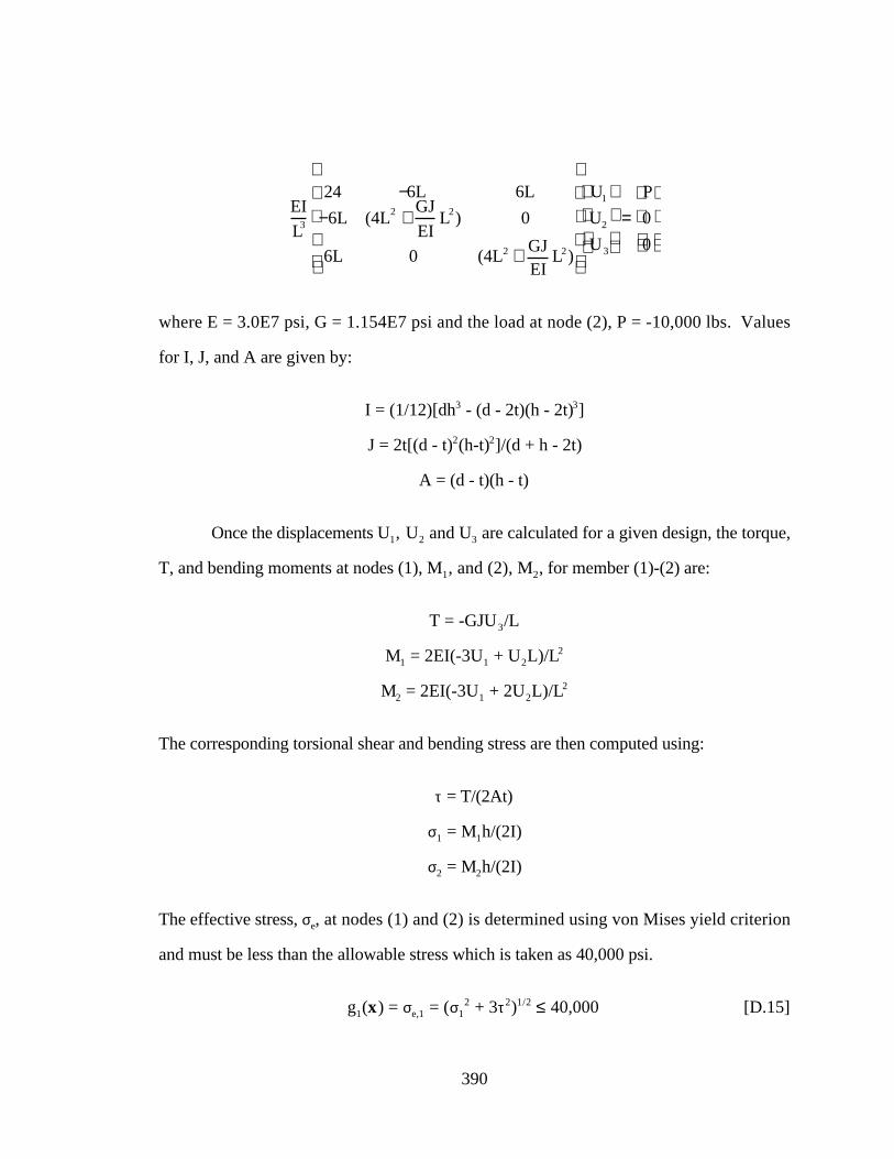
390
EI
L3
24 −6L 6L
−6L (4L2 +GJ
EIL2) 0
6L 0 (4L2 + GJEI
L2)
U1
U2
U3
=P
0
0
where E = 3.0E7 psi, G = 1.154E7 psi and the load at node (2), P = -10,000 lbs. Values
for I, J, and A are given by:
I = (1/12)[dh3 - (d - 2t)(h - 2t)3]
J = 2t[(d - t)2(h-t)2]/(d + h - 2t)
A = (d - t)(h - t)
Once the displacements U1, U2 and U3 are calculated for a given design, the torque,
T, and bending moments at nodes (1), M1, and (2), M2, for member (1)-(2) are:
T = -GJU3/L
M1 = 2EI(-3U1 + U2L)/L2
M2 = 2EI(-3U1 + 2U2L)/L2
The corresponding torsional shear and bending stress are then computed using:
τ = T/(2At)
σ1 = M1h/(2I)
σ2 = M2h/(2I)
The effective stress, σe, at nodes (1) and (2) is determined using von Mises yield criterion
and must be less than the allowable stress which is taken as 40,000 psi.
g1(x) = σe,1 = (σ12 + 3τ2)1/2 ≤ 40,000 [D.15]
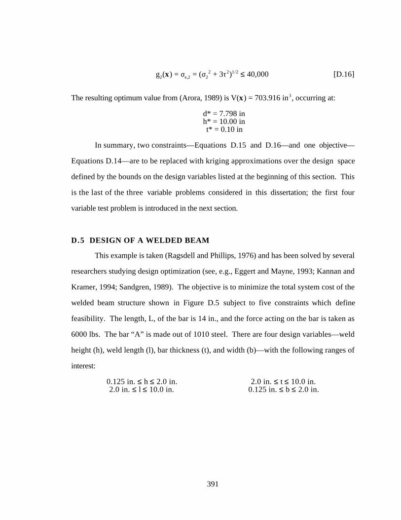
391
g2(x) = σe,2 = (σ22 + 3τ2)1/2 ≤ 40,000 [D.16]
The resulting optimum value from (Arora, 1989) is V(x) = 703.916 in3, occurring at:
d* = 7.798 inh* = 10.00 int* = 0.10 in
In summary, two constraints—Equations D.15 and D.16—and one objective—
Equations D.14—are to be replaced with kriging approximations over the design space
defined by the bounds on the design variables listed at the beginning of this section. This
is the last of the three variable problems considered in this dissertation; the first four
variable test problem is introduced in the next section.
D.5 DESIGN OF A WELDED BEAM
This example is taken (Ragsdell and Phillips, 1976) and has been solved by several
researchers studying design optimization (see, e.g., Eggert and Mayne, 1993; Kannan and
Kramer, 1994; Sandgren, 1989). The objective is to minimize the total system cost of the
welded beam structure shown in Figure D.5 subject to five constraints which define
feasibility. The length, L, of the bar is 14 in., and the force acting on the bar is taken as
6000 lbs. The bar “A” is made out of 1010 steel. There are four design variables—weld
height (h), weld length (l), bar thickness (t), and width (b)—with the following ranges of
interest:
0.125 in. ≤ h ≤ 2.0 in. 2.0 in. ≤ t ≤ 10.0 in.2.0 in. ≤ l ≤ 10.0 in. 0.125 in. ≤ b ≤ 2.0 in.

392
B
A
L
F
h
F
b
l t
Figure D.5 Welded Beam
The objective function is a combination of set-up cost, welding labor cost and
material cost and is given by:
F(x) = (1 + c3)h2l + c4tb(L + l) [D.17]
where c3 = (0.37)(0.283)($/in.) and c4 = (0.17)(0.283)($/in.). The constraints for the
problem include the maximum shear stress in the weld, the maximum normal stress in the
beam, the bar buckling load, the bar end deflection, and a geometric constraint which
ensures that the thickness of the weld, h, is less than the bar width, b, assuming a 45°
weldment. The necessary equations for the remaining constraints are as follows:
D.5.1 Weld Stress
The shear stress in the weld is given by:
τ(x) = [(τ’)2 + 2τ’τ’’cosθ + (τ’’)2]1/2 [D.18]
where:
cosθ = l/2R
R = {(l2/4) + [(t + h)/2]2}1/2
τ’ = F/ 2hl and τ’’ = MR/J
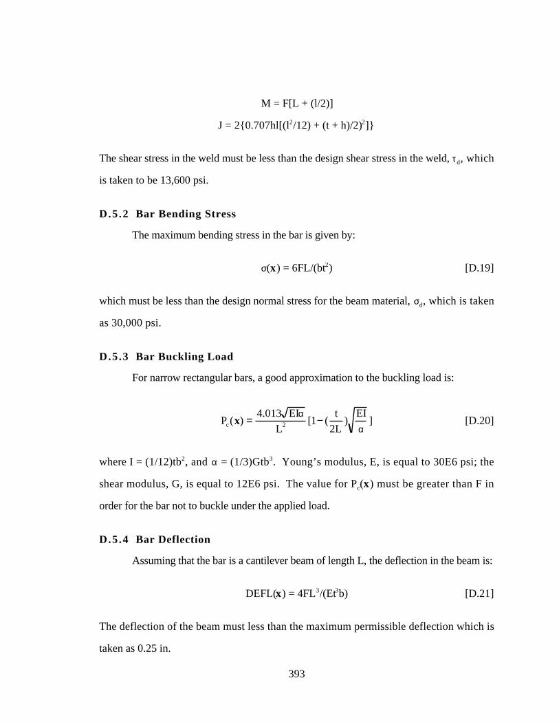
393
M = F[L + (l/2)]
J = 2{0.707hl[(l2/12) + (t + h)/2)2]}
The shear stress in the weld must be less than the design shear stress in the weld, τd, which
is taken to be 13,600 psi.
D.5.2 Bar Bending Stress
The maximum bending stress in the bar is given by:
σ(x) = 6FL/(bt2) [D.19]
which must be less than the design normal stress for the beam material, σd, which is taken
as 30,000 psi.
D.5.3 Bar Buckling Load
For narrow rectangular bars, a good approximation to the buckling load is:
Pc(x) =4.013 EIα
L2 [1− (t
2L)
EI
α] [D.20]
where I = (1/12)tb2, and α = (1/3)Gtb3. Young’s modulus, E, is equal to 30E6 psi; the
shear modulus, G, is equal to 12E6 psi. The value for Pc(x) must be greater than F in
order for the bar not to buckle under the applied load.
D.5.4 Bar Deflection
Assuming that the bar is a cantilever beam of length L, the deflection in the beam is:
DEFL(x) = 4FL3/(Et3b) [D.21]
The deflection of the beam must less than the maximum permissible deflection which is
taken as 0.25 in.
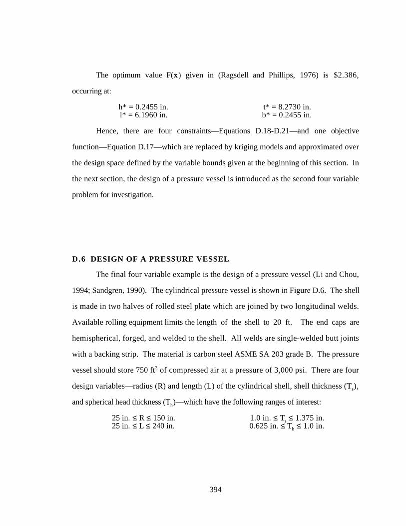
394
The optimum value F(x) given in (Ragsdell and Phillips, 1976) is $2.386,
occurring at:
h* = 0.2455 in. t* = 8.2730 in.l* = 6.1960 in. b* = 0.2455 in.
Hence, there are four constraints—Equations D.18-D.21—and one objective
function—Equation D.17—which are replaced by kriging models and approximated over
the design space defined by the variable bounds given at the beginning of this section. In
the next section, the design of a pressure vessel is introduced as the second four variable
problem for investigation.
D.6 DESIGN OF A PRESSURE VESSEL
The final four variable example is the design of a pressure vessel (Li and Chou,
1994; Sandgren, 1990). The cylindrical pressure vessel is shown in Figure D.6. The shell
is made in two halves of rolled steel plate which are joined by two longitudinal welds.
Available rolling equipment limits the length of the shell to 20 ft. The end caps are
hemispherical, forged, and welded to the shell. All welds are single-welded butt joints
with a backing strip. The material is carbon steel ASME SA 203 grade B. The pressure
vessel should store 750 ft3 of compressed air at a pressure of 3,000 psi. There are four
design variables—radius (R) and length (L) of the cylindrical shell, shell thickness (Ts),
and spherical head thickness (Th)—which have the following ranges of interest:
25 in. ≤ R ≤ 150 in. 1.0 in. ≤ Ts ≤ 1.375 in.25 in. ≤ L ≤ 240 in. 0.625 in. ≤ Th ≤ 1.0 in.
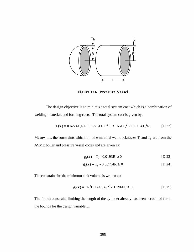
395
R
TsTh
R
L
Figure D.6 Pressure Vessel
The design objective is to minimize total system cost which is a combination of
welding, material, and forming costs. The total system cost is given by:
F(x) = 0.6224T sRL + 1.7781ThR2 + 3.1661T s
2L + 19.84Ts2R [D.22]
Meanwhile, the constraints which limit the minimal wall thicknesses Ts and Th are from the
ASME boiler and pressure vessel codes and are given as:
g1(x) = Ts - 0.0193R ≥ 0 [D.23]
g2(x) = Th - 0.00954R ≥ 0 [D.24]
The constraint for the minimum tank volume is written as:
g3(x) = πR2L + (4/3)πR3 - 1.296E6 ≥ 0 [D.25]
The fourth constraint limiting the length of the cylinder already has been accounted for in
the bounds for the design variable L.
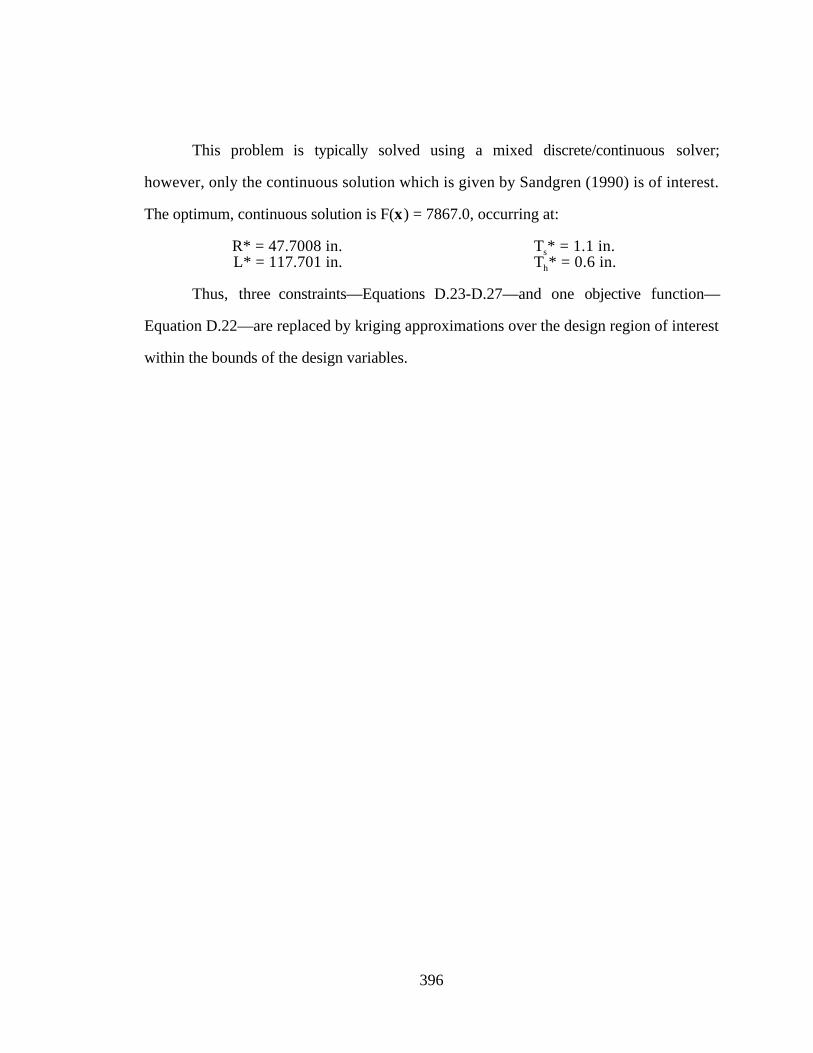
396
This problem is typically solved using a mixed discrete/continuous solver;
however, only the continuous solution which is given by Sandgren (1990) is of interest.
The optimum, continuous solution is F(x) = 7867.0, occurring at:
R* = 47.7008 in. Ts* = 1.1 in.L* = 117.701 in. Th* = 0.6 in.
Thus, three constraints—Equations D.23-D.27—and one objective function—
Equation D.22—are replaced by kriging approximations over the design region of interest
within the bounds of the design variables.

397
E. APPENDIX E
SUPPLEMENTAL INFORMATION FORKRIGING/DOE STUDY
This appendix contains supplemental information for the kriging/DOE study
performed in Chapter 5. Specifically, the process used to cull the data and remove potential
outliers is explained in Section E.1. Through this process, the data is reduced from a total
of 7905 models to 7578 models as discussed in Section 5.1.4. The analysis of variance
(ANOVA) of the resulting data set is given in Section E.2; this information supplements the
discussion in Section 5.2.1. Finally, interaction plots for DOE and NSAMP for each
problem are given in Section E.3 as a supplement to the work in Section 5.4.

398
E.1 CULLING THE DATA TO REMOVE POTENTIAL OUTLIERS
The process employed in this dissertation to cull the data and remove potential
outliers involves three steps:
1. cull the data first based on RMSE.RANGE because it is the most important measure
of model accuracy, see Section E.1.1;
2. cull the data next based on MAX.RANGE because it is the next most important
measure of model accuracy, see Section E.1.2; and
3. cull the data for the final time based on CVRMSE.RANGE because it is the least
important measure of model accuracy, see Section E.1.3.
The results of each step are described in each of the following sections.
E.1.1 Step 1: Culling the Data Based on RMSE.RANGE
To begin the culling process to remove potential outliers, a plot of the distribution
of RMSE.RANGE for each model for each pair of problems is shown in Figure E.1.
Because the majority of the data is scattered near the origin, the points with unusually large
RMSE.RANGE values are considered potential outliers and are thus removed from the data
set. As can be seen in the figure, the RMSE.RANGE for one of the two variable models is
almost 600, and there are two models which have RMSE.RANGE values over 400 in the 3
variable problems.
In each pair of problems, the data is culled until all of the data points cluster
together and there are few, if any, points which reside by themselves. Points to the right of
the dashed lines in Figure E.1 (i.e., where the hump of the distribution returns to the x-
axis) are removed from the data set. In this manner, the number of models in the two,
three, and four variable problems is reduced from 1785 to 1745, 3150 to 3095, and 2970
to 2951, respectively, leaving a total of 7791 models.
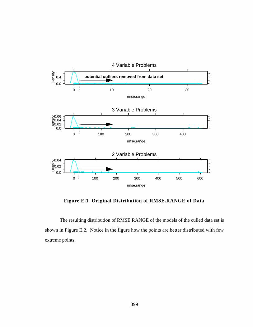
399
0.0
0.02
0.04
0 100 200 300 400 500 600
rmse.range
Den
sity
0.00.020.040.06
0 100 200 300 400
rmse.range
Den
sity
0.0
0.4
0 10 20 30
rmse.range
Den
sity
4 Variable Problems
3 Variable Problems
2 Variable Problems
potential outliers removed from data set
Figure E.1 Original Distribution of RMSE.RANGE of Data
The resulting distribution of RMSE.RANGE of the models of the culled data set is
shown in Figure E.2. Notice in the figure how the points are better distributed with few
extreme points.
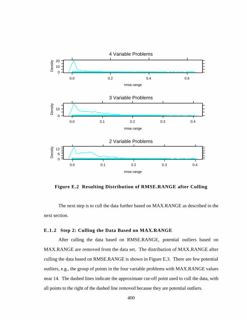
400
0
612
0.0 0.1 0.2 0.3 0.4
rmse.range
Den
sity
0
10
0.0 0.1 0.2 0.3 0.4
rmse.range
Den
sity
0
10
20
0.0 0.2 0.4 0.6
rmse.range
Den
sity
4 Variable Problems
3 Variable Problems
2 Variable Problems
Figure E.2 Resulting Distribution of RMSE.RANGE after Culling
The next step is to cull the data further based on MAX.RANGE as described in the
next section.
E.1.2 Step 2: Culling the Data Based on MAX.RANGE
After culling the data based on RMSE.RANGE, potential outliers based on
MAX.RANGE are removed from the data set. The distribution of MAX.RANGE after
culling the data based on RMSE.RANGE is shown in Figure E.3. There are few potential
outliers, e.g., the group of points in the four variable problems with MAX.RANGE values
near 14. The dashed lines indicate the approximate cut-off point used to cull the data, with
all points to the right of the dashed line removed because they are potential outliers.
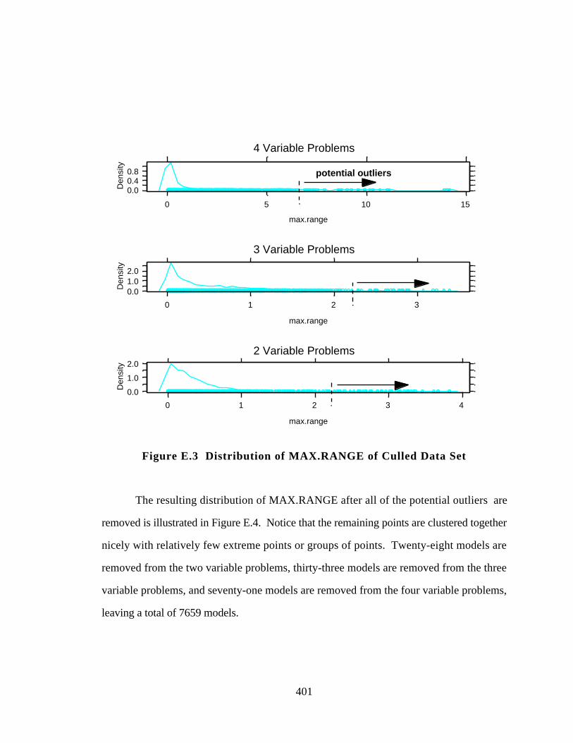
401
0.0
1.0
2.0
0 1 2 3 4
max.range
Den
sity
0.01.02.0
0 1 2 3
max.range
Den
sity
0.00.40.8
0 5 10 15
max.range
Den
sity
4 Variable Problems
3 Variable Problems
2 Variable Problems
potential outliers
Figure E.3 Distribution of MAX.RANGE of Culled Data Set
The resulting distribution of MAX.RANGE after all of the potential outliers are
removed is illustrated in Figure E.4. Notice that the remaining points are clustered together
nicely with relatively few extreme points or groups of points. Twenty-eight models are
removed from the two variable problems, thirty-three models are removed from the three
variable problems, and seventy-one models are removed from the four variable problems,
leaving a total of 7659 models.
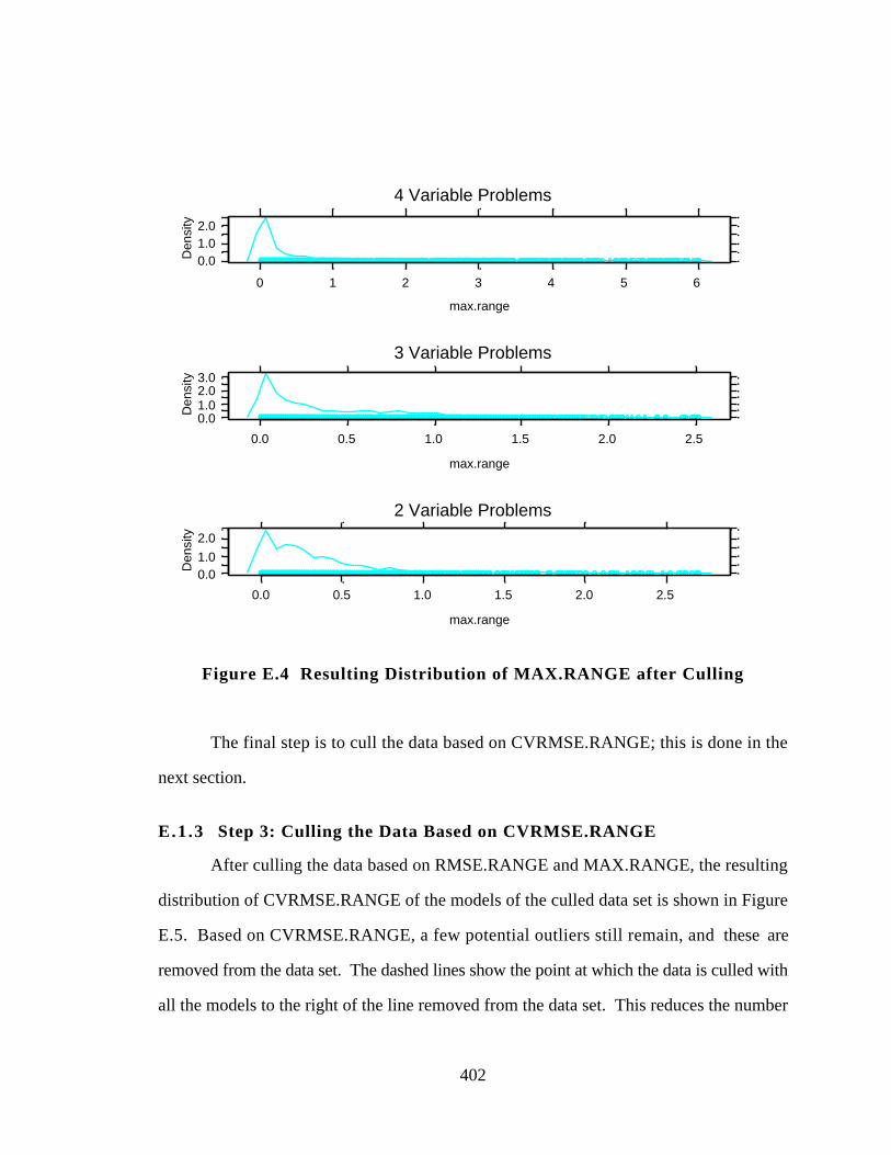
402
0.01.0
2.0
0.0 0.5 1.0 1.5 2.0 2.5
max.range
Den
sity
0.01.02.03.0
0.0 0.5 1.0 1.5 2.0 2.5
max.range
Den
sity
0.01.02.0
0 1 2 3 4 5 6
max.range
Den
sity
4 Variable Problems
3 Variable Problems
2 Variable Problems
Figure E.4 Resulting Distribution of MAX.RANGE after Culling
The final step is to cull the data based on CVRMSE.RANGE; this is done in the
next section.
E.1.3 Step 3: Culling the Data Based on CVRMSE.RANGE
After culling the data based on RMSE.RANGE and MAX.RANGE, the resulting
distribution of CVRMSE.RANGE of the models of the culled data set is shown in Figure
E.5. Based on CVRMSE.RANGE, a few potential outliers still remain, and these are
removed from the data set. The dashed lines show the point at which the data is culled with
all the models to the right of the line removed from the data set. This reduces the number
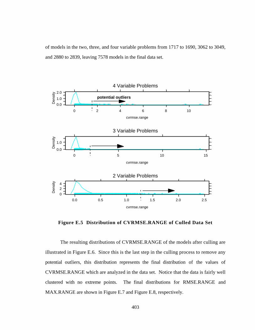
403
of models in the two, three, and four variable problems from 1717 to 1690, 3062 to 3049,
and 2880 to 2839, leaving 7578 models in the final data set.
0
24
0.0 0.5 1.0 1.5 2.0 2.5
cvrmse.range
Den
sity
0.0
1.0
0 5 10 15
cvrmse.range
Den
sity
0.0
1.0
2.0
0 2 4 6 8 10
cvrmse.range
Den
sity
4 Variable Problems
3 Variable Problems
2 Variable Problems
potential outliers
Figure E.5 Distribution of CVRMSE.RANGE of Culled Data Set
The resulting distributions of CVRMSE.RANGE of the models after culling are
illustrated in Figure E.6. Since this is the last step in the culling process to remove any
potential outliers, this distribution represents the final distribution of the values of
CVRMSE.RANGE which are analyzed in the data set. Notice that the data is fairly well
clustered with no extreme points. The final distributions for RMSE.RANGE and
MAX.RANGE are shown in Figure E.7 and Figure E.8, respectively.
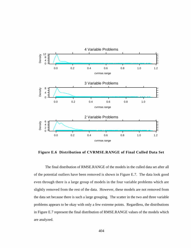
404
0246
0.0 0.2 0.4 0.6 0.8 1.0 1.2
cvrmse.range
Den
sity
0
4
8
0.0 0.2 0.4 0.6 0.8 1.0
cvrmse.range
Den
sity
048
12
0.0 0.2 0.4 0.6 0.8 1.0 1.2
cvrmse.range
Den
sity
4 Variable Problems
3 Variable Problems
2 Variable Problems
Figure E.6 Distribution of CVRMSE.RANGE of Final Culled Data Set
The final distribution of RMSE.RANGE of the models in the culled data set after all
of the potential outliers have been removed is shown in Figure E.7. The data look good
even through there is a large group of models in the four variable problems which are
slightly removed from the rest of the data. However, these models are not removed from
the data set because there is such a large grouping. The scatter in the two and three variable
problems appears to be okay with only a few extreme points. Regardless, the distributions
in Figure E.7 represent the final distribution of RMSE.RANGE values of the models which
are analyzed.
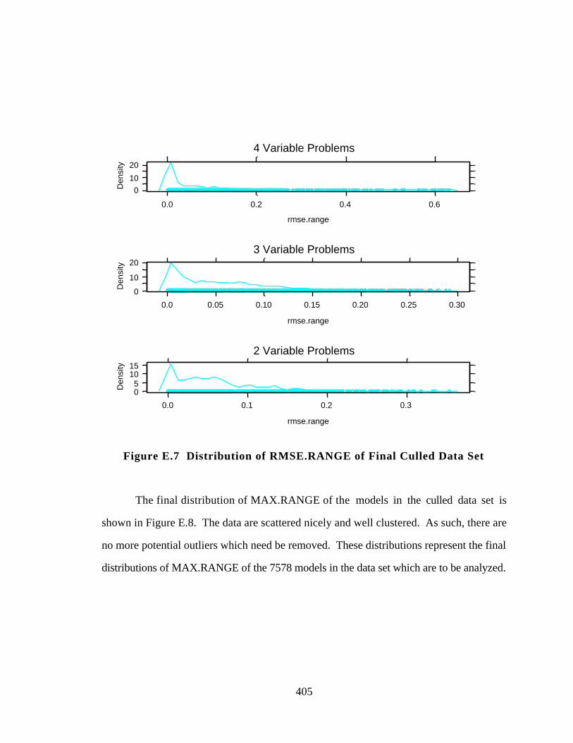
405
05
1015
0.0 0.1 0.2 0.3
rmse.range
Den
sity
0
10
20
0.0 0.05 0.10 0.15 0.20 0.25 0.30
rmse.range
Den
sity
0
10
20
0.0 0.2 0.4 0.6
rmse.range
Den
sity
4 Variable Problems
3 Variable Problems
2 Variable Problems
Figure E.7 Distribution of RMSE.RANGE of Final Culled Data Set
The final distribution of MAX.RANGE of the models in the culled data set is
shown in Figure E.8. The data are scattered nicely and well clustered. As such, there are
no more potential outliers which need be removed. These distributions represent the final
distributions of MAX.RANGE of the 7578 models in the data set which are to be analyzed.
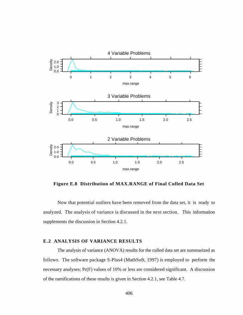
406
0.01.02.0
0.0 0.5 1.0 1.5 2.0 2.5
max.range
Den
sity
0123
0.0 0.5 1.0 1.5 2.0 2.5
max.range
Den
sity
0.01.02.0
0 1 2 3 4 5 6
max.range
Den
sity
4 Variable Problems
3 Variable Problems
2 Variable Problems
Figure E.8 Distribution of MAX.RANGE of Final Culled Data Set
Now that potential outliers have been removed from the data set, it is ready to
analyzed. The analysis of variance is discussed in the next section. This information
supplements the discussion in Section 4.2.1.
E.2 ANALYSIS OF VARIANCE RESULTS
The analysis of variance (ANOVA) results for the culled data set are summarized as
follows. The software package S-Plus4 (MathSoft, 1997) is employed to perform the
necessary analyses; Pr(F) values of 10% or less are considered significant. A discussion
of the ramifications of these results is given in Section 4.2.1, see Table 4.7.
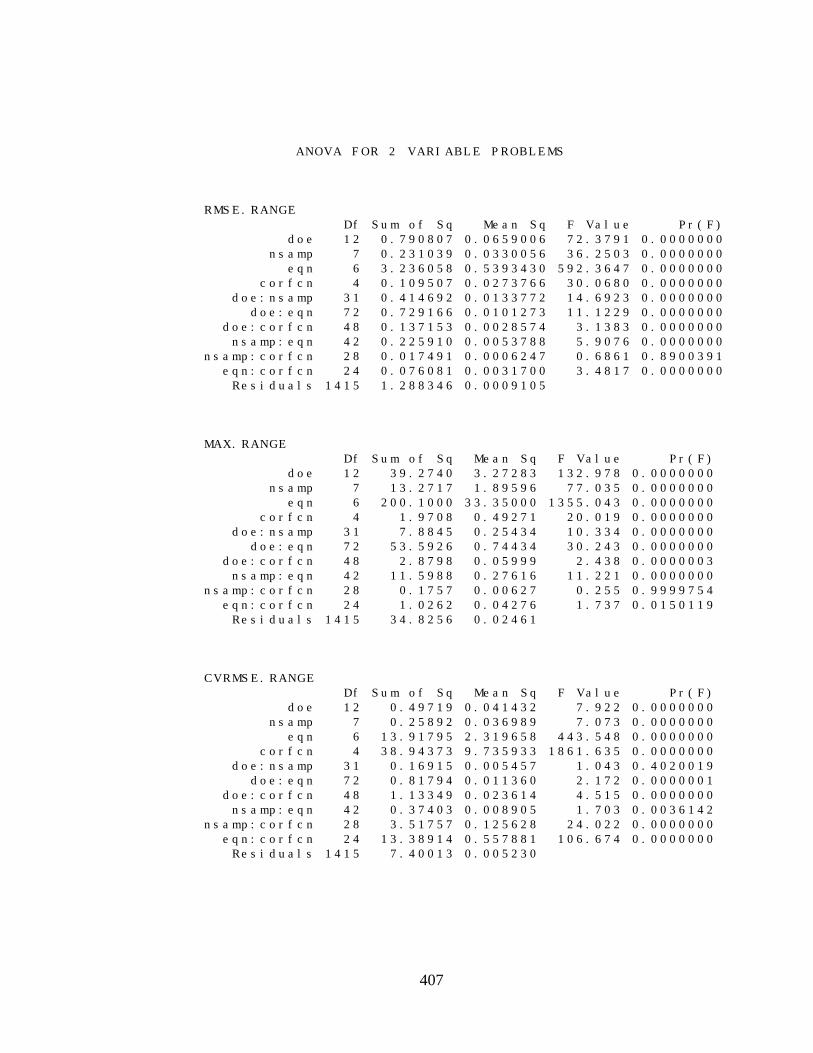
407
ANOVA FOR 2 VARIABLE PROBLEMS
RMSE.RANGE Df Sum of Sq Mean Sq F Value Pr(F) doe 12 0.790807 0.0659006 72.3791 0.0000000 nsamp 7 0.231039 0.0330056 36.2503 0.0000000 eqn 6 3.236058 0.5393430 592.3647 0.0000000 corfcn 4 0.109507 0.0273766 30.0680 0.0000000 doe:nsamp 31 0.414692 0.0133772 14.6923 0.0000000 doe:eqn 72 0.729166 0.0101273 11.1229 0.0000000 doe:corfcn 48 0.137153 0.0028574 3.1383 0.0000000 nsamp:eqn 42 0.225910 0.0053788 5.9076 0.0000000nsamp:corfcn 28 0.017491 0.0006247 0.6861 0.8900391 eqn:corfcn 24 0.076081 0.0031700 3.4817 0.0000000 Residuals 1415 1.288346 0.0009105
MAX.RANGE Df Sum of Sq Mean Sq F Value Pr(F) doe 12 39.2740 3.27283 132.978 0.0000000 nsamp 7 13.2717 1.89596 77.035 0.0000000 eqn 6 200.1000 33.35000 1355.043 0.0000000 corfcn 4 1.9708 0.49271 20.019 0.0000000 doe:nsamp 31 7.8845 0.25434 10.334 0.0000000 doe:eqn 72 53.5926 0.74434 30.243 0.0000000 doe:corfcn 48 2.8798 0.05999 2.438 0.0000003 nsamp:eqn 42 11.5988 0.27616 11.221 0.0000000nsamp:corfcn 28 0.1757 0.00627 0.255 0.9999754 eqn:corfcn 24 1.0262 0.04276 1.737 0.0150119 Residuals 1415 34.8256 0.02461
CVRMSE.RANGE Df Sum of Sq Mean Sq F Value Pr(F) doe 12 0.49719 0.041432 7.922 0.0000000 nsamp 7 0.25892 0.036989 7.073 0.0000000 eqn 6 13.91795 2.319658 443.548 0.0000000 corfcn 4 38.94373 9.735933 1861.635 0.0000000 doe:nsamp 31 0.16915 0.005457 1.043 0.4020019 doe:eqn 72 0.81794 0.011360 2.172 0.0000001 doe:corfcn 48 1.13349 0.023614 4.515 0.0000000 nsamp:eqn 42 0.37403 0.008905 1.703 0.0036142nsamp:corfcn 28 3.51757 0.125628 24.022 0.0000000 eqn:corfcn 24 13.38914 0.557881 106.674 0.0000000 Residuals 1415 7.40013 0.005230
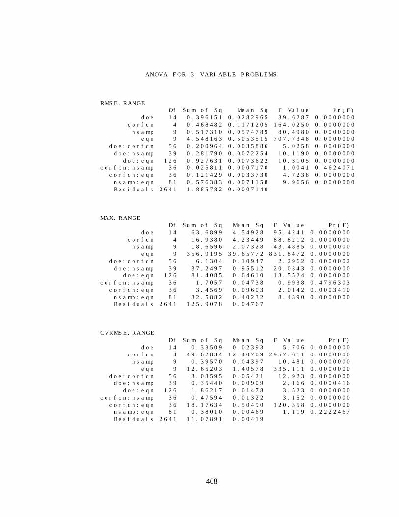
408
ANOVA FOR 3 VARIABLE PROBLEMS
RMSE.RANGE Df Sum of Sq Mean Sq F Value Pr(F) doe 14 0.396151 0.0282965 39.6287 0.0000000 corfcn 4 0.468482 0.1171205 164.0250 0.0000000 nsamp 9 0.517310 0.0574789 80.4980 0.0000000 eqn 9 4.548163 0.5053515 707.7348 0.0000000 doe:corfcn 56 0.200964 0.0035886 5.0258 0.0000000 doe:nsamp 39 0.281790 0.0072254 10.1190 0.0000000 doe:eqn 126 0.927631 0.0073622 10.3105 0.0000000corfcn:nsamp 36 0.025811 0.0007170 1.0041 0.4624071 corfcn:eqn 36 0.121429 0.0033730 4.7238 0.0000000 nsamp:eqn 81 0.576383 0.0071158 9.9656 0.0000000 Residuals 2641 1.885782 0.0007140
MAX.RANGE Df Sum of Sq Mean Sq F Value Pr(F) doe 14 63.6899 4.54928 95.4241 0.0000000 corfcn 4 16.9380 4.23449 88.8212 0.0000000 nsamp 9 18.6596 2.07328 43.4885 0.0000000 eqn 9 356.9195 39.65772 831.8472 0.0000000 doe:corfcn 56 6.1304 0.10947 2.2962 0.0000002 doe:nsamp 39 37.2497 0.95512 20.0343 0.0000000 doe:eqn 126 81.4085 0.64610 13.5524 0.0000000corfcn:nsamp 36 1.7057 0.04738 0.9938 0.4796303 corfcn:eqn 36 3.4569 0.09603 2.0142 0.0003410 nsamp:eqn 81 32.5882 0.40232 8.4390 0.0000000 Residuals 2641 125.9078 0.04767
CVRMSE.RANGE Df Sum of Sq Mean Sq F Value Pr(F) doe 14 0.33509 0.02393 5.706 0.0000000 corfcn 4 49.62834 12.40709 2957.611 0.0000000 nsamp 9 0.39570 0.04397 10.481 0.0000000 eqn 9 12.65203 1.40578 335.111 0.0000000 doe:corfcn 56 3.03595 0.05421 12.923 0.0000000 doe:nsamp 39 0.35440 0.00909 2.166 0.0000416 doe:eqn 126 1.86217 0.01478 3.523 0.0000000corfcn:nsamp 36 0.47594 0.01322 3.152 0.0000000 corfcn:eqn 36 18.17634 0.50490 120.358 0.0000000 nsamp:eqn 81 0.38010 0.00469 1.119 0.2222467 Residuals 2641 11.07891 0.00419
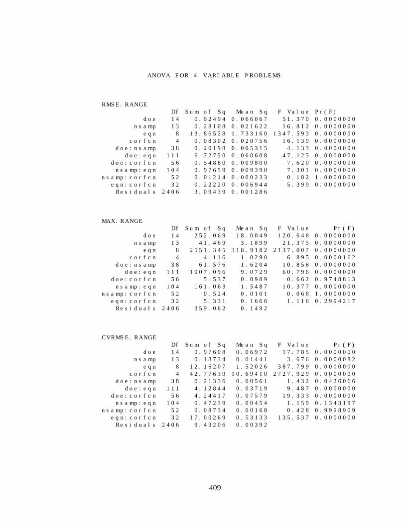
409
ANOVA FOR 4 VARIABLE PROBLEMS
RMSE.RANGE Df Sum of Sq Mean Sq F Value Pr(F) doe 14 0.92494 0.066067 51.370 0.0000000 nsamp 13 0.28108 0.021622 16.812 0.0000000 eqn 8 13.86528 1.733160 1347.593 0.0000000 corfcn 4 0.08302 0.020756 16.139 0.0000000 doe:nsamp 38 0.20198 0.005315 4.133 0.0000000 doe:eqn 111 6.72750 0.060608 47.125 0.0000000 doe:corfcn 56 0.54880 0.009800 7.620 0.0000000 nsamp:eqn 104 0.97659 0.009390 7.301 0.0000000nsamp:corfcn 52 0.01214 0.000233 0.182 1.0000000 eqn:corfcn 32 0.22220 0.006944 5.399 0.0000000 Residuals 2406 3.09439 0.001286
MAX.RANGE Df Sum of Sq Mean Sq F Value Pr(F) doe 14 252.069 18.0049 120.648 0.0000000 nsamp 13 41.469 3.1899 21.375 0.0000000 eqn 8 2551.345 318.9182 2137.007 0.0000000 corfcn 4 4.116 1.0290 6.895 0.0000162 doe:nsamp 38 61.576 1.6204 10.858 0.0000000 doe:eqn 111 1007.096 9.0729 60.796 0.0000000 doe:corfcn 56 5.537 0.0989 0.662 0.9748813 nsamp:eqn 104 161.063 1.5487 10.377 0.0000000nsamp:corfcn 52 0.524 0.0101 0.068 1.0000000 eqn:corfcn 32 5.331 0.1666 1.116 0.2994217 Residuals 2406 359.062 0.1492
CVRMSE.RANGE Df Sum of Sq Mean Sq F Value Pr(F) doe 14 0.97608 0.06972 17.785 0.0000000 nsamp 13 0.18734 0.01441 3.676 0.0000082 eqn 8 12.16207 1.52026 387.799 0.0000000 corfcn 4 42.77639 10.69410 2727.929 0.0000000 doe:nsamp 38 0.21336 0.00561 1.432 0.0426066 doe:eqn 111 4.12844 0.03719 9.487 0.0000000 doe:corfcn 56 4.24417 0.07579 19.333 0.0000000 nsamp:eqn 104 0.47239 0.00454 1.159 0.1343197nsamp:corfcn 52 0.08734 0.00168 0.428 0.9998909 eqn:corfcn 32 17.00269 0.53133 135.537 0.0000000 Residuals 2406 9.43206 0.00392
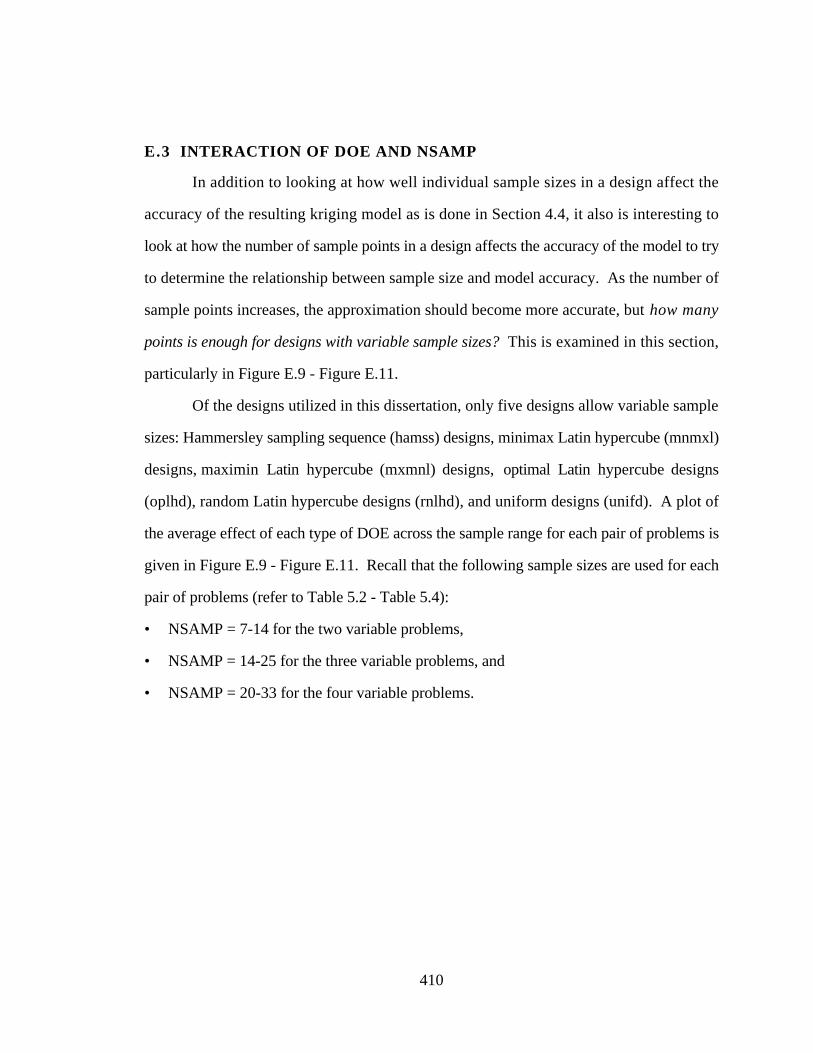
410
E.3 INTERACTION OF DOE AND NSAMP
In addition to looking at how well individual sample sizes in a design affect the
accuracy of the resulting kriging model as is done in Section 4.4, it also is interesting to
look at how the number of sample points in a design affects the accuracy of the model to try
to determine the relationship between sample size and model accuracy. As the number of
sample points increases, the approximation should become more accurate, but how many
points is enough for designs with variable sample sizes? This is examined in this section,
particularly in Figure E.9 - Figure E.11.
Of the designs utilized in this dissertation, only five designs allow variable sample
sizes: Hammersley sampling sequence (hamss) designs, minimax Latin hypercube (mnmxl)
designs, maximin Latin hypercube (mxmnl) designs, optimal Latin hypercube designs
(oplhd), random Latin hypercube designs (rnlhd), and uniform designs (unifd). A plot of
the average effect of each type of DOE across the sample range for each pair of problems is
given in Figure E.9 - Figure E.11. Recall that the following sample sizes are used for each
pair of problems (refer to Table 5.2 - Table 5.4):
• NSAMP = 7-14 for the two variable problems,
• NSAMP = 14-25 for the three variable problems, and
• NSAMP = 20-33 for the four variable problems.
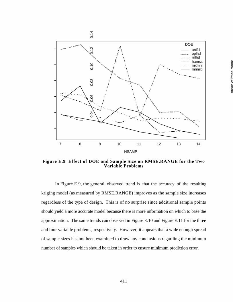
411
NSAMP
mea
n of
rm
se.r
ange
0.04
0.06
0.08
0.10
0.12
0.14
7 8 9 10 11 12 13 14
DOEunifdoplhdrnlhdhamssmxmnlmnmxl
Figure E.9 Effect of DOE and Sample Size on RMSE.RANGE for the TwoVariable Problems
In Figure E.9, the general observed trend is that the accuracy of the resulting
kriging model (as measured by RMSE.RANGE) improves as the sample size increases
regardless of the type of design. This is of no surprise since additional sample points
should yield a more accurate model because there is more information on which to base the
approximation. The same trends can observed in Figure E.10 and Figure E.11 for the three
and four variable problems, respectively. However, it appears that a wide enough spread
of sample sizes has not been examined to draw any conclusions regarding the minimum
number of samples which should be taken in order to ensure minimum prediction error.
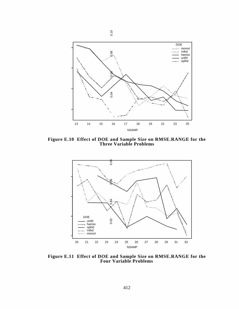
412
0.04
0.06
0.08
0.10
13 14 15 16 17 18 19 21 23 25
mnmxlrnlhdhamssunifdoplhd
DOE
NSAMP
mea
n of
rm
se.r
ange
Figure E.10 Effect of DOE and Sample Size on RMSE.RANGE for theThree Variable Problems
NSAMP
mea
n of
rm
se.r
ange
0.02
0.04
0.06
0.08
20 21 22 23 24 25 26 27 28 29 31 33
DOEunifdhamssoplhdrnlhdmnmxl
Figure E.11 Effect of DOE and Sample Size on RMSE.RANGE for theFour Variable Problems
413
F. APPENDIX F
SUPPLEMENTAL INFORMATION FOR GAAEXAMPLE PROBLEM
This appendix contains detailed supplemental information for the GAA example
problem in Chapter 7. Section F.1 contains a brief description of the design variables used
in the GAA example. The sample points, data, and MLE theta parameters for the kriging
metamodels are given in Section F.2. Analysis of variance of the sample data is offered in
Section F.3; it is used to generate the Pareto plots in Section 7.6.3. Additional design
scenarios for the exercising the PPCEM product platform compromise DSP are presented
and discussed in Section F.4, and convergence histories for the individually designed
benchmark aircraft for Scenarios 1-3 are plotted in Section F.5. Information for the GAA
product variety tradeoff study discussed in Section 7.6.3 is included in Section F.6.
Justification of the design variable weights used in the computation of NCI are explained in
Section F.6.1 while Sections F.6.2 and F.6.3 contain all of the results—instantiations of
each aircraft, responses, and corresponding deviation function values—of the product
variety tradeoff study for Scenarios 2 and 3, respectively. Finally, sample DSIDES files
for the PPCEM platform and the individual aircraft are included in Sections F.7 and F.8.
414
F.1 GAA DESIGN VARIABLE DESCRIPTION
The intent in this section is to provide the reader with a brief description of the
design variables considered in the GAA example—cruise speed, aspect ratio, propeller
diameter, wing loading, engine activity factor, and seat width—and why they are important
in aircraft design. Where applicable, typical ranges of the design variables for current GAA
are provide to justify the design variable bounds employed in this work.
Cruise speed (CSPD): General Aviation aircraft are typically subsonic aircraft with
cruise speed in the range of 0 < M < 0.6 where M is the mach number. Based on
the GAA Design Competition guidelines (NASA and FAA, 1994) the aircraft
should be capable of maintaining a cruise speed, CSPD, between 150 and 300 kts.
Therefore, the cruise speed Mach number varies from Mach 0.24 to Mach 0.48 in
order to find the “best” velocity at which to fly the cruise portion of the mission.
Aspect ratio (AR): Aspect ratio of a wing is defined as the span of the wing squared
divided by its area; span is the distance from wing tip to wing tip measured
perpendicular to the plane (Raymer, 1992). Raymer states that the Wright brothers
were the first to investigate the effect of aspect ratio on flight performance,
observing that a long, skinny wing (high aspect ratio) has less drag than a short, fat
wing (low aspect ratio). In general, wings with a high aspect ratio tend to have
lower induced drag and therefore larger values of (L/D)max. Moreover, a high
aspect ratio wing tends to have high lift-curve slopes. High lift curve slopes have
two consequences:
1. at low speeds, the approach attitude is conducive to good runway visibility from
the cockpit, and
2. the ride through turbulence is rougher.
Also, high aspect ratio wings usually weigh more than low aspect ratio wings. In
general, General aviation aircraft have aspect ratios ranging from 7.6 (single
engine) to 9.2 (twin turboprop). In this investigation, aspect ratios ranging from 7-
11 are investigated.
415
Propeller diameter (DPRP): Propeller diameter is self-explanatory. Generally
speaking, the larger the propeller diameter, the more efficient the propeller will be;
however, the limitation on the length of propeller diameter is the propeller tip speed
which should be kept below sonic speed (Raymer, 1992). From a survey of
modern GAA, the propeller diameter varies from 5.5 ft to 6.8 ft. Raymer suggests
to limit the tipspeed to be less than 850 ft/sec for wooden propellers; this translates
into a maximum diameter of 5.96 ft. A range of 5 ft to 5.96 ft is examined in this
problem.
Wing loading (WL): Wing loading is the ratio of the aircraft weight to the area of
the wing and affects stall speed, climb rate, takeoff and landing distances, and turn
performance; wing loading also has a very strong effect upon the takeoff gross
weight of an aircraft (Raymer, 1992). The larger the wing, the lower the wing
loading. Raymer notes that the larger wing helps reduce takeoff/landing field
lengths; however, the additional drag and empty weight due to the larger wing will
increase takeoff gross weight in order to perform the mission. A larger wing also is
liable to affect operating costs because more fuel is consumed to provide the
necessary lift to achieve the mission. Representative wing loadings of General
Aviation aircraft vary between 17 (single engine) and 26 (twin engine); the range
utilized in the GAA example is 17 to 25.
For the GAA flight envelope, i.e., cruise speeds of Mach 0.2 to Mach 0.6, piston
and turboprop engines are the most widely used engines. In addition, a piston engine has a
low fuel consumption compared to a turboprop engine. Although, the engine weight of a
piston engine (1.1 - 1.75 lb/take-off hp) is heavier than a turboprop (.35 - .55 lb/take-off
hp), the acquisition cost of the piston engine ($25 - $ 50/hp) is much cheaper than the
turboprop engine ($60 - $100/hp). General Aviation aircraft pilots are primarily concerned
about the direct operating cost (DOC) of the aircraft. In general practice, piston engines are
very competitive for GAA which require less than 500 hp compared to turboprop engines
which are more suitable for a powerful GAA engine of more than 500 hp. For this work,
the engine selected for the GAA design is a piston, reciprocate fuel injection, engine
equipped with 350 hp.

416
Engine activity factor (AF): To help size the engine, the engine activity factor is
used; it is a measure of the amount of power being absorbed by the propeller
(Raymer, 1992). Raymer states that engine activity factors range from about 90 -
200. For example, a typical light-aircraft, such as a general aviation aircraft, has an
activity factor of 100. A range of 85-110 is examined in this study where 110 is the
value of the baseline design.
Seat width (WS): The seat width is used to size the width of the cabin; in particular:
cabin width = 2 x (seat width) + (aisle width) + 12 in [A.1]
where aisle width is taken as a fixed parameter and 12 in. is the total thickness of
the fuselage walls. As seat width increases, cabin width increases and the surface
area of the fuselage increases causing an increased drag. Seat widths for an
economy sized aircraft vary between 17 in and 22 in, whereas seat widths in a small
aircraft vary between 16 in and 18 in (Raymer, 1992). In this study, the baseline
value of 20 in is used as the upper bound for seat width while the lower bound is
taken as 14 in for comfort reasons.
These six variables constitute the control factors for the General Aviation aircraft
family. The bounds on the design variables define the design space in which the kriging
models are constructed. The kriging model construction is documented in the next section.
F.2 GAA KRIGING METAMODELS: SAMPLE POINTS, RESPONSEVALUES, AND FITTED MLE PARAMETERS
Table F.1 contains the 64 sample points from the randomized orthogonal array used
in this study, and are scaled to fit the design space based on the bounds listed in the
beginning of Section 7.2. GASP is invoked using these 64 points for each aircraft; the
response values are listed in Table F.2 for the one passenger (two seater) aircraft, in Table
F.3 for the three passenger (four seater) aircraft, and in Table F.4 for the five passenger
(six seater) aircraft.
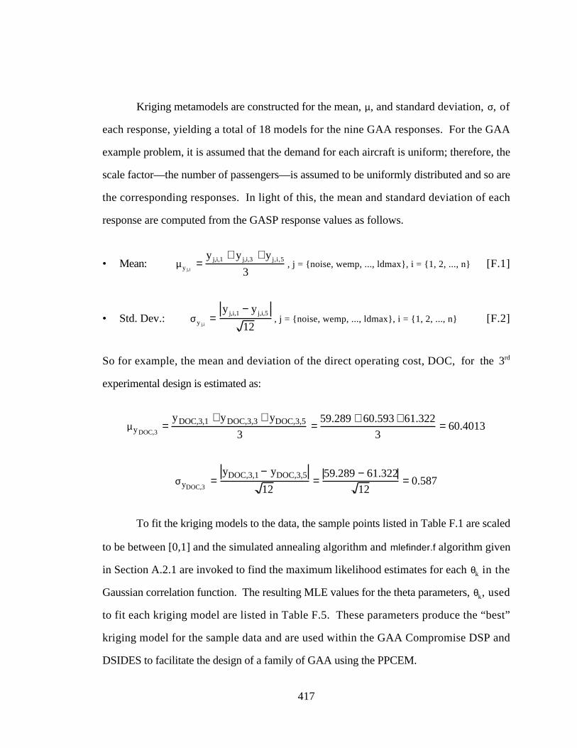
417
Kriging metamodels are constructed for the mean, µ, and standard deviation, σ, of
each response, yielding a total of 18 models for the nine GAA responses. For the GAA
example problem, it is assumed that the demand for each aircraft is uniform; therefore, the
scale factor—the number of passengers—is assumed to be uniformly distributed and so are
the corresponding responses. In light of this, the mean and standard deviation of each
response are computed from the GASP response values as follows.
• Mean: µy j,i=
y j,i,1 + y j,i,3 + y j,i,5
3, j = {noise, wemp, ..., ldmax}, i = {1, 2, ..., n} [F.1]
• Std. Dev.: σy j,i=
y j,i,1 − y j,i,5
12, j = {noise, wemp, ..., ldmax}, i = {1, 2, ..., n} [F.2]
So for example, the mean and deviation of the direct operating cost, DOC, for the 3rd
experimental design is estimated as:
µyDOC,3=
yDOC,3,1 + yDOC,3,3 + yDOC,3,5
3=
59.289 + 60.593 + 61.322
3= 60.4013
σyDOC,3=
yDOC,3,1 − yDOC,3,5
12=
59.289 − 61.322
12= 0.587
To fit the kriging models to the data, the sample points listed in Table F.1 are scaled
to be between [0,1] and the simulated annealing algorithm and mlefinder.f algorithm given
in Section A.2.1 are invoked to find the maximum likelihood estimates for each θk in the
Gaussian correlation function. The resulting MLE values for the theta parameters, θk, used
to fit each kriging model are listed in Table F.5. These parameters produce the “best”
kriging model for the sample data and are used within the GAA Compromise DSP and
DSIDES to facilitate the design of a family of GAA using the PPCEM.
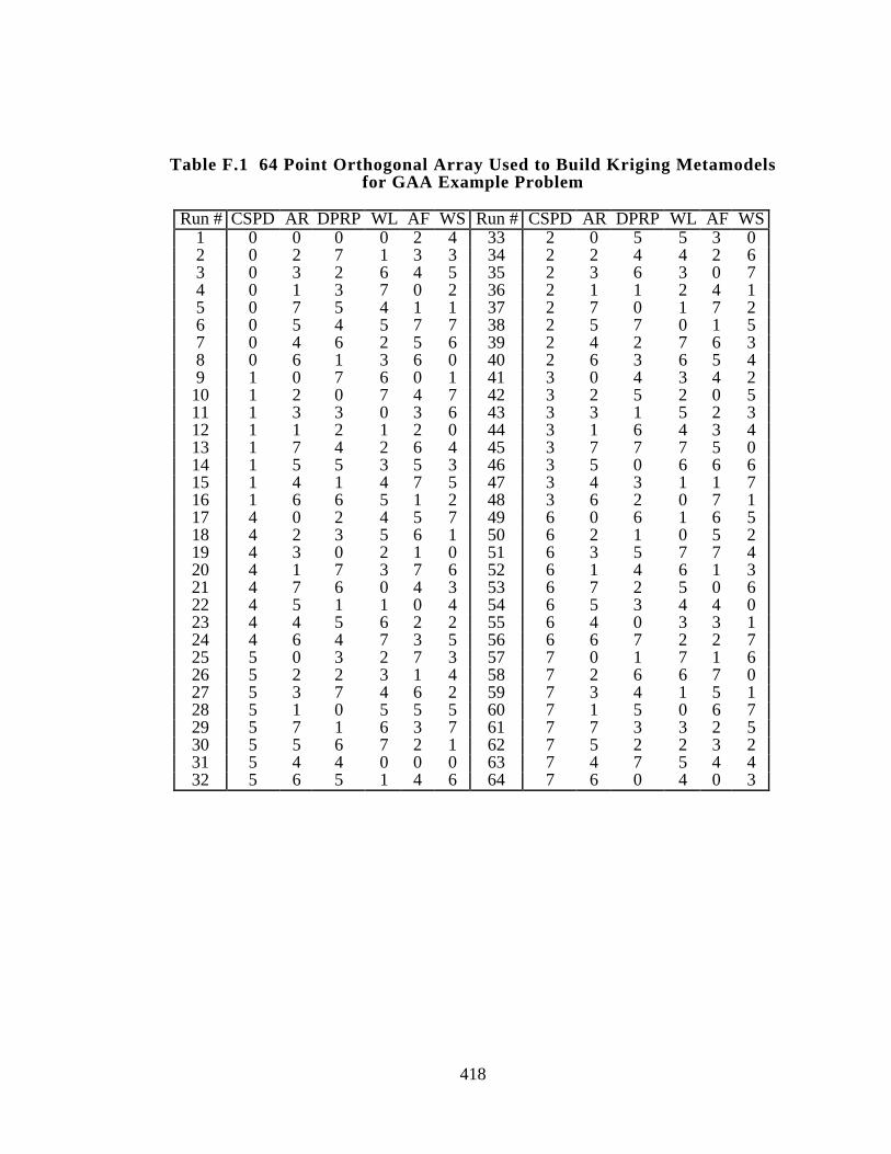
418
Table F.1 64 Point Orthogonal Array Used to Build Kriging Metamodelsfor GAA Example Problem
Run # CSPD AR DPRP WL AF WS Run # CSPD AR DPRP WL AF WS1 0 0 0 0 2 4 33 2 0 5 5 3 02 0 2 7 1 3 3 34 2 2 4 4 2 63 0 3 2 6 4 5 35 2 3 6 3 0 74 0 1 3 7 0 2 36 2 1 1 2 4 15 0 7 5 4 1 1 37 2 7 0 1 7 26 0 5 4 5 7 7 38 2 5 7 0 1 57 0 4 6 2 5 6 39 2 4 2 7 6 38 0 6 1 3 6 0 40 2 6 3 6 5 49 1 0 7 6 0 1 41 3 0 4 3 4 210 1 2 0 7 4 7 42 3 2 5 2 0 511 1 3 3 0 3 6 43 3 3 1 5 2 312 1 1 2 1 2 0 44 3 1 6 4 3 413 1 7 4 2 6 4 45 3 7 7 7 5 014 1 5 5 3 5 3 46 3 5 0 6 6 615 1 4 1 4 7 5 47 3 4 3 1 1 716 1 6 6 5 1 2 48 3 6 2 0 7 117 4 0 2 4 5 7 49 6 0 6 1 6 518 4 2 3 5 6 1 50 6 2 1 0 5 219 4 3 0 2 1 0 51 6 3 5 7 7 420 4 1 7 3 7 6 52 6 1 4 6 1 321 4 7 6 0 4 3 53 6 7 2 5 0 622 4 5 1 1 0 4 54 6 5 3 4 4 023 4 4 5 6 2 2 55 6 4 0 3 3 124 4 6 4 7 3 5 56 6 6 7 2 2 725 5 0 3 2 7 3 57 7 0 1 7 1 626 5 2 2 3 1 4 58 7 2 6 6 7 027 5 3 7 4 6 2 59 7 3 4 1 5 128 5 1 0 5 5 5 60 7 1 5 0 6 729 5 7 1 6 3 7 61 7 7 3 3 2 530 5 5 6 7 2 1 62 7 5 2 2 3 231 5 4 4 0 0 0 63 7 4 7 5 4 432 5 6 5 1 4 6 64 7 6 0 4 0 3
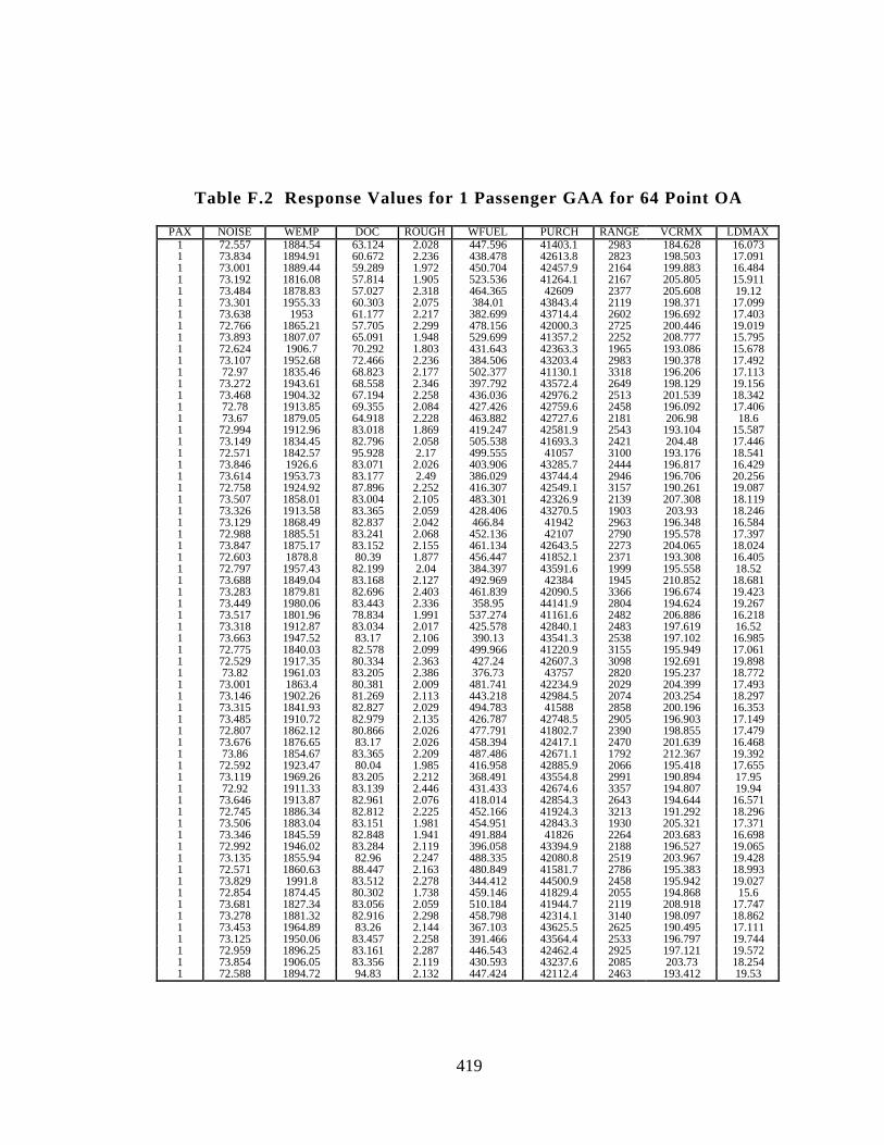
419
Table F.2 Response Values for 1 Passenger GAA for 64 Point OA
PAX NOISE WEMP DOC ROUGH WFUEL PURCH RANGE VCRMX LDMAX1 72.557 1884.54 63.124 2.028 447.596 41403.1 2983 184.628 16.0731 73.834 1894.91 60.672 2.236 438.478 42613.8 2823 198.503 17.0911 73.001 1889.44 59.289 1.972 450.704 42457.9 2164 199.883 16.4841 73.192 1816.08 57.814 1.905 523.536 41264.1 2167 205.805 15.9111 73.484 1878.83 57.027 2.318 464.365 42609 2377 205.608 19.121 73.301 1955.33 60.303 2.075 384.01 43843.4 2119 198.371 17.0991 73.638 1953 61.177 2.217 382.699 43714.4 2602 196.692 17.4031 72.766 1865.21 57.705 2.299 478.156 42000.3 2725 200.446 19.0191 73.893 1807.07 65.091 1.948 529.699 41357.2 2252 208.777 15.7951 72.624 1906.7 70.292 1.803 431.643 42363.3 1965 193.086 15.6781 73.107 1952.68 72.466 2.236 384.506 43203.4 2983 190.378 17.4921 72.97 1835.46 68.823 2.177 502.377 41130.1 3318 196.206 17.1131 73.272 1943.61 68.558 2.346 397.792 43572.4 2649 198.129 19.1561 73.468 1904.32 67.194 2.258 436.036 42976.2 2513 201.539 18.3421 72.78 1913.85 69.355 2.084 427.426 42759.6 2458 196.092 17.4061 73.67 1879.05 64.918 2.228 463.882 42727.6 2181 206.98 18.61 72.994 1912.96 83.018 1.869 419.247 42581.9 2543 193.104 15.5871 73.149 1834.45 82.796 2.058 505.538 41693.3 2421 204.48 17.4461 72.571 1842.57 95.928 2.17 499.555 41057 3100 193.176 18.5411 73.846 1926.6 83.071 2.026 403.906 43285.7 2444 196.817 16.4291 73.614 1953.73 83.177 2.49 386.029 43744.4 2946 196.706 20.2561 72.758 1924.92 87.896 2.252 416.307 42549.1 3157 190.261 19.0871 73.507 1858.01 83.004 2.105 483.301 42326.9 2139 207.308 18.1191 73.326 1913.58 83.365 2.059 428.406 43270.5 1903 203.93 18.2461 73.129 1868.49 82.837 2.042 466.84 41942 2963 196.348 16.5841 72.988 1885.51 83.241 2.068 452.136 42107 2790 195.578 17.3971 73.847 1875.17 83.152 2.155 461.134 42643.5 2273 204.065 18.0241 72.603 1878.8 80.39 1.877 456.447 41852.1 2371 193.308 16.4051 72.797 1957.43 82.199 2.04 384.397 43591.6 1999 195.558 18.521 73.688 1849.04 83.168 2.127 492.969 42384 1945 210.852 18.6811 73.283 1879.81 82.696 2.403 461.839 42090.5 3366 196.674 19.4231 73.449 1980.06 83.443 2.336 358.95 44141.9 2804 194.624 19.2671 73.517 1801.96 78.834 1.991 537.274 41161.6 2482 206.886 16.2181 73.318 1912.87 83.034 2.017 425.578 42840.1 2483 197.619 16.521 73.663 1947.52 83.17 2.106 390.13 43541.3 2538 197.102 16.9851 72.775 1840.03 82.578 2.099 499.966 41220.9 3155 195.949 17.0611 72.529 1917.35 80.334 2.363 427.24 42607.3 3098 192.691 19.8981 73.82 1961.03 83.205 2.386 376.73 43757 2820 195.237 18.7721 73.001 1863.4 80.381 2.009 481.741 42234.9 2029 204.399 17.4931 73.146 1902.26 81.269 2.113 443.218 42984.5 2074 203.254 18.2971 73.315 1841.93 82.827 2.029 494.783 41588 2858 200.196 16.3531 73.485 1910.72 82.979 2.135 426.787 42748.5 2905 196.903 17.1491 72.807 1862.12 80.866 2.026 477.791 41802.7 2390 198.855 17.4791 73.676 1876.65 83.17 2.026 458.394 42417.1 2470 201.639 16.4681 73.86 1854.67 83.365 2.209 487.486 42671.1 1792 212.367 19.3921 72.592 1923.47 80.04 1.985 416.958 42885.9 2066 195.418 17.6551 73.119 1969.26 83.205 2.212 368.491 43554.8 2991 190.894 17.951 72.92 1911.33 83.139 2.446 431.433 42674.6 3357 194.807 19.941 73.646 1913.87 82.961 2.076 418.014 42854.3 2643 194.644 16.5711 72.745 1886.34 82.812 2.225 452.166 41924.3 3213 191.292 18.2961 73.506 1883.04 83.151 1.981 454.951 42843.3 1930 205.321 17.3711 73.346 1845.59 82.848 1.941 491.884 41826 2264 203.683 16.6981 72.992 1946.02 83.284 2.119 396.058 43394.9 2188 196.527 19.0651 73.135 1855.94 82.96 2.247 488.335 42080.8 2519 203.967 19.4281 72.571 1860.63 88.447 2.163 480.849 41581.7 2786 195.383 18.9931 73.829 1991.8 83.512 2.278 344.412 44500.9 2458 195.942 19.0271 72.854 1874.45 80.302 1.738 459.146 41829.4 2055 194.868 15.61 73.681 1827.34 83.056 2.059 510.184 41944.7 2119 208.918 17.7471 73.278 1881.32 82.916 2.298 458.798 42314.1 3140 198.097 18.8621 73.453 1964.89 83.26 2.144 367.103 43625.5 2625 190.495 17.1111 73.125 1950.06 83.457 2.258 391.466 43564.4 2533 196.797 19.7441 72.959 1896.25 83.161 2.287 446.543 42462.4 2925 197.121 19.5721 73.854 1906.05 83.356 2.119 430.593 43237.6 2085 203.73 18.2541 72.588 1894.72 94.83 2.132 447.424 42112.4 2463 193.412 19.53
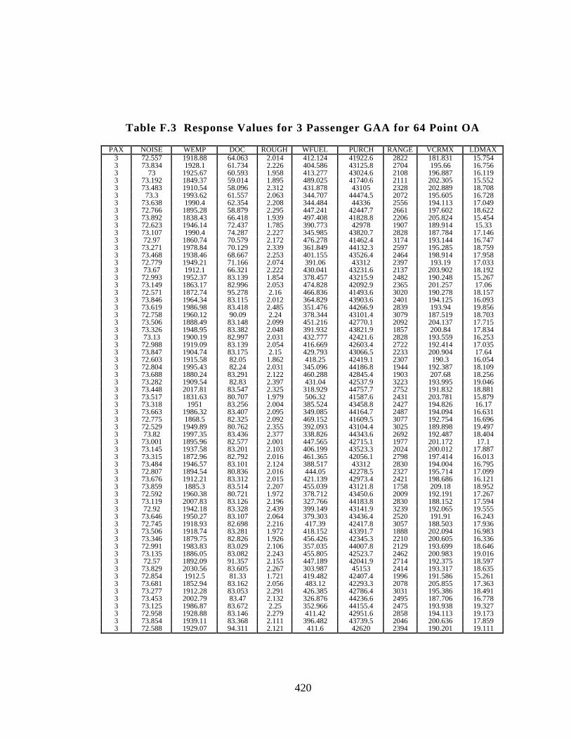
420
Table F.3 Response Values for 3 Passenger GAA for 64 Point OA
PAX NOISE WEMP DOC ROUGH WFUEL PURCH RANGE VCRMX LDMAX3 72.557 1918.88 64.063 2.014 412.124 41922.6 2822 181.831 15.7543 73.834 1928.1 61.734 2.226 404.586 43125.8 2704 195.66 16.7563 73 1925.67 60.593 1.958 413.277 43024.6 2108 196.887 16.1193 73.192 1849.37 59.014 1.895 489.025 41740.6 2111 202.305 15.5523 73.483 1910.54 58.096 2.312 431.878 43105 2328 202.889 18.7083 73.3 1993.62 61.557 2.063 344.707 44474.5 2072 195.605 16.7283 73.638 1990.4 62.354 2.208 344.484 44336 2556 194.113 17.0493 72.766 1895.28 58.879 2.295 447.241 42447.7 2661 197.602 18.6223 73.892 1838.43 66.418 1.939 497.408 41828.8 2206 205.824 15.4543 72.623 1946.14 72.437 1.785 390.773 42978 1907 189.914 15.333 73.107 1990.4 74.287 2.227 345.985 43820.7 2828 187.784 17.1463 72.97 1860.74 70.579 2.172 476.278 41462.4 3174 193.144 16.7473 73.271 1978.84 70.129 2.339 361.849 44132.3 2597 195.285 18.7593 73.468 1938.46 68.667 2.253 401.155 43526.4 2464 198.914 17.9583 72.779 1949.21 71.166 2.074 391.06 43312 2397 193.19 17.0333 73.67 1912.1 66.321 2.222 430.041 43231.6 2137 203.902 18.1923 72.993 1952.37 83.139 1.854 378.457 43215.9 2482 190.248 15.2673 73.149 1863.17 82.996 2.053 474.828 42092.9 2365 201.257 17.063 72.571 1872.74 95.278 2.16 466.836 41493.6 3020 190.278 18.1573 73.846 1964.34 83.115 2.012 364.829 43903.6 2401 194.125 16.0933 73.619 1986.98 83.418 2.485 351.476 44266.9 2839 193.94 19.8563 72.758 1960.12 90.09 2.24 378.344 43101.4 3079 187.519 18.7033 73.506 1888.49 83.148 2.099 451.216 42770.1 2092 204.137 17.7153 73.326 1948.95 83.382 2.048 391.932 43821.9 1857 200.84 17.8343 73.13 1900.19 82.997 2.031 432.777 42421.6 2828 193.559 16.2533 72.988 1919.09 83.139 2.054 416.669 42603.4 2722 192.414 17.0353 73.847 1904.74 83.175 2.15 429.793 43066.5 2233 200.904 17.643 72.603 1915.58 82.05 1.862 418.25 42419.1 2307 190.3 16.0543 72.804 1995.43 82.24 2.031 345.096 44186.8 1944 192.387 18.1093 73.688 1880.24 83.291 2.122 460.288 42845.4 1903 207.68 18.2563 73.282 1909.54 82.83 2.397 431.04 42537.9 3223 193.995 19.0463 73.448 2017.81 83.547 2.325 318.929 44757.7 2752 191.832 18.8813 73.517 1831.63 80.707 1.979 506.32 41587.6 2431 203.781 15.8793 73.318 1951 83.256 2.004 385.524 43458.8 2427 194.826 16.173 73.663 1986.32 83.407 2.095 349.085 44164.7 2487 194.094 16.6313 72.775 1868.5 82.325 2.092 469.152 41609.5 3077 192.754 16.6963 72.529 1949.89 80.762 2.355 392.093 43104.4 3025 189.898 19.4973 73.82 1997.35 83.436 2.377 338.826 44343.6 2692 192.487 18.4043 73.001 1895.96 82.577 2.001 447.565 42715.1 1977 201.172 17.13 73.145 1937.58 83.201 2.103 406.199 43523.3 2024 200.012 17.8873 73.315 1872.96 82.792 2.016 461.365 42056.1 2798 197.414 16.0133 73.484 1946.57 83.101 2.124 388.517 43312 2830 194.004 16.7953 72.807 1894.54 80.836 2.016 444.05 42278.5 2327 195.714 17.0993 73.676 1912.21 83.312 2.015 421.139 42973.4 2421 198.686 16.1213 73.859 1885.3 83.514 2.207 455.039 43121.8 1758 209.18 18.9523 72.592 1960.38 80.721 1.972 378.712 43450.6 2009 192.191 17.2673 73.119 2007.83 83.126 2.196 327.766 44183.8 2830 188.152 17.5943 72.92 1942.18 83.328 2.439 399.149 43141.9 3239 192.065 19.5553 73.646 1950.27 83.107 2.064 379.303 43436.4 2520 191.91 16.2433 72.745 1918.93 82.698 2.216 417.39 42417.8 3057 188.503 17.9363 73.506 1918.74 83.281 1.972 418.152 43391.7 1888 202.094 16.9833 73.346 1879.75 82.826 1.926 456.426 42345.3 2210 200.605 16.3363 72.991 1983.83 83.029 2.106 357.035 44007.8 2129 193.699 18.6463 73.135 1886.05 83.082 2.243 455.805 42523.7 2462 200.983 19.0163 72.57 1892.09 91.357 2.155 447.189 42041.9 2714 192.375 18.5973 73.829 2030.56 83.605 2.267 303.987 45153 2414 193.317 18.6353 72.854 1912.5 81.33 1.721 419.482 42407.4 1996 191.586 15.2613 73.681 1852.94 83.162 2.056 483.12 42293.3 2078 205.855 17.3633 73.277 1912.28 83.053 2.291 426.385 42786.4 3031 195.386 18.4913 73.453 2002.79 83.47 2.132 326.876 44236.6 2495 187.706 16.7783 73.125 1986.87 83.672 2.25 352.966 44155.4 2475 193.938 19.3273 72.958 1928.88 83.146 2.279 411.42 42951.6 2858 194.113 19.1733 73.854 1939.11 83.368 2.111 396.482 43739.5 2046 200.636 17.8593 72.588 1929.07 94.311 2.121 411.6 42620 2394 190.201 19.111
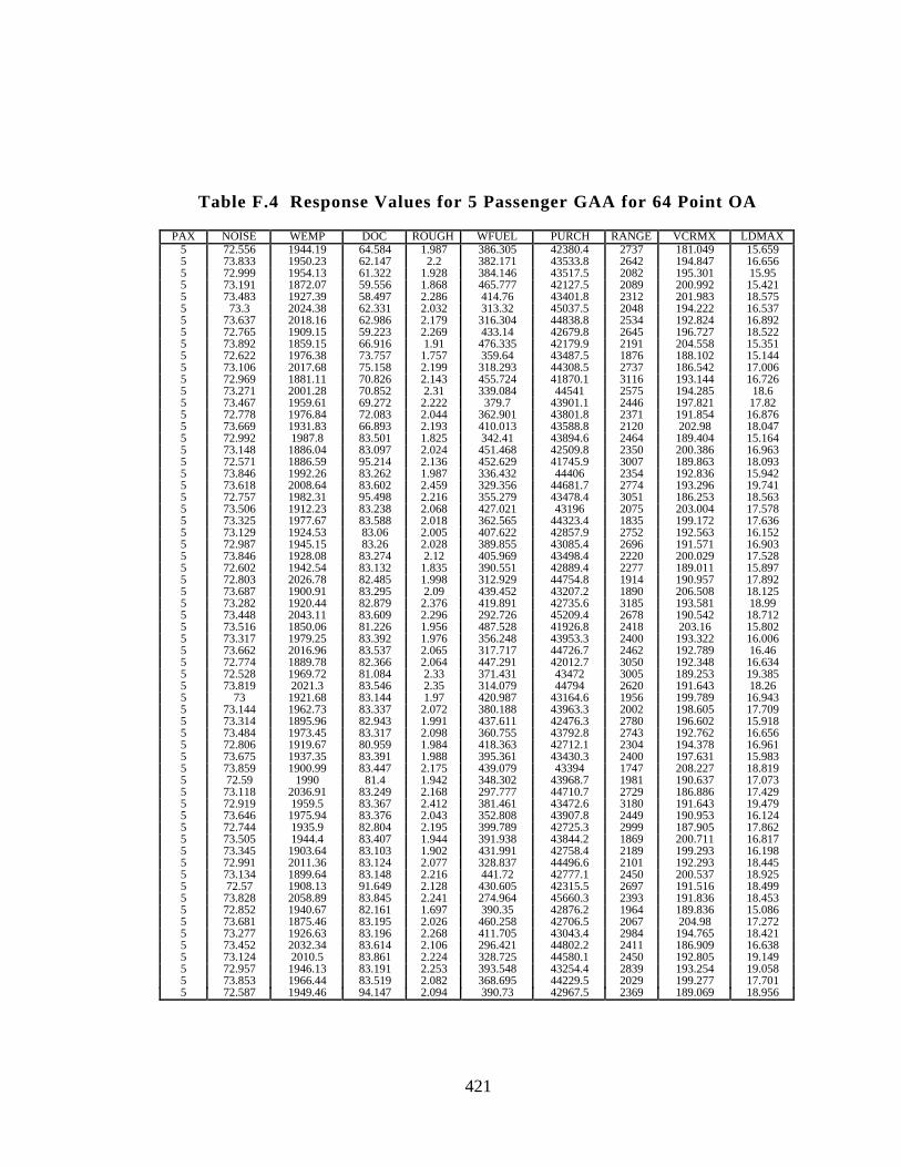
421
Table F.4 Response Values for 5 Passenger GAA for 64 Point OA
PAX NOISE WEMP DOC ROUGH WFUEL PURCH RANGE VCRMX LDMAX5 72.556 1944.19 64.584 1.987 386.305 42380.4 2737 181.049 15.6595 73.833 1950.23 62.147 2.2 382.171 43533.8 2642 194.847 16.6565 72.999 1954.13 61.322 1.928 384.146 43517.5 2082 195.301 15.955 73.191 1872.07 59.556 1.868 465.777 42127.5 2089 200.992 15.4215 73.483 1927.39 58.497 2.286 414.76 43401.8 2312 201.983 18.5755 73.3 2024.38 62.331 2.032 313.32 45037.5 2048 194.222 16.5375 73.637 2018.16 62.986 2.179 316.304 44838.8 2534 192.824 16.8925 72.765 1909.15 59.223 2.269 433.14 42679.8 2645 196.727 18.5225 73.892 1859.15 66.916 1.91 476.335 42179.9 2191 204.558 15.3515 72.622 1976.38 73.757 1.757 359.64 43487.5 1876 188.102 15.1445 73.106 2017.68 75.158 2.199 318.293 44308.5 2737 186.542 17.0065 72.969 1881.11 70.826 2.143 455.724 41870.1 3116 193.144 16.7265 73.271 2001.28 70.852 2.31 339.084 44541 2575 194.285 18.65 73.467 1959.61 69.272 2.222 379.7 43901.1 2446 197.821 17.825 72.778 1976.84 72.083 2.044 362.901 43801.8 2371 191.854 16.8765 73.669 1931.83 66.893 2.193 410.013 43588.8 2120 202.98 18.0475 72.992 1987.8 83.501 1.825 342.41 43894.6 2464 189.404 15.1645 73.148 1886.04 83.097 2.024 451.468 42509.8 2350 200.386 16.9635 72.571 1886.59 95.214 2.136 452.629 41745.9 3007 189.863 18.0935 73.846 1992.26 83.262 1.987 336.432 44406 2354 192.836 15.9425 73.618 2008.64 83.602 2.459 329.356 44681.7 2774 193.296 19.7415 72.757 1982.31 95.498 2.216 355.279 43478.4 3051 186.253 18.5635 73.506 1912.23 83.238 2.068 427.021 43196 2075 203.004 17.5785 73.325 1977.67 83.588 2.018 362.565 44323.4 1835 199.172 17.6365 73.129 1924.53 83.06 2.005 407.622 42857.9 2752 192.563 16.1525 72.987 1945.15 83.26 2.028 389.855 43085.4 2696 191.571 16.9035 73.846 1928.08 83.274 2.12 405.969 43498.4 2220 200.029 17.5285 72.602 1942.54 83.132 1.835 390.551 42889.4 2277 189.011 15.8975 72.803 2026.78 82.485 1.998 312.929 44754.8 1914 190.957 17.8925 73.687 1900.91 83.295 2.09 439.452 43207.2 1890 206.508 18.1255 73.282 1920.44 82.879 2.376 419.891 42735.6 3185 193.581 18.995 73.448 2043.11 83.609 2.296 292.726 45209.4 2678 190.542 18.7125 73.516 1850.06 81.226 1.956 487.528 41926.8 2418 203.16 15.8025 73.317 1979.25 83.392 1.976 356.248 43953.3 2400 193.322 16.0065 73.662 2016.96 83.537 2.065 317.717 44726.7 2462 192.789 16.465 72.774 1889.78 82.366 2.064 447.291 42012.7 3050 192.348 16.6345 72.528 1969.72 81.084 2.33 371.431 43472 3005 189.253 19.3855 73.819 2021.3 83.546 2.35 314.079 44794 2620 191.643 18.265 73 1921.68 83.144 1.97 420.987 43164.6 1956 199.789 16.9435 73.144 1962.73 83.337 2.072 380.188 43963.3 2002 198.605 17.7095 73.314 1895.96 82.943 1.991 437.611 42476.3 2780 196.602 15.9185 73.484 1973.45 83.317 2.098 360.755 43792.8 2743 192.762 16.6565 72.806 1919.67 80.959 1.984 418.363 42712.1 2304 194.378 16.9615 73.675 1937.35 83.391 1.988 395.361 43430.3 2400 197.631 15.9835 73.859 1900.99 83.447 2.175 439.079 43394 1747 208.227 18.8195 72.59 1990 81.4 1.942 348.302 43968.7 1981 190.637 17.0735 73.118 2036.91 83.249 2.168 297.777 44710.7 2729 186.886 17.4295 72.919 1959.5 83.367 2.412 381.461 43472.6 3180 191.643 19.4795 73.646 1975.94 83.376 2.043 352.808 43907.8 2449 190.953 16.1245 72.744 1935.9 82.804 2.195 399.789 42725.3 2999 187.905 17.8625 73.505 1944.4 83.407 1.944 391.938 43844.2 1869 200.711 16.8175 73.345 1903.64 83.103 1.902 431.991 42758.4 2189 199.293 16.1985 72.991 2011.36 83.124 2.077 328.837 44496.6 2101 192.293 18.4455 73.134 1899.64 83.148 2.216 441.72 42777.1 2450 200.537 18.9255 72.57 1908.13 91.649 2.128 430.605 42315.5 2697 191.516 18.4995 73.828 2058.89 83.845 2.241 274.964 45660.3 2393 191.836 18.4535 72.852 1940.67 82.161 1.697 390.35 42876.2 1964 189.836 15.0865 73.681 1875.46 83.195 2.026 460.258 42706.5 2067 204.98 17.2725 73.277 1926.63 83.196 2.268 411.705 43043.4 2984 194.765 18.4215 73.452 2032.34 83.614 2.106 296.421 44802.2 2411 186.909 16.6385 73.124 2010.5 83.861 2.224 328.725 44580.1 2450 192.805 19.1495 72.957 1946.13 83.191 2.253 393.548 43254.4 2839 193.254 19.0585 73.853 1966.44 83.519 2.082 368.695 44229.5 2029 199.277 17.7015 72.587 1949.46 94.147 2.094 390.73 42967.5 2369 189.069 18.956
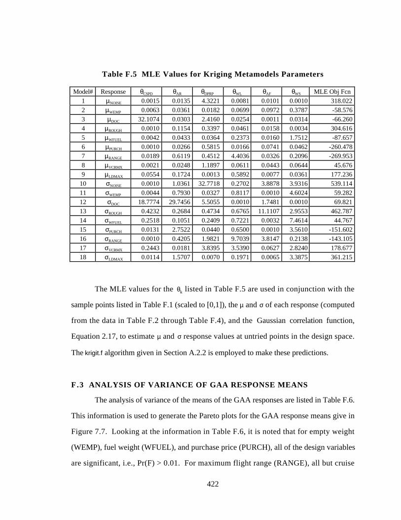
422
Table F.5 MLE Values for Kriging Metamodels Parameters
Model# Response θCSPD θAR θDPRP θWL θAF θWS MLE Obj Fcn
1 µNOISE 0.0015 0.0135 4.3221 0.0081 0.0101 0.0010 318.022
2 µWEMP 0.0063 0.0361 0.0182 0.0699 0.0972 0.3787 -58.576
3 µDOC 32.1074 0.0303 2.4160 0.0254 0.0011 0.0314 -66.260
4 µROUGH 0.0010 0.1154 0.3397 0.0461 0.0158 0.0034 304.616
5 µWFUEL 0.0042 0.0433 0.0364 0.2373 0.0160 1.7512 -87.657
6 µPURCH 0.0010 0.0266 0.5815 0.0166 0.0741 0.0462 -260.478
7 µRANGE 0.0189 0.6119 0.4512 4.4036 0.0326 0.2096 -269.953
8 µVCRMX 0.0021 0.0248 1.1897 0.0611 0.0443 0.0644 45.676
9 µLDMAX 0.0554 0.1724 0.0013 0.5892 0.0077 0.0361 177.236
10 σNOISE 0.0010 1.0361 32.7718 0.2702 3.8878 3.9316 539.114
11 σWEMP 0.0044 0.7930 0.0327 0.8117 0.0010 4.6024 59.282
12 σDOC 18.7774 29.7456 5.5055 0.0010 1.7481 0.0010 69.821
13 σROUGH 0.4232 0.2684 0.4734 0.6765 11.1107 2.9553 462.787
14 σWFUEL 0.2518 0.1051 0.2409 0.7221 0.0032 7.4614 44.767
15 σPURCH 0.0131 2.7522 0.0440 0.6500 0.0010 3.5610 -151.602
16 σRANGE 0.0010 0.4205 1.9821 9.7039 3.8147 0.2138 -143.105
17 σVCRMX 0.2443 0.0181 3.8395 3.5390 0.0627 2.8240 178.677
18 σLDMAX 0.0114 1.5707 0.0070 0.1971 0.0065 3.3875 361.215
The MLE values for the θk listed in Table F.5 are used in conjunction with the
sample points listed in Table F.1 (scaled to [0,1]), the µ and σ of each response (computed
from the data in Table F.2 through Table F.4), and the Gaussian correlation function,
Equation 2.17, to estimate µ and σ response values at untried points in the design space.
The krigit.f algorithm given in Section A.2.2 is employed to make these predictions.
F.3 ANALYSIS OF VARIANCE OF GAA RESPONSE MEANS
The analysis of variance of the means of the GAA responses are listed in Table F.6.
This information is used to generate the Pareto plots for the GAA response means give in
Figure 7.7. Looking at the information in Table F.6, it is noted that for empty weight
(WEMP), fuel weight (WFUEL), and purchase price (PURCH), all of the design variables
are significant, i.e., Pr(F) > 0.01. For maximum flight range (RANGE), all but cruise
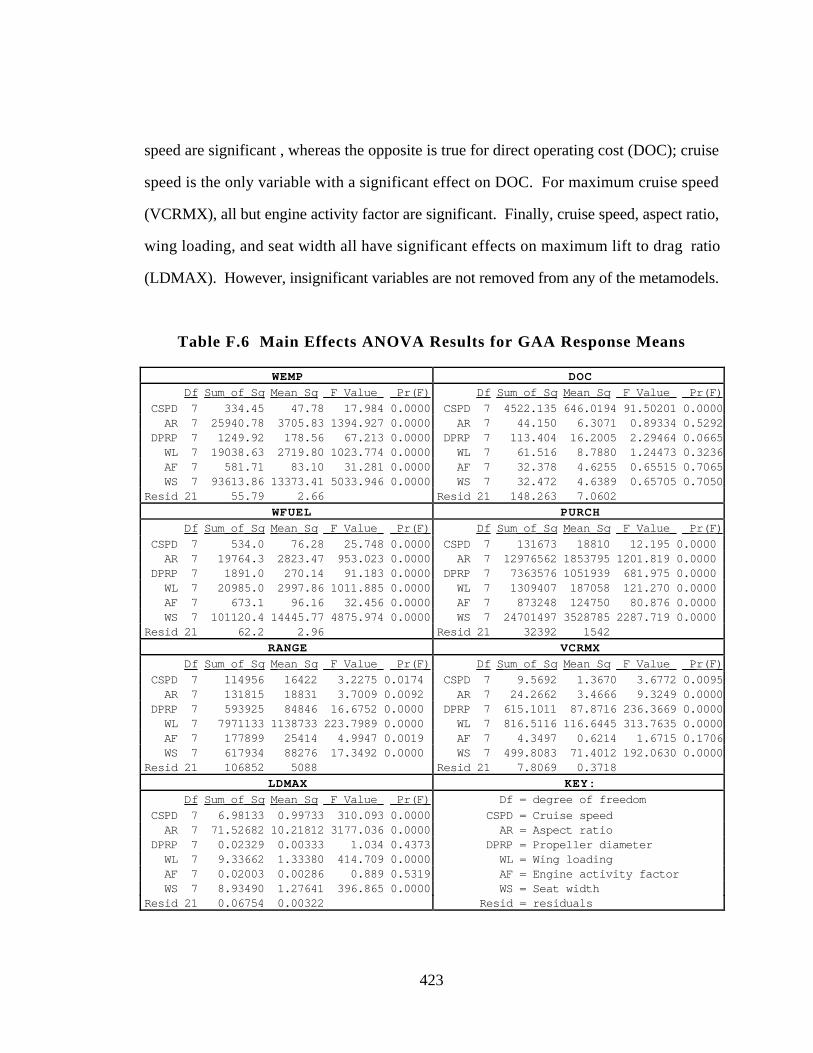
423
speed are significant , whereas the opposite is true for direct operating cost (DOC); cruise
speed is the only variable with a significant effect on DOC. For maximum cruise speed
(VCRMX), all but engine activity factor are significant. Finally, cruise speed, aspect ratio,
wing loading, and seat width all have significant effects on maximum lift to drag ratio
(LDMAX). However, insignificant variables are not removed from any of the metamodels.
Table F.6 Main Effects ANOVA Results for GAA Response Means
WEMP DOC
Df Sum of Sq Mean Sq F Value Pr(F) Df Sum of Sq Mean Sq F Value Pr(F)
CSPD 7 334.45 47.78 17.984 0.0000 CSPD 7 4522.135 646.0194 91.50201 0.0000 AR 7 25940.78 3705.83 1394.927 0.0000 AR 7 44.150 6.3071 0.89334 0.5292 DPRP 7 1249.92 178.56 67.213 0.0000 DPRP 7 113.404 16.2005 2.29464 0.0665 WL 7 19038.63 2719.80 1023.774 0.0000 WL 7 61.516 8.7880 1.24473 0.3236 AF 7 581.71 83.10 31.281 0.0000 AF 7 32.378 4.6255 0.65515 0.7065 WS 7 93613.86 13373.41 5033.946 0.0000 WS 7 32.472 4.6389 0.65705 0.7050Resid 21 55.79 2.66 Resid 21 148.263 7.0602
WFUEL PURCH
Df Sum of Sq Mean Sq F Value Pr(F) Df Sum of Sq Mean Sq F Value Pr(F)
CSPD 7 534.0 76.28 25.748 0.0000 CSPD 7 131673 18810 12.195 0.0000 AR 7 19764.3 2823.47 953.023 0.0000 AR 7 12976562 1853795 1201.819 0.0000 DPRP 7 1891.0 270.14 91.183 0.0000 DPRP 7 7363576 1051939 681.975 0.0000 WL 7 20985.0 2997.86 1011.885 0.0000 WL 7 1309407 187058 121.270 0.0000 AF 7 673.1 96.16 32.456 0.0000 AF 7 873248 124750 80.876 0.0000 WS 7 101120.4 14445.77 4875.974 0.0000 WS 7 24701497 3528785 2287.719 0.0000Resid 21 62.2 2.96 Resid 21 32392 1542
RANGE VCRMX
Df Sum of Sq Mean Sq F Value Pr(F) Df Sum of Sq Mean Sq F Value Pr(F)
CSPD 7 114956 16422 3.2275 0.0174 CSPD 7 9.5692 1.3670 3.6772 0.0095 AR 7 131815 18831 3.7009 0.0092 AR 7 24.2662 3.4666 9.3249 0.0000 DPRP 7 593925 84846 16.6752 0.0000 DPRP 7 615.1011 87.8716 236.3669 0.0000 WL 7 7971133 1138733 223.7989 0.0000 WL 7 816.5116 116.6445 313.7635 0.0000 AF 7 177899 25414 4.9947 0.0019 AF 7 4.3497 0.6214 1.6715 0.1706 WS 7 617934 88276 17.3492 0.0000 WS 7 499.8083 71.4012 192.0630 0.0000Resid 21 106852 5088 Resid 21 7.8069 0.3718
LDMAX KEY:
Df Sum of Sq Mean Sq F Value Pr(F) Df = degree of freedom
CSPD 7 6.98133 0.99733 310.093 0.0000 CSPD = Cruise speed AR 7 71.52682 10.21812 3177.036 0.0000 AR = Aspect ratio DPRP 7 0.02329 0.00333 1.034 0.4373 DPRP = Propeller diameter WL 7 9.33662 1.33380 414.709 0.0000 WL = Wing loading AF 7 0.02003 0.00286 0.889 0.5319 AF = Engine activity factor WS 7 8.93490 1.27641 396.865 0.0000 WS = Seat widthResid 21 0.06754 0.00322 Resid = residuals
424
F.4 ADDITIONAL DESIGN SCENARIOS FOR STUDY GAA PRODUCTPLATFORM USING Cdk FORMULATION
In all, eight different design scenarios are considered to investigate several
performance and economic tradeoffs within the product family, see Table F.7. Only the
first three scenarios are discussed in Section 7.5 in regards to the PPCEM product
platform. These remaining scenarios are described as follows.
Group I - Tradeoff studies: includes Scenarios 1, 2 and 3. In these scenarios, the
tradeoffs of achieving a set of conflicting goals are examined. An overall tradeoff
study with all goals weighted equally is performed in Scenario 1. Scenario 2 is an
economic tradeoff study with WEMP, PURCH, and DOC given first priority. A
performance tradeoff study with WFUEL, VCRMX, RANGE, and LDMAX
ranked highest is Scenario 3. The deviation function formulations for Scenarios 1-
3 are summarized in Table F.7. In the table, PLEV# represents the priority level.
Group II - Economic tradeoff scenarios: includes Scenarios 4 and 5. In these
two scenarios, the economic goals are given first priority over performance
concerns. Two scenarios are considered, one with manufacturing considerations
(WEMP and PURCH) as the main driver, Scenario 4, and one with direct operating
cost (DOC) as the main driver, Scenario 5. See Table F.7 for the corresponding
deviation function formulations.
Group III - Performance tradeoff scenarios: includes Scenario 6, 7, and 8. In
these scenarios performance considerations are given first priority; economics ranks
second. Scenario 6 is based on speed considerations with VCRMX and WFUEL
ranked first, Scenario 7 is based on aerodynamic considerations with LDMAX
ranked first, and Scenario 8 is based on the flight distance with RANGE ranked
first. The corresponding deviation function formulations are listed in Table F.7.
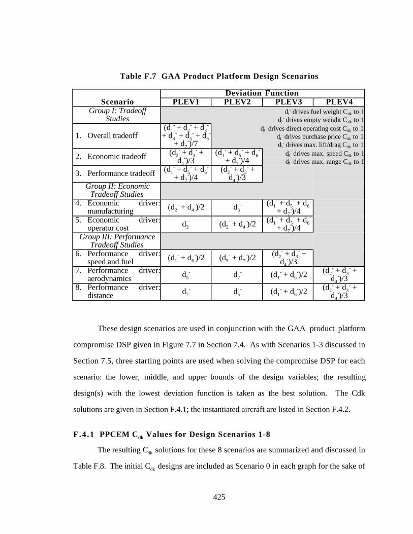
425
Table F.7 GAA Product Platform Design Scenarios
Deviation FunctionScenario PLEV1 PLEV2 PLEV3 PLEV4
Group I: TradeoffStudies
d1- drives fuel weight Cdk to 1
d2- drives empty weight Cdk to 1
1. Overall tradeoff(d1
- + d2- + d3
-
+ d4- + d5
- + d6-
+ d7-)/7
d3- drives direct operating cost Cdk to 1
d4- drives purchase price Cdk to 1
d5- drives max. lift/drag Cdk to 1
2. Economic tradeoff (d2- + d3
- +d4
-)/3(d1
- + d5- + d6
-
+ d7-)/4
d6- drives max. speed Cdk to 1
d7- drives max. range Cdk to 1
3. Performance tradeoff (d1- + d5
- + d6-
+ d7-)/4
(d2- + d3
- +d4
-)/3Group II: Economic
Tradeoff Studies4. Economic driver:
manufacturing (d2- + d4
-)/2 d3- (d1
- + d5- + d6
-
+ d7-)/4
5. Economic driver:operator cost d3
- (d2- + d4
-)/2 (d1- + d5
- + d6-
+ d7-)/4
Group III: PerformanceTradeoff Studies
6. Performance driver:speed and fuel (d1
- + d6-)/2 (d5
- + d7-)/2 (d2
- + d3- +
d4-)/3
7. Performance driver:aerodynamics d5
- d7- (d1
- + d6-)/2 (d2
- + d3- +
d4-)/3
8. Performance driver:distance d7
- d5- (d1
- + d6-)/2 (d2
- + d3- +
d4-)/3
These design scenarios are used in conjunction with the GAA product platform
compromise DSP given in Figure 7.7 in Section 7.4. As with Scenarios 1-3 discussed in
Section 7.5, three starting points are used when solving the compromise DSP for each
scenario: the lower, middle, and upper bounds of the design variables; the resulting
design(s) with the lowest deviation function is taken as the best solution. The Cdk
solutions are given in Section F.4.1; the instantiated aircraft are listed in Section F.4.2.
F.4 .1 PPCEM Cdk Values for Design Scenarios 1-8
The resulting Cdk solutions for these 8 scenarios are summarized and discussed in
Table F.8. The initial Cdk designs are included as Scenario 0 in each graph for the sake of
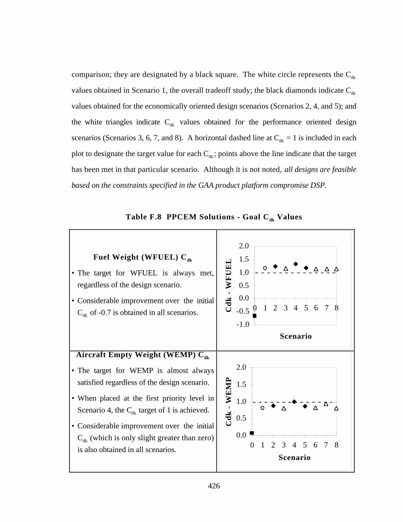
426
comparison; they are designated by a black square. The white circle represents the Cdk
values obtained in Scenario 1, the overall tradeoff study; the black diamonds indicate Cdk
values obtained for the economically oriented design scenarios (Scenarios 2, 4, and 5); and
the white triangles indicate Cdk values obtained for the performance oriented design
scenarios (Scenarios 3, 6, 7, and 8). A horizontal dashed line at Cdk = 1 is included in each
plot to designate the target value for each Cdk; points above the line indicate that the target
has been met in that particular scenario. Although it is not noted, all designs are feasible
based on the constraints specified in the GAA product platform compromise DSP.
Table F.8 PPCEM Solutions - Goal Cdk Values
Fuel Weight (WFUEL) Cdk
• The target for WFUEL is always met,
regardless of the design scenario.
• Considerable improvement over the initial
Cdk of -0.7 is obtained in all scenarios.
-1.0
-0.5
0.0
0.5
1.0
1.5
2.0
0 1 2 3 4 5 6 7 8
Scenario
Cd
k -
WF
UE
L
Aircraft Empty Weight (WEMP) Cdk
• The target for WEMP is almost always
satisfied regardless of the design scenario.
• When placed at the first priority level in
Scenario 4, the Cdk target of 1 is achieved.
• Considerable improvement over the initial
Cdk (which is only slight greater than zero)
is also obtained in all scenarios.
0.0
0.5
1.0
1.5
2.0
0 1 2 3 4 5 6 7 8
Scenario
Cd
k -
WE
MP
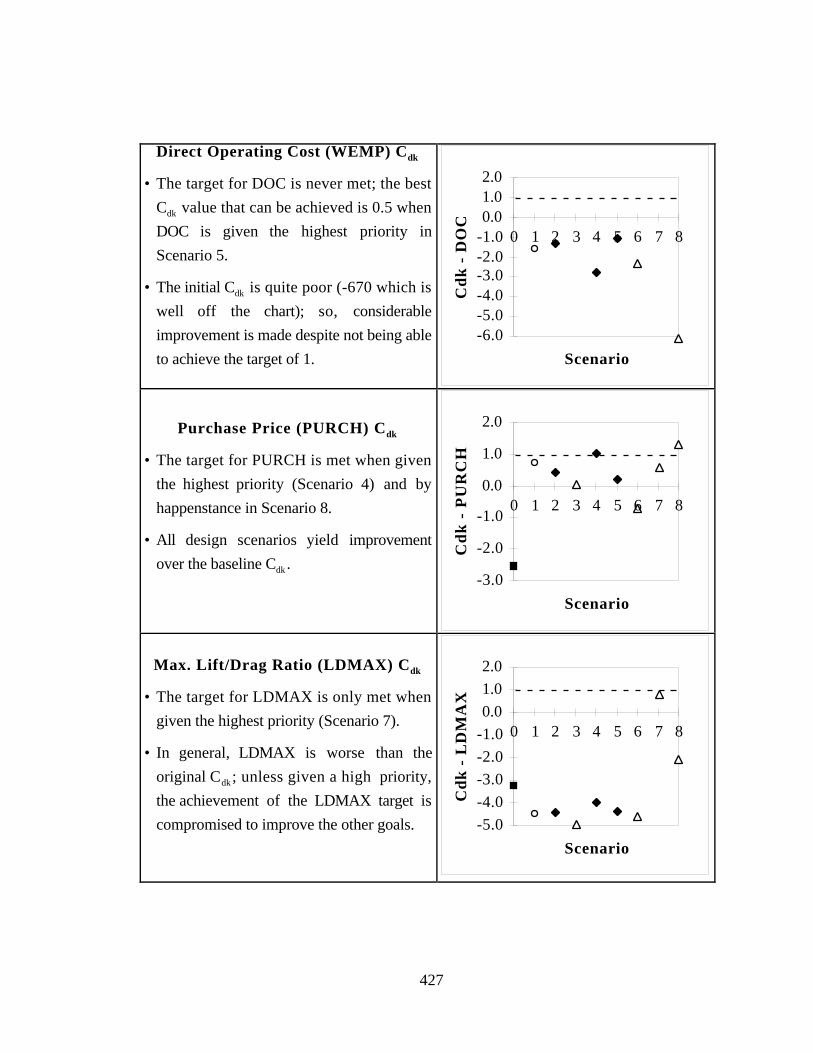
427
Direct Operating Cost (WEMP) Cdk
• The target for DOC is never met; the best
Cdk value that can be achieved is 0.5 when
DOC is given the highest priority in
Scenario 5.
• The initial Cdk is quite poor (-670 which is
well off the chart); so, considerable
improvement is made despite not being able
to achieve the target of 1.
-6.0-5.0-4.0-3.0-2.0-1.00.01.02.0
0 1 2 3 4 5 6 7 8
Scenario
Cd
k -
DO
C
Purchase Price (PURCH) Cdk
• The target for PURCH is met when given
the highest priority (Scenario 4) and by
happenstance in Scenario 8.
• All design scenarios yield improvement
over the baseline Cdk . -3.0
-2.0
-1.0
0.0
1.0
2.0
0 1 2 3 4 5 6 7 8
Scenario
Cd
k -
PU
RC
H
Max. Lift/Drag Ratio (LDMAX) Cdk
• The target for LDMAX is only met when
given the highest priority (Scenario 7).
• In general, LDMAX is worse than the
original Cdk; unless given a high priority,
the achievement of the LDMAX target is
compromised to improve the other goals. -5.0
-4.0
-3.0
-2.0
-1.0
0.0
1.0
2.0
0 1 2 3 4 5 6 7 8
Scenario
Cd
k -
LD
MA
X
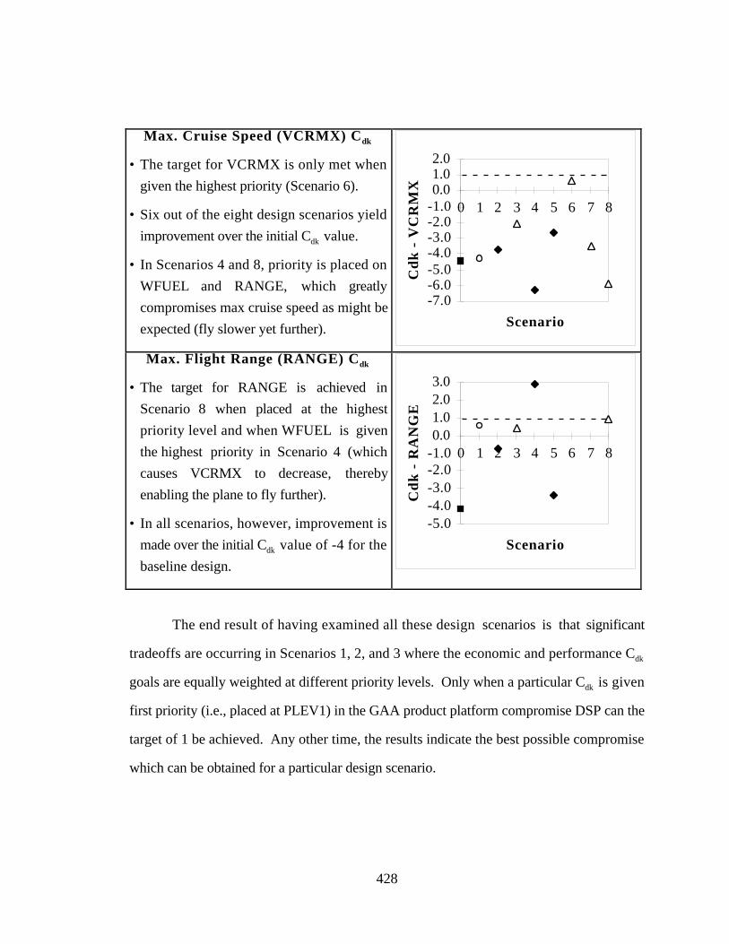
428
Max. Cruise Speed (VCRMX) Cdk
• The target for VCRMX is only met when
given the highest priority (Scenario 6).
• Six out of the eight design scenarios yield
improvement over the initial Cdk value.
• In Scenarios 4 and 8, priority is placed on
WFUEL and RANGE, which greatly
compromises max cruise speed as might be
expected (fly slower yet further).
-7.0-6.0-5.0-4.0-3.0-2.0-1.00.01.02.0
0 1 2 3 4 5 6 7 8
Scenario
Cd
k -
VC
RM
X
Max. Flight Range (RANGE) Cdk
• The target for RANGE is achieved in
Scenario 8 when placed at the highest
priority level and when WFUEL is given
the highest priority in Scenario 4 (which
causes VCRMX to decrease, thereby
enabling the plane to fly further).
• In all scenarios, however, improvement is
made over the initial Cdk value of -4 for the
baseline design.
-5.0-4.0-3.0-2.0-1.00.01.02.03.0
0 1 2 3 4 5 6 7 8
Scenario
Cd
k -
RA
NG
E
The end result of having examined all these design scenarios is that significant
tradeoffs are occurring in Scenarios 1, 2, and 3 where the economic and performance Cdk
goals are equally weighted at different priority levels. Only when a particular Cdk is given
first priority (i.e., placed at PLEV1) in the GAA product platform compromise DSP can the
target of 1 be achieved. Any other time, the results indicate the best possible compromise
which can be obtained for a particular design scenario.
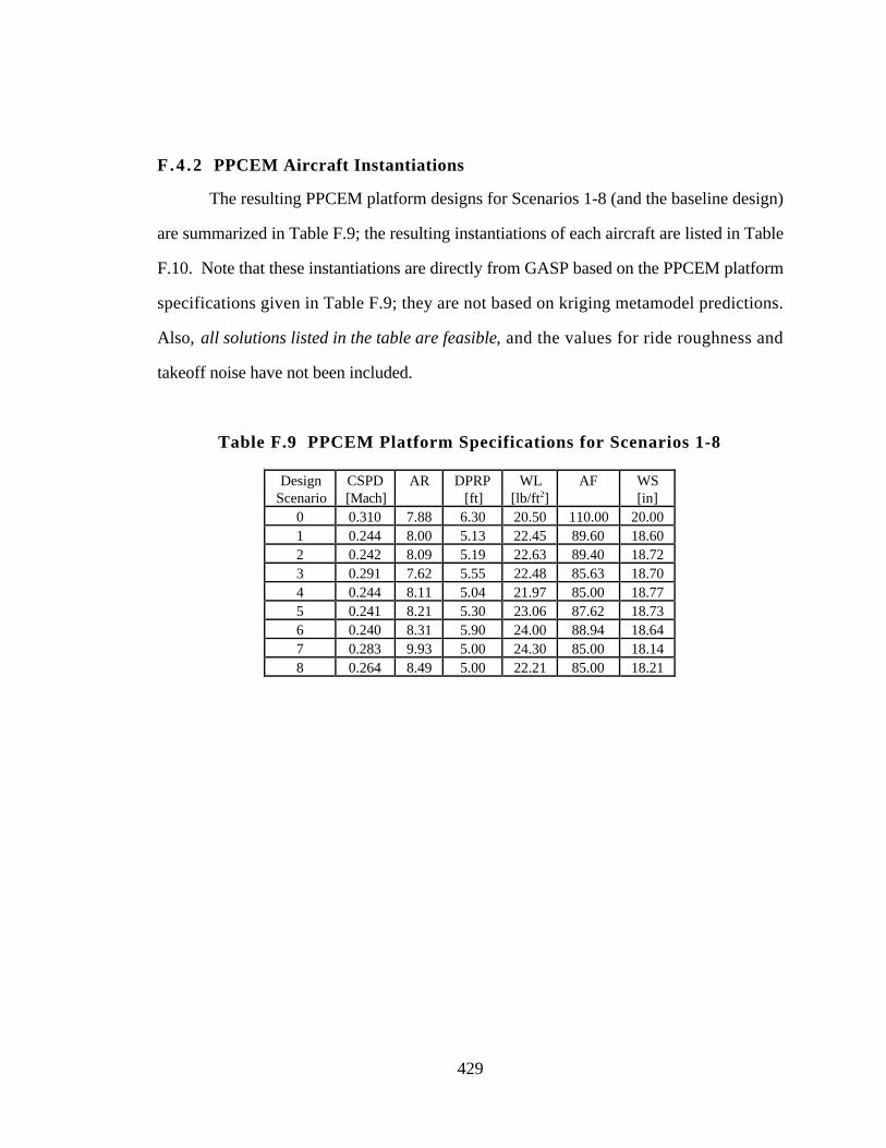
429
F.4 .2 PPCEM Aircraft Instantiations
The resulting PPCEM platform designs for Scenarios 1-8 (and the baseline design)
are summarized in Table F.9; the resulting instantiations of each aircraft are listed in Table
F.10. Note that these instantiations are directly from GASP based on the PPCEM platform
specifications given in Table F.9; they are not based on kriging metamodel predictions.
Also, all solutions listed in the table are feasible, and the values for ride roughness and
takeoff noise have not been included.
Table F.9 PPCEM Platform Specifications for Scenarios 1-8
Design CSPD AR DPRP WL AF WSScenario [Mach] [ft] [lb/ft2] [in]
0 0.310 7.88 6.30 20.50 110.00 20.001 0.244 8.00 5.13 22.45 89.60 18.602 0.242 8.09 5.19 22.63 89.40 18.723 0.291 7.62 5.55 22.48 85.63 18.704 0.244 8.11 5.04 21.97 85.00 18.775 0.241 8.21 5.30 23.06 87.62 18.736 0.240 8.31 5.90 24.00 88.94 18.647 0.283 9.93 5.00 24.30 85.00 18.148 0.264 8.49 5.00 22.21 85.00 18.21
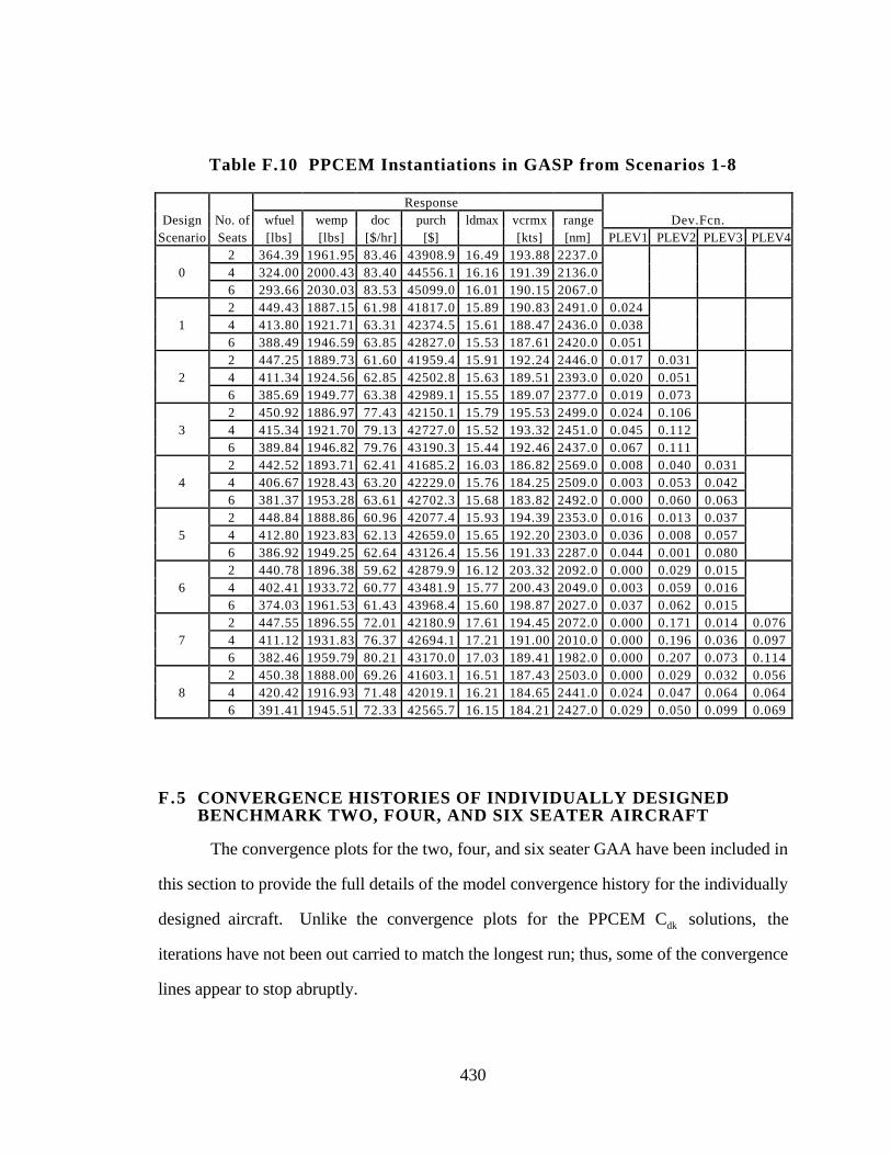
430
Table F.10 PPCEM Instantiations in GASP from Scenarios 1-8
ResponseDesign No. of wfuel wemp doc purch ldmax vcrmx range Dev.Fcn.
Scenario Seats [lbs] [lbs] [$/hr] [$] [kts] [nm] PLEV1 PLEV2 PLEV3 PLEV42 364.39 1961.95 83.46 43908.9 16.49 193.88 2237.0
0 4 324.00 2000.43 83.40 44556.1 16.16 191.39 2136.06 293.66 2030.03 83.53 45099.0 16.01 190.15 2067.02 449.43 1887.15 61.98 41817.0 15.89 190.83 2491.0 0.024
1 4 413.80 1921.71 63.31 42374.5 15.61 188.47 2436.0 0.0386 388.49 1946.59 63.85 42827.0 15.53 187.61 2420.0 0.0512 447.25 1889.73 61.60 41959.4 15.91 192.24 2446.0 0.017 0.031
2 4 411.34 1924.56 62.85 42502.8 15.63 189.51 2393.0 0.020 0.0516 385.69 1949.77 63.38 42989.1 15.55 189.07 2377.0 0.019 0.0732 450.92 1886.97 77.43 42150.1 15.79 195.53 2499.0 0.024 0.106
3 4 415.34 1921.70 79.13 42727.0 15.52 193.32 2451.0 0.045 0.1126 389.84 1946.82 79.76 43190.3 15.44 192.46 2437.0 0.067 0.1112 442.52 1893.71 62.41 41685.2 16.03 186.82 2569.0 0.008 0.040 0.031
4 4 406.67 1928.43 63.20 42229.0 15.76 184.25 2509.0 0.003 0.053 0.0426 381.37 1953.28 63.61 42702.3 15.68 183.82 2492.0 0.000 0.060 0.0632 448.84 1888.86 60.96 42077.4 15.93 194.39 2353.0 0.016 0.013 0.037
5 4 412.80 1923.83 62.13 42659.0 15.65 192.20 2303.0 0.036 0.008 0.0576 386.92 1949.25 62.64 43126.4 15.56 191.33 2287.0 0.044 0.001 0.0802 440.78 1896.38 59.62 42879.9 16.12 203.32 2092.0 0.000 0.029 0.015
6 4 402.41 1933.72 60.77 43481.9 15.77 200.43 2049.0 0.003 0.059 0.0166 374.03 1961.53 61.43 43968.4 15.60 198.87 2027.0 0.037 0.062 0.0152 447.55 1896.55 72.01 42180.9 17.61 194.45 2072.0 0.000 0.171 0.014 0.076
7 4 411.12 1931.83 76.37 42694.1 17.21 191.00 2010.0 0.000 0.196 0.036 0.0976 382.46 1959.79 80.21 43170.0 17.03 189.41 1982.0 0.000 0.207 0.073 0.1142 450.38 1888.00 69.26 41603.1 16.51 187.43 2503.0 0.000 0.029 0.032 0.056
8 4 420.42 1916.93 71.48 42019.1 16.21 184.65 2441.0 0.024 0.047 0.064 0.0646 391.41 1945.51 72.33 42565.7 16.15 184.21 2427.0 0.029 0.050 0.099 0.069
F.5 CONVERGENCE HISTORIES OF INDIVIDUALLY DESIGNEDBENCHMARK TWO, FOUR, AND SIX SEATER AIRCRAFT
The convergence plots for the two, four, and six seater GAA have been included in
this section to provide the full details of the model convergence history for the individually
designed aircraft. Unlike the convergence plots for the PPCEM Cdk solutions, the
iterations have not been out carried to match the longest run; thus, some of the convergence
lines appear to stop abruptly.
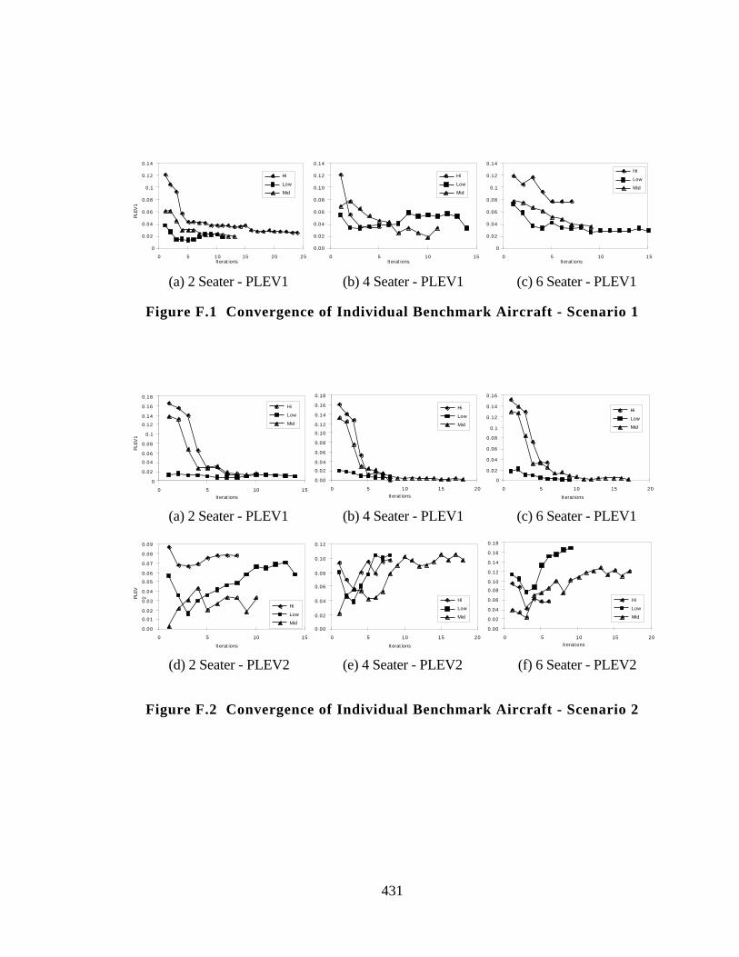
431
0
0.02
0.04
0.06
0.08
0.1
0.12
0.14
0 5 10 15 20 25Iterations
PLEV
1
Hi
Low
Mid
0.00
0.02
0.04
0.06
0.08
0.10
0.12
0.14
0 5 10 15Iterations
Hi
Low
Mid
0
0.02
0.04
0.06
0.08
0.1
0.12
0.14
0 5 10 15Iterations
Hi
Low
Mid
(a) 2 Seater - PLEV1 (b) 4 Seater - PLEV1 (c) 6 Seater - PLEV1
Figure F.1 Convergence of Individual Benchmark Aircraft - Scenario 1
0
0.02
0.04
0.06
0.08
0.1
0.12
0.14
0.16
0.18
0 5 10 15Iterations
PLEV
1
Hi
Low
Mid
0.00
0.02
0.04
0.06
0.08
0.10
0.12
0.14
0.16
0.18
0 5 10 15 20Iterations
Hi
Low
Mid
0
0.02
0.04
0.06
0.08
0.1
0.12
0.14
0.16
0 5 10 15 20
Iterations
Hi
Low
Mid
(a) 2 Seater - PLEV1 (b) 4 Seater - PLEV1 (c) 6 Seater - PLEV1
0.00
0.01
0.02
0.03
0.04
0.05
0.06
0.07
0.08
0.09
0 5 10 15
Iterations
PLEV
2
Hi
Low
Mid0.00
0.02
0.04
0.06
0.08
0.10
0.12
0 5 10 15 20
Iterations
Hi
Low
Mid
0.00
0.02
0.04
0.06
0.08
0.10
0.12
0.14
0.16
0.18
0 5 10 15 20Iterations
Hi
Low
Mid
(d) 2 Seater - PLEV2 (e) 4 Seater - PLEV2 (f) 6 Seater - PLEV2
Figure F.2 Convergence of Individual Benchmark Aircraft - Scenario 2
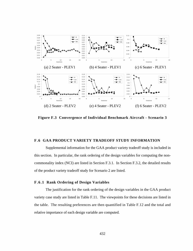
432
0.00
0.01
0.02
0.03
0.04
0.05
0.06
0.07
0.08
0.09
0 5 10 15 20Iterations
PLEV
1Hi
Low
Mid
0.00
0.01
0.02
0.03
0.04
0.05
0.06
0.07
0.08
0.09
0.10
0 5 10 15Iterations
Hi
Low
Mid
0
0.02
0.04
0.06
0.08
0.1
0.12
0 5 10 15Iterations
Hi
Low
Mid
(a) 2 Seater - PLEV1 (b) 4 Seater - PLEV1 (c) 6 Seater - PLEV1
0
0.02
0.04
0.06
0.08
0.1
0.12
0.14
0.16
0.18
0 5 10 15 20Iterations
PLEV
2
Hi
Low
Mid
0.00
0.02
0.04
0.06
0.08
0.10
0.12
0.14
0.16
0.18
0 5 10 15Iterations
Hi
Low
Mid
0
0.02
0.04
0.06
0.08
0.1
0.12
0.14
0.16
0 5 10 15Iterations
Hi
Low
Mid
(d) 2 Seater - PLEV2 (e) 4 Seater - PLEV2 (f) 6 Seater - PLEV2
Figure F.3 Convergence of Individual Benchmark Aircraft - Scenario 3
F.6 GAA PRODUCT VARIETY TRADEOFF STUDY INFORMATION
Supplemental information for the GAA product variety tradeoff study is included in
this section. In particular, the rank ordering of the design variables for computing the non-
commonality index (NCI) are listed in Section F.3.1. In Section F.3.2, the detailed results
of the product variety tradeoff study for Scenario 2 are listed.
F.6 .1 Rank Ordering of Design Variables
The justification for the rank ordering of the design variables in the GAA product
variety case study are listed in Table F.11. The viewpoints for these decisions are listed in
the table. The resulting preferences are then quantified in Table F.12 and the total and
relative importance of each design variable are computed.
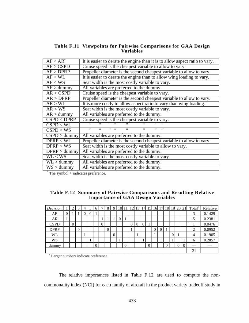
433
Table F.11 Viewpoints for Pairwise Comparisons for GAA DesignVariables
AF < AR* It is easier to derate the engine than it is to allow aspect ratio to vary.AF > CSPD Cruise speed is the cheapest variable to allow to vary.AF > DPRP Propeller diameter is the second cheapest variable to allow to vary.AF < WL It is easier to derate the engine than to allow wing loading to vary.AF < WS Seat width is the most costly variable to vary.AF > dummy All variables are preferred to the dummy.AR > CSPD Cruise speed is the cheapest variable to vary.AR > DPRP Propeller diameter is the second cheapest variable to allow to vary.AR > WL It is more costly to allow aspect ratio to vary than wing loading.AR < WS Seat width is the most costly variable to vary.AR > dummy All variables are preferred to the dummy.CSPD < DPRP Cruise speed is the cheapest variable to vary.CSPD < WL “ “ “ “ “ “ “ “CSPD < WS “ “ “ “ “ “ “ “CSPD > dummy All variables are preferred to the dummy.DPRP < WL Propeller diameter is the second cheapest variable to allow to vary.DPRP < WS Seat width is the most costly variable to allow to vary.DPRP > dummy All variables are preferred to the dummy.WL < WS Seat width is the most costly variable to vary.WL > dummy All variables are preferred to the dummy.WS > dummy All variables are preferred to the dummy.
* The symbol > indicates preference.
Table F.12 Summary of Pairwise Comparisons and Resulting RelativeImportance of GAA Design Variables
Decision: 1 2 3 4 5 6 7 8 9 10 11 12 13 14 15 16 17 18 19 20 21 Total† RelativeAF 0 1 1 0 0 1 3 0.1429AR 1 1 1 1 0 1 5 0.2381
CSPD 0 0 0 0 0 1 1 0.0476DPRP 0 0 1 0 0 1 2 0.0952WL 1 0 1 1 0 1 4 0.1905WS 1 1 1 1 1 1 6 0.2857
dummy 0 0 0 0 0 0 — —21
† Larger numbers indicate preference.
The relative importances listed in Table F.12 are used to compute the non-
commonality index (NCI) for each family of aircraft in the product variety tradeoff study in
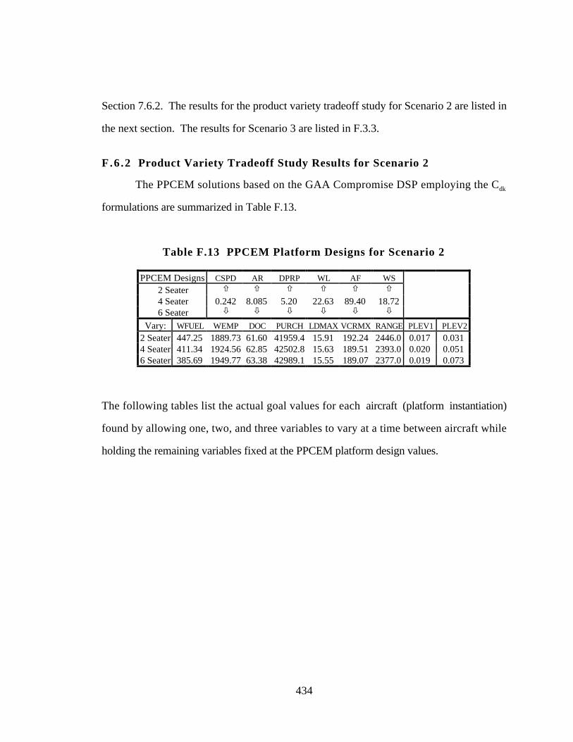
434
Section 7.6.2. The results for the product variety tradeoff study for Scenario 2 are listed in
the next section. The results for Scenario 3 are listed in F.3.3.
F.6 .2 Product Variety Tradeoff Study Results for Scenario 2
The PPCEM solutions based on the GAA Compromise DSP employing the Cdk
formulations are summarized in Table F.13.
Table F.13 PPCEM Platform Designs for Scenario 2
PPCEM Designs CSPD AR DPRP WL AF WS
2 Seater ñ ñ ñ ñ ñ ñ
4 Seater 0.242 8.085 5.20 22.63 89.40 18.726 Seater ò ò ò ò ò ò
Vary: WFUEL WEMP DOC PURCH LDMAX VCRMX RANGE PLEV1 PLEV2
2 Seater 447.25 1889.73 61.60 41959.4 15.91 192.24 2446.0 0.017 0.0314 Seater 411.34 1924.56 62.85 42502.8 15.63 189.51 2393.0 0.020 0.0516 Seater 385.69 1949.77 63.38 42989.1 15.55 189.07 2377.0 0.019 0.073
The following tables list the actual goal values for each aircraft (platform instantiation)
found by allowing one, two, and three variables to vary at a time between aircraft while
holding the remaining variables fixed at the PPCEM platform design values.
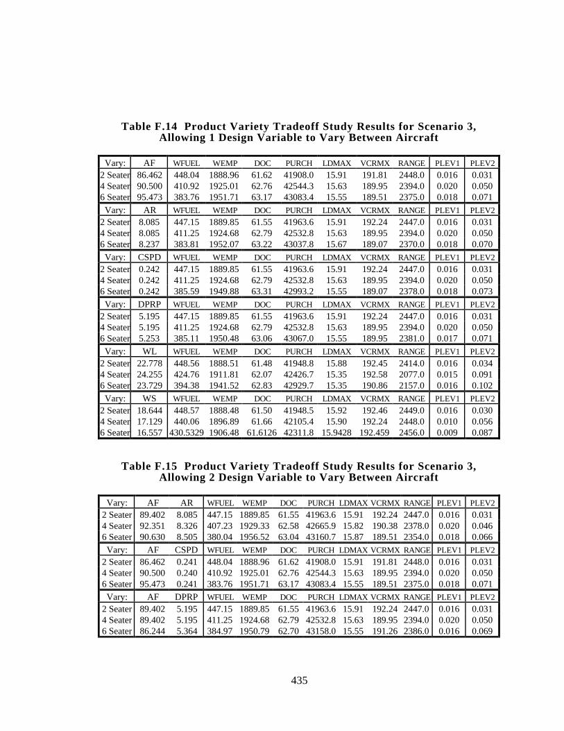
435
Table F.14 Product Variety Tradeoff Study Results for Scenario 3,Allowing 1 Design Variable to Vary Between Aircraft
Vary: AF WFUEL WEMP DOC PURCH LDMAX VCRMX RANGE PLEV1 PLEV2
2 Seater 86.462 448.04 1888.96 61.62 41908.0 15.91 191.81 2448.0 0.016 0.0314 Seater 90.500 410.92 1925.01 62.76 42544.3 15.63 189.95 2394.0 0.020 0.0506 Seater 95.473 383.76 1951.71 63.17 43083.4 15.55 189.51 2375.0 0.018 0.071
Vary: AR WFUEL WEMP DOC PURCH LDMAX VCRMX RANGE PLEV1 PLEV2
2 Seater 8.085 447.15 1889.85 61.55 41963.6 15.91 192.24 2447.0 0.016 0.0314 Seater 8.085 411.25 1924.68 62.79 42532.8 15.63 189.95 2394.0 0.020 0.0506 Seater 8.237 383.81 1952.07 63.22 43037.8 15.67 189.07 2370.0 0.018 0.070
Vary: CSPD WFUEL WEMP DOC PURCH LDMAX VCRMX RANGE PLEV1 PLEV2
2 Seater 0.242 447.15 1889.85 61.55 41963.6 15.91 192.24 2447.0 0.016 0.0314 Seater 0.242 411.25 1924.68 62.79 42532.8 15.63 189.95 2394.0 0.020 0.0506 Seater 0.242 385.59 1949.88 63.31 42993.2 15.55 189.07 2378.0 0.018 0.073
Vary: DPRP WFUEL WEMP DOC PURCH LDMAX VCRMX RANGE PLEV1 PLEV2
2 Seater 5.195 447.15 1889.85 61.55 41963.6 15.91 192.24 2447.0 0.016 0.0314 Seater 5.195 411.25 1924.68 62.79 42532.8 15.63 189.95 2394.0 0.020 0.0506 Seater 5.253 385.11 1950.48 63.06 43067.0 15.55 189.95 2381.0 0.017 0.071
Vary: WL WFUEL WEMP DOC PURCH LDMAX VCRMX RANGE PLEV1 PLEV2
2 Seater 22.778 448.56 1888.51 61.48 41948.8 15.88 192.45 2414.0 0.016 0.0344 Seater 24.255 424.76 1911.81 62.07 42426.7 15.35 192.58 2077.0 0.015 0.0916 Seater 23.729 394.38 1941.52 62.83 42929.7 15.35 190.86 2157.0 0.016 0.102
Vary: WS WFUEL WEMP DOC PURCH LDMAX VCRMX RANGE PLEV1 PLEV2
2 Seater 18.644 448.57 1888.48 61.50 41948.5 15.92 192.46 2449.0 0.016 0.0304 Seater 17.129 440.06 1896.89 61.66 42105.4 15.90 192.24 2448.0 0.010 0.0566 Seater 16.557 430.5329 1906.48 61.6126 42311.8 15.9428 192.459 2456.0 0.009 0.087
Table F.15 Product Variety Tradeoff Study Results for Scenario 3,Allowing 2 Design Variable to Vary Between Aircraft
Vary: AF AR WFUEL WEMP DOC PURCH LDMAX VCRMX RANGE PLEV1 PLEV2
2 Seater 89.402 8.085 447.15 1889.85 61.55 41963.6 15.91 192.24 2447.0 0.016 0.0314 Seater 92.351 8.326 407.23 1929.33 62.58 42665.9 15.82 190.38 2378.0 0.020 0.0466 Seater 90.630 8.505 380.04 1956.52 63.04 43160.7 15.87 189.51 2354.0 0.018 0.066
Vary: AF CSPD WFUEL WEMP DOC PURCH LDMAX VCRMX RANGE PLEV1 PLEV2
2 Seater 86.462 0.241 448.04 1888.96 61.62 41908.0 15.91 191.81 2448.0 0.016 0.0314 Seater 90.500 0.240 410.92 1925.01 62.76 42544.3 15.63 189.95 2394.0 0.020 0.0506 Seater 95.473 0.241 383.76 1951.71 63.17 43083.4 15.55 189.51 2375.0 0.018 0.071
Vary: AF DPRP WFUEL WEMP DOC PURCH LDMAX VCRMX RANGE PLEV1 PLEV2
2 Seater 89.402 5.195 447.15 1889.85 61.55 41963.6 15.91 192.24 2447.0 0.016 0.0314 Seater 89.402 5.195 411.25 1924.68 62.79 42532.8 15.63 189.95 2394.0 0.020 0.0506 Seater 86.244 5.364 384.97 1950.79 62.70 43158.0 15.55 191.26 2386.0 0.016 0.069

436
Vary: AF WL WFUEL WEMP DOC PURCH LDMAX VCRMX RANGE PLEV1 PLEV2
2 Seater 97.594 23.169 449.52 1887.71 61.21 42056.4 15.82 193.98 2327.0 0.015 0.0424 Seater 93.881 24.314 423.79 1912.79 61.97 42478.1 15.34 192.78 2067.0 0.015 0.0926 Seater 93.211 23.889 394.43 1941.50 62.69 42985.7 15.32 191.52 2126.0 0.015 0.104
Vary: AF WS WFUEL WEMP DOC PURCH LDMAX VCRMX RANGE PLEV1 PLEV2
2 Seater 95.199 18.468 449.77 1887.36 61.31 41988.4 15.95 193.10 2451.0 0.015 0.0294 Seater 89.402 17.129 440.06 1896.89 61.66 42105.4 15.90 192.24 2448.0 0.010 0.0566 Seater 96.582 16.556 428.36 1908.63 61.52 42424.5 15.94 193.10 2450.0 0.008 0.085
Vary: AR CSPD WFUEL WEMP DOC PURCH LDMAX VCRMX RANGE PLEV1 PLEV2
2 Seater 8.085 0.242 447.15 1889.85 61.55 41963.6 15.91 192.24 2447.0 0.016 0.0314 Seater 8.085 0.242 411.25 1924.68 62.79 42532.8 15.63 189.95 2394.0 0.020 0.0506 Seater 8.237 0.241 383.81 1952.07 63.22 43037.8 15.67 189.07 2370.0 0.018 0.070
Vary: AR DPRP WFUEL WEMP DOC PURCH LDMAX VCRMX RANGE PLEV1 PLEV2
2 Seater 8.085 5.195 447.15 1889.85 61.55 41963.6 15.91 192.24 2447.0 0.016 0.0314 Seater 8.085 5.195 411.25 1924.68 62.79 42532.8 15.63 189.95 2394.0 0.020 0.0506 Seater 7.774 5.398 387.72 1947.16 62.77 43126.2 15.29 191.60 2401.0 0.016 0.073
Vary: AR WL WFUEL WEMP DOC PURCH LDMAX VCRMX RANGE PLEV1 PLEV2
2 Seater 8.467 23.143 446.80 1891.45 61.09 42063.4 16.13 193.42 2318.0 0.015 0.0394 Seater 8.534 24.117 418.11 1919.59 61.85 42580.4 15.71 192.50 2081.0 0.015 0.0826 Seater 8.949 23.750 383.81 1954.29 62.33 43213.2 15.99 191.21 2111.0 0.015 0.089
Vary: AR WS WFUEL WEMP DOC PURCH LDMAX VCRMX RANGE PLEV1 PLEV2
2 Seater 8.133 18.529 449.94 1887.29 61.40 41936.9 15.98 192.67 2451.0 0.015 0.0294 Seater 7.955 16.850 446.96 1889.78 61.57 41974.6 15.83 192.46 2465.0 0.009 0.0596 Seater 7.971 15.353 455.38 1882.09 60.86 41906.3 16.05 193.96 2504.0 0.005 0.097
Vary: CSPD DPRP WFUEL WEMP DOC PURCH LDMAX VCRMX RANGE PLEV1 PLEV2
2 Seater 0.242 5.195 447.15 1889.85 61.55 41963.6 15.91 192.24 2447.0 0.016 0.0314 Seater 0.242 5.195 411.25 1924.68 62.79 42532.8 15.63 189.95 2394.0 0.020 0.0506 Seater 0.241 5.253 385.11 1950.48 63.06 43067.0 15.55 189.95 2381.0 0.017 0.071
Vary: CSPD WL WFUEL WEMP DOC PURCH LDMAX VCRMX RANGE PLEV1 PLEV2
2 Seater 0.241 22.622 447.06 1889.94 61.56 41962.9 15.91 192.20 2449.0 0.016 0.0314 Seater 0.240 24.358 425.54 1911.07 62.03 42409.3 15.33 192.54 2060.0 0.015 0.0946 Seater 0.240 24.185 397.75 1938.28 62.66 42893.9 15.27 191.36 2074.0 0.015 0.113
Vary: CSPD WS WFUEL WEMP DOC PURCH LDMAX VCRMX RANGE PLEV1 PLEV2
2 Seater 0.241 18.644 448.57 1888.48 61.50 41948.5 15.92 192.46 2449.0 0.016 0.0304 Seater 0.241 17.129 440.06 1896.89 61.66 42105.4 15.90 192.24 2448.0 0.010 0.0566 Seater 0.240 16.557 430.53 1906.48 61.61 42311.8 15.94 192.46 2456.0 0.009 0.087
Vary: DPRP WL WFUEL WEMP DOC PURCH LDMAX VCRMX RANGE PLEV1 PLEV2
2 Seater 5.195 22.627 447.15 1889.85 61.55 41963.6 15.91 192.24 2447.0 0.016 0.0314 Seater 5.161 23.529 419.32 1916.91 62.59 42399.7 15.47 190.48 2208.0 0.018 0.0766 Seater 5.325 24.334 397.54 1938.79 62.12 43058.1 15.24 193.53 2055.0 0.012 0.112
Vary: DPRP WS WFUEL WEMP DOC PURCH LDMAX VCRMX RANGE PLEV1 PLEV2
2 Seater 5.195 18.724 447.15 1889.85 61.55 41963.6 15.91 192.24 2447.0 0.016 0.0314 Seater 5.169 16.890 444.58 1892.45 61.65 41986.0 15.94 191.81 2453.0 0.009 0.0586 Seater 5.172 15.667 448.00 1889.52 61.13 42001.4 16.10 193.10 2485.0 0.006 0.093
Vary: WL WS WFUEL WEMP DOC PURCH LDMAX VCRMX RANGE PLEV1 PLEV2
2 Seater 22.371 18.507 448.46 1888.52 61.54 41922.4 15.99 191.99 2512.0 0.016 0.0254 Seater 22.691 16.944 443.99 1893.11 61.51 42044.0 15.92 192.50 2441.0 0.009 0.0596 Seater 23.820 15.266 465.41 1873.05 60.20 41854.8 15.97 196.24 2256.0 0.001 0.127
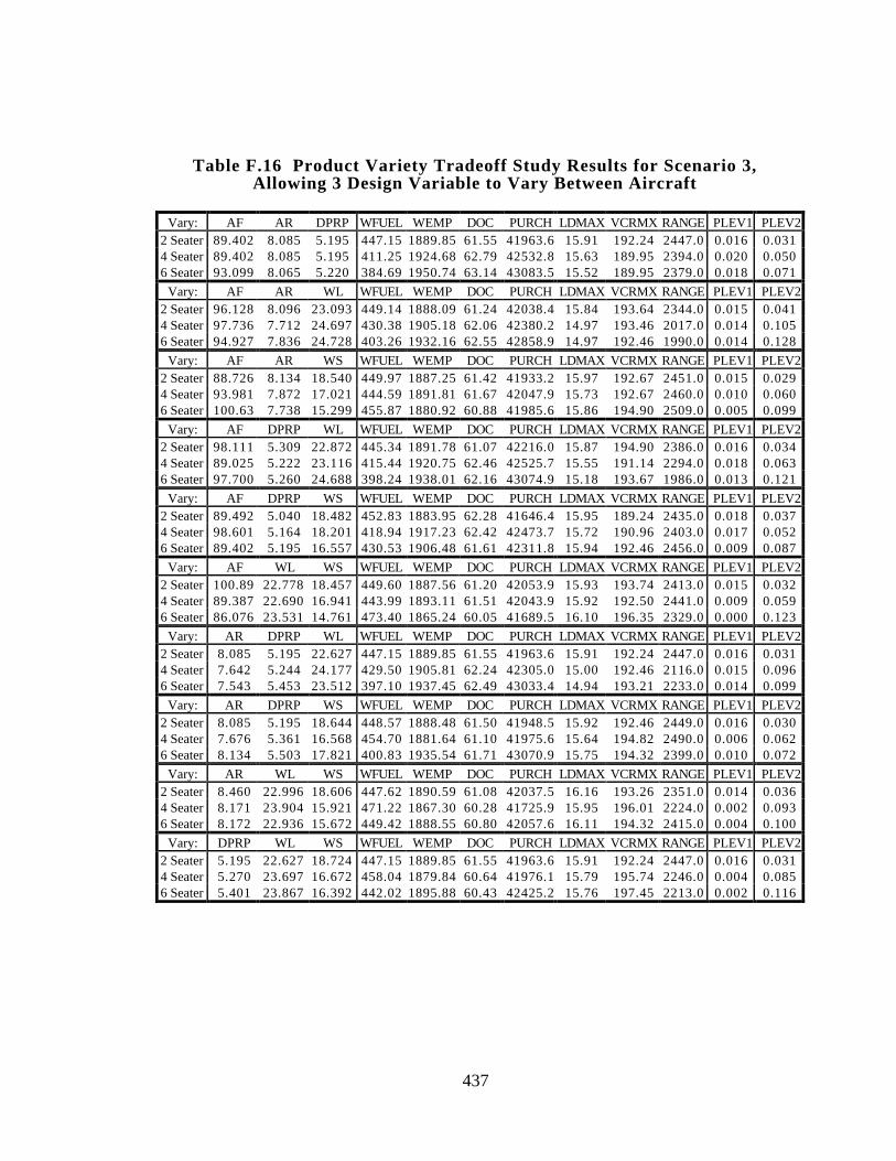
437
Table F.16 Product Variety Tradeoff Study Results for Scenario 3,Allowing 3 Design Variable to Vary Between Aircraft
Vary: AF AR DPRP WFUEL WEMP DOC PURCH LDMAX VCRMX RANGE PLEV1 PLEV22 Seater 89.402 8.085 5.195 447.15 1889.85 61.55 41963.6 15.91 192.24 2447.0 0.016 0.0314 Seater 89.402 8.085 5.195 411.25 1924.68 62.79 42532.8 15.63 189.95 2394.0 0.020 0.0506 Seater 93.099 8.065 5.220 384.69 1950.74 63.14 43083.5 15.52 189.95 2379.0 0.018 0.071
Vary: AF AR WL WFUEL WEMP DOC PURCH LDMAX VCRMX RANGE PLEV1 PLEV22 Seater 96.128 8.096 23.093 449.14 1888.09 61.24 42038.4 15.84 193.64 2344.0 0.015 0.0414 Seater 97.736 7.712 24.697 430.38 1905.18 62.06 42380.2 14.97 193.46 2017.0 0.014 0.1056 Seater 94.927 7.836 24.728 403.26 1932.16 62.55 42858.9 14.97 192.46 1990.0 0.014 0.128
Vary: AF AR WS WFUEL WEMP DOC PURCH LDMAX VCRMX RANGE PLEV1 PLEV22 Seater 88.726 8.134 18.540 449.97 1887.25 61.42 41933.2 15.97 192.67 2451.0 0.015 0.0294 Seater 93.981 7.872 17.021 444.59 1891.81 61.67 42047.9 15.73 192.67 2460.0 0.010 0.0606 Seater 100.63 7.738 15.299 455.87 1880.92 60.88 41985.6 15.86 194.90 2509.0 0.005 0.099
Vary: AF DPRP WL WFUEL WEMP DOC PURCH LDMAX VCRMX RANGE PLEV1 PLEV22 Seater 98.111 5.309 22.872 445.34 1891.78 61.07 42216.0 15.87 194.90 2386.0 0.016 0.0344 Seater 89.025 5.222 23.116 415.44 1920.75 62.46 42525.7 15.55 191.14 2294.0 0.018 0.0636 Seater 97.700 5.260 24.688 398.24 1938.01 62.16 43074.9 15.18 193.67 1986.0 0.013 0.121
Vary: AF DPRP WS WFUEL WEMP DOC PURCH LDMAX VCRMX RANGE PLEV1 PLEV22 Seater 89.492 5.040 18.482 452.83 1883.95 62.28 41646.4 15.95 189.24 2435.0 0.018 0.0374 Seater 98.601 5.164 18.201 418.94 1917.23 62.42 42473.7 15.72 190.96 2403.0 0.017 0.0526 Seater 89.402 5.195 16.557 430.53 1906.48 61.61 42311.8 15.94 192.46 2456.0 0.009 0.087
Vary: AF WL WS WFUEL WEMP DOC PURCH LDMAX VCRMX RANGE PLEV1 PLEV22 Seater 100.89 22.778 18.457 449.60 1887.56 61.20 42053.9 15.93 193.74 2413.0 0.015 0.0324 Seater 89.387 22.690 16.941 443.99 1893.11 61.51 42043.9 15.92 192.50 2441.0 0.009 0.0596 Seater 86.076 23.531 14.761 473.40 1865.24 60.05 41689.5 16.10 196.35 2329.0 0.000 0.123
Vary: AR DPRP WL WFUEL WEMP DOC PURCH LDMAX VCRMX RANGE PLEV1 PLEV22 Seater 8.085 5.195 22.627 447.15 1889.85 61.55 41963.6 15.91 192.24 2447.0 0.016 0.0314 Seater 7.642 5.244 24.177 429.50 1905.81 62.24 42305.0 15.00 192.46 2116.0 0.015 0.0966 Seater 7.543 5.453 23.512 397.10 1937.45 62.49 43033.4 14.94 193.21 2233.0 0.014 0.099
Vary: AR DPRP WS WFUEL WEMP DOC PURCH LDMAX VCRMX RANGE PLEV1 PLEV22 Seater 8.085 5.195 18.644 448.57 1888.48 61.50 41948.5 15.92 192.46 2449.0 0.016 0.0304 Seater 7.676 5.361 16.568 454.70 1881.64 61.10 41975.6 15.64 194.82 2490.0 0.006 0.0626 Seater 8.134 5.503 17.821 400.83 1935.54 61.71 43070.9 15.75 194.32 2399.0 0.010 0.072
Vary: AR WL WS WFUEL WEMP DOC PURCH LDMAX VCRMX RANGE PLEV1 PLEV22 Seater 8.460 22.996 18.606 447.62 1890.59 61.08 42037.5 16.16 193.26 2351.0 0.014 0.0364 Seater 8.171 23.904 15.921 471.22 1867.30 60.28 41725.9 15.95 196.01 2224.0 0.002 0.0936 Seater 8.172 22.936 15.672 449.42 1888.55 60.80 42057.6 16.11 194.32 2415.0 0.004 0.100
Vary: DPRP WL WS WFUEL WEMP DOC PURCH LDMAX VCRMX RANGE PLEV1 PLEV22 Seater 5.195 22.627 18.724 447.15 1889.85 61.55 41963.6 15.91 192.24 2447.0 0.016 0.0314 Seater 5.270 23.697 16.672 458.04 1879.84 60.64 41976.1 15.79 195.74 2246.0 0.004 0.0856 Seater 5.401 23.867 16.392 442.02 1895.88 60.43 42425.2 15.76 197.45 2213.0 0.002 0.116
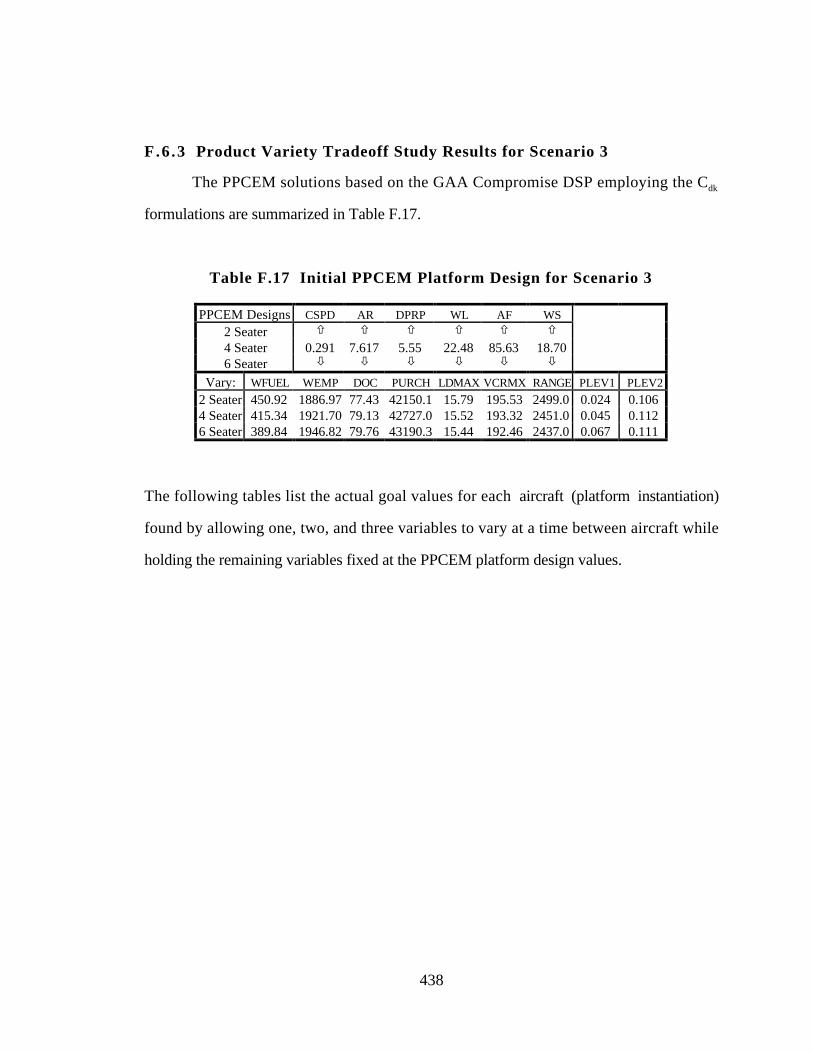
438
F.6 .3 Product Variety Tradeoff Study Results for Scenario 3
The PPCEM solutions based on the GAA Compromise DSP employing the Cdk
formulations are summarized in Table F.17.
Table F.17 Initial PPCEM Platform Design for Scenario 3
PPCEM Designs CSPD AR DPRP WL AF WS
2 Seater ñ ñ ñ ñ ñ ñ
4 Seater 0.291 7.617 5.55 22.48 85.63 18.706 Seater ò ò ò ò ò ò
Vary: WFUEL WEMP DOC PURCH LDMAX VCRMX RANGE PLEV1 PLEV2
2 Seater 450.92 1886.97 77.43 42150.1 15.79 195.53 2499.0 0.024 0.1064 Seater 415.34 1921.70 79.13 42727.0 15.52 193.32 2451.0 0.045 0.1126 Seater 389.84 1946.82 79.76 43190.3 15.44 192.46 2437.0 0.067 0.111
The following tables list the actual goal values for each aircraft (platform instantiation)
found by allowing one, two, and three variables to vary at a time between aircraft while
holding the remaining variables fixed at the PPCEM platform design values.
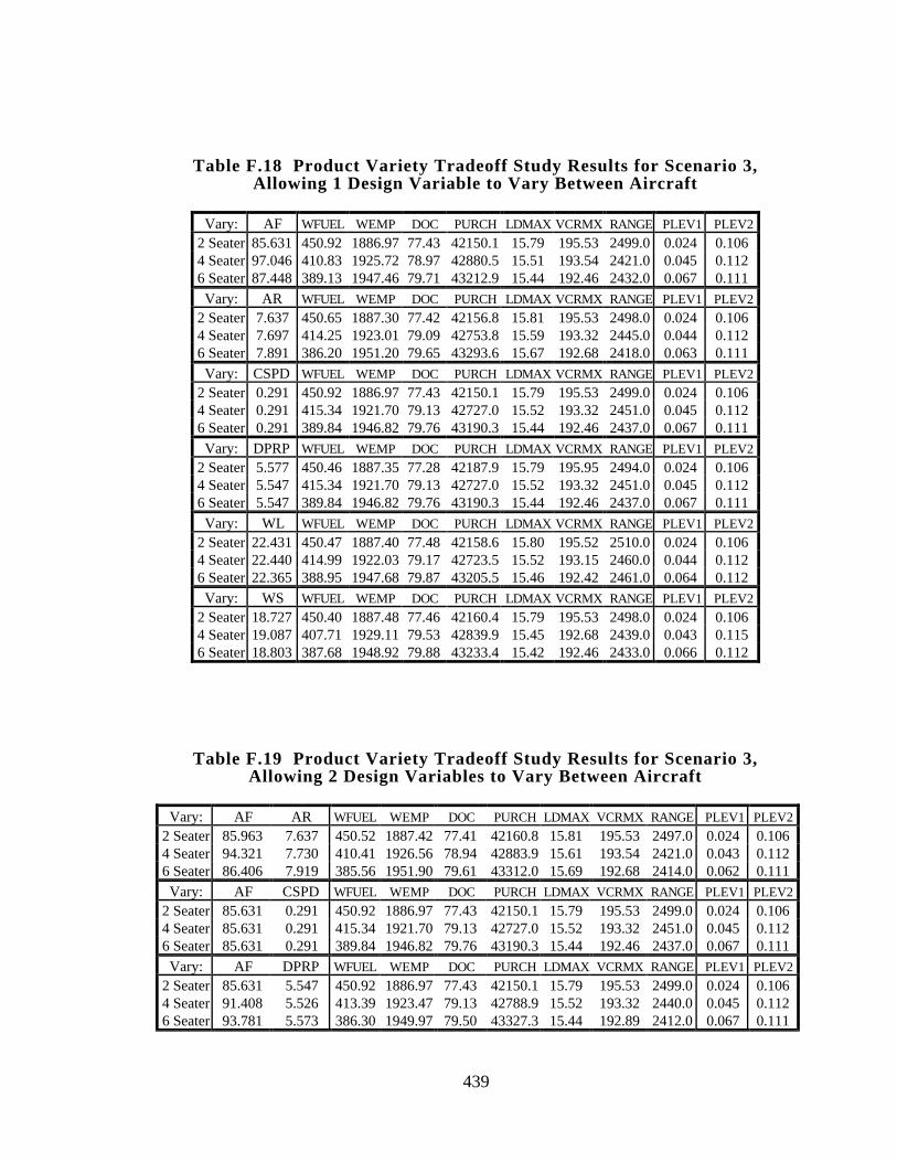
439
Table F.18 Product Variety Tradeoff Study Results for Scenario 3,Allowing 1 Design Variable to Vary Between Aircraft
Vary: AF WFUEL WEMP DOC PURCH LDMAX VCRMX RANGE PLEV1 PLEV2
2 Seater 85.631 450.92 1886.97 77.43 42150.1 15.79 195.53 2499.0 0.024 0.1064 Seater 97.046 410.83 1925.72 78.97 42880.5 15.51 193.54 2421.0 0.045 0.1126 Seater 87.448 389.13 1947.46 79.71 43212.9 15.44 192.46 2432.0 0.067 0.111
Vary: AR WFUEL WEMP DOC PURCH LDMAX VCRMX RANGE PLEV1 PLEV2
2 Seater 7.637 450.65 1887.30 77.42 42156.8 15.81 195.53 2498.0 0.024 0.1064 Seater 7.697 414.25 1923.01 79.09 42753.8 15.59 193.32 2445.0 0.044 0.1126 Seater 7.891 386.20 1951.20 79.65 43293.6 15.67 192.68 2418.0 0.063 0.111
Vary: CSPD WFUEL WEMP DOC PURCH LDMAX VCRMX RANGE PLEV1 PLEV2
2 Seater 0.291 450.92 1886.97 77.43 42150.1 15.79 195.53 2499.0 0.024 0.1064 Seater 0.291 415.34 1921.70 79.13 42727.0 15.52 193.32 2451.0 0.045 0.1126 Seater 0.291 389.84 1946.82 79.76 43190.3 15.44 192.46 2437.0 0.067 0.111
Vary: DPRP WFUEL WEMP DOC PURCH LDMAX VCRMX RANGE PLEV1 PLEV2
2 Seater 5.577 450.46 1887.35 77.28 42187.9 15.79 195.95 2494.0 0.024 0.1064 Seater 5.547 415.34 1921.70 79.13 42727.0 15.52 193.32 2451.0 0.045 0.1126 Seater 5.547 389.84 1946.82 79.76 43190.3 15.44 192.46 2437.0 0.067 0.111
Vary: WL WFUEL WEMP DOC PURCH LDMAX VCRMX RANGE PLEV1 PLEV2
2 Seater 22.431 450.47 1887.40 77.48 42158.6 15.80 195.52 2510.0 0.024 0.1064 Seater 22.440 414.99 1922.03 79.17 42723.5 15.52 193.15 2460.0 0.044 0.1126 Seater 22.365 388.95 1947.68 79.87 43205.5 15.46 192.42 2461.0 0.064 0.112
Vary: WS WFUEL WEMP DOC PURCH LDMAX VCRMX RANGE PLEV1 PLEV2
2 Seater 18.727 450.40 1887.48 77.46 42160.4 15.79 195.53 2498.0 0.024 0.1064 Seater 19.087 407.71 1929.11 79.53 42839.9 15.45 192.68 2439.0 0.043 0.1156 Seater 18.803 387.68 1948.92 79.88 43233.4 15.42 192.46 2433.0 0.066 0.112
Table F.19 Product Variety Tradeoff Study Results for Scenario 3,Allowing 2 Design Variables to Vary Between Aircraft
Vary: AF AR WFUEL WEMP DOC PURCH LDMAX VCRMX RANGE PLEV1 PLEV2
2 Seater 85.963 7.637 450.52 1887.42 77.41 42160.8 15.81 195.53 2497.0 0.024 0.1064 Seater 94.321 7.730 410.41 1926.56 78.94 42883.9 15.61 193.54 2421.0 0.043 0.1126 Seater 86.406 7.919 385.56 1951.90 79.61 43312.0 15.69 192.68 2414.0 0.062 0.111
Vary: AF CSPD WFUEL WEMP DOC PURCH LDMAX VCRMX RANGE PLEV1 PLEV2
2 Seater 85.631 0.291 450.92 1886.97 77.43 42150.1 15.79 195.53 2499.0 0.024 0.1064 Seater 85.631 0.291 415.34 1921.70 79.13 42727.0 15.52 193.32 2451.0 0.045 0.1126 Seater 85.631 0.291 389.84 1946.82 79.76 43190.3 15.44 192.46 2437.0 0.067 0.111
Vary: AF DPRP WFUEL WEMP DOC PURCH LDMAX VCRMX RANGE PLEV1 PLEV2
2 Seater 85.631 5.547 450.92 1886.97 77.43 42150.1 15.79 195.53 2499.0 0.024 0.1064 Seater 91.408 5.526 413.39 1923.47 79.13 42788.9 15.52 193.32 2440.0 0.045 0.1126 Seater 93.781 5.573 386.30 1949.97 79.50 43327.3 15.44 192.89 2412.0 0.067 0.111
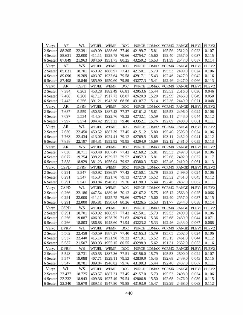
440
Vary: AF WL WFUEL WEMP DOC PURCH LDMAX VCRMX RANGE PLEV1 PLEV2
2 Seater 88.205 22.391 449.09 1888.66 77.49 42199.7 15.81 195.56 2512.0 0.023 0.1074 Seater 85.631 22.000 411.11 1925.75 79.66 42754.7 15.60 192.40 2557.0 0.037 0.1156 Seater 87.849 21.963 384.60 1951.75 80.25 43250.2 15.53 191.59 2547.0 0.057 0.114
Vary: AF WS WFUEL WEMP DOC PURCH LDMAX VCRMX RANGE PLEV1 PLEV2
2 Seater 85.631 18.701 450.92 1886.97 77.43 42150.1 15.79 195.53 2499.0 0.024 0.1064 Seater 89.090 19.209 403.97 1932.64 79.58 42917.1 15.43 192.46 2427.0 0.042 0.1166 Seater 87.408 18.846 385.90 1950.60 79.89 43277.3 15.41 192.46 2427.0 0.066 0.113
Vary: AR CSPD WFUEL WEMP DOC PURCH LDMAX VCRMX RANGE PLEV1 PLEV2
2 Seater 7.384 0.263 453.28 1882.49 66.81 42053.6 15.44 195.53 2516.0 0.030 0.0464 Seater 7.408 0.260 417.17 1917.73 68.07 42620.9 15.20 192.99 2466.0 0.049 0.0506 Seater 7.443 0.256 391.21 1943.38 68.56 43107.7 15.14 192.36 2449.0 0.071 0.048
Vary: AR DPRP WFUEL WEMP DOC PURCH LDMAX VCRMX RANGE PLEV1 PLEV2
2 Seater 7.637 5.559 450.50 1887.43 77.37 42161.2 15.81 195.53 2496.0 0.024 0.1064 Seater 7.697 5.534 414.54 1922.76 79.22 42732.1 15.59 193.11 2448.0 0.044 0.1126 Seater 7.997 5.574 384.42 1953.22 79.48 43352.1 15.76 192.89 2408.0 0.061 0.111
Vary: AR WL WFUEL WEMP DOC PURCH LDMAX VCRMX RANGE PLEV1 PLEV2
2 Seater 7.630 22.450 450.52 1887.39 77.45 42151.2 15.80 195.40 2505.0 0.024 0.1064 Seater 7.763 22.434 413.00 1924.41 79.12 42769.5 15.65 193.11 2452.0 0.041 0.1126 Seater 7.858 22.197 384.31 1952.92 79.95 43294.9 15.69 192.12 2481.0 0.055 0.113
Vary: AR WS WFUEL WEMP DOC PURCH LDMAX VCRMX RANGE PLEV1 PLEV2
2 Seater 7.638 18.711 450.48 1887.47 77.43 42160.2 15.81 195.53 2497.0 0.024 0.1064 Seater 8.077 19.254 398.23 1939.72 79.52 43057.3 15.81 192.68 2402.0 0.037 0.1176 Seater 7.888 18.929 381.23 1956.04 79.92 43380.3 15.62 192.46 2410.0 0.061 0.113
Vary: CSPD DPRP WFUEL WEMP DOC PURCH LDMAX VCRMX RANGE PLEV1 PLEV2
2 Seater 0.291 5.547 450.92 1886.97 77.43 42150.1 15.79 195.53 2499.0 0.024 0.1064 Seater 0.291 5.547 415.34 1921.70 79.13 42727.0 15.52 193.32 2451.0 0.045 0.1126 Seater 0.291 5.547 389.84 1946.82 79.76 43190.3 15.44 192.46 2437.0 0.067 0.111
Vary: CSPD WL WFUEL WEMP DOC PURCH LDMAX VCRMX RANGE PLEV1 PLEV2
2 Seater 0.266 22.186 447.54 1889.16 70.12 42167.2 15.75 195.12 2563.0 0.025 0.0664 Seater 0.291 22.000 411.11 1925.75 79.66 42754.7 15.60 192.40 2557.0 0.037 0.1156 Seater 0.291 22.000 385.81 1950.64 80.26 43226.5 15.53 191.77 2544.0 0.058 0.114
Vary: CSPD WS WFUEL WEMP DOC PURCH LDMAX VCRMX RANGE PLEV1 PLEV2
2 Seater 0.291 18.701 450.92 1886.97 77.43 42150.1 15.79 195.53 2499.0 0.024 0.1064 Seater 0.266 19.087 406.92 1928.79 71.63 42829.6 15.36 192.68 2439.0 0.044 0.0716 Seater 0.266 18.803 386.88 1948.60 71.94 43223.2 15.33 192.46 2433.0 0.067 0.068
Vary: DPRP WL WFUEL WEMP DOC PURCH LDMAX VCRMX RANGE PLEV1 PLEV2
2 Seater 5.562 22.458 450.59 1887.27 77.40 42165.3 15.79 195.65 2502.0 0.024 0.1064 Seater 5.537 22.440 415.14 1921.90 79.23 42719.1 15.52 193.15 2461.0 0.044 0.1126 Seater 5.587 21.507 380.93 1955.15 80.55 43298.9 15.62 191.31 2652.0 0.053 0.116
Vary: DPRP WS WFUEL WEMP DOC PURCH LDMAX VCRMX RANGE PLEV1 PLEV2
2 Seater 5.543 18.731 450.55 1887.36 77.51 42156.0 15.79 195.53 2500.0 0.024 0.1074 Seater 5.547 19.088 407.71 1929.11 79.53 42839.9 15.45 192.68 2439.0 0.043 0.1156 Seater 5.547 18.701 389.84 1946.82 79.76 43190.3 15.44 192.46 2437.0 0.067 0.111
Vary: WL WS WFUEL WEMP DOC PURCH LDMAX VCRMX RANGE PLEV1 PLEV2
2 Seater 22.477 18.725 450.57 1887.31 77.45 42157.0 15.79 195.53 2498.0 0.024 0.1064 Seater 22.332 18.943 409.36 1927.49 79.54 42806.8 15.50 192.68 2476.0 0.039 0.1156 Seater 22.340 18.679 389.13 1947.50 79.88 43193.9 15.47 192.29 2468.0 0.063 0.112
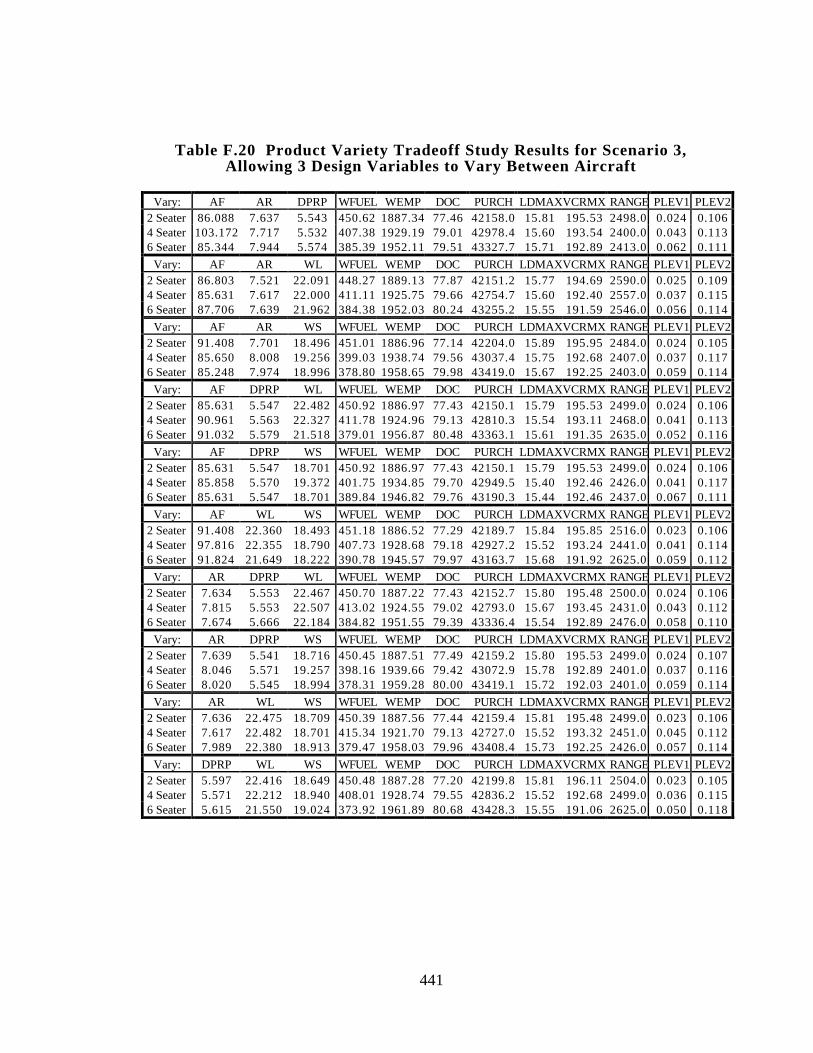
441
Table F.20 Product Variety Tradeoff Study Results for Scenario 3,Allowing 3 Design Variables to Vary Between Aircraft
Vary: AF AR DPRP WFUEL WEMP DOC PURCH LDMAXVCRMX RANGE PLEV1 PLEV22 Seater 86.088 7.637 5.543 450.62 1887.34 77.46 42158.0 15.81 195.53 2498.0 0.024 0.1064 Seater 103.172 7.717 5.532 407.38 1929.19 79.01 42978.4 15.60 193.54 2400.0 0.043 0.1136 Seater 85.344 7.944 5.574 385.39 1952.11 79.51 43327.7 15.71 192.89 2413.0 0.062 0.111
Vary: AF AR WL WFUEL WEMP DOC PURCH LDMAXVCRMX RANGE PLEV1 PLEV22 Seater 86.803 7.521 22.091 448.27 1889.13 77.87 42151.2 15.77 194.69 2590.0 0.025 0.1094 Seater 85.631 7.617 22.000 411.11 1925.75 79.66 42754.7 15.60 192.40 2557.0 0.037 0.1156 Seater 87.706 7.639 21.962 384.38 1952.03 80.24 43255.2 15.55 191.59 2546.0 0.056 0.114
Vary: AF AR WS WFUEL WEMP DOC PURCH LDMAXVCRMX RANGE PLEV1 PLEV22 Seater 91.408 7.701 18.496 451.01 1886.96 77.14 42204.0 15.89 195.95 2484.0 0.024 0.1054 Seater 85.650 8.008 19.256 399.03 1938.74 79.56 43037.4 15.75 192.68 2407.0 0.037 0.1176 Seater 85.248 7.974 18.996 378.80 1958.65 79.98 43419.0 15.67 192.25 2403.0 0.059 0.114
Vary: AF DPRP WL WFUEL WEMP DOC PURCH LDMAXVCRMX RANGE PLEV1 PLEV22 Seater 85.631 5.547 22.482 450.92 1886.97 77.43 42150.1 15.79 195.53 2499.0 0.024 0.1064 Seater 90.961 5.563 22.327 411.78 1924.96 79.13 42810.3 15.54 193.11 2468.0 0.041 0.1136 Seater 91.032 5.579 21.518 379.01 1956.87 80.48 43363.1 15.61 191.35 2635.0 0.052 0.116
Vary: AF DPRP WS WFUEL WEMP DOC PURCH LDMAXVCRMX RANGE PLEV1 PLEV22 Seater 85.631 5.547 18.701 450.92 1886.97 77.43 42150.1 15.79 195.53 2499.0 0.024 0.1064 Seater 85.858 5.570 19.372 401.75 1934.85 79.70 42949.5 15.40 192.46 2426.0 0.041 0.1176 Seater 85.631 5.547 18.701 389.84 1946.82 79.76 43190.3 15.44 192.46 2437.0 0.067 0.111
Vary: AF WL WS WFUEL WEMP DOC PURCH LDMAXVCRMX RANGE PLEV1 PLEV22 Seater 91.408 22.360 18.493 451.18 1886.52 77.29 42189.7 15.84 195.85 2516.0 0.023 0.1064 Seater 97.816 22.355 18.790 407.73 1928.68 79.18 42927.2 15.52 193.24 2441.0 0.041 0.1146 Seater 91.824 21.649 18.222 390.78 1945.57 79.97 43163.7 15.68 191.92 2625.0 0.059 0.112
Vary: AR DPRP WL WFUEL WEMP DOC PURCH LDMAXVCRMX RANGE PLEV1 PLEV22 Seater 7.634 5.553 22.467 450.70 1887.22 77.43 42152.7 15.80 195.48 2500.0 0.024 0.1064 Seater 7.815 5.553 22.507 413.02 1924.55 79.02 42793.0 15.67 193.45 2431.0 0.043 0.1126 Seater 7.674 5.666 22.184 384.82 1951.55 79.39 43336.4 15.54 192.89 2476.0 0.058 0.110
Vary: AR DPRP WS WFUEL WEMP DOC PURCH LDMAXVCRMX RANGE PLEV1 PLEV22 Seater 7.639 5.541 18.716 450.45 1887.51 77.49 42159.2 15.80 195.53 2499.0 0.024 0.1074 Seater 8.046 5.571 19.257 398.16 1939.66 79.42 43072.9 15.78 192.89 2401.0 0.037 0.1166 Seater 8.020 5.545 18.994 378.31 1959.28 80.00 43419.1 15.72 192.03 2401.0 0.059 0.114
Vary: AR WL WS WFUEL WEMP DOC PURCH LDMAXVCRMX RANGE PLEV1 PLEV22 Seater 7.636 22.475 18.709 450.39 1887.56 77.44 42159.4 15.81 195.48 2499.0 0.023 0.1064 Seater 7.617 22.482 18.701 415.34 1921.70 79.13 42727.0 15.52 193.32 2451.0 0.045 0.1126 Seater 7.989 22.380 18.913 379.47 1958.03 79.96 43408.4 15.73 192.25 2426.0 0.057 0.114
Vary: DPRP WL WS WFUEL WEMP DOC PURCH LDMAXVCRMX RANGE PLEV1 PLEV22 Seater 5.597 22.416 18.649 450.48 1887.28 77.20 42199.8 15.81 196.11 2504.0 0.023 0.1054 Seater 5.571 22.212 18.940 408.01 1928.74 79.55 42836.2 15.52 192.68 2499.0 0.036 0.1156 Seater 5.615 21.550 19.024 373.92 1961.89 80.68 43428.3 15.55 191.06 2625.0 0.050 0.118

442
F.7 SAMPLE GAA DSIDES FILES FOR PPCEM FAMILY
The following sample DSIDES files are for solving the GAA Compromise DSP
within the PPCEM. These files are explicitly for the Cdk formulation which uses the
kriging metamodels based on the 64 point orthogonal array (OA). These particular files are
for Scenario 1 with a high starting point (i.e., all design variables at their upper bound).
The .dat file is given Section F.4.1, and the . f file is given in Section F.4.2.
F.7 .1 Sample DSIDES File: gasp.oa64.cdk.s1h.dat
PTITLE : Problem Title, User Name and DatePAX=1-5,rb3l GASP; Tim Simpson and Jonathan Maier; June 18, 1998
NUMSYS : Number of system variables: real,integer,boolean 6 0 0
SYSVAR : System variable informationCSPD 1 0.24 0.48 0.48 : cruise speedAR 2 7.0 11.0 11.0 : aspect ratioDPRP 3 5.0 5.96 5.96 : propeller diameterWL 4 19.0 25.0 25.0 : wing loadingAF 5 85.0 110.0 110.0 : engine activity factorWS 6 14.0 20.0 20.0 : seat width
NUMCAG : Number of constraints and goals 0 6 0 0 7 : nlinco,nnlinq,nnlequ,nlingo,nnlgoa
ACHFUN : Achievment function 1 : level 1 7 : level 1, 7 terms (-1,0.1429) (-2,0.1429) (-3,0.1429) (-4,0.1429) (-5,0.1429) (-6,0.1429) (-7,0.1429)
STOPCR : Stopping criteria1 0 50 0.005 0.005 : perfm cal, prt intereslts, Mcyles,sta dev, sta var
NLINCO : Names of nonlinear constraintsnoise 1 : takeoff noisedoc 2 : direct operating costrough 3 : ride roughness coefficientwemp 4 : aircraft empty weightwfuel 5 : fuel weightrange 6 : minimum range
NLINGO: names of nonlinear goalswfulcd 1 : minimize fuel weight - Cdkwempcd 2 : minimize empty weight - Cdkdoccd 3 : minimize direct operating cost - Cdk

443
prchcd 4 : minimize purchase price - Cdkldmxcd 5 : maximize lift to drag ratio - Cdkmxspcd 6 : maximize max. speed - Cdkrngecd 7 : maximize range - Cdk
ALPOUT : Output Control 1 1 1 1 0 0 0 0 1 1
USRMOD : User module flags 1 1 0 0
OPTIMP : Optimization parameters -0.01 0.5 0.005 : VIOLIM, REMO, STEP
ADREMO : Using adaptive reduced move8 0.05 : Max. calls, deltaR
ENDPRB :**STOP reading the data file at this point**
F.7 .2 Sample DSIDES File: gasp.oa64.cdk.s1h.f
SUBROUTINE USRINP (NDESV,NINP,NOUT,DESVAR, & numdv,numsamp,numresp,corflag,fprefix,invmat)C*********************************************************************CC Modified call to subroutine; Tim Simpson - June 18, 1998CC Now, this subroutine does the necessary preprocessing to expediteC prediction with a kriging model; the user doesn't need to changeC anything in this routine--just make sure that it is invoked byC USRMOD in the .dat file (i.e., set first user module flag to 1)CC********************************************************************* INTEGER NDESV, NINP, NOUT REAL DESVAR(NDESV)
integer numdv,numsamp,numresp,corflag character*16 fprefix
COMMON /KRIG1/ xmat,betahat,thetaray,Rinvyfb
double precision p, invmat(numsamp,numsamp)
integer scfstr,lenstr,i,j,k,dummy,krig real dummy2 character*16 ftitle character*24 deckfile,fitsfile,scfnameCC using: maxsamp=500, maxdv=25, maxresp=20C double precision xmat(500,15),betahat(20), & thetaray(20,15),theta(15),Rinvyfb(20,500), & Fvect(500,1),FRinv(500),yvect(500),yfb_vect(500), & resp(500,20)
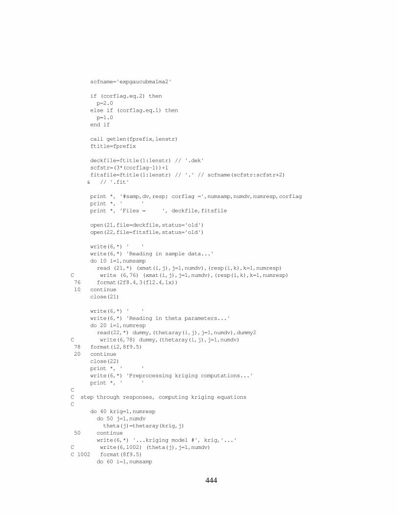
444
scfname='expgaucubma1ma2'
if (corflag.eq.2) then p=2.0 else if (corflag.eq.1) then p=1.0 end if
call getlen(fprefix,lenstr) ftitle=fprefix
deckfile=ftitle(1:lenstr) // '.dek' scfstr=(3*(corflag-1))+1 fitsfile=ftitle(1:lenstr) // '.' // scfname(scfstr:scfstr+2) & // '.fit'
print *, '#samp,dv,resp; corflag =',numsamp,numdv,numresp,corflag print *, ' ' print *, 'Files = ', deckfile,fitsfile
open(21,file=deckfile,status='old') open(22,file=fitsfile,status='old')
write(6,*) ' ' write(6,*) 'Reading in sample data...' do 10 i=1,numsamp read (21,*) (xmat(i,j),j=1,numdv),(resp(i,k),k=1,numresp)C write (6,76) (xmat(i,j),j=1,numdv),(resp(i,k),k=1,numresp) 76 format(2f8.4,3(f12.4,1x)) 10 continue close(21)
write(6,*) ' ' write(6,*) 'Reading in theta parameters...' do 20 i=1,numresp read(22,*) dummy,(thetaray(i,j),j=1,numdv),dummy2C write(6,78) dummy,(thetaray(i,j),j=1,numdv) 78 format(i2,8f9.5) 20 continue close(22) print *, ' ' write(6,*) 'Preprocessing kriging computations...' print *, ' 'CC step through responses, computing kriging equationsC do 40 krig=1,numresp do 50 j=1,numdv theta(j)=thetaray(krig,j) 50 continue write(6,*) '...kriging model #', krig,'...'C write(6,1002) (theta(j),j=1,numdv)C 1002 format(8f9.5) do 60 i=1,numsamp
445
yvect(i)=resp(i,krig) Fvect(i,1)=1.0d0 60 continue
call cormat (xmat,invmat,numsamp,numdv, & theta,p,corflag) call compeqn (invmat,Fvect,yvect,FRinv,yfb_vect, & Rinvyfb,betahat,numsamp,numdv,krig)CC increment variable krig to look at next responseC 40 continue
RETURN ENDCC subroutine to parse filename specified in ‘dace.params.h’ file.C subroutine getlen(string,lenstr) character*1 blank character*16 string parameter (blank=' ') integer next,lenstr do 10 next = LEN(string), 1, -1 if (string(next:next).ne.blank) then lenstr=next return end if 10 continue lenstr=0 if (lenstr.eq.0) then write(6,*) 'You have not specified a file name prefix' stop end if return endCC subroutine needed for kriging metamodel computationC subroutine cormat (xmat,invmat,numsamp,numdv,theta,p,corflag) integer numdv,numsamp,corflag,ipvt(500) double precision xmat(500,15),invmat(numsamp,numsamp), & work(500),p,theta(15) integer i,j,info double precision det(2),R
do 300 i = 1,numsamp do 305 j = i,numsamp if( i .eq. j ) then invmat(i,j) = 1.0d0 else call scfxmat(R,xmat,theta,corflag,p,numdv,numsamp,i,j) invmat(i,j) = R invmat(j,i) = invmat(i,j) endif
446
305 continue 300 continue
C do 306 i=1,numsampC write(6,82) (invmat(i,j),j=1,numsamp)C 82 format(14(f4.2,1x))C 306 continue
do 307 i=1,numsamp work(i)=0.0d0 ipvt(i)=0 307 continue call dgefa(invmat, numsamp, numsamp, ipvt, info) if( info .ne. 0 ) then write(*,*)"Error in DGEFA, info = ",info stop endif call dgedi(invmat, numsamp, numsamp, ipvt, det, work, 11)
C do 310 i=1,numsampC write(6,84) (invmat(i,j),j=1,numsamp)C 84 format(14(f10.2,1x))C 310 continue
return end************************************************************************* include LINPACK routines used to find inverse of correlation matrix************************************************************************* include 'dgefa.f' include 'dgedi.f'************************************************************************CC subroutine needed for kriging metamodel computationC subroutine compeqn (invmat,Fvect,yvect,FRinv,yfb_vect, & Rinvyfb,betahat,numsamp,numdv,krig)
integer numsamp,numdv double precision betahat(20),invmat(numsamp,numsamp), & Fvect(500,1),FRinv(500), & Rinvyfb(20,500),yvect(500),yfb_vect(500) double precision beta_den,beta_num integer i,j,krigCC compute F'RinvC do 310 i=1,numsamp FRinv(i)=0.0d0 do 315 j=1,numsamp FRinv(i)=FRinv(i)+Fvect(j,1)*invmat(j,i)
447
315 continue 310 continueCC compute betahat = (F'Rinv*yvect)/(F'Rinv*F)C beta_den=0.0d0 beta_num=0.0d0 do 320 i=1,numsamp beta_den=beta_den+FRinv(i)*Fvect(i,1) beta_num=beta_num+FRinv(i)*yvect(i) 320 continue betahat(krig) = beta_num / beta_denCC compute y-f'betahatC do 330 i = 1,numsamp yfb_vect(i) = yvect(i) - betahat(krig)*Fvect(i,1) 330 continueCC compute Rinv*(y-f'beta)C do 340 i=1,numsamp Rinvyfb(krig,i)=0.0d0 do 345 j=1,numsamp Rinvyfb(krig,i)=Rinvyfb(krig,i)+invmat(i,j)*yfb_vect(j) 345 continue 340 continue return end
CC subroutine needed for kriging metamodel computationC subroutine scfxmat(R,xmat,theta,corflag,p,numdv,numsamp,i,j) integer i,j,corflag,numdv,numsamp double precision R,xmat(500,15),theta(15),p double precision sum,thetadist,dist integer k
if ((corflag.eq.2).or.(corflag.eq.1)) then sum=0.0d0 do 120 k = 1,numdv dist = DABS(xmat(i,k)-xmat(j,k)) sum = sum + theta(k)*((dist)**p) 120 continue R = DEXP( -1.0d0*sum ) else if (corflag.eq.3) then sum=1.0d0 do 130 k=1,numdv dist = ABS(xmat(i,k)-xmat(j,k)) thetadist=dist*theta(k) if (thetadist.lt.0.5) then sum=sum*(1.0-6.0*(thetadist**2)+6.0*(thetadist**3)) else if (thetadist.ge.1.0) then sum=sum*0.0
448
else sum=sum*(2.0*(1.0-thetadist)**3) end if 130 continue R = sum else if (corflag.eq.4) then sum=1.0 do 140 k=1,numdv dist = ABS(xmat(i,k)-xmat(j,k)) sum = sum*(exp(-theta(k)*dist)*(1.+theta(k)*dist)) 140 continue R = sum else if (corflag.eq.5) then sum=1.0 do 150 k=1,numdv dist = ABS(xmat(i,k)-xmat(j,k)) thetadist=dist*theta(k) sum = sum*(exp(-thetadist)* & (1.+thetadist+(thetadist**2)/3.0)) 150 continue R = sum end if
return endC*********************************************************************C SUBROUTINE USROUT (NDESV, NOUT, DESVAR, LCONDF, LCONSV, LXFEAS)CC Tim Simpson - June 18, 1998CC This subroutine postprocesses the solution by taking the finalC converged values and instantiating each aircraft in GASP. TheC resulting deviation function is computed for each aircraft asC specified by the variable ‘iscen’. After processing, a file calledC ‘gasp.oa64.cdk.s1h.mod’ is created which containts all of theC necessary information for each instantiation. (The output fileC name can be changed by changing variable ‘outfile’.CC********************************************************************* INTEGER NDESV, NOUT REAL DESVAR(NDESV) LOGICAL LCONDF, LCONSV, LXFEASC CHARACTER*80 LINE
INTEGER NUM, IPARAMETER (NUM=7)CHARACTER*10 CHGVAR(NUM)REAL CHGVAL(NUM)INTEGER CHRLEN(NUM), INDEXinteger INLINE,NUMOUT,nscaleparameter(NUMOUT=11,nscale=3)REAL NOISE,WEMP,DOC,ROUGH,WFUEL,PURCH,VCRMX,LDMAX,RANGE
REAL RESPONSE(NUMOUT,nscale),GOALS(7,nscale),
449
& dplus(7,nscale),dminus(7,nscale),devfcn(4,nscale), & convio(nscale),CONSTR(6,nscale)
real noisec(nscale),tpspdc(nscale),docc(nscale), & roughc(nscale),wempc(nscale),wfuelc(nscale), & wfuelt(nscale),wempt(nscale),doct(nscale), & ldmaxt(nscale),vcrmxt(nscale),ranget(nscale), & purcht(nscale),rangec(nscale)
integer ipax REAL xlo(6),xhi(6),xnew(6) REAL EMCRU,AR,DPROP,WGS,AF,WS,PAX integer j,i,iscen character*28 outfile
data xlo / 0.24, 7.0, 5.0, 19.0, 85.0, 14.0 / data xhi / 0.48, 11.0, 5.96, 25.0, 110.0, 20.0 /CC define array of constraints for each response for each aircraftC data noisec / 75., 75., 75. / data tpspdc / 850., 850., 850. / data docc / 80., 80., 80. / data roughc / 2., 2., 2. / data wempc / 2200., 2200., 2200. / data wfuelc / 450., 475., 500. / data rangec / 2000., 2000., 2000. /CC define array of goal targets for each response for each aircraftC data wfuelt / 450., 400., 350. / data wempt / 1900., 1950., 2000. / data doct / 60., 60., 60. / data purcht / 41000., 42000., 43000. / data ldmaxt / 17., 17., 17. / data vcrmxt / 200., 200., 200. / data ranget / 2500., 2500., 2500. /
iscen=1 outfile='gasp.oa64.cdk.s1h.mod' open(unit=27,file=outfile,status='unknown')
EMCRU = DESVAR(1) AR = DESVAR(2) DPROP = DESVAR(3) WGS = DESVAR(4) AF = DESVAR(5) WS = DESVAR(6)CC scale the design variables to [0,1] - necessary for krigingC do 10 j=1,6 xnew(j)=(DESVAR(j)-xlo(j))/(xhi(j)-xlo(j)) 10 continue
write(6,*) ' ' write(6,*) outfile
450
write(6,*) ' ' write(6,*) 'Instantiate final values in GASP:' write(6,*) ' ' write(6,*) ' INPUTS: Act. Value Scaled Value' write(6,73) 73 format(3(12('-'),1x)) write(6,74) 'Cruise_Spd=',EMCRU,xnew(1) write(6,74) 'Aspct_Rtio=',AR,xnew(2) write(6,74) 'Prop_Diamr=',DPROP,xnew(3) write(6,74) 'Wing_Loadg=',WGS,xnew(4) write(6,74) 'Eng_Act_Fc=',AF,xnew(5) write(6,74) 'Seat_Width=',WS,xnew(6) 74 format(A12,1x,f12.4,1x,f12.4)CC write instantiations to output fileC write(27,*) ' ' write(27,*) outfile write(27,*) ' ' write(27,*) 'Instantiate final values in GASP:' write(27,*) ' ' write(27,*) ' INPUTS: Act. Value Scaled Value' write(27,73) write(27,74) 'Cruise_Spd=',EMCRU,xnew(1) write(27,74) 'Aspct_Rtio=',AR,xnew(2) write(27,74) 'Prop_Diamr=',DPROP,xnew(3) write(27,74) 'Wing_Loadg=',WGS,xnew(4) write(27,74) 'Eng_Act_Fc=',AF,xnew(5) write(27,74) 'Seat_Width=',WS,xnew(6)CC specify number of passengersC do 300 ipax=1,3 PAX = (2.*REAL(ipax))-1C***********************************************************************C USER has to redifine the following block to create GASP input fileC*********************************************************************** CHGVAR(1) = 'EMCRU'
CHRLEN(1) = 5CHGVAL(1) = EMCRU
CHGVAR(2) = 'AR'CHRLEN(2) = 2CHGVAL(2) = AR
CHGVAR(3) = 'DPROP'CHRLEN(3) = 5CHGVAL(3) = DPROPCHGVAR(4) = 'WGS'CHRLEN(4) = 3CHGVAL(4) = WGS
CHGVAR(5) = 'AF' CHRLEN(5) = 2 CHGVAL(5) = AF CHGVAR(6) = 'WS' CHRLEN(6) = 2 CHGVAL(6) = WS
451
CHGVAR(7) = 'PAX' CHRLEN(7) = 3 CHGVAL(7) = PAX
C**********************************************************************C user doesn't have to change anything in the following blockC*********************************************************************CC create GASP input file: GASP.INC OPEN(UNIT=100,FILE='GASPINPUT.rb3l') call system('rm GASP.IN') OPEN(UNIT=110,FILE='GASP.IN',STATUS='NEW') DO WHILE ( .TRUE. ) READ(100,70,END=1000) LINE
INDEX = INLINE(NUM, LINE, CHGVAR, CHRLEN, CHGVAL)IF (INDEX .NE. 0) THEN
WRITE(110, 75) CHGVAR(INDEX)(1:CHRLEN(INDEX)), + CHGVAL(INDEX) ELSE WRITE(110,70) LINE
END IF 70 FORMAT ( A80) 75 FORMAT (2X, A, '=', F10.2, ',') ENDDO1000 CONTINUE CLOSE(100) CLOSE(110)CC execute GASP with current values of design variablesC CALL SYSTEM('rm performance') call system('rm GASP.OUT') print *, ' ' print *, 'Executing GASP for Passenger #',PAX CALL SYSTEM('gasp <GASP.IN>GASP.OUT') PRINT *, '' PRINT *, 'GASP IS DONE'CC read GASP output file named performance into response arrayC OPEN(UNIT=120,FILE='performance', STATUS='UNKNOWN') DO 200 I =1, NUMOUT READ (120, *) RESPONSE(I,ipax)200 CONTINUE CLOSE(120)300 continue write(6,*) ' ' write(6,*) ' OUTPUTS: 1 Pax 3 Pax 5 Pax' write(6,77) 77 format(4(12('-'),1x)) write(6,78) 'Noise=', (RESPONSE(2,j),j=1,3) write(6,78) 'Empty_Wgt=', (RESPONSE(3,j),j=1,3) write(6,78) 'Oper_Cost=', (RESPONSE(5,j),j=1,3) write(6,78) 'Ride_Rough=', (RESPONSE(6,j),j=1,3)
452
write(6,78) 'Fuel_Wgt=', (RESPONSE(7,j),j=1,3) write(6,78) 'Purch_Price=', (RESPONSE(8,j),j=1,3) write(6,78) 'Max_Range=', (RESPONSE(9,j),j=1,3) write(6,78) 'Max_Speed=', (RESPONSE(10,j),j=1,3) write(6,78) 'L/D_Max=', (RESPONSE(11,j),j=1,3) 78 format(A12,1x,f12.4,1x,f12.4,1x,f12.4) write(6,*) ' 'CC write instantiations to fileC write(27,*) ' ' write(27,*) ' OUTPUTS: 1 Pax 3 Pax 5 Pax' write(27,77) write(27,78) 'Noise=', (RESPONSE(2,j),j=1,3) write(27,78) 'Empty_Wgt=', (RESPONSE(3,j),j=1,3) write(27,78) 'Oper_Cost=', (RESPONSE(5,j),j=1,3) write(27,78) 'Ride_Rough=', (RESPONSE(6,j),j=1,3) write(27,78) 'Fuel_Wgt=', (RESPONSE(7,j),j=1,3) write(27,78) 'Purch_Price=', (RESPONSE(8,j),j=1,3) write(27,78) 'Max_Range=', (RESPONSE(9,j),j=1,3) write(27,78) 'Max_Speed=', (RESPONSE(10,j),j=1,3) write(27,78) 'L/D_Max=', (RESPONSE(11,j),j=1,3) write(27,*) ' 'CC compute deviation function for each aircraftC do 310 j=1,3
NOISE = RESPONSE(2,j) WEMP = RESPONSE(3,j) DOC = RESPONSE(5,j) ROUGH = RESPONSE(6,j) WFUEL = RESPONSE(7,j) PURCH = RESPONSE(8,j) RANGE = RESPONSE(9,j) VCRMX = RESPONSE(10,j) LDMAX = RESPONSE(11,j)
GOALS(1,j) = WFUEL/wfuelt(j)-1.0 GOALS(2,j) = WEMP/wempt(j) - 1.0 GOALS(3,j) = DOC/doct(j) - 1.0 GOALS(4,j) = PURCH/purcht(j) - 1.0 GOALS(5,j) = LDMAX/ldmaxt(j) - 1.0 GOALS(6,j) = VCRMX/vcrmxt(j) - 1.0 GOALS(7,j) = RANGE/ranget(j) - 1.0
do 320 i=1,7 if(GOALS(i,j).ge.0)then dplus(i,j)=ABS(GOALS(i,j)) dminus(i,j)=0.0 else dplus(i,j)=0.0 dminus(i,j)=ABS(GOALS(i,j)) endif 320 continue
453
if(iscen.eq.1)then devfcn(1,j)=(dplus(1,j)+dplus(2,j)+dplus(3,j)+dplus(4,j)+ & dminus(5,j)+dminus(6,j)+dminus(7,j))/7. devfcn(2,j)=0.0 devfcn(3,j)=0.0 devfcn(4,j)=0.0
else if(iscen.eq.2) then devfcn(1,j)=(dplus(2,j)+dplus(3,j)+dplus(4,j))/3. devfcn(2,j)=(dplus(1,j)+dminus(5,j)+ & dminus(6,j)+dminus(7,j))/4. devfcn(3,j)=0.0 devfcn(4,j)=0.0
else if(iscen.eq.3) then devfcn(1,j)=(dplus(1,j)+dminus(5,j)+ & dminus(6,j)+dminus(7,j))/4. devfcn(2,j)=(dplus(2,j)+dplus(3,j)+dplus(4,j))/3. devfcn(3,j)=0.0 devfcn(4,j)=0.0
else if(iscen.eq.4) then devfcn(1,j)=(dplus(2,j)+dplus(4,j))/2. devfcn(2,j)=dplus(3,j) devfcn(3,j)=(dplus(1,j)+dminus(5,j)+ & dminus(6,j)+dminus(7,j))/4. devfcn(4,j)=0.0
else if(iscen.eq.5) then devfcn(1,j)=dplus(3,j) devfcn(2,j)=(dplus(2,j)+dplus(4,j))/2. devfcn(3,j)=(dplus(1,j)+dminus(5,j)+ & dminus(6,j)+dminus(7,j))/4. devfcn(4,j)=0.0
else if(iscen.eq.6) then devfcn(1,j)=(dplus(1,j)+dminus(6,j))/2. devfcn(2,j)=(dminus(5,j)+dminus(6,j))/2. devfcn(3,j)=(dplus(2,j)+dplus(3,j)+dplus(4,j))/3. devfcn(4,j)=0.0
else if(iscen.eq.7) then devfcn(1,j)=dminus(5,j) devfcn(2,j)=dminus(7,j) devfcn(3,j)=(dplus(1,j)+dminus(6,j))/2. devfcn(4,j)=(dplus(2,j)+dplus(3,j)+dplus(4,j))/3.
else if(iscen.eq.8) then devfcn(1,j)=dminus(7,j) devfcn(2,j)=dminus(5,j) devfcn(3,j)=(dplus(1,j)+dminus(6,j))/2. devfcn(4,j)=(dplus(2,j)+dplus(3,j)+dplus(4,j))/3.
endif
454
310 continue
write(6,78) 'P_lev_1=', (devfcn(1,j),j=1,3) if(iscen.ge.2) then write(6,78) 'P_lev_2=', (devfcn(2,j),j=1,3) if(iscen.ge.4) then write(6,78) 'P_lev_3=', (devfcn(3,j),j=1,3) if(iscen.ge.7) then write(6,78) 'P_lev_4=', (devfcn(4,j),j=1,3) end if end if end ifCC write instantiations to fileC write(27,78) 'P_lev_1=', (devfcn(1,j),j=1,3) if(iscen.ge.2) then write(27,78) 'P_lev_2=', (devfcn(2,j),j=1,3) if(iscen.ge.4) then write(27,78) 'P_lev_3=', (devfcn(3,j),j=1,3) if(iscen.ge.7) then write(27,78) 'P_lev_4=', (devfcn(4,j),j=1,3) end if end if end ifCC compute constraint violationC do 410 j=1,3
NOISE = RESPONSE(2,j) WEMP = RESPONSE(3,j) DOC = RESPONSE(5,j) ROUGH = RESPONSE(6,j) WFUEL = RESPONSE(7,j) RANGE = RESPONSE(9,j)
CONSTR(1,j) = 1.0 - NOISE/noisec(j) CONSTR(2,j) = 1.0 - DOC/docc(j) CONSTR(3,j) = 1.0 - ROUGH/roughc(j) CONSTR(4,j) = 1.0 - WEMP/wempc(j) CONSTR(5,j) = 1.0 - WFUEL/wfuelc(j) CONSTR(6,j) = RANGE/rangec(j) - 1.0
convio(j)=0.0 do 420 i=1,6 if(CONSTR(i,j).lt.0.0)then convio(j)=convio(j)+ABS(CONSTR(i,j)) end if 420 continue 410 continue
write(6,*) ' ' write(6,78) 'Con_Vio=',(convio(j),j=1,3)
455
write(6,*) ' ' write(27,*) ' ' write(27,78) 'Con_Vio=',(convio(j),j=1,3) write(27,*) ' '
close(27)
RETURN ENDC*********************************************************************C user does not need to change the following function blockC********************************************************************** FUNCTION INLINE(NUM, LINE, CHGVAR, CHRLEN, CHGVAL)
INTEGER INLINE, NUM, ICHARACTER*80 LINECHARACTER*10 CHGVAR(NUM)
INTEGER CHRLEN(NUM)REAL CHGVAL(NUM)
DO 10 I = 1, NUMIF (LINE(3:3+CHRLEN(I)) .EQ. CHGVAR(I)(1:CHRLEN(I))
+ //'=') THENINLINE = IGOTO 20END IF
10 CONTINUEINLINE = 0
20 ENDC***********************************************************************CC Subroutine USRSETCC Purpose: Evaluate non-linear constraints and goals.C NOTE - Do not specify the deviation variablesCC-----------------------------------------------------------------------C Arguments Name Type DescriptionC --------- ---- ---- -----------C Input: IPATH int = 1 evaluate constraints and goalsC = 2 evaluate constraints onlyC = 3 evaluate goals onlyC NDESV int number of design variablesC MNLNCG int maximum number of nonlinearC constraints and goalsC NOUT int unit number of output data fileC DESVAR real vector of design variablesCC Output: CONSTR real vector of constraint valuesC GOALS real vector of goal valuesCC Input/Output: noneC-----------------------------------------------------------------------C Common Blocks: noneC
456
C Include Files: noneCC Called from: GCALCCC Calls to: noneC-----------------------------------------------------------------------C Development HistoryCC Author: BHARAT PATELC Date: 13 MARCH, 1992.CC Modifications:CC***********************************************************************CC SUBROUTINE USRSET (IPATH, NDESV, MNLNCG, NOUT, DESVAR, & CONSTR, GOALS)CC------------------------------C Passed variables from RUNALPC------------------------------C INTEGER IPATH, NDESV, MNLNCG, NOUTC REAL DESVAR(NDESV) REAL CONSTR(MNLNCG), GOALS(MNLNCG) INTEGER VVNUMCC------------------------------------------------C Variables particular to kriging implementationC------------------------------------------------C COMMON /KRIG1/ xmat,betahat,thetaray,Rinvyfb COMMON /KRIG2/ nmdv,nmsamp,nmresp,corfcn double precision xmat(500,15),betahat(20), & thetaray(20,15),Rinvyfb(20,500) integer nmdv,nmsamp,nmresp,corfcn integer j,krig double precision ynew(20),xnew(15),theta(15), & R,r_xhat(500),yevalCC---------------------------------------------C Local variables particular to c-dsp problemC---------------------------------------------C REAL xlo(6),xhi(6) REAL EMCRU,AR,DPROP,WGS,AF,WS, & NOISEm,WEMPm,DOCm,ROUGHm,WFUELm, & PURCHm,VCRMXm,LDMAXm,RANGEm, & NOISEv,WEMPv,DOCv,ROUGHv,WFUELv, & PURCHv,VCRMXv,LDMAXv,RANGEv, & NOISEcd,NOISEcdu,ROUGHcd,ROUGHcdu, & VCRMXcdl,LDMAXcdl,RANGEcdl, & VCRMXcd,LDMAXcd,RANGEcd,
457
& WFUELcd,WFUELcdu,WFUELcdl, & WEMPcd,WEMPcdu,WEMPcdl, & PURCHcd,PURCHcdu,PURCHcdl, & DOCcd,DOCcdu
data xlo / 0.24, 7.0, 5.0, 19.0, 85.0, 14.0 / data xhi / 0.48, 11.0, 5.96, 25.0, 110.0, 20.0 /
EMCRU = DESVAR(1) AR = DESVAR(2) DPROP = DESVAR(3) WGS = DESVAR(4) AF = DESVAR(5) WS = DESVAR(6)CC scale the design variables to [0,1] - necessary for krigingC do 10 j=1,nmdv xnew(j)=(DESVAR(j)-xlo(j))/(xhi(j)-xlo(j)) 10 continue
VVNUM=VVNUM+1
PRINT *, ' ' PRINT *, ' INPUTS: Act. Value Scaled Value Run#',VVNUM write(6,73) 73 format(3(12('-'),1x)) write(6,74) 'Cruise_Spd=',EMCRU,xnew(1) write(6,74) 'Aspct_Rtio=',AR,xnew(2) write(6,74) 'Prop_Diamr=',DPROP,xnew(3) write(6,74) 'Wing_Loadg=',WGS,xnew(4) write(6,74) 'Eng_Act_Fc=',AF,xnew(5) write(6,74) 'Seat_Width=',WS,xnew(6) 74 format(A12,1x,f12.4,1x,f12.4)
C*********************************************************************CC kriging prediction block; Tim Simpson - June 18, 1998C *user does not have to change anything in this block*CC********************************************************************* do 40 krig=1,nmrespCC transfer theta parameters for current response (designated by krig)C do 50 j=1,nmdv theta(j)=thetaray(krig,j) 50 continueCC compute correlation vector for xnewC do 60 j=1,nmsamp call scfxnew(R,xnew,xmat,theta,corfcn,nmdv,nmsamp,j) r_xhat(j)=R 60 continue
458
CC calculate ynew of current responseC yeval = 0.0d0 do 220 j=1,nmsamp 220 yeval=yeval+r_xhat(j)*Rinvyfb(krig,j) ynew(krig) = yeval + betahat(krig)CC increment variable krig to predict next ynewC 40 continueCC equate predicted ynew vector to appropriate responsesC NOISEm = REAL(ynew(1)) WEMPm = REAL(ynew(2)) DOCm = REAL(ynew(3)) ROUGHm = REAL(ynew(4)) WFUELm = REAL(ynew(5)) PURCHm = REAL(ynew(6)) RANGEm = REAL(ynew(7)) VCRMXm = REAL(ynew(8)) LDMAXm = REAL(ynew(9)) NOISEv = REAL(ynew(10)) WEMPv = REAL(ynew(11)) DOCv = REAL(ynew(12)) ROUGHv = REAL(ynew(13)) WFUELv = REAL(ynew(14)) PURCHv = REAL(ynew(15)) RANGEv = REAL(ynew(16)) VCRMXv = REAL(ynew(17)) LDMAXv = REAL(ynew(18))CC compute Cdk valuesC NOISEcdu=(75.-NOISEm)/(NOISEv*(3.**0.5)) NOISEcd=NOISEcdu
ROUGHcdu=(2.00-ROUGHm)/(ROUGHv*(3.**0.5)) ROUGHcd=ROUGHcdu
DOCcdu=(60.-DOCm)/(DOCv*(3.**0.5)) DOCcd=DOCcdu
WEMPcdl=(WEMPm-1900.)/(WEMPv*(3.**0.5)) WEMPcdu=(2000.-WEMPm)/(WEMPv*(3.**0.5)) WEMPcd=AMIN1(WEMPcdl,WEMPcdu)
WFUELcdl=(WFUELm-350.)/(WFUELv*(3.**0.5)) WFUELcdu=(450.-WFUELm)/(WFUELv*(3.**0.5)) WFUELcd=AMIN1(WFUELcdl,WFUELcdu)
PURCHcdl=(PURCHm-41000.)/(PURCHv*(3.**0.5)) PURCHcdu=(43000.-PURCHm)/(PURCHv*(3.**0.5)) PURCHcd=AMIN1(PURCHcdu,PURCHcdl)
459
VCRMXcdl=(VCRMXm-200.0)/(VCRMXv*(3.**0.5)) VCRMXcd=VCRMXcdl
RANGEcdl=(RANGEm-2500.0)/(RANGEv*(3.**0.5)) RANGEcd=RANGEcdl
LDMAXcdl=(LDMAXm-17.0)/(LDMAXv*(3.**0.5)) LDMAXcd=LDMAXcdlCC print out corresponding values of constraint and goal responseC PRINT *, ' ' PRINT *, ' OUTPUTS: Mean Variance Cdk' write(6,77) 77 format(4(12('-'),1x)) write(6,78) 'Noise=', NOISEm, NOISEv, NOISEcd write(6,78) 'Empty_Wgt=', WEMPm, WEMPv, WEMPcd write(6,78) 'Oper_Cost=',DOCm, DOCv, DOCcd write(6,78) 'Ride_Rough=', ROUGHm, ROUGHv, ROUGHcd write(6,78) 'Fuel_Wgt=', WFUELm, WFUELv, WFUELcd write(6,78) 'Purch_Price=', PURCHm, PURCHv, PURCHcd write(6,78) 'Max_Range=', RANGEm, RANGEv, RANGEcd write(6,78) 'Max_Speed=', VCRMXm, VCRMXv, VCRMXcd write(6,78) 'L/D_Max=', LDMAXm, LDMAXv, LDMAXcd 78 format(A12,1x,f12.4,1x,f12.4,1x,f12.5) print *, ' 'CC 3.0 Evaluate non-linear constraintsC IF (IPATH .EQ. 1 .OR. IPATH .EQ. 2) THENCC constraint formulations for restricting appropriate Cdk >= 1C CONSTR(1) = NOISEcd - 1.0 CONSTR(2) = (80.-DOCm)/(DOCv*(3.**0.5)) - 1.0 CONSTR(3) = ROUGHcd - 1.0 CONSTR(4) = (2200.-WEMPm)/(WEMPv*(3.**0.5)) - 1.0 CONSTR(5) = (450.-WFUELm)/(WFUELv*(3.**0.5)) - 1.0 CONSTR(6) = (RANGEm-2000.)/(RANGEv*(3.**0.5)) - 1.0 END IFCC 4.0 Evaluate non-linear goalsC IF (IPATH .EQ. 1 .OR. IPATH .EQ. 3) THENCC specify goals; want all Cdk >= 1.C GOALS(1) = WFUELcd-1.0 GOALS(2) = WEMPcd - 1.0 GOALS(3) = DOCcd - 1.0 GOALS(4) = PURCHcd - 1.0 GOALS(5) = LDMAXcd - 1.0 GOALS(6) = VCRMXcd - 1.0 GOALS(7) = RANGEcd - 1.0
460
END IFCC 5.0 Return to calling routineC RETURN ENDCC subroutine needed for kriging metamodel computation to compute correlationC between sample points and new prediction pointC subroutine scfxnew(R,xnew,xmat,theta,corfcn,nmdv,nmsamp,j) integer j,corfcn,nmdv,nmsamp double precision R,xnew(15), & xmat(500,15),theta(15) double precision sum,thetadist,dist,p integer k
if ((corfcn.eq.2).or.(corfcn.eq.1)) then if(corfcn.eq.2)then p=2. else p=1. endif
sum=0.0d0 do 400 k = 1,nmdv dist = ABS(xnew(k)-xmat(j,k)) sum = sum + theta(k)*((dist)**p) 400 continue R = exp( -1.0d0*sum ) else if (corfcn.eq.3) then sum=1.0d0 do 410 k=1,nmdv dist = ABS(xnew(k)-xmat(j,k)) thetadist=theta(k)*dist if (thetadist.lt.0.5) then sum=sum*(1.0-6.0*(thetadist**2)+6.0*(thetadist**3)) else if (thetadist.ge.1.0) then sum=sum*0.0 else sum=sum*(2.0*(1.0-thetadist)**3) end if 410 continue R = sum else if (corfcn.eq.4) then sum=1.0 do 420 k=1,nmdv dist = ABS(xnew(k)-xmat(j,k)) sum = sum*(exp(-theta(k)*dist)*(1.+theta(k)*dist)) 420 continue R = sum else if (corfcn.eq.5) then sum=1.0 do 430 k=1,nmdv
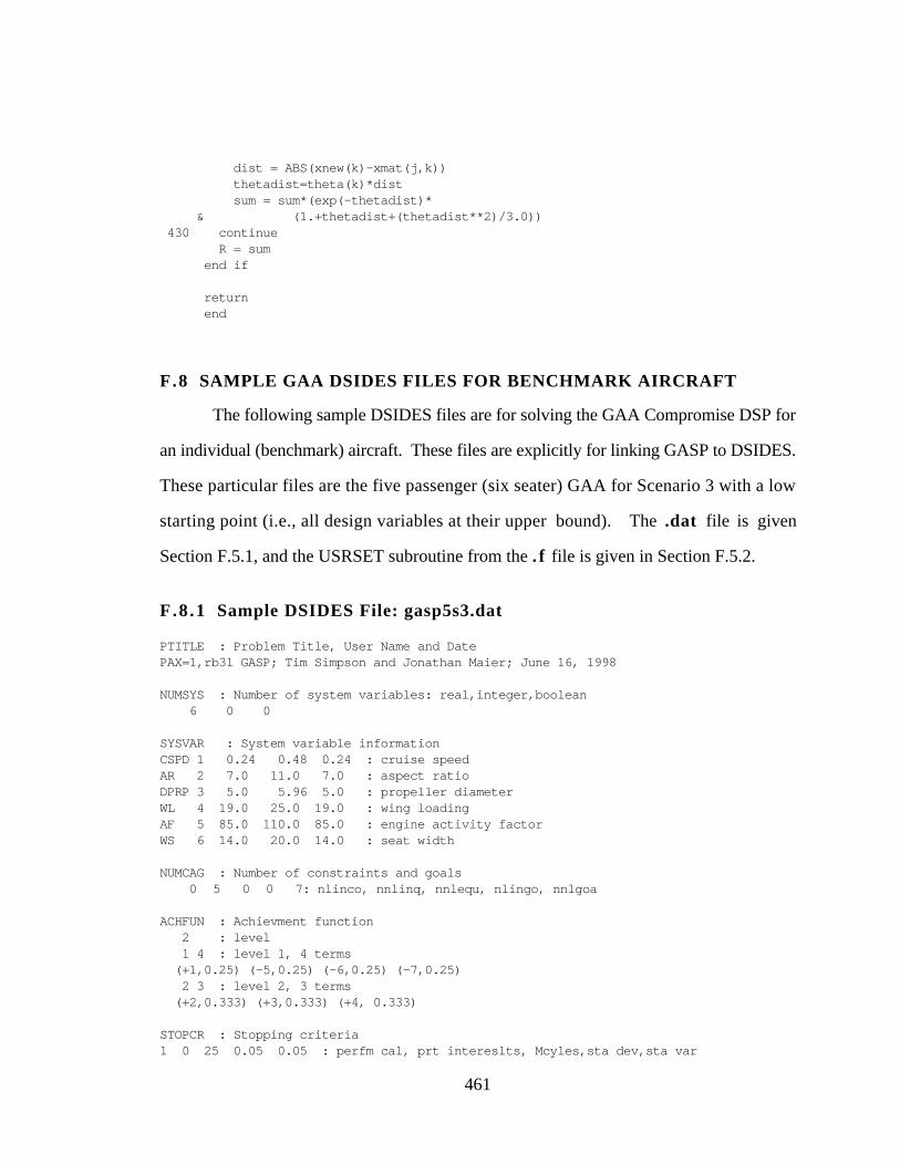
461
dist = ABS(xnew(k)-xmat(j,k)) thetadist=theta(k)*dist sum = sum*(exp(-thetadist)* & (1.+thetadist+(thetadist**2)/3.0)) 430 continue R = sum end if
return end
F.8 SAMPLE GAA DSIDES FILES FOR BENCHMARK AIRCRAFT
The following sample DSIDES files are for solving the GAA Compromise DSP for
an individual (benchmark) aircraft. These files are explicitly for linking GASP to DSIDES.
These particular files are the five passenger (six seater) GAA for Scenario 3 with a low
starting point (i.e., all design variables at their upper bound). The .dat file is given
Section F.5.1, and the USRSET subroutine from the . f file is given in Section F.5.2.
F.8 .1 Sample DSIDES File: gasp5s3.dat
PTITLE : Problem Title, User Name and DatePAX=1,rb3l GASP; Tim Simpson and Jonathan Maier; June 16, 1998
NUMSYS : Number of system variables: real,integer,boolean 6 0 0
SYSVAR : System variable informationCSPD 1 0.24 0.48 0.24 : cruise speedAR 2 7.0 11.0 7.0 : aspect ratioDPRP 3 5.0 5.96 5.0 : propeller diameterWL 4 19.0 25.0 19.0 : wing loadingAF 5 85.0 110.0 85.0 : engine activity factorWS 6 14.0 20.0 14.0 : seat width
NUMCAG : Number of constraints and goals 0 5 0 0 7: nlinco, nnlinq, nnlequ, nlingo, nnlgoa
ACHFUN : Achievment function 2 : level 1 4 : level 1, 4 terms (+1,0.25) (-5,0.25) (-6,0.25) (-7,0.25) 2 3 : level 2, 3 terms (+2,0.333) (+3,0.333) (+4, 0.333)
STOPCR : Stopping criteria1 0 25 0.05 0.05 : perfm cal, prt intereslts, Mcyles,sta dev,sta var
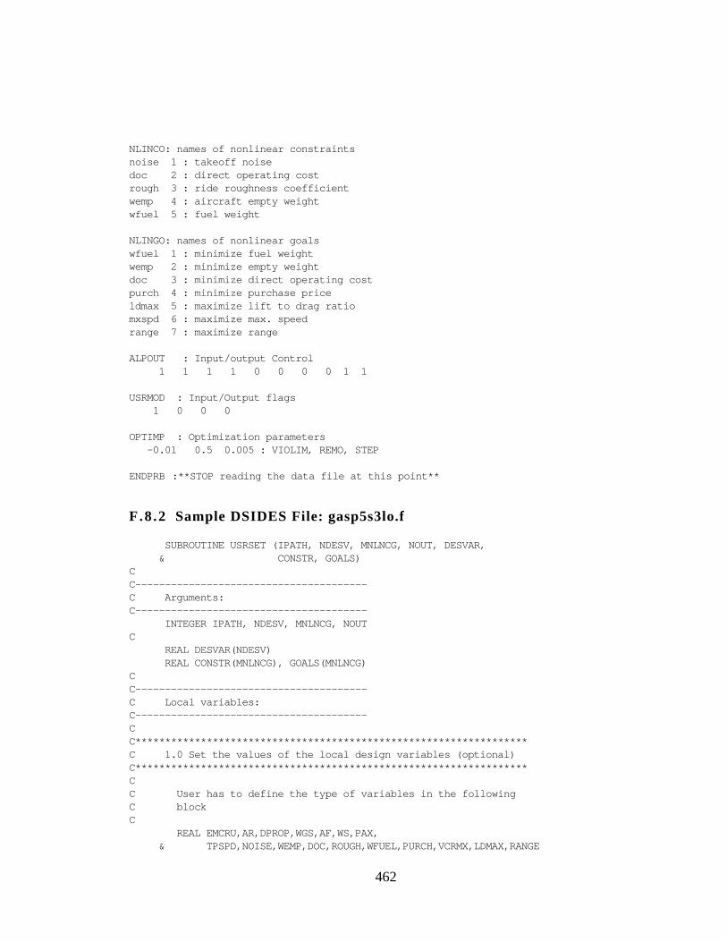
462
NLINCO: names of nonlinear constraintsnoise 1 : takeoff noisedoc 2 : direct operating costrough 3 : ride roughness coefficientwemp 4 : aircraft empty weightwfuel 5 : fuel weight
NLINGO: names of nonlinear goalswfuel 1 : minimize fuel weightwemp 2 : minimize empty weightdoc 3 : minimize direct operating costpurch 4 : minimize purchase priceldmax 5 : maximize lift to drag ratiomxspd 6 : maximize max. speedrange 7 : maximize range
ALPOUT : Input/output Control 1 1 1 1 0 0 0 0 1 1
USRMOD : Input/Output flags 1 0 0 0
OPTIMP : Optimization parameters -0.01 0.5 0.005 : VIOLIM, REMO, STEP
ENDPRB :**STOP reading the data file at this point**
F.8 .2 Sample DSIDES File: gasp5s3lo.f
SUBROUTINE USRSET (IPATH, NDESV, MNLNCG, NOUT, DESVAR, & CONSTR, GOALS)CC---------------------------------------C Arguments:C--------------------------------------- INTEGER IPATH, NDESV, MNLNCG, NOUTC REAL DESVAR(NDESV) REAL CONSTR(MNLNCG), GOALS(MNLNCG)CC---------------------------------------C Local variables:C---------------------------------------CC******************************************************************C 1.0 Set the values of the local design variables (optional)C******************************************************************CC User has to define the type of variables in the followingC blockC REAL EMCRU,AR,DPROP,WGS,AF,WS,PAX, & TPSPD,NOISE,WEMP,DOC,ROUGH,WFUEL,PURCH,VCRMX,LDMAX,RANGE
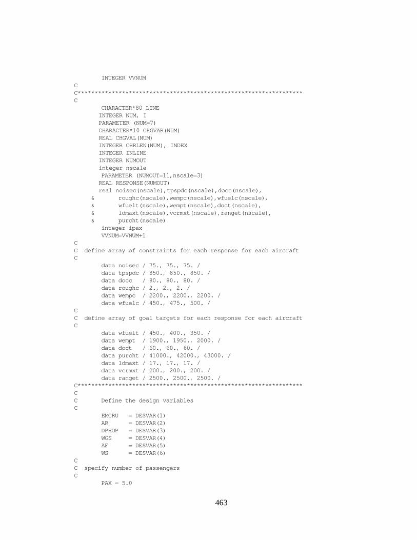
463
INTEGER VVNUMCC******************************************************************C CHARACTER*80 LINE
INTEGER NUM, IPARAMETER (NUM=7)CHARACTER*10 CHGVAR(NUM)REAL CHGVAL(NUM)INTEGER CHRLEN(NUM), INDEXINTEGER INLINEINTEGER NUMOUTinteger nscale
PARAMETER (NUMOUT=11,nscale=3)REAL RESPONSE(NUMOUT)real noisec(nscale),tpspdc(nscale),docc(nscale),
& roughc(nscale),wempc(nscale),wfuelc(nscale), & wfuelt(nscale),wempt(nscale),doct(nscale), & ldmaxt(nscale),vcrmxt(nscale),ranget(nscale), & purcht(nscale) integer ipax VVNUM=VVNUM+1CC define array of constraints for each response for each aircraftC data noisec / 75., 75., 75. / data tpspdc / 850., 850., 850. / data docc / 80., 80., 80. / data roughc / 2., 2., 2. / data wempc / 2200., 2200., 2200. / data wfuelc / 450., 475., 500. /CC define array of goal targets for each response for each aircraftC data wfuelt / 450., 400., 350. / data wempt / 1900., 1950., 2000. / data doct / 60., 60., 60. / data purcht / 41000., 42000., 43000. / data ldmaxt / 17., 17., 17. / data vcrmxt / 200., 200., 200. / data ranget / 2500., 2500., 2500. /C******************************************************************CC Define the design variablesC EMCRU = DESVAR(1) AR = DESVAR(2) DPROP = DESVAR(3) WGS = DESVAR(4) AF = DESVAR(5) WS = DESVAR(6)CC specify number of passengersC PAX = 5.0
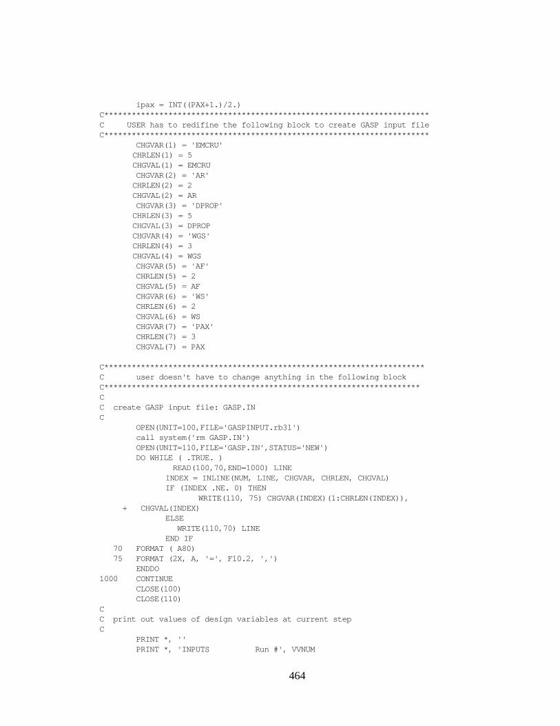
464
ipax = INT((PAX+1.)/2.)C***********************************************************************C USER has to redifine the following block to create GASP input fileC*********************************************************************** CHGVAR(1) = 'EMCRU'
CHRLEN(1) = 5CHGVAL(1) = EMCRU
CHGVAR(2) = 'AR'CHRLEN(2) = 2CHGVAL(2) = AR
CHGVAR(3) = 'DPROP'CHRLEN(3) = 5CHGVAL(3) = DPROPCHGVAR(4) = 'WGS'CHRLEN(4) = 3CHGVAL(4) = WGS
CHGVAR(5) = 'AF' CHRLEN(5) = 2 CHGVAL(5) = AF CHGVAR(6) = 'WS' CHRLEN(6) = 2 CHGVAL(6) = WS CHGVAR(7) = 'PAX' CHRLEN(7) = 3 CHGVAL(7) = PAX
C**********************************************************************C user doesn't have to change anything in the following blockC*********************************************************************CC create GASP input file: GASP.INC OPEN(UNIT=100,FILE='GASPINPUT.rb3l') call system('rm GASP.IN') OPEN(UNIT=110,FILE='GASP.IN',STATUS='NEW') DO WHILE ( .TRUE. ) READ(100,70,END=1000) LINE
INDEX = INLINE(NUM, LINE, CHGVAR, CHRLEN, CHGVAL)IF (INDEX .NE. 0) THEN
WRITE(110, 75) CHGVAR(INDEX)(1:CHRLEN(INDEX)), + CHGVAL(INDEX) ELSE WRITE(110,70) LINE
END IF 70 FORMAT ( A80) 75 FORMAT (2X, A, '=', F10.2, ',') ENDDO1000 CONTINUE CLOSE(100) CLOSE(110)CC print out values of design variables at current stepC PRINT *, '' PRINT *, 'INPUTS Run #', VVNUM
465
PRINT *, '' print *, 'Cruise_Spd=',EMCRU PRINT *, 'Aspct_Rtio=',AR PRINT *, 'Prop_Diamr=',DPROP print *, 'Wing_Loadg=',WGS print *, 'Eng_Act_Fc=',AF print *, 'Seat_Width=',WSCC execute GASP with current values of design variablesC CALL SYSTEM('rm performance') call system('rm GASP.OUT') CALL SYSTEM('gasp <GASP.IN>GASP.OUT') PRINT *, '' PRINT *, 'GASP IS DONE'CC read GASP output file named performance into response arrayC OPEN(UNIT=120,FILE='performance', STATUS='UNKNOWN') DO 200 I =1, NUMOUT READ (120, *) RESPONSE(I)200 CONTINUE
CLOSE(120)CC equate response array values to goal and constraint variables;C response(4) in performance file is SFC which is not usedC TPSPD = RESPONSE(1) NOISE = RESPONSE(2) WEMP = RESPONSE(3) DOC = RESPONSE(5) ROUGH = RESPONSE(6) WFUEL = RESPONSE(7) PURCH = RESPONSE(8) RANGE = RESPONSE(9) VCRMX = RESPONSE(10) LDMAX = RESPONSE(11)CC print out corresponding values of constraint and goal responseC PRINT *, '' PRINT *, 'OUTPUTS' PRINT *, '' PRINT *, 'Tipspd=', TPSPD, ' Noise=', NOISE PRINT *, 'Empty Wgt=', WEMP, ' Oper Cost=',DOC PRINT *, 'Ride Rough=', ROUGH, ' Max Range=', RANGE PRINT *, 'Fuel Wgt=', WFUEL, ' Purch Price=', PURCH PRINT *, 'Max Speed=', VCRMX, ' L/D Max=', LDMAXCC*************************************************************************C 3.0 Evaluate non-linear constraintsC**************************************************************************C IF (IPATH .EQ. 1 .OR. IPATH .EQ. 2) THEN
466
CC specify constraints; all constraints are less than constraintsC CONSTR(1) = 1.0 - NOISE/noisec(ipax) CONSTR(2) = 1.0 - DOC/docc(ipax) CONSTR(3) = 1.0 - ROUGH/roughc(ipax) CONSTR(4) = 1.0 - WEMP/wempc(ipax) CONSTR(5) = 1.0 - WFUEL/wfuelc(ipax)
END IFCC**************************************************************************C 4.0 Evaluate non-linear goalsC************************************************************************** IF (IPATH .EQ. 1 .OR. IPATH .EQ. 3) THENCC specify goalsC GOALS(1) = WFUEL/wfuelt(ipax)-1.0 GOALS(2) = WEMP/wempt(ipax) - 1.0 GOALS(3) = DOC/doct(ipax) - 1.0 GOALS(4) = PURCH/purcht(ipax) - 1.0 GOALS(5) = LDMAX/ldmaxt(ipax) - 1.0 GOALS(6) = VCRMX/vcrmxt(ipax) - 1.0 GOALS(7) = RANGE/ranget(ipax) - 1.0
END IFCC 5.0 Return to calling routineC RETURN ENDC*********************************************************************C user does not need to change the following function blockC********************************************************************** FUNCTION INLINE(NUM, LINE, CHGVAR, CHRLEN, CHGVAL)
INTEGER INLINE, NUM, ICHARACTER*80 LINECHARACTER*10 CHGVAR(NUM)
INTEGER CHRLEN(NUM)REAL CHGVAL(NUM)DO 10 I = 1, NUM
IF (LINE(3:3+CHRLEN(I)) .EQ. CHGVAR(I)(1:CHRLEN(I)) + //'=') THEN
INLINE = IGOTO 20END IF
10 CONTINUEINLINE = 0
20 END
467
REFERENCES
1982, The Concise Oxford Dictionary, Oxford University Press, Oxford, UK.
Abair, R., 1995, October 22-27, "Agile Manufacturing: This Is not Just Repackaging ofMaterial Requirements Planning and Just-In-Time," 38th American Production andInventory Control Society (APICS) International Conference and Exhibition,Orlando, FL, APICS, pp. 196-198.
Alexander, B., 1993, June 14-16, "Kodak Fun Saver Camera Recycling," Society ofPlastics Engineers Recycling Conference - Survival Tactics thru the '90's, Chicago,IL, pp. 207-212.
Alexandrov, N., Dennis, J. E., Jr., Lewis, R. M. and Torczon, V., 1997, "A TrustRegion Framework for Managing the Use of Approximation Models inOptimization," NASA/CR-20145, ICASE Report. No. 97-50, Institute forComputer Applications in Science and Engineering (ICASE), NASA LangleyResearch Center, Hampton, VA.
Anderson, D. M. and Pine, B. J., II, 1997, Agile Product Development for MassCustomization, Irwin, Chicago, IL.
Arora, J. S., 1989, Introduction to Optimum Design, McGraw-Hill, New York.
Balling, R. J. and Clark, D. T., 1992, September 21-23, "A Flexible ApproximationModel for Use with Optimization," 4th AIAA/USAF/NASA/OAI Symposium onMultidisciplinary Analysis and Optimization, Cleveland, OH, AIAA, Vol. 2, pp.886-894. AIAA-92-4801-CP.
Barton, R. R., 1992, December 13-16, "Metamodels for Simulation Input-OutputRelations," Proceedings of the 1992 Winter Simulation Conference (Swain, J. J.,Goldsman, D., et al., eds.), Arlington, VA, IEEE, pp. 289-299.
Barton, R. R., 1994, December 11-14, "Metamodeling: A State of the Art Review,"Proceedings of the 1994 Winter Simulation Conference (Tew, J. D., Manivannan,S., et al., eds.), Lake Beuna Vista, FL, IEEE, pp. 237-244.
Bond, A. H. and Ricci, R. J., 1992, "Cooperation in Aircraft Design," Research inEngineering Design, Vol. 4, pp. 115-130.
Booker, A. J., 1996, "Case Studies in Design and Analysis of Computer Experiments,"Proceedings of the Section on Physical and Engineering Sciences, AmericanStatistical Association.
Booker, A. J., Conn, A. R., Dennis, J. E., Frank, P. D., Serafini, D., Torczon, V. andTrosset, M., 1996, "Multi-Level Design Optimization: A Boeing/IBM/Rice
468
Collaborative Project," 1996 Final Report, ISSTECH-96-031, The BoeingCompany, Seattle, WA.
Booker, A. J., Conn, A. R., Dennis, J. E., Frank, P. D., Trosset, M. and Torczon, V.,1995, "Global Modeling for Optimization: Boeing/IBM/Rice Collaborative Project,"1995 Final Report, ISSTECH-95-032, The Boeing Company, Seattle, WA.
Box, G. E. P. and Behnken, D. W., 1960, "Some New Three Level Designs for the Studyof Quantitative Variables," Technometrics, Vol. 2, No. 4, pp. 455-475, "Errata,"Vol. 3, No. 4, p. 576.
Box, G. E. P. and Draper, N. R., 1987, Empirical Model Building and ResponseSurfaces, John Wiley & Sons, New York.
Box, M. J. and Draper, N. R., 1971, "Factorial Designs, the |X'X| Criterion, and SomeRelated Matters," Technometrics, Vol. 13, No. 4 (November), pp. 731-742.
Bras, B. A. and Mistree, F., 1991, "Designing Design Processes in Decision-BasedConcurrent Engineering," SAE Transactions, Journal of Materials &Manufacturing, SAE International, Warrendale, PA, pp. 451-458.
Byrne, D. M. and Taguchi, S., 1987, "The Taguchi Approach to Parameter Design,"Quality Progress, Vol. December, pp. 19-26.
Chaloner, K. and Verdinelli, I., 1995, "Bayesian Experimental Design: A Review,"Statistical Science, Vol. 10, No. 3, pp. 273-304.
Chambers, J. M., Freeny, A. E. and Heiberger, R. M., 1992, "Chapter 5: Analysis ofVariance; Designed Experiments," Statistical Models in S (Chambers, J. M. andHastie, T. J., eds.), Wadsworth & Brooks/Cole, Pacific Grove, CA, pp. 145-193.
Chang, T.-S. and Ward, A. C., 1995, September 17-20, "Design-in-Modularity withConceptual Robustness," Advances in Design Automation (Azarm, S., Dutta, D.,et al., eds.), Boston, MA, ASME, Vol. 82-1, pp. 493-500.
Chang, T.-S., Ward, A. C., Lee, J. and Jacox, E. H., 1994, November 6-11, "DistributedDesign with Conceptual Robustness: A Procedure Based on Taguchi's ParameterDesign," Concurrent Product Design Conference (Gadh, R., ed.), Chicago, IL,ASME, Vol. 74, pp. 19-29.
Chapman, S. J., 1991, Electric Machinery Fundamentals, McGraw-Hill, New York.
Chen, W., Rosen, D., Allen, J. K. and Mistree, F., 1994, "Modularity and theIndependence of Functional Requirements in Designing Complex Systems,"Concurrent Product Design (Gadh, R., ed.), ASME, Vol. 74, pp. 31-38.
Chen, W., 1995, "A Robust Complex Exploration Method for Configuring ComplexSystems," Ph.D. Dissertation, G. W. Woodruff School of MechanicalEngineering, Georgia Institute of Technology, Atlanta, GA.
469
Chen, W., Allen, J. K., Mavris, D. and Mistree, F., 1996a, "A Concept ExplorationMethod for Determining Robust Top-Level Specifications," EngineeringOptimization, Vol. 26, No. 2, pp. 137-158.
Chen, W., Allen, J. K., Tsui, K.-L. and Mistree, F., 1996b, "A Procedure for RobustDesign: Minimizing Variations Caused by Noise and Control Factors," Journal ofMechanical Design, Vol. 118, No. 4, pp. 478-485.
Chen, W., Simpson, T. W., Allen, J. K. and Mistree, F., 1996c, August 18-22, "Use ofDesign Capability Indices to Satisfy a Ranged Set of Design Requirements,"Advances in Design Automation (Dutta, D., ed.), Irvine, CA, ASME, Paper No.96-DETC/DAC-1090.
Chen, W., Allen, J. K., Schrage, D. P. and Mistree, F., 1997, "StatisticalExperimentation Methods for Achieving Affordable Concurrent Systems Design,"AIAA Journal, Vol. 35, No. 5, pp. 893-900.
Chen, W., Allen, J. K. and Mistree, F., 1997, "A Robust Concept Exploration Method forEnhancing Productivity in Concurrent Systems Design," Concurrent Engineering:Research and Applications, Vol. 5, No. 3, pp. 203-217.
Cheng, B. and Titterington, D. M., 1994, "Neural Networks: A Review from a StatisticalPerspective," Statistical Science, Vol. 9, No. 1, pp. 2-54.
Chinnaiah, P. S. S., Kamarthi, S. V. and Cullinane, T. P., 1998, "Characterization andAnalysis of Mass-Customized Production Systems," International Journal of AgileManufacturing, under review.
Clark, K. B. and Wheelwright, S. C., 1993, Managing New Product and ProcessDevelopment, Free Press, New York.
Cogdell, J. R., 1996, Foundations of Electrical Engineering, Prentice Hall, Upper SaddleRiver, NJ.
Collier, D. A., 1981, "The Measurement and Operating Benefits of Component PartCommonality," Decision Sciences, Vol. 12, No. 1, pp. 85-96.
Collier, D. A., 1982, "Aggregate Safety Stock Levels and Component Part Commonality,"Management Science, Vol. 28, No. 22, pp. 1296-1303.
Cox, D. D. and John, S., 1995, March 13-16, "SDO: A Statistical Method for GlobalOptimization," Proceedings of the ICASE/NASA Langley Workshop onMultidisciplinary Optimization (Alexandrov, N. M. and Hussaini, M. Y., eds.),Hampton, VA, SIAM, pp. 315-329.
Cressie, N. A. C., 1993, Statistics for Spatial Data, Revised Edition, John Wiley & Sons,New York.
Currin, C., Mitchell, T., Morris, M. and Ylvisaker, D., 1991, "Bayesian Prediction ofDeterministic Functions, With Applications to the Design and Analysis of Computer
470
Experiments," Journal of the American Statistical Association, Vol. 86, No. 416,pp. 953-963.
Davis, S. M., 1987, Future Perfect, Addison-Wesley Publishing Company, Reading, MA.
Dennis, J. E. and Torczon, V., 1995, March 13-16, "Managing Approximation Models inOptimization," Proceedings of the ICASE/NASA Langley Workshop onMultidisciplinary Design Optimization (Alexandrov, N. M. and Hussaini, M. Y.,eds.), Hampton, VA, SIAM, pp. 330-347.
Dennis, J. E., Jr. and Torczon, V., 1996, September 4-6, "Approximation ModelManagement for Optimization," 6th AIAA/USAF/NASA/ISSMO Symposium onMultidisciplinary Analysis and Optimization, Bellevue, WA, AIAA, Vol. 2, pp.1044-1046. AIAA-96-4099-CP.
Dhumal, A., Dhawan, R., Kona, A. and Soni, A. H., 1996, August 18-22,"Reconfigurable System Analysis for Agile Manufacturing," 5th ASME FlexibleAssembly Conference (Soni, A., ed.), Irvine, CA, ASME, Paper No. 96-DETC/FAS-1367.
DiCamillo, G. T., 1988, "Winning Turnaround Strategies at Black & Decker," Journal ofBusiness Strategy, Vol. 9, No. 2, pp. 30-33.
Diwekar, U. M., 1995, "Hammersley Sampling Sequence (HSS) Manual," Engineering &Public Policy Department, Carnegie Mellon University, Pittsburgh, PA.
Eggert, R. J. and Mayne, R. W., 1993, "Probabilistic Optimal Design Using SuccessiveSurrogate Probability Density Functions," Journal of Mechanical Design, Vol. 115,No. 3, pp. 385-391.
Erens, F. and Breuls, P., 1995, "Structuring Product Families in the DevelopmentProcess," Proceedings of ASI'95, Lisbon, Portugal, .
Erens, F. and Verhulst, K., 1997, "Architectures for Product Families," Computers inIndustry, Vol. 33, No. 165-178, pp.
Erens, F. J. and Hegge, H. M. H., 1994, "Manufacturing and Sales Co-ordination forProduct Variety," International Journal of Production Economics, Vol. 37, No. 1,pp. 83-99.
Erens, F., 1997, "Synthesis of Variety: Developing Product Families," Ph.D. Dissertation,University of Technology, Eindhoven, The Netherlands.
Fang, K.-T. and Wang, Y., 1994, Number-theoretic Methods in Statistics, Chapman &Hall, New York.
Finger, S. and Dixon, J. R., 1989a, "A Review of Research in Mechanical EngineeringDesign. Part 1: Descriptive, Prescriptive, and Computer-Based Models of DesignProcesses," Research in Engineering Design, Vol. 1, pp. 51-67.
471
Finger, S. and Dixon, J. R., 1989b, "A Review of Research in Mechanical EngineeringDesign. Part 2: Representations, Analysis, and Design for the Life Cycle,"Research in Engineering Design, Vol. 1, pp. 121-137.
Fujita, K. and Ishii, K., 1997, September 14-17, "Task Structuring TowardComputational Approaches to Product Variety Design," Advances in DesignAutomation (Dutta, D., ed.), Sacramento, CA, ASME, Paper No. DETC97/DAC-3766.
G.S. Electric, 1997, "Why Universal Motors Turn On the Appliance Industry,"http://www.gselectric.com/electric/univers4.htm.
Giovannitti-Jensen, A. and Myers, R. H., 1989, "Graphical Assessment of the PredictionCapability of Response Surface Designs," Technometrics, Vol. 31, No. 2 (May),pp. 159-171.
Giunta, A. A., 1997, "Aircraft Multidisciplinary Design Optimization Using Design ofExperiments Theory and Response Surface Modeling," Ph.D. Dissertation andMAD Center Report No. 97-05-01, Department of Aerospace and OceanEngineering, Virginia Polytechnic Institute and State University, Blacksburg, VA.
Giunta, A. A., Dudley, J. M., Narducci, R., Grossman, B., Haftka, R. T., Mason, W.H. and Watson, L. T., 1994, September 7-9, "Noisy Aerodynamic Response andSmooth Approximations in HSCT Design," 5th AIAA/USAF/NASA/ISSMOSymposium on Multidisciplinary Analysis and Optimization, Panama City, FL,AIAA, Vol. 2, pp. 1117-1128. AIAA-94-4376-CP.
Giunta, A., Watson, L. T. and Koehler, J., 1998, September 2-4, "A Comparison ofApproximation Modeling Techniques: Polynomial Versus Interpolating Models,"7th AIAA/USAF/NASA/ISSMO Symposium on Multidisciplinary Analysis &Optimization, St. Louis, MI, AIAA, AIAA-98-4758.
Goffe, W. L., Ferrier, G. D. and Rogers, J., 1994, "Global Optimization of StatisticalFunctions with Simulated Annealing," Journal of Econometrics, Vol. 60, No. 1-2,pp. 65-100. Source code is available at http://netlib2.cs.utk.edu/opt.
Goldberg, D. E., 1989, Genetic Algorithms in Search, Optimization, and MachineLearning, Addison-Wesley Publishing Company, Inc., New York.
Hagemann, G., Schley, C.-A., Odintsov, E. and Sobatchkine, A., 1996, July, "NozzleFlowfield Analysis with Particular Regard to 3D-Plug-Cluster Configurations,"AIAA-96-2954.
Hajela, P. and Berke, L., 1992, "Neural Networks in Structural Analysis and Design: AnOverview," Computing Systems in Engineering, Vol. 3, No. 1-4, pp. 525-538.
Hardin, R. H. and Sloane, N. J. A., 1993, "A New Approach to the Construction ofOptimal Designs," Journal of Statistical Planning and Inference, Vol. 37, pp. 339-369.
472
Hernandez, G., 1998, "A Probablistic-Based Design Approach with Game TheoreticalRepresentations of the Enterprise Design Process," M.S. Thesis, G. W. WoodruffSchool of Mechanical Engineering, Georgia Institute of Technology, Atlanta, GA.
Hernandez, G., Simpson, T. W., Allen, J. K., Bascaran, E., Avila, L. F. and Salinas, F.,1998, September 13-16, "Robust Design of Product Families for Make-to-OrderSystems," Advances in Design Automation Conference, Atlanta, GA, ASME,DETC98/DAC-5595.
Hollins, B. and Pugh, S., 1990, Successful Product Design, Butterworths, Boston, MA.
Hormozi, A., 1994, October 30-November 4, "Agile Manufacturing," 37th AmericanProduction and Inventory Control Society (APICS) International Conference andExhibition, San Diego, CA, APICS, pp. 216-218.
Hubka, V. and Eder, W. E., 1988, Theory of Technical Systems: A Total Concept Theoryfor Engineering Design, Springer, New York.
Hubka, V. and Eder, W. E., 1996, Design Science: Introduction to the Needs, Scope andOrganization of Engineering Design Knowledge, Springer, New York.
Iacobellis, S. F., Larson, V. R. and Burry, R. V., 1967, December, "Liquid-PropellantRocket Engines: Their Status and Future," Journal of Spacecraft and Rockets, Vol.4, pp. 1569-1580.
Ignizio, J. P., 1985, Introduction to Linear Goal Programming, Sage University Papers,Beverly Hills, CA.
Ignizio, J. P., 1990, An Introduction to Expert Systems: The Methodology and itsImplementation, McGraw-Hill, New York.
Ignizio, J. P., Wyskida, R. M. and Wilhelm, M. R., 1972, "A Rationale for HeuristicProgram Selection and Evaluation," Vol. 4, No. 1, pp. 16-19.
Iman, R. J. and Shortencarier, M. J., 1984, "A FORTRAN77 Program and User's Guidefor Generation of Latin Hypercube and Random Samples for Use with ComputerModels," NUREG/CR-3624, SAND83-2365, Sandia National Laboratories,Albuquerque, NM.
Jacobson, G. and Hillkirk, J., 1986, Xerox: American Samurai, Macmillan PublishingCompany, New York.
Johnson, M. E., Moore, L. M. and Ylvisaker, D., 1990, "Minimax and Maximin DistanceDesigns," Journal of Statistical Planning and Inference, Vol. 26, No. 2, pp. 131-148.
Johnson, N. L., Kotz, S. and Pearn, W. L., 1992, "Flexible Process Capability Indices,"Institute of Statistics Mimeo Series, University of North Carolina, Chapel Hill,NC.
473
Journel, A. G. and Huijbregts, C. J., 1978, Mining Geostatistics, Academic Press, NewYork.
Kalagnanam, J. R. and Diwekar, U. M., 1997, "An Efficient Sampling Technique for Off-Line Quality Control," Technometrics, Vol. 39, No. 3, pp. 308-319.
Kannan, B. K. and Kramer, S. N., 1994, "An Augmented Lagrange Multiplier BasedMethod for Mixed Integer Discrete Continuous Optimization and Its Application toMechanical Design," Journal of Mechanical Design, Vol. 116, No. 2, pp. 405-411.
Kleijnen, J. P. C., 1987, Statistical Tools for Simulation Practitioners, Marcel Dekker,New York.
Kobe, G., 1997, "Platforms - GM's Seven Platform Global Strategy," AutomotiveIndustries, Vol. 177, pp. 50.
Koch, P. N., 1997, "Hierarchical Modeling and Robust Synthesis for the PreliminaryDesign of Large Scale, Complex Systems," Ph.D. Dissertation, G. W. WoodruffSchool of Mechanical Engineering, Georgia Institute of Technology, Atlanta, GA.
Koch, P. N., Allen, J. K., Mistree, F. and Mavris, D., 1997, September 14-17, "TheProblem of Size in Robust Design," Advances in Design Automation, Sacramento,CA, ASME, Paper No. DETC97/DAC-3983.
Koch, P. N., Mavris, D., Allen, J. K. and Mistree, F., 1998, September 13-16,"Modeling Noise in Approximation-Based Robust Design: A Comparison andCritical Discussion," Advances in Design Automation, Atlanta, GA, ASME,DETC98/DAC-5588.
Koehler, J. R. and Owen, A. B., 1996, "Computer Experiments," Handbook of Statistics(Ghosh, S. and Rao, C. R., eds.), Elsevier Science, New York, pp. 261-308.
Korte, J. J., Salas, A. O., Dunn, H. J., Alexandrov, N. M., Follett, W. W., Orient, G. E.and Hadid, A. H., 1997, "Multidisciplinary Approach to Aerospike NozzleDesign," NASA-TM-110326, NASA Langley Research Center, Hampton, VA.
Kota, S. and Sethuraman, K., 1998, September 13-16, "Managing Variety in ProductFamilies Through Design for Commonality," Design Theory and Methodology -DTM'98, Atlanta, GA, ASME, DETC98/DTM-5651.
Lee, H. L. and Billington, C., 1994, "Designing Products and Processes forPostponement," Management of Design: Engineering and Management Perspective(Dasu, S. and Eastman, C., eds.), Kluwer Academic Publishers, Boston, MA, pp.105-122.
Lee, H. L. and Tang, C. S., 1997, "Modeling the Costs and Benefits of Delayed ProductDifferentiation," Management Science, Vol. 43, No. 1, pp. 40-53.
Lee, H. L., Billington, C. and Carter, B., 1993, "Hewlett-Packard Gains Control ofInventory and Service through Design for Localization," Interfaces, Vol. 32, No.4, pp. 1-11.
474
Lehnerd, A. P., 1987, "Revitalizing the Manufacture and Design of Mature GlobalProducts," Technology and Global Industry: Companies and Nations in the WorldEconomy (Guile, B. R. and Brooks, H., eds.), National Academy Press,Washington, D.C., pp. 49-64.
Lewis, K., Lucas, T. and Mistree, F., 1994, September 7-9, "A Decision Based Approachto Developing Ranged Top-Level Aircraft Specifications: A ConceptualExposition," 5th AIAA/USAF/NASA/ISSMO Symposium on MultidisciplinaryAnalysis and Optimization, Panama City, FL, Vol. 1, pp. 465-481.
Lewis, R. M., 1996, "A Trust Region Framework for Managing Approximation Models inEngineering Optimization," 6th AIAA/USAF/NASA/ISSMO Symposium onMultidisciplinary Analysis and Optimization, Bellevue, WA, AIAA, Vol. 2, pp.1053-1055. AIAA-96-4101-CP.
Li, H.-L. and Chou, C.-T., 1994, "A Global Approach for Nonlinear Mixed DiscreteProgramming in Design Optimization," Engineering Optimization, Vol. 22, No. 2,pp. 109-122.
Lin, S., 1975, "Heuristic Programming as an Aid to Network Design," Networks, Vol. 5,No. 1, pp. 33-43.
Lucas, J. M., 1976, "Which Response Surface Design is Best," Technometrics, Vol. 18,No. 4, pp. 411-417.
Lucas, J. M., 1994, "Using Response Surface Methodology to Achieve a RobustProcess," Journal of Quality Technology, Vol. 26, No. 4, pp. 248-260.
Martin, C. G. V. a. J. E., 1986, Fractional and Subfractional Horsepower Electric Motors,McGraw-Hill, New York.
Martin, M. and Ishii, K., 1996, August 18-22, "Design for Variety: A Methodology forUnderstanding the Costs of Product Proliferation," Design Theory andMethodology - DTM'96 (Wood, K., ed.), Irvine, CA, ASME, Paper No. 96-DETC/DTM-1610.
Martin, M. V. and Ishii, K., 1997, September 14-17, "Design for Variety: Development ofComplexity Indices and Design Charts," Advances in Design Automation (Dutta,D., ed.), Sacramento, CA, ASME, Paper No. DETC97/DFM-4359.
Mather, H., 1995, October 22-27, "Product Variety -- Friend or Foe?," Proceedings of the1995 38th American Production & Inventory Control Society InternationalConference and Exhibition, Orlando, FL, APICS, pp. 378-381.
Matheron, G., 1963, "Principles of Geostatistics," Economic Geology, Vol. 58, pp. 1246-1266.
MathSoft, 1997, S-Plus User's Guide Version 4.0, Seattle, WA
Mavris, D. N., Bandte, O. and Schrage, D. P., 1995, May, "Economic UncertaintyAssessment of an HSCT Using a Combined Design of Experiments/Monte Carlo
475
Simulation Approach," 17th Annual Conference of International Society ofParametric Analysts, San Diego, CA, .
Mavris, D., Bandte, O. and Schrage, D., 1996, September 4-6, "Application ofProbabilistic Methods for the Determination of an Economically Robust HSCTConfiguration," 6th AIAA/USAF/NASA/ISSMO Symposium on MultidisciplinaryAnalysis and Optimization, Bellevue, WA, AIAA, Vol. 2, pp. 968-978. AIAA-96-4090-CP.
McCullers, L. A., 1993, "Flight Optimization System, User's Guide, Version 5.7," NASA Langley Research Center, Hampton, VA.
McDermott, C. M. and Stock, G. N., 1994, "The Use of Common Parts and Designs inHigh-Tech Industries: A Strategic Approach," Production and InventoryManagement Journal, Vol. 35, No. 3, pp. 65-68.
McGrath, M. E., 1995, Product Strategy for High-Technology Companies, IrwinProfessional Publishing, New York.
McKay, A., Erens, F. and Bloor, M. S., 1996, "Relating Product Definition and ProductVariety," Research in Engineering Design, Vol. 8, No. 2, pp. 63-80.
McKay, M. D., Beckman, R. J. and Conover, W. J., 1979, "A Comparison of ThreeMethods for Selecting Values of Input Variables in the Analysis of Output from aComputer Code," Technometrics, Vol. 21, No. 2, pp. 239-245.
Meyer, M. H. and Lehnerd, A. P., 1997, The Power of Product Platforms: Building Valueand Cost Leadership, Free Press, New York.
Meyer, M. H. and Utterback, J. M., 1993, "The Product Family and the Dynamics of CoreCapability," Sloan Management Review, Vol. 34, pp. 29-47.
Meyer, M. H., 1997, "Revitalize Your Product Lines Through Continuous PlatformRenewal," Research Technology Management, Vol. 40, No. 2, pp. 17-28.
Meyer, M. H., Tertzakian, P. and Utterback, J. M., 1997, "Metrics for ManagingResearch and Development in the Context of the Product Family," ManagementScience, Vol. 43, No. 1, pp. 88-111.
Mistree, F., Hughes, O. F. and Bras, B. A., 1993, "The Compromise Decision SupportProblem and the Adaptive Linear Programming Algorithm," StructuralOptimization: Status and Promise (Kamat, M. P., ed.), AIAA, Washington, D.C.,pp. 247-289.
Mistree, F., Smith, W. F., Bras, B., Allen, J. K. and Muster, D., 1990, "Decision-BasedDesign: A Contemporary Paradigm for Ship Design," Transactions, Society ofNaval Architects and Marine Engineers (Paresai, H. R. and Sullivan, W., eds.),Jersey City, New Jersey, pp. 565-597.
Mitchell, T. J. and Morris, M. D., 1992, "Bayesian Design and Analysis of ComputerExperiments: Two Examples," Statistica Sinica, Vol. 2, pp. 359-379.
476
Mitchell, T. J. and Morris, M. D., 1992b, December 13-16, "The Spatial CorrelationFunction Approach to Response Surface Estimation," Proceedings of the 1992Winter Simulation Conference (Swain, J. J., Goldsman, D., et al., eds.),Arlington, VA, IEEE, pp. 565-571.
Mitchell, T. J., 1974, "Computer Construction of "D-Optimal" First-Order Designs,"Technometrics, Vol. 16, No. 2, pp. 211-220.
Montgomery, D. C., 1991, Design and Analysis of Experiments, Third Edition, JohnWiley & Sons, New York.
Morris, M. D. and Mitchell, T. J., 1992, "Exploratory Designs for ComputerExperiments," ORNL/TM-12045, Oak Ridge National Laboratory, Oak Ridge, TN.
Morris, M. D. and Mitchell, T. J., 1995, "Exploratory Designs for ComputationalExperiments," Journal of Statistical Planning and Inference, Vol. 43, No. 3, pp.381-402.
Mueller, T. J. and Sule, W. P., 1972, November, "Basic Flow Characteristics of a LinearAerospike Nozzle Segment," ASME, Paper No. 72-WA/Aero-2.
Muster, D. and Mistree, F., 1988, "The Decision Support Problem Technique inEngineering Design," International Journal of Applied Engineering Education, Vol.4, No. 1, pp. 23-33.
Myers, R. H. and Montgomery, D. C., 1995, Response Surface Methodology: Processand Product Optimization Using Designed Experiments, John Wiley & Sons, NewYork.
Myers, R. H., Khuri, A. I. and Carter, W. H., 1989, "Response Surface Methodology :1966-1988," Technometrics, Vol. 31, No. 2 (May), pp. 137-157.
Nair, V. N., 1992, "Taguchi's Parameter Design: A Panel Discussion," Technometrics,Vol. 34, No. 2, pp. 127-161.
Narducci, R. P., 1995, "Selected Optimization Procedures for CFD-Based Shape DesignInvolving Shock Waves or Computational Noise," Ph.D. Dissertation, DepartmentAerospace and Ocean Engineering, Virginia Polytechnic Institute and StateUniversity, Blacksburg, VA.
NASA and FAA, 1994, "General Aviation Design Competition Guidelines," VirginiaSpace Grant Consortium, NASA Langley Research Center, Hampton, VA.
NASA, 1978, January, "GASP - General Aviation Synthesis Program," NASA CR-152303, Contract NAS 2-9352, Ames Research Center, Moffett Field, CA.
Naughton, K., Thornton, E., Kerwin, K. and Dawley, H., 1997, "Can Honda Build aWorld Car?", Business Week, September 8, pp. 100(7).
Nevins, J. L. and Whitney, D. E., ed., 1989, Concurrent Design of Products andProcesses, McGraw-Hill, New York.
477
Newcomb, P. J., Bras, B. and Rosen, D. W., 1996, August 18-22, "Implications ofModularity on Product Design for the Life Cycle," Design Theory andMethodology - DTM'96 (Wood, K., ed.), Irvine, CA, ASME, Paper No. 96-DETC/DTM-1516.
Ng, K. K. and Tsui, K. L., 1992, "Expressing Variability and Yield with a Focus on theCustomer," Quality Engineering, Vol. 5, No. 2, pp. 255-267.
Nicolai, L. M., 1984, Fundamentals of Aircraft Design, METS Inc., San Jose.
Osio, I. G. and Amon, C. H., 1996, "An Engineering Design Methodology withMultistage Bayesian Surrogates and Optimal Sampling," Research in EngineeringDesign, Vol. 8, No. 4, pp. 189-206.
Otto, K. N. and Antonsson, E. K., 1993, "Extensions to the Taguchi Method of ProductDesign," Journal of Mechanical Design, Vol. 115, No. 1, pp. 5-13.
Owen, A. B., 1992, "Orthogonal Arrays for Computer Experiments, Integration andVisualization," Statistica Sinica, Vol. 2, pp. 439-452.
Pahl, G. and Beitz, W., 1988, Engineering Design, The Design Council/Springer-Verlag,London/Berlin.
Pahl, G. and Beitz, W., 1996, Engineering Design: A Systematic Approach, 2nd RevisedEdition, Springer-Verlag, New York.
Park, J.-S., 1994, "Optimal Latin-Hypercube Designs for Computer Experiments,"
Parkinson, A. and al., e., 1998, "OptdesX™: A Software System for Optimal EngineeringDesign," User's Manual, Release 2.0.4, Design Synthesis, Inc., Provo, UT.
Paula, G., 1997, "Reinventing a Core Product Line," Mechanical Engineering, Vol. 119,No. 10, pp. 102-103.
Peplinski, J. D., 1997, "Enterprise Design: Integrating Product, Process, andOrganization," Ph.D. Dissertation, G. W. Woodruff School of MechanicalEngineering, Georgia Institute of Technology, Atlanta, GA.
Phadke, M. S., 1989, Quality Engineering using Robust Design, Prentice Hall,Englewood Cliffs, New Jersey.
Pine, B. J., II, 1993, Mass Customization: The New Frontier in Business Competition,Harvard Business School Press, Boston, MA.
Pugh, S., 1991, Total Design - Integrated Methods for Successful Product Engineering,Addison-Wesley Publishing Company, New York.
Ragsdell, K. M. and Phillips, D. T., 1976, "Optimal Design of a Class of WeldedStructures Using Geometric Programming," Journal of Engineering for Industry,Vol. 98, Series B, No. 3, pp. 1021-1025.

478
Rangarajan, B., 1998, "Robust Concurrent Design of Automobile Engine LubricatedComponents," M.S. Thesis, G. W. Woodruff School of Mechanical Engineering,Georgia Institute of Technology, Atlanta, GA.
Rao, G. V. R., 1961, September, "Recent Developments in Rocket NozzleConfigurations," ARS Journal, pp. 1488-1494.
Raymer, D. P., 1992, Aircraft Design: A Conceptual Approach, 2nd Edition, AIAA,Washington, D.C.
Reddy, S. Y., 1996, August 18-22, "HIDER: A Methodology for Early-Stage Explorationof Design Space," Advances in Design Automation (Dutta, D., ed.), Irvine, CA,ASME, Paper No. 96-DETC/DAC-1089.
Renaud, J. E. and Gabriele, G. A., 1994, "Approximation in Nonhierarchic SystemOptimization," AIAA Journal, Vol. 32, No. 1, pp. 198-205.
Renaud, J. E. and Gabrielle, G. A., 1991, September 22-25, "Sequential GlobalApproximation in Non-Hierarchic System Decomposition and Optimization,"Advances in Design Automation - Design Automation and Design Optimization(Gabriele, G., ed.), Miami, FL, ASME, Vol. 32-1, pp. 191-200.
Richards, C., 1996, "Agile Manufacturing: Beyond Lean?," Production and InventoryManagement Journal, Vol. 37, No. 2, pp. 60-64.
Rodriguez, J. F., Renaud, J. E. and Watson, L. T., 1997, September 14-17, "TrustRegion Augmented Lagrangian Methods for Sequential Response SurfaceApproximation and Optimization," Advances in Design Automation (Dutta, D.,ed.), Sacramento, CA, ASME, Paper No. DETC97/DAC-3773.
Rodriguez, R. N., 1992, "Recent Developments in Process Capability Analysis," QualityTechnology, Vol. 24, No. 4, pp. 176-187.
Rommel, R., Hagemann, G., Shley, C., Krülle, G. and Manski, D., 1995, July, "PlugNozzle Flowfield Calculations for SSTO Applications," AIAA-95-2784.
Rosen, D. W., 1996, August 18-22, "Design of Modular Product Architectures in DiscreteDesign Spaces Subject to Life Cycle Issues," Advances in Design Automation(Dutta, D., ed.), Irvine, CA, ASME, Paper No. 96-DETC/DAC-1485.
Rothwell, R. and Gardiner, P., 1988, "Re-Innovation and Robust Designs: Producer andUser Benefits," Journal of Marketing Management, Vol. 3, No. 3, pp. 372-387.
Rothwell, R. and Gardiner, P., 1990, "Robustness and Product Design Families," DesignManagement: A Handbook of Issues and Methods (Oakley, M., ed.), BasilBlackwell Inc., Cambridge, MA, pp. 279-292.
Rumelhart, D. E., Widrow, B. and Lehr, M. A., 1994, "The Basic Ideas in NeuralNetworks," Communications of the ACM, Vol. 37, No. 3 (March), pp. 87-92.
479
Sacks, J. and Schiller, S., 1988, "Spatial Designs," Statistical Decision Theory andRelated Topics (Gupta, S. S. and Berger, J. O., eds.), Springer-Verlag, NewYork, pp. 385-399.
Sacks, J., Welch, W. J., Mitchell, T. J. and Wynn, H. P., 1989, "Design and Analysis ofComputer Experiments," Statistical Science, Vol. 4, No. 4, pp. 409-435.
Salagame, R. R. and Barton, R. R., 1997, "Factorial Hypercube Designs for SpatialCorrelation Regression," Journal of Applied Statistics, Vol. 24, No. 4, pp. 453-473.
Sanderson, S. and Uzumeri, M., 1995, "Managing Product Families: The Case of theSony Walkman," Research Policy, Vol. 24, pp. 761-782.
Sanderson, S. W. and Uzumeri, M., 1997, The Innovation Imperative: Strategies forManaging Product Models and Families, Irwin, Chicago, IL.
Sanderson, S. W., 1991, "Cost Models for Evaluating Virtual Design Strategies inMulticycle Product Families," Journal of Engineering and TechnologyManagement, Vol. 8, pp. 339-358.
Sandgren, E., 1989, September 17-21, "A Multi-Objective Design Tree Approach forOptimization Under Uncertainty," Advances in Design Automation - DesignOptimization (Ravani, B., ed.), Montreal, Quebec, Canada, ASME, Vol. 19-2, pp.
Sandgren, E., 1990, "Nonlinear Integer and Discrete Programming in Mechanical DesignOptimization," Journal of Mechanical Design, Vol. 112, No. 2, pp. 223-229.
SAS, 1995, JMP® User's Guide, Version 3.1, SAS Institute, Inc., Cary, NC.
Sasena, M. J., 1998, "Optimization of Computer Simulations via Smoothing Splines andKriging Metamodels," M.S. Thesis, Department of Mechanical Engineering,University of Michigan, Ann Arbor, MI.
Schmit, L. A., 1981, "Structural Synthesis—Its Genesis and Development," AIAAJournal, Vol. 19, No. 10, pp. 1249-1263.
Schonlau, M., Welch, W. J. and Jones, D. R., 1997, "Global Versus Local Search inConstrained Optimization of Computer Models," Technical Report RR-97-11, toappear in New Developments and Applications in Experimental Design (Fluornoy,N., et al., Eds.), Institute for Mathematical Statistics, Institute for Improvement inQuality and Productivity, University of Waterloo, Waterloo, Ontario, Canada.
Schrage, D. P., 1992, "Concurrent Design: A Case Study," Concurrent Engineering-Automation, Tools, and Techniques (Kusaik, A., ed.), John Wiley & Sons, Inc.,New York, pp. 535-582.
Seshu, U. S. D. K., 1998, "Including Life Cycle Considerations in Computer AidedDesign," M.S. Thesis, G. W. Woodruff School of Mechanical Engineering,Georgia Institute of Technology, Atlanta, GA.
480
Shewry, M. C. and Wynn, H. P., 1987, "Maximum Entropy Sampling," Journal ofApplied Statistics, Vol. 14, No. 2, pp. 165-170.
Shewry, M. C. and Wynn, H. P., 1988, "Maximum Entropy Sampling with Application toSimulation Codes," Proceedings of the 12th World Congress on ScientificComputation, IMAC88, Vol. 2, pp. 517-519.
Shigley, J. E. and Mischke, C. R., 1989, Mechanical Engineering Design, Fifth Edition,McGraw-Hill Publishing Company, New York.
Shirley, G. V., 1990, "Models for Managing the Redesign and Manufacture of ProductSets," Journal of Manufacturing and Operations Management, Vol. 3, No. 2, pp.85-104.
Shoemaker, A. C., Tsui, K. L. and Wu, J., 1991, "Economical Experimentation Methodsfor Robust Design," Technometrics, Vol. 33, No. 4, pp. 415-427.
Shultz, G. P., 1992, Transformers and Motors, Prentice Hall, Carmel, IN.
Siddall, J. N., 1982, Optimal Engineering Design: Principles and Applications, MarcelDekker, Inc., New York.
Siddique, Z. and Rosen, D. W., 1998, September 13-16, "On the Applicability of ProductVariety Design Concepts to Automotive Platform Commonality," Design Theoryand Methodology - DTM'98, Atlanta, GA, ASME, DETC98/DTM-5661.
Siddique, Z., 1998, "Common Platform Development: Designing for Product Variety,"Ph.D. Proposal, G. W. Woodruff School of Mechanical Engineering, GeorgiaInstitute of Technology, Atlanta, GA.
Simon, H. A., 1996, The Sciences of the Artificial (3rd ed.), MIT Press, Cambridge, MA.
Simpson, T. W., 1995, December, "Development of a Design Process for Realizing OpenEngineering Systems," M.S. Thesis, G. W. Woodruff School of MechanicalEngineering, Georgia Institute of Technology, Atlanta, GA.
Simpson, T. W., Chen, W., Allen, J. K. and Mistree, F., 1996, September 4-6,"Conceptual Design of a Family of Products Through the Use of the RobustConcept Exploration Method," 6th AIAA/USAF/NASA/ISSMO Symposium onMultidisciplinary Analysis and Optimization, Bellevue, WA, AIAA, Vol. 2, pp.1535-1545. AIAA-96-4161-CP.
Simpson, T. W., Chen, W., Allen, J. K. and Mistree, F., 1997a, October 13-16,"Designing Ranged Sets of Top-Level Design Specifications for a Family ofAircraft: An Application of Design Capability Indices," SAE World AviationCongress and Exposition, Anaheim, CA, AIAA-97-5513.
Simpson, T. W., Peplinski, J., Koch, P. N. and Allen, J. K., 1997b, September 14-17,"On the Use of Statistics in Design and the Implications for Deterministic ComputerExperiments," Design Theory and Methodology - DTM'97, Sacramento, CA,ASME, Paper No. DETC97/DTM-3881.
481
Simpson, T. W., Allen, J. K. and Mistree, F., 1998, September 13-16, "SpatialCorrelation Metamodels for Global Approximation in Structural DesignOptimization," Advances in Design Automation, Atlanta, GA, ASME,DETC98/DAC-5613.
Smith, W. F. and Mistree, F., 1994, May 24-27, "The Development of Top-Level ShipSpecifications: A Decision-Based Approach," 5th International Conference onMarine Design, Delft, The Netherlands, pp. 59-76.
Smith, W., 1992, "Modeling and Exploration of Ship Systems in the Early Stages ofDecision-Based Design," Ph.D. Dissertation, Operations Research Department,University of Houston, Houston, TX.
Sobieszczanski-Sobieski, J., Barthelemy, J.-F. and Riley, K. M., 1982, "Sensitivity ofOptimum Solutions of Problem Parameters," AIAA Journal, Vol. 20, No. 9, pp.1291-1299.
Spira, J. S., 1993, "Mass Customizing Through Training at Lutron Electronics," PlanningReview, Vol. 22, No. 4, pp. 23-24.
St. John, R. C. and Draper, N. R., 1975, "D-Optimality for Regression Designs: AReview," Technometrics, Vol. 17, No. 1, pp. 15-23.
Stadzisz, P. C. and Henrioud, J. M., 1995, May 21-27, "Integrated Design of ProductFamilies and Assembly Systems," IEEE International Conference on Robotics andAutomation, Nagoya, Japan, IEEE, Vol. 2, pp. 1290-1295.
Stevens, T., 1995, "More Panes, More Gains", Industry Week, December 18, pp. 59(3).
Su, J. and Renaud, J. E., 1996, September 4-6, "Automatic Differentiation in RobustOptimization," 6th AIAA/USAF/NASA/ISSMO Symposium on MultidisciplinaryAnalysis and Optimization, Bellevue, WA, AIAA, Vol. 1, pp. 201-215. AIAA-96-4005-CP.
Suh, N. P., 1990, Principles of Design, Oxford University Press, Oxford, U.K.
Sweetman, B., 1996, "VentureStar: 21st Century Space Shuttle", Popular Science,October, pp. 42-47.
Taguchi, G. and Phadke, M. S., 1986, "Quality Engineering Through DesignOptimization," National Electronics Conference at the National CommunicationsForum, Rosemont, IL, Professional Education Int Inc, Vol. 40, pp. 32-39.
Tang, B., 1993, "Orthogonal Array-Based Latin Hypercubes," Journal of the AmericanStatistical Association, Vol. 88, No. 424, pp. 1392-1397.
Toropov, V., van Keulen, F., Markine, V. and de Doer, H., 1996, September 4-6,"Refinements in the Multi-Point Approximation Method to Reduce the Effects ofNoisy Structural Responses," 6th AIAA/USAF/NASA/ISSMO Symposium onMultidisciplinary Analysis and Optimization, Bellevue, WA, AIAA, Vol. 2, pp.941-951. AIAA-96-4087-CP.
482
Tribus, M. and Szonyi, G., 1989, "An Alternative View of the Taguchi Approach,"Quality Progress, Vol. 22, No. 5, pp. 46-52.
Trosset, M. W. and Torczon, V., 1997, "Numerical Optimization Using ComputerExperiments," Report No. TR97-02, Department of Computational and AppliedMathematics, Rice University, Houston, TX.
Tseng, M. M., Jiao, J. and Merchant, M. E., 1996, "Design for Mass Customization,"CIRP Annals - Manufacturing Technology, Vol. 45, No. 1, pp. 153-156.
Tsui, K.-L., 1992, "An Overview of Taguchi Method and Newly Developed StatisticalMethods for Robust Design," IIE Transactions, Vol. 24, No. 5, pp. 44-57.
Ulrich, K. T. and Eppinger, S. D., 1995, Product Design and Development, McGraw-Hill, Inc., New York.
Ulrich, K. T. and Tung, K., 1991, "Fundamentals of Product Modularity," ASME WinterAnnual Meeting, Atlanta, GA, ASME, Vol. 39, pp. 73-80.
Ulrich, K., 1995, "The Role of Product Architecture in the Manufacturing Firm," ResearchPolicy, Vol. 24, No. 3, pp. 419-440.
Unnewehr, S. A. N. a. L. E., 1983, Electromechanics and Electric Machines, John Wiley& Sons, New York.
Uzumeri, M. and Sanderson, S., 1995, "A Framework for Model and Product FamilyCompetition," Research Policy, Vol. 24, pp. 583-607.
Venter, G. and Haftka, R. T., 1997, April 7-10, "Minimum-Bias Based ExperimentalDesign for Constructing Response Surfaces in Structural Optimization," 38thAIAA/ASME/ASCE/AHS/ASC Structures, Structural Dynamics, and MaterialsConference and AIAA/ASME/AHS Adaptive Structures Forum, Kissimmee, FL,AIAA, Vol. 2, pp. 1225-1238. AIAA-97-1053.
Welch, W. J., Buck, R. J., Sacks, J., Wynn, H. P., Mitchell, T. J. and Morris, M. D.,1992, "Screening, Predicting, and Computer Experiments," Technometrics, Vol.34, No. 1, pp. 15-25.
Welch, W. J., Yu, T.-K., Kang, S. M. and Sacks, J., 1990, "Computer Experiments forQuality Control by Parameter Design," Journal of Quality Technology, Vol. 22,No. 1, pp. 15-22.
Wheelwright, S. C. and Clark, K. B., 1992, "Creating Project Plans to Focus ProductDevelopment," Harvard Business Review, Vol. 70, pp. 70-82.
Wheelwright, S. C. and Sasser, W. E., Jr., 1989, "The New Product Development Map,"Harvard Business Review, Vol. 67 (May-June), pp. 112-125.
Whitney, D. E., 1993, "Nippondenso Co. Ltd: A Case Study of Strategic ProductDesign," Research in Engineering Design, Vol. 5, pp. 1-20.
483
Widrow, B., Rumelhart, D. E. and Lehr, M. A., 1994, "Neural Networks: Applications inIndustry, Business and Science," Communications of the ACM, Vol. 37, No. 3(March), pp. 93-105.
Womack, J. P., Jones, D. T. and Roos, D., 1990, The Machine that Changed the World,Rawson Associates, New York.
Wortmann, J. C., Muntslag, D. R. and Timmermans, P. J. M., eds., 1997, Customer-Driven Manufacturing, Chapman & Hall, New York.
Wujek, B. A., Renaud, J. E., Batill, S. M. and Brockman, J. B., 1995, September 17-21,"Concurrent Subspace Optimization Using Design Variable Sharing in a DistributedComputing Environment," Advances in Design Automation (Azarm, S., Dutta, D.,et al., eds.), Boston, MA, ASME, Vol. 82, pp. 181-188.
Ye, Q., 1997, "Orthogonal Latin Hypercubes and Their Application in ComputerExperiments," Technical Report #305, Department of Statistics, University ofMichigan, Ann Arbor, MI.
Yu, J.-C. and Ishii, K., 1998, "Design Optimization for Robustness Using QuadratureFactorial Models," Engineering Optimization, Vol. 30, No. 3-4, pp. 203-225.

484
VITA
Timothy W. Simpson was born in Arlington, Massachusetts on February 25, 1972. He
grew up in Corning, New York and Wilmington, North Carolina before moving to
Danville, Kentucky where he attended Boyle County High School. After high school, he
attended Cornell University where he graduated in 1994 with distinction, earning his
Bachelor of Science degree in Mechanical Engineering. He earned his Master of Science
degree in Mechanical Engineering in 1995 from the Georgia Institute of Technology. In
1997, he had a summer research appointment at the Institute for Computer Applications in
Science and Engineering at NASA Langley in Hampton, Virginia. His graduate work has
been funded by a Graduate Research Fellowship from the National Science Foundation, a
Presidential Fellowship from the Georgia Institute of Technology, and a Woodruff
Teaching Fellowship from the G. W. Woodruff School of Mechanical Engineering at the
Georgia Institute of Technology. Upon graduation, Timothy has accepted a tenure-track,
joint appointment as an Assistant Professor in the Department of Mechanical & Nuclear
Engineering and the Department of Industrial & Manufacturing Engineering at the
Pennsylvania State University at University Park in State College, Pennsylvania.