a bistable field model of cancer dynamics

Commun. Comput. Phys.doi: 10.4208/cicp.270710.220211a

Vol. 11, No. 1, pp. 1-18January 2012

A Bistable Field Model of Cancer Dynamics

C. Cherubini1,2,∗, A. Gizzi1,3, M. Bertolaso4, V. Tambone4

and S. Filippi1,2

1 Nonlinear Physics and Mathematical Modeling Lab, University Campus Bio-Medico,I-00128, Via A. del Portillo 21, Rome, Italy.2 International Center for Relativistic Astrophysics-I.C.R.A., University of Rome”La Sapienza”, I-00185 Rome, Italy.3 Alberto Sordi Foundation-Research Institute on Aging, I-00128 Rome, Italy.4 Institute of Philosophy of Scientific and Technological Activity, University CampusBio-Medico, I-00128, Via A. del Portillo 21, Rome, Italy.

Received 27 July 2010; Accepted (in revised version) 22 February 2011

Communicated by Sauro Succi

Available online 5 September 2011

Abstract. Cancer spread is a dynamical process occurring not only in time but alsoin space which, for solid tumors at least, can be modeled quantitatively by reactionand diffusion equations with a bistable behavior: tumor cell colonization happens ina portion of tissue and propagates, but in some cases the process is stopped. Such acancer proliferation/extintion dynamics is obtained in many mathematical models asa limit of complicated interacting biological fields. In this article we present a verybasic model of cancer proliferation adopting the bistable equation for a single tumorcell dynamics. The reaction-diffusion theory is numerically and analytically studiedand then extended in order to take into account dispersal effects in cancer progressionin analogy with ecological models based on the porous medium equation. Possibleimplications of this approach for explanation and prediction of tumor development onthe lines of existing studies on brain cancer progression are discussed. The potentialrole of continuum models in connecting the two predominant interpretative theoriesabout cancer, once formalized in appropriate mathematical terms, is discussed.

AMS subject classifications: 92B05, 35K59

PACS: 87.19.xj, 87.23.Cc, 02.60.-x

Key words: Reaction-diffusion equations, cancer modeling, finite elements method.

∗Corresponding author. Email addresses: [email protected] (C. Cherubini), [email protected] (A. Gizzi), [email protected] (M. Bertolaso), [email protected] (V. Tambone),[email protected] (S. Filippi)

http://www.global-sci.com/ 1 c©2012 Global-Science Press

2 C. Cherubini et al. / Commun. Comput. Phys., 11 (2012), pp. 1-18

1 Introduction

The quantitative description of the form development in living beings is a central prob-lem in Biology. The process of animal growth, or morphogenesis, occurs in Nature in avariety of shapes and patterns which seem to have typical regularities, as pointed outone century ago by Darcy Thompson in his classical work ”On Growth and Form” [1].Some biological populations of fungi and amoebae appear aggregated in complicatedstructures which often have a spiralling shape, but spirals of action potential are exper-imentally observed also in cardiac cell tissues and even in neural ones [2–5]. In plantscomplicated morphogenetic processes occur in the developmental process of kinetic phyl-lotaxis [6]. Finally it’s worthwhile to notice that spiral waves appear not only in biologicalsystems but also in unanimated ones as the chemical reactions of Zhabotinsky-Belousovtype or the gaseous eddies in the atmosphere [4]. All of these different phenomenologiesare seen as non-equilibrium thermodynamical processes which can be subject to compli-cated bifurcations in their dissipative dynamics [7–9] and which can be mathematicallydescribed, provided specific technical caveats regarding the validity of the continuum hy-pothesis, by systems of equations of Reaction-Diffusion (RD) class [4]. This type of partialdifferential equations have represented historically and still represents today a propertool to deal with non-equilibrium chemical dynamics in fact (in particular when phe-nomena like oscillations, waves, pattern formation and turbulence occur). Alan Turingin the Fifties formulated an elegant theory for animal coats and morphogenesis using RDequations [10], so it appeared plausible to extend his successful theory to cancer growthprocesses whose understanding represents still today a major challenge for Biology [11].Cancer is commonly believed to be a disease that begins at the cellular level. Its develop-ment is related with somatic mutations which are transferred from a cell to its progeny,bypassing controls of the immune system and being responsible then for the neoplasticphenotype. Therefore the initiation of cancer is mainly seen as a mutation that involvesa set of regulatory genes [12], which either enhance or inhibit malignant properties.

On the other hand, tissues are relatively ordered complex structures which generateforces due to the adhesion between cells, the adhesion between cells and the extracellularmatrix that surrounds them and the global property of the tissue itself. These interactionstogether with biochemical and electrical signals, contribute to the shape of the tissue andcan even determine the cellular fate [3]. Cell-to-cell and/or tissue-to-tissue communi-cation represent fundamental aspects which contribute to tissue organization then andtheir failure can generate cancer [13, 14]. Specific substances (morphostats) analogousto Turing morphogen fields drive this communication: their local concentrations in par-ticular influence the phenotype of neighboring regions of tissue around the specific celltaken in considerations. Some substances which have the properties of the morphostatshave been recently identified [15] but it is still unclear their hierarchy, and in particularthe way in which they promote carcinogenetic processes. One can interpret these resultsusing the most diffused paradigm in cancer dynamics, the Somatic Mutation Theory (orSMT) which proposes that successive DNA mutations in a single cell cause cancer cell

C. Cherubini et al. / Commun. Comput. Phys., 11 (2012), pp. 1-18 3

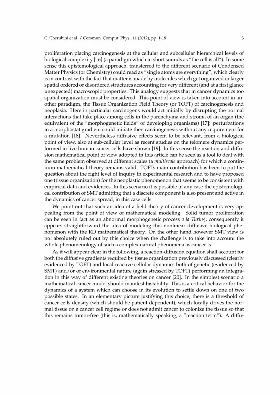
proliferation placing carcinogenesis at the cellular and subcellular hierarchical levels ofbiological complexity [16] (a paradigm which in short sounds as ”the cell is all”). In somesense this epistemological approach, transferred to the different scenario of CondensedMatter Physics (or Chemistry) could read as ”single atoms are everything”, which clearlyis in contrast with the fact that matter is made by molecules which get organized in largerspatial ordered or disordered structures accounting for very different (and at a first glanceunexpected) macroscopic properties. This analogy suggests that in cancer dynamics toospatial organization must be considered. This point of view is taken into account in an-other paradigm, the Tissue Organization Field Theory (or TOFT) of carcinogenesis andneoplasia. Here in particular carcinogens would act initially by disrupting the normalinteractions that take place among cells in the parenchyma and stroma of an organ (theequivalent of the ”morphogenetic fields” of developing organisms) [17]: perturbationsin a morphostat gradient could initiate then carcinogenesis without any requirement fora mutation [18]. Nevertheless diffusive effects seem to be relevant, from a biologicalpoint of view, also at sub-cellular level as recent studies on the telomere dynamics per-formed in live human cancer cells have shown [19]. In this sense the reaction and diffu-sion mathematical point of view adopted in this article can be seen as a tool to deal withthe same problem observed at different scales (a multiscale approach) for which a contin-uum mathematical theory remains valid. TOFTs main contribution has been to put thequestion about the right level of inquiry in experimental research and to have proposedone (tissue organization) for the neoplastic phenomenon that seems to be consistent withempirical data and evidences. In this scenario it is possible in any case the epistemologi-cal contribution of SMT admitting that a discrete component is also present and active inthe dynamics of cancer spread, in this case cells.

We point out that such an idea of a field theory of cancer development is very ap-pealing from the point of view of mathematical modeling. Solid tumor proliferationcan be seen in fact as an abnormal morphogenetic process a la Turing, consequently itappears straightforward the idea of modeling this nonlinear diffusive biological phe-nomenon with the RD mathematical theory. On the other hand however SMT view isnot absolutely ruled out by this choice when the challenge is to take into account thewhole phenomenology of such a complex natural phenomena as cancer is.

As it will appear clear in the following, a reaction-diffusion equation shall account forboth the diffusive gradients required by tissue organization previously discussed (clearlyevidenced by TOFT) and local reactive cellular dynamics both of genetic (evidenced bySMT) and/or of environmental nature (again stressed by TOFT) performing an integra-tion in this way of different existing theories on cancer [20]. In the simplest scenario amathematical cancer model should manifest bistability. This is a critical behavior for thedynamics of a system which can choose in its evolution to settle down on one of twopossible states. In an elementary picture justifying this choice, there is a threshold ofcancer cells density (which should be patient dependent), which locally drives the nor-mal tissue on a cancer cell regime or does not admit cancer to colonize the tissue so thatthis remains tumor-free (this is, mathematically speaking, a ”reaction term”). A diffu-


sive contribution makes cancer cells move around leading to a not only time but alsospace dependent problem. While continuum models (ordinary, partial or integro-partialdifferential equations or delay equations) can describe very well this cancer dynamics,also discrete models (cellular automata) seem to lead to positive results towards a possi-ble understanding of carcinogenesis [18]. This is not unexpected in fact because discretemodels (as cellular automata are) and continuum diffusion processes share many com-mon features in modeling nonlinear chemical and biological media [21, 22]: in particularcontinuum field theory can be seen as continuum limit of collective discrete behaviors.Mathematical modeling of bistability in cancer dynamics dates back to Lefever and Hors-themke work [23] although in the last thirty years many progresses have been done inthis area (see as an example [24] for a recent review on mathematical models). In exist-ing models bistability results as a consequence of complicated non-polynomial reactiveterms.

In this article instead we shall introduce and discuss a very basic model of reaction-diffusion bistability based on a cubic nonlinear diffusion equation only. This is inspiredby theoretical works calibrated on experimental data of brain tumor (see specifically [3,25–30]) through a single linear or nonlinear diffusion equation for cancer cells. Assuminga relatively simple mathematical form, these pre-existing studies have shown a great rele-vance for surgery due to the unpleasant and dramatic recurrences of brain tumors. Givena certain volume of brain tissue resection in fact, it is possible to predict the amount oftime required by the low density infiltrated tumor cells far afield from the gross tumorsite to cause a large cancer again. In this way the surgeon can perform a balanced pre-diction optimizing the amount of tissue removed in union with the quality of life left tothe patient. We shall frame our work on the lines of this type of studies then. To this aimhowever we shall need to introduce a short review of the mathematical aspects of RDprocesses first, as done in the next section.

2 Reaction-Diffusion systems

Reaction-Diffusion equations are mathematical models of parabolic type which describethe nonlinear concentration dynamics of one or more chemical substances. Differently asin standard global chemical kinetic problems, here the model allows the chemical speciesnot only to locally react but also to spatially diffuse one through the others. In a biologicalcontext instead RD systems describe fields of activators and inhibitors (in the languageintroduced by Alan Turing in [10]) which compete to give peculiar patterns (the animalcoat pattern theory) or even forms for the living beings (in Turing’s original article theproblem of gastrulation or of the form of an hydra). Here we present the prototype ofreaction-diffusion equations which assumes two variables only together with homoge-neous and isotropic diffusion. The equations in this case result in:

∂u

∂t= D1∇2u+ f (u,v),

∂v

∂t= D2∇2v+h(u,v), (2.1)


where f and h can have polynomial form in u and v, although more complicated func-tional dependencies (even on space and time) are allowed. Here D1 and D2 are thediffusion coefficients and ∇ is the gradient operator while ∇2 represents the Laplacianone. In general, models with two species only represent a simplification of more realis-tic situations in which several diffusing and reacting species can interact. Moreover bycoupling these models with temperature [31, 32] and mechanical deformations [33, 34]one can match even more the simulations with realistic biological problems. In the past,Turing showed that RD systems can be affected by the so called diffusion-driven insta-bility (or Turing instability) which means that if the homogeneous state is stable againstsmall perturbations in absence of diffusion, it may become unstable if the possibilityof diffusion is introduced. This dynamical mechanism generates quasi-stationary spa-tial patterns although this type of equations can also lead to morphogenetic, chemicalor electrophysiological waves [3]. Coming back to the model, an even simpler reaction-diffusion model can be obtained suppressing one of the two species in Eq. (2.1) (say fieldv) and assuming a simple cubic polynomial form for the function f (u) which could beseen as a Taylor expansion of more complicated functional dependencies, in analogy withFitzHugh-Nagumo type models of electrophysiology and physical chemistry [3, 35]: thisis the well-known bistable equation discussed in detail in the following.

3 A bistable model for cancer cell waves

The most generic one species reaction-diffusion equation is

∂tc= F(c)︸︷︷︸

Reaction

+∇·(

D∇c)

︸︷︷︸

Diffusion

, (3.1)

where we identify for our purposes the field c with the tumor cell punctual concentrationembedded in a pre-existing normal tissue and D is the diffusion tensor which in the mostgeneral scenario can depend by time and space (anisotropic and inhomogeneous diffu-sion). In this article however we shall assume for the sake of simplicity homogeneousand isotropic time independent diffusion first so that we can rewrite

∇·D∇c≡D∇2c,

where D is the diffusion constant. The term F(c) on the other hand takes into accountthe local dynamical properties of the system (reaction term) although one may extendthe treatment assuming F=F(c,t,~x), which gives heterogeneities of different physical na-ture (chemical, biological, physical). Finally one may could have easily added on thisreactive term of Eq. (3.1) an external time and space dependent stimulus which in ourspecific biological problem can account for possible external actions (chemotherapy as anexample). We have under-braced explicitly in Eq. (3.1) the reactive and diffusive termsrespectively. While the diffusive part can be seen as a typical TOFT quantity, the reactive


one, in the most general heterogeneous externally perturbed scenario, can contain both agenetically driven dynamics and an environmental factor: this modelization meets thenboth TOFT and SMT points of view about cancer origin. In mathematical terms, in ab-sence of diffusion we have a dynamical system with one degree of freedom (an OrdinaryDifferential Equation), while the introduction of diffusion leads immediately to an infi-nite degrees of freedom problem (this is a Partial Differential Equation problem in fact)where the nonlinear parabolic character of the problem accounts for spatial communica-tion and then possible global organization. We are ready now to specialize Eq. (3.1) to aparticular case, i.e., the bistable one, which requires for this equation a functional formF(c)= k(c−c1)(c−c2)(c3−c), where k is a model constant and c1, c2 and c3 are constantconcentrations which may be genetically determined but also environmentally affected.We assume that a cancer-free tissue must have no cancer cells so we select c1 =0. Quan-tity c2 instead represents the cancer generation threshold while c3 is the maximum valueof cancer cells which a tissue can support (possible necrosis effects lowering the tumorcell population are not taken into account here for the sake of simplicity). This equationmust be cast now in non-dimensional form: this step is crucial because removes from themodel the specifications of the particular tissue and cancer leading to a more general for-mulation. Following standard Literature [35], we introduce a typical length scale L of theprocess in consideration (working for the sake of simplicity in one spatial dimension first)and we define the non-dimensional quantities T= tD/L2 and X=x/L. We use moreoverthe scaling c2 =αc3 with 0<α<1, adopting a dimensionless concentration C = c/c3 thenand defining the quantity a= c2

3L2k/D. The resulting equation is:

∂C

∂T=

∂2C

∂X2+F(C), (3.2)

with the functional form

F(C)= aC(1−C)(C−α) (3.3)

with C = 0 and C = 1 being sinks and C = α being a source [36]. The process of adi-mensionalization performed has a great advantage that one can study now the dynamicsof the problem forgetting about the physical context we started from. The result ob-tained with the new compact equations can be later re-converted then to dimensionalquantities recovering the contact with experiments. This is a well known point of viewadopted both in chemistry and in electrophysiology. In the latter case, as an example, theFitzHugh-Nagumo equation (which is an extension in a two dimensional phase-space ofthe bistable equation just described), once solved in a specific dimensionless case can bedifferently framed in the context of heart, nerves or even intestine dynamics [35] throughspecific dimensional mappings of space, time and action potential. We point out that,all of these examples have different time, space and action potential scales. For this rea-son, in this article we shall present mainly the general outcomes expected studying thenon-dimensional theory, leaving to future studies the accurate analysis of mapping the


Figure 1: Bistable dynamics of the zero dimensional model with three different initial conditions: i) C0≡C(0)=0.11 (above the threshold α which implies cancer development); ii) C0 = 0.1 (on the threshold which impliesa (metastable) constant in time dynamics) and finally iii) C0 =0.09 (below the threshold which implies cancerrejection by tissue).

parameters with specific tumor growth processes and for different tissues. Higher dimen-sional spatial cases require the addition to this equation of the second derivative termswith respect to Y and Z. We point out that our treatment is quite different with respect tothe standard Verhulst logistic behavior commonly used to model cell growth [3,24,35,36]:here in fact we have a cubic behavior while in that case a quadratic one is adopted, miss-ing completely the threshold effect. Locally, i.e., neglecting the spatial variations, weobtain the ordinary differential equation dC/dT = F(C) which is, in the language of dy-namical systems, a flow on a line. Such a type of equation cannot have periodic solu-tions (unless the domain is topologically bent to form a circle [36]) and once integrated(we assume here and in the rest of the paper a = 1 and α = 0.1 which is a typical choicefound in the literature of bistable equation simulations [35] ) results in three type of pos-sible solutions shown in Fig. 1: i) a solution which starting over the threshold α reachesasymptotically the maximum value C = 1, ii) a solution starting on the threshold whichis stationary in time and iii) a solution starting below the threshold which asymptoticallygoes to zero.

Reintroducing diffusion we have a partial differential equation which as discussedbefore, has infinite degrees of freedom and can lead in fact to more involved situationsin which diffusion plays a central role. Manipulations of the one-dimensional diffusingcase in Eq. (3.2) lead to the analytical travelling wave solution for the bistable equationassociated with specific initial data and boundary conditions (well known in the litera-ture) [35]

C(T,X)=1

2+

1

2tanh

[√a(X+VT)

2√

2

]

, V =

√a√2(1−2α). (3.4)

It is clear the wave type behavior of this solution which travels at constant speed (de-


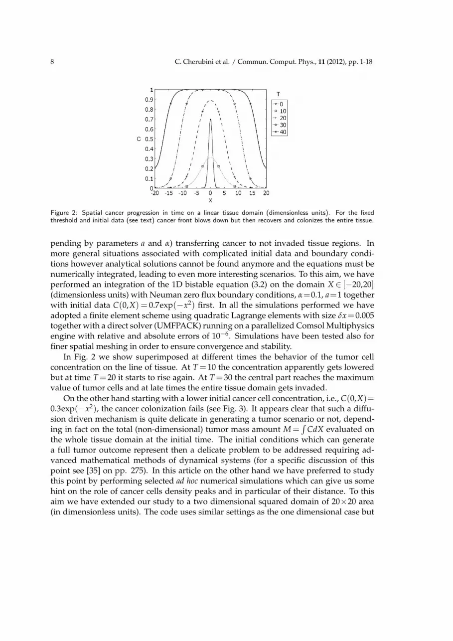
Figure 2: Spatial cancer progression in time on a linear tissue domain (dimensionless units). For the fixedthreshold and initial data (see text) cancer front blows down but then recovers and colonizes the entire tissue.

pending by parameters a and α) transferring cancer to not invaded tissue regions. Inmore general situations associated with complicated initial data and boundary condi-tions however analytical solutions cannot be found anymore and the equations must benumerically integrated, leading to even more interesting scenarios. To this aim, we haveperformed an integration of the 1D bistable equation (3.2) on the domain X ∈ [−20,20](dimensionless units) with Neuman zero flux boundary conditions, α=0.1, a=1 togetherwith initial data C(0,X) = 0.7exp(−x2) first. In all the simulations performed we haveadopted a finite element scheme using quadratic Lagrange elements with size δx=0.005together with a direct solver (UMFPACK) running on a parallelized Comsol Multiphysicsengine with relative and absolute errors of 10−6. Simulations have been tested also forfiner spatial meshing in order to ensure convergence and stability.

In Fig. 2 we show superimposed at different times the behavior of the tumor cellconcentration on the line of tissue. At T = 10 the concentration apparently gets loweredbut at time T =20 it starts to rise again. At T =30 the central part reaches the maximumvalue of tumor cells and at late times the entire tissue domain gets invaded.

On the other hand starting with a lower initial cancer cell concentration, i.e., C(0,X)=0.3exp(−x2), the cancer colonization fails (see Fig. 3). It appears clear that such a diffu-sion driven mechanism is quite delicate in generating a tumor scenario or not, depend-ing in fact on the total (non-dimensional) tumor mass amount M =

∫CdX evaluated on

the whole tissue domain at the initial time. The initial conditions which can generatea full tumor outcome represent then a delicate problem to be addressed requiring ad-vanced mathematical methods of dynamical systems (for a specific discussion of thispoint see [35] on pp. 275). In this article on the other hand we have preferred to studythis point by performing selected ad hoc numerical simulations which can give us somehint on the role of cancer cells density peaks and in particular of their distance. To thisaim we have extended our study to a two dimensional squared domain of 20×20 area(in dimensionless units). The code uses similar settings as the one dimensional case but


Figure 3: Spatial cancer no-progression in time on a linear tissue domain (dimensionless units). For the fixedthreshold and initial data (see text) cancer front blows down and tissue remains cancer cell free.

regarding the meshing we have adopted squared sized (side length δx =0.25) Lagrangecubic elements.

Results of the simulations are shown in Fig. 4. We have taken an initial data addingseveral distorted Gaussian functions centered at different points. In this approach, for afixed choice of model constants α and a, there are clearly three critical parameters whichcan affect the entire dynamics: the Gaussian peak amplitudes, their widths and finallytheir distance. In our case we have chosen specifically:

C0 =0.8e−0.1(x−1)2−0.3(y−3)2+0.75e−0.25(x−10)2−0.15(y+9)2

+0.6e−0.2(x+3)2−0.5(y+4)2+0.5e−0.25(x+5)2−0.3(y−1)2

(3.5)

and left it free to evolve. The remaining panels of Fig. 4 show the cancer spread andfinally a large scale invasion dynamics. We have performed also a more simplified studyin order to understand if two over-threshold cell colonies of Gaussian form may lead to atumor progression or extinction scenario depending on the distances of their peaks only.To this aim we have taken as initial data

C0 =0.61e−0.1(x−4)2−0.3y2+0.61e−0.1(x+4)2−0.3y2

, (3.6)

which has lead to a final tumor progression as shown in Fig. 5.On the other hand the initial data

C0 =0.61e−0.1(x−6)2−0.3y2+0.61e−0.1(x+6)2−0.3y2

(3.7)

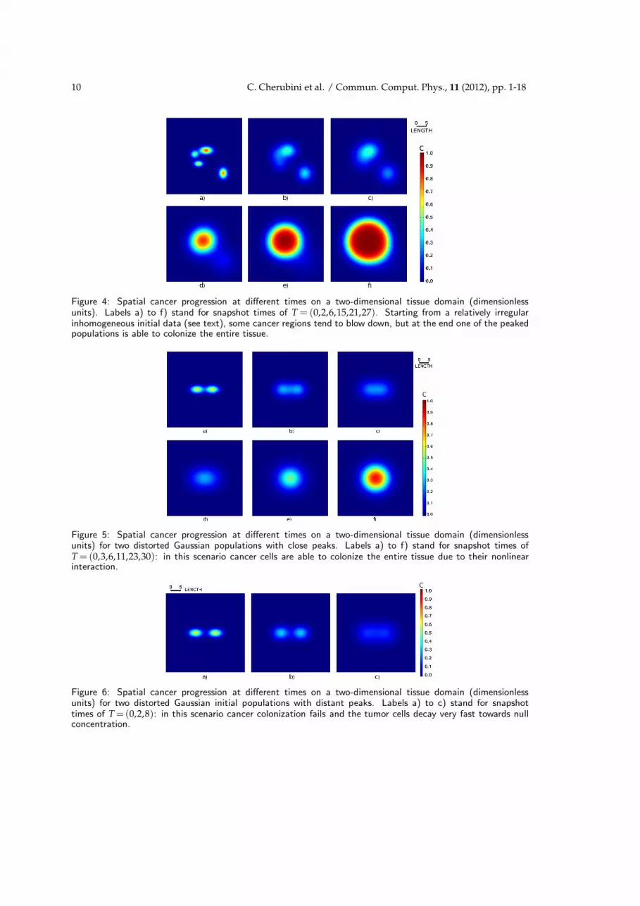
has not given any tumor progression as shown in Fig. 6. These results suggest that thenonlinear interaction of the two waves leads to a critical configuration which has canceras an outcome, while if the two distorted Gaussian colonies are slightly more distant,the nonlinear mechanism is not sufficient to maintain the developmental process and the


Figure 4: Spatial cancer progression at different times on a two-dimensional tissue domain (dimensionlessunits). Labels a) to f) stand for snapshot times of T = (0,2,6,15,21,27). Starting from a relatively irregularinhomogeneous initial data (see text), some cancer regions tend to blow down, but at the end one of the peakedpopulations is able to colonize the entire tissue.

Figure 5: Spatial cancer progression at different times on a two-dimensional tissue domain (dimensionlessunits) for two distorted Gaussian populations with close peaks. Labels a) to f) stand for snapshot times ofT = (0,3,6,11,23,30): in this scenario cancer cells are able to colonize the entire tissue due to their nonlinearinteraction.

Figure 6: Spatial cancer progression at different times on a two-dimensional tissue domain (dimensionlessunits) for two distorted Gaussian initial populations with distant peaks. Labels a) to c) stand for snapshottimes of T =(0,2,8): in this scenario cancer colonization fails and the tumor cells decay very fast towards nullconcentration.


total cancer cells density vanishes in time. This model generalized in three dimensions(blocks of tissue) has to be calibrated on experiments, in order to estimate a realistic initialdata, the diffusion coefficient and the physiological threshold α which could be patientdependent and possibly genetically and/or environmentally ruled [37].

Clearly stochastically induced mutations as well as instabilities driven by diffusion,angiogenesis and so on must play an important role in cancer development (see [24] andthe more recent [38] for a discussion on the role of field theories in carcinogenesis). On theother hand, as anticipated already, an active field of research in tumor modeling adopts asingle reaction-diffusion equation (see [3,25–30] for details) to model solid cancer growthin anatomically correct 3D brain geometry (as already analyzed in [39] by some of theauthors).

4 Bistable dynamics with ecological dispersal effects

We can now extend in a novel way the theory previously introduced, borrowing fromthe ecological models the possibility to have population dispersal. Discrete models [40]have been proposed to reproduce these properties. In this work we propose a continuumapproach instead. The starting point of such a formulation is the experimental evidencethat populations of animals in a territory diffuse with a certain (mean) speed dependingby the density of animals in that region. Stated in a more straight way, if there are toomany individuals in certain region, they tend to exhaust rapidly the local food suppliesso that they should abandon the area as soon as possible. If their concentration is not sohigh on the other hand, they could spread around more slowly. Clearly such a point ofview should work correctly also for bacteria, viruses and other microorganisms as well asfor solid cancer cells, which in this simplified scenario would migrate because of the eco-logical pressure. Clearly this is a very basic starting point for more refined modelizationswhich should take into account also the role of chemotaxis and angiogenesis [3] togetherwith advective effects for oxygen and nutrients and the importance of the immune sys-tem in these matters. Anyway this simplified point of view makes the formulation non-trivial because it requires mathematically to have a diffusion coefficient which dependsby the local concentration of the diffusing field, i.e., in our case D = D(c). Borrowingagain from ecological models the theoretical formulation, we assume the isotropic powerlaw functional dependence D=D ·

[c(t,~x)/cre f

]mI, where D is the diffusion constant, cre f

is a reference constant concentration, here introduced for dimensional analysis reasons,m is a non negative real number and I is the identity matrix. Rewriting cre f = σc3 withσ>0, and adopting the same non-dimensional quantities previously discussed, we finallyarrive to the dimensionless equation

∂C

∂T=σ−m∇·

(Cm∇C

)+F(C), (4.1)

which in the limit m→0 reduces to the standard bistable equation previously discussed(in 1D Eq. (3.2)) while if F(C) = 0, becomes the porous media equation which has an-


alytical solutions in one dimensions [3]. Eq. (4.1) in 1D can be studied with the usualprocedure adopted to find travelling wave solutions. Requiring C = C(X+VT)≡C(ξ)(here V is the constant velocity of the pulse), it becomes

σ−m d

dξ

(

Cm d

dξC

)

−VdC

dξ+F(C)=0, (4.2)

which could be possibly studied in search of analytical solutions or numerically as aboundary value problem for the allowed values of the constant V, again. Although thiswould lead to an interesting mathematical problem, from the physical point of view, suchtravelling waves of constant velocity V should be regarded in the best case as asymp-totic states in time of more complicated solutions which already in the 1D case do nottravel always at constant speed. The reason for this is that the dimensionless velocityof the standard bistable pulse in Eq. (3.4), once rewritten in dimensional variables, givesa velocity which grows linearly with the (constant) diffusion coefficient. The additionof dispersal implies a non constant diffusion coefficient (monotonically increasing withfield concentration) so that, if one assumes a very slow growth of the density, the speedof the pulse too should change analogously and a constant speed travelling wave wouldnot be possible. However, once the system reaches its highest asymptotic concentrationvalue due to the bistable dynamics, practically a constant diffusion coefficient occurs sothat constant speed travelling wave appears. In order to prove this scenario and havea complete view of the real dynamics of this extended model, we have studied Eq. (4.1)adopting the same codes for the numerical simulation previously discussed in the simplebistable case, requiring for the sake of simplicity σ = 1 and m = 1 (a linear growth fordiffusion in function of concentration which is in agreement with the literature [3]).

In Fig. 7 (to be compared with Fig. 2) we show the evolution of the tumor at differ-ent times with initial data C(0,x)=0.7exp(−x2) again. Notice the sharp interface of thecell front with the zero tumor region, which is totally absent in the simple diffusive case.The inclusion of the porous medium term in fact leads to a quasilinear partial differen-tial equation, eliminating the unpleasant regularizing effect of the heat operator whichgenerates a nonzero concentration in the entire domain (infinite propagation velocity).

In Fig. 8 (to be compared with Fig. 3) we can see that, differently than in the diffusivecase, the smaller initial data C(0,x) = 0.3exp(−x2) leads in any case to tumor cell pro-gression which has a different propagation velocity in time. In fact by focusing on theX-axis, one can see that at equidistant time intervals, the interface covers different spacesmanifesting the expected concentration-dependent velocity of propagation which, oncethe upper concentration limit is reached, becomes approximately constant, confirmingthe physical scenario previously hypothesized.

A space-time diagram of the latter simulation shows this effect quantitatively as shownin Fig. 9 where there is a strong change in the slope (so in speed) due to the change of con-centration. In Fig. 10 we present instead the space-time diagram for the interaction of thetwo initial data just discussed by assuming C(0,X)=0.7exp(−(x−10)2)+0.3exp(−(x+10)2). We point out the change in slopes of the smaller distorted Gaussian in comparison


Figure 7: Spatial cancer progression in time on a linear tissue domain (dimensionless units) in the case ofpopulation dispersal for initial data C(0,x)=0.7exp(−x2).

Figure 8: Spatial cancer progression in time on a linear tissue domain (dimensionless units) in the case of

population dispersal for initial data C(0,x) = 0.3exp(−x2). Differently as in the simpler reaction-diffusiontheory, here even smaller initial data can lead to tumor progression.

with the higher one and the nonlinear interaction on the collision area.We can now analyze the dynamics in higher dimensional cases. In three dimensions,

assuming a purely radial dynamics, one starts from cartesian coordinates, adopts thesame non-dimensional notations as in the one-dimensional case, and passing to dimen-sionless spherical coordinates (R,θ,φ), finally obtains:

∂C

∂T=

σ−m

R2

d

dR

(

CmR2 d

dRC

)

+F(C). (4.3)

This spherical scheme shall have relevance for realistic NMR imported 3D brain geome-tries, on the lines of precedent studies of some of the authors [39], performing a fine


Figure 9: Space-time diagram of cancer progression in time on a linear tissue domain (dimensionless units) in

the case of population dispersal for initial data C(0,x)= 0.3exp(−x2). Notice the change of slope meaning achange of tumor progression speed.

Figure 10: Space-time diagram of cancer interaction for the initial data C(0,X) = 0.7exp(−(x−10)2)+0.3exp(−(x+10)2). Due to the dispersal term the various populations interact nonlinearly with differentspeeds.

Figure 11: Space-time development of cancer growth in the cylindrical (planar radial) self-diffusing case for

initial data C(0,ρ)=0.3e−0.1ρ2.

tuning of the model parameters with radiological data taken at different times. Anotherpossible field of application of this modelization is in the context of cancerous cell cul-tures. In circular dimensionless cylindrical coordinates (ρ,φ,Z), assuming purely radial


Figure 12: Mean value of tumor radius versus time in the case of Fig. 11.

diffusion (typical of cell cultures situations which are almost planar) we obtain instead

∂C

∂T=

σ−m

ρ

d

dρ

(

Cmρd

dρC

)

+F(C). (4.4)

Taking as initial data C(0,ρ)=0.3e−0.1ρ2and zero flux again as boundary conditions [41],

we obtain the spacetime diagram in Fig. 11.In Fig. 12 we have plotted instead the mean radial distance of the cancer population

from the origin versus time (see [3] pp. 553 for this definition), i.e.,

〈ρ〉=∫ ρo

0 ρ2C(ρ,T)dρ∫ ρo

0ρC(ρ,T)dρ

, (4.5)

where ρo represent the outer boundary of the Petri dish which in our case has valuetwenty space dimensionless units. On page 555 of [3], based on experimental resultsby [42], an estimate, in vitro, of an (approximate) value of the mean radius versus timefor an anaplastic astrocytoma, a mixed glioma and a glioblastoma multiforme culturesgrowing can be found. More in detail it is approximated by

〈ρ〉≃∫ ρo

λ ρ(ρ−λ)C(ρ,T)dρ∫ ρo

λ ρC(ρ,T)dρ, (4.6)

where λ2 represents the uniform steady state of the cell distribution. Scaling the variablesit is possible to obtain a growing trend for the tumor mean radius in qualitative agree-ment with some of these experiments, in particular in the case of the mixed glioma. Thetwo other types of tumors on the other hand manifest a different regime so our modelshould be fine tuned also in the functional form of D(c) in order to fit these data. A setof parametric simulations in which (m,σ,a,α) are varied shall improve the agreement ofthe model with experiments, especially for values of m close to zero (i.e., standard diffu-sion). We plan to perform all of these works in future studies in union with additionalexperimental data [37].


5 Conclusions

In this article we have introduced and discussed a very basic model of cancer spreadwhich grasps the main feature of solid cancer progression in tissues, i.e., the possibilityfor the tumoral cell colonization to occur or the blocking action of this process due todifferent biological reactions of the organism. The model is based on the bistable equa-tion, which can be seen as a polynomial approximation [36] for many different morecomplicated biological scenarios making the formulation very general. The inclusion ofdispersal effects makes the formulation absolutely nontrivial but much more interestingbecause of the possibility to have different propagation speed in association with differ-ent cancer cells densities in the tissue. It is important to remark also that this modelizationcould play a central role not only in the field of cell growth modeling but also in the fieldof computational electrophysiology where reaction-diffusion theory with simple diffu-sion (and not with porous medium term) is commonly adopted to study electrochemicalwaves in biological media.

This article is a starting point for a field theoretical approach of cancer progressionformulated in terms of very basic but at the same time very general equations aimingto extend in future the successful experimental and theoretical works regarding braincancer [3, 25–30] with the techniques on real brain geometries developed by some of theauthors in the past. The hope is to find, through mathematical modeling, some gen-eral behaviors which could be extrapolated from the patient dependent specific scenario,in analogy with other branches of Theoretical Physics in which apparently different sys-tems simplify towards a common description once well expressed in mathematical terms.Such a formalization of cancer spread can bridge the requirements of the major exist-ing interpretative theories. Nevertheless, any methodological approach needs a greaterawareness of the complexity of the organism, which appears nowadays more and moreevident, in order to develop consistent mathematical tools for modeling.

Acknowledgments

Two of the authors (C. Cherubini and S. Filippi) acknowledge ICRANet for partial finan-cial support.

References

[1] W. T. D’Arcy, On Growth and Form, Cambridge University Press, 1992.[2] D. Bini, C. Cherubini, S. Filippi, A. Gizzi and P. E. Ricci, On spiral waves arising in natural

systems, Commun. Comput. Phys., 8 (2010), 610–622.[3] J. D. Murray, Mathematical Biology, 3rd edition in 2 volumes, Springer, 2004.[4] A. T. Winfree, The Geometry of Biological Time, 2nd edition, Springer, 2001.[5] A. T. Winfree, When Time Breaks Down: The Three-Dimensional Dynamics of Electrochem-

ical Waves and Cardiac Arrhythmias, Princeton University Press, 1987.


[6] R. V. Jean, Phyllotaxis: A Systemic Study in Plant Morphogenesis, Cambridge UniversityPress, 1994.

[7] Y. Kuramoto, Chemical Oscillations, Waves and Turbulence, Dover, 2003.[8] D. Kondepudi and I. Prigogine, Modern Thermodynamics: From Heat Engines to Dissipa-

tive Structures, Wiley, 1998.[9] I. R. Epstein and J. A. Pojman, An Introduction to Nonlinear Chemical Dynamics, Oxford

University Press, 1998.[10] A. M. Turing, The chemical basis of morphogenesis, Phil. Trans. Roy. Soc. B, 237 (1952), 37–

72.[11] C. Panetta, M. A. J. Chaplain and J. Adam, The mathematical modelling of cancer: a re-

view, Proceedings of the MMMHS Conference (eds. M. A. Horn, G. Simonett and G. Webb),Vanderbilt University Press, 1998.

[12] E. R. Fearon and B. Vogelstein, A genetic model for colorectal tumorigenesis, Cell, 61 (1990),759–767.

[13] A. M. Soto and C. Sonnenschein, The somatic mutation theory of cancer: growing problemswith the paradigm, BioEssays, 26 (2004), 1097–1107.

[14] C. Sonnenschein and A. M. Soto AM, Theories of carcinogenesis: an emerging perspective,Semin. Cancer Biol., 18 (2008), 372–377.

[15] J. D. Potter, Morphostats, morphogens, microarchitecture and malignancy, Nat. Rev. Cancer,7 (2007), 464–474.

[16] R. A. Weinberg, One Renegade Cell: How Cancer Begins, New York, Basic Books, 1998.[17] C. Sonnenschein and A. M. Soto, Somatic mutation theory of carcinogenesis: why it should

be dropped and replaced, Mol. Carcinog., 29 (2000), 205–211.[18] S. G. Baker, A. M. Soto, C. Sonnenschein, A. Cappuccio, J. D. Potter and B. S. Kramer, Plau-

sibility of stromal initiation of epithelial cancers without a mutation in the epithelium: acomputer simulation of morphostats, BMC Cancer, 9 (2009), 89.

[19] X. Wang, Z. Kam, P. M. Carlton, L. Xu, J. W. Sedat and E. H. Blackburn, Rapid telomeremotions in live human cells analyzed by highly time-resolved microscopy, Epigenetics &Chromatin, 1 (2008), 4.

[20] M. Bertolaso, Towards and integrated view of the neoplastic phenomena in cancer research,Hist. Phil. Life Sci., 31 (2009), 79–98.

[21] S. Wolfram, A New Kind of Science, Wolfram Media, 1st edition, 2002.[22] B. Chopard and M. Droz, Cellular Automata Modeling of Physical Systems, Cambridge

University Press, 1998.[23] R. Lefever and W. Horsthemke, Bistability in fluctuating envitonments, implications in tu-

mor immunology, Bull. Math. Biol., 41 (1979), 269–290.[24] D. Wodarz and N. L. Komarova, Computational Biology of Cancer: Lecture Notes and Math-

ematical Modeling, World Scientific, 2005.[25] K. R. Swanson, E. C. Alvord and J. D. Murray, A quantitative model for differential motility

of gliomas in grey and white matter, Cell Proliferation, 33(5) (2000), 317–330.[26] K. R. Swanson, E. C. Alvord Jr and J. D. Murray, Quantifying efficacy of chemotherapy of

brain tumors (gliomas) with homogeneous and heterogeneous drug delivery, Acta Biotheo-retica, 50(4) (2002), 223–237.

[27] K. R. Swanson, E. C. Alvord Jr. and J. D. Murray, Virtual resection of gliomas: effects oflocation and extent of resection on recurrence, Math. Comput. Model., 37 (2003), 1177–1190.

[28] K. R. Swanson, C. Bridge, J. D. Murray and E. C. Alvord Jr, Virtual and real brain tumors:using mathematical modeling to quantify glioma growth and invasion, J. Neurological Sci.,


216(1) (2003), 1–10.[29] K. R. Swanson, E. C. Alvord, Jr. and J. D. Murray, Dynamics of a model fro brain tumors

reveals a small window for therapeutic intervention, Disc. Cont. Dyn. Syst. B, 4(1) (2004),289–295.

[30] H. L. P. Harpold, E. C. Alvord Jr. and K. R. Swanson, Visualizing beyond the tip of theiceberg: the evolution of mathematical modeling of glioma growth and invasion, J. Neu-ropathol. Exp. Neurol., 66 (2007), 1–9.

[31] D. Bini, C. Cherubini and S. Filippi, Heat transfer in FitzHugh-Nagumo model, Phys. Rev.E, 74 (2006), 041905.

[32] C. Cherubini, S. Filippi, P. Nardinocchi and L. Teresi, An electromechanical model of car-diac tissue: constitutive issues and electrophysiological effects, Prog. Biophys. Mol. Biol., 97(2008), 562–573.

[33] D. Bini, C. Cherubini and S. Filippi, Viscoelastic FitzHugh-Nagumo models, Phys. Rev. E, 72(2005), 041929.

[34] D. Bini, C. Cherubini and S. Filippi, On vortices heating biological excitable media, Chaos,Solitons & Fractals, 42 (2009), 2057–2066.

[35] J. Keener and J. Sneyd, Mathematical Physiology, Springer, 2001.[36] S. H. Strogatz, Nonlinear Dynamics and Chaos: with Applications to Physics, Biology,

Chemistry and Engineering, Westview Press, 2001.[37] C. Cherubini, A. Gizzi, M. Bertolaso, V. Tambone and S. Filippi, in preparation, 2010.[38] S. G. Baker, A. Cappuccio and J. D. Potter, Research on early-stage carcinogenesis: are we

approaching paradigm instability?, J. Clin. Oncol., 28 (2010), 3215–3218.[39] C. Cherubini, S. Filippi and A. Gizzi, Diffusion processes in human brain using COMSOL

multiphysics, Proceedings of COMSOL Users Conference of Milan, Italy, 2006.[40] D. E. Marco, S. A. Cannas, M. A. Montemurro, B. Hu and S. Y. Cheng, Comparable ecological

dynamics underlie early cancer invasion and species dispersal, involving self-organizingprocesses, J. Theor. Biol., 256 (2009), 65–75.

[41] K. W. Morton and D. F. Mayers, Numerical Solutions of Partial Differential Equations, Cam-bridge University Press, 1994.

[42] M. R. Chicoine and D. L. Silbergeld, Assessment of brain tumor cell motility in vitro and invivo, J. Neurosurg., 82 (1995), 615–622.

a bistable field model of cancer dynamics

Documents