Statics and Dynamics of a Nanowire in Field Emission

A. Lazarus∗,a, E. de Langrea, P. Mannevillea,P. Vincentb, S. Perisanub, A. Ayarib, S. Purcellb

aLaboratoire d’Hydrodynamique, Ecole Polytechnique, 91128 Palaiseau, FrancebLaboratoire PMCN, CNRS Universite Lyon 1, 69622 Villeurbanne, France

Abstract

We simulate the nonlinear behaviour of a cantilevered nanowire in field emis-sion to understand and exploit the self-oscillations experimentally observedin this NanoElectroMechanical System. The original coupling taking placein this oscillator is predicted with a low-dimensional model consisting of abi-articulated cantilevered beam flowing electrons and immersed in an elec-trostatic environment. We propose a simple model to set up the qualitativenonlinear governing equations of the system and also highlight the elaborateequilibrium between the electrostatic field, the nanowire motion and the elec-tric field emission current. A linear stability analysis of the nonlinear staticfixed points aims at determining the instability threshold as a function of theapplied DC voltage. It is found that instability is mostly due to the competi-tion between the field emission current dependence on the nanowire positionand the voltage. As a consequence, the emergence of flutter requires specificexternal conditions such as an initial angular imperfection, a strong mechani-cal Q factor or a high electrical resistance. Finally, a direct integration of thenonlinear governing equations confirms the presence of high-frequency self-oscillations, i.e. the possibility of DC/AC conversion in this autonomouselectromechanical device.

Key words: Nanotechnology, electro-mechanical coupling, slenderstructures dynamics, linear stability

∗Corresponding authorEmail addresses: lazarus@ladhyx.polytechnique.fr (A. Lazarus),

delangre@ladhyx.polytechnique.fr (E. de Langre)

Preprint submitted to International Journal of Mechanical Science September 1, 2009

Nomenclature

Kinematics

D Diameter of the nanowireL Length of the nanowireq1, q2 Absolute angular displacementsθ1, θ2 Angular displacements around the tilting positionψ Initial angular tilting of the nanowire

Electrostatics

C, c Electrical capacitance and its dimensionless formCref Electrical capacitance when q1 = q2 = 0E, e Electric field and its dimensionless formF Electrostatic force applied on the nanowireM1A, M2A, M2B Moments of the electrostatic forces about the two artic-

ulations A and Bm1A, m2A, m2B Dimensionless forms of the electrostatic momentsU, u Electric potential and its dimensionless formS Boundary of the electrostatic problemβ, b Field enhancement factor and its dimensionless formβref Field enhancement factor when q1 = q2 = 0

Mechanics

ak Rotational stiffness ratio of the interconnected springsµ Viscous damping of the interconnected damperskA, kB Rotational stiffnesses of the interconnected springsm Nanowire mass per unit lengthQ Dimensionless mechanical quality factorτ Dimensionless time scaleϕ

1, ϕ

2Shapes of the first and second mechanical mode

ω Reference frequency of the oscillating nanowire

2

Electricity

Ic Capacitor currentIe, ie Field emission current and its dimensionless formH, G, h, g Fowler-Nordheim empirical constants and dimensionless

formsR Nanowire electrical resistancer Ratio between electrical and mechanical time scalesU , u Voltage at the nanowire tip and its dimensionless formV , v Applied DC voltage and its dimensionless formUref Field emission voltage referenceϕ

3Electrical mode shape

1. Introduction

Nanoelectromechanical Systems (NEMS) based on mechanical resonancesof nanostructures, such as nanotubes or nanowires, are drawing interest fromboth technical and scientific communities [1]. Their extremely small dimen-sions make them highly sensitive to external electrostatic perturbations and,due to their outstanding mechanical properties such as strong Young mod-ulus or high quality factor Q, [2], their mechanical response can exceed thequality of electrical signals from purely electronic devices. As well, NEMSoscillators have been proposed for use in ultrasensible mass detection [3] orradio frequency for wireless communication [4].

Among the great variety of these nanocomponents, NEMS based on singlyclamped cantilevers in field emission (FE) configuration have recently provenoriginal capabilities [5]. In this FE configuration, a nanotube or nanowireis connected to the cathode and a DC voltage V is applied between thecathode and an anode positioned in the vicinity of the nanostructure (Figure1). For a voltage Uref , the electric field at the nanowire apex, enhanced byits tip effect, becomes sufficient to extract electrons by tunneling effect. Thisquantum process results in a field emission DC current depending on theapplied voltage V , [6].

One of the originality when using cantilevered nanostructures as fieldemitters is that their extreme mechanical sensitivity reveals dependence ofthe FE current on the position of the emitter. The new NEMS applicationsin this configuration take advantage of this original coupling between theemitted current and the position of the emitter apex in its environment.One can also mention that this configuration is well adapted for mechanical

3

studies on nanotubes and nanowires, as the resulting patterns of the emittedelectrons give a direct projection of the apex motion on a phosphor screen(Figure 1). This allows investigations of linear and nonlinear behaviour ofnanocantilevers [7, 8].

Figure 1: Experimental settings : nanowire in field emission

A particularly interesting application recently shown by Ayari et al. [9],using highly resistive nanowires, has been the observation of self-oscillationsresulting from the electromechanical interactions between the electrical andmechanical properties of the cantilever. They showed that above a crit-ical DC voltage, the nanostructure starts to oscillate resulting in an ACfield emission current. The realization of an AC current generator at thenanoscale simply commanded by a DC voltage has interesting potentialitiesin autonomous nanosystems such as smart dust applications. From a theoret-ical point of view, this system exemplifies an original coupling that appearsat the nanoscale between mechanical behaviour, electrostatic environmentand FE properties.

The present paper proposes nonlinear simulations to predict nonlinearstatics and dynamics of a nanowire in field emission. Inspired by the fluid-structure interaction formalism for modelling the instability of slender struc-tures in axial flow [10, 11], we describe a discrete model to understand and

4

also make the most of the physical phenomena involved in this original na-noelectromechanical system. Based on the first investigations by Ayari etal. [9], we extend their model to a rigorous geometrically nonlinear one withricher kinematics. The electrostatic problem, the mechanical behaviour andthe field emission influence are successively discussed. This work provides afirst qualitative model of a cantilevered nanowire in field emission but canalso be extended to the modelling of vibrating nanostructures so far mainlybased on linear beam theory [12].

In Section 2, we set up the general governing equations of a bi-articulatednanowire in field emission, which is expected to be a suitable low-dimensionalmodel to compute qualitative results. The electrostatic environment of thenanostructure governs the applied electrostatic forces and some essential elec-trical properties respectively required to set up the coupled mechanical andelectrical models. The complete dimensionless nonlinear formulation of thediscrete system is given at the end of the section. We then specify theparameters of the model related to the physical problem for further compu-tations. The chosen kinematics leading to a low-dimensional governing equa-tion, many discrete electromechanical parameters are determined through ex-perimental observations of the continuous system. The remaining unknownquantities are obtained by computing the electrostatic problem. In Section 4,we perform the numerical simulation of a nanowire in field emission. We con-firm the possibility of self-oscillations around the system static equilibrium.An explanation of the physical phenomenon responsible for the instabilityis suggested in appendix. A parametric study of the NEMS linear stabilityallows us determining the electrical and mechanical parameters leading toself-oscillations. Finally, implicit time integration is performed to simulatethe limit cycles and the output AC signal of the nanodevice at the instabilitythreshold.

2. Fully nonlinear model of a nanowire in field emission

In order to set up the governing equations of the nanowire in field emis-sion, one needs first to sort out the strong connections between the differentphysical problems contained in the system, i.e. the electrostatic, the mechan-ical and the electrical ones. In the following, after choosing an appropriatekinematics, we show how to compute the electrostatic problem giving us therequired variables to study further the dynamics of our nanoemitter. Indeed,once this done, the nanowire motion and its electrical equilibrium are com-

5

pletely defined at any instant t and the dimensionless governing equations ofthe electromechanical system can then be given.

2.1. Kinematics

The diagram in Figure 2.a illustrates the kinematics chosen to model thedynamical behaviour of a cantilevered nanowire with length L and diameterD in the field emission setup presented in Figure 1. The geometrical con-figuration of the oscillating nanowire is described at any instant t by twogeneralised coordinates q1 and q2 such that

q1 (t) = θ1 (t) + ψ,

q2 (t) = θ2 (t) + ψ(1)

where the constant ψ is the initial angle made by the nanowire with thez axis considered as the symmetrical FE configuration. Indeed, nanowiresbeing electrostatically glued on the tungsten tip, their initial positions aregenerally not symmetrical [7].

(a) Kinematics of the nanowire (b) Sketch of the electrostatic problem

Figure 2: Cantilevered bi-articulated nanowire immersed in electrostatic field

Note that simulations of articulated models have been widely used as an aidin the study of their continuous flexible counterparts in the field of dynam-ics [10]. In accordance with the physical problem and the purpose of thepaper, this two degrees-of-freedom model is expected to be sufficient to cap-ture the essential dynamical features of the continuous system (geometrical

6

nonlinearities, instability mechanism, self-oscillations). Furthermore, sincemost of the methods for analysing nonlinear systems are practicable onlyfor low-dimensional systems, we follow the tendency to study a simplifieddiscretization of the continuous system.

2.2. Electrostatic Model

In the field emission configuration (Figure 1), the applied DC voltage Vleads to an electrical potential difference U between the nanowire and theUltra High Vacuum environment. Thereby, external electrostatic forces willact on the two segments of our bi-articulated nanostructure which behaves asone armature of a capacitor. According to the FE configuration (dimensionsinvolved, Ultra High Vacuum chamber experiments), we consider that elec-trostatic interactions are an order of magnitude larger than other physicalphenomenon such as gravitational or Van der Waals forces, or Casimir andthermal effects. Electrostatic considerations are accordingly the only onestaken in account.The electrostatic problem consists in the determination of the electric poten-tial field U in the vacuum domain under boundary conditions [13]. Under theassumptions of static potentials and no electrical charges inside the domain[14], this electrostatic problem can be reduced to the Laplace equation

∆U = 0. (2)

The unique solution of the Laplace’s equation must satisfy the Dirichletboundary conditions imposed by the physical situation sketched in the Figure2.b: A constant potential U0 is imposed on the base S0, the metallic structurecomposed of the tungsten tip support and the nanowire. The top surface S1

is raised to a potential U1 in order to simulate the voltage U = U1 − U0

between the nanowire apex and its environment. Finally, we impose a lin-ear evolution between U0 and U1 on the lateral face S2. Boundaries S1 andS2 are choosen far enough from the nanowire to fulfil the hypothesis of asemi-infinite dielectric medium.Once the electric potential U is defined in the whole domain, the electric fieldis easily deduced [13] according to

E = −∇U. (3)

Under the classical requirement that the electric field be everywhere per-pendicular to the surface of the conductor, the electrostatic forces can be

7

computed from the field at the surface of the nanowire following

F =1

2ǫ0SE. (E, n) (4)

where ǫ0 = 8.85×10−12 F/m is the permittivity of vacuum and n is the outernormal vector of the nanowire surface S. From an electrical point of view,the capacity between the nanowire and its environment derives simply [13]from the electric field E following

C =

∫

S2ǫ0E.ndS

U1 − U0

. (5)

A last electrical variable provided by the electrostatic problem is the fieldenhancement factor β illustrating the nanowire tip effect and involved in theexpression of the FE current. Here, β is the ratio between the electric fieldmagnitude at the emitter apex and the electrical potential difference U andreads

β =E (W ) .n

U1 − U0

(6)

where W is the point at the nanowire very end considered to be the emissionsurface (Figure 2.b). The boundary value problem (2) is related to the geo-metrical configuration of the frontier S0. According to the chosen kinematics,all the electrostatic quantities depicted in this part depend on the nanowiremotion, characterized by the generalised coordinates q1 and q2. Moreoverthe electrostatic forces F depend on potential difference U and may alsobe written as F (q1, q2, U). The electrical quantities C and β actually donot dependent on U since they are expressed in the form −∇U/U and readC (q1, q2) and β (q1, q2).

2.3. Mechanical Model

We may now introduce the equations governing the motion of the cantileverednanowire in field emission. The diagram in Figure 3.a illustrates the mechan-ical properties of the discrete model: m is the nanowire mass per unit length,the constants k1 and k2 are the rotational stiffnesses of the rotational springswhile µ characterizes the viscous damping applied to the angular velocities q1and q2. The quantities F 1 and F 2 are the resultants of the electrostatic forces

8

F respectively on the first and second bar. They are defined by the previ-ous electrostatic problem and also depend on the mechanical and electricalvariables q1, q2 and U .

(a) Mechanical contribution (b) Electric contribution

Figure 3: Sketches of the NanoElectroMechanical System

In order to express the governing equations directly in terms of the chosengeneralised coordinates, we use the Lagrangian Formalism. The system beingnonconservative due to friction and electrostatic forces, we use the virtual

power principle. The kinetic energy of the nanowire is naturally expressed interms of the generalised coordinates q1 (t) and q2 (t) as

T =1

2m

[

L3

6q21 +

L3

24q22 +

L3

8q1q2 cos (q1 − q2)

]

. (7)

By introducing the two geometrically admissible angular velocities δq1 andδq2, the virtual power of acceleration quantities is simply obtained from theLagrange formulae

A (δqj) =

[

d

dt

(

∂T∂qj

)

− ∂T

∂qj

]

δqj for j = 1, 2. (8)

We now express the virtual power done by the external forces for the virtualangular velocities δqj. We distinguish then between three contributions donerespectively by the restoring elastic moments of the rotational springs Pe1,the restoring torque of viscous dampers Pe2 and the electrostatic forces Pe3.They read

9

Pe1 = −k1 (q1 − ψ) δq1 − k2 (q1 − q2) δq1 − k2 (q2 − q1) δq2, (9a)

Pe2 = −cq1δq1 − cq2δq2, (9b)

Pe3 = (M1A + M2A) δq1 + M2Bδq2. (9c)

According to our kinematics, the virtual power Pe3 is expressed in termsof the moment of the electrostatic forces about the two articulations whichdepend on the variables q1, q2 and U . While M1A and M2A are respectivelythe torques of the resultants F 1 and F 2 about the first articulation A, M2B

is the moment of F 2 about the second articulation B.Finally, the principle of virtual power A (δqi) = Pe (δqi)+Pi (δqi) for each vir-tual variations δqi leads to the nonconservative Lagrange’s equations. Giventhat Pi (δqi) = 0 in our system, the nonlinear governing equations of theinitially tilded bi-articulated nanowire read

1

6mL3q1 +

1

16mL3q2 cos (q1 − q2) +

1

16mL3q2

2 sin (q1 − q2)

+ µq1 + k1 (q1 − ψ) + k2 (q1 − q2) − M1A − M2A = 0, (10a)

1

24mL3q2 +

1

16mL3q1 cos (q1 − q2) −

1

16mL3q2

1 sin (q1 − q2)

+ µq2 + k2 (q2 − q1) − M2B = 0, (10b)

where M1A, M2A and M2B depend on the generalised coordinates q1, q2 andthe electrical voltage U . Equations (10a,10b) define the mechanical model.

2.4. Electrical model

In field emission configuration, the electrons extraction leads to a FEcurrent Ie (t) flowing inside the conducting nanowire. As a consequence, thevoltage U between the cantilevered nanostructure and its environment gov-erning the electrostatic moments is not only given by the applied DC voltageV , [9]. Actually, the voltage U (t) is determinated by the experimental phys-ical constraints, coming down to the electrical circuit sketched in Figure 3.bwhere notably, V is the applied DC voltage, R the nanowire resistivity, C thenanowire capacitance, Ic (t) the capacitor current and Ie (t) the FE current.As for the mechanical governing equation, the differential equation of theelectrical circuit is obtained through the Lagrangian formalism. Considering

10

the charge q3 flowing inside the circuit as a generalised coordinate, so thatq3 = I is simply the electric current, the electric power done for the virtualcurrent δq3 is noted

Pel = −V δq3 +RIδq3 + Uδq3. (11)

From this point, it is more convenient to express Pel in term of U (t) involvedin the mechanical equation (10) through the electrostatic moments. Accord-ing to Kirchhoff’s current law, the electric current flowing in the nanowirereads I = Ic + Ie where Ic and Ie are given by

Ic (q1, q2, U) =d (CU)

dt= CU + U

(

∂C

∂q1q1 +

∂C

∂q2q2

)

, (12a)

Ie (q1, q2, U) = Hβ2U2e−G/βU . (12b)

The capacitor current Ic is given by (12a) where the second term is due tothe dependence of the capacitance on the nanowire position pointed out inthe previous section. The current Ie is given by the field emission theory [6]and equation (12b) is the Fowler-Nordheim formula where constants H andG are empirical and the field enhancement factor β is defined by the previouselectrostatic problem. For the cantilevered nanoemitter in field emission, Ieand Ic depend not only on the voltage U but on the nanowire position q1 andq2 through the electrostatic variables β and C.Finally, replacing the relations (12) in the virtual electric power (11) andapplying the virtual power principle for each virtual variations δq3 which issimply Pel = 0, we obtain

RCU +RU

(

∂C

∂q1q1 +

∂C

∂q2q2

)

+RHβ2U2e−G/βU + U − V = 0. (13)

where C and β depend on q1, q2 according to the previous electrostatic re-lations (5) and (6). This nonlinear equation governs the voltage U (t) whichis the third generalised coordinates necessary to define the configuration ofour electromechanical system at each time t.

2.5. Dimensionless form

The dimensionless electrical potential u = (U − U0) / (U1 − U0) is ob-tained by computing the Laplace equation

11

∆u = 0 (14)

with the Dirichlet boundary conditions such as u = 0 on the base S0, u = 1on the top surface S1 and so that a linear evolution between 0 and 1 isimposed on the lateral face S2 (Figure 2.b). The dimensionless electricalfield e is the opposite gradient of u. The electrostatic moments resultingfrom the dimensionless electrostatic problem are noted M0 and only dependon the generalised coordinates q1 and q2. Let Uref be the reference voltageabove which the Fe current Ie given by (12b) is no more negligible. Weintroduce the constants Cref and βref which are respectively the capacitanceand amplification factor of the nanostructure in its symmetrical position(q1, q2) = (0, 0). Using ω =

√

k1/mL3 as a reference frequency for themechanical oscillator, we define the dimensionless variables:

τ = ωt, Q =

√k1mL3

c, u =

U

Uref

, ak =k2

k1

, r = ωRCref ,

h = RHβ2refUref , g =

−GβrefUref

, ie = hb2u2eg/bu,

m = M0

U2ref

k1

, c =C

Cref

, b =β

βref

. (15)

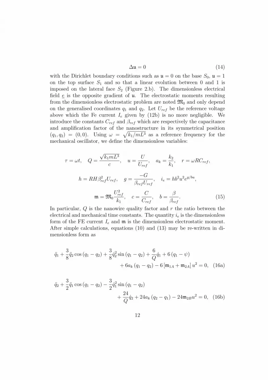
In particular, Q is the nanowire quality factor and r the ratio between theelectrical and mechanical time constants. The quantity ie is the dimensionlessform of the FE current Ie and m is the dimensionless electrostatic moment.After simple calculations, equations (10) and (13) may be re-written in di-mensionless form as

q1 +3

8q2 cos (q1 − q2) +

3

8q22 sin (q1 − q2) +

6

Qq1 + 6 (q1 − ψ)

+ 6ak (q1 − q2) − 6 [m1A + m2A]u2 = 0, (16a)

q2 +3

2q1 cos (q1 − q2) −

3

2q21 sin (q1 − q2)

+24

Qq2 + 24ak (q2 − q1) − 24m2Bu

2 = 0, (16b)

12

rcu + ru (c,1q1 + c,2q2) + hb2u2eg/bu + u − v = 0 (16c)

where c,j = ∂c/∂qj for j = 1, 2. Equations (16) are the nonlinear dimen-sionless governing equations of a cantileverd bi-articulated nanowire in fieldemission. The dynamic behaviour of this NanoElectroMechanical System isdetermined by computing unknown generalised coordinates q1, q2 and u atany time t knowing that all the other quantities are defined. Indeed, variablesm1A (q1, q2), m2A (q1, q2), m2B (q1, q2), c (q1, q2) and b (q1, q2), responsible forthe electromechanical interactions, are determined after solving the indepen-dent dimensionless electrostatic problem (14). As for the remaining electricalor mechanical parameters, they are directly derived from experimental dataand presented in the following section.

3. Values of parameters

In this section, the mechanical and electrical model parameters are definedin order to simulate and study the self-oscillations of a nanowire in fieldemission. It will also specify the order of magnitude of the involved physicalquantities.

3.1. Electromechanical parameters

The dimensions and the material properties of the investigated nanostruc-tures are completely given by the vapor-solid growth mechanism of the sili-con carbide (SiC) nanowires. According to their typical experimental aspectratio, we assume a length L = 10 µm and a circular cross section withdiameter D = 200 nm (giving a area moment of inertia In = πD4/64).The nanowire material being almost equivalent to pure carbon, the den-sity is ρ = 3200 kg/m3 and leads to a mass per unit length expressed asm = ρπ (D/2)2 = 1 × 10−10 kg. Young’s modulus E is determined by fieldemission [7] and is taken as E = 400 GPa. At room temperature and inan Ultra High Vacuum chamber, the mechanical quality factor of a singlyclamped nanowire can reach 160000 [2]. In our simulations, we prefer asmaller less exceptional Q = 20000. The Fowler-Nordheim constants intro-duced in (12b) are experimentally found as H = 2.73 × 10−24 Am2V−2 andG = 4.4145 × 1010 mV−1 [9]. Finally, the SiC nanowires are highly resistiveand their electrical resistance can be taken as R = 1010 Ω.Coming back to the discrete model determined in the previous section, onehas to adapt the given experimental quantities to the actual parameters nec-essary in the governing equation (16). The electric constants R, H and G

13

can directly be used in the model, and the same is true for the mechanicalparameters L or Q. However, the springs stiffnesses and the rigid bars masshave to model the mechanical behaviour of the continuous structure charac-terized by E, In and its mass. Because of our low-dimensional discretization,we will not capture all dynamical experimental features. In this paper, weassume the mass per unit length m to be equal to the experimental one. Inorder to keep a good static model, we impose that the static deflection of thecantilevered nanowire under an end load F0 is equivalent for the continuousand its discrete counterpart. According to [15], it comes simply

F0L3

3EI=L

2

F0L

k1

+L

2

F0L

2k2

. (17)

In order to ensure consistency in the dynamic model, we constrain the ratiobetween the natural frequencies of the clamped-free beam first two modes tobe equivalent in the discrete and continuous model. While this ratio readsω2/ω1 = 6.3 in the continuous case [15], the discrete case is obtained bysolving the set of equations

[

16mL3 1

16mL3

116mL3 1

24mL3

](

q1q2

)

+

[

k1 + k2 −k2

−k2 k2

] (

q1q2

)

=

(

00

)

. (18)

Equation (18) is directly derived from the linearization of the mechanicalequations (10) when no damping, no initial tilting angle ψ and no electro-static forces are considered. By simply respecting the required ratio betweenthe eigenfrequencies of equations (18), we obtain the desired parameter whichare in our specific case k1 = 2.36EI/L and k2 = 2.06EI/L., i.e. a stiffnessratio ak = 0.873.

3.2. Electrostatic variables

The electrostatic variables c, b and m are not obtained directly from theexperimental data but through the electrostatic problem given in section2.2 and they depend also strongly on the nanowire aspect ratio L/D. Thedetermination of these parameters and their related quantities such as r,Uref , βref and Cref , are described in the following.

The electrostatic problem sketched in Figure 2 and accounted for thedimensionless Laplace equation (14) is computed using the finite elementsoftware Cast3m [16]. Solving this equation for different set of generalised

14

angular displacements (q1, q2) yields a discrete map of the dimensionless elec-trostatic quantities in the (q1, q2) space. A polynomial regression is then suffi-cient to define the continuous field enhancement factor b (q1, q2), the electricalcapacitance c (q1, q2) and electrostatic moments m (q1, q2) that are necessaryfor the further numerical analysis of the governing equations.

(a) Outside view of the electrostatic box (b) Nanowire: q1 = 10 and q2 = −4

Figure 4: 3D Finite Element model of the electrostatic boundaries

The vacuum chamber and the boundary surfaces S0, S1 and S01 are gener-ated using 3D elements (20 nodes hexahedral) and are represented in Figure4. According to our kinematics, the cantilevered nanowire of length L ismodelled by two cylindrical bars with diameter D making an absolute angleq1 and q2 with the symmetrical configuration (Figure 4.b). The nanowireapex is represented by a perfect semi-sphere oriented following the upper bardirection. Due to the large scale ratio between the structure and its envi-ronment, electrostatic phenomena will take place mostly in the vicinity ofthe nanowire. As a consequence, the regular mesh has to be refined nearbythe structure but relaxed far from it to keep reasonable computation times.Finally, the solution of the dimensionless Laplace equation (14) is discretizedwith quadratic shape functions in order to correctly model the electrostaticfield evolution near the nanowire apex. The system of linear equations arisingfrom the approximation of (14) is solved using Crout method [17].

A typical electric potential (for q1 = 10 and q2 = −4) is shown inFigure 5.a for a cross-section of the vacuum chamber in the vicinity of thebi-articulated nanowire. Most of the change in the scalar field u takes placeclose to the nanowire. As a consequence, the electric field e = −∇u, is

15

localized all around the structure (Figure 5.b). Due to the large value of theaspect ratio, e is concentrated at its apex as expected (tip effect).

(a) Evolution of electric potential (b) Evolution of electric field magnitude

Figure 5: Electostatic fields nearby the nanowire for q1 = 10 and q2 = −4

According to the dimensionless form of the electrostatic problem, the fieldenhancement factor β is just the magnitude of the electric field at the poleof the semi-sphere while the electric capacitance C is the total charge ofelectrons on the nanowire given by (5). The continuous functions b (q1, q2)and c (q1, q2) are obtained by applying a second order polynomial regressionto their discrete value computed for hundred values of (q1, q2) in the range[−10, 10]. They read

b (q1, q2) = −0.058q21 − 0.074q2

2 + 0.019q1q2, (19a)

c (q1, q2) = −0.105q21 − 0.06q2

2 + 0.082q1q2 (19b)

given that βref = 1.032 × 107m−1 and Cref = 5.192 × 10−17 F for the sym-metrical position (q1, q2) = (0, 0). These electrical functions are maximal forthe symetrical position (0, 0) and decrease quadratically when the nanowiremoves away from it. Note that for practical purpose, the nanowire apex isnot perfectly smooth but made up of several protrusions which are the realfield emitters. According to classical electrostatic theory [13], βref has alsobeen multiplied by 3 to take in account the electric field amplification dueto a hemispherical protrusion. Once these quantities computed, the ratioof time constants reads simply r = ωRCref = 4.458. The voltage referenceUref corresponds to the emergence of the FE current ie inside the emitter.For practical purposes, it is chosen so that ie > 0.01 when U > Uref and is

16

Uref = 400 V in our case. Below this reference value, the FE current givenby the Fowler-Nordheim formula (12b) is negligible due to the exponentialterm e−G/βU . The shape of the dimensionless current Ie in the (q, u) space isgiven in appendix A (Figure 10).

The electrostatic forces derive from the electric field e according to (4).Two particular features can be made out. First, the tip effect pointed outin Figure 5.b introduces strong partial following [18] pulling forces at thenanowire apex. Second, the symmetry of the electric field being broken bythe leaning nanowire, the resultant electrostatic forces are restoring forcestrying to bring the structure back to its symmetrical position. The electro-static moments m1A, m2A and m2B about the two articulations arise fromthe vector product between the electrostatic forces and their distance withthe considered articulation. The coefficients of the second order polynomialregressions of the discrete value of m1A, m2A and m2B computed in the (q1, q2)space are given by

m1A (q1, q2) = 0.026q1 − 0.051q2, (20a)

m2A (q1, q2) = −0.117q1 + 0.054q2, (20b)

m2B (q1, q2) = 0.008q1 − 0.029q2. (20c)

The evolution of the moments is simply linear and their signs are inagreement with the “restoring forces” properties. Moreover, the magnitudeof the moments decreases with the generalised coordinates (q1, q2) down tothe symmetrical position (0, 0) where they cancel.

4. Numerical results

4.1. Computation of the static position

The static equilibrium of the bi-articulated nanowire, later called thebase state, depends on the constant applied voltage V and is obtained bycomputing the fixed points (q0

1, q02, u0) of system (16):

(

q01 − ψ

)

+ ak

(

q01 − q0

2

)

− [m1A + m2A]u20 =0, (21a)

ak

(

q02 − q0

1

)

− m2Bu20 =0, (21b)

v − u0 − hb2u20e

(g/bu0) =0. (21c)

17

In this nonlinear set of equation, the dimensionless electrical and mechan-ical quantities have been defined in Section 3 where the continuous functionsb (q0

1, q02) and m (q0

1, q02) are given by (19) and (20). The base state branch

[19] deriving continously from the base state (q01, q

02, u0) = (ψ, ψ, 0) at for

v = 0, is determined by progressively increasing the control parameter v.The problem f (q0

1, q02, u0) = 0 is solved using Newton-Raphson method for

each step v with the initial guess coming from the previous step.For an initial tilting ψ = 20, we plot the evolution of fixed points

(q01, q

02, u0) against v in Figure 6. Two disctinct behaviours can be clearly

removed from the smooth branches. For a constant applied voltage V lowerthan the voltage reference Vref (i.e. v < 1), the FE current Ie given by theFowler-Nordheim formula (12b) is negligible (no emission). Thus, accord-ing to the electrical equation (21c), the voltage at the nanowire apex readsdirectly u0 = v (Figure 6.b). The restoring electrostatic moments being pro-portional to u2

0, the bi-articulated nanowire is almost quadratically comingback to its symmetrical position (Figure 6.a).

0 0.5 1 1.5 2 2.515

16

17

18

19

20

q 10 , q20 [°

]

v

q10

q20

(a) Mechanical static equilibrium

0 0.5 1 1.5 2 2.50

0.5

1

1.5

u 0

v

(b) Electrical static equilibrium

Figure 6: Evolution of the fixed points(

q01, q0

2, u0

)

against v for ψ = 20

In emission configuration, i.e. for v > 1, the FE current Ie is no longernegligible and increases exponentially with u0, following the Fowler-Nordheimequation. Due to the nanowire electrical resistance, a supplementary volt-age behaving exponentially as Ie appears inside the electrical circuit modelby (21c). As a consequence, the voltage u0 between the nanowire and itsenvironment saturates when increasing v (Figure 6.b). The electrostatic mo-

18

ments saturate as well and the same is true for the evolution of the generalisedcoordinates (q1, q2) (Figure 6.a).

4.2. Stability of the static solutions

We consider the perturbation expansions of the form q (τ) = q0 + ǫq (τ)and u (τ) = u0 + ǫu (τ). Substituting these expansions into the dimensionlessgoverning equation (16) and equating the first power of ǫ, we express thelinearized governing equation around the static equilibrium (q0

1, q02, u0)

q1 +3

8q2 cos

(

q01 − q0

2

)

+6

Qq1 + 6 (q1 − ψ) + 6ak (q1 − q2)

− 6u20

2∑

j=1

[m1A,j + m2A,j] qj − 12u0 [m1A + m2A] u = 0, (22a)

q2 +3

2q1 cos

(

q01 − q0

2

)

+24

Qq2 + 24ak (q2 − q1)

− 48u0m2Bu − 24u20

2∑

j=1

m2B,jqj = 0, (22b)

rcu + ru0

2∑

j=1

c,j qj + (1 + ie,u) u +2

∑

j=1

ie,jqj = 0. (22c)

The dimensionless FE current ie, the electrical capacitance c and electro-static moments m are continuous functions of (q0

1, q02) according to (19) and

(20) obtained from the electrostatic problem. Their partial derivatives withrespect of qj are denoted by the subscript ( ),j and defined at (q0

1, q02). In

particular, derivatives of the FE current are determined with b (q01, q

02) given

in (19) following

ie,j =i0eb2

(

b,jb− gb,ju0

)

, ie,u = i0e

(

2

u0

− g

bu20

)

, i0e = ie(

q01, q

02, u0

)

(23)

and where the subscript ( ),u denotes the derivative with respect to u.

19

Equation (22) may be rewritten in the physical space Z (τ) = [q1 q2 u]T

in the more compact way

MZ (τ) + DZ (τ) + KZ (τ) = 0, (24)

where M, D and K are respectively the mass, damping and stiffness matrix ofthe coupled system (22). The stability of the base state branches (q0

1, q02, u0)

is reached by stating the perturbation Z (τ) in the form

Z (τ) = ϕesτ with ϕ =[

qA1 q

A2 u

A]T, (25)

where the characteristic exponent s = σ + iω leads to the decay rate σ andthe dimensionless frequency ω of the eigenmode ϕ. For practical purpose,the eigenproblem arising from (24) is solved in the phase space W (τ) =[q1 q2 u q1 q2]

T where (24) becomes

BW (τ) − AW (τ) = 0 (26)

and W (τ) = Φesτ so that the computed eigenproblem reads

[sB − A] Φ = 0 with Φ =[

qA1 q

A2 u

A sqA1 sq

A2

]T. (27)

For each value of the control parameter v, the fixed points (q01, q

02, u0) are

computed using (21) so that the linearized governing equation (22) is com-pletely defined. The eigenmodes ϕ and their associated eigenvalues s arethen computed for each v with (27).

For v = 0, the electromechanical system (22) is totally uncoupled giventhat u0 = i0e = 0. The first eigenmodes ϕ

1and ϕ

2are the mechanical modes

of the bi-articulated nanowire of the form ϕ =[

qA1 q

A2 0

]T. These entities are

respectively the classical first and second bi-articulated modes with naturalfrequencies ω1 and ω2 given in Section 3 and where the decay rates σ1 and σ2

are linked to the quality factor Q. The third eigenmode ϕ3

is the electricalmode of the RC circuit formed by the nanowire. This stationary mode(ω3 = 0) is associated with the strong decay rate σ3 = −1/RC.When increasing v, the purely mechanical and purely electrical modes com-bine into electromechanical modes. The electrical contribution u

A in theoscillating modes ϕ

1and ϕ

2grows progressively and the eigenvalues s vary.

In the same way, the mechanical contributions qA1 and q

A2 increase in the

stationary mode ϕ3

but the decay rate σ3 is strongly decreasing. Thus, theinteresting physical phenomenon will be contained in the first mode shapes

20

ϕ1

and ϕ2. In the following, only the natural frequencies and decay rate of

these first two modes are investigated in order to determine the stability ofthe fixed points plotted in Figure 6.

The evolution of the dimensionless eigenvalues s against v for a can-tilevered bi-articulated nanowire in field emission is displayed in Figure 7for the situation of interest. The increase of the natural frequencies showedin Figure 7.a accounts for the strong electrostatic pulling coming from thetip effect in field emission (already expected in Section 3.2). As in Section4.2 for the computation of fixed points, two distinct behaviours are observeddepending on the applied voltage V compared to the field emission referencevoltage Uref . Indeed, the saturation of the voltage u0 illustrated in Figure 6.band due to the FE current emergence is directly reflected in the electrostaticpulling forces, i.e. in the geometric stiffness.

0 0.5 1 1.5 2 2.510.3

10.4

10.5

10.6

ω2

0 0.5 1 1.5 2 2.51.6

1.7

1.8

ω1

v

(a) Evolution of the natural frequencies

0 0.5 1 1.5 2 2.5−2

−1.5

−1

−0.5

0

0.5

1x 10

−3

σ

v

σ1

σ2

unstable

stable

(b) Evolution of the decay rates

Figure 7: Linear vibratory behaviour of the static equilibrium against v

According to the variation of the decay rate given in Figure 7.b, the firstmode ϕ

1becomes linearly unstable for a low voltage v, highlighting thereby

the qualitative agreement between the bi-articulated nanowire modelling andthe experimental observations made in [9]. As above, it is possible to definetwo domains in the decay rate evolution, separated by an inflexion pointlocated at v = 1, indicating that the field emission must be involved inthe destabilization process. A simpler kinematic model (straight nanowire),given in appendix A, may be used to approximate this FE instability mech-anism. Notably, the analytical form of σ (v) points out the interplay of the

21

electromechanical parameters triggering such phenomenon.

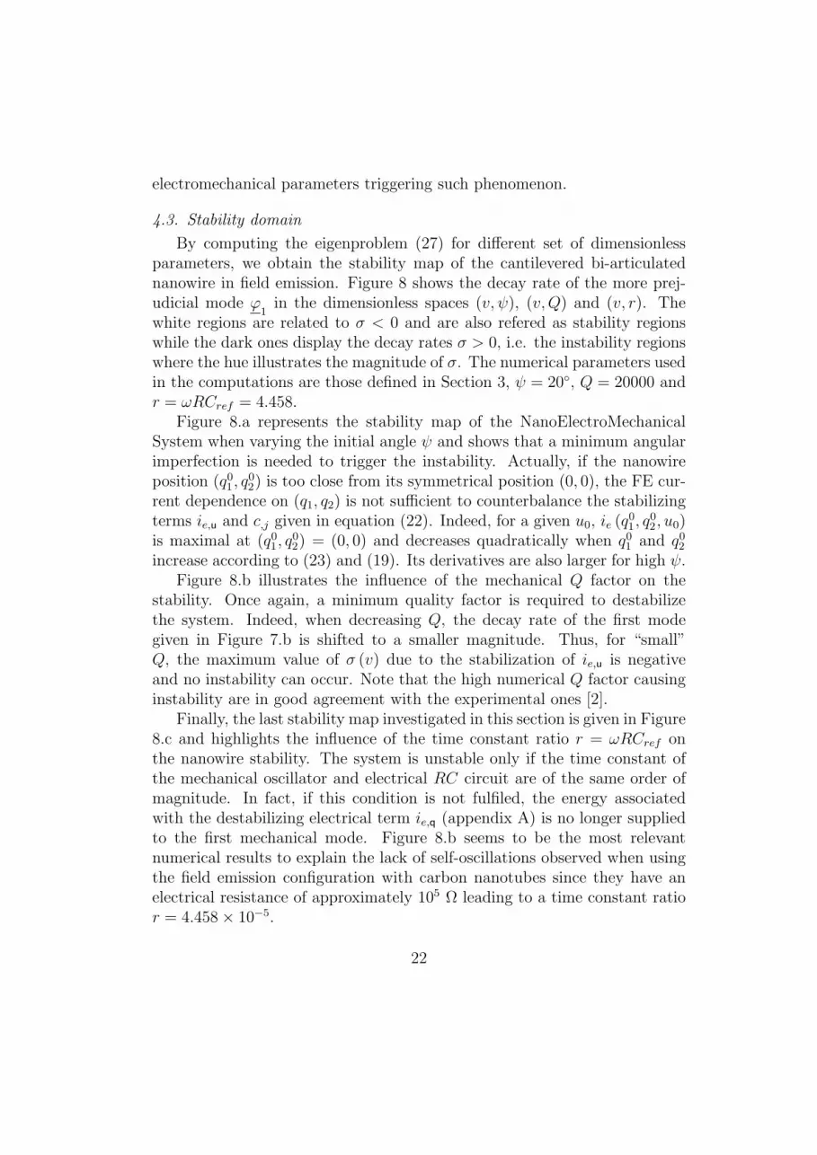
4.3. Stability domain

By computing the eigenproblem (27) for different set of dimensionlessparameters, we obtain the stability map of the cantilevered bi-articulatednanowire in field emission. Figure 8 shows the decay rate of the more prej-udicial mode ϕ

1in the dimensionless spaces (v, ψ), (v,Q) and (v, r). The

white regions are related to σ < 0 and are also refered as stability regionswhile the dark ones display the decay rates σ > 0, i.e. the instability regionswhere the hue illustrates the magnitude of σ. The numerical parameters usedin the computations are those defined in Section 3, ψ = 20, Q = 20000 andr = ωRCref = 4.458.

Figure 8.a represents the stability map of the NanoElectroMechanicalSystem when varying the initial angle ψ and shows that a minimum angularimperfection is needed to trigger the instability. Actually, if the nanowireposition (q0

1, q02) is too close from its symmetrical position (0, 0), the FE cur-

rent dependence on (q1, q2) is not sufficient to counterbalance the stabilizingterms ie,u and c,j given in equation (22). Indeed, for a given u0, ie (q0

1, q02, u0)

is maximal at (q01, q

02) = (0, 0) and decreases quadratically when q0

1 and q02

increase according to (23) and (19). Its derivatives are also larger for high ψ.Figure 8.b illustrates the influence of the mechanical Q factor on the

stability. Once again, a minimum quality factor is required to destabilizethe system. Indeed, when decreasing Q, the decay rate of the first modegiven in Figure 7.b is shifted to a smaller magnitude. Thus, for “small”Q, the maximum value of σ (v) due to the stabilization of ie,u is negativeand no instability can occur. Note that the high numerical Q factor causinginstability are in good agreement with the experimental ones [2].

Finally, the last stability map investigated in this section is given in Figure8.c and highlights the influence of the time constant ratio r = ωRCref onthe nanowire stability. The system is unstable only if the time constant ofthe mechanical oscillator and electrical RC circuit are of the same order ofmagnitude. In fact, if this condition is not fulfiled, the energy associatedwith the destabilizing electrical term ie,q (appendix A) is no longer suppliedto the first mechanical mode. Figure 8.b seems to be the most relevantnumerical results to explain the lack of self-oscillations observed when usingthe field emission configuration with carbon nanotubes since they have anelectrical resistance of approximately 105 Ω leading to a time constant ratior = 4.458 × 10−5.

22

v

ψ [°

]

0.5 1 1.5 2 2.50

5

10

15

20

0

1

2

3

4

5

x 10−4

(a) Influence of an initial tilting(Q = 20000, r = 4.458)

v

Q

0.5 1 1.5 2 2.5

0.5

1

1.5

2

2.5

3

3.5

4

4.5

5x 10

4

0

1

2

3

4

5

6

x 10−4

(b) Influence of the quality factor(r = 4.458, ψ = 20)

v

r

0.5 1 1.5 2 2.510

−1

100

101

102

0

1

2

3

4

5

6x 10

−4

(c) Influence of the time constant ratio(ψ = 20, Q = 20000)

Figure 8: Stability maps of the bi-articulated nanowire in field emission

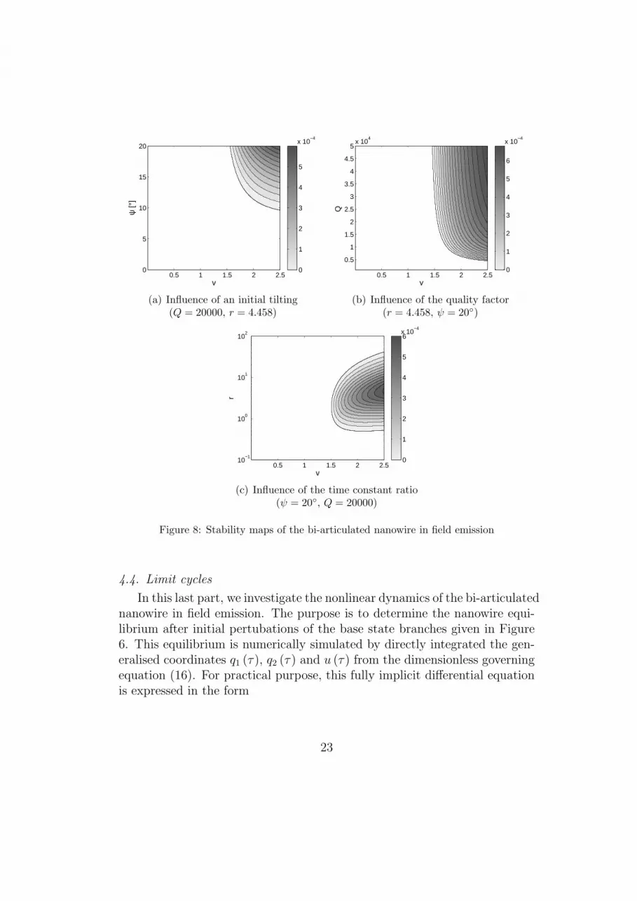
4.4. Limit cycles

In this last part, we investigate the nonlinear dynamics of the bi-articulatednanowire in field emission. The purpose is to determine the nanowire equi-librium after initial pertubations of the base state branches given in Figure6. This equilibrium is numerically simulated by directly integrated the gen-eralised coordinates q1 (τ), q2 (τ) and u (τ) from the dimensionless governingequation (16). For practical purpose, this fully implicit differential equationis expressed in the form

23

12 14 16 18 20 22−8

−6

−4

−2

0

2

4

6

8

φ(τ)

[°]

q(τ) [°]

q1(τ)

q2(τ)

(a) Evolution of q (τ) in the phase space

3.0932 3.0932 3.0932 3.0933 3.0933

x 106

1.242

1.244

1.246

1.248

1.25

1.252

u(τ)

τ

(b) Evolution of U (τ)

0 2 4 6 810

−15

10−10

10−5

100

105

PS

D

ω

q1(τ)

q2(τ)

(c) Frequency spectrum of q (τ))

0 2 4 6 810

−15

10−10

10−5

100

105

PS

D

ω

(d) Frequency spectrum of u (τ)

Figure 9: Steady-state dynamic response for v = 1.55 and ~Y (0) = [θ10 θ20 U0 0.01 0]

f(

τ, Y , Y)

= 0 with Y = [q1 (τ) q2 (τ) u (τ) q1 (τ) q2 (τ)]T . (28)

The differential system (28) is solved for an applied DC voltage v andthe initial conditions q1 (0), q2 (0) and u (0) are the fixed points q0

1, q02 and u0

computed from equation (21). The initial perturbations are applied on theinitial angular velocities φ1 (0) = q1 (0) and φ2 (0) = q2 (0). The electricalquantitites b, c and m are the polynomial regressions of the generalised coor-dinates q1 and q2 given in (19) and (20). Since they are continuous functions,the problem (28) is well defined for any τ .

24

Figure 9 represents the dynamic response of the bi-articulated nanowire infield emission after damping of the transient for a voltage v slightly superior(0.1 %) to the instability threshold given in Figure 7.b. The limit cyclesplotted in the phase space of the Figure 9.a illustrate the nanowire vibrationaround its static equilibrium position. The electromechanical model thusseems to account for the experimental self-oscillations observed in [9]. Figure9.c shows the Power Spectral Density of the steady-state responses q1 (τ) andq2 (τ). At threshold, the mechanical response is harmonic with a frequencyω given by the linear analysis in Figure 7.a.

Figure 9.b displays as well the self-oscillations of the electric voltage u (τ)around its static equilibrium. This time, the secondary harmonic of thesteady-state response is not negligible beside the fundamental one ω. Inagreement with experimental observations, the electrical signal contains a2ω component [9]. Indeed, u (τ) is oscillating with regard to the absoluteposition (q1, q2) and performs also two cycles during a nanowire oscillationperiod. According to the Fowler-Nordheim formula (12b), the FE currentie (τ) is oscillating at the same frequency as u (τ) illustrating the possibilityof DC/AC conversion in this unforced device.

5. Concluding remarks

The study of the basic mechanical phenomena in NEMS and how theycan be best controlled by external parameters is of prime importance in viewof exploiting their possibilities in devices especially because new effects comeinto play at the nanoscale that lead to both complications and opportunities.In particular, the possibilities of self-oscillating nanowires in field emissionshown by Ayari et al. [9] is an important step toward making NEMS activerather than passive devices but deserves further investigations to understandand also control this physical phenomenon.

This paper gives a low-dimensional model to simulate the nonlinear be-haviour of a cantilevered nanowire in field emission. The numerical methodwas presented with a bi-articulated nanowire but can easily be adapted toanother kinematics for obtaining quantitative results rather than qualitativeones. We here highlighted the ins and outs of this electromechanical systemresulting from an original coupling between the nanostructure nonlinear mo-tion, its electrostatic environment and electrical contributions coming fromthe FE current emergence. For a given applied voltage, the linear stabilityof the static equilibrium results from the interplay of the FE current depen-

25

dence on the nanowire absolute position and its dependence on the emitter’svoltage. This interplay, illustrated by the Fowler-Nordheim formula, is verysensitive to external parameters and the same is also true for the emergenceof oscillations. We showed that a minimum initial angular tilting, a highQ factor and a sufficiently high electrical resistance are required to triggerinstability.

For a threshold of applied voltage, the direct integration of the nonlin-ear electromechanical governing equations simulates the limit cycles of thesystem pointing out the possibility of DC/AC conversion in this electrome-chanical device. The dimension of the electromechanical system (16) and itsstrong linearities are sufficient to display complex behaviour of the limit cy-cles when increasing the control parameter v [19]. Future work would focusmore on this original Hopf bifurcation to improve the physical understandingof the self-oscillations.

A. Simplified model for the Field emission instability

A simpler kinematic model can be used to approximate the FE instabil-ity by setting q (t) = q1 (t) = q2 (t) at any time t (straight nanowire case).Even if this basic model contains a poorer kinematics than its two degrees-of-freedom counterpart (specially not taking in account follower forces), itis sufficient to capture properly the mean features of the instability mecha-nism. Deriving from equation (21), the fixed points (q0, u0) of the straightcantilevered nanowire in field emission satisfy the two degrees-of-freedomelectromechanical equations

v − u0 − hb2u20e

(g/bu0) =0 (A.1a)

q0 − ψ − mAu20 =0 (A.1b)

where the dimensionless moment mA (q0) comes from the external electro-static forces applied on the straight nanostructure. Figure 10 displays theevolution of the dimensionless FE current in the (q, u) space given by theFowler-Nordheim formula ie = hb2u2

0e(g/bu0) where b (q0) is computed from

the electrostatic problem with a straight nanowire. The electromechanicalparameters used in Figure 10 are given in Section 3. The linearized governingequations around (q0, u0) derive from (22) and read

26

rcu + (1 + ie,u) u = −ru0c,qq − ie,qq (A.2a)

q +3

Qq +

(

3 − 3ψ − 3u20mA,q

)

q = 6u0mAu (A.2b)

where the subscripts ( ),q and ( ),u respectively represent the derivatives withrespect of q and u. Finally, by expressing the coupled equation (A.2) in the

modal basis Z (τ) = [q (τ) u (τ)]T =[

qA

uA]Tesτ , we find for the decay rate

of the mechanical prevailing mode ϕ1:

σ (v) = − 3

Q+ Γ (v) (A.3a)

with Γ (v) =6ru0mA

r2ω2 + (1 + ie,u)2 × [ie,q − (1 + ie,u)u0c,q] . (A.3b)

0.8 1 1.2 1.4−200

200

0.5

1

1.5

2

2.5

3

uq [°]

i e

Figure 10: Evolution of the dimensionless FE current for the straight nanowire

Relation (A.3) governs the stability of the straight nanowire static equilib-rium against v implicitely through the dependence of the fixed points (q0, u0)given by (A.1)). It can also be qualitatively extended to the decay rate ofthe first mode of the bi-articulated model given in Figure 7.b and serves asa support for the understanding of the stability maps in Figure 8.

27

For v < 1, there is no field emission. The FE current and its partialderivatives ie,q and ie,u are negligible (Figure 10). The only stabilizing termin relation (A.3) comes from the capacitance dependence on q and the decayrate decreases when v increases. This behaviour is in agreement with theevolution of the decay rate of the first mode given in Figure 7.b.

For v > 1, i.e. in field emission configuration, the decay rate (A.3) de-pends on the competition between the destabilizing term ie,q and the stabiliz-ing terms ie,u and c,q. At the begining of the emission, ie,q and ie,u, given by(23), are of the same order of magnitude and the instability can occurred ifc,q is not too large as in Figure 7.b. For higher voltage, since ie,u is increasingfaster than ie,q, the FE destabilizing effect becomes negligible and σ (v) tendsto a maximal value before decreasing again due to the stabilizing terms ie,uand c,q.

References

[1] Ekinci K. L. & Roukes M. L., Nanoelectromechanical systems, Reviewof Scientific instruments, 76 (2005), 061101.

[2] Perisanu S., Vincent P., Ayari A., Choueib M., Purcell S. T., BechelanyM. & Cornu D., High Q factor for mechanical resonances of batch-fabricated SiC nanowires, Applied Physics Letters, 90(2007), 043113.

[3] Jensen K., Kim K. & Zettl A., An atomic-resolution nanomechanicalmass sensor, Nature nanotechnology, 3(2008), 533-537.

[4] Gammel P., Fischer G. & Bouchaud J., RF MEMS and NEMS Technol-ogy, Devices and Applications, Bell Labs Technical Journal, 10(2005),29-59.

[5] Purcell S. T., Vincent P., Journet C. & Binh V. T., Tuning of NanotubesMechanical Resonances by Electric Field Pulling, Physical Review Let-ters, 89(2002), 273103.

[6] Bonard J-M., Kind H., Stockli T. & Nilsson L-O., Field emission fromcarbon nanotubes: the first five years, Solid-State Electronics, 45(2001):893-914.

[7] Perisanu S., Gouttenoire V., Vincent P., Ayari A., Choueib M.,Bechelany M., Cornu D. & Purcell S. T., Mechanical properties of SiC

28

nanowires determined by scanning electron and field emission micro-scopies, Physical Review B, 77(2008) :165434(12).

[8] Perisanu S., Vincent P., Ayari A., Choueib M., Guillot D., BechelanyM., Cornu D., Miele P. & Purcell S. T., Ultra High sensitive detection ofmechanical resonances of nanowires by field emission microscopy, Phy.Stat. Sol., 204(2007) :1645-1652.

[9] Ayari A., Vincent P., Perisanu S., Choueib M., Gouttenoire V.,Bechelany M., Cornu D. & Purcell S. T., Self-Oscillations in Field Emis-sion Nanowire Mechanical Resonators: A Nanometric dc-ac Conversion,Nano Letters, 7(2007) :2252-2257.

[10] Paidoussis M. P., Fluid-Structure Interactions: Slender Structures and

Axial Flow, Volume 1, Academic Press, 1998.

[11] de Langre E., Paidoussis M. P., Doare O. and Modarres-Sadheghi Y.,Flutter of long flexible cylinders in axial flow, J. Fluid. Mech., 571(2007):371-391.

[12] Gibson R. F. , Ayorinde E. E. & Wen Y-F, Vibrations of carbon nan-otubes and their composites: A review Composites science and technol-ogy, 67(2006), 1-28.

[13] Vanderlinde J., Classical Electromagnetic theory, John Wiley & sons,1993.

[14] Bleaney B. I., Bleaney B., Electricity and Magnetism, Volume 1, OxfordSience Publications, 1991.

[15] Blevins R. D., Formulas for natural frequency and mode shape, Volume1 Krieger publishing company, 1979.

[16] Verpeaux P., Charras T. and Millard A., Castem 2000: Une approchemoderne du calcul des structures, Calcul des structures et intelligence

artificielle, Pluralis, Paris, France, 1988, pp 261-271.

[17] Moin P., Fundamentals of engineering. Numerical analysis, CambridgeUniversity Press, 2001.

29

[18] Langthjem M. A. and Sugiyama Y., Dynamic stability of columns sub-jected to follower loads: A survey, Journal of Sound and Vibration,238(2000), 809-851.

[19] Manneville P., Instabilities, Chaos and Turbulence, Imperial CollegePress, 2004.

30