95989_cherkaoui_2021_arch... - archives-ouvertes.fr

HAL Id: tel-03269435https://tel.archives-ouvertes.fr/tel-03269435

Submitted on 24 Jun 2021

HAL is a multi-disciplinary open accessarchive for the deposit and dissemination of sci-entific research documents, whether they are pub-lished or not. The documents may come fromteaching and research institutions in France orabroad, or from public or private research centers.

L’archive ouverte pluridisciplinaire HAL, estdestinée au dépôt et à la diffusion de documentsscientifiques de niveau recherche, publiés ou non,émanant des établissements d’enseignement et derecherche français ou étrangers, des laboratoirespublics ou privés.

Efficient whole brain estimation of the haemodynamicresponse function for TV-regularized semi-blind

deconvolution of neural activity in fMRIHamza Cherkaoui

To cite this version:Hamza Cherkaoui. Efficient whole brain estimation of the haemodynamic response function for TV-regularized semi-blind deconvolution of neural activity in fMRI. Imaging. Université Paris-Saclay,2021. English. �NNT : 2021UPAST022�. �tel-03269435�

https://tel.archives-ouvertes.fr/tel-03269435

https://hal.archives-ouvertes.fr

Thès

e de

doc

tora

tN

NT:

2021U

PAST022

Efficient whole brain estimationof the haemodynamic response

function for TV-regularizedsemi-blind deconvolution of

neural activity in fMRIEstimation efficace de la réponse

hémodynamique cerveau-entier pardéconvolution semi-aveugle, via la

régularisation par variation totale, à partirde données d’IRM fonctionnelle

Thèse de doctorat de l’Université Paris-Saclay

École doctorale n◦ 575: Electrical, Optical, Bio-Physics andEngineering (EOBE)

Spécialité de doctorat: Imagerie et physique médicaleUnité de recherche: Université Paris-Saclay, CEA, CNRS, Inserm,

Laboratoire d’Imagerie Biomédicale Multimodale Paris Saclay, 91401,Orsay, France

Référent: Faculté des sciences d’Orsay

Thèse présentée et soutenue à Paris-Saclay, le 03 mars 2021, par

Hamza CHERKAOUIComposition du jury:

Charles SOUSSEN PrésidentProfesseur, Centrale SupélecJulien MAIRAL Rapporteur & ExaminateurDirecteur de recherche, Inria GrenobleDimitri VAN DE VILLE Rapporteur & ExaminateurProfesseur, Ecole Polytechnique de LausanneFlorence FORBES ExaminatriceDirectrice de recherche, Inria GrenobleMyriam EDJLALI-GOUJON ExaminatriceDocteur, Centre Hospitalier Saint Anne

Direction de la thèse:

Philippe CIUCIU Directeur de thèseChargé de recherche, HDR, CEA NeuroSpinThomas MOREAU Coencadrant de thèse & ExaminateurChargé de recherche, Inria SaclayClaire LEROY Coencadrante de thèse & ExaminatriceChargée de recherche, CEA Service HôspitalierFrédéric Joliot

Nosce te ipsum

— Socrates, 470 - 399 B.C.

© Hamza Cherkaoui 2021

Acknowledgements

The work presented in this thesis was only possible with the support and the help of manypeople. I would like to take the opportunity to express my gratitude.

First I would like to express the deepest appreciation to my supervisors Dr. PhilippeCiuciu, Dr. Claire Leroy and Dr. Thomas Moreau for their continuous support duringthese three years. I really appreciated their patience, the trust and the freedom they gaveme to conduct my work.

I would like to thank Dr. Abderrahim Halimi for the contribution and precious advicehe gave me during this thesis. I would also like to express my gratitude to Dr. BertrandThirion for his kind and regular advice. I am also really grateful to Dr. Nicolas Tournier,Dr. Michel Bottlaender and Dr. Brice Fernandez for your advice during our insightfulmeetings. Thank you for your time, for sharing your knowledge with me.

In addition to the people directly involved in my work, I would like to thank my fellows atParietal, who contributed making the time spent here memorable. To Dr. Pierre Ablin,Thomas Bazeille, Zaccharie Ramzi, Jérôme-Alexis Chevalier and Hugo Richard Icould never thank you enough for spending those difficult periods, you were always here andready to give me some precious advice and laughs. To Dr. Arthur Mensch thank you foryour help and for all the useful conversations we had on optimization in high dimension. ToDr. Kamalaker Reddy Dadi thank you for your help and for all the useful conversationswe had on real data validation, your help was precious. To my former colleagues Dr. ElvisDohmatob, Dr. Mathurin Massias and Dr. Jéromes Dockes you were models. I alsowant to thank all my Metric colleagues, it has been a great pleasure to work with youduring my internship at the begining of my research journey.

Finally I also want to thank my relatives and friends for supporting me during the PhDthesis and in my life in general. To my parents and my sisters, I thank you for always beinghere for your kindness and support.

iii

Contents

Notation vii

General Introduction 1

I Context 7

1 Introduction to fMRI 91.1 Introduction to neuroscience . . . . . . . . . . . . . . . . . . . . . . . . . . . 101.2 Principle of Magnetic Resonance Imaging (MRI) . . . . . . . . . . . . . . . . 131.3 Introduction fMRI . . . . . . . . . . . . . . . . . . . . . . . . . . . . . . . . . 191.4 Neurovascular coupling in fMRI . . . . . . . . . . . . . . . . . . . . . . . . . 231.5 Chapter conclusion . . . . . . . . . . . . . . . . . . . . . . . . . . . . . . . . 27

2 How to segregate the vascular and neuronal components in fMRI? 292.1 Introduction to the General Linear Model (GLM) . . . . . . . . . . . . . . . 292.2 HRF estimation with fixed neural activity . . . . . . . . . . . . . . . . . . . 312.3 Neural activity estimation with fixed HRF . . . . . . . . . . . . . . . . . . . 342.4 Joint estimation of the neural activity and the neurovascular coupling from

BOLD signal . . . . . . . . . . . . . . . . . . . . . . . . . . . . . . . . . . . . 372.5 Conclusion . . . . . . . . . . . . . . . . . . . . . . . . . . . . . . . . . . . . . 38

3 TV problems minimization with iterative algorithms 393.1 Introduction to regularization in optimization . . . . . . . . . . . . . . . . . 393.2 Solving a TV regularized problem . . . . . . . . . . . . . . . . . . . . . . . . 423.3 Performance comparison . . . . . . . . . . . . . . . . . . . . . . . . . . . . . 473.4 Chapter conclusion . . . . . . . . . . . . . . . . . . . . . . . . . . . . . . . . 50

II Methodological Developments 53

4 TV problems minimization with learned algorithms 554.1 Introduction to TV regularization in 1D . . . . . . . . . . . . . . . . . . . . 564.2 Solving a TV regularized problem . . . . . . . . . . . . . . . . . . . . . . . . 57

v

vi Contents

4.3 Performance comparison . . . . . . . . . . . . . . . . . . . . . . . . . . . . . 694.4 Conclusion . . . . . . . . . . . . . . . . . . . . . . . . . . . . . . . . . . . . . 72

5 Contribution to neurovascular disentangling 755.1 Sparsity-based blind deconvolution of neural activation signal in fMRI . . . 765.2 fMRI BOLD signal decomposition using a multivariate low-rank model . . . 815.3 Conclusion . . . . . . . . . . . . . . . . . . . . . . . . . . . . . . . . . . . . . 88

6 Multivariate joint estimation neural activity HRF 896.1 Introduction . . . . . . . . . . . . . . . . . . . . . . . . . . . . . . . . . . . . 906.2 Multivariate low-rank decomposition of the BOLD signal . . . . . . . . . . . 906.3 Model Validation . . . . . . . . . . . . . . . . . . . . . . . . . . . . . . . . . 976.4 Clinical validation at the population level . . . . . . . . . . . . . . . . . . . . 1096.5 Conclusion . . . . . . . . . . . . . . . . . . . . . . . . . . . . . . . . . . . . . 113

7 Clinical application 1157.1 Analysis of the Synchropioid cohort . . . . . . . . . . . . . . . . . . . . . . . 1157.2 Summary . . . . . . . . . . . . . . . . . . . . . . . . . . . . . . . . . . . . . . 121

General Conclusion and Perspectives 123Contributions . . . . . . . . . . . . . . . . . . . . . . . . . . . . . . . . . . . . . . 123Limitations & Perspectives . . . . . . . . . . . . . . . . . . . . . . . . . . . . . . . 125

Appendices 129

A Résumé en français (Abstract in French) 131

Bibliography 139

Notation

In this manuscript, the mathematical notation follows general typographical conventions.

Symbol Description

N The set of Natural numbers.

R The set of Real numbers.

α Lower-case letters denote scalars.

xi subscript i denotes the ith entry of vector x.

x Lower-case bold letters denote vectors.

A Upper-case bold letters denote matrices.

A> or x> Matrix (A) or Vector (x) transpose is represented by an exponent >.

× Cross product.

‖A‖F The Frobenius norm of a matrix defined as ‖A‖2 =√∑mi=1

∑nj=1 |Ai,j |2.

‖x‖2 The `2-norm of a vector defined as ‖x‖2 =√∑m

i=1 x2i .

‖x‖1 The `1-norm of a vector defined as ‖x‖1 =∑mi=1 |xi|.

‖x‖0 The `0 pseudo-norm of a vector defined as ‖x‖0 =∑mi=1 1xi 6=0

v ∗ a ∈ R1×T The convolution of two signals a ∈ R1×(T+L−1) and v ∈ R1×L

v ∗ A ∈ RP×T The convolution of each line of A ∈ RP×(T+L−1) with v ∈ R1×L

V ∗ A ∈ RP×T The convolution of each line ofA ∈ RP×(T+L−1) with the correspondingline of V ∈ RP×L

∇x ∈ RT−1 the first-order difference operator such as (∇x)i = xi − xi−1, ∀i ∈{2, . . . , T}

Γ(x) The Gamma function evaluated on x ∈ R defined as Γ(x) =∫∞0xt−1e−xdx.

N (µ,V ) Multivariate normal distribution with mean µ and covariance matrixV .

Γ0(RT ) The set of convex, proper, lower semi-continuous functions on RT →R ∪+∞.

vii

General Introduction

Context & Motivations

F unctional magnetic resonance imaging (fMRI) non-invasively records brain activityby dynamically measuring the blood oxygenation level-dependent (BOLD) contrast. The

latter indirectly measures neural activity through the neurovascular coupling [Ogawa et al.,1992]. This coupling is usually characterized as a linear and time-invariant system and thussummarized by its impulse response, the so-called haemodynamic response function(HRF) [Bandettini et al., 1993, Boynton et al., 1996]. The estimation of this response is ofprimary interest for clinicians: a change in the haemodynamic response could be linked tothe pharmacological mechanism of a drug [Do et al., 2020], the effect of normal aging [Westet al., 2019] or the consequence of a neuropathological process [Asemani et al., 2017]. Thus,the HRF could be considered as a precious biomarker to investigate the neurovascularfunction of the brain in healthy or pathological condition. Moreover, its estimation alsolinks the observed BOLD signal to the underlying neural activity, which can in turn beused to better understand cognitive processes. Several methods have been designed toestimate the haemodynamic response function in the context of task-related fMRI (tfMRI).In this setup, the participant is engaged in an experimental paradigm (EP) during theimaging session, which typically alternates between rest and task periods [Friston et al.,1998a, Ciuciu et al., 2003, Lindquist and Wager, 2007, Pedregosa et al., 2015] during whichthe participant is submitted to sensorymotor stimuli or more cognitively demanding tasks.Commonly, supervised HRF estimation methods fit a model to explain the observed BOLDsignal from the EP, namely binary input signal corresponding to stimulus onsets [Ciuciuet al., 2003, Lindquist and Wager, 2007, Vincent et al., 2010, Pedregosa et al., 2015]. Alimitation of these approaches is that the EP is used as a surrogate for the neural activity.Therefore these methods cannot be used on resting-state fMRI data (rs-fMRI), where no EPis available. On the other hand, a long-standing literature on fMRI deconvolution methodshas emerged since the late 90s to uncover the underlying activity-inducing signal at thefMRI timescale of seconds [Glover, 1999, Gitelman et al., 2003, Hernandez-Garcia andUlfarsson, 2011, Khalidov et al., 2011]. Importantly, a foundational work [Karahanoğluet al., 2013] has proposed a spatio-temporal model of the underlying activity-inducing signalincluding both temporal and spatial sparsity-based regularization. By doing so, the recoveredneural activity profiles are used to characterize functional networks, hence converging tothe original approach proposed by Wu et al. [2013] that reveals functional networks from

1

2 General Introduction

deconvolved BOLD signals. Alternatively a recent work [Farouj et al., 2019] has suggestedto simultaneously estimate both the neural activity and the HRF profile with a limitedparameterization. This approach is often referred to as semi-blind deconvolution schemes ofthe BOLD signal. Farouj et al. [2019] relies on the hypothesis of a constant block signal forthe neural activity as initially proposed in Karahanoğlu et al. [2013]. However in [Faroujet al., 2019], the authors are able to infer the haemodynamic parameters to deal with themagnitude and delay ambiguities between the neural input and the HRF.

Contributions

I n this thesis we propose a novel approach to disentangle the activity-inducing signal (neuralactivation signal) from the neurovascular coupling (HRF) for both task-related and resting-

state fMRI (tfMRI and rs-fMRI, respectively). In short, the general idea is to define a modelthat is able to separate these two components at the scale of the whole brain, along with asuitable optimization algorithm as a means to perform parameter estimation in an efficientway. After an introduction to neuroimaging techniques, in particular to magnetic resonanceimaging (MRI), as well as to the mechanisms underlying the BOLD signal measured infMRI (chapter 1), we present, in chapter 2, the state-of-the-art methods that estimate theHRF or the neural activity signals from fMRI data. In particular, we focus on the seminalwork introduced by Karahanoğlu et al. [2013] that models the neural activation signal as apiecewise constant block time series. This hypothesis is especially relevant for tfMRI wherethe EP has such block structure and potentially the neural signals too, but it also makessense in the context of rs-fMRI as a means to regularize the spontaneous neural activity.

This piecewise constant hypothesis on the neural inputs is enforced using 1-dimensional (1D)Total Variation (TV) regularization which promotes sparsity of the first-order derivative ofthe neural signal and thus leads to block-shaped signals. The resolution of such deconvolutionproblem with TV regularization can be computationally expensive. After a review and abenchmark of classical approaches to solve 1D TV-regularized problems (chapter 3), we the-oretically compare the performances of the analysis vs synthesis approaches in chapter 4,and show that the analysis algorithms can be much more efficient than their synthesiscounterparts for the problems under study. In this work, we also propose a way to performdifferentiable algorithm unrolling [Gregor and Le Cun, 2010] for proximal gradientdescent (PGD) with TV-regularized optimization problems by either directly computing thegradient of the TV proximal operator with an analytic formula (LPGD-Taut) or computingit with a nested unrolled algorithm (LPGD-LISTA). Comparison on real fMRI data showspromising results for learned optimization algorithm based on this unrolling compared toiterative algorithms.

In order to study the haemodynamic response over the whole brain, we first propose toestimate voxelwise HRFs (first part of chapter 5). This univariate method is based on the sameblock hypothesis for the neural activity and introduces a simplistic but novel modeling for theHRF. The haemodynamic response is modeled as a time dilated version of the canonicalHRFvref(t), whose definition relies on the difference between two Gamma distributions Fristonet al. [1998a]. This parameterization allows us to summarize the HRF with a single dilationparameter δ. One limitation of this contribution is its massively univariate aspect. Indeed,as we estimate both the neural input signal and the HRF, the total number of parameters in

General Introduction 3

this model is similar to the number of scans which could lead to overfitting. To cope withthis issue, we propose two contributions [Cherkaoui et al., 2019b, 2020a] that extend theprevious model in a multivariate setting in order to capture more efficiently the neurovascularcoupling. In the second part of chapter 5, we introduce K temporal components andtheir corresponding spatial maps to encode the neural activity signals and respectivelylocalize their contribution to the measured BOLD fMRI data. Moreover, in Cherkaoui et al.[2020a], we extend this model to estimate the neurovascular coupling over the whole brainas a time dilated HRF for each region from a predefined brain parcellation (chapter 6).At the subject level, we demonstrate that the estimated neural activity spatial mapsare related to meaningful functional networks. To assess the significance of thisapproach at the population level, we statistically demonstrate that a pathology like stroke ora condition like normal brain aging induce longer haemodynamic delays in certain brain areasand that this haemodynamic feature may be predictive of the individual status in a machinelearning (classification) task. Moreover, we investigate in chapter 7 the usefulness of ourmethod in a clinical context. We analyze PET/fMRI imaging data recorded simultaneouslyon a PET/MR system installed at the Service Hospitalier Frederic Joliot (CEA/DRF/Joliot,Orsay) in the context of a protocol called Synchropioid. The latter aims to understand thepharmacological mechanism of the buprenorphine – an analgesic drug – on the brain inorder to understand and unveil its side effects like some habituation or the need to rapidlyincrease the dose to obtain an analgesic effect in some specific patients. Using the PETdata, we aim to respectively localize where the buprenorphine is fixated in the brain andin which brain regions it is mostly concentrated. Next, from the concomitantly recordedrs-fMRI data, our objective is to study the effect of the drug on the haemodynamic system,in particular whether it impacts the HRF profile and to what extent the observed effect,if any, is consistent with our findings in PET imaging. In short, our preliminary resultson four subjects (two healthy volunteers treated with the analgesic dose vs two healthycontrols) indicate that the buprenorphine is mostly concentrated in the Putamen (subcorticalnucleus) and in the Insula and that these regions are mostly affected by a deceleration of theneurovascular coupling, observed through longer time-to-peaks in the HRFs.

Thesis Outline

This dissertation is organized as follows:

Chapter 1: Introduction to fMRI proposes an introduction to the neuroscience and theirmost common imaging techniques. We focus more specifically on the MRI, next on functionalMRI and finally introduce the neurovascular coupling along with the definition of the HRF.

Chapter 2: How to segregate the vascular and neuronal components in fMRI? introducesthe state-of-the-art approaches to disentangle the vascular coupling from the neural activityinvolved in the fMRI signal.

Chapter 3: TV problems minimization with iterative algorithms proposes to summarizethe methods used to solve the optimization problem that involved the Total Variationregularization, as this regularization is central in our contribution to estimate the HRF.

Chapter 4: TV problems minimization with learned algorithms introduces our novelapproach to solve more efficiently the optimization problem that involved the Total Variation

4 General Introduction

regularization based on neural network.

Chapter 5: Contribution to neurovascular disentangling proposed to expose our twofirst contributions done to disentangle the vascular coupling from the neurovascular coupling.

Chapter 6: Multivariate joint estimation neural activity HRF exposes our majorcontribution to disentangle the vascular coupling from the neurovascular coupling in amultivariate fashion for the whole brain.

Chapter 7: Clinical application proposes to apply our multivariate disentangling method tothe Synchropioid cohort to investigate the pharmacological mechanism of the buprenorphine.

Publications

Articles submitted in Peer-Reviewed Journals

Hamza Cherkaoui, Thomas Moreau, Abderrahim Halimi, Claire Leroy and Philippe Ciuciu.Multivariate semi-blind deconvolution of fMRI time series. under review at NeuroImage

International Conferences Paper Presented with Reading Committee

and Proceedings

Hamza Cherkaoui, Jeremias Sulam and Thomas Moreau. Learning to solve TV regularized

problems with unrolled algorithms.. Proceedings of the 34th Conference on Neural InformationProcessing Systems (NeurIPS), Virtual, 2020. Poster.

Hamza Cherkaoui, Thomas Moreau, Abderrahim Halimi and Philippe Ciuciu. fMRI

BOLD signal decomposition using a multivariate low-rank model.. Proceedings of the 27thEuropean Signal Processing Conference (EUSIPCO), A Coruña, Spain, 2019. Oral.

Hamza Cherkaoui, Thomas Moreau, Abderrahim Halimi and Philippe Ciuciu. Sparsity-based blind deconvolution of neural activation signal in fMRI. Proceedings of the IEEEInternational Conference on Acoustics, Speech and Signal Processing (ICASSP), Brighton,United Kingdom, 2019. Poster.

Hamza Cherkaoui, Loubna El Gueddari, Carole Lazarus, Antoine Grigis, Fabrice Poupon,Alexandre Vignaud, Sammuel Farrens, Jean-Luc Starck and Philippe Ciuciu. Analysis vs

synthesis-based regularization for combined compressed sensing and parallel MRI reconstruc-

tion at 7 Tesla.. Proceedings of the 26th European Signal Processing Conference (EUSIPCO),Rome, Italy, 2018. Poster.

Abstract in peer-reviewed international conferences without proceedings

Hamza Cherkaoui, Thomas Moreau, Abderrahim Halimi, Claire Leroy and PhilippeCiuciu. Data-driven haemodynamic response function estimation: a semi-blind multivariate

deconvolution of the fMRI signal. Organization for Human Brain Mapping, Virtual, 2020.Poster.

5

Part I

Context

7

Chapter 1

Introduction to fMRI

Chapter Outline

1.1 Introduction to neuroscience . . . . . . . . . . . . . . . . . . 101.1.1 Description of the brain . . . . . . . . . . . . . . . . . 101.1.2 Neuroscience and the usual neuroimaging modalities. . . . . . . 11

1.2 Principle of Magnetic Resonance Imaging (MRI) . . . . . . . . . . . 131.2.1 Signal-to-noise-ratio (SNR) . . . . . . . . . . . . . . . . 141.2.2 Polarization using radio-frequency (RF) waves . . . . . . . . . 151.2.3 Relaxation . . . . . . . . . . . . . . . . . . . . . . 151.2.4 Weighting contrast . . . . . . . . . . . . . . . . . . . 151.2.5 Measuring the FID signal . . . . . . . . . . . . . . . . 161.2.6 Spatial encoding . . . . . . . . . . . . . . . . . . . . 171.2.7 Image reconstruction . . . . . . . . . . . . . . . . . . 181.2.8 MRI in clinical practice . . . . . . . . . . . . . . . . . 19

1.3 Introduction fMRI. . . . . . . . . . . . . . . . . . . . . . 191.3.1 Principle of Functional MRI (fMRI). . . . . . . . . . . . . 191.3.2 Classical fMRI preprocessing . . . . . . . . . . . . . . . 211.3.3 fMRI acquisition. . . . . . . . . . . . . . . . . . . . 22

1.4 Neurovascular coupling in fMRI . . . . . . . . . . . . . . . . . 231.4.1 Introduction to the neurovascular coupling and its modeling . . . . 231.4.2 Clinical application . . . . . . . . . . . . . . . . . . . 25

1.5 Chapter conclusion . . . . . . . . . . . . . . . . . . . . . 27

I n this chapter we introduce the brain and its structure and give a general introduction toneuroscience before focusing more specifically on functional Magnetic Resonance Imaging

(fMRI), the imaging technique dedicated to probe brain function both at rest and duringtask performance. In regards to the imaging technique, we will first describe the bloodoxygenated level dependent (BOLD) effect at the origin of the signal measured in fMRI,and then will cover the way the data is collected from an acquisition perspective up to theclassical preprocessing pipeline. Finally, we will focus on the fMRI signal and more speciallyon the neuro-vascular coupling involved in the signal generation, how to model it and howthis coupling can be relevant as a biomarker for further statistical analysis.

9

10 Introduction to fMRI

1.1 Introduction to neuroscience

1.1.1 Description of the brain

As the remaining of the on manuscript focus on functional Magnetic Resonance Imaging(fMRI), its signal (the BOLD contrast) and more specifically on the neurovascular couplingwhich is at the core of the fMRI signal generation, we first briefly propose a generalintroduction to the brain to provide a meaningful context.

The brain structure

The brain is part of the central nervous system and is composed of three major parts: (i) thebrainstem that makes the junction with the rest of the nervous system, (ii) the cerebellumthat regulates motor movements and coordinates voluntary movements and the neocortexthat is notably responsible for the higher cognitive functions such as the memory, the learningor the language for example.

In the brain, we can differentiate two major types of cells: the glial cells and the neurons.Briefly speaking, neurons are responsible for all sensory-motor and cognitive functions whilethe glial cells are responsible for supporting and protecting the neurons. The brain containsabout 86 billion neurons. The neurons are connected one another in complex structure, theneuropil, which defines specific functionality. The population of neurons is densely connectedand mainly located in the gray matter. The main second component of the brain tissuesis the white matter where lie the myelinated fiber bundles of neuronal axons. Myelin is alipid-rich substance that insulates axons to allow for a better propagation of electric spikesand thus connects distant gray matter regions across the whole brain.

This mechanism of distant neuronal connections through the white matter enables efficienthigh cognitive functions in the brain.

Introduction to the neuron

The neuron contains a nucleus inside the cell body. Neurons are connected to each otherby extensions at the level of their cell bodies named dendrites and their axon terminals,namely synaptic endings. The axon is surrounded by myelin sheath and schwann cell whichare at the base of the white matter, see illustration Figure 1.1-1 (b) to observe a schema ofmultipolar neuron. There exists a hundred of different types of neurons in the brain withspecific message-carrying abilities, Figure 1.1-1 (a) is an illustration of staining of pyramidalneurons [Del Río and De Felipe, 1994] in the primate neocortex with which we notice thelong axon and the dendrite connecting the neurons to each others.

The signal spreading across neuron’s membranes from the synapse to the dendrites ispartly electrical and partly chemical. When a neuron is excited on its axon terminals fromothers neurons’ dendrites, if the overall voltage exceeds a certain threshold the neuronitself will in turn produce an electrochemical spike, called action potential, that permitsto propagate the signal to other neurons. By cascading these elementary action potentialsacross the vastness of neural connections, the information flow may circulate at high speed inthe whole brain to synchronize distant brain regions and thus underpin cognition functions.

1.1. Introduction to neuroscience 11

(a)

Dendrite

Axon

Nucleus

Myelin sheathSchwann cell

Node of Ranvier Axon Terminal

(b)

Figure 1.1-1 – (a) Multipolar neuron photo in the primate neocortex - (b) Mul-tipolar neuron illustration. In (a) we display SMI32-stained pyramidal neurons whichallows us to observe the complex connection produce by the axon terminals and dendrites. In(b) we propose a schematic illustrate of the structure of a neuron from the dendrite attachedto the cell body with its nucleus at its center, to the axon, envelopped with a myelin sheathproduced by the Schwann cell separated by the node of Ranvier, up to the axon terminal.

We briefly focus on the glial cells, as they have a determinant role for the remaining forour work. As explained, those cells support and protect the neurons to ensure their properworking. We can distinguish four different types, see Figure 1.1-2:

• Ependymal are responsible for the production of cerebrospinal fluid that surround thebrain and protects it from shocks.

• Astrocytes have numerous different roles. Among them they provide neurons withnutrients and they serve as intermediaries in neuronal regulation of blood flow.

• Oligodendrocytes provide support and insulation to axons by creating the myelin sheath(the white matter).

• Microglial are macrophages that actively participate in immune defense of the brain.

In the present work, defining a model to capture the vascular coupling to the neuralactivation signals is indirectly interested in astrocytic activity. Therefore, the role of astrocytesin modulating the cerebral blood flow (CBF) to the metabolic demand of brain activity is offundamental importance to provide an appropriate and consistent energy supply to supportbrain function.

1.1.2 Neuroscience and the usual neuroimaging modalities

Modern neuroscience studies the brain in healthy or pathological condition to understandeither the cognitive functions (language, consciousness, memory, time perception, etc.) ordiseases’ mechanisms in neurogenerative pathology (e.g. Parkinson, Alzheimer). To thisend, modern neuroscience heavily relies on neuroimaging, both structural and functional toanalyse the brain structure and function. To that aim, several imaging techniques can beemployed (see list in Figure 1.1-3), some of them being more sensitive to the timing of eventsin the brain with a millisecond temporal resolution (EEG, MEG), while others (i.e. MRI


Neuron

Microglialcell

OligodendrocyteSynapse

Axon

Capillary

Axon

Astrocytes

Pia mater

Astrocytes

Astrocyte’s endfoot

Astrocyte

Figure 1.1-2 – Illustration of the differenttypes of Glial cells. The figure displays thefour different types of glial cells present in thebrain: the pia mater cells, astrocytes (withtheirs endfoot), the oligodendrocytes and themicroglial cells. The neurons are representedwith theirs synapses and axons and the capil-lary in red. Source: Atlas de neuroscienceshumaines de Netter Felten and Shetty [2011].

and fMRI) have a better ability to probe brain structure and localize which brain regionsare engaged during task performance or even at rest due to a millimetric spatial resolution.Last but not least, nuclear imaging techniques like PET may access molecular sensitivityto decipher metabolic activity (e.g. ATP synthesis or glucose consumption) that cannot bereached using non-invasive and non-ionizing techniques such as fMRI.

Figure 1.1-3 – Imaging modalitiesrepresented along the two axesdescribing the spatial and tem-poral resolution. Additionally,the color indicates the degreeof invasiveness. The most com-mon imaging techniques in neuros-cience: the Electroencephalography(EEG), the Magnetoencephalography(MEG), the structural Magnetic Res-onance Imaging(MRI) and the func-tional Magnetic Resonance Imaging(fMRI) and the nuclear imaging mod-alities PET and SPECT, namelyPositron Emission Tomography andSingle Photon Emission Computer-ized Tomography. Note the of tem-poral resolution of the fMRI modalitywhile being non-invasive.

Neuroimaging techniques• Electroencephalography (EEG) is a time-resolved modality (a millisecond time resolution)

that records in a non-invasive manner the voltage fluctuations, resulting from the neuralactivity (i.e. local field potentials as a marker of post-synaptic activity) on the scalpsurface [Logothetis et al., 2001]. An EEG acquisition is obtained by placing an headsetmade of 64 to 256 electrodes to record the potential fluctuations in the range ofmicrovolts (µV).

• Magnetoencephalography (MEG) is a time-resolved modality (a millisecond time resolu-

1.2. Principle of Magnetic Resonance Imaging (MRI) 13

tion) that records in a non-invasive manner the fluctuations in magnetic fields generatedby the neuronal activity in the cortex, resulting from the neural activity on the scalpsurface. A MEG acquisition is obtained by placing the head of the subject insidea recording large and fixed helmet. As the recorded magnetic fields are of very lowintensity (in the order of 10−13 Tesla), the MEG machine is installed within a Faradaycage to remove the contribution of external magnetic perturbations due for instance tothe Earth’s magnetic field.

• Positron Emission Tomography (PET) is an imaging technique that localizes a radio-tracer to quantify various physiological activities such as neurotransmission, metabolicprocesses or blood flow. The radiotracer is injected at a tracer dose which corres-ponds to a small concentration that does not noticeably influence the pharmacology orpharmacokinetics of the process being imaged. This radiotracer is marked by an iso-tope (carbon, fluorine, nitrogen, oxygen, etc.) that emits positrons whose annihilationproduces the emission of two photons. The detection of the trajectory of those photonsby external detectors positioned at different orientations in the PET camera localizesthe emission position and therefore the concentration of the radiotracer in the brain.

• Structural Magnetic Resonance Imaging (MRI) is a non-invasive and non-ionizingimaging technique that images the morphological structure of the brain (gray andwhite matter, cerebrospinal fluid, skull, etc.) by manipulating the magnetization of thehydrogen atoms contained in the water molecules. This process involves a polarizationstep which consists in deviating the spins of hydrogen atoms from their equilibrium andthen measuring how fast they return to this equilibrium state. Because the differenttissues present in the brain have different relaxation properties, one may create acontrast between these tissues and create precise images that reflect the anatomy. Theprinciple of MR data acquisition and image reconstruction are given in section 1.2.

• Functional Magnetic Resonance Imaging (fMRI) is a non-invasive techniques thatrecords indirectly the neural activity by taking advantage of the magnetic fluctuationsinduced by the level of oxygenation in the blood. Its temporal resolution ranges around1 to 2 seconds and its spatial resolution is nowadays around 1.5 mm isotropic. Thistechnique thus captures low frequency activity compared to EEG and MEG. As fMRIdata is at the core of this thesis, we will dedicate section 1.3 to its introduction, fromthe origin of the measured signal to the common preprocessing pipeline and the typeof acquisitions one usually meets.

1.2 Principle of Magnetic Resonance Imaging (MRI)

Magnetic Resonance Imaging is a non invasive imaging technique widely used in the medicalfield, mainly to probe soft tissues in the human body. The principle of MRI is based onthe spin property of some molecules, such as hydrogen, phosphorus or sodium, was firstdescribed in 1940 [Bloch et al., 1946], which have a non-zero magnetic moment due to theireven number of nucleons (protons and neutrons).

As the water molecules are the most prominent in the human body, one can easilymanipulate the spins of hydrogen atoms embedded in water molecules to create MR images.In essence, the vast majority of MRI exams typically produce maps of “water density” infirst approximation.


A MR system actually relies on three major components:

• A large static magnetic field, denoted B0 (e.g. 3 Tesla), which gives the MRI machineits distinctive aspect, cf. Figure 1.2-4. The role of this static B0 field is to align allhydrogen atoms present in water molecules with its main direction.

• An organ-specific coil that is used to deliver the radio-frequency waves at the Larmorfrequency (ω0 = γB0 and γ = 42.58MHz/T defines the gyromagnetic ratio for thehydrogen atom) to generate the resonance phenomenon and collect in return the MRsignal. In the MR field, on refer this radio-frequency wave as the B+

1 (transmit) andB−1 (receive) fields. For instance, the coil may have a birdcage form in neuroimagingand can comprise a large number of channels to boost the signal-to-noise-ratio (SNR).The coil is also tuned for the type of imaging underwent. This means that a coil usedfor proton imaging cannot be used for Sodium imaging as the gyromagnetic ratios γdiffer between the two atoms.

• The magnetic field gradients system that allows for the spatial encoding of the MRsignal into the k-space or the spatial frequency domain. This encoding can be done in2D or in 3D leading to 2D and 3D imaging respectively. Most of MR pulse sequencesrely on 2D imaging for the sake of speed. Hence, 3D volumes are then reconstructedby stacking multiple 2D slices.

Figure 1.2-4 – MRI scanner of 3T. Ex-ample of a 3T MRI system installed atNeurospin (CEA Saclay, France) to performstructural or functional neuroimaging.

1.2.1 Signal-to-noise-ratio (SNR)

The image resolution in MRI depends on several factors but the larger the SNR, thehigher the resolution one can reach. As B0 contributes to the gain in SNR more thanlinearly (SNR ∝ B1.65

0 ), higher image resolution is expected at 7 Tesla compared to 3 and1.5 Tesla. Currently, the more powerful scanner for clinical usage is at 10.5T in the CMRRcenter, Minneapolis (MN, USA). However, the 11.7T Iseult scanner installed at NeuroSpin1

should be available for human exams in 2022 after a 1-year safety check period. As a gain inimage resolution requires longer acquisition times, most often the MR exams are performedat millimetric resolution to keep scan time compatible with clinical routine. This allowsthe physician to maintain a scan time close to a few minutes per imaging contrast. Higher

1see https://www.cea.fr/english/Pages/News/Iseult-MRI-Magnet-Record.aspx


resolution imaging (e.g. 600µm isotropic) can be performed using dedicated accelerationtechniques, as detailed hereafter.

1.2.2 Polarization using radio-frequency (RF) waves

During the acquisition, the aligned spinning molecules of hydrogen are polarized with a RFwave (i.e. B+

1 magnetic field delivered through a transmit coil) which produces a tilt of thespinning molecules. The frequency of the RF wave must be equal to the Larmor frequencyof the hydrogen atoms to tilt them in the plan (say (Oxy)) which is orthogonal to the B0

field direction (Oz).

1.2.3 Relaxation

Once the RF pulse is stopped, the polarized molecules lose their excess of energy by emittingback a magnetic echo to return to their equilibrium. This process is accompanied witha double relaxation, the longitudinal relaxation Mz(t) that describes the regrowth of themagnetization along (Oz) and the transverse relaxation Mxy(t) that describes how fast themagnetization vanishes in (Oxy). The corresponding dynamics are given by the simplestform of the Bloch equations:

Mz(t) = M0(1− e−t/T1) (1.1)

Mxy(t) = M0e−t/T2 (1.2)

The longitudinal relaxation Mz(t) reflects the spin-lattice interaction while the transverserelaxation Mxy(t) is associated with the local spin-spin coupling. The two key parametersthat quantify these phenomena are called the T1 and T2 parameters and basically represent63 % of recovery of M0 (the total magnetization at equilibrium) and 63 % of signal decay inthe transverse plan. These parameters vary across tissues and are responsible for the contrastsin MR images. In short, T1 is typically one order of magnitude larger than T2 in viscousliquids that correspond to biological samples and they range as follows: T1 ∈ (250, 4000)mswhile T2 ∈ (70, 2000)ms. Note that the upper bounds are reached for water or cerebro-spinalfluid (CSF). The MRI signal, also called the free induction decay (FID), that is actuallymeasured corresponds to the transverse relaxation Mxy(t). However, the measuring process,also termed a pulse sequence (e.g. spin or gradient echo), is performed at steady state andthus involves both T1 and T2 weighting simultaneously (see details hereafter).

1.2.4 Weighting contrast

The MRI scanner is able to produce multiple brain imaging contrasts depending on thesetting of acquisition parameters (echo time:TE, time of repetition: TR).

The time of repetition (TR) corresponds to the time interval separating two consecutiveapplications of RF pulses and thus controls the recovery of Mz(t). As such, it controlsthe T1-weighting. A long TR value permits the recovery of M0 in all tissues and is notdiscriminant in T1. In contrast, a short TR value (e.g. < 500ms in 2D imaging) segregatesthe tissues according to their T1 value. The white matter being associated with a shorter T1than the grey matter, this explains why white matter is bright in T1-weighted (T1w) images.


The CSF is dark in T1w images. However, this happens only when the second acquisitionparameter TE, i.e. the echo time, is well calibrated.

Physically, the TE value corresponds to the time point at which the echo is centered andthus it matches the middle of the readout in k-space. TE controls the T2 weigthing, i.e. howmuch the transverse relaxation diminishes and contributes to the measured signal. A shortTE value (e.g. 5ms) does not discriminate different tissues while a longer setting (TE = 30ms)permits to disentangle the contribution of the white and the grey matter.

To summarize, a pair of short (TE, TR) values is used for T1w imaging as the T2contribution is unweighted in the measured FID signal while the T1 one is enforced. On thecontrary, a pair of long (TE, TR) parameters is used for T2w imaging as the T1 contributionis unweighted in the measured FID signal while the T2 one is enforced. Another importantsetting that one can meet in clinical routine is proton density (PD) imaging which correspondsto unweighting the T1 and T2 contributions to better approximate M0 and as such is usedwith long TR and short TE.

Figure 1.2-5 – MRI T1 contrast,T2 contrast and Proton Densitycontrast w.r.t repetition time(TR) and the echo time (TE).(top-left) the T1 contrast is obtainedwith a short TR and a short TE, (top-right) the T2 contrast is obtainedwith a long TR and a long TE and(bottom-right) the Proton Densitycontrast is obtained with a long TRand a short TE.

1.2.5 Measuring the FID signal

Except for T2w imaging, fast 2D imaging is currently achieved using the gradient echo pulsesequence. It consists in reversing thegradient on the readout axis to form the echo, in contrastto the RF spin echo sequence, which relies on a π-refocusing pulse. The gradient echosequence is the short name of the the gradient recalled or refocused echo sequence (GRE). Insuch setting, the flip angle of the B+

1 RF field, called θ is lower than 90◦.However, the T2 weighting is no longer preserved. Instead it is replaced by a T2∗

weighting, where T2∗ is shorter than T2 as it reflects the local inhomogeneities inducedby magnetic field gradient irregularities as follows: 1/T2∗ = 1/T2 + ∆B0, where the ∆B0

describes the local fluctuations of the B0 field induced by the magnetic field gradients.However, the transverse magnetization Mxy(t) which is the actual MRI signal has no longera T2 decay but a T2∗ instead. This sequence can be also easily extended to 3D imaging.

After an initial transient state, the steady state of the dynamic equilibrium can be reached.This means that from TR to TR the value of Mz and Mxy remains the same. Typically, the


steady-state MRI signal equation reads as follows:

Mxy(TE) = M0 sin θ(1− E1)1− cos θE1

e−TE/T2∗ (1.3)

where θ is typically set to the Ernst angle:

θE = cos−1E1 (1.4)

with E1 = e−TR/T1 . (1.5)

The MRI signal thus depends on the tissue properties and varies between the gray andwhite matter, the fat and cerebro spinal fluid (CSF). In practice, this signal is measuredthrough a receiver coil (e.g. B−1 magnetic field). In brain imaging, most often the same coilis used for transmission and reception up to 3 Tesla and is located around the head (birdcageform). At ultra-high magnetic fields (≥ 7T), specific designs of transmit and receiver coilswith a varying number of channels are available: the larger the number of channels in transmitmode, the more homogeneous the RF field can be delivered whereas in reception the largerthe number of channels, the better the SNR although the latter is varying in space with astronger signal in the outer surface compared to the inner parts of the brain (e.g. subcorticalnuclei).

1.2.6 Spatial encoding

In MRI, spatial encoding of the resonating hydrogen atom’s spins is performed using gradientmagnetic fields (Gx, Gy and Gz), which are applied in the three spatial dimensions tocarry out slice selection (e.g. Gz along the head feet axis), phase (e.g. Gy along theposterior anterior axis) and frequency (e.g. Gx In 2D imaging, slice selection is appliedduring the RF pulse delivery as a means to isolate the resonating spins of a single plan (i.e.ω0(z) = γ(B0 + Gz · z)). Next, the linear variations of Gx and Gy introduce a one-to-onemapping between the frequency (centered around the Larmor frequency) and phase ofresonating spins and their spatial location. In practice, the phase encoding gradient Gyis then applied for a short period of time ∆T as follows: ω0(y) = γ(B0 + Gy · y) with∆ϕ(y) = γGy · y∆T . Last, the frequency encoding gradient Gx is applied during signalacquisition (ω0(x) = γ(B0 +Gx · x)), i.e. when opening the analog-to-digital converter foraccumulating a discrete version of the FID signal. Importantly, the manipulation of gradientprofiles (say in 2D Gx and Gy) over time permits to cover a wide range of spatial frequencies(kxky) which are defined as follows:

kx(t) = γ

2π

∫ t

0

Gx(τ)dτ

ky(t) = γ

2π

∫ t

0

Gy(τ)dτ .

Hence, the area under the gradient waveforms defines the spatial frequencies and this showsthat k = (kx, ky) defines a 2D trajectory in the Fourier domain:

k(t) = γ

2π

∫ t

0

G(τ)dτ.

The time spent to traverse the k-space depends on the type of imaging. If the trajectoryis segmented in multiple shots, the acquisition gets slower as for instance a single line of


k-space is collected per TR. If one wants to get faster such as for fMRI, we can use single shottrajectories like zigzag patterns also called Echo Planar Imaging (EPI). In the latter situation,a single k-space plan can be collected in about 30 ms for conventional image resolution.

As the FID signal is the superimposition of all resonating spins over the whole field ofview (FOV), i.e. across spatial positions r = (rx, ry), the measured signal in MRI s(t) – atleast without taking all sources of artifacts into account (e.g. off-resonance effects due to B0

inhomogeneities) is given by the following noisy discrete time series:

y(ti) = s(ti) + ni(t) ∀ti = i× TR (1.6)

s(t) =∫FOV

x(r)e−2ıπk(t)·rdr (1.7)

where n(t) is a 2D Gaussian white noise in the k-space domain and x defines the image ofthe organ under investigation. The signal s(t) is nothing but than the Fourier transform ofthe original 2D image x corresponding to the tilted slice of the 3D volume.

To sum up, the data in 2D MRI is collected in the 2D Fourier space also called the k-spaceand represents the spatial frequencies in the MR image. In conventional fMRI studies, oneusually collects a single volume slice by slice as this allows to speed up the acquisition alongthe third dimension using multiband multislice imaging techniques [Moeller et al., 2010].Other imaging sequences (e.g. 3D GRE EPI) are available for instance at 7 Tesla to reachhigher spatial resolution. However, in that case, the temporal resolution is slower than 1 s.

1.2.7 Image reconstruction

Figure 1.2-6 – k-space ofa brain. (right) displaysthe reconstructed image ofa brain seen from the sagit-tal plane with its associatedk-space in (left). Source:mriquestions.com

The simplest way to reconstruct an MR image from k-space data simply consists incomputing an inverse fast Fourier transform, see Figure 1.2-6. However, nowadays, in anattempt to speed up MRI exams, one collects less data in k-space either using parallelimaging (SENSE or GRAPPA) [Pruessmann et al., 1999, Griswold et al., 2002] or usingcompressed sensing techniques [Lustig et al., 2007]. The former consists in regularly under-sampling the k-space phase encoding steps while the latter performs pseudo-random variabledensity under-sampling to maximize the local incoherence between the acquisition space andthe sparsifying transform domain (i.e. spatial wavelets domains in MRI) [Lustig et al., 2007,Lazarus et al., 2019]. Indeed, the MR images can be well represented in a sparse mannerusing wavelet transforms. In this case, the image reconstruction gets more complicated

1.3. Introduction fMRI 19

as it requires to solve an ill-posed inverse problem using appropriate convex optimizationalgorithms [Beck and Teboulle, 2009, Chaâri et al., 2011].

1.2.8 MRI in clinical practice

MRI is currently used for clinical diagnosis of brain tumors and other neurological dis-orders (e.g. multiple sclerosis) or brain pathology. The radiologists examine several 3D MRimages of the brain structure using different imaging contrasts (T1, T2, FLAIR2 and T2∗)as the latter provide complementary information on the brain tissue properties. Additionally,diffusion-weighted MR imaging is used in daily routine as it is very sensitive and specific toStroke acute episodes in the first hours. Interestingly, the T2*-weighted imaging contrast issensitive to iron concentration. This can be very useful to detect small hemorrhages in tinyvessels by combining the magnitude and phase information as done in susceptibility weightedimaging. As such T2*-weighted imaging is sensitive to blood properties. Although its rolefor structural imaging is not negligible, it actually occupies a privileged role in functionalMRI, as explained hereafter.

1.3 Introduction fMRI

In this section, we first describe the fMRI signal and its origin, and then we detail theclassical statistical processing steps from the raw fMRI images and the two main kinds ofexams that are used with this imaging technique.

1.3.1 Principle of Functional MRI (fMRI)

In this part, we first describe the effect of the oxygenation of the blood onto the MRI signaland see that this effect – termed the BOLD effect – allows to indirectly measure fluctuationsin neural activity, which is at the core of fMRI.

BOLD contrast

In Ogawa et al. [1990, 1992], Dr Ogawa demonstrated that the blood volume increased in thehuman visual cortex during visual stimulation using BOLD contrast. This first contributionwas at the origin of the fMRI imaging technique.

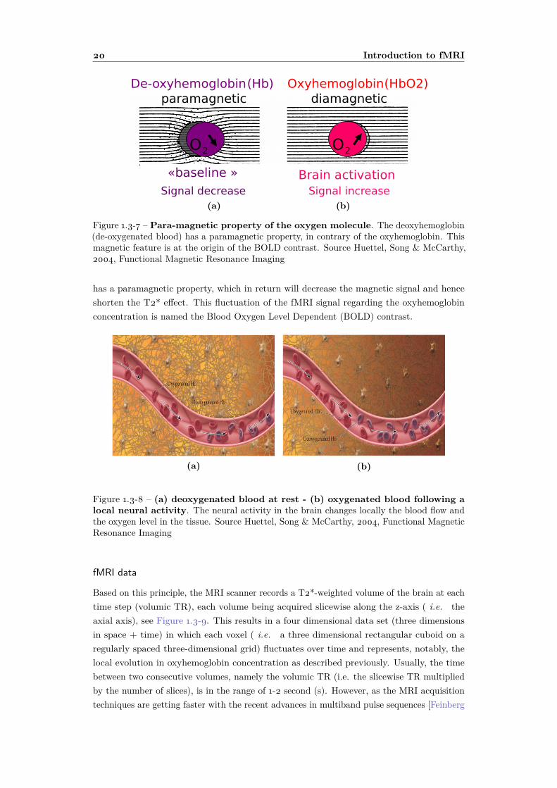
The main mechanism that underlies the fMRI technique relies on the fluctuation ofoxygenated blood in the brain tissue. When a group of neurons fires together they willconsume oxygen and glucose. To provide a continuous supply, the astrocytes, see Figure 1.1-2,will regulate the blood flow to ensure that oxygenated blood irrigates the tissue. Thisvasodilation mechanism is the ground of the fMRI imaging technique. Upon activation,oxygen is extracted by the cells, thereby increasing the level of deoxyhaemoglobin in theblood. This is compensated for by an increase in blood flow in the vicinity of the active cells,leading to a net increase in oxyhaemoglobin, see Figure 1.3-8. This mechanism induces localB0 inhomogeneities. As reported in Figure 1.3-7, the oxyhemoglobin (oxygenated blood) hasa diamagnetic property which will produce an increase of the magnetic signal during the echotime and hence a longer T2* relaxation parameter. On the contrary, the deoxyhemoglobin

2FLuid Attenuated Inversion Recovery pulse sequence that is used to suppress the bright signal in the

CSF as this is a T2 sequence.


O2 O2

Brain activationSignal increase

«baseline »Signal decrease

De-oxyhemoglobin (Hb)paramagnetic

Oxyhemoglobin (HbO2)diamagnetic

(a) (b)

Figure 1.3-7 – Para-magnetic property of the oxygen molecule. The deoxyhemoglobin(de-oxygenated blood) has a paramagnetic property, in contrary of the oxyhemoglobin. Thismagnetic feature is at the origin of the BOLD contrast. Source Huettel, Song & McCarthy,2004, Functional Magnetic Resonance Imaging

has a paramagnetic property, which in return will decrease the magnetic signal and henceshorten the T2* effect. This fluctuation of the fMRI signal regarding the oxyhemoglobinconcentration is named the Blood Oxygen Level Dependent (BOLD) contrast.

(a) (b)

Figure 1.3-8 – (a) deoxygenated blood at rest - (b) oxygenated blood following alocal neural activity. The neural activity in the brain changes locally the blood flow andthe oxygen level in the tissue. Source Huettel, Song & McCarthy, 2004, Functional MagneticResonance Imaging

fMRI data

Based on this principle, the MRI scanner records a T2*-weighted volume of the brain at eachtime step (volumic TR), each volume being acquired slicewise along the z-axis ( i.e. theaxial axis), see Figure 1.3-9. This results in a four dimensional data set (three dimensionsin space + time) in which each voxel ( i.e. a three dimensional rectangular cuboid on aregularly spaced three-dimensional grid) fluctuates over time and represents, notably, thelocal evolution in oxyhemoglobin concentration as described previously. Usually, the timebetween two consecutive volumes, namely the volumic TR (i.e. the slicewise TR multipliedby the number of slices), is in the range of 1-2 second (s). However, as the MRI acquisitiontechniques are getting faster with the recent advances in multiband pulse sequences [Feinberg

1.3. Introduction fMRI 21

et al., 2010, Smitha et al., 2018], they permit lower TR and thus improved temporal resolution.Recent large fMRI data sets such as the Human Connectome Project (HCP) [Van Essenet al., 2013] exhibit TR lower than a second to explore higher frequencies in the BOLD signal,be less prone to physiological artifacts such as heart beat and breathing and potentiallycapture oscillatory neural dynamics (in the delta band) which play an important role inthe coordination of large-scale brain networks [Lewis et al., 2016]. In regards to the spatialresolution in fMRI, the voxel dimension ranges from 1 to 3mm along each axis. Of course,a gain in spatial resolution may be achieved at the expense of a lower temporal resolutiondue to the traditional trade-off between the two. Improved spatial resolution may help finelydelineate cortical activation as far as the sensitivity of detection is maintained, which inturn requires a good temporal SNR. The temporal SNR (tSNR) is thus a key property infMRI [Triantafyllou et al., 2005], defined voxelwise as the ratio of the average signal acrossvolumes divided by the corresponding standard deviation.

Figure 1.3-9 – Illustration of the fourdimensions in fMRI. During an fMRIacquisition, consecutive brain volumes arecollected at a predefined pace defined atthe volumic TR. Source nilearn.github.io

1.3.2 Classical fMRI preprocessing

In this subsection, we describe the classical pipeline to perform the spatio-temporal pre-processing of fMRI data. Indeed, nuisance signals and artifacts may corrupt the BOLDsignal during acquisition. Firstly, the brain scans are not perfectly aligned one another andthus should be spatially re-aligned. Secondly, the subject may move in the scanner duringacquisition, which should be compensated for. Thirdly, all slices in a given volume are notcollected simultaneously, indeed, each slice takes approximately 30 to 40ms to be acquireddepending on the selected spatial encoding scheme (e.g. echo planar imaging combined withparallel imaging). This leads to a significant delay between the first and last slices that mustbe compensated for to permit further statistical analysis in which all voxels are supposedto be collected at the same time point (see Chapter 2). Most often, to meet the timingconstraints of one volume every 1-2s., a high-speed single shot Echo Planar Imaging (EPI)readout is used to collect fMRI data slicewise. Consequently, the data are prone to local B0

inhomogeneities and thus to off-resonance effects, which introduce geometric distortions andsignal drop out in fMRI data, especially in voxels located at the interfaces between air andtissues (e.g. nasal cavities, ear canal). To compensate for this kind of artifacts, the mostpopular strategy in fMRI is called topup [Jenkinson et al., 2012] and consists in collectingtwice the data corresponding to the same slice, first in the top left/bottom right direction inthe 2D k-space plane and second in the opposite direction (bottom right/top left). By doingso, the local B0 inhomogeneities accumulated along the readout axis (left/right) are canceledout. However, this doubles the acquisition time.

The obtained fMRI data could be then registered either to structural MRI data toperform intra-subject normalization or to a brain template to have a spatially coherent basis


to perform comparison with multiple subjects. Moreover, to maximize region overlap betweensubjects, fMRI data are usually convolved with a three-dimensional Gaussian, resulting inspatial smoothing of the data. Finally, the nuisance artifacts that could still be present inthe data, could be estimated for future removal (confound regressors estimation).To summarize the classical preprocessing steps are:

• Alignment : Adjust for movement between scans.

• Head-motion estimation: Correct for movement from the subject.

• Slice-timing correction: Correct for delays between slices.

• Susceptibility distortion: Correct for the presence of artifact (geometric distortionsand signal loss) due to B0 inhomogeneities.

• Coregistration : Overlay structural and functional images.

• Normalisation : Wrap images to fit to a standard template brain for statistical groupanalyses.

• Smoothing : Increase signal-to-noise ratio and maximize between-subject overlap ofactivations.

• Confound estimation : Estimate the nuisance regressors for future removal.

1.3.3 fMRI acquisition

In this subsection, we briefly describe the different types of acquisition that are currentlyused in fMRI to map cognitive functions and investigate ongoing fluctuations of brain activity.To this endeavour, we will introduce first task-related fMRI (tfMRI) acquisitions and secondresting-state fMRI (rs-fMRI) acquisitions and describe the specificity of each imaging session.

Task fMRI acquisition

Task fMRI (tfMRI) is used when the participant is engaged in an experimental paradigm (EP)during the imaging session. This means that the subject is submitted to some specific stimulior is asked to perform certain tasks while his brain activity is recorded at regular intervals.resting periods are introduced between stimuli. The stimuli may be grouped in blocks ofapproximately 30s (block designs) or instead submitted to the subject in a sparse way (event-related designs). In the last scenario, the distance in time between consecutive stimulidetermines whether the paradigm is slow (15 to 20s) or fast event-related (3s). Blockdesigns are known to generate maximal contrast-to-noise ratio (CNR) and thus ease thedetection of evoked activity. In contrast, event-related designs may be useful to estimate thehaemodynamic response function (see chapter 2). Fast event-related designs are particularlyappealing when mixing different types of stimulus (i.e. different experimental conditions) asthey permit to increase the pace between consecutive stimuli and thus preserve a reasonableCNR compared to their slower counterpart.

The nature of the task submitted to the participant varies depending on the purpose ofinvestigation. A simple example is the characterisation of the motor cortex, the correspondingEP for this imaging session could be the finger tapping in which the participant alternates

1.4. Neurovascular coupling in fMRI 23

between rest period and finger tapping. Such acquisition permits to activate the motorcortex and, with an adapted estimation procedure, to determine the precise localization ofthe subject’s brain regions involved in task performance.

Numerous tasks can be submitted to the participant during the imaging session, fromlistening to specific sound patterns to performing a challenging working memory task (e.g.n-back task). The first main objectives of the tfMRI are to spatially localize the subject’sbrain activity in response to these external stimuli. This is easily achieved using blockdesigns. However, when we are interested in the rich fluctuations of the BOLD signal totry to uncover some neural signature in response to some specific stimuli (e.g. priming orrepetition suppression effect), event-related designs are very useful.

This kind of imaging paradigm allows a better understanding of the brain function.However, as each paradigm is focused on a specific cognitive function and because the timespent in the MRI scanner is limited, the analysis of fMRI data provides a limited view onthe global functioning of the brain.

Resting-state fMRI acquisition

Rs-fMRI is the type of acquisition where the participant is not engaged in an experimentalparadigm but instead stays still in the scanner, either keeping his eyes open or closed. Thegeneral idea is to record the nominal and awaken brain functioning to better understand itsglobal functional structure.

Importantly, rs-fMRI reveals functionally connected regions, see Figure 1.3-10, thatare organized into reproducible, well-known and large-scale functional brain resting-statenetworks (RSNs), for examples : default mode network (DMN), attention network, executivecontrol network (ECN), visual network, motor network. Alterations in these RSNs arethought to precede symptoms and structural changes in neurodegeneration by several years,and might allow the identification and quantification of preclinical disease stages.

1.4 Neurovascular coupling in fMRI

In the previous section we highlight the dependence of the fMRI signal on the oxygenationlevel of the blood, yielding to an indirect observation of the neural activity. In this section,we focus on the mechanism between neural activation and an observable change in the BOLDsignal. Then we will detail how useful the estimation of this coupling can be in a clinicalcontext.

1.4.1 Introduction to the neurovascular coupling and its modeling

The neurovascular coupling relies on multiple actors, from the astrocyte cells to smooth musclecells notably. The principle aspect of the response is the vasodilation of the surroundingblood vessels. Once a group of neurons fire together, the glial cells will dilate blood vessels tosupply the neurons in oxygen. As explained previously, this re-oxygenation is then capturedby the MRI scanner through an increased T2∗ decay which produces the BOLD contrast.

A major difficulty related to the BOLD signal is that this oxygenation supply happens acouple of seconds after the neural firing. If we consider a single spike as a proxy for neural


Figure 1.3-10 – Illustration of the rs-fMRI analysis. Identification of the voxels timelycorrelated to estimate the functional networks present in the brain. Source M. P. van denHeuvel and H. E. Hulshoff Pol, Exploring the brain network: A review on resting-state fMRIfunctional connectivity.

activity, the BOLD signal will peak in average 5s later and then return to its baseline afterapproximately 20 to30s seconds.

In order to perform analysis on the BOLD data, this neurovascular coupling was modelas a transfer function which takes as input the neural activation signal and output theBOLD signal. This function was described through a differential equation system and canbe summarized by its Green function. The latter represents the noise-free response of theneurovascular system to a spike input, which could model a very brief neural activation,see Figure 1.4-11. This response is named the Haemodynamic Response Function (HRF).Numerous models have been proposed to encode the HRF shape in various ways but themost common is the double Gamma distribution model introduced in Friston et al. [1998a],see Equation 1.8 where c, α1, α2, β1, β2 are fixed scalars defined by the authors as follows:

v(t) = tα1−1βα11 e−β1t

Γ(α1) − c tα2−1βα2

2 e−β2t

Γ(α2) (1.8)

Figure 1.4-11 – Illustration of the HaemodynamicResponse Function (HRF). The yellow line repres-ents the neural activation in time u and the red linerepresents the BOLD response y to this spike input,namely the HRF. Source Huettel, Song & McCarthy,2004, Functional Magnetic Resonance Imaging.

Moreover, to obtain the response y(t) from any neural activity signal denoted u(t), theinput is convolved with the HRF v(t). Indeed, as described in Boynton et al. [1996], theneurovascular coupling exhibits linear and time invariant (LTI) properties and can then be

1.4. Neurovascular coupling in fMRI 25

faithfully described by a convolution operator:

y(t) =∫ T

0

v(τ)u(t− τ)dτ = (v ? u)(t) . (1.9)

Consequently, the following properties hold:

• Multiplicative scaling: if the amplitude of the neural activation signal u(t) is multipliedby a factor λ, then the produced BOLD signal is scaled by λ too: y(λu(t)) = (v ?(λu))(t) = λy(t).

• Additivity: if the neural activation signal is a sum of multiple spikes (ui(t))i, thenthe corresponding BOLD signal is the sum of the responses yi(t) to each signal ui(t):y(∑i ui(t)) = (v ? (

∑i ui)(t) =

∑i yi(t).

• Time shift invariance: if the neural activation signal is shifted in time from a specificdelay ∆t, then the associated BOLD signal y(t) is shifted by ∆t too: y(u(t−∆t)) =(v ? u)(t−∆t) = y(t−∆t).

In the discrete setting, the counterpart of Equation 1.9 reads:

y = v ∗ u with yn =K−1∑i=0

viun−i. (1.10)

However, this formulation does not take any noise component into account. A commonassumption is to consider the noise ε as an auto-regressive noise of order 1 (also denotedas AR(1): ∀n, εn = aεn−1 + νn where a stands for the auto-regressive parameter and ν theinnovation white Gaussian noise of variance σ2), see Equation 1.11 and Figure 1.4-12.

y = v ∗ u+ ε (1.11)

Figure 1.4-12 – Illustration of BOLD signal modeling. The BOLD signal is obtained byconvolving the neural activity signal u (in red) with the Haemodynamic Response Functionv (in blue) and by adding noise ε (in yellow).

1.4.2 Clinical application

In this section, we propose to discuss the opportunity to use the HRF as a biomarker as ameans to investigate brain function in a healthy or a pathological condition.

The Haemodynamic Response Function as a biomarker

As described earlier, the HRF models a complex cascade of events produced notably by theglial cells. A modification that will affect those cells would induce a change in the HRF shape.Thus, the latter may provide a valuable biomarker to identify the regions that are impairedby a neurodegenerative pathology (e.g. Parkinson’s disease), a neurological disorder (e.g.


epilepsy) or specific drugs (e.g. caffeine). Moreover, depending on its precise representation,the HRF could be used to identify the change occurred in the BOLD response, whether itimplies a re-scaling of its magnitude or a longer delay in the vascular coupling.

The Synchropioid project

The analgesic derived from opium (opioid analgesics) are largely used nowadays with notablyan ongoing crisis due to their massive usage in the USA3. A specific example of opioid is thebuprenorphine. The buprenorphine is an opioid used as analgesic for post-surgical pain orneoplasm pain, it is also used to treat opioid use disorder. This molecule produces a variableanalgesic response for each patient along with a tolerance effect which leads to increase thedrug’s dosage to obtain the same analgesic effect. Thanks to the ceiling effect of its µ-agonistactivity, buprenorphine is also used to treat opioid use disorder, with greater safety and lessaddictive potential than methadone. Such medication induces a patient-dependent analgesiceffect and various degrees of addiction. The reason for this variability has remained unknownso far. To uncover the variability sources and potential addiction factors, the Synchropioïdproject has been set up by the Service Hospitalier Frederic Joliot since 2018 to investigateand characterize the mechanisms of action of the opioid drugs, see Figure 1.4-13. The studywas approved by the biomedical research ethics committee in decembre 2017 (Etude CEA100- 040; EudraCT 2017-001897-41; CPP 2017-12-02-ter).

EFFET

Plasmatic kinetics

Cerebral kinetics

Dose Receptor occupation

Neural activity

Analgesic effect

Analgesic effect

Drug

Figure 1.4-13 – Illustration of the different steps from the injection to the analgesiceffect of the buprenorphine.. The main steps from the injection of the painkiller to theanalgesic effect on the patient. The Synchropioïd project aims to investigate the receptoroccupation step as well as the neural activity step to better characterize the effect of thebuprenorphine on the neurovascular coupling in the brain along with the neural activity.

More precisely, the project aims to characterize the action of the buprenorphine spatiallyand temporally. Buprenorphine is classified as a partial agonist. It has a high affinity, butlow efficacy at the µ-receptor where it yields a partial effect upon binding. It also, however,possesses κ-receptor antagonist activity making it useful not only as an analgesic, but also inopioid abuse deterrence, detoxification, and maintenance therapies. The objective is to forma cohort of 60 subjects (healthy volunteers with no history of substance abuse or addiction)who will receive a dose of the pain killer while being scanned in a with a fully integrated3T PET/MR system (GE SIGNA PET/MR scanner)4. This is a hybrid scanner that allowssimultaneous PET and MR scans for patients, see the photo Figure 1.4-14. This noveltype of machines allows for the precise recording of the localization of the painkiller in thebrain using the PET modality while recording the ongoing fluctuations of the BOLD signal

3https://www.theguardian.com/us-news/opioids4At the time of this manuscript is written, the cohort is not yet fully recruited and the project will be

continuing beyond this PhD thesis.

1.5. Chapter conclusion 27

using the MRI system during resting-state acquisitions. Half of the participants, defined ina randomized controlled trial, will receive a placebo dose (control group) while the otherhalf will receive an analgesic dose (0.2 mg intravenously injected) in order to exhibit thebuprenorphine effect by contrasting the two populations and making statistical comparisons,as done in clinical trials. The group-comparison of the HRF estimates will permit to uncoverin the brain which regions show analgesic-related changes. The general idea here is to usethe HRF as a biomarker to investigate the analgesic effect of opioid and open new avenues ofresearch to better control its effects on patients.

Figure 1.4-14 – PET MR scanner. Photo of the PET MRscanner presents at the Service Hospitalier Frederic Joliotinvolved in the Synchropioid protocol.

1.5 Chapter conclusion

We have introduced the background in neuroimaging, through the description of the brainstructure and function and the various neuroimaging techniques used to investigate them.We have paid attention to the fMRI acquisition setup and described the neurovascularcoupling involved in the origin of the BOLD signal. We have presented the main assumptionsunderlying this coupling, basically summarized by the impulse response of a linear and timeinvariant system also called the Haemodynamic Response Function (HRF). Additionally, wehave emphasized how its estimation is relevant to investigate brain activity in a healthy ordisease condition. In the following, we will describe how to estimate the HRF from fMRIdata and we will introduce novel and efficient methods to that aim.

] ] ]

] ]

]

Chapter 2

How to segregate the vascular and

neuronal components in fMRI?

Chapter Outline

2.1 Introduction to the General Linear Model (GLM) . . . . . . . . . . 292.2 HRF estimation with fixed neural activity . . . . . . . . . . . . . 31

2.2.1 HRF modelling . . . . . . . . . . . . . . . . . . . . 322.2.2 Fitting the HRF model to the observed fMRI data . . . . . . . 33

2.3 Neural activity estimation with fixed HRF . . . . . . . . . . . . . 342.4 Joint estimation of the neural activity and the neurovascular coupling from

BOLD signal . . . . . . . . . . . . . . . . . . . . . . . . 372.5 Conclusion . . . . . . . . . . . . . . . . . . . . . . . . 38

T his chapter introduces state-of-the-art approaches to disentangle the neurovascularcoupling from fMRI data. First, we will detail the General Linear Model (GLM) as it is

the most common method used to identify the brain activity that correlates to a specifictask during the imaging session. Then, we will present the main approaches that havebeen proposed in the literature to estimate the HRF from fMRI data collected during taskperformance, i.e. along the course of an experimental paradigm. In the third section, we willintroduce methods that estimate the neural activation signals from the observed signal witha fixed HRF. Finally, we will introduce the most recent methods that allow for a semi-blind

deconvolution of neural activity from an unknown HRF in a paradigm-free setting, meaningthat the knowledge of the experimental paradigm is no longer required to conduct this kindof analysis and hence such approaches may apply to both task-related and resting-state fMRIdata.

2.1 Introduction to the General Linear Model (GLM)

In this section, we introduce the General Linear Model (GLM) approach. This model de-scribes the observed task-related fMRI (tfMRI) data with a linear combination of predefinedregressors (i.e. temporal atoms) based of the different experimental conditions performedby the participant during the imaging session. The original GLM formulation does not

29

30 How to segregate the vascular and neuronal components in fMRI?

= +

Figure 2.1-1 – General Linear Model illustration. The observed BOLD signal yj isdescribed as the linear combination such as Xβj with the addition of an auto-correlatednoise [Woolrich et al., 2001] denoted εj , which is usually model as an autoregressive processof order 1. Note that the components of X follow the LTI model such as Xk = v ∗ uk withuk being the temporal signature of each conditions.

allow for the estimation of either the HRF or the underlying neural activity signal, howeveras it is the most common method used to perform the analysis of tfMRI, we describe it briefly.

The GLM proposes a massively univariate description of the tfMRI data Y ∈ RT×P .The model makes the hypothesis that voxel’s temporal signal can be recomposed as alinear combination of K predefined temporal components of length T . Each componentis described by the temporal signature of a specific task (condition) of the experimentalparadigm (EP). This signature is convolved with a canonical HRF v that has a fixed andconstant shape for the whole brain to better explained the observed signal. All these temporalsignatures form the design matrix X ∈ RT×K of the experiment, such as X = (Xk)Kk=1 with∀k ∈ [1..K] Xk = v ∗uk with uk ∈ RT describing the temporal onsets of the kth condition.The GLM model is summarized in Equation 2.2 (see also Figure 2.1-1).

For one voxel:

yj =Xβj + εj , (2.1)

with ε ∼ N (0,V )

For P voxels:

Y =Xβ +E, (2.2)

with Y = (yj)Pj=1,β = (βj)Pj=1 and E = (εj)Pj=1

such that ∀j ∈ {1...P} εj ∼ N (0,V ).

Most of approaches propose to minimize a simple quadratic loss as a cost-functionto fit the model parameters to the observed tfMRI data. However, the quadratic loss iswell suited only with the assumption that the noise is Gaussian. As shown by Woolrichet al. [2001], the noise in fMRI is best modelled by a first-order autoregressive process. In

2.2. HRF estimation with fixed neural activity 31

order to remove the correlation in the noise, the most common solution is to apply a priorwhitening on the observed data Y . The correlated noise is given by ε ∼ N (0,V ) whereV ∈ RT×T is the symmetric correlation matrix and σ the standard deviation of the noise.The Cholesky decomposition can be used to find a matrix Q such that V = (Q>Q)−1. Oneapproach to estimate V is to fit a first GLM on the observed data and consider the residualE = Y −Xβ. Then, we fit, on E, a weighted sum of predefined correlation matrices to thisresidual to estimate V [Bollmann et al., 2018]. Thus, the GLM decomposition is used onthe prewhitening problem as :

QY = QXβ +Qε, (2.3)

with Qε ∼ N (0, σ2I).

As β belongs to RK×P , each row βk ∈ RP is a spatial map that encodes which voxelshas a signal that is mostly correlated with the kth experimental condition. Indeed, thecomputation of a T-statistics based on the vector βk allows us to identify the most significantentries which in return permit to localize the most activated voxels in response to thestimulation (e.g. listen to sounds, music or read sentences) associated with the kth condition.

The GLM is impeded by several limitations. First, the haemodynamic response is crudelymodeled for the whole brain. Indeed, despite enhancements proposed by more elaboratedformulations that allow to adapt to some degree the HRF, the GLM assumes a fixed andcommon neurovascular coupling for the whole brain. This assumption is known to be falseand thus makes the standard GLM approach too crude to accurately model fMRI data.Moreover, the LTI model used in the GLM supposes that the conditions ((uk)Kk=1) are usedas a proxy for the neural activity. However, this hypothesis does not take into accountthe possible delays in the participant’s responses during task performance. Second, thesimplistic block or Dirac modelling for a stimulus or an action can depart from the trueneural activation signal as this one should be continuous, in particular in time. Overall, theoversimplistic description of the neural activity impedes the precise modeling of the BOLDfMRI data.

To cope with these issues, numerous contributions proposed to improve the estimation ofthe HRF to better explain the observed data. We will detail these contributions in the nextsection.

2.2 HRF estimation with fixed neural activity

In this section, we detail the most common modelling for the HRF and describe howto estimate the corresponding model parameters from the observed fMRI data. All thecontributions discussed here [Friston et al., 1998a, Aguirre et al., 1998, Friston et al., 1999b,Dale, 1999, Glover, 1999, Goutte et al., 2000, Ciuciu et al., 2003, Casanova et al., 2008,Khalidov and Unser, 2006, Lindquist and Wager, 2007, Vakorin et al., 2007, Lindquist et al.,2009, Khalidov et al., 2011, Pedregosa et al., 2015, Zhang et al., 2013] were proposed intask-related fMRI context where an Experimental Paradigm (EP) is available as a proxy tothe neural activity signal, following the LTI model described in the previous section.


2.2.1 HRF modelling

Most of those contributions to estimate the HRF rely on a few HRF models. With thesame HRF model, the estimation process can vary by making the regularization of the HRFevolve to better capture the true haemodynamic response in a given subject. The mainchallenge with HRF modeling is to find an efficient trade-off between a flexible model that isable to precisely capture the true haemodynamic response in each brain area (reducing theestimation bias) and a reliable model that limits the overfitting by reducing the number ofdegrees of freedom (diminishing the estimation variance). In this subsection, we propose tolist and detail the main HRF models available in the literature.

The Finite Impulse Response (FIR) model. The FIR model [Dale, 1999, Glover,1999] does not assume any particular shape for the HRF which makes it very flexible butprone to data overfitting in the presence of noise. Regularization has thus been introduced toconstrain the overall HRF shape in FIR models, for instance by penalizing the second-orderderivative to end up with physiologically plausible smooth HRF estimates [Goutte et al.,2000, Ciuciu et al., 2003, Casanova et al., 2008].

The linear combination of predefined atoms. Alternatively, to limit the number ofparameters in the model, the HRF v ∈ Rl has been set as a linear combination of predefinedatoms [Aguirre et al., 1998, Friston et al., 1998a, 1999b], such as v = α>B, with α ∈ RR

being the coefficients of decomposition and B = (br)Rr=1 ∈ RR×l the predefined atoms. Theatoms can then be set in order to span all plausible HRFs and hence better capture theneurovascular coupling.Two widespread sets of predefined atoms are:

• Physiologically informed pattern set: Friston et al. [1998a] propose to consider thecanonical HRF (the double Gamma distribution model) and its derivatives in time andwith respect to the dispersion parameter. The two last aforementioned atoms allows toexpress a potentially delayed (i.e. slower or shorter) and sustained (wider HRF peak)neurovascular coupling that better fits the observed data. Note that, based on thisdouble Gamma distribution function some models are limited to the first two atoms,nevertheless the number of atoms are usually set to three. Note that, each of theseatoms can’t be expressed as a linear combination of the others, however this set doesnot strictly define an orthogonal basis.

• B-splines: (or basis spline) is a basis defined from spline functions. A spline is afunction that has minimal support with respect to a given degree, smoothness, anddomain partition. In these approaches [Vakorin et al., 2007, Zhang et al., 2013], theHRF is defined as a linear combination of splines. In Vakorin et al. [2007] the authorspropose to penalize the `2-norm of the first-order derivative of the splines to obtain asmooth HRF estimate.

Other alternatives exist in the literature, such as Khalidov and Unser [2006] and Khalidovet al. [2011] who use wavelets designed to encode the HRF and estimate the neural activity.This example is detailed in the next subsection as a means to estimate the neural activationsignal.

2.2. HRF estimation with fixed neural activity 33

The logit model. To limit model overfitting, parametric HRF models have been proposedas an alternative to complex regularization schemes. Interestingly, the authors of Lindquistand Wager [2007] propose the inverse logit transform and demonstrate its efficiency overmultiple fMRI data sets [Lindquist et al., 2009]. The inverse logit function L is definedby ∀x ∈ R L(x) = 1

1+e−x . The proposed model summarizes the HRF with only sevenparameters (two parameters are fixed by the constraint of a finite support):

v(t) = α1L

(t− T1

D1

)+ α2L

(t− T2

D2

)+ α3L

(t− T3

D3

)(2.4)

2.2.2 Fitting the HRF model to the observed fMRI data

In this sub-section, we will detail how to fit the parameters of the HRF model to the observedBOLD data.

As a first approach, some contributions, as in Lindquist et al. [2009], proposes to considerthe neural activity per voxel as known. This hypothesis is plausible if the most correlatedvoxels to a given condition, are identified in the brain and used to estimate the HRF.

However, in the general case, the neural activity per voxel is unknown. One way to copewith this, is to fit a GLM that embedded the HRF modelling. Considering the fMRI datapre-withen, we fit the GLM to the observed fMRI data by minimizing a simple quadraticdata-fidelity term. Although, estimating both the HRF’s parameters and the coefficient βleads to an ill-posed problem. To manage this problem, the authors, in Pedregosa et al. [2015],propose to introduce a low-rank hypothesis to the GLM, by minimizing the cost-functiondefined in :

arg minαj ,βj ,cj

12‖yj −XBvec(αjβ>j )−Xccj‖22 (2.5)

subject to ‖α>j B‖∞ = 1 and 〈αj ,αref〉 > 0

Here, yj ∈ RT refers to the BOLD signal for one voxel. The nuisance phenomenon aremodeled with Xccj where Xc refers to predefined nuisance regressors with their associatedcoefficients cj . The signal of interest is captured by the term XBvec(αjβ>j ). The designmatrixXB ∈ RT×RK is defined by successively stacking the regressors obtained by convolvingeach of the basis elements with the stimulus onsets of each condition – similarly to the usualdesign matrix used in the GLM models. αj refers to the parameters of the HRF, for onevoxel, modeled w.r.t a set of predefined atoms B = (br)Rr=1 ∈ RR×l such as vj = α>j B.These parameters αj are constrained with the `∞-norm to avoid amplitude indeterminacyand constrained to have a positive scalar product with fixed user-defined reference HRFparameters αref to prevent too large deviations from expected HRF shapes. Finally, the βjdenotes the regressor coefficients for the model.

In this work, the authors rely on the assumption that a linear combination of predefinedatoms B for the HRF, such as v = α>j B and enforce a rank-1 constraint on the coefficientαj for the considered voxel such as vec(αjβ>j ) = [αjβj1,αjβj2, ...,αjβjK ] ∈ RRK×1. Bydoing so, the authors provide a method to estimate one HRF per voxel while identifying themost correlated voxel to each EP in the design matrix.


In this section, we have introduced most common models for the HRF and how theirparameters are estimated from the observed BOLD data. In the following section we will seehow to estimate the neural activity with a fixed and constant neurovascular coupling for thewhole brain.

2.3 Neural activity estimation with fixed HRF

In this section, we give an overview of the different methods proposed to estimate the neuralactivity signals in the brain from fMRI data. Importantly, we will detail the fundamentalwork [Karahanoğlu et al., 2013] that proposed a block signal modelling for the neural activity.This hypothesis is critical for our contributions presented in the next chapters.

We introduce the Toeplitz matrix such that ∀u ∈ RT−L+1 Hvu = v ∗ u. One canestimate the neural activity signal u by minimizing a simple quadratic data-fidelity term as :

arg minu∈RT−L+1

12‖Y −Hvu‖22 (2.6)

SinceHv is not invertible, Equation 2.6 admits multiple minimizer. In order to reduce thevariance of estimation, one can introduce modelling hypothesis on u to make the estimationproblem better conditioned. The neural activity signal models the activity of approximately105 neurons over time during a TR. If we normalize the signal to 1, we can interpret its valueas the proportion of firing neurons among the population belonging to a voxel. A reasonablehypothesis would be to have a smooth evolution of this percentage over time. However, in aBOLD deconvolution context, a flexible smoothness regularization is not sufficient to achieverobust estimation of the neural activity as the overall problem stays ill-posed.

Agnostic neural activation signals modelling. In Glover [1999], the authors proposeto obtain a proxy for the HRF by taking the observed BOLD response of an event-relatedcondition. Indeed, as the HRF is the response of the neurovascular coupling to a Diracinput (impulse event), a direct observation of the BOLD signal after an event will give anoisy observation of the HRF. With this proxy, they propose to estimate the neural activitysignals, denoted u(t) using the Wiener filter :

u(t) = F−1

(H∗(ω)M(ω)

|H(ω)|2 + |N(ω)|2

)(2.7)

with ∗ the complex conjugate, H(ω) the Fourier transform of the HRF, M(ω) the Fouriertransform of the observed BOLD data and N(ω) the Fourier transform of the noise in theobserved data.

This contribution is of special interest since it does not impose any model on the neuralactivity signal. However, the described estimation process can only be applied to even-relatedtask fMRI data for which an estimate of the HRF can be derived beforehand. Moreover, toperform Wiener filtering, one needs to estimate the term |N(ω)|2. These two limitationsreduce the applicability of this approach.

Sparse hypothesis for the neural activation signals. An attempt to improve regular-ization of the neural activity model is to consider that the signal is sparse. In other words, weconsider that most of the coefficients of the 1D vector modelling the neural signal are zeros.

2.3. Neural activity estimation with fixed HRF 35

Doing so, the neural activity is summarized into a few time-locked temporal activationsnamed events.

In Khalidov and Unser [2006], Khalidov et al. [2011] the authors propose to estimatethe neural activation signal by computing it as an output of the Activelet transform of theobserved BOLD data. These wavelets form a dictionary in which the canonical HRF issparsely represented. The neural activity signal is estimated by enforcing sparsity to find themost parsimonious representation for the observed BOLD signal through the minimizationof a LASSO problem.

In Caballero-Gaudes et al. [2011, 2012, 2013] the authors introduce their “paradigm-freemapping” with which they estimate the neural activation signal by regularizing it notablywith the `1-norm in order to recover a parsimonious activation.

Numerous others approaches propose to estimate the neural activity from the BOLDsignal under this sparse hypothesis by introducing a Bayesian framework [Ciuciu et al., 2010,Chaari et al., 2012, Bakhous et al., 2012]. As the remaining of the manuscript focuseson variational approaches, we do not detail those approaches here. Moreover, this sparsehypothesis is known to poorly capture the true neural activity. Representing neural activityas a piecewise constant or block signal has been introduced later on in Karahanoğlu et al.[2013] to improve its representation

Piecewise constant or block signal hypothesis for the neural activation signals.To the best of our knowledge, the first contribution that has introduced this block signalhypothesis in the estimation of the neural activity signal is Karahanoğlu et al. [2013].

• Deconvolution with the Total Variation regularization. In Karahanoğlu et al. [2013]framework, the authors impose sparsity of the first-order derivative of the estim-ated neural activity signal which estimates a piecewise-constant signal, as describedin Equation 2.8 and illustrated in Figure 2.3-2. This regularization involves a TotalVariation (TV) term which will be detailed later on in subsection 3.1.2. Note thatthese authors also impose a spatial smoothness within predefined regions of interestconcerning the denoised BOLD signal.

arg minX∈RP×T

12‖Y −X‖

2F +RT (X) +RS(X) (2.8)

with RT (X) =P∑j=1

λ1j

T∑t=1

|(∆L(Xp,:)):,t|

and with RS(X) =T∑t=1

λ2t‖ ∆Lap(X:,t)‖2,1

with, as previously, P the number of voxels, T the number of scans, Y ∈ RP×T theobserved BOLD signal and X ∈ RP×T the denoised BOLD signal. ∆L = ∆D ◦∆h isthe operator that transforms the BOLD signal into the first order derivative of theneural activity signal, by first applying the HRF deconvolution operator and then thediscrete differential operator, and finally ∆Lap is the Laplacian operator in 3D.

The considered optimization problem is convex inX and minimized with an alternatingoptimization with a Generalized Forward Backward algorithm [Raguet et al., 2013].


Figure 2.3-2 – Scheme of the alternated minimization procedure described in Karahanoğluet al. [2013] to estimate the neural activity ∆h(Xp,:) from the observed BOLD data Y . Theauthors propose to estimate it by introducing notably the block signal hypothesis on theneural activity signal ∆h(Xp,:).

The block signal hypothesis is particularly relevant for task fMRI data collected alongan experimental paradigm with a block design structure as the neural activity signalsmay follow the same pattern. However, this model makes sense as well in the contextof resting-state fMRI data as a means to regularize the spontaneous neural activity.

• Deconvolution with the LASSO. In Costantini et al. [2018] the authors propose toestimate the neural activation signal by fitting a linear model with a quadratic term andand a `1-norm regularization term. They minimize the convex cost-function defined by:

arg minz∈RT

12P ‖Y −HvLz‖22 + λ‖z‖1 (2.9)

with P the number of voxels, Hv the Toeplitz matrix associated with the predefinedand fixed HRF, and L the discrete integration operator. They propose to minimizeEquation 2.9 with the Least Angle RegreSsion (LARS) algorithm for fast estimation.

While this method might appear as modeling the neural activity as a sparse signal, it isin fact the synthesis formulation for a block model. Indeed, as z is sparse, the recoveredsignal Lz obtained with the integration operator L has a piece-wise constant structure.While this formulation leads to a simpler optimization procedure, it is usually sloweras we show in chapter 4.

In this section, we have described the most common neural activity signal modelingalong with their estimation method from the observed BOLD signal. However, as theseapproaches rely on a constant and fixed HRF shape to deconvolve the observed signal, theyalso introduce a bias w.r.t the neurovascular coupling. In the following section, we willpresent recent contributions that aim to estimate both the HRF and the neural activity inan attempt to remove this bias.

2.4. Joint estimation of the neural activity and the neurovascular couplingfrom BOLD signal 37

2.4 Joint estimation of the neural activity and the neurovascular

coupling from BOLD signal

A natural question would be to know if one can estimate these two components jointly fromfMRI data. Since we aim at estimating the neural activity without an explicit knowledgeof the HRF, one may refers to this problem as the blind deconvolution. In our case, as weconstrain the structure of the HRF by using a limited set of parameters, we refer to thisproblem as the semi-blind deconvolution. We next describe some interesting attempts tosolve this problem.

As previously introduced, the two main assumptions that dominate the neural activitysignal modeling are the sparse signal and the block signal hypothesis. We propose to detailrecent contributions in both case in the perspective of blind deconvolution.

Sparse hypothesis for the neural activation signals. In Wu et al. [2013] the authorspropose to estimate the most prominent peaks in the observed BOLD signal by retainingonly the entries that exceed a certain threshold. With this summary of the fMRI data, theyestimate the haemodynamic delay. Then, they fit the HRF parameters (the response height,the Full Width at Half Max (FWHM) of the HRF and its Time to Peak (TP)) to match thisdelay and in return they deconvolve the observed BOLD signal with this estimated HRF, seeFigure 2.4-3 for illustration. Note that this different steps are not repeated, hence, the HRFis not corrected from the estimated neural activity and inversely.

Figure 2.4-3 – Estimation process proposed in Wu et al. [2013]. The BOLD signal issummarized with its most prominent peaks on which the haemodynamic delay is estimated.An HRF is then fitted to correspond to this estimated delay which in return allows todeconvolve the observed BOLD signal.

However, as described in the previous section, the sparse hypothesis poorly captures theneural activity. We once again turn to the block signal hypothesis which allows for a gain inflexibility and thus in estimation performance.

Block signal hypothesis for the neural activation signals. In Farouj et al. [2019] theauthors propose to minimize Equation 2.10 to estimate both the HRF coefficients defined asa linear combination of predefined atoms and estimate the neural activation signal similarlyto Karahanoğlu et al. [2013]. They consider the cost-function defined by :


arg minα∈R2,xj∈RT

12‖yj − xj‖

2F + λ1‖DH−1

α xj‖1 + λ2‖α−αref‖22 (2.10)

with yj ∈ RT the observed BOLD data and xj ∈ RT the estimated denoised BOLD dataand λ1 and λ2 the regularization parameter. The parameters of the model are estimated byminimizing Equation 2.10, using a the generalized forward–backward splitting algorithm, asproposed in Karahanoğlu et al. [2013].

Figure 2.4-4 – Semi-blind deconvolution proposed in Farouj et al. [2019]. The HRF modellingis based on the linear combination of predefined atoms and the neural activity modelcorresponds to the hypothesis of a block signal.

Point process analysis. Interestingly, in Tagliazucchi et al. [2010], the authors proposes .This characterization of the inter-regions interactions leads to recover the HRF for the targetregion and allows the deconvolution of the observed BOLD with the estimation neurovascularcoupling for the region. The noteworthy aspect of this method, is that

2.5 Conclusion

In this chapter, we have progressively introduced methods that estimate (i) the vascularcoupling in the context of task fMRI experiments for a given representation of neural activitythrough the stimulus onsets, then (ii) inversely and finaly (iii) both components in a semi-

blind deconvolution setting. The main limitations of these works have been outlined. Morespecifically, they proceed voxelwise, i.e. in an univariate manner and do not take the spatialstructure into account, whether this structure concerns the vascular coupling or the spread ofneural activity throughout the brain. Including this kind of structure in new methods couldbe a significant step forward to capture both components in a more robust way and makethese novel approaches less prone to data overfitting. Extending the methods presented herethe better account for the multivariate nature of the signal is one of the core contribution ofthis thesis, that we describe in chapter 5 and chapter 6.

] ] ]

] ]

]

Chapter 3

TV problems minimization with iterative

algorithms

Chapter Outline

3.1 Introduction to regularization in optimization . . . . . . . . . . . . 393.1.1 General introduction to regularization . . . . . . . . . . . . 393.1.2 Introduction to the TV regularization . . . . . . . . . . . . 40

3.2 Solving a TV regularized problem . . . . . . . . . . . . . . . . 423.2.1 Analysis formulation . . . . . . . . . . . . . . . . . . 423.2.2 Synthesis formulation . . . . . . . . . . . . . . . . . . 46

3.3 Performance comparison . . . . . . . . . . . . . . . . . . . 473.3.1 Material and methods . . . . . . . . . . . . . . . . . . 473.3.2 Results . . . . . . . . . . . . . . . . . . . . . . . 48

3.4 Chapter conclusion . . . . . . . . . . . . . . . . . . . . . 50

I n the previous chapter, we have introduced the Total Variation regularization (TV-reg) asa means to regularize the neural activation signals and make the global estimation better

conditioned. The purpose of this chapter is to introduce the TV-reg in 1-dimension (1D)in detail. We define and explore the specific characteristics of this regularization, explainhow to minimize a TV regularized problem by introducing several algorithms to that aimand compare their performances experimentally. A theoretical comparison of the differentformulations of the problem is given in chapter 4.

3.1 Introduction to regularization in optimization

3.1.1 General introduction to regularization

In machine learning or signal processing ill-posed problems often appear such as image recon-struction, source localization or classification. In order to make the estimation feasible, onecan introduce a prior to promote solutions that satisfies certain properties. A usual solutionin the Bayesian setting is to provide a specific distribution regarding the parameters toestimate. In a variational context, a solution is to add possibly multiple regularization terms

39

40 TV problems minimization with iterative algorithms

−10 −5 0 5−10.0

−7.5

−5.0

−2.5

0.0

2.5

5.0

7.5

λ = 0.0

−10 −5 0 5−10.0

−7.5

−5.0

−2.5

0.0

2.5

5.0

7.5

λ = 1.0

−10 −5 0 5−10.0

−7.5

−5.0

−2.5

0.0

2.5

5.0

7.5

λ = 10.0

−10 −5 0 5−10.0

−7.5

−5.0

−2.5

0.0

2.5

5.0

7.5

λ = 1000.0

Figure 3.1-1 – Cost-function evolution w.r.t the regularization parameter λ: In thissimplistic example, we display the cost function level set with different level of regularizationλ ∈ {0.0, 1.0, 10.0, 1000.0}. We can notice that the minimum set evolve from an hyperplanof dimension 1 (a straight line) when λ = 0 to a singleton for λ > 0.

in the associated optimization problem. Depending on the nature of the introduced regular-ization, one can add information on the structure of the estimate, its norm, its smoothness, etc.

To give a simple intuition on how additional terms in a cost-function can improve theconditioning of the problem, let’s consider A ∈ Rm×n with m ≤ n and y ∈ Rm. If we tryto find u ∈ Rn such that y ≈ Au, we might consider the following cost-function F definedby L(·) = 1

2‖y −A · ‖22. However, with that simple loss function, we can’t select a unique

solution. Indeed, for any minimizer u and for u0 ∈ Ker[A]\{0}, we have L(u) = L(u+u0).

The problem is said to be ill-posed as there are infinitely many equivalent solutions. Byadding a regularization term, for example here the `2-norm, such that F (·) = L(·) + λ‖ · ‖22,we can distinguish these equivalent solutions. Indeed, while the data-fidelity terms are equalsfor all u + u0, if u is in Ker

[A]⊥, then u has the smallest `2 norm and will be promoted

among all the other equivalent solutions. Thus, the regularization allows to select among allsolutions with equivalent data-fitting term a solution that verifies a certain property – herea small `2 norm. The unicity of the solution is guaranteed here since L is strongly convex.This is illustrated on a simplistic example with y ∈ R2 such as y = [4 0]> and A ∈ R2×2

with rank(A) = 1 such as:

A =[

2 00 0

]

Figure 3.1-1 shows that, if we set λ = 0, the set of minimizers of the cost-function F isthe one dimensional vector space defined by Θ = {u ∈ R2 such as u = [2 a]> with a ∈ R}.However, whenever λ > 0, the solution set reduces to a singleton. Hence, the estimationproblem associated with F is better conditioned. A classical example of regularization isthe `2-norm, `1-norm or the elastic-net [Zou et al., 2004] norm which combines both theprevious ones.

3.1.2 Introduction to the TV regularization

The TV-reg promotes piece-wise constant estimates by penalizing the `1-norm of the firstorder derivative of the estimated signal. If we consider a signal u ∈ Rn, the associated TVregularization is defined by: ‖u‖TV = ‖Du‖1 =

∑ni=2 |ui − ui−1| with D being the discrete

differential operator such as D ∈ R(n−1)×n and defined by:

3.1. Introduction to regularization in optimization 41

D =

−1 1 0 . . . 0

0 −1 1. . .

......

. . . . . . . . . 00 . . . 0 −1 1

As the `1-norm promotes sparsity on the first order derivative, namely z = Du, thispushes z to be a Dirac signal and thus u to be a piece-wise constant signal. Figure 3.1-2displays two examples where we generate sparse signals Du1 and Du2 and integrate themto obtain the piece-wise constant signals u1 and u2.

0 50 100 150 200 250 300

−1.0

−0.5

0.0

0.5

1.0

x1 Dx1

0 50 100 150 200 250 300

−1.0

−0.5

0.0

0.5

1.0

x2 Dx2

Figure 3.1-2 – Examples of two piece-wise constant signals: u1, u2, along with theircorresponding Dirac signals Du1, Du2. The sparsity of Du1 is higher than the one of Du2,i.e. ‖Du1‖0 ≤ ‖Du2‖0

To illustrate the effect of TV-reg, we provide a simple 1D illustration. We considerthe BOLD signal deconvolution problem for a synthetic signal Figure 3.1-3. We generatea time series z with a support S(z) = 6 which we integrate to obtain a block signal u.This signal is then convolved with the canonical HRF [Friston et al., 1998a] and we add aGaussian noise. We estimate the synthetic source signal u by minimizing the cost functionP (u) = 1

2‖y − u ∗ v‖22 + λ‖u‖TV , with λ set manually. In Figure 3.1-3, we can see that we

recover most of the variations of the original signal as the minimization of P deconvolvesand denoises the observed signal.

Finally, we can mention that the TV regularization is a useful tool for a large number ofapplications. For 1D signals, we already mentioned that it has been used in neuro-imaging fordeconvolution problems [Karahanoğlu et al., 2013]. Recent work also used TV-regularisationas a detrending step to preprocess oculo-motor recordings [Lalanne et al., 2020]. Mostapplication of TV-reg are for 2D image processing problems such as denoising [Rudin et al.,1992, Chambolle, 2004, Darbon and Sigelle, 2006], medical image reconstruction [Tian et al.,2011] along with many of other applications [Rodríguez, 2013]. In this chapter, we willconsider only the 1D case to focus on the BOLD deconvolution model that we introducedpreviously.

0 50 100 150 200

−1.5

−1.0

−0.5

0.0

0.5

1.0

Observed signal

Denoised signal

Original source signal

Estimated source signal

Figure 3.1-3 – Synthetic BOLD deconvolution example with the TV regularization:We display the estimation of the source signal in orange from the observed signal in blue

which was obtained by convolving the original source signal with the canonical HRF and byadding a Gaussian noise.


In the previous chapter, we consider the cost-function F (·) = 12‖v ∗ · − y‖22 + ‖D · ‖1.

By introducing the Toeplitz matrix associated to v, we rewrite F such that F (·) = 12‖Hv ·

−y‖22 + ‖D · ‖1. Moreover to generalize the problem we consider A ∈ Rn×m instead ofHv. In this manner, we introduce the TV regularized problem which consists in finding theminimizer of the function P .

minu∈Rm

[P (u) = 1

2‖y −Au‖22 + λ‖Du‖1

], (3.1)

We can make a couple of remark on P . First, it is a proper and closed function whichmeans that P is a lower semicontinious function. Moreover, P is coercive which means thatP admits a minimizer. However, it is also convex since the data fidelity term is a quadraticterm, which means that any local minimum will be a global minimum. However, even thoughf(·) = 1

2‖y −A · ‖22 is a smooth function, the use of the `1-norm in the regularization makes

g(·) = λ‖ · ‖TV not differentiable. In the following section we will see how to minimize Pconsidering those properties.

3.2 Solving a TV regularized problem

In this section, we detail several approaches to solve the TV-reg problem. The formulationproposed in Equation 3.1 is named the analysis formulation. Other equivalent formulationsare also presented as well has the classical algorithms to minimize them efficiently.

3.2.1 Analysis formulation

Solving the analysis formulation by the book

Considering a cost function defined by F = f + g with f : RT → R+ being convex andsmooth and g : RT → R+ being convex, the most straightforward approach to minimize Fis to consider the proximal gradient descent (PGD) [Rockafellar, 1976]. PGD algorithmalternates between two steps during each iteration t. The first is called the gradient step anddecreases the cost-function along the descent direction defined by the gradient ∇f(u(t)), suchthat u(t+1) = u(t) − ρ∇f(u(t)). The step-size ρ can be chosen in [0, 2

L [ with L the Lipschitzconstant of the gradient operator to have theoretical guaranty on the convergence. Thesecond step is the proximal step, where the regularization term g in the cost-function is takeninto account to provide a feasible point by solving at each iteration the proximal operator ofprox(g, ρ)(.). The proximal operator step consists in solving the problem Equation 3.2 w.r.t

the iterate u(t+1).

u(t+1) = arg minu∈Rm

12‖u

(t+1) − u‖22 + g(u) , (3.2)

In some cases, the proximal operator admits a closed-form solution. In the case of the`1-norm, this is the so call soft-thresholding or for a convex set characteristic function, this isthe orthogonal projection on the set. In the case of the TV-reg, the proximal operator stepin Algorithm 1 does not have a closed-form solution. Hence, one needs to solve Equation 3.2numerically with one of the algorithms exposed in the next paragraphs. However, in the 1Dcase, powerful dynamic programming algorithms have been developed to solve it exactly (upto numerical precision), such as the taut-strings algorithm [Condat, 2013a]. Interestingly,

3.2. Solving a TV regularized problem 43

this algorithm has a complexity of O(T)in most practical cases, which allows to efficiently

solve the proximal step in Algorithm 1.Note that the `1-norm can be replace by a smooth function such as the Huber loss in

order to smooth the cost-function. In this case, the function can be minimized with secondorder approaches [Byrd et al., 1995].

If we consider our cost-function P in Equation 3.1, here we have f such as f(u) =12‖y−Au‖22 and ∇f(u(t)) = A>(Au(t)−y); the regularization term g is the aforementioned

TV-reg, such as g(u) = λ‖Du‖1. Hence, for a scaling parameter 1ρ , the proximal oper-

ator prox(g, ρ)(u) is defined by prox(g, ρ)(·) = arg minu∈RT

[12‖u− ·‖22 + λ

ρ‖Du‖1]. The

corresponding PGD algorithm in the analysis formulation is defined in Algorithm 1.

Algorithm 1: Analysis Proximal gradient descentInput :BOLD signal y, ε, ρ

1 initialization: u(0) = 0T, t = 0 ;

2 repeat3 u(t+1) = u(t) − 1

ρA>(Au(t) − y)

4 u(t+1) = arg minu∈RT

[12‖u(t+1) − u‖22 + λ

ρ‖Du‖1]

5 until ‖u(t+1) − u(t)‖2 ≤ ε;

algorithm 1 is guaranteed to converge to a solution of Equation 3.1 when the step size isproperly set as the previously mentioned – as the inverse of the Lipschitz constant of thegradient. Additionally, one can compute at each iteration an optimal decreasing step ρ∗

to have a better descent, with the backtracking line search based on the Armijo-Goldsteincondition [Armijo, 1966] for example. Another way to accelerate the algorithm 1 is tointroduce a momentum term [Nesterov, 2013, Liang and Schönlieb, 2018]. The idea is toconsider the previous update direction u(t) −u(t−1) to update the next iterate u(t+1). To gofurther in the acceleration, a restarting scheme can also be added [Kim and Fessler, 2018],the main objective of those techniques is to cancel the potential rebound of the cost-functionevolution w.r.t the iteration. We will not go into detail but the accelerating and the restartingscheme will be implemented and their performances will be compared with the classical PGDalgorithm in the next section.

Solving the analysis formulation with primal-dual algorithms

Another type of algorithms to solve cost-functions involving a regularization term g is theprimal-dual algorithm. Here the term dual refers to Lagrangian duality. The idea behindsduality is to consider that an optimization problem can be seen in two different ways: adirect minimization of the cost-function or a maximization of a concave lower bound of thiscost-function.

The main benefit of primal-dual algorithms is that both the primal variable u and thedual variable denoted µ, in our case, are updated simultaneously. To that aim, we introduce avariable z and re-write the regularization term as a constrain: our main problem Equation 3.1is equivalent to the minimization problem Equation 3.3.


minu∈Rm

[P (u) = 1

2‖y −Au‖22 + λ‖z‖1

],

subject to Du− z = 0 .

(3.3)

We derive the associated Augmented Lagrangian function L Equation 3.4 from Equa-tion 3.3 to relax the constraint by introducing the dual variable µ ∈ Rm−1

L(u,y, µ) = 12‖y −Au‖

22 + λ‖z‖1 + µ>(Du− z) + γ

2 ‖Du− z‖22 , (3.4)

L is the Augmented Lagrangian and can be minimized via any primal-dual algorithms.Here we provide the example of the Alternating Direction Method of Multipliers (ADMM)introduced in Boyd et al. [2011], see algorithm 2.

Algorithm 2: ADMMInput :BOLD signal y, ε, ρ

1 initialization: u(0) = 0T, z(0) = 0

T−1, µ(0) = 0

T−1, t = 0 ;

2 repeat3 u(t+1) =

(A>A+ ρD>A

)† (A>y −D>µ(t) + ρD>z(t)

)4 ∀i ∈ [1..T ] z

(t+1)i = 1

ρ (µ(t))i + (Du(t+1))i + λγ sign(z(t)

i )5 µ(t+1) = µ(t) + γ

(Du(t+1) − z(t+1)

)6 until ‖Du(t) − z(t)‖2 ≤ ε;

At each iteration we minimize mathcalL w.r.t u, z and then we make a ascent gradientstep concerning µ such as µ(t+1) = µ(t) + γ

(Du(t+1) − z(t+1)

). Note that the update of u

and z can be distributed.

Condat [2013b] proposes an accelerated primal-dual algorithm, by doing a joint gradientdescent in the primal along in the dual. The algorithm and its properties are detailed inCondat [2013b], we simply report the definition of the algorithm here algorithm 3:

Algorithm 3: Condat-VuInput :BOLD signal y, ε, τ , σ, ρ

1 initialization: u(0) = 0T, z(0) = 0

T−1, t = 0 ;

2 repeat3 u(t+1) = u(t) − τA>(Au(t) − y)− τD>z(t)

4 z(t+1) = z(t) + σD(2u(t+1) − u(t))− ST σ(z(t) + σD(2u(t+1) − u(t)))5 u(t+1) = ηu(t+1) + (1− η)u(t)

6 z(t+1) = ηz(t+1) + (1− η)z(t)

7 until ‖Du(t) − z(t)‖2 ≤ ε;

In this section, we have briefly introduce primal-dual algorithms which are based on theconcept of Lagrangian duality. In the next section, we will see that there is another possibledefinition for the dual and we introduce the Fenchel’s duality.

Solving the dual of analysis formulation

The Fenchel’s duality is a generalization of the Lagrangian duality, thus the intuition of theapproach is same. To obtain the associated dual problem, we define the Fenchel’s transform,defined by:


∀u∗ ∈ Rm f∗(u∗) = − infu∈Rm

(f(u)− u∗>u

)(3.5)

Applying this transformation to our cost function gives us the dual formulation of ourproblem, which leads to a problem with a simpler proximal operator associated to the newregularization term. To prove it, we now derive the dual of Equation 3.1. By defining fand g, such as f(·) = 1

2‖A · −y‖22 and g(·) = λ‖ · ‖1 and by denoting p the minimum of

Equation 3.1 w.r.t u, the problem reads:

minu∈Rm

f(u) + g(Du) (3.6)

With the Fenchel-Rockafellar duality theorem, we derive the dual in Equation 3.7.

minµ∈Rm

f∗(−D>µ) + g∗(µ) (3.7)

With µ ∈ Rm being the dual variable, we have g∗(µ) = −minu∈Rm g(u)−µ>u. With acomponent-wise minimization, we obtain g∗(µ)i = δ|µi|≤λ with δ being the convex indicator.Thus, we deduce that g∗(µ) = δ‖µ‖∞≤λ. Then, we have f∗(µ) = −minu∈Rm f(u)− µ>u.By cancelling the gradient we obtain: f∗(µ) = 1

2‖A†>µ‖22 + µ>A†y, with A† being the

pseudo-inverse of A. Note that, if we set A = I, we obtain the same problem as Chambolle[2004], Barbero and Sra [2018].

Finally, we obtain the Fenchel dual of the optimization problem Equation 3.1:

minµ∈Rm−1

12‖A

†>D>µ‖22 − µ>DA†y (3.8)

s.t. ‖µ‖∞ ≤ λ

With Equation 3.8, we can derive a projected gradient descent algorithm easily. Indeedthe proximal operator associated to the constraint term µ→ δ{‖µ‖∞≤λ} is simply a projection

such as Pj(µ)i =µi if |µi| ≤ λ

sign(µi) λ if |µi| > λ

Algorithm 4: Dual Projected gradient descentInput :BOLD signal y, ε

1 initialization: z(0) = 0T, t = 0 ;

2 repeat3 µ(t+1) = µ(t) − 1

ρ ((DA†)(DA†)>µ− y>(DA†))

4 µ(t+1)i =

µ(t+1)i if |µ(t+1)

i | ≤ λ

sign(µ(t+1)i ) λ if |µ(t+1)

i | > λ

5 until ‖(DA†)(DA†)>µ− y>(DA†)‖2 ≤ ε;

As we mention, the proximal operator involved in this algorithm has a closed formsolution and thus is easy to implement. However, the gradient term involved A† the pseudo-inverse of A. Depending on the rank of the observation matrix its pseudo-inverse could beill-conditioned and the Lipschitz constant of the gradient could be too high, thus producinga too small step size to achieve a fast minimization.


3.2.2 Synthesis formulation

Finally, in this subsection we detail that the analysis formulation of Equation 3.1 can berewritten in the so called synthesis formulation. The general idea is to simplify the regulariz-ation term with a change of variable. Suppose that we consider a regularization defined by gsuch as ∀u ∈ Rm g(u) = ‖Mu‖1 with M ∈ Rm×m being invertible. Then, we could definedz = Mu ∈ Rm such as g(u) = ‖z‖1. Note that the proximal operator of the `1-norm isthe Soft-Thresholding operator. Thus, with this change of variable we obtain a closed-formsolution for the proximal operator involved in the PGD algorithm.

However, if we consider our cost-function in Equation 3.1 we have M = D, with Dbeing not invertible. Thus, we should slightly adapt the described scheme in our case. Weintroduce L ∈ RT×T and R ∈ RT×T , such as:

L =

1 0 . . . 0

1 1. . .

......

. . . . . . 01 . . . 1 1

R =

0 0 . . . 0

0 1. . .

......

. . . . . . 00 . . . 0 1

L is the discrete integration operator and R asserts that ∀ z ∈ RT such as u =Lz we have ‖Du‖1 = ‖Rz‖1. Indeed, with R, we regularized all the coefficients of zexcept the first one, which allow recover u with the integration, such as u = Lz, as desired.With this adapted change of variable, we now derive the equivalent synthesis formulation inEquation 3.9:

minz∈RT

[PAL,λ(z) = 1

2‖y −ALz‖22 + λ‖Rz‖1

], (3.9)

With Equation 3.9, we recover the Least Absolute Shrinkage and Selection Operator(LASSO) problem formulation, which involves a quadratic fidelity term and a `1-norm. Wecan now derive easily a PGD algorithm to minimized it, see algorithm 5:

Algorithm 5: Synthesis Proximal gradient descent (LASSO)Input :BOLD signal y, ε, ρ

1 initialization: z(0) = 0T, t = 0 ;

2 repeat3 z(t+1) = z(t) − 1

ρ (AL)>(ALz(t) − y)4 z(t+1) = ST λ(z(t+1))5 until ‖z(t+1) − z(t)‖22 ≤ ε;

This algorithm is also known as the Iterative Soft-Thresholding Algorithm (ISTA) pro-posed by Daubechies et al. [2004]. It can be accelerated using a momentum term, as proposedin Beck and Teboulle [2009] with the algorithm Fast ISTA (FISTA).

Moreover, to minimize the LASSO problem at Equation 3.9, the Least Angle Regression(LARS) algorithm can be used. LARS algorithm includes iteratively the coefficients of zto produce an estimate with the smallest support S = {i|zi 6= 0}. At each iteration k thealgorithm selects the line ALi most correlated with the residual y−ALz(k) and updates thecorresponding coefficient z(k)

i with a gradient step. At iteration l, if another lineALj becomesmore correlated with the residual, the algorithm includes the corresponding coefficient z(l)

j

to the active-set, such as S(l) = {j}⋃S(l−1) = {i, j}, and updates it ( i.e. z

(l)i and z(l)

j )

3.3. Performance comparison 47

with a gradient step. If a coefficient hits 0 the algorithm removes it from the active-set. Thisapproaches continues to include coefficients until all the coefficients have been considered.

The LARS algorithm is similar to stepwise regression approaches that include iterativelycoefficients and minimize exactly the cost-function w.r.t the current active-set. The LARSalgorithm was introduced by Efron et al. [2004] and it was first applied to the case of theLASSO by Harchaoui and Lévy-Leduc [2007].

To recap, in this section, we have listed and detailed most of the different approaches tosolve the TV-reg problem. We have seen that we could derive multiple equivalent formulationof the same problem which produce different algorithms. A natural question would be toinvestigate which algorithm proposes the fastest minimization of our original problem, wewill see this in the next section with an experiment benchmark on synthesis data.

3.3 Performance comparison

To practically explore which algorithms has the best performance we propose to benchmarkeach of them in a simple deconvolution problem as exposed in Cherkaoui et al. [2019a].

3.3.1 Material and methods

We consider a source signal u ∈ RT with T = 100 such as ‖Du‖0 = 5 in a first scenario and‖Du‖0 = 50 in a second scenario. We consider an HRF v ∈ Rl with l = 60 following theHRF model proposed in Cherkaoui et al. [2019a] with the time dilation parameter δ = 1.We introduce the Toeplitz matrix H ∈ RT+l−1×T associated to v. We generate a singlesynthetic BOLD time serie defined as y = v ∗ u + ε such as y ∈ RT+l−1 and ε ∈ RT+l−1

being a Gaussian noise such as the observed signal as a signal to noise ratio (SNR) of 0.0 dB.

To estimate the source signal u from the observed signal y we propose to solve Equa-tion 3.10, defined as:

minu∈RT

[PH,λ(u) = 1

2‖y −Hu‖22 + λ‖Du‖1

], (3.10)

Equation 3.10 is similar to Equation 3.1, the only difference being the observation matrix,since A = H which provide here a specific structure in this observation operator, notethat in this case the matrix is not invertible. Here we fix arbitrary λ = 1.0. In general thesetting of this hyper-parameter is important since it controls the bias of the estimator definedby y → arg minu∈RT [PH,λ] (u). However, since our objective in this section is simply anoptimization performance comparison we will set λ arbitrary.

We choose to benchmark the proximal gradient descent with analysis primal formulation,the Condat-Vu algorithm, the analysis dual formulation, the synthesis primal formulation.We also consider the LARS algorithm with the synthesis primal formulation. We madethe choice to not include the ADMM algorithm 2 since its performances are known to besub-optimal in comparison of the Condat-Vu algorithm 3. Moreover, as it’s know that theaccelerating and restarting scheme can greatly improve the optimization performance of an


PGD algorithm, we include them in the benchmark.

We fix all the step size to the inverse of the Lipschitz constant of the gradient, except forthe Condat-Vu algorithm. For the later, we manually fix σ = 0.5 after a previous benchmarkand set optimaly τ w.r.t σ according to Condat [2013b].

We propose to introduce the momentum acceleration and the restarting scheme to theanalysis primal PDG algorithm and the synthesis primal PDG algorithm. For the analysisformulation, we define the momentum, at iteration t+ 1, as θt+1 = 1

1+√

1+4(θt)2with θ0 = 1

such as at each iteration u(t+1) = u(t+1) + θt−1θt+1 (u(t+1) − u(t)) with u(t) being the output of

the proximal operator step of the iteration; we do similarly for the synthesis formulation w.r.t

z(t). Moreover, concerning the restarting scheme, we reset the momentum such as θt+1 = θt

when PH,λ(u(t+1)) > PH,λ(u(t)); we do similarly for the synthesis formulation.Each algorithm performs 30000 iterations completely and we store at each iteration

the cost-function value PH,λ(u(t)) along with the duration of the iteration without thecost-function computation duration.

To unsure, fair comparison we initialize each algorithm to the same variable, we chooseµ(0)) = 0T−1, by applying the K.K.T conditions we obtain u = (A>A)†(A>y −D>µ)such as u(0) = (A>A)†A>y which correspond to u(0) = A†y and z(0) = Du(0). Thoseequivalent initializations assert that the cost-function evolution starts at the same value foreach algorithm.

A summary of the parameters of the different algorithms can be found in Table 3.1.

3.3.2 Results

We investigate two scenarios, ‖Du‖0 = 5 and ‖Du‖0 = 50 with Du ∈ R99. In Figure 3.3-4and Figure 3.3-5, we report the evolution of the cost-function PH,λ(x(t))− PH,λ(u∗) w.r.t

the iterations t and the time in seconds for each algorithms in log-scale for both scenarios.We exclude the LARS algorithm form the loss comparison but will report later its averageconvergence time.

In both case, we observe that the order of performance for each algorithms stays the same.We notice that only the synthesis primal PGD and APGD did not reach the minimum of thecost-function whereas all the other algorithms have. We observe that the synthesis formulationalgorithms (PGD, APGD, RAPGD) have the worst performance, as a comparison, the fastestsynthesis formulated algorithm (RAPGD) takes 100 more iterations to converge to the samecost-function value than the RAPGD analysis primal formulation. The Condat-Vu algorithmhas in-between performance, yet it has similar performance of the RAPGD synthesis primalformulation algorithm. Moreover, the PGD analysis dual formulation algorithm has one ofthe worst performance. In addition, all the analysis primal formulation algorithms (PGD,APGD, RAPGD) have the best minimization performance, the RAPGD scheme being thefastest algorithm to reach the minimum for both scenarios. The good performance of theanalysis primal formulation algorithm can be explained by the efficiency of the proximaloperator step in comparison of the synthesis formulation.


Table 3.1 – Summary of the algorithm’s hyper-parameters used to benchmark their performance.

Algorithm Step size Momentum Restarting InitializationAnalysis primal

Proximalgradient descent

(Analysis primal PGD)

ρ = ‖H‖F - - u(0) = A†y

Accelerated Analysis primalProximal

gradient descent(Analysis primal APGD)

ρ = ‖H‖Fθt+1 = 1

1+√

1+4(θt)2

u(t+1) = u(t+1) + θt−1θt+1 (u(t+1) − u(t))

a - u(0) = A†y

RestartingAnalysis primal


(Analysis primal RAPGD)

ρ = ‖H‖Fθt+1 = 1

1+√

1+4(θt)2

u(t+1) = u(t+1) + θt−1θt+1 (u(t+1) − u(t))

b if PH,λ(u(t+1)) > PH,λ(u(t))

then θt+1 = θtu(0) = A†y

Condat-Vuσ = 0.5

1τ =

‖H‖F2 + σ‖D‖Fη = 1.0

- -u(0) = A†y

andz(0) = Du(0)

DualProjected

gradient descent(Analysis dual PGD)

ρ = ‖H†D‖F - - v(0) = 0T−1

SynthesisProximal

gradient descent(Synthesis primal PGD)

ρ = ‖HL‖F - - z(0) = DA†y

Accelerated SynthesisProximal

gradient descent(Synthesis primal APGD)

ρ = ‖HL‖Fθt+1 = 1

1+√

1+4(θt)2

z(t+1) = z(t+1) + θt−1θt+1 (z(t+1) − z(t))

c - z(0) = DA†y

RestartingAccelerated Synthesis


(Synthesis primal RAPGD)

ρ = ‖HL‖Fθt+1 = 1

1+√

1+4(θt)2

z(t+1) = z(t+1) + θt−1θt+1 (z(t+1) − z(t))

d if PH,λ(x(t+1)) > PH,λ(u(t))

then θt+1 = θtz(0) = DA†y

LARS algorithm(LARS-LASSO) - - - z(0) = DA†y

a u refers to the output of the proximal operator stepbSee footnote 3.1c z refers to the output of the proximal operator stepdSee footnote 3.1

0 12 172 2278 30001

Iteratons (t)

10−9

10−5

10−1

103

P(u

(t) )−P

(u∗ )

0.01s 0.06s 0.34s 1.96s 11.37s

Time [s]

Condat-Vu

Analysis primal PGD

Analysis primal APGD

Analysis primal RAPGD

Analysis dual PGD

Synthesis primal PGD

Synthesis primal APGD

Synthesis primal RAPGD

Figure 3.3-4 – (left) Performance comparison w.r.t the iterations, (right) Perform-ance comparison w.r.t the time. We compare the performance of each algorithms in thescenario where ‖Du‖0 = 5.


0 12 172 2278 30001

Iteratons (t)

10−9

10−5

10−1

103

P(u

(t) )−P

(u∗ )

0.01s 0.06s 0.34s 1.99s 11.65s

Time [s]

Condat-Vu

Analysis primal PGD

Analysis primal APGD

Analysis primal RAPGD

Analysis dual PGD

Synthesis primal PGD

Synthesis primal APGD

Synthesis primal RAPGD

Figure 3.3-5 – (left) Performance comparison w.r.t the iterations, (right) Perform-ance comparison w.r.t the time. We compare the performance of each algorithms in thescenario where ‖Du‖0 = 50.

Additionally, we investigate the time spent for each algorithm (including the LARSalgorithm) to reach the minimum of the cost-function PH,λ(u∗) with a precision of 10−3. Wereport the results for λ ∈ {0.001, 1.0, 10.0}. We study the scenario where ‖Du‖0 = 5. Mostof the synthesis formulation algorithm (PGD, APGD) and the dual formulation algorithmare not reported since they do not reach this precision sufficiently fast. The time spent isdisplayed in log-scale for all the scenarios. To achieve fair comparison, we run 10 times eachalgorithm. In Figure 3.3-6, we display the average time for each method and represent thevariance with a black line on top of each bar.

In all cases, we notice that the analysis formulation (PGD, APGD, RAPGD) and theLARS algorithm with the synthesis formulation are the faster than the other methods, theRAPGD scheme being the fastest algorithm. The Condat-Vu algorithm has in-betweenperformance and the RAPGD synthesis formulation algorithm has the worst performanceof the reported algorithms. We notice that the higher λ, the faster all the algorithms are(except the LARS algorithm). This can be explained as the support estimation is easierin the case where the solution has more 0s. Concerning the LARS algorithm, the level ofregularization does not affect the convergence time.

3.4 Chapter conclusion

We have defined and described what is the TV regularization, how to solve a problem thatinvolve it and compared experimentally these algorithms. We found that in practice, if onecan implement the Taut-string algorithm in an efficient way then the analysis formulationwith the prox-TV operator achieves the best performance.However, in the next chapter, we will see that it is possible to further accelerate the resolutionof TV regularized problems, in particular using learned algorithms.

] ] ]

] ]

]

3.4. Chapter conclusion 51

λ = 0.1

Condat-Vu

Analysis

primal

PGDAnalysis

primal

APGDAnalysis

primal

RAPGDSynthesis

primal

RAPGD Synthesis

LARS-LASSO

10−3

10−2

10−1

100

101

Tim

e[s

]

λ = 1.0

Condat-Vu

Analysis

primal

PGDAnalysis

primal

APGDAnalysis

primal

RAPGDSynthesis

primal

RAPGD Synthesis

LARS-LASSO

10−3

10−2

10−1

100

101

Tim

e[s

]

λ = 10.0

Condat-Vu

Analysis

primal

PGDAnalysis

primal

APGDAnalysis

primal

RAPGDSynthesis

primal

RAPGD Synthesis

LARS-LASSO

10−3

10−2

10−1

100

101

Tim

e[s

]

Figure 3.3-6 – Convergence time comparison. We report for each algorithm the averagetime spent to reach a value of the cost function with sub-optimality 10−3. We consider thescenario where λ ∈ {0.1, 1.0, 10.0}. We notice the higher the TV regularization the fasterthe algorithms are. Their relative performance is quite stable, with a clear advantage for theAnalysis methods compared to the other, due to the efficiency of the prox-TV.

Part II

Methodological Developments

53

Chapter 4

TV problems minimization with learned

algorithms

Chapter Outline

4.1 Introduction to TV regularization in 1D . . . . . . . . . . . . . . 564.2 Solving a TV regularized problem . . . . . . . . . . . . . . . . 57

4.2.1 Solving TV-regularized problems . . . . . . . . . . . . . . 574.2.2 Back-propagating through TV proximal operator . . . . . . . . 634.2.3 Unrolled prox-TV . . . . . . . . . . . . . . . . . . . 66

4.3 Performance comparison . . . . . . . . . . . . . . . . . . . 694.3.1 Simulation . . . . . . . . . . . . . . . . . . . . . . 704.3.2 fMRI data deconvolution. . . . . . . . . . . . . . . . . 72

4.4 Conclusion . . . . . . . . . . . . . . . . . . . . . . . . 72

This chapter was presented at an International conference as:

H. Cherkaoui, J. Sulam, and T. Moreau. Learning to solve tv regularised problems with unrolled

algorithms. In 34th Conference and Workshop on Neural Information Processing Systems(NeurIPS), pages 1–21, 2020b.

T he purpose of this chapter is to introduce our novel approach based on neural networksto efficiently minimize a cost-function involving the Total Variation (TV) regularization

term nearby a quadratic data consistency term. We propose a theoretical comparison ofmultiple equivalent formulations of the considered optimization problem, introduce our novelmethod and provide experimental validations to demonstrate its usefulness notably on realfMRI data.

55

56 TV problems minimization with learned algorithms

4.1 Introduction to TV regularization in 1D

As explained, the TV-regularized problems are typically convex, and so a wide variety ofalgorithms are in principle applicable. Since the `1 norm in the TV term is non-smooth,Proximal Gradient Descent (PGD) is the most popular choice [Rockafellar, 1976]. Yet,the computation for the corresponding proximal operator (denoted prox-TV) represents amajor difficulty in this case as it does not have a closed-form analytic solution. For 1Dproblems, it is possible to rely on dynamic programming to compute prox-TV, such as thetaut string algorithm [Davies and Kovac, 2001, Condat, 2013a]. Another alternative consistsin computing the proximal operator with iterative first order algorithm [Chambolle, 2004,Beck and Teboulle, 2009, Boyd et al., 2011, Condat, 2013b]. Other algorithms to solveTV-regularized problems rely on primal dual algorithms [Chambolle and Pock, 2011, Condat,2013b] or Alternating Direction Method of Multipliers (ADMM) [Boyd et al., 2011]. Thesealgorithms typically use one sequence of estimates for each term in the objective and try tomake them as close as possible while minimizing the associated term. While these algorithmsare efficient for denoising problems – where one is mainly concerned with good reconstruction– they can result in estimate that are not very well regularized if the two sequences are notclose enough.

When on fixed computational budget, iterative optimization methods can become imprac-tical as they often require many iterations to give a satisfactory estimate. To accelerate theresolution of these problems with a finite (and small) number of iterations, one can resort tounrolled and learned optimization algorithms (see Monga et al. 2019 for a review). In theirseminal work, Gregor and Le Cun [2010] proposed the Learned ISTA (LISTA), where theparameters of an unfolded Iterative Shrinkage-Thresholding Algorithm (ISTA) are learnedwith gradient descent and back-propagation. This allows to accelerate the approximatesolution of a Lasso problem [Tibshirani, 1996], with a fixed number of iteration, for signalsfrom a certain distribution. The core principle behind the success of this approach is thatthe network parameters can adaptively leverage the sensing matrix structure [Moreau andBruna, 2017] as well as the input distribution [Giryes et al., 2018, Ablin et al., 2019]. Manyextensions of this original idea have been proposed to learn different algorithms [Sprechmannet al., 2012, 2013, Borgerding et al., 2017] or for different classes of problem [Xin et al.,2016, Giryes et al., 2018, Sulam et al., 2019]. The motif in most of these adaptations isthat all operations in the learned algorithms are either linear or separable, thus resulting insub-differentials that are easy to compute and implement via back-propagation. Algorithmunrolling is also used in the context of bi-level optimization problems such as hyper-parameterselection. Here, the unrolled architecture provides a way to compute the derivative of theinner optimization problem solution compared to another variable such as the regularisationparameter using back-propagation [Bertrand et al., 2020].

The focus of this chapter is to apply algorithm unrolling to TV-regularized problems inthe 1D case. While one could indeed apply the LISTA approach directly to the synthesis

formulation of these problems, we show in this chapter that using such formulation leads toslower iterative or learned algorithms compared to their analysis counterparts. The extensionof learnable algorithms to the analysis formulation is not trivial, as the inner proximaloperator does not have an analytical or separable expression. We propose two architecturesthat can learn TV-solvers in their analysis form directly based on PGD. The first architecture


uses an exact algorithm to compute the prox-TV and we derive the formulation of its weakJacobian in order to learn the network’s parameters. Our second method rely on a nestedLISTA network in order to approximate the prox-TV itself in a differentiable way. Thislatter approach can be linked to inexact proximal gradient methods [Schmidt et al., 2011,Machart et al., 2012]. These results are backed with numerical experiments on synthetic andreal data. Concurrently to our work, Lecouat et al. [2020] also proposed an approach todifferentiate the solution of TV-regularized problems. While their work can be applied in thecontext of 2D signals, they rely on smoothing the regularization term using Moreau-Yosidaregularization, which results in smoother estimates from theirs learned networks. In contrast,our work allows to compute sharper signals but can only be applied to 1D signals.

4.2 Solving a TV regularized problem

The chapter is organized as follows. In subsection 4.2.1, we describe the different formulationsfor TV-regularized problems and their complexity. We also recall central ideas of algorithmunfolding. subsection 4.2.2 introduces our two approaches for learnable network architecturesbased on PGD. Finally, the two proposed methods are evaluated on synthetic and real datain subsection 4.3.1 and subsection 4.3.2.

Notations For a vector x ∈ Rk, we denote ‖x‖q its `q-norm. For a matrix A ∈ Rm×k, wedenote ‖A‖2 its `2-norm, which corresponds to its largest singular value and A† denotes itspseudo-inverse. For an ordered subset of indices S ⊂ {1, . . . , k}, xS denote the vector in R|S|

with element (xS)t = xit for it ∈ S. For a matrix A ∈ Rm×k, A:,S denotes the sub-matrix[A:,i1 , . . . A:,i|S| ] composed with the columns A:,it of index it ∈ S of A. For the rest of thechapter, we refer to the operators D ∈ Rk−1×k, D ∈ Rk×k, L ∈ Rk×k and R ∈ Rk×k as:

D =

−1 1 0 . . . 0

0 −1 1. . .

......

. . . . . . . . . 00 . . . 0 −1 1

D =

1 0 . . . 0

−1 1. . .

.... . . . . . 00 −1 1

L =

1 0 . . . 0

1 1. . .

......

. . . . . . 01 . . . 1 1

R =

0 0 . . . 0

0 1. . .

......

. . . . . . 00 . . . 0 1

4.2.1 Solving TV-regularized problems

We begin by detailing the TV-regularized problem that will be the main focus of ourwork. Consider a latent vector u ∈ Rk, a design matrix A ∈ Rm×k and the correspondingobservation x ∈ Rm. The original formulation of the TV-regularized regression problemis referred to as the analysis formulation [Rudin et al., 1992]. For a given regularizationparameter λ > 0, it reads

minu∈Rk

P (u) = 12‖x−Au‖

22 + λ‖u‖TV , (4.1)

where ‖u‖TV = ‖Du‖1, and D ∈ Rk−1×k stands for the first order finite difference operator,as defined above. The problem in Equation 4.1 can be seen as a special case of a GeneralizedLasso problem [Tibshirani and Taylor, 2011]; one in which the analysis operator is D. Notethat problem P is convex, but the TV -norm is non-smooth. In these cases, a practicalalternative is the PGD, which iterates between a gradient descent step and the prox-TV.


This algorithm’s iterates read

u(t+1) = proxλρ ‖·‖TV

(u(t) − 1

ρA>(Au(t) − x)

), (4.2)

where ρ = ‖A‖22 and the prox-TV is defined as

proxµ‖·‖TV (y) = arg minu∈Rk

Fy(u) = 12‖y − u‖

22 + µ‖u‖TV . (4.3)

Problem Equation 4.3 does not have a closed-form solution, and one needs to resort toiterative techniques to compute it. In our case, as the problem is 1D, the prox-TV problemcan be addressed with a dynamic programming approach, such as the taut-string algorithm[Condat, 2013a]. This scales as O(k) in all practical situations and is thus much more efficientthan other optimization based iterative algorithms [Rockafellar, 1976, Chambolle, 2004,Condat, 2013b] for which each iteration is O(k2) at best.

With a generic matrix A ∈ Rm×k, the PGD algorithm is known to have a sublinearconvergence rate [Combettes and Bauschke, 2011]. More precisely, for any initialization u(0)

and solution u∗, the iterates satisfy

P (u(t))− P (u∗) ≤ ρ

2t‖u(0) − u∗‖22, (4.4)

where u∗ is a solution of the problem in Equation 4.1. Note that the constant ρ can havea significant effect. Indeed, it is clear from Equation 4.4 that doubling ρ leads to considerdoubling the number of iterations.

Synthesis formulation

An alternative formulation for TV-regularized problems relies on removing the analysisoperator D from the `1-norm and translating it into a synthesis expression [Elad et al., 2007].Removing D from the non-smooth term simplifies the expression of the proximal operator bymaking it separable, as in the Lasso. The operator D is not directly invertible but keepingthe first value of the vector u allows for perfect reconstruction. This motivates the definitionof the operator D ∈ Rk×k, and its inverse L ∈ Rk×k, as defined previously. Naturally, L isthe discrete integration operator. Considering the change of variable z = Du, and using theoperator R ∈ Rk×k, the problem in Equation 4.1 is equivalent to

minz∈Rk

S(z) = 12‖x−ALz‖

22 + λ‖Rz‖1. (4.5)

Note that for any z ∈ Rk, S(z) = P (Lz). There is thus an exact equivalence betweensolutions from the synthesis and the analysis formulation, and the solution for the analysiscan be obtained with u∗ = Lz∗. The benefit of this formulation is that the problem abovenow reduces to a Lasso problem [Tibshirani, 1996]. In this case, the PGD algorithm isreduced to the ISTA with a closed-form proximal operator (the soft-thresholding). Notethat this simple formulation is only possible in 1D where the first order derivative space isunconstrained. In larger dimensions, the derivative must be constrained to verify the Fubini’sformula that enforces the symmetry of integration over dimensions. While it is also possibleto derive synthesis formulation in higher dimension [Elad et al., 2007], this does not lead tosimplistic proximal operator.


For this synthesis formulation, with a generic matrix A ∈ Rm×k, the PGD algorithm hasalso a sublinear convergence rate [Beck and Teboulle, 2009] such that

P (u(t))− P (u∗) ≤ 2ρt‖u(0) − u∗‖22, (4.6)

with ρ = ‖AL‖22.

Proof. The convergence rate of ISTA for the synthesis formulation reads

S(z(t))− S(z∗) ≤ ρ

2t‖z(0) − z∗‖22 . (4.7)

We use S(z(t)) = P (Lz(t)) = P (u(t)) to get the correct left-hand side term. For the righthand side, we use z(0) = Du(0), and z∗ = Du∗, which gives ‖z(0)− z∗‖22 = ‖D(u(0)−u∗)‖22 ≤4‖u(0) − u∗‖22. The last majoration comes from the fact that ‖D‖22 ≤ 4, as shown perLemma 4.2.1. This yields

P (u(t))− P (u∗) ≤ 2ρt‖u(0) − u∗‖22 . (4.8)

Lemma 4.2.1. [Singular values of L] The singular values of L ∈ Rk×k are given by

σl = 12 cos

(πl

2k+1

) , ∀l ∈ {1, . . . , k} .

Thus, ‖L‖2 = 2k+1π + o(1).

Proof. As L is invertible, so is L>L. To compute the singular values σl of L, we will computethe eigenvalues µl of (L>L)−1 and use the relation

σl = 1√µl

(4.9)

With simple computations, we obtain

Mk = (L>L)−1 = L−1(L>)−1 = DD> =

1 −1 0 . . .

−1 2 −1 0 . . .

. . . . . . . . .0 −1 2 −1

−1 2

(4.10)

This matrix is tri-diagonal with a quasi-toepliz structure. Its characteristic polynomial Pk(µ)is given by:

Pk(µ) = |µ Id−Mk| =

∣∣∣∣∣∣∣∣∣∣∣∣∣

µ− 1 1 0 . . .

1 µ− 2 1 0 . . .

. . . . . . . . .0 1 µ− 2 1

0 1 µ− 2

∣∣∣∣∣∣∣∣∣∣∣∣∣(4.11)

= (µ− 1)Qk−1(µ)−Qk−2(µ) (4.12)


where Equation 4.12 is obtained by developing the determinant relatively to the first lineand Qk(µ) is the characteristic polynomial of matrix Mk equal to Mk except for the the topleft coefficient which is replaced by 2

Mk =

2 −1 0 . . .

−1 2 −1 0 . . .

. . . . . . . . .0 −1 2 −1

0 −1 2

(4.13)

Using the same development as Equation 4.12, one can show that Qk verifies the recurrencerelationship

Qk(µ) = (µ− 2)Qk−1(µ)−Qk−2(µ); Q1(µ) = 2− µ, Q0(µ) = 1 . (4.14)

Using this with Equation 4.12 yields

Pk(µ) = Qk(µ) +Qk−1(µ) (4.15)

With the change of variable ν = µ−22

and denoting Uk(ν) = Qk(2 + 2ν), the recursionbecomes

Uk(ν) = 2νUk−1(ν)− Uk−2(ν); U1(ν) = 2ν, U0(µ) = 1 . (4.16)

This recursion defines the Chebyshev polynomials of the second kind [Chebyshev, 1853]which verifies the following relation

∀θ ∈ [0, 2π], Uk(cos(θ)) sin(θ) = sin((k + 1)θ) . (4.17)

Translating this relationship to Qk gives

∀θ ∈ [0, 2π], Qk(2 + 2 cos(θ)) sin(θ) = sin((k + 1)θ) . (4.18)

Using this in Equation 4.15 shows that for θ ∈ [0, 2π[ Pk verify

Pk(2 + 2 cos(θ) sin(θ) = sin((k + 1)θ) + sin(kθ) . (4.19)

The equationsin((k + 1)θ) + sin(kθ) = 0 , (4.20)

has l solution in [0, 2π[ that are given by θl = 2πl2k+1

for l ∈ {1, . . . n}. As for all l, sin(θl) 6= 0,the values µl = 2 + 2 cos(θl) = 4 cos2( πl

2k+1) are the roots of Pk and therefor the eigenvalues

of Mk. Using Equation 4.9 yields the expected value for σl.The singular value of L is thus obtain for l = k and we get

‖L‖2 = σk = 12 cos

(πk

2k+1

) = 12 cos

(π2

(1− 12k+1

)) , (4.21)

= 12 sin

(π2

12k+1

) = 2k + 1π

+ o(1) . (4.22)

Where the last approximation comes from 1sin(x)

= 1/x+ o(1) when x is close to 0.


While the rate of this algorithm is the same as in the analysis formulation – in O( 1t ) –

the constant ρ related to the operator norm differs. We now present two results that willcharacterize the value of ρ.

Proposition 4.2.2. [Lower bound for the ratio‖AL‖2

2‖A‖2

2expectation] Let A be a random

matrix in Rm×k with i.i.d normally distributed entries. The expectation of ‖AL‖22/‖A‖22 is

asymptotically lower bounded when k tends to ∞ by

E[‖AL‖22‖A‖22

]≥ 2k + 1

4π2+ o(1)

Proof. Finding the norm of AL can be written as

‖AL‖22 = maxx∈Rk

xL>A>ALx; st‖x‖2 = 1 (4.23)

From Lemma 4.2.1, we can write L = W>ΣV with V , W two unitary matrices and Σ adiagonal matrix with Σl,l = σl for all l ∈ {1, .., k}.

First, we consider the case where A>A is a rank one matrix with A>A = ‖A‖22u1u>1 , with

vector u1 uniformly sampled from the `2-ball and fixed ‖A‖2. In this case, as W is unitary,w1 = Wu1 is also a vector uniformly sampled from the sphere. Also as V is unitary, it ispossible to re-parametrize Equation 4.23 by y = V x such that

maxy∈Rk

‖A‖22y>Σw1w>1 Σy; st‖y‖2 = 1 (4.24)

This problem can be maximized by taking y = Σu1‖Σu1‖2

, which gives

‖AL‖22 = ‖A‖22‖Σw1‖22 (4.25)

Then, we compute the expectation of ‖Σw1‖22 with respect with w1, a random vector sampledin the `2 unit ball,

Ew1 [‖Σw1‖22] =k∑l=1

σ2l E[u2

1,i] =k∑l=1

14 cos2 πl

2k+1

1k

= 12π

k∑l=1

π

2k1

cos2 πl2k+1

. (4.26)

Here, we made use of the fact that for a random vector u1 on the sphere in dimension k,E[u1,i] = 1

k In the last part of the equation, we recognize a Riemann sum for the interval[0, π

2[. However, x 7→ 1

cos2(x)is not integrable on this interval. As the function is positive and

monotone, we can still use the integral to highlight the asymptotic behavior of the series.For k large enough, we consider the integral∫ π

2−π

2k+1

0

1cos2(x)dx =

[sin(x)cos(x)

]π2−

π2k+1

0

=cos π

2k+1

sin π2k+1

= 2k + 1π

+ o(1) (4.27)

Thus, for k large enough, we obtain

Ew1

[‖Σw1‖22

]= 1

2π

(2k + 1π

+ o(1))

(4.28)

Thus, we get

E[‖AL‖22‖A‖22

]=(k + 1

2

π2+ o(1)

)(4.29)

This concludes the case where A>A is of rank-1 with uniformly distributed eigenvector.


101 102 103

Dimension k

101

103

105‖AL‖2 2/‖A‖2 2

Mean E[‖AL‖22‖A‖22

]Proposition 2.1 Conjecture 2.2 Figure 4.2-1 – Evolution of E

[‖AL‖2

2‖A‖2

2

]w.r.t

the dimension k for random matrices Awith i.i.d normally distributed entries

. In light blue is the confidence interval[0.1, 0.9] computed with the quantiles. Weobserve that it scales as O(k2) and thatour conjectured bound seems tight.

In the case where A>A is larger rank, it is lower bounded by ‖A‖22u1u>1 where u1 is its

eigenvector associated to its largest eigenvalue, since it is psd. Since A>A is a Whishartmatrix, its eigenvectors are uniformly distributed on the sphere [Silverstein, 1989]. We canthus use the same lower bound as previously for the whole matrix.

The full proof can be found in Proposition 4.2.1. The lower bound is constructed by usingATA � ‖A‖22u1u

>1 for a unit vector u1 and computing explicitely the expectation for rank

one matrices. To assess the tightness of this bound, we evaluated numerically E[‖AL‖2

2‖A‖2

2

]on a

set of 1000 matrices sampled with i.i.d normally distributed entries. The results are displayedw.r.t the dimension k in Figure 4.2-1. It is clear that the lower bound from Proposition 4.2.2is not tight. This is expected as we consider only the leading eigenvector of A to derive it inthe proof. The following conjecture gives a tighter bound.

Conjecture 4.2.3 (Expectation for the ratio ‖AL‖22

‖A‖22). Under the same conditions as in

Proposition 4.2.2, the expectation of ‖AL‖22/‖A‖22 is given by

E[‖AL‖22‖A‖22

]= (2k + 1)2

16π2+ o(1) .

We believe this conjecture can potentially be proven with analogous developments asthose in Proposition 4.2.2, but integrating over all dimensions. However, a main difficultylies in the fact that integration over all eigenvectors have to be carried out jointly as theyare not independent. This is subject of current ongoing work.

Finally, we can expect that ρ/ρ scales as Θ(k2). This leads to the observation that ρ2� ρ

in large enough dimension. As a result, the analysis formulation should be much moreefficient in terms of iterations than the synthesis formulation – as long as the prox-TVcan bedealt with efficiently.

Unrolled iterative algorithms

As shown by Gregor and Le Cun [2010], ISTA is equivalent to a recurrent neural network(RNN) with a particular structure. This observation can be generalized to PGD algorithmsfor any penalized least squares problem of the form

u∗(x) = arg minu

L(x, u) = 12‖x−Bu‖

22 + λg(u) , (4.30)

where g is proper and convex, as depicted in Figure 4.2-2. By unrolling this architecturewith T layers, we obtain a network φΘ(T )(x) = u(T ) – illustrated in Figure 4.2-3 – with


parameters Θ(T ) = {W (t)x ,W

(t)u , µ(t)}Tt=1, defined by the following recursion

u(0) = B†x ; u(t) = proxµ(t)g(W (t)x x+W (t)

u u(t−1)) . (4.31)

As underlined by Equation 4.4, a good estimate u(0) is crucial in order to have a fastconvergence toward u∗(x). However, this chosen initialization is mitigated by the first layerof the network which learns to set a good initial guess for u(1). For a network with T layers,one recovers exactly the T -th iteration of PGD if the weights are chosen constant equal to

W (t)x = 1

ρB>, W (t)

u = (Id−1ρB>B) , µ(t) = λ

ρ, with ρ = ‖B‖22 . (4.32)

In practice, this choice of parameters are used as initialization for a posterior trainingstage. In many practical applications, one is interested in minimizing the loss Equation 4.30for a fixed B and a particular distribution over the space of x, P. As a result, the goalof this training stage is to find parameters Θ(T ) that minimize the risk, or expected loss,E[L(x, φΘ(T )(x))] over P. Since one does not have access to this distribution, and followingan empirical risk minimization approach with a given training set {x1, . . . xN} (assumedsampled i.i.d from P), the network is trained by minimizing

minΘ(T )

1N

N∑i=1

L(xi, φΘ(T )(xi)) . (4.33)

Note that when T → +∞, the presented initialization in Equation 4.32 gives a globalminimizer of the loss for all xi, as the network converges to exact PGD. When T is fixed,however, the output of the network is not a minimizer of Equation 4.30 in general. Minimizingthis empirical risk can therefore find a weight configuration that reduces the sub-optimalityof the network relative to Equation 4.30 over the input distribution used to train the network.In such a way, the network learns an algorithm to approximate the solution of Equation 4.30for a particular class or distributions of signals. It is important to note here that whilethis procedure can accelerate the resolution the problem, the learned algorithm will onlybe valid for inputs xi coming from the same input distribution P as the training samples.The algorithm might not converge for samples which are too different from the training set,unlike the iterative algorithm which is guaranteed to converge for any sample.

This network architecture design can be directly applied to TV regularized problems ifthe synthesis formulation Equation 4.5 is used. Indeed, in this case PGD reduces to theISTA algorithm, with B = AL and proxµg = st(·, µ) becomes simply a soft-thresholdingoperator (which is only applied on the coordinates {2, . . . k}, following the definition of R).However, as discussed in Proposition 4.2.2, the conditioning of the synthesis problem makesthe estimation of the solution slow, increasing the number of network layers needed to geta good estimate of the solution. In the next section, we will extend these learning-basedideas directly to the analysis formulation by deriving a way to obtain exact and approximateexpressions for the sub-differential of the non-separable prox-TV.

4.2.2 Back-propagating through TV proximal operator

Our two approaches to define learnable networks based on PGD for TV-regularized problemsin the analysis formulation differ on the computation of the prox-TV and its derivatives.Our first approach consists in directly computing the weak derivatives of the exact proximaloperator while the second one uses a differentiable approximation.


Wxx proxµg u∗

Wu

Figure 4.2-2 – PGD - Recur-rent Neural Network

x

W(0)x

proxµ(1)g W(1)u

W(1)x

proxµ(2)g W(2)u

W(2)x

proxµ(3)g u(3)

Figure 4.2-3 – LPGD - Unfolded network for Learned PGDwith T = 3

Figure 4.2-4 –Algorithm Unrolling - Neural network representation of iterative algorithms.The parameters Θ(t) = {W (t)

x ,W(t)u , µ(t)} can be learned by minimizing the loss Equation 4.33

to approximate good solution of Equation 4.30 on average.

Derivative of prox-TV

While there is no analytic solution to the prox-TV, it can be computed exactly (numerically)for 1D problems using the taut-string algorithm [Condat, 2013a]. This operator can thus beapplied at each layer of the network, reproducing the architecture described in Figure 4.2-3.We define the LPGD-Taut network φΘ(T )(x) with the following recursion formula

φΘ(T )(x) = proxµ(T )‖·‖TV

(W (T )x x+W (T )

u φΘ(T−1)(x))

(4.34)

To be able to learn the parameters through gradient descent, one needs to compute thederivatives of Equation 4.33 w.r.t the parameters Θ(T ). Denoting h = W

(t)x x+W (t)

u φΘ(t−1)(x)and u = proxµ(t)‖·‖TV (h), the application of the chain rule (as implemented efficiently byautomatic differentiation) results in

∂L∂h

= Jx(h, µ(t))> ∂L∂u

, and ∂L∂µ(t)

= Jµ(h, µ(t))> ∂L∂u

, (4.35)

where Jx(h, µ) ∈ Rk×k and Jµ(h, µ) ∈ Rk×1 denotes the weak Jacobian of the output of theproximal operator u with respect to the first and second input respectively. We now give theanalytic formulation of these weak Jacobians in the following proposition.

Proposition 4.2.4. [Weak Jacobian of prox-TV] Let x ∈ Rk and u = proxµ‖·‖TV (x), anddenote by S the support of z = Du. Then, the weak Jacobian Jx and Jµ of the prox-TV

relative to x and µ can be computed as

Jx(x, µ) = L:,S(L>:,SL:,S)−1L>:,S and Jµ(x, µ) = −L:,S(L>:,SL:,S)−1 sign(Du)S

First, we recall Lemma 4.2.5 to weakly derive the soft-thresholding.

Lemma 4.2.5 (Weak derivative of the soft-thresholding; Deledalle et al. 2014). The soft-

thresholding operator ST : R × R+ 7→ R defined by ST(t, τ) = sign(t)(|t| − τ)+ is weakly

differentiable with weak derivatives

∂st

∂t(t, τ) = 1{|t|>τ} , and

∂st

∂τ(t, τ) = − sign(t) · 1{|t|>τ} ,

where

1{|t|>τ} =

1, if |t| > τ,

0, otherwise.


A very important remark here is to notice that if one denote z = st(t, τ), one can rewritethese weak derivatives as

∂st

∂t(t, τ) = 1{|z|>0} , and ∂st

∂τ(t, τ) = − sign(z) · 1{|z|>0} . (4.36)

Indeed, when |t| > τ , |z| = |t| − τ > 0 and conversely, |z| = 0 when |t| < τ . Moreover, when|t| > τ , we have sign(t) = sign(z) and thus the two expressions for ∂st

∂τ match.Using this Lemma 4.2.5, we now give the proof of Proposition 4.2.4.

Proof. The proof is inspired from the proof from Bertrand et al. [2020, Proposition 1]. Wedenote u(x, µ) = proxµ‖·‖TV (x), hence u(x, µ) is defined by

u(x, µ) = arg minu

12‖x− u‖

22 + µ‖u‖TV (4.37)

Equivalently, as we have seen previously in Equation 4.5, using the change of variable u = Lz

and minimizing over z gives

minz

12‖x− Lz‖2 + µ‖Rz‖1 . (4.38)

We denote by z(x, µ) the minimizer of the previous equation. Thus, the solution u(x, µ) ofthe original problem Equation 4.37 can be recovered using u(, µ) = Lz(x, µ). Iterative PGDcan be used to solve Equation 4.38 and z(x,mu) is a fixed point of the iterative procedure.That is to say the solution z verifiesz1(x, µ) = z1(x, µ)− 1

ρ (L>(Lz(x, µ)− x))1 ,

zi(x, µ) = st(zi(x, µ)− 1

ρ (L>(Lz(x, µ)− x))i, µρ)

for i = 2 . . . k .(4.39)

Using the result from Lemma 4.2.5, we can differentiate Equation 4.39 and obtain thefollowing equation for the weak Jacobian Jx(x, µ) = ∂z

∂x (x, µ) of z(x, µ) relative to x

Jx(x, µ) =

1

1{|z2(x,µ)|>0}...

1{|zk(x,µ)|>0}

�[(Id−1

ρL>L)Jx(x, µ) + 1

ρL> Id

]. (4.40)

Identifying the non-zero coefficient in the indicator vectors yields{Jx,Sc(x, µ) = 0Jx,S(x, µ) = (Id− 1

ρL>:,SL:,S)Jx,S(x, µ) + 1

ρL>:,S .

(4.41)

As, L is invertible, so is L>:,SL:,S for any support S and solving the second equations yieldsthe following

Jx,S = (L>:,SL:,S)−1L>:,S (4.42)

Using u = Lz and the chain rules yields the expecting result for the weak Jacobianrelative to x, noticing that as Jx,Sc = 0, LJx = L:,S Jx,S .

Similarly, concerning, Jµ(x, µ), we use the result from Lemma 4.2.5 an differentialeEquation 4.39 and obtain Jµ(x, µ) = ∂z

∂µ (x, µ) of z(x, µ) relative to µ


Jµ(x, µ) =

1

1{|z2(x,µ)|>0}...

1{|zk(x,µ)|>0}

�[(Id−1

ρL>L)Jµ(x, µ)

]+ 1ρ

1

− sign(z2(x, µ))1{|z2(x,µ)|>0}...

− sign(zk(x, µ))1{|zk(x,µ)|>0}

.

(4.43)Identifying the non-zero coefficient in the indicator vectors yields

{Jµ,Sc(x, µ) = 0Jµ,S(x, µ) = Jµ,Sc(x, µ)− 1

ρL>:,SL:,S Jµ,Sc(x, µ)− 1

ρ sign(zS(x, µ)) .(4.44)

As previous, solving the second equation yields the following

Jµ,S = −(L>:,SL:,S)−1 sign(zS(x, µ)) (4.45)

Using u = Lz and the chain rules yields the expecting result for the weak Jacobianrelative to µ, noticing that as Jµ,Sc = 0.

The proof of this proposition can be found in Equation 4.2.2. Note that the dependencyin the inputs is only through S and sign(Du), where u is a short-hand for proxµ‖·‖TV (x). Asa result, computing these weak Jacobians can be done efficiently by simply storing sign(Du)as a mask, as it would be done for a RELU or the soft-thresholding activations, and requiringjust 2(k − 1) bits. With these expressions, it is thus possible to compute gradient relativelyto all parameters in the network, and employ them via back-propagation.

4.2.3 Unrolled prox-TV

As an alternative to the previous approach, we propose to use the LISTA network toapproximate the prox-TV Equation 4.3. The prox-TV can be reformulated with a synthesisapproach resulting in a Lasso i.e.

z∗ = arg minz

12‖h− Lz‖

22 + µ‖Rz‖1 (4.46)

The proximal operator solution can then be retrieved with proxµ‖·‖TV (h) = Lz∗. Thisproblem can be solved using ISTA, and approximated efficiently with a LISTA network Gregorand Le Cun [2010]. For the resulting architecture – dubbed LPGD-LISTA – proxµ‖·‖TV (h)is replaced by a nested LISTA network with a fixed number of layers Tin defined recursivelywith z(0) = Dh and

z(`+1) = st

(W (`,t)z z(`) +W

(`,t)h ΦΘ(t) ,

µ(`,t)

ρ

). (4.47)

Here, W (`,t)z ,W

(`,t)h , µ(`,t) are the weights of the nested LISTA network for layer `. They

are initialized with weights chosen as in Equation 4.32 to ensure that the initial stateapproximates the prox-TV. Note that the weigths of each of these inner layers are alsolearned through back-propagation during training.


The choice of this architecture provides a differentiable (approximate) proximal operator.Indeed, the LISTA network is composed only of linear and soft-thresholding layers – standardtools for deep-learning libraries. The gradient of the network’s parameters can thus becomputed using classic automatic differentiation. Moreover, if the inner network is nottrained, the gradient computed with this method will converge toward the gradient computedusing Proposition 4.2.4 as Tin goes to ∞, see the next Proposition 4.2.6.

Proposition 4.2.6. Linear convergence of the weak Jacobian We consider the mapping

z(Tin) :, µRk × R+ 7→ Rk defined where z(Tin)(x) is defined by recursion

z(t)(x, µ) = ST (z(t−1)(x, µ)− 1‖L‖22

L>(Lz(t−1)(x, µ)− x), µ

‖L‖22. (4.48)

Then the weak Jx = L∂z(Tin)

∂x and Jµ = L∂z(Tin)

∂µ of this mapping relative to the inputs x

and µ converges linearly toward the weak Jacobian Jx and Jµ of proxµ‖·‖TV (x) defined in

Proposition 4.2.4.

This mapping defined in Equation 4.48 corresponds to the inner network in LPGD-LISTAwhen the weights of the network have not been learned.

Proof. As L is invertible, problem Equation 4.38 is strongly convex and have a uniquesolution. We can thus apply the result from Bertrand et al. [2020, Proposition 2] whichshows the linear convergence of the weak Jacobian Jx = ∂z(Tin)

∂x and Jµ = ∂z(Tin)

∂µ for ISTAtoward Jx and Jµ of the synthesis formulation of the prox. Using the linear relationshipbetween the analysis and the synthesis formulations yields the expected result.

Thus, in this untrained setting with infinitely many inner layers, the network is equivalentto LPGD-Taut as the output of the layer also converges toward the exact proximal operator.

Connections to inexact PGD A drawback of approximating the prox-TV via an iterativeprocedure is, precisely, that it is not exact. This optimization error results from a trade-offbetween computational cost and convergence rate. Using results from Machart et al. [2012],one can compute the scaling of T and Tin to reach an error level of δ with an untrainednetwork.

Proposition 4.2.7. [Scaling of T and Tin w.r.t the error level δ] Let δ the error defined

such as Px(u(T ))− Px(u∗) ≤ δ.We suppose there exists some constants C0 ≥ ‖u(0)−u∗‖2 and C1 ≥ max` ‖u(`)−proxµ

ρ(u(`))‖2

Then, T the number of layers for the global network and Tin the inner number of layers for

the prox-TV scale are given by

Tin =ln 1

δ + ln 6√

2ρC1

ln 11−γ

and T = 2ρC20

δ

with ρ defined as in Equation 4.2

Proof. As discussed by Machart et al. [2012], the global convergence rate of inexact PGDwith Tin inner iteration is given by

Px(u(T ))− Px(u∗) ≤

ρ

2T

‖u(0) − u∗‖2 + 3T∑`=1

√2(1− γ)Tin‖u(`−1) − proxµ

ρ(u(`−1))‖22

ρ

2, (4.49)


where γ is the condition number for L i.e.cos( π

2k+1 )sin( π

2k+1 ) .

We are looking for minimal parameters T and Tin such that the error bound in Equa-tion 4.49 is bellow a certain error level δ.

We consider the case where there exists some constants C0 ≥ ‖u(0) − u∗‖2 and C1 ≥max` ‖u(`) − proxµ

ρ(u(`))‖2 upper bounding how far the initialization can be compared to

the result of the global problem and the sub-problems respectively.We denote α1 = 3

√2ρC1. The right hand side of Equation 4.49 can be upper bounded by as

ρ

2T

‖u(0) − u∗‖2 + 3T∑`=1

√2(1− γ)Tin‖u(`−1) − proxµ

ρ(u(`−1))‖22

ρ

2

≤ ρ

2T

(C0 + α1T (1− γ)Tin/2

)2

(4.50)

Then, we are looking for T, Tin such that this upper bound is lower than δ, i.e.

ρ

2T

(C0 + α1T (1− γ)Tin/2

)2

≤ δ (4.51)

⇔(C0 + α1T (1− γ)Tin/2

)2

− 2δρT ≤ 0 (4.52)

⇔

(C0 + α1T (1− γ)Tin/2 −

√2δρ

√T

)(B + α1T (1− γ)Tin/2 +

√2δρ

√T

)︸︷︷︸

≥0

≤ 0 (4.53)

⇔C0 + α1T (1− γ)Tin/2 −

√2δρ

√T ≤ 0 (4.54)

(4.55)

Denoting α2 =√

2δρ and X =

√T , we get the following function of X and Tin

f(X,Tin) = α1(1− γ)Tin/2X2 − α2X + C0 (4.56)

The inequality f(X,Tin) ≤ 0 has a solution if and only if α22 − 4C0α1(1− γ)Tin/2 ≥ 0 i.e.

Tin ≥ 2ln α2

24α1C0

ln 1− γ

Taking the minimal value for Tin i.e. Tin = 2ln

α22

4α1C0ln 1−γ = ln 1

δ+ln 6√

2ρC1

ln 11−γ

yields

f(X,Tin) = α22

4C0

X2 − α2X + C0 = α22

4C0

(X − 2C0

α2

)2

for X = 2C0α2

=√

2ρC0√δ

i.e. T = 2ρC20

δ .

Proposition 4.2.7 shows that without learning, T should scale as O( 1t ) and Tin should be

larger than O(ln(

1δ

)). This scaling gives potential guidelines to set these parameters, as one

can expect that learning the parameters of the network would reduce these requirement.


4.3 Performance comparison

All experiments are performed in Python using PyTorch [Paszke et al., 2019]. We usedthe implementation1 of Barbero and Sra [2018] to compute TV proximal operator usingtaut-string algorithm. The code to reproduce the figures is available online2.

In all experiments, we initialize u0 = A†x. Moreover, we employed a normalized λreg as apenalty parameter: we first compute the value of λmax (which is the minimal value for whichz = 0 is solution of Equation 4.5) and we refer to λ as the ratio so that λreg = λλmax, withλ ∈ [0, 1].

Definition of λmax The definition of λmax is the smallest value for the regularisation para-meter λ such that the solution of the TV -regularized problem is constant. This correspondsto the definition of λmax in the Lasso, which is the smallest regularisation parameter suchthat 0 is solution. We here derive its analytic value which is used to rescale all experiments.This is important to define an equiregularisation set for the training and testing samples, tohave a coherent and generalizable training.

Proposition 4.3.1. The value of λmax for the TV-regularized problem is

λmax = ‖A>(Ac1− x)‖∞

where c =∑pi=1 Sixi∑pi=1 S

2i

and Si =∑kj=1Ai,j.

Proof. We first derive the constant solution of the `2-regression problem associated toEquation 4.1. For c ∈ R, we consider a constant vector c1. The best constant solution forthe `2-regression problem is obtained by solving

minc∈R

fx(c) = 12‖x− cA1‖22 . (4.57)

The first order optimality condition in c reads

∇fx(c) =n∑i=1

(k∑j=1

Ai,j)(ck∑j=1

Ai,j − xi) =n∑i=1

Si(cSi − xi) = 0 , (4.58)

and thus c =∑pi=1 Sixi∑pi=1 S

2i

.

Then, we look at the conditions on λ to ensure that the constant solution c1 is solutionof the regularized problem. The first order conditions on the regularized problem reads

0 ∈ ∂Px(c1) = A>(Ac1− x) + λ∂‖Dc1‖1 (4.59)

Next, we develop the previous equality:

∀j ∈ {2, . . . k}, A>j (Ac1− x) ∈ λ∂(‖Dc1‖1)j = [−λ, λ] since Dc1 = 0 (4.60)

Thus, the constrains are all satisfied for λ ≥ λmax, with λmax = ‖A>(Ac1− x)‖∞ andas c is solution for the unregularized problem reduced to a constant, c1 is solution of theTV-regularized problem for all λ ≥ λmax.

1Available at https://github.com/albarji/proxTV2Available at https://github.com/hcherkaoui/carpet.


As the computational complexity of all compared algorithms is the same except for theproximal operator, we compare them in term of iterations.

Optimization algorithm for training In our experiments, all networks are trained usingGradient Descent (GD) with back-tracking line search. The gradients are computed usingautomatic differentiation in Pytorch [Paszke et al., 2019] for most layers and the weakJacobian proposed in section 4.2.2 for the back-propagation through the prox-TV. Thelearning is stopped once a step-size of ηlimit = 10−20 is reached in the back-tracking step.For LPGD-LISTA, the weights of the inner LISTA computing the prox-TV are trained jointlywith the parameters of the outer unrolled PGD.

Weight initialization All layers for an unrolled algorithm are initialized using the valuesof weights in Equation 4.32 that ensure the output of the layer with T layers corresponds tothe output of T iterations of the original algorithm. To further stabilize the training, we usea layer-wise approach. When training a network with T1 + T2 layers after having trained anetwork with T1 layers, the first T1 layers in the new network are initialized with the weightsof the one trained previously, and the remaining layers are initialized using weights valuefrom Equation 4.32. This ensures that the initial value of the loss for the new network issmaller than the one from the shallower one if the unrolled algorithm is monotonous (as it isthe case for PGD).

4.3.1 Simulation

We generate n = 2000 times series and used half for training and other half for testingand comparing the different algorithms. We train all the network’s parameters jointly –those to approximate the gradient for each iteration along with those to define the innerproximal operator. We set the length of the source signals (ui)ni=1 ∈ Rn×k to k = 8 witha support of |S| = 2 non-zero coefficients (larger dimensions will be showcased in the realdata application). We generate A ∈ Rm×k as a Gaussian matrix with m = 5, obtaining then(ui)ni=1 ∈ Rn×p. Moreover, we add Gaussian noise to measurements xi = Aui with a signalto noise ratio (SNR) of 1.0.

We compare our proposed methods, LPGD-Taut network and the LPGD-LISTA withTin = 50 inner layers to PGD and Accelerated PGD with the analysis formulation. Forcompleteness, we also add the FISTA algorithm for the synthesis formulation in order toillustrate Proposition 4.2.2 along with its learned version.

Figure 4.3-5 presents the risk (or expected function value, P ) of each algorithm as afunction of the number of layers or, equivalently, iterations. For the learned algorithms, thecurves in t display the performances of a network with t layer trained specifically. We observethat all the synthesis formulation algorithms are slower than their analysis counterparts,empirically validating Proposition 4.2.2. Moreover, both of the proposed methods acceleratethe resolution of Equation 4.1 in a low iteration regime. However, when the regularizationparameter is high (λ = 0.8), we observe that the performance of the LPGD-LISTA tends toplateau. It is possible that such a high level of sparsity require more than 50 layers for theinner network (which computes the prox-TV). According to section 4.2.3, the error associatedwith this proximity step hinders the global convergence, making the loss function decreaseslowly. Increasing the number of inner layers would alleviate this issue, though at the expense


0 1 2 3 5 7 11 17 26 40Layers t

10−2

10−1

E[ P

x(u

(t) )−Px(u∗ )]

0 1 2 3 5 7 11 17 26 40Layers t

10−4

10−2

100

FISTA - synthesis

LISTA - synthesis

PGD - analysis

Accelerated PGD - analysis

LPGD-Taut

LPGD-LISTA[50]

Figure 4.3-5 – Performance comparison for different regularisation levels (left) λ = 0.1,(right) λ = 0.8. We see that synthesis formulations are outperformed by the analysis counterpart. Both our methods are able to accelerate the resolution of Equation 4.1, at least in thefirst iterations.

0 1 2 3 5 7 11 17 26 40Layers t

10−3

10−2

10−1

E[ F

u(t

)(z

(L) )−Fu

(t)(z∗ )]

Trained

Untrained

20 inner layers

50 inner layers

0 1 2 3 5 7 11 17 26 40Layers t

10−6

10−4

10−2

Figure 4.3-6 – Proximal operator error comparison for different regularisation levels(left) λ = 0.1, (right) λ = 0.8. We see that learn the trained unrolled prox-TV barely improvethe performance. More interestingly, in a high sparsity context, after a certain point, theerror sharply increase.

of increased computational burden for both training and runtime. For LPGD-Taut, while theTaut-string algorithm ensures that the recovered support is exact for the proximal step, theoverall support can be badly estimated in the first iterations. This can lead to un-informativegradients as they greatly depend on the support of the solution in this case, and explain thereduced performances of the network in the high sparsity setting.

Inexact prox-TV With the same data (xi)ni=1 ∈ Rn×m, we empirically investigate theerror of the prox-TV ε

(t)k = Fu(t)(z(t))− Fu(t)(z∗) and evaluate it for c with different number

of layers (T ∈ [20, 50]). We also investigate the case where the parameter of the nestedLISTA in LPGD-LISTA are trained compared to their initialization in untrained version.

Figure 4.3-6 depicts the error εk for each layer. We see that learning the parameters ofthe unrolled prox-TV in LPGD-LISTA barely improves the performance. More interestingly,we observe that in a high sparsity setting the error sharply increases after a certain numberof layers. This is likely cause by the high sparsity of the estimates, the small numbers ofiterations of the inner network (between 20 and 50) are insufficient to obtain an accuratesolution to the proximal operator. This is in accordance with inexact PGD theory whichpredict that such algorithm has no exact convergence guarantees [Schmidt et al., 2011].


4.3.2 fMRI data deconvolution

Functional magnetic resonance imaging (fMRI) is a non-invasive method for recording thebrain activity by dynamically measuring blood oxygenation level-dependent (BOLD) contrast,denoted here x. The latter reflects the local changes in the deoxyhemoglobin concentrationin the brain Ogawa et al. [1992] and thus indirectly measures neural activity through theneurovascular coupling. This coupling is usually modelled as a linear and time-invariantsystem and characterized by its impulse response, the so-called haemodynamic responsefunction (HRF), denoted here h. Recent developments propose to estimate either the neuralactivity signal independently [Karahanoğlu et al., 2013, Cherkaoui et al., 2019b] or jointlywith the HRF [Cherkaoui et al., 2019a, Farouj et al., 2019]. Estimating the neural activitysignal with a fixed HRF is akin to a deconvolution problem regularized with TV-norm,

minu∈Rk

P (u) = 12‖h ∗ u− x‖

22 + λ‖u‖TV (4.61)

To demonstrate the usefulness of our approach with real data, where the training sethas not the exact same distribution than the testing set, we compare the LPGD-Taut toAccelerated PGD for the analysis formulation on this deconvolution problem. We choose twosubjects from the UK Bio Bank (UKBB) dataset [Sudlow et al., 2015], perform the usualfMRI processing and reduce the dimension of the problem to retain only 8000 time-series of250 time-frames, corresponding to a record of 3 minute 03 seconds. We train the LPGDtaut-string network solver on the first subject and Figure 4.3-9 reports the performance ofthe two algorithms on the second subject for λ = 0.1.

For this experiment, we investigate the 6 min long rs-fMRI acquisition (TR=0.735 s)from the UK Bio Bank dataset [Sudlow et al., 2015]. The following pre-processing steps wereapplied on the images: motion correction, grand-mean intensity normalisation, high-passtemporal filtering, Echo planar imaging unwarping, Gradient Distortion Correction unwarpingand structured artefacts removal by Independant Components Analysis. More details on theprocessing pipeline can found in Alfaro-Almagro et al. [2018].

On top of this preprocessing, we perform a standard fMRI preprocessing proposed in thepython package Nilearn3. This standard pipeline includes to detrend the data, standardizeit and filter high and low frequencies to reduce the presence of noise.

The performance is reported relatively to the number of iteration as the computationalcomplexity of each iteration or layer for both methods is equivalent. It is clear that LPGD-Taut converges faster than the Accelerated PGD even on real data. In particular, accelerationis higher when the regularization parameter λ is smaller. As mentioned previously, thisacceleration is likely to be caused by the better learning capacity of the network in a lowsparsity context.

4.4 Conclusion

This chapter studies the optimization of TV-regularized problems via learned PGD. Wedemonstrated, both analytically and numerically, that it is better to address these problems intheir original analysis formulation rather than resorting to the simpler (alas slower) synthesisversion. We then proposed two different algorithms that allow for the efficient computation

3https://nilearn.github.io

4.4. Conclusion 73

0 5 10 15 20 25Layers t

10−3

E[ P

x(u

(t) )−Px(u∗ )] Accelerated PGD - analysis

LPGD-Taut

Figure 4.3-7 – λ = 0.1λmax

0 5 10 15Layers t

10−8

E[ P

x(u


LPGD-Taut

Figure 4.3-8 – λ = 0.8λmax

Figure 4.3-9 – Performance comparison (λ = 0.1 left - λ = 0.8 right) between ouranalytic prox-TV derivative method and the PGD in the analysis formulation for the HRFdeconvolution problem with fMRI data. Our proposed method outperform the FISTAalgorithm in the analysis formulation. We notice a slight degradation of the acceleration inthis high sparsity context.

and derivation of the required prox-TV, exactly or approximately. Our experiments onsynthetic and real data demonstrate that our learned networks for prox-TV provide asignificant advantage in terms of convergence speed.

Finally, the principles presented in this chapter could be generalized and deployed toother optimization problems, involving not only the TV-norm but more general analysis-typepriors. In particular, this chapter only focused on 1D TV problems because the equivalencebetween Lasso and TV is not exact in higher dimension. In this case, we believe that a dualformulation [Chambolle, 2004] is a key ingredient to tackle this problem and derive similarlearnable algorithms.

] ] ]

] ]

]

Chapter 5

Contribution to neurovascular

disentangling

Chapter Outline

5.1 Sparsity-based blind deconvolution of neural activation signal in fMRI . . . 765.1.1 Introduction . . . . . . . . . . . . . . . . . . . . . 765.1.2 HRF estimation with neural activation sparse model. . . . . . . 775.1.3 Numerical Experiments . . . . . . . . . . . . . . . . . 785.1.4 Interim summary . . . . . . . . . . . . . . . . . . . 81

5.2 fMRI BOLD signal decomposition using a multivariate low-rank model . . 815.2.1 Introduction . . . . . . . . . . . . . . . . . . . . . 815.2.2 Low rank decomposition of the BOLD signal . . . . . . . . . 825.2.3 Numerical experiments . . . . . . . . . . . . . . . . . 855.2.4 Summary . . . . . . . . . . . . . . . . . . . . . . 87

5.3 Conclusion . . . . . . . . . . . . . . . . . . . . . . . . 88

Parts of this chapter were presented in two International conferences with proceedings:

H. Cherkaoui, T. Moreau, A. Halimi, and P. Ciuciu. Sparsity-based Semi-Blind Deconvolution

of Neural Activation Signal in fMRI. In IEEE International Conference on Acoustics, Speechand Signal Processing (ICASSP), pages 1323–1327, 2019a.

H. Cherkaoui, T. Moreau, A. Halimi, and P. Ciuciu. fMRI BOLD signal decomposition using a

multivariate low-rank model. In European Signal Processing Conference (EUSIPCO), pages 1–5,

2019b.

75

76 Contribution to neurovascular disentangling

T his chapter proposes two contributions to the estimation of the HRF from fMRI data.We first propose a univariate semi-blind deconvolution approach to estimate a HRF

voxelwise along with the associated neural activity. However, as this model is greedy in termsof parameters, we then propose a multivariate approach to deconvolve the neural activityusing a fixed HRF shape. This is of course an intermediate step to ease the developmentstoward a multivariate the semi-blind deconvolution of fMRI data, which will be presentedin the next chapter. This intermediate approach makes sense for a regional analysis oftask-fMRI data, as illustrated in this chapter.

5.1 Sparsity-based blind deconvolution of neural activation signal in

fMRI

5.1.1 Introduction

As explained in the chapter 1, fMRI non-invasively records brain activity by dynamicallymeasuring the blood oxygenation level-dependent (BOLD) contrast. The latter reflects thelocal changes in the deoxyhemoglobin concentration in the brain [Ogawa et al., 1992] andthus indirectly measures neural activity through the neurovascular coupling. This couplingis usually characterized as a linear and time-invariant system and thus summarized by itsimpulse response, the so called haemodynamic response function (HRF) [Bandettini et al.,1993, Boynton et al., 1996]. Its estimation links the observed signal to the underlying neuralactivity, which can in turn be used to understand cognitive processes in the healthy brain orto predict neurological diseases. Some recent work proposes to estimate such a surrogateby estimating a block signal using a fixed HRF [Karahanoğlu et al., 2013]. In doing so, therecovered neural activity signal is used to define functional networks in which the populationof neurons have been activated together at the same time. However, as the HRF is notallowed to vary across brain regions, this method potentially produces a biased estimate ofthe deconvolved neural activity signal.

Following the ideas developed in the dictionary learning literature [Olshausen and Field,1997], we propose, for each BOLD time series, namely each voxel, to jointly estimate theneural activation signal and the HRF with properly selected constraints. The resultingoptimization problem is non-convex but an approximated solution can be computed usingalternate minimization, and we propose efficient procedures to perform each step. Thisalgorithm aims at reducing the bias introduced with arbitrarily fixed HRF or EP, by learningthe HRF for each voxel and a neural activity signal that can fluctuate and depart from theEP. Unlike previous contributions [Sreenivasan et al., 2015, Makni et al., 2005] to make theinversion well-posed, we regularize the neural activity signature with a sparse prior on thefirst-order derivative and the HRF is parameterized by a single unknown scalar. On real taskfMRI datasets, we show that we are able to recover similar effects to state-of-the-art HRFestimation approaches without the knowledge of the EP.

In the following, subsection 5.1.2 introduces our model for the BOLD signal and ouralgorithm to estimate the HRF. Then, our technique is evaluated against state-of-the-artalgorithm in subsection 5.1.3. Conclusions and future work are discussed in subsection 5.1.4.

5.1. Sparsity-based blind deconvolution of neural activation signal in fMRI 77

5.1.2 HRF estimation with neural activation sparse model

In this section, we present our modeling of the BOLD signal and derive an efficient algorithmto estimate its parameters.

D ∈ RT×T refers to the modified first-order differences operator and L ∈ RT×T to thediscrete integration operator:

L =

1 0 . . .

1 1 0 . . .

1 1 1 0 . . ....

. . . . . . . . . . . .

D =

1 0 . . .

1 −1 0 . . .

0. . . . . . . . . . . .

.... . . 0 1 −1

Linear and time-invariant modeling

A common model for the voxelwise BOLD signal y(t) is the linear and time-invariantmodel (LTI) [Boynton et al., 1996], where the signal is considered as the result of theconvolution of a neural activation signal, denoted u(t), with an HRF, here denoted h(t):y(t) = v(t) ∗ u(t) + ε(t) where ε(t) is an additive noise term. Typically, the HRF v(t) hasa restricted support in time and quantifies the neurovascular coupling in a specific brainregion. The activation signal u(t) captures the periods during which this particular region isinvolved in task performance.

In practice fMRI data are collected at a discrete sampling rate, called the time ofrepetition (TR), which typically varies between 1 and 2 s. Vector y ∈ RT thus refers to theBOLD signal measured in each voxel of the brain along T consecutive scans. The discretizedLTI model reads: y = v ∗ u + ε with y, ε ∈ RT and v ∈ Rm, m being the number oftime-points for the HRF, typically smaller than T and spanning over about 20 s.

In task fMRI data, the activation signal is usually represented by the piecewise constanttime course associated with the experimental design. A common way to enforce such structurein u is to consider its first derivative z = Du to be sparse. To make the computations easier,we inject this prior information in the LTI model and re-parameterize it using u and u = Lz:

y = v ∗Lz + ε . (5.1)

To constrain v to be physiologically plausible, we choose to restrict our model to parametricHRF shapes vα. A classical choice is to select vα as a the linear combination of d atoms∑di=1 αibi, where (bi)i∈[1..d] are some well define HRF atoms [Lindquist and Wager, 2007,

Pedregosa et al., 2015, Friston et al., 1998a]. Here instead, we propose to use a referenceHRF denoted href [Friston et al., 1998a] and dilate the time such as vα is the discretizationof vα(t) = vref(αt). The main advantage of this choice is to vary the full width at half-maximum (FWHM) of the HRF and its time-to-peak (TP) with only one parameter. Themodel in Equation 5.1 has an ambiguity in magnitude, as if v is multiplied by β and u isscaled down by the same factor, our model remains the same. To fix this scale ambiguity, weset ‖vref‖∞ = 1.


Semi-blind-deconvolution as a joint optimization problem

If the additive noise in Equation 5.1 is considered to be Gaussian, the parameter of the HRFα and the derivative of the neural activation signal u can be jointly estimated by solving

arg minα∈R,z∈RT

12 ‖vα ∗Lz − y‖

22 + λ‖z‖1 ,

subject to αmin 6 α 6 αmax .

(5.2)

This optimization problem is not jointly convex in α and z. For a fixed α, it is convexin z and for a fixed z, convexity in α is not guaranteed as it depends on the analyticalmodel of vref. However, this 1-dimensional optimization problem can be solved easily as αis constrained to lie in [αmin, αmax]. We minimize Equation 5.2 using a block-coordinatedescent approach, where we alternate the minimization between z and α. algorithm 6 detailsthe steps of this procedure.

Algorithm 6: Semi-blind deconvolution scheme of the BOLD signal.Input :BOLD signal y, stopping rule ν

1 initialization: α(0), z(0) = 0, k = 1 ;2 repeat3 Deconvolution of the BOLD signal for hα(k−1) :

z(k) = arg minz∈RT

12 ‖vα(k−1) ∗Lz − y‖22 + λ‖z‖1

4 Estimate the HRF parameter with fixed u(k):

α(k) = arg minα∈R

12

∥∥∥vα ∗Lz(k) − y∥∥∥2

2

subject to αmin 6 α 6 αmax

5 until ‖α(k) − α(k−1)‖2/‖α(k)‖2 < ν;

For the estimation of z with fixed α, the accelerated proximal gradient descent al-gorithm [Beck and Teboulle, 2009] was used as it provides fast convergence to the optimalsolution. Other algorithms such as coordinate descent methods [Friedman et al., 2007,Moreau et al., 2018], can also be considered. However they do not improve the results as theproblem is convex and can only speed up the convergence. For updating α, we resorted to thelimited memory BFGS algorithm [Byrd et al., 1995] implemented by Jones et al. [2001–]. Weearly-stopped the main loop and each sub-problem too once the iterates stabilized themselves.In practice less than 50 iterations of the main loop were needed to converge.

Owing to the global non-convexity, this approach converges to a local minimizer ofEq. (5.2), which may be suboptimal for our semi-blind deconvolution objective. To limit theimpact of the initialization selection, we tested multiple random initializations. However,we found experimentally that initializing α to αmax – i.e. initializing vα to the HRF withthe tighter FWHM – and z to 0 is enough to ensure the convergence to reliable estimates.Multiple random initializations on α did not improve the quality of the solution.

5.1.3 Numerical Experiments

In this section, we validated our approach both on simulated and real task fMRI data. Theywere collected during different task performance in order to exhibit a learning effect on the

5.1. Sparsity-based blind deconvolution of neural activation signal in fMRI 79

HRF and compare our method to a state-of-the-art approach [Pedregosa et al., 2015]. Allexperiments were performed in Python and our implementation along with the code forexperimental validation is freely available online1 in order to support reproducible research.

Results on synthetic data

Artificial time series. We randomly generated 100 neural activation signals u∗ of 5blocks, with an average duration of 12 s each and a standard deviation of 1 s. We choosea TR of 0.75s and a scan duration of 3 min to mimic the Human Connectome Project(HCP) protocol. We defined a common HRF shape v∗ for all these artificial voxels. Last, weinvestigated 6 different scenarios with signal-to-noise-ratio (SNR) ranging from 1 to 20 dB.

1 3 5 10 15 20SNR [dB]

0.0

0.1

0.2

0.3

0.4

0.5

0.6

Rela

tive L

2 n

orm

err

or HRF error

Z error

Figure 5.1-1 – Evolution with respect tothe SNR of the `2 relative error defined asthe mean across voxels of ‖u−u∗‖2/‖u∗‖2for the neural activation signal and as‖v

α− v∗‖2/‖v∗‖2 for the HRF.

Results. We tested our semi-blind deconvolution approach to recover the pair (α, z) fromeach measured time series and then deduce the HRF v

αand the neural activation signal

u = Lz. As shown in Figure 5.1-1, in low SNR cases we did not perfectly recover bothsignals. In contrast, as the SNR increases the error of our estimator is significantly reducedby a factor of 3 on the most challenging problem (estimation of u). A visual inpection of thedifferent estimates confirms that our approach behaved accurately according to our model.

Results on real data

Pedregosa2015

Preprocess tfMRI data

Selection of the most correlated

BOLD time series

Experimental paradigm(tasks)

Activation weights

Selected HRFs

Selected neural

activation signals

BlindDecon-volution

Figure 5.1-2 – Voxel selec-tion procedure for the val-idation of the semi-blinddeconvolution method onHCP data. The voxels areselected based on their cor-relation level with the EP.

HCP Data. Our validation was performed on the HCP dataset Van Essen et al. [2013]which comprises fMRI recordings of participants performing different motor tasks. Thetasks were adapted from the protocol developed in Yeo et al. [2011]. We choose thisdataset as it presented both a good temporal and spatial resolution. A short time ofrepetition (TR=0.720 s) was actually used to collect interleaved simultaneous multisliceecho-planar images with a Multi-Band factor of 8 and a spatial resolution of 2x2x2mm. EachfMRI run lasted 3min34s in total during which T = 284 scans were acquired.

The fMRI data were already preprocessed using a classical pipeline including realignment,coregistration, spatial normalization and smoothing (5 mm isotropic). The EP was divided

1https://github.com/CherkaouiHamza/pybold


0 107 214Time [s]

0.5

0.0

1.0

Sig

nal ch

an

ge [

%]

BOLD signal

z

EP

Figure 5.1-3 – Neural activity surrogatesnormalized by their `∞ norm. The stand-ard deviation across voxels is encodedby transparency around mean curves forthe EP (green), the preprocessed BOLDsignals y (black) in the most correlatedvoxels, and the neural activation signalsu (red) estimated with our semi-blind de-convolution approach for the same voxels.

0 10 20Time [s]

0.5

0.0

1.0

Sig

nal ch

ange [

%]

Pedregosa (2015)

blind deconvolution

SPM HRF

0 10 20Time [s]

0.5

0.0

1.0

Sig

nal ch

ange [

%]

Pedregosa (2015)

blind deconvolution

SPM HRF

Figure 5.1-4 – HRF estimates computed for two different tasks in one participant to theHCP protocol. In (green) the canonical SPM HRF, in (blue) the reference HRFs estimatedusing Pedregosa et al. [2015] and in (red) the HRFs estimated using the proposed semi-blinddeconvolution technique.

in two sets of motor tasks, with 15 s fixation blocks at the beginning, in the middle of theacquistion and at the end of the recording. Each task set was composed of 5 blocks of 12 seach, preceded by a 3 s cue indicating the task to be performed by the participant. Thelatter corresponded to moving the tongue, tapping the left or right finger or squeezing theleft or right toes. In what follows, we only consider one participant even though our resultsare reproducible across individuals.Voxel Selection. Each fMRI run comprises a huge data set consisting of 230, 314voxels (i.e. time series) recorded along 284 time points. As our method is so far univariate,it estimates an activation signal and HRF in each voxel independently. Hence, an importantaspect in the validation consisted in selecting activated voxels for which these estimates aremeaningful. Following the work by Pedregosa et al. [2015], we used a General Linear Model(GLM) that also embeds a supervised voxelwise HRF estimation to regress the convolutionof the known EP with the HRF estimate on the measured BOLD signal. From all voxelcandidates, we extracted the 100 mostly correlated which are associated with the highestcoefficients in the GLM. This process is illustrated in Figure 5.1-2.Results. Figure 5.1-3 presents the neural activation signals u estimated with our methodfor the left hand motor task in one participant. The estimated neural activation signalsretrieved the two well defined blocks, suggesting that the model proposes coherent blocks forthe neural activation signals with a timing close to that of the EP. Interestingly, one canobserve that the measured BOLD signals are postponed in time as compared to the recoveredneural activation signals, which is consistent with the sluggishness of the haemodynamicresponse.

Figure 5.1-4 displays the HRF estimates for two tasks performed by the same participantusing the method proposed in Pedregosa et al. [2015] and ours in the semi-blind deconvolutionscheme. The HRF estimates were averaged across the 100 selected voxels. For the visual

5.2. fMRI BOLD signal decomposition using a multivariate low-rank model81

fixation task lasting 20 s in total, both methods recover a similar HRF shape. This wasexpected as the BOLD signal in response to the visual task elicits the strongest activity forboth methods. The HRF curves depart from the canonical HRF as all the selected voxelsdid not confine to the primary visual system but were instead spread between motor andvisual regions.

For the left hand motor task lasting 24 s in total, the HRF shape recovered by the twoapproaches differ. The early initial dip found by Pedregosa et al. [2015] is questionable as suchdepletion may physiologically occur only in the first second after stimulation [Frau-Pascualet al., 2015]. The HRF estimates obtained through semi-blind deconvolution appear moreplausible even though the time-to-peak is quite large too. This difference is explained bythe capacity of our model to cope with the latencies between the EP and the neural activitysignal. Moreover, the HRF estimates obtained using Pedregosa et al. [2015] are close to eachother. In contrast, Figure 5.1-4 shows that our HRF estimate significantly differs from theone in response to the left hand task. This suggests a task-dependent shape for the HRFas previously demonstrated in the literature [Ciuciu et al., 2003]. Moreover, when we usedother tasks available in the HCP dataset we still noticed this coherent task-dependent orlearning effect: for instance, the right and left hand tasks provide similar HRFs to the right

and left foot tasks, respectively.

5.1.4 Interim summary

In this section, we recovered coherent HRF estimates in voxels correlated with a specific taskwithout the explicit knowledge of the experimental paradigm. To do so, we simultaneouslyestimated a neural activation signal, which may depart from the EP in terms of timing. Weobserved a clear dependence between the HRF shape and the different tasks involved in theEP. The `1 norm regularization parameter λ gathers the statistical relevance of our model andis set by hand so far. Future developments, such as a more robust deconvolution techniquewith a concomitant Lasso or the squared root Lasso could be explored. The dependence onthe reference HRF should be investigated too.

However, the described method remains purely univariate and could be extended to amultivariate setting. To limit the number of unknown neural activation signals and takeadvantage of the spatial structure of the signal, we propose in the next section to aggregatethe data with rank-1 constraints [Dupré La Tour et al., 2018].

5.2 fMRI BOLD signal decomposition using a multivariate low-rank

model

5.2.1 Introduction

The classical data analysis approach proposes to decompose the BOLD signal using multiplepredefined regressors. Each regressor is a time series that models the given temporalsignature of an experimental stimulus or task, named condition, convolved with a canonicalHRF [Friston et al., 1999a]. Those time-courses are concatenated into a so-called designmatrix, and fitted to the observed BOLD data. The estimated coefficients provide theencoding localization of each condition in the brain [Friston et al., 1999a]. The mainlimitation of this massively univariate approach is twofold: first, it treats one voxel at a time


using the same model; second, it requires the prior knowledge of the experimental paradigm.For these reasons, unsupervised multivariate methods have been introduced in the literatureto deal with paradigm-free fMRI datasets such as resting-state recordings. The most famousare likely the principal component analysis (PCA) [Viviani et al., 2005] and the independentcomponent analysis (ICA; Beckmann and Smith 2004, Varoquaux et al. 2010). However,these techniques directly work on the measured BOLD time series and do not deconvolvethem to highlight neural activities. An alternative consists in disentangling the neurovascularcoupling by deconvolving the BOLD signal using a well chosen HRF [Karahanoğlu et al.,2013, Caballero-Gaudes et al., 2012, Cherkaoui et al., 2019a] and thus recovering voxel-wiseneural activation signals. Those approaches provide as many components as the number ofvoxels. Those components are then used to explore the underlying structure in the data byquantifying either how they cluster together or their functional connectivity.

Goals and contributions

This section presents a new algorithm that aims to offer a rich decomposition of the BOLDsignal using low-rank sparse decomposition. Following the ideas developed in the dictionarylearning literature [Olshausen and Field, 1997, Moreau et al., 2018], our approach consists inmodeling the observed BOLD signal as a linear combination of a limited number of temporalatoms whose first-order derivative is sparse. In that purpose, we introduce spatio-temporalmaps which take the neurovascular coupling (temporal aspect) and the localization ofactivations (spatialization) into account. Then, we jointly estimate those temporal atoms andthe associated maps with properly selected constraints. The resulting optimization problem isnon-convex but an approximated solution can be computed using an alternate minimizationalgorithm with an efficient procedure to be performed at each step. Section 5.2.2 introducesour modeling of the BOLD signal and presents our estimation algorithm. Next, our techniqueis evaluated against state-of-the-art algorithm in Section 5.2.3. Conclusions and future workare discussed in Section 5.2.4.

5.2.2 Low rank decomposition of the BOLD signal


Linear and time-invariant modeling

A common model for the multivariate (P voxels, T scans) BOLD data Y ∈ RP×T withY = (yj)j∈{1..P} is the linear and time-invariant model (LTI) Boynton et al. [1996], wherefor each voxel, the measured time series, denoted yj ∈ R1×T , is the convolution of a neuralactivation signal, denoted uj ∈ R1×T with a given HRF, here denoted v ∈ R1×L, such thatyj = v ∗ uj + ej where ej ∈ R1×T refers to an additive white Gaussian noise Ciuciuet al. [2003]. Typically, the HRF v has a restricted support in time and quantifies theneurovascular coupling in a specific region of the brain. For the sake of simplicity, the sameHRF shape is usually considered for the whole brain and we choose the canonical SPMsdouble gamma function HRF, as mention in Lindquist et al. [2009]. This model extends as


=

Y(P x T)

u_k(1 x )

*

w_k(P x 1)

vT

(1 x L)

.

E(P x T)

Figure 5.2-5 – Illustration of the low-rank BOLD signal model (the colors are there forillustrative purposes).

follows:

Y = v ∗ U +E (5.3)

with E = (ej)j∈{1..P} ∈ RP×T and A = (uj)j∈{1..P} ∈ RP×T . The activation signals Ucapture, in an univariate manner, the periods of time during which some voxels are involvedin task performance (or in spontaneous BOLD signal fluctuations). In this univariate model,P independent neural activation signals (uj)j ∈ {1..P} are learned, one for each voxel. Inour work, we propose to learn K temporal activations (uk)k∈{1..K} and their associatedspatial maps uk ∈ RP×1, as we aim to recover K distinctive functional networks with aspecific temporal fingerprint. This can be modeled by replacing each vector uj in Eq. (5.3)with a linear combination of the activations (uk)k∈{1..K}. A classical assumption for thesetemporal activation signals is to consider them piecewise constant as in Caballero-Gaudeset al. [2012], Karahanoğlu et al. [2013], Cherkaoui et al. [2019a]. To that aim, we modelthem as uk = Lzk, where zk is sparse. The spatial configuration wk ∈ RP×1 encodes whichvoxels are linked to a given temporal activation Lzk ∈ R1×T . In our work, we propose afixed HRF v and define the rank-1 spatio-temporal maps wkv> ∈ RP×V as the convolutionkernel with the neural activity, as depicted in Fig. 5.2-5. Learning the HRF will be deferredto future work. Our forward model for BOLD fMRI data thus reads:

Y =K∑k=1

(Lzk)∗(wkv>) +E . (5.4)

Optimization problem

The spatial maps (wk)k∈{1..K} and the neural activation signal (zk)k∈{1..K}, from Eq. (5.4),can be jointly estimated by solving the following constrained minimization problem:

J((uk)k, (zk)k) = 12

∥∥∥∥∥Y −K∑k=1

(Lzk)∗(wkv>)

∥∥∥∥∥2

F

+λK∑k=1

‖zk‖1

subject to ‖wk‖1 = η and wkj ≥ 0 (5.5)

To be consistent with Caballero-Gaudes et al. [2012], Karahanoğlu et al. [2013], Cherkaouiet al. [2019a], we enforce the temporal atoms (zk)k∈{1..K} to be sparse in order to constrain(Lzk)k∈{1..K} to be piecewise constant signals. Indeed, most of experimental paradims infMRI propose to model task-related evoked activity using block signals. Moreover, to limit


the indetermination in the convolution we impose the non-negativity in the entries of thespatial maps (wk)k∈{1..K}. Last, to deal with the scale ambiguity – the fact that any solutionpair (wk, zk) is known up to a multiplicative constant – we set ∀k ∈ {1..K} ‖wk‖1 = η,with η ∈ R+ being a parameter of our method that fixes the magnitude of each spatialmaps. This optimization problem is biconvex in (wk)k∈{1..K} and (zk)k∈{1..K}, meaningthat it is convex in each variable but not jointly convex. We minimize Eq. (5.5) using ablock-coordinate descent algorithm, where we alternate the minimization between the twoconvex problems in (wk)k∈{1..K} and in (zk)k∈{1..K}. Algorithm 7 details these two steps.

Algorithm 7: Low rank decomposition of the BOLD signal.Input :BOLD signal Y , ε

1 initialization: z(0)k = 0

T, w(0)

k = w(init)k , i = 1 ;

2 repeat3 Estimate the temporal atoms z(i)

k with fixed w(i−1)k :

arg min(zk)k

12

∥∥∥∥∥Y −K∑k=1

(Lzk)∗(w(i−1)k v>)

∥∥∥∥∥2

F

+ λ

K∑k=1

‖zk‖1

4 Estimate the spatial maps w(i)k with fixed z(i)

k :

arg min(wk)k

12

∥∥∥∥∥Y −K∑k=1

(Lz(i)k )∗(wkv>)

∥∥∥∥∥2

F

subject to ‖wk‖1 = η and wkj ≥ 0

5 until J((z(i−1)k

)k,(w(i−1)k

)k)−J((z(i)k

)k,(w(i)k

)k)

J((z(i−1)k

)k,(w(i−1)k

)k)≤ ε;

We minimize each step with an accelerated forward-backward algorithm Beck and Teboulle[2009] with Armijo backtracking line search Armijo [1966]. Recall that for v ∈ R1×L,a ∈ R1×T and x ∈ R1×T ∇z( 1

2‖y − v ∗ a‖22) = −v� ∗ (y − v ∗ a) with the time flipped HRF

v�j = vT−j , thus our gradient steps read:

∇z`Fwk(zk) = −L>(

(w`v>)�∗(Y −

K∑k=1

(Lzk)∗(wkv>))),

∇w`Fzk(wk) = −v(

(Lz`)�∗(Y −

K∑k=1

(Lzk)∗(wkv>))).

The computation of ∇z`Fwk(zk) is optimized by pre-computing −L>(w`v>)�∗Y andL>(w`v>)�∗(wkv>)L while that of∇w`Fzk(wk) is accelerated by pre-computing−v(Lz`)�∗Yand v(Lz`)�∗v>(Lzk), as those quantities remain constant during these respective steps.

The proximal operator of gz((zk)k) = λ∑Kk=1 ‖zk‖1 is the soft-thresholding defined

coordinate-wise as sign(z)(|z| − λ)+. For the constraint gw((wk)k) = I‖wk‖1=η + Iwkj≥0 onthe spatial maps, the corresponding proximal operator is given by prox gw(wk) = [(wkj −µ)+]1≤j≤P with µ is defined as

∑Pj=1 max{0, wkj − µ} = η and an efficient implementation

can be found in Condat [2016].We early-stopped the main loop when each main iteration does not decrease sufficiently

the cost function. In practice less than 50 iterations of the main loop were needed to converge.Owing to the global non-convexity, this approach converges to a local minimizer of

Eq. (5.5), which may be sub-optimal for our estimation objective. To initialize the spatial


0 50 100Time [time-frames]

1

0

1

First atom

True atomEst. atom

Observed BOLD

0 50 100Time [time-frames]

1

0

1

Second atom

True atomEst. atom

Observed BOLD

True map 1 Est. map 1 True map 2 Est. map 2

0.00

1.25

2.50

Figure 5.2-6 – (a) In black the observed BOLD signal within the associated activation regionnormalized by their `∞ norm, in blue the true temporal atoms, in orange the recoveredtemporal atoms. (b) The yellow-purple maps define the spatial ground truth and estimates.The standard deviation across voxels is encoded by transparency around mean curves.

maps (wk)k=1...K , we draw each entry as a centered Gaussian variable with variance 1. Tolimit the impact of the initialization selection, we run multiple times the minimization.

5.2.3 Numerical experiments

In this section, we validate our approach on simulation and illustrate its application to realfMRI data. All experiments were performed in Python and our implementation, as well asthe scripts for experimental validation2, are freely available online.

Results on synthetic data

Artificial BOLD time series. We randomly generated P = 100 BOLD signals Y .Each time series yj was defined as the linear combination of two temporal atoms (z1, z2)comprising two blocks each whose duration was fixed to 10 s and the magnitude was randomlydrawn from a Gaussian distribution centered on 1.0. The weights are defined in two spatialmaps(w1,w2) with a single non-zero pixel in each map. To simulate a realistic scenario,we chose a TR of 1.0 s and a total scan duration of 1min40s (T = 100 scans). We added acentered Gaussian noise such that the generated synthetic data has a signal-to-noise ratio of1.0 dB, defined by

SNR = 10 log10

(‖∑Kk=1(Lzk)∗(wkv>)‖22

‖E‖22

).

Results. For this experiment, we chose K = 2 and set the regularization parameter λ to0.4λmax, where λmax is the minimal value for which 0 is solution of Eq. (5.5) and we fix the`1-norm for each map to be equal to η = 10.0. Fig. 5.2-6(a) displays the estimated temporalatoms (Lz1,Lz2) in orange, along with the observed BOLD signals in black and the truesignals in blue. Fig. 5.2-6(b) shows the corresponding spatial map estimates (w1, w2) besidesthe ground truth. The temporal atom estimates recovered well the true signals. The blockoffsets are correctly temporally aligned but the rising and falling slopes of each block arenot perfectly vertical. This indicates that their temporal derivative (z1, z2) are not perfectlysparse. The spatial maps are adequately recovered as the activated regions are well localizedand the map estimates are sparse.


L RVoxel 1

Voxel 2 Voxel 2

Voxel 1

Figure 5.2-7 – Localization in the right

Precentral Gyrus region of the twovoxels (red crosses) chosen to illusrate thecomparison between TA and LRD meth-ods.

Results on real fMRI data

Comparison to Total Activation approach. We qualitatively compare our BOLDlow-rank decomposition (LRD) to the state-of-the-art method, called Total Activation(TA) Karahanoğlu et al. [2013]. In this approach, the authors propose to deconvolve theBOLD signal by minimizing a convex cost function that involved a sparse temporal constraintand a total variation spatial constraint. Their univariate approach allows to recover, avoxel-specific piecewise constant signal that models the neural activation signal as in ourmethod. The main difference between the two methods is that our multivariate techniqueallows to recover a much easier-to-interpret decomposition of this neural activation signal.To reduce the computational cost of TA for this experiment, we only considered the temporalregularization.HCP task fMRI data. Our validation was performed on the Human Connectom Project(HCP) dataset Van Essen et al. [2013] which comprises fMRI recordings of participantsperforming different motor tasks. The tasks were adapted from the protocol developedin Yeo et al. [2011]. We chose this dataset as it presented both a good temporal and spatialresolution. A short time of repetition (TR=720 ms) was actually used to collect interleavedsimultaneous multislice echo-planar images with a Multi-Band factor of 8 and a spatialresolution of 2x2x2mm. Each fMRI run lasted 3min34s in total during which T = 284 scanswere acquired. The fMRI data were already preprocessed using a classical pipeline includingrealignment, coregistration, spatial normalization and smoothing (5 mm isotropic). Theexperimental paradigm (EP) was divided in two sets of motor tasks, with 15 s fixation blocksat the beginning, in the middle and at the end of the recording. Each set was composed of 5conditions, each modeled by a blocks of 12 s, preceded by a 3 s cue indicating the task to beperformed by the participant. The former corresponded to moving the tongue, tapping theleft or right finger or squeezing the left or right toes. In what follows, we only consider oneparticipant even though our results are reproducible across individuals.Voxel selection. We aim to qualitatively compare the recovery of the neural activationsignals for these two techniques (LRD and TA) in each voxel. Each fMRI run comprises ahuge data set consisting of 230, 314 voxels (time-courses). Thus, we only display results fora specific region the right Precentral Gyrus, corresponding to a subsample of 960 voxels inwhich we chose to display two voxels (see Fig. 5.2-7) illustrating the two methodologies.Results. For this experiment, we chose K = 8 as 8 experimental conditions were involvedin the paradigm. As those approach are unsupervised models with no ground truth, weset the regularization parameter for LRD and TA by hand such that λTA = 0.02λmax andλLRD = 0.07λmax. Last, we set the `1-norm for each map of LRD to be equal to η = 10.0.Fig. 5.2-8 illustrates the behavior of the LRD and TA deconvolution methods in these twovoxels. In voxel-1, the low-rank neural activation signal (shown in blue) appears similar to

2https://github.com/CherkaouiHamza/seven


0 01m36s 03m12sTime

2

0

5

BO

LD

BOLD signal

0 01m36s 03m12sTime

0.2

0.0

1.0

Act

ivati

on

[%

]

Neural activation signals

TA decomposition

Low-rank decomposition

0 01m36s 03m12sTime

3

0

3

BO

LD

BOLD signal

0 01m36s 03m12sTime

1.00

0.00

1.00

Act

ivati

on

[%

]

Neural activation signals

TA decomposition

Low-rank decomposition

Figure 5.2-8 – In black the BOLD signal, in red the neural activation signal obtained usingTA and in blue the neural activation signal obtained using our LRD approach.

0 01m36s 03m12sTime

10.0

0.0

10.0

Activation

0 01m36s 03m12sTime

10.0

0.0

10.0

Activation

Figure 5.2-9 – The different conditions from the experimental paradigm are represented inbackground: blue for left hand, red for right hand, green for left foot and yellow for right foot.Each condition lasts 12 s. On the foreground, the estimated temporal atom.

the TA one. Both approaches mainly capture the same dynamics in the measured BOLDsignal in this voxel. However, in voxel-2, some high frequency components (short-durationactivity) that are retrieved in the TA neural activation signal are not captured by our LRDmethod. This suggests that our model is less sensitive than TA in this voxel. As our temporalatoms are learned across voxels, this is a direct consequence of reducing the number of degreesof freedom in the temporal domain in LRD in contrast to TA. Fig. 5.2-9 and Fig. 5.2-10depict respectively the temporal activities and the spatial maps associated to 2 of the 8temporal atoms estimated with our LRD approach. Atom #7 is mainly composed of twoblocks locked to the offsets of the condition left hand and its spatial map is sparse, with a verywell localized region of activation. This suggests that our model has learned the experimentalcondition that elicits brain activity in this region. In contrast, atom #8 embodies a slightlyrising slope between two constant periods, which illustrates its link to the low frequencyfluctuations in the fMRI data. The second map displays smoother and wider activation areasin the right Precentral Gyrus, suggesting that this model is also capable of modeling trendeffects, not related to the conditions.

5.2.4 Summary

This section presents a new low-rank decomposition modeling of the BOLD signal and acorresponding algorithm to perform both the deconvolution in time and the mapping inspace. Although such low-rank modeling was already introduced in the dictionary learningliterature [Dupré La Tour et al., 2018], we adapted its formulation to fMRI data following


L R

0

0.047

0.095

0.14

0.19

L RL R

0

0.03

0.061

0.091

0.12

L R

Figure 5.2-10 – The spatial maps associated with each atom. We have limited our analysisto the right Precentral Gyrus region (delimited in black). Values of estimated maps are colorcoded.

ideas from the TA approach. In the validation on real fMRI data, we showed that our methodprovides a similar decomposition than TA. However, our multivariate model exhibitedmeaningful components that compose the BOLD signal along with their correspondingspatial maps. Nevertheless, the proposed algorithm relies on a fixed and constant HRF shape,in the next chapter, we will investigate how to estimate the HRF with this framework.

5.3 Conclusion

In this chapter, we have introduced two novels approaches for BOLD signal processing. Thefirst one is dedicated to disentangle the neurovascular coupling voxelwise by introducing asimplistic but efficient single parameter HRF model and by constraining the neural activationto be a block signal. Since this model is univariate, it is greedy in the number of parametersrequired to fit the data and thus prone to overfitting. To cope with this issue, we haveproposed a second approach that captures the neural activity with K temporal componentsand their associated spatial maps. This model relies on a fixed and constant HRF shapeover the whole brain. In the next chapter, we merge these two models to estimate multipleHRFs across the whole brain using a multivariate semi-blind deconvolution approach.

] ] ]

] ]

]

Chapter 6

Multivariate joint estimation neural

activity HRF

Chapter Outline

6.1 Introduction . . . . . . . . . . . . . . . . . . . . . . . . 906.2 Multivariate low-rank decomposition of the BOLD signal. . . . . . . . 90

6.2.1 Linear and time-invariant modeling . . . . . . . . . . . . . 906.2.2 Prior information and regularizing constraints . . . . . . . . . 936.2.3 Optimization problem . . . . . . . . . . . . . . . . . . 94

6.3 Model Validation . . . . . . . . . . . . . . . . . . . . . . 976.3.1 Numerical simulations. . . . . . . . . . . . . . . . . . 976.3.2 Single-subject analysis on rs-fMRI data . . . . . . . . . . . 986.3.3 Haemodynamic estimation stability over time . . . . . . . . . 106

6.4 Clinical validation at the population level . . . . . . . . . . . . . 1096.4.1 Characterization of patients with an history of stroke . . . . . . 1096.4.2 Middle-age vs elderly subjects classification . . . . . . . . . . 110

6.5 Conclusion . . . . . . . . . . . . . . . . . . . . . . . . 113

This chapter was submitted as a Peer-Reviewed Journal as:

H. Cherkaoui, T. Moreau, A. Halimi, C. Leroy, and P. Ciuciu. Multivariate semi-blind deconvo-

lution of fMRI time series. submitted to NeuroImage, 2020a.

T his chapter presents our multivariate approach to disentangle the vascular coupling andneural activity from fMRI data. This approach allows for regionwise HRF estimation

in a multivariate manner and summarize neural activity over the whole brain using spatio-temporal atoms. In what follows, we will detail the joint modeling and the associatedalgorithm to perform parameter estimation from the observed BOLD data. Next, we willshow numerical results in a single subject before running group-level analyses to demonstratethe relevance of our approach.

89

90 Multivariate joint estimation neural activity HRF

6.1 Introduction

This chapter extends preliminary contributions [Cherkaoui et al., 2019b] and offers a newalgorithm that aims to fit a rich multivariate decomposition of the BOLD data using asemi-blind deconvolution and low-rank sparse decomposition. The model distinguishestwo major parts in the BOLD signal: the neurovascular coupling and the neural activitysignal. One of its main features is to tackle the intra-subject haemodynamic variability byintroducing regionwise HRF profiles over a brain parcellation, encoding the spatial variationsof the neurovascular coupling. Also, in regard to neural activity, we follow ideas developedin the convolutional dictionary learning literature to develop a low-rank approximationof a signal [Grosse et al., 2007, Dupré La Tour et al., 2018]. We thus model the neuralactivation signals as a combination of a limited number of piece-wise constant temporalprofiles associated with spatial maps that capture the magnitude of functional networks. Assuch, the neural input signals are represented with their own spatial representation thatdeparts from the neurovascular parcellation. We of course present a scalable optimizationalgorithm that is able to fit all parameters of interest in the whole brain in a reasonablecomputing time.

The rest of the chapter is organized as follows. Section 6.2 introduces our modeling of theBOLD data and presents our semi-blind blind deconvolution algorithm. Next, our techniqueis validated on simulated data and on real rs-fMRI data at the individual level in Section 6.3.In Section 6.4 we illustrate the proposed framework at the population level on the largeUK Biobank database. Two main applications were targeted, namely the neurovasculardiscrimination of patients with stroke episodes as compared to healthy controls and theprediction of brain age. Conclusion and outlook are synthesized in Section 6.5.

6.2 Multivariate low-rank decomposition of the BOLD signal


6.2.1 Linear and time-invariant modeling

Univariate modeling

A common model for the multivariate (P voxels, T scans) BOLD data Y ∈ RP×T withY = (yj)Pj=1 is the linear and time-invariant model (LTI) [Boynton et al., 1996]. This modelis illustrated in Fig. 6.2-1. For each voxel, the measured time series, denoted by yj ∈ R1×T ,is the convolution of a neural activation signal aj ∈ R1×T , with a given HRF, v ∈ R1×L andej ∈ R1×T refers to an additive white Gaussian noise, which leads to:

yj = v ∗ aj + ej . (6.1)

Although the noise that contaminates the BOLD effect is serially correlated in time [Woolrichet al., 2001], we assume here that the fMRI data has been pre-whitened. If not, an auto-regressive (AR) modeling for the noise is possible [Penny et al., 2003, Makni et al., 2008]at the expense of an increased computational burden, necessary for identifying the ARparameters.

6.2. Multivariate low-rank decomposition of the BOLD signal 91

Haemodynamic Response Function

(HRF)

Neuralactivation

signal

ObservedTime-courses(BOLD signal)

Gaussiannoisee

yv a

*

Figure 6.2-1 – Illustration of thevoxelwise BOLD signal modeling:a is a time series encoding theneural activation signal, v beingthe haemodynamic response func-tion (HRF) and e the additive Gaus-sian noise. The measured fMRI sig-nal is denoted y and obtained viaa ∗ v + e.

Typically, the HRF v has a restricted support in time of about 20 s. The challenge withHRF modeling is to find a fair trade-off between a flexible model that is able to capture thetrue haemodynamic response in each brain area and a reliable one that limits overfitting byreducing the number of degrees of freedom (diminishing the variance). Since our approachestimates the neural activity along with the HRF, reducing the number of degrees of freedomis critical to avoid the aforementioned overfitting. In this chapter, we assumeM different HRFwith vm being the HRF corresponding to the mth region Θm. Numerous approaches havebeen proposed to model this haemodynamic response vm. The Finite Impulse Response (FIR)[Dale, 1999, Glover, 1999] model does not assume any particular shape for the HRF whichmake it very flexible but prone to data overfitting in the presence of noise. Regularizationhas thus been introduced to constrain the overall HRF shape in FIR models and limit theirtendency to overfitting, see for instance penalization over the second-order derivative to endup with physiologically plausible smooth HRF estimates [Ciuciu et al., 2003, Casanova et al.,2008]. Alternatively, the HRF has been modeled as a linear decomposition of predefinedatoms such as B-splines [Zhang et al., 2007, Vakorin et al., 2007], wavelets [Khalidov et al.,2011], a sensitivity-selected set [Woolrich et al., 2004] or more physiologically informedpatterns such as the canonical HRF and its derivatives in time and with respect to thedispersion parameter [Friston et al., 1998a]. All these methods intend to capture fluctuationsin haemodynamic delay or shape with the minimum number of parameters. Last, to constraineven more the parameter values and reduce variance estimates, parametric models such asthe inverse logit transform [Lindquist and Wager, 2007] have been proposed and successfullytested when benchmarking over multiple fMRI data sets [Lindquist et al., 2009]. In thiswork, we propose the time dilation HRF model [Cherkaoui et al., 2019a], which capturesthe haemodynamic delay by dilating a reference HRF pattern: v = vref (δt) where vrefis a reference temporal profile, here the canonical HRF. This approach is efficient whilesimple as it encodes delay fluctuations through a single scalar parameter δ (one degree offreedom). One limitation of this choice is that it leads to the simultaneously variation ofthe full width-at-half-maximum (FWHM) of the HRF and its time-to-peak (TTP) (see alsoFig. 6.2-2). Our voxelwise model reads as follows:

yj = vδ ∗ aj + ej . (6.2)

Multivariate modeling

To better account for the spatial structure of the neurovascular system and the intrinsicorganization of functional networks, we extend this model to the multivariate setting. Our


Figure 6.2-2 – Illustration of two haemo-dynamic response functions (HRF) de-noted h1, h2 with the full-width-at-half-maximum (FWHM) and the time-to-peak(TTP) (of h1) depicted. Here we illus-trate these two HRFs with different dila-tion parameters (δ1, δ2) such as δ2 ≤δ1, leading to TTP(h1) < TTP(h2) andFWHM(h1) < FWHM(h2).

FWHM

TTP

t

multivariate model reads as follows:

Y = vδ ∗ A+E , (6.3)

where A = (aj)Pj=1 ∈ RP×T and E = (ej)Pj=1 ∈ RP×T . One limitation of this straightforwardapproach is that it constrains the haemodynamic response to be the same across the wholebrain. As the HRF shape depends on the neurovascular coupling, its features vary in spaceover different brain areas and between individuals [Handwerker et al., 2004, Badillo et al.,2013]. This suggests that, for a given subject, the HRF should be modeled locally in the brain.An appropriate approach for doing so is to rely on existing brain parcellation [Varoquauxand Craddock, 2013]. Ideally to accurately fit the real haemodynamic response function ina subject, we would favor a large number of regions. However, the larger this number, thesmaller the number of voxels per region, which could impair the stability of HRF estimation.For that reason, each region should at least consist of a few hundred voxels. In this work,we rely on the Havard-Oxford probabilistic brain atlas [Desikan et al., 2006]. We thresholdthe probabilities to obtain a fine brain parcellation that offers enough flexibility to adaptto the true haemodynamic system. In what follows, we mathematically introduce a brainparcellation with M regions with (Θm)Mm=1 ∈ {0, 1}p 1 if the ith voxel belongs to the mth

region and 0 if not. This allows us to extend Eq. (6.3) as follows:

Y =(

M∑m=1

Θ>mvδm

)∗ A+E , (6.4)

The activation signals A capture for each voxel the periods of time during which any voxelis involved either in task performance or in spontaneous BOLD signal fluctuations. Thismodel remains univariate as P independent neural activation signals (aj)Pj=1 ∈ RP×T areestimated.In our work, we rather introduce a low-rank constraint and learn bothK temporal atoms (withK � P ) and corresponding spatial maps. These maps encode various functional networks,each of them being summarized by specific neural activation profile. Mathematically, thiscan be modeled by replacing each vector aj in Eq. (6.4) with a linear combination of neuralactivation patterns U = (uk)Kk=1 ∈ RK×T , with uk ∈ R1×T , modulated in space by thespatial maps W = (wk)Kk=1 ∈ RK×P , with wk ∈ R1×P , such that: A =

∑Kk=1w

>k uk. In

other words, the spatial configuration wk encodes which voxels are linked to a given neuralactivation profile uk ∈ R1×T . Note that a voxel may belong to different functional networks.This is coherent with the fact that a voxel contains about one hundred thousands neuronsfor a typical spatial resolution (1.5 mm isotropic), and thus the underlying neural activationsignals are combined with possibly different temporal fingerprints. Finally, our forward modelfor BOLD fMRI data is given by Eq. 6.5 (see also Fig. 6.2-3):


( )

Observed BOLDdata

Neuro-vascularcoupling terms

Neural activationterms

Errorterm

= *.

Figure 6.2-3 – Illustration of the low-rank multivariate BOLD signal model (the colors arehere for illustrative purposes). Y stands for the observed BOLD data, vm the mth HRF, Θm

represents the predefined brain parcellation,W = (wk)Kk=1 defines the K spatial componentsand U = (uk)Kk=1 the corresponding “neural” activation signals. Last, E represents theadditive white Gaussian noise.

Y =(

M∑m=1

Θ>mvδm

)∗

(K∑k=1

w>k uk

)+E . (6.5)

6.2.2 Prior information and regularizing constraints

The number of unknown parameters U ∈ RK×T , W ∈ RK×P and δ ∈ R1×M is lower thanthe number of available data Y . Indeed, the observed fMRI data has P voxels of T scans whilethe proposed model has to inferK temporal components of T entries, K spatial components ofP voxels each, and M HRF dilation parameters. Hence, the number of unknown parametersto be set is M + (K × P ) + (K × T ). Importantly, if the number of scans T is large enoughand if we adequately choose M and K, then we get P × T �M + (K × P ) + (K × T ).

The forward model described in Eq. (6.5) is trilinear as it depends on both unknownspatial (W ) and temporal (U) inputs and unknown convolution filters (vδm). This meansthat any timing variation in neural activation signals U can be symmetrically compensatedby the opposite variation in the haemodynamic filter vδm or that any sign or scale variationinW can be compensated by the inverse variation in U or vδm . To overcome these sign, scaleand time-shift ambiguities, we introduce some regularizing constraints in the computation ofthe parameter estimates. First, to avoid any sign ambiguity in the convolution between theneural input signals and the haemodynamic filter, the HRF filter has a constant and positivemaximal amplitude (see Fig. 6.2-2). Second, as there is an interplay between the spatialand temporal components in the input signals, we also impose a non-negativity constraintover the entries of each spatial map wk, i.e. ∀j, k wkj ≥ 0. By doing this, we only allowthe deactivation of a functional network to be encoded in the corresponding wk. Third,to deal with the scale ambiguity, we impose ‖wk‖1 = η,∀k = 1, . . . ,K, where η ∈ R+ is auser-defined parameter that sets the magnitude of each spatial map. As our HRF model has aconstant maximal amplitude, only the neural activity signals U capture the observed BOLDsignal fluctuations. Forth, to deal with the time-shift ambiguity, we constrain the dilationparameter δ in the HRF model to be in [0.5, 2.0]. This should also permit the recoveryofphysiologically plausible haemodynamic delays. Complementary to these constraints, akinto [Caballero-Gaudes et al., 2012, Karahanoğlu et al., 2013, Cherkaoui et al., 2019b] we


will also assume the neural activation signals U to be temporally piecewise constant orequivalently assume their first-order derivative ∇uk,∀k to be sparse. Practically speaking,we add a total variation (TV) regularization term to our model.

6.2.3 Optimization problem

In this section, we derive an algorithm for estimating the dilation parameters δ = (δm)Mm=1,the spatial mapsW and the neural activation signals U from the model depicted in Eq. (6.5)and the aforementioned regularizing constraints. The estimates for these parameters can beobtained by solving the following constrained minimization problem:

arg min(W ,U ,δ)

12

∥∥∥∥∥Y −(

M∑m=1

Θ>mvδm

)∗

(K∑k=1

w>k uk

)∥∥∥∥∥2

F

+ λ

K∑k=1

‖∇uk‖1 ,

subject to ∀k, ‖wk‖1 = η, ∀j, ukj ≥ 0, ∀m, δm ∈ [0.5, 2.0] .

(6.6)

The Gaussian noise hypothesis leads to a quadratic data fidelity term, to measure how well wereconstruct the observed fMRI signals. Moreover, in alignment with with Caballero-Gaudeset al. [2012], Karahanoğlu et al. [2013], Cherkaoui et al. [2019a], we enforce the first-orderderivative of the temporal atoms (∇uk)Kk=1 to be sparse in order to constrain each uk toa piecewise constant signal. For that purpose, we use a TV regularization term, whichcorresponds to the `1 norm of the gradient in time ∇uk. Importantly, this modeling of theneural activation signals allows us to fully adapt to task-fMRI and rs-fMRI experiments andto perform paradigm-free fMRI data analyses. In the first case, as the task-related BOLDsignal is classically modeled as the convolution of an input block signal, representing theexperimental paradigm (the onsets of the stimulus trials) with a HRF filter, we can recoverneural activation signals close to the experimental paradigm. The neural activation profilesbeing inferred from the data, we can estimate both input signals corresponding to blockand event-related designs, the only difference between the two being the length of activationblocks, which in the latter case can be restricted to a single time point. More interestingly,the proposed framework is even more appealing for processing rs-fMRI data and uncoverspontaneous and time-varying fluctuations of brain activity as the the block duration maychange from one instance to the next.

Moving to the technical aspects for solving the constrained optimization problem (6.6),it is worth mentioning that it is not globally convex. However, when W and δ are fixed,problem (6.6) becomes convex in U and similarly when U and δ are fixed, it becomes convexin W . Our minimization strategy of Eq. (6.6) thus relies on a block-coordinate descentalgorithm, where we alternate the minimization between the two convex problems in Wand U followed by the non-convex one involving V . Also, the non-negativity constraintsare activated when solving for the spatial maps W and the boundary constraints over δ arehandled in parallel for each m, i.e. each HRF pattern when solving for V . Algorithm 8details these three main steps.


Algorithm 8: Multivariate deconvolution and low-rank decomposition of theBOLD signal.Input :BOLD signal Y , ε

1 initialization: ∀k,u(0)k = 0

T, w(0)

k = w(init)k , δ(0) = δ(init), i = 1 ;

2 repeat3 Estimate the temporal atoms U (i) with fixed W (i−1) and δ(i−1):

(u(i)k )k = argmin

(uk)k

12

∥∥∥∥∥Y −(

M∑m=1

Θ>mv(i−1)δm

)∗

(K∑k=1

w(i−1)k

>uk

)∥∥∥∥∥2

F

+λK∑k=1

‖∇uk‖1 .

4 Estimate the spatial maps W (i) with fixed U (i) and δ(i−1):

(w(i)k )k = argmin

(wk)k

12

∥∥∥∥∥Y −(

M∑m=1

Θ>mv(i−1)δm

)∗

(K∑k=1

w>k u(i)k

)∥∥∥∥∥2

F

,

subject to {∀k, ‖wk‖1 = η and ∀j, wkj ≥ 0} .

Estimate the HRFs δ(i) with fixed W (i) and U (i):

(v(i)m )m = argmin

(δm)m

12

∥∥∥∥∥Y −(

M∑m=1

Θ>mvδm

)∗

(K∑k=1

w(i−1)k

>u

(i)k

)∥∥∥∥∥2

F

,

subject to δm ∈ [0.5, 2.0] .

5 until J((u(i−1)k

)k,(w(i−1)k

)k,(v(i−1)m )m)−J((u

(i)k

)k,(w(i)k

)k,(v(i)m )m)

J((u(i−1)k

)k,(w(i−1)k

)k,(v(i−1)δm

)m)≤ ε;

In regard to the (uk)Kk=1 step, we performed the minimization using an adaptive-restartaccelerated forward-backward algorithm [O’Donoghue and Candes, 2015]. In regards to the(wk)Kk=1 step, we first benchmark various algorithms in the dictionary learning literatureand selected the most efficient, namely the one used to update the dictionary in Mairalet al. [2009]. Last, for the minimization with respect to (δm)Mm=1 we used the acceleratedforward-backward algorithm [Combettes and Pesquet, 2009] after checking that it leadsto a correct estimation of δ. The reader can found all details of the gradient computationw.r.t (uk)Kk=1 and (wk)Kk=1 in Cherkaoui et al. [2019b], for the gradient w.r.t δ, we detailthe gradient derivation of our cost-function from Eq. (6.6) – denoted J hereafter – w.r.t δ.Let us define A = (aj)Pj=1 ∈ RP×T such as A =

∑Kk=1w

>k uk. Moreover, we introduce θm

the set of indices of voxels belonging to the mth region of the brain parcellation.

J(δ) =M∑m=1

∑j∈θm

12 ‖vδm ∗ aj − yj‖

2

2+ CW ,U

with CW ,U a constant that does not depend on δ. We aim to compute the gradient of Jrelative to the value of the parameters δ:

∇δJ(δ) =[∂J(δ)∂δ1

, ...,∂J(δ)∂δM

]>∈ RM (6.7)


To this end, we proceed componentwise:

∂J(δ)∂δm

= 12∑j∈θm

∂ ‖vδm ∗ aj − yj‖2

2

∂δm

=∑j∈θm

(∂(vδm ∗ aj)

∂δm

)>(vδm ∗ aj − yj)

=(∂vδm∂δm

)>∑j∈θm

a>j ∗ (vδm ∗ aj − yj)

=(∂vδm∂δm

)>vδm ∗ ∑j∈θm

a>j ∗ aj −∑j∈θm

a>j ∗ yj

︸︷︷︸

∇vδm J

. (6.8)

Note that∑j∈θm a

>j ∗ aj and

∑j∈θm a

>j ∗ yj do not depend on δm, thus they can be pre-

computed beforehand. The remaining step is to compute ∂vδm∂δm

. We remind here that vδm isthe discretization of the continuous function ∀t ∈ R+, vδm(t) = v(δmt). Thus:

∀t ∈ R+,∂

∂δv(δt) = tv′(δt)

with v′ the first-order derivative of function v. Now, taking the definition of v(·) from[Friston et al., 1998b], we get:

∀t ∈ R+, v(t) = ta−1e−t

Γ(a) − c tb−1e−t

Γ(b)

where a, b and c are constants which are given in [Friston et al., 1998b]. A straightforwardcomputation gives us for t ∈ R+:

v′(t) =(a− 1t− 1)ta−1e−δt

Γ(a) − c(b− 1t− 1)tb−1e−δt

Γ(b) (6.9)

∂

∂δv(δt) = tv′(δt) =

(a− 1δ− t)

(δt)a−1e−δt

Γ(a) − c(b− 1δ− t)

(δt)b−1e−δt

Γ(b) (6.10)

The value of ∂vδm∂δmcan thus be computed by taking the discrete time points corresponding

to the sampling rate of the BOLD signal and the length of the considered HRF. By replacingits value in the computation of ∂J(δ)

∂δmfrom Eq. (6.8), we obtain a closed form expression for

the gradient of J w.r.t the HRF dilation parameter δ i.e. ∇δJ(δ).For each step, we implemented the corresponding gradient (i.e. forward move) in an

efficient manner to limit multiple computations over the iterations.Critical steps for the efficiency of this algorithm are the computation of proximal operators

for the non-smooth regularizers. In regards to the neural activation patterns (U step), as theminimization is sequentially performed over the K components, we only need to compute theproximal operator of the TV norm, i.e. gu(uk) = λ‖∇uk‖1. This remains a challenging issueas this operator is not closed form. A seminal contribution has been done in the literature forTV minimization [Chambolle, 2004]. Here, we rather used the Taut-String algorithm proposedby [Barbero and Sra, 2018] for which we use an efficient Python implementation available in anopen source package1. In regards to the constraints on the spatial maps (W ), we also proceed

1https://pypi.org/project/prox_tv/

6.3. Model Validation 97

separately on the K components: the proximity operator of gw(wk) = 1‖wk‖1=η + 1wkj≥0

where 1 stands for the indicator function2, is given by:

prox gw(wk) = [(wkj − µ)+]1≤j≤P (6.11)

where µ is defined as∑Pj=1 max{0, wkj − µ} = η and an efficient implementation has been

proposed by Condat [2016]. We propose to set λ as a fraction of λmax which is the minimalvalue of λ for which 0 is solution of Eq. (6.6). For the rest of the chapter, we will refer to λas the fraction of λmax, such as λ = λfλmax, with λf ∈ [0, 1].

Algorithm 8 converges to a local minimizer Eq. (6.6) when each main iteration does notdecrease sufficiently the cost function. In practice less than 50 iterations of the main loopare needed to converge. To initialize the spatial maps (wk)Kk=1, we apply an IndependentComponent Analysis (ICA), implemented in scikit-learn [Pedregosa et al., 2011], on theBOLD signals Y and retain the produced spatial maps, we initialize the (uk)k=1...K to zeroand each entry of (δm)m∈{1..M} to 1.

6.3 Model Validation

We first validate the proposed approach on numerical simulations to illustrate the gainachieved by jointly estimating the neural activity profile and the HRF shape compared toa single deconvolution scheme. Next, we will demonstrate the usefulness of the proposedframework on real rs-fMRI data at the individual level. In particular, we will highlight theimpact of the hyper-parameter selection on the decomposition, describe the interpretation ofits component and its stability. The usefulness of our method in the context of large cohortswill be investigated in Section 6.4.

6.3.1 Numerical simulations

Synthetic data

We generated two temporal Dirac signals of length T = 500 with a fixed sparsity level. Eachgenerated Dirac signal is composed of randomly drawn signed spikes, with location chosenuniformly in time and intensity drawn from a Gaussian distribution N (0, 1). To produce thecorresponding block signals Z – shown in blue in Fig. 6.3-4[right panels] – we integrated overtime these signals and convolved them with a predefined HRF vδ to yield two correspondingpure BOLD time series. The chosen HRF has length L = 25 and is shown in blue in Fig. 6.3-4[left panel]. For the sake of simplicity, we considered a single HRF profile (M = 1) in thissynthetic setting, so the haemodynamic properties were supposed constant in space. We thenassigned these BOLD signals to spatial locations. Hence, we defined K = 2 corresponding 2Dmaps W = (wk)2

k=1 (10× 10, i.e. P = 100). Each spatial map has a single activating regionconsisting of 4 pixels. Each active pixel has a randomly drawn non-negative magnitude, theother ones being set to zero. Then, we normalized each map by its `1-norm. Finally weadded Gaussian random noise to produce observed, i.e. noisy BOLD signals Y of lengthT = T +L−1 = 524 scans (TR = 1s) with a signal-to-noise-ratio (SNR) of −1 dB. The meansynthetic BOLD signals are reported in black traces in Fig. 6.3-4(a)-(b) for both activated

2This function is zero-valued inside the constraint set and equals infinity elsewhere.


regions (in bottom panels) while standard deviation across activated voxels is encoded bytransparency around these mean curves.

Numerical results

In a first step, we only estimated the pair (U ,W ) from the synthetic fMRI time series Yand kept the HRF profile v constant. The results are reported in Fig. 6.3-4(a). The HRFshape used in this deconvolution process is shown in green in Fig. 6.3-4(a) and actuallydiffers from the true shape used for simulating the data. Because of this discrepancy in termsof haemodynamic delay and peak magnitude, the neural activation signals are not properlyrecovered (orange traces in Fig. 6.3-4(a)). The magnitude of the estimates U is muchlarger than the true one. This is partly due to compensate for the smaller magnitude of theHRF (green trace in Fig. 6.3-4(a)) used for deconvolving the BOLD signals. Consequently,the residual mean square errors (RMSEs) computed on the neural activation signals arepretty large. However, we noticed that in both spatial maps, the non-negative magnitudesW are very well estimated. This is a direct consequence of using non-overlapping activatingregions for the two neural traces.

In a second step, on the same data set Y we jointly estimated (U ,W ) and v using ourfull semi-blind deconvolution scheme. We kept the same initialization for the HRF shapefor the sake of consistency. The results are reported in Fig. 6.3-4(b). The HRF estimate vis shown in orange (dashed line) and actually matches the true curve. Consequently, theneural activation signals U are properly estimated both in time and in magnitude and thecorresponding RMSEs are one order of magnitude smaller than those reported in the previoussimulated results (see Fig. 6.3-4(a)). This second synthetic setting did not impact the spatialmaps, which are still well estimated.

These results on synthetic data confirmed the good expected behavior of the proposedmethod. From a computational viewpoint, the estimation with constant HRF ran in 0.5swhile the full estimation took 1s approximately on a machine with 15 GB of RAM and anIntel processor i7-7600U (2 physical cores, 2.80 GHz).

6.3.2 Single-subject analysis on rs-fMRI data

Data set and parameter setting

To illustrate the proposed semi-blind deconvolution algorithm, we analyzed a single subjectextracted from the UKBB resting-state fMRI data set. More investigation on a larger cohortof this data set will be presented in Section 6.4. The rs-fMRI data was 6 min10s longwith TR = 0.735s. The first ten seconds were discarded (dummy scans) so that we end upwith T = 490 scans (6min). The data was collected on a 3T Skyra Siemens MAGNETOMMR system at an isotropic resolution of 2.4 × 2.4 × 2.4 mm3 using the multi-band GREsequence (mb = 8).3. Standard pre-statistics processing steps were applied: motion correctionusing MCFLIRT Jenkinson et al. [2002]; grand-mean intensity normalisation of the entire4D data set by a single multiplicative factor; high-pass temporal filtering (Gaussian-weightedleast-squares straight line fitting); EPI unwarping; gradient distortion correction unwarping.Finally, structured artefacts are removed by ICA processing, see the documentation4 for a

3Acquisition details can be found at https://www.fmrib.ox.ac.uk/ukbiobank/protocol/.4Preprocessing details can be found at https://biobank.ctsu.ox.ac.uk/crystal/crystal/docs/brain_mri.pdf


Figure 6.3-4 – Top (a): deconvolution with fixed HRF. The top row shows the twotrue spatial maps and their accurate estimates. The bottom row shows on the left the trueHRF shape and the filter used for deconvolution. In the middle and on the right hand side,the true and estimated neural temporal profiles are depicted in blue and orange, respectivelyfor the two activating regions (first atom for map 1, second atom for map 2). The averageBOLD time series over the four activating pixels is shown in black and the gray shadingis used to report on the variability across activating pixels. Bottom (b): Semi-blinddeconvolution with learned HRF. The top row shows the two true spatial maps andtheir accurate estimates. The bottom row shows on the left the true HRF shape, the initialfilter used and the final HRF estimate for semi-blind deconvolution. In the middle and onthe right hand side, the true and estimated neural temporal profiles are depicted in blue andorange, respectively for the two activating regions (first atom for map 1, second atom formap 2). The average BOLD time series over the four activating pixels is shown in black andthe gray shading is used to report on the variability of BOLD signals across activating pixels.

full description.In this subsection, we manually set the temporal regularization parameter to λf =

0.8 (remember λf ∈ [0, 1]). This setting achieves a bias-variance trade-off between twoextreme situations, namely data overfitting (λf = 0) on one hand and entirely sparse neuralactivation signals (λf = 1 as λ = λmax) on the other hand. The question of the unsupervisedtuning of λf is critical. It could be driven either from a statistical viewpoint (e.g. usingthe maximum likelihood criterion) that characterizes how likely the measured time seriesmay be observed or using an external task and its corresponding metric such as classificationperformance (e.g. accuracy in prediction). Because the former approach does not admit a


closed form solution, we explored in the next subsection the impact of changing the temporalregularization (i.e. amount of sparsity in the activation neural signals) on the spatial map ofhaemodynamic delays. The spatial consistency we reported across regularization levels gaveus confidence on the haemodynamic parameter estimates to be further used in subsequentclassification tasks (see Section 6.4). In this setting, we implemented a cross-validation stepwith a leave-one-out loop to tune λmax in an unsupervised way.

In regard to the number of spatio-temporal atoms K, we set it using the explainedvariance (or R2-score) as target metric in a preliminary study. For this set of parameters,the model estimation took around 1 minute on a machine with 15 GB of RAM and an Intelprocessor i7-7600U (2 physical cores, 2.80 GHz).

Results

Model selection - setting the temporal regularization parameter λf : A well knownlimitation of regularization methods based on the l1-norm such as TV is that large coefficients– here in (uk)Kk=1 – are shrunken toward zero [Tibshirani, 1996]. Thus, the magnitude of theestimated neural activation signals (uk)Kk=1 is biased. Moreover, this bias is tightly linkedto the choice of the regularization parameter λf . Indeed, the larger this parameter is, themore (uk)Kk=1 are shrunken toward zero. To quantify this effect on our model, we appliedthe spatio-temporal decomposition with M = 96 ROI and K = 20 and various temporalregularization level λf on the cohort of S = 459 subjects sampled from the UK Biobankresting-stage fMRI dataset used in Section 6.4.2. Fig. 6.3-5 reports the grand average of thedilatation parameters

δ = 1MS

S∑s=1

M∑m=1

δsm

and its variance with respect to the regularization parameter λf . We observed that theHRF dilation parameters decrease with the temporal regularization level – and thus thecorresponding time-to-peaks increase with λf . This results from the fact that the modelwith large regularization parameters only accounts for sharp transition in the BOLD signalmean value, which are well approximated with fast HRF.

This previous result entails that the haemodynamic delay estimated by our model (6.6)may be biased. However, because there is a single temporal regularization parameter, weexpect that this bias impacts the whole brain uniformly. To assess this shared effect on theestimated parameter, we observe the relative variations of δm. Fig. 6.3-6 displays the valueof δm(λf ) relative to δ(λf ) for S = 459 subjects with three temporal regularization valuesλf ∈ {0.001, 0.5, 0.9} on the MNI template. Precisely, for each regularization parameter andfor each ROI m, we compute δm/δ where δm = 1

S

∑Ss=1 δ

sm is the average value of the dilation

parameter across subjects. While the magnitudes change when the regularization changes,as seen in Fig. 6.3-5, the spatial structure of dilatation parameters in the brain is globallypreserved. Indeed, the normalized maps look very similar for any choice of regularizationparameter, showing that the relative variation between each area of the brain are preservewhile changing the hyper-parameter. Thus, we can state that the haemodynamic responsefrom the middle temporal gyrus is faster than the response from the frontal orbital cortex, asdescribed in Fig. 6.3-9. This means that while the numerical value of the time-to-peak for agiven area may not be reflect the actual haemodynamic delay in the brain, the estimated


0.0 0.2 0.4 0.6 0.8Temporal regularization parameter ¸f

0.65

0.70

0.75

0.80

0.85

HRF

dila

tion

para

met

er ¹ ±

Figure 6.3-5 – Evolution of the group-level grand average haemodynamic dilationparameter δ as a function of the temporal regularization level λf ∈ [0, 1]. Thesolid blue line reflects the decreasing evolution of δ when λf → 1, where the value of δ wasspatially averaged over theM = 96 parcels and across S = 459 subjects from the UK Biobankdatabase. The transparent blue shadow represents the standard deviation around the meanparameter δ. In short, the larger λf , the smaller δ and thus the larger the mean TTP.

L R

z=-50

L R

z=-50

L R

z=-31

L R

z=-31

L R

z=-13

L R

z=-13

L R

z=5

L R

z=5

L R

z=23

L R

z=23

L R

z=41

L R

z=41

L R

z=60

L R

z=60

L R

z=-50

L R

z=-50

L R

z=-31

L R

z=-31

L R

z=-13

L R

z=-13

L R

z=5

L R

z=5

L R

z=23

L R

z=23

L R

z=41

L R

z=41

L R

z=60

L R

z=60

L R

z=-50

L R

z=-50

L R

z=-31

L R

z=-31

L R

z=-13

L R

z=-13

L R

z=5

L R

z=5

L R

z=23

L R

z=23

L R

z=41

L R

z=41

L R

z=60

L R

z=60 -10%

-10%

-10%

+10%

+10%

+10%

Figure 6.3-6 – Group-level mean of haemodynamic dilation parameter maps nor-malized by the grand average δ = 1

MS

∑Ss=1

∑Mm=1 δ

sm as a function of temporal

regularization (λf ∈ [0, 1]). From top to bottom, axial slices showing the group-levelvalues of the ratio between δm = 1

S

∑Ss=1 δ

sm and δ in each parcel m for increasing values

of λf ∈ {0.001, 0.45, 0.9}. The spatial structure of the maps of haemodynamic dilationparameter remain remarkably stable for various λf .

coefficients reflect the spatial variations of the delay between the different areas of the brain.Moreover, these variations are stable with the choice of temporal regularization. Hence,choosing a potentially suboptimal value for λf is of limited impact when the primary interestis investigating abnormalities in the neuro-vascular coupling.

Model selection - setting the number of spatio-temporal components K: Thefirst question we addressed on real rs-fMRI data was to optimally set the number of spatio-temporal atoms K and to find the best compromise between model complexity and modelaccuracy. For this purpose, we looked at two complementary criteria. The first one is standardand corresponds to the R2 score that quantifies the variance explained by model (6.5) overthe total sum of squares whereas the second one is given by the determinant of the correlationmatrix between the neural activation signals.


(a) (b)

0 10 20 30 40 50# atoms

0.2

0.3

0.4

0.5

0.6

0.7

0.8

0.9

1.0

r2-s

core

0 10 20 30 40 50# atoms

10-40

10-35

10-30

10-25

10-20

10-15

10-10

10-5

100

Dete

rmin

ant

Figure 6.3-7 – Model selection: compromise between model complexity and ac-curacy. (a): Evolution of the R2 score as a function of the number of spatio-temporalatoms K in model (6.5) ranging from 2 to 50. (b): Evolution of the determinant of thecorrelation matrix ΣK between neural activation signals as a function of K ranging in thesame interval as mentioned earlier.

The R2-score is defined as follows: R2 = 1− SSresSStot

where SStot quantifies the variance of thedata Y and SSres the variance of the residuals after fitting model (6.5) by minimizing thecost function described in Eq. (6.6). The R2-score may vary from −∞ in pathological casesto 1 for a perfectly matching model. A good model is normally associated with R2 > 0 andmeans that the L2 norm of the residual is lower than the variance of the data. We thereforeran multiple model fitting for K in a range of {2, 3, 4, . . . , 10, 15, 20, . . . , 50}. The results areshown in Fig. 6.3-7(a) and illcrustrate that the model accuracy first increases as a function ofK up to reaching a plateau around R2 ' 0.55 for K = 20. So adding more spatio-temporalcomponents no longer improves its ability to capture variability in the data while it becomesmore complex.The second information measure we used to help us select K was based on the determinantof the correlation matrix ΣK = (E[(uk −mk)(u` −m`)T /σ2

kσ2` ])k,` between the temporal

atoms (uk)Kk=1. The quantities σ2k and σ2

` define the variance of the neural activation signalsuk and u`. As ΣK is semi-positive definite with entries between 0 and 1, its eigenvalues arepositive or null and so its determinant varies between 0 and 1: det ΣK = 1 when matrix ΣK

defines a basis, which means that all atoms are orthogonal and decorrelated like in a PCAdecomposition. In contrast, det ΣK = 0 when matrix ΣK is not of full rank so at least oneatom could be obtained as a linear combination from the others. Therefore, as before we ranmultiple model fitting for K in a range of {2, 3, 4, . . . , 10, 15, 20, . . . , 50} and we plotted inFig. 6.3-7(b) the evolution of the determinant of ΣK as a function of K. The results showus that beyond K ≥ 20, we get a correlation matrix with det ΣK ≤ 10−10 which tends tozero. According to this criterion, from the we should therefore not exceed 20 temporal atoms.Thus, from the R2-score criterion and this det ΣK criterion, in our following experiments wewill keep K = 20.

Analysis of spatial decomposition Fig. 6.3-8 shows the spatial maps of this spatio-temporal decomposition for this individual and Tab. 6.1 summarizes the list of main regionsand functional networks retrieved in this setting.


It is worth mentioning that the sensory networks (visual, auditory and motor) are quitewell retrieved by a single or multiple components, respectively located respectively in theoccipital (components 10, 16 and 19), temporal (component 7) and motor (components 6, 15and 18) cortices. The maps associated with the motor network are split and lateralized (6and 18 on the right hemisphere while 15 in the left). The different areas of the visualsystem are split too between the primary visual cortex (component 10) and the extrastriatecortex (components 16, 19). The language system has also been identified by a singlecomponent. Part of the well known intrinsic resting-state networks (RSN; Menon 2015)have been captured: (i) the right and left-lateralized fronto-parietal resting-state networksspatially similar to the bilateral dorsal attention network are captured by component 1 and 4,respectively while the left and right lateral frontoparietal central executive networks appearin component 9. The default mode network (DMN), which deactivates during demandingcognitive tasks is represented in component 2 and 20: the angular gyrus (AG) appear in bothcomponents while the posterior cingulate cortex (PCC) is captured only by component 20 andthe medial prefrontal cortex (mPF) by component 2. However, we found that component 9actually mixes the left AG in the DMN with a left-lateralized fronto-parietal network thatperfectly matches the CEN [Menon, 2015]. In contrast, we did not clearly retrieve neither thesalience network – usually anchored in anterior insula and dorsal anterior cingulate cortex –nor the right CEN.

Spatio-temporal decomposition To fully illustrate our method on real rs-fMRI data,we show the whole set of output features (neural activation signals, spatial maps, HRFshapes) in Fig. 6.3-9. We also depict a voxel-based denoised BOLD signal reconstructed athe convolution between the neural input and the HRF estimate. Fig. 6.3-9(a) representstogether a neural activation signal in the primary visual cortex and the corresponding spatialmap (component 10 in the above mentioned decomposition). The proposed axial views allowus to identify the primary visual cortex and the calcarine fissure. Fig. 6.3-9(b) depicts similarfeatures in the DMN (component 2) and the Pearson correlation coefficient with the neuraltime course in the visual cortex. Its negative value confirms a negative correlation betweenthe task-positive and the DMN network. Both time courses actually present alternatingperiods of positive and negative activity but they are almost uncorrelated. Fig. 6.3-9(c)-(d)illustrate the fastest and slowest HRF time courses estimated in the regions of interestdepicted in red. The fastest haemodynamic response (FWHMf = 5.1s) was found in themiddle temporal gyrus while the slowest (FWHMs = 8.0s) is located in the frontal orbitalcortex. Fig. 6.3-9(e) finally shows how well our approach is able to fit the rs-fMRI timecourse measured in voxel marked by the black cross in Fig. 6.3-9(c). The neural activationsignal is piecewise constant and ahead in time compared to the BOLD time series. Onceconvolved with the HRF profile, the denoised BOLD signal appears as a smoother version ofthe measured BOLD time course: its magnitude is smaller and its fluctuations in time areslower. This is a direct consequence of the temporal regularization used to recover sparseinput signals.

Analysis of correlation structure Next, to go beyond the spatial analysis, Fig. 6.3-10depicts the correlation matrix between the corresponding neural activation signals. It is theninsightful to notice that the correlation between the multiple components in a given network


x=31

L R

z=45

x=21

L R

z=37

x=47

L R

z=19

x=-36

L R

z=48

x=-37

L R

z=-13

L R

y=-60

k=01

L R

y=36

k=02

L R

y=36

k=03

L R

y=-57

k=04

L R

y=32

k=05

x=-58

L R

z=7

x=47

L R

z=3

x=37

L R

z=30

x=-52

L R

z=15

x=-39

L R

z=58

L R

y=-1

k=11

L R

y=17

k=12

L R

y=37

k=13

L R

y=-52

k=14

L R

y=-24

k=15

x=44

L R

z=50

x=59

L R

z=7

x=-57

L R

z=35

x=-41

L R

z=39

x=11

L R

z=5

L R

y=-29

k=06

L R

y=-36

k=07

L R

y=-36

k=08

L R

y=-68

k=09

L R

y=-71

k=10

x=-22

L R

z=23

x=32

L R

z=27

x=39

L R

z=57

x=35

L R

z=-5

x=10

L R

z=34

L R

y=-84

k=16

L R

y=46

k=17

L R

y=-21

k=18

L R

y=-79

k=19

L R

y=-60

k=20

Figure 6.3-8 – Spatial decomposition of rs-fMRI data for K = 20. From top to bottomand left to right, the twenty labeled spatial maps are shown using the three orthogonalviews (coronal on the left, sagittal in the middle and axial on the right). The labeling isarbitrary and the coordinates are given in the MNI space.


Table 6.1 – Taxonomy of brain regions and functional networks involved in the spatio-temporal decomposition (6.5) with K = 20. We only refer to the main regions in eachcomponent. dAN: dorsal Attention Network; DMN=Default Mode Network; IPS=Intra-Parietal Sulcus; FEF: Frontal Eye Fields; CEN: Central Executive Network; R and L standfor left and right hemispheres. The region in bold font matches the location of the cross inFig. 6.3-8 and have been identified from the AAL template.

Network # Comp. Brain areas

Visual10 R calcarine fissure and surrounding cortex16 superior occipital gyrus19 Inferior occipital gyrus

Auditory 7 R superior temporal gyrus

Motor6 R post-central15 L precentral gyrus18 R precentral gyrus

DMN2 R superior frontal gyrus, dorsolateral, mPF, AG9 L angular gyrus20 R precuneus

dAN1 R inferior parietal, L inferior parietal, R FEF, R inferior frontal

gyrus4 L inferior parietal, L FEF, L inferior frontal gyrus

Language 14 L middle temporal gyrus, Broca’s area

CEN 9 left fronto-parietal

Unclassified

3 R middle frontal gyrus5 L inferior frontal gyrus, orbital part8 L supramarginal gyrus, R supramarginal gyrus11 L Rolandic Operculum12 R inferior frontal gyrus, triangular part13 R middle frontal gyrus17 R middle frontal gyrus, L middle frontal gyrus

are quite strong. For the visual network we observed a correlation coefficient varying between0.35 and 0.69, the largest value being reached for areas located both in the extrastriate cortex.The same conclusion holds in the motor network with a correlation level varying between 0.5and 0.65. In regard to the DMN, component 2 plays the role of a hub as it correlates withcomponents 9 and 20 pretty strongly5 between 0.27 and 0.4. However, component 9 is almostdecorrelated from component 20 as it mixes regions in the dAN and the DMN. Overall, thisanalysis shows that the proposed approach does not separate RSN in single components.However, it still achieves a meaningful decomposition. For illustrative purposes, the spatialdecomposition for K ∈ {5, 8, 10, 15, 30, 40, 50} and the corresponding correlation matricesbetween the temporal atoms are reported in the Supplementary Material. Interestingly, theseresults show that some RSNs are either not recovered or mixed together for small K ≤ 15whereas for large values of K ∈ {25, 30, . . . , 50} each RSN is split in multiple components.Increasing the number of components extends the range of variation of the correlationcoefficients in both positive and negative senses. This confirms that our approach does nothave statistical independence guaranties like PCA and ICA do when decomposing the neuralactivity.

5no statistical test performed at the individual level

https://journals.plos.org/plosone/article/file?type=supplementary&id=info:doi/10.1371/journal.pone.0088690.s001


Visual cortex

Default Mode Network

(a)

(b)

(c) (d)

(e)

0 02m38s 05m16sTime

−238.7

0.0

74.4

Sig

nal ch

ange

0 02m38s 05m16s

Time

−238.7

0.0

74.4

Sig

nal ch

ange

0 22s 44sTime

0.00

0.05

0.10

0.15

Sig

nal ch

ange

0 22s 44sTime

0.00

0.05

0.10

0.15

Sig

nal ch

ange

L R

z=-60

L R

z=-42

L R

z=-25

L R

z=-8

L R

z=8

L R

z=25

L R

z=42

L R

z=60

L R

z=-60

L R

z=-42

L R

z=-25

L R

z=-8

L R

z=8

L R

z=25

L R

z=42

L R

z=60

0 02m38s 05m16sTime

−2

−1

0

1

2

Sig

nal ch

ange

Estimated neural activity Denoised BOLD data Observed BOLD data

L R

y=-72 x=-13

L R

z=7

L R

y=21 x=-6

L R

z=-16

Pearson correlation = - 0.28

Figure 6.3-9 – Single subject results from rs-fMRI semi-blind deconvolution ana-lysis.. Top Row (a): Neural activation signal u10 (left) and corresponding spatialmap (axial views) w10 (right), mostly involving activated voxels in the visual cortex. Secondrow (b): Neural activation signal u2 (left) and corresponding spatial map (axial views)w2 (right), mostly involving activated voxels in the default mode network (DMN). Thirdrow, left (c): Fastest haemodynamic region. Fastest HRF estimate vδf (left) located inthe middle temporal gyrus as shown on the parcel mask Θf (right). Third row, right (d):Slowest haemodynamic region. Slowest HRF estimate vδs (left) located in the frontalorbital cortex as shown on the parcel mask Θs (right). (Bottom row (e): Voxelwisetime courses. Estimate of the neural activation signal (in blue), superimposed on thedenoised BOLD signal (in orange) computed as the convolution with the local HRF estimate.The observed BOLD time course in shown in black.

6.3.3 Haemodynamic estimation stability over time

The shape of the HRF is controlled by the neurovascular coupling including both neuraland non neural factors such as glial cell activity, cerebral energy metabolism, and thecerebral vasculature. Abnormalities in the local vascular system or cell communicationdue to pathological state or changes in cerebral blood flow upon psychoactive drugs couldinfluence this haemodynamic response. As we expect the HRF estimate to be stable ifnone of those events took place, we propose to study the intra-subject stability of HRFestimates over time, namely between consecutive time periods. For doing so, we comparethe intra-subject variability of the HRF whole brain dilation parameter vector δ to theinter-subject variability of the same quantity. We thus introduce two reference `2 distances,namely the within-subject distance WS(δs1, δs2) = ‖δs1 − δs2‖22 where (δsi )i correspond to thevectors of spatially aggregated HRF dilation parameters that were estimated over two periods


1 2 3 4 5 6 7 8 9 10 11 12 13 14 15 16 17 18 19 20

12

34

56

78

910

1112

1314

1516

1718

1920

-0.024

0.45 0.38

0.27 0.19 0.59

-0.026 0.64 0.41 0.48

0.39 0.2 0.28 0.28 0.28

-0.31 -0.19 0.0045 0.24 0.1 -0.2

0.14 0.41 0.42 0.27 0.58 0.44 0.041

-0.26 0.4 0.29 0.52 0.45 -0.1 0.28 0.29

0.21 -0.08 -0.15 -0.34 -0.33 0.16 0.054 -0.046 -0.28

-0.040.000650.14 0.22 0.26 0.071 0.44 0.37 0.2 -0.088

-0.071-0.098 -0.15 -0.42 -0.21 -0.083 0.26 0.2 -0.14 0.59 0.25

0.43 0.35 0.59 0.29 0.041 0.19 -0.12 -0.12 0.044 0.096 -0.21 -0.28

-0.081 0.22 0.074 0.13 0.14 0.073 0.33 -0.0033 0.19 0.41 -0.19 0.29 0.21

0.16 0.21 0.39 0.4 0.49 0.65 0.29 0.42 0.14 0.02 0.46 0.064 0.15 0.15

0.54 -0.084 0.07 0.049 -0.31 0.02 0.081 -0.19 -0.12 0.62 0.0025 0.26 0.42 0.27 -0.035

0.27 0.31 0.13 -0.17 0.16 0.42 -0.03 0.21 -0.34 0.41 0.17 0.35 0.24 0.11 0.42 0.21

0.28 0.33 0.44 0.46 0.4 0.52 0.37 0.54 0.32 0.29 0.37 0.14 0.32 0.36 0.6 0.33 0.42

0.61 0.024 0.13 0.15 -0.034 0.14 -0.0066-0.13 -0.091 0.35 0.0037-0.015 0.38 0.12 0.085 0.69 0.38 0.35

0.28 0.27 0.029 -0.13 -0.26 0.21 -0.23 0.22 -0.074 0.51 0.015 0.4 0.19 0.06 -0.063 0.46 0.31 0.28 0.18

−1.00

−0.75

−0.50

−0.25

0.00

0.25

0.50

0.75

1.00

Figure 6.3-10 – Correlation matrix between neural activation signals for K = 20.Triangular inferior view of the semi-definite positive matrix ΣK for K = 20. All entries varybetween −1 and +1 as they reflect correlation coefficients.

of time T1 and T2 in the same individual s. Similarly, for any pair of subjects (s1, s2) and agiven period T , we measure the between-subject distance between (δsiT )i vectors as follows:BS(δs1

T , δs2T ) = ‖δs1

T − δs2T ‖22. The goal is then to compare the within- and between-subject

distances across individuals and show that the intra-subject variability is significantly lowerthan the inter-subject one over a sufficiently large population.

Data set and numerical analysis

We selected 100 healthy subjects from the Human Connectome Project (HCP) data set [VanEssen et al., 2013] at random. We used this data set because of the availability of a 12 minlong rs-fMRI run with a short time of repetition (TR = 0.72 s), see Glasser et al. [2013] for afull description of the acquisition parameters and the pre-statistics processing steps. In thisrs-fMRI run for each individual, we extracted two segments of 4 minutes each, denoted as T1

and T2 hereafter, the first and last parts of the recording. We then applied the proposedmultivariate spatio-temporal decomposition to each segment using K = 8 spatio-temporalatoms (uk,wk)Kk=1 and a brain atlas Θ = (Θm)Mm=1 [Desikan et al., 2006] composed ofM = 96 regions of interest (ROIs). This haemodynamic brain parcellation thus yields 96HRF dilation parameters δ = (δm)Mm=1 for each individual. In practice, in the definition ofWS(·, ·) and BS(·, ·), the true vectors δsiTj (i = 1, . . . , 100, j = 1, 2) have been replaced bytheir estimates δsiTj computed by solving Eq. (6.6) for the two 4-min rs fMRI data sets (T1


and T2). To make sure that our conclusions hold for a large scale of temporal regularizationparameters, we spanned the range λf ∈ [0, 1] and repeated the same procedure over 10discrete values of λf within this interval.

Results

In Fig. 6.3-11, the box plot in blue shows the within-subject distance WS(δsiT1, δsiT2

) betweenthe two 4 min rs-fMRI segments for all individuals and across 5 values of λf covering thewhole interval [0, 1]. The orange and green box plots in Fig. 6.3-11 depict the between-subjectdistances computed over the first and second segments respectively, namely BS(δsiT1

, δsjT1

) andBS(δsiT2

, δsjT2

) with i 6= j. We observed that the within-subject (i.e. inter-segment) variabilityis systematically lower than the between-subject variability and that all metrics remainstable across regularization levels. To go further, we performed a statistical analysis (pairedt-test) by comparing the mean of the WS and BS distributions and we obtained significantp-values (p < 10−8) showing that the within-subject haemodynamic variability is significantlylower than the between-subject fluctuations. In contrast, the statistical inter-individualcomparison between the two segments is not significant (p ' 10−2). These results are valid forall tested regularization levels indicating a minor impact of the regularization parameter ontothe haemodynamic parameter estimate. In sum, this analysis demonstrates that the wholebrain characterization of the vascular system remains stable in a given individual betweentwo periods shortly spaced in time, compared to the same analysis between individuals andso that the haemodynamic response discriminates each subject from the others.

1.0e-03 2.2e-01 4.5e-01 6.7e-01 9.0e-01Temporal regularization parameter

10 2

10 1

Squ

ared

l2-n

orm

dis

tanc

e

Within-subject squared l2-normBetween-subject squared l2-norm (1st segment)Between-subject squared l2-norm (2nd segment)

p-values:

* < 1e-8~ ≈ 1e-2

~~~~~*

*****

****

Figure 6.3-11 – Within-subject vs between-subject analysis of the haemodynamicvariability. The box plots show respectively in blue, orange and green the distribu-tion of WS(δsiT1

, δsiT2) for all subjects (i = 1, . . . , 100), BS(δsiT1

, δsjT1

) and BS(δsiT2, δsjT2

) withi 6= j. These distributions are assessed for 5 levels of temporal regularization (λf ∈{10−3, 0.22, 0.45, 0.67, 0.9}) and remain stable. Statistical analysis (paired t-test) was con-ducted to assess the significance of the difference between the mean of the within- andbetween-subject `22 norm distributions. Significant differences are marked with a ∗.

6.4. Clinical validation at the population level 109

6.4 Clinical validation at the population level

In the previous section, the numerical experiments were devoted to demonstrate the meaning-fulness and reliability of the proposed multivariate spatio-temporal within-subject decomposi-tion of fMRI data, especially in resting-state experiments. In this section, our main objectiveis to showcase the application of this approach to clinical diagnosis. For this purpose, weleverage the functional features (haemodynamic delays, neural activation signals, etc.) outputby our approach to first characterize patients with history of stroke compared to healthycontrols and then to discriminate middle-age vs elderly subjects. In both analyses, we againused the 6-min long rs-fMRI data from the UK Biobank database.

6.4.1 Characterization of patients with an history of stroke

Stroke is a medical condition in which the blood supply to is interrupted or reduced in a brainarea, resulting in ischemic brain tissue and neuronal damage. This pathology is consideredas a major health issue nowadays [England, 2018]. In this field, multiple studies [Min et al.,2018] have proposed approaches to better estimate the stroke risk for patients. However, inthese attempts a major issue is the precise estimation of the brain damage that occurs inthe neurovascular system during and after a stroke episode. To that purpose, we tested ourapproach to characterize the effect of stroke on the haemodynamic response in the brain.

We considered 24 patients of both genders and various ages who suffered from a strokein the past from the UK Biobank database. For comparison purposes, we selected 24healthy controls matched in age and gender from the same database. We applied the samedecomposition (K = 20,M = 96, same λf ) to each patient and healthy control. Fig. 6.4-12(a)and Fig. 6.4-12(b) show respectively the corresponding normalized maps of haemodynamicdilation parameters (δm)96

m=1 in a healthy control and stroke patient, respectively. Thenormalization has been done by dividing all dilation parameter values by their within-subjectaverage, namely δHC and δSP respectively. We first observed that the dilation parameterswere larger in average in the healthy condition compared to stroke (δHC > δSP). Thiscorresponds to shorter and more homogeneous TTPs in the brain in the healthy condition.The shortest TTP found in the healthy control was actually located in the primary visualcortex (axial slice, z=−2, left hemisphere), a result consistent with the literature on fastesthaemodynamic responses often detected in visual areas [Handwerker et al., 2004, Badillo et al.,2013]. In contrast, Fig. 6.4-12(b) illustrates that the haemodynamic dilation parametersδSP are smaller (so the TTPs longer) in the stroke patient Also, we found less variability inthe healthy subject since the difference between the maximum and minimum TTPs weresmaller (∆HC

TTP = 1.25 s) compared to the stroke patient (∆SPTTP = 2.25 s). Importantly,

Fig. 6.4-12(a) illustrates the relative symmetry of haemodynamic territories that exists innormal subjects between both hemispheres [Raemaekers et al., 2018].

On the contrary, Fig. 6.4-12(b) reveals a wider asymmetry between the two hemispheresin the stroke patient. Interestingly, in this patient we noticed the presence of larger TTPs inthe middle left precentral gyrus and left motor cortex (resp. z=44 and z=60), namely thebrain regions supposedly impacted by the stroke episode.

To go one step further, we quantified the spatial asymmetry of the haemodynamic structurewithin each individual. To this end, we computed the inter-hemispheric haemodynamic `2distance (IHD) between the HRF dilation parameter vectors estimated over the left and


right hemispheres in laterally matched brain regions, respectively denoted δL and δR. Thisintra-subject distance is defined as follows:

IHD(δsR, δsL) = ‖δsL − δsR‖2, ∀s = 1, . . . , 24.

A zero-valued distance thus reflects a perfect symmetry of the estimated haemodynamicresponses. In contrast, we expect to uncover asymmetry between haemodynamic territoriesrespectively located in the ischemic and normal hemispheres.

By pulling down the values of IHD across all individuals within each group (HC vsSP), we estimated the IHD distributions for the two populations of interest, as shown inFig. 6.4-12(c). In the latter graph, we illustrate how different the two cohorts are in termsof neurovascular asymmetry. The group of 24 stroke patients exhibit larger haemodynamicdifferences between the ischemic and normal hemispheres. We statistically assessed suchdifference between the two distributions using a two-sample Kolmogorov-Smirnov test andfound a significant p-value (p = 3.8 10−4). This quantification thus confirmed preliminaryvisual assessment. We report this p-value with a temporal regularization defined such asλf = 0.001. However, we obtain similar p-value results when using the 5 others levels oftemporal regularization (λf ∈ [0.001, 0.9]).

In summary, this analysis has shown that the proposed framework is instrumental indiscriminating healthy subjects from stroke patients, both at the individual and group-levels,using haemodynamic features and an neurovascular asymmetry index, which allowed us tolocalize pathological haemodynamic delays.

6.4.2 Middle-age vs elderly subjects classification

In the previous part, we performed group-level statistical analysis in the classical way. Inthis part, we intend to assess the prediction power of the proposed framework in order toclassify middle-age vs elderly subjects using standard machine learning tools [Pedregosaet al., 2011]. The reason for choosing this classification task between middle-age and elderlyindividuals lies first in the fact that multiple studies have pointed out the modification of thehaemodynamic system with healthy aging [Ances et al., 2009, Li et al., 2018, West et al.,2019] and second in a regain of interest in the literature for brain age analysis using multipleneuroimaging techniques [Engemann et al., 2020]. We thus intend to assess whether ourapproach is able to capture the effect of aging and if so, whether the haemodynamic featuresreflect more brain aging compared to the neural activity signals.

For that purpose, we still relied on the UK Biobank database as in the previous experimentsas the short TR (TR=0.735 s) in the rs-fMRI data set (6 min long) provides a suitablesetting to investigate the HRF evolution with aging. Here, we selected 459 healthy subjectsof both genders and divided them in two balanced groups: the middle-age (MA: 40− 44 yo)and elderly (E: 64− 70 yo) groups. We applied the decomposition (6.6) to each subject using5 levels of temporal regularization (λf ∈ [0.001, 0.9]), K = 20 temporal components and weused the same brain parcellation of M = 96 ROIs as before to segregate the HRFs in space.

First, we analyzed the haemodynamic differences between the two populations by com-puting a two-sample t-test on the distributions of dilation parameters. We used the temporalregularization parameter λf = 0.675 which is the one selected through cross validation forour classification model in the subsequent paragraph. The results were first quantified with

6.4. Clinical validation at the population level 111

(a)

L R

z=6

L R

z=22

L R

z=38

L R

z=54

L R

z=70 -10%

+10%L R

z=-10

(b)

L R

z=6

L R

z=22

L R

z=38

L R

z=54

L R

z=70 -10%

+10%L R

z=-10

(c)

0.0 0.2 0.4 0.6 0.8 1.0

IHD

0

2

4

6

8

10

12

Num

ber

of

subje

cts

p=3.8e-04

Healthy

Stroke

Figure 6.4-12 – Haemodynamic discrimination between stroke patients (SP) andHealthy Controls (HC). Top (a)- Middle (b): Normalized haemodynamic dilationparameter maps in a healthy control ans stroke patient (St), respectively. The mapshave been respectively normalized by the within-subject mean value (δs = 1

M

∑96m=1 δ

sm)

computed for each subject s = HC, St. shortest TTP is reached in the visual cortex.Larger haemodynamic dilation parameters maps and thus shorter TTPs are retrieved inhealthy condition (δHC = 0.87 > δSP = 0.77). Stronger fluctuations around the meanare observed in the pathological condition as we reported a larger difference between themaximum and the minimum TTP (∆SP

TTP = 2.25 s) for the stroke patient than for the HealthyControls (∆HC

TTP = 1.25 s). Bottom (c): Histograms of the normalized inter-hemispherichaemodynamic distance (IHD) between dilation parameters computed over the left andright hemispheres (i.e. δL and δR, respectively) in HC (blue) and SP (red), respectively.The significant reported p-value (p = 3.8 10−4), which is associated with a two-sampleKolmogorov-Smirnov test between the two distributions, demonstrates that the neurovascularasymmetry in SP is significantly different and actually more spread compared to HC.

t-scores to compare the dilation parameters in each region. The results are presented inFig. 6.4-13(a) and illustrate large differences between the two populations. More specific-ally, higher dilation parameters or shorter TTP were retrieved in middle-age subjects asthe t-scores were mostly positive for the comparison δMA

m > δEm. This is notably visible

in the Willis Polygon, temporal cortices, angular gyri, the medial prefrontal cortices andthe superior frontal cortices. To assess the statistical significance, we also computed the


(a)

L R

z=-60

L R

z=-42

L R

z=-25

L R

z=-8

L R

z=8

L R

z=25

L R

z=42

L R

z=60-1.5

0.16

1.8

3.4

5

(b)

L R

z=-60

L R

z=-42

L R

z=-25

L R

z=-8

L R

z=8

L R

z=25

L R

z=42

L R

z=600

1.1

2.2

3.3

4.4

Figure 6.4-13 – Statistical analysis of the haemodynamic differences betweenmiddle-age (MA) and elderly (E) subjects. (a): T-scores associated with the two-sample t-test between the distributions of haemodynamic dilation parameters in middle-age(MA) and elderly (E) subjects (null hypothesis H0 : δMA

m = δEm, ∀m = 1, . . . ,M). Note that

most of the T-values are positive meaning that δMAm > δE

m most often. (b): Thresholdedstatistical map (− log10 pval) associated with a two-sample t-test performed to assess themean difference in terms of haemodynamic dilation parameter between the middle-age andelderly subjects. The p-values were Bonferonni corrected for multiple comparisons performedacross all ROIs (M = 96). The map (axial slices) was thresholded at a significance level ofα = 0.05 corresponding to pval = 1.65 on the color bar.

log-transformed p-values, i.e. − log10 pval (shown in Fig. 6.4-13(b)), after correcting formultiple comparisons using the Bonferroni correction across the M = 96 ROIs. We noticedfirst that a large majority of significant brain regions appear bilaterally indicating largerhaemodynamic dilation parameters or shorter TTPs in younger individuals. Second, thenegative t-values reported in the cerebellum are not statistically significant after correctingfor multiple comparisons.

Then, in an attempt to be exhaustive we constructed three different logistic regression (LR)models based either on the individual (i) neural activity signals, (ii) HRF shapes and (iii)haemodynamic dilation parameters. We did not consider the spatial activity maps as inputfeatures in these models as they do not permit to perform dimension reduction. We trainedthese LR models using the Scikit-Learn software [Pedregosa et al., 2011] to predict the age labelfor each subject (1 for the elderly people, 0 for middle-aged people). A `2-norm regularizationwas used in the estimation of the LR model parameters with an hyper-parameter β > 0. Wegrid-searched the temporal regularization parameter λf and the classifier hyper-parameter β,see Fig. 6.4-14, for the stability of the setting. We assess the impact of the choice of λf on theprediction results from Section 6.4.2. Fig. 6.4-14 reports the accuracy score for the logisticregression relatively to the choice of regularization parameter β for the classification modeland the temporal regularization parameter λf for our deconvolution model. The accuracy isalmost not impacted by the choice of parameter λf , for any value of β. This observationconfirms that the choice of λf is not critical when studying the relative spatial structureof the haemodynamic delay and that our model can be used in practical cases to evaluateabnormalities in the haemodynamic response.

We chose the accuracy as the classification metric and cross-validated the score to provide

6.5. Conclusion 113

Logistic

regressio

nregu

lariz

ationpa

rameter

0.1 0.2 0.3 0.4 0.5 0.6 0.7 0.8 0.910-9

10-6

10-3

100

103

106

109

0.6

0.7

Temporal regularization parameter λf

Figure 6.4-14 – Evolution of the accuracy score w.r.t the logistic regression regularizationparameter β and the temporal regularization parameter λf . The accuracy score is notimpacted by the hyper-parameter λf , as moving this parameter mainly impact the magnitudeof the estimated delays and not its spatial structure.

an estimation of the generalization error with a 10 times repeated stratified 4-fold split.Fig. 6.4-15(a) shows that the haemodynamic properties have an improved prediction power

to discriminate the age compared to the neural activation signals (i.e. temporal components).The latter actually reaches an average accuracy score of 0.557, whereas the mean accuracyassociated with the HRF shape and haemodynamic dilation parameter estimates respectivelygoes up to 0.741 and 0.743. Also, the distribution of accuracy scores across trials is moreconcentrated for the HRF dilation parameters compared to the whole HRF shape. This islikely due to the dimension reduction operated to extract this parameter which fluctuates lessthan the complete profile of the haemodynamic response. This analysis thus demonstratesthat our decomposition is able to capture the brain age based on neurovascular information.However, due to the large between-subject variability even within each class of age the neuralactivation signals do not define a good feature for the brain age prediction. Complementaryto that, Fig. 6.4-15(b) illustrates the progression of the mean accuracy score with the numberof individuals involved in the LR model and clearly depicts that a plateau is reached around459 subjects (the total size of the sampled cohort) both for the haemodynamic dilationparameter. Also, one can see the rapid progression of the mean accuracy with the numberof individuals for the LR model based on haemodynamic properties compared to the oneconstructed from the neural activation signals.

Overall, this experiment has permitted to demonstrate that haemodynamic features are agood biomarker of the normal aging, as already reported in the literature [Grady and Garrett,2014, West et al., 2019]. Moreover, it highlighted that the inter-hemispheric asymmetryin neurovascular coupling brings key information to discriminate middle-age from elderlypeople.

6.5 Conclusion

In this chapter, we have presented a semi-blind deconvolution approach to jointly estimatethe haemodynamic response function and the neural activity signals across the whole brain.


(a) (b)

0.4 0.5 0.6 0.7 0.8 0.9 1.0

Accuracy (average on 10 trials)

Temporalcomponents

HRF shape

HRF dilationparameter

Middle-age / elderly subjectsclassification

Bes

t sco

re0 200 400

Train size

0.4

0.5

0.6

0.7

0.8

0.9

Acc

ura

cy

Learning curve forMiddle-age / elderly subjects

classification

HRF dilation parameter

Temporal components

459

0.56

0.74

Figure 6.4-15 – Accuracy score for classifying middle-age vs. elderly subjects (459individuals sampled from the UK Biobank database). (a): The prediction wasperformed by pulling individual features either based on (i) the estimated neural activationsignals (uk)20

k=1, (ii) HRF shape estimates (vδm)96m=1 or (iii) the haemodynamic dilation

parameters (δ)96m=1. From top to bottom, the distribution of the classification scores is shown

from for the predictive features (i)-(iii), respectively. The best accuracy scores (average 0.74)are reached using the haemodynamic parameters and the smallest variability in the predictionusing specifically the dilation parameter estimates. (b): Learning curve of accuracy scoresas a function of the number of individuals (middle-age vs elderly subjects) used for thetraining stage both for the haemodynamic dilation parameter (blue curve) and the temporalcomponents (orange curve). As a plateau is reached for 459 people, we presented thecorresponding performances in panel (a).

As the proposed methodology is paradigm-free, it enables the analysis of resting-state fMRIdata in an semi-supervised manner as the regularization parameters (K,λf ) may be tunedusing a trade-off between model accuracy and complexity. Beyond the model validation onsynthetic and real fMRI data, we have demonstrated the interest of the proposed approachin two applications in neuroscience. Both aimed at characterizing cerebral haemodynamicdelays in specific populations, namely stroke patients and elderly people by contrastingthem with healthy and younger controls. Most importantly, we proposed an haemodynamicasymmetry index to lateralize the stroke episode while confirming the presence of a prolongedhaemodynamic delay in these patients. We also demonstrated that haemodynamic propertiesare predictable of brain age. Finally, this new framework opens the door to new researchavenues for functional connectivity analysis based on the neural input signals instead of theBOLD signal themselves. In contrast to existing methods [Wu et al., 2013], our approachwould be less biased by a constant haemodynamic response shape across the whole brain.

] ] ]

] ]

]

Chapter 7

Clinical application

Chapter Outline

7.1 Analysis of the Synchropioid cohort . . . . . . . . . . . . . . . 1157.1.1 Synchropioid experimental protocol . . . . . . . . . . . . . 1157.1.2 Description of the statistical analysis . . . . . . . . . . . . 1167.1.3 Preliminary results . . . . . . . . . . . . . . . . . . . 117

7.2 Summary . . . . . . . . . . . . . . . . . . . . . . . . . 121

T his chapter proposes to apply our neurovascular decoupling method to the Synchropioidcohort as a means to investigate the pharmacological mechanism associated with the

buprenorphine. We will detail here the acquisition protocol running for the Synchropioidproject, the statistical analysis we deployed and finally preliminary results.

7.1 Analysis of the Synchropioid cohort

As described in section 1.4.2, to understand and better cope with the side-effects of thebuprenorphine in a patient, the Synchropioid project investigates the pharmacologicalmechanism associated with this molecule in healthy volunteers. In this chapter, we proposeto assess whether the method developed in chapter 6 allows us to uncover the effect of thebuprenorphine on the neurovascular coupling and in particular on the HRF properties.

7.1.1 Synchropioid experimental protocol

The participants received a [C11]buprenorphine of 10.0 µg injection during the acquisitionwhile laying still in the 3T PET/MR scanner. The control subjects received an additionaldose of NaCl at 0.9% while the other volunteers received an intravenous dose of buprenorphineof 0.2 mg. Up to the present time, 16 healthy volunteers participated in this experimentalprotocol, 10 participants had gone through a PET imaging session and only 4 subjectsbenefited from a high temporal resolution rs-fMRI acquisition. Within those four subjects,the control group has an average age of 25.5 years with a standard deviation (std) of 2.0 yearsand the group with an analgesic dose has an average age of 22.5 years with a std of 5.0 years.For these four participants, the overall acquisition contains five rs-fMRI imaging runs. The

115

116 Clinical application

third and fifth runs are of particular interest as they have been collected approximately40min and 75min after injection (AI) using an multi-band acquisition sequence [Moeller et al.,2010], allowing us to get high temporally resolved fMRI data (TR=0.8s), see Figure 7.1-1.These fMRI acquisitions last 14 min during which a total of 1065 T2∗-weighted scans wasaccumulated.

Moreover, the TEP protocol ran for 90min of acquisition along which arterial samplingwas performed whenever possible as a means to measure the pharmacokinetic propertiesof the buprenorphine. The [C11]buprenorphine has a radioactivity of 4MBq/Kg for a totalof 400MBq at maximum. In practice, the four participants of interest received in average276.6MBq during the PET acquisition.

Structural MRI

T1-3D

B0 map

PET acquisition (90 min)

0 30 60 90

PET

MRIRs-fMRI

N°1Rs-fMRI

N°2Rev

Blips

Injection [11C]buprenorphine (Bup)+ Bup 0.2 mg OR NaCl 0.9% t

Figure 7.1-1 – Description of the Synchropioid acquisition setup: We display thesteps of interest in the protocol. We have simultaneously collected PET and rs-fMRI data.The PET imaging session lasts 90min while the fMRI imaging session features multipleconsecutive runs. We have a structural MRI and a B0 field map acquisition along with there-blips acquisitions that allow us to correct for the distortion due to the B0 inhomogeneities.In addition, we collect two temporally resolved rs-fMRI acquisitions (the third and the fifthruns referenced to as rs-fMRI N◦1 and N◦2 hereafter), respectively at approximately 40minand 75min after injection.

7.1.2 Description of the statistical analysis

Here we focus on the analysis of rs-fMRI data to investigate the effect of the buprenorphineon the neurovascular coupling. We rely on the fMRIPrep [Esteban et al., 2019] tool toperform the classical preprocessing steps (see subsection 1.3.2 for more details). We analysethe four available subjects (two controls and two participants with an analgesic dose). Weapplied the multivariate decomposition introduced in chapter 6 to each subject and morespecifically to the two rs-fMRI imaging sessions outlined in Figure 7.1-1. We used three levelsof temporal regularization λf ∈ {0.001, 0.1, 0.9} and K = 20. For visualization purpose, weback-projected the HRF dilation parameter estimates δ associated with each regularizationlevel onto the MNI template and reported as well the histogram of δ in the each subject.As described in chapter 6, our approach introduces an estimation bias but accuratelycaptures the spatial contrast of the haemodynamic response. Thus, after inspecting the threedecomposition results (not shown here), we confirm that they all draw to the same findingsand conclusions. Consequently, in what follows, we only report the results for λ = 0.001.

To localize the distribution of [C11]-buprenorphine binding in the brain form PET data,we computed the Standardized Uptake Value (SUV) normalized in Regions of Interest (ROI)between the 60 and 90min AI. The SUV spatially summarizes the activity concentration of[C11]buprenorphine in tissue normalized by the total injected radioactivity. We consider thistiming window to take the temporal stability of the pharmacokinetic at stake into account.

7.1. Analysis of the Synchropioid cohort 117

The objective of this preliminary analysis was first to localize which brain regions elicitthe most concentrated fixation of buprenorphine and second to characterize potential effectsof buprenorphine on the haemodynamic response function.

7.1.3 Preliminary results

In order to compare our results obtained in rs-fMRI with the regional distribution of[C11]buprenorphine uptake which mainly reflects the distribution of µ-opioid receptors, weanalyzed the PET data collected in four volunteers who received a placebo dose. Thoseparticipants did not benefit from the fine temporal resolution for the rs-fMRI imagingsession, hence only their PET data have been processed. The SUV were calculated forall volumes on interest in each volunteer. To compare the intersubject spatial distributionof the radiotracer, SUVr were thereafter calculated by normalizing SUV values by theradioactivity in the Occipital cortex, considered as a suitable reference region for µ-opioidreceptors [Hiller and Fan, 1996]. In Figure 7.1-2, we show that the strongest fixation appearsin the insula (−40/40, 16,−2), the putamen (−30/30, 0, 0), the thalamus (−10/10,−18, 4),the frontal cortex and the cingulate cortex. As buprenorphine is a µ-receptor agonist andκ-receptor antagonist with a highly stronger affinity for mu opioid, findings of these uptakesin cortical and sub-cortical regions are consistent with previous literature on the distributionof mu opioid receptor in the human brain [Henriksen and Willoch, 2008, Lee et al., 2013,Kantonen et al., 2019].

Figure 7.1-2 – Spatial distribution of [C11]buprenorphine uptake in a brain (axialslices) of a representative volunteer from the placebo group: we display the SUVr,i.e. the SUV normalized by the radioactivity in the occipital cortex, to locate the fixa-tion of the buprenorphine in the brain. We observe that the fixation is maximal in theinsula (−40/40, 16,−2), the putamen (subcortical nucleus) (−30/30, 0, 0), the thalamus (sub-cortical nucleus) (−10/10,−18, 4), the frontal cortex and the cingulate cortex.

Moreover, to quantify the buprenorphine fixation in some Regions of Interest (ROI),we report in Figure 7.1-3 the SUVr in the regions that features visually a high level ofconcentration of buprenorphine in Figure 7.1-2. We notice an increase of approximately 10%to 50%, the highest increase (≈ 50%) being located in the Putamen followed by the Insulathat features an increase of ≈ 40%.

In Figure 7.1-4, for each subject we spatially display the HRF dilation parameters δback-projected onto the MNI template along with its histogram (rightmost column) for rs-fMRI N◦1 that intervenes approximately 40min After Injection (AI). Similar results obtainedfor rs-fMRI N◦2 that intervenes approximately 75min after AI are shown in Figure 7.1-5. Inthe histograms, we report in black dashed line the grand mean dilation parameter, averagedover the whole brain and across all participants for the two imaging sessions (rs-fMRI N◦1−2).We also show in orange solid line each subject-specific mean dilation parameter averaged over


Figure 7.1-3 – buprenorphine fixation within ROI: we show the SUVr in the ROIs thatfeature a high level of buprenorphine concentration in Figure 7.1-2. We notice the highestfixation in the putamen with an increase of ≈ 50%, followed by the insula that features anincrease of ≈ 40%.

the whole brain. The two control subjects (sub-02 and sub-03) are depicted with blue boxeswhile the participants (sub-01 and sub-04) that received an analgesic dose are highlightedwith orange boxes.

Although the number of individuals is very limited, we distinguish a clear separationbetween the effects of placebo and the analgesic buprenorphine dose on the haemodynamicresponses. We report a delayed haemodynamic response function (i.e. a larger haemodynamicdelay corresponding to a smaller dilation parameter δ) in participants who received an anal-gesic dose as compared to the control subjects. This finding is consistent with the existingliterature that assessed the effect of opiate substances in cerebral blood flow [Adriaens et al.,2014]. Also, the spatial maps of haemodynamic delays globally depict rather symmetrical hae-modynamic responses. However, the strongest effects (i.e. slowest haemodynamic responsesin dark blue) are observed in the brain regions (insula and putamen) that correspond to thehighest SUVr values in PET imaging, as shown in Figure 7.1-2. Although preliminary, thisnovel result outlines the spatially localized effect of the buprenorphine on the haemodynamicresponse thanks to the combination of simultaneous PET and fMRI imaging.

In Figure 7.1-5, we noticed that the spatial symmetry of haemodynamic responses ispreserved during the second imaging session (rs-fMRI N◦2). Consistently with the resultsobtained during rs-fMRI N◦1, we again observed the largest slowing down effect of thehaemodynamic response in the insula. However, in sub-01 we observed the transient effect ofbuprenorphine as he almost recovered similar haemodynamic responses (i.e. larger dilationparameters δ) in comparison to the control subjects, especially sub-03. In contrast, sub-04still shows lower dilation parameters, so slower haemodynamic profiles. Therefore, one cananticipate a certain vascular variability among the participants that received an analgesicdose. This is probably due to the pharmacokinetic of the molecule that may fluctuate fromone subject to another and should be studied in-depth by cross-correlating these findingswith the analysis of PET data using arterial samples.

Last, Figure 7.1-6 depicts the evolution of the haemodynamic dilation parameters δfor each participant between the two imaging sessions (rs-fMRI N◦1 and rs-fMRI N◦2).This graph permits to realize that a given rs-fMRI run did not happen at the same timepoints across individuals. Next, we noticed that, in average, the control subjects show

7.1. Analysis of the Synchropioid cohort 119

0 10 20 30 400.55

0.60

0.65

0.70

0.75

0.80

0 10 20 30 400.55

0.60

0.65

0.70

0.75

0.80

0 10 20 30 400.55

0.60

0.65

0.70

0.75

0.80

0 10 20 30 400.55

0.60

0.65

0.70

0.75

0.80

L R

z=-42

L R

z=-25

L R

z=-8

L R

z=8

L R

z=25

L R

z=42

L R

z=600.55

0.61

0.68

0.74

0.81

L R

z=-42

L R

z=-25

L R

z=-8

L R

z=8

L R

z=25

L R

z=42

L R

z=600.55

0.61

0.68

0.74

0.81

L R

z=-42

L R

z=-25

L R

z=-8

L R

z=8

L R

z=25

L R

z=42

L R

z=600.55

0.61

0.68

0.74

0.81

L R

z=-42

L R

z=-25

L R

z=-8

L R

z=8

L R

z=25

L R

z=42

L R

z=600.55

0.61

0.68

0.74

0.81

L R

z=-60

sub-01

L R

z=-60

sub-02

L R

z=-60

sub-03

L R

z=-60

sub-04

Figure 7.1-4 – Maps of HRF dilation parameters for rs-fMRI N◦1. (approximately40min AI): From top to bottom, we show for each subject, from feet to head (i.e. from left toright column), axial slices of HRF dilation parameters δ along with its histogram (rightmostcolumn). On the latter, we report in black dashed line the grand average dilation parameter,computed over the whole brain and across the four participants for the two imaging sessions.We also display subject-specific whole brain mean of dilation parameters in orange solid linefor this first imaging session. The control subjects are named with blue-colored boxes (sub-02and sub-03) while the participants that received an analgesic dose of buprenorphine arenamed with orange-colored boxes (sub-01 and sub-04). The two groups are clearly separatedone another based on their haemodynamic response spatial maps. The volunteers with ananalgesic dose of buprenorphine show in average slower haemodynamic responses (i.e. smallerδ values in dark blue) as compared to the control subjects.

faster haemodynamic responses. In the control group, we found pretty consistent values ofhaemodynamic dilation parameters with a slight vertical shift of the distribution (i.e. largerdilation parameters measured) for sub-02 during the second run as compared to sub-03,which remained very stable across the two imaging sessions. In the group submitted to theanalgesic dose of buprenorphine, we observed a discrepancy between the two individuals:Sub-01 recovered faster haemodynamic responses during the second run, getting even closerto sub-03. In contrast, sub-04 shows consistent and low values of haemodynamic dilationparameters, reflecting a slower vascular coupling. This observed variability in time and acrossindividuals, illustrates the complexity of the mechanism that underlies the pharmacologicaleffect of buprenorphine on the neurovascular coupling. In echo to this result, it would beinteresting to cross-correlate individually this HRFs estimated with blood and/or PET datasuch as the blood concentration of buprenorphine, the rate constant K1 – that represents theunidirectional transport of the tracer from blood to brain – or the rate of [C11]buprenorphineuptake that are indicative to the opioid receptor availability.


0 10 20 30 400.55

0.60

0.65

0.70

0.75

0.80

0 10 20 30 400.55

0.60

0.65

0.70

0.75

0.80

0 10 20 30 400.55

0.60

0.65

0.70

0.75

0.80

0 10 20 30 400.55

0.60

0.65

0.70

0.75

0.80

L R

z=-42

L R

z=-25

L R

z=-8

L R

z=8

L R

z=25

L R

z=42

L R

z=600.55

0.61

0.68

0.74

0.81

L R

z=-42

L R

z=-25

L R

z=-8

L R

z=8

L R

z=25

L R

z=42

L R

z=600.55

0.61

0.68

0.74

0.81

L R

z=-42

L R

z=-25

L R

z=-8

L R

z=8

L R

z=25

L R

z=42

L R

z=600.55

0.61

0.68

0.74

0.81

L R

z=-42

L R

z=-25

L R

z=-8

L R

z=8

L R

z=25

L R

z=42

L R

z=600.55

0.61

0.68

0.74

0.81

L R

z=-60

sub-01

L R

z=-60

sub-02

L R

z=-60

sub-03

L R

z=-60

sub-04

Figure 7.1-5 – Maps of HRF dilation parameters for rs-fMRI N◦2. (approximately75min AI): From top to bottom, we show for each subject, from feet to head (i.e. from left toright column), axial slices of HRF dilation parameters δ along with its histogram (rightmostcolumn). On the latter, we report in black dashed line the grand average dilation parameter,computed over the whole brain and across the four participants for the two imaging sessions.We also display subject-specific whole brain mean of dilation parameters in orange solidline for this second imaging session. The control subjects are named with blue-coloredboxes (sub-02 and sub-03), the others with orange-colored boxes (sub-01 and sub-04). Wenotice that during rs-fMRI N◦2 sub-01 recovers similar neurovascular responses as comparedto the control group whereas sub-04 who even slowed down from his first session.

run-1~40min A.I.

0.50

0.56

0.62

0.69

0.75

run-2~1h15min A.I.

sub-01

sub-04

sub-02

sub-03

Figure 7.1-6 – Evolution of the haemody-namic responses in each participant. Wedisplay the evolution of the distribution (box-plot showing the median value in solid lineand the first and third quartiles as boundar-ies) of HRF dilation parameters between thetwo imaging sessions (rs-fMRI N◦1 or run-1and rs-fMRI N◦2 or run-2). The volunteerswho received an analgesic dose globally haveslower haemodynamic responses. In addition,sub-01 recovered similar neurovascular profilesto those observed in the control group, illus-trating a subject-dependent effect of the samebuprenorphine dose across individuals.

7.2. Summary 121

7.2 Summary

In this chapter, we analyzed the preliminary conjoint PET/fMRI data set collect in thecourse of the Synchropioid project at the Service Hospitalier Frederic Joliot. In particular,we applied our multivariate semi-blind deconvolution algorithm to temporally resolved fMRIdata collected along two consecutive imaging runs in four individuals and we paid attentionto the analysis of haemodynamic features. The analysis of neural signatures is left to futurework. Importantly, we found out clear haemodynamic differences between the control and testgroups, the former received a placebo while the latter the analgesic dose of buprenorphine.On these preliminary data, we showed that the buprenorphine has a global slowing downeffect on haemodynamic features, most significantly in the insula where the fixation of themolecule is the highest. However, as the first rs-fMRI imaging session we analysed tookplace approximately 40min AI, we do not have a baseline BOLD activity for each subject.Getting this baseline could help us to better characterize the effect of the molecule over time.Moreover, this temporal evolution could be set in perspective with the pharmacokinetic of thedrug to better understand the inter-subject variability. Of course, these preliminary resultsneed to be confirmed on a larger cohort which is currently under construction. Last butnot least, more classical fMRI data analysis will be performed (e.g. functional connectivityanalysis) to measure complementary effects of the buprenorphine on brain function.

] ] ]

] ]

]

General Conclusions and

Perspectives

Contributions

In the thesis, we have developed new methods and tools to efficiently disentangle the neuronaland vascular activity components in the BOLD fMRI data, both in the context of resting-stateor task related experiments. In particular, we have put strong efforts in the scalability of theproposed methods as a means to run whole brain analysis in a few minutes per individual.

Separating vascular and neuronal components in fMRI BOLD signals. Bothneural and non-neural factors such as glial cell activity, cerebral energy metabolism and thecerebral vasculature contribute independently and synergistically to the fMRI BOLD signal. Amis-estimation of individual and regional HRFs may lead to interpret haemodynamic changesas neural variations, which could have considerable implications for the interpretability andreliability of findings in fMRI studies. Previous literature supports the hypothesis that HRFvariability introduces some bias in fMRI data analysis [Rangaprakash et al., 2017, 2018,Yan et al., 2018]. Deconvolution-based approaches such as the one presented here allowthe discrimination of cerebrovascular components from neural activity and minimize theconfound of HRF variability in the exploration of brain physiology, functional connectivity andcognitive processes. In this work, we have developed a new algorithm that performs the jointestimation of the HRF and neural activation signal as a semi-blind deconvolution multivariateproblem in a paradigm-free setting. Synthetic and real resting-state fMRI data allowed us todemonstrate that this approach is able to faithfully capture the individual’s haemodynamicresponse function and intrinsic functional networks with low intra-subject variability andrelative minimal impact of hyper-parameters on the reliability of HRF estimation. To goone step further in terms of validation, we spent a significant amount of time in assessingto what extent these methodological developments have a practical impact in terms ofdetection of pathology or classification of individuals (e.g. middle aged vs elderly). Furtherdemonstrations using well defined research protocols could be envisaged to refine the toolfor its use in clinical applications, especially if our intention is also to use it in the contextof neurological disorders (e.g. epilepsy) where abnormal neural activity manifests throughinterictal spikes between consecutive seizures [Bénar et al., 2006, Zijlmans et al., 2007].

123

124 General Conclusions and Perspectives

Fast minimization of Total Variation regularized problem. Our approach takesadvantage of the Total Variation (TV) regularization to constrain the estimation of the Kneural activation temporal atoms. To achieve a fast minimization, we have proposed a novelapproach based on a neural network. We unrolled the Proximal Gradient Descent in theanalysis formulation of our problem and specified two solutions to compute the proximaloperator of the TV penalty term: (i) we defined a sub-network to approximate the operator or(ii) we solved it numerically and provided the formulation for its gradient. We demonstratedthe higher performance of our approach on simulations and real fMRI data in the context ofthe BOLD deconvolution.

Whole brain analysis of haemodynamic properties. Generally, supervised HRFestimation methods explain the observed BOLD signal by focusing on a set of brain areas (e.g.visual, auditory and sensorimotor cortices) that are typically involved in a specific activationparadigm [Goutte et al., 2000, Marrelec et al., 2003, Handwerker et al., 2004, Lindquist andWager, 2007, Vincent et al., 2010, Pedregosa et al., 2015]. To the best of our knowledge, theproposed approach is the first being able to perform whole brain analysis of haemodynamicproperties using resting-state fMRI data in a paradigm-free manner. It is worth mentioningthat we used a common brain parcellation – the Havard-Oxford probabilistic atlas [Desikanet al., 2006] – across all individuals, to ensure the feasibility of group-level analyses andfacilitate between-group comparisons. As such, the major findings we reported on theasymmetries in haemodynamic features between stroke patients and healthy controls, onone hand and the differences related to normal aging on the other hand, are dependent onthis atlas and could slightly differ with another parcellation. This question is left for futureresearch.

Interest for analyzing normal aging. Regional variability in the HRF is partly dictatedby the size of surrounding blood vessels [Handwerker et al., 2004, Havlicek and Uludağ,2020]. Vascular aging is known to cause progressive deterioration in the cellular structure ofthe blood vessel wall, with the development of arteriole tortuosity and reduction in capillarydensity that undoubtedly impact both resting-state cerebral blood flow and the ability toadjust it during neuronal activity. In that context, as concordant with various imagingstudies on aging [Bangen et al., 2009], our algorithm has proven its sensitivity to classifymiddle-age vs elderly subjects on the basis of HRF parameters. Indeed, using recent rs-fMRIdata findings obtained on the large-scale CamCAN task-fMRI data set [Shafto et al., 2014]our study confirmed a clear reductive process of the neurovascular coupling in elderly peoplein multiple brain areas (occipital, temporal and frontal regions). Beyond the age-relatedstatistical comparison, we also validated on a large cohort (459 subjects) the estimatedhaemodynamic features as potential predictors of brain age in a supervised classificationtask. This confirms that these neural signatures are much more variable across individualsand even groups.

Interest for monitoring patients after a stroke episode. Our approach, using theproposed haemodynamic asymmetry index, has also proven its utility to detect at theindividual level on a single with a history of stroke, very slow haemodynamic delays in a

General Conclusions and Perspectives 125

restricted brain territory probably related to local ischemic tissue consecutive to stroke. Thisfinding is perfectly consistent with the literature [Altamura et al., 2009] showing that thedelay in peak latency that arises as patients advance from the acute to the subacute strokephase is related to the deterioration of cerebral haemodynamics. Consequently, remodelingthe fMRI haemodynamic response function in stroke patients may optimize the detectionof BOLD signal changes. MRI is of course one of the most powerful diagnostic tools incontemporary clinical medicine. However, in the acute episode of stroke, diffusion-weightedMRI and perfusion imaging (e.g. ASL) remain the reference imaging modalities to performthe diagnosis in a noninvasive way. In the post-acute period, rs-fMRI acquisition equippedwith the proposed method would be extremely valuable to predict the potential recovery ofbrain function as it no longer requires the patient involvement in an experimental paradigm.

Interest for analyzing the effect of a drug on patients. Glial cell activity, cerebralenergy metabolism and the cerebral vasculature affect the neurovascular coupling. Thepresence of a specific drug in the brain would certainly interfere with their activity. Hencethe HRF shape of the HRF would be also impacted and this change could be capturedby the proposed methodology in this thesis. To this end, we preliminary demonstratedusing PET imaging that the buprenorphine, an opioid used as analgesic, is detected andfixated in the brain (most significantly in the Insula) in subjects who received an analgesicdose. Concomitantly, based on the rs-fMRI data collected durint the PET imaging protocolwe provided evidence for a local increase in the haemodynamic time-to-peak both in thePutamen (subcortical nucleus) and the Insula in the same individuals. We thus exhibited thatthe buprenorphine slows down the haemodynamic system in these participants. However,we also pointed out a certain inter-subject variability that should be further studied in thefuture and correlated both with the pharmacokinetic of the drug through the analysis ofarterial blood samples and the subject behavior/response to painful stimuli (keep your handin an ice cube bag).

Limitations & Perspectives

Limitations. Some limitations of our tool do exist. First, there are free parameters in theproposed modeling (K, λf , M) that need to be set in an appropriate manner. We exploredtwo model selection criteria for setting K, namely the R2 score and the determinant ofthe correlation matrix between the neural activation signals. Based on these metrics, wefound a fair compromise between accuracy and model complexity for K = 20. We thusconstantly used this value hereafter in the individual decomposition. Of course, other modelselection approaches might be envisaged to optimize K and λf using for instance a (widely)Bayesian information criterion (BIC) [Neath and Cavanaugh, 2012, Watanabe, 2013], orthe log-likelihood in the standard classical framework. The selected model would thus bethe one associated with the lowest BIC value or largest log-likelihood. More recently, theconcept of bi-level optimization [Bennett et al., 2006] has emerged to set hyper-parameters.In this case, an upper-level cost function (e.g. a supervised training score on the featuresof the decomposition) has to be minimized with respect to the unknown hyper-parameterswhile staying intrinsically connected to the lower-level problem, namely the multivariate

126 General Conclusions and Perspectives

decomposition. Because of the extra-computation cost required by these approaches, suchaspects were left aside but future work could be devoted to address these key points toautomate the processing.

Second, the proposed regional analysis is conditioned by the parcellation atlas (and thevalue of M). It would be interesting to deepen this research by testing the reproducibilityof the tool with some atlas variations and the creation of an atlas using subject-specificassessment of the cerebral vasculature.

Third, to recover more structured spatial maps, an advanced regularization model basedon TV-elastic net [de Pierrefeu et al., 2017] or structured sparsity [Jenatton et al., 2012,Baldassarre et al., 2012] could be used in space while keeping the same algorithmic structure.Our other contribution for solving the TV proximity operator [Cherkaoui et al., 2020b] couldbe combined and directly plugged into the current multivariate decomposition algorithm.

Fourth, as in standard multivariate data-driven methods, the inter-subject comparison ofspatial maps is currently difficult in the proposed formulation. In the same spirit as group-ICA [Calhoun et al., 2009], canonical ICA [Varoquaux et al., 2010] or multi-subject dictionarylearning [Varoquaux et al., 2011], the current within-subject decomposition could be extendedto the group-level to become more stable. One possibility would be to impose the samespatial maps across all individuals like in Calhoun et al. [2009] while another more flexibleapproach would permit spatial variations around a group-level spatial template [Varoquauxet al., 2011]. In this context, the neural activation signals could remain subject-specific withlarge fluctuations both in timings and magnitudes. This kind of extension would permitto easily perform group-level analyses not only on the HRF parameters but also on thespatio-temporal decomposition.

Fifth, we experimentally observed both on numerical simulations and real fMRI data (ADHDcohort [Milham et al., 2012]) that a TR larger than 1s may be detrimental to a preciseestimation of the haemodynamic dilation parameter. For that reason, all analyses wereperformed on fMRI acquisitions with short TR. This type of data is usually collected usingsimultaneous multi-slice imaging [Feinberg and Setsompop, 2013, Hesamoddin et al., 2019]to keep this parameter below 1s.

Sixth, because the proposed HRF model relies solely on a time dilation parameter, itsmagnitude is fixed and the fluctuations of the BOLD signal across the brain are thus capturedthrough the neural activity atoms (uk)Kk=1 on one hand and the spatial maps (wk)Kk=1) on theother hand. However, the norm of the spatial maps being constrained, the real BOLD signalamplitude is captured by the neural activation signals. A recent work Tsvetanov et al. [2019]has shown that the amplitude of resting-state activity fluctuations is crucial to predict brainage in healthy subjects. One possible enhancement of the current model would be to add amagnitude parameter to each HRF. In that case, we should fix the scale ambiguity issue bysetting the amplitude of the temporal atoms (zk)Kk=1. This modification would significantlyincrease the computational complexity due to the calculation of the proximal operatorassociated with the new regularization term gu((uk)k) = λ

∑Kk=1

(‖∇uk‖1 + I‖uk‖∞=α

).

Last, thus far we have used the canonical HRF as the reference shape in vref . This settingcould be easily updated to perform investigations in specific populations (e.g. newborns)where the true haemodynamic response function is known to deviate from the canonicalshape [Arichi et al., 2012].

General Conclusions and Perspectives 127

Perspectives for applications. Such findings bring new opportunities for the explorationof brain plasticity and pathogenesis in humans. In this way, even older adults in relativelygood health may have undetected, clinically silent vascular pathology and ischemic brainchanges such as silent stroke [D’Esposito et al., 2003]. As this could affect the neurovascularcoupling, it is of critical interest to assess the cerebrovascular function and to considervascular risk factors in the pathogenesis or exacerbation of age-related degenerative diseaseslike Alzheimer. The current challenge for diagnostic imaging techniques is to find metrics thatcapture relevant information or biomarkers. Such works on haemodynamic deconvolution,which are not yet used routinely, might help uncover these biomarkers.

This present study constitutes a proof of concept in terms of interest and feasibility ofthe proposed approach. However, many other applications on clinically well-characterizedpopulations could be undertaken to improve and demonstrate its robustness. Aside fromstroke and neurological vascular diseases, vascular risk factors are associated with an increasedrisk of epilepsy and could represent a sizable proportion of cryptogenic cases of epilepsy [Ogakiet al., 2020]. Although abnormal neural activities generating interictal epileptiform dischargesprovoke haemodynamic changes and BOLD activation [Bénar et al., 2006, Zijlmans et al.,2007], standard MRI scans fail to visualize epileptic source precisely. Some authors haveshown that standard HRF in the general linear model (GLM) framework can introduce errorson the spatial extent and localization of activated brain regions. Modeling the haemodynamicresponse function should provide some flexibility in the GLM definition and improve thesensitivity of fMRI data to epileptogenic areas [Storti et al., 2013]. This improvement isparticularly valuable in epileptic patients with drug-resistant focal seizures, where resectionof the epileptogenic brain area remains the best therapeutic outcome. In that context,approaches that employ haemodynamic deconvolution – as presented in this thesis – promisea more faithful investigation of the cerebral pathology as far as we are able to collect data veryquickly (short TR). This demonstrates the need once again of technological breakthroughsin fMRI data acquisition that should come up soon [Chaithya et al., 2020] if one wants topreserve good spatial resolution with short TR.

] ] ]

] ]

]

Appendices

129

Appendix A

Résumé en français

Abstract in French

Sujet : Estimation efficace cerveau entier de la réponse hémodynamique et déconvolutionsemi-aveugle de la réponse neurale via la régularisation par variation totale, à partir dedonnée d’IRM fonctionnelle.

L’Imagerie par Résonance Magnétique fonctionnelle (IRMf) enregistre de manière non-invasivel’activité cérébrale en mesurant l’évolution du niveau d’oxygénation du sang. C’est le contrastBOLD. Ce dernier mesure de manière indirecte l’activité cérébrale au travers du couplageneurovasculaire [Ogawa et al., 1992]. Ce couplage est caractérisé par un système linéaireet invariant dans le temps, résumé par sa réponse impulsionnelle dénommée la Fonction deRéponse Hémodynamique (FRH) [Bandettini et al., 1993, Boynton et al., 1996]. L’estimationde cette fonction est particulièrement intéressante : un changement de cette FRH peutêtre lié au mécanisme pharmacologique d’une drogue, l’effet de l’âge sur l’organisme ou lesconséquences d’une pathologie cérébrale. De plus, son estimation permet aussi de relier lesignal BOLD observé à l’activité cérébrale (i.e. neurale) sous-jacente qui permet ainsi demieux comprendre les mécanismes cognitifs en jeu.

De nombreuses méthodes ont proposé d’estimer cette fonction de réponse dans le cadrede données IRMf acquises au cours d’un protocole d’activation cérébrale (IRMf-t, i.e. detâche). Dans ce contexte, le sujet volontaire est soumis durant l’acquisition à un ParadigmeExpérimental (PE) qui alterne entre des phases de repos et de stimulation sensorielle,motrice ou cognitive [Friston et al., 1998a, Ciuciu et al., 2003, Lindquist and Wager, 2007,Pedregosa et al., 2015]. Généralement, les méthodes supervisées d’estimation de la FRHproposent d’adapter les paramètres d’un modèle prédéfini afin d’expliquer le signal BOLDobservé associé au PE [Ciuciu et al., 2003, Lindquist and Wager, 2007, Vincent et al., 2010,Pedregosa et al., 2015]. Plusieurs limitations sont à souligner parmi les méthodes existantes.Premièrement, le PE est ici utilisé comme un substitut à l’activité cérébrale (i.e. neurale). Unbiais peut ainsi être introduit dû, par exemple, à un potentiel retard entre la réponse neuraledu sujet et la description temporelle des tâches dans le PE. De plus, ce type d’approchesne peut être utilisé dans le cas d’IRMf-r où aucun PE n’est défini a priori. Il s’agit en effetdans ce type d’acquisitions de suivre les flucutations spontanées de l’activité cérébrale. Demanière complémentaire, on retrouve depuis les années 90 une littérature riche concernant les

131

132 Abstract in French

techniques de déconvolution du signal BOLD afin d’estimer le signal d’activation cérébralesous-jacent à une échelle temporelle proche de la seconde [Glover, 1999, Gitelman et al.,2003, Hernandez-Garcia and Ulfarsson, 2011, Khalidov et al., 2011]. Une contribution clef,qui est à la base de ces travaux de thèse, est le travail de Karahanoğlu et al. [2013]. Cedernier propose une modélisation spatio-temporelle de l’activité cérébrale en introduisantune régularisation qui promeut la parcimonie aussi bien temporelle que spatiale sur ce signalestimé. En procédant ainsi, les signaux d’activité cérébrale obtenus permettent de définirdes réseaux fonctionnels, et en ce sens, se rapprochent de la méthode proposée par Wuet al. [2013]. Récemment, des travaux du même groupe sont venus prolonger ces précédentescontributions, tel que [Farouj et al., 2019] qui estime conjointement le profil de la FRH etl’activité cérébrale à l’aide d’une paramétrisation limitée. Ce type d’approche est souventappelé schéma de déconvolution semi-aveugle du signal BOLD. Farouj et al. [2019] se basesur l’hypothèse d’un signal d’activité cérébrale constant par morceau ou dit “par bloc”,hypothèse préalablement introduite dans Karahanoğlu et al. [2013] mais est aussi capabled’estimer le paramètre du profil hémodynamique afin de lever l’ambiguïté d’amplitude etd’invariance temporelle entre le signal d’activation neurale et le filtre hémodynamique (i.e. laFRH).

En s’inspirant nous aussi des travaux réalisés par Karahanoğlu et al. [2013], nous proposonsune nouvelle approche pour distinguer le signal d’activité neurale du couplage neurovas-culaire (FRH) aussi bien pour l’IRMf de repos (IRMf-r) que celui dit de tâche (IRMf-t).En somme, l’objectif principal est de définir un modèle permettant de capturer le couplage

neurovasculaire et l’activité cérébrale à l’échelle du cerveau tout entier, et de produire unalgorithme d’optimisation rapide permettant l’estimation des différents paramètres en jeusur d’importants volumes de données.

Notre modélisation de l’activité cérébrale se base aussi sur un signal constant par morceauou dit “par bloc”, noté u ∈ RT . De plus, nous notons par v ∈ RL la FRH. Avec le modèlelinéaire et invariant dans le temps du couplage neurovasculaire adopté [Bandettini et al.,1993, Boynton et al., 1996], nous modélisons le signal BOLD observé y ∈ RT comme suit :

y = v ∗ u+ ε , (A.1)

où ε ∈ RT correspond au bruit observé au sein du signal BOLD. Ce modèle est illustrépar Figure A-1.

Il est à noter qu’avec Équation A.1, on ne considère le signal BOLD que dans un voxel,on parle alors de modèle univarié. Ainsi, dans le cas d’une analyse cerveau entier, avec Pvoxels, il faudrait considérer Y ∈ RP×T tel que Y = (yj)Pj=1. Une des contributions majeuresde cette thèse, que nous décrivons plus loin, se propose d’étendre ce modèle de manièremultivariée afin d’étudier le cerveau entier mais en utilisant un modèle dont le nombre deparamètres reste raisonnable, i.e. ne croît pas linéairement avec le nombre de voxels.

Figure A-1 – Illustration de la modélisation du signal BOLD. Le signal BOLD estobtenu par convolution du signal neural (en rouge) avec la Fonction de Réponse Hémodyna-mique (en bleue) et en rajoutant du bruit (en jaune).

Abstract in French 133

L’hypothèse d’un signal constant par morceau ou dit “par bloc” pour l’activité neuraleu est classiquement imposée grâce à la régularisation par Variation Totale (TV) en 1-dimension (1D). Cette régularisation promeut la parcimonie de la dérivée première du signalz = Du, tel que ‖u‖TV = ‖Du‖1 =

∑ni=2 |ui−ui−1|, ce qui force le signal u à être constant

par morceaux. Ici, D est l’opérateur de différentiation discret, défini comme D ∈ R(n−1)×n

avec :

D =

−1 1 0 . . . 0

0 −1 1. . .

......

. . . . . . . . . 00 . . . 0 −1 1

arg minu∈RT

12‖y − v ∗ u‖

22 + λ‖Du‖1 , (A.2)

avec λ ∈ R+ le paramètre de régularisation TV.La résolution d’un problème de déconvolution avec une régularisation TV (Équation A.2)

peut être coûteuse en temps de calcul. Ainsi, nous avons comparé théoriquement les différentesformulations associées au problème Équation A.2 et démontré que l’algorithme issu de laformulation à l’analyse est plus efficace que la formulation à la synthèse. En effet, unecomparaison des taux de convergence des différentes formulations, ρ pour la formulation à lasynthèse et ρ pour la formulation à l’analyse, démontre que le ratio ρ

ρ évolue au moins enΘ(k). De plus, nous proposons la conjecture qu’elle évolue en Θ(k2) suite aux simulationsexpérimentales réalisées. Ainsi, en retenant la formulation à l’analyse, nous proposons de“dérouler” de manière différentiable les algorithmes de descente de gradient proximal (PGD)associés au problème d’optimisation avec régularisation TV. “Dérouler” un algorithmesignifie définir un réseau de neurones artificiels dont chaque couche est équivalente à uneitération de l’algorithme sélectionné. La différentiation à travers l’opérateur proximal TVpeut être obtenue soit en calculant directement le gradient via une formule analytique, soiten le calculant via un second algorithme interne “déroulé”. Des expérimentations sur dessimulations numérique et une comparaison sur des données réelles d’IRMf (voir Figure A-4)donnent des résultats prometteurs concernant les algorithmes “déroulés” en comparaison auxalgorithmes itératifs classiques. Ces travaux sur les algorithmes déroulés sont décrits dans lechapitre 4 et ont fait l’objet d’une publication [Cherkaoui et al., 2020b].

Afin d’étudier la réponse hémodynamique dans tout le cerveau, nous proposons, en plusde l’hypothèse d’un signal “bloc” concernant l’activité neurale, une modélisation originaleet synthétique de la FRH v. La réponse hémodynamique est définie par dilatation de laFRH canonique vref, tel que vδ(t) = vref(δt). Cette paramétrisation permet de résumer laFRH avec un seul paramètre scalaire. Dans la section 5.1 du chapitre 5 nous détaillons notrepremière contribution mettant en œuvre pour modéliser l’activation neurale l’hypothèse dusignal “bloc”, ainsi que le modèle de FRH par dilatation, afin d’estimer de façon univariéechacune de ces composantes à partir du signal BOLD. Cette contribution a fait l’objet d’unepublication [Cherkaoui et al., 2019a]. Afin de réduire la variance d’estimation de ce modèle,nous proposons de considérer le signal BOLD cerveau entier de manière multivariée, nousobtenons alors :

Y = vδ ∗ U +E , (A.3)


0 5 10 15 20 25Layers t

10−3

E[ P

x(u


LPGD-Taut

Figure A-2 – λf = 0.1λmax

0 5 10 15Layers t

10−8

E[ P

x(u


LPGD-Taut

Figure A-3 – λf = 0.8λmax

Figure A-4 – Comparaison des performances pour (λf = 0.1 gauche - λf = 0.8droite) entre l’algorithme “déroulé” avec notre formule analytique de la dérivé du prox-TVet l’algorithme itératif de PGD pourla formulation à l’analyse dans le cas du problème dedéconvolution du signal BOLD à FRH fixée et connue. Notre méthode présente de meilleuresperformances que l’algorithme itératif. On constate une légère dégradation des performancesdans un contexte où la parcimonie est plus élevée.

avec U = (uj)Pj=1 ∈ RP×T , E = (εj)Pj=1 ∈ RP×T et ∗ la convolution ligne à lignetelle que vδ ∗ U = [vδ ∗ u1, ...,vδ ∗ uP ]>. Une limitation directe de ce modèle est qu’ilne considère qu’une seule FRH pour tout le cerveau. Or, les caractéristiques du couplagehémodynamique varient suivant la région du cerveau ou l’individu considéré [Handwerkeret al., 2004, Badillo et al., 2013]. Cet aspect pousse à estimer localement la FRH dans lecerveau. Une approche adaptée est de se baser sur une parcellisation pré-éxistante du cerveauen régions fonctionnellement homogènes [Varoquaux and Craddock, 2013]. Idéalement, lenombre de régions définies devraient être grand, cependant, plus on augmente le nombrede régions, plus le nombre de voxels par région est faible, ce qui peut fragiliser la stabilitéde l’estimation de la FRH. Pour cette raison, nous considérons des parcellisations d’unecentaine de régions telle que l’atlas probabiliste d’Havard-Oxford [Desikan et al., 2006]avec lequel nous seuillons les probabilités liées aux régions pour obtenir une parcellisation.Nous introduisons donc mathématiquement la parcellisation (Θm)Mm=1 à M région telle queΘm ∈ {0, 1}p avec Θmi = 1 si le i-ième voxel appartient à la m-ième région et 0 sinon. Enintroduisant (Θm)Mm=1 dans Équation A.3, on obtient :

Y =(

M∑m=1

Θ>mvδm

)∗ U +E , (A.4)

Ici, U = (uj)Pj=1 capture de manière univariée l’activité cérébrale pour chaque voxel j. Afinde réduire le nombre de paramètres du modèle et de rendre leur estimation plus robuste, nousintroduisons une contrainte de rang faible en introduisant K cartes spatio-temporelles avecK � P . Chaque carte encode la signature temporelle uk ∈ R1×T d’un réseau fonctionnel(ou l’activité neurale associée) ainsi que sa localisation dans le cerveau wk ∈ R1×P de tellesorte que U =

∑Kk=1w

>k uk. Finalement notre modèle est défini par :

Y =(

M∑m=1

Θ>mvδm

)∗

(K∑k=1

w>k uk

)+E . (A.5)

Ce modèle multivarié a d’abord fais l’objet d’un développement avec une FRH fixée pourle cerveau entier qui est décrit dans la section 5.2 du chapitre 5 et a fait l’objet d’une


publication [Cherkaoui et al., 2019b]. Puis, l’extension comprenant l’estimation de plusieursFRHs pour le cerveau entier, permettant ainsi la deconvolution semi-aveugle du signal BOLDest établi et décrit dans chapitre 6 et a fait l’objet d’une publication [Cherkaoui et al.,2020a]. Afin de démontrer la pertinence de notre approche en terme d’analyse intra-sujet,nous décomposons les données IRMf-r d’un sujet issu de la cohorte UK BioBank [Sudlowet al., 2015]. Figure A-5 permet d’identifier deux réseaux fonctionnels connus (le cortexvisuel (a)-droite ainsi que le réseau du mode par défaut (b)-droite). Nous observons aussi unecertaine variabilité concernant la réponse vasculaire au sein de ce sujet comme en témoignela différence entre la FRH la plus rapide (c) localisée dans le gyrus temporal médian et cellela plus lente (d) localisée dans le cortex orbitofrontal.

Visual cortex

Default Mode Network

(a)

(b)

(c) (d)

(e)

0 02m38s 05m16sTime

−238.7

0.0

74.4

Sig

nal ch

ange

0 02m38s 05m16s

Time

−238.7

0.0

74.4

Sig

nal ch

ange

0 22s 44sTime

0.00

0.05

0.10

0.15

Sig

nal ch

ange

0 22s 44sTime

0.00

0.05

0.10

0.15

Sig

nal ch

ange

L R

z=-60

L R

z=-42

L R

z=-25

L R

z=-8

L R

z=8

L R

z=25

L R

z=42

L R

z=60

L R

z=-60

L R

z=-42

L R

z=-25

L R

z=-8

L R

z=8

L R

z=25

L R

z=42

L R

z=60

0 02m38s 05m16sTime

−2

−1

0

1

2

Sig

nal ch

ange

Estimated neural activity Denoised BOLD data Observed BOLD data

L R

y=-72 x=-13

L R

z=7

L R

y=21 x=-6

L R

z=-16

Pearson correlation = - 0.28

Figure A-5 – Résultat de la décomposition par déconvolution semi-aveugle pro-posée à partir des données d’IRMf-r d’un seul sujet. Rangée supérieure (a) :Activation neurale u10 (gauche) ainsi que la carte spatiale correspondante (vue axiale)w10 (droite), qui implique principalement une activation dans le cortex visuel. Rangéecentrale (b) : Activation neurale u2 (gauche) ainsi que la carte spatiale correspondate (vueaxiale) w2 (droite), qui implique principalement une activation du réseau du mode pardéfaut (DMN). Troisième rangée, gauche (c) : Région à la réponse hémodynamicla plus rapide. FRH la plus rapide estimée vδf (gauche) localisée dans le gyrus temporalmédian comme illustré par le masque de la région associée Θf (droite). Troisième rangée,droite (d) : Région à la réponse hémodynamique la plus lente. FRH la plus lenteestimée vδs (gauche) localisée dans le cortex orbitofrontal comme illustré par le masque dela région associée Θs (droite). (Rangée inférieure (e) : Séries temporelles associéesau voxel. Signal d’activation neurale estimé (en bleu), signal BOLD débruité (en orange)calculé comme la convolution avec la FRH de la région concernée. Le signal BOLD observéest illustré en noir.

De plus nous illustrons la pertinence de notre décomposition en terme d’analyse degroupe en démontrons statistiquement qu’une pathologie telle que l’accident vasculaire


cérébral (AVC) et la dégradation vasculaire due à l’âge induisent un retard hémodynamiqueplus important au sein de certaine régions cérébrales et que ces caractéristiques peuvent êtreutilisés pour prédire l’état de santé de l’individu au moyen de l’apprentissage automatique(tâche de classification). En effet, comme le montre Figure A-6 nous parvenons à différencierles sujets dit d’âge moyen de ceux dit âgés seulement à partir du coefficient de dilatation desFRHs δ associées à chaque individu.

0.4 0.5 0.6 0.7 0.8 0.9 1.0

Accuracy (average on 10 trials)

Temporalcomponents

HRF shape

HRF dilationparameter

Middle-age / elderly subjectsclassification

Bes

t sco

re

Figure A-6 – Score de classification dessujets d’âge moyen et ceux dit âgés (459individus tirés aléatoirement à partir dela base de données UK Biobank). (a) :La prédiction est réalisée en tirant de la dé-composition par déconvolution semi-aveugle lescaractéristiques suivantes (i) les K signaturestemporelles estimées (uk)20

k=1, (ii) la forme desFRH estimées (vδm)96

m=1 ou (iii) les M coeffi-cients de dilatation hémodynamique (δ)96

m=1.De haut en bas, les distributions des scores declassifications sont montrées pour les caracté-ristiques (i)-(iii), respectivement. Les meilleursscores de précision (accuracy) (en moyenne0.74) sont atteints en utilisant les caractéris-tiques hémodynamiques et la variance de pré-diction la plus faible est atteint lorsqu’on utiliseles paramètres de dilatation.

De plus, afin de démontrer l’utilité clinique d’un tel outil nous nous sommes intéressés auprojet Synchropioïd. Ce projet vise à étudier les mécanismes pharmacologiques des opiacés(buprenorphine) afin de mieux comprendre et réduire les actuels effets secondaires notammentliés à l’habituation à ce type de molécules. Le protocole expérimental vise à définir unecohorte de 60 sujets dont 30 contrôles. Les sujets contrôles reçoivent une dose traceuse de labuprenorphine afin que sa fixation dans le cerveau puisse être observée grâce au scanner PET.Les 30 autres sujets reçoivent en plus une dose analgésique de buprenorphine. Conjointementet simultanément au scanneur PET les sujets bénéficie d’un IRMf de repos afin d’identifier lespotentielles modifications de leur activité cérébrale, i.e. hémodynamique. Ainsi, nous avonsestimé les FRH de quatre sujets de la cohorte (deux contrôles et deux sujets ayant reçu unedose analgésique) et reportons dans la Figure A-7 l’évolutions des distributions du paramètrede dilatation des FRH (δ) pour chaque sujet. Nous notons que les sujets ayant reçu unedose analgésique ont une réponse hémodynamique plus lente. De plus, une inspection plusapprofondie de la localisation de la fixation de buprénorphine et des ralentissements les plusprononcés en terme de réponse hémodynamique montre qu’elles sont cohérentes spatialementet localisées au niveau du Putamen et de l’Insula.

Ainsi, grâce à cette thèse, nous avons proposé une avancée significative concernantl’estimation de la FRH dans tout le cerveau à partir de données d’IRMf de repos oud’activation et ouvrons ainsi la voie à de nouvelles opportunités en recherche clinique, qui


run-1~40min A.I.

0.50

0.56

0.62

0.69

0.75

run-2~1h15min A.I.

sub-01

sub-04

sub-02

sub-03

Figure A-7 – Évolution de la réponse hé-modynamique des sujets. Nous montronsl’évolution des distributions de paramètres dedilatation temporelle des FRHs pour chaquesujet entre les deux sessions d’imagerie. On re-marque que les volontaires ayant reçu une doseanalgésique ont en moyenne une réponse hémo-dynamique plus lente. De plus, on remarqueque le sujet 1 retrouve un couplage neurovas-culaire similaire aux sujets contrôles lors de ladeuxième session d’imagerie.

pourrait bénéficier ainsi d’une estimation plus précise de la réponse hémodynamique.

] ] ]

] ]

]

Bibliography

P. Ablin, T. Moreau, M. Massias, and A. Gramfort. Learning step sizes for unfoldedsparse coding. In Advances in Neural Information Processing Systems (NeurIPS), pages13100–13110, 2019. (Cited on page 56.)

A. Adriaens, K. Peremans, T. Waelbers, E. Vandermeulen, S. Croubels, L. Duchateau,A. Dobbeleir, K. Audenaert, J. Eersels, S. Vermeire, B. De Spiegeleer, and I. Polis. Theeffect of morphine on regional cerebral blood flow measured by 99mtc-ecd spect in dogs.PLoS One, 8, 2014. (Cited on page 118.)

G. K. Aguirre, E. Zarahn, and M. D’Esposito. The variability of human, bold hemodynamicresponses. NeuroImage, 8:360–369, 1998. (Cited on pages 31 and 32.)

F. Alfaro-Almagro, M. Jenkinson, N. K. Bangerter, J. L. R. Andersson, L. Griffanti, G. Dou-aud, S. N. Sotiropoulos, S. Jbabdi, M. Hernandez-Fernandez, D. Vidaurre, M. Webster,P. McCarthy, C. Rorden, A. Daducci, D. C. Alexander, H. Zhang, I. Dragonu, P. MMatthews, K. L. Miller, and S. M. Smith. Image Processing and Quality Control for thefirst 10,000 Brain Imaging Datasets from UK Biobank. NeuroImage, 166:400–424, 2018.(Cited on page 72.)

C. Altamura, M. Reinhard, M.-S. Vry, C. P. Kaller, F. Hamzei, F. Vernieri, P. M. Rossini,A. Hetzel, C. Weiller, and D. Saur. The longitudinal changes of BOLD response andcerebral hemodynamics from acute to subacute stroke. A fMRI and TCD study. BMC

neuroscience, 10(1):151, 2009. (Cited on page 125.)

B. M. Ances, C. L. Liang, O. Leontiev, J. E. Perthen, A. S. Fleisher, A. E. Lansing, andR. B. Buxton. Effects of aging on cerebral blood flow, oxygen metabolism, and bloodoxygenation level dependent responses to visual information stimulation. Human Brain

Mapping, 30:1120–1132, 2009. (Cited on page 110.)

T. Arichi, G. Fagiolo, M. Varela, A. Melendez-Calderon, A. Allievi, N. Merchant, N. Tusor,S. J. Counsell, E. Burdet, C. F. Beckmann, et al. Development of BOLD signal hemo-dynamic responses in the human brain. Neuroimage, 63(2):663–673, 2012. (Cited onpage 126.)

L. Armijo. Minimization of functions having lipschitz continuous first partial derivatives.Pacific J. Math., 16(1):1–3, 1966. (Cited on pages 43 and 84.)

139

140 Bibliography

D. Asemani, H. Morsheddost, and M. A. Shalchy. Effects of ageing and alzheimer diseaseon haemodynamic response function: a challenge for event-related fMRI. Healthcare

Technology Letters, 4:109–114, 2017. (Cited on page 1.)

S. Badillo, T. Vincent, and P. Ciuciu. Group-level impacts of within-and between-subjecthemodynamic variability in fMRI. Neuroimage, 82:433–448, 2013. (Cited on pages 92,109, and 134.)

C. Bakhous, F. Forbes, T. Vincent, L. Chaari, M. Dojat, and P. Ciuciu. Adaptive experimentalcondition selection in event-related fMRI. In International Symposium on Biomedical

Imaging, pages 1755–1758, 2012. (Cited on page 35.)

L. Baldassarre, J. Mourao-Miranda, and M. Pontil. Structured sparsity models for braindecoding from fMRI data. In 2012 Second International Workshop on Pattern Recognition

in NeuroImaging, pages 5–8, 2012. (Cited on page 126.)

P. A. Bandettini, A. Jesmanowicz, E. C. Wong, and J. S. Hyde. Processing strategies fortime-course data sets in functional MRI of the human brain. Magnetic resonance in

medicine, 30(2):161–173, 1993. (Cited on pages 1, 76, 131, and 132.)

K. J. Bangen, K. Restom, T. T. Liu, A. J. Jak, C. E. Wierenga, D. P. Salmon, and M. W.Bondi. Differential age effects on cerebral blood flow and BOLD response to encoding:associations with cognition and stroke risk. Neurobiology of aging, 30(8):1276–1287, 2009.(Cited on page 124.)

À. Barbero and S. Sra. Modular proximal optimization for multidimensional total-variationregularization. The Journal of Machine Learning Research, 19(1):2232–2313, 2018. (Citedon pages 45, 69, and 96.)

A. Beck and M. Teboulle. A Fast Iterative Shrinkage-Thresholding Algorithm for LinearInverse Problems. SIAM Journal on Imaging Sciences, 2(1):183–202, 2009. (Cited onpages 19, 46, 56, 59, 78, and 84.)

C. F. Beckmann and S. M. Smith. Probabilistic independent component analysis for functionalmagnetic resonance imaging. IEEE transactions on medical imaging, 23(2):137–152, 2004.(Cited on page 82.)

C.-G. Bénar, C. Grova, E. Kobayashi, A. P. Bagshaw, Y. Aghakhani, F. Dubeau, andJ. Gotman. EEG–fMRI of epileptic spikes: concordance with EEG source localization andintracranial EEG. Neuroimage, 30(4):1161–1170, 2006. (Cited on pages 123 and 127.)

K. P. Bennett, J. Hu, X. Ji, G. Kunapuli, and J.-S. Pang. Model selection via bileveloptimization. In The 2006 IEEE International Joint Conference on Neural Network

Proceedings, pages 1922–1929, 2006. (Cited on page 125.)

Q. Bertrand, Q. Klopfenstein, M. Blondel, S. Vaiter, A. Gramfort, and J. Salmon. Implicitdifferentiation of Lasso-type models for hyperparameter optimization. In International

Conference on Machine Learning (ICML), pages 3199–3210, 2020. (Cited on pages 56,65, and 67.)

Bibliography 141

F. Bloch, W. Hansen, and M. Packard. Nuclear induction. Physical Review Journals, pages69–127, 1946. (Cited on page 13.)

S. Bollmann, A. M. Puckett, R. Cunnington, and M. Barth. Serial correlations in single-subject fmri with sub-second TR. NeuroImage, 166:152–166, 2018. (Cited on page 31.)

M. Borgerding, P. Schniter, and S. Rangan. AMP-Inspired Deep Networks for Sparse LinearInverse Problems. IEEE Transactions on Signal Processing, 65(16):4293–4308, 2017.(Cited on page 56.)

S. Boyd, N. Parikh, E. Chu, B. Peleato, and J. Eckstein. Distributed Optimization andStatistical Learning via the Alternating Direction Method of Multipliers. Foundations andTrends in Machine Learning, 3(1):1–122, 2011. (Cited on pages 44 and 56.)

G. M. Boynton, S. A. Engel, G. H. Glover, and D. J. Heeger. Linear systems analysis offunctional magnetic resonance imaging in human V1. Journal of Neuroscience, 16(13):4207–4221, 1996. (Cited on pages 1, 24, 76, 77, 82, 90, 131, and 132.)

R. H. Byrd, P. Lu, and J. Nocedal. A limited memory algorithm for bound constrainedoptimization. SIAM Journal on Scientific and Statistical Computing, 16:1190–1208, 1995.(Cited on pages 43 and 78.)

C. Caballero-Gaudes, D. Van de Ville, N. Petridou, F. Lazeyras, and P. Gowland. Paradigm-free mapping with morphological component analysis: getting most out of fMRI data.Optical Engineering + Applications, 2011. (Cited on page 35.)

C. Caballero-Gaudes, F. I. Karahanoglu, F. Lazeyras, and D. Van De Ville. Structuredsparse deconvolution for paradigm free mapping of functional MRI data. In International

Symposium on Biomedical Imaging, volume 9, pages 322–325, 2012. (Cited on pages 35,82, 83, 93, and 94.)

C. Caballero-Gaudes, N. Petridou, S. T. Francis, I. L. Dryden, and P. A. Gowland. Paradigmfree mapping with sparse regression automatically detects single-trial functional magneticresonance imaging blood oxygenation level dependent responses. Human Brain Mapping,34:501–518, 2013. (Cited on page 35.)

V. D. Calhoun, J. Liu, and T. Adalı. A review of group ICA for fMRI data and ICA for jointinference of imaging, genetic, and erp data. Neuroimage, 45(1):S163–S172, 2009. (Citedon page 126.)

R. Casanova, S. Ryali, J. Serences, L. Yang, R. Kraft, P. J. Laurienti, and J. A. Maldjian.The impact of temporal regularization on estimates of the bold hemodynamic responsefunction: a comparative analysis. NeuroImage, 40:1606–1618, 2008. (Cited on pages 31,32, and 91.)

L. Chaari, L. Forbes, T. Vincent, and P. Ciuciu. Hemodynamic-informed parcellation offMRI data in a joint detection estimation framework. In proceedings of International

Conference on Medical Image Computing and Computer-Assisted Intervention, volume 15,pages 180–188, 2012. (Cited on page 35.)

142 Bibliography

G.R. Chaithya, P. Weiss, A. Massire, A. Vignaud, and P. Ciuciu. Globally optimized 3DSPARKLING trajectories for high-resolution T2*-weighted Magnetic Resonance Imaging.2020. (Cited on page 127.)

A. Chambolle. An Algorithm for Total Variation Minimization and Applications. Journal ofMathematical Imaging and Vision, 20(1/2):89–97, 2004. (Cited on pages 41, 45, 56, 58,73, and 96.)

A. Chambolle and T. Pock. A First-Order Primal-Dual Algorithm for Convex Problems withApplications to Imaging. Journal of Mathematical Imaging and Vision, 40(1):120–145,2011. (Cited on page 56.)

L. Chaâri, J.-C. Pesquet, A. Benazza-Benyahia, and P. Ciuciu. A wavelet-based regularizedreconstruction algorithm for SENSE parallel MRI with applications to neuroimaging.Medical Image Analysis, 15:185–201, 2011. (Cited on page 19.)

P. L. Chebyshev. Théorie des mécanismes connus sous le nom de parallélogrammes. 1853.(Cited on page 60.)

H. Cherkaoui, T. Moreau, A. Halimi, and P. Ciuciu. Sparsity-based Semi-Blind Deconvolutionof Neural Activation Signal in fMRI. In IEEE International Conference on Acoustics,

Speech and Signal Processing (ICASSP), pages 1323–1327, 2019a. (Cited on pages 47, 72,75, 82, 83, 91, 94, and 133.)

H. Cherkaoui, T. Moreau, A. Halimi, and P. Ciuciu. fMRI BOLD signal decomposition usinga multivariate low-rank model. In European Signal Processing Conference (EUSIPCO),pages 1–5, 2019b. (Cited on pages 3, 72, 75, 90, 93, 95, and 135.)

H. Cherkaoui, T. Moreau, A. Halimi, C. Leroy, and P. Ciuciu. Multivariate semi-blinddeconvolution of fMRI time series. submitted to NeuroImage, 2020a. (Cited on pages 3,89, and 135.)

H. Cherkaoui, J. Sulam, and T. Moreau. Learning to solve tv regularised problems withunrolled algorithms. In 34th Conference and Workshop on Neural Information Processing

Systems (NeurIPS), pages 1–21, 2020b. (Cited on pages 55, 126, and 133.)

P. Ciuciu, J.-B. Poline, G. Marrelec, J. Idier, C. Pallier, and H. Benali. Unsupervised robustnonparametric estimation of the hemodynamic response function for any fMRI experiment.IEEE transactions on Medical Imaging, 22:35–51, 2003. (Cited on pages 1, 31, 32, 81, 82,91, and 131.)

P. Ciuciu, T. Vincent, L. Risser, and S. Donnet. A joint detection-estimation frameworkforanalysing within-subject fMRI data. Journal de la Société Française de Statistique, 151:58–89, 2010. (Cited on page 35.)

P. L. Combettes and H. H. Bauschke. Convex Analysis and Monotone Operator Theory inHilbert Spaces. Springer Science & Business Media, 2011. (Cited on page 58.)

P. L. Combettes and J. C. Pesquet. Proximal splitting methods in signal processing. Fixed-Point Algorithms for Inverse Problems in Science and Engineering, 2009. (Cited onpage 95.)

Bibliography 143

L. Condat. A Direct Algorithm for 1D Total Variation Denoising. IEEE Signal Processing

Letters, 20(11):1054–1057, 2013a. (Cited on pages 42, 56, 58, and 64.)

L. Condat. A Primal–Dual Splitting Method for Convex Optimization Involving Lipschitzian,Proximable and Linear Composite Terms. Journal of Optimization Theory and Applications,158(2):460–479, 2013b. (Cited on pages 44, 48, 56, and 58.)

L. Condat. Fast projection onto the simplex and the l1 ball. Mathematical Programming

Series A, 158:575–585, 2016. (Cited on pages 84 and 97.)

I. Costantini, P. Filipiak, K. Maksymenko, S. Deslauriers-Gauthier, and R. Deriche. fmrideconvolution via temporal regularization using a lasso model and the lars algorithm. 2018.(Cited on page 36.)

A. M. Dale. Optimal experimental design for event-related fMRI. Human Brain Mapping, 2:109–114, 1999. (Cited on pages 31, 32, and 91.)

J. Darbon and M. Sigelle. Image Restoration with Discrete Constrained Total VariationPart I: Fast and Exact Optimization. Journal of Mathematical Imaging and Vision, 26(3):261–276, 2006. (Cited on page 41.)

I. Daubechies, M. Defrise, and C. De Mol. An iterative thresholding algorithm for linear inverseproblems with a sparsity constraint. Communications on Pure and Applied Mathematics,57(11):1413–1457, 2004. (Cited on page 46.)

P. L. Davies and A. Kovac. Local Extremes, Runs, Strings and Multiresolution. The Annals

of Statistics, 29(1):1–65, 2001. (Cited on page 56.)

A. de Pierrefeu, T. Löfstedt, F. Hadj-Selem, M. Dubois, R. Jardri, T. Fovet, P. Ciuciu,V. Frouin, and E. Duchesnay. Structured sparse principal components analysis with theTV-elastic net penalty. IEEE transactions on medical imaging, 37(2):396–407, 2017.(Cited on page 126.)

M. R. Del Río and J. De Felipe. A study of smi 32-stained pyramidal cells, parvalbumin-immunoreactive chandelier cells, and presumptive thalamocortical axons in the humantemporal neocortex. The Journal of comparative neurology, 342(3):389–408, 1994. (Citedon page 10.)

C. A. Deledalle, S. Vaiter, J. Fadili, and G. Peyré. Stein Unbiased GrAdient estimator of theRisk (SUGAR) for multiple parameter selection. SIAM Journal on Imaging Sciences, 7(4):2448–2487, 2014. (Cited on page 64.)

R. S. Desikan, F. Segonne, B. Fischl, B. T. Quinn, B. C. Dickerson, D. Blacker, R. L. Buckner,A. M. Dale, R. P. Maguire, B. T. Hyman, M. S. Albert, and R. J. Killiany. An automatedlabeling system for subdividing the human cerebral cortex on MRI scans into gyral basedregions of interest. Neuroimage, 31:968–980, 2006. (Cited on pages 92, 107, 124, and 134.)

M. D’Esposito, L. Y. Deouell, and A. Gazzaley. Alterations in the BOLD fMRI signal withageing and disease: a challenge for neuroimaging. Nature Reviews Neuroscience, 4(11):863–872, 2003. (Cited on page 127.)

144 Bibliography

C.-T. Do, Z.-M. Manjaly, J. Heinzle, D. Schöbi, L. Kasper, K. P. Pruessmann, K. EnnoStephan, and S. Frässle. Hemodynamic modeling of aspirin effects on BOLD responses at7t. medRxiv, 2020. (Cited on page 1.)

T. Dupré La Tour, T. Moreau, M. Jas, and A. Gramfort. Multivariate convolutional sparsecoding for electromagnetic brain signals. In Advances in Neural Information Processing

System (NeurIPS), pages 3292–3302, 2018. (Cited on pages 81, 87, and 90.)

Bradley Efron, Trevor Hastie, Iain Johnstone, and Robert Tibshirani. Least angle regression.The Annals of Statistics, 32, 2004. (Cited on page 47.)

M. Elad, P. Milanfar, and R. Rubinstein. Analysis versus synthesis in signal priors. InverseProblems, 23(3):947–968, 2007. (Cited on page 58.)

D. A. Engemann, O. Kozynets, D. Sabbagh, G. Lemaître, G. Varoquaux, F. Liem, andA. Gramfort. Combining magnetoencephalography with magnetic resonance imagingenhances learning of surrogate-biomarkers. Elife, 9, 2020. (Cited on page 110.)

Public Health England. Briefing document: First incidence of stroke estimates for england2007 to 2016. Public Health England publication, 2018. (Cited on page 109.)

O. Esteban, C. J. Markiewicz, R. W. Blair, C. A. Moodie, A. I. Isik, A. Erramuzpe, J. D.Kent, M. Goncalves, E. DuPre, M. Snyder, H. Oya, S. S. Ghosh, J. Wright, J. Durnez,R. A. Poldrack, and K. J. Gorgolewski. fMRIPrep: a robust preprocessing pipeline forfunctional MRI. Nat Methods, 16:111–116, 2019. (Cited on page 116.)

Y. Farouj, F. I. Karahanoğlu, and D. Van De Ville. Bold Signal Deconvolution Under Uncer-tain HÆModynamics: A Semi-Blind Approach. In IEEE 16th International Symposium

on Biomedical Imaging (ISBI), pages 1792–1796, 2019. (Cited on pages 2, 37, 38, 72,and 132.)

D. A. Feinberg and K. Setsompop. Ultra-fast MRI of the human brain with simultaneousmulti-slice imaging. Journal of magnetic resonance, 229:90–100, 2013. (Cited on page 126.)

D. A. Feinberg, S. Moeller, S. M. Smith, E. Auerbach, S. Ramanna, M. F. Glasser, K. L.Miller, K. Ugurbil, and E. Yacoub. Multiplexed echo planar imaging for sub-second wholebrain fmri and fast diffusion imaging. PLOS ONE, 5:1–11, 2010. (Cited on page 20.)

D. L. Felten and A. N. Shetty. Atlas de neurosciences humaines de netter. Elsevier Masson,2011. (Cited on page 12.)

A. Frau-Pascual, F. Forbes, and P. Ciuciu. Physiological models comparison for the analysisof asl fmri data. In International Symposium on Biomedical Imaging, volume 12, pages1348–1351, 2015. (Cited on page 81.)

J. Friedman, T. Hastie, H. Höfling, and R. Tibshirani. Pathwise coordinate optimization.The Annals of Applied Statistics, 1(2):302–332, 2007. (Cited on page 78.)

K. J. Friston, P. Fletcher, O. Josephs, A. Holmes, M. D. Rugg, and R. Turner. Event-relatedfMRI: characterizing differential responses. Neuroimage, 7:30–40, 1998a. (Cited on pages 1,2, 24, 31, 32, 41, 77, 91, and 131.)

Bibliography 145

K. J. Friston, O. Josephs, G. Rees, and R. Turner. Nonlinear event-related responses infMRI. Magnetic Resonance in Medicine, 39:41–52, 1998b. (Cited on page 96.)

K. J. Friston, A. P. Holmes, C. J. Price, C. Buchel, and K. J. Worsley. Multisubject fMRIstudies and conjunction analyses. NeuroImage, 10:385–396, 1999a. (Cited on page 81.)

K. J. Friston, E. Zarahn, R. N. A. Josephs, O. Henson, and Dale A. M. Stochastic designs inevent-related fMRI. NeuroImage, 10:607–619, 1999b. (Cited on pages 31 and 32.)

R. Giryes, Y. C. Eldar, A. M. Bronstein, and G. Sapiro. Tradeoffs between ConvergenceSpeed and Reconstruction Accuracy in Inverse Problems. IEEE Transaction on Signal

Processing, 66(7):1676–1690, 2018. (Cited on page 56.)

D. R. Gitelman, W. D. Penny, J. Ashburner, and K. J. Friston. Modeling regional andpsychophysiologic interactions in fMRI: the importance of hemodynamic deconvolution.Neuroimage, 19(1):200–207, 2003. (Cited on pages 1 and 132.)

M. Glasser, S. Sotiropoulos, J. Wilson, T. Coalson, B. Fischl, J. Andersson, J. Xu, S. Jbabdi,M. Webster, J. Polimeni, V. DC, and M. Jenkinson. The minimal preprocessing pipelinesfor the human connectome project. NeuroImage, 80:105, 2013. (Cited on page 107.)

G. H. Glover. Deconvolution of impulse response in event-related bold fMRI. NeuroImage, 9(4):416–429, 1999. (Cited on pages 1, 31, 32, 34, 91, and 132.)

C. Goutte, F. A. Nielsen, and L. K. Hansen. Modeling the haemodynamic response in fMRIusing smooth FIR filters. IEEE transactions on Medical Imaging, 19:1188–1201, 2000.(Cited on pages 31, 32, and 124.)

C. L. Grady and D. D. Garrett. Understanding variability in the bold signal and why itmatters for aging. Brain Imaging Behaviour, 8:274–283, 2014. (Cited on page 113.)

K. Gregor and Y. Le Cun. Learning Fast Approximations of Sparse Coding. In International

Conference on Machine Learning (ICML), pages 399–406, 2010. (Cited on pages 2, 56,62, and 66.)

M. A. Griswold, P. M. Jakob, R. M. Heidemann, M. Nittka, V. Jellus, J. Wang, B. Kiefer,and A. Haase. Generalized autocalibrating partially parallel acquisitions (GRAPPA).Magnetic Resonance in Medicine, 47:1202–1210, 2002. (Cited on page 18.)

R. Grosse, R. Raina, H. Kwong, and Y. N. Andrew. Shift-invariant sparse coding for audioclassification. In proceedings of Uncertainty in Artificial Intelligence, volume 23, pages149–158, 2007. (Cited on page 90.)

D. A. Handwerker, J. M. Ollinger, and M. D’Esposito. Variation of BOLD hemodynamicresponses across subjects and brain regions and their effects on statistical analyses. Neuroim-

age, 21(4):1639–1651, 2004. (Cited on pages 92, 109, 124, and 134.)

Zaïd Harchaoui and Céline Lévy-Leduc. Catching change-points with lasso. volume 22, 2007.(Cited on page 47.)

M. Havlicek and K. Uludağ. A dynamical model of the laminar BOLD response. NeuroImage,204:116–209, 2020. (Cited on page 124.)

146 Bibliography

G. Henriksen and F. Willoch. Imaging of opioid receptors in the central nervous system.Brain, 131:1171–1196, 2008. (Cited on page 117.)

L. Hernandez-Garcia and M. O. Ulfarsson. Neuronal event detection in fMRI time seriesusing iterative deconvolution techniques. Magnetic resonance imaging, 29:353–364, 2011.(Cited on pages 1 and 132.)

J. Hesamoddin, S. Holdsworth, T. Christen, H. Wu, K. Zhu, A. B. Kerr, M. J. Middione,R. F. Dougherty, M. Moseley, and G. Zaharchuk. Advantages of short repetition timeresting-state functional MRI enabled by simultaneous multi-slice imaging. Journal of

Neuroscience Methods, 311:122–132, 2019. (Cited on page 126.)

J. M. Hiller and L. Q. Fan. Laminar distribution of the multiple opioid receptors in thehuman cerebral cortex. Neurochem Res., 21:1333–1345, 1996. (Cited on page 117.)

R. Jenatton, A. Gramfort, V. Michel, G. Obozinski, E. Eger, F. Bach, and B. Thirion.Multiscale mining of fMRI data with hierarchical structured sparsity. SIAM Journal on

Imaging Sciences, 5:835–856, 2012. (Cited on page 126.)

M. Jenkinson, P. Bannister, M. Brady, and S. Smith. Improved optimization for the robustand accurate linear registration and motion correction of brain images. NeuroImage, 17:825–41, 2002. (Cited on page 98.)

M. Jenkinson, C. F. Beckmann, T. E. J. Behrens, M. W. Woolrich, and S. M. Smith. Fsl.NeuroImage, 62:782–790, 2012. (Cited on page 21.)

E. Jones, T. Oliphant, P. Peterson, et al. Scipy: Open source scientific tools for python,2001–. (Cited on page 78.)

T. Kantonen, T. Karjalainen, J. Isojärvi, P. Nuutila, J. Tuisku, J. Rinne, J. Hietala,V. Kaasinen, K. Kalliokoski, H. Scheinin, J. Hirvonen, A. Vehtari, and L. Nummenmaa.Interindividual variability and lateralization of µ-opioid receptors in the human brain.2019. (Cited on page 117.)

F. I. Karahanoğlu, C. Caballero-gaudes, F. Lazeyras, and D. Van De Ville. Total activation:fMRI deconvolution through spatio-temporal regularization. NeuroImage, 73:121–134,2013. (Cited on pages 1, 2, 34, 35, 36, 37, 38, 41, 72, 76, 82, 83, 86, 93, 94, and 132.)

I. Khalidov and M. Unser. From differential equations to the construction of new wavelet-likebases. Signal Processing, IEEE Transactions on, 54:1256–1267, 2006. (Cited on pages 31,32, and 35.)

I. Khalidov, J. Fadili, F. Lazeyras, D. Van De Ville, and M. Unser. Activelets: Waveletsfor sparse representation of hemodynamic responses. Signal processing, 91(12):2810–2821,2011. (Cited on pages 1, 31, 32, 35, 91, and 132.)

D. Kim and J. A. Fessler. Adaptive restart of the optimized gradient method for convexoptimization. Journal of Optimization Theory and Applications, 178:240—-263, 2018.(Cited on page 43.)

Bibliography 147

C. Lalanne, M. Rateaux, L. Oudre, M. P. Robert, and T. Moreau. Extraction of NystagmusPatterns from Eye-Tracker Data with Convolutional Sparse Coding. In IEEE Engineering

in Medicine & Biology Society (EMBC), pages 928–931, 2020. (Cited on page 41.)

C. Lazarus, P. Weiss, N. Chauffert, F. Mauconduit, L. El Gueddari, C. Destrieux, I. Zemmoura,A. Vignaud, and P. Ciuciu. SPARKLING: variable-density k-space filling curves foraccelerated t2*-weighted MRI. Magnetic Resonance in Medicine, 81:3643–3661, 2019.(Cited on page 18.)

B. Lecouat, J. Ponce, and J. Mairal. Designing and Learning Trainable Priors with Non-Cooperative Games. In Advances in Neural Information Processing Systems (NeurIPS),2020. (Cited on page 57.)

M. Lee, V. Wanigasekera, and I. Tracey. Imaging opioid analgesia in the human brain andits potential relevance for understanding opioid use in chronic pain. Neuropharmacology,84, 2013. (Cited on page 117.)

L.D. Lewis, K. Setsompop, B.R. Rosen, , and J.R. Polimeni. Aging-associated changesin cerebral vasculature and blood flow as determined by quantitative optical coherencetomography angiography. PNAS, 113:E6679–E6685, 2016. (Cited on page 21.)

Y. Li, W. J. Choi, W. Wei, S. Song, Q. Zhang, J. Liu, , and R. K. Wang. Aging-associatedchanges in cerebral vasculature and blood flow as determined by quantitative opticalcoherence tomography angiography. Neurobiol Aging, 70:148–159, 2018. (Cited onpage 110.)

J. Liang and C.-B. Schönlieb. Improving FISTA: Faster, smarter and greedier. preprint,2018. (Cited on page 43.)

M. A. Lindquist and T. D. Wager. Validity and power in hemodynamic response modeling: acomparison study and a new approach. Humain brain mapping, 28:764–784, 2007. (Citedon pages 1, 31, 33, 77, 91, 124, and 131.)

M. A. Lindquist, J. Meng Loh, L. Y. Atlas, and T. D. Wager. Modeling the hemodynamicresponse function in fMRI: efficiency, bias and mis-modeling. NeuroImage, 45:S187–S198,2009. (Cited on pages 31, 33, 82, and 91.)

N. K. Logothetis, J. Pauls, M. Augath, T. Trinath, and A. Oeltermann. Neurophysiologicalinvestigation of the basis of the fMRI signal. Nature, 12:150–157, 2001. (Cited on page 12.)

M. Lustig, D. L. Donoho, and J. M. Pauly. Sparse MRI: The application of compressedsensing for rapid MR imaging. Magnetic Resonance in Medicine, 58:1182–1195, 2007.(Cited on page 18.)

P. Machart, S. Anthoine, and L. Baldassarre. Optimal Computational Trade-Off of InexactProximal Methods. preprint ArXiv, 2012. (Cited on pages 57 and 67.)

J. Mairal, F. Bach, J. Ponce, and G. Sapiro. Online dictionary learning for sparse coding. InInternational Conference on Machine Learning, volume 26, pages 689–696, 2009. (Citedon page 95.)

148 Bibliography

S. Makni, P. Ciuciu, J. Idier, and J.-B. Poline. Joint detection-estimation of brain activityin functional MRI: a multichannel deconvolution solution. IEEE Transactions on Signal

Processing, 53:3488–3502, 2005. (Cited on page 76.)

S. Makni, J. Idier, T. Vincent, B. Thirion, G. Dehaene-Lambertz, and P. Ciuciu. A fullybayesian approach to the parcel-based detection-estimation of brain activity in fMRI.Neuroimage, 41:941–969, 2008. (Cited on page 90.)

G. Marrelec, H. Benali, P. Ciuciu, M. Pélégrini-Issac, and J.-B. Poline. Robust Bayesianestimation of the hemodynamic response function in event-related BOLD MRI using basicphysiological information. hbm, 19:1–17, 2003. (Cited on page 124.)

V. Menon. Large-scale functional brain organization. Brain mapping: An encyclopedic

reference, 2:449–459, 2015. (Cited on page 103.)

M. Milham, D. Fair, M. Mennes, and S. Mostofsky. The adhd-200 consortium: a model toadvance the translational potential of neuroimaging in clinical neuroscience. Frontiers in

Systems Neuroscience, 6:62, 2012. (Cited on page 126.)

S. N. Min, S. J. Park, D. J. Kim, M. Subramaniyam, and K. S. Lee. Development of analgorithm for stroke prediction: A national health insurance database study in korea.European Neurology, 79:214–220, 2018. (Cited on page 109.)

S. Moeller, E. Yacoub, C. A. Olman, E. Auerbach, J. Strupp, N. Harel, and K. Uğurbil.Multiband multislice GE-EPI at 7 tesla, with 16-fold acceleration using partial parallelimaging with application to high spatial and temporal whole-brain fMRI. Magnetic

resonance in Medicine, 63:1144–1153, 2010. (Cited on pages 18 and 116.)

V. Monga, Y. Li, and Y. C. Eldar. Algorithm Unrolling: Interpretable, Efficient DeepLearning for Signal and Image Processing. preprint ArXiv, 2019. (Cited on page 56.)

T. Moreau and J. Bruna. Understanding Neural Sparse Coding with Matrix Factorization. InInternational Conference on Learning Representation (ICLR), 2017. (Cited on page 56.)

T. Moreau, L. Oudre, and N. Vayatis. DICOD: Distributed Convolutional Sparse Coding. Inproceedings of International Conference on Machine Learning, 2018. (Cited on pages 78and 82.)

A. A. Neath and J. E. Cavanaugh. The Bayesian information criterion: background, derivation,and applications. Wiley Interdisciplinary Reviews: Computational Statistics, 4:199–203,2012. (Cited on page 125.)

Y. Nesterov. Gradient methods for minimizing composite functions. Mathematical Program-

ming, 140:125–161, 2013. (Cited on page 43.)

B. O’Donoghue and E. Candes. Adaptive restart for accelerated gradient schemes. Foundationsof Computational Mathematics, 15:715–732, 2015. (Cited on page 95.)

A. Ogaki, Y. Ikegaya, and R. Koyama. Vascular abnormalities and the role of vascularendothelial growth factor in the epileptic brain. Frontiers in Pharmacology, 11, 2020.(Cited on page 127.)

Bibliography 149

S. Ogawa, T. M. Lee, A. R. Kay, and D. W. Tank. Brain magnetic resonance imaging withcontrast dependent on blood oxygenation. Proceedings of the National Academy of Sciences

of the United States of America, 87:9868––9872, 1990. (Cited on page 19.)

S. Ogawa, D. W. Tank, R. Menon, J. M. Ellermann, S. G. Kim, H. Merkle, and K. Ugurbil.Intrinsic signal changes accompanying sensory stimulation: Functional brain mappingwith magnetic resonance imaging. Proceedings of the National Academy of Sciences, 89:5951–5955, 1992. (Cited on pages 1, 19, 72, 76, and 131.)

B. A. Olshausen and D. J. Field. Sparse coding with an incomplete basis set: a strategyemployed by V1. Vision Research, 37:3311–3325, 1997. (Cited on pages 76 and 82.)

A. Paszke, S. Gross, F. Massa, A. Lerer, J. Bradbury, G. Chanan, T. Killeen, Z. Lin,N. Gimelshein, L. Antiga, A. Desmaison, A. Kopf, E. Yang, Z. DeVito, M. Raison,A. Tejani, S. Chilamkurthy, B. Steiner, L. Fang, J. Bai, and S. Chintala. PyTorch:An Imperative Style, High-Performance Deep Learning Library. In Advances in Neural

Information Processing Systems (NeurIPS), page 12, 2019. (Cited on pages 69 and 70.)

F. Pedregosa, G. Varoquaux, A. Gramfort, V. Michel, B. Thirion, O. Grisel, M. Blondel,P. Prettenhofer, R. Weiss, V. Dubourg, J. Vanderplas, A. Passos, D. Cournapeau,M. Brucher, M. Perrot, and E. Duchesnay. Scikit-learn: Machine learning in Python.Journal of Machine Learning Research, 12:2825–2830, 2011. (Cited on pages 97, 110,and 112.)

F. Pedregosa, M. Eickenberg, P. Ciuciu, B. Thirion, and A. Gramfort. Data-driven HRFestimation for encoding and decoding models. NeuroImage, pages 209–220, 2015. (Citedon pages 1, 31, 33, 77, 79, 80, 81, 124, and 131.)

W. Penny, S. Kiebel, and K. Friston. Variational bayesian inference for fMRI time series.NeuroImage, 19:727–741, 2003. (Cited on page 90.)

K. P. Pruessmann, P. Weiger, M. B. Scheidegger, and P. Boesiger. SENSE: sensitivityencoding for fast MRI. Magnetic Resonance in Medicine, 42:952–962, 1999. (Cited onpage 18.)

M. Raemaekers, W. Schellekens, N. Petridou, and N. F. Ramsey. Knowing left from right:asymmetric functional connectivity during resting state. Brain Structure and Function,223:1909–1922, 2018. (Cited on page 109.)

H. Raguet, J. Fadili, and G. Peyré. Generalized forward-backward splitting. SIAM Journal

on Imaging Sciences, 6:1199–1226, 2013. (Cited on page 35.)

D. Rangaprakash, M. N. Dretsch, W. Yan, J. S. Katz, T. S. Denney Jr, and G. Deshpande.Hemodynamic response function parameters obtained from resting-state functional MRIdata in soldiers with trauma. Data in brief, 14:558–562, 2017. (Cited on page 123.)

D. Rangaprakash, G.-R. Wu, D. Marinazzo, X. Hu, and G. Deshpande. Hemodynamicresponse function (HRF) variability confounds resting-state fMRI functional connectivity.Magnetic resonance in medicine, 80:1697–1713, 2018. (Cited on page 123.)

150 Bibliography

R. T. Rockafellar. Monotone Operators and the Proximal Point Algorithm. SIAM Journal

on Control and Optimization, 14(5):877–898, 1976. (Cited on pages 42, 56, and 58.)

P. Rodríguez. Total Variation Regularization Algorithms for Images Corrupted with DifferentNoise Models: A Review. Journal of Electrical and Computer Engineering, pages 1–18,2013. (Cited on page 41.)

L. I. Rudin, S. Osher, and E. Fatemi. Nonlinear total variation based noise removal algorithms.Physica D: Nonlinear Phenomena, 60:259–268, 1992. (Cited on pages 41 and 57.)

M. Schmidt, N. Le Roux, and F. R. Bach. Convergence Rates of Inexact Proximal-GradientMethods for Convex Optimization. In Advances in Neural Information Processing Systems

(NeurIPS), pages 1458–1466, 2011. (Cited on pages 57 and 71.)

M. A. Shafto, L. K. Tyler, M. Dixon, J. R. Taylor, J. B. Rowe, R. Cusack, A. J. Calder,W. D. Marslen-Wilson, J. Duncan, T. Dalgleish, et al. The cambridge centre for ageingand neuroscience (Cam-CAN) study protocol: a cross-sectional, lifespan, multidisciplinaryexamination of healthy cognitive ageing. BMC neurology, 14:204, 2014. (Cited on page 124.)

J. W. Silverstein. On the eigenvectors of large dimensional sample covariance matrices.Journal of Multivariate Analysis, 30:1–16, 1989. (Cited on page 62.)

K. A. Smitha, K. M. Arun, P. G. Rajesh, S. E. Joel, R. Venkatesan, B. Thomas, andC. Kesavadas. Multiband fmri as a plausible, time-saving technique for resting-state dataacquisition: Study on functional connectivity mapping using graph theoretical measures.Magn Reson Imaging, 53:1–6, 2018. (Cited on page 21.)

P. Sprechmann, A. M. Bronstein, and G. Sapiro. Learning Efficient Structured Sparse Models.In International Conference on Machine Learning (ICML), pages 615–622, 2012. (Citedon page 56.)

P. Sprechmann, R. Litman, and T. B. Yakar. Efficient Supervised Sparse Analysis andSynthesis Operators. In Advances in Neural Information Processing Systems (NeurIPS),pages 908–916, 2013. (Cited on page 56.)

K. R. Sreenivasan, M. Havlicek, and G. Deshpande. Nonparametric hemodynamic decon-volution of fmri using homomorphic filtering. In IEEE Trans Med Imaging., volume 34,pages 1155–1163, 2015. (Cited on page 76.)

S. F. Storti, E. Formaggio, A. Bertoldo, P. Manganotti, A. Fiaschi, and G. M. Toffolo.Modelling hemodynamic response function in epilepsy. Clinical Neurophysiology, 124:2108–2118, 2013. (Cited on page 127.)

C. Sudlow, J. Gallacher, N. Allen, V. Beral, P. Burton, J. Danesh, P. Downey, P. Elliott,J. Green, M. Landray, B. Liu, P. Matthews, G. Ong, J. Pell, A. Silman, A. Young,T. Sprosen, T. Peakman, and R. Collins. UK Biobank: An Open Access Resource forIdentifying the Causes of a Wide Range of Complex Diseases of Middle and Old Age.PLOS Medicine, 12(3), 2015. (Cited on pages 72 and 135.)

J. Sulam, A. Aberdam, A. Beck, and M. Elad. On Multi-Layer Basis Pursuit, EfficientAlgorithms and Convolutional Neural Networks. IEEE Transactions on Pattern Analysis

and Machine Intelligence (PAMI), 2019. (Cited on page 56.)

Bibliography 151

Enzo Tagliazucchi, Pablo Balenzuela, Daniel Fraiman, Pedro Montoya, and Dante Chialvo.Spontaneous BOLD event triggered averages for estimating functional connectivity atresting state. Neuroscience letters, 488:158–63, 2010. (Cited on page 38.)

A. Tian, X. Jia, K. Yuan, T. Pan, and S. B. Jiang. Low-dose ct reconstruction via edge-preserving total variation regularization. Physics in Medicine & Biology, 56:5949, 2011.(Cited on page 41.)

R. Tibshirani. Regression Shrinkage and Selection via the Lasso. Journal of the Royal

Statistical Society: Series B (statistical methodology), 58:267–288, 1996. (Cited onpages 56, 58, and 100.)

R. J. Tibshirani and J. Taylor. The solution path of the generalized lasso. The Annals of

Statistics, 39:1335–1371, 2011. (Cited on page 57.)

C. Triantafyllou, R. Hoge, G. Krueger, C. J. Wiggins, A. Potthast, G. C. Wiggins, andL. Wald. Comparison of physiological noise at 1.5 t, 3 t and 7 t and optimization of fMRIacquisition parameters. NeuroImage, 26:243–50, 2005. (Cited on page 21.)

K. A. Tsvetanov, R. N. A. Henson, P. S. Jones, H. J. Mutsaerts, D. Fuhrmann, L. K. Tyler, ,and J. B. Rowe. The effects of age on resting-state bold signal variability is explained bycardiovascular and neurovascular factors. preprint bioRxiv, 2019. (Cited on page 126.)

V. A. Vakorin, R. Borowsky, and G. E. Sarty. Characterizing the functional MRI responseusing tikhonov regularization. Statistics in medicine, 26(21):3830–3844, 2007. (Cited onpages 31, 32, and 91.)

D. C. Van Essen, S. M. Smith, D. M. Barch, T. E. J. Behrens, E. Yacoub, and K. Ugurbil.The wu-minn Human Connectome Project: An overview. NeuroImage, 80:62–79, 2013.(Cited on pages 21, 79, 86, and 107.)

G. Varoquaux and R. C. Craddock. Learning and comparing functional connectomes acrosssubjects. NeuroImage, 80:405–415, 2013. (Cited on pages 92 and 134.)

G. Varoquaux, S. Sadaghiani, P. Pinel, A. Kleinschmidt, J. B. Poline, and B. Thirion. Agroup model for stable multi-subject ICA on fMRI datasets. NeuroImage, 51:288–299,2010. (Cited on pages 82 and 126.)

G. Varoquaux, A. Gramfort, F. Pedregosa, V. Michel, and B. Thirion. Multi-subject dictionarylearning to segment an atlas of brain spontaneous activity. In Biennial International

Conference on information processing in medical imaging, pages 562–573, 2011. (Cited onpage 126.)

T. Vincent, T. Rissern, and P. Ciuciu. Spatially adaptive mixture modeling for analysisof fMRI time series. IEEE transactions on Medical Imaging, 29:59–74, 2010. (Cited onpages 1, 124, and 131.)

R. Viviani, G Grön, and M. Spitzer. Functional principal component analysis of fMRI data.In Human Brain Mapping, volume 24, pages 109–29, 2005. (Cited on page 82.)

S. Watanabe. A widely applicable Bayesian information criterion. Journal of Machine

Learning Research, 14:867–897, 2013. (Cited on page 125.)

152 Bibliography

K. L. West, M. D. Zuppichini, M. P. Turner, D. K. Sivakolundu, Y. Zhao, D. Abdelkarim,J. S. Spence, and B. Rypma. BOLD hemodynamic response function changes significantlywith healthy aging. Neuroimage, 188:198–207, 2019. (Cited on pages 1, 110, and 113.)

M. W. Woolrich, B. D. Ripley, M. Brady, and S. M. Smith. Temporal autocorrelation inunivariate linear modeling of fMRI data. Neuroimage, 14:1370–1386, 2001. (Cited onpages 30 and 90.)

M. W. Woolrich, T. E. J. Behrens, and S. M. Smith. Constrained linear basis sets for hrfmodelling using variational bayes. NeuroImage, 21:1748–1761, 2004. (Cited on page 91.)

G. R. Wu, W. Liao, S. Stramaglia, J. R. Ding, H. Chen, and D. Marinazzo. A blinddeconvolution approach to recover effective connectivity brain networks from resting statefMRI data. In Medical Image Analysis, volume 17, pages 365–374, 2013. (Cited on pages 1,37, 114, and 132.)

B. Xin, Y. Wang, W. Gao, and D. Wipf. Maximal Sparsity with Deep Networks? In Advances

in Neural Information Processing Systems (NeurIPS), pages 4340–4348, 2016. (Cited onpage 56.)

W. Yan, D. Rangaprakash, and G. Deshpande. Aberrant hemodynamic responses in autism:Implications for resting state fMRI functional connectivity studies. NeuroImage: Clinical,19:320–330, 2018. (Cited on page 123.)

B. T. Yeo, F. M. Krienen, J. Sepulcre, M. R. Sabuncu, D. Lashkari, M. Hollinshead, J. L.Roffman, J. W. Smoller, L. Zollei, J. R. Polimeni, B. Fischl, H. Liu, and R. L. Buckner. Theorganization of the human cerebral cortex estimated by intrinsic functional connectivity.Neurophysiol, 106:1125–1165, 2011. (Cited on pages 79 and 86.)

C. M. Zhang, Y. Jiang, and T. Yu. A comparative study of one-level and two-level semipara-metric estimation of hemodynamic response function for fMRI data. Statistics in medicine,26:3845–3861, 2007. (Cited on page 91.)

T Zhang, F. Li, L. Beckes, and J. Coan. A semi-parametric model of the hemodynamicresponse for multi-subject fmri data. NeuroImage, 75, 2013. (Cited on pages 31 and 32.)

M. Zijlmans, G. Huiskamp, M. Hersevoort, J.-H. Seppenwoolde, A. C. van Huffelen, andF. S. S. Leijten. EEG–fMRI in the preoperative work-up for epilepsy surgery. Brain, 130:2343–2353, 2007. (Cited on pages 123 and 127.)

H. Zou, , and T. Hastie. Regularization and variable selection via theelastic net. J. R. Statist.Soc. B, 67:301–320, 2004. (Cited on page 40.)

Titre: Estimation efficace de la réponse hémodynamique cerveau-entier par déconvolu-tion semi-aveugle, via la régularisation par variation totale, à partir de données d’IRMfonctionnelle

Mots clés: FRH, IRMf, modèles multivariés, estimation, apprentissage de dictionnaire, patholo-gies cérébrales

Résumé: L’Imagerie par Résonance Magné-tique fonctionnelle (IRMf) enregistre de manièrenon-invasive l’activité cérébrale en mesurantl’évolution du niveau d’oxygénation du sang(contrast BOLD). Ce dernier mesure de manièreindirecte l’activité cérébrale au travers du cou-plage neurovasculaire. Ce couplage est car-actérisé par la Fonction de Réponse Hémody-namique (FRH). L’estimation de cette réponseest d’un intéret particulier: un changementde cette réponse hémodynamique peut être liéau mécanisme pharmacologique d’une drogue,l’effet de l’âge sur l’organisme ou les con-séquences d’une pathologie cérébrale. De plus,son estimation permet aussi de relier le signalBOLD observé à l’activité cérébrale, i.e. neu-rale sous-jacente ce qui permet ainsi de mieuxcomprendre les mécanismes cognitifs en jeu.Nous proposons une nouvelle approche pour dis-tinguer le signal d’activité neurale du couplageneurovasculaire (FRH) aussi bien pour des don-nées d’IRMf de repos (IRMf-r) que d’IRMf detâche (IRMf-t). L’activité neurale est mod-élisée par un signal constant par morceau oudit "par bloc". Cette hypothèse est imposéegrâce à la régularisation par variation totale(TV) en 1-dimension (1D). La résolution d’untel problème de déconvolution par régularisa-tion TV peut être couteux en temps de calcul.Ainsi nous proposons de comparer théorique-ment les différentes formulations associées auproblème et démontrons que l’algorithme issude la formulation à l’analyse est plus efficaceque celui associé à la formulation à la syn-thèse. Dans ce travail, nous proposons ausside dérouler de manière différentiable les algo-rithmes de descente de gradient proximal asso-ciés au problème d’optimisation avec régulari-

sation TV, en calculant directement le gradientde l’opérateur proximal TV via une formule an-alytique ou en le calculant via un algorithmeinterne déroulé. Une comparaison sur donnéesréelles d’IRMf donne des résultats prometeursconcernant les algorithmes déroulés en compara-ison aux algorithmes itératifs. Afin d’étudierla réponse hémodynamique sur l’ensemble ducerveau, nous proposons, en plus de l’hypothèsed’un signal bloc concernant l’activité neurale,une modélisation originale et synthétique de laFRH. La réponse hémodynamique est définiepar dilatation de la FRH canonique. Cetteparamétrisation permet de résumer la FRH avecun seul paramètre scalaire par région appar-tenant à une parcellisation prédéfinie. De plus,nous introduisons des composantes temporelleset leur carte spatiale correspondante pour en-coder l’activité cérébrale et localiser la contri-bution de chaque composante dans le cerveau.Afin d’illustrer la pertinence de notre approcheen terme d’analyse de cohorte, nous démon-trons statistiquement qu’une pathologie telleque l’accident vasculaire cérébrale et la dégra-dation vasculaire due à l’âge induisent un re-tard hémodynamique au sein de certaine régionscérébrales et que ces caractéristiques peuventêtre utilisées pour prédire l’état de santé d’unindividu au moyen de méthodes d’apprentissageautomatique (tâche de classification). Ainsi,grâce à cette thèse, nous proposons une avancéesignificative concernant l’estimation de la FRHsur l’ensemble du cerveau qui s’applique à la foisaux données d’IRMf de repos et de tâche de parla déconvolution semi-aveugle de l’activité neu-rale. Nous ouvrons ainsi de nouvelles perspec-tives pour l’usage de l’IRMf en recherche clin-ique au travers de cette caractérisation hémo-dynamique fiable.

Title: Efficient whole brain estimation of the haemodynamic response function for TV-regularized semi-blind deconvolution of neural activity in fMRI

Keywords: HRF, fMRI, multivariate modeling, estimation, dictionary learning, cerebral pathol-ogy

Abstract: Functional magnetic resonanceimaging (fMRI) non-invasively records brainactivity by dynamically measuring the bloodoxygenation level-dependent (BOLD) contrast.The latter indirectly measures neural activitythrough the neurovascular coupling. This cou-pling is characterized by the so-called haemody-namic response function (HRF). The estimationof the latter is of a primary interest: a changein the haemodynamic response could be linkedto the pharmacological mechanism of a drug,the effect of normal aging or the consequenceof a neuropathological process. Moreover, itsestimation also links the observed BOLD sig-nal to the underlying neural activity, which canin turn be used to better understand the cog-nitive processes involved in task performance.We propose a novel approach to disentangle theneural activation signal from the neurovascularcoupling for both task-related and resting-statefMRI (tfMRI and rs-fMRI, respectively). Wemodel the neural activation as a piecewise con-stant block signal, this hypothesis is enforcedusing 1-dimensional (1D) Total Variation (TV)regularization which promotes sparsity of thefirst-order derivative of neural activity signalsand thus leads to block-shaped signals. Theresolution of such deconvolution problem withTV regularization can be computationally ex-pensive. We propose to theoretically comparethe performances of the analysis vs synthesis for-mulations and show that the analysis one canbe much more efficient than its synthesis coun-terpart. In this work, we also propose a meanto perform differentiable algorithm unrollingfor proximal gradient descent (PGD) with TV-

regularized optimization problems by either di-rectly computing the TV proximal operator gra-dient with an analytic formula or computing itwith a nested unrolled algorithm. Comparisonon real fMRI data shows promising results forlearned optimization algorithm based on thisunrolling mechanism as compared to iterativealgorithms. In order to study the haemody-namic response over the whole brain, we stick tothe same block structure hypothesis for the neu-ral activity signal and introduce a simplistic butnovel modeling for the HRF. The latter is nowmodeled as a dilated version of the canonicalHRF. This parameterization allows us to cap-ture regionwise variations through a scalar di-lation parameter. We introduce temporal com-ponents and their corresponding spatial map toencode the neural activity and localize their re-spective contribution in the brain. Moreover, weintroduce the neurovascular coupling over thewhole brain by estimating a temporally dilatedHRF for each region from a predefined brainparcellation. To illustrate the significance ofthis approach at the population level, we statis-tically demonstrate that a pathology like strokeor a condition like normal aging induce longerhaemodynamic delays in some brain areas andthat this haemodynamic feature may be predic-tive of the individual status in a machine learn-ing (classification) task. In this thesis we thusmade a significant step forward towards efficientwhole brain estimation of the HRF in both thers- and tfMRI contexts and opened a new re-search avenue in clinical neuroscience throughthis reliable haemodynamic characterization.

95989_cherkaoui_2021_arch... - archives-ouvertes.fr

Documents