80517 - world bank documents

THE WORLD BANKECONOMIC REVIEW

Has India’s Economic Growth Become More Pro-Poor in the Wake of Economic Reforms?

Gaurav Datt and Martin Ravallion

Are The Poverty Effects of Trade Policies Invisible?Monika Verma, Thomas W. Hertel, and Ernesto Valenzuela

Corruption and Confidence in Public Institutions: Evidence from a Global Survey

Bianca Clausen, Aart Kraay, and Zsolt Nyiri

Agricultural Distortions in Sub-Saharan Africa: Trade and WelfareIndicators, 1961 to 2004

Johanna L. Croser and Kym Anderson

Thresholds in the Finance-Growth Nexus: A Cross-Country AnalysisHakan Yilmazkuday

The Value of Vocational Education: High School Type and LaborMarket Outcomes in Indonesia

David Newhouse and Daniel Suryadarma

Disability and Poverty in VietnamDaniel Mont and Nguyen Viet Cuong

Volume 25 • 2011 • Number 2

www.wber.oxfordjournals.org

THE WORLD BANK1818 H Street, NWWashington, DC 20433, USAWorld Wide Web: http://www.worldbank.org/E-mail: [email protected]

2V

olume 25 • N

umber 2 • 2011

TH

E W

OR

LD

BA

NK

EC

ON

OM

IC R

EV

IEW

Pages 157–359

ISSN 0258-6770 (PRINT) ISSN 1564-698X (ONLINE)

Pub

lic D

iscl

osur

e A

utho

rized

Pub

lic D

iscl

osur

e A

utho

rized

Pub

lic D

iscl

osur

e A

utho

rized

Pub

lic D

iscl

osur

e A

utho

rized

Pub

lic D

iscl

osur

e A

utho

rized

Pub

lic D

iscl

osur

e A

utho

rized

Pub

lic D

iscl

osur

e A

utho

rized

Pub

lic D

iscl

osur

e A

utho

rized

WB456286

Typewritten Text

WB456286

Typewritten Text

80517


editorsAlain de Janvry and Elisabeth Sadoulet, University of California at Berkeley

assistant to the editor Marja Kuiper

editorial boardHarold H. Alderman, World Bank (retired)Pranab K. Bardhan, University of California,

BerkeleyScott Barrett, Columbia University, USAAsli Demirgüç-Kunt, World Bank Jean-Jacques Dethier, World BankQuy-Toan Do, World BankFrédéric Docquier, Catholic University of

Louvain, BelgiumEliana La Ferrara, Università Bocconi, ItalyFrancisco H. G. Ferreira, World BankAugustin Kwasi Fosu, United Nations

University, WIDER, FinlandPaul Glewwe, University of Minnesota,

USAAnn E. Harrison, World BankPhilip E. Keefer, World BankJustin Yifu Lin, World BankNorman V. Loayza, World Bank

William F. Maloney, World BankDavid J. McKenzie, World BankJaime de Melo, University of GenevaJuan-Pablo Nicolini, Universidad Torcuato di

Tella, ArgentinaNina Pavcnik, Dartmouth College, USAVijayendra Rao, World BankMartin Ravallion, World BankJaime Saavedra-Chanduvi, World BankClaudia Paz Sepúlveda, World BankJoseph Stiglitz, Columbia University, USAJonathan Temple, University of Bristol, UKRomain Wacziarg, University of California,

Los Angeles, USADominique Van De Walle, World BankChristopher M. Woodruff, University of

California, San DiegoYaohui Zhao, CCER, Peking University,

China

The World Bank Economic Review is a professional journal used for the dissemination of research indevelopment economics broadly relevant to the development profession and to the World Bank inpursuing its development mandate. It is directed to an international readership among economists andsocial scientists in government, business, international agencies, universities, and development researchinstitutions. The Review seeks to provide the most current and best research in the field of quantita-tive development policy analysis, emphasizing policy relevance and operational aspects of economics,rather than primarily theoretical and methodological issues. Consistency with World Bank policy playsno role in the selection of articles.

The Review is managed by one or two independent editors selected for their academic excellence inthe field of development economics and policy.The editors are assisted by an editorial board composedin equal parts of scholars internal and external to the World Bank. World Bank staff and outsideresearchers are equally invited to submit their research papers to the Review.

For more information, please visit the Web sites of the Economic Review at Oxford University Pressat www.wber.oxfordjournals.org and at the World Bank at www.worldbank.org/research/journals.

Instructions for authors wishing to submit articles are available online at www.wber.oxfordjournals.org.Please direct all editorial correspondence to the Editor at [email protected].

Forthcoming papers in

• What Constrains Africa’s Exports?Caroline Freund and Nadia Rocha

• Does the Internet Reduce Corruption? Evidence from U.S. States and across CountriesThomas Barnebeck Andersen, Jeanet Bentzen, Carl-Johan Dalgaard, andPablo Selaya

• Do Labor Statistics Depend on How and to Whom the Questions Are Asked? Results from a Survey Experiment in TanzaniaElena Bardasi, Kathleen Beegle, Andrew Dillon, and Pieter Serneels

• Entrepreneurship and Development: the Role of InformationAsymmetriesLeora Klapper and Inessa Love

• Getting Credit to High Return Microentrepreneurs: The Results of an Information InterventionSuresh de Mel, David McKenzie, and Christopher Woodruff

• The Impact of the Business Environment on Young Firm Financing Larry W. Chavis, Leora F. Klapper, and Inessa Love

• Does a Picture Paint a Thousand Words? Evidence from a Microcredit Marketing ExperimentXavier Giné, Ghazala Mansuri, and Mario Picón

• Entrepreneurship and the Extensive Margin in Export Growth:A Microeconomic Accounting of Costa Rica’s Export Growth during 1997-2007Daniel Lederman, Andrés Rodríguez-Clare, and Daniel Yi Xu


SYMPOSIUM ON ENTREPRENEURSHIP AND DEVELOPMENT

at International Monetary Fund on A

ugust 19, 2013http://w

ber.oxfordjournals.org/D

ownloaded from

http://wber.oxfordjournals.org/

THE WORLD BANK ECONOMIC REVIEW

Volume 25 † 2011 † Number 2

Has India’s Economic Growth Become More Pro-Poor in theWake of Economic Reforms? 157


Are The Poverty Effects of Trade Policies Invisible? 190Monika Verma, Thomas W. Hertel, and Ernesto Valenzuela

Corruption and Confidence in Public Institutions: Evidence froma Global Survey 212


Agricultural Distortions in Sub-Saharan Africa: Trade and WelfareIndicators, 1961 to 2004 250


Thresholds in the Finance-Growth Nexus: A Cross-Country Analysis 278Hakan Yilmazkuday

The Value of Vocational Education: High School Type and LaborMarket Outcomes in Indonesia 296


Disability and Poverty in Vietnam 323Daniel Mont and Nguyen Viet Cuong

SUBSCRIPTIONS: A subscription to The World Bank Economic Review (ISSN 0258-6770) comprises 3 issues. Prices

include postage; for subscribers outside the Americas, issues are sent air freight.

Annual Subscription Rate (Volume 25, 3 Issues, 2011): Institutions—Print edition and site-wide online access: £168/

$252/E252, Print edition only: £154/$231/E231, Site-wide online access only: £140/$210/E210; Corporate—Print

edition and site-wide online access: £251/$376/E376, Print edition only: £230/$345/E345, Site-wide online access

only: £209/$314/E314; Personal—Print edition and individual online access: £43/$64/E64. US$ rate applies to US &

Canada, EurosE applies to Europe, UK£ applies to UK and Rest of World. There may be other subscription rates

available; for a complete listing, please visit www.wber.oxfordjournals.org/subscriptions. Readers with mailing

addresses in non-OECD countries and in socialist economies in transition are eligible to receive complimentary sub-

scriptions on request by writing to the UK address below.

Full prepayment in the correct currency is required for all orders. Orders are regarded as firm, and payments

are not refundable. Subscriptions are accepted and entered on a complete volume basis. Claims cannot be con-

sidered more than four months after publication or date of order, whichever is later. All subscriptions in Canada

are subject to GST. Subscriptions in the EU may be subject to European VAT. If registered, please supply details to

avoid unnecessary charges. For subscriptions that include online versions, a proportion of the subscription price

may be subject to UK VAT. Personal rates are applicable only when a subscription is for individual use and are

not available if delivery is made to a corporate address.

BACK ISSUES: The current year and two previous years’ issues are available from Oxford University Press. Previous

volumes can be obtained from the Periodicals Service Company, 11 Main Street, Germantown, NY 12526,

USA. E-mail: [email protected]. Tel: (518) 537-4700. Fax: (518) 537-5899.

CONTACT INFORMATION: Journals Customer Service Department, Oxford University Press, Great Clarendon Street,

OxfordOX2 6DP, UK. E-mail: [email protected]. Tel: þ44 (0)1865 353907. Fax: þ44 (0)1865 353485. In the

Americas, please contact: Journals Customer Service Department, Oxford University Press, 2001 Evans Road, Cary,

NC 27513, USA. E-mail: [email protected]. Tel: (800) 852-7323 (toll-free in USA/Canada) or (919) 677-0977. Fax:

(919) 677-1714. In Japan, please contact: Journals Customer Service Department, Oxford University Press, Tokyo, 4-

5-10-8F Shiba, Minato-ku, Tokyo, 108-8386, Japan. E-mail: [email protected]. Tel: þ81 3 5444 5858. Fax: þ81

3 3454 2929.

POSTAL INFORMATION: The World Bank Economic Review (ISSN 0258-6770) is published three times a year, in

February, June, and October, by Oxford University Press for the International Bank for Reconstruction and

Development/THE WORLD BANK. Send address changes to The World Bank Economic Review, Journals

Customer Service Department, Oxford University Press, 2001 Evans Road, Cary, NC 27513-2009. Periodicals

postage paid at Cary, NC and at additional mailing offices. Communications regarding original articles and editorial

management should be addressed to The Editor, The World Bank Economic Review, The World Bank, 3, Chemin

Louis Dunant, CP66 1211 Geneva 20, Switzerland.

ENVIRONMENTAL AND ETHICAL POLICIES: Oxford Journals, a division of Oxford University Press, is committed to

working with the global community to bring the highest quality research to the widest possible audience.

Oxford Journals will protect the environment by implementing environmentally friendly policies and practices

wherever possible. Please see http://www.oxfordjournals.org/ethicalpolicies.html for further information on

environmental and ethical policies.

DIGITAL OBJECT IDENTIFIERS: For information on dois and to resolve them, please visit www.doi.org.

PERMISSIONS: For information on how to request permissions to reproduce articles or information from this

journal, please visit www.oxfordjournals.org/jnls/permissions.

ADVERTISING: Advertising, inserts, and artwork enquiries should be addressed to Advertising and Special Sales,

Oxford Journals, Oxford University Press, Great Clarendon Street, Oxford, OX2 6DP, UK. Tel: þ44 (0)1865

354767; Fax: þ44(0)1865 353774; E-mail: [email protected].

DISCLAIMER: Statements of fact and opinion in the articles in The World Bank Economic Review are those of the

respective authors and contributors and not of the International Bank for Reconstruction and Development/THE

WORLD BANK or Oxford University Press. Neither Oxford University Press nor the International Bank for

Reconstruction and Development/THE WORLD BANK make any representation, express or implied, in respect of the

accuracy of the material in this journal and cannot accept any legal responsibility or liability for any errors or

omissions that may be made. The reader should make her or his own evaluation as to the appropriateness or

otherwise of any experimental technique described.

PAPER USED: The World Bank Economic Review is printed on acid-free paper that meets the minimum require-

ments of ANSI Standard Z39.48-1984 (Permanence of Paper).

INDEXING AND ABSTRACTING: The World Bank Economic Review is indexed and/or abstracted by CAB Abstracts,

Current Contents/Social and Behavioral Sciences, Journal of Economic Literature/EconLit, PAIS International,

RePEc (Research in Economic Papers), and Social Services Citation Index.

COPYRIGHT # 2011 The International Bank for Reconstruction and Development/THE WORLD BANK

All rights reserved; no part of this publication may be reproduced, stored in a retrieval system, or transmitted in

any form or by any means, electronic, mechanical, photocopying, recording, or otherwise without prior written

permission of the publisher or a license permitting restricted copying issued in the UK by the Copyright

Licensing Agency Ltd, 90 Tottenham Court Road, London W1P 9HE, or in the USA by the Copyright

Clearance Center, 222 Rosewood Drive, Danvers, MA 01923.

Typeset by Techset Composition Limited, Chennai, India; Printed by Edwards Brothers Incorporated, USA.

at International Monetary Fund on A

ugust 19, 2013http://w

ber.oxfordjournals.org/D

ownloaded from

http://wber.oxfordjournals.org/

Has India’s Economic Growth Become MorePro-Poor in the Wake of Economic Reforms?


The extent to which India’s poor have benefited from the country’s economic growthhas long been debated. A new series of consumption-based poverty measures spanning50 years, including a 15-year period after economic reforms began in earnest in theearly 1990s, is used to examine that issue. Growth has tended to reduce poverty,including in the postreform period. There is no robust evidence of more or lesspoverty responsiveness to growth since the reforms began, although there are signs ofrising inequality. The impact of growth is higher when using poverty measures thatreflect distribution below the poverty line and when using growth rates calculatedfrom household surveys rather than national accounts. The urban-rural pattern ofgrowth matters for the pace of poverty reduction. However, in marked contrast to theperiod before the reforms, urban economic growth in the period after the reforms hasbrought significant gains to the rural poor as well as the urban poor. India, poverty,inequality, economic growth. JEL codes: I32, O15, O40

There has been much hope that India’s economic reforms starting in theearly 1990s would bring more rapid poverty reduction. Growth has cer-tainly accelerated, with GDP per capita rising at 4–5 percent since 1991,up from barely 1 percent in the 1960s and 1970s and 3 percent in the1980s. However, as research has shown, the sectoral pattern of growthmatters to its impact on poverty in India. The green revolution stimulatedpro-poor rural growth.1 In the past, both the urban and rural poor gainedfrom growth in the rural sector, while urban growth had adverse

Gaurav Datt ([email protected]) is a senior economist in the Economic Policy and Poverty Sector,

South Asia Region, at the World Bank. Martin Ravallion (corresponding author; mravallion@worldbank.

org) is director of the Development Research Group at the World Bank. The authors are grateful to Pranab

Bardhan; Ann Harrison; Ashok Kotwal; Rinku Murgai; Abhijit Sen; Anand Swamy; participants at

seminars at the University of Adelaide, University of California at Berkeley, and Monash University; and

the journal editor and three referees for helpful comments. The authors are also grateful to Dandan Zhang

for excellent research assistance. These are the views of the authors and should not be attributed to the

World Bank. A supplemental appendix to this article is available at http://wber.oxfordjournals.org/.

1. Datt and Ravallion (1998) found that farm productivity growth reduced rural poverty. Earlier

support for this view includes Ahluwalia (1978, 1985); van de Walle (1985); Bhattacharya, Coondoo, and

Mukherjee (1991); and Bell and Rich (1994). Dissenting views include Saith (1981) and Gaiha (1995).

THE WORLD BANK ECONOMIC REVIEW, VOL. 25, NO. 2, pp. 157–189 doi:10.1093/wber/lhr002Advance Access Publication February 15, 2011# The Author 2011. Published by Oxford University Press on behalf of the International Bankfor Reconstruction and Development / THE WORLD BANK. All rights reserved. For permissions,please e-mail: [email protected]

157

at International Monetary F

und on August 12, 2011

wber.oxfordjournals.org

Dow

nloaded from

distributional effects in urban areas and no discernable impact on ruralpoverty (Ravallion and Datt 1996). The disappointing outcomes for thepoor from nonfarm growth have also been traced to India’s socioeconomicinequalities in access to schooling.2

However, though past research points to the importance of rural economicgrowth for poverty reduction in India, postreform growth has not favoredthe rural sector. Several observers have pointed to both geographic and sec-toral divergence in India’s postreform growth (Bhattacharya and Sakthivel2004; Jha 2000; Datt and Ravallion 2002; Purfield 2006). This has meantthat much of the nonfarm economic growth bypassed the sectors and stateswhere it would have had the most impact on poverty, based on a modelcalibrated to prereform data (Datt and Ravallion 2002). By this view, thecomposition of the higher growth would mean that it bypassed many ofIndia’s poor.

Against this view is the conjecture that India’s growth process haschanged—implying a new set of parameters in the relationship between growthand poverty reduction. Ravallion and Datt (1996) studied a period whenpolicy emphasized rapid development of the capital goods sector in a largelyclosed economy, on the assumption that the capital stock and industrial struc-ture could be manipulated exogenously through central planning, even in alargely market-based economy.3 The strategy was also founded on “trade pessi-mism”—the beliefs, grounded in the experiences of colonialism, that Indiacould not compete in global markets until its domestic capital stock was muchlarger and that foreign (Western) countries could not be trusted as a source ofessential goods. These beliefs were questioned in both academic and policycircles at the time, and the poor economic performance as the years passedseemed to substantiate that skepticism.4 The success of China’s promarketreforms starting in 1978 further fueled doubts in the 1980s about India’s econ-omic strategy.

The policy debate raged for many years, but it was a balance of paymentscrisis that triggered more extensive reforms in the early 1990s. Trade liberaliza-tion was combined with efforts to support higher productivity in the privatesector.5 Supporters argued that these reforms would allow India to exploit itscomparative advantage in labor-intensive goods and services, directly benefiting

2. Ravallion and Datt (2002) found a strong interaction effect between the initial level of human

development at the national level and the nonfarm growth rate in determining poverty reduction at a

national level.

3. On the history of thought on development strategies and their implications for poverty, with

specific reference to India, see Lipton and Ravallion (1995).

4. Some observers in India at the time questioned these assumptions, raising concerns about labor

absorption (given high population growth) and (hence) poverty reduction; in particular see Vakil and

Brahmanand (1956). Chakravarty (1987) provides an insightful account of the history of thought on

India’s (prereform) development strategy.

5. On India’s reform agenda since the early 1990s, see Ahluwalia (2002) and Panagariya (2008).

158 T H E W O R L D B A N K E C O N O M I C R E V I E W




Dow

nloaded from

the poor. The reforms would “favour the poor by beginning to remove the per-vasive bias that exists against the employment of unskilled labour” (Joshi andLittle 1996, p. 221). The hope was that the postreform urban economy wouldbe more effective in reducing both urban and rural poverty.

However, there are also reasons to question whether the new policy environ-ment would put India on a new path of rapid poverty reduction. The greateropenness to external trade came with sufficient productivity growth to ensurehigher growth of national output.6 But new inequality-increasing forces alsoappear to have emerged, and several observers have reported evidence of risingconsumption inequality since the early 1990s.7 This may well reflect the ante-cedent inequalities in other “nonincome” dimensions, particularly in humancapital, which can mean that the poorest are largely left behind; these inequal-ities were far greater in India around 1990 than in China around 1980.8

Intuitively, rising inequality will attenuate the impact of growth on poverty,though this effect is ambiguous in theory; for example, an increase in a stan-dard measure of inequality, such as the Gini index, need not mean an increasein the proportion of people living in poverty (ceteris paribus)—that depends onprecisely how the Lorenz curve shifts with the change in inequality (Datt andRavallion 1992).

Some observers have also questioned whether the postreform growth processhas fulfilled expectations that it would increase aggregate demand for unskilledlabor and (hence) help reduce poverty. They point out that the fastest growingsectors of India’s economy have tended to be more intensive in capital andskilled labor, notably the booming business services sector. This pattern ofgrowth is hardly what the “comparative advantage” arguments of reform advo-cates in the 1980s predicted as the outcome of India becoming a more openeconomy.

Given that an argument for reform is that it should make growth morelabor intensive, it is interesting to see what happened to employment inIndia. The 1999–2000 survey of employment by the National SampleSurvey Organization (NSSO) suggested a slight deceleration in employmentgrowth, although the latest available survey for 2004–05 suggests thatemployment growth was virtually the same from 1993–94 to 2004–05 asin the preceding 10 years (Panagariya 2008, p. 146). These comparisons

6. Eswaran and Kotwal (1994, chapter 7) argue that domestic productivity growth is key to the

outcomes for poor people from trade openness in India. The sequencing of reforms was important, and

India’s reformers wisely emphasized domestic reforms (such as industrial delicensing) before external

reforms (Bhagwati 1993).

7. Evidence of rising inequality in India since 1991 is reported in Ravallion (2000), Deaton and

Dreze (2002), and Sen and Hiamnshu (2004a, b). There was no trend increase, or decrease, in

consumption inequality over the period up to about 1990 (Bruno, Ravallion, and Squire 1998).

8. See the discussion in Dreze and Sen (1995) on the constraints stemming from India’s meager

human development attainments at the outset of its current reforms and the contrast with China. Also

see Chaudhuri and Ravallion (2006) on the distinction between “good” and “bad” inequalities in

China and India and the discussion of inequality of opportunity in World Bank (2005).

Datt and Ravallion 159




Dow

nloaded from

are clouded because of the large share of employment in the informalsector, for which reliable measurement is difficult, and because the reformsthemselves may induce output and employment to shift to the informalsector.9

Even more relevant is the observation that the nonfarm sectors that arerelatively intensive in unskilled labor—trade, construction, informalmanufacturing—fared better in the post-1991 period than earlier (Kotwal,Ramaswami, and Wadhwa 2009). The nonfarm sector’s aggregate demandfor unskilled labor appears to have increased after the reforms, even thoughthe most dynamic sectors have been intensive in skilled labor. And thesenewly created relatively unskilled nonfarm jobs typically pay more than agri-cultural labor.10

The importance of rising rural nonfarm employment and incomes is alsosuggested by the finding of Foster and Rosenzweig (2004a, b) that nonfarmwages and salaries associated with the rapid growth of the rural factory sectorwas the fastest growing component of rural incomes during 1971–99(especially during 1982–99). Moreover, the growth in nonfarm wages and sal-aries and rural in industrial activity was highest where growth in agriculturalyields was lowest. This is consistent with the hypothesis that mobile capitalsought relatively low-wage areas to produce tradables in response to demandfueled by urban growth.11

Another potential channel through which India’s postreform urban econ-omic growth could affect rural poverty is public finance. Higher economicgrowth rates generate higher tax revenues, which can support propoor spend-ing. In recent years, rural antipoverty programs have expanded considerably,notably under the National Rural Employment Guarantee Act, which aims toprovide 100 days of unskilled work to any rural family that wants to work atthe statutory minimum wage rate in agriculture. This program is financedthrough general taxation.

It is clear from these observations that arguments can be made for andagainst any claim that the economic reforms have helped reduce poverty in

9. Similarly, Sen (2009) shows that employment in the formal (“organized”) manufacturing sector

did not rise after trade liberalization. However, this is a moot point as 80 percent of manufacturing

employment is in the informal sector (Kotwal, Ramaswami, and Wadhwa 2009).

10. For evidence on this point, see Jacoby, Rabassa, and Skoufias (2010), who find a 25 percent

differential in farm and nonfarm wages after controlling for age, experience, and education.

11. Kotwal, Ramaswamy, and Wadhwa (2009) point to the limits of nonfarm employment growth

in reducing the labor to land ratio in agriculture sufficiently to produce a rapid increase in agricultural

wages. The faster growth in nonagricultural wages over agricultural wages suggests the need for a rural

labor market model that can explain a premium on nonfarm jobs. That such a premium exists is

suggested by some recent evidence; for instance, World Bank (forthcoming) reports a rising premium of

casual nonfarm wages over agricultural wages from 25–30 percent in 1983 to 45 percent in 2004–05.

Lanjouw and Murgai (2009) further document that education levels are higher among casual nonfarm

rural workers than among agricultural workers, which suggests that education plays a role in helping

one segment of the rural workforce to better access the growing nonfarm jobs.





Dow

nloaded from

India. To help inform this debate, this article addresses the following ques-tions: Has India’s higher growth rate since the early 1990s delivered ahigher pace of progress against absolute poverty? Has the responsiveness ofpoverty to growth changed in the postreform period? Has the povertyimpact of the urban-rural composition of growth changed? In particular, isthere any sign that urban economic growth has been more propoor since thereforms than before them?

Section I outlines the concepts and methods used in this study. Section IIdescribes the dataset, which updates the data set constructed for Ravallion andDatt (1996), along with some improvements in the estimation methods.Section III presents the results and their implications. Section IV draws someconclusions.

I . C O N C E P T S A N D M E T H O D S

The analysis uses three poverty measures. The head-count index is given bythe percentage of the population who live in households with per capita con-sumption below the poverty line. The poverty gap index is the mean distancebelow the poverty line expressed as a proportion of that line, where themean is formed over the entire population, counting the nonpoor as havingzero poverty gap; this can be interpreted as a measure of the depth ofpoverty. The squared poverty gap index, introduced by Foster and others(1984), is the corresponding mean of the squared proportionate povertygaps. Unlike the poverty gap index, the squared poverty gap index is sensi-tive to distribution among the poor, in that it satisfies the transfer axiom forpoverty measurement (Sen 1976). The squared poverty gap index can bethought of as a measure of the severity of poverty. All three measures areamong those proposed for measuring poverty by Foster, Greer, andThorbecke (1984).

As for virtually all poverty measures in practice, this class of measures canbe written as functions of the survey mean relative to the poverty line and therelative distribution of income, as represented by the Lorenz curve (see, forexample, Datt and Ravallion 1992 and Kakwani 1993). (The term “relativedistribution” refers to all effects on poverty that are transmitted throughchanges in the Lorenz curve.) When the poverty line is fixed in real terms, thepoverty measure (Pt) is strictly decreasing in the mean (mt) for any given rela-tive distribution (though the elasticity can vary greatly, depending on the initialmean and Lorenz curve). For example, the elasticity of the headcount index togrowth in the mean, holding relative distribution constant, is given by oneminus the elasticity of the cumulative distribution function evaluated at the





Dow

nloaded from

poverty line. However, a higher growth rate may also entail a shift in distri-bution for or against the poor. Of interest here is the total effect of growth onpoverty, allowing distribution to change, rather than the partial effect, holdingrelative distribution constant.12 Assuming that the poverty measure can bederived as a differentiable function of the mean, allowing relative distributionto change with the mean, the interest is in estimating the growth elasticity ofpoverty reduction, defined by:

p ;d ln Pt

d lnmt

ð1Þ

where p is estimated by the regression coefficient of ln Pt on ln mt across theavailable time series, allowing the error term to be autocorrelated andheteroskedastic.13

When both the dependent and the independent variables are estimatedfrom the same survey data, the possibility of bias arises because measure-ment errors in the survey can be passed on to both variables. Overestimatingthe mean will tend to underestimate poverty. (The sign of the bias is ambig-uous in theory, given that there is also an attenuation bias in the estimateof p.) An instrumental variable (IV) estimator is also used, in which theinstruments exclude any variables derived from the same survey as thedependent variable. This is also helpful for controlling the effect of changesin survey design.

The urban-rural composition of growth and poverty reduction are alsoexamined. In India, as in most developing countries, the rural sector has ahigher incidence of extreme poverty and accounts for a substantially highershare of absolute poverty than the urban sector (Ravallion, Chen, andSangraula 2007). Also in common with most (growing) developing economies,India’s trend rate of growth has been higher in the nonfarm sectors than inagriculture.

The fortunes of poor people in urban and rural areas are linked. The scopefor the urban economy to absorb wage labor from rural areas has long beenseen as a key factor in poverty reduction. Labor mobility can yield an equili-brium relationship between the real wages of similar workers, entailing “hori-zontal integration” in earnings and income distributions, with the livingstandards of people at similar levels of living but in different sectors causallyrelated. Such integration can also arise without labor mobility. Proximity to

12. Analytic formulae for the partial elasticities (holding relative distribution constant) are found in

Kakwani (1993). On the conceptual distinction between partial and total elasticities in this context, see

Ravallion (2007). Also see the discussion of alternative definitions of this elasticity in Heltberg (2004).

13. A dynamic model (with lags in Pt and ln mt) is not feasible given the uneven spacing of the time

series. However, there is little choice but to assume even spacing when implementing the corrections to

the standard errors for serial correlation.





Dow

nloaded from

urban areas enhances demand for the outputs of the rural economy.14 Theliving standards of households in different sectors but sharing similar factorendowments will tend to move together to the extent that trade in goodsattenuates differences in real factor prices. The fact that the rural sector pro-duces food some of which is consumed in the urban sector can mean that agri-cultural growth boosts urban welfare by lowering food prices (to the extentthat domestic food markets are only weakly integrated with global markets).Transfers can also produce horizontal integration.

The existence of such horizontal integration suggests that changes ema-nating from the urban sector can have powerful effects on levels of livingin the rural sector and vice versa. This can also entail distributional effects,notably when the distributions of absolute levels of living in differentsectors overlap imperfectly (share a positive density over certain, compact,intervals of the range of living standards but not others). The urban sectorof a developing country will often include an elite that has no counterpartin the rural sector. When combined with shared poverty in the overlappinginterval of the distribution, this uneven overlap of urban-rural distributionscan have strong implications for how an increase in incomes in one sectorspill over to affect both average levels of living and relative distribution inthe other sector.

The urban-rural decomposition of poverty is also of interest. The relevantmeasures of poverty can be additively decomposed using population weights,such that the national level of poverty at date t is given by:

Pt ¼ nutPut þ nrtPrt ðt ¼ 1; ::TÞð2Þ

where nit is the population shares and Pit the poverty measures for sector i ¼ u, r(for urban and rural). This property of additivity is exploited in testing whetherthe sectoral composition of growth matters by estimating the followingregression on the discrete data:

D ln Pt ¼ pusmut�1D lnmut þ prsmrt�1D lnmrt

þ pnðsmrt�1 � smut�1nrt�1=nut�1ÞD ln nrt þ 1tðt ¼ 2; . . . ;TÞð3Þ

where D is the discrete time difference operator, sitm ¼ nitmit/mt is sector i’s share

of mean consumption at date t, and mit is the mean for sector i. The pu, pr par-ameters can be interpreted as the impact of (share-weighted) growth in theurban and rural sectors, while pn gives the effect of the population shift fromrural to urban areas—interpretable as a “Kuznets effect” following Kuznets(1955). To motivate this test regression, notice that, under the null hypothesis of

14. Lanjouw and Murgai (2009) and World Bank (forthcoming) argue that India’s urban economic

growth has exerted a pull on the rural economy through diversification into rural nonfarm activities.





Dow

nloaded from

pu ¼ pr ¼ pn ¼ p, equation (3) collapses to:

D ln Pt ¼ pD lnmt þ 1tð4Þ

Thus, under this null hypothesis, it is the overall growth rate that matters,not its composition. Rejecting this null tells us that the composition of growthis a significant factor in poverty reduction.

Whether economic growth in one sector affects distribution in the othersector is also tested, estimating the following system (dropping time subscriptsfor brevity):

sPuD ln Pu ¼ pu1smuD lnmu þ pu2smr D lnmr þ pu3ðsmr � smu nr=nuÞD ln nr þ 1uð5:1Þ

sPr D ln Pr ¼ pr1smuD lnmu þ pr2smr D lnmr þ pr3ðsmr � smu nr=nuÞD ln nr þ 1rð5:2Þ

ðspr � sp

unr=nuÞD ln nr ¼ pn1smuD lnmu

þ pn2smr D lnmr þ pn3ðsmr � smu nr=nuÞD ln nr þ 1n

ð5:3Þ

where sitP ¼ nit Pit /Pt and pi ¼ pui þ pri þ pni, so that summing equations (5.1),

(5.2), and (5.3) yields equation (3). Equation (5.1) shows how the compositionof growth and population shifts affect urban poverty; equation (5.2) showshow they affect rural poverty; and equations (5.3) shows the effect on thepopulation shift component of D logP. Only equations (5.1) and (5.2) areestimated.15

I I . D A T A

To address the questions posed in this article, it is desirable to have a reasonablylong time series of household surveys; a short series can be deceptive for infer-ring a trend.16 India provides rich time series evidence for testing and quantify-ing the relationship between the living standards of the poor andmacroeconomic aggregates. Among developing countries, India has the longestseries of national household surveys suitable for tracking living conditions of thepoor. At the time of writing, distributional data on household consumption inIndia could be assembled from 47 surveys spanning 1951–2006. Though someof the earliest surveys had smaller sample sizes and covered shorter periods, thesurveys are large enough to be considered representative at the urban and rurallevels as well as nationally. And because the basic survey instruments and

15. Equation (5.3) need not be estimated separately since the parameters can be inferred from the

estimates of equations (5.1), (5.2), and (3) using the adding-up restriction. These three equations are

estimated as single equations, although there may be some efficiency gains from estimating them as a

system.

16. For example, the first survey (1992) available in the postreform period indicated a substantial

increase in poverty, fueling much debate about the wisdom of reforms. Datt and Ravallion (1997)

questioned this inference at the time, arguing that the 1992 survey was deceptive about trends.





Dow

nloaded from

methods have changed little (though there are some comparability problems,addressed below), the surveys should be comparable over time.

The period of analysis in Ravallion and Datt (1996) ended two years afterIndia’s economic reforms began. This article adds 14 more rounds of NationalSample Surveys (NSS). Though the data are not ideal, there are now sufficientpostreform data to revisit the question of whether India’s higher growth rateshave delivered the promise of a higher rate of progress against poverty. Whileattribution to reforms per se is clearly problematic, revisiting those earlier find-ings using these new data spanning 15 years of the postreform period offerssome insight into whether India’s progress against poverty has accelerated ordecelerated.

Survey Data

A new and consistent time series of poverty measures for rural and urban Indiaover 1951–2006 was derived for this study, based on consumption distri-butions from 47 household surveys (rounds 3–62) conducted by the NSSO.This series improves greatly on the most widely used time series on povertymeasures in India to date based on Ahluwalia (1978, 1985).17 The pre-1991data also differ in some respects from the dataset constructed in Ravallion andDatt (1996), as noted below.

Some of the early survey rounds (notably rounds 4–12) covered periods con-siderably shorter than a year. These rounds were aggregated to broadlyconform to a year-long survey period. Rounds 4 and 5, 6 and 7, 9 and 10, and11 and 12 were pair-wise aggregated using the number of survey monthscovered as weights.18 Thus, with these combined rounds, the dataset has 43observations over 1951–2006.

As is well established practice for India and elsewhere, real consumption expen-diture per person is used to measure household standard of living. The underlyingsurvey data do not include incomes, though it can be argued that current con-sumption is a better welfare indicator of living standards than is current income.

While the surveys are highly comparable over time by international standards,there is a comparability problem in the rounds since the early 1990s. While mostof the surveys used a uniform recall period of 30 days for consumption items,seven of the survey rounds (55–60 and 62) used a mixed-recall period, with oneweek recall for some items (such as food) and one year for others (mainlynonfood items). Preliminary investigation found that the mixed-recall periodreduced the log of the headcount index at a given level of mean consumption by

17. Prior to Ravallion and Datt (1996), work on poverty and growth in India had relied on poverty

measures in Ahluwalia (1978), which contained estimates of poverty measures for rural areas for only

12 survey rounds spanning 1956–57 to 1973–74. Ahluwalia (1985) extended this by another round

(1977–78).

18. For instance, the headcount index for combined rounds 6 (for May–September 1953) and 7

(for October 1953–March 1954) is 5/11th of the headcount index for round 6 plus 6/11th of the

headcount index for round 7.





Dow

nloaded from

about 0.2 and that the effect is (highly) significant.19 This is probably becausethe shorter recall periods for food in the mixed-recall period give higher reportedfood spending, which has a higher budget share for poorer households. All theregressions include a control for mixed-recall period survey rounds.

Urban-rural classification is from the NSSO.20 Over such a long period,some rural areas would have become urban. To the extent that rural (nonfarm)economic growth may contribute to the evolution of successful villages intotowns, this process might produce a downward bias in estimates of the (abso-lute) elasticities of rural poverty to rural economic growth. The impact on theurban elasticities could go either way, depending on the circumstances of newurban areas relative to old ones. There is little choice but to use the NSSO’sclassification, however, since the unit record data are unavailable for the fullperiod covered by this exercise (nor is it clear what the best corrective wouldbe if there were access to that data).

The population numbers are from the censuses and assume a constantgrowth rate between censuses. They are also centered at the mid-points of thesurvey periods. The trend increase in the urban population share was 0.24 per-centage point a year in the period 1951–2006 (with a robust standard error of0.04). In the 40 years after 1950, the urban sector’s population share rose from17 percent to 26 percent, and it reached 29 percent by 2005.

Poverty Lines and Price Indices

The rural and urban poverty lines used here are those originally defined by theIndia Planning Commission (1979) and endorsed by the Expert Group onEstimation of Proportion and Number of Poor (India Planning Commission1993). These lines were set at a per capita monthly expenditure of 49 rupees(Rs) for rural areas and Rs 57 for urban areas at 1973–74 prices, correspond-ing to per capita total expenditure needed to attain caloric norms of 2,400 cal-ories per person per day in rural areas and 2,100 in urban areas.21

19. Regressing the change in the log of H across 42 rounds on the change in the log of the survey

mean and the change in a dummy variable for the mixed-recall period rounds (MRP) yielded a

regression coefficient of –0.20 with a t-ratio of 16.7. (Note that since the other variables in the

regression are in differences not levels, the MRP dummy variable is also differenced.) Similarly,

mixed-recall period rounds tended to yield significantly lower inequality (as measured by the Gini

index) in both rural and urban areas.

20. The NSS has followed the Census definition of urban areas, which is based on several criteria

including a population greater than 5,000, a density of at least 400 people per square kilometer, and

three-fourths of the male workers engaged in nonagricultural pursuits.

21. An expert group constituted by the India Planning Commission (2009) recently recommended a

higher poverty line for rural areas for 2004/05 while retaining the official line for urban areas. Thus, the

implied urban–rural cost of living differential at the poverty line is lower than that in this study. The

new rural line was not used in this study because it showed zero cost of living difference at the poverty

line in the 1970s when the poverty lines were backcast using the study’s urban and rural deflators,

which is not plausible.





Dow

nloaded from

Rural and urban price indices are needed to update (and backcast) thesepoverty lines for different survey periods. Since the analysis is confined to theall-India level, so are the deflators.22 Following well-established practice, thedeflators are based on the all-India Consumer Price Index for IndustrialWorkers (CPIIW) for urban areas and the all-India Consumer Price Index forAgricultural Laborers (CPIAL) for rural areas.23

Deaton (2008) argues that between the 1999–00 and 2004–05 rounds, theofficial CPIAL underestimated the rate of rural price inflation because the foodcomponent of the index underestimated the rate of food price inflation and theindex assigned too much weight to food during a period when food priceswere falling relative to nonfood prices. (Potentially similar problems arise forthe CPIIW, although Deaton found these to be of less concern for that period.)Deaton’s comparison of the CPIAL with his survey-based food price indexusing median unit values of food items from the two surveys offers support forhis claim that the CPIAL underestimated the rate of food price inflation.24

However, Deaton’s method cannot be used here because the household-leveldata needed to construct unit values–based food price indices are not accessi-ble for the long period of the analysis. And feasibility aside, there are concernsabout using unit values over time (and across space). The quality of consump-tion could change, which would change the unit value even if prices wereunchanged; for example, if the quality of rice consumed rises over time, theunit values will suggest price inflation even when there is none.

However, Deaton is right to stress the importance of properly weightingfood when measuring poverty. This study weighted both the food and thenonfood components of the CPIAL and CPIIW using the survey-based (ruraland urban) food shares that can be calculated from the published grouped datafor NSS rounds. It used the food share at the poverty line (similar to one set ofDeaton’s price indices25), which is conceptually more appropriate for measur-ing poverty. More precisely, the food and nonfood components of the CPIALand CPIIW for any round were reweighted by the predicted food and nonfoodshares for the rural and urban areas at the poverty line in the preceding round.

22. Thus, this study does not use any state-level price indices or poverty lines, which have been

subject to criticism (Deaton 2003; Deaton and Tarozzi 2005).

23. While the analysis covers a long period back to 1951, the all-India CPIAL is available from

September 1964 and the all-India CPIIW from August 1968. For the earlier years, we rely on our past

work on constructing a consistent rural and urban price index series, using the state-level CPIALs and

the Consumer Price Index for the Working Class, a precursor to the CPIIW (see Datt 1997 for details).

This series also corrects for firewood prices in the CPIAL, which had remained unchanged in the

published CPIAL data since 1960–61. The final CPIIW and CPIAL are averages of monthly indices

corresponding to the exact survey period of each NSS round.

24. The unit value is the ratio of expenditure on a type of goods to quantity. This is the price only if

there is just one good of that type; in practice, the categories differ in quality.

25. Deaton (2008) presents price indices using both average food shares and estimated food shares

at the poverty line. The estimated food shares are derived from a regression of food shares on the log of

per capita consumption and its squared value using unit-record data.





Dow

nloaded from

Predicted food shares are derived from grouped data on budget shares, using aregression for the previous round of food budget shares as a cubic function ofthe cumulative proportion of the population ranked by per capita monthlytotal expenditure. Poverty line food shares for the current round were thenderived as predictions at the estimated headcount index for the previousround.26 Since the published grouped data on budget shares are available onlyfrom round 14 (July 1958–June 1959), the reweighting started with round 15(July 1959–June 1960) using the predicted poverty line food shares for round14. The reweighted indices for successive rounds were then combined to formthe final chain price indices for rural and urban areas. These indices correspondto the evolving food and nonfood budget shares of people near the poverty lineand thus help attenuate errors due to the use of outdated consumption patterns(in the official price indices) to measure current inflation for the poor.

These price indices can be compared with other recent work on this subject.First, the rates of rural and urban inflation implied by these indices can becompared with those in Deaton (2008) and with official price indices (CPIAL/CPIIW) for 1999–2000 (55th round) to 2004–05 (61st round), the only periodfor which the Deaton indices are available. Deaton finds a higher rate of ruralinflation (14 percent) over this period than that implied by the official priceindices or the revised indices in this study (both at 11 percent). The urban ratesof inflation are similar across all three sets of indices.27 The food share in thecurrent study’s rural index (71 percent) is similar to that in the CPIAL (69percent), and both are higher than Deaton’s (65 percent). Thus, the CPIAL’sfood share in rural areas in 2004–05 is not inappropriate for the currentstudy’s poverty line, despite this study’s use of a higher urban food share (seethe statistical appendix, available at http://wber.oxfordjournals.org/, fordetails). But the bulk of the difference is due to Deaton’s use of a food priceindex based on unit values instead of the CPIAL food index based on actualprices.28 As mentioned, since survey-based food price indices over the longerperiod of the current analysis cannot be constructed, further comparisonscannot be made for the earlier prereform period.

A second comparison is with the survey unit value–based urban to rural(Tornquist) price indices estimated by Deaton (2003) for the 43rd (1987–88),50th (1993–94), and the 55th rounds (1999–2000), which are 111.4, 115.6,and 115.1 (with rural equal to 100 in each round), as against this study’shigher estimates of 133.0, 131.7, and 136.2. However, two observations are

26. Thus, for instance, for the 43rd round, the food share regression was estimated for the 42nd

round, and the poverty line food share for reweighting the price index for the 43rd round was estimated

as the prediction from this regression at the headcount index for 42nd round. In the case of mixed-recall

period survey rounds, the regression for the most recent round with a uniform recall period was used.

27. The urban to rural price index of this study (with the 55th round as the base) lies between those

for the official price indices and Deaton’s (2008).

28. The numbers reported in Deaton (2008) imply that 75 percent of the difference between his

deflators and the CPIAL is due to his use of unit values; the rest is due to the weights.





Dow

nloaded from

pertinent. First, Deaton’s indices are food price indices while this study’sindices are general price indices; the relative price of food has certainly notbeen constant, as shown by Deaton’s own work. Second, this study’s startingpoint is the official poverty lines for 1973–74, which imply a 16 percent urbanto rural price differential. This differential increased to 33 percent by 1987–88and remained roughly constant till 1999–2000, the relative constancy over thisperiod being analogous to Deaton’s estimates. Thus, as far as the change in theurban to rural price ratio is concerned, comparison is possible only over essen-tially the postreform period for which this study’s estimates are similar toDeaton’s deflators.

National Accounts

Private final consumption expenditure and net domestic product data are fromthe national account system (NAS). Imperfect matching between the surveyperiods and the annual accounting periods used in the NAS makes it harder todetect the true effect of aggregate growth on poverty. To mesh the NAS datawith the NSSO poverty data, the annual NAS data were linearly interpolatedto the mid-point of the survey period for different rounds. Following Ravallionand Datt (1996), both NAS and NSS data are used in the same regressionsonly for the period 1958 onward, because the shorter survey periods of theearly rounds lead to poor mapping between NSS rounds and NAS annual datafor that period.

The NSS series of mean household consumption per capita does not fullyreflect the gains in mean consumption indicated by the NAS from the early1990s onwards. The overall elasticity of the NSS mean consumption to NASconsumption is 0.48 (t ¼ 4.03) in a regression of consumption growth from theNSS on consumption growth from the NAS, with controls for changes inwhether the round used mixed-recall periods and changes in the log ratio ofthe rural price index to the NAS deflator. The elasticity is significantly less thanunity. It is also lower in the post-1991 period, declining from 0.57 (4.47) inthe pre-1991 period to 0.45 (t ¼ 3.29). However, the null hypothesis that theelasticities are the same for the two subperiods cannot be rejected.

To investigate further the source of divergence between NAS and NSS con-sumption per capita data in the two subperiods, the difference between theNAS and the NSS mean consumption growth rates were also regressed ondummy variables for pre- and post-1991 subperiods and on pre- and post-1991per capita net domestic product growth rates. (All regressions include controlsfor change in the dummy variable for a mixed-recall period round as well aschange in the log ratio of the rural price index to the NAS deflator.) These testsconfirmed that the divergence in mean consumption growth rates was greaterin the post-1991 period, although the difference between the two subperiods isnot statistically significant. The divergence between NAS and NSS mean con-sumption growth rates tends to be higher the higher the per capita net domestic





Dow

nloaded from

product growth rate, an association that is somewhat stronger in the post-1991period.

It is difficult to fully assess the role of NSSO methods in this divergencefrom NAS consumption. By international standards, those methods appear tohave changed little over decades. That is probably good news for comparabil-ity, although it does raise questions about whether NSSO methods are inaccord with international best practice. However, it is notable that themultiple-recall period rounds of the NSS have narrowed the gap betweenthe NAS and NSS consumption aggregates. When the difference over time inthe log of the NSS mean is regressed on the corresponding difference in NASconsumption and the change in the dummy variable for mixed-recall periodrounds, the coefficient is 0.055 (t ¼ 4.14). This suggests that NSS design mayaccount for at least some of the discrepancy between the two data sources.

Some of the gap between the consumption aggregates from these twosources is undoubtedly due to errors in NAS consumption, which is determinedresidually in India after subtracting other components of domestic absorptionfrom output at the commodity level. There are also differences in the definitionof consumption, and NAS consumption includes components that should notbe in a measure of household living standards.29 Some degree of underreport-ing of consumption by respondents, or selective compliance with the NSS’srandomized assignments, is inevitable. However, it is expected that this is moreof a problem for estimating consumption by the rich (notably in urban areas)than the poor.30 If so, then it is not clear that there will be much bias in thepoverty measures based on the surveys.31

For the same reason that the consumption aggregates from the NSS arediverging from the private consumption component of domestic absorption inthe NAS, one cannot rule out the possibility that the NSS is underestimatingthe increase in inequality in India.

I I I . R E S U L T S

This section presents an overview of trends in the variables of interest, both forthe entire 50-year period and for the periods before and after 1991. It also pre-sents estimated growth elasticities of poverty reduction, separately for urbanand rural areas and for their interaction.

Trends

There can be no doubt that growth has accelerated in the postreform period.The trend rate of growth in India’s net domestic product per capita was 1.63

29. For further discussion of the differences between the two data sources, see Sundaram and

Tendulkar (2001), Ravallion (2000, 2003), Sen (2005), and Deaton (2005).

30. There is evidence from other sources consistent with that expectation; see Banerjee and Piketty

(2005) on income underreporting by India’s rich.

31. For a more complete discussion of this issue, see Korinek, Mistiaen, and Ravallion (2006).





Dow

nloaded from

percent during 1958–91 (with a robust standard error of 0.06 percent) and4.28 percent (0.18 percent) during 1992–2006.32 Similarly, the annual rate ofgrowth of private consumption per capita from the NAS rose from 1.21percent before 1991 to 3.13 percent after. The acceleration in the survey-basedper capita consumption growth—though less than that in mean income or con-sumption from the NAS—is also notable, from 0.68 percent a year before1991 to 1.33 percent after . By sector, the highest growth rates in output in theperiod after 1991 were in the tertiary sector (primarily services and trade), fol-lowed closely by manufacturing, while agriculture continued to lag. The sectorthat gained the most between the two periods was services; agriculture showedlittle or no improvement in growth (Chaudhuri and Ravallion 2006).The mainlong-run structural shift in India’s economy has been out of agriculture intoservices, a trend that continued after 1991.

What about poverty? The headcount index and the squared poverty gap forboth urban and rural sectors exhibit neither a trend increase nor a trenddecrease in rural poverty until about 1970, when a trend decrease emerged(figure 1). Sustained, though uneven, progress against poverty had clearlyemerged in India before the economic reforms starting in the early 1990s.Comovement is strong between the urban and rural measures, and there isclear indication of a declining absolute difference between the povertymeasures for urban and rural areas after about 1970.33 Indeed, the urbansquared poverty gap overtakes the rural index by the end of the period. Incommon with other developing countries (Ravallion, Chen, and Sangraula2007), in India poverty has been urbanizing over time, as the share of the poorliving in urban areas has risen. Only about 15 percent of India’s poor lived inurban areas in the 1950s, but about 28 percent did in 2005–06. However,because more than 70 percent of the population still lives in rural areas, therural sector accounted for the bulk of national poverty at the end of theperiod—72 percent of the total number of poor, 68 percent of the aggregatepoverty gap, and 65 percent of the aggregate squared poverty gap.

The number of poor people has declined since the early 1990s, primarily asthe number of poor in rural areas has declined.

Over the entire 50-year period, the exponential trend in povertyreduction—the regression coefficient of the log poverty measure on time—was 1.3 percent a year for the headcount index, rising to 2.2 percent for thepoverty gap and 3.0 percent for the squared poverty gap. For the periodbefore 1991, the trends were 1.1 percent for the headcount index,

32. These are based on regressions of log net domestic product per capita on time. Here and

elsewhere, following Boyce (1986), the two growth rates are estimated as parameters of a single

regression constrained to ensure that the predicted values were equal in 1992 (to avoid an implausible

discontinuity). The supplemental appendix (available at http://wber.oxfordjournals.org/) contains a

fuller analysis of trends.

33. The regression coefficient of rural H minus urban H on time after 1970 is –0.231 percentage

point a year (t ¼ –4.617); for SPG it is –0.062 (t ¼ –9.545).





Dow

nloaded from

2.1 percent for the poverty gap, and 2.8 percent for the squared povertygap; for the period after 1991 the corresponding trends were 2.4 percent,3.4 percent, and 4.2 percent. So exponential trends in poverty reduction arehigher for the postreform period, but the difference between the pre- and

FIGURE 1. Poverty Measures for India

Source: Authors’ calculations based on consumption data from 47 National Sample Surveysand on private final consumption expenditure and net domestic product data from nationalaccounts and the population census; see text for details.





Dow

nloaded from

post-1991 trends are statistically significant only for the headcount indexand then only at about the 8 percent level.34

Alternatively, the trend could be defined by the level of the poverty measureor mean consumption/income rather than by its log. Doing so confirms thefinding of an acceleration of growth (in mean income and consumption) in thepost-1991 period but yields no evidence of a parallel acceleration in povertyreduction. (Details are in the supplemental appendix.)

Growth and poverty trends in urban and rural areas are similar to those atthe national level described above. While the (survey-based) mean consumptiongrowth rates were higher (nearly twice as high) in the post-1991 period than inthe pre-1991 period in both rural and urban areas, only the acceleration inurban growth was statistically significant. There are some indications of afaster poverty decline after 1991, more notably in rural areas, but the increasewas often not statistically significant. For instance, there was no significantacceleration in the trend decline in the poverty gap or the squared poverty gapin either rural or urban areas. Only for the headcount index is the increase inthe trend rate of poverty decline significant—at the 10 percent level in ruralareas and at the 3 percent level in urban areas.

Part of the reason that the faster postreform growth has not yielded corre-spondingly higher rates of poverty reduction is that rising inequality hasaccompanied the higher overall growth. As in many developing countries, thegap between urban and rural living standards is an important dimension ofoverall inequality. The urban mean has risen faster than the rural mean inIndia. The trend rate of growth in mean consumption based on the NSS since1958 has been 0.87 percent a year (standard error of 0.10 percent) for urbanareas and 0.65 percent (0.14 percent) for rural areas.35 So inequality betweenurban and rural areas increased.

What has happened to inequality within urban and rural areas? The Giniindices calculated from the relevant NSS rounds, but without adjusting for thedifference between the uniform and the mixed-recall period, suggest that inrural areas inequality declined, whereas in urban areas it declined until about1980 and tended to increase thereafter. However, this changes after controllingfor the mixed-recall periods of the several NSS rounds since the 1990s, whichhave a dampening effect on measured inequality (as already noted). Figure 2,which gives the predicted values after controlling for the differences in recallperiods between surveys, shows evidence of a clear rising trend in inequalitywithin both rural and urban areas after 1991.

The next subsection looks at whether the rising inequality in the postreformperiod, both between and within urban and rural areas, attenuated the impactof growth on poverty.

34. The supplemental appendix provides a complete set of statistical tests.

35. The rural mean was rising relative to the urban mean during most of the 1950s. This period is

excluded from the calculation because it is so unusual.





Dow

nloaded from

Growth Elasticities of Poverty Reduction

Elasticities of the three poverty measures are estimated by regressing the logpoverty measure on log mean consumption per person from the NSS, consump-tion per person as estimated by the NAS and population census, and netdomestic product (income, for short) per person, also from the NAS andcensus (table 1). In addition, an "adjusted" estimate adds a control variable forthe first difference of the log of the ratio of the consumer price index for agri-cultural laborers to the national income deflator (that is, the difference in therate of inflation implied by the two deflators). This allows for possible bias inestimating the growth elasticity due to the difference in the deflator used forthe NAS data and that used for the poverty lines.

For 1958–2006 as a whole, the national poverty measures responded signifi-cantly to economic growth by all three measures. This also holds when the IVestimator is used to reduce the potential for spurious correlation arising fromcommon survey measurement errors. The (absolute) elasticities are higherwhen using NSS consumption rather than NAS consumption. The elasticitiesare lowest for per capita income. This may be due to intertemporal consump-tion smoothing, which may make poverty (in terms of consumption) less

FIGURE 2. Trends in Urban and Rural Inequality in India Controlling forChanges in Survey Reference Periods

Note: The lines show predicted Gini indices after controlling for the effect of mixed-recallperiod rounds (as distinct from the actual values plotted, which are naturally without controls).






Dow

nloaded from

TA

BL

E1

.E

last

icit

ies

of

Nat

ional

Pove

rty

Mea

sure

sto

Gro

wth

inIn

dia

,1958

–2006

Ela

stic

ity

of

pove

rty

mea

sure

wit

hre

spec

tto

:

Mea

nco

nsu

mpti

on

from

Nat

ional

Sam

ple

Surv

eys

Mea

npri

vat

eco

nsu

mpti

on

from

nat

ional

acco

unts

Mea

nnet

dom

esti

cpro

duct

Pove

rty

mea

sure

Per

iod

Ord

inary

least

square

sIn

stru

men

tal

vari

able

Unadju

sted

Adju

sted

Unadju

sted

Adju

sted

Hea

dco

unt

index

Whole

per

iod

–1.6

2(–

26.0

)–

1.6

0(–

61.4

)–

0.9

0(–

9.5

7)

–0.5

0(–

9.7

6)

–0.6

5(–

9.2

0)

–0.3

5(–

9.2

7)

Up

to1991

–1.5

8(–

27.8

)–

1.5

7(–

75.2

)–

0.9

8(–

6.7

7)

–0.5

1(–

7.3

5)

–0.7

3(–

6.0

7)

–0.3

6(–

6.3

5)

Aft

er1991

–2.0

7(–

21.4

)–

2.0

7(–

22.9

)–

0.7

0(–

5.1

0)

–0.6

2(–

2.9

9)

–0.4

9(–

4.1

3)

–0.4

2(–

2.7

0)

Ho:

pre

-1991

elast

icit

y¼

post

-1991

elast

icit

y

F(1

,34

or

32)P

rob.

16.0

8(0

.00)

24.9

1(0

.00)

1.5

0(0

.23)

0.2

5(0

.62)

1.4

3(0

.24)

0.1

2(0

.73)

Pove

rty

gap

index

Whole

per

iod

–2.6

6(–

21.8

)–

2.6

8(–

35.5

)–

1.5

3(–

10.6

)–

0.9

5(–

11.5

)–

1.1

1(–

10.3

)–

0.6

8(–

11.5

)U

pto

1991

–2.6

3(–

20.3

)–

2.6

6(–

33.5

)–

1.7

5(–

8.7

4)

–1.0

9(–

10.6

)–

1.3

1(–

7.9

7)

–0.8

0(–

9.8

8)

Aft

er1991

–2.9

4(–

12.2

)–

2.7

8(–

11.5

)–

0.9

7(–

4.9

4)

–0.8

0(–

2.4

3)

–0.6

9(–

4.1

7)

–0.5

6(–

2.2

4)

Ho:

pre

-1991

elast

icit

y¼

post

-1991

elast

icit

y

F(1

,34

or

32)P

rob.

1.1

0(0

.30)

0.1

9(0

.66)

5.9

6(0

.02)

0.6

7(0

.42)

5.2

1(0

.03)

0.6

7(0

.42)

(Conti

nued

)





Dow

nloaded from

TA

BL

E1.

Conti

nued

Ela

stic

ity

of

pove

rty

mea

sure

wit

hre

spec

tto

:

Mea

nco

nsu

mpti

on

from

Nat

ional

Sam

ple

Surv

eys

Mea

npri

vat

eco

nsu

mpti

on

from

nat

ional

acco

unts

Mea

nnet

dom

esti

cpro

duct

Pove

rty

mea

sure

Per

iod

Ord

inary

least

square

sIn

stru

men

tal

vari

able

Unadju

sted

Adju

sted

Unadju

sted

Adju

sted

Squar

edpove

rty

gap

index

Whole

per

iod

–3.4

8(–

19.7

)–

3.4

8(–

31.8

)–

2.0

3(–

10.7

)–

1.3

1(–

10.7

)–

1.4

8(–

10.5

)–

0.9

4(–

10.9

)U

pto

1991

–3.4

8(–

18.0

)–

3.5

2(–

26.3

)–

2.3

7(–

9.6

3)

–1.5

8(–

10.6

)–

1.7

9(–

8.8

6)

–1.1

6(–

10.3

)A

fter

1991

–3.4

9(–

8.2

0)

–3.2

8(–

7.7

3)

–1.1

7(–

4.7

4)

–0.9

5(–

2.2

0)

–0.8

4(–

4.1

7)

–0.6

9(–

2.1

0)

Ho:

pre

-1991

elast

icit

y¼

post

-1991

elast

icit

y

F(1

,34

or

32)

Pro

b.

0.0

0(0

.99)

0.2

6(0

.61)

9.5

1(0

.00)

1.7

8(0

.19)

8.3

6(0

.01)

1.5

6(0

.22)

Note

:N

um

ber

sin

pare

nth

eses

are

t-ra

tios

base

don

het

erosk

edast

icit

yand

auto

corr

elat

ion-c

onsi

sten

tst

andard

erro

rs.

Res

ult

sare

base

don

regre

ssio

ns

of

log

pove

rty

mea

sure

sagain

stlo

gco

nsu

mpti

on

or

net

pro

duct

per

per

son

usi

ng

37

surv

eys

spannin

g1958

–2006.

All

regre

ssio

ns

incl

ude

aco

ntr

ol

for

surv

eys

that

use

da

mix

ed-r

ecall

per

iod.

The

“adju

sted

”es

tim

ates

contr

ol

for

the

dif

fere

nce

inth

era

tes

of

inflat

ion

implied

by

the

rura

lco

nsu

mer

pri

cein

dex

and

the

nat

ional

inco

me

defl

ator

(Rav

all

ion

and

Dat

t1996).

The

inst

rum

enta

lvari

able

sfo

rth

esu

rvey

mea

nre

gre

ssio

ns

incl

uded

lagge

dsu

rvey

mea

ns

(split

urb

an

and

rura

l),

curr

ent

and

lagged

mea

nco

nsu

mpti

on

from

the

nat

ional

acco

unts

,cu

rren

tand

lagged

rura

land

urb

an

consu

mer

pri

cein

dic

es,

curr

ent

and

lagged

rura

lpopula

tion

share

s,in

terv

al

bet

wee

nm

id-p

oin

tsof

surv

eyper

iods,

and

ati

me

tren

d.

The

regre

ssio

ns

als

oin

corp

ora

tea

kin

kat

surv

eyro

und

47

(July

–D

ecem

ber

1991)

soth

atth

ere

isno

dis

conti

nuit

yin

the

pre

dic

ted

valu

esof

log

pove

rty

mea

sure

sbet

wee

nth

epre

-and

post

-1991

per

iods.

Sourc

e:A

uth

ors

’ca

lcula

tions

base

don

consu

mpti

on

dat

afr

om

47

Nat

ional

Sam

ple

Surv

eys

and

on

pri

vat

efinal

consu

mpti

on

expen

dit

ure

and

net

dom

esti

cpro

duct

dat

afr

om

nat

ional

acco

unts

and

the

popula

tion

censu

s;se

ete

xt

for

det

ails.





Dow

nloaded from

responsive in the short term to income growth than to consumption growth.Imperfect matching of the time periods between the NSS and the NAS couldalso be attenuating the elasticities using NAS growth rates. However, the moreimportant reason for lower (absolute) elasticities with NAS consumption orincome is likely the divergence between NSS and NAS growth rates of meanconsumption or income. Note that:

d ln P

d ln C¼ d ln P

d lnm:d lnm

d ln C:ð6Þ

An elasticity of m with regard to C (NAS consumption per capita) of around0.5 (section II) would yield a poverty elasticity with regard to m that is aboutdouble that with regard to C—roughly in accord with table 1.

When the period is split at 1991, the (absolute) elasticity of the headcountindex with respect to the survey mean is appreciably higher in the post-1991period (2.07) than in the pre-1971 period (1.58), and the difference is statisti-cally significant.36 However, for the poverty gap measures, the difference in theelasticities for the two periods (2.63 and 2.94) is much smaller and is notstatistically significant. Finally, for the squared poverty gap measure, the elasti-cities are the same for the two periods (about 3.48). The pattern is similarusing the IV method to control for correlated measurement errors, althoughthe difference between the two periods is narrower and for the squared povertygap measure the post-1991 elasticity (3.28) is lower than the pre-1991 elasticity(3.52). The vanishing difference in post- and pre-1991 elasticities for the higherorder measures of poverty is consistent with the increase in inequality duringthe postreform period, given that the higher order poverty measures will tendto be more responsive to rising inequality.

In contrast to the growth rates based on the survey means, both NAS-basedgrowth rates indicate lower (absolute) elasticities in the post-1991 period,although the difference between the two periods is generally not statisticallysignificant. Exceptions are for the “unadjusted” elasticities of poverty gap andsquared poverty gap, which are significantly lower in the postreform period. Itis notable, however, how much difference there is in the elasticity based on theNSS consumption growth rates and those based on the NAS rates for thepost-1991 period. The much lower NAS elasticities reflect the much fasterNAS-based growth than NSS-based growth. Since this growth divergence ismore pronounced in the period after 1991, for the poverty gap and squaredpoverty gap measures it yields even lower (absolute) elasticities for this periodrelative to the pre-1991 period.

36. See Table 3 later in the article. These results are based on regressions of log poverty measures

on the log survey mean interacted with dummy variables for pre- and post-1991 periods and a dummy

variable for mixed-recall period surveys. The regressions also incorporate a kink at NSS round 47

(July–December 1991) such that there is no discontinuity in the predicted values of log poverty

measures between the pre- and post-1991 periods.





Dow

nloaded from

The estimated semi-elasticities, from the regression of Pt on ln mt, show alower poverty impact of growth in the survey mean in the post-1991 period forthe headcount index (–0.73, t ¼ –45.8), the poverty gap (–0.34, t ¼ –32.3),and the squared poverty gap (–0.17, t ¼ –25.3) than in the pre-1991 period(–0.63, t ¼ –15.7; –0.20, t ¼ –9.82; and –0.08, t ¼ –7.24). This is to beexpected; if elasticities are similar between the two periods, but poverty hasfallen, absolute rates of decline will be lower in the later period.

To summarize: the proportionate response of poverty to economic growthwhen measured from the NSS data remained roughly the same across the pre-and postreform periods, though with a slightly higher elasticity for the head-count index. However, there are signs that the responsiveness to growthmeasured through the NAS has declined during the postreform period.

Urban–Rural Composition of Consumption Growth

Table 2 summarizes the results of testing the poverty impact of the urban-ruralcomposition of consumption growth.37 Table 3 presents the test statistics onwhether the urban-rural composition of growth matters and whether the pop-ulation shift effect is significant. These results on the relative effects of urbanand rural growth are presented for national poverty measures and separatelyfor urban and rural areas.

IMPACT ON NATIONAL POVERTY. For the pre-1991 period, the hypothesis thatonly the overall rate of growth matters for poverty reduction is stronglyrejected (table 3). The weaker hypothesis of uniform poverty effects of urbanand rural growth is also strongly rejected. This echoes the results fromRavallion and Datt (1996) that the growth effects on poverty before1991 areattributable largely to rural consumption growth, with virtually no contri-bution from urban growth and only a limited contribution from the Kuznetsprocess.

However, there is a significant structural shift between the pre-1991 andpost-1991 periods. The hypothesis that growth effects are the same during thetwo periods is rejected (at the 8 percent level of significance or better; seetable 2). In the post-1991 period, the rural growth rate remains significant forpoverty reduction (with the possible exception of the squared poverty gapindex), though the growth effects are smaller in absolute terms. Unlike in thepre-1991 period, rural growth does not appear to be the prime driver ofnational poverty reduction. The most notable change is that the (share-weighted) urban growth variable is now highly significant. The null hypothesisthat only the overall growth rate matters for poverty reduction in thepost-1991 period can also be largely rejected (see table 3), although theevidence for a Kuznets effect is weaker during this period and limited to theheadcount index.

37. Table 2 uses mean consumption from the surveys, since the NAS data do not permit an

urban-rural breakdown.





Dow

nloaded from

TA

BL

E2

.Im

pac

tson

Pove

rty

of

the

Urb

an-r

ura

lC

om

posi

tion

of

Gro

wth

:1951

–2006

Pove

rty

mea

sure

Per

iod

Vari

able

Nat

ional

pove

rty

Urb

an

pove

rty

Rura

lpove

rty

Coef

fici

ent

t-ra

tio

Coef

fici

ent

t-ra

tio

Coef

fici

ent

t-ra

tio

Hea

dco

unt

index

Up

to1991

Urb

an

gro

wth

–0.3

8–

1.0

3–

0.6

4–

11.4

20.4

61.4

7R

ura

lgro

wth

–1.4

5–

21.7

9–

0.0

8–

4.1

6–

1.3

8–

34.3

2A

fter

1991

Urb

an

gro

wth

–3.7

3–

2.4

0–

0.9

4–

3.4

7–

2.9

6–

2.0

7R

ura

lgro

wth

–0.9

8–

3.8

8–

0.0

3–

0.2

5–

1.0

1–

5.1

8H

o:

Pre

-1991

coef

fici

ent¼

Post

-1991

coef

fici

ent

F(2

,34)

(pro

b.)

2.7

87

(0.0

8)

0.5

2(0

.60)

3.4

4(0

.04)

Ho:A

llPre

-1991

coef

fici

ents¼

Post

-1991

coef

fici

ents

F(3

,34)

(pro

b.)

2.1

6(0

.11)

0.9

7(0

.42)

2.9

6(0

.05)

Pove

rty

gap

index

Up

to1991

Urb

an

gro

wth

0.2

10.2

7–

0.6

7–

4.5

40.9

01.1

6R

ura

lgro

wth

–2.1

9–

26.3

2–

0.1

4–

4.0

4–

2.0

6–

16.8

2A

fter

1991

Urb

an

gro

wth

–8.1

9–

2.7

9–

2.2

4–

3.8

4–

5.3

1–

1.8

8R

ura

lgro

wth

–1.5

9–

3.7

20.0

00.0

3–

1.5

9–

3.2

7H

o:

Pre

-1991

coef

fici

ent¼

Post

-1991

coef

fici

ent

F(2

,34)(

pro

b.)

4.1

2(0

.02)

3.2

5(0

.05)

2.1

3(0

.13)

Ho:A

llPre

-1991

coef

fici

ents¼

Post

-1991

coef

fici

ents

F(3

,34)(

pro

b.)

2.7

9(0

.06)

4.5

0(0

.01)

1.4

7(0

.24)

Squar

edpove

rty

gap

index

Up

to1991

Urb

an

gro

wth

0.4

70.4

4–

0.5

8–

3.5

51.5

11.4

8R

ura

lgro

wth

–2.6

9–

15.2

7–

0.1

7–

4.1

3–

2.5

4–

11.8

0A

fter

1991

Urb

an

gro

wth

–11.6

4–

2.3

3–

3.9

5–

4.7

7–

7.4

5–

1.7

0R

ura

lgro

wth

–1.6

6–

1.5

4–

0.3

3–

1.2

7–

1.1

9–

1.3

5H

o:

Pre

-1991

coef

fici

ent¼

Post

-1991

coef

fici

ent

F(2

,34)(

pro

b.)

2.7

3(0

.08)

11.0

3(0

.00)

2.3

3(0

.11)

Ho:A

llPre

-1991

coef

fici

ents¼

Post

-1991

coef

fici

ents

F(3

,34)

(pro

b.)

1.8

6(0

.15)

7.4

2(0

.00)

1.5

6(0

.22)

Note

:T

hes

eare

thep

coef

fici

ents

inth

ere

gre

ssio

ns

ineq

uat

ions

(3)

and

(5)

rath

erth

an

elast

icit

ies.

All

regre

ssio

ns

incl

ude

aco

ntr

ol

for

surv

eys

that

use

da

mix

ed-r

ecall

per

iod

(by

addin

gth

ech

ange

bet

wee

nsu

rvey

sin

adum

my

vari

able

for

such

surv

eys)

.T

he

regre

ssio

ns

are

esti

mat

edusi

ng

a2-s

tage

GM

Mes

tim

ator.

The

inst

rum

ents

for

the

urb

an

and

rura

lgro

wth

vari

able

sin

cluded

lagged

surv

eym

eans

(split

urb

an

and

rura

l),

curr

ent

and

lagged

mea

nco

nsu

mpti

on

from

the

nat

ional

acco

unts

,cu

rren

tand

lagged

rura

land

urb

an

consu

mer

pri

cein

dic

es,

curr

ent

and

lagged

rura

lpopula

tion

share

s,in

terv

albet

wee

nm

id-p

oin

tsof

surv

eyper

iods

and

ati

me

tren

d.

The

t-ra

tios

are

base

don

het

erosk

edas

tici

tyan

dau

toco

rrel

atio

n-c

onsi

sten

tst

andar

der

rors

.

Sourc

e:A

uth

ors

’ca

lcula

tions

base

don

consu

mpti

on

dat

afr

om

47

Nat

ional

Sam

ple

Surv

eys

and

on

pri

vat

efinal

consu

mpti

on

expen

dit

ure

and

net

dom

esti

cpro

duct

dat

afr

om

nat

ional

acco

unts

and

the

popula

tion

censu

s;se

ete

xt

for

det

ails.





Dow

nloaded from

The emergence of a significant effect of urban growth on national poverty isthe most striking feature of these results. Table 4 reports the elasticities ofnational headcount, poverty gap, and squared poverty gap measures withrespect to urban and rural growth. The contrast between the pre-1991 andpost-1991 periods is compelling. While urban growth did not seem to matterfor national poverty reduction before 1991, after 1991 not only did a sig-nificant urban growth effect emerge, but the urban growth elasticities of allthree national poverty measures were higher (in absolute terms) than the corre-sponding rural growth elasticities.

IMPACTS ON RURAL AND URBAN POVERTY. The urban-rural decompositionreveals something about the source of these differences between the pre- andpost-reform periods. The hypothesis of no structural change is rejected formeasures of the depth and severity of poverty in urban areas, but only for theheadcount index in rural areas. However, for the rural depth and severity of

TA B L E 3. Test Statistics on the Significance of the Pattern of Growth and theKuznets Effect

Pattern of growthmatters

Ho: piu ¼ pr

Pattern of growthmatters Ho:

pu ¼ pr ¼ pn ¼ p

Kuznets effectHo: pn ¼ 0

Poverty measure Sector F(1,34) Prob. F(2,34) Prob. t ratio Prob.

Headcount indexPre-1991 National 7.55 0.01 7.31 0.00 –2.18 0.04

Urban 63.05 0.00 32.36 0.00 –1.32 0.20Rural 32.17 0.00 22.27 0.00 –1.76 0.09

Post-1991 National 2.55 0.12 4.06 0.03 –1.76 0.09Urban 7.71 0.01 4.25 0.02 0.47 0.64Rural 1.60 0.21 4.85 0.01 –1.77 0.09

Poverty gap indexPre-1991 National 7.77 0.01 12.76 0.00 –3.94 0.00

Urban 9.38 0.00 5.63 0.01 –1.69 0.10Rural 11.74 0.00 12.04 0.00 –3.33 0.00

Post-1991 National 4.72 0.04 2.78 0.08 0.28 0.78Urban 10.84 0.00 9.10 0.00 1.62 0.12Rural 1.56 0.22 1.24 0.30 0.25 0.81

Squared poverty gap indexPre-1991 National 6.98 0.01 8.49 0.00 –3.08 0.00

Urban 4.37 0.04 8.52 0.00 –3.48 0.00Rural 11.74 0.00 9,74 0.00 –2.72 0.01

Post-1991 National 3.54 0.07 1.82 0.18 0.31 0.76Urban 13.56 0.00 10.09 0.00 1.68 0.01Rural 1.81 0.19 1.38 0.27 –0.31 0.76

Note: See equations (4), (5.1), (5.2) and discussion in text.






Dow

nloaded from

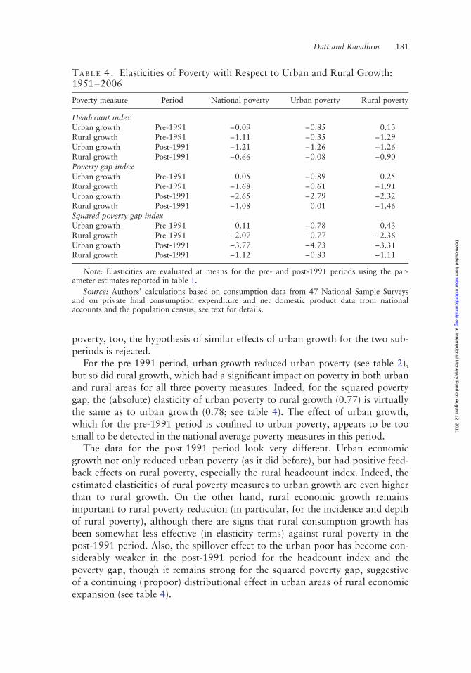
poverty, too, the hypothesis of similar effects of urban growth for the two sub-periods is rejected.

For the pre-1991 period, urban growth reduced urban poverty (see table 2),but so did rural growth, which had a significant impact on poverty in both urbanand rural areas for all three poverty measures. Indeed, for the squared povertygap, the (absolute) elasticity of urban poverty to rural growth (0.77) is virtuallythe same as to urban growth (0.78; see table 4). The effect of urban growth,which for the pre-1991 period is confined to urban poverty, appears to be toosmall to be detected in the national average poverty measures in this period.

The data for the post-1991 period look very different. Urban economicgrowth not only reduced urban poverty (as it did before), but had positive feed-back effects on rural poverty, especially the rural headcount index. Indeed, theestimated elasticities of rural poverty measures to urban growth are even higherthan to rural growth. On the other hand, rural economic growth remainsimportant to rural poverty reduction (in particular, for the incidence and depthof rural poverty), although there are signs that rural consumption growth hasbeen somewhat less effective (in elasticity terms) against rural poverty in thepost-1991 period. Also, the spillover effect to the urban poor has become con-siderably weaker in the post-1991 period for the headcount index and thepoverty gap, though it remains strong for the squared poverty gap, suggestiveof a continuing (propoor) distributional effect in urban areas of rural economicexpansion (see table 4).

TA B L E 4. Elasticities of Poverty with Respect to Urban and Rural Growth:1951–2006

Poverty measure Period National poverty Urban poverty Rural poverty

Headcount indexUrban growth Pre-1991 –0.09 –0.85 0.13Rural growth Pre-1991 –1.11 –0.35 –1.29Urban growth Post-1991 –1.21 –1.26 –1.26Rural growth Post-1991 –0.66 –0.08 –0.90Poverty gap indexUrban growth Pre-1991 0.05 –0.89 0.25Rural growth Pre-1991 –1.68 –0.61 –1.91Urban growth Post-1991 –2.65 –2.79 –2.32Rural growth Post-1991 –1.08 0.01 –1.46Squared poverty gap indexUrban growth Pre-1991 0.11 –0.78 0.43Rural growth Pre-1991 –2.07 –0.77 –2.36Urban growth Post-1991 –3.77 –4.73 –3.31Rural growth Post-1991 –1.12 –0.83 –1.11

Note: Elasticities are evaluated at means for the pre- and post-1991 periods using the par-ameter estimates reported in table 1.






Dow

nloaded from

Figure 3 shows the estimated impact of urban economic growth for theperiods before and after 1991. For each period, the figure plots the change inlog national headcount index that remains unexplained by rural growth againstthe change in log urban mean consumption. There was no significantpoverty-reducing effect of growth in mean urban consumption in the pre-1991period, but a significant impact emerges after 1991.

The qualitative results are generally robust to the choice of poverty measure.As in Ravallion and Datt (1996), the growth elasticities tend to be highest (inabsolute value) for the squared poverty gap and higher for the poverty gapthan for the headcount index. As in Ravallion and Datt, the higher growthelasticity of the poverty gap than the headcount index implies that growth alsoreduces the depth of poverty (as measured by the mean poverty gap relative tothe poverty line). Similarly, the even higher elasticity of the squared povertygap implies that growth reduces inequality among the poor (as measured bythe coefficient of variation). Thus, the impacts of growth within and betweensectors are not confined to households in a neighborhood of the poverty line.

There are two notable exceptions. The first is in the pre-1991 data for urbanareas, where a slightly lower elasticity is found for the squared poverty gap thanfor the poverty gap in the effects of urban growth on urban poverty (see table 4).This suggest an underlying adverse distributional effect among the poor in theurban economic growth process of the prereform period. The second exceptionis in the impacts of rural economic growth on rural poverty in the post-1991period, for the elasticity is lower for the squared poverty gap than for thepoverty gap in the post-1991 period (see table 4). It appears that an adverse dis-tributional effect among the rural poor has emerged in the rural growth processof the prereform period.

Compared with the earlier findings in Ravallion and Datt (1996), the moststriking new result is the evidence that the urban economic growth process since1991 has been appreciably more effective in reducing rural (and national)poverty. Since the regressions for rural poverty include rural mean consumption,the urban growth effect can be interpreted as a distributional effect. Supportiveevidence is provided by the following regression of changes in the rural log Giniindex (Gr) of inequality on the (share-weighted) urban and rural growth rates:38

D ln Grt ¼ 1:54

ð1:75Þð1� d91

t Þsmut�1D lnmut� 3:64

ð�1:68Þd91

t smut�1D lnmut

� 0:20ð�1:13Þ

ð1� d91t Þs

mrt�1D lnmrtþ 1:48

ð2:50Þd91

t smrt�1D lnmrt

� 0:08ð�1:67Þ

DMRPt þ 1t R2 ¼ 0:32; n ¼ 41

ð7Þ

38. Population shift effects were included (as in equation 5.2), but they were insignificant and are

not reported. The share-weighted urban and rural growth terms are instrumented, as in table 3.





Dow

nloaded from

FIGURE 3. Poverty Impacts of Urban Economic Growth in India

Note: The shaded area shows the 95 percent confidence interval.Source: Authors’ calculations based on consumption data from 47 National Sample Surveys

and on private final consumption expenditure and net domestic product data from nationalaccounts and the population census; see text for details.





Dow

nloaded from

where dt91 ¼ 1 for the post-reform period. From equation (7) it can be seen that,

unlike in the pre-1991 period, higher growth rates of mean urban consumptionsince 1991 have reduced inequality in rural areas (significant at the 10 percentlevel). Rural consumption growth, on the other hand, has had the oppositeeffect.

Implications of Measurement Errors

Concerns about underestimation of consumption in the NSS have implicationsfor assessing how the urban-rural composition of growth has affected poverty.The proportionate bias in the NSS estimates of mean consumption may well begreater in India’s urban areas, where (as noted) it is widely thought that theNSS does not fully capture the consumption of the rich (notably for consumerdurables and celebrations).

Even so, the direction of any net bias in these estimates of the growth elas-ticity of poverty reduction is unclear a priori. There are three sources of poten-tial bias. First, greater measurement error in the log of mean consumption inurban areas than in rural areas would imply greater attenuation bias in the esti-mate of the impact of urban economic growth on poverty, leading to underesti-mation of the true elasticity, meaning that the true elasticity is more negative.Second, to the extent that the NSS is not fully capturing the growth in con-sumption by the relatively rich, the measured mean consumption growth ratefrom the surveys may be lower than the true rate.39 Call this the “growth-ratebias.” This will partly or even fully offset the attenuation bias; indeed, if theeffect is strong enough, the measurement error in the mean may lead to anoverestimate of the true elasticity, meaning that the true elasticity is less nega-tive. Third, some of the bias in estimating mean consumption will be passedonto the poverty measures—also pushing toward overestimation of the elas-ticity. This can be called the “spillover bias.” The net effect of these threepotential sources of bias is unclear.

Nor is it clear how much all of this would matter to the comparison of elas-ticities between the pre-and post-1991 periods. Since the balance of theseeffects cannot be determined on theoretical grounds, the conclusion that urbaneconomic growth has become more poverty reducing may not be robust to cor-recting for measurement error in the NSS. The spillover bias is unlikely to bestrong, since it is consumption by the urban nonpoor that tends to be underes-timated by the NSS; correcting for this bias would not have much effect on thepoverty measures. However, by the same logic, the growth rate bias could belarge, and so there can be no presumption that the attenuation bias woulddominate.

39. In more technical terms, the measurement error in the NSS mean is not just a simple additive

error in the log mean, as in the standard formulation of the attenuation bias in a regression coefficient

due to additive measurement error in the regressor.





Dow

nloaded from

It could be argued that measurement error in the NSS has become a biggerproblem in more recent years. That conjecture is at least consistent with theincreasing divergence between the NSS mean and the NAS consumption aggre-gates, although this divergence could also stem from a rising share of the com-ponents of consumption included in the NAS aggregates that are not includedin the NSS (including measurement errors in the NAS). Evidence is found of alower elasticity of NSS consumption to NAS consumption in the postreformperiod, although the difference is small and not statistically significant.40

However, this would presumably strengthen both the attenuation bias and thegrowth rate bias, leaving the net effect indeterminate.

I V. C O N C L U S I O N S

While progress against poverty has been uneven, the long-run trend has been adecline in all three poverty measures based on a new time series of survey-based poverty measures for urban and rural India spanning 50 years, including15 years after economic reforms started in earnest in the early 1990s.Exponential (proportionate) trends are higher for the poverty gap and squaredpoverty gap indices than for the headcount index, reflecting gains to thoseliving well below the poverty line. Both urban and rural poverty measures haveshown a trend decline; rural poverty measures have historically been higherthan urban measures, though the two have been converging over time.

Progress against poverty has been maintained in the postreform period.Indeed, there was a higher proportionate rate of progress against poverty after1991, although the difference in trend rates of change between the two periodsis statistically significant only for the headcount index. The linear trend—theannual percentage point reduction in the poverty measures—remained aboutthe same in the postreform period. The responsiveness of poverty to growth inthe survey mean—the growth elasticity of poverty reduction—has also gener-ally remained the same between the two periods; only for the headcount indexis there a significant increase in the absolute growth elasticity in the postreformperiod. When growth as measured in the NAS is used, there are signs that thepostreform growth process has become less propoor in the sense of attaining alower proportionate rate of poverty reduction from a given rate of growth. Thisseems to be the result largely of the faster postreform growth not being fullyreflected in the surveys, and of the increase in inequality during the postreformperiod. The data do not make a robust case for saying that the growth elasticityof poverty reduction has risen (or fallen) since the reforms began.

40. The elasticities obtained by regressing consumption growth from the NSS on consumption

growth from the NAS (with controls for changes in whether the round used a mixed-recall period and

for changes in the log ratio of the rural price index to the NAS deflator) indicate that the elasticity is

lower in the post-1991 period, declining from 0.57 (4.47) in the pre-1991 period to 0.45 (t ¼ 3.29).

However, the null hypothesis that the elasticities for the two subperiods are the same cannot be

rejected.





Dow

nloaded from

Recognizing that the fortunes of the poor in urban and rural areas arelinked in various ways—through trade, migration, and transfers—this studyalso revisited earlier (prereform) findings on the relative importance of growthin urban and rural areas to poverty reduction in both areas and nationally(Ravallion and Datt 1996). Like that 1996 study, this one finds that the patternof growth matters for poverty reduction. But it also finds a striking change inthe relative importance of urban and rural economic growth in the postreformperiod. The 1996 study found that urban economic growth helped reduceurban poverty but brought little or no overall benefit to the rural poor; themain driving force for overall poverty reduction was rural economic growth.This study confirms that finding for the data up to 1991, but the picturechanges after 1991. As before, urban growth reduced urban poverty, and ruralgrowth reduced rural poverty. But there is much stronger evidence of a feed-back effect from urban economic growth to rural poverty reduction in thepost-1991 data than was found in the pre-1991 data. There are also signs thatthe post-1991 rural growth has been less poverty reducing in rural areas.

The relatively weak performance of India’s agricultural sector and the widen-ing disparities between urban and rural living standards remain important con-cerns, including for India’s poor. However, it is encouraging that rising overallliving standards in India’s urban areas in the postreform period appear to havehad significant distributional effects favoring the country’s rural poor. While theattribution of this effect to the reforms is hardly conclusive—since there can beno comparison group for India after 1991 without the reforms—these findingsare consistent with the view that with India’s efforts to create a more open andproductive market economy has come a reversal in the historical pattern ofweak feedback effects of urban economic growth on rural living standards.

This may be a surprising conclusion considering that sectors that rely onskilled labor have been the most dynamic. However, the more relevant obser-vation is that the nonfarm sectors that use unskilled labor more intensively—notably trade, construction, and the “unorganized” manufacturing sectors—haveseen higher employment growth in the postreform period. This is plausibly themain reason behind the stronger spillover effect of urban economic growth on therural distribution of levels of living since 1991. This encouraging finding comeswith a warning, however. While the rural poor have benefited more from urbaneconomic growth in the postreform economy, it can also be expected that theywill be more vulnerable in the future to urban-based economic shocks.

RE F E R E N C E S

Ahluwalia, Montek S. 1978. “Rural Poverty and Agricultural Performance in India.” Journal of

Development Studies 14 (3): 298–323.

——— 1985. “Rural Poverty, Agricultural Production, and Prices: A Reexamination.” In Agricultural

Change and Rural Poverty: Variations on a Theme by Dharam Narain, ed. J.W. Mellor, and G.M.

Desai. Baltimore, MD: Johns Hopkins University Press.





Dow

nloaded from

——— 2002. “Economic Reforms in India: A Decade of Gradualism.” Journal of Economic

Perspectives 16 (2): 67–88.

Banerjee, Abhijit, and Thomas Piketty. 2005. “Top Indian Incomes: 1956–2000.” World Bank

Economic Review 19 (1):1–20.

Bell, Clive, and R. Rich. 1994. “Rural Poverty and Agricultural Performance in Post- Independence

India.” Oxford Bulletin of Economics and Statistics 56 (2): 111–33.

Bhagwati, Jagdish. 1993. India in Transition. Oxford: Clarendon Paperbacks.

Bhattacharya, B., and S. Sakthivel. 2004. “Regional Growth and Disparity in India: Comparison of Pre-

and Post-Reform Decades.” Economic and Political Weekly 39 (10): 1071–77.

Bhattacharya, N., D. Coondoo, and R. Mukherjee. 1991. Poverty, Inequality and Prices in Rural India.

New Delhi: Sage Publications.

Boyce, James K. 1986. “Kinked Exponential Models for Growth Rate Estimation.” Oxford Bulletin of

Economics and Statistics 48 (4): 385–91.

Bruno, Michael, Martin Ravallion, and Lyn Squire. 1998. “Equity and Growth in Developing

Countries: Old and New Perspectives on the Policy Issues.” In Income Distribution and

High-Quality Growth, ed. Vito Tanzi, and Ke-young Chu. Cambridge, MA: MIT Press.

Chakravarty, Sukhamoy. 1987. Development Planning: The Indian Experience. Delhi: Oxford

University Press.

Chaudhuri, Shubham, and Martin Ravallion. 2006. “Partially Awakened Giants: Uneven Growth in

China and India.” In Dancing with Giants: China, India, and the Global Economy, ed. L. Alan

WintersShahid Yusuf, Washington, DC: World Bank.

Datt, Gaurav. 1997. “Poverty in India 1951–1994: Trends and Decompositions.” International Food

Policy Research Institute, Washington, DC.

Datt, Gaurav, and Martin Ravallion. 1992. “Growth and Redistribution Components of Changes in

Poverty: A Decomposition with Application to Brazil and India in the 1980s.” Journal of

Development Economics 38 (2): 275–95.

———. 1997. “Macroeconomic Crises and Poverty Monitoring: A Case Study for India.” Review of

Development Economics 1 (2): 135–52.

———. 1998. “Farm Productivity and Rural Poverty in India.” Journal of Development Studies 34 (4):

62–85.

———. 2002. “Has India’s Post-Reform Economic Growth Left the Poor Behind?” Journal of

Economic Perspectives 16 (3): 89–108.

Deaton, Angus. 2003. “Prices and Poverty in India, 1987–2000.” Economic and Political Weekly.

January 25.

———. 2005. “Measuring Poverty in a Growing World (or Measuring Growth in a Poor World).”

Review of Economics and Statistics 87 (1): 1–19.

———. 2008. “Price Trends in India and their Implications for Measuring Poverty.” Economic and

Political Weekly. February 9.

Deaton, Angus, and Jean Dreze. 2002. “Poverty and Inequality in India: A Re-Examination.” Economic

and Political Weekly. September 7.

Deaton, Angus, and A. Tarozzi. 2005. “Prices and Poverty in India.” In The Great Indian Poverty

Debate, ed. Angus Deaton, and Valerie Kozel. New Delhi: MacMillan.

Dreze, Jean, and Amartya Sen. 1995. India: Economic Development and Social Opportunity. Delhi:

Oxford University Press.

Eswaran, Mukesh, and Ashok Kotwal. 1994. Why Poverty Persists in India. Delhi: Oxford University

Press.

Foster, Andrew D., and Mark R. Rosenzweig. 2004a. “Agricultural Development, Industrialization and

Rural Inequality.” Brown University and Harvard University, Providence, RI and Cambridge, MA.

———. 2004b. “Agricultural Productivity Growth, Rural Economic Diversity, and Economic Reforms:

India, 1970–2000.” Economic Development and Cultural Change 52 (3): 509–42,





Dow

nloaded from

http://elibrary.worldbank.org/reference/matches?id=http://referencestore.ingenta.com/content/reference/0013-0079-2124C06A45CD17F8B054AAAAC38601FA-52-3-509--

Foster, James, J. Greer, and Erik Thorbecke. 1984. “A Class of Decomposable Poverty Measures.”

Econometrica 52 (3): 761–65.

Gaiha, Raghav. 1995. “Does Agricultural Growth Matter to Poverty Alleviation?” Development and

Change 26 (2): 285–304.

Heltberg, Rasmus. 2004. “The Growth Elasticity of Poverty.” In Growth, Inequality and Poverty, ed.

Anthony Shorrocks, and Rolph Van Der Hoeven. Oxford: Oxford University Press.

India, Planning Commission. 1979. Report of the Task Force on Projections of Minimum Needs and

Effective Consumption. New Delhi.

———. 1993. Report of the Expert Group on Estimation of Proportion and Number of Poor. New

Delhi.

———. 2009. Report of the Expert Group to Review the Methodology for Estimation of Poverty. New

Delhi.

Jacoby, Hanan, Mariano Rabassa, and Emmanuel Skoufias. 2010. “Distributional Implications of

Climate Change in India.” Development Research Group, World Bank, Washington, DC.

Jha, Raghbendra. 2000. “Growth, Inequality and Poverty in India. Spatial and Temporal

Characteristics.” Economic and Political Weekly. March 11.

Joshi, Vijay, and Ian Little. 1996. India’s Economic Reforms 1991–2001. Oxford: Clarendon Press.

Kakwani, Nanak. 1993. “Poverty and Economic Growth with Application to Cote D’Ivoire.” Review of

Income and Wealth 39 (2): 121–39.

Korinek, Anton, Johan Mistiaen, and Martin Ravallion. 2006. “Survey Nonresponse and the

Distribution of Income.” Journal of Economic Inequality 4 (2): 33–55.

Kotwal, Askok, Bharat Ramaswami, and Wilma Wadhwa. 2009. “Economic Liberalization and India

Economic Growth: What’s the Evidence?” University of British Columbia, Vancouver, BC.

Kuznets, Simon. 1955. “Economic Growth and Income Inequality.” American Economic Review 45

(1):1–28.

Lanjouw, Peter, and Rinku Murgai. 2009. “Poverty Decline, Agricultural Wages and Nonfarm

Employment in Rural India, 1983–2004.” Agricultural Economics 40 (2): 243–64.

Lipton, Michael, and Martin Ravallion. 1995. “Poverty and Policy.” In Handbook of Development

Economics Vol 3, ed. Jere Behrman, and T.N. Srinivasan. Amsterdam: North-Holland.

Panagariya, Arvind. 2008. India: The Emerging Giant. Oxford: Oxford University Press.

Purfield, Catriona. 2006. “Mind the Gap: Is Economic Growth in India Leaving Some States Behind?”

IMF Working Paper 06/103. International Monetary Fund, Washington, DC.

Ravallion, Martin. 2000. “Should Poverty Measures be Anchored to the National Accounts?”

Economic and Political Weekly. August 26.

———. 2003. “Measuring Aggregate Economic Welfare in Developing Countries: How Well do

National Accounts and Surveys Agree?” Review of Economics and Statistics 85: 645–52.

———. 2007. “Inequality is Bad for the Poor.” In Inequality and Poverty Re-Examined, ed. John

Micklewright and Steven Jenkins. Oxford: Oxford University Press.

Ravallion, Martin, Shaohua Chen, and Prem Sangraula. 2007. “New Evidence on the Urbanization of

Global Poverty.” Population and Development Review 33 (4): 667–702.

Ravallion, Martin, and Gaurav Datt. 1996. “How Important to India’s Poor is the Sectoral

Composition of Economic Growth?” World Bank Economic Review 10 (1): 1–26.

———. 2002. “Why Has Economic Growth Been More Pro-Poor in Some States of India than Others?”

Journal of Development Economics 68 (2): 381–400.

Saith, Ashwani. 1981. “Production, Prices and Poverty in Rural India. Journal of Development Studies

17: 196–213.

Sen, Abhijit. 2005. “Estimates of Consumer Expenditure and its Distribution. Statistical Priorities after

the NSS 55th Round.” In The Great Indian Poverty Debate, ed. Angus Deaton, and Valerie Kozel.

Delhi: Macmillan Press.





Dow

nloaded from

http://elibrary.worldbank.org/reference/matches?id=http://referencestore.ingenta.com/content/reference/0012-9682-D2112FEB856ECBB6D6ECC46C5DC6228D-52-3-761--

http://elibrary.worldbank.org/reference/matches?id=http://referencestore.ingenta.com/content/reference/0169-5150-9DC8C4E283A5D6F1BBFFB765B532A906-40-2-243--

http://elibrary.worldbank.org/reference/matches?id=http://referencestore.ingenta.com/content/reference/0304-3878-D03CCBB2192D8F24A3BC61041711A4A1-68-2-381--

Sen, Abhijit, and Hiamnshu. 2004a. “Poverty and Inequality in India 1.” Economic and Political

Weekly. September 18.

———. 2004b. “Poverty and Inequality in India 2: Widening Disparities During the 1990s.” Economic

and Political Weekly, September 25.

Sen, Amartya. 1976. “Poverty: An Ordinal Approach to Measurement.” Econometrica 46 (2): 437–46.

Sen, Kunal. 2009. “International Trade and Manufacturing Employment: Is India Following the

Footsteps of Asia or Africa?” Review of Development Economics 13 (4): 765–77.

Sundaram, K., and Suresh D. Tendulkar. 2001. “NAS-NSS Estimates of Private Consumption for

Poverty Estimation: A Disaggregated Comparison for 1993–94.” Economic and Political Weekly

January 13.

Vakil, C.N., and P.R. Brahmanand. 1956. Planning for an Expanding Economy. Bombay: Vora and

Company.

van de Walle, Dominique. 1985. “Population Growth and Poverty: Another Look at the Indian Time

Series Data.” Journal of Development Studies 21 (3): 429–39.

World Bank. 2005. World Development Report 2006: Equity and Development, Washington, DC:

World Bank.

———. Forthcoming. Perspectives on Poverty in India: Stylized Facts from Survey Data. Washington,

DC: World Bank.





Dow

nloaded from

Are The Poverty Effects of Trade Policies Invisible?

Monika Verma, Thomas W. Hertel, and Ernesto Valenzuela

Beginning with the WTO’s Doha Development Agenda and establishment of theMillennium Development Goal of reducing poverty by 50 percent by 2015, povertyimpacts of trade reforms have become central to the global development agenda. Thishas been particularly true of agricultural trade reforms due to the importance of grainsin the diets of the poor, presence of relatively higher protection in agriculture, as wellas heavy concentration of global poverty in rural areas where agriculture is the mainsource of income. Yet some in this debate have argued that, given the extreme vola-tility in agricultural commodity markets, the additional price and therefore povertyimpacts due to trade liberalization might well be indiscernible. This paper formallytests the “invisibility hypothesis” using the method of stochastic simulation in a trade-poverty modeling framework. The hypothesis test is based on the comparison of twosamples of price and poverty distributions. The first originates solely from the inherentvariability in global staple grains markets, while the second combines the effects ofinherent market variability with those of trade reform in these same markets. Results,at the national and stratum level indicate that the short-run poverty impacts of fulltrade liberalization in staple grains trade worldwide, are distinguishable in only four ofthe fifteen countries, suggesting that impacts of more modest agricultural tradereforms are indeed likely to be invisible in short run. Countries that show statisticallysignificant short run impacts are the ones characterized by high staple grains tariffsand/or a moderate degree of grain markets variability. Within each country, results areheterogeneous. In two thirds of the sample countries, agriculturally self-employedpoor experience statistically significant poverty impacts from trade liberalization.However, this figure is under a third for all the other strata. Agricultural trade reform,computable general equilibrium, poverty headcount, volatility, stochastic simulation,hypothesis testing. JEL codes: C12, C68, F17, I32, Q17, R20

Monika Verma (corresponding author: [email protected]) is Post-Doctoral Research Associate,

Center for Global Trade Analysis, Department of Agricultural Economics, Purdue University. Thomas

Hertel ([email protected]) is Distinguished Professor, Department of Agricultural Economics, and

Executive Director, Center for Global Trade Analysis, Purdue University. Ernesto Valenzuela (ernesto.

[email protected]) is Senior Lecturer and Executive Director, Centre for International

Economics, University of Adelaide.

The authors wish to thank Antoine Bouet, Paul Preckel, William Masters, Alain de Janvry and three

anonymous referees for helpful suggestions which led to significant improvements of this manuscript. A

supplemental appendix to this article is available at https://www.gtap.agecon.purdue.edu/resources/

res_display.asp?RecordID=3386

THE WORLD BANK ECONOMIC REVIEW, VOL. 25, NO. 2, pp. 190–211 doi:10.1093/wber/lhr014Advance Access Publication May 17, 2011# The Author 2011. Published by Oxford University Press on behalf of the International Bankfor Reconstruction and Development / THE WORLD BANK. All rights reserved. For permissions,please e-mail: [email protected]

190

World Trade Organization’s (WTO) Doha Development Agenda, and theMillennium Development Goal to reduce poverty by 50 percent by the year2015, served to bring the poverty impacts of trade reforms into central focusfor global policy makers. This has been particularly true of agricultural tradereforms due to the importance of grains in the diets of the poor, relativelyhigher protection in agriculture, as well as the heavy concentration of globalpoverty in rural areas where agriculture is the main source of income. Threequarters of the world’s poor reside in rural areas (World DevelopmentReport 2008), mostly depending for their livelihoods on agriculture; it istherefore hardly surprising that changes in primary commodity prices havebeen identified as one of the most important linkages between internationaltrade and poverty (Winters 2000). Agricultural commodity prices are ofcourse inherently volatile, due to the combination of inelastic demand andsupply, high perishability, high transport costs, and exposure to randomweather shocks. The recent 2007/2008 food price spike,in fact, has been esti-mated to have thrown more than one hundred million people temporarilyinto poverty (Ivanic and Martin 2008).

Given this background volatility in agricultural prices and poverty, somehave argued that the additional poverty impacts due to trade liberalizationmight well be indiscernible. Indeed, in a critique of an early draft of Clines(2004) book on trade policy and poverty, Rodrik (2003) made the point thatthe impacts of reforming agricultural protection in developed economies onworld prices are likely to be dwarfed by the inherent volatility of agriculturalmarkets. Similar sentiments surfaced in the context of the debate over thepoverty impacts of trade liberalization under the Doha Development Agenda(Hertel and Winters 2006). This paper terms this assertion, the ‘invisibilityhypothesis’. The goal of this paper is to formally test the invisibility hypothesisusing a model of global trade, linked to poverty modules for fifteen developingcountries.

It is important to point out up front that statistically failing to reject theinvisibility hypothesis by no means implies that agricultural trade reform iseconomically irrelevant. Even in cases where the long run impacts of agricul-tural trade reform are large, and of lasting importance, the short run impactsof such reforms on poverty might be statistically indiscernible due to theextreme volatility in international agricultural markets. As witnessed in recentyears, commodity price swings of more than one hundred percent within agiven year are not uncommon. These swings can themselves have a devastatingeffect on the poor – and they can also benefit those households which are netsellers of agricultural products. Given the significance of such commoditymarket volatility for the poor, it is important to couch agricultural tradereforms in this context. Also, the fact is that such reforms do not take place ina vacuum, and the presence of extreme market volatility will shape the way theworld perceives them. It is important that those advocating agricultural trade

Verma, Hertel, and Valenzuela 191

reforms not overstate the near term impacts, which may indeed be dominatedby other factors. On the other hand, it is also important to consider that, whilethe poverty changes induced by trade reforms may in some cases be smallerthan those swings caused by inherent commodity market volatility, the gainsfrom trade policy reforms represent permanent changes and are therefore likelyto be of greater economic significance than the transitory changes induced byannual market volatility.

Previous literature on poverty impacts of trade reforms in the presense ofinherent price variability is limited (Valenzuela 2009). Bourguignon et al.(2004) developed a stylized framework to assess the impact of export pricevariability on household income volatility. The related topic of the impact ofhigher food prices on poverty has also drawn attention (de Janvry and Sadoulet2010; Ivanic and Martin 2008) as have the impacts of trade reforms on incomedistribution (Robbins 1996; Lunati and OConnor 1999). However, none ofthese authors have offered a formal test of the invisibility hypothesis. The con-tribution of this paper is to provide such a test. The invisibility hypothesis isformulated as follows: Due to the high degree of volatility inherent in agricul-tural commodity markets, the incremental impact of agricultural trade liberali-zation on agricultural prices and the ensuing poverty impacts will bestatistically invisible.

The focus is on a subset of commodities – staple grains – which are oftensubject to high levels of protection, and which also represent a large share ofthe budget for the poorest households. Volatility in staple grains production ismodeled by sampling from a distribution of productivity shocks derived from atime series analysis of Food and Agriculture Organization (FAO) productiondata. This supply-side volatility is implemented in a Computable GeneralEquilibrium (CGE) framework – the agriculture-specific GTAP-AGR model(Keeney and Hertel 2005). The general equilibrium approach permits us tocapture the implications of changes in national commodity and factor prices,resulting from changesin global trade policies as well as uncertainty in worldgrain yields, while retaining economy-wide consistency. Our analysis concen-trates on the implications of these earnings and price changes, for the utility ofhouseholds in the neighborhood of the poverty line, asking whether they mightfall below this poverty line or be lifted out of poverty as a result of these com-modity market shocks. By aggregating across the diverse socio-economicgroups within the economy, a conclusion about the change in national povertyheadcount can be inferred for each draw from the agricultural productivity dis-tribution. The resulting distribution of poverty headcounts is contrasted withthe same distribution when trade reforms are implemented in combinationwith the inherent commodity productivity volatility. The first set of results,stemming from the inherent variability in global staple-grains markets, isreferred to as the stochastic baseline scenario, while the combined effects of theinherent market variability and trade reforms is referred to as the stochasticpolicy reform scenario. While the model is general equilibrium in nature, price


volatility only in the staple grains markets is considered and therefore, to beconsistent, the trade reforms are also only implemented in the staple grainssector. A further qualification stems from the fact that this is a static approach.Clearly a dynamic stochastic model would be preferred. This would permit usto distinguish permanent from transient shocks, with important implicationsfor agents’ responses to these different types of shocks. However, this wouldintroduce additional complexities that exceed the scope of this paper.

In order to get an adequately broad representation of the diverse economiesand circumstances in which the world’s poor live, this analysis is undertakenfor fifteen developing countries in South Asia, Latin America and Sub-SaharanAfrica. The remainder of this study is organized as follows. The methodologyis described next (Section I). Section II presents the results for the moments ofdistributions for variables driving poverty headcounts changes before formallytesting the invisibility hypothesis. It also provides a discussion of sensitivity ofour results to the assumption of exogenous trade policy changes. Caveats, con-clusions and policy implications are discussed last (in Section III).

I . M E T H O D O L O G Y

One approach to testing the invisibility hypothesis would be to develop asingle country trade/poverty model in great detail and test this hypothesis inthe context of that particular country. This is attractive, as it would allowdevelopment of the poverty component in considerable detail (see Hertel andWinters 2006, for ten country case studies undertaken to assess the nationalimpacts of WTO reforms). However, there are several problems with thisapproach. Firstly, using a national model makes it difficult to generate stochas-tic global price shocks in a consistent manner. Secondly, WTO agriculturalreforms typically entail significant liberalization in developed markets, sowithout a global framework it is problematic to accurately assess the povertyimpacts of such reforms on developing countries. Finally, readers would verylikely argue that the results were specific to the country under investigation, ifsuch tests of the invisibility hypothesis were undertaken only for an individualcountry. Therefore, a multi-country approach to testing the invisibility hypoth-esis is adopted. The cost of doing so is that the poverty analysis is necessarilyrather simple and symmetric across countries.

Poverty Headcount Analysis

The analysis here relies on the trade/poverty approach outlined in Hertel et al.(2009). Those authors focus on poverty headcount changes in diverse house-hold population strata across a range of developing countries. A first orderapproximation to such poverty headcount changes may be written as follows


(the hats denote percentage changes in the associated variables):

Hrs ¼ �1rs � yprs ¼ �1rs �

Xj

aprsjðwrj � Cp

r Þ: ð1Þ

Here, the index r denotes region (focus country), s the population stratum1

and the superscript p signifies that the variable in question is associated withearnings and consumption patterns at the poverty level of utility. Any shock tothe economy that alters the after-tax returns to factor j (wrj) and/or the pricesof consumption goods, will affect the poverty level of income (yrs

p ), the cost ofliving for poor households (Cr

p) and therefore strata poverty headcounts (Hrs).The term

Pj a

prsjðwrj � Cp

r Þ in equation (1) is the percentage change in realfactor income in stratum s of region r, taking into account the cost of livingchanges for households at the poverty line in stratum s of region r. The change

in cost of living at the poverty line in region r, denoted Cpr , is the change in

household expenditure required to keep utility constant at its poverty level,once a new set of prices is obtained. This change is derived by solving thehousehold expenditure minimization problem at the new prices, while keepingutility fixed at the poverty level. Thus households are permitted to alter theiroptimal consumption bundle in response to the new commodity prices.

Apart from the “driver” variables (after-tax factor earnings and commodityprices), two more elements play an important role in determining poverty head-count impacts. Coefficient arsj

p is the share of factor earning j in total incomefor households at the poverty line, in stratum s of region r. For a given increasein factor earnings (e.g., unskilled agricultural labor), a stratum that obtains 90percent of its income from this concerned factor, will experience a greaterincome rise than one with only 10 percent of its income attributable to thatfactor. Since these are shares, the summation over factor earnings types for anygiven stratum equals one (

Pj a

prsj ¼ 1). The values for arsj

p in our sample of 15countries are obtained from household surveys and range from 0 to 0.99 (asshown in Appendix Table A1, available at https://www.gtap.agecon.purdue.edu/resources/res_display.asp?RecordID=3386). The second coefficient ofinterest in equation (1) is 1rs, the poverty elasticity with respect to income instratum s of region r. The higher the poverty elasticity, the greater the head-count reduction from a given increase in income for households at the povertyline in that particular stratum. Estimates of 1rs range from 0.0006 to 8.9(Appendix Table A2), and vary widely by stratum and country.2

The change in total poverty headcount in a region is obtained by summingover stratum headcounts; therefore, the percentage change in national head-count can be written as share weighted sum of percentage headcounts changes

1. There are seven strata: Agriculturally self-employed, non-agriculturally self-employed, rural wage

labor, urban wage labor, rural diversified, urban diversified and transfer stratum.

2. More details on the elasticities can be found in Verma et al. (2011).


at the stratum level:

Hr ¼X

s

brs�Hrs; ð2Þ

where the shares (brs) are the share of stratum s in total poverty in the region r.brs plays an important role in determining how the stratum headcount changesget translated into the aggregate regional headcount.3 The initial equilibriumvalues for all of these coefficients are estimated from household survey data forthe 15 focus countries (Hertel et al. 2004) and are reported in AppendixTable A2.

Substituting equation (1) in (2) gives the regional headcount in terms of itsdriving factors

Hr ¼ �X

s

brs � 1rs �X

j

aprsjðwrj � Cp

r Þ; ð3Þ

(3) can be further decomposed into changes due to pre-tax factor earnings(wm

rj ¼ wrj þ Tr), income tax changes (Tr) designed to ensure revenue neutralityof policy and the cost of living changes due to changed consumption prices,evaluated relative to the change in net national income:

Hr ¼ �X

s

brs � 1rs �X

j

aprsj wm

rj � yr

� �þ 1r � Tr þ 1rðCp

r � yrÞ: ð4Þ

The first term in equation (4) can be termed the earnings effect and involvesthe changes in factor earnings of the poor relative to national income. Thesecond term is the tax effect and the last term identifies the effect of changes incost of living relative to net national income. The term 1r is the regionalpoverty elasticity and is defined as the poverty share-weighted sum of stratapoverty elasticities (

Ps brs � 1rs). Any increase in taxes or relative cost of living

raises poverty headcount in a region while increased relative factor incomeswork towards poverty reduction. Overall, the poverty headcount in stratum sof country r falls when real income increases; the amount by which it fallsdepends on the density of the population in the neighborhood of the povertyline.

Equation (4) offers a useful framework for analyzing the poverty impacts oftrade and commodity market volatility. There are, however, some importantlimitations to its use which deserve a mention. Foremost among these is the

3. Consider for expository purposes that the poverty headcount for the rural diverse stratum for

both Brazil and Uganda fell by 50 percent and other strata were unaffected (Hrs ¼ 0 8s = ruraldiverseÞ,then regional poverty headcount in Brazil would fall by a mere 1.5 (0.03 x 50) percent while in Uganda

by a 37.5 (0.75 x 50) percent. The results are so diverse due to the big difference (0.03 versus 0.75) in

the share of poverty population concentrated in the rural diverse stratum in the two countries, as can be

seen from Appendix Table A2.


static composition of the strata as the earnings specialization of householdsisn’t allowed to change; large shocks may induce a household to switchemployment (e.g. moving from agriculture to non-agriculture), although this isless likely in the short run. In addition, the focus is only on changes in thepoverty headcount; ignoring higher order measures, such as the poverty gap.The virtue of this simple approach is that it can be readily implemented acrossa wide range of household strata and countries, thereby permitting us to gener-alize our findings.

Global General Equilibrium Model

To calculate the impact of trade policy reforms on poverty headcount as perequation (4), one must first determine the impact of trade policy reforms onthe poverty “drivers”, wrj and Cr

p. The inability of partial equilibrium frame-works to predict the changes in economy-wide factor returns, which play avery prominent role in the analysis, forces us to use a CGE model in our analy-sis. One of the main criticisms of CGE models is the absence of validation(Kehoe et al. 1995). Accordingly, special attention is devoted to validating themodel with respect to staple grains markets.

This study employs the GTAP-AGR model of Keeney and Hertel (2005)which is explicitly designed to focus on issues of agricultural trade liberaliza-tion. (See Appendix I for details on the model structure and data sources used).A short-run factor market specification is used such that land is commodity-specific, capital is sector-specific and labor is imperfectly mobile between agri-culture and non-agriculture sectors. The degree of inter-sector mobility is deter-mined by the choice of relevant parameters in the model. These are set, basedon evidence on labor mobility from the OECD (2001). In addition, the modelis modified to accommodate the replacement of lost tax revenue from tradereforms, in the form of a non-distorting uniform ad valorem tax on income,making each scenario fiscally neutral.

Stochastic Simulation and Model Validation

The credibility of any simulation model hinges very much on whether themodel can produce reliable predictions for key endogenous variables, based onhistorical shocks. In practice, there are very few natural experiments involvingtrade policy reforms. WTO rounds are typically concluded once every decadeor two, and their implementation is gradual and fraught with controversy.National reforms are sometimes more clear-cut; however, their effects are oftenconfounded with other significant events (e.g., a financial crisis, or a recession,etc.). Therefore a different type of natural experiment which is somewhatunique to the staple grains markets, is used for validation – the focus is onhow well the model captures the economic impacts of random historic vola-tility in agricultural productivity, largely induced by weather-related shocks.Given the relative stability of demand for subsistence goods such as staplegrains, demand-side volatility is ignored here; characterizing only supply side


volatility in the staple grains markets and thereupon asking whether the modelis capable of reproducing observed price volatility in these same markets. If themodel can accurately characterize inter-annual price volatility in response tosupply side shocks then it is also a valid tool for looking at the short runimpacts of tariff shocks in these same markets.

The validation approach involves using production shocks derived from theresiduals of time series models of FAO grains production data. By samplingfrom the derived distribution, the stochastic simulation seeks to mimic the ran-domness inherent in these markets. Solving the CGE model repeatedly, eachtime with a different set of productivity draws, produces the resulting distri-bution of price changes for each region. The validation then involves compar-ing the model results for grain price variation, with FAO observed pricevariation in each region. With the aim of improving the CGE replication ofobserved FAO price variability, the model’s consumer demand elasticities wereadjusted for a few regions; details of the approach are given in the next sub-section. After ensuring the historic price variation is faithfully replicated, onecan concentrate on contrasting the poverty headcount distributions associatedwith the stochastic baseline and stochastic policy reform scenarios and testingfor statistical difference between these two sets of results.

Characterizing Volatility. Tyers and Anderson (1992) characterize uncertaintyin global food markets by sampling from a distribution of supply shocks.Valenzuela et al. (2007) use this approach to validate a model of global wheattrade. The same approach has been used here. Autoregressive Moving Average(ARMA) models are used to characterize systematic changes in staple grains pro-duction, using the ARMA residuals to define the distributions of productivityshocks. This specification is appealing in modeling grain crops productionbecause past values appear to carry a great deal of information about currentvalues and prediction errors arise largely from weather-related shocks to pro-duction. Staple grains production data from the FAO for the period 1991 to 2006(FAOSTAT)4 is used to calculate the productivity shocks for aggregate regions.5

The 15 focus countries inherit the shocks from their respective parent region.The model selection is guided by the significance of the AR and MA com-

ponents, the Akaike Information Criteria (AIC), and autocorrelation inresiduals for alternative model specifications. The normalized standard devi-ations of the production residuals from the estimated time series models areused to create a distribution reflecting random regional productivity variation.

4. While paddy rice and wheat are the same across GTAP and FAOSTAT terminology, the

Coarse-grains category under GTAP covers barley, maize, mop corn, rye, oats, millet, sorghum,

buckwheat, quinoa, fonio, triticale, canary seed, mixed grain and cereals nes. reported in FAO data.

5. Calculations using FAOSTAT data show that measures of observed volatility in output vary

considerably depending what aggregation of crops and regions is used. Generally speaking, the higher

the level of aggregation, the lower is the volatility that the CGE model is adjusted to replicate. The

aggregation scheme for regions is provided on Appendix Table A4.


The greatest production volatility is seen in Russia6, Sub-Saharan Africa andEastern Europe. With the assumption that productivity follows a symmetric tri-angular distribution, the end points of this distribution are determined by theformula: mean+

ffiffiffi6p� productivity standard deviation. This estimated distri-

bution of productivity shocks for each region provides the basis for implement-ing the stochastic baseline scenario.

The methodology involves sampling from this distribution of productivityshocks and solving the CGE model repeatedly. The results for each solve of themodel are stored and the means and standard deviations of the stored resultsfor all endogenous variables are calculated. The sampling is done by means ofGaussian Quadrature (GQ), a numerical integration technique developed as analternative to Monte-Carlo simulations, and implemented for GTAP models byPearson and Arndt (2000). The GQ technique is chosen instead of the moretraditional Monte Carlo approach, as it significantly reduces the number ofsimulations while still preserving the accuracy of the resulting means and stan-dard deviations for endogenous variables (DeVuyst and Preckel 1997).

The validity of evaluating the impacts of trade liberalization in the context ofa volatile grains market environment critically depends on the capability of theCGE system to replicate historical price variability. This capacity of the model isassessed by comparing the model simulated volatility for staple-grains prices, toFAO-observed volatility (Table 1). Since staple grains represent a composite ofmany commodities, a range of historic price volatilities from the FAO data baseis reported in the first column of this Table. For example, in Bangladesh, pricevolatility of rice, wheat and coarse-grains, as measured by the normalized stan-dard deviation of ARMA residuals, ranges from 5% to 12%. In the Philippines,this is a smaller range (10% to 13%). Initial results indicated that the modeloverstated price volatility for Philippines, Bangladesh, Colombia, Peru,Venezuela, Malawi and Mozambique; while it understated the same forThailand. Aiming to replicate the price volatility for these regions more closely,the consumer demand elasticities in these regions were re-calibrated.7

Specifically, demand elasticities were increased for regions where price volatilitywas over-predicted by the model, while they were reduced for Thailand.Elasticities were also increased for all the rest of Sub-Saharan African regions, asthe model predicted unusually high price volatility for these countries.

The price volatility results, after adjusting the elasticities, are reported forcomparison (Table 1). This calibration process enables the CGE model toreplicate the FAO data price variation in most cases (with the exceptions ofThailand, Colombia and Venezuela). For Colombia and Venezuela the modelover-states price volatility. This could be due to the Andean Price Band

6. This region includes Russia and all the constituent states of the former Soviet Union.

7. More details and justification for this approach is provided in Verma (2010).


System policy which was implemented in 1995 and involved variable tariffs inPeru8, Colombia, Venezuela and Ecuador aimed at restricting price fluctu-ations in these markets (Villoria et al. 2002). The model used here does notreflect these country specific policies and therefore misses these effects.9 ForThailand the model under-predicts price volatility – a problem similar to thatfaced by Valenzuela et al. (2007) who found that the same type of globalCGE model under-predicted price variations for most exporters (Thailand is amajor exporter of rice). The base case scenario here does not incorporate theendogenous response of border policies to changes in global market conditionsuch as the export bans and import policy changes which arose in thecontext of the 2007/2008 food crisis. These policies tend to exacerbate pricevolatility – particularly for exporters (see Valenzuela et al. for more details).Implications of such policy endogeneity are briefly explored in Section IIIbelow.

TA B L E 1. Historic versus Model Generated Price Volatility and AssociatedPercentage Changes in Poverty Headcount

HistoricVolatility Range

Model GeneratedVolatility Results

Mean PercentChange (stochastic baseline)**

Bangladesh 5-12 11 0.19Indonesia 9-19* 11 0.07Philippines 10-13* 13 20.10Thailand 11-14 7 0.02Vietnam � 7 0.18Brazil 11-20 12 0.09Chile 7-21 11 0.03Colombia 4-10 14 0.07Mexico 7-9 9 0.12Peru 6-15 15 0.08Venezuela 6-11 18 0.12Malawi 21-30 23 20.01Mozambique 16-20 19 0.12Uganda � 22 20.07Zambia � 19 0.12

Source: FAO Price-Stat Data 1991-2006, Model generated price variation results and AuthorsCalculations using Model Simulation Results

* FAO Price data on wheat is not available for Indonesia and Philippines; so the range reflectsthe price volatility of rice and coarse grains only.

� FAO Price data on none of the crops is available for Vietnam, Uganda and Zambia.

** These changes in Poverty Headcount in absence of any policy shock arise as a result ofinherent changes in agricultural commodity prices.

8. In the case of Peru, the model generated price variation reaches the upper limit of the observed

price variation range.

9. In principle it would be desirable to model these policies explicitly. However owing to the diverse

range and complexity of policies across countries, such an endeavor is better-suited to a country case

study approach.


With mean zero agricultural productivity shocks under the stochastic base-line, mean zero outcomes for most model variables are to be expected. The lastcolumn of Table 1 in fact shows that the mean changes for the poverty head-counts10 are less than 1 percent.

Modeling Staples Trade reforms. The year 2001 is adopted as the bench-mark, as it is the base year for Doha proposals on tariff cuts and also the baseyear for the GTAP version 6.1 data (Dimaranan 2006). The first column ofTable 2 shows tariffs in the staple grains sector for all of the 15 focuscountries. Mexico has the highest import tariffs for staple grains, followed byThailand and Peru. Overall, the focus countries have much lower tariffs onstaple grains than do the non-focus countries (rest of world). This study con-siders a scenario of trade liberalization which involves the complete removal oftariffs in all focus, as well as non-focus countries.11 Though our simulationsfocus on full liberalization in all countries, under realistic trade negotiationsdifferent countries may undertake different levels of agricultural tariffreductions. To be consistent with the stochastic baseline simulations (variabil-ity is restricted to staple grains production), trade reforms in other sectors ofthe economy are not considered. Thus, our stochastic policy reform scenario isthe combined effect of inherent market variability and the complete eliminationof effectively applied tariffs in staple-grains market.

I I . R E S U L T S

Elimination of the import tariffs for staple grains is expected to result in lowerconsumer prices in countries with high initial tariffs (see Table 2). Since theaverage import tariff in the focus regions is about 11 percent, countries withhigher than 11 percent tariffs are expected to experience greater consumerprice reductions, and therefore potential greater poverty reductions (abstractingfrom the earnings side of the poverty story). We focus on the impacts of tradereform in the context of the stochastic simulations.12

A good starting point – before focusing on poverty headcount distributions,at the aggregate regional as well as the disaggregated stratum levels – is the

10. Any big numbers in thousands of units can be explained by the presence of a big poverty base

(Appendix Table A5). Note that as the percent change in poverty headcounts is the average percentage

change in the variable across 22 simulations, the decomposition of results though along the lines of

deterministic setup is not as straightforward. Most of the analysis therefore focuses not on what is

driving the means but on a more relevant question that the stochastic framework can answer: whether

the distributions with and without reforms are different.

11. The focus is on tariffs-only policy reform as data on domestic support and export subsidies is

not available on a consistent global basis. Croser and Anderson (2010) using a partial equilibrium

framework and a recent World Bank comprehensive set of indicators of distortions to agricultural

incentives (Anderson and Valenzuela 2008) found that border measures in agricultural markets account

for more than 85 percent of global loss of welfare.

12. Readers interested in a detailed deterministic analysis of the impacts of tariff reform alone are

referred to Appendix II.


comparison of pre and post reform distributions of endogenous variables that“drive” the poverty headcount results. As indicated in equation (1), these arethe consumption prices and factor earnings.

Distributions of Driver Variables

The comparison of the mean and standard deviations of driving factors –staple grains consumption prices (affecting the cost of living) and real after taxfactor earnings (affecting income) – across the stochastic baseline and stochas-tic policy scenarios should provide insights into the results of formal test of thepoverty headcount distributions under the same scenarios. If the moments ofdistributions for these variables differ little across the two scenarios, thenresults for poverty headcounts will also very likely not be distinguishable.

TA B L E 2. Import Tariffs on Staples and Mean and Standard Deviations forStaples Prices (Percentage Change), Before and After Tariff LiberalizationUnder a Stochastic Scenario

Country(s)ts

Stochastic Baseline Scenario Stochastic Policy Scenario

(Tariffs) Mean Standard-Deviation Mean Standard-Deviation

Bangladesh 4.54 0.7 6.0 0.0 5.7Indonesia 1.47 0.9 7.7 24.0 6.3Philippines 6.19 1.1 6.1 212.1 4.7Thailand 20.42 1.1 4.4 25.0 5.7Vietnam 2.76 2.6 7.2 6.9 5.8Brazil 0.14 1.1 4.9 1.6 3.9Chile 6.98 1.0 9.4 0.7 9.2Colombia 12.77 0.5 3.8 22.8 3.6Mexico 23.94 0.9 8.6 210.9 7.2Peru 16.46 0.5 4.9 25.1 4.4Venezuela 12.10 1.2 9.7 21.1 9.4Malawi 0.08 4.0 20.6 3.1 19.9Mozambique 2.11 2.8 16.8 21.5 16.0Uganda 0.72 2.4 14.5 0.8 14.1Zambia 2.90 2.9 17.5 2.2 17.0Poverty Regions’ Average Tariff 11.39Average Tariff for other Regions 34.89World Average Tariff 30.65

Source: Calculations using GTAP Database version 6 for tariffs and using Model SimulationResults for others

The average applied import tariffs are calculated as

ts ¼X

i

Pr VIWirsP

r

Pi VIWirs

�X

r

VIWirsPr VIWirs

�tirs

� �" # !

where the Value of Imports (VIWirs) at World prices by commodity(i), source (r) and destination(-s);and the tariff rates (tirs) come from GTAP version 6 database.


Tables 2 and 3 present the results for these driver variables – staple con-sumption prices and factor incomes respectively – for all 15 countries. Forexample the mean staple grains consumption price in Mexico increases by 0.9percent under stochastic baseline while it falls by 10.9 percent under the sto-chastic policy scenario; so there is a difference of 11.9 percentage pointsbetween the two scenarios for Mexico. The same figure for Thailand is 25.0 –1.1 ¼ 23.9 percentage points (Table 2). For Mexico, most of the change isdriven by the reduction in prices as a result of removing high import tariffs inthe country. The increase in staples price in Thailand is driven by the increasedprice of rice owing to increase in rice export demand (Appendix II). Thereforms seem to benefit consumers in Latin America; as the mean staple pricesare lower (except for Brazil13) and no more volatile under the stochastic policyscenario as compared to the baseline scenario (Table 2). Also it is interesting tosee that, while mean outcomes (especially for staple grains) show some differ-ence, the standard deviations across the scenarios are very similar, this wesuspect, is partly due to the omission of endogenous trade policy responses toworld market price variability in this analysis. (This issue is explored in moredetail below.)

A similar comparison of after-tax real factor earnings is offered for the focuscountries (Table 3). The first panel in the table gives the percentage pointdifferences in means while the bottom panel gives the same for standard devi-ations. A positive number indicates that the post liberalization mean or stan-dard deviation for the factor endowment in a given country is higher thanunder the baseline (no liberalization) scenario. The changes in factor returns toland and agricultural capital are greater than those for other factors due totheir sector specificity and more limited factor mobility respectively. Also, aswith the results in Table 2, the changes in standard deviations are generallymodest.

Small changes in the standard deviation compared to the mean suggest thatthe Kolmogorov-Smirnov (henceforth KS) two sample test14 can be used as aformal test of difference in distributions of consumption prices and factor earn-ings. The KS test answers the question: are the observations under one scenariosystematically larger or smaller than under the other scenario? Test results forstaples consumption prices and factor earnings are provided in Appendix III.The main conclusion of the test is that, while some factors earnings are statisti-cally different post liberalization, this finding is by no means universal acrossfactors and countries. Given that strata are defined based on income specializ-ation, it is therefore likely that the results will show within-country, across-stratum differences in the visibility of poverty headcounts. The next section

13. The deterministic results in Appendix II show the reason for increased post liberalization prices

in Brazil on account of increased demand for coarse-grain exports from the country.

14. This test in comparison to other non-parametric tests performs better for cases where there is

not much difference in variance (Baumgartner et al. 1998).


TA

BL

E3

.D

iffe

rence

sin

Mea

nand

Sta

ndard

Dev

iati

ons

of

Rea

lA

fter

-Tax

Fac

tor

earn

ings

bet

wee

nSto

chast

icPolicy

and

Sto

chast

icB

ase

line

Sce

nari

os

(per

cent

changes

)

Bangla

des

hIn

dones

iaPhil

ippin

esT

hailand

Vie

tnam

Bra

zilC

hile

Colo

mbia

Mex

ico

Per

uV

enez

uel

aM

ala

wiM

oza

mbiq

ue

Uganda

Zam

bia

Mea

nL

and

21.0

22.5

23.9

15.4

4.5

1.4

21.7

20.7

22.1

22.5

20.7

21.7

21.4

20.6

21.3

Ag-U

nsk

ille

d0.0

20.4

0.2

1.4

0.5

0.0

20.1

0.2

0.4

0.0

0.0

20.2

0.3

0.0

0.0

Ag-S

kille

d0.0

20.1

0.9

0.9

0.4

0.0

20.1

0.2

0.5

0.0

0.0

20.1

0.4

0.1

0.1

NonA

g-U

nsk

ille

d0.2

0.7

1.9

22.1

20.2

0.0

0.1

0.3

0.8

0.4

0.1

0.0

0.5

0.2

0.2

NonA

g-S

kille

d0.2

0.8

2.1

22.2

20.1

0.0

0.1

0.3

0.8

0.4

0.1

0.0

0.5

0.2

0.2

Wage-

Unsk

ille

d0.2

0.5

1.2

21.5

20.1

0.0

0.1

0.3

0.8

0.3

0.1

20.1

0.4

0.1

0.1

Wage-

Skille

d0.2

0.8

2.1

22.2

20.1

0.0

0.1

0.3

0.8

0.4

0.1

0.0

0.5

0.2

0.2

Ag-C

apit

al

21.0

22.5

23.9

15.4

4.5

1.4

21.7

20.7

20.6

22.6

20.7

21.7

21.4

20.6

21.4

Nag-C

apit

al

0.2

0.8

2.1

22.4

20.1

20.1

0.1

0.4

0.9

0.6

0.1

0.0

0.5

0.2

0.2

Tra

nsf

ers

0.1

0.5

1.2

21.0

0.2

0.0

0.0

0.3

0.8

0.3

0.1

20.3

0.3

0.0

0.1

Sta

ndard

Dev

iati

on

Land

20.7

20.7

21.2

1.8

22.4

0.0

20.1

0.1

20.2

20.8

20.1

0.2

20.3

20.5

20.3

Ag-U

nsk

ille

d0.0

0.0

0.3

0.1

0.0

0.0

0.0

0.0

0.0

20.1

0.0

0.6

0.1

0.0

0.1

Ag-S

kille

d2

0.1

0.0

20.3

0.1

0.0

0.0

0.0

0.0

0.0

20.1

0.0

0.5

0.0

20.1

0.2

NonA

g-U

nsk

ille

d2

0.1

20.2

20.5

0.0

20.3

0.0

0.0

0.0

0.0

20.1

0.0

0.4

0.0

20.1

0.1

NonA

g-S

kille

d2

0.2

20.2

20.6

0.0

20.3

0.0

0.0

0.0

0.0

20.1

0.0

0.4

0.0

20.1

0.1

Wage-

Unsk

ille

d2

0.1

20.1

20.4

0.0

20.2

0.0

0.0

0.0

0.0

20.1

0.0

0.5

0.0

0.0

0.1

Wage-

Skille

d2

0.2

20.2

20.6

0.0

20.3

0.0

0.0

0.0

0.0

20.1

0.0

0.4

0.0

20.1

0.1

Ag-C

apit

al

20.7

20.7

21.2

1.8

22.4

0.0

20.1

0.1

0.0

20.8

20.1

0.2

20.3

20.5

20.3

Nag-C

apit

al

20.1

20.2

20.4

0.0

20.3

0.0

0.0

0.0

0.0

20.1

0.0

0.4

0.0

20.1

0.0

Tra

nsf

ers

20.1

20.1

20.2

20.1

20.1

0.0

0.0

0.0

0.0

20.1

0.0

0.1

0.0

0.0

0.0

Sourc

e:A

uth

ors

’ca

lcula

tions

Usi

ng

Model

Sim

ula

tion

Res

ult

s


offers a formal test of differences between poverty headcount distributions atboth the country and stratum levels.

Distribution of Poverty Headcounts

The KS test is implemented to formally compare the two distributions ofpoverty headcounts, resulting from stochastic baseline and stochastic policyreform scenarios. The null hypothesis is that the two distributions are not stat-istically different and are therefore hard to tell apart. Calculated KS test stat-istic values, along with the associated P-values are reported for all the focuscountries (Table 4). The table shows that poverty headcount changes followingtrade liberalization are statistically perceptible at a 10 percent level of signifi-cance, in just four countries: Indonesia, Chile, Peru and Mexico.

Figure 1 shows what the results look like graphically for two cases –Bangladesh and Mexico – one where the two distributions are not statisticallydistinct and the other where they are clearly differentiated. The lines in thefigure are the sample cumulative density functions (CDFs) for poverty head-count changes in the two countries under alternative scenarios. The sample

TA B L E 4. K-S Test Statistics, P-Values and Moments of Distributions Acrossthe Baseline and Policy Scenarios for Poverty Headcount Changes

Stochastic BaselineScenario

Trade Liberalizationin StochasticFramework

Calculated KSTest Statistic

(in thousands)

P-value MeanStandarddeviation Mean

Standarddeviation

Bangladesh 0.18 0.84 83 598 14 553Indonesia 0.41 0.04 10 41 25 31Philippines 0.27 0.39 211 277 98 262Thailand 0.18 0.63 0 7 1 8Vietnam 0.14 0.87 3 13 11 0Brazil 0.14 0.92 21 113 27 106Chile 0.36 0.06 0 3 2 3Colombia 0.32 0.20 3 16 26 16Mexico 0.64 0.00 11 104 2128 96Peru 0.36 0.06 3 24 29 20Venezuela 0.27 0.39 4 24 21 23Malawi 0.32 0.20 0 17 8 26Mozambique 0.23 0.57 7 46 26 48Uganda 0.27 0.39 212 14 25 9Zambia 0.14 0.92 7 59 2 62

Source: Authors’ calculations using Model Simulation Results

The negative numbers under the mean columns are to be interpreted as a reduction in povertyheadcount.


observations refer to the pooled samples generated by the repeated model simu-lations under the two stochastic scenarios (see Appendix III for technicaldetails). The maximum vertical distance between the two lines is the KS teststatistic. For Bangladesh, these sample CDFs lie very close together while theylie farther apart and do not overlap for Mexico. The samples in question arethose generated under the stochastic baseline and under stochastic trade liberal-ization. The figure brings out the nature of our results very clearly – the effectsare visibly distinct in one case while not in the other. This point is furtherunderscored via a set of diagnostic plots reported for all the sample countriesin Appendix IV.

FIGURE 1. Empirical Cumulative Distributions of Poverty Headcount Changesin Mexico and Bangladesh

Source: Model simulation results


The results of the KS test of the invisibility hypothesis for all seven strata ineach of the 15 focus countries are provided in Table 5. At the 10 percent levelof significance (p-value less than 0.1), for only 30 of the 105 country- stratumpairs the results turn out to be statistically distinct. Note that in Indonesia theheadcount changes are statistically visible only in the agricultural stratum;however because this stratum has a 42 percent share in the national povertyheadcount (Appendix Table A2), its statistical significance carries over to theoverall national-level invisibility hypothesis test results. Conversely, whilepoverty headcount changes are statistically significant for all but the rural andurban diverse strata in Philippines, the changes at the national level are not sig-nificant. This stems from the fact that the two diversified strata comprise over70 percent of Philippines’s poverty population (23 percent for urban diverseand 49 percent in rural diverse, as shown in Appendix Table A2). Two othercases that stand out in these results are Chile and Thailand. For Chile, whilethe national level impacts of trade reform are visible, only the agriculturalstratum is statistically significant and it makes up only 26 percent (AppendixTable A2) of the country’s poverty headcount. In Thailand, while all stratashow significantly perceptible poverty headcount results, the same does nothold for the national level results due to the fact that the agricultural head-count reductions are offset by the urban increases. The lower panel of Table 5sheds further light on this conundrum. For Thailand while the stratum head-counts scenarios differ significantly, the total headcount does not vary muchbetween the two scenarios. The opposite is true for Chile, where poverty risesfor most strata.

The broad findings are that short-run poverty changes resulting from liberal-izing staples sectors are large enough to be discernable in four of the fifteenfocus countries: Peru, Mexico Chile and Indonesia. The P-values for the KStest (Table 4) suggest that the impacts are most likely to be visible in LatinAmerica and least likely to be so in Africa and Asia. The visibility of impactsdepends on initial level of tariffs, degree of inherent volatility and magnitudeof policy shocks. Mexican poverty reduction benefits from reduction in a rela-tively high staple grains import tariff (Table 2), whereas most of theSub-Saharan African countries fail to get visible impacts due to their highlyvolatile domestic markets. Also, even though the results are not statisticallyvisible at the country level for some cases, a look at a more disaggregated(stratum) level can reveal a different result. In a cross country comparison,while the national level results for Peru and Malawi look very different(Table 4); the change in agricultural stratum poverty in both countries isequally visible (Table 5). Similarly poverty changes in rural diverse stratum inPeru and Venezuela are invisible to the same degree (Table 5).

What If Trade Policy Changes Are Endogenous?

So far the analysis assumed that trade policy changes are exogenous and arenot subject to short term manipulation. However as seen in recent years,


TA

BL

E5

.P-V

alu

esfo

rK

Ste

stof

“In

visi

bil

ity

Hyp

oth

esis

”at

Str

atum

Lev

el

Agri

cult

ura

lly

self

-em

plo

yed

Non-a

gri

cult

ura

lly

self

-em

plo

yed

Rura

lL

abor

Urb

an

Labor

Tra

nsf

erIn

com

eR

ura

lD

iver

seU

rban

Div

erse

Bangla

des

h0.8

40.8

40.8

40.8

40.8

40.8

40.8

4In

dones

ia0.0

10.2

00.2

50.2

50.3

90.8

70.6

3Philip

pin

es0.0

60.0

10.0

00.0

00.0

10.3

90.8

4T

hailand

0.0

00.0

00.0

00.0

00.0

00.0

20.0

4V

ietn

am

0.0

01

0.8

41

10.6

30.8

40.0

4B

razi

l0.2

50.6

30.6

30.6

30.9

21

1C

hile

0.0

60.8

40.8

40.8

40.9

20.5

70.2

0C

olo

mbia

0.0

60.2

20.2

00.2

00.2

00.2

00.2

0M

exic

o0.0

00.0

01

0.0

01

0.0

01

0.0

00.0

00.0

0Per

u0.0

00.0

40.0

40.0

40.0

20.3

90.2

2V

enez

uel

a0.3

90.3

90.3

90.3

90.3

90.3

90.3

9M

ala

wi

0.0

10.8

40.8

40.8

40.6

30.2

50.2

5M

oza

mbiq

ue

0.5

70.5

70.5

70.5

70.5

70.5

70.5

7U

ganda

0.8

40.9

20.9

20.9

21

0.5

70.8

4Z

am

bia

0.8

70.9

20.9

20.9

20.9

20.9

20.9

2

Mea

nPove

rty

Hea

dco

unt

Changes

acro

ssSce

nari

os

and

Str

ata

(in

‘000)

Sce

nari

oA

gri

cult

ura

lly

self

-em

plo

yed

Non-a

gri

cult

ura

lly

self

-em

plo

yed

Rura

lL

abor

Urb

an

Labor

Tra

nsf

erIn

com

eR

ura

lD

iver

seU

rban

Div

erse

Tota

l

Thailand

Ref

orm

25.1

1.3

2.8

0.2

4.3

23.3

0.5

0.7

No-r

eform

20.3

0.1

0.2

0.0

0.3

20.1

0.0

0.2

Chile

Ref

orm

1.1

0.0

0.0

0.0

0.1

0.2

0.3

1.7

No-r

eform

20.2

0.0

0.0

0.1

0.2

0.0

0.0

0.1

Sourc

e:A

uth

ors

’ca

lcula

tions

usi

ng

Model

Sim

ula

tion

Res

ult

s


exporters and importers frequently resort to imposing export taxes and lower-ing import tariffs respectively, when world market prices rise sharply. Martinand Anderson (2012) argue that such policy actions contributed as much as athird of observed world price changes in the recent commodity price boom.Because the analysis thus far has ignored this possibility, it has potentiallyunderstated the benefits of altogether eliminating trade barriers for staplegrains. The logic behind this argument is as follows. If Martin and Andersonare correct, and endogenously varying trade policies serve to amplify worldprice changes in the face of production shortfalls, then fully eliminating suchpolicies should have a stabilizing influence on world prices. Furthermore, byreducing price variations, trade liberalization would be more likely to result instatistically discernable changes in poverty.

To explore this possibility, a robustness check is undertaken to compare theliberalization scenario to a new baseline scenario wherein export taxes andimport tariffs respond endogenously to changes in commodities’ export andimport prices faced by a country. Lacking information on country-specificapproaches to insulation and seeking to obtain an outer bound on our results,the results reported in this section pertain to the case where all countries seekto insulate their domestic markets from world price changes. This is done bymanipulating border taxes to eliminate half of the deviation in border prices(relative to a global trade price index).15 The results indicate that when allexporters and importers resort to such responses, world prices under the newbaseline scenario increase by a factor of about two in comparison to the casewhen trade shocks are treated as exogenous. The standard deviation of inter-national prices as well becomes twice as large; while not much is achieved onmoderating domestic price movements, due to the greater international pricevolatility under the new baseline. In effect, when every country attempts toexport its price variability, no country is able to stabilize its prices. This con-firms the theoretical arguments presented by Martin and Anderson. Turning tothe invisibility hypothesis; because domestic commodity and factor prices arethe driving forces behind poverty headcount results, and they aren’t affectedgreatly since the attempt to insulate is frustrated by greater world price vola-tility, one should not expect to see a big difference in the poverty results.Applying the KS test for the new regional headcount numbers, still leads to theinvisibility hypothesis being rejected for the same four countries (AppendixTable A11); however, at the stratum level results do look somewhat different,with 5 more cases gaining significance (Appendix Table A12) in the presenceof endogenous policies.

15. This value of 0.5 is not entirely random. Anderson and Nelgen (2010) provide estimates

suggesting that only about half the movement in international prices is transmitted to domestic markets

for the period spanning 1985-2007.


I I I . C O N C L U S I O N S

This study developed a framework to address the question about the relative sizeof trade policy induced poverty changes versus those induced by the inherentvolatility in agricultural markets; this is a different question and should not beconfused with the more familiar question of quantifying the poverty impacts oftrade reforms. Even if trade reforms are economically relevant, it is entirely poss-ible that trade policy reform induced changes in a country’s poverty headcountsare large but invisible, due to the high degree of commodity market volatility, asseen in the case of the Philippines. Conversely, modest impacts from grains liber-alization may be visible in markets like Chile. The differences in visibility resultscan be explained by the differences in initial level of tariffs, degree of inherentvolatility and magnitude of policy shocks faced by a country.

Overall, at the national level, the short-run poverty impacts of full liberaliza-tion of grains’ trade are statistically distinguishable in less than a quarter of oursample countries. Even though policies do affect poverty headcounts in theremaining 11 countries, the changes are masked by the price changes due tothe volatile nature of grains markets. So, broadly speaking, this study fails toreject the hypothesis that the short run national poverty impacts of trade pol-icies are in fact invisible in the presence of volatile commodity markets. It istherefore important for the advocates of agricultural trade liberalization to notoverstate the near term impacts.

However, the results vary by stratum within countries, and the results forindividual strata can be very different from the country level results. Anextreme example is given by the case of Thailand where, even though povertyheadcounts are visible at the stratum level, the invisibility hypothesis at thenational level cannot be rejected. Also, not surprisingly, the visibility is highestfor poverty changes amongst the agriculturally self-employed (Table 5). Resultsfor this stratum are found to be significant for 9 of the 15 sample countries.Therefore, the answer to the invisibility question depends on the level (nationalor stratum) at which the question is asked. Certainly the impacts of tradereforms on agriculture-specialized households in countries with relatively stablecommodity markets are quite likely to be visible.

A P P E N D I C E S

Appendices can be found on Internet at:https://www.gtap.agecon.purdue.edu/resources/res_display.asp?RecordID=3386.

RE F E R E N C E S

Anderson, K., and S. Nelgen. 2010. “Trade Barrier Volatility and Agricultural Price Stabilization.”

CEPR Discussion Paper 8102, London, November.


Anderson, K., and E. Valenzuela. 2008. “Estimates of Global Distortions to Agricultural Incentives,

1955 to 2007.” Database available at www.worldbank.org/agdistortions.

Baumgartner, W., P. Weiß, and H. Schindler. 1998. “A Nonparametric Test for the General

Two-Sample Problem.” Biometrics, Vol. 54 (3), 1129–35.

Bourguignon, F., S. Lambert, and A. Suwa-Eisenmann. 2004. “Trade exposure and income volatility in

cash-crop exporting developing countries.” European Review of Agricultural Economics, Vol 31 (3),

369–87.

Cline, W.R. 2004. Trade Policy and Global Poverty. Washington, D.C. Institute for International

Economics.

Croser, J., and K. Anderson. 2010. “Changing contributions of different agricultural policy instruments

to global reductions in trade and welfare.” Policy Research Working Paper Series 5345, The World

Bank.

de Janvry, A., and E. Sadoulet. 2010. “The Global Food Crisis and Guatemala: What Crisis and for

Whom?” World Development, 38 (9), 1328–1339.

DeVuyst, E.A., and P.V. Preckel. 1997. “Sensitivity Analysis Revisited: A Quadrature Based Approach.”

Journal of Policy Modeling, 19 (2), 175–85.

B.V. Dimaranan (editor). 2006. “Global Trade, Assistance, and Production: The GTAP 6 Data Base.”

Center for Global Trade Analysis, Purdue University.

FAOSTAT (Food and Agriculture Organization Statistical Database). Internet site: www.fao.org.

Hertel, T.W., M. Ivanic, P.V. Preckel, and J.A.L. Cranfield. 2004. “The Earnings Effects of Multilateral

Trade Liberalization: Implications for Poverty.” The World Bank Economic Review, Vol. 18 (2),

205–36.

Hertel, T.W., and L.A. Winters (eds.). 2006. “Putting Development Back Into the Doha Agenda:

Poverty Impacts of a WTO Agreement.” New York: Palgrave Macmillan, co-published with the

World Bank.

Hertel, T.W., R. Keeney, M. Ivanic, and L.A. Winters. 2009. “Why Isn’t the Doha Development

Agenda more Poverty Friendly?” Review of Development Economics, Volume 13 (4), 543–59.

Ivanic, M., and W. Martin. 2008. “Implications of higher global food prices for poverty in low-income

countries”, Agricultural Economics, Volume 39 (0), 405–16.

Keeney, R., and T.W. Hertel. 2005. “GTAP-AGR: A Framework for Assessing the Implications of

Multilateral Changes in Agricultural Policies.” GTAP Technical Paper Series No.24. Purdue

University, West Lafayette, Indiana, U.S.A.

Kehoe, T.J., C. Polo, and F. Sancho. 1995. “An Evaluation of the Performance of an Applied General

Equilibrium Model of the Spanish Economy.” Economic Theory, Vol. 6 (1), 115–41.

Lunati, M.R., and D. O’Connor. 1999. “Economic opening and the demand for skills in developing

countries: a review of theory and evidence”. OCDE/GD(96)182. Paris: OECD.

Martin, W., and K. Anderson. 2012. “Export Restrictions and Price Insulation During Commodity

Price Booms.” American Journal of Agricultural Economics 94 (1), (forthcoming).

Organization for Economic Cooperation and Development. 2001. Market Effects of Crop Support

Measures. OECD Publications, Paris, France.

Pearson, K., and C. Arndt. 2000. “Implementing Systematic Sensitivity Analysis Using GEMPACK.”

GTAP Technical Paper No. 3. Internet site: www.gtap.org

Robbins, D. J. 1996. “Evidence on trade and wages in the developing world.” OCDE/GD(96)182.

Paris: OECD.

Rodrik, D. 2003. Trade Liberalization and Poverty: Comments, presented at the Center for Global

Development/Global Development Network Conference on Quantifying the Impact of Rich

Countries’ Policies on Poor Countries, Institute for International Economics, Washington, D.C.,

October 23–24, 2003.

Tyers, R., and K. Anderson. 1992. Disarray in World Food Markets. Cambridge: Cambridge University

Press.


Valenzuela, E., T.W. Hertel, R. Keeney, and J. Reimer. 2007. “Assessing Global Computable General

Equilibrium Model Validity Using Agricultural Price Volatility.” American Journal of Agricultural

Economics, May 2007, Vol. 89 Issue 2, p383–397.

Valenzuela, E. 2009. “Poverty Vulnerability and Trade Policy: General Equilibrium Modelling Issues.”

VDM Verlag Dr. Muller.

Verma, M. 2010. Assessing The Poverty Impacts When Commodity Prices Are Volatile. Ph.D.

Dissertation, Department of Agricultural Economics, Purdue University.

Verma, M., T.W. Hertel, A. Rios, and M. Ivanic.2011. “GTAP-POV: A Framework for Assessing the

National Poverty Impacts of Global Economic and Environmental Policies.” Center for Global

Trade Analysis, Purdue University. Mimeo.

Villoria, N., and D.R. Lee. 2002. “The Andean Price Band System: Effects on Prices, Protection and

Producer Welfare.” Paper presented at American Agricultural Economics Association, 2002 Annual

meeting, July 28–31, Long Beach, CA.

Winters, L.A. 2000. Trade and Poverty: Is There a Connection? in Trade, Income Disparity and

Poverty. Ben David, D.; H. Nordstrom and L. A. Winters, eds. Special Study 5, Geneva: WTO.

World Development Report. 2008.Agriculture For Development. Washington, D.C.: World Bank.


Corruption and Confidence in Public Institutions:Evidence from a Global Survey

Bianca Clausen, Aart Kraay, and Zsolt Nyiri1

Well-functioning institutions matter for economic development. In order to operateeffectively, public institutions must also inspire confidence in those they serve. We usedata from the Gallup World Poll, a unique and very large global household survey, todocument a quantitatively large and statistically significant negative correlationbetween corruption and confidence in public institutions. This suggests an importantindirect channel through which corruption can inhibit development: by eroding confi-dence in public institutions. This correlation is robust to the inclusion of a large set ofcontrols for country and respondent-level characteristics. Moreover we show how itcan plausibly be interpreted as reflecting at least in part a causal effect from corrup-tion to confidence. Finally, we provide evidence that individuals with low confidencein institutions exhibit low levels of political participation, show increased tolerancefor violent means to achieve political ends, and have a greater desire to “vote withtheir feet” through emigration. JEL classification: D73, O12, O17

Despite considerable debate over definitions, measurement, and methodology,it is widely-accepted among academics and policymakers that well-functioningpublic institutions play an important role in economic development. In turn, akey ingredient in the effectiveness of public institutions is the confidence thatthey inspire among those whom they serve. For example, households or firmswho do not have confidence in the police or the courts are unlikely to availthemselves of their services, and may resort to other informal means of prop-erty protection or dispute resolution. Similarly, if individuals lack confidence inthe honesty of the electoral process they are unlikely to vote, leading to low

1. Aart Kraay (corresponding author), The World Bank, Development Economics Research Group,

[email protected], Bianca Clausen, The World Bank, Development Economics Research Group,

[email protected], Zsolt Nyiri, German Marshall Fund, [email protected]. We would like to

thank the Knowledge for Change (KCP) Program of the World Bank for financial support, and Alfonso

Astudillo, Michael Clemens, Mary Hallward-Driemeier, Claudio Raddatz, and seminar participants at

Gallup, the World Bank, and Stanford University. We are also grateful to the Gallup Organization for

enabling this project by providing access to the Gallup World Poll data, and especially to Gale Muller,

Vice Chairman and General Manager of the Gallup World Poll. The views expressed here do not reflect

those of the Gallup Organization, the German Marshall Fund of the United States, the World Bank, its

Executive Directors, or the countries they represent.

THE WORLD BANK ECONOMIC REVIEW, VOL. 25, NO. 2, pp. 212–249 doi:10.1093/wber/lhr018# The Author 2011. Published by Oxford University Press on behalf of the International Bankfor Reconstruction and Development / THE WORLD BANK. All rights reserved. For permissions,please e-mail: [email protected]

212




Dow

nloaded from

turnout rates that cast doubt on elected officials’ popular mandates and theirability to carry out their agendas. These effects of corruption on confidencehave not been lost on policymakers. A recent quotation from Kai Eide, UNSpecial Representative of the Secretary-General for Afghanistan, neatly encap-sulates this view: “..[Corruption] pushes people away from the state and under-mines our joint efforts to build peace, stability and progress for Afghanistan’speoples.”2

In this paper we empirically investigate the role of corruption in undermin-ing confidence in public institutions. We document a quantitatively large andstatistically significant partial correlation between measures of corruption andconfidence in public institutions using a unique dataset. The Gallup World Poll(GWP) is a large cross-country household survey, interviewing more than100,000 households in over 150 countries, annually or biennially in mostcountries since 2006. We use questions from the 2008/2009 wave of the GWP,covering over 78,000 respondents in a single cross-section of 103 countries tostudy the links between corruption and confidence in public institutions inboth developed and developing countries. Not surprisingly, in countries whererespondents report a high incidence of personal experiences with corruption,and in which corruption is perceived to be widespread, confidence in publicinstitutions is also low. Much more interestingly, we show that this patternalso holds across individuals within countries: individuals who experience cor-ruption and who report that corruption is widespread also tend to have lowerconfidence in public institutions. We show that this correlation is robust to theinclusion of a large set of variables to control for respondent-level character-istics, including a number of proxies intended to capture the respondent’s ten-dency to complain or report more negatively on corruption and confidencethan might otherwise be objectively warranted.

Our goal in this paper is not to develop new theoretical understandings ofthe links between corruption and confidence in public institutions. Rather, ourmuch more modest objective is to significantly improve the quality of the exist-ing empirical evidence on the relationship between the two. Relative to theexisting empirical literature on this topic (which we discuss in more detailbelow), we offer three important contributions. First and most basic, our studycovers a much larger set of countries and respondents than any previous work,which due to data limitations typically has been focused on small, usuallyregionally-focused samples of countries. Second, several features of the GWPallow us to include a very rich set of respondent-level control variables, impor-tantly including proxies for respondents’ unobserved propensity to respondnegatively to both questions about corruption and confidence that might artifi-cially bias our results towards finding a strong effect of corruption onconfidence.

2. UNAMA Press Release, United Nations Assistance Mission, August 20, 2008.

Clausen, Kraay, and Nyiri 213




Dow

nloaded from

Third and perhaps most important, we offer a more serious treatment of akey identification problem that has largely been ignored by the existing litera-ture. Simply documenting that survey respondents answer “yes” to a questionlike “is corruption a problem in your country” and “no” to a question like“are you confident in your national government”, as most of the previous lit-erature has done, does little to identify the direction of causation between thetwo. Perhaps respondents’ perceptions of the prevalence of corruption drivetheir low confidence in institutions, but just as plausibly the opposite could betrue: individuals who lack confidence in public institutions might as a resultexpress the view that corruption is widespread.

We address concerns about endogeneity in two ways. The first is to exploitthe difference in responses to two questions asked in the GWP. As we discussin more detail below, the GWP asks both a generalized perceptions of corrup-tion question, as well as a very specific experiential question which askswhether the respondent has been asked for a bribe in the past 12 months. Theadvantage of the latter question is that it is much more plausibly exogenous torespondents’ confidence in public institutions since it in large part reflects thedecision of a public official to solicit a bribe from the respondent, rather thanthe respondent’s own characteristics. Consistent with this view, we find thatthe estimated effect of the experienced corruption question is substantiallysmaller and less statistically significant than the corresponding estimated effectusing the generalized perceptions question. However it remains strongly signifi-cant and quantitatively large, supporting our claim of an important and plausi-bly causal effect running from corruption to confidence in public institutions.Second, as we argue in more detail below, even the partial correlation betweencorruption experiences and confidence might reflect some degree of reverse cau-sation from confidence to corruption experiences. To assess this concern, wealso perform a bounds analysis which shows that such reverse causation is unli-kely to fully overturn our finding of a significant causal effect of corruption onconfidence.

The rest of this paper proceeds as follows. In the next section we review therelated literature. Section II describes the main features of the Gallup WorldPoll and compares our key corruption variables with other widely used ones.Section III contains our main empirical results linking corruption to confidencein public institutions. In Section IV we explore a number of robustness checksfor this partial correlation, and in Section V we discuss in detail the identifi-cation problem and potential solutions. In Section VI we briefly documentsome consequences of the corruption-induced loss of confidence in public insti-tutions, showing that individuals with low confidence in public institutions areless likely to engage in the political process, are more likely to condone vio-lence as a means to further political ends, and are more likely to “vote withtheir feet” by emigrating. Section VII concludes.





Dow

nloaded from

I . R E L A T E D L I T E R A T U R E

It is widely accepted by scholars and policymakers that well-functioning insti-tutions are important for development. This view has been informed by a widerange of historical analysis, case studies, and cross-country empirical analysis.A few examples from this very large literature include North (1990), Knackand Keefer (1995, 1997), Kaufmann et al. (1999), Acemoglu et al. (2001), andRodrik et al. (2004). The idea that a lack of confidence in public institutionsundermines their effectiveness has also been widely studied. A few examples ofthis literature include Easton (1965, 1975), Gibson and Caldeira (1995),Putnam (2000), Uslaner (2002), Gibson et al. (2003), and Mishler and Rose(2005). There is also a large literature on the direct economic consequences ofcorruption for growth and investment, including Mauro (1995), Knack andKeefer (1995), Mo (2001), Pellegrini and Gerlagh (2004), and Meon andSekkat (2005), and reviewed by Meon and Sekkat (2004) and Lambsdorff(2007).

Our contribution is to the small but growing literature on the effects of cor-ruption that operate through confidence in public institutions. As our contri-bution in this paper is primarily empirical, we focus in this review only on theempirical aspects of previous papers that have studied the links between cor-ruption and confidence in public institutions. We refer the interested reader tosome of these other papers, most notably Anderson and Tverdova (2003), foran extensive discussion of the various theoretical channels through which cor-ruption might impact confidence in public institutions.

A number of early papers in this literature exploit only the country-levelvariation in perceptions of corruption and confidence in public institutions.These include Pharr (2000) who looks at aggregate data over time for onecountry (Japan); Della Porta (2000) who provides a narrative discussionof country-level averages of both corruption and confidence for just threecountries; and Anderson and Tverdova (2003) who combine country-level dataon corruption perceptions from the Transparency International CorruptionPerceptions Index with household survey data on confidence from 16 mostlydeveloped countries. The major drawback of such studies is the possibility thatexcluded country characteristics (or year effects in the case of Pharr (2000))may be confounding the observed relationship between corruption and confi-dence in public institutions.

A second set of papers improves on these by relying on household-levelvariation in survey responses to questions about corruption and confidence toestimate the correlation between the two. These include Rose, Mishler, andHaerpfer (1998), Mishler and Rose (2001), Catterberg and Moreno (2005),and Chang and Chu (2006), who all document a negative partial correlationbetween perceptions of corruption and confidence in public institutions insmall and regionally-focused samples of countries. These papers however donot address the identification problem to which we have referred in the





Dow

nloaded from

introduction: it is unclear from the partial correlations documented by theseauthors whether respondents’ perceptions of corruption drive their confidencein public institutions, or the converse.

Also in this category is a related paper by Hellman and Kaufmann (2004),who investigate how an alternative measure of corruption perceptions influ-ences firms’ confidence in, and use of, public institutions. They use data fromthe World Bank’s Business Environment and Enterprise Performance Survey of6500 firms in transition economies in 2002 to construct a measure of perceived‘crony bias’ as the difference between firms’ perceptions of their own influenceand the influence of other firms they view as having strong political connec-tions. They show that firms who perceive a great deal of crony bias in policy-making have less confidence in the judiciary, are less likely to use courts, aremore likely to pay bribes, and are more likely to cheat on their taxes. Here aswell, however, the direction of causation between corruption perceptions andconfidence in institutions is unclear.

Four more recent papers improve on the ones discussed so far by relying onrespondent-level data on personal experiences with corruption (and not simplyperceptions of corruption) to study the effects on confidence in public insti-tutions. Seligson (2002) uses survey data for four Latin American countries totest the effects of corruption experiences on perceptions of the legitimacy ofthe political system at the individual level. He finds that exposure to corruptionerodes belief in the political system and reduces interpersonal trust. Bratton(2007) uses survey data from 18 African countries to document that percep-tions of corruption are negatively correlated with respondents’ satisfaction withpublic services, but somewhat surprisingly, personal experience with bribery ispositively associated with user satisfaction. These papers share with ours theadvantage of relying on corruption experiences questions which plausibly aremore exogenous than corruption perceptions. However, these papers do notconsider the further possibility we address later in the paper, that evenresponses to the corruption experiences question may be endogenous toresponses to the confidence questions.3

Finally, Cho and Kirwin (2007) and Lavallee, Razafindrakoto and Roubaud(2008) also use a set of African countries covered by the Afrobarometer surveyto investigate directly the links between confidence in public institutions andboth corruption perceptions and corruption experiences questions usingrespondent-level variation. Unlike the rest of the literature surveyed so far,these papers are the only ones to explicitly acknowledge the potential forreverse causality and seek to address it. Cho and Kirwin (2007) in particularemphasize the possibility of vicious circles: corruption undermines confidence

3. The identification problem is compounded by the fact that, despite having record-level data for

many countries, Bratton (2007) does not appear to include country fixed effects in his specifications.

This opens the possibility that unobserved country-level effects are confounding the relationship

between corruption and satisfaction with public services that he studies.





Dow

nloaded from

in public institutions, and this in turn increases the acceptability of offeringbribes to obtain public services, increasing the prevalence of corruption.4 Bothpapers propose using instrumental variables drawn from the same survey inorder to address this identification problem. However, as we explain in moredetail below in our discussion of identification, this strategy depends on thevalidity of – in our view implausible – exclusion restrictions that the authorsfail to adequately justify.

In summary, the existing literature on the effect of corruption on confidencein public institutions has been based on small samples of countries, and has forthe most part failed to recognize or address the difficulty of isolating the direc-tion of causation between corruption and confidence. In the remainder of thispaper we show how we can use the very large sample size and the richness ofthe GWP core questionnaire to make progress on these issues.

I I . C O R R U P T I O N A N D C O N F I D E N C E I N I N S T I T U T I O N S I N T H E G A L L U P

W O R L D P O L L

The Gallup World Poll (GWP) has been fielded annually or biennially since2006 in over 150 countries representing 95% of the world’s adult population,and asks questions on a wide range of topics. This makes it the largest (interms of country coverage) annual multi-country household survey in theworld. The surveys are based on a standard methodology and considerableeffort goes into ensuring comparability across countries. The surveys aredesigned to be nationally representative of people who are 15 years old orolder and great efforts are made to interview households in rural areas, as wellas politically unstable and insecure areas. The surveys are in-depth face-to-faceinterviews in all countries except the most developed countries such as WesternEurope or Australia where a shorter version of the survey is fielded by phone.5

The majority of the core questions on the Gallup World Poll are not politicalin nature. Instead they concern individuals’ well-being, asking about their every-day lives, level of happiness, life-satisfaction, expectations about their future,daily experiences of stress, etc.6 This tends to build a higher level of trustbetween the interviewer and respondent than a more technical-sounding

4. A related point is made by Sacks (2011) who argues theoretically and empirically that it is

difficult for governments to embark on public sector reform programs absent some measure of public

trust in the government. If in turn poor public sector management leads to corruption which

undermines trust in government, there is the possibility of a “trap” where governments viewed as

corrupt do not have the legitimacy required to carry out reforms that might actually reduce corruption.

5. For documentation of the GWP survey methodology refer to http://www.gallup.com/consulting/

worldpoll/108079/Methodological-Design.aspx

6. In this context, we note that a number of recent scholarly papers have used the GWP data for

empirical research. Examples include Deaton (2008, 2009), Helliwell (2008), Ng et al. (2008),

Stevenson and Wolfers (2008), Deaton et al. (2009), Gandelman and Hernandez-Murillo (2009),

Helliwell et al. (2009), Krueger and Maleckova (2009), and Pelham et al. (2009). The majority of these

focus on GWP questions related to subjective assessments of personal well-being.





Dow

nloaded from

government-use questionnaire. Together with an explicit statement by theenumerator regarding the confidentiality of responses, this likely helps toimprove respondent candor on some of the more sensitive questions in thesurvey.7

We combine countries from the 2008 and early 2009 waves of the GWPinto a single cross-section of countries8. As our key measure of corruption weuse the following specific question about the respondent’s personal experiencewith corruption: “Sometimes people have to give a bribe or present in order tosolve their problems. In the last 12 months, were you, personally, faced withthis kind of situation, or not (regardless of whether you gave a bribe/present)?”This question, which we will refer to this as the “corruption experiences” ques-tion was a new addition to the core GWP questionnaire in the 2008 wave ofsurveys. However, for reasons of timing and questionnaire space, it was askedin only 115 of the 124 countries covered in our sample of the GWP in 2008and early 2009. This question was asked in most high-income OECD, LatinAmerican, Asian and African countries, but coverage of Eastern Europe isscarcer. Nevertheless the breadth of GWP data still allows us to study theeffects of corruption experiences in a much larger sample of countries andrespondents than any previous work.

The GWP also asks a more generic question about the corruption percep-tions of respondents that we will use alongside the experience question in thispaper: “Is corruption widespread throughout the government in this country,or not?” We refer to this as the “corruption perceptions” question. It wasasked in 112 of the 124 countries in our sample. However, as the samples ofcountries in which the corruption experience and perception questions werefielded do not match perfectly, the sample in which both questions were askedcomprises 103 countries. Appendix Table A contains a full description of allquestions from the GWP used in the paper, and the final sample of 103countries is listed in Appendix Table B.

There are substantial conceptual and practical differences between the cor-ruption experiences and corruption perceptions question. The former asksabout a respondent’s personal experiences with corruption, while the lattersolicits the respondent’s views about the prevalence of corruption, regardless ofwhether the respondent has witnessed or experienced any corrupt acts himself.We note first that one would naturally expect to see differences between theresponses to the two questions. The corruption experiences question is poten-tially a good gauge of “petty” or administrative corruption that individualsmight be likely to experience in their everyday lives: a policeman asking for a

7. However, one should not conclude that all respondents are fully candid in their responses to all

questions. For approaches to identifying reticent respondent biases and applications, see Azfar and

Murrell (2009) and Clausen, Kraay and Murrell (2010).

8. At the time of our access to the data, the relevant corruption questions had been asked only once

in each country, and so we are unfortunately not able to exploit any within-country over-time variation

in the data.





Dow

nloaded from

bribe instead of issuing a ticket, or a bureaucrat soliciting an irregular paymentfor a permit. On the other hand, the corruption perceptions question canpotentially capture the prevalence of broader forms of corruption, particularlyat higher levels of government. The downside of this latter question of courseis that it does not draw on the respondent’s personal experience, but rather isinformed by the respondent’s exposure to second-hand information aboutcorrupt activities.9 As we argue in more detail in Section 4, a crucial advantageof the corruption experiences question is that it is less likely to suffer fromreverse causality, in the sense that individuals’ confidence in institutions affectstheir corruption experiences. This will be very important for our interpretationof the empirical results that follow.

Figures 1 and 2 illustrate the country-level variation in these two measuresof corruption from the GWP. Figure 1 plots country average corruption percep-tions versus corruption experiences. All countries in the sample fall above the45-degree line, indicating that on average, respondents are more likely toanswer “yes” to the corruption perceptions question than to the corruptionexperiences question, in all countries. In some countries, this gap is large: forexample, Japan and Italy have low rates of personal experience with corrup-tion, but nevertheless strong perceptions of widespread corruption in govern-ment. One interpretation is that this suggests low rates of petty oradministrative corruption but a greater incidence of high-level or political cor-ruption. In Figure 2 we plot the two corruption questions from the GWPagainst a broad perceptions-based measure of corruption, the WorldwideGovernance Indicators ‘Control of Corruption’ variable (Kaufmann et al.,2008). Both corruption questions display a fairly strong negative correlationwith the Control of Corruption measure. However, this correlation is far fromperfect, in part due to the fact that the Control of Corruption measure aggre-gates information from a large number of different data sources.

Our main objective in this paper is to empirically document the linksbetween corruption and confidence in public institutions. We measure thelatter using another question in the GWP, which asks respondents about theirconfidence in a variety of institutions at the national level. Specifically, theGWP asks “Do you have confidence in each of the following?: (a) the military,(b) judicial system and courts, (c) national government, (d) health care ormedical systems, (e) financial institutions or banks, (f ) religious organizations,

9. In fact, this second-hand information or “hearsay” effect might very well artificially amplify the

relationship between perceived corruption and confidence in public institutions. If a person who was

solicited for a bribe tells all his/her friends about the experience, the experience of a single corrupt act

may raise perceptions of the prevalence of corruption and lower confidence in institutions among all his/

her friends. Consistent with this we do in fact find that (a) typically a substantially larger fraction of

respondents state that corruption is widespread than those who respond to having personally

experienced a bribe situation, and (b) the correlation between corruption perceptions and confidence is

stronger than the correlation between corruption experiences and corruption. We are grateful to an

anonymous referee for pointing this out to us.





Dow

nloaded from

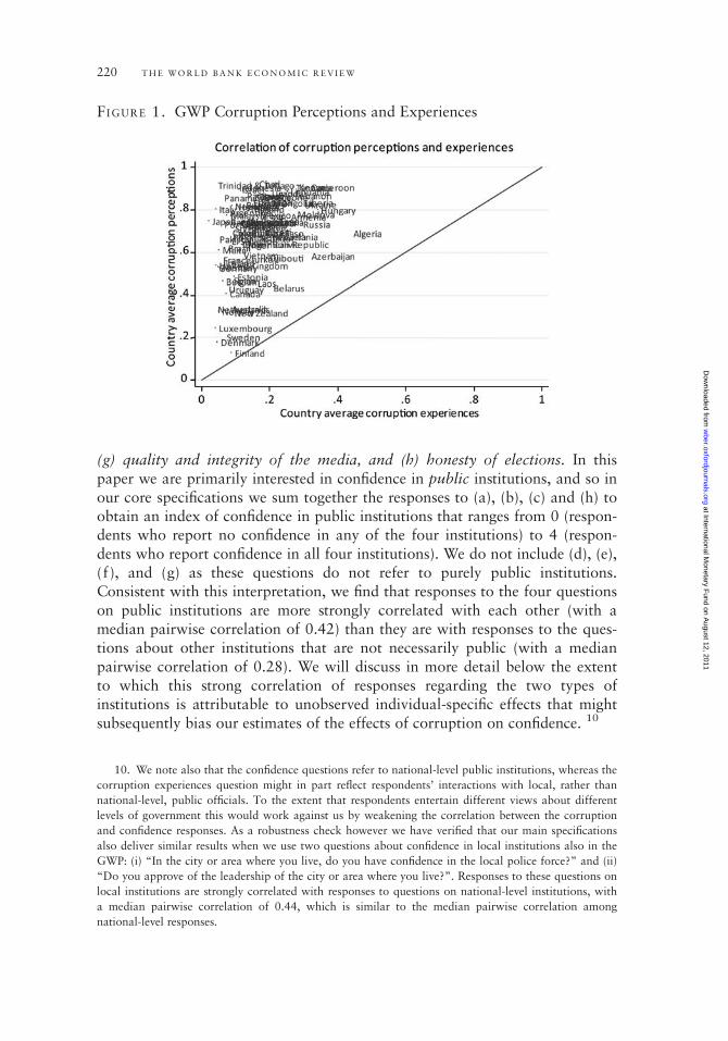
(g) quality and integrity of the media, and (h) honesty of elections. In thispaper we are primarily interested in confidence in public institutions, and so inour core specifications we sum together the responses to (a), (b), (c) and (h) toobtain an index of confidence in public institutions that ranges from 0 (respon-dents who report no confidence in any of the four institutions) to 4 (respon-dents who report confidence in all four institutions). We do not include (d), (e),(f ), and (g) as these questions do not refer to purely public institutions.Consistent with this interpretation, we find that responses to the four questionson public institutions are more strongly correlated with each other (with amedian pairwise correlation of 0.42) than they are with responses to the ques-tions about other institutions that are not necessarily public (with a medianpairwise correlation of 0.28). We will discuss in more detail below the extentto which this strong correlation of responses regarding the two types ofinstitutions is attributable to unobserved individual-specific effects that mightsubsequently bias our estimates of the effects of corruption on confidence. 10

FIGURE 1. GWP Corruption Perceptions and Experiences

10. We note also that the confidence questions refer to national-level public institutions, whereas the

corruption experiences question might in part reflect respondents’ interactions with local, rather than

national-level, public officials. To the extent that respondents entertain different views about different

levels of government this would work against us by weakening the correlation between the corruption

and confidence responses. As a robustness check however we have verified that our main specifications

also deliver similar results when we use two questions about confidence in local institutions also in the

GWP: (i) “In the city or area where you live, do you have confidence in the local police force?” and (ii)

“Do you approve of the leadership of the city or area where you live?”. Responses to these questions on

local institutions are strongly correlated with responses to questions on national-level institutions, with

a median pairwise correlation of 0.44, which is similar to the median pairwise correlation among

national-level responses.





Dow

nloaded from

Figure 3 documents how this measure of confidence in institutions fromthe GWP compares with the most closely-related variables on confidence ininstitutions taken from the World Values Survey.11 While the two measuresare highly correlated in the common sample of countries for which both

FIGURE 2. Correlation of GWP Corruption Experiences and PerceptionsQuestions with Worldwide Governance Indicators (WGI) ‘Control ofCorruption’ Variable

11. The WVS asks about respondents’ confidence in a variety of institutions. We aimed to match

this confidence index as closely as possible to our GWP index and therefore aggregated the answers to

the following four questions into an index ranging from 0 to 4: “I am going to name a number of

organizations. For each one, could you tell me how much confidence you have in them [. . .]: a) the

armed forces, b) the courts, c) the government (in your nation’s capital), d) parliament.”





Dow

nloaded from

measures are available (a correlation of 0.81), it is worth noting the signifi-cantly smaller country coverage of the WVS. The circles in the graph rep-resent countries that are present in our sample of the GWP but not in themost recent wave of the WVS. Using the GWP index therefore significantlyincreases the available cross-country sample to study effects of corruptionon confidence in institutions.

We note however that this very large increase in country coverage offered bythe GWP comes at the cost of a smaller number of respondents per country.Our sample size varies with availability of explanatory variables, but rangesfrom around 500 to 750 respondents per country, depending on the set of vari-ables considered. In contrast, the WVS survey used to construct Figure 3 fea-tures on average 1419 respondents per country. And the AfrobarometerSurveys used in several papers in this literature feature on average more than1000 respondents by country-year (see for example Table 4 in Lavallee,Razafindrakoto and Roubaud (2008)), although in a much smaller cross-section of just 18 countries in two waves).12

Finally, Figure 4 documents the relationship between the corruption ques-tions and the confidence in institutions index at the country level. The toppanel plots corruption perceptions against confidence in institutions and the

FIGURE 3. Comparing Confidence in Institutions: Country Average Values ofGWP and WVS Indices

12. A further distinction of the GWP relative to the Afrobarometer Surveys is that it provides

respondents only with binary response options to the corruption and confidence questions (Yes/No),

whereas the Afrobarometer Surveys offer more graduated responses (for example, “never”, “once or

twice”, “a few times”, or “often” are possible responses to the corruption experiences question). There

are advantages and disadvantages to both approaches. While the more graduated response in principle

offers more detail, this detail can be difficult to interpret absent clear evidence on how respondents

“anchor” the distinction between categories such as “a few times” and “once or twice”.





Dow

nloaded from

bottom panel plots corruption experiences against confidence. Both graphsdisplay a negative relationship between corruption and confidence althoughthis is much more pronounced for corruption perceptions. Here, all countrieswith very low average corruption perceptions score high on confidence ininstitutions. Scandinavian countries are the ones with the lowest perceivedcorruption and the highest confidence in institutions. Turning to corruptionexperiences, we see that in general countries with a higher share of people thathave experienced corruption report lower confidence in institutions. However,there are a number of countries that have low levels of experienced corruptionbut still report low confidence. In this group we find particularly LatinAmerican and Caribbean countries such as Panama, Argentina, Peru, andTrinidad and Tobago.

FIGURE 4. Confidence in Institutions and Corruption Experiences/Perceptions





Dow

nloaded from

I I I . M A I N R E S U L T S : R E S P O N D E N T - L E V E L E V I D E N C E

O N C O R R U P T I O N A N D C O N F I D E N C E I N I N S T I T U T I O N S

While the cross-country relationship between corruption and confidence in insti-tutions described above is suggestive of a link between the two, it is also farfrom convincing. A major concern here is that there may be many country-specific factors driving both variables. For example, some countries may simplyhave dysfunctional governments. On the one hand this will lead to high levels ofcorruption, and on the other hand public institutions naturally do not inspireconfidence in such an environment. Any correlation between our two variableswould simply reflect the omitted variable of government quality that is drivingboth corruption and confidence in public institutions. Another related possibilityhas to do with frame-of-reference issues in the survey responses themselves. It isplausible for example that citizens of rich countries have greater expectations ofthe quality and extent of public services provided by the government than docitizens in poor countries. In this case small departures from these high stan-dards might result in lower reported confidence in rich countries. Similarly theremight be greater tolerance of corruption in poor countries than in rich countries,resulting in lower reported corruption perceptions or experiences in poorcountries. Thus cross-country differences in expectations of corruption andpublic service quality might also spuriously contribute to the cross-country cor-relation between measured corruption and confidence.13

To address this first concern, we primarily focus on the respondent-levelvariation within countries to study the relationship between corruption andconfidence in institutions. Doing so allows us to control for any omittedcountry-level characteristics that might be driving the cross-country correlation.Table 1 documents the distinction between the within- and between-countryresults. Columns 1 and 3 reflect the between-country variation, showing coeffi-cients of cross-country linear regressions of confidence in institutions on thetwo corruption measures, using country-averaged data. In contrast columns2 and 4 capture the within-country variation, reporting estimates of the corre-sponding regressions including country fixed effects.14 In all cases we find anegative correlation between corruption and confidence in institutions that ishighly statistically significant. In the cross-country variation, the estimatedcoefficients imply that a one-standard-deviation increase (across countries) ineither of the two corruption measures reduces confidence in institutions by

13. A better approach to dealing with this problem of frame-of-reference issues is at the survey

design stage, for example through the introduction of anchoring vignettes to provide common context

to respondents’ qualitative responses. This option is unfortunately not available to us in the GWP which

did not field such vignettes.

14. It would technically be more appropriate to estimate an ordered probit model because of the

discrete and ordered nature of our dependent variable. Doing this does not change the sign or level of

significance of the coefficients. However, because of the difficulties involved with interpreting ordered

probit coefficients as marginal effects, we chose to present linear regression results throughout the paper.





Dow

nloaded from

between 0.2 and 0.3 points on a 0-4 scale.15 Within countries, the relationshipbetween corruption and confidence is also very strong. Here a one standarddeviation increases of either corruption variable within a country leads to areduction of confidence in institutions of between 0.1 and 0.3 points.16

Throughout the paper, we assess the significance of the within-country resultsusing standard errors that are clustered at the country level, and observationsare weighted using sampling weights provided by Gallup.

Anticipating our later discussion of endogeneity problems, we note that theestimated effect of the corruption perceptions question is nearly three times aslarge as the effect of the corruption experiences question. This is consistentwith our view that the former is much more likely to be endogenous to respon-dents’ confidence in public institutions, and that the latter much more plausiblyidentifies a causal effect running from corruption to confidence. While the esti-mated coefficients are statistically significant and quantitatively large, we notethat the explanatory power of corruption for the confidence question is limited.In particular, in the fixed-effects regressions, the bulk of the R-squared is dueto the country dummies. In contrast, the within R-squared net of the countryfixed effects is 0.01 for the corruption experiences question, and 0.06 for thecorruption perceptions question.

Although within-country regressions in Table 1 control for country-levelomitted variables, a possible objection is that there may also be a variety of

TA B L E 1. Bivariate Cross Country and Fixed Effects Regressions on theRelationship between Confidence in Institutions and Corruption

(1) (2) (3) (4)Confidence in

institutionsConfidence in


institutionsConfidence ininstitutions

cross-country fixed effects cross-country fixed effects

Corruption experiences -2.318*** -0.287***(-3.10) (-8.94)

Corruption perceptions -1.620*** -0.854***(-5.17) (-21.32)

_cons 2.118*** 2.904***(17.73) (13.15)

N 103 78063 103 78063No. of countries 103 103 103 103R-sq 0.098 0.230 0.233 0.271

Estimation in columns (1) and (3) is by ordinary least squares on country-level averages of allvariables, with heteroskedasticity-consistent standard errors. Estimation in columns (2) and (4) isby weighted least squares using sampling weights provided by Gallup, and heteroskedasiticity-consistent standard errors are clustered at the country level. T-statistics in parentheses:* p , 0.10, ** p , 0.05, *** p , 0.01

Source: Authors’ analysis with data from Gallup World Poll

15. Note that the cross-country standard deviations of corruption experiences and perceptions are

0.083 and 0.184, respectively.

16. Within-country standard deviation of corruption experiences is 0.360 and of corruption

perceptions 0.368.





Dow

nloaded from

individual-specific characteristics that influence both (i) respondents’ confidencein institutions; and (ii) the likelihood that they view corruption as prevalent, orthat they report having been solicited for a bribe.17 For example, richer, older,and more educated people might have more interactions with the state and sobe more likely to find themselves exposed to corruption, and might also bemore likely to have a cynical world view that precludes expressing confidencein public institutions.

To control for this we introduce a set of core control variables that we havefound to be correlated with the corruption questions, and that also tend to besignificant predictors of confidence in institutions. These include respondent age,gender, marital status, education, and the logarithm of self-reported income. Wealso introduce as basic control variables whether the household in which therespondent lives has access to the internet and a television. Access to such mediamay have ambiguous effects on individual’s opinions about and experienceswith corruption and institutions. On the one hand, officials might have a hardertime extracting bribes from more informed citizens that have had the chance toobtain information about laws and regulations concerning their dealings withgovernment. On the other hand, coverage of corruption cases in the mediamight influence corruption perceptions of individuals and may therefore have adirect effect on the answers to the perceptions question used in the GWP.

Table 2 presents the results adding these basic control variables. We notefirst that missing data presents a problem when introducing our set of corecontrol variables. In particular, data availability for education and income isincomplete, and this decreases our sample to about 57,000 individuals in94 countries. To aid in comparison with the previous results, we first repeatthe results with no controls from Table 1 in the smaller sample for which thecontrol variables are available, and then report results with controls. Reducingthe size of the sample in this way makes little difference for the effect ofcorruption on confidence in public institutions: the results without controlvariables in columns (1) and (3) of Table 2 are essentially identical to those incolumns (2) and (4) of Table 1. Second, we note that while the additionalcontrol variables featured in Table 2 do show some correlation with both the

17. Of course, controlling for country-level fixed effects will not address concerns about variations

in quality of subnational governments. It could for example be the case that within a country, some

local governments are corrupt and deliver low-quality public services, and as a result respondents have

low confidence in local government. It could then be that some of our observed within-country

correlation reflects heterogeneity in government performance across local governments. It is difficult to

control for this directly as the GWP does not contain much information attitudes towards local

governments. As an imperfect proxy for this, we average responses to the question “In the city or area

where you live, are you satisfied or dissatisfied with: (a) The public transporation systems, (b) the roads

and highways, and (c) the educational system or the schools. This question does clearly ask respondents

about public services in their locality, however it is not clear whether these are provided by local or by

national-level governments. Despite this ambiguity, we include this as a control variables (results not

reported but available from authors on request). Doing so has minimal effects on the size and

significance of our estimated effects of corruption on confidence. We are grateful to an anonymous

referee for pointing out this possible interpretation.





Dow

nloaded from

corruption and confidence variables, we find that the estimated coefficients onthe corruption variables change very little, declining just slightly in absolutevalue. Finally, we note that the control variables all enter with expected signsand are generally significant. Older individuals seem to have a lower degree ofconfidence in institutions although this relationship is not linear. Also, marriedrespondents express higher confidence than single ones. Higher income andeducation as well as access to internet and TV appear to reduce confidencealthough these latter effects are not statistically significant in all cases.

While the results in Table 2 are suggestive of a strong relationshipbetween confidence in institutions on the one hand, and corruption perceptionsand experiences on the other, one might nevertheless reasonably worry that thiscorrelation is driven by other unobserved respondent-specific characteristics.18

TA B L E 2. Fixed Effects Regressions Including Control Variables





institutions

Corruption experiences -0.298*** -0.282***(-7.73) (-7.41)

Corruption perceptions -0.870*** -0.865***(-20.71) (-20.54)

Male 0.00637 -0.00831(0.30) (-0.41)

Age -0.0167*** -0.0149***(-6.51) (-5.80)

Age2 0.000210*** 0.000190***(7.39) (6.69)

Married 0.0933*** 0.0775***(4.57) (3.76)

Secondary education -0.121*** -0.115***(-3.94) (-4.02)

Tertiary education -0.0853 -0.108**(-1.65) (-2.45)

Income -0.000873 -0.0104(-0.07) (-0.82)

Internet access -0.0437 -0.0600**(-1.38) (-2.08)

TV -0.0321 -0.0228(-0.66) (-0.48)

N 57095 57095 57095 57095No. of countries 94 94 94 94R-sq 0.226 0.230 0.271 0.275

Estimation is by weighted least squares using sampling weights provided by Gallup, andheteroskedasiticity-consistent standard errors are clustered at the country level. T-statistics inparentheses: * p , 0.10, ** p , 0.05, *** p , 0.01


18. Of course a preferred way of dealing with this type of heterogeneity is to identify our effects

using individual-level over time variation in responses to the corruption and confidence questions.

Unfortunately this option is not available to us in our single cross-section of countries and respondents.





Dow

nloaded from

A leading possibility is that, conditional on the basic control variables describedabove, some individuals may simply have a negative outlook or worldviewwhich makes them more likely to think that corruption is widespread, and at thesame time drives their lack of confidence in public institutions. Kaufmann andWei (2000) coin this as a "kvetch" effect, after the Yiddish word for habitualcomplaining. To the extent that this drives the observed correlation between cor-ruption and confidence in public institutions, we cannot interpret it as a causallink from the former to the latter.

At first glance, one might think that this potential problem of kvetch is lesssevere for the corruption experiences question than for the corruption percep-tions question. However, while the former ostensibly is an objective questionabout the respondent’s experience, there are nevertheless ways in which kvetchmight creep into responses to this question as well. First, respondents prone tokvetch might simply falsely claim that they had been solicited for a bribe. Theymight also be more likely to interpret ambiguous interactions with a public offi-cial as a request for a bribe. Therefore, respondents who in general tend to com-plain a lot might also be more likely to report interactions with public officialsas involving a request for a bribe. Second, the question about experiences withbribery follows a battery of other questions about corruption, one of which isthe corruption perceptions questions described above. It is possible that respon-dents prone to kvetch might want to reinforce their point of stating that govern-ment corruption is a problem by subsequently answering that they personallyhave found themselves in a bribe situation, even if this is not the case.

Our strategy for dealing with this potential problem is to introduce controlvariables that we think may be good proxies for the propensity to kvetch. Weconsider three sets of such proxies.19 The first set relies on questions in thesurvey that focus on individuals’ self-reported well-being. For example, theGWP asks respondents whether they are satisfied with their living standards,and which rung on the ladder of life that they find themselves. The GWP alsoasks respondents whether they have felt a variety of emotions such as worry,stress, or happiness in the previous day. These variables are plausibly correlatedwith individual respondents’ predisposition to complain. Second, the GWPasks respondents their opinions about a number of country-level variablesincluding whether the economy is doing well or poorly, whether the economicoutlook is favorable, and whether corruption is getting better or worse. Sinceour regressions include country fixed effects that soak up all national-level vari-ation, variation in individuals’ responses to these questions can be interpretedas capturing their idiosyncratic perceptions of the same national-level reality,and as such will also plausibly be correlated with kvetch.

As a final control for kvetch, we note that the battery of questions fromwhich our "confidence in institutions" variables are drawn includes a furtherquestion about confidence in religious organizations. It seems plausible to us

19. See Appendix Table A for a detailed description of the kvetch proxies and the specific GWP

questions used in their construction.





Dow

nloaded from

that corruption perceptions or experiences are likely to have little direct impacton confidence in religious organizations. However there might be an indirecteffect through kvetch: individuals more likely to complain in general might alsoreport less confidence in religious organizations purely because of their propen-sity to kvetch. This suggests using a kind of differencing strategy to control forkvetch. In particular, one might ask whether corruption reduces the difference inconfidence in public institutions and confidence in religious organizations.Alternatively and more flexibly, we can simply introduce confidence in religiousorganizations directly into our main specification as a control for kvetch.

Table 3 documents the results controlling for these proxies for kvetch. Sincenot all of the kvetch variables are available for all observations, our sampleshrinks further to 49,019 respondents in 90 countries. As in Table 2, we firstdocument that our main results with basic respondent-level controls do notchange as we move to this smaller sample (compare columns (1) and (3) inTables 2 and 3). More interesting is how our results on the effects of corruptionperceptions and experiences on confidence in institutions change when wecontrol for kvetch. We find that the estimated impact of corruption on confidencefalls by about 34 percent (for the corruption experiences question) and by 40percent (for the corruption perceptions question). This is a good indication thatkvetch effects are present in the data and are at least partially addressed by thecontrols that we introduce. Interestingly, while both the corruption perceptionsand corruption experiences questions might be subject to kvetch, we think it isplausible that kvetch effects are stronger for the former. The results in Table 3are consistent with this: the coefficient on the corruption perceptions falls rela-tively more after the introduction of the kvetch controls. We note also that thekvetch controls are all highly-significant predictors of the confidence responses,and collectively contribute to a substantial increase in the explanatory power ofthe regressions (the R-squared increases from 0.22 to 0.38 in the case of corrup-tion experiences, and from 0.27 to 0.39 in the case of corruption perceptions.However, even after introducing these very rigorous controls for kvetch, thenegative relationship between corruption and confidence remains highly signifi-cant and the magnitude of both corruption coefficients remains large.20

20. A closely-related interpretation of these results is that individuals vary in their extent of

“generalized trust”, which could be thought of as the opposite of ‘kvetch’. In the extreme, one could very

well interpret responses to the corruption perceptions question and responses to questions about confidence

in public institutions as both simply serving as proxies for individuals’ “generalized trust”. Our strategy for

dealing with this problem would be the same as our strategy for dealing with ‘kvetch’ as the two are quite

similar. The first is to introduce controls that might serve as proxies for ‘kvetch’ or “generalized trust”

(although we note that Newton and Norris (2000) examined the question if trust and confidence is a

feature of basic personality types but found little evidence to support this hypothesis.) In this respect our

strategy of controlling for confidence in non-public institutions is particularly helpful because it directly

controls for individuals’ confidence and focuses only on the differential degree of confidence in public

relative to non-public institutions. The second is to emphasize the corruption experiences question, which

as we have argued is less likely to be tainted by either “kvetch” or “generalized trust”.





Dow

nloaded from

TA B L E 3: Fixed Effects Regressions Controlling for Kvetch





institutions

Corruptionexperiences

20.280***(26.67)

20.185***(25.62)

Corruptionperceptions

20.873***(220.05)

20.518***(216.37)

Male 0.0123 20.00647 20.00512 20.0144(0.52) (20.34) (20.23) (20.78)

Age 20.0157*** 20.00135 20.0141*** 20.00118(25.90) (20.54) (25.21) (20.47)

Age2 0.000198*** 0.0000456* 0.000180*** 0.0000425(6.76) (1.66) (6.02) (1.53)

Married 0.0890*** 0.0399** 0.0739*** 0.0342*(4.05) (2.13) (3.37) (1.80)

Secondaryeducation

20.131*** 20.118*** 20.124*** 20.116***

(23.94) (24.79) (24.04) (24.81)Tertiary education 20.0822 20.0791* 20.102** 20.0916**

(21.49) (21.74) (22.18) (22.21)Income 20.000267 20.0470*** 20.00943 20.0488***

(20.02) (23.68) (20.68) (23.76)Internet access 20.0612* 20.0784*** 20.0817** 20.0872***

(21.71) (23.17) (22.55) (23.68)TV 20.0327 20.101*** 20.0234 20.0943**

(20.67) (22.86) (20.49) (22.62)Ladder of life 0.0151*** 0.0139**

(2.74) (2.61)Standard of living 0.228*** 0.220***

(8.30) (8.02)Emotions 0.0533*** 0.0519***

(4.90) (4.77)Economy good/bad 0.530*** 0.489***

(17.52) (17.20)Economic outlook 20.190*** 20.183***

(211.61) (211.70)Corruption trend 20.272*** 20.207***

(215.54) (212.61)Religious

organizations0.705*** 0.689***

(19.25) (18.81)N 49019 49019 49019 49019No. of countries 90 90 90 90R-sq 0.218 0.378 0.264 0.392

Estimation is by weighted least squares using sampling weights provided by Gallup, andheteroskedasiticity-consistent standard errors are clustered at the country level. T-statistics in par-entheses: * p , 0.10, ** p , 0.05, *** p , 0.01






Dow

nloaded from

I V. R O B U S T N E S S O F T H E M A I N R E S U L T S

Thus far we have seen that there is a large and statistically significant partialcorrelation between measures of corruption and confidence in public insti-tutions, and that this result is robust to the addition of (a) country fixedeffects, (b) a set of respondent-level controls, and (c) a set of proxies for‘kvetch’. In this section we subject these main results to a variety of furtherrobustness checks. We first disaggregate the confidence in institutions measureinto its four components and investigate how the effects of corruption varyacross these components. We then also estimate our main specificationcountry-by-country, and document how the estimated coefficients on thecorruption questions vary by country, by level of corruption, and by level ofdevelopment.

In Table 4 we disaggregate the confidence in institutions measure into itsfour components: confidence in the military, judiciary, national government,and in the honesty of elections. In the first four columns we report results forour core specification, using each of these components of the overall confidencemeasure separately as the dependent variable.21 We do this for both the corrup-tion experiences (top panel) and corruption perceptions measure (bottompanel). In all cases, we include, but do not report estimated coefficients for, thefull set of control variables used in Table 3. For the corruption experiencesquestion, we find only modest differences across components in terms of themagnitude of the estimated partial correlation between corruption and confi-dence. This effect is largest for confidence in the judiciary at 0.06, and smallestfor confidence in the honesty of elections, at 0.04. There is somewhat morevariation across the various confidence measures for the corruption perceptionsquestion. The estimated effect of corruption is much lower for confidence inthe military, at 0.06, than it is for the other three measures, which range from0.13 to 0.17.

Thus far we have assumed that the slope of the relationship between corrup-tion and confidence in public institutions is the same in all countries, at allincome levels, and at all levels of corruption. We now relax this assumptionand re-estimate our main specification from Table 3, country-by-country, sothat we can investigate how this slope varies across countries. We note firstthat the means of the country-by-country estimates in Table 5 are slightlysmaller than the pooled estimates in Table 3 (at -0.13 and -0.47 for the corrup-tion experiences and perceptions questions, respectively). The sign of the esti-mated coefficient is also fairly consistently negative across countries, with67 percent (91 percent) of country estimates being negative for the corruptionexperiences (perceptions) question. However, and not surprisingly, in many

21. Since the dependent variable for the individual confidence in institutions regressions is a binary

variable, a probit specification would be more appropriate than the linear probability model. However,

to improve comparability with previous results we report estimates from linear probability models here.

We have also estimated the specifications in Table 4 using a probit model and find a similar pattern of

relative magnitudes of the effect of corruption on the different confidence in institutions variables.





Dow

nloaded from

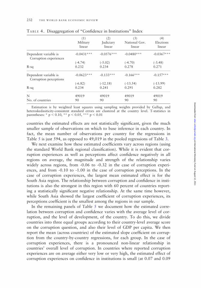
countries the estimated effects are not statistically significant, given the muchsmaller sample of observations on which to base inference in each country. Infact, the mean number of observations per country for the regressions inTable 5 is just 594, as opposed to 49,019 in the pooled regressions of Table 3.

We next examine how these estimated coefficients vary across regions (usingthe standard World Bank regional classification). While it is evident that cor-ruption experiences as well as perceptions affect confidence negatively in allregions on average, the magnitude and strength of the relationship varieswidely across regions, from -0.06 to -0.32 in the case of corruption experi-ences, and from -0.10 to -1.00 in the case of corruption perceptions. In thecase of corruption experiences, the largest mean estimated effect is for theSouth Asia region. The relationship between corruption and confidence in insti-tutions is also the strongest in this region with 60 percent of countries report-ing a statistically significant negative relationship. At the same time however,while South Asia showed the largest coefficient of corruption experiences, itsperceptions coefficient is the smallest among the regions in our sample.

In the remaining panels of Table 5 we document how the estimated corre-lation between corruption and confidence varies with the average level of cor-ruption, and the level of development, of the country. To do this, we dividecountries into three equal groups according to their country-level average scoreon the corruption question, and also their level of GDP per capita. We thenreport the mean (across countries) of the estimated slope coefficient on corrup-tion from the country-by-country regressions, for each group. In the case ofcorruption experiences, there is a pronounced non-linear relationship incountries’ overall level of corruption. In countries where reported corruptionexperiences are on average either very low or very high, the estimated effect ofcorruption experiences on confidence in institutions is small (at 0.07 and 0.09

TA B L E 4. Disaggregation of “Confidence in Institutions” Index

(1) (2) (3) (4)Military Judiciary National Gov. Electionslinear linear linear linear

Dependent variable isCorruption experiences

-0.0431*** -0.0576*** -0.0480*** -0.0367***

(-4.74) (-5.02) (-4.70) (-3.48)R-sq 0.232 0.234 0.278 0.271

Dependent variable isCorruption perceptions

-0.0623*** -0.133*** -0.166*** -0.157***

(-6.82) (-12.18) (-13.54) (-13.99)R-sq 0.234 0.241 0.291 0.282

N 49019 49019 49019 49019No. of countries 90 90 90 90

Estimation is by weighted least squares using sampling weights provided by Gallup, andheteroskedasiticity-consistent standard errors are clustered at the country level. T-statistics inparentheses: * p , 0.10, ** p , 0.05, *** p , 0.01





Dow

nloaded from

TA

BL

E5

.D

isaggre

gat

ion

into

Subgro

ups

Dep

endin

gon

Geo

graphic

Reg

ion,

Lev

elof

Corr

upti

on,

and

Inco

me

CO

RR

UPT

ION

EX

PE

RIE

NC

ES

CO

RR

UPT

ION

PE

RC

EPT

ION

S

No.

of

countr

ies

ingro

up

Mea

nes

tim

ated

slope

coef

fici

ent

Sta

ndard

dev

iati

on

of

slope

coef

fici

ent

Pro

port

ion

of

neg

ativ

eco

effici

ents

Pro

port

ion

of

neg

ativ

eand

signfica

nt

coef

fici

ents

*

Mea

nes

tim

ated

slope

coef

fici

ent

Sta

ndard

dev

iati

on

of

slope

coef

fici

ent

Pro

port

ion

of

neg

ativ

eco

effici

ents

Pro

port

ion

of

neg

ativ

eand

signfica

nt

coef

fici

ents

*

Full

sam

ple

90

-0.1

34

0.2

55

0.6

78

0.2

22

-0.4

66

0.3

76

0.9

11

0.6

33

Euro

pe

&

Cen

tral

Asi

a

11

-0.1

72

0.2

00

0.7

27

0.2

72

-0.3

12

0.4

19

0.8

18

0.4

54

Mid

dle

-East

&

Nort

hA

fric

a

4-0

.153

0.2

82

0.7

50

0.2

50

-0.7

30

0.2

50

1.0

00

1.0

00

East

Asi

a&

Pac

ific

9-0

.060

0.1

75

0.6

67

0.2

22

-0.2

24

0.2

97

0.7

78

0.3

33

South

Asi

a5

-0.3

19

0.2

65

0.8

00

0.6

00

-0.1

04

0.2

59

0.6

00

0.4

00

Lat

inA

mer

ica

&

Cari

bbea

n

19

-0.1

94

0.2

71

0.6

84

0.3

69

-0.4

90

0.1

91

1.0

00

0.7

37

Sub-S

ahara

n

Afr

ica

18

-0.0

61

0.2

78

0.6

11

0.2

22

-0.4

72

0.5

21

0.8

89

0.5

56

Hig

hin

com

e:

OE

CD

20

-0.1

13

0.2

81

0.6

50

0.0

00

-0.5

61

0.2

11

1.0

00

0.8

00

Hig

hin

com

e:

non-O

EC

D

4-0

.094

0.1

43

0.7

50

0.0

00

-1.0

06

0.3

85

1.0

00

0.7

50

Low

leve

lof

corr

upti

on

exper

ience

s/

per

cepti

ons

30

-0.0

66

0.2

41

0.6

00

0.0

00

-0.4

85

0.4

07

0.9

33

0.6

33

(Conti

nued

)





Dow

nloaded from

TA

BL

E5.

Conti

nued

CO

RR

UPT

ION

EX

PE

RIE

NC

ES

CO

RR

UPT

ION

PE

RC

EPT

ION

S

No.

of

countr

ies

ingro

up

Mea

nes

tim

ated

slope

coef

fici

ent

Sta

ndard

dev

iati

on

of

slope

coef

fici

ent

Pro

port

ion

of

neg

ativ

eco

effici

ents

Pro

port

ion

of

neg

ativ

eand

signfica

nt

coef

fici

ents

*

Mea

nes

tim

ated

slope

coef

fici

ent

Sta

ndard

dev

iati

on

of

slope

coef

fici

ent

Pro

port

ion

of

neg

ativ

eco

effici

ents

Pro

port

ion

of

neg

ativ

eand

signfica

nt

coef

fici

ents

*

Med

ium

leve

lof

corr

upti

on

exper

ience

s/

per

cepti

ons

30

-0.2

43

0.2

38

0.8

33

0.3

67

-0.4

47

0.3

45

0.8

67

0.6

67

Hig

hle

vel

of

corr

upti

on

exper

ience

s/

per

cepti

ons

30

-0.0

93

0.2

56

0.6

00

0.3

00

-0.4

65

0.3

84

0.9

33

0.6

00

Low

inco

me

30

-0.1

29

0.2

72

0.6

00

0.3

00

-0.3

70

0.4

37

0.8

67

0.4

00

Med

ium

inco

me

30

-0.1

53

0.2

44

0.7

33

0.3

00

-0.4

49

0.4

06

0.8

67

0.7

33

Hig

hin

com

e30

-0.1

21

0.2

56

0.7

00

0.0

67

-0.5

79

0.2

34

1.0

00

0.7

67

*st

atis

tica

lly

signifi

cant

coef

fici

ents

atat

least

the

5per

cent

leve

lw

ere

incl

uded

Eac

hro

wpro

vid

essu

mm

ary

stat

isti

cson

indic

ated

slope

coef

fici

ents

esti

mat

edco

untr

y-b

y-c

ountr

yw

ithin

the

indic

ated

countr

ygro

ups.

Countr

y-l

evel

esti

mat

ion

isby

wei

ghte

dle

ast

square

susi

ng

sam

pling

wei

ghts

pro

vid

edby

Gallup.





Dow

nloaded from

respectively). In contrast, for intermediate-corruption countries, the adverseeffect of corruption on confidence is much larger.

This suggests that in countries where corruption is rare, a respondent’s iso-lated experience with having been solicited for a bribe will not be enough to sub-stantially undermine his or her faith in overall public institutions. And similarly,in countries where corruption is widespread, personal experiences with or per-ceptions of corruption might also not change confidence in public institutionsbecause this confidence is very low to begin with. In contrast, for countries witha moderate prevalence of corruption, personal experiences with corruption havea stronger adverse impact on confidence in public institutions. Interestingly,however, this pattern is not present in the corruption perceptions question, noris it present when countries are divided into groups according to income levels.

V. C O N C E R N S A B O U T E N D O G E N E I T Y

We now discuss the extent to which the partial correlation between corruptionand confidence in public institutions can be interpreted as a causal effect from theformer to the latter. As noted in the introduction, there is an important identifi-cation problem: corruption might lead to a loss of confidence in public institutionsas we emphasize here, but at the same time, respondents who report low confi-dence in public institutions might as a result hold the belief that corruption iswidespread as well. This point is also noticed by Cho and Kirwin (2007) whoargue that individuals who do not trust public institutions might be more likely toresort to bribery to advance their interests, or to believe that corruption is wide-spread. This can lead to vicious circles where corruption and a lack of confidencein public institutions feed off each other. This potential for bi-directional causa-tion complicates the interpretation of the partial correlation between corruptionand confidence in institutions that we have documented. This is the classic identifi-cation problem: the observed correlation between corruption and confidencemight reflect causal effects from corruption to confidence that we emphasize. Butit could also reflect causation in the opposite direction.

We note first that a particular strength of the corruption experiences ques-tion is that it is much less likely to be prone to reverse causation than the cor-ruption perceptions question. To see why, recall that the experience questionasks respondents whether they have been solicited for a bribe during the past12 months. To the extent that the decision to solicit a bribe originates with thepublic official with whom the respondent is interacting, there should be no pro-blems of reverse causation: it seems unlikely that a public official would evenknow the respondent’s confidence in public institutions, let alone base hisdecision to solicit a bribe on it.22 This stands in contrast with the corruption

22. Indeed, the pattern of reverse causation might go against our results, if individuals with low

confidence in public institutions choose not to interact with government agencies and so are less likely

to report having been asked for a bribe.





Dow

nloaded from

perceptions question, where there is a more plausible channel of causation inthe opposite direction: individuals who have low confidence in public insti-tutions may precisely for this reason also believe that corruption is widespreadin government. This potential endogeneity bias may in part account for thefact that in most of our specifications thus far, the estimated slope of therelationship between corruption perceptions and confidence is larger in absol-ute value, and typically is also much more significant, than in the regressionsusing the corruption experiences question. Thus we argue that our results usingthe corruption experiences question provide a more plausible estimate of thecausal effect of corruption on confidence in public institutions than do ourresults with the corruption perceptions question.

At the same time, we acknowledge that there may still be such endogeneitybias, although to a lesser extent, even in the corruption experiences question.This would occur if respondents expressing a low confidence in public insti-tutions are more likely to interpret an ambiguous interaction with a public offi-cial as a request for a bribe than other respondents with higher confidence inpublic institutions. Such potential endogeneity bias is extremely difficult tocorrect using purely cross-sectional observational data such as what we have inthe GWP. This is because the usual strategy with observational data of identify-ing instruments (variables that plausibly affect only corruption, but not confi-dence in institutions, and vice versa) is very difficult to implement since it ishard to make a compelling case for the requisite exclusion restrictions.

In particular, we find it hard to make a convincing case that there are vari-ables in the GWP that predict corruption at the individual level, but do nothave direct predictive power for confidence in institutions, that we could thenuse as instruments for corruption. To illustrate why we think this approach isnot promising, consider the identifying assumptions implicit in the few papersin the literature that have attempted this instrumental variables strategy. Choand Kirwin (2007) make the identifying assumption that variables such asrespondents’ overall trust in others, and their perceptions of the political influ-ence of ethnic groups, matter only for corruption and have no direct effect onconfidence in institutions (see the exclusion restrictions implicit in theirTable 1). Lavallee, Razafindrakoto, and Roubaud (2008) claim with little justi-fication that a dummy variable indicating that the respondent is head of thehousehold, and a variable capturing the respondent’s views on the acceptabilityof paying a bribe, matter only for corruption and have no direct effect onconfidence.

We do not find such exclusion restrictions to be convincing. One mighteasily imagine that any of these variables are directly correlated with confi-dence in public institutions: for example respondents’ might believe that payinga bribe is acceptable precisely because they have no confidence in public insti-tutions. It is also striking that in both papers, the instrumented estimates of theeffects of corruption on confidence are vastly larger in absolute value than theuninstrumented estimates, while the feedback problem these authors seek to





Dow

nloaded from

correct would suggest that the true effects of corruption on confidence shouldbe much smaller in absolute value than the corresponding OLS estimates (seecolumns (1) and (2) of Table 1 in Cho and Kirwin (2007) and Table 4 inLavallee, Razafindrakoto and Roubaud (2008)). These counterintuitive resultslikely are due to a failure of the exclusion restrictions required to justify theinstrumental variables estimator.23 24 In contrast, we have consistently foundthat the magnitude of the effect of the more exogenous corruption experiencesquestion on confidence is always substantially smaller than the effect of thecorruption perceptions question, consistent with the view that the former isless tainted by reverse causation.

Absent compelling instruments, we use an argument based on Leamer(1981) to provide a rough bound on the extent to which our estimates mightreflect reverse causation. To make this concrete let y denote the portion of con-fidence that is orthogonal to all of the control variables, including the countryfixed effects, in columns 2 and 4 of Table 3, and let x denote the same orthog-onal component of corruption. The possibility of causal effects in both direc-tions between corruption and confidence can be captured by the assumptionthat y and x are generated by the following system of two equations:

y ¼ bxþ 1

x ¼ gyþ yð1Þ

We are primarily interested in the slope coefficient b which captures the effectof corruption on confidence. However, we cannot identify this effect absentsome instrument that shifts corruption without at the same time affecting confi-dence, i.e. we need to find a variable that is included in the second equationbut excluded from the first.

Absent such an instrument, the problem is simply that there are fourunknown parameters in this system (b, g, and the two variances of the errorterms), while there are just three moments in the data (V(x), V(y), andCOV(x,y)).25 However, we can still make progress by exploring how our

23. Lavallee, Razafindrakoto and Robaud (2008) claim support for their identification strategy in

the fact that tests of overidentifying restrictions fail to reject the null of instrument validity. Here they

fall into the (unfortunately common) pitfall of failing to recognize that such tests are valid only if at

least one instrument is indeed valid. We think it is very difficult to make such a case even for just one

instrument in this context.

24. An alternative approach sometimes used with survey data is to use the average of the corruption

question across all observations within a pre-specified group, for example all respondents in the same

city, as an instrument for corruption. This is plausible as an identification strategy only to the extent

that we think that the unexplained portion of confidence is uncorrelated across respondents within a

group. This assumption is difficult to justify in practice.

25. In fact things might be even more complicated, as we have assumed for simplicity that the

covariance between the two structural errors is zero as well. We justify this simplifying assumption by

observing that in Table 3 we have already controlled for a large set of variables that might

simultaneously be driving corruption and confidence. Thus it is more plausible that the errors in the

orthogonalized system here are independent.





Dow

nloaded from

estimate of b would change given differing assumptions on the strength of thereverse causation captured by g. To do this, express the three observable datamoments in terms of the four unknown parameters, and then solve for b con-ditional on a value of g. Then by varying g we can explore the robustness ofour conclusions about b to alternative assumptions regarding the strength ofthe reverse causation. Some simple algebra delivers this very natural estimatorfor b as a function of g:

b ¼ COVðx; yÞ � gVðyÞVðxÞ � gCOVðx; yÞ ð2Þ

Note that when g ¼ 0 we retrieve the OLS estimator, i.e.b ¼ COVðx; yÞ=VðxÞ, since in this case there is no feedback from confidenceto corruption, and so OLS is valid. On the other hand, note that b ¼ 0 wheng ¼ COV(x,y)/V(y) which is simply the OLS estimate of the feedback effect inthe second equation. This is because if there is in fact no causal effect runningfrom corruption to confidence, then the second equation can be estimated byOLS.26 Moreover, the range from g ¼ 0 to g ¼ COV(x,y)/V(y) seems to us tobe a reasonable prior bound for the magnitude of reverse causation. It seemsreasonable to assume that g , 0, i.e. less confidence implies more corruption.However, the magnitude of this effect is likely to be less (in absolute value)than g ¼ COV(x,y)/V(y). If it were not, then the data would imply that b . 0,i.e. that corruption raises confidence in public institutions, which seemsimplausible.

We plot this estimate of b (on the vertical axis) as a function of g (on thehorizontal axis) in Figure 5, using this prior plausible range of values for themagnitude of reverse causation. The top panel refers to the corruption experi-ences question, and the bottom to the corruption perceptions question. In bothpanels, when g ¼ 0 we retrieve the OLS estimates of b on the horizontal axiscorresponding to those in Columns (2) and (4) of Table 3. As we allow for thepossibility of more and more reverse causation, i.e. as g becomes more andmore negative capturing a stronger effect of confidence on corruption, our esti-mate of the main effect of interest, b, becomes closer and closer to zero. Wealso report 95 percent confidence intervals for b, and these suggest that ourestimate of b would be insignificantly different from zero only if g were very

26. While rarely used, it is interesting to note that the basic argument here is nearly 80 years old!

Leamer (1981) credits Leontief (1929) with first performing this basic calculation. A very recent and

growing literature on instrumental variables estimation with imperfect instruments can be thought of as

resurrecting some of these basic insights as well (see for example Kraay (forthcoming), Conley, Hansen

and Rossi (forthcoming), and Nevo and Rosen (forthcoming). In the case of OLS which we consider

here where the corruption variable serves as its own instrument, the unobserved feedback parameter g

governs the strength of the correlation between the instrument and the error term. The approaches in

these three more recent papers can be thought of as a more formal way of exploring how the IV

estimator varies with alternative assumptions about the strength of the correlations of the instrument

with the error term.





Dow

nloaded from

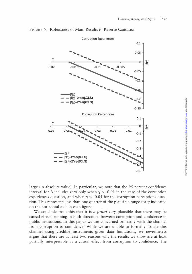
large (in absolute value). In particular, we note that the 95 percent confidenceinterval for b includes zero only when g , -0.01 in the case of the corruptionexperiences question, and when g , -0.04 for the corruption perceptions ques-tion. This represents less than one-quarter of the plausible range for g indicatedon the horizontal axis in each figure.

We conclude from this that it is a priori very plausible that there may becausal effects running in both directions between corruption and confidence inpublic institutions. In this paper we are concerned primarily with the channelfrom corruption to confidence. While we are unable to formally isolate thischannel using credible instruments given data limitations, we neverthelessargue that there are at least two reasons why the results we show are at leastpartially interpretable as a causal effect from corruption to confidence. The

FIGURE 5. Robustness of Main Results to Reverse Causation





Dow

nloaded from

first is that, as we have discussed, it is much more difficult to see the channelfor potential reverse causation in the results using the corruption experiencesquestion. The second is that, even if reverse causation were present, it wouldneed to be extremely strong in order to undermine our conclusion of a statisti-cally significant effect of corruption on confidence.

V I . W H Y D O E S T H E A D V E R S E E F F E C T O F C O R R U P T I O N

O N C O N F I D E N C E I N I N S T I T U T I O N S M A T T E R ?

Thus far we have documented a strong negative relationship between corrup-tion and confidence in public institutions. We conclude by using a smallnumber of variables available in the GWP to investigate some direct conse-quences of this loss of confidence. We do so in an effort to shed some light onwhat might be some of the mechanisms through which corruption-inducedlack of confidence in public institutions could undermine the functioning ofthose institutions. In particular, we find some evidence that reduced confidencein public institutions leads to a reduction in political participation, raisessupport for violent means of political expression, and increases the desire ofrespondents to vote with their feet through emigratation. We interpret each ofthese as a signal of respondents’ likelihood to “opt out” of participation inpublic institutions in a country. This in turn is suggestive of how lack of confi-dence in public institutions undermines their effectiveness, but it is of coursefar from the final word.

We draw on a number of questions from the GWP to measure these conse-quences of corruption-induced losses in confidence. To measure political par-ticipation, we use the GWP question which asks “In the past month, have youvoiced your opinion to a public official?" As a measure of support for violentforms of protest, we use a question from the GWP which asks: “Do you thinkgroups that are oppressed and are suffering from injustice can improve theirsituation by peaceful means alone?” And finally, the desire to emigrate iscaptured by response to the question "Ideally, if you had the opportunity,would you like to move permanently to another country, or would you preferto continue living in this country?"

In Table 6 we document the relationship between corruption, confidence,and these three outcomes. In the first column, we report the simple bivariaterelationship between the confidence variable and the three outcome variablesof interest, and in the second column we introduce the full set of control vari-ables from Table 3. We find strong evidence that a lack of confidence in publicinstitutions raises sympathy for violent protest, raises the desire to migrate, andreduces political participation. We next investigate the extent to which thisreflects the effect of corruption perceptions and corruption experiences. Incolumns three and four we estimate regressions of the three outcome variableson the two corruption variables alone (but still controlling for the full set ofcontrol variables from Table 3). Here we find evidence that those individuals





Dow

nloaded from

TA

BL

E6

.W

hy

Do

Adve

rse

Eff

ects

of

Corr

upti

on

Mat

ter?

(1)

(2)

(3)

(4)

(5)

(6)

Ach

ieve

change

by

pea

cefu

lm

eans

Ach

ieve

change

by

pea

cefu

lm

eans

Ach

ieve

change

by

pea

cefu

lm

eans

Ach

ieve

change

by

pea

cefu

lm

eans

Ach

ieve

change

by

pea

cefu

lm

eans

Ach

ieve

change

by

pea

cefu

lm

eans

Confiden

cein

inst

ituti

ons

0.0

958***

0.0

776***

0.0

764***

0.0

767***

(8.7

0)

(6.4

8)

(6.4

1)

(6.6

1)

Corr

upti

on

exper

ience

s2

0.0

833***

20.0

690**

(22.8

4)

(22.4

5)

Corr

upti

on

per

cepti

ons

20.0

572*

20.0

174

(21.7

6)

(20.5

8)

N46249

46249

46249

46249

46249

46249

No.

of

countr

ies

89

89

89

89

89

89

Contr

ols

no

yes

yes

yes

yes

yes

(1)

(2)

(3)

(4)

(5)

(6)

Lik

eto

move

tooth

erco

untr

y?

Lik

eto

move

tooth

erco

untr

y?

Lik

eto

move

tooth

erco

untr

y?

Lik

eto

move

tooth

erco

untr

y?

Lik

eto

move

tooth

erco

untr

y?

Lik

eto

move

tooth

erco

untr

y?

Confiden

cein

inst

ituti

ons

20.1

27***

20.0

676***

20.0

629***

20.0

622***

(28.4

5)

(24.6

3)

(24.2

7)

(24.2

6)

Corr

upti

on

exper

ience

s0.2

49***

0.2

36***

(7.1

5)

(6.6

3)

Corr

upti

on

per

cepti

ons

0.1

30***

0.0

964***

(4.3

5)

(3.2

2)

N34184

34184

34184

34184

34184

34184

(Conti

nued

)





Dow

nloaded from

TA

BL

E6.

Conti

nued

(1)

(2)

(3)

(4)

(5)

(6)

Ach

ieve

change

by

pea

cefu

lm

eans

Ach

ieve

change

by

pea

cefu

lm

eans

Ach

ieve

change

by

pea

cefu

lm

eans

Ach

ieve

change

by

pea

cefu

lm

eans

Ach

ieve

change

by

pea

cefu

lm

eans

Ach

ieve

change

by

pea

cefu

lm

eans

No.

of

countr

ies

69

69

69

69

69

69

Contr

ols

no

yes

yes

yes

yes

yes

(1)

(2)

(3)

(4)

(5)

(6)

Voic

edopin

ion

tooffi

cial

Voic

edopin

ion

tooffi

cial

Voic

edopin

ion

tooffi

cial

Voic

edopin

ion

tooffi

cial

Voic

edopin

ion

tooffi

cial

Voic

edopin

ion

tooffi

cial

Confiden

cein

inst

ituti

ons

0.0

259***

0.0

127

0.0

183*

0.0

127

(4.2

5)

(1.2

6)

(1.8

0)

(1.2

5)

Corr

upti

on

exper

ience

s0.3

01***

0.3

05***

(9.0

0)

(9.0

9)

Corr

upti

on

per

cepti

ons

20.0

0537

0.0

0135

(20.1

9)

(0.0

5)

N48774

48774

48774

48774

48774

48774

No.

of

countr

ies

90

90

90

90

90

90

Contr

ols

no

yes

yes

yes

yes

yes

Est

imat

ion

isby

wei

ghte

dle

ast

square

susi

ng

sam

pling

wei

ghts

pro

vid

edby

Gallup,

and

het

erosk

edasi

tici

ty-c

onsi

sten

tst

andard

erro

rsare

clust

ered

atth

eco

untr

yle

vel.

T-s

tati

stic

sin

pare

nth

eses

:*

p,

0.1

0,

**

p,

0.0

5,

***

p,

0.0

1





Dow

nloaded from

who have experienced corruption or who perceive corruption to be high intheir country show support for violent protest and express increased desire topermanently leave their country. In contrast however, having had a corruptionexperience raises the likelihood of individuals voicing their opinion to publicofficials. While the GWP does not ask about the nature of this interaction witha public official, it is possible that this positive correlation reflects preciselyrespondents complaining to public officials about their experience withcorruption.

Finally, we introduce both corruption measures together with confidence ininstitutions as explanatory variables. Doing so sheds light on whether theeffects of corruption on these outcomes operate only through confidence ininstitutions (in which case the corruption variables would not enter signifi-cantly), or whether there are direct effects of corruption (in which case theywould enter significantly even after controlling for confidence in public insti-tutions). In the case of corruption experiences, there seems to be fairly clearevidence of both direct and indirect effects, as both the corruption and confi-dence variables enter significantly. In the case of corruption perceptionshowever we find evidence of a direct effect only for the emigration question.Overall these findings provide some support to the findings of Putnam (2000)and Uslaner (2002) that institutional trust contributes to citizen’s involvementin the political process.

V I I . C O N C L U S I O N S

In this paper we have used data from the Gallup World Poll, a unique and verylarge global household survey, to document a quantitatively large and statisti-cally significant negative effect of corruption on confidence in public insti-tutions. This highlights an important, but relatively under-examined, channelthrough which corruption can inhibit development. Our findings are robust tothe inclusion of a large set of controls for country and respondent-level charac-teristics. In addition to considering a much larger sample of countries and amore thorough set of control variables, our main contribution relative to theexisting literature is our treatment of potential endogeneity biases. We haveargued that a key advantage of specific experiential questions about corruptionis that they are much more plausibly exogenous to respondents’ reported confi-dence in public institutions. As a result, the partial correlation between suchquestions and confidence can much more plausibly be interpreted as a causaleffect from the former to the latter.





Dow

nloaded from

AP P E N D I X TA B L E A. Variable Descriptions

Variable Wording of Question in GWP Definition

Confidence ininstitutions

Index composed of four subcategories of this question:"In this country, do you have confidence in each ofthe following, or not? How about the military?Judicial system and courts? National government?Honesty of elections?"

scale of 0 to 4 with 4indicating highestconfidence

Corruptionexperiences

"Sometimes people have to give a bribe or a present inorder to solve their problems. In the last 12 months,were you, personally, faced with this kind ofsituation, or not (regardless of whether you have thebribe/present or not)?"

dummy: 1 indicatingexposure to bribery

Corruptionperceptions

"Is corruption widespread throughout the governmentin this country, or not?"

dummy: 1 indicatingcorruption iswidespread

Male Share of malerespondents

Age Age in yearsMarried "What is your current marital status?"; responses of

"married" as well as "domestic partner" wereaggregated to form the "Married" variable

dummy: 1 indicatingmarried/domesticpartner

Secondaryeducation

"What is your highest level of education?" dummy: 1 indicatinghighest level istertiary education

Tertiaryeducation

"What is your highest level of education?" dummy: 1 indicatinghighest level issecondary education

Income "What is your total monthly household income, beforetaxes? Please include income from wages andsalaries, remittances from family member livingelsewhere, farming and all other sources."

Income in US dollars

Internet access "Does your home have access to the internet?" dummy: 1 indicatingyes

TV "Does your home have a television?" dummy: 1 indicatingyes

Ladder of life “Imagine a ladder numbered from zero at the bottomto ten at the top. Suppose we say that the top of theladder represents the best possible life for you, andthe bottom of the ladder represents the worstpossible life for you. On which step of the ladderwould you say you personally feel you stand at thistime, assuming that the higher the step the betteryou feel about your life, and the lower the step theworse you feel about it? Which step comes closest tothe way you fell?"

scale of 0 to 10 with10 being best life

Standard ofliving

“Are you satisfied or dissatisfied with your standard ofliving, all the things you can buy and do?”.

(0 or 1) with 1indicating satisfied

(Continued)





Dow

nloaded from

APPENDIX TABLE A. Continued

Variable Wording of Question in GWP Definition

Emotions Index composed of three subcategories of this question:“Did you experience the following feelings during alot of the day yesterday? How about Worry? Stress?Happiness?”

scale of 0 to 3 with 3indicating yes to all3 questions

Economy good/bad

"Do you believe the current economic conditions inthis country are good, or not?"

dummy: 1 indicatinggood

Economicoutlook

"Right now, do you think the economic conditions inthis country as a whole, are getting better or gettingworse?"

dummy: 1 indicatingbetter

Corruptiontrend

"Do you think the level of corruption in this country islower, about the same, or higher than it was 5 yearsago?"

dummy: 1 indicatingcorruption is higher

Religiousorganizations

"In this country, do you have confidence in each of thefollowing, or not? How about religiousorganizations (churches, mosques, temples etc.)?"

dummy: 1 indicatingconfidence

Voiced opinionto publicofficial

"Have you done any of the following in the pastmonth? How about voiced your opinion to a publicofficial?"

dummy: 1 indicating"yes"

Achieve changeby peacefulmeans

"Some people believe that groups that are oppressedand are suffering from injustice can improve theirsituations by peaceful means alone. Other do notbelieve that peaceful means alone will work toimprove the situation for such oppressed groups.Which do you believe?"

dummy: 1 indicating"peaceful meansalone will work"

Like to move toother country

"Ideally, if you had the opportunity, would you like tomove permanently to another country, or would youprefer to continue living in this country?"

dummy: 1 indicating"would like tomove"





Dow

nloaded from

AP

PE

ND

IXT

AB

LE

B.

Countr

ies

inC

ore

Sam

ple

by

Geo

graphic

al

Reg

ion

Euro

pe

&C

entr

al

Asi

aE

ast

Asi

a&

Pac

ific

South

Asi

aL

atin

Am

eric

a&

Cari

bbea

nSub-S

ahara

nA

fric

aM

iddle

-East

&N

ort

hA

fric

aH

igh

inco

me:

OE

CD

Hig

hin

com

e:non-O

EC

D

Arm

enia

Cam

bodia

Bangla

des

hA

rgen

tina

Bots

wana

Alg

eria

Aust

ralia

Est

onia

Aze

rbaijan

Indones

iaIn

dia

Bolivia

Burk

ina

Faso

Djibouti

Aust

ria

Isra

elB

elaru

sL

aos

Nep

al

Bra

zil

Buru

ndi

Iran

Bel

giu

mM

alt

aH

ungary

Mala

ysia

Pakis

tan

Chile

Cam

eroon

Leb

anon

Canada

Tri

nid

ad

&T

obago

Lat

via

Mongoli

aSri

Lanka

Colo

mbia

Chad

Den

mark

Lit

huania

Phil

ippin

esC

ost

aR

ica

Eth

iopia

Fin

land

Mold

ova

Taiw

an

Dom

inic

an

Rep

.G

hana

Fra

nce

Pola

nd

Thail

and

Ecu

ador

Ken

yaG

erm

any

Russ

iaV

ietn

am

El

Salv

ador

Lib

eria

Irel

and

Turk

eyG

uat

emala

Madagasc

ar

Italy

Ukra

ine

Hait

iM

auri

tania

Japan

Hondura

sN

iger

Luxem

bourg

Mex

ico

Sen

egal

Net

her

lands

Nic

ara

gua

Sie

rra

Leo

ne

New

Zea

land

Panam

aT

anza

nia

Norw

ayPara

guay

Togo

Port

ugal

Per

uU

ganda

South

Kore

aU

ruguay

Zam

bia

Spain

Ven

ezuel

aSw

eden

Unit

edK

ingdom





Dow

nloaded from

RE F E R E N C E S

Acemoglu, Daron, Simon Johnson, and James A. Robinson 2001. “The Colonial Origins of

Comparative Development: An Empirical Investigation.” American Economic Review, 91(5),

1369–1401.

Anderson, Christopher J., and Yuliya V. Tverdova 2003. “Corruption, Political Allegiances, and

Attitudes toward Government in Contemporary Democracies.” American Journal of Political

Science, 47(1), 91–109.

Azfar, Omar, and Peter Murrell 2009. Identifying Reticent Respondents: Assessing the Quality of

Survey Data on Corruption and Values, Economic Development and Cultural Change, University of

Chicago Press, Vol. 57(2), 387–411.

Bratton, Michael 2007. Are You Being Served? Popular Satisfaction with Health and Education Services

in Africa, Afrobarometer, Working Paper No. 65.

Catterberg, Gabriela, and Alejandro Moreno 2005. “The Individual Bases of Political Trust: Trends in

New and Established Democracies.” International Journal of Public Opinion Research, 18(1),

408–443.

Chang, Eric C.C., and Yun-han Chu 2006. “Corruption and Trust: Exceptionalism in Asian

Democracies?.” The Journal of Politics, 68(2), 259–271.

Cho, Wonbin, and Matthew F. Kirwin 2007. A Vicious Cycle of Corruption and Mistrust in Institutions

in Sub-Saharan Africa: A Micro-Level Analysis, Afrobarometer Working Paper, No. 71, Michigan

State University.

Clausen, Bianca, Aart Kraay, and Peter Murrell 2010. Does Respondent Reticence Affect the Results of

Corruption Surveys? Evidence from the World Bank Enterprise Survey for Nigeria. World Bank

Policy Research Department Working Paper No. 5415.

Conley, Timothy, Christian Hansen, and Peter Rossi forthcoming. “Plausibly Exogenous.” Review of

Economics and Statistics.

Deaton, Angus 2008. “Income, Health, and Wellbeing Around the World: Evidence from the Gallup

World Poll.” Journal of Economic Perspectives, 22(2), 53–72.

——— 2009. Aging, Religion, and Health, National Bureau of Economic Research Working Paper No.

15271.

Deaton, Angus, Jane Fortson, and Robert Tortora 2009. Life (Evaluation), HIV/AIDS, and Death in

Africa, National Bureau of Economic Research Working Paper No. 14637.

Della Porta, Donatella 2000. “Social Capital, Beliefs in Government, and Political Corruption,” in

Susan J. Pharr, and Robert D. Putnam eds.: Disaffected Democracies: What’s Troubling the

Trilateral Countries?, Princeton, NJ: Princeton University Press.

Easton, David 1965. A Systems Analysis of Political Life, New York: John Wiley.

——— 1975. “A Re-Assessment of the Concept of Political Support.” British Journal of Political

Science, 5(4), 435–457.

Gandelman, Nestor, and Ruben Hernandez-Murillo 2009. “The Impact of Inflation and Unemployment

on Subjective Personal and Country Evaluations.” Federal Reserve Bank of St. Louis Review, 91(3),

107–126.

Gibson, James L., and Gregory A. Caldeira 1995. “The Legitimacy of Transnational Legal Institutions:

Compliance, Support, and the European Court of Justice.” American Journal of Political Science,

39(2), 459–89.

Gibson, James L., Gregory A. Caldeira, and Lester K. Spence 2003. “Measuring Attitudes toward the

United States Supreme Court.” American Journal of Political Science, 39(2), 354–367.

Helliwell, John F. 2008. Life Satisfaction and Quality of Development, National Bureau of Economic

Research Working Paper No. 14507.





Dow

nloaded from

Helliwell, John F., Christopher P. Barrington-Leigh, Anthony Harris, and Haifang Huang 2009.

International Evidence on the Social Context of Well-Being, National Bureau of Economic Research

Working Paper No. 14720.

Hellman, Joel, and Daniel Kaufmann 2004. “The Inequality of Influence”. Available at SSRN: http

://ssrn.com/abstract=386901 or doi:10.2139/ssrn.386901.

Kaufmann, Daniel, Aart Kraay, and Massimo Mastruzzi 1999. Governance Matters, World Bank Policy

Research Department Working Paper No. 2196.

Kaufmann, Daniel, and Shang-Jin Wei 2000. “Does “Grease Money” Speed Up the Wheels of

Commerce?.” IMF Working Papers, 00/64, Washington DC: International Monetary Fund.

Kaufmann, Daniel, Aart Kraay, and Massimo Mastruzzi 2008. “Governance Matters VII: Aggregate

and Individual Governance Indicators 1996-2007.” Policy Research Working Paper, 4654,

Washington DC: The World Bank.

Kaufmann, Daniel, and Joel Hellman 2004. “Political Inequality and the Subversion of Institutions in

Transition Economies”, in Janos Kornai, and Susan Rose-Ackerman (eds). “Building a Trustworthy

State in Post-Socialist Transition”, Palgrave-MacMillan.

Knack, Stephen, and Philip Keefer 1995. “Institutions and Economic Performance: Cross-Country Tests

Using Alternative Institutional Measures.” Economics and Politics, 7(3), 207–227.

——— 1997. “Why Don’t Poor Countries Catch Up? A Cross-National Test for an Institutional

Explanation.” Economic Inquiry, 35(3), 590–602.

Kraay, Aart forthcoming. “Instrumental Variables Estimation with Uncertain Exclusion Restrictions: A

Bayesian Approach.” Journal of Applied Econometrics.

Krueger, Alan B., and Jitka Maleckova 2009. “Attitudes and Action: Public Opinion and the

Occurrence of International Terrorism.” Science, 235, 1534–1536.

Lambsdorff, Johann Graf 2007. The Institutional Economics of Corruption and Reform: Theory,

Evidence, and Policy, Cambridge: Cambridge University Press.

Lavallee, Emmanuelle, Mireille Razafindrakoto, and Francois Roubaud 2008: Corruption and Trust in

Political Institutions in Sub-Saharan Africa, Afrobarometer, Working Paper No. 102.

Leamer, Edward E. 1981. “Is it A Supply Curve or Is it a Demand Curve? Partial Identification

Through Inequality Constraints.” Review of Economics and Statistics, 63(3), 319–327.

Leontief, Wassily 1929. “Ein Versuch Zur Statistischen Analyse von Angebot und Nachfrage (An

Inquiry on the Statistical Analysis of Supply and Demand).” Weltwirtschaftliches Archiv, 30(1),

1–53.

Mauro, Paolo 1995. “Corruption and Growth.” The Quarterly Journal of Economics, 110(3),

681–712.

Meon, Pierre-Guillaume, and Khalid Sekkat 2004. “Does the Quality of Institutions Limit the MENA’s

Integration in the World Economy.” The World Economy, 27(9), 1475–1498.

Meon, Pierre-Guillaume, and Khalid Sekkat 2005. “Does Corruption Grease or Sand the Wheels of

Growth?.” Public Choice, 122(1), 69–79.

Mishler, William, and Richard Rose 2001. “What are the Origins of Political Trust? Testing

Institutional and Cultural Theories in Post-Communist Societies.” Comparative Political Studies,

Vol. 34(1), 30–62.

——— 2005. “What Are the Consequences of Trust? A Test of Cultural and Institutional Theories in

Russia.” Comparative Political Studies, 38(9), 1050–1078.

Mo, Pak Hung 2001. “Corruption and Growth.” Journal of Comparative Economics, 29(1), 66–79.

Nevo, Aviv, and Adam Rosen forthcoming. “Inference with Imperfect Instrumental Variables.” Review

of Economics and Statistics.

Newton, Kenneth, and Pippa Norris 2000. “Confidence in Public Institutions: Faith, Culture, or

Performance?,” in Susan J. Pharr, and Robert D. Putnam: Disaffected Democracies: What’s

Troubling the Trilateral Economies, Princeton, NJ: Princeton University Press.





Dow

nloaded from

Ng, Weiting, Ed Diener, Raksha Aurora, and James Harter 2008. “Affluence, Feelings of Stress, and

Well-Being.” Social Indicators Research, doi:10.1007/s11205-008-9422-5.

North, Douglass C. 1990. Institutions, Institutional Change, and Economic Performance, New York:

Cambridge University Press.

Pelham, Brett, Steve Crabtree, and Zsolt Nyiri 2009. “Technology and Education.” Harvard

International Review, Summer, 74–76.

Pellegrini, Lorenzo, and Reyer Gerlagh 2004. “Corruption’s Effects on Growth and its Transmission

Channels.” Kyklos, 57(3), 429–456.

Pharr, Susan 2000. “Officials’ Misconduct and Public Distrust: Japan and the Trilateral Democracies,“

in Susan J. Pharr, and Robert D. Putnam eds.: Disaffected Democracies: What’s Troubling the

Trilateral Countries?, Princeton, NJ: Princeton University Press.

Putnam, Robert D. 2000. Bowling Alone, New York: Simon & Schuster.

Rodrik, Dani, Arvind Subramanian, and Francesco Trebbi 2004. “Institutions Rule: The Primacy of

Institutions over Geography and Integration in Economic Development.” Journal of Economic

Growth, 9(2), 131–165.

Rose, Richard, William Mishler, and Christian Haerpfer 1998. Democracy and its Alternatives:

Understanding Postcommunist Societies, Baltimore: The Johns Hopkins University Press.

Sacks, Audrey 2011. “The Antecedents of Approval of the Incumbent Government and Trust in

Government in sub-Saharan Africa, Latin America, and Six Arab Countries”. Manuscript, the World

Bank Institute.

Seligson, Mitchell A. 2002. “The Impact of Corruption on Regime Legitimacy: A Comparative Study of

Four Latin American Countries.” The Journal of Politics, 64(2), 408–433.

Stevenson, Betsey, and Justin Wolfers 2008. “Economic Growth and Subjective Well-Being: Reassessing

the Easterlin Paradox.” Brookings Papers on Economic Activity, Spring, 1–87.

Uslaner, Eric M. 2002. The Moral Foundations of Trust, Cambridge: Cambridge University Press.





Dow

nloaded from

Agricultural Distortions in Sub-Saharan Africa:Trade and Welfare Indicators, 1961 to 2004


For decades, agricultural price and trade policies in Sub-Saharan Africa hamperedfarmers’ contributions to economic growth and poverty reduction. This paper drawson a modification of so-called trade restrictiveness indexes to provide theoreticallyprecise partial-equilibrium indicators of the trade and welfare effects of agriculturalpolicy distortions to producer and consumer prices in 19 African countries since1961. Annual time series estimates are provided not only by country but also, for theregion, by commodity and by policy instrument. The findings reveal the considerableextent of policy reform over the past two decades, especially through reducing exporttaxation; but they also reveal that national policies continue to reduce trade and econ-omic welfare much more in Sub-Saharan Africa than in Asia or Latin America.JEL classifications: F13, F14, F15, N57, Q17, Q18

In the 1960s and 1970s, governments of many Sub-Saharan African countriesadopted macroeconomic, sectoral, trade and exchange rate policies that directlyor indirectly taxed farm household earnings, particularly from export commod-ities. These anti-agricultural, anti-trade, welfare-reducing policies, which werealso prevalent in numerous other developing country regions up to the early1980s (Krueger, Schiff and Valdes 1988), have since been subject to majorreform. How far has that reform effort gone in altering the trade- andwelfare-reducing characteristics of farm and food policies in Sub-SaharanAfrica? This matters greatly for economic development and poverty alleviation,because 60 percent of Sub-Saharan Africa’s workforce is still employed in agri-culture, nearly 40 percent of the population is earning less than $1/day, andmore than 80 percent of the region’s poorest households depend directly orindirectly on farming for their livelihoods (World Bank 2007, Chen and

Kym Anderson (corresponding author, [email protected]) is George Gollin Professor

of Economics at the University of Adelaide in Australia, and former Lead Economist (Trade Policy) in

the Development Research Group of the World Bank in Washington DC. Johanna Croser ( johlou@

gmail.com) at the time of preparing this paper was a PhD candidate in the School of Economics at the

University of Adelaide, and is currently a commercial lawyer with the law firm Johnson Winter and

Slattery in Sydney, Australia.


250




Dow

nloaded from

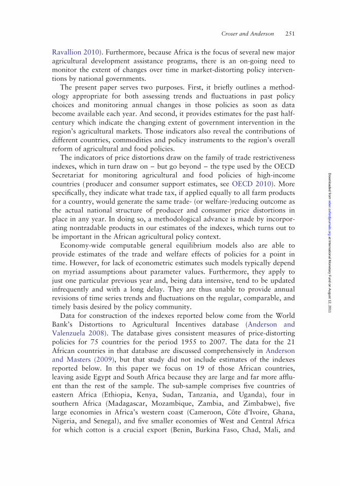
Ravallion 2010). Furthermore, because Africa is the focus of several new majoragricultural development assistance programs, there is an on-going need tomonitor the extent of changes over time in market-distorting policy interven-tions by national governments.

The present paper serves two purposes. First, it briefly outlines a method-ology appropriate for both assessing trends and fluctuations in past policychoices and monitoring annual changes in those policies as soon as databecome available each year. And second, it provides estimates for the past half-century which indicate the changing extent of government intervention in theregion’s agricultural markets. Those indicators also reveal the contributions ofdifferent countries, commodities and policy instruments to the region’s overallreform of agricultural and food policies.

The indicators of price distortions draw on the family of trade restrictivenessindexes, which in turn draw on – but go beyond – the type used by the OECDSecretariat for monitoring agricultural and food policies of high-incomecountries (producer and consumer support estimates, see OECD 2010). Morespecifically, they indicate what trade tax, if applied equally to all farm productsfor a country, would generate the same trade- (or welfare-)reducing outcome asthe actual national structure of producer and consumer price distortions inplace in any year. In doing so, a methodological advance is made by incorpor-ating nontradable products in our estimates of the indexes, which turns out tobe important in the African agricultural policy context.

Economy-wide computable general equilibrium models also are able toprovide estimates of the trade and welfare effects of policies for a point intime. However, for lack of econometric estimates such models typically dependon myriad assumptions about parameter values. Furthermore, they apply tojust one particular previous year and, being data intensive, tend to be updatedinfrequently and with a long delay. They are thus unable to provide annualrevisions of time series trends and fluctuations on the regular, comparable, andtimely basis desired by the policy community.

Data for construction of the indexes reported below come from the WorldBank’s Distortions to Agricultural Incentives database (Anderson andValenzuela 2008). The database gives consistent measures of price-distortingpolicies for 75 countries for the period 1955 to 2007. The data for the 21African countries in that database are discussed comprehensively in Andersonand Masters (2009), but that study did not include estimates of the indexesreported below. In this paper we focus on 19 of those African countries,leaving aside Egypt and South Africa because they are large and far more afflu-ent than the rest of the sample. The sub-sample comprises five countries ofeastern Africa (Ethiopia, Kenya, Sudan, Tanzania, and Uganda), four insouthern Africa (Madagascar, Mozambique, Zambia, and Zimbabwe), fivelarge economies in Africa’s western coast (Cameroon, Cote d’Ivoire, Ghana,Nigeria, and Senegal), and five smaller economies of West and Central Africafor which cotton is a crucial export (Benin, Burkina Faso, Chad, Mali, and

Croser and Anderson 251




Dow

nloaded from

Togo). We concentrate on 1961 to 2004, since those are the years for whichthe African data are most complete.

The paper is structured as follows: the next section summarizes the method-ology to be used. This is followed by a discussion of the data in the WorldBank’s Agricultural Distortions database. We then report estimates of the seriesof indexes, before drawing conclusions.

I . M E T H O D O L O G Y

There is a growing literature that identifies ways to estimate indicators of thetrade- and welfare-reducing effects of international trade-related policies asscalar index numbers. This literature serves a key purpose: it overcomes aggre-gation problems (across different intervention measures and across industries)by using a theoretically sound aggregation procedure to answer precise ques-tions regarding the trade or welfare reductions imposed by each country’s tradeand trade-related policies.

These measures represent a substantial improvement on commonly usedmeasures. The usual tools for summarizing price-distorting policy trends in acountry or region (see, e.g., Anderson and Masters 2009) are measures of theunweighted or weighted mean nominal rate of assistance (NRA) and consumertax equivalent (CTE), the standard deviation of industry NRAs for the sector,and in a few instances the weighted mean NRA for exportable versus import-competing covered products.1 Authors often need to report more than onemeasure to gain an appreciation of the nature of the policy regime. Forexample, indicators of dispersion of NRAs are a reminder that there areadditional welfare losses from greater variation of NRAs across industrieswithin the sector (Lloyd 1974). Further, if import-competing and exportablesub-sectors have NRAs of opposite sign, they need to be reported separatelybecause they would offset each other in calculating the aggregate sectoral NRA.

While those various indicators are useful as a set, policy makers would findit more helpful to have a single indicator to capture the overall trade or welfareeffect of an individual country’s regime of agricultural price distortions inplace at any time, and to trace its path over time and make cross-country com-parisons. To that end, the scalar index literature has been developed. The pio-neering theoretical work is by Anderson and Neary (summarized in their 2005book), with an important partial equilibrium contribution by Feenstra (1995).The theory defines an ad valorem trade tax rate which, if applied uniformlyacross all tradable agricultural commodities in a country will generate the same

1. The OECD (2010) measures similar indicators to the NRA and CTE, called producer and

consumer support estimates (PSEs and CSEs). The main difference from an African viewpoint, apart

from the CSE having the opposite sign to the CTE, is that the NRA and CTE are expressed as a

percentage divergence from undistorted (e.g., border) prices whereas the PSEs/CSEs relate to the

divergence from actual (distorted) prices.





Dow

nloaded from

reduction in sectoral trade, or in economic welfare, as the actual cross-productstructure of distortions.2

In recent years, several empirical papers have provided series of estimates ofscalar index numbers for individual countries. Irwin (2010) uses detailedimport tariff data to calculate the Anderson-Neary Trade Restrictiveness Indexfor the United States in 1859 and annually from 1867 to 1961; Kee, Nicitaand Olarreaga (2009) estimate indexes for 78 developing and developedcountries for a single point in time (the mid-2000s); and Lloyd, Croser andAnderson (2010) estimate indexes for 75 developed and developing countriesusing the World Bank’s Distortions to Agricultural Incentives database for theperiod 1955 to 2007.

In addition to being useful in summarizing the agricultural and food policyregime in an individual country, the Anderson-Neary scalar index measurescan be adapted to reveal two other aspects of agricultural policy: the relativecontributions of different policy instruments to reductions in trade or welfare(Croser and Anderson 2011), and the trade- and welfare-reducing effects ofpolicy in a single global or regional commodity market (Croser, Lloyd andAnderson 2010). In this paper we utilise the methodology to estimate all threetypes of indexes. In doing so, we extend the theory and analysis to include non-tradables, which have not been addressed in previous studies but which are ofpractical significance in poorer African countries where nontradables accountfor a non-trivial share of the gross value of agricultural production.

Country level trade- and welfare-reduction indexes

To capture distortions imposed by each country’s border and domestic policieson its trade volume and economic welfare, we adopt the methodology fromLloyd, Croser and Anderson (2010). Those authors define a Trade ReductionIndex (TRI) and a Welfare Reduction Index (WRI) and estimate them by con-sidering separately the distortions to the producer and consumer sides of theagricultural sector (which can differ when there are domestic measures in placein addition to or instead of trade measures). As their names suggest, the twoindexes respectively provide a single indicator the (partial equilibrium) of thetrade- or welfare-reducing effects of all distortions to consumer and producerprices of farm products from all agricultural and food policy measures in place.The TRI and WRI thus go somewhat closer to what a computable general equi-librium (CGE) can provide in the way of estimates of the trade and welfare(and other) effects of price distortions, while having the advantage of providingan annual time series. Fortuitously, estimates of the actual price distortions are

2. Other indexes define an ad valorem trade tax rate which, if applied uniformly across all tradable

products, will generate the same government revenue (Bach and Martin 2001), or the same real national

income and general equilibrium structure of the economy (Anderson 2009a), as the actual cross-product

structure of distortions.





Dow

nloaded from

available in the NRAs and CTEs of the World Bank’s Distortions toAgricultural Incentives database.

The derivation of the two indexes for n import-competing industries leads tothe expressions for the TRI and WRI for the import-competing sector of acountry shown in Box 1.

BOX 1: Expressions for the TRI and WRI

TRI WRI

T ¼ {RaþSb}, with

R ¼Pni¼1

riui

� �and S ¼

Pni¼1

sivi

� � W ¼ fR02aþ S02bg1=2, with

R0 ¼Pni¼1

r2i ui

� �12

and S0 ¼Pni¼1

s2i vi

� �12

where ui ¼ p�2i ðdxi=dpCi Þ=

Pi

p�2i ðdxi=dpCi Þ ¼ rið p�i xiÞ=

Pi

rið p�i xiÞ

vi ¼ p�2i ðdyi=dpPi Þ=P

i

p�2i ðdyi=dpPi Þ ¼ sið p�i yiÞ=

Pi

sið p�i yiÞ,

a ¼P

i

p�2i dxi=d pCi =P

i

p�2i dmi=dpi, and b ¼ �P

i

p�2i dyi=d pPi =P

i

p�2i dmi=dpi.

Variable definitions:

T — Trade Reduction Index; W — Welfare Reduction Index; R — index of average consumerprice distortions; S —index of average producer price distortions; R0 — Consumer DistortionIndex; S0 — Producer Distortion Index; si — the rate of distortion of the producer price in pro-portional terms; ri — rate of distortion of the consumer price in proportional terms; ui —weight for each commodity in R and R0, which is proportional to the marginal response ofdomestic consumption to changes in international free-trade prices and can be written as afunction of the domestic price elasticity (at the protected trade situation) of demand (ri); vi —weight for each commodity in S and S’, which is proportional to the marginal response ofdomestic production to changes in international free-trade prices and can be written as a func-tion of the domestic price elasticity (at the protected trade situation) of supply, (si); p�i —border price; pP

i ¼ p�i ð1þ siÞ— distorted domestic price; pCi ¼ p�i ð1þ riÞ — distorted domestic

consumer price; xi ¼ xiðpCi Þ — quantity of good i demanded (as a function of own domestic

price); yi ¼ yið pPi Þ — quantity of good i supplied (as a function of own domestic price); a (b)

— weight of consumption (production) in the WRI or TRI, which is proportional to the ratioof the marginal response of domestic demand (supply) to a price change relative to the mar-ginal response of imports to a price change.

Source: Synthesized from Lloyd, Croser and Anderson (2010)

Essentially the import-competing TRI and WRI are constructed from appropri-ately weighted averages of the level of distortions of consumer and producerprices. The TRI is a mean of order one, and the WRI a mean of order two, butthey use the same weights. Because the WRI is a mean of order two, it betterreflects the welfare cost of agricultural price-distorting policies because it recog-nizes that the welfare cost of a government-imposed price distortion is relatedto the square of the price wedge. It thus captures the disproportionately higherwelfare costs of peak levels of assistance or taxation, and is positive regardlessof whether the government’s agricultural policy is favouring or hurtingfarmers.





Dow

nloaded from

The TRI and WRI can each be extended so as to add the exportable andnontradable sub-sectors of agriculture (see Appendix). Distortions to exporta-ble industries are inputted into the TRI as negative values because a positive(negative) price distortion in an exporting industry has a trade-expanding (-reducing) effect, and thus decreases (increases) the TRI. Distortions to nontrad-able industries are inputted into the TRI as zero values because a domesticprice distortion in a nontradable industry by definition has neither atrade-expanding nor trade-reducing effect for that industry because of itsassumed prohibitively high trade costs.3

The expressions for the TRI and WRI weights above show that estimates ofown-price elasticities are required to compute the indexes. In line with Lloyd,Croser and Anderson (2010), and in the absence of reliable elasticity estimatesfor all countries and periods, we adopt some simplifying assumptions in thispaper. We assume that a country’s domestic price elasticities of supply areequal across commodities within a sub-sector, and likewise for domestic priceelasticities of demand. This powerful simplifying assumption allows us (in theempirical section below) to find appropriately weighted aggregates of distor-tions on the production and consumption sides of the market simply by aggre-gating the change in consumer (producer) prices across commodities and usingas weights the sectoral share of each commodity’s domestic value of consump-tion (production) at undistorted prices.

We expect these simplifying elasticity assumptions (which still allow fordifferences across countries and between the demand and supply elasticities ofeach product within each country) to have only a small impact on the reportedindexes. This is because elasticities appear in both the numerator and denomi-nator of the weight expressions, and therefore cancel each other out to a con-siderable extent. Further, Kee, Nicita and Olarreaga (2008, p. 677) show thatthe TRI and WRI can be decomposed into three components (namely, themean and the variance of the distortion rates and the co-variance between thesquare of the distortion rate and the appropriate price elasticity). Since the elas-ticity enters into only the third component (see Appendix), and since in prac-tice that component tends to be small relative to the other two components (asnoted by Anderson and Neary (2005) and found empirically by Kee, Nicitaand Olarreaga (2009) and Irwin (2010)), errors from adopting these simplify-ing elasticity assumptions are unlikely to be a major problem. These assump-tions also make practical sense in the context of computing time series ofindexes for Africa, where there is a dearth of reliable and consistent estimatesof price elasticities of demand and supply for different time periods over the

3. It is conceivable that a distortion to the price of a nontradable could have an indirect trade

consequence because of non-zero cross-price elasticities of demand or supply between tradables and

nontradables. However, as with estimates of NRAs and CTEs, our estimates of TRIs and WRIs assume

those cross-price elasticities (and also those between tradable products) are zero. We make this

assumption not only to simplify greatly the algebra but also because reliable estimates of all the relevant

cross elasticities for Africa over the 45-year period under review are unavailable.





Dow

nloaded from

past half-century for each of the covered agricultural products in each of ourfocus countries.4

Policy instrument trade and welfare reduction indexes

The above country-level TRI and WRI measures are the aggregate of the trade-or welfare-reducing indicators of all the policy measures in place. The variablessi and ri, as domestic-to-border price ratios, can theoretically encompass distor-tions provided by all trade tax/subsidy and non-tariff trade measures, plusdomestic price support measures (positive or negative), plus direct interven-tions affecting farm input prices. Furthermore, where multiple exchange ratesoperate, the measures can encompass an estimate of the import or export taxequivalent of that distortionary regime too.

Whilst it is desirable to have such an aggregated country level indicator thatis so encompassing, agricultural policy analysts are sometimes interested also inindicators of the relative contribution of different policy instruments toreductions in trade or welfare. To provide this insight, it is possible to use theAnderson-Neary framework to construct indexes of policy distortions at theinstrument level to facilitate this comparison.5

To capture distortions imposed by each African country’s different policyinstruments on its trade volume and its economic welfare, we adopt the meth-odology from Croser and Anderson (2011). These authors define anInstrument Trade Reduction Index (ITRI) and an Instrument WelfareReduction Index (IWRI), which can be estimated by considering the distortionfrom a single policy instrument to the producer and consumer sides of themarket.

The methodology in Croser and Anderson (2011) identifies four types ofborder distortions (import taxes and subsidies, and export taxes and subsidies),for which individual ITRI and IWRI series can be estimated. In addition to theborder measures, the series for domestic distortions in the form of production,consumption and input taxes and subsidies can be estimated. To estimate thetrade-reducing effect of an individual instrument, those authors deriveexpressions for the change in import volume from the individual policymeasures, which are used as the basis for deriving ITRIs. To estimate thewelfare-reducing effect of individual instruments, those authors make anassumption about the allocation of the total welfare loss from the combinationof individual policy instruments. They assume that border measures are appliedfirst, and that this may be supplemented by additional domestic price

4. Sensitivity analysis by Croser, Lloyd and Anderson (2010) shows little difference in the overall

TRI and WRI estimates for commodities globally when differentiated elasticity estimates from Tyers

and Anderson (1992) were used in place of common ones in each country.

5. Note that most of the series of TRI and WRI indicators in the literature are for single instruments

anyway. For example, Irwin (2010) uses only import tariffs, and Kee, Nicita and Olarreaga (2009)

report two series of indexes — one based on tariffs only, the other on tariffs plus non-tariff import

barriers.





Dow

nloaded from

distortions (which, in practice for Africa, are relatively minor). Thus the dom-estic distortion’s welfare reduction is the residual from subtracting the bordermeasures’ effects from the total welfare reduction of all policy measures. Thisallocation assumption provides a lower-bound on welfare losses from bordermeasures and an upper-bound on welfare losses from domestic measures.

The derivation of the ITRI and IWRI follows essentially the same steps asthose for the country-level indexes which encompass all forms of price distor-tion. The difference in the algebraic methodology is to specify separate indexesfor the nine different types of policy instrument (for details see Croser andAnderson 2011). Simplifying assumptions can be made in the absence ofreliable price elasticity estimates, and again these assumptions have a minimaleffect on the estimates.

Commodity market trade and welfare reduction indexes

In addition to constructing country-level and instrument-specific indexes, thispaper makes use of another methodology within the Anderson-Neary frame-work to analyse a different aspect of agricultural policy in Sub-Saharan Africa.We construct indexes that show the extent to which African markets for indi-vidual farm commodities are distorted relative to others. We employ the meth-odology in Croser, Lloyd and Anderson (2010) for this purpose. Thismethodology is novel because whereas all previous work within the traderestrictiveness indexes literature has focused on constructing index numbers ofdistortions from the perspective of a single country, this methodology insteadtakes a regional view of individual commodity markets.

The regional commodity TRI (WRI) is equal to the uniform trade tax thathas the same effect on regional trade volume (welfare) as the existing set of dis-tortions in the region’s national commodity markets. The measures are con-structed in the same way as those for individual country indexes, except thatinstead of summing across distortions in different industries for a singlecountry, the measures are constructed by summing across distortions in differ-ent countries for a single commodity. The indexes are computed using data onthe domestic production and consumption sides of the region’s national com-modity markets, and the measures account for all forms of border and dom-estic price distortions in each country for the commodity market of interest, aswell as incorporating import-competing and exportable countries into themeasure.

I I . D I S T O R T I O N S T O A G R I C U L T U R A L I N C E N T I V E S D A T A B A S E

This study makes use of the World Bank’s Distortions to AgriculturalIncentives database (Anderson and Valenzuela 2008). The database is anoutput from a global research project seeking to improve the understanding ofagricultural policy interventions and reforms in Asia, Europe’s transition econ-omies, Latin America and the Caribbean as well as Africa. The database





Dow

nloaded from

contains annual estimates of nominal rates of assistance (NRA) (positive ornegative) for key farm products in 75 countries that together account forbetween 90 and 96 percent of the world’s population, farmers, agriculturalGDP, and total GDP. There are 21 African countries in the database.

We concentrate on the sample of 19 Sub-Saharan African countries listed inthe introduction, excluding relatively affluent Egypt and South Africa. Forthose 19 African focus countries, the database contains around 6000 consistentestimates of annual NRAs to the agricultural sector between 1955 and 2004 or2005, and the same number of CTEs. Country coverage up to 1960 is muchless than from 1961, so the series of estimates presented in this paper begins inthat latter year.

The estimates of NRA and CTE in the database are at the commodity leveland cover a subset of 41 agricultural products in Africa. These so-calledcovered products account for around 70 percent of each country’s total agricul-tural production over the period studied. The data identifies each year whethereach commodity in each country is considered an importable, exportable ornontradable, a status that may change over time. In the 19 African focuscountries, tradable products account for between 40 and 55 percent of thegross value of production of all covered agricultural products (last column ofTable 1).

The range of policy measures included in the NRA estimates in theDistortions to Agricultural Incentives database is wide. By calculatingdomestic-to-border price ratios, the estimates include assistance provided by alltariff and nontariff trade measures, plus any domestic price support measures(positive or negative), plus an adjustment for the output-price equivalent ofdirect interventions affecting prices of farm inputs. Where multiple exchangerates operate, estimates of the import or export tax equivalents of that distor-tion are included as well. The range of measures included in the CTE estimatesinclude both domestic consumer taxes and subsidies and trade and exchangerate policies, all of which drive a wedge between the price that consumers payfor each commodity and the international price at the border.

Anderson and Masters (2009) note several patterns that emerge in the distor-tions to agricultural incentives in the focus countries. In the 1960s and 1970s,many African governments had macroeconomic, sectoral and trade policiesthat increasingly favored the urban sector at the expense of farm households,and favored production of import-competing farm goods at the expense ofexportables. The policy regime was characterized as pro-urban (anti-agricultural) and pro-self-sufficiency (anti-agricultural trade). Since the 1980s,Africa has reduced its anti-agricultural and anti-trade biases, but many distor-tions still remain.

For the countries in this study, Table 1 and Figure 1 illustrate those patterns.The weighted average NRA for the 19 countries is almost always below zero,indicating that agricultural price, trade and exchange rate policies togetherhave reduced the earnings of farmers in these countries. The average rate of





Dow

nloaded from

TA B L E 1. Nominal Rates of Assistance for import-competing, exportable andnontradable covered agricultural products, 19 African focus countries,a 1961to 2004

(percent)

NRA, agricultural productsa Tradablesshare (%)of value ofall coveredagriculturalproduction

Coveredexportables

Coveredimportables

Allcovered

tradablesbCovered

nontradables

Allcoveredproducts

Standarddeviationof NRAsb

1961–64 230 123 3 0 21 34 491965–69 239 62 215 0 211 33 551970–74 247 30 227 0 217 31 551975–79 252 22 230 21 223 37 541980–84 247 4 228 21 218 35 461985–89 250 49 226 22 215 33 461990–94 249 5 227 22 216 31 411995–99 232 3 215 23 210 25 392000–04 232 7 216 23 210 26 43

Source: Anderson and Valenzuela (2008)

a. Nominal rates of assistance for the 19 African focus countries are weighted by the grossvalue of production at undistorted prices for the relevant sub-sector.

b. The simple average of the 19 focus countries’ standard deviation of NRA around itsweighted mean.

FIGURE 1. Nominal Rates of Assistance for import-competing, exportable andall covered agricultural products, 19 African countries, 1961 to 2004

Source: Anderson and Valenzuela (2008).





Dow

nloaded from

direct taxation (negative NRA) of African farmers rose until the late 1970sbefore declining by more than half over the next 25 years.

Table 2 reports the country-level NRAs for covered products for each of the19 countries in this sample. It reveals the considerable diversity within thesample. In some countries — such as Cameroon, Ghana, Senegal, Uganda,Tanzania, and Madagascar —a reduction in the taxing of farmers is evidentfollowing the regional peak in 1975–79, while in other countries — such asCote d’Ivoire, Zambia, and Zimbabwe — high levels of agricultural taxationappear to have persisted.

The country level aggregate measures hide the degree of variation in NRAestimates within countries. Column 6 of Table 1 suggests the standard devi-ations around the weighted mean NRA for covered products in each countryhas been high, but has declined somewhat since the mid-1990s. An indicationof the extent of variation between groups of products is seen even when com-paring the average NRAs for import-competing and exportable product groups(Figure 1). The gap between those two groups’ average NRAs has tended tonarrow over the period shown, suggesting there has been a decline also in theanti-trade bias in Africa’s agricultural policies since the mid-1990s.

TA B L E 2. Nominal rates of assistance, all covered agricultural products, 19African focus countries, 1961 to 2004

(percent)

1961–64

1965–69

1970–74

1975–79

1980–84

1985–89

1990–94

1995–99

2000–04

Africa -1 -11 -17 -23 -18 -15 -16 -10 -10

Benin na na 23 21 21 21 24 24 21Burkina Faso na na 22 23 24 21 23 23 0Cameroon 24 28 212 225 219 25 24 24 21Chad na na 212 211 28 21 23 23 21Cote d’Ivoire 229 235 233 240 240 228 222 222 228Ethiopia na na na na 212 215 217 210 27Ghana 215 228 223 241 232 28 23 25 22Kenya 13 22 224 215 230 28 230 24 4Madagascar 219 223 220 238 251 226 27 24 2Mali na na 26 28 27 23 25 27 0Mozambique na na na 256 242 251 24 5 14Nigeria 21 12 7 5 8 15 4 0 25Senegal 215 212 233 234 230 5 7 210 212Sudan 226 237 248 228 233 239 254 229 215Tanzania na na na 250 260 252 230 229 217Togo na na 21 21 22 22 24 23 21Uganda 23 25 212 224 212 214 21 1 1Zambia 224 232 242 257 226 268 253 234 236Zimbabwe 236 236 244 254 247 243 245 238 273

Source: Anderson and Valenzuela (2008)





Dow

nloaded from

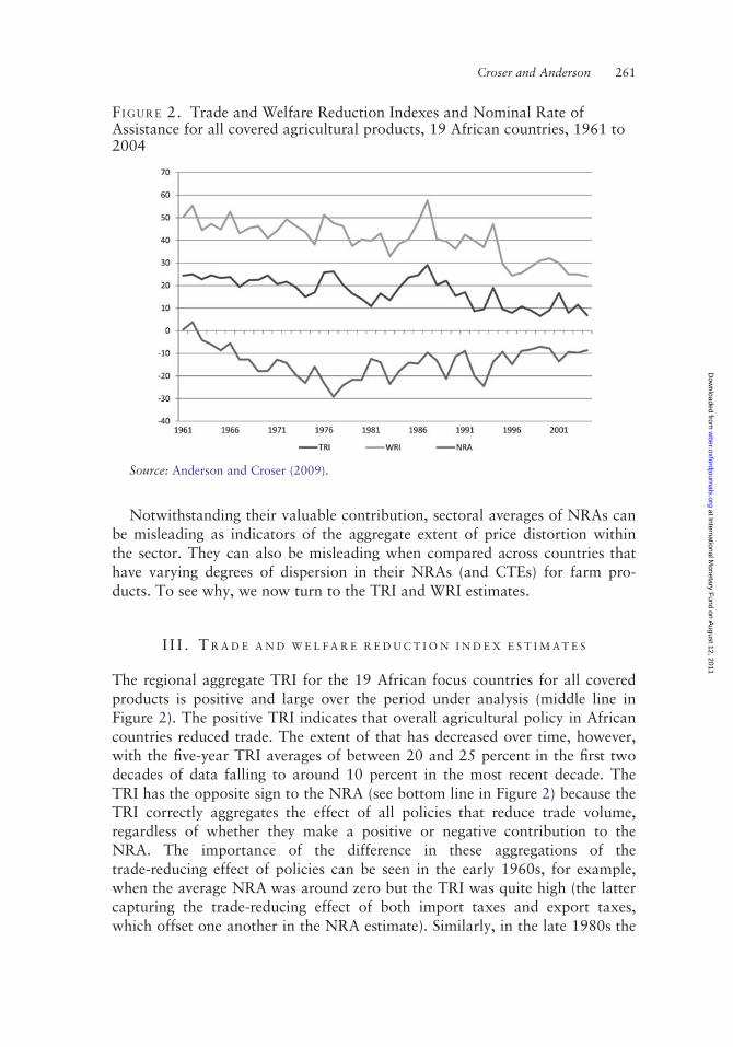
Notwithstanding their valuable contribution, sectoral averages of NRAs canbe misleading as indicators of the aggregate extent of price distortion withinthe sector. They can also be misleading when compared across countries thathave varying degrees of dispersion in their NRAs (and CTEs) for farm pro-ducts. To see why, we now turn to the TRI and WRI estimates.

I I I . T R A D E A N D W E L F A R E R E D U C T I O N I N D E X E S T I M A T E S

The regional aggregate TRI for the 19 African focus countries for all coveredproducts is positive and large over the period under analysis (middle line inFigure 2). The positive TRI indicates that overall agricultural policy in Africancountries reduced trade. The extent of that has decreased over time, however,with the five-year TRI averages of between 20 and 25 percent in the first twodecades of data falling to around 10 percent in the most recent decade. TheTRI has the opposite sign to the NRA (see bottom line in Figure 2) because theTRI correctly aggregates the effect of all policies that reduce trade volume,regardless of whether they make a positive or negative contribution to theNRA. The importance of the difference in these aggregations of thetrade-reducing effect of policies can be seen in the early 1960s, for example,when the average NRA was around zero but the TRI was quite high (the lattercapturing the trade-reducing effect of both import taxes and export taxes,which offset one another in the NRA estimate). Similarly, in the late 1980s the

FIGURE 2. Trade and Welfare Reduction Indexes and Nominal Rate ofAssistance for all covered agricultural products, 19 African countries, 1961 to2004

Source: Anderson and Croser (2009).





Dow

nloaded from

NRA changes from around 215 percent to 210 percent at a time when theTRI increases from 20 to 30 percent: the aggregate NRA gives the impressionthat policies are becoming less distorted in this period but, because the upwardtrend in the NRA is caused by an increase in import taxes, the TRI correctlyreveals that agricultural policies are in fact becoming more trade-restrictive inthis time period.

The WRI series for all covered products is necessarily positive and every-where lies above the TRI series (compare middle and upper lines in Figure 2).The WRI series correctly demonstrates the negative welfare consequences thatflow from both negative and positive price distortions. Furthermore, the WRIseries provides a better indicator of the welfare cost of distortions than theaverage level of assistance or taxation, due to the inclusion in the WRI of the‘power of two’. A weighted arithmetic mean does not fully reflect the welfareeffects of agricultural distortions because the dispersion of that support ortaxation across products has been ignored. By contrast, the WRI captures thehigher welfare costs of peak levels of assistance or taxation.

The aggregate African results mask country-level diversity in the TRI andWRI series. Some countries — such as Cote d’Ivoire, Ethiopia, Sudan,Tanzania and Zimbabwe — persistently restricted trade (in aggregate) through-out the period under analysis (Table 3). Other countries — such as Kenya,Mozambique and Zambia — have had periods in which policies in aggregatehave expanded agricultural trade slightly (via import subsidies). In terms of theWRI, there is less diversity across countries, since WRI measures are all necess-arily positive (Table 4). The extent to which agricultural policy reduced aggre-gate welfare does differ across countries, however. Some countries have lowreductions in welfare, including Uganda and most cotton-exporting countries.Figure 3 provides a snapshot for 2000–04 of the diversity in the WRI and TRIfor each of the 19 countries, with the weighted African average in the middleand close to Kenya.

A useful way of understanding the overall welfare reduction for Africa fromagricultural policy is to compute the country contributions to the WRI for the19 African focus countries as a whole. Contributions can be found by comput-ing dollar values of the welfare reduction index for each country (by multiply-ing the WRI percent by the average of the gross value of production andconsumption at undistorted prices). Table 5 shows that Nigeria, Sudan andEthiopia dominate the region’s contributions. The last column of Table 5reports country contributions to the decline in the regional WRI from its valueof 44 percent in 1975–79 to its value of 27 percent in 2000–04. Nigeria andSudan dominate that overall reduction, together accounting for around 80percent of the fall in the WRI. However, Cameroon, Madagascar, Senegal andUganda have slightly offsetting effects on the regional fall in the WRI over thatperiod.

It is worth noting that the TRI and WRI for all covered products is signifi-cantly lower than that for just tradables. This is because nontradables account





Dow

nloaded from

for a large share of the gross value of production and consumption (see finalcolumn of Table 1). The TRI estimates for all covered products are roughlyhalf, and WRI estimates are roughly two-thirds, what there are with nontrad-ables excluded.

It is useful to compare the TRI and WRI results for the African focuscountries with those for other developing country regions, which are reportedin Lloyd, Croser and Anderson (2010). The African focus countries’ policieshave been, and remain, the most trade- and welfare-reducing. However, allthree regions have shown a trend towards less damaging agricultural policies inrecent years (Figure 4).

Policy instrument results

We now turn to the national decompositions of the TRI and WRI to the policyinstrument level. Figure 5 provides a summary of the estimates of the contri-bution to the weighted average WRI series for the 19 African focus countriesof four different border measures: taxes and subsidies on both imports and

TA B L E 3. Trade Reduction Index, all covered agricultural productsa, 19African focus countries, 1961 to 2004

(percent)

1961–64

1965–69

1970–74

1975–79

1980–84

1985–89

1990–94

1995–99

2000–04

Africa 24 22 20 21 15 24 14 9 10


Source: Anderson and Croser (2009) based on NRA and CTE data in Anderson andValenzuela (2008).

a. Includes all import-competing, exportable and nontradable products, with nontradablesectors assumed to have a zero level of distortion on the volume of trade.





Dow

nloaded from

exports. The figure demonstrates the very substantial role that export taxeshave played in the reduction of welfare in the region. On average, more thanhalf the welfare reductions has come from anti-agricultural export taxing pol-icies over the period studied, but the decline in them has contributed most toreform in recent decades: the gross contribution of export taxes to thereduction in the WRI over the period 1985–89 to 2000–04 is 93 percent. Theremaining 7 percent is made up of a 34 percent gross contribution from importtax cuts offset by a 228 percent contribution from export subsidies(213 percent) and import subsidies (215 percent).

The contributions to TRI and WRI estimates for African countries fromdomestic distortions are small, never accounting for more than 5 percent of theoverall regional TRI or WRI. This can be seen in Table 6. That table alsoreveals the far greater dominance of export taxation in Africa as comparedwith developing Asia and Latin America, particularly in the 2000-04 period.

Commodity TRI and WRI results

The TRI and WRI estimates for individual regional commodity marketsprovide a different perspective on the level of distortion in the focus countries

TA B L E 4. Welfare Reduction Index, all covered agricultural products, 19African focus countries, 1961 to 2004

(percent)

1961–64

1965–69

1970–74

1975–79

1980–84

1985–89

1990–94

1995–99

2000–04

Africa 49 46 45 44 39 45 40 28 27


Source: Anderson and Croser (2009) based on NRA and CTE data in Anderson andValenzuela (2008).





Dow

nloaded from

over the period under analysis. Table 7 reveals considerable diversity in the dis-tortions in different commodity markets in Africa. Fruit and vegetable com-modity markets, which tend to have a high share of nontradable production,have low WRI estimates on average, whereas traded commodities such as tropi-cal crops, oilseeds and livestock tend to have more welfare-reducing policies inplace. Grains, which comprise a mixture of tradable and nontradable products,had highly-distortionary policies in the 1960s on average, but these have beenreduced over time. As of 2000–04, the indexes suggest sugar and cottonmarkets continue to have highly distorted policies in terms of both the tradeand welfare effects of their policies.

I V. C O N C L U S I O N S

Reform of agricultural policy in Africa is topical at present. Recentlyannounced international aid and investment programs, domestic policyreforms, and the negotiation of international and regional trade agreements areon the agenda, not to mention climate change. Measurement of interventionlevels is required to assess policy initiatives in each of these areas. Certainly

FIGURE 3. Trade and Welfare Reduction Indexes, all covered agriculturalproducts, 19 African countries and regional averagea, 2000-04

Source: Anderson and Croser (2009)a. To get the African regional average, the national indexes are weighted by the average of the

gross value of production and consumption at undistorted prices.





Dow

nloaded from

economy-wide models can measure the welfare and trade (and other) effects ofpolicy in a particular country or market, and do it better than can partial equi-librium analysis where there are potentially offsetting policies such as importtaxes and import subsidies. Such models require, however, reliable data on thestructure of the economy and sound econometric estimates of myriad par-ameters, neither of which are easily found for the poorer countries of Africa.Even where economy-wide models are available, they are calibrated to a par-ticular year (typically 5þ years ago) and are incapable of providing easilyupdatable time series indicators of the national and regional effects of distor-tional policies.

Scalar index measures, by contrast, can provide meaningful partial equili-brium indicators of the welfare and trade effects of policy interventions in agri-culture in poorer countries. As demonstrated above, these indexes can be

TA B L E 5. Country contributionsa to the regional Welfare Reduction Index forAfrican focus countries,b all covered agricultural products, 1961 to 2004, andto its fall from 1975-79 to 2000-04

(percent)

1961–64 1970–74 1980–84 1990–94 2000–04

Contributionto fall in

WRI between1975–79 and

2000–04Africa WRI 49 45 39 40 27

Cameroon 2 3 2 1 0 24Cote d’Ivoire 3 5 6 4 5 1Ethiopia - - 10 10 9 naGhana 2 3 4 2 3 1Kenya 2 2 3 3 2 1Madagascar 1 3 4 1 1 22Mozambique - - 2 1 2 2Nigeria 74 51 37 38 35 34Senegal 1 2 2 2 1 23Sudan 10 21 18 30 27 44Tanzania - - 7 3 6 1Uganda 1 4 4 0 1 28Zambia 1 2 1 1 2 1Zimbabwe 3 4 3 3 5 7Africa 100 100 103 100 100 100

Source: Authors’ calculations from data in Anderson and Croser (2009).

a. Country contributions are computed by converting national percentage WRIs to dollarvalues by multiplying by the average of the gross value of production and consumption at undis-torted prices.

b. Benin, Burkina Faso, Chad, Mali, and Togo are not shown as each of their contributionswas less than 0.5 percent.





Dow

nloaded from

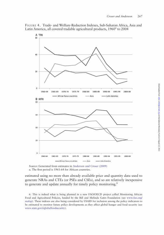
estimated using no more than already available price and quantity data used togenerate NRAs and CTEs (or PSEs and CSEs), and so are relatively inexpensiveto generate and update annually for timely policy monitoring.6

FIGURE 4. Trade- and Welfare-Reduction Indexes, Sub-Saharan Africa, Asia andLatin America, all covered tradable agricultural products, 1960a to 2004

Source: Generated from estimates in Anderson and Croser (2009)a. The first period is 1961-64 for African countries.

6. This is indeed what is being planned in a new FAO/OECD project called Monitoring African

Food and Agricultural Policies, funded by the Bill and Melinda Gates Foundation (see www.fao.org/

mafap). These indexes are also being considered by USAID for inclusion among the policy indicators to

be estimated to monitor future policy developments as they affect global hunger and food security (see

www.state.gov/s/globalfoodsecurity).





Dow

nloaded from

The scalar index numbers reported in this paper are thus a major sup-plement to the widely-used price distortion measures such as NRAs or PSEs,because they correctly aggregate offsetting policies and because the WRI prop-erly captures the much higher welfare costs associated with the largest pricedistortions. True, the indexes measured in this study (like NRAs or PSEs) donot make use of price elasticity estimates, but if and when reliable estimatesbecome available for the many agricultural products of the region, they can beincorporated to revise our estimates. Meanwhile, both theory and other recentempirical studies (see, e.g, Croser, Lloyd and Anderson 2010) provide comfortin suggesting the use of differentiated elasticity estimates across commoditieswould not make much difference to the results.

The methodology in the paper adopts the standard partial equilibriumapproach still presented in most textbooks on trade policy or welfare econ-omics. In particular, it is based on the benchmark of competitive markets. Themethodology ignores the existence of divergences such as externalities and gov-ernance problems, including administrative costs. The trade and welfarereduction indexes reported above may be over- or under-stated to the extentthat such problems exist. For example, in some cases where there is marketfailure, we know from second-best theory that policies that increase assistanceto a lightly protected sector may increase rather than decrease national econ-omic welfare. Even so, the series reported in this paper almost certainly give abetter indication of trade and welfare effects of policies than the NRA/CTEmeasures from which they are built.

FIGURE 5. Decomposition of the Welfare Reduction Index due to bordermeasures, by policy instrument, 19 focus African countries, 1961 to 2004

Source: Croser and Anderson (2011).





Dow

nloaded from

Notwithstanding those caveats, two clear conclusions can be drawn from theempirical estimates presented in this paper. One is that they confirm that there hasbeen very substantial policy reform in African agriculture over recent decades,especially in phasing out export taxation. The other is that they reveal there is stilla long way to go before that reform process is complete, since the trade- and

TA B L E 6. Contributions from different policy instruments on the productionside to the TRI and WRI for covered products by different policy instruments,a

by developing country region,b 1980–84 and 2000–04

(percent)

(a) TRI

1980-84 2000-04

Africa Asia Latin Amer. Africa Asia Latin Amer.

All measures 24 37 21 16 10 7

Border measures 22 33 20 13 9 7

Export tax 24 27 21 15 2 6Export subsidy 24 21 21 23 21 23Import tax 10 9 6 7 10 5Import subsidy 28 22 25 26 21 22

Domestic taxes & subsidies 2 4 1 3 1 0

Production tax 2 3 0 3 1 0Production subsidy 0 0 1 0 0 0

(b)WRI

1980-84 2000-04

Africa Asia Latin Amer. Africa Asia Latin Amer.

All measures 54 61 46 38 20 25

Border measures 48 44 38 33 17 18

Export tax 25 29 23 16 2 7Export subsidy 4 1 1 3 3 3Import tax 11 12 7 8 12 7Import subsidy 8 2 6 6 1 2

Domestic taxes & subsidies 6 17 8 5 3 7

Production tax 5 15 1 4 1 2Production subsidy 1 1 8 0 2 5

Source: Croser and Anderson (2011).

a. Each instrument share is computed in the following two steps: (1) indices are converted toconstant 2000 $US by multiplying the index by the average value of production or consumptionfor that instrument group at the country level; (2) each instrument dollar amount index is dividedby the country average value of production or consumption. The measures in the table — whichare like a weighted average of an overall regional index — therefore reflect both the absolute sizeof the index for each policy instrument and the relative importance of that policy instrument inthe region.

b. Africa includes Egypt and South Africa (unlike in previous tables); Asia excludes Japan;Latin America includes the Caribbean.





Dow

nloaded from

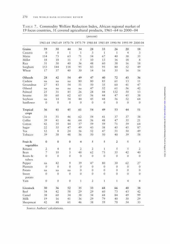
TA B L E 7. Commodity Welfare Reduction Index, African regional market of19 focus countries, 31 covered agricultural products, 1961–64 to 2000–04

(percent)

1961-64 1965-69 1970-74 1975-79 1980-84 1985-89 1990-94 1995-99 2000-04

Grains 59 50 44 34 28 33 26 20 18

Cassava 0 0 1 1 3 1 1 4 3Maize 114 73 63 71 54 67 40 38 35Millet 18 18 11 5 10 13 16 18 8Rice 31 30 40 36 48 60 38 16 18Sorghum 153 144 118 95 83 95 80 52 49Wheat 17 37 40 30 14 16 35 16 16

Oilseeds 28 42 54 49 47 40 72 43 36

Cashew na na na 80 80 85 61 13 11Groundnut 27 43 54 51 50 35 60 41 47Oilseed na na na na 47 52 61 56 42Palmoil 25 31 45 26 28 44 132 50 13Sesame 50 60 62 65 56 44 47 45 38Soybean na 14 34 44 45 44 56 52 64Sunflower 0 0 0 0 0 0 0 0 0

Tropical

crops

36 41 45 61 54 49 53 44 51

Cocoa 31 51 46 62 54 41 37 37 38Coffee 39 41 46 64 56 48 47 35 21Cotton 42 35 44 57 59 59 71 59 64Sugar 22 35 47 49 43 38 45 45 87Tea 12 8 24 56 52 47 51 50 49Tobacco 39 38 48 56 50 50 40 39 58

Fruit &

vegetables

0 0 0 4 5 5 2 5 5

Banana 2 4 0 2 2 1 5 5 2Bean 7 10 3 48 62 73 35 42 40Roots &

tubers0 0 0 0 0 0 0 0 0

Pepper na 42 9 39 47 80 30 62 27Plantain 0 0 0 0 0 0 0 0 0Potato na na na 0 0 0 0 0 0Sweet

potato0 0 0 0 0 0 0 0 0

Yam 0 0 0 1 2 1 1 4 4

Livestock 30 36 52 35 33 68 66 40 38

Beef 34 42 58 29 29 60 73 43 42Camel 38 60 34 38 34 68 84 49 99Milk 19 16 41 36 29 79 40 30 29Sheepmeat 42 48 61 46 38 59 70 54 33

Source: Authors’ calculations.





Dow

nloaded from

welfare-reduction indexes associated with the present decade’s policies are stillsubstantial and reveal large differences across countries and commodities.

F U N D I N G

This work is a product of a World Bank research project on Distortions toAgricultural Incentives (Project P093895, see www.worldbank.org/agdistortions) which was financially supported by the governments of theNetherlands (BNPP), the United Kingdom (DfID) and Ireland; and by theAustralian Research Council (DP0880565).

AC K N O W L E D G E M E N T S

The authors are grateful for helpful referee comments and for the distortionestimates provided by the authors of the various African country case studies,reported in Anderson, K. and W. Masters (eds.), Distortions to AgriculturalIncentives in Africa, Washington DC: World Bank, 2009. The views expressedare the authors’ alone and not necessarily those of the World Bank and itsExecutive Directors, nor the countries they represent, nor of the institutionsproviding the project research funds.

A P P E N D I X : D E R I VA T I O N O F T R A D E - A N D W E L F A R E - R E D U C T I O N

I N D E X E S

Lloyd, Croser and Anderson (2010) outline a methodology for computing indexeswhich accurately capture the state of trade policy regime in an individual countryin a theoretically meaningful way. Their methodology, which draws heavily onthe Anderson and Neary (2005) methodology, defines partial equilibrium indexeswhich aggregate the production and consumption sides of the economy separately(instead of trade data as is more commonly done with trade restrictivenessindexes). This form of index is well-suited to agricultural distortions research,where data are available for production and consumption of individual farm com-modities. This Appendix briefly outlines that theory for the import-competingsector of a small open economy (with further details and extensions available inLloyd, Croser and Anderson 2010 and Croser, Lloyd and Anderson 2010).

Consider an individual country and assume it has a small, open economy inwhich all markets are competitive. The market for an import good may be dis-torted by a tariff and other nontariff border measures or by behind-the-bordermeasures such as domestic subsidies and price controls. The effect of a coun-try’s distortions on its import volume is captured by the Trade ReductionIndex (TRI), defined as the uniform tariff rate which, if applied to all goods inthe place of all actual border and behind-the-border price distortions, wouldresult in the same reduction in the volume of imports (summed across productsby valuing them at the undistorted border price) as the actual distortions.





Dow

nloaded from

Suppose the market for one good, good i, is distorted by a combinationof measures that distort its consumer and producer prices. For the producersof the good, the distorted domestic producer price, pP

i , is related to theborder price, p�i , by the relation, pP

i ¼ p�i ð1þ siÞ where si is the rate of distor-tion of the producer price in proportional terms. For the consumers of thegood, the distorted domestic consumer price, pC

i , is related to the borderprice by the relation, pC

i ¼ p�i ð1þ riÞ where ri is the rate of distortion of theconsumer price in proportional terms. In general, ri = si . Using theserelations, the change in the value of imports in the market for good i isgiven by:

DMi ¼ p�i Dxi � p�i Dyi

¼ p�2i dxi=d pCi ri � p�2i dyi=d pP

i si

ð1Þ

where the quantities of good i demanded and supplied, xi and yi, arefunctions just of their own domestic price: xi ¼ xiðpC

i Þ and yi ¼ yiðpPi Þ.

Strictly speaking, this result holds only for small distortions. In reality ratesof distortion may not be small. If, however, the demand and supply functionsare linear over the relevant price range, the effect on imports is given byequation (1) with constant slopes of the demand and supply curves (dxi / dpC

i

and dyi / dpPi , respectively). If the functions are not linear, this expression pro-

vides an approximation to the loss.With n importable goods subject to different levels of distortions, the aggre-

gate reduction in imports, in the absence of cross-price effects in all markets, isgiven by:

DM ¼Xn

i¼1

p�2i dxi=d pCi ri �

Xn

i¼1

p�2i dyi=d pPi si ð2Þ

Setting the result equal to the reduction in imports from a uniform tariff,T, gives:

Xn

i¼1

p�2i dxi=d pCi ri �

Xn

i¼1

p�2i dyi=d pPi si ¼

Xn

i¼1

p�2i dmi=dpiT

Solving for T, gives

T ¼ fRaþ Sbg ð3aÞ

where R ¼Xn

i¼1

riui

" #with ui ¼ p�2i dxi=d pC

i =X

i

p�2i dxi=d pCi ; ð3bÞ

S ¼Xn

i¼1

sivi

" #with vi ¼ p�2i dyi=d pP

i =X

i

p�2i dyi=d pPi ; and ð3cÞ





Dow

nloaded from

a ¼X

i

p�2i dxi=d pCi =X

i

p�2i dmi=dpi; and

b ¼ �X

i

p�2i dyi=d pPi =X

i

p�2i dmi=dpi

ð3dÞ

Evidently, the uniform tariff T can be written as a weighted average of thelevel of distortions of consumer and producer prices, R and S (the Consumerand Producer Assistance Indexes, respectively). An important advantage ofusing this decomposition of the index into producer and consumer effects isthat it treats correctly the effects of non-tariff measures and domestic distor-tions that affect the two sides of the market differently.

In equation 3c (equation 3b), the weights for each commodity are pro-portional to the marginal response of domestic production (consumption) tochanges in international free-trade prices. These weights can be written as,among other things, functions of the domestic price elasticities (at the protectedtrade situation) of supply and demand (si and ri, respectively):7

ui ¼ rið p�i xiÞ=Xn

i

rið p�i xiÞ and vi ¼ sið p�i yiÞ=Xn

i

sið p�i yiÞ ð4Þ

The other index defined in Lloyd, Croser and Anderson (2010), the WelfareReduction Index (WRI), measures the effect of a country’s distortions on itseconomic welfare. The derivation follows the same steps as in the derivation ofthe TRI except that instead of starting from the loss in trade volume from apolicy, one starts from a loss of consumer and producer surplus (a welfare loss,Li). With n importable goods subject to different levels of distortions, theaggregate welfare loss, in the absence of cross-price effects in all markets, isgiven by:

L ¼1

2

Xn

i¼1

ð p�i siÞ2dyi=d pPi �

Xn

i¼1

ð p�i riÞ2dxi=d pCi

( )ð5Þ

The uniform tariff rate, W, that generates an aggregate deadweight loss iden-tical with that of the differentiated set of tariffs is determined by the followingequation:

Xn

i¼1

ð p�i siÞ2dyi=d pPi �

Xn

i¼1

ð p�i riÞ2dxi=d pCi ¼ �

Xn

i¼1

ð p�i WÞ2dmi=dpi ð6Þ

W is thus the uniform tariff which, if applied to all goods in the place of allactual tariffs and NTMs and other distortions, would result in the same

7. These expressions can also be written as functions of, among other things, the domestic price

elasticities at the free trade points.





Dow

nloaded from

aggregate loss of welfare as the actual distortions. Solving for W, we have:

W ¼ fR02aþ S02bg1=2 ð7aÞ

where R0 ¼Xn

i¼1

r2i ui

" #12

ð7bÞ

S0 ¼Xn

i¼1

s2i vi

" #12

ð7cÞ

with ui, vi, a and b as defined for equation 3 above. W is the desired WelfareReduction Index, while R0 and S0 are the contributions to W from consumerand producer price distortions, respectively. They, like their appropriatelyweighted average W, are means of order two. As with the index T, we can dealwith, and analyse, the production and consumption sides of the sectorseparately.

Extension to exportable sectors

Lloyd, Croser and Anderson (2010) show how the indexes can each beextended to include the exportables sub-sector. This is facilitated by way ofaggregating the import-competing and exportables sub-indexes where theweights for each sub-sector are the share of the sub-sectors’ value of production(consumption) in the total value of production (consumption). The resultingmeasure is the import tax/export subsidy which, if applied uniformly to all pro-ducts in the sector, would give the same loss of welfare as the combination ofmeasures distorting consumer and producer prices in the import-competingand exportable sub-sectors.

In the case of the TRI it is important to keep separate track of the subsets ofimport-competing and exportable goods because the sign of an NRA in theexportable sub-sector (positive or negative) has the opposite effect on the TRI.That is, while an export subsidy in the exportable sub-sector reduces welfare inthe same way as an import tax in the import-competing sub-sector, the exportsubsidy will increase trade and the import tariff reduces trade.

Extension to nontradables sectors

In this paper we extend indexes to include nontradable sectors. Because non-tradables generally have low or zero distortions, an index that does not takeinto account these sectors will tend to overstate the trade- and welfare-reducingeffect of overall agricultural policy.

To include nontradables, we keep separate track of three sub-sectors of theeconomy: import-competing, exportable and nontradable sub-sectors. We gen-erate sub-sector-specific TRI and WRI indexes (as we previously did for eachof the import-competing and exportable sub-sectors). The three sub-sector





Dow

nloaded from

indexes are then aggregated using as weights each sub-sectors’ share of value ofproduction (consumption) in the total value of production (consumption).

For the WRI, because distortions in the nontradable sub-sector can causewelfare distortions, we proceed as expected and si and ri values in equations 7band 7c are the actual level of distortion in the nontradable sub-sector.

For the TRI, however, we make an assumption that si and ri values inequations 3b and 3b are zero. This assumption means distortions to nontrad-able products do not alter the sector’s trade volume, and that the contributionof nontradables to the TRI is only through their share in the sector’s totalvalue of production (consumption).

Why elasticities are of minor importance

To assess how important is the simplifying assumption in this paper that thedomestic price elasticities of supply are equal across commodities within acountry, and likewise for elasticities of demand, consider the standard form ofthe Producer Assistance Index (PAI) from equation (7c):

S0 ¼Xn

i¼1

s2i vi

" #12

with vi ¼ p�2i dyi=d pPi =X

i

p�2i dyi=d pPi

This partial equilibrium measure can be broken down into three parts:8

S0 ¼ ½�s2 þV2s þ rs�

12:

The three parts are:

† production-weighted average producer distortions, �s ¼P

i

sihi, where hi

is the production share of good i;

† production-weighted variance of producer distortions,V2

s ¼P

i

ðsi � �sÞ2 hi ; and

† the covariance between each producer distortion and its elasticity ofoutput supply scaled by the production weighted average output supplyelasticity, rs ¼ covðsi=�s; s2Þ , where si is the elasticity of output supplyand �s ¼

Pi

sihi.

The formula makes explicit that an increase in the dispersion of producerdistortions increases the partial equilibrium index relative to production-weighted average producer distortion. In addition, the partial equilibrium dis-tortion index will be larger than the production-weighted average producer dis-tortion when the covariance between supply elasticities and producer distortion

8. Kee, Nicita and Olarreaga (2008, p. 677) show the decomposition for the usual Anderson and

Neary index, which is based on import volumes, import demand elasticities and trade distortion

measures.





Dow

nloaded from

measures is positive. An analogous decomposition can be derived for theConsumer Assistance Index (CAI).

In the absence of elasticity data across time and countries, it is possible toestimate PAIs, CAIs, TRIs and WRIs with the simplifying assumption thatdomestic price elasticities of supply are equal across commodities within acountry, and likewise for elasticities of demand. The simplifying assumptionequates to a computation of the PAI in which the third component of thedecomposition shown above is zero.

Anderson and Neary (2005, p. 293) observe that elasticities are ‘not veryinfluential’ in affecting trade restrictiveness indices because elasticities appearin both the numerator and denominator of the indices. In the PAI expression inequation 7c, for example, elasticities appear in both the numerator anddenominator of the vi expression. In the third term of the PAI decompositionabove, the elasticity for good i is scaled by the production weighted averageelasticity for all goods.

In empirical work, Kee, Nicita and Olarreaga (2008) note that the contri-bution of the covariance term to their estimates trade restrictiveness indexes isvery small in practice. Irwin (2010), in his historical study of US trade policy,similarly shows that empirically the covariance is a very small factor relative tothe average tariff and variance of the tariff. His estimated indexes dependalmost entirely on the mean and variance of tariff rates, which are independentof elasticities.

Thus both theory and recent empirical analyses suggest reasonable approxi-mations of the PAI, CAI, TRI and WRI can be obtained even when elasticityestimates are unavailable.

RE F E R E N C E S

Anderson, J.E. (2009a), ‘Consistent Trade Policy Aggregation’, International Economic Review 50(3):

903–27.

Anderson, J.E., and J.P. Neary (2005), Measuring the Restrictiveness of International Trade Policy,

Cambridge MA: MIT Press.

Anderson, K. (2009b), ‘Five Decades of Distortions to Agricultural Incentives’, chapter 1 in K.

Anderson (ed.), Distortions to Agricultural Incentives: A Global Perspective, 1955-2007, London:

Palgrave Macmillan and Washington DC: World Bank.

Anderson, K., and J.L. Croser (2009), National and Global Agricultural Trade and Welfare Reduction

Indexes, 1955 to 2007, database available at www.worldbank.org/agdistortions

K. Anderson, and W. Masters (eds.) (2009), Distortions to Agricultural Incentives in Africa,

Washington DC: World Bank.

Anderson, K., and E. Valenzuela (2008), Global Estimates of Distortions to Agricultural Incentives,

1955 to 2007, database available at www.worldbank.org/agdistortions

Bach, C., and W. Martin, (2001), ‘Would the Right Tariff Aggregator for Policy Analysis Please Stand

Up?’ Journal of Policy Modeling 23: 621–35.

Chen, S, and M. Ravallion (2010), ‘The Developing World is Poorer Than We Thought, But No Less

Successful in the Fight Against Poverty’, Quarterly Journal of Economics 125(4): 1577–1625, November.





Dow

nloaded from

Croser, J., and K. Anderson (2011), ‘Changing Contributions of Different Agricultural Policy

Instruments to Global Reductions in Trade and Welfare’, World Trade Review 10, 2011

(forthcoming).

Croser, J.L., P.J. Lloyd, and K. Anderson (2010), ‘How do Agricultural Policy Restrictions to Global

Trade and Welfare Differ Across Commodities?’ American Journal of Agricultural Economics 92(3):

698–712, April.

Feenstra, R. (1995). ‘Estimating the Effects of Trade Policy’, in G. Grossman and K. Rogoff (eds.),

Handbook of International Economics, Vol. 3, Amsterdam: Elsevier.

Irwin, D. (2010), ‘Trade Restrictiveness and Deadweight Losses from U.S. Tariffs, 1859-1961’,

American Economic Journal: Economic Policy 2: 111–33, August.

Kee, H.L., A. Nicita, and M. Olerreaga (2008), ‘Import Demand Elasticities and Trade Distortions’,

Review of Economics and Statistics 90(4): 666–82, November.

——— (2009), ‘Estimating Trade Restrictiveness Indexes’, Economic Journal 119(534): 172–99,

January.

Lloyd, P.J. (1974), ‘A More General Theory of Price Distortions in an Open Economy’, Journal of

International Economics 4(4): 365–86, November.

Lloyd, P.J., J.L. Croser, and K. Anderson (2010), ‘Global Distortions to Agricultural Markets: New

Indicators of Trade and Welfare Impacts, 1960 to 2007’, Review of Development Economics 14(2):

141–60, May.

OECD (2010), Agricultural Policies in OECD Countries: Monitoring and Evaluation 2010, Paris:

Organization for Economic Cooperation and Development.

Tyers, R., and K. Anderson (1992), Disarray in World Food Markets: A Quantitative Assessment,

Cambridge and New York: Cambridge University Press.

World Bank (2007), World Development Report 2008: Agriculture for Development, Washington DC:

World Bank.





Dow

nloaded from

http://elibrary.worldbank.org/reference/matches?id=http://referencestore.ingenta.com/content/reference/1363-6669-78E46EF0D035970CFE42E7F1D8B4FB0A-14-2-141--

Thresholds in the Finance-Growth Nexus: ACross-Country Analysis

Hakan Yilmazkuday

Thresholds of inflation, government size, trade openness, and per capita income forthe finance-growth nexus are investigated using five-year averages of standard vari-ables for 84 countries from 1965 to 2004. The results suggest that (i) high inflationcrowds out positive effects of financial depth on long-run growth, (ii) small govern-ment sizes hurt the finance-growth nexus in low-income countries, while large govern-ment sizes hurt high-income countries, (iii) low levels of trade openness are sufficientfor finance-growth nexus in high-income countries, but low-income countries needhigher levels of trade openness for similar magnitudes of the finance-growth nexus,(iv) catch-up effects through the finance-growth nexus are higher for moderate percapita income levels. Financial development, Economic growth, Thresholds3Cross-country analysis JEL Classification: E31, E44, F36, O16, O47

In a seminal study, Lucas (1985) argues that the benefits obtained by individ-uals from eliminating the whole macroeconomic instability in a given economyare almost certain to be negligibly small, when compared with those that canbe obtained with more growth.1 Therefore, even the global financial crisis thathas started at the end of 2007, considered to be the biggest one since the GreatDepression by most economists, should not matter from a welfare analysispoint of view, and countries, especially the developing ones, should still focuson the long-run growth. In this context, the impact of financial developmenton the long-run growth is of particular interest: A healthy financial system notonly encourages savings, but also improves the allocation of such savings toefficient investment projects; this, in turn, encourages an efficient and highlevel of capital formation to promote growth. However, what are the necessaryeconomic conditions and/or environments to achieve such a healthy finance-growth nexus? Does high inflation lead financial depth to show its negativeimpacts on growth or does it only eliminate the positive effects? Is there any

Hakan Yilmazkuday is an assistant professor in the Department of Economics at Florida International

University, Miami, FL 33199; his e-mail address is [email protected]. The author thanks Elisabeth Sadoulet

and two anonymous referees for their helpful comments and suggestions. The usual disclaimer applies.

1. See Imrohoroglu (2008) and the discussion therein.


278

optimal level of trade openness or government size for the development offinance-growth nexus in low-income and high-income countries? Who benefitsmost from the catch-up (convergence) effects through the finance-growthnexus? Is the finance-growth nexus stable through time? All these questions aresought to be answered here by investigating the historical experiences of 84countries from 1965 to 2004 and considering the nonlinearities in the finance-growth nexus through a continuous threshold analysis.

The effect of inflation on growth is found to be negative, especially in the lit-erature on empirical growth. This is attributed to increasing uncertainties,mostly because of increasing relative price variability, increasing difficulties inplanning, or increasing expectations of disinflation (see Fischer, 1993, Barro,1996, Temple, 2000, for various arguments and surveys of empirical litera-ture). While measuring such effects, Bruno and Easterly (1998) show thatgrowth falls sharply when the inflation rate crosses the threshold of 40 percentper year. In the context of finance-growth nexus, uncertainty due to highinflation can be through the flow of information about the investment projectsand returns, used by intermediaries. Rousseau and Wachtel (2002) show thatthe impact of financial depth on growth disappears for inflation rates above 6.5or 13.4 percent, depending on the financial-depth measure used. In the verysame context, by using a slightly different method, this study finds that highinflation crowds out the positive effects of financial depth on long-run growth;however, the threshold inflation rate estimated by this study is about 8 percent,independent of the financial-depth measure used.

The government expenditure can promote growth through the provision ofpublic goods, such as property rights, national defense, legal system, and policeprotection; however, large public expenditures would tend to crowd out poten-tially productive private investments. The empirical evidence is in line with thisclaim suggesting that the effects of government size on growth are mixed: Landau(1983) claims that the growth of government size hurts growth, while Kormendiand Meguire (1985) find no connection between government size and growth.Furthermore, Ram (1986) finds that government size has positive effect on growth,while Levine and Renelt (1992) show that there is a fragile statistical relationshipbetween growth and the growth of government size. Karras (1996) reports thatthere is an optimal government size, and, on an average, it is about 23 percent ofthe GDP. Demetriades and Rousseau (2010) contend that government expenditurehas positive effect on financial development of countries that are in the midrangeof economic development, and a strongly negative effect on the wealthiestcountries, but little effect on poor countries. In the context of the finance-growthnexus, this study shows that small government sizes hurt low-income countries(e.g., owing to the lack of sufficient public goods, such as infrastructure or prop-erty rights, to have an effective financial system), while large government sizes hurthigh-income countries (e.g., owing to the crowding-out effect described earlier);thus, the optimal government size, on an average, is found to be between 11 and19 percent, which is lower than that suggested by Karras (1996).

Hakan Yilmazkuday 279

Trade openness can endorse growth through providing access to large andhigh-income markets, together with low-cost intermediate inputs and technol-ogies; however, it can also lead to more vulnerability through internationalshocks (either trade or finance). Such effects of trade openness on growth havebeen studied extensively (see Yanikkaya, 2003, for a comprehensive survey).Although relatively recent works by Dollar (1992), Sachs and Warner (1995),Edwards (1998), Frankel and Romer (1999), and Dufrenot et al. (2010) assignan important role for trade openness in economic growth, considerable skepti-cism does exist about this relationship, as summarized by Rodriguez andRodrik (2000). They show that low levels of trade openness are sufficient forthe finance-growth nexus in high-income countries, because they already havetheir high-income (and mostly large) national markets and financial intermedi-aries who can help in this process. On the contrary, low-income countries needhigher levels of trade openness for similar magnitudes of finance-growth nexus,because they can benefit from larger, high-technology and high-incomemarkets only through high levels of openness.

Starting with Gerschenkron (1952), the argument that low-income countriescan grow faster than high-income countries has been studied extensively.According to Gerschenkron, the so-called "catch-up effect" is due to the lowcosts of industrialization in low-income countries through imitating already-developed technologies in high-income countries. Barro and Sala-i-Martin(1995) connect this story to the neoclassical theory of diminishing returns tophysical capital, which should cause more advanced countries to grow moreslowly than the less advanced countries. However, in empirical terms, the evi-dence is mixed: Besides many others, Baumol (1986) finds evidence for thecatch-up effect in some OECD countries, while DeLong (1988) could find noevidence in the historical data of over a century. In the context of finance-growth nexus, using ad hoc measures of development, Rousseau andYilmazkuday (2009) claim that financial depth has higher effects on low-income countries than on high-income countries. However, as financial devel-opment is costly and difficult, one would expect that catch-up effects wouldstart manifesting only after the income crosses a certain threshold value.Considering all possible income levels, this study shows that the catch-upeffect, through the finance-growth nexus, does not start until a country reachesthe threshold per capita income level of about $665 (in constant 1995 U.S.dollars), and that it would not work effectively until that income level reachesabout $1,636 (in constant 1995 U.S. dollars).

The finance-growth nexus has been studied extensively, especially after theclassic studies by Hildebrand (1864), Schumpeter (1911), and Sombart (1916,1927), among others, who emphasized the proactive role of financial servicesin promoting growth and development. Goldsmith (1969), McKinnon (1973),and Shaw (1973) carried out theoretical studies stressing the connectionbetween a country’s financial superstructure and its real infrastructure. WhileGoldsmith focuses on the effect of economy’s financial superstructure on the


acceleration of economic growth to the extent of relating economic perform-ance to migration of funds to the best projects available, McKinnon and Shawemphasize that government restrictions, such as interest-rate ceilings, highreserve requirements, and directed credit programs encumber financial develop-ment and ultimately reduce growth. Similar conclusions were drawn by othereconomists who developed models of endogenous growth theories in whichgrowth and financial structure are explicitly defined. In particular, the worksby Durlauf et al. (2005), Levine (2005), and Khan et al. (2006) provide usefulsurvey of literature on this aspect.

Recent literature on empirical growth analysis, following Barro (1991) andLevine and Renelt (1992), focuses on growth equations, including a standardset of explanatory variables that provide robust and widely accepted proxiesfor growth determinants. King and Levine (1993) extend this empirical frame-work by including measures of financial development. Most of the recentstudies have moved toward threshold analysis to capture possible nonlinearitiesin these growth equations. They split the cross-country data based on thecountries’ financial development levels (e.g., low, intermediate, and high finan-cial development of Rioja and Valev, 2004, and Rousseau and Wachtel, 2011,or deviations from optimal financial development as reported by Graff andKarmann, 2006), inflation rates (e.g., below or above optimal thresholdinflation as reported by Fischer, 1993, Bruno and Easterly, 1998, Khan andSenhadji, 2001, Khan et al., 2006, and Rousseau and Yilmazkuday, 2009), ordevelopment status (e.g., ‘developed’ vs. ‘developing’ status as reported byRousseau and Yilmazkuday, 2009, and Rousseau and Wachtel, 2011). Thesplit-up was achieved mostly through discrete measures that may suppress theactual nonlinear relation between growth and other variables.2 An exceptionhere is the study by Rousseau and Wachtel (2002), who use a rolling-regressionframework by ordering the data according to 5-year inflation rate averages,which can be thought as a continuous (rather than a discrete) analysis.However, they could not obtain any information from rolling-regression byranking countries according to other variables, such as the initial per capitaincome, openness, or government size, among many others. Another drawbackof rolling-regression technique is that sequential regressions have differentsample sizes: Rousseau and Wachtel (2002) used 50 observations to start with,and then added one observation at a time until the full sample was included. Apotential problem with this technique was that the estimated coefficients mightnot be comparable owing to the changes in the power of the estimationthrough the Law of large numbers. Another exception is the study by Rousseauand Wachtel (2011), who also employed the rolling-regression framework byordering the data according to financial development of countries.Nevertheless, their study also lacked any information that can be obtainedfrom rolling-regression by ranking countries according to other threshold

2. See Hansen (1999, 2000) for recent econometric techniques to determine discrete thresholds.


variables mentioned earlier. Another drawback of the rolling-regression tech-nique in their study is that they used 20-country windows in each regression,which may be problematic owing to small sample size (i.e., the significance ofthe coefficient estimates may not be reliable because of the Law of largenumbers). In contrast, this study considers the thresholds in several possibleexplanatory variables in the finance-growth nexus through rolling-windowtwo-stage least squares regressions with constant and large sample sizes, tocapture all possible nonlinearities. Technically speaking, this approach general-izes the threshold frameworks used in earlier studies (mentioned above) tofigure out how nonlinear growth estimates and their significance change if allthe observations are ordered by a variable of interest (e.g., inflation, govern-ment size, trade openness, or initial per capita income).

I I . D ATA A N D B A S E L I N E G ROW T H R E G R E S S I O N S

The data set was constructed for 84 countries covering the period 1965–2004as a panel of country observations from the World Bank’s World DevelopmentIndicators.3 The list of countries is given in the note under Table 1. FollowingBarro (1991) and Levine and Renelt (1992), the baseline growth equationsincluded a standard set of explanatory variables that provide robust and widelyaccepted proxies for growth determinants. The dependent variable was thegrowth rate of real per capita output averaged over 5-year periods from 1965to 2004.

The regression analysis included standard explanatory variables, such as loginitial per capita GDP, log initial secondary enrollment rate (SEC), the ratio ofliquid liabilities (i.e., M3) to GDP, the ratio of M3 less M1 to GDP, inflationrate, openness, and government size. The log of initial per capita GDP for each5-year period in constant 1995 U.S. dollars is expected to have a negative coef-ficient because of convergence (i.e., the tendency for countries with lower start-ing levels of GDP to “catch up” with countries of higher GDP). The log of theinitial secondary school enrollment rate for each 5-year period (i.e., the percen-tage of the high school aged population actually enrolled) is expected to have apositive coefficient to reflect a country’s commitment to the development ofhuman capital; school enrollment rates are more widely available than othermore precise measures of human capital. Two measures of financial sectordepth, each averaged for individual 5-year periods, were used: (i) the ratio ofliquid liabilities (i.e., M3) to GDP and (ii) the ratio of M3 2 M1 to GDP. Thebroad money supply M3 included all deposit-type assets and was presumed torelate to the extent and intensity of intermediary activity; M3 2 M1 took thepure transactions assets out of the ratio to reflect more closely the

3. Original raw data set covers the period 1960–2004. But, considering that the missing

observations in all possible variables will have a consistent analysis across different model specifications,

the data set was reduced to cover only the period of 1965–2004.


TA

BL

E1

.D

escr

ipti

veSta

tist

ics,

1965

–2004,

84

Countr

ies

Vari

able

Per

capit

ain

com

egro

wth

(%)

Per

capit

ain

itia

lG

DP

Init

ial

SE

C(%

)G

ove

rnm

ent

(%G

DP)

Tra

de

Open

nes

sIn

flat

ion

(%)

M3

(%G

DP)

M3-M

1(%

GD

P)

Mea

n1.7

75961

50.3

314.6

960.8

015.2

545.4

828.4

9M

axim

um

11.6

645888

146.3

240.5

9212.4

9351.9

7184.0

3156.4

4M

inim

um

29.2

7145

1.0

04.3

68.9

20.4

94.1

52

13.1

4Sta

ndard

dev

iati

on

2.6

78498

30.4

35.5

231.7

326.3

728.2

124.2

8C

oef

fici

ent

of

vari

atio

n1.5

01.4

30.6

10.3

80.5

21.7

30.6

20.8

5C

orr

elat

ions

Per

capit

ain

com

egro

wth

(%)

1.0

0Per

capit

ain

itia

lG

DP

0.1

11.0

0In

itia

lSE

C(%

)0.1

60.7

51.0

0G

ove

rnm

ent

(%G

DP)

20.0

20.4

50.4

11.0

0T

rade

open

nes

s0.1

12

0.0

60.1

10.3

31.0

0In

flat

ion

(%)

20.1

82

0.1

22

0.0

62

0.0

42

0.1

31.0

0M

3(%

GD

P)

0.2

50.5

00.5

50.3

30.2

92

0.1

61.0

0M

3-M

1(%

GD

P)

0.2

60.4

90.5

40.2

60.2

22

0.1

20.8

31.0

0

Note

:T

he

list

of

84

countr

ies

isas

foll

ow

s:A

lger

ia,

Arg

enti

na,

Aust

ralia,

Aust

ria,

Bangla

des

h,

Barb

ados,

Bel

giu

m,

Bolivia

,B

razi

l,C

am

eroon,

Canada,

Cen

tral

Afr

ican

Rep

ubli

c,C

hil

e,C

olo

mbia

,C

ost

aR

ica,

Cote

d’I

voir

e,D

enm

ark

,D

om

inic

an

Rep

ublic,

Ecu

ador,

Egypt,

Ara

bR

ep.,

El

Salv

ador,

Fiji,

Fin

land,

Fra

nce

,G

am

bia

,T

he,

Ghana,

Gre

ece,

Guat

emala

,G

uya

na,

Hait

i,H

ondura

s,Ic

eland,

India

,In

dones

ia,

Iran,

Isla

mic

Rep

.,Ir

eland,

Isra

el,

Italy

,Ja

maic

a,

Japan,

Jord

an,

Ken

ya,

Kore

a,

Rep

.,L

esoth

o,

Luxem

bourg

,M

ala

wi,

Mala

ysia

,M

alt

a,

Mauri

tius,

Mex

ico,

Moro

cco,

Nep

al,

Net

her

lands,

New

Zea

land,

Nic

ara

gua,

Nig

er,

Nig

eria

,N

orw

ay,

Pakis

tan,

Panam

a,

Papua

New

Guin

ea,

Para

guay

,Per

u,

Philip

pin

es,

Port

ugal,

Rw

anda,

Sen

egal,

Sie

rra

Leo

ne,

South

Afr

ica,

Spain

,Sri

Lanka,

Sudan,

Sw

eden

,Sw

itze

rland,

Syri

an

Ara

bR

epublic,

Thailand,

Togo,

Tri

nid

ad

and

Tobago,

Turk

ey,

Unit

edK

ingdom

,U

nit

edSta

tes,

Uru

guay

,V

enez

uel

a,

RB

,Z

imbabw

e.

Sourc

e:A

uth

or’

sanaly

sis

base

don

dat

aso

urc

esdis

cuss

edin

the

text.


intermediation activities of the depository institutions. The inflation rate wasmeasured as the average annual growth rate of the consumer price index (CPI)in each 5-year period, where deflationary episodes were filtered. This allowedexplicit examination of the direct effects of price inflation on growth, and anegative coefficient is expected. The total government expenditure, in terms ofthe percentage of GDP, and the international trade openness averaged for each5-year period served as additional control variables. Although the role of gov-ernment expenditure is weak, large public expenditures would tend to crowdout potentially more productive private investments, especially in higher-income countries. To control for any country-size and income-level effects onopenness, international trade openness was measured as residuals from aregression of international trade (the sum of exports and imports) as a percen-tage of GDP on country size (measured by log GDP) and income level(measured by log per capita GDP). To control for scale effects in the interpret-ation of the empirical results, minimum international trade openness (measuredby residuals) was scaled up to the minimum value of the international trade asa percentage of GDP, because that minimum value was least affected by thecountry size and income level. In a growth regression, this adjustment will haveno effect on the coefficient estimates, because it will be captured by the inter-cept. This adjusted trade openness is expected to have a positive effect ongrowth.

The descriptive statistics of the data set (averaged over 5-year periods from1965 to 2004) are provided in Table 1. It is evident from these statistics thatthe annual per capita income growth rates ranged between 29 and 12 percent,the per capita initial GDP levels between $145 and $46,000, the initial SECbetween 1 and 146 percent, the government expenditure between 4 and 41percent, the adjusted trade openness between 9 and 212 percent, the inflationrate between 0 and 352 percent, M3 (% of GDP) between 4 and 184 percent,and M3 2 M1 (% of GDP) between 213 and 156 percent. These wide rangeswarrant a threshold analysis per se. The coefficients of variation (a normalizedmeasure of dispersion of a probability distribution, calculated as the standarderror over the mean) show that the dispersions of per capita income growth,per capita initial GDP, and inflation rate are high across the countries, whilethose of the government expenditure and trade are low. Therefore, one mightexpect to have relatively higher threshold effects from per capita incomegrowth, per capita initial GDP, and inflation rate. The correlations across vari-ables are also depicted in the lower part of Table 1. The expected signs of cor-relation coefficients between growth and explanatory variables are consistentwith the foregoing discussion. Almost all variables are positively correlatedwith each other, except for inflation, which is negatively correlated with all thevariables, implying possible distortionary effects of positive price changes in allthe transmission channels in the economy.

Estimation was carried out by instrumental variables (i.e., two-stage leastsquares) with initial values of financial depth, inflation, government


expenditure, and trade for each 5-year period serving as instruments in the firststage. Fixed effects for the 5-year periods were also included, because globalbusiness cycle conditions often involved shocks with common growth effectsacross the countries.4 Table 2 presents the results that replicate the linearregression analysis of Rousseau and Yilmazkuday (2009); the only difference isthat this study has employed an adjusted trade openness measure for openness,as described earlier. Column 1 contains the baseline growth model where thecoefficient for initial GDP is negative and is thus consistent with the theory ofconditional convergence but is not statistically significant, while the coefficienton the initial SEC is positive and significant at 1-percent level. As the baselinespecification is expanded in the remaining columns of the Table, the coefficienton the initial GDP remains negative throughout and is statistically significant in6 of the 12 regressions. The initial secondary enrollment retains its positive andstatistically significant coefficient throughout.

Column 2 of Table 2 includes trade openness and government expenditureas controls to form an extended baseline. Openness is positively and signifi-cantly related to growth in this specification and all others in which it appears,while the coefficients on government expenditure are negative and statisticallysignificant throughout. These findings are consistent with the priors for thesecontrols.

When inflation is included to the baseline model in Column 3 and to theextended baseline in Column 4, the coefficients on inflation become negative,but statistically significant at the 5-percent level only in Column 4; this findingis consistent with that of earlier studies. When any of the two financial vari-ables are included to the baseline and extended baseline in Columns 5–8, boththe measures become positively and significantly related to the growth at1-percent level.5 Finally, when both financial depth and inflation are includedin the remaining columns of Table 2, although the effects of the financial vari-ables remain, the statistical significance of the inflation coefficients falls to10-percent level without additional controls (Columns 9 and 11) and when thefull conditioning set was included (Columns 10 and 12), the inflation coeffi-cients are no longer significant.

The dampening of the effect of log initial GDP and inflation on growth,combined with financial development, calls for an explanation. Why does theeffect of log initial GDP disappear when it is combined with log initial SEC,

4. For robustness, country-fixed effects were also included in the regressions, but the results were

not at all affected by this inclusion; the only effect was on the explanatory power of the regression,

which shifted up when the country-fixed effects were included. These results of additional sensitivity

analysis can be obtained using the published Matlab codes.

5. The ratio of total domestic credit to GDP was also experimented as a measure of financial

development that would bring non-depository intermediaries into the analysis; however, it was found

that this variable was not statistically significant in any of the specifications. This echoes the results (i.e.,

covering the period 1960 to 2004) recently obtained by Rousseau and Wachtel (2011). Therefore, the

analysis is limited to the two financial measures as described earlier.


TA

BL

E2

.In

stru

men

tal

var

iable

sgro

wth

regre

ssio

ns,

1965

–2004,

84

Countr

ies

Dep

enden

tV

ari

able

:G

row

thof

Per

Capit

aIn

com

e(%

)

Vari

able

s(1

)(2

)(3

)(4

)(5

)(6

)(7

)(8

)(9

)(1

0)

(11)

(12)

Log

of

init

ial

GD

P2

0.1

24

(0.1

07)

20.0

23

(0.1

19)

20.1

54

(0.1

06)

20.0

31

(0.1

19)

20.2

77*

(0.1

10)

20.1

43

(0.1

21)

20.2

99*

(0.1

10)

20.1

69

(0.1

23)

20.2

84*

(0.1

11)

20.1

53

(0.1

21)

20.3

09**

(0.1

10)

20.1

81

(0.1

23)

Log

of

init

ial

SE

C(%

)1.1

01**

(0.2

51)

1.0

33**

(0.2

12)

1.1

54**

(0.2

52)

1.0

82**

(0.2

13)

0.9

12**

(0.2

48)

0.8

83**

(0.2

11)

0.9

23**

(0.2

52)

0.8

96**

(0.2

10)

0.9

51**

(0.2

50)

0.9

17**

(0.2

15)

0.9

71**

(0.2

53)

0.9

40**

(0.2

13)

Gove

rnm

ent

(%G

DP)

20.0

62**

(0.0

25)

20.0

61*

(0.0

24)

20.0

68**

(0.0

24)

20.0

59*

(0.0

24)

20.0

67**

(0.0

24)

20.0

58*

(0.0

24)

Tra

de

open

nes

s0.0

14**

(0.0

04)

0.0

13**

(0.0

04)

0.0

10**

(0.0

04)

0.0

11**

(0.0

04)

0.0

09**

(0.0

04)

0.0

10**

(0.0

04)

Inflat

ion

(%)

20.0

12*

(0.0

05)

20.0

10

(0.0

07)

20.0

06

†

(0.0

04)

20.0

05

(0.0

07)

20.0

08

†

(0.0

04)

20.0

07

(0.0

07)

M3

(%G

DP)

0.0

23**

(0.0

05)

0.0

21**

(0.0

05)

0.0

22**

(0.0

05)

0.0

20**

(0.0

05)

M3

2M

1(%

GD

P)

0.0

29**

(0.0

06)

0.0

25**

(0.0

06)

0.0

27**

(0.0

05)

0.0

24**

(0.0

06)

R-b

ar

sqd.

0.1

80.2

10.2

00.2

30.2

20.2

40.2

20.2

40.2

30.2

50.2

40.2

5

Note

:†,

*and

**

indic

ate

signifi

cance

atth

e10

per

cent,

5per

cent,

and

1per

cent

leve

ls,

resp

ecti

vely

.Sta

ndard

erro

rsare

inpare

nth

eses

.G

row

thra

tes

are

five

-yea

rav

erages

.E

stim

atio

nis

by

two-s

tage

least

square

s.T

he

init

ial

valu

esof

gove

rnm

ent,

trade,

inflat

ion,

M3,

and

M3-M

1in

each

five

-yea

rper

iod

are

use

das

inst

rum

ents

for

the

corr

espondin

gfive

-yea

rav

erages

.A

lleq

uat

ions

incl

ude

fixed

effe

cts

for

tim

eper

iods

that

are

not

show

n.

The

sam

ple

size

inea

cheq

uat

ion

is485.

Sourc

e:A

uth

or’

sanaly

sis

base

don

dat

aso

urc

esdis

cuss

edin

the

text.


government expenditure, or trade? Is the direct effect of inflation on growth asimportant as the one suggested by the regressions in Columns 3 and 4 ofTable 1? Or, does inflation inhibit growth primarily through its effects on thesmooth operation of the financial sector, as indicated by the regressions inColumns 9–12 of Table 2? Is there a continuum of combinations of inflationrates and levels of financial development that are associated with a given rateof growth? If a continuum exists, linear regression analysis seems ineffective inshowing it clearly, especially given the negative correlation between inflationand financial depth (20.16 for M3 and 20.12 for M3 2 M1 in Table 1);nevertheless, a continuous threshold analysis can shed more light on under-standing nonlinearities in growth regressions.

I I I . T E C H N I CA L A N A LY S I S

For a continuous threshold analysis, rolling-window two-stage least squaresregressions were employed with a constant window size of 120 after orderingthe data according to the threshold variable. For instance, if the inflationthresholds were of interest, all the observations (i.e., the pooled sample of5-year average data from all the countries) were sorted in the order of thelowest to the highest inflation rates; the first regression was run with the first120 observations of the sorted data set, the second regression by moving the120 window toward higher inflation rates by one observation, and so on. Theselection of a constant window size was important for comparison of coeffi-cient estimates across the windows, while the selection of a window size of 120was important to ensure a fair distribution across the power of the regressionsand the degree of nonlinearity. Nevertheless, the results of this study are robustto the selection of the window size; the results obtained under different poss-ible window sizes are almost the same as those that will be discussed below.6

For a consistent inference across linear and nonlinear frameworks, the rolling-window regressions used the specifications in Columns 10 and 12 of Table 2,depending on the financial-depth measure used. The corresponding results aregiven in Figs 1–2, where the x-axes show the median of the threshold variablein 120 sample windows (i.e., the variable according to which all theobservations have been sorted). The y-axes of the figures in the left panel ofFigs 1–2 show the coefficient estimates of the finance variable (either M3 orM3 2 M1 as a percentage of GDP). The bold solid lines show the coefficientestimates and the dashed lines the 10-percent confidence intervals. For the sakeof robustness, Fig. 1 considers the finance variable of M3 as a percentage ofGDP, and Fig. 2 M3 2 M1. The results are similar in terms of the significanceof the estimated parameters, but slightly different in terms of the coefficientestimates.

6. Although these sensitivity analyses were skipped to save space, they can easily be obtained using

the published Matlab codes.


The top rows of Figs 1–2 replicate the inflation-threshold analysis ofRousseau and Wachtel (2002), this time by using a rolling-window regressionwith a constant window size of 120 (Rousseau and Wachtel [2002] used arolling-regression analysis, where they started with 50 observations andincluded one more observation for each additional estimation). The purpose ofthis exercise is to investigate the effects of inflation on the finance-growth

FIGURE 1. Thresholds (with M3 as the finance variable)

Note: The dashed lines in the figures of left panel show the 10 percent confidence intervals,while the dashed lines in the figures of right panel show the mean of R-bar squared values.

Source: Author’s analysis based on data sources discussed in the text.


nexus. It is evident that the coefficient estimates of financial depth are signifi-cant only when the inflation rate is below approximately 8 percent, indepen-dent of the financial-depth measure used. Financial depth appears to need areasonably low inflation environment to promote long-run growth effectively;otherwise, as shown in Figs 1–2, the financial-depth effects on growthapproach zero as inflation increases. This threshold value is in line with the

FIGURE 2. Thresholds (with M3-M1 as the finance variable)

Note: The dashed lines in the figures of left panel show the 10 percent confidence intervals,while the dashed lines in the figures of right panel show the mean of R-bar squared values.

Source: Author’s analysis based on data sources discussed in the text.


values suggested by Rousseau and Wachtel (2002), which vary between 6.5and 13.4 percent, depending on the financial-depth measure used. Within thispicture, the significance may not be an indisputable guidance, because with ahigh number of observations in a panel framework and a large number ofregressions, the significance at conventional levels may imply 5 or 10 percentof type-1 errors (rejecting the null when it should be maintained). At the sametime, failure to meet conventional significance levels does not imply the cer-tainty that the null is true (type-2 error).7 Therefore, it is also worth focusingon the coefficient estimates without considering their significance. The coeffi-cient estimates of financial depth are non-negative for almost any level ofinflation. This contrasts with the result reported by Rousseau and Wachtel(2002), who show that financial depth has a negative coefficient estimate forinflation rates above 13.4 or 15.9 percent, depending on the financial-depthmeasure used. In sum, according to the present study, the worst-case scenariowith high inflation rates is to have an ineffective financial-depth effect on thelong-run growth.

Besides Rousseau and Wachtel (2002), this study considered the thresholdsin variables other than inflation. First, the second rows of Figs 1–2 analyze theeffects of government-expenditure thresholds on the finance-growth nexus.Independent of the financial-depth measure used, the coefficient estimates ofthe financial depth were found to be significant for countries with governmentexpenditures of approximately between 11 and 19 percent of their GDPs.Although the finance-coefficient estimates were found to be non-negative foralmost any government size, consistent with their significance levels, theireffects on growth were found to be lower for government sizes lower than 11percent or higher than 19 percent. Thus, the historical cross-country datashows that the government size must be optimal for significant and positiveeffects of financial depth on the long-run growth. This may be in line with theexpectations of stimulus effects of government expenditures on low-incomecountries in promoting productive private investments through the financialsystem, and distortionary effects of government expenditures in high-incomecountries through crowding out potentially more productive private invest-ments. To test this claim, the income levels of countries were checked with gov-ernment sizes below 11 percent, between 11 and 19 percent, and above 19percent. The results supported the claim by showing that, on an average,countries with government sizes below 11 percent have per capita incomelevels of about $1,053, those between 11 and 19 percent about $2,148, andthose above 19 percent about $6,628.

Second, the third rows of Figs 1–2 analyze the effects of trade-opennessthresholds on the finance-growth nexus. It is evident that the coefficient esti-mates of financial depth become significant for countries that have adjusted

7. The author would like to thank the anonymous referee for pointing out this issue for the

significance of the parameters.


trade openness lower than about 35 percent or higher than about 75 percent oftheir GDPs. Coefficient estimates of financial depth are found to be non-negative for almost any degree of trade openness. Therefore, according to his-torical cross-country data, there is also evidence that optimal trade opennesshas significant and positive effects of financial depth on the long-run growth.While investigating the possible economic reasons behind this result, it wasobserved that countries with trade openness between 35 and 75 percent havean average per capita income level of about $1,481, those with lower than 35percent openness about $2,945 and those with higher than 75 percent opennessabout $2,143. This suggests that higher-income countries benefit from financialdepth mostly through their national markets. However, for lower-incomecountries, the story is different: to benefit from financial depth, lower-incomecountries should have a trade openness of at least about 75 percent, failingwhich the effect of financial depth on the long-run growth is almost none. Thiscan be linked to the market shares of the countries: if a country has access tohigh-income markets, through their national markets or international trade,then financial depth helps growth; otherwise, financial depth remains ineffec-tive, and the country suffers from a disconnected finance-growth nexus.

Third, the fourth rows of Figs 1–2 extend the analyses carried out byRousseau and Yilmazkuday (2009) and Rousseau and Wachtel (2011) by con-sidering the continuous log per capita initial GDP thresholds. They both con-sidered ad hoc splits of countries in terms of their developments, simply bysetting a threshold of a certain amount of per capita real income (e.g.,countries with per capita income of less than US $3,000 a year in 1995 are‘developing’ and those with higher income ‘developed’). This approach sup-presses changes in the development of countries through time, because thedevelopment of a country is measured based on its performance during thebase year; moreover, there may be many other categories of development in amore continuous sense. The present study used a robust measure of develop-ment, namely the per capita initial income for the time period considered inthe pooled sample. It is evident that the effect of financial development ongrowth was significant for countries with a per capita income of more thanabout $665 (¼exp[6.5]). Although the significant effect of financial depth ongrowth was found to increase until the per capita income reached about$1,636 (¼exp[7.4]), it started decreasing above this level. Yet, the coefficientestimates of financial depth were non-negative for almost any degree of initialGDP level. The decreasing effects of financial depth on growth for countrieswith per capita income levels higher than $1,636 were consistent with thecatch-up effect, which suggest that low-income countries have the potential togrow at a faster rate than high-income countries, because the diminishingreturns (in particular, to physical capital) are not as strong as those in countrieswith high levels of capital. Furthermore, low-income countries can replicateproduction methods, technologies, and institutions currently used in developedcountries, and combine them with their cheap labor opportunities. Therefore,


on an average, as the income of the countries increases, the effect of financialdepth on growth goes down.

Finally, the results for time thresholds are depicted at the bottom of Figs 1–2,where 120-sample-size windows were not used; instead, the 5-year periods wereused as thresholds through which 5-year averages were taken. The y-axes of thefigures in the left panels of Figs 1–2 again show the coefficient estimates offinancial depth, while the x-axes show the median of each 5-year period con-sidered. It is evident that, consistent with the findings of Rousseau and Wachtel(2011), the effects of financial development on growth are decreasing throughtime. Nevertheless, financial-depth effects on growth are found to be positive atalmost all times. The economic reasoning behind this can be the diminishingreturns to capital: as the countries get richer through time, because of diminish-ing returns, financial depth becomes less effective on growth. However, as all thecountries were employed for each 5-year period, this may also reflect the effectof financial depth on growth for a subset of countries. Thus, according to theforegoing discussions, this does not rule out the scope for future finance-growthnexus.

Although the coefficient estimates in the left panels of Figs 1–2 depict thefinance-growth nexus with the thresholds in inflation, government size, tradeopenness, and initial GDP, they do not provide any information on the relativeimportance of these thresholds. In particular, as each of these thresholds cansubstitute for the other, it is not clear which threshold is more important stat-istically. To answer this question, explanatory powers of the rolling regressionswith each threshold (in terms of R-bar squared values) are provided in theright panels of Figs 1–2. While the y-axes of the figures in the right panelshow the R-bar squared values, the dashed lines show the mean R-bar squaredvalues. Using M3 (M3 2 M1) as the percentage of GDP as the finance variable,the mean R-bar squared values are 0.18 (0.18), 0.25 (0.25), 0.15 (0.16), 0.29(0.29), and 0.15 (0.16) for the threshold variables of inflation, governmentsize, trade openness, initial GDP, and time, respectively. Hence, statistically,the initial GDP seems to be the most important threshold variable. This recon-firms the importance of the catch-up effects on the finance-growth nexus thatstart only after a country reaches a particular threshold value of income.

I V. CO N C L U D I N G R E M A R K S A N D D I S C U S S I O N

This research paper has generalized the empirical studies on the finance-growthnexus by considering the thresholds in several explanatory variables. Followingare the suggestions that emerged from this study: (i) Inflation rates above 8percent eliminate the positive effects of financial depth on the long-run growth.(ii) Optimal government size (% GDP) for the finance-growth nexus is between11 and 19 percent; government sizes below 11 percent hurt the low-incomecountries, and those above 19 percent hurt the high-income countries. (iii)Optimal trade openness for the finance-growth nexus is below about 35


percent for high-income countries, and above about 75 percent for low-incomecountries. (iv) The catch-up effect through finance-growth nexus starts when acountry passes the threshold per capita income level of about $665; it has itshighest impact when the per capita income is about $1,636; its impactdecreases as the per capita income increases. (v) There is evidence to show thatfinancial-depth effects on growth decrease through time. (vi) The thresholds inthe initial per capita income seem to be more important than other thresholds.

However, this study is not without caveats. First, the financial-depthmeasures used here may not fully reflect the actual financial development,especially during crisis periods with high inflation rates or low levels of percapita income, although the averaging of the variables across 5-year periodsamended some of these extreme cases. Second, despite strong evidence in favorof the nexus between finance and growth, the exact causality between financeand growth is still a subject of debate (see Demetriades and Hussein, 1996;Arestis and Demetriades, 1997; Andrianova and Demetriades, 2004, 2008);therefore, the results and policy implications of this paper should be qualifiedwith respect to the certain causality assumptions and the estimation method-ology employed. Third, the results reflect mostly the average historical experi-ences of the countries in the sample, rather than providing strong policyimplications for future development of a country. Overall, in line with the sug-gestions of Durlauf and Johnson (1995), Liu and Stengos (1999), and Durlauf(2001), this study offers one important message: The typical cross-countrygrowth regressions are inadequate, because the finance-growth nexus is shownto be nonlinear. Although this study has focused mostly on the finance-growthnexus, it can easily be extended to investigate other determinants/channels ofgrowth, such as institutions, debt, law, private investment, foreign direct invest-ment, inequality, volatility/uncertainty, culture, beliefs, financial aid, centralbank independence, and so on. And, these could be the possible topics forfuture research.

REFERENCES

Andrianova, S., and P. Demetriades. 2004. “Finance and Growth: What We Know and What We Need

to Know”, (with), in C.A.E. Goodhart (ed.), Financial Development and Growth: Explaining the

Links, Palgrave Macmillan, 38–65.

———. 2008. “Sources and Effectiveness of Financial Development: What We Know and What We

Need to Know”, in B. Guha-Khasnobis, and G. Mavrotas (eds.), Financial Development,

Institutions, Growth and Poverty Reduction, Studies in Development Economics and Policy Series,

Palgrave Macmillan, 10–34.

Arestis, P., and P. Demetriades. 1997. “Financial Development and Economic Growth: Assessing the

Evidence”, The Economic Journal, 107: 783–799

Barro, R.J. 1991. “Economic growth in a cross section of countries.” Quarterly Journal of Economics

106: 407–443.

———. 1996. “Inflation and growth.” Review, Federal Reserve Bank of St. Louis 78: 153–169.

Barro, R.J., and X. Sala-i-Martin. 1995. Economic Growth, McGraw-Hill, Inc. U.S.A.


Baumol, W. 1986. “Productivity growth, convergence, and welfare.” American Economic Review 76:

1072–1085.

Bruno, M., and W. Easterly. 1998. “Inflation crises and long-run growth.” Journal of Monetary

Economics 41: 3–26.

Chen, S-T., and C-C. Lee. 2005. “Government size and economic growth in Taiwan: A threshold

regression approach.” Journal of Policy Modeling 27 (9): 1051–1066.

DeLong, J.B. 1988. “Productivity growth, convergence and welfare: Comment. American Economic

Review.” 78: 1138–1154.

Demetriades, P., and P.L. Rousseau. 2010. “Government, Openness and Finance: Past and Present”,

NBER Working Paper 16462.

Dollar, D. 1992. “Outward-oriented developing countries really do grow more rapidly: evidence from

95 LDCs, 1976–85.” Economic Development and Cultural Change 40(3): 523–44.

Dufrenot, G., V. Mignon, and C. Tsangarides. 2010. “The trade-growth nexus in the developing

countries: a quantile regression approach.” Review of World Economics 146 (4): 731–761.

Durlauf, S. 2001. “Manifesto for a growth econometrics.” Journal of Econometrics 100: 65–69.

Durlauf, S., and J. Johnson. 1995. “Multiple regimes and cross-country growth behavior.” Journal of

Applied Econometrics 10: 365–384.

Durlauf, S., P.A. Johnson, and J. Temple. 2005. “Growth Econometrics.” Handbook of Economic

Growth, in: Philippe Aghion, and Steven Durlauf (ed.), Handbook of Economic Growth, edition

1,volume 1, chapter 8, pages 555–677.

Edwards, S. 1998. “Openness, productivity and growth: what do we really know?” Economic Journal

108: 383–398.

El Khoury, A.C., and A. Savvides. 2006. “Openness in services trade and economic growth.”

Economics Letters 92(2): 277–283.

Fisher, S. 1993. “The Role of Macroeconomic Factors in Growth.” Journal of Monetary Economics 32:

485–512.

Frankel, J.A., and D. Romer. 1999. “Does trade cause growth?” American Economic Review 89 (3):

379–399.

Gerschenkron, A. 1952. “Economic backwardness in historical perspective.” In: B. Hoselitz, Editor,

The progress of underdeveloped areas, University of Chicago Press, Chicago, pp. 5–30.

Goldsmith, R. 1969. Financial Structure and Development, Yale University Press, New Haven, CT.

Graff, M., and A. Karmann. 2006. “What Determines the Finance-growth Nexus? Empirical Evidence

for Threshold Models.” Journal of Economics 87(2): 127–157.

Hansen, B. 1999. “Threshold Effects in Non-dynamic Panels: Estimation, Testing and Inference.”

Journal of Econometrics 81: 594–607.

———. 2000. “Sample Splitting and Threshold Estimation.” Econometrica 68: 575–603.

Hildebrand, B. 1864. “Natural-, Geld- und Kreditwirtschaft.” Jahrbucher fur Nationalokonomie und

Statistik 2: 1–24.

Imrohoroglu, A. 2008. “Welfare Costs of Business Cycles.” The New Palgrave Dictionary of

Economics, Second Edition.

Kalaitzidakis, P., T.P. Mamuneas, A. Savvides, and T. Stengos. 2001. “Measures of Human Capital and

Nonlinearities in Economic Growth.” Journal of Economic Growth 6 (3): 229–54.

Karras, G. 1996. “The optimal government size: further international evidence on the productivity of

government services.” Economic Inquiry 34 (2): 193–203.

Khan, M.S., and A.S. Senhadji. 2001. “Threshold effects in the relationship between inflation and

growth.” IMF Staff Papers 48, 1–21.

Khan, M.S., A.S. Senhadji, and B.D. Smith. 2006 “Inflation and Financial Depth.” Macroeconomic

Dynamics 10 (2): 165–182.


http://elibrary.worldbank.org/reference/matches?id=http://referencestore.ingenta.com/content/reference/0013-0079-2124C06A45CD17F8B054AAAAC38601FA-40-3-523--

http://elibrary.worldbank.org/reference/matches?id=http://referencestore.ingenta.com/content/reference/0165-1765-938F653CD4B46FA10050BEC6935CEE37-92-2-277--

King, R.G., and R. Levine. 1993. “Finance and growth: Schumpeter might be right.” Quarterly Journal

of Economics 108 (3): 717–737.

Kormendi, R.C., and P.G. Meguire. 1985. “Macroeconomic determinants of growth.” Journal of

Monetary Economics 16: 141–163.

Landau, D. 1983. “Government expenditure and economic growth: A cross-country study.” Southern

Economic Journal 49: 783–792.

Levine, R. 2005. “Finance and growth: theory and evidence.” In P. Aghion, and S. N. Durlauf, eds.,

Handbook of Economic Growth, Volume 1A. Elsevier North Holland, Amsterdam, 865–934.

Levine, R., and D. Renelt. 1992. “A sensitivity analysis of cross-country growth regressions.” American

Economic Review 82: 942–963.

Liu, Z., and T. Stengos. 1999. “Non-linearities in cross-country growth regressions: a semiparametric

approach.” Journal of Applied Econometrics 14: 537–538.

Lucas, R. 1985. Models of Business Cycles. Yrjo Jahnsson Lectures. Oxford: Basil Blackwell.

McKinnon, R. 1973. Money and Capital in Economic Development, The Brookings Institution,

Washington, DC.

Ram, R. 1986. “Government size and economic growth: A new framework and some evidence from

cross-section and time-series data.” American Economic Review 76: 191–203.

Rioja, F., and N. Valev. 2004. “Does One Size Fit All? A Reexamination of the Finance and Growth

Relationship.” Journal of Development Economics 74: 429–47.

Rodriguez, F., and D. Rodrik. 2000. “Trade policy and economic growth: a skeptic’s guide to the cross-

national evidence”, in (B. Bernanke, and K. Rogoff, eds.), Macroeconomics Annual 2000,

Cambridge MA: MIT Press for NBER

Rousseau, P.L., and P. Wachtel. 2002. “Inflation Thresholds and the Finance-Growth Nexus.” Journal

of International Money and Finance 21: 777–793.

———. 2011. “What is happening to the impact of financial deepening on economic growth?”

Economic Inquiry 49 (1): 276–288.

Rousseau, P.L., and H. Yilmazkuday. 2009. “Inflation, Financial Development and Growth: A Trilateral

Analysis.” Economic Systems 33 (4): 310–324.

Sachs, J.D., and A. Warner. 1995. “Economic reform and the process of global integration’.” Brookings

Papers on Economic Activity 1: 1–118.

Schumpeter, J.A. 1911. The Theory of Economic Development, Harvard university Press, Cambridge,

MA.

Shaw, E.S. 1973. Financial Deepening in Economic Development, Oxford Univ. Press, New York.

Sombart, W. 1916. Der moderne Kapitalismus, Band I: Die Vorkapitalistische Wirtschaft; Band II: Das

europaische Wirtschaftsleben im Zeitalter des Fruhkapitalismus, 2. Aufl., Munchen: Duncker and

Humblot.

———. 1927. Der moderne Kapitalismus, Band III: Das Wirtschaftsleben im Zeitalter des

Hochkapitalismus, Munchen: Duncker and Humblot.

Temple, J. 2000. “Inflation and growth: stories short and tall.” Journal of Economic Surveys 14: 395–

426.

Yanikkaya, H. 2003. “Trade openness and economic growth: a cross-country empirical investigation.”

Journal of Development Economics 72 (1): 57–89.


http://elibrary.worldbank.org/reference/matches?id=http://referencestore.ingenta.com/content/reference/0304-3878-D03CCBB2192D8F24A3BC61041711A4A1-72-1-57--

http://elibrary.worldbank.org/reference/matches?id=http://referencestore.ingenta.com/content/reference/0095-2583-C41593CF06939EDDF72AAAE4B47ED07B-49-1-276--

The Value of Vocational Education: High SchoolType and Labor Market Outcomes in Indonesia


This paper examines the relationship between the type of senior high school attendedby Indonesian youth and their subsequent labor market outcomes. This topic is timelyin light of a recent policy shift that aims to dramatically expand vocational education.The analysis controls for an unusually rich set of predetermined characteristics, andexploits longitudinal data spanning fourteen years to separately identify cohort andage effects. There are four main findings. First, the estimated wage premium for voca-tional graduates, relative to general graduates, is greater for women than men.Second, the returns to public vocational school for men have plummeted for the mostrecent cohort, and male vocational graduates now face a large wage penalty. Third,the generally favorable outcomes of public school graduates can be partly explainedby non-random sorting of students with higher test scores and better-educated parentsinto public schools. Finally, these peer effects appear to be particularly important forstudents with above-average test scores, as men with high scores earn a surprisinglysmall premium from graduating from vocational or private general school. Thesesmall returns for high-scoring men, as well as the dramatic fall in the earningspremium for all male vocational graduates, raise important concerns about thecurrent expansion of public vocational education and the relevance of the malevocational curriculum in an increasingly service-oriented economy.JEL Classifications: I21, J24, O15

Expanding access to vocational education can be an attractive option for pol-icymakers in developing countries seeking to improve labor market outcomes.For example, Tanzania prioritized vocational education in the late 1960s

David Newhouse (corresponding author) is a labor economist in the Social Protection and Labor

unit at the World Bank; his email address is [email protected]. Daniel Suryadarma is a

research fellow at the Arndt-Corden Department of Economics, Australian National University; his

email address is [email protected]. This work was supported by a grant from the

Netherlands Ministry of Development Cooperation. The views expressed here are personal and do not

implicate the World Bank, its management, or executive board. This study is a background paper for

the Indonesia Jobs Report. We thank Vivi Alatas and Andrew Leigh for their support and

encouragement, and Dandan Chen, Wendy Cunningham, Eric Edmonds, Edgar Janz, Daan

Pattinasarany, and seminar participants at World Bank Office Jakarta and the Institute for the Study of

Labor for helpful comments. All remaining errors are our own. A supplemental appendix to this article

is available at http://wber.oxfordjournals.org.


296

(Kahyarara and Teal, 2008), and South Korea followed suit thirty years later,both in response to a perceived shortage of skilled workers. In both cases, theexpansion policy failed, as parents continued to prefer general to vocationaleducation and refused to send their children to vocational schools (KRIVET,2008).1

The Korean and Tanzanian experiences have not deterred the IndonesianMinistry of Education from enthusiastically embracing vocational education.The government, aiming to reduce high unemployment rates among educatedyouth, pledged to reverse the current ratio of high school graduates, from 70percent general to 70 percent vocational, by 2015 (Ministry of NationalEducation, 2006). Although this target is likely infeasible, the ministry hasfrozen the construction of new public general high schools and convertedselected general schools to vocational schools, despite scant evidence that voca-tional education improves labor market outcomes.

Worldwide, empirical evidence on the merits of vocational education ismixed. Vocational graduates earn a wage premium in Egypt (El-Hamidi,2006), Israel (Neuman and Ziderman, 1991), and Thailand (Moenjak andWorswick, 2003). In contrast, general graduates earn a higher wage inSuriname (Horowitz and Schenzler, 1999) and, for students that continueon to university, in Tanzania (Kahyarara and Teal, 2008). Finally,Lechner (2000), KRIVET (2008), and Malamud and Pop-Eleches (2008)find no significant differences in labor market outcomes between the twoeducational tracks in East Germany, South Korea, and Romaniarespectively.

There is one study that we know of that examines the outcomes of voca-tion high school graduates in Indonesia (Chen, 2009). This study follows asingle cohort of students three years after graduation and finds that vocationalschool graduates, compared with general school graduates, experience similarwage and employment outcomes. Unfortunately, this study suffers fromseveral limitations. First, the sample is restricted to recent high school gradu-ates aged 18 to 21, and therefore only measures very short-run impacts. Inaddition, two thirds of this young sample is not working, and the econo-metric technique used to correct for this relies on dubious assumptions.2

Because of the small sample size, the estimated effects of vocational educationare insufficiently precise to rule out large returns.3 Finally, the analysis doesnot distinguish between men and women, despite important gender differ-ences in both the nature of the vocational education curriculum and labormarket participation.

1. Some studies use the term academic education. In this paper, we use the term general education.

2. The Heckman selection equation is identified by excluding parental education, previous

household income, and junior high test score from the earnings equation.

3. In the OLS estimates, the 95 percent confidence interval ranges from 0 to 60 percent of average

earnings, while in the IV estimates, the 95 percent confidence interval ranges from -50 to 150 percent of

average earnings.

Newhouse and Suryadarma 297

The mixed conclusions of past studies have contributed to a contentiousdebate on the validity of standard regression estimates, given that selection ofstudents into vocational and general tracks is not random. Attributes that couldinfluence whether a student chooses one track over the other include scholasticability, parental education, and location of residence. Failure to control for thesevariables may confound estimates of the returns to vocational education. Indeveloping countries, access to data on these attributes is rare. Although manystudies attempt to correct for non-random selection into work, we know of onlytwo studies that address the role of unobserved determinants of school type.4

In this paper, we use a rich longitudinal household survey from Indonesia toevaluate the outcome of vocational high school graduates relative to generalschool graduates along four dimensions: earnings, labor market participation,risk of unemployment, and job quality. This study does not directly addresspotential bias due to omitted unobserved characteristics that may confound theestimates. Nevertheless, the data contain a rich set of control variables thatallow us to control for non-random selection more carefully than the vastmajority of existing studies.5 The set of control variables include the districtwhere a person graduated from junior high school, whether they lived in a city,town, or village at age twelve, grade repetition and outside employment duringelementary and junior high school, adult height, and the level of parental edu-cation. Junior high exit exam scores are not included as a control variable,because they are only available for the youngest cohort. Evidence from thiscohort indicates that the omission of test scores has minor effects on the esti-mated effects of school type.

Our paper makes three main contributions to the literature. The first is dis-tinguishing between public and private schools when assessing vocational edu-cation. While there has been a resurgence of interest in the efficacy of publicversus private schooling in developing countries, this is the first research toour knowledge that explicitly distinguishes between public and private voca-tional education at the high school level.6 The second main contribution is

4. The only study that uses a plausibly exogenous source of variation in vocational school

attendance is Malamud and Pop-Eleches (2008), which employs a regression discontinuity design to

evaluate a 1973 policy that promoted general education in Romania. Chen (2009) uses the proportion

of schools reported by village households that are vocational as an instrument for school type. Other

studies control for observables (Kahyarara and Teal (2008), and Lechner (2000)), or model selection

into work rather than school type (El-Hamidi (2006) and Moenjak and Worswick (2003)). In a review

of several prominent studies between 1980s and 1990s, Bennell (1996) criticizes many studies’ failure to

correct for bias due to choice of school type and participation in work.

5. Of course, this does not imply that we have controlled for the full set of potentially confounding

variables. For example, student motivation and aspirations, and parental income and occupation, are

not observed.

6. Newhouse and Beegle (2006) find that public junior secondary school students in Indonesia

perform better than private school students in national examinations. In contrast, Jimenez, Lockheed,

and Paqueo (1991) and World Bank (2007) find that private primary school students outperform public

school students in several other developing countries.


estimating heterogeneous effects of school type, across scholastic ability, age,and family background. The final main contribution is the use of a householdpanel, covering fourteen years, to distinguish between age and cohort effectsand assess changes in the returns to vocational education over time. To theextent that bias due to confounding unobserved characteristics remains con-stant over time, this provides an accurate estimate in the changes in returnsover time.

There are four main findings. First, the estimated return to vocational edu-cation, relative to general education, is greater for women than men. Femalepublic vocational graduates enjoy a particularly large wage premium over femalegraduates of other types of schools, while males benefit from attending publicschool, whether general or vocational. Second, the returns to public vocationalschool for men have plummeted for the most recent cohort. and male vocationalgraduates now face a large wage penalty. In contrast, returns to public vocationalschool have, if anything, improved for the most recent cohort of women. Thisdecline for men cannot be explained by an increase in supply, as the probabilitythat both men and women graduated from public vocational school has declinedover time. Third, the favorable outcomes of public school graduates partly resultsfrom the non-random sorting of students with higher test scores and better-educated parents into public schools. In the most recent cohort, public vocationaland general schools attracted the highest-scoring students. Finally, the peereffects created by this sorting are particularly important for students with above-average test scores. The estimated wage premium for public general graduates isnoticeably larger for high-scoring students than low-scoring students, particu-larly for men. For males with high entering test scores, the estimated wagepremium for high school graduates, compared to to non-graduates, is less thanten percent for public vocational school and negative for private schools.

The remainder of this paper is organized as follows. The next section pro-vides background on the Indonesian education system and the mix of voca-tional versus general education. Section II describes the data. Section IIIanalyses school choice patterns. Section IV investigates the effects of differentschool types of labor market outcomes. Sections V to VII explore heterogeneityin the effects across different types of people. The final section concludes andprovides policy recommendations.

I . S E C O N D A R Y E D U C A T I O N I N I N D O N E S I A

The secondary education system in Indonesia is divided into junior and seniorsecondary school, which each take three years to complete. The country hastwo different school systems, secular and Islamic, and in this paper we focusexclusively on the former.7 In the secular school system, children graduating

7. In 2007, the National Socioeconomic Survey (Susenas) shows that only 8.4 percent school-age

children are enrolled in the Islamic system.


from junior high school, usually at around 15 years of age, must choosewhether to enroll in a vocational or general high school.8

These school types are distinct. Only a small portion of the curriculum usedin general and vocational schools overlap, mostly in the subjects of English andIndonesian. General schools offer three majors: natural science, social science,and language. On the other hand, the vocational stream provides a choicebetween many majors. Each vocational school usually focuses on just one ortwo majors. The available vocations are business management; technical,which includes machinery and information technology; agriculture and for-estry; community welfare; tourism; arts and handicraft, and health care. Inaddition, there are very specialized vocational high schools that focus on avia-tion and shipbuilding. Of all these choices, the most popular are the first two,business management and technical.9

The public cost of providing vocational education is at least as high asgeneral education. Ghozali (2006) finds that a public vocational student coststhe public 28 percent more annually than a public general student.10

Meanwhile, the amount of per student public funds spent in private schools islower—about 40 percent and 20 percent lower in the vocational and generalstreams, respectively—and private vocational schools receive the same amountof public funds as private general schools. Households, meanwhile, face higherout of pocket costs expenses in private schools. Comparing the four schooltypes, households report that private general schools are the most expensive,followed by private and public vocational schools respectively, with publicgeneral schools being the least expensive.11

Vocational school expansion plan

In 2006, the Ministry of National Education began expanding vocational schools.According to their strategic plan (Ministry of National Education, 2006), themain reason for this policy is to increase the size of the labor force that isready-to-work, especially among those who do not continue to tertiary education.In addition, the Ministry argues that because the unemployment rate of vocationalgraduates is lower than general graduates, increasing the share of vocationalgraduates in the mix would result in a lower overall unemployment rate.

The policy’s target is to achieve a 50:50 vocational to general student ratioby 2010, and a 70:30 ratio by 2015. As Figure 1 shows below, the ratio was24:76 in 2007. In order to achieve this target, the ministry has recommended amoratorium on building new general schools. Instead, the government will

8. Better senior secondary schools also select students based on their test scores.

9. This information is taken from the National Labor Force Survey (Sakernas). We cannot separate

the labor market effects of different vocational choices in our dataset. Despite this limitation, the

dataset of our choice has many more advantages, such as those we list in the introduction.

10. Public cost is defined as the amount of government spending on each school type.

11. Figure S1.1 in the supplemental appendix (available at http://wber.oxfordjournals.org) compares

school costs between vocational and general schools.


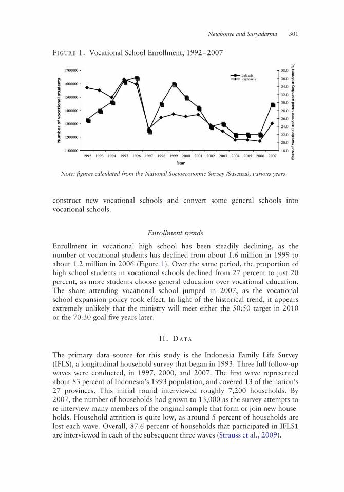
construct new vocational schools and convert some general schools intovocational schools.

Enrollment trends

Enrollment in vocational high school has been steadily declining, as thenumber of vocational students has declined from about 1.6 million in 1999 toabout 1.2 million in 2006 (Figure 1). Over the same period, the proportion ofhigh school students in vocational schools declined from 27 percent to just 20percent, as more students choose general education over vocational education.The share attending vocational school jumped in 2007, as the vocationalschool expansion policy took effect. In light of the historical trend, it appearsextremely unlikely that the ministry will meet either the 50:50 target in 2010or the 70:30 goal five years later.

I I . D A T A

The primary data source for this study is the Indonesia Family Life Survey(IFLS), a longitudinal household survey that began in 1993. Three full follow-upwaves were conducted, in 1997, 2000, and 2007. The first wave representedabout 83 percent of Indonesia’s 1993 population, and covered 13 of the nation’s27 provinces. This initial round interviewed roughly 7,200 households. By2007, the number of households had grown to 13,000 as the survey attempts tore-interview many members of the original sample that form or join new house-holds. Household attrition is quite low, as around 5 percent of households arelost each wave. Overall, 87.6 percent of households that participated in IFLS1are interviewed in each of the subsequent three waves (Strauss et al., 2009).

FIGURE 1. Vocational School Enrollment, 1992–2007

Note: figures calculated from the National Socioeconomic Survey (Susenas), various years


The sample is constructed as follows. We began with respondents who wereinterviewed at least once between the ages of 18 and 50, as a detailed edu-cation history is only available for respondents aged 50 or younger. Next, welimited our sample to individuals who were born between 1940 and 1980. Wethen dropped individuals who were never interviewed after they graduatedjunior secondary, as well as those who were full-time students when inter-viewed. We then dropped observations that did not report complete schoolinformation. Finally, to avoid identification based on functional form assump-tions, we restrict the sample to the region of common support (Heckman andVytlacil, 2001; Tobias, 2003). To do this, we estimated the probability thateach person either leaves the schooling system without graduating from seniorsecondary or attends each of the four school types using a multinomial logitmodel, and dropped observations for which the estimated probability ofattending public general school falls outside the range of all public generalgraduates. Finally, we dropped reported wages from the bottom and top per-centile from wage regressions to avoid distorted results due to outliers.Table S2.1 in Appendix S2 shows the number of observations that weredropped during each stage of this process.

After dropping observations outside the region of common support, the finalsample consists of 17,485 total labor market observations on 7,607 individ-uals. These individuals are divided into three cohorts. The oldest cohort con-sists of those born from 1940 to 1963, the middle cohort covers those bornfrom 1964 to 1972, and the youngest cohort contains those born from 1973 to1980. The IFLS survey asks the youngest cohort to report their performance inthe junior secondary final examination.12 Hence, for this most recent cohort, adirect measure of scholastic ability is available. Descriptive statistics for allvariables are given in Table S2.2 in Appendix S2.

All estimates are separated by sex, because men and women exhibit differentlabor market participation patterns and they select different education majors.According to the 2006 National Labor Force Survey (Sakernas), 64 percent ofmen choose a technical or industrial major, while 56 percent and 29 percent ofwomen are enrolled in business management and tourism majors, respectively.

I I I . U N D E R S T A N D I N G S C H O O L C H O I C E

To better understand the determinants of an individual’s school choice, we esti-mate the following multinomial logit regression:

Ti ¼ aZZi þ aiPi þ adPd þ 1i ð1Þ

where Ti is a five-category variable indicating senior secondary school type or

12. The examination is designed to be nationally comparable by the Ministry of National

Education. We standardize the scores by year of junior secondary graduation to take into account

possible quality changes in the exam over time.


non-graduation, Zi is a vector of predetermined characteristics, Pi is parentaleducation, and Pd is district-level parental education shares.

Table 1 provides the estimated marginal effects of selected independent vari-ables. It shows that the reduction in vocational enrollment observed in Figure 1resulted first in an increase in the probability of attending private school, andthen decreases in high school attendance. The top rows of the third columnshow that men in the middle and recent cohorts were 9.6 and 11.4 percentagepoints less likely to enroll in public vocational schools than those in the oldestcohorts. Men in the middle cohort were more likely to attend general school,by 9.6 percentage points, but private vocational school has become morepopular for men in the youngest cohort. Girls have also increasingly turnedaway from public vocational education. The probability of attending generaland vocational private schools both increased by 8.7 and 6.5 percentage pointsrespectively for the middle cohort. This increase in private general persisted forthe youngest cohort.

The table also shows that a higher percentage of men in the recent cohortleft without completing senior secondary education, compared to men in theold and middle cohort. To a certain extent, we find a similar pattern amongthe recent cohort of women. We believe that there are two plausible expla-nations for this pattern. First, the composition of junior high school graduateschanged, partly as a result of a nine-year compulsory education program thatwas enacted by the government in the early 1990s. This program caused somestudents to graduate from junior high school that would have dropped out inthe older cohorts, and these new junior high graduates were less likely to con-tinue on to high school.13 Second, the rapid increase in the supply of highschool graduates eroded the returns to completing high school. Turning to par-ental education, the children of highly educated parents are more likely toattend general schools. Increased paternal education raises the probability ofattending private general school the most, followed by public general schools.The pattern is similarly strong among women.

The Effect of Test Scores on School Choice

Test score data is available for the most recent cohort (those born between1973 and 1980). For this cohort, we examine how test scores relate to schoolchoice, and whether including test scores alters the estimated effect of the otherindependent variables, especially parental education. Table S3.1 in AppendixS3 provides the estimation results for men, while Table S3.2 shows the resultsfor women.

13. This generational shift from dropping out after completing primary school to dropping out after

junior secondary school would have been clearer had our sample consisted of all individuals, not just

those who completed junior secondary school. However, since our main interest is to describe the

choice of senior secondary education, we choose to continue using our current sample.


TA

BL

E1

.D

eter

min

ants

of

Sch

ool

Enro

llm

ent:

sele

cted

vari

able

s,fu

llsa

mple

Men

Wom

en

No

senio

rse

condary

Public

gen

eral

Public

voca

tional

Pri

vat

egen

eral

Pri

vat

evo

cati

onal

No

senio

rse

condary

Public

gen

eral

Public

voca

tional

Pri

vat

egen

eral

Pri

vat

evo

cati

onal

Per

sonal

chara

cter

isti

csM

iddle

Cohort

0.6

2.9

*2

9.6

***

6.7

***

20.7

29.7

***

2.4

27.9

***

8.7

***

6.5

***

(2.1

)(1

.7)

(1.7

)(1

.7)

(1.5

)(2

.4)

(2.2

)(2

.0)

(2.0

)(1

.7)

Rec

ent

cohort

12.8

***

24.5

***

211.4

***

20.8

4.0

**

3.9

0.6

212.2

***

2.9

*4.7

***

(2.2

)(1

.7)

(1.6

)(1

.7)

(1.6

)(2

.5)

(1.8

)(1

.8)

(1.8

)(1

.5)

Rep

eate

dgra

de

inju

nio

rse

condary

0.1

23.7

23.4

6.6

0.3

5.5

21.4

25.7

20.3

1.9

(4.4

)(4

.2)

(2.9

)(4

.8)

(3.7

)(8

.2)

(6.1

)(4

.8)

(8.0

)(5

.1)

Liv

edin

small

tow

nat

age

12

25.1

**

2.6

0.4

20.3

2.4

26.0

***

4.6

**

20.6

0.4

1.6

(2.1

)(1

.7)

(1.5

)(1

.6)

(1.7

)(2

.1)

(1.9

)(1

.6)

(1.7

)(1

.5)

Liv

edin

big

city

atage

12

26.5

**

7.2

***

20.2

23.2

*2.7

25.4

**

5.8

**

1.1

4.2

**

25.6

***

(2.6

)(2

.2)

(1.8

)(1

.8)

(2.1

)(2

.7)

(2.3

)(2

.1)

(2.1

)(1

.6)

Hei

ght

20.3

**

0.1

20.0

0.3

**

20.1

20.5

***

0.2

0.1

0.3

**

20.1

(0.1

)(0

.1)

(0.1

)(0

.1)

(0.1

)(0

.2)

(0.1

)(0

.1)

(0.1

)(0

.1)

Pare

nta

led

uca

tion

Fat

her

gra

duat

edel

emen

tary

213.7

***

6.1

**

1.6

5.7

***

0.3

215.4

***

2.3

1.1

6.8

***

5.2

*(3

.5)

(2.4

)(2

.3)

(2.1

)(2

.6)

(4.1

)(3

.1)

(2.8

)(2

.3)

(2.7

)Fat

her

gra

duat

edju

nio

rse

condary

224.6

***

10.1

***

1.6

12.1

***

0.9

228.7

***

7.5

**

1.3

11.3

***

8.6

***

(4.0

)(3

.1)

(2.8

)(3

.0)

(3.3

)(4

.7)

(3.6

)(3

.3)

(3.0

)(3

.2)

Fat

her

gra

duat

edse

nio

rse

condary

224.6

***

9.5

**

20.0

15.8

***

20.6

242.5

***

14.2

***

4.2

18.2

***

6.0

(5.7

)(3

.7)

(3.3

)(4

.0)

(3.9

)(5

.2)

(4.8

)(3

.8)

(4.1

)(3

.7)


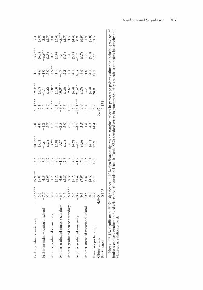
Fat

her

gra

duat

eduniv

ersi

ty2

27.6

***

19.9

***

24.6

18.1

***

25.8

240.1

***

19.4

***

1.7

13.7

***

5.3

(5.5

)(5

.0)

(3.5

)(5

.1)

(4.0

)(6

.1)

(5.7

)(4

.6)

(4.8

)(5

.0)

Fat

her

atte

nded

voca

tional

school

27.7

4.5

6.5

21.6

21.8

5.4

21.1

21.0

26.9

**

3.6

(5.6

)(3

.9)

(4.2

)(3

.3)

(3.7

)(5

.9)

(3.6

)(3

.0)

(2.8

)(3

.7)

Moth

ergra

duat

edel

emen

tary

22.2

1.7

22.7

3.9

*2

0.7

26.8

**

5.8

**

4.9

***

20.9

23.0

(2.7

)(2

.2)

(2.0

)(2

.0)

(2.1

)(3

.1)

(2.3

)(1

.7)

(2.4

)(2

.4)

Moth

ergra

duat

edju

nio

rse

condary

26.4

4.6

21.5

5.8

*2

2.5

28.8

**

10.9

***

20.7

4.3

25.7

**

(4.3

)(3

.3)

(2.8

)(3

.1)

(3.0

)(3

.8)

(3.0

)(2

.2)

(3.3

)(2

.7)

Moth

ergra

duat

edse

nio

rse

condary

218.1

***

9.5

*2

2.7

5.1

6.1

210.6

9.6

**

4.5

1.1

24.5

(5.5

)(5

.2)

(4.3

)(4

.9)

(5.7

)(6

.8)

(4.4

)(4

.1)

(5.1

)(4

.4)

Moth

ergra

duat

eduniv

ersi

ty2

0.8

11.6

21.9

24.1

24.7

231.1

***

21.6

**

10.5

21.7

0.8

(9.3

)(7

.9)

(7.6

)(4

.0)

(5.5

)(6

.6)

(8.7

)(8

.6)

(6.7

)(6

.9)

Moth

erat

tended

voca

tional

school

20.5

20.0

4.8

22.5

21.8

23.9

3.2

21.0

21.6

3.4

(8.3

)(4

.5)

(6.1

)(4

.2)

(4.3

)(7

.8)

(4.4

)(4

.1)

(5.0

)(5

.8)

Base

case

pro

babil

ity

34.8

19.7

13.3

17.9

14.4

35.9

20.0

13.1

17.5

13.5

Obse

rvat

ions

4,0

40

3,5

67

R2

Square

d0.1

03

0.1

24

Note

s:***

1%

signifi

cance

,**

5%

signifi

cance

,*

10%

signifi

cance

;figure

sare

marg

inal

effe

cts

inper

centa

ge

poin

ts;

esti

mat

ion

incl

udes

pro

vin

ceof

junio

rse

condary

gra

duat

ion

fixed

effe

cts

and

all

vari

able

slist

edin

Table

S2.2

;st

andard

erro

rsin

pare

nth

eses

,th

eyare

robust

tohet

erosk

edast

icit

yand

clust

ered

atsu

bdis

tric

tle

vel.


For both sexes, students with test scores in the top tercile are far more likelyto attend public schools. Moreover, private vocational schools attract thelowest scoring students. Including test scores does not alter the finding abovethat highly educated parents choose general schools over vocational schools,although the effects are less precisely estimated.

In sum, the probability that students enroll in public vocational schoolsdeclined substantially for the middle and youngest cohort. However, this doesnot seem to be caused by a decline in the quality of public vocational students,as high scoring students are still more likely to attend public schools. The morelikely cause is an increase in the number of private schools, particularly privatevocational schools, which have responded to the continued high demand forhighly educated workers (World Bank, 2011).

Two main household characteristics are associated with choice of schooltype: scholastic ability and parental education. With regards to the former,high scoring students choose public schools as their first preference, followedby private general school. For parental education, private general schoolsattract the sons of better-educated fathers, followed by public general schools.Private vocational schools act as a last resort; students who enroll in theseschools disproportionately scores in the bottom tercile and their parents areless well educated.

I V. L A B O R M A R K E T E F F E C T S O F V O C A T I O N A L E D U C A T I O N

We turn from the determinants of students’ school type to their subsequentlabor market experience. We examine four different outcomes: labor force par-ticipation (LFP), unemployment conditional on participation, formal sectorwork, and log of hourly wage.14 The reduced form model estimated is:

Yit ¼ bZZi þ bPPi þ bDDd þ bYYt þ bTTi þ 1it ð2Þ

where Yit is the labor market outcome of person i in year t. Zi and Pi, as inequation one, are defined as a vector predetermined individual characteristicsand parental education, while Dd is a set of indicators for district of juniorsecondary school. Yt is a vector of interview year dummies, and Ti is a vectorof categorical dummies of the senior secondary school types, including nosenior secondary, with public general excluded given that our main interest isin comparing the returns to general relative to vocational.15

The equation is estimated using double robust regression, which rebalancesthe sample by reweighting observations according to the inverse estimated

14. The wage of self-employed individuals is calculated using their average hourly profit. The

Statistics Indonesia urban price index is used to deflate 1993 wages, while IFLS price indices are used

for subsequent years.

15. We do not control for university attendance, which is partially determined by choice of school

type.


probability of attending the type of school that a person graduated from. Whilethis reweighting reduces precision, it makes the estimates more robust tonon-linear functional forms.

A key indicator to measure the effectiveness of this reweighting procedure isthe normalized difference between means of the observed control variables fordifferent school types, compared to general public graduates (Imbens andWooldridge, 2009). Reweighting greatly reduces the average of the normalizeddifference across the 42 control variables. The average normalized differencefalls by 66 percent for public vocational graduates, 80 percent for privategeneral graduates, and 95 percent for private vocational graduates.16 Thisindicates that the reweighting was effective.

To the best of our knowledge, a plausible instrument for school choice doesnot exist.17 As a result, the OLS results reported would be biased to the extentthat school choice is based on unobserved determinants of labor market out-comes.18 Non-random selection into employment will also bias the estimatedeffects of school type on formality and wages, if unobserved determinants ofschool type are correlated with the probability that different types of graduateschoose to work. It is therefore important to control for as many pre-determinedor exogenous characteristics as possible. Fortunately, the survey collects a largeamount of data on individual and family characteristics. We include parentaleducation, for both resident and non-co-resident parents; height; self-reportedsize of residence at age 12; grade repetition in junior high and elementaryschool; public lower secondary school attendance; working while attendingelementary school, or lower secondary, and year of interview. In addition, theyoungest cohort was asked to report their lower secondary test score, whichcan be used to gauge the bias due to omitting this variable. We include districtof junior secondary graduation fixed effects to take into account differences inthe supply of education, community characteristics, and peer effects that varyacross district.19 Finally, survey year and cohort dummies are included, whichcaptures age as well. Despite the inclusion of several observed characteristics,

16. After rebalancing, the normalized difference between public general and public vocational

graduates is 0.006. For private general and vocational, the normalized difference is 0.005 and 0.001

respectively.

17. We have tried several instruments, including the share of schools of each type and the leave-out

mean of enrolment in each school type in the district and year where a person graduates from junior

secondary school. While the latter is a strong instrument, it is unlikely to be valid, as variation in school

attendance patterns across communities is undoubtedly correlated with local labor market conditions.

The best candidate instrument would be data on historical school construction, as in Duflo (2001).

However, this information is unavailable, and the village censuses (Podes) show little change in the

local prevalence of different types of high schools across time. Therefore, we elected to abandon the

instrumental variables approach.

18. Unfortunately, it is difficult to speculate as to the direction of the bias, given the lack of data on

unobserved characteristics such as motivation or aspirations, and the presence of several control

variables in the model.

19. District of lower secondary school is highly collinear with district of secondary school, as less

than a quarter of the sample attended junior and senior secondary schools in different districts.


however, there are important unobserved characteristics that are omitted andwe do not claim that the results are causal.

Table 2 shows the estimated labor market effects of different school typesrelative to public general, while the full estimation results are in Table S4.2 inAppendix S4. For robustness, the fourth and fifth columns give the estimates ofaverage and median returns.20

For men, the results show a substantial public school wage premium. Privategeneral graduates earn nearly 25 percent less than public general graduates andprivate vocational students nearly 18 percent less. These penalties are substan-tial given that non-graduates earn 40 percent less. In contrast, differencesbetween public and vocational schools are much smaller. The estimates are suf-ficiently precise to rule out a public vocational premium, relative to publicgeneral, exceeding 16 percent. Differences between public general and voca-tional graduates are more apparent, however, when examining formality.21

Graduating from a vocational school is associated with about a 6 percentagepoint greater chance of working in a formal job.

For male graduates of private schools, the average wage penalty is similarfor vocational and general graduates, although general graduates face a largermedian wage penalty. Private general school graduates are also much less likelyto get a formal job than private vocational graduates. Compared to publicschool graduates, private general graduates are 5 percentage points less likelyto work in a formal job, but private vocational graduates are 5 percentagepoints more likely to. The results for private general graduates are particularlydisappointing, since private vocational graduates tend to have lower parentaleducation levels than private general graduates, and in the most recent cohort,lower test scores as well.

Among women, private general schools are also associated with reducedlabor force participation and formality rates compared with graduates of theother three school types. With regards to wages, meanwhile, public vocationalgraduates earn a wage premium of 16 percent. The wage estimates for femalesare less precise but can nonetheless rule out a public vocational wage premiumthat is greater than 30 percent. Private general graduates earn the least com-pared to observable similar graduates of the other three schools, although thedifference is not statistically significant. As with men, women with no seniorsecondary education earn far less than those who attend senior secondary.

20. Although median regression is more robust to outliers, it does not allow for the inclusion of

district fixed effects. As a result, we included provincial rather than district effects in the median

regression specification.

21. A job is classified as formal if the worker is a salaried employee, is self-employed with

permanent workers, or is self-employed with temporary workers outside of agriculture. This definition,

which is based on employment status and sector, is 99 percent correlated with the official definition

adopted by the Statistics Indonesia, which is based on employment status and occupation. Formal

employees tend to earn higher wages and express greater job satisfaction than informal employees,

particularly casual workers (World Bank, 2011).


TA

BL

E2

.T

he

Eff

ect

of

Sch

ool

Types

on

Labor

Mark

etO

utc

om

es:

Full

sam

ple

poole

d

Men

Wom

en

LFP

Unem

plo

ymen

tForm

al

Wage

Wage

LFP

Unem

plo

ymen

tForm

al

Wage

Wage

LPM

LPM

LPM

OL

SL

AD

LPM

LPM

LPM

OL

SL

AD

No

seco

ndary

school

20.0

01

0.0

05

20.0

96***

20.4

04***

20.4

81***

20.1

47***

20.0

15

20.2

13***

20.4

73***

20.6

36***

(0.0

09)

(0.0

09)

(0.0

27)

(0.0

53)

(0.0

37)

(0.0

27)

(0.0

09)

(0.0

31)

(0.0

93)

(0.0

62)

Public

Voca

tional

0.0

15**

20.0

07

0.0

62**

0.0

41

0.0

07

0.0

29

20.0

20*

0.0

87***

0.1

58**

0.1

43***

(0.0

07)

(0.0

12)

(0.0

27)

(0.0

57)

(0.0

37)

(0.0

30)

(0.0

11)

(0.0

28)

(0.0

72)

(0.0

49)

Pri

vat

egen

eral

0.0

14*

20.0

04

20.0

50*

20.1

46**

20.2

48***

20.0

78**

0.0

17

20.0

84**

20.1

38

20.2

51***

(0.0

08)

(0.0

09)

(0.0

30)

(0.0

60)

(0.0

55)

(0.0

31)

(0.0

11)

(0.0

41)

(0.0

91)

(0.0

79)

Pri

vat

evo

cati

onal

0.0

06

0.0

04

0.0

48*

20.1

77***

20.1

76***

20.0

34

0.0

07

0.0

05

20.0

39

20.0

92

(0.0

08)

(0.0

12)

(0.0

28)

(0.0

60)

(0.0

35)

(0.0

31)

(0.0

12)

(0.0

41)

(0.0

90)

(0.0

71)

Ave

rage

am

ong

public

gen

eral

gra

duat

es0.9

71

0.0

53

0.7

12

0.6

98

0.0

43

0.7

34

R-s

quar

ed0.0

69

0.1

53

0.1

81

0.2

19

0.1

56

0.2

11

0.2

39

0.3

12

Obse

rvat

ions

9,0

12

8,7

74

8,3

42

7,3

70

7,3

70

8,4

73

5,1

36

4,9

28

3,8

01

3,8

01

Note

s:***

1%

signifi

cance

,**

5%

signifi

cance

,*

10%

signifi

cance

;st

andard

erro

rsin

pare

nth

eses

,th

eyare

robust

tohet

erosk

edast

icit

yand

clust

ered

atsu

bdis

tric

tle

vel;

LPM

stands

for

Lin

ear

Pro

babilit

yM

odel

,O

LS

stands

for

Ord

inary

Lea

stSquare

s,and

LA

Dfo

rL

east

Abso

lute

Dev

iati

ons.

Inall

case

s,th

esa

mple

isre

bala

nce

dby

rew

eighti

ng

obse

rvat

ions

by

the

esti

mat

edin

vers

epro

babilit

yof

atte

ndin

gth

eir

school

type,

inaddit

ion

tost

andard

indiv

idual

cross

-sec

tional

wei

ghts

.R

obust

standard

erro

rsare

report

ed.

All

esti

mat

esare

base

don

equat

ion

(2)

inth

ete

xt.

Wage

LA

Des

tim

ates

incl

ude

pro

vin

cial

inst

ead

of

dis

tric

tfixed

effe

cts.

Sta

ndard

erro

rsfo

rL

AD

esti

mat

esare

obta

ined

from

an

unw

eighte

dboots

trap

pro

cedure

.


One potential source of bias stems from the lack of a direct measure of scho-lastic ability for the entire sample. To assess the extent to which this omissiongenerates biased estimates of the returns to different types of schools, inTable S4.1 in Appendix S4 we include test scores in the estimation results usingthe youngest cohort and compare them to the results when the variable isexcluded. The results show, reassuringly, that the omission of test scores is anegligible source of bias.

V. H E T E R O G E N E I T Y I N A G E A N D C O H O R T

Returns to vocational education may decline over time. This could occur, forexample, if the specific skills taught in vocational schools become obsoletefaster than general skills. Vocational graduates’ specific skills may also enablethem to work immediately at a market wage after graduation, while generalgraduates need to be trained further by the firms that employ them. Over time,however, general graduates may find it easier to upgrade their skills to cater toemployers’ demands. In either case, vocational education would confer aninitial advantage that would erode over time.

In this section, we examine age effects for different cohorts, which enable usto separate age effects from cohort effects. There has been little research exam-ining how the returns to school type vary by age in developing counties, largelydue to the lack of long-running longitudinal datasets. As we discuss in SectionIII, we divided the IFLS sample into three cohorts: old (those born between1940 and 1962), middle (1963 – 1972), and young (1973 – 1980). For eachcohort, we estimate the following equation:

Yit ¼ bZZi þ bPPi þ bDDd þ bYYt þ bTTi þ bty Ti � Ytð Þ þ 1it ð3Þ

In this specification, bty is a 1 X 16 vector, containing the estimated effect ofeach school type, relative to public general, for each of the four survey waves.We discuss the outcomes in turn below, while the graphic representation andestimation results are in Appendix S5.22

We begin by looking at the effect of vocational school on labor force partici-pation, starting with men. Comparing the young and the middle cohorts, therecent cohort of men is more likely than the middle cohort to participate earlyin their career, although the difference is not statistically significant and disap-pears by age thirty. In general, the effect of public vocational education on

22. We graph these estimated effects, separately for each cohort, on the vertical axis. The horizontal

axis represents the average age of each cohort in the relevant year. Therefore, for each cohort and labor

market indicator, there are four estimates of the effect, spanning fourteen years of the cohort’s life.

Since the youngest cohort covers those born from 1973 to 1980, its oldest members were 20 in 1993.

Since only a few members of the youngest cohort were working in 1993, these estimates are not

reported. We also calculate the effect for private general and private vocational schools. However,

because the vocational expansion in prioritising public vocational over public general, in this section we

focus on these two school types.


participation is approximately one and a half percentage points, which issizable given that only three percent of male public general graduates, onaverage, do not participate in the labor force. The positive effect of publicvocational school on participation begins to decline at age thirty and becomesnegative around the age of forty.

The pattern for women, shown in Figure S5.2, is the opposite. The positiveeffect of public vocational on participation starts high, declines, and thenrecovers. The five percentage premium experienced by 25 year-olds decreaseswith age, reaches a bottom of negative percentage points in the early 30s, andthen increases to ten percentage points for older women. There are no apparentcohort effects.

Turning to the probability of unemployment, the difference in unemploy-ment between public general and public vocational graduates is shown inFigure S5.3 for men and Figure S5.4 for women. Men exhibit no cohorteffects, as the graph is continuous across cohorts. Public vocational graduatesenjoy lower unemployment from their early twenties until they turn thirty.After that, the effect of vocational education remains close to zero withoutbecoming statistically significant.

For females, meanwhile, there is a sizeable cohort effect between the youngand the middle cohorts. At the age of twenty-five, vocational graduates in theyoung cohort enjoy lower unemployment rates than general graduates, whilevocational graduates in the middle cohort face the same unemployment rate asgeneral graduates. At around thirty, however, the unemployment rate of voca-tional graduates in the young cohort is higher than general graduates. Lookingat the age profile, it appears that general and vocational graduates over thirtyyears old have similar unemployment rates.

Next, Figure S5.5 examines the effect of public vocational education on theprobability of holding a formal job, conditional on being employed. For themiddle cohort in 1993, when their average was 26, public vocational graduatesenjoyed a large formality premium of nearly 30 percentage points, whichgradually declined to 10 percentage points in 2007. That formality premium,disappeared for the younger cohort, however. In the year 2000, when theiraverage age was 23, the formality premium for the youngest cohort was 5 per-centage points and seven years later it was essentially zero.

For female public vocational graduates, unlike their male counteparts, thereis no evidence of a fall in the formality premium for the youngest cohort.Figure S5.6 shows that female public vocational graduates are no more likelyto work in formal jobs than public general graduates from ages 20 to 30. Afterage 30, public vocational graduates are slightly more likely to be in a formaljob, but that formality premium gradually declines.

The last labor market outcome that we examine is the reported wage, shownin Figures 2 and 3. The comparison between the middle and youngest cohort isparticularly striking. In the middle cohort, public vocational graduates enjoyedan estimated 40 percent wage premium in 1993, when they were 25, which


declined to essentially zero in 1997, 2000, and 2007. Male public vocationalgraduates in the youngest cohort, however, experienced a large wage penalty.The estimated penalty was 20 percent in 2000, when the cohort on averagewas 23, and 40 percent seven years later.

As was the case for informality, there is no clear sign of a cohort effect forwomen. The public vocational wage premium for the youngest cohort, whichwas 60 percent for women in 2007, if anything rose compared to the middlecohort. However, the estimates are imprecise and not statistically significant.Overall, the age-wage profile suggests a short-lived benefit for female voca-tional graduates in their mid to late twenties, which largely disappears in theirthirties before picking up again in their forties and fifties. The large publicvocational premium for the oldest cohort around the age of fifty is the onlyestimated effect that is statistically significant.

This section highlights the importance of estimating both cohort and ageeffects and treating age effects carefully. In general, the strongest effects of

FIGURE 2. Effect of Public Vocational on Wages, Men

Note: estimation results are in Table S5.4 in Appendix S5

FIGURE 3. Effect of Public Vocational on Wages, Women

Note: estimation results are in Table S5.4 in Appendix S5


vocational education are experienced early in life, between the ages of 20 and35. For example, while Table 2 shows an insignificant negative effect of voca-tional education on unemployment over the entire sample, results in thissection show that this effect is concentrated among young graduates in theirtwenties. Results for graduates younger than 25, however, are contaminated byuniversity enrollment decisions. This is because full time students are notincluded in the sample, and students typically do not typically graduate fromuniversity until age 25. University enrollment could explain part of the negativeeffect of vocational education on unemployment, for example. General second-ary school graduates are more likely to attend university than vocational gradu-ates, and university graduates are more likely to experience spells ofunemployment as they search for the best job following graduation. Since thedeterminants of university enrollment and graduates’ job search patterns arenot well understood and likely depend on unobserved factors, we focus onresults for groups over 25.

The results for recent graduates, particularly those between 25 and 35,suggest that the returns to public vocational school have declined sharply formen. For example, while Table 2 shows a higher formality rate among all malevocational graduates, Figure V.5 shows that the middle cohort drives this posi-tive formality rate in their youth, and that the premium has disappeared for theyoungest cohort. This is consistent with the dramatic fall in the effect of voca-tional education on men’s wages. Figure 2 shows that while workers in themiddle cohort enjoy a large vocational wage premium before they turn 30,individuals in the youngest cohort enjoy no such benefit. In contrast, afterenjoying a smaller wage premium at the age of 21, individuals in this cohortface an increasingly large wage penalty. Although male public vocationalgraduates face increasingly worse labor market outcomes, there is no sign of asimilar deterioration for female public vocational graduates.

One possible explanation for this decline for men relates to recent changesin the structure of the Indonesian economy. Since the financial crisis of 1998,the economy has increasingly relied on the service sector to generate growth.Annual growth in the industrial sector fell dramatically, from nine percentfrom 1990 to 1997, to four from 1999 to 2007. During the same two periods,annual service sector growth remained strong, falling slightly from seven to six.More recently, employment in the service sector has grown rapidly. From 2003to 2007, service sector employment grew at roughly four percent per yearwhile industrial sector employment grew at 2.5 percent per year (World Bank,2011). The increasing prominence of the service sector could disproportio-nately affect vocationally trained males because they tend to choose technicalmajors. Women, on the other hand, tend to choose to study business manage-ment or tourism skills, for which demand may have remained stronger. In anincreasingly service-oriented economy, there may be decreased demand for theindustrial and technical majors chosen by most men in vocational schools.


Another potential explanation for the recent decline in male vocationalreturns is deterioration in the quality of vocational training for men. Forexample, technical vocational training may require larger investments toremain relevant to new advances in technology. Unfortunately, it is difficult toinvestigate this further, due to the lack of data on trends in the quality ofindustrial education facilities.

V I . H E T E R O G E N E I T Y I N F A M I L Y B A C K G R O U N D

The second aspect of heterogeneity that we examine is family background,proxied for by father’s education. We separate the sample into two categories:those whose father has at most a junior secondary education and those whosefather has at least a senior secondary education. Table 3 shows the estimationresults for men. Comparing the results with the ones in Table 2, we find thatthe effects of school types on labor market outcomes are mostly limited to stu-dents from a disadvantaged background. Among these individuals, graduatesof public vocational schools have a higher formality rate than public generalschool graduates, while private general graduates face the lowest prospects of aformal job. In addition, private school graduates face a large wage penalty rela-tive to public school graduates. In short, public schools appear to provide themost benefit for children from disadvantaged families.

The estimation results for women, shown in Table 4, give similar con-clusions. The labor market effects of school types are for the most part onlysignificant among those coming from a disadvantaged background, except theformality penalty among private general graduates. Among individuals fromdisadvantaged background, private general graduates fare the worst, facing alower participation and job formality rate. In contrast, public vocational gradu-ates have the highest labor force participation and formality rate.

V I I . H E T E R O G E N E I T Y I N AC A D E M I C A B I L I T Y

The final aspect of heterogeneity in the labor market effects of different schooltypes that we consider pertains to academic ability. Does higher ability mitigateor magnify the labor market effects of school types?23 Since test scores are onlyavailable for the youngest cohort, the relevant benchmarks are given inTable IV.1 in Appendix S4, which shows that recent male private general andpublic vocational graduates experience a substantial wage penalty.

Table 5 provides the estimated effects of school type for men that scoredabove and below the median on their junior high exit exam. For men scoringbelow the mean, public vocational education is much more likely to lead to aformal job, but the average wage is much lower. Interestingly, private

23. Note that our sample is rebalanced and has common support over the test score distribution,

which allows for valid comparisons across school types despite large differences in average test scores.


TA

BL

E3

.E

stim

ated

Eff

ect

of

Sch

ool

Type

on

Em

plo

ymen

tand

Job

Quality

,M

en,

by

fath

er’s

educa

tion

Junio

rse

condary

or

bel

ow

Sen

ior

seco

ndary

or

above

LFP

Unem

plo

ym

ent

Form

al

Wage

LFP

Unem

plo

ym

ent

Form

al

Wage

LPM

LPM

LPM

OL

SL

PM

LPM

LPM

OL

S

No

senio

rse

condary

20.0

01

0.0

08

20.1

31***

20.4

81***

20.0

26

0.0

24

20.0

08

20.1

71

(0.0

08)

(0.0

08)

(0.0

29)

(0.0

52)

(0.0

26)

(0.0

42)

(0.0

74)

(0.2

14)

Public

voca

tional

0.0

02

20.0

11

0.0

62**

0.0

37

0.0

23

0.0

16

0.0

11

0.0

23

(0.0

06)

(0.0

09)

(0.0

30)

(0.0

59)

(0.0

15)

(0.0

30)

(0.0

53)

(0.1

33)

Pri

vat

egen

eral

0.0

06

20.0

09

20.0

66**

20.2

30***

0.0

45**

0.0

08

0.0

17

20.1

22

(0.0

08)

(0.0

08)

(0.0

30)

(0.0

58)

(0.0

18)

(0.0

27)

(0.0

53)

(0.1

56)

Pri

vat

evo

cati

onal

20.0

02

0.0

11

0.0

02

20.2

81***

0.0

02

0.0

70*

0.0

49

20.1

10

(0.0

08)

(0.0

13)

(0.0

28)

(0.0

70)

(0.0

27)

(0.0

39)

(0.0

69)

(0.1

35)

Ave

rage

am

ong

publi

cgen

eral

gra

duat

es0.9

72

0.0

44

0.7

58

0.9

61

0.0

67

0.8

14

R-s

quare

dove

rall

0.0

59

0.1

51

0.1

86

0.2

31

0.1

69

0.3

18

0.3

28

0.4

03

Obse

rvat

ions

6,6

50

6,4

89

6,2

01

5,4

81

1,2

14

1,1

64

1,0

63

928

Note

s:***

1%

signifi

cance

,**

5%

signifi

cance

,*

10%

signifi

cance

;st

andard

erro

rsin

pare

nth

eses

,th

eyare

robust

tohet

erosk

edast

icit

yand

clust

ered

atsu

bdis

tric

tle

vel.


TA

BL

E4

.E

stim

ated

Eff

ect

of

Sch

ool

Type

on

Em

plo

ymen

tand

Job

Quality

,W

om

en,

by

fath

er’s

educa

tion

Junio

rse

condary

or

bel

ow

Sen

ior

seco

ndary

or

above

LFP

Unem

plo

ym

ent

Form

al

Wage

LFP

Unem

plo

ym

ent

Form

al

Wage

LPM

LPM

LPM

OL

SL

PM

LPM

LPM

OL

S

No

senio

rse

condary

20.1

19***

20.0

24*

20.2

40***

20.5

67***

20.1

18*

20.0

21

20.0

50

20.0

48

(0.0

29)

(0.0

13)

(0.0

34)

(0.0

98)

(0.0

63)

(0.0

39)

(0.1

09)

(0.1

51)

Public

voca

tional

0.0

69**

20.0

16

0.0

57*

0.1

69*

0.0

54

20.0

39

0.0

25

20.0

27

(0.0

32)

(0.0

13)

(0.0

33)

(0.0

90)

(0.0

62)

(0.0

27)

(0.0

61)

(0.1

32)

Pri

vat

egen

eral

20.0

68**

20.0

01

20.1

22***

20.2

72**

20.0

33

0.0

01

20.1

25**

0.1

25

(0.0

33)

(0.0

14)

(0.0

44)

(0.1

37)

(0.0

54)

(0.0

32)

(0.0

62)

(0.1

40)

Pri

vat

evo

cati

onal

20.0

20

0.0

11

20.0

38

20.0

30

20.0

70

20.0

01

20.0

72

0.1

88

(0.0

37)

(0.0

16)

(0.0

42)

(0.0

98)

(0.0

86)

(0.0

33)

(0.0

72)

(0.1

64)

Ave

rage

am

ong

publi

cgen

eral

gra

duat

es0.6

40

0.0

50

0.7

11

0.7

00

0.0

73

0.8

15

R-s

quare

dove

rall

0.1

46

0.2

01

0.2

57

0.3

38

0.2

70

0.3

25

0.3

71

0.4

42

Obse

rvat

ions

5,9

96

3,5

64

3,4

35

2,5

86

1,5

69

1,0

30

969

804

Note

s:***

1%

signifi

cance

,**

5%

signifi

cance

,*

10%

signifi

cance

;st

andard

erro

rsin

pare

nth

eses

,th

eyare

robust

tohet

erosk

edast

icit

yand

clust

ered

atsu

bdis

tric

tle

vel.


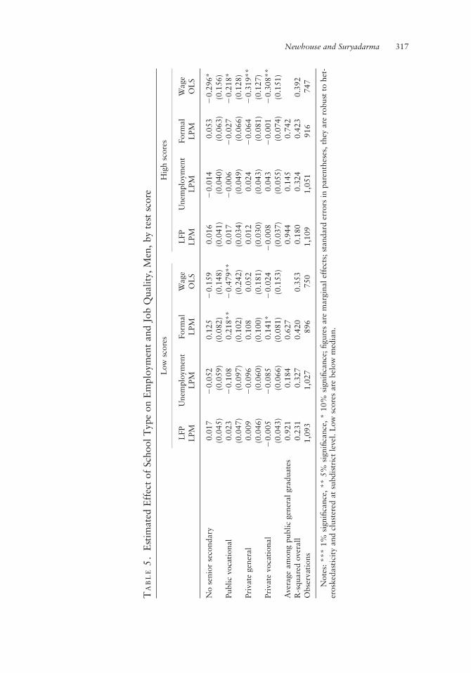
TA

BL

E5

.E

stim

ated

Eff

ect

of

Sch

ool

Type

on

Em

plo

ymen

tand

Job

Quality

,M

en,

by

test

score

Low

score

sH

igh

score

s

LFP

Unem

plo

ym

ent

Form

al

Wage

LFP

Unem

plo

ym

ent

Form

al

Wage

LPM

LPM

LPM

OL

SL

PM

LPM

LPM

OL

S

No

senio

rse

condary

0.0

17

20.0

52

0.1

25

20.1

59

0.0

16

20.0

14

0.0

53

20.2

96*

(0.0

45)

(0.0

59)

(0.0

82)

(0.1

48)

(0.0

41)

(0.0

40)

(0.0

63)

(0.1

56)

Public

voca

tional

0.0

23

20.1

08

0.2

18**

20.4

79**

0.0

17

20.0

06

20.0

27

20.2

18*

(0.0

47)

(0.0

97)

(0.1

02)

(0.2

42)

(0.0

34)

(0.0

49)

(0.0

66)

(0.1

28)

Pri

vat

egen

eral

0.0

09

20.0

96

0.1

08

0.0

52

0.0

12

0.0

24

20.0

64

20.3

19**

(0.0

46)

(0.0

60)

(0.1

00)

(0.1

81)

(0.0

30)

(0.0

43)

(0.0

81)

(0.1

27)

Pri

vat

evo

cati

onal

20.0

05

20.0

85

0.1

41*

20.0

24

20.0

08

0.0

43

20.0

01

20.3

08**

(0.0

43)

(0.0

66)

(0.0

81)

(0.1

53)

(0.0

37)

(0.0

55)

(0.0

74)

(0.1

51)

Ave

rage

am

ong

publi

cgen

eral

gra

duat

es0.9

21

0.1

84

0.6

27

0.9

44

0.1

45

0.7

42

R-s

quare

dove

rall

0.2

31

0.3

27

0.4

20

0.3

53

0.1

80

0.3

24

0.4

23

0.3

92

Obse

rvat

ions

1,0

93

1,0

27

896

750

1,1

09

1,0

51

916

747

Note

s:***

1%

signifi

cance

,**

5%

signifi

cance

,*

10%

signifi

cance

;figure

sare

marg

inal

effe

cts;

standard

erro

rsin

pare

nth

eses

,th

eyare

robust

tohet

-er

osk

edast

icit

yand

clust

ered

atsu

bdis

tric

tle

vel.

Low

score

sare

bel

ow

med

ian.


vocational school is also associated with an increase in formality, and has noassociated penalty.

For men scoring above the median, the results illustrate the benefits ofattending public general school. Public general graduates earn a 20 percentpremium over public vocational students and a 30 percent premium overprivate school graduates. Remarkably, there appears to be no positive return toattending private school, relative to not graduating, for high scoring men. It isthese high scoring men who stand the most to lose from attending vocationalor lower-quality private general education in an economy that increasinglyvalues broadly educated and cognitively skilled workers.

The results for women are shown in Table 6. Most striking are the differenteffects of school type on wages for low and high scoring women. Unlike formen, high-scoring women face no major wage penalty for attending publicvocational or private general school. The wage penalty for private vocationalschool, relative to public general, is 35 percent, and nearly equal to the penaltyfor not graduating high school. For low scoring women, there is suggestive evi-dence that vocational school helps. Low scoring women who attend public andprivate vocational schools earn approximately a 38 percent and 30 percentwage premium, respectively. Although not statistically significant, these arelarge premiums.

V I I I . C O N C L U S I O N

This paper attempts to better understand the determinants of households’choice of senior secondary schools in Indonesia and the labor market conse-quences of attending different types of high schools. This is the first paper toour knowledge from a developing country that distinguishes between publicand privately provided vocational schools, to assess whether private vocationalschools impart skills more relevant to a rapidly changing labor market.Another key contribution is a careful examination of heterogeneity in theeffects. We examine effects separately by age, cohort, parental education, andability. The use of longitudinal data allows for cohort effects to be distin-guished from age effects. Finally, the estimation utilizes an unusually rich set ofpredetermined control variables. While the possibility of bias due to unob-served characteristics cannot be dismissed, it is reassuring that for the youngestcohort, the inclusion of test scores – the most important determinant of schooltype – does not significantly alter the results.

The two most important observed determinants of school choice are testscores and parental education. Students with high test scores are most likely toattend public schools, particularly public general school. In contrast, the chil-dren of highly educated parents tend to select general schools, particularlyprivate general, rather than vocational schools. Private vocational school is alast resort, serving students with the lowest test scores and the least educatedparents.


TA

BL

E6

.E

stim

ated

Eff

ect

of

Sch

ool

Type

on

Em

plo

ymen

tand

Job

Quality

,W

om

en,

by

test

score

Low

score

sH

igh

score

s

LFP

Unem

plo

ym

ent

Form

al

Wage

LFP

Unem

plo

ym

ent

Form

al

Wage

LPM

LPM

LPM

OL

SL

PM

LPM

LPM

OL

S

No

senio

rse

condary

20.0

78

0.0

51

20.2

69***

0.0

51

20.0

64

20.1

01**

20.1

55**

20.3

76**

(0.0

71)

(0.0

50)

(0.1

02)

(0.3

01)

(0.0

62)

(0.0

50)

(0.0

73)

(0.1

66)

Public

voca

tional

0.0

08

0.0

70

20.2

08

0.3

83

20.0

16

20.0

71*

0.0

70

20.0

81

(0.0

95)

(0.0

70)

(0.1

33)

(0.3

89)

(0.0

64)

(0.0

39)

(0.0

86)

(0.1

54)

Pri

vat

egen

eral

20.0

72

0.1

02

20.1

68

0.1

48

20.0

32

20.0

31

20.1

20

0.0

12

(0.0

87)

(0.0

74)

(0.1

21)

(0.3

48)

(0.0

81)

(0.0

59)

(0.0

90)

(0.1

60)

Pri

vat

evo

cati

onal

0.0

08

0.1

17*

20.1

22

0.3

01

20.0

07

0.0

37

0.0

43

20.3

51*

(0.0

87)

(0.0

66)

(0.1

12)

(0.2

92)

(0.0

64)

(0.0

69)

(0.0

71)

(0.1

91)

Ave

rage

am

ong

publi

cgen

eral

gra

duat

es0.5

69

0.0

60

0.6

72

0.6

89

0.1

56

0.7

67

R-s

quare

dove

rall

0.2

39

0.4

02

0.4

84

0.5

48

0.3

24

0.3

81

0.4

34

0.5

06

Obse

rvat

ions

1,2

19

680

624

437

1,1

69

774

692

525

Note

s:***

1%

signifi

cance

,**

5%

signifi

cance

,*

10%

signifi

cance

;figure

sare

marg

inal

effe

cts;

standard

erro

rsin

pare

nth

eses

,th

eyare

robust

tohet

-er

osk

edast

icit

yand

clust

ered

atsu

bdis

tric

tle

vel.

Low

score

sare

bel

ow

med

ian.


With regard to labor market outcomes, we find a striking distinctionbetween publicly and privately schooled men. Male private school graduates,compared to their public school counterparts, suffer an average wage penaltyof approximately 16 percent. This large wage penalty is robust to medianregression. For men with high test scores, the correlation between publicgeneral attendance and subsequent wages is particularly strong. The patternsare somewhat different for women. Public school graduates earn more thanprivate general graduates, but there are important differences between types ofgraduates.

Among employed public school graduates, vocational graduates have tra-ditionally fared slightly better than general graduates in the labor market,although this is no longer the case among men. In general, attending publicvocational school attendance has a mild, positive, and statistically insignificantcorrelation with wages, and the estimates are sufficiently precise to rule outwage effects greater than 16 percent for men. Public vocational schoolsincrease the probability of obtaining a formal job, as defined by the IndonesianBureau of Statistics, by six percentage points. For women, the results suggest apositive effect of public vocational education, although this effect is onlyclearly discernible for the oldest cohort of women. There is suggestive evidencethat this positive effect of public vocational school is strongest for women withlower test scores. In contrast to men, the outcomes for female public vocationalgraduates in recent years have, if anything, improved.

The most dramatic result, which comes from disentangling age and cohorteffects, is the large drop in the wage premium for the most recent cohort ofmale public vocational graduates. This drop is unlikely to be explained bychanges in the unobserved characteristics of vocational graduates, as there areno major changes in the observed characteristics of vocational attendance forthe youngest cohort. While we cannot directly explore the underlying causesbehind this drop, plausible possibilities include a fall in the educational qualityof the technical and industrial majors favored by men, as well as the decliningrelevance of these skills in an increasingly service-oriented Indonesianeconomy.

In sum, the results suggest that whether high schools are publicly or pri-vately administered and whether the curriculum is vocational or general areboth important factors influencing graduates’ subsequent labor market out-comes. Male private school graduates earn substantially less than their publiclyschooled peers. Private general school graduates perform particularly poorly,despite their parents’ higher education levels. This highlights the need forfurther research to investigate the importance of peer effects, curriculum, tea-chers, and reputation effects in explaining these results. The current evidence isinsufficient to justify a recommendation to rapidly expand access to publicschools. Nonetheless, given the especially strong results for men with high testscores, a logical first step would be ensuring access to public general schoolsfor these high-scoring students.


Most importantly, the analysis provides little evidence to support the currentexpansion of vocational education, especially for men. The results fail to showsystematic benefits for public vocational graduates compared to public generalgraduates, despite reasonably precise estimates. Furthermore, the wage penaltyfor male vocational graduates, in recent years, has increased dramatically. Thedecline has occurred as Indonesia’s industrial sector has sharply slowed and theservice sector has become increasingly important to economic growth.Therefore, the general equilibrium effects of a large increase in the supply ofvocational graduates should further magnify the wage penalty that we observein this partial equilibrium investigation. This suggests that it may be worth-while to review, and possibly reform, vocational and technical education inmale-dominated subjects.

RE F E R E N C E S

Bennell, Paul. 1996. “General versus Vocational Secondary Education in Developing Countries: A

Review of the Rates of Return Evidence.” Journal of Development Studies, 33(2): 230–247.

Bennell, Paul, and Jan Segerstrom. 1998. “Vocational Education and Training in Developing Countries:

Has the World Bank Got it Right?” International Journal of Educational Development, 18(4):

271–287.

Chen, Dandan. 2009. Vocational Schooling, Labor Market Outcomes, and College Entry. Policy

Research Working Paper 4814. Washington, DC: World Bank.

Duflo, Esther. 2001. “Schooling and Labor Market Consequences of School Construction in Indonesia:

Evidence from an Unusual Policy Experiment”, American Economic Review, 91(4): 795–813

El-Hamidi, Fatma. 2006. “General or Vocational Schooling? Evidence on School Choice, Returns, and

‘Sheepskin’ Effects from Egypt 1998.” Journal of Policy Reform, 9(2): 157–176.

Ghozali, Abbas. 2006. Analisis Biaya Satuan Pendidikan Dasar dan Menengah. Jakarta. mimeo.

Heckman, James J., and Edward Vytlacil. 2001. “Identifying the Role of Cognitive Ability in

Explaining the Level of and Change in the Return of Schooling.” Review of Economics and

Statistics, 83(1): 1–12.

Horowitz, Andrew W., and Christoph Schenzler. 1999. “Returns to General, Technical and Vocational

Education in Developing Countries: Recent Evidence from Suriname.” Education Economics, 7(1):

5–19.

Imbens, Guido, and Jeffrey Woolridge, 2009, “Recent Developments in the Econometrics of Program

Evaluation.” Journal of Economic Literature, 47(1): 5–86

Jimenez, Emmanuel, Marlaine E. Lockheed, and Vicente Paqueo. 1991. “The Relative Efficiency of

Private and Public Schools in Developing Countries.” World Bank Research Observer, 6(2):

205–218.

Kahyarara, Godius, and Francis Teal. 2008. “The Returns to Vocational Training and Academic

Education: Evidence from Tanzania.” World Development, 36(11): 2223–2242.

KRIVET. 2008. Pre-employment Vocational Education and Training in Korea. mimeo.

Lechner, Michael. 2000. “An Evaluation of Public-Sector-Sponsored Continuous Vocational Training

Programs in East Germany.” Journal of Human Resources, 35(2): 347–375.

Malamud, Ofer, and Cristian Pop-Eleches. 2008. General Education vs. Vocational Training: Evidence

from an Economy in Transition. NBER Working Paper 14155. Cambridge, MA: National Bureau of

Economic Research.


Ministry of National Education. 2006. Rencana Strategis Departemen Pendidikan National Tahun

2005–2009. Jakarta: Ministry of National Education.

Moenjak, Thammarak, and Christopher Worswick. 2003. “Vocational education in Thailand: a study

of choice and returns.” Economics of Education Review, 22:99–107.

Neuman, Shoshana, and Adrian Ziderman. 1991. “Vocational Schooling, Occupational Matching, and

Labor Market Earnings in Israel.” Journal of Human Resources, 26(2): 256–281.

Newhouse, David, and Kathleen Beegle. 2006. “The Effect of School Type on Academic Achievement.”

Journal of Human Resources, 41(3): 529–557.

Strauss, John, Firman Witoelar, Bondan Sikoki, and Anna Marie Wattie. 2009. The Fourth Wave of the

Indonesia Family Life Survey: Overview and Field Report Volume 1. RAND Labor and Population

Working Paper WR-675/1-NIA/NICHD. Santa Monica, CA: RAND.

Tobias, Justin L. 2003. “Are Returns to Schooling Concentrated among the Most Ables? A

Semiparametric Analysis of the Ability-earnings Relationships.” Oxford Bulletin of Economics and

Statistics, 65(1): 1–29.

World Bank. 2011. Indonesia Jobs Report. Jakarta: World Bank.

———. 2007. Investing in Indonesia’s Education: Allocation, Equity and Efficiency of Public

Expenditures. Jakarta: World Bank.

———. 1995. Training and the Labor Market in Indonesia: Policies for Productivity Gains and

Employment Growth. Washington, DC: World Bank.


Disability and Poverty in Vietnam

Daniel Mont and Nguyen Viet Cuong

Disability is significantly correlated with poverty in Vietnam, according to data fromthe 2006 Vietnam Household Living Standards Survey, especially when the extra costsof living with a disability are taken into account. This disability-poverty link is alsoassociated with lower educational attainment, an important factor in determiningpoverty and productive economic activity in general, both for household-basedbusinesses and wage employment. Not taking into account these associations and theextra costs of disability will make some poor disabled people invisible in poverty stat-istics and impede efforts to reduce poverty. JEL codes: I12, I31, O15

Disability and poverty are linked in developing countries (Braithwaite andMont 2009; Fujii 2008; Mete 2008; Hoogeveen 2005; Yeo and Moore2003; Elwan 1999). However, quantitative research in this area is usuallyhampered by the lack of good quality data on disability and correspondingdata on consumption and other socioeconomic indicators, such as years ofeducation.

Vietnam is an exception. The 2006 Vietnam Household Living StandardsSurvey (VHLSS) collected high-quality data on disability that are in line withnew international recommendations, along with data on consumption andother socioeconomic indicators.1 Vietnam is thus a good case study for

Daniel Mont ([email protected]; corresponding author ) is a senior poverty specialist at the

World Bank in Hanoi. Nguyen Viet Cuong ([email protected]) is a researcher at the

National Economics University in Hanoi. This work was supported by the Governance and Poverty

Policy Analysis and Advice Program trust fund established by UK Department for International

Development to support the World Bank’s work on poverty, governance, and statistical capacity

building in Vietnam. The findings, interpretations, and conclusions are those of the authors and do

not necessarily represent the views of the International Bank for Reconstruction and Development/

The World Bank and its affiliated organizations. The authors would like to thank Mitchell Loeb,

Aleksandra Posarac, Martin Rama, Kinnon Scott, and three anonymous referees for comments on

earlier drafts.

1. The 2006 VHLSS was conducted by the General Statistics Office of Vietnam with technical

support from the Work Bank. The survey covered 9,189 households and 39,071 individuals. The 2006

sample is representative of rural and urban areas and eight geographic regions. The disability data were

collected for people ages 5 and older (36,701 people).

THE WORLD BANK ECONOMIC REVIEW, VOL. 25, NO. 2, pp. 323–359 doi:10.1093/wber/lhr019# The Author 2011. Published by Oxford University Press on behalf of the International Bankfor Reconstruction and Development / THE WORLD BANK. All rights reserved. For permissions,please e-mail: [email protected]

323




Dow

nloaded from

exploring the relation between poverty and disability. A previous study ofpoverty in Vietnam in 2006 estimated that the poverty rate was 16.4 percentfor people with disabilities compared with 13.5 percent for other people(Braithwaite and Mont 2009).

This gap of nearly 3 percentage points probably underestimates theimpact of living with a disability. The poverty line is based on a consump-tion level that represents a minimum standard of living for the generalpopulation, but studies show that a given consumption level does not trans-late into an equivalent standard of living for people with disabilities becauseof their extra costs of living (Tibble 2005; Zaidi and Burchardt 2005).These costs could include additional health services, assistive devices, per-sonal assistance (whether purchased or provided by family members, withthe associated opportunity costs), and additional transportation costs, amongothers.

According to Amartya Sen’s (1985, 1993, 1999) capabilities approach,poverty is not merely a shortage of material goods but also a lack of the capa-bility of combining the resources at one’s disposal to reach a minimum stan-dard of living. In the United Kingdom, once the extra costs of living with adisability were accounted for, the relation between disability and poverty rosedramatically (Kuklys 2005). In that country, 23 percent of households withpeople with disabilities had less than 60 percent of the median income; whenthe additional costs of disability were taken into account, that percentage roseto more than 47 percent.

One factor usually mentioned in studies of the correlation between povertyand disability is lack of access to schooling. In a study of 11 developingcountries, Filmer (2008) found that disability explained a larger part of enroll-ment deficits than any other characteristic examined, including gender andsocioeconomic status. The relation between disability and school enrollmenthas been found in middle income countries as well (Mete 2008; Scott andMete 2008).

This article examines the relationships between disability and educationalattainment and employment and the potential impact on people’s ability tolive free of poverty. The article is structured as follows. Section I presentsthe definition of disability used in this article. Section II analyzes thepattern of disability and the relation between disability and poverty,employment, and education in Vietnam. Section III notes some implicationsof the study.

I . M E A S U R I N G D I S A B I L I T Y

Disability is a complex phenomenon that has been measured many ways. Incrafting survey questions on disability, this study follows the recommendationsof the Washington Group on Disability Statistics, established by the UN





Dow

nloaded from

Statistical Commission (www.cdc.gov/nchs/washington_group.htm). Theapproach is similar to the model that underlies the International Classificationof Functioning, Disability, and Health, which focuses on people’s ability totake particular actions in their current environment (WHO 2011). Thisapproach is also embodied in the social model of disability (Altman 2001;Shakespeare and Watson 1997).

Disability is not synonymous with having a medical condition or func-tional limitation. Rather, disabilities are the result of an environment thaterects barriers that prevent people from participating fully in the economicand social life of their communities (attending school, having a job, raisinga family, participating in local governance, and so on). Thus, whether aperson is considered to have a disability—and how mild or severe thatdisability is—depends strongly on the physical, cultural, and legalenvironment.

In recent years, measuring disability has focused on measuring the diffi-culties people have performing various activities (Mont 2007a, b). TheWashington Group on Disability Statistics, with the involvement of at least50 countries, has recommended using the presence of difficulties in a coreset of basic activities—sight, hearing, walking, cognition, communication,and self-care—as an operational proxy for a person having a functionallimitation that puts him or her at risk of being disabled in the socialmodel sense (CDC 2011). The importance of looking at the ability toperform actions, rather than the presence of a medical condition, is alsorecommended in Gertler and Gruber (2002). Simply asking people if theyhave a disability tends to identify only people with the most severe disabil-ities (Mont 2007a).

The threshold for when having difficulty performing activities becomes adisability is not clearly defined. In fact, limitations in functioning can be quitesmoothly distributed (Loeb and Mont 2010). The analysis in this article usestwo different thresholds to examine the sensitivity of the results to a lowthreshold (DISLOW) and a higher one (DISHIGH), which excludes peoplewith lesser difficulties. DISLOW and DISHIGH are based on answers to theWashington Group’s recommended census questions on disability that wereincluded in the 2006 VHLSS (see box 1).

Following Loeb, Eide, and Mont (2008), the low threshold is defined ashaving some difficulty in at least two of the functional domains noted in box 1or having considerable difficulty in one or more domains. The high threshold isdefined as having considerable difficulty in at least one of the six functionaldomains. Thus, the cases where DISHIGH equals 1 is a subset of theobservations where DISLOW equals 1.

Daniel Mont and Nguyen Viet Cuong 325




Dow

nloaded from

BOX 1: Defining Disability

Disability questionsIntroductory phrase:The next questions ask about difficulties you may have doing certain

activities because of a HEALTH PROBLEM.1. Do you have difficulty seeing, even if wearing glasses?a. No – no difficultyb. Yes – some difficultyc. Yes – a lot of difficultyd. Cannot do at allRemaining questions have same response categories.2. Do you have difficulty hearing, even if using a hearing aid?3. Do you have difficulty walking or climbing steps?4. Do you have difficulty remembering or concentrating?5. Do you have difficulty (with self-care such as) washing all over or

dressing?Using your usual (customary) language, do you have difficulty communi-

cating, for example, understanding or being understood?DISLOW¼1 if the respondent answers “some difficulty” to at least two

of the questions, or “a lot of difficulty” or “cannot do at all” to at least onequestion, otherwise DISLOW ¼ 0.

DISHIGH ¼ 1 if the respondent answers “a lot of difficulty” or “cannotdo at all” to at least one of the questions, otherwise DISHIGH ¼ 0.

Source: Washington Group 2008.

One reason why some difficulty in at least two areas is one threshold usedfor defining low disability relates to the survey question on vision. Minorvision difficulties, as measured by the survey question, have been positively cor-related with consumption in a number of countries. This is unlike severe visiondifficulties and difficulties in all the other domains, which are negatively corre-lated with consumption (Mont and Loeb 2008). This positive correlation couldreflect the fact that people in jobs requiring more education (in other words,involving literacy) are quicker to notice minor difficulties in vision. For thatreason, analysis was also conducted after discarding all vision difficultiesexcept being unable to see. While this strengthened the relationship betweendisability and poverty and lowered disability prevalence, it did not qualitativelyaffect the results. Therefore, analyses ignoring minor vision problems are notincluded here. (It should be noted that minor vision problems alone are notenough to categorize someone as having a disability.)

Finally, the self-reporting nature of disability is a concern. Having diffi-culty undertaking a particular activity is inherently a subjective determi-nation. Scott and Mete (2008) find that the negative relationship betweenpoverty and disability weakens when a lower threshold is used because





Dow

nloaded from

richer people are more inclined to report mild difficulties, perhaps becauseof higher expectations for their ability to function. (There is a similar risein reported minor health problems moving up the income distribution.) Thisis another reason for using two thresholds in the analysis: the self-reportingbias is probably less for having a lot of difficulty or being unable to dosomething than for having only some difficulty. However, research alsoshows that answers tend to be more consistent for questions about havingdifficulties undertaking particular actions than for broader questions, such as“do you have a disability” or even “do you have a particular diagnosis,”since knowledge of diagnoses is associated with access to health services(Miller, et al., 2010).

I I . A N A L Y S I S

Functional limitations are not rare. Almost 16 percent of the Vietnamese popu-lation reported at least a little difficulty in one of the six functional domainsincluded in the 2006 VHLSS (table 1). As in other countries, the rate of func-tional limitations increases dramatically in middle age and reaches roughlytwo-thirds of the population over the age of 62. For people under 40, includingchildren, the rate is 4–5 percent. The gender difference is not large, no doubtdue at least in part to women’s longer life expectancy and thus to moreage-related disabilities.

The vision domain has the largest percentage of people reporting functionaldifficulties; self-care has the smallest, but people with restrictions in self-caretend to have the most severe disabilities.

Except for vision, poor people and those in lower expenditure quintiles aremore likely to have other functional limitations than are the nonpoor and peoplein high expenditure quintiles. As noted, richer people may be more likely toreport vision problems as they are quicker to notice them because of the natureof their work or because the type of work they do causes more eyestrain.

Difficulties across functional domains are positively correlated. The corre-lation coefficient for having functional difficulties in different domains rangesfrom 0.2 to 0.6 (table A.1 in the appendix). Overall, there is not a large differ-ence in correlation coefficients of disabilities between poor people andnonpoor people.2

For estimating prevalence rates, the Washington Group recommends usingthe presence of at least some difficulty in functioning in any of the six func-tional domains (Washington Group 2008). That yields an overall disability ratein Vietnam of 15.7 percent, which is similar to reported disability prevalence

2. People are defined as poor if their per capita expenditure is lower than the general poverty line,

as estimated by the World Bank and the General Statistics Office of Vietnam. The poverty line is

equivalent to the expenditure level that allows people to meet their nutritional needs (food consumption

of 2,100 calories a day) and some essential nonfood consumption, such as clothing and housing. The

poverty line in 2006 was 2.56 million dong.





Dow

nloaded from

TA B L E 1. Percentage of People Reporting Functional Limitations by Area

Characteristic Seeing Hearing

Rememberingand

concentrating Walking Self-care CommunicatingAny

difficulty

Total 11.36 3.29 4.74 6.03 1.93 2.71 15.74(0.24) (0.12) (0.15) (0.16) (0.08) (0.11) (0.27)

GenderMale 10.16 3.06 4.12 4.67 1.84 2.40 14.49

(0.27) (0.14) (0.17) (0.17) (0.11) (0.13) (0.31)Female 12.50 3.51 5.33 7.34 2.04 3.01 16.94

(0.29) (0.15) (0.19) (0.22) (0.11) (0.14) (0.32)Age5–18 1.86 0.47 1.11 0.68 1.19 1.12 4.29

(0.14) (0.07) (0.11) (0.08) (0.11) (0.12) (0.21)19–40 2.04 0.69 1.70 1.27 0.62 1.32 5.03

(0.16) (0.08) (0.12) (0.11) (0.07) (0.12) (0.23)41–62 19.75 3.01 4.96 6.97 1.35 1.86 25.31

(0.59) (0.20) (0.30) (0.34) (0.13) (0.15) (0.63)Older than

6254.16 23.11 27.45 38.91 11.04 15.54 66.84

(1.11) (0.89) (0.98) (1.05) (0.62) (0.75) (1.03)Urban/ruralUrban 14.35 3.21 4.65 6.34 1.87 2.08 18.28

(0.63) (0.24) (0.32) (0.36) (0.16) (0.19) (0.66)Rural 10.26 3.31 4.77 5.92 1.96 2.94 14.81

(0.24) (0.13) (0.16) (0.18) (0.09) (0.13) (0.28)RegionRed River

Delta10.89 3.68 4.43 6.57 2.24 2.76 15.57

(0.51) (0.27) (0.29) (0.37) (0.19) (0.22) (0.58)North East 11.54 3.41 5.11 6.06 1.67 2.63 16.47

(0.58) (0.29) (0.40) (0.41) (0.20) (0.32) (0.68)North West 7.29 2.37 2.76 3.33 1.02 1.82 11.02

(0.80) (0.45) (0.51) (0.57) (0.24) (0.40) (0.90)North

CentralCoast

9.42 3.27 4.55 5.35 2.32 3.54 13.96

(0.59) (0.33) (0.39) (0.45) (0.27) (0.34) (0.69)South Central

Coast10.39 2.97 3.54 5.50 2.13 2.18 14.78

(0.64) (0.31) (0.37) (0.49) (0.26) (0.26) (0.74)Central

Highlands10.07 3.10 5.12 5.65 1.81 3.03 14.24

(0.80) (0.42) (0.56) (0.58) (0.28) (0.44) (0.90)South East 13.71 3.28 6.46 7.17 2.07 3.11 18.27

(0.87) (0.35) (0.54) (0.52) (0.22) (0.34) (0.92)Mekong

River Delta12.57 3.14 4.30 5.73 1.51 2.11 16.23

(0.52) (0.23) (0.28) (0.30) (0.15) (0.19) (0.56)Poverty statusNonpoor 11.98 3.25 4.56 6.05 1.84 2.43 16.11

(Continued)





Dow

nloaded from

rates in many other countries that rely on a similar approach (for example,12.2 percent for the United Kingdom, 14.5 percent for Brazil, 18.5 percent forCanada, and 19.4 percent for the United States; Mont 2007a).

This study, however, follows Loeb, Eide, and Mont (2008) in using a morerestrictive threshold for DISLOW, for two reasons: to avoid the problemsassociated with responses to the survey question on vision, and to reduce poss-ible false positives (people who might have a low level of functional limitationin one domain that is unlikely to have a substantial impact on their life).

Disabilities related to mental health are particularly difficult to capture insurveys and generally require detailed instruments that are not feasible for stan-dard household surveys. Therefore, people with psychological disabilities—especially mild and moderate ones—are probably not identified by the ques-tions included in the VHLSS. People with severe mental disabilities that affecttheir ability to care for themselves are generally identified by the survey ques-tions, but some people with psychological disabilities may be left out becauseof the episodic nature of some mental disabilities. To the extent that people

TABLE 1. Continued

Characteristic Seeing Hearing

Rememberingand

concentrating Walking Self-care CommunicatingAny

difficulty

(0.27) (0.13) (0.16) (0.18) (0.09) (0.11) (0.30)Poor 7.90 3.51 5.76 5.93 2.48 4.27 13.67

(0.44) (0.29) (0.38) (0.38) (0.22) (0.36) (0.59)Expenditure

quintilePoorest 8.20 3.46 5.58 5.89 2.39 4.12 13.67

(0.39) (0.26) (0.33) (0.35) (0.20) (0.31) (0.52)Near poorest 10.43 3.80 4.83 6.13 1.85 2.61 15.01

(0.42) (0.26) (0.30) (0.33) (0.17) (0.21) (0.50)Middle 11.11 3.52 4.61 5.78 2.02 2.79 15.21

(0.46) (0.26) (0.31) (0.33) (0.18) (0.22) (0.53)Near richest 12.19 2.85 4.46 6.04 1.50 2.12 16.18

(0.52) (0.23) (0.32) (0.35) (0.15) (0.20) (0.57)Richest 14.69 2.83 4.25 6.33 1.97 1.99 18.51

(0.71) (0.25) (0.35) (0.40) (0.19) (0.20) (0.73)

Note: Numbers in parentheses are robust standard errors clustered at the commune level. Thesample selection of the 2006 Vietnam Households Living Standards Survey follows a method ofstratified random cluster sampling. The survey samples households in all rural and urban pro-vinces of Vietnam (rural and urban areas of all provinces are strata). There were 64 provinces in2006 and 128 strata. In each stratum, communes were selected randomly as a primary samplingunit. In each commune, three households were selected randomly. This study uses Stata to calcu-late the standard errors for complex survey data (svy commands in Stata). The standard errorcomputation takes into account the effects of survey design, such as sampling weights and corre-lation between households within a primary sampling unit.

Source: Authors’ analysis based on the 2006 Vietnam Household Living Standards Survey.





Dow

nloaded from

TA B L E 2. Percentage Disabled by Disability Threshold, Gender, and Age

Counting visiondifficulties only if

unable to see

Characteristic DISLOW DISHIGH DISLOW DISHIGHBlindpeople

People withlow vision

Total 7.56 3.60 5.33 2.97 0.22 11.14(0.18) (0.12) (0.15) (0.11) (0.03) (0.24)

GenderMale 6.57 3.19 4.72 2.70 0.21 9.95

(0.21) (0.15) (0.18) (0.14) (0.04) (0.27)Female 8.50 4.00 5.91 3.23 0.23 12.28

(0.24) (0.16) (0.20) (0.15) (0.04) (0.29)Age5–18 1.63 1.09 1.51 1.01 0.03 1.83

(0.13) (0.11) (0.13) (0.11) (0.02) (0.14)19–40 2.02 1.54 1.69 1.35 0.10 1.94

(0.14) (0.12) (0.13) (0.12) (0.03) (0.16)41–62 8.49 3.26 4.81 2.49 0.12 19.62

(0.37) (0.20) (0.27) (0.18) (0.04) (0.59)Older than 62 45.20 20.59 33.02 16.83 1.59 52.57

(1.05) (0.79) (0.98) (0.72) (0.24) (1.10)Urban/ruralUrban 7.56 3.40 5.16 2.75 0.22 14.13

(0.40) (0.25) (0.31) (0.23) (0.06) (0.62)Rural 7.55 3.68 5.39 3.05 0.22 10.04

(0.20) (0.13) (0.17) (0.12) (0.03) (0.24)RegionRed River Delta 7.74 3.79 5.39 3.16 0.18 10.71

(0.39) (0.26) (0.31) (0.24) (0.05) (0.50)North East 7.43 2.95 5.22 2.48 0.18 11.36

(0.44) (0.26) (0.37) (0.24) (0.06) (0.58)North West 4.75 2.09 3.21 2.00 0.00 7.29

(0.65) (0.38) (0.54) (0.38) (0.00) (0.80)North Central Coast 7.05 3.81 5.56 3.35 0.20 9.22

(0.48) (0.34) (0.41) (0.31) (0.07) (0.58)South Central Coast 6.53 3.81 4.73 3.14 0.24 10.16

(0.50) (0.37) (0.42) (0.33) (0.09) (0.64)Central Highlands 7.49 3.39 5.37 2.53 0.17 9.90

(0.66) (0.42) (0.52) (0.35) (0.09) (0.79)South East 8.87 4.04 6.27 3.28 0.35 13.36

(0.64) (0.38) (0.49) (0.35) (0.10) (0.85)Mekong River Delta 7.58 3.50 4.98 2.76 0.24 12.33

(0.37) (0.22) (0.29) (0.20) (0.06) (0.52)Poverty statusNonpoor 7.39 3.44 5.11 2.81 0.20 11.79

(0.20) (0.12) (0.16) (0.11) (0.03) (0.27)Poor 8.50 4.50 6.56 3.85 0.36 7.54

(0.45) (0.33) (0.39) (0.30) (0.09) (0.42)Expenditure quintilePoorest 8.13 4.19 6.32 3.59 0.29 7.90

(Continued)





Dow

nloaded from

with psychological disabilities are not accounted for, the prevalence rates areunderestimated, as are any negative associations with employment, education,and poverty.

Table 2 reports disability prevalence rates using DISHIGH and DISLOWfor different categories. Rates are reported including and excluding minor ormoderate vision difficulties. The more restrictive threshold measure,DISHIGH, yields a disability rate of 3.6 percent for the general population,which falls to 2.97 percent when the only vision difficulty included is blind-ness. The less restrictive threshold measure, DISLOW, yields a 7.56 percentprevalence rate, which falls to 5.33 percent when blindness is the only visiondifficulty considered.

More than 29 percent of the people categorized as disabled by DISLOW aredisabled because of minor vision difficulties. Many of these people appear toacquire minor vision problems in middle age. The rate of low-vision difficultiesjumps tenfold between ages 19–40 and ages 41–62 and more than doublesafter age 62.

Patterns by gender and age are not affected by which definition of disabilityis used. Girls and women have a slightly higher disability rate, and disabilityincreases with age, reaching very high levels after age 62. Nearly half of theelderly have a disability under the low threshold measure. Poor people andpeople in low expenditure quintiles have slightly higher rates of disability asmeasured by DISLOW and DISHIGH than nonpoor people and people inhigh expenditure quintiles.

TABLE 2. Continued

Counting visiondifficulties only if

unable to see

Characteristic DISLOW DISHIGH DISLOW DISHIGHBlindpeople

People withlow vision

(0.40) (0.28) (0.35) (0.25) (0.07) (0.38)Near poorest 7.87 3.75 5.52 3.11 0.19 10.24

(0.38) (0.26) (0.32) (0.23) (0.06) (0.42)Middle 7.53 3.71 5.16 3.01 0.19 10.92

(0.38) (0.25) (0.31) (0.23) (0.05) (0.46)Near richest 7.01 3.10 4.80 2.50 0.15 12.04

(0.37) (0.23) (0.31) (0.21) (0.05) (0.52)Richest 7.28 3.30 4.89 2.68 0.28 14.41

(0.45) (0.26) (0.35) (0.23) (0.08) (0.69)

Note: Numbers in parentheses are robust standard errors clustered at the commune level.






Dow

nloaded from

The number of households affected by disability is much larger than theprevalence rate. Using DISLOW, 23.4 percent of households include a personwith a disability. Using DISHIGH, that percentage drops to 12.4. Thus, evenwith a more conservative measure of disability, nearly one in eight Vietnameselive in a household that includes a person with a disability, so the costs of dis-ability are borne by a broader population than those experiencing the disabilitydirectly.

Household heads account for 44.7 percent of disabled people when theDISLOW threshold is used and 33.6 percent when DISHIGH is used (tableA.2 in the appendix). The rate is higher than for the general populationbecause household heads tend to be older and age is positively correlatedwith disability.

As expected, households that include a person with a disability are over-represented in the lower consumption quintiles. When DISHIGHNV is usedto exclude any problems with minor to moderate vision difficulties, morethan 13 percent of households in the bottom consumption quintile includea person with a disability compared with about 10.5 percent for thegeneral population.

The correlation between low income and people with disabilities isheightened when people with mild and moderate vision difficulties areexcluded. That group is actually slightly underrepresented in the bottomquintile. As stated earlier, this may be the result of people who lackreading skills not registering age-related mild losses in vision. However, asnoted earlier, the association between disability and poverty is probablyunderstated because it fails to account for the associated costs of livingwith a disability.

Cost of Disability

The Zaidi and Burchardt (2005) method of accounting for disability, appliedin Braithwaite and Mont (2009), was used to estimate the extra costs of dis-ability, with an expanded set of assets used in the asset index. That methodbegins by constructing an asset index as a measure of the standard of living, S,and regresses it on per capita expenditure, Y, disability status, D, and a vectorof household characteristics, X:

S ¼ a lnðYÞ þ bDþ cXþ 1: ð1Þ

Then, the extra cost of disability is approximately equal to - b / a.Conceptually, the idea is that, with other household characteristics held con-stant, a certain level of expenditure (or income) is associated with a certain





Dow

nloaded from

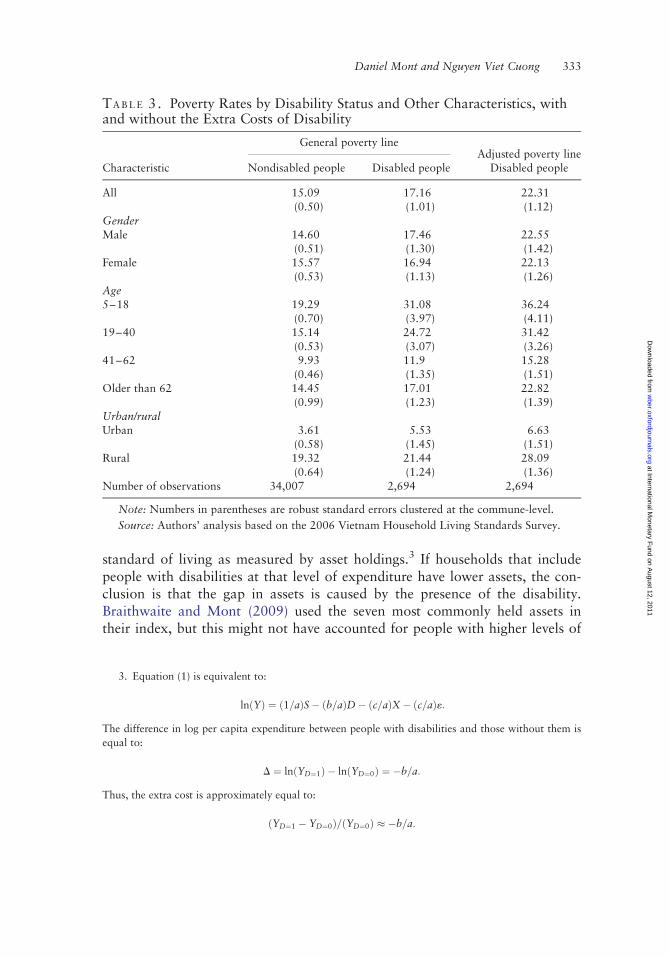
standard of living as measured by asset holdings.3 If households that includepeople with disabilities at that level of expenditure have lower assets, the con-clusion is that the gap in assets is caused by the presence of the disability.Braithwaite and Mont (2009) used the seven most commonly held assets intheir index, but this might not have accounted for people with higher levels of

TA B L E 3. Poverty Rates by Disability Status and Other Characteristics, withand without the Extra Costs of Disability

Characteristic

General poverty lineAdjusted poverty line

Nondisabled people Disabled people Disabled people

All 15.09 17.16 22.31(0.50) (1.01) (1.12)

GenderMale 14.60 17.46 22.55

(0.51) (1.30) (1.42)Female 15.57 16.94 22.13

(0.53) (1.13) (1.26)Age5–18 19.29 31.08 36.24

(0.70) (3.97) (4.11)19–40 15.14 24.72 31.42

(0.53) (3.07) (3.26)41–62 9.93 11.9 15.28

(0.46) (1.35) (1.51)Older than 62 14.45 17.01 22.82

(0.99) (1.23) (1.39)Urban/ruralUrban 3.61 5.53 6.63

(0.58) (1.45) (1.51)Rural 19.32 21.44 28.09

(0.64) (1.24) (1.36)Number of observations 34,007 2,694 2,694

Note: Numbers in parentheses are robust standard errors clustered at the commune-level.


3. Equation (1) is equivalent to:

lnðYÞ ¼ 1=að ÞS� b=að ÞD� c=að ÞX� c=að Þ1:

The difference in log per capita expenditure between people with disabilities and those without them is

equal to:

D ¼ lnðYD¼1Þ � lnðYD¼0Þ ¼ �b=a:

Thus, the extra cost is approximately equal to:

YD¼1 � YD¼0ð Þ= YD¼0ð Þ � �b=a:





Dow

nloaded from

wealth who were able to purchase other assets. Therefore, the asset list wasexpanded.4 The extra costs of disability were estimated to be 11.5 percent,slightly higher but of similar magnitude to the just over 9 percent inBraithwaite and Mont.5

There can be a problem of endogeneity of explanatory variables in equation (1).Thus, rather than estimate the causal effect of the explanatory variables in equation(1), the estimates are used to examine the difference in expenditures between peoplewith and without disabilities once asset holdings and other observed variables arecontrolled for.

Table 3 compares poverty rates for people with and without disabilities byvarious characteristics, both with an unadjusted poverty line and with apoverty line adjusted for the extra costs of disability. Since many householdsthat include a person with a disability are close to the poverty line, the povertyrates increase significantly when the poverty line is adjusted for the 11.5percent extra costs of disability, especially in rural areas.

Another striking finding is the much higher rate of poverty for householdsthat include a child or a prime age adult with disabilities (even withoutaccounting for the extra costs of disability). Of course, the causality may goboth ways. For example, poverty may lead to disability in children because ofthe lack of health care and proper nutrition. It may also lead to disability inadults, but it also probably limits their ability to generate a livelihood. Thedifference between the poverty rates for households without disabilities andthose with elderly disabled members is not that high, which brings up anotherpoint: when examining the relation between disability and poverty, it is impor-tant to account not only for the severity of the disability but also for the agewhen it was acquired. A child with a disability might be denied access to edu-cation and training and might experience a lifetime of discrimination. An adultwho acquires a disability might already have amassed certain skills and assets.And an elderly person who acquires a disability might be beyond working age,so although their families may incur certain costs in caring for them—includingforegone labor income—their own earnings potential might not be relevant.

Regression Analysis

The three regressions reported in table 4 therefore account not only for theseverity of disability (with separate regressions for DISLOW and DISHIGH)but also the age of onset of the disability—in particular, whether the disabilitybegan in childhood or adulthood. (The tables in this section present only theestimates of variables of interest such as DISLOW and DISHIGH. Fullregression results are in the appendix.)

4. The assets included in this analysis are motorbike; wardrobe; bed; tables, chairs, and sofas;

television; electric fan;. cooker; flush toilet; permanent house; and tapwater. The variable Y is per capita

expenditure, D is DISLOW, and X is a vector of household characteristics.

5. The estimate of - b / a is 0.115 (0.2281/1.9768), with a standard error of 0.026. The regression

of the asset index is in table A.3 in the appendix.





Dow

nloaded from

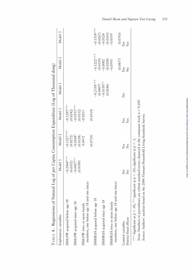
TA

BL

E4

.R

egre

ssio

ns

of

Nat

ura

lL

og

of

per

Capit

aC

onsu

mpti

on

Expen

dit

ure

(Log

of

Thousa

nd

dong)

Expla

nat

ory

vari

able

sM

odel

1M

odel

2M

odel

3M

odel

1M

odel

2M

odel

3

DIS

LO

Wac

quir

edbef

ore

age

18

–0.2

468***

–0.1

327***

–0.1

285***

(0.0

352)

(0.0

272)

(0.0

242)

DIS

LO

Wac

quir

edsi

nce

age

18

–0.0

427**

–0.0

268*

–0.0

353***

(0.0

189)

(0.0

158)

(0.0

132)

DIS

LO

W(t

wo

or

more

fam

ily

mem

ber

s,one

bef

ore

age

18

and

one

since

)0.0

472

–0.0

213

(0.0

710)

(0.0

519)

DIS

HIG

Hac

quir

edbef

ore

age

18

–0.2

358***

–0.1

222***

–0.1

314***

(0.0

407)

(0.0

319)

(0.0

267)

DIS

HIG

Hac

quir

edsi

nce

age

18

–0.0

530**

–0.0

082

–0.0

124

(0.0

246)

(0.0

208)

(0.0

165)

DIS

HIG

H(t

wo

or

more

fam

ily

mem

ber

s,one

bef

ore

age

18

and

one

since

)–

0.0

593

–0.0

559

(0.0

857)

(0.0

783)

Contr

ol

vari

able

sN

oY

esY

esN

oY

esY

esD

istr

ict

fixed

effe

cts

No

No

Yes

No

Yes

***

Sig

nifi

cant

atp

,.0

1;

**

signifi

cant

atp

,.0

5;

signifi

cant

atp

,.1

.

Note

:N

um

ber

sin

pare

nth

eses

are

robust

standard

erro

rscl

ust

ered

atth

eco

mm

une

leve

l;n¼

9,1

89.

Sourc

e:A

uth

ors

’analy

sis

base

don

the

2006

Vie

tnam

House

hold

Liv

ing

Sta

ndard

sSurv

ey.





Dow

nloaded from

Model 1 includes only disability variables (no control variables). Model 2includes several control variables. Model 3 includes district fixed-effects estima-tors,6 which help remove district variables that can affect both disability andhousehold welfare, such as epidemics and calamities.

The regressions show that households that include people with disabilitiesare more likely to be poor, regardless of the threshold of disability or when thedisability was acquired. However, the impact of the age of onset of disability isstriking. The relationship is much stronger and remains statistically significantafter controlling for a host of household characteristics.

Disability variables could have endogeneity problems; for example, house-holds might have experienced shocks that made their members more likely toacquire a disability and that also lowered income and consumption. Toexamine this issue, regressions included disability variables with more clearlyexogenous causes (war, accident, natural calamity, and birth defects) drawnfrom the survey question on the cause of the disability. For regressions of percapita expenditure (table A.5 in the appendix) and other the outcome variablesof employment and education, these disability variables have similar effects tothe overall disability variables (and thus are not reported here).

The age of onset also matters in the probability that a person with a disabil-ity is employed. With DISLOW, the negative impacts of having a disability arestrongly significant but are somewhat mitigated if that disability was acquiredas an adult (table 5). The same cannot be said of people considered to have adisability only when the more severe DISHIGH threshold is used: regardless ofage of onset, a disability reduces the probability of a person working by aboutthe same amount. These results hold whether looking at wage employment orhousehold employment for people ages 16–60.

These regressions also show that completion of primary schooling is associ-ated with a greater likelihood of working for the household business, whereascompleting secondary school tends to lead more often to wage work.

After controlling for education, the results show that people with disabilitieswork less and that their disability is associated with less education to beginwith. Enrollment rates are significantly lower for children with disabilities thanfor children without disabilities. For example, primary school enrollment forchildren ages 6–12 is nearly 96 percent for children without disabilities, butabout 69 percent for children with mild, moderate, or severe disabilities. Thegap is even higher when the more restrictive threshold is used. Given the impor-tance of education to livelihoods, this puts children with disabilities, on average,at a livelihood disadvantage from the beginning. The same result is found indeveloped countries (Loprest and Maag 2007).

6. A log function of per capita expenditure is used because expenditure follows a log normal

distribution rather than a normal distribution. Household characteristics that affect household earning

include household composition, human assets, physical assets, and regional and commune

characteristics (Glewwe 1991).





Dow

nloaded from

TA

BL

E5

.L

ogit

Reg

ress

ions

of

Em

plo

ym

ent

by

Deg

ree

of

Dis

abilit

yfo

rPeo

ple

Ages

16

–60

(Odds

Rat

ios)

Dep

enden

tvari

able

(1if

yes;

0,

oth

erw

ise)

Expla

nat

ory

vari

able

sW

ork

edfo

ra

wage

or

sala

ryW

ork

edfo

rth

ehouse

hold

Had

done

any

work

Work

edfo

ra

wage

or

sala

ryW

ork

edfo

rth

ehouse

hold

Had

done

any

work

DIS

LO

W0.3

155***

0.2

618***

0.0

498***

(0.0

648)

(0.0

399)

(0.0

083)

DIS

LO

Wfr

om

age

18

1.3

364

2.1

272***

3.0

159***

(0.3

234)

(0.3

740)

(0.5

769)

DIS

HIG

H0.2

574***

0.2

258***

0.0

390***

(0.0

624)

(0.0

396)

(0.0

073)

DIS

HIG

Hfr

om

age

18

0.9

081

1.3

102

1.4

810*

(0.3

020)

(0.2

909)

(0.3

427)

Contr

ol

vari

able

sY

esY

esY

esY

esY

esY

esD

istr

ict

fixed

effe

cts

Yes

Yes

Yes

Yes

Yes

Yes

***

Sig

nifi

cant

atp

,.0

1;

**

signifi

cant

atp

,.0

5;

signifi

cant

atp

,.1

.

Note

:N

um

ber

sin

pare

nth

eses

are

robust

standard

erro

rscl

ust

ered

atth

eco

mm

une

leve

l;n¼

24,7

10.

For

the

odds

rati

os

inth

elo

git

regre

ssio

ns,

‘sig

-nifi

cant’

mea

ns

‘sta

tist

icall

ydif

fere

nt’

from

one.

Sourc

e:A

uth

ors

’analy

sis

base

don

the

2006

Vie

tnam

House

hold

Liv

ing

Sta

ndard

sSurv

ey.





Dow

nloaded from

TA

BL

E6

.L

ogit

Reg

ress

ions

of

Educa

tion

(Odds

Rat

ios)

Expla

nat

ory

vari

able

Model

1M

odel

2M

odel

3M

odel

1M

odel

2M

odel

3

Dep

enden

tva

riab

leis

school

enro

llm

ent,

ages

6–

17

DIS

LO

W0.1

571***

0.0

842***

0.0

775***

(0.0

292)

(0.0

206)

(0.0

189)

DIS

HIG

H0.1

179***

0.0

682***

0.0

586***

(0.0

270)

(0.0

200)

(0.0

173)

Contr

ol

vari

able

sN

oY

esY

esN

oY

esY

esD

istr

ict

fixed

effe

cts

No

No

Yes

No

No

Yes

Dep

enden

tva

riab

leis

pri

mar

ysc

hool

com

ple

tion,

ages

18

–62

DIS

LO

Wby

aged

10

0.0

631***

0.0

269***

0.0

138***

(0.0

117)

(0.0

075)

(0.0

033)

DIS

HIG

Hby

aged

10

0.0

560***

0.0

223***

0.0

103***

(0.0

116)

(0.0

070)

(0.0

028)

Contr

ol

vari

able

sN

oY

esY

esN

oY

esY

esD

istr

ict

fixed

effe

cts

No

No

Yes

No

No

Yes

Dep

enden

tva

riab

leis

seco

ndar

ysc

hool

com

ple

tion,

ages

18

–62

DIS

LO

Wby

age

17

0.1

520***

0.1

185***

0.1

161***

(0.0

426)

(0.0

389)

(0.0

332)

DIS

HIG

Hby

age

17

0.1

812***

0.1

488***

0.1

372***

(0.0

536)

(0.0

500)

(0.0

424)

Contr

ol

vari

able

sN

oY

esY

esN

oY

esY

esD

istr

ict

fixed

effe

cts

No

No

Yes

No

No

Yes

***

Sig

nifi

cant

atp

,.0

1;

**

signifi

cant

atp

,.0

5;

signifi

cant

atp

,.1

.

Note

:N

um

ber

sin

pare

nth

eses

are

robust

standard

erro

rscl

ust

ered

atth

eco

mm

une

leve

l.E

nro

lled

insc

hool¼

1;

0,

oth

erw

ise.

Sourc

e:A

uth

ors

’es

tim

atio

nbase

don

the

2006

Vie

tnam

House

hold

Liv

ing

Sta

ndard

sSurv

ey.





Dow

nloaded from

A series of logit regressions were estimated to explore the relation betweendisability and education in Vietnam. Table 6 presents the estimates for the dis-ability variable coefficients; the full regressions are in tables A.8–A.10 in theappendix. For both DISLOW and DISHIGH, the correlation between disabil-ity and enrollment among school-age children is statistically significant at the 1percent significance level and increases as more explanatory variables areadded to the model. The odds ratios for the effect of disability on enrollmentusing the most inclusive specification (model 2) is 0.084, which for DISLOWtranslates into children with disabilities being nearly 0.41 times less likely toattend school, once other factors are controlled for. For DISHIGH, this risesto nearly 0.47 times.

In all specifications, having a disability in childhood significantly reduces thechances of completing school for older cohorts, regardless of the definition ofdisability or the type of school. The odds ratios using the most inclusive specifi-cation (model 2) from the school completion logits are 0.027 (primary) and0.119 (secondary) for DISLOW and 0.022 and 0.149 for DISHIGH. All aresignificant at 1 percent level.

These results show only that disability is associated with a lack of education;they do not explain the reasons behind the relationship. It could be thatparents want to send their children with disabilities to school but cannot,because of barriers such as transportation difficulties, lack of accessibleschools, and lack of training or acceptance by teachers. Or it could be thatparents do not want to send the children to school because the returns to edu-cation for children with disabilities do not warrant the investment, whether forreasons of inherent inability to benefit from schooling or of barriers to employ-ment (transportation, accessibility, attitudes, and so on) that prevent peoplewith disabilities from getting a return to the human capital they acquired inschool. In addition, poor parents might have limited resources for sending chil-dren to school and so may choose to spend them on their children with thehighest expected returns, perceiving their children without disabilities as beingthe better investment.

Whatever the case, the correlation between disability and education andemployment reveals that people with functional limitations have poorer out-comes than their peers without functional limitations.

I I I . C O N C L U S I O N

Disability, whether measured by a low or a high threshold, is significantly cor-related with poverty and lack of employment in Vietnam, using data from the2006 VHLSS. After accounting for the extra costs of disability, the correlationis stronger, especially in rural areas and for households with children andprime-age adults with disabilities. That correlation is also stronger for peoplewith more severe disabilities but is lower for people who acquire their





Dow

nloaded from

disabilities when they are adults. Disability during childhood is significantlycorrelated with lack of educational attainment, an important determinant ofpoverty.

Because of the endogeneity of this system—disability causing poverty,poverty causing disability, lack of returns in the labor market affectingschooling decisions, barriers to education affecting employment opportu-nities—it is difficult to attribute causality. It is clear, however, that peoplewith disabilities face more difficult and limited conditions and that thelimited conditions are highly significant when the extra costs of living witha disability are taken into account. For households with people with disabil-ities, ignoring the extra costs of disability means that poverty statistics canmiss these households whose standard of living, if the higher costs weretaken into account, would be equal to that of poor households withoutpeople with disabilities .

Better data on disability need to be collected in conjunction with data onconsumption and other measures of well-being. A clearer understanding of therelationship between disability and poverty and the barriers that disabledpeople face in fully participating in economic life will help policymakers deter-mine where the link between disability and poverty is strongest and where themost promising and appropriate avenues are for designing interventions toweaken that link.

REFERENCES

Altman, B.M. 2001. “Disability Definitions, Models, Classification Schemes, and Applications.” In

Handbook of Disability Studies, ed. G.L. Albrecht, K.D. Seelman, and M. Bury, 97–122. Thousand

Oaks, CA: Sage Publications.

Braithwaite, J., and D. Mont. 2009. “Disability and Poverty: A Survey of World Bank Poverty

Assessments and Implications.” Alter: European Journal of Disability Research 3: 219–32

CDC (Centers for Disease Control and Prevention). (2011). “Washington Group on Disability

Statistics,” www.cdc.gov/nchs/washington_group.htm.

Elwan, A. 1999. “Poverty and Disability: A Survey of the Literature.” SP Discussion Paper 9932, World

Bank, Washington, DC.

Fujii, T. 2008. “Two-Sample Estimation of Poverty Rates for Disabled People: An Application to

Tanzania.” Economics and Statistics Working Paper 02-2008, Singapore Management University,

Singapore.

Filmer, D. 2008. “Disability, Poverty, and Schooling in Developing Countries: Results from 11

Household Surveys.” The World Bank Economic Review 22 (1):141–63.

Gertler, P., and J. Gruber. 2002. “Insuring Consumption against Illness.” The American Economic

Review 92 (1): 51–70.

Glewwe, P. 1991. “Investigating the Determinants of Household Welfare in Cote d’Ivoire.” Journal of

Development Economics 35: 307–37.

Hoogeveen, J. 2005. “Measuring Welfare for Small but Vulnerable Groups: Poverty and Disability in

Uganda.” Journal of African Economies 14 (4): 603–31.

Kuklys, W. 2005. Amartya Sen’s Capability Approach: Theoretical Insights and Empirical Applications.

Studies in Choice and Welfare. New York: Springer-Verlag.

Loeb, M.E., A.H. Eide, and D. Mont. 2008. “Approaching the Measurement of Disability Prevalence:

The Case of Zambia.” Alter: European Journal of Disability Research 2 (1): 32–43.





Dow

nloaded from

Loeb, M.E., and D. Mont. 2010. “A Functional Approach to Assessing Health Impacts on People with

Disabilities.” Alter: European Journal of Disability Research 4 (3): 159–73.

Loprest, P., and E. Maag, 2007. “The Relationship between Early Disability Onset and Education and

Employment.” Journal of Vocational Rehabilitation 26 (1): 49–62.

C. Mete, ed. 2008. Economic Implications of Chronic Illness and Disease in Eastern Europe and the

Former Soviet Union. Washington, DC: The World Bank.

Miller, K., D. Mont, J. Madans, B. Altman, and A. Maitland 2010. “Results of a Cross-National

Structured Cognitive Interviewing Protocol to Test Measures of Disability.” Quantity and Quality.

45 (4): 801–815.

Mont, D. 2007a. “Measuring Disability Prevalence.” SP Discussion Paper 0706. World Bank,

Washington, DC.

———. 2007b. “Measuring Health and Disability.” The Lancet 369: 1658–63.

Mont, D., and M. Loeb. 2008. “Beyond DALYs: Developing Indicators to Assess the Impact of Public

Health Interventions on the Lives of People with Disabilities.” SP Discussion Paper 0815. World

Bank, Washington, DC.

Scott, K., and C. Mete. 2008. “Measurement of Disability and Linkages with Welfare, Employment,

and Schooling: The Case of Uzbekistan.” In Economic Implications of Chronic Illness and Disease

in Eastern Europe and the Former Soviet Union, ed. C. Mete. Washington, DC: World Bank.

Sen, A. 1985. Commodities and Capabilities. Amsterdam: North Holland.

———. 1993. “Capability and Well-being.” In The Quality of Life, ed. M. Nussbaum, and A.K. Sen.

Oxford: Clarendon Press.

———. 1999. Development as Freedom. Oxford: Oxford University Press.

Shakespeare, T., and N. Watson. 1997. “Defending the Social Model.” Disability and Society 12 (2):

293–300.

Tibble, M. 2005. “Review of the Existing Research on the Extra Costs of Disability.” Working Paper

21. Department for Work and Pensions, Leeds, UK.

Washington Group. 2008, “The Measurement of Disability: Recommendations for the 2010 Round of

Censuses.”Position paper available on www.cdc.gov/nchs/washington_group.htm.

WHO (World Health Organization). 2011. “International Classification of Functioning, Disability and

Health (ICF).” World Health Organization, http://www.who.int/classifications/icf/en/.

Yeo, R., and K. Moore. 2003. “Including Disabled People in Poverty Reduction Work: Nothing about

Us, without Us.” World Development 31 (3): 571–90

Zaidi, A., and T. Burchardt. 2005. “Comparing Incomes When Needs Differ: Equivalization for the

Extra Costs of Disability in the U.K.” Review of Income and Wealth 51 (1): 89–114.





Dow

nloaded from

A P P E N D I X

TA B L E A1. Correlation Coefficients of Functional Limitations for the Poorand Nonpoor

Functionallimitation Seeing Hearing

Rememberingand

concentrating Walking Self-care Communicating

PoorSeeing 1Hearing 0.432*** 1Remembering

andconcentrating

0.381*** 0.413*** 1

Walking 0.523*** 0.410*** 0.459*** 1Self-care 0.204*** 0.250*** 0.363*** 0.422*** 1Communicating 0.265*** 0.332*** 0.665*** 0.415*** 0.463*** 1NonpoorSeeing 1Hearing 0.348*** 1Remembering

andconcentrating

0.363*** 0.448*** 1

Walking 0.401*** 0.393*** 0.487*** 1Self-care 0.198*** 0.287*** 0.377*** 0.400*** 1Communicating 0.227*** 0.405*** 0.605*** 0.387*** 0.513*** 1

*** Significant at p , .01; ** significant at p , .05; significant at p , .1.


TA B L E A2. Relation between People with DISLOW and DISHIGH andHousehold Head

Age of disabled Head Head’s spouse Head’s children Head’s parent Others

DISLOWBefore age 18 0.00 0.00 85.63 0.00 14.37

(0.00) (0.00) (2.83) (0.00) (2.83)18–30 4.00 1.56 90.33 0.00 4.12

(1.68) (0.91) (2.56) (0.00) (1.80)31–40 30.61 13.56 41.82 0.00 14.01

(4.38) (3.27) (5.06) (0.00) (3.93)41–50 53.05 30.34 8.84 0.76 7.01

(3.10) (2.91) (2.17) (0.54) (1.73)Older than age 50 51.09 22.08 0.47 23.53 2.83

(1.04) (0.88) (0.17) (1.11) (0.42)Total 44.69 20.05 13.19 17.57 4.50

(0.89) (0.75) (0.71) (0.84) (0.46)DISHIGHBefore age 18 0.00 0.00 84.9 0.00 15.1

(0.00) (0.00) (3.63) (0.00) (3.63)18–30 3.31 0.49 91.96 0.00 4.25

(Continued)





Dow

nloaded from

TABLE A2. Continued

Age of disabled Head Head’s spouse Head’s children Head’s parent Others

(1.71) (0.49) (2.68) (0.00) (2.07)31–40 23.49 10.39 50.69 0.00 15.43

(4.91) (3.67) (6.38) (0.00) (5.07)41–50 49.91 17.13 16.45 0.89 15.63

(5.16) (3.71) (4.59) (0.88) (3.79)Older than age 50 44.9 18.73 0.95 31.3 4.12

(1.66) (1.35) (0.38) (1.70) (0.69)Total 36.33 14.8 20.9 21.22 6.75

(1.33) (1.02) (1.23) (1.23) (0.77)

*** Significant at p , .01; ** significant at p , .05; significant at p , .1.

Note: Number in parentheses are robust standard errors clustered at the commune level.DISLOW is the lower of two thresholds for determining when having difficulty performing activi-ties becomes a disability; DISHIGH, the higher threshold, excludes people with lesser difficulties.DISLOW and DISHIGH (see box 1).


TA B L E A3. Regression of Asset Index

Explanatory variable Coefficient Standard error p . t

Log of per capita expenditure 1.9768 0.0512 0.0000DISLOW –0.2281 0.0508 0.0000Ratio of children (before age 15) –0.3940 0.1096 0.0000Ratio of elderly (after age 60) –0.3389 0.0898 0.0000Household size 0.2366 0.0163 0.0000constant –9.8166 0.4585 0.0000R-squared 0.345Number of observations 9,189

Note: DISLOW is the lower of two thresholds for determining when having difficulty per-forming activities becomes a disability (see box 1).






Dow

nloaded from

TA

BL

EA

4.

Reg

ress

ions

of

Nat

ura

lL

ogari

thm

of

Per

Capit

aC

onsu

mpti

on

Expen

dit

ure

(Log

of

Thousa

nds

of

Dong)

Expla

nat

ory

vari

able

Model

1:

ord

inary

least

square

sM

odel

2:

ord

inary

least

square

sM

odel

3:

dis

tric

tfixed

effe

cts

Model

1:

ord

inary

least

square

sM

odel

2:

ord

inary

least

square

sM

odel

3:

dis

tric

tfixed

effe

cts

DIS

LO

WB

efore

age

18

–0.2

468***

–0.1

327***

–0.1

285***

(0.0

352)

(0.0

272)

(0.0

242)

18

and

old

er–

0.0

427**

–0.0

268*

–0.0

353***

(0.0

189)

(0.0

158)

(0.0

132)

Tw

oor

more

fam

ily

mem

ber

s,one

bef

ore

age

18

and

one

18

or

old

er

0.0

472

–0.0

213

(0.0

710)

(0.0

519)

DIS

HIG

HB

efore

age

18

–0.2

358***

–0.1

222***

–0.1

314***

(0.0

407)

(0.0

319)

(0.0

267)

18

and

old

er–

0.0

530**

–0.0

082

–0.0

124

(0.0

246)

(0.0

208)

(0.0

165)

Tw

oor

more

fam

ily

mem

ber

s,one

bef

ore

age

18

and

18

or

old

er

–0.0

593

–0.0

559

(0.0

857)

(0.0

783)

Urb

an

(yes¼

1)

0.3

941***

0.1

946***

0.3

943***

0.1

955***

(0.0

158)

(0.0

150)

(0.0

158)

(0.0

150)

House

hold

inR

edR

iver

Del

taO

mit

ted

House

hold

inN

ort

hE

ast

–0.1

444***

–0.1

464***

(0.0

193)

(0.0

193)

House

hold

inN

ort

hW

est

–0.2

886***

–0.2

894***

(0.0

329)

(0.0

329)

House

hold

inN

ort

hC

entr

al

Coast

–0.2

272***

–0.2

276***

(0.0

204)

(0.0

204)

House

hold

inSouth

Cen

tral

Coast

0.0

151

0.0

16





Dow

nloaded from

(0.0

209)

(0.0

208)

House

hold

inC

entr

al

Hig

hla

nds

–0.0

3–

0.0

323

(0.0

324)

(0.0

325)

House

hold

inSouth

East

0.3

243***

0.3

230***

(0.0

224)

(0.0

224)

House

hold

inM

ekong

Riv

erD

elta

0.1

677***

0.1

678***

(0.0

188)

(0.0

188)

Hea

dage

0.0

105***

0.0

067***

0.0

107***

0.0

071***

(0.0

032)

(0.0

025)

(0.0

032)

(0.0

025)

Hea

dage

square

d*

1,0

00

–0.0

707**

–0.0

439*

–0.0

741**

–0.0

489**

(0.0

304)

(0.0

237)

(0.0

306)

(0.0

237)

Hea

dw

ithout

educa

tion

deg

ree

Om

itte

d

Hea

dw

ith

pri

mary

school

deg

ree

0.1

740***

0.1

637***

0.1

738***

0.1

638***

(0.0

161)

(0.0

131)

(0.0

161)

(0.0

131)

Hea

dw

ith

low

erse

condary

school

0.2

953***

0.2

897***

0.2

961***

0.2

910***

(0.0

174)

(0.0

143)

(0.0

174)

(0.0

143)

Hea

dw

ith

upper

seco

ndary

school

0.4

799***

0.4

235***

0.4

810***

0.4

246***

(0.0

249)

(0.0

202)

(0.0

249)

(0.0

203)

Hea

dw

ith

tech

nic

al

deg

ree

0.5

657***

0.5

206***

0.5

667***

0.5

223***

(0.0

218)

(0.0

182)

(0.0

218)

(0.0

182)

Hea

dw

ith

post

–se

condary

school

0.8

632***

0.7

713***

0.8

652***

0.7

739***

(0.0

295)

(0.0

247)

(0.0

294)

(0.0

247)

Rat

ioof

childre

n(b

efore

age

15)

–0.5

144***

–0.5

352***

–0.5

124***

–0.5

311***

(Conti

nued

)





Dow

nloaded from

TA

BL

EA

4.

Conti

nued

Expla

nat

ory

vari

able

Model

1:

ord

inary

least

square

sM

odel

2:

ord

inary

least

square

sM

odel

3:

dis

tric

tfixed

effe

cts

Model

1:

ord

inary

least

square

sM

odel

2:

ord

inary

least

square

sM

odel

3:

dis

tric

tfixed

effe

cts

(0.0

329)

(0.0

282)

(0.0

331)

(0.0

282)

Rat

ioof

elder

ly(a

fter

age

60)

–0.2

150***

–0.2

082***

–0.2

241***

–0.2

202***

(0.0

331)

(0.0

267)

(0.0

325)

(0.0

265)

House

hold

size

–0.0

610***

–0.0

578***

–0.0

616***

–0.0

589***

(0.0

040)

(0.0

032)

(0.0

040)

(0.0

032)

Const

ant

8.5

406***

8.1

967***

8.3

724***

8.5

339***

8.1

894***

8.3

625***

(0.0

082)

(0.0

845)

(0.0

665)

(0.0

076)

(0.0

849)

(0.0

667)

R-s

quare

d0.0

10.4

80.3

00.0

10.4

80.3

0N

um

ber

of

obse

rvat

ions

9,1

89

***

Sig

nifi

cant

atp

,.0

1;

**

signifi

cant

atp

,.0

5;

signifi

cant

atp

,.1

.

Note

:N

um

ber

sin

pare

nth

eses

are

robust

standard

erro

rscl

ust

ered

atth

eco

mm

une

leve

l.D

ISL

OW

isth

elo

wer

of

two

thre

shold

sfo

rdet

erm

inin

gw

hen

hav

ing

dif

ficu

lty

per

form

ing

acti

vit

ies

bec

om

esa

dis

abilit

y;

DIS

HIG

H,

the

hig

her

thre

shold

,ex

cludes

peo

ple

wit

hle

sser

dif

ficu

ltie

s.D

ISL

OW

and

DIS

HIG

H(s

eebox

1).

Sourc

e:A

uth

ors

’analy

sis

base

don

the

2006

Vie

tnam

House

hold

Liv

ing

Sta

ndard

sSurv

ey.





Dow

nloaded from

TA

BL

EA

5.

Reg

ress

ions

of

Nat

ura

lL

ogari

thm

of

Per

Capit

aC

onsu

mpti

on

Expen

dit

ure

(Log

of

Thousa

nd

Dong):

Dis

abilit

ies

wit

hm

ore

Exogen

ous

Cause

s

Expla

nat

ory

vari

able

Model

1:

ord

inary

least

square

s

Model

2:

ord

inary

least

square

sM

odel

3:

dis

tric

tfixed

effe

cts

Model

1:

ord

inary

least

square

s

Model

2:

ord

inary

least

square

sM

odel

3:

dis

tric

tfixed

effe

cts

DIS

LO

WB

efore

age

18

–0.3

004***

–0.1

596***

–0.1

422***

(0.0

420)

(0.0

350)

(0.0

313)

Age

18

and

old

er–

0.0

291

–0.0

215

–0.0

316

(0.0

345)

(0.0

297)

(0.0

253)

Tw

oor

more

fam

ily

mem

ber

s,one

bef

ore

age

18

and

one

18

or

old

er)

0.0

207

–0.0

449

(0.0

958)

(0.0

678)

DIS

HIG

HB

efore

age

18

–0.3

060***

–0.1

537***

–0.1

452***

(0.0

479)

(0.0

410)

(0.0

332)

Age

18

or

old

er–

0.0

289

–0.0

004

–0.0

022

(0.0

439)

(0.0

382)

(0.0

309)

Tw

oor

more

fam

ily

mem

ber

s,one

bef

ore

age

18

and

one

18

or

old

er

–0.1

11

–0.1

745

(0.1

156)

(0.1

080)

Urb

an

(yes¼

1)

0.3

943***

0.1

962***

0.3

947***

0.1

967***

(0.0

158)

(0.0

150)

(0.0

158)

(0.0

150)

House

hold

inR

edR

iver

Del

taO

mit

ted

House

hold

inN

ort

hE

ast

–0.1

452***

–0.1

459***

(0.0

193)

(0.0

193)

House

hold

inN

ort

hW

est

–0.2

900***

–0.2

898***

(0.0

329)

(0.0

330)

(Conti

nued

)





Dow

nloaded from

TA

BL

EA

5.

Conti

nued

Expla

nat

ory

vari

able

Model

1:

ord

inary

least

square

s

Model

2:

ord

inary

least

square

sM

odel

3:

dis

tric

tfixed

effe

cts

Model

1:

ord

inary

least

square

s

Model

2:

ord

inary

least

square

sM

odel

3:

dis

tric

tfixed

effe

cts

House

hold

inN

ort

hC

entr

al

Coast

–0.2

267***

–0.2

273***

(0.0

204)

(0.0

204)

House

hold

inSouth

Cen

tral

Coast

0.0

153

0.0

156

(0.0

209)

(0.0

209)

House

hold

inC

entr

al

Hig

hla

nds

–0.0

322

–0.0

338

(0.0

323)

(0.0

325)

House

hold

inSouth

East

0.3

221***

0.3

219***

(0.0

224)

(0.0

224)

House

hold

inM

ekong

Riv

erD

elta

0.1

673***

0.1

675***

(0.0

188)

(0.0

188)

Hea

dage

0.0

109***

0.0

074***

0.0

108***

0.0

072***

(0.0

032)

(0.0

025)

(0.0

032)

(0.0

025)

Hea

dage

square

d*

1000

–0.0

760**

–0.0

513**

–0.0

746**

–0.0

502**

(0.0

302)

(0.0

236)

(0.0

303)

(0.0

236)

Hea

dw

ithout

educa

tion

deg

ree

Om

itte

d

Hea

dw

ith

pri

mary

school

deg

ree

0.1

731***

0.1

636***

0.1

728***

0.1

633***

(0.0

161)

(0.0

131)

(0.0

162)

(0.0

131)

Hea

dw

ith

low

erse

condary

school

0.2

951***

0.2

904***

0.2

956***

0.2

910***

(0.0

174)

(0.0

143)

(0.0

174)

(0.0

143)

Hea

dw

ith

upper

seco

ndary

school

0.4

790***

0.4

226***

0.4

799***

0.4

236***





Dow

nloaded from

(0.0

249)

(0.0

203)

(0.0

249)

(0.0

203)

Hea

dw

ith

tech

nic

al

deg

ree

0.5

654***

0.5

210***

0.5

656***

0.5

216***

(0.0

218)

(0.0

182)

(0.0

218)

(0.0

182)

Hea

dw

ith

post

seco

ndary

school

0.8

642***

0.7

728***

0.8

644***

0.7

737***

(0.0

295)

(0.0

247)

(0.0

295)

(0.0

247)

Rat

ioof

childre

n(b

efore

age

15)

–0.5

114***

–0.5

313***

–0.5

120***

–0.5

305***

(0.0

329)

(0.0

281)

(0.0

329)

(0.0

282)

Rat

ioof

elder

ly(a

fter

age

60)

–0.2

242***

–0.2

196***

–0.2

263***

–0.2

229***

(0.0

322)

(0.0

263)

(0.0

322)

(0.0

263)

House

hold

size

–0.0

620***

–0.0

591***

–0.0

620***

–0.0

594***

(0.0

040)

(0.0

032)

(0.0

040)

(0.0

032)

Const

ant

8.5

302***

8.1

885***

8.3

583***

8.5

279***

8.1

908***

8.3

603***

(0.0

072)

(0.0

843)

(0.0

665)

(0.0

072)

(0.0

843)

(0.0

665)

R-s

quare

d0.0

10.4

80.3

00.0

10.4

80.3

0N

um

ber

of

obse

rvat

ion

9,1

89

***

Sig

nifi

cant

atp

,.0

1;

**

signifi

cant

atp

,.0

5;

signifi

cant

atp

,.1

.

Note

:N

um

ber

sin

pare

nth

eses

are

robust

standard

erro

rscl

ust

ered

atth

eco

mm

une

leve

l.D

ISL

OW

isth

elo

wer

of

two

thre

shold

sfo

rdet

erm

inin

gw

hen

hav

ing

dif

ficu

lty

per

form

ing

acti

vit

ies

bec

om

esa

dis

abilit

y;

DIS

HIG

H,

the

hig

her

thre

shold

,ex

cludes

peo

ple

wit

hle

sser

dif

ficu

ltie

s.D

ISL

OW

and

DIS

HIG

H(s

eebox

1).

Sourc

e:A

uth

ors

’analy

sis

base

don

the

2006

Vie

tnam

House

hold

Liv

ing

Sta

ndard

sSurv

ey.





Dow

nloaded from

TA

BL

EA

6.

Logit

Reg

ress

ions

of

Em

plo

ymen

tby

Deg

ree

of

Dis

abilit

yon

Peo

ple

ages

16

–60

(Odds

Rat

ios)

Expla

nat

ory

var

iable

Work

edfo

ra

wage

or

sala

ryW

ork

edfo

rth

ehouse

hold

Had

done

any

work

Work

edfo

ra

wage

or

sala

ryW

ork

edfo

rth

ehouse

hold

Had

done

any

work

DIS

LO

W0.3

506***

0.2

985***

0.0

670***

(0.0

815)

(0.0

497)

(0.0

149)

DIS

LO

Wat

age

18

or

old

er1.2

843

1.9

983***

2.7

735***

(0.3

460)

(0.3

647)

(0.7

000)

DIS

HIG

H0.2

939***

0.2

554***

0.0

514***

(0.0

834)

(0.0

512)

(0.0

134)

DIS

HIG

Hat

age

18

or

old

er0.8

359

1.1

853

1.1

520

(0.3

156)

(0.2

863)

(0.3

559)

Age

1.2

170***

1.2

483***

1.9

014***

1.2

216***

1.2

507***

1.9

271***

(0.0

120)

(0.0

107)

(0.0

259)

(0.0

121)

(0.0

108)

(0.0

260)

Age

square

d0.9

971***

0.9

977***

0.9

921***

0.9

970***

0.9

977***

0.9

918***

(0.0

001)

(0.0

001)

(0.0

002)

(0.0

001)

(0.0

001)

(0.0

002)

No

educa

tion

dip

lom

aO

mit

ted

Com

ple

tion

of

pri

mary

school

0.8

400***

1.2

230***

1.1

129

0.8

429***

1.2

215***

1.1

087

(0.0

483)

(0.0

620)

(0.0

937)

(0.0

482)

(0.0

619)

(0.0

936)

Com

ple

tion

of

seco

ndary

school

2.1

238***

0.3

404***

0.4

674***

2.1

400***

0.3

408***

0.4

701***

(0.1

366)

(0.0

203)

(0.0

412)

(0.1

372)

(0.0

203)

(0.0

414)

Sex

(mal

e¼

1;

fem

ale¼

0)

1.9

721***

0.6

736***

1.5

603***

1.9

840***

0.6

779***

1.6

090***

(0.0

601)

(0.0

205)

(0.0

646)

(0.0

607)

(0.0

207)

(0.0

671)

Urb

an

(yes¼

1)

1.6

867***

0.3

918***

0.4

540***

1.6

861***

0.3

909***

0.4

480***

(0.0

779)

(0.0

194)

(0.0

247)

(0.0

779)

(0.0

193)

(0.0

243)

House

hold

size

0.9

714**

1.0

558***

1.0

285*

0.9

720**

1.0

571***

1.0

330**

(0.0

133)

(0.0

131)

(0.0

159)

(0.0

133)

(0.0

132)

(0.0

158)

House

hold

inR

edR

iver

Del

taO

mit

ted





Dow

nloaded from

House

hold

inN

ort

hE

ast

0.5

020***

2.3

173***

1.4

348***

0.4

975***

2.3

023***

1.4

083***

(0.0

345)

(0.1

617)

(0.1

125)

(0.0

342)

(0.1

607)

(0.1

108)

House

hold

inN

ort

hW

est

0.3

307***

3.5

289***

1.8

697***

0.3

288***

3.5

075***

1.8

368***

(0.0

355)

(0.3

822)

(0.2

593)

(0.0

351)

(0.3

802)

(0.2

577)

House

hold

inN

ort

h

Cen

tral

Coast

0.5

257

1.5

660***

0.8

046**

0.5

255***

1.5

653***

0.8

103**

(0.0

398)

(0.1

121)

(0.0

690)

(0.0

398)

(0.1

121)

(0.0

690)

House

hold

inSouth

Cen

tral

Coast

0.9

735

0.9

370

0.8

653

0.9

739

0.9

386

0.8

791

(0.0

741)

(0.0

763)

(0.0

802)

(0.0

742)

(0.0

764)

(0.0

817)

House

hold

inC

entr

al

Hig

hla

nds

0.5

375***

2.0

206***

1.2

969**

0.5

331***

1.9

983***

1.2

589**

(0.0

549)

(0.2

081)

(0.1

454)

(0.0

544)

(0.2

054)

(0.1

396)

House

hold

inSouth

East

1.2

887***

0.6

487***

0.7

173***

1.2

825***

0.6

442***

0.7

016***

(0.0

902)

(0.0

479)

(0.0

580)

(0.0

894)

(0.0

476)

(0.0

563)

House

hold

inM

ekong

Riv

erD

elta

1.0

313

0.9

636

0.9

023

1.0

285

0.9

606

0.8

946

(0.0

651)

(0.0

589)

(0.0

660)

(0.0

647)

(0.0

589)

(0.0

650)

Num

ber

of

obse

rvat

ions

24,7

10

***

Sig

nifi

cant

atp

,.0

1;

**

signifi

cant

atp

,.0

5;

signifi

cant

atp

,.1

.

Note

:N

um

ber

sin

pare

nth

eses

are

robust

standard

erro

rscl

ust

ered

atth

eco

mm

une

leve

l.D

ISL

OW

isth

elo

wer

of

two

thre

shold

sfo

rdet

erm

inin

gw

hen

hav

ing

dif

ficu

lty

per

form

ing

acti

vit

ies

bec

om

esa

dis

abilit

y;

DIS

HIG

H,

the

hig

her

thre

shold

,ex

cludes

peo

ple

wit

hle

sser

dif

ficu

ltie

s.D

ISL

OW

and

DIS

HIG

H(s

eebox

1).

Sourc

e:A

uth

ors

’analy

sis

base

don

the

2006

Vie

tnam

House

hold

Liv

ing

Sta

ndard

sSurv

ey.





Dow

nloaded from

TA

BL

EA

7.

Dis

tric

tFix

edE

ffec

tsL

ogit

Reg

ress

ion

of

Em

plo

ymen

tby

Deg

ree

of

Dis

abilit

yon

Peo

ple

Ages

16

–60

(Odds

Rat

ios)

Expla

nat

ory

vari

able

Work

edfo

ra

wage

or

sala

ryW

ork

edfo

rth

ehouse

hold

Had

done

any

work

Work

edfo

ra

wage

or

sala

ryW

ork

edfo

rth

ehouse

hold

Had

done

any

work

DIS

LO

W0.3

155***

0.2

618***

0.0

498***

(0.0

648)

(0.0

399)

(0.0

083)

DIS

LO

Wat

age

18

or

old

er1.3

364

2.1

272***

3.0

159***

(0.3

234)

(0.3

740)

(0.5

769)

DIS

HIG

H0.2

574***

0.2

258***

0.0

390***

(0.0

624)

(0.0

396)

(0.0

073)

DIS

HIG

Hat

age

18

or

old

er0.9

081

1.3

102

1.4

810*

(0.3

020)

(0.2

909)

(0.3

427)

Age

1.2

273***

1.2

652***

1.9

576***

1.2

320***

1.2

673***

1.9

792***

(0.0

109)

(0.0

100)

(0.0

243)

(0.0

108)

(0.0

100)

(0.0

247)

Age

square

d0.9

970***

0.9

976***

0.9

917***

0.9

969***

0.9

975***

0.9

915***

(0.0

001)

(0.0

001)

(0.0

002)

(0.0

001)

(0.0

001)

(0.0

002)

No

educa

tion

dip

lom

aO

mit

ted





Dow

nloaded from

Com

ple

tion

of

pri

mary

school

0.8

129***

1.2

898***

1.1

420*

0.8

155***

1.2

892***

1.1

425*

(0.0

407)

(0.0

598)

(0.0

854)

(0.0

408)

(0.0

599)

(0.0

860)

Com

ple

tion

of

seco

ndary

school

1.9

437***

0.3

825***

0.4

851***

1.9

599***

0.3

839***

0.4

920***

(0.1

088)

(0.0

207)

(0.0

393)

(0.1

096)

(0.0

207)

(0.0

400)

Sex

(male¼

1;

fem

ale¼

0)

2.0

499***

0.6

483***

1.5

674***

2.0

620***

0.6

517***

1.6

032***

(0.0

654)

(0.0

200)

(0.0

676)

(0.0

658)

(0.0

201)

(0.0

694)

Urb

an

(yes¼

1)

1.4

263***

0.5

270***

0.5

532***

1.4

262***

0.5

270***

0.5

526***

(0.0

732)

(0.0

268)

(0.0

388)

(0.0

732)

(0.0

268)

(0.0

388)

House

hold

size

0.9

691***

1.0

447***

1.0

070

0.9

703***

1.0

464***

1.0

137

(0.0

103)

(0.0

104)

(0.0

139)

(0.0

103)

(0.0

105)

(0.0

140)

Num

ber

of

obse

rvat

ions

23,9

38

24,3

83

24,0

37

23,9

38

24,3

83

24,0

37

Num

ber

of

dis

tric

ts587

607

585

587

607

585

***

Sig

nifi

cant

atp

,.0

1;

**

signifi

cant

atp

,.0

5;

signifi

cant

atp

,.1

.

Note

:N

um

ber

sin

pare

nth

eses

are

robust

standard

erro

rscl

ust

ered

atth

eco

mm

une

leve

l.D

ISL

OW

isth

elo

wer

of

two

thre

shold

sfo

rdet

erm

inin

gw

hen

hav

ing

dif

ficu

lty

per

form

ing

acti

vit

ies

bec

om

esa

dis

abilit

y;

DIS

HIG

H,

the

hig

her

thre

shold

,ex

cludes

peo

ple

wit

hle

sser

dif

ficu

ltie

s.D

ISL

OW

and

DIS

HIG

H(s

eebox

1).

Sourc

e:A

uth

ors

’analy

sis

base

don

the

2006

Vie

tnam

House

hold

Liv

ing

Sta

ndard

sSurv

ey.





Dow

nloaded from

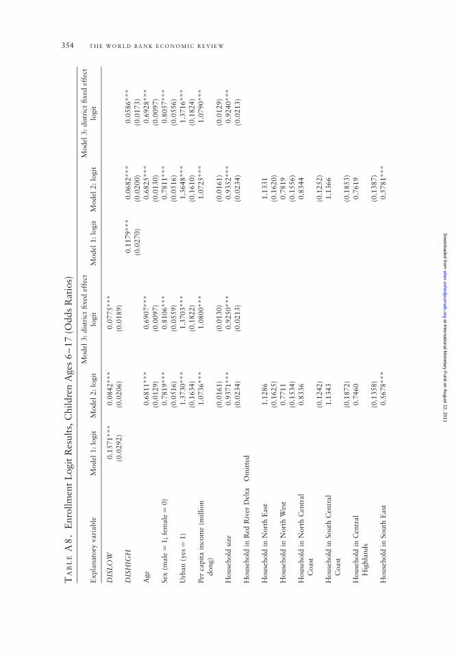
TA

BL

EA

8.

Enro

llm

ent

Logit

Res

ult

s,C

hil

dre

nA

ges

6–

17

(Odds

Rat

ios)

Expla

nat

ory

var

iable

Model

1:

logit

Model

2:

logit

Model

3:

dis

tric

tfixed

effe

ctlo

git

Model

1:

logit

Model

2:

logi

tM

odel

3:

dis

tric

tfixed

effe

ctlo

git

DIS

LO

W0.1

571***

0.0

842***

0.0

775***

(0.0

292)

(0.0

206)

(0.0

189)

DIS

HIG

H0.1

179***

0.0

682***

0.0

586***

(0.0

270)

(0.0

200)

(0.0

173)

Age

0.6

811***

0.6

907***

0.6

825***

0.6

928***

(0.0

129)

(0.0

097)

(0.0

130)

(0.0

097)

Sex

(mal

e¼

1;

fem

ale¼

0)

0.7

819***

0.8

106***

0.7

811***

0.8

057***

(0.0

516)

(0.0

559)

(0.0

516)

(0.0

556)

Urb

an

(yes¼

1)

1.3

730***

1.3

703***

1.3

648***

1.3

716***

(0.1

634)

(0.1

822)

(0.1

610)

(0.1

824)

Per

capit

ain

com

e(m

illion

dong)

1.0

736***

1.0

800***

1.0

725***

1.0

790***

(0.0

161)

(0.0

130)

(0.0

161)

(0.0

129)

House

hold

size

0.9

371***

0.9

250***

0.9

352***

0.9

240***

(0.0

234)

(0.0

213)

(0.0

234)

(0.0

213)

House

hold

inR

edR

iver

Del

taO

mit

ted

House

hold

inN

ort

hE

ast

1.1

286

1.1

331

(0.1

625)

(0.1

620)

House

hold

inN

ort

hW

est

0.7

711

0.7

819

(0.1

534)

(0.1

556)

House

hold

inN

ort

hC

entr

al

Coast

0.8

336

0.8

344

(0.1

242)

(0.1

252)

House

hold

inSouth

Cen

tral

Coast

1.1

343

1.1

366

(0.1

872)

(0.1

853)

House

hold

inC

entr

al

Hig

hla

nds

0.7

460

0.7

619

(0.1

358)

(0.1

387)

House

hold

inSouth

East

0.5

678***

0.5

781***





Dow

nloaded from

(0.0

903)

(0.0

919)

House

hold

inM

ekong

Riv

erD

elta

0.5

385***

0.5

466***

(0.0

716)

(0.0

727)

Hea

dw

ithout

educa

tion

deg

ree

Om

itte

d

Hea

dw

ith

pri

mar

ysc

hool

deg

ree

1.6

258***

1.6

487***

1.6

177***

1.6

356***

(0.1

463)

(0.1

500)

(0.1

456)

(0.1

488)

Hea

dw

ith

low

er–

seco

ndary

school

2.8

462***

2.7

594***

2.8

434***

2.7

927***

(0.3

102)

(0.3

118)

(0.3

099)

(0.3

156)

Hea

dw

ith

upper

seco

ndary

school

4.5

997***

4.0

878***

4.5

951***

4.0

552***

(0.8

923)

(0.8

216)

(0.8

915)

(0.8

151)

Hea

dw

ith

tech

nic

al

deg

ree

8.1

011***

7.6

141***

8.2

482***

7.8

381***

(2.2

764)

(1.7

817)

(2.3

425)

(1.8

420)

Hea

dw

ith

post

–se

condary

school

7.9

486***

8.8

110***

7.8

538***

8.8

640***

(3.5

292)

(4.0

266)

(3.5

421)

(4.0

509)

Num

ber

of

obse

rvat

ions

9,8

80

9,8

80

8,3

52

9,8

80

9,8

80

8,3

52

***

Sig

nifi

cant

atp

,.0

1;

**

signifi

cant

atp

,.0

5;

signifi

cant

atp

,.1

.

Note

:N

um

ber

sin

pare

nth

eses

are

robust

standard

erro

rscl

ust

ered

atth

eco

mm

une

leve

l.D

ISL

OW

isth

elo

wer

of

two

thre

shold

sfo

rdet

erm

inin

gw

hen

hav

ing

dif

ficu

lty

per

form

ing

acti

vit

ies

bec

om

esa

dis

abilit

y;

DIS

HIG

H,

the

hig

her

thre

shold

,ex

cludes

peo

ple

wit

hle

sser

dif

ficu

ltie

s.D

ISL

OW

and

DIS

HIG

H(s

eebox

1).

Sourc

e:A

uth

ors

’analy

sis

base

don

the

2006

Vie

tnam

House

hold

Liv

ing

Sta

ndard

sSurv

ey.





Dow

nloaded from

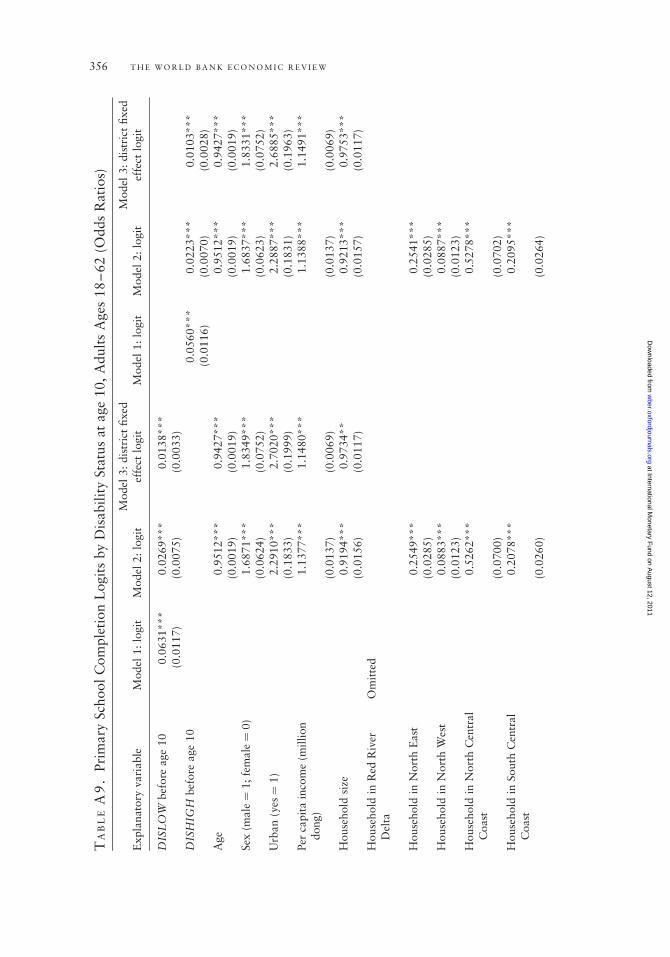
TA

BL

EA

9.

Pri

mary

Sch

ool

Com

ple

tion

Logit

sby

Dis

abilit

ySta

tus

atage

10,

Adult

sA

ges

18

–62

(Odds

Rat

ios)

Expla

nat

ory

vari

able

Model

1:

logit

Model

2:

logit

Model

3:

dis

tric

tfixed

effe

ctlo

git

Model

1:

logit

Model

2:

logit

Model

3:

dis

tric

tfixed

effe

ctlo

git

DIS

LO

Wbef

ore

age

10

0.0

631***

0.0

269***

0.0

138***

(0.0

117)

(0.0

075)

(0.0

033)

DIS

HIG

Hbef

ore

age

10

0.0

560***

0.0

223***

0.0

103***

(0.0

116)

(0.0

070)

(0.0

028)

Age

0.9

512***

0.9

427***

0.9

512***

0.9

427***

(0.0

019)

(0.0

019)

(0.0

019)

(0.0

019)

Sex

(male¼

1;

fem

ale¼

0)

1.6

871***

1.8

349***

1.6

837***

1.8

331***

(0.0

624)

(0.0

752)

(0.0

623)

(0.0

752)

Urb

an

(yes¼

1)

2.2

910***

2.7

020***

2.2

887***

2.6

885***

(0.1

833)

(0.1

999)

(0.1

831)

(0.1

963)

Per

capit

ain

com

e(m

illi

on

dong)

1.1

377***

1.1

480***

1.1

388***

1.1

491***

(0.0

137)

(0.0

069)

(0.0

137)

(0.0

069)

House

hold

size

0.9

194***

0.9

734**

0.9

213***

0.9

753***

(0.0

156)

(0.0

117)

(0.0

157)

(0.0

117)

House

hold

inR

edR

iver

Del

taO

mit

ted

House

hold

inN

ort

hE

ast

0.2

549***

0.2

541***

(0.0

285)

(0.0

285)

House

hold

inN

ort

hW

est

0.0

883***

0.0

887***

(0.0

123)

(0.0

123)

House

hold

inN

ort

hC

entr

al

Coast

0.5

262***

0.5

278***

(0.0

700)

(0.0

702)

House

hold

inSouth

Cen

tral

Coast

0.2

078***

0.2

095***

(0.0

260)

(0.0

264)





Dow

nloaded from

House

hold

inC

entr

al

Hig

hla

nds

0.1

116***

0.1

109***

(0.0

152)

(0.0

151)

House

hold

inSouth

East

0.1

143***

0.1

147***

(0.0

133)

(0.0

134)

House

hold

inM

ekong

Riv

erD

elta

0.0

669***

0.0

671***

(0.0

064)

(0.0

065)

Num

ber

of

obse

rvat

ions

23,0

12

23,0

12

21,3

68

23,0

12

23,0

12

21,3

68

***

Sig

nifi

cant

atp

,.0

1;

**

signifi

cant

atp

,.0

5;

signifi

cant

atp

,.1

.

Note

:N

um

ber

sin

pare

nth

eses

are

robust

standard

erro

rscl

ust

ered

atth

eco

mm

une

leve

l.

Sourc

e:A

uth

ors

’analy

sis

base

don

the

2006

Vie

tnam

House

hold

Liv

ing

Sta

ndard

sSurv

ey.





Dow

nloaded from

TA

BL

EA

10

.Sec

ondary

Sch

ool

Com

ple

tion

Logit

sby

Dis

abilit

ySta

tus,

Adult

sA

ges

18

–62

(Odds

Rat

ios)

Expla

nat

ory

vari

able

Model

1:

logit

Model

2:

logit

Model

3:

dis

tric

tfixed

effe

ctlo

git

Model

1:

logit

Model

2:

logit

Model

3:

dis

tric

tfixed

effe

ctlo

git

DIS

LO

Wbef

ore

age

17

0.1

520***

0.1

185***

0.1

161***

(0.0

426)

(0.0

389)

(0.0

332)

DIS

HIG

Hbef

ore

age

17

0.1

812***

0.1

488***

0.1

372***

(0.0

536)

(0.0

500)

(0.0

424)

Age

0.9

550***

0.9

522***

0.9

550***

0.9

531***

(0.0

019)

(0.0

019)

(0.0

019)

(0.0

019)

Sex

(male¼

1;

fem

ale¼

0)

1.4

492***

1.5

235***

1.4

477***

1.5

204***

(0.0

449)

(0.0

518)

(0.0

449)

(0.0

517)

Urb

an

(yes¼

1)

3.2

871***

3.1

740***

3.2

838***

3.1

772***

(0.1

972)

(0.1

746)

(0.1

970)

(0.1

747)

Per

capit

ain

com

e(m

illion

dong)

1.1

052***

1.1

041***

1.1

052***

1.1

041***

(0.0

077)

(0.0

033)

(0.0

077)

(0.0

033)

House

hold

size

0.9

380***

0.9

550***

0.9

389***

0.9

550***

(0.0

141)

(0.0

115)

(0.0

141)

(0.0

115)

House

hold

inR

edR

iver

Del

taO

mit

ted

House

hold

inN

ort

hE

ast

0.7

672***

0.7

664***

(0.0

598)

(0.0

598)

House

hold

inN

ort

hW

est

0.4

848***

0.4

853***

(0.0

664)

(0.0

665)

House

hold

inN

ort

hC

entr

al

Coast

0.8

033**

0.8

033**

(0.0

707)

(0.0

707)





Dow

nloaded from

House

hold

inSouth

Cen

tral

Coast

0.5

764***

0.5

781***

(0.0

530)

(0.0

532)

House

hold

inC

entr

al

Hig

hla

nds

0.4

185***

0.4

173***

(0.0

477)

(0.0

476)

House

hold

inSouth

East

0.3

910***

0.3

914***

(0.0

352)

(0.0

352)

House

hold

inM

ekong

Riv

erD

elta

0.2

161***

0.2

165***

(0.0

177)

(0.0

178)

Num

ber

of

obse

rvat

ions

23,0

12

23,0

12

22,2

47

23,0

12

23,0

12

22,2

47

***

Sig

nifi

cant

atp

,.0

1;

**

signifi

cant

atp

,.0

5;

signifi

cant

atp

,.1

.

Note

:N

um

ber

sin

pare

nth

eses

are

robust

standard

erro

rscl

ust

ered

atth

eco

mm

une

leve

l.

Sourc

e:A

uth

ors

’analy

sis

base

don

the

2006

Vie

tnam

House

hold

Liv

ing

Sta

ndard

sSurv

ey.





Dow

nloaded from


editorsAlain de Janvry and Elisabeth Sadoulet, University of California at Berkeley

assistant to the editor Marja Kuiper

editorial boardHarold H. Alderman, World Bank (retired)Pranab K. Bardhan, University of California,

BerkeleyScott Barrett, Columbia University, USAAsli Demirgüç-Kunt, World Bank Jean-Jacques Dethier, World BankQuy-Toan Do, World BankFrédéric Docquier, Catholic University of

Louvain, BelgiumEliana La Ferrara, Università Bocconi, ItalyFrancisco H. G. Ferreira, World BankAugustin Kwasi Fosu, United Nations

University, WIDER, FinlandPaul Glewwe, University of Minnesota,

USAAnn E. Harrison, World BankPhilip E. Keefer, World BankJustin Yifu Lin, World BankNorman V. Loayza, World Bank

William F. Maloney, World BankDavid J. McKenzie, World BankJaime de Melo, University of GenevaJuan-Pablo Nicolini, Universidad Torcuato di

Tella, ArgentinaNina Pavcnik, Dartmouth College, USAVijayendra Rao, World BankMartin Ravallion, World BankJaime Saavedra-Chanduvi, World BankClaudia Paz Sepúlveda, World BankJoseph Stiglitz, Columbia University, USAJonathan Temple, University of Bristol, UKRomain Wacziarg, University of California,

Los Angeles, USADominique Van De Walle, World BankChristopher M. Woodruff, University of

California, San DiegoYaohui Zhao, CCER, Peking University,

China

The World Bank Economic Review is a professional journal used for the dissemination of research indevelopment economics broadly relevant to the development profession and to the World Bank inpursuing its development mandate. It is directed to an international readership among economists andsocial scientists in government, business, international agencies, universities, and development researchinstitutions. The Review seeks to provide the most current and best research in the field of quantita-tive development policy analysis, emphasizing policy relevance and operational aspects of economics,rather than primarily theoretical and methodological issues. Consistency with World Bank policy playsno role in the selection of articles.

The Review is managed by one or two independent editors selected for their academic excellence inthe field of development economics and policy.The editors are assisted by an editorial board composedin equal parts of scholars internal and external to the World Bank. World Bank staff and outsideresearchers are equally invited to submit their research papers to the Review.

For more information, please visit the Web sites of the Economic Review at Oxford University Pressat www.wber.oxfordjournals.org and at the World Bank at www.worldbank.org/research/journals.

Instructions for authors wishing to submit articles are available online at www.wber.oxfordjournals.org.Please direct all editorial correspondence to the Editor at [email protected].

Forthcoming papers in

• What Constrains Africa’s Exports?Caroline Freund and Nadia Rocha

• Does the Internet Reduce Corruption? Evidence from U.S. States and across CountriesThomas Barnebeck Andersen, Jeanet Bentzen, Carl-Johan Dalgaard, andPablo Selaya

• Do Labor Statistics Depend on How and to Whom the Questions Are Asked? Results from a Survey Experiment in TanzaniaElena Bardasi, Kathleen Beegle, Andrew Dillon, and Pieter Serneels

• Entrepreneurship and Development: the Role of InformationAsymmetriesLeora Klapper and Inessa Love

• Getting Credit to High Return Microentrepreneurs: The Results of an Information InterventionSuresh de Mel, David McKenzie, and Christopher Woodruff

• The Impact of the Business Environment on Young Firm Financing Larry W. Chavis, Leora F. Klapper, and Inessa Love

• Does a Picture Paint a Thousand Words? Evidence from a Microcredit Marketing ExperimentXavier Giné, Ghazala Mansuri, and Mario Picón

• Entrepreneurship and the Extensive Margin in Export Growth:A Microeconomic Accounting of Costa Rica’s Export Growth during 1997-2007Daniel Lederman, Andrés Rodríguez-Clare, and Daniel Yi Xu


SYMPOSIUM ON ENTREPRENEURSHIP AND DEVELOPMENT


Has India’s Economic Growth Become More Pro-Poor in the Wake of Economic Reforms?


Are The Poverty Effects of Trade Policies Invisible?Monika Verma, Thomas W. Hertel, and Ernesto Valenzuela

Corruption and Confidence in Public Institutions: Evidence from a Global Survey


Agricultural Distortions in Sub-Saharan Africa: Trade and WelfareIndicators, 1961 to 2004


Thresholds in the Finance-Growth Nexus: A Cross-Country AnalysisHakan Yilmazkuday

The Value of Vocational Education: High School Type and LaborMarket Outcomes in Indonesia


Disability and Poverty in VietnamDaniel Mont and Nguyen Viet Cuong

Volume 25 • 2011 • Number 2

www.wber.oxfordjournals.org

THE WORLD BANK1818 H Street, NWWashington, DC 20433, USAWorld Wide Web: http://www.worldbank.org/E-mail: [email protected]

2V

olume 25 • N

umber 2 • 2011

TH

E W

OR

LD

BA

NK

EC

ON

OM

IC R

EV

IEW

Pages 157–359

ISSN 0258-6770 (PRINT) ISSN 1564-698X (ONLINE)

80517 - world bank documents

Documents