71 2013 hess estimating eta etp eto epan standard met data pragmatic synthesis

Hydrol. Earth Syst. Sci., 17, 1331–1363, 2013www.hydrol-earth-syst-sci.net/17/1331/2013/doi:10.5194/hess-17-1331-2013© Author(s) 2013. CC Attribution 3.0 License.

EGU Journal Logos (RGB)

Advances in Geosciences

Open A

ccess

Natural Hazards and Earth System

Sciences

Open A

ccess

Annales Geophysicae

Open A

ccess

Nonlinear Processes in Geophysics

Open A

ccess

Atmospheric Chemistry

and Physics

Open A

ccess

Atmospheric Chemistry

and Physics

Open A

ccess

Discussions

Atmospheric Measurement

Techniques

Open A

ccess

Atmospheric Measurement

Techniques

Open A

ccess

Discussions

Biogeosciences

Open A

ccess

Open A

ccess

BiogeosciencesDiscussions

Climate of the Past

Open A

ccess

Open A

ccess

Climate of the Past

Discussions

Earth System Dynamics

Open A

ccess

Open A

ccess

Earth System Dynamics

Discussions

GeoscientificInstrumentation

Methods andData Systems

Open A

ccess

GeoscientificInstrumentation

Methods andData Systems

Open A

ccess

Discussions

GeoscientificModel Development

Open A

ccess

Open A

ccess

GeoscientificModel Development

Discussions

Hydrology and Earth System

SciencesO

pen Access

Hydrology and Earth System

Sciences

Open A

ccess

Discussions

Ocean Science

Open A

ccess

Open A

ccess

Ocean ScienceDiscussions

Solid Earth

Open A

ccess

Open A

ccess

Solid EarthDiscussions

The Cryosphere

Open A

ccess

Open A

ccess

The CryosphereDiscussions

Natural Hazards and Earth System

Sciences

Open A

ccess

Discussions

Estimating actual, potential, reference crop and pan evaporationusing standard meteorological data: a pragmatic synthesis

T. A. McMahon1, M. C. Peel1, L. Lowe2, R. Srikanthan3, and T. R. McVicar4

1Department of Infrastructure Engineering, The University of Melbourne, Parkville, Victoria, 3010, Australia2Sinclair Knight Merz, P.O. Box 312, Flinders Lane, Melbourne, 8009, Australia3Water Division, Bureau of Meteorology, GPO 1289, Melbourne, 3001, Australia4Land and Water Division, Commonwealth Scientific and Industrial Research Organisation, Clunies Ross Drive,Acton, ACT 2602, Australia

Correspondence to:T. A. McMahon ([email protected])

Received: 19 September 2012 – Published in Hydrol. Earth Syst. Sci. Discuss.: 18 October 2012Revised: 26 February 2013 – Accepted: 14 March 2013 – Published: 10 April 2013

Abstract. This guide to estimating daily and monthly ac-tual, potential, reference crop and pan evaporation coverstopics that are of interest to researchers, consulting hydrol-ogists and practicing engineers. Topics include estimatingactual evaporation from deep lakes and from farm damsand for catchment water balance studies, estimating poten-tial evaporation as input to rainfall-runoff models, and refer-ence crop evapotranspiration for small irrigation areas, andfor irrigation within large irrigation districts. Inspiration forthis guide arose in response to the authors’ experiences inreviewing research papers and consulting reports where es-timation of the actual evaporation component in catchmentand water balance studies was often inadequately handled.Practical guides using consistent terminology that cover boththeory and practice are not readily available. Here we pro-vide such a guide, which is divided into three parts. The firstpart provides background theory and an outline of the con-ceptual models of potential evaporation of Penman, Penman–Monteith and Priestley–Taylor, as well as discussions of ref-erence crop evapotranspiration and Class-A pan evapora-tion. The last two sub-sections in this first part include tech-niques to estimate actual evaporation from (i) open-surfacewater and (ii) landscapes and catchments (Morton and theadvection-aridity models). The second part addresses topicsconfronting a practicing hydrologist, e.g. estimating actualevaporation for deep lakes, shallow lakes and farm dams,lakes covered with vegetation, catchments, irrigation areasand bare soil. The third part addresses six related issues:(i) automatic (hard wired) calculation of evaporation esti-

mates in commercial weather stations, (ii) evaporation esti-mates without wind data, (iii) at-site meteorological data, (iv)dealing with evaporation in a climate change environment,(v) 24 h versus day-light hour estimation of meteorologicalvariables, and (vi) uncertainty in evaporation estimates.

This paper is supported by a Supplement that includes 21sections enhancing the material in the text, worked examplesof many procedures discussed in the paper, a program list-ing (Fortran 90) of Morton’s WREVAP evaporation modelsalong with tables of monthly Class-A pan coefficients for 68locations across Australia and other information.

1 Introduction

Actual evaporation is a major component in the water bal-ance of a catchment, reservoir or lake, irrigation region, andsome groundwater systems. For example, across all conti-nents evapotranspiration is 70 % of precipitation, and variesfrom over 90 % in Australia to approximately 60 % in Europe(Baumgarter and Reichel, 1975, Table 12). For major reser-voirs in Australia, actual evaporation losses represent 20 %of reservoir yield (Hoy and Stephens, 1979, p. 1). Comparedwith precipitation and streamflow, the magnitude of actualevaporation over the long term is more difficult to estimatethan either precipitation or streamflow.

This paper deals with estimating actual, potential, refer-ence crop and pan evaporation at a daily and a monthly timestep using standard meteorological data. A major discussion

Published by Copernicus Publications on behalf of the European Geosciences Union.

1332 T. A. McMahon et al.: Estimating evaporation

of the use of remotely sensed data to estimate actual evapo-ration is outside the scope of this paper but readers interestedin the topic are referred to Kalma et al. (2008) and Glenn etal. (2010) for relevant material.

1.1 Background

The inspiration for the paper, which is a considered sum-mary of techniques rather than a review, arose because overrecent years the authors have reviewed many research pa-pers and consulting reports in which the estimation of theactual evaporation component in catchment and water bal-ance studies was inadequately handled. Our examination ofthe literature yielded few documents covering both theoryand practice that are readily available to a researcher, con-sulting hydrologist or practicing engineer. Chapter 7Evap-otranspiration in Physical Hydrologyby Dingman (1992),Chapter 4Evaporation(Shuttleworth, 1992) in theHand-book of Hydrology(Maidment, 1992) and, for irrigated areas,FAO 56 Crop evapotranspiration: Guidelines for computingcrop water requirements(Allen et al., 1998) are helpful ref-erences. We refer heavily to these texts in this paper whichis aimed at improving the practice of estimating actual andpotential evaporation, reference crop evapotranspiration andpan evaporation using standard daily or monthly meteoro-logical data. This paper is not intended to be an introductionto evaporation processes. Dingman (1992) provides such anintroduction. Readers, who wish to develop a strong theo-retical background of evaporation processes, are referred toEvaporation into the Atmosphereby Brutsaert (1982), and toShuttleworth (2007) for a historical perspective.

There are many practical situations where daily or monthlyactual or potential evaporation estimates are required. For ex-ample, for deep lakes or post-mining voids, shallow lakes orfarm dams, catchment water balance studies (in which ac-tual evaporation may be land-cover specific or lumped de-pending on the style of analysis or modelling), rainfall-runoffmodelling, or small irrigation areas or for irrigated cropswithin a large irrigation district. Each of these situations il-lustrates most of the practical issues that arise in estimat-ing daily or monthly evaporation from meteorological dataor from Class-A evaporation pan measurements. These casesare used throughout the paper as a basis to highlight commonissues facing practitioners.

Following this introduction, Sect. 2 describes the back-ground theory and models under five headings: (i) potentialevaporation, (ii) reference crop evapotranspiration, (iii) panevaporation, (iv) open-surface water evaporation and (v) ac-tual evaporation from landscapes and catchments. Practi-cal issues in estimating actual evaporation from deep lakes,reservoirs and voids, from shallow lakes and farm dams,for catchment water balance studies, in rainfall-runoff mod-elling, from irrigation areas, from lakes covered by vegeta-tion, bare soil, and groundwater are considered in Sect. 3.This section concludes with a guideline summary of pre-

ferred methods to estimate evaporation. Section 4 deals withseveral outstanding issues of interest to practitioners and, inthe final section (Sect. 5), a concluding summary is provided.Readers should note that there are 21 sections in the Supple-ment where more model details and worked examples areprovided (sections, tables and figures in the Supplement areindicated by an S before the caption number).

1.2 Definitions, time step, units and input data

The definitions, time steps, units and input data associatedwith estimating evaporation and used throughout the lit-erature vary and, in some cases, can introduce difficultiesfor practitioners who wish to compare various approaches.Throughout this paper, consistent definitions, time steps andunits are adopted.

Evaporation is a collective term covering all processes inwhich liquid water is transferred as water vapour to the at-mosphere. The term includes evaporation of water from lakesand reservoirs, from soil surfaces, as well as from water in-tercepted by vegetative surfaces. Transpiration is the evapo-ration from within the leaves of a plant via water vapour fluxthrough leaf stomata (Dingman, 1992, Sect. 7.5.1). Evapo-transpiration is defined as the sum of transpiration and evap-oration from the soil surface (Allen et al., 1998, p. 1). Al-though the term “evapotranspiration” is used rather looselyin the literature, we have retained the term where we refer toliterature in which it is used, for example, when discussingreference crop evapotranspiration. This paper does not dealwith sublimation from snow or ice.

Two processes are involved in the exchange of watermolecules between a water surface and air. Condensationis the process of capturing molecules that move from theair towards the surface and vaporisation is the movement ofmolecules away from the surface. The difference between thevaporisation rate, which is a function of temperature, and thecondensation rate, which is a function of vapour pressure, isthe evaporation rate (Shuttleworth, 1992, p. 4.3). The rate ofevaporation from any wet surface is determined by three fac-tors: (i) the physical state of the surrounding air, (ii) the netavailable heat, and (iii) the wetness of the evaporating sur-face. The state of the surrounding air is determined by itstemperature, its vapour pressure and its velocity (Monteith,1991, p. 12).

The amount of available heat energy for evaporationequals the net incoming radiation plus net input of wateradvected energy associated with inflows and outflows to awater body minus net output via conduction to the groundminus net output of sensible heat exchange with the atmo-sphere and minus the change in heat storage in the waterbody (Dingman, 1992, Eq. 7.14). The net incoming radiationequals the incoming shortwave solar radiation less the out-going shortwave, which is a function of surface albedo, plusthe incoming longwave less the outgoing longwave. In addi-tion to the net incoming radiation, heat for plant evaporation

Hydrol. Earth Syst. Sci., 17, 1331–1363, 2013 www.hydrol-earth-syst-sci.net/17/1331/2013/

T. A. McMahon et al.: Estimating evaporation 1333

can be supplied by turbulent transfer from the air, or by con-duction from the soil (Dingman, 1992, Sect. 7.3.4). For evap-oration from vegetation using the combination equations ofPenman and Penman–Monteith (see later Sect. 2), water ad-vection and heat storage can be neglected, and the equationsare so arranged as to eliminate the need to estimate sensi-ble heat exchange explicitly, leaving net incoming radiationas the major energy term to be assessed. Loss of heat to theground via conduction is often neglected.

For evaporation to occur, in addition to energy needed forlatent heat of vaporisation, there must be a process to removethe water vapour from the evaporating surface. Here, the at-mospheric boundary layer is continually responding to large-scale weather movements, which maintain a humidity deficiteven over the oceans (Brutsaert and Strickler, 1979, p. 444),and provide a sink for the water vapour.

The two processes, radiant energy and turbulent transfer ofwater vapour, are utilised by several evaporation equationswhich will be described later. According to Penman (1948,p. 122) the main resistance to evaporation flux is a thin non-turbulent layer of air (about 1 to 3 mm thick) next to thesurface. This resistance is known as aerodynamic or atmo-spheric resistance. Once through this impediment the escap-ing water molecules are entrained into the turbulent airflowpassing over the surface. For leaves, another resistance to theevaporation process, known as surface resistance, dependson the degree of stomatal opening in the leaves, and in turnregulates transpiration (Monteith, 1991, p. 12).

According to Monteith (1965, p. 230), when air movesacross a landscape, water vapour is transported at a rateequal to the product of the water vapour content and thewind speed. This transport is known as an advective flow andis present throughout the atmosphere. As shown in Fig. 1,when air moves from a dry region to a wetter area, the con-centration of water vapour increases at the transition to ahigher value downwind. On the other hand, at the transi-tion the evaporation rate immediately increases to a muchhigher value compared to that over the dryland, and then de-creases slowly to a value representative of the wetter area.The low evaporation over the dryland means the overpass-ing air will be hotter and drier, thus increasing the availableheat energy to increase evaporation in the downwind wetterarea (Morton, 1983a, p. 3). In this context, it should be notedthat because a lake is defined as one so wide that the effectsof an upwind transition (as in Fig. 1) are negligible, overalllake evaporation is independent of the wetness of the upwindenvironment (Morton, 1983a, p. 17).

Throughout the paper, unless otherwise stated, pan evap-oration means a Class-A evaporation pan with a standardscreen. A Class-A evaporation pan, which was developedin the United States and is used widely throughout theworld, is a circular pan (1.2 m in diameter and 0.25 mdeep) constructed of galvanised iron and is supported on awooden frame 30 to 50 mm above the ground (WMO, 2006,Sect. 10.3.1). In Australia, a standard wire screen covers the

Dryland Irrigated land

Evaporation rate

Mean vapour concentration of the overpassing air

Fig. 1.Conceptual representation of the effect of advected air pass-ing from dryland over an irrigated area.

water surface to prevent water consumption by animals andbirds (Jovanovic et al., 2008, Sect. 2).

In this paper, the term “lake” includes lakes, reservoirs andvoids (as a result of surface mining) and is defined, followingMorton (1983b, p. 84), as a body of water so wide that the ad-vection of air with low water vapour concentration from theadjacent terrestrial environment has negligible effect on theevaporation rate beyond the immediate shoreline or transi-tion zone. Furthermore, Morton distinguishes between shal-low and deep lakes, the former being one in which seasonalheat storage changes are insignificant. Deep lakes may alsobe considered shallow if one is interested only in annual ormean annual evaporation because at those time steps sea-sonal heat storage changes are considered unimportant (Mor-ton, 1983b, Sect. 3). However, for other procedures there isno clear distinction between shallow and deep lakes (see Ta-ble S5) and, therefore, we have identified them as shallow ordeep in terms of the description in the relevant reference.

Because of the scope of evaporation topics across analy-ses and measurements, we deliberately restrict the content ofthe paper to techniques that can be applied at a daily and/ormonthly time step. Under each method we set out the timestep that is appropriate. Dealing with shorter time steps, sayone hour, is mainly a research issue and is beyond the scopeof this paper.

In the literature, there is little consistency in the units forthe input data, constants and variables. Here, except for sev-eral special cases, we use a consistent set of units and haveadjusted the empirical constants accordingly. The adoptedunits are: evaporation in mm per unit time, pressure in kPa,wind speed in m s−1 averaged over the unit time, and ra-diation in MJ m−2 per unit time. Furthermore, we distin-guish between measurements that are cumulated or averagedover 24 h, denoted as “daily” values, and those that are cu-mulated or measured during day-light hours, designated as“day-time” values (Van Niel et al., 2011).

Evaporation can be expressed as depth per unit time,e.g. mm day−1, or expressed as energy during a day and, not-ing that the latent heat of water is 2.45 MJ kg−1 (at 20◦C) it

www.hydrol-earth-syst-sci.net/17/1331/2013/ Hydrol. Earth Syst. Sci., 17, 1331–1363, 2013

https://www.researchgate.net/publication/222447325_Operational_estimates_of_lake_evaporation?el=1_x_8&enrichId=rgreq-2fe90b57-bec0-4b5b-840c-a8470bda0659&enrichSource=Y292ZXJQYWdlOzI2MDU5ODkxMztBUzo5ODc2MTA3NDI4MjUwNUAxNDAwNTU3ODgzNTcz

https://www.researchgate.net/publication/222465808_Operational_Estimates_of_Areal_Evapotranspiration_and_Their_Significance_to_the_Science_and_Practice_of_Hydrology?el=1_x_8&enrichId=rgreq-2fe90b57-bec0-4b5b-840c-a8470bda0659&enrichSource=Y292ZXJQYWdlOzI2MDU5ODkxMztBUzo5ODc2MTA3NDI4MjUwNUAxNDAwNTU3ODgzNTcz


https://www.researchgate.net/publication/225724753_A_high-quality_monthly_pan_evaporation_dataset_for_Australia_Clim_Change?el=1_x_8&enrichId=rgreq-2fe90b57-bec0-4b5b-840c-a8470bda0659&enrichSource=Y292ZXJQYWdlOzI2MDU5ODkxMztBUzo5ODc2MTA3NDI4MjUwNUAxNDAwNTU3ODgzNTcz


follows that 1 mm day−1 of evaporation equals 2.45 MJ m−2

day−1. Furthermore, many evaporation equations describedherein express evaporation in units of mm day−1 rather thanthe correct unit of kg m−2 day−1. In these cases, the unitconversion is 1000 mm m−1/(ρw = ∼ 1000 kg m−3), whichequals one and, therefore, the conversion factor from kg m−2

to mm is not included in the equation. We remind readers ofthis equivalence where the equations are defined in the text.

The evaporation models discussed in this paper, includingPenman, Penman–Monteith, Priestley–Taylor, reference cropevapotranspiration, PenPan, Morton and advection-ariditymodels, require a range of meteorological and other data asinput. The data required are highlighted in Table 1 along withthe time step for analysis and the sections in the paper wherethe models are discussed. Availability of input data is dis-cussed in Sect. S1. Sections S2 and S3 list the equationsfor calculating the meteorological variables like saturationvapour pressure, and net radiation. Values of specific con-stants like the latent heat of vaporization, aerodynamic andsurface resistances, and albedo values are listed in Tables S1,S2, and S3, respectively.

2 Background theory and models

The evaporation process over a vegetated landscape is linkedby two fundamental equations – a water balance equation andan energy balance equation as follows.Water balance:

P = EAct + Q + 1S, (1a)

P =(ESoil + ETrans+ EInter

)+ Q + 1S. (1b)

Energy balance:

R = H + λEAct + G (2)

where, during a specified time period, e.g. one month, andover a given area,P is the mean rainfall (mm day−1), EAct,ESoil, ETrans, and EInter are respectively the mean actualevaporation (mm day−1), the mean evaporation from the soil(mm day−1), the mean transpiration (mm day−1) and meanevaporation of intercepted precipitation (mm day−1), Q isthe mean runoff (mm day−1), 1S is the change in soil mois-ture storage (mm day−1) and deep seepage is assumed neg-ligible, R is the mean net radiation received at the soil/plantsurfaces (MJ m−2 day−1), H is the mean sensible heat flux(MJ m−2 day−1), λEAct is the outgoing energy (MJ m−2

day−1) as mean actual evaporation,G is the mean heat con-duction into the soil (MJ m−2 day−1), andλ is the latent heatof vaporisation (MJ m−2). Models used to estimate evapora-tion are based on these two fundamental equations.

This section covers five types of models. Section 2.1 (Po-tential evaporation) discusses the conceptual basis for esti-mating potential evaporation, which is followed by Sect. 2.2

(FAO-56 reference crop evapotranspiration) where estimat-ing evapotranspiration for reference crop conditions is con-sidered. Section 2.3 (Pan evaporation) deals with the mea-surement and modelling of evaporation by a Class-A evapo-ration pan. Section 2.4 (Open-surface water evaporation) dis-cusses actual evaporation from open-surface water of shal-low lakes, deep lakes (reservoirs) and large voids. Finally,in Sect. 2.5 (Actual evaporation (from catchments)) actualevaporation from landscapes and catchments is discussed.

2.1 Potential evaporation

In 1948, Thornthwaite (1948, p. 56) coined the term “poten-tial evapotranspiration”, the same year that Penman (1948)published his approach for modelling evaporation for a shortgreen crop completely shading the ground. Penman (1956,p. 20) called this “potential transpiration” and since thenthere have been many definitions and redefinitions of theterm potential evaporation or evapotranspiration.

In a detailed review, Granger (1989a, Table 1) (see alsoGranger, 1989b) examined the concept of potential evapora-tion and identified five definitions, but considered only threeto be useful, which he labelled EP2, EP3 and EP5. They aregenerally related as

EP5≥ EP3≥ EP2≥ EAct , (3)

where EAct is the actual evaporation rate. EP2, which isknown as the “wet environment” or “equilibrium evapora-tion” rate (see Sect. 2.1.4), is defined as the evaporation ratethat would occur from a saturated surface with a constant en-ergy supply to the surface. This represents the lower limit ofactual evaporation from a wet surface, noting that for a driersurfaceEAct < EP2. EP2 is effectively the energy flux termin the Penman equation (Eq. 4). EP3 is defined as the evap-oration rate that would occur from a saturated surface withconstant energy supply to, and constant atmospheric condi-tions over, the surface. This is equivalent to the Penman evap-oration from a free-water surface and is dependent on avail-able energy and atmospheric conditions. Granger (1989a, Ta-ble 1) denotes EP5 as “potential evaporation” that representsan upper limit of evaporation. It is defined as the evaporationrate that would occur from a saturated surface with constantatmospheric conditions and constantsurfacetemperature.

In this paper we have adopted Dingman’s (1992,Sect. 7.7.1) definition of potential evapotranspiration,namely that it “. . . is the rate at which evapotranspirationwould occur from a large area completely and uniformly cov-ered with growing vegetation which has access to an unlim-ited supply of soil water, and without advection or heatingeffects.” The assumptions of no advection and no heating ef-fects refer to water-advected energy (for example, by inflowto a lake) and to heat storage effects, which will be validfor water bodies but may not be so for vegetation surfaces(Dingman, 1992, p. 299). Two other terms need to be defined– reference crop evapotranspiration and actual evaporation.



Table 1.Data required to compute evaporation using key models described in the paper.

Penman- Priestley- FAO 56 Morton Morton Morton Advection-Models Penman Monteith Taylor Ref. crop PenPan CRAE CRWE CRLE Aridity

Sub-section discussed 2.1.1 2.1.2 2.1.3 2.2 2.3.2 2.5.2 2.5.2 2.5.2 2.5.3Time step (D= daily, M= Monthly) D or M D D or M D M M (or D) M (or D) M D

Sunshine hours or solar radiation yes yes yes yes yes yes yes yes yesMaximum air temperature yes yes yes yes yes yes yes yes yesMinimum air temperature yes yes yes yes yes yes yes yes yesRelative humidity yes yes no yes yes yes yes yes yesWind speed yes yes no yes yes no no no yes

Latitude no no no no no yes yes yes noElevation yes* yes* yes* yes* yes* yes yes yes yes*Mean annual rainfall no no no no no yes yes yes noSalinity of lake no no no no no no no yes noAverage depth of lake no no no no no no no yes no

* To estimate the psychrometric constant.

Reference crop evapotranspiration is the evapotranspirationfrom a crop with specific characteristics and which is notshort of water (Allen et al, 1998, p. 7). Details are given inSect. 2.2. The second term is actual evaporation, which isdefined as the quantity of water that is transferred as wa-ter vapour to the atmosphere from an evaporating surface(Wiesner, 1970, p. 5). Readers are referred to an interestingdiscussion by Katerji and Rana (2011), who discuss furtherthe definitions of potential evaporation, reference crop evap-otranspiration and evaporative demand.

2.1.1 Penman

In 1948, Penman was the first to combine an aerodynamicapproach for estimating potential evaporation with an energyequation based on net incoming radiation. These componentsof the evaporative process are discussed in Sect. 1.2. This ap-proach eliminates the surface temperature variable, which isnot a standard meteorological measurement, resulting in thefollowing equation, known as the Penman or Penman com-bination equation, to estimate potential evaporation (Pen-man, 1948, Eq. 16; see also Shuttleworth, 1992, Sect. 4.2.6;Dingman, 1992, Sect. 7.3.5):

EPen=1

1 + γ

Rn

λ+

γ

1 + γEa , (4)

whereEPen is the daily potential evaporation (mm day−1≡

kg m−2 day−1) from a saturated surface,Rn is net daily ra-diation to the evaporating surface (MJ m−2 day−1) whereRn is dependent on the surface albedo (Sect. S3),Ea (mmday−1) is a function of the average daily wind speed (m s−1),saturation vapour pressure (kPa) and average vapour pres-sure (kPa),1 is the slope of the vapour pressure curve(kPa◦C−1) at air temperature,γ is the psychrometric con-stant (kPa◦C−1), and λ is the latent heat of vaporization(MJ kg−1). Ea is the aerodynamic component in the Pen-

man equation and is discussed in Sect. 2.4.1 and in more de-tail in Sect. S4. The Penman equation assumes no heat ex-change with the ground, no change in heat storage, and nowater-advected energy (as inflow in the case of a lake) (Ding-man, 1992, Sect. 7.3.5). Penman (1956, p. 18) and Monteith(1981, p. 4 and 5) provide helpful discussions of the depen-dence of latent heat flux on surface temperature. Applicationof the Penman equation is discussed in Sect. 2.4.1 with fur-ther details provided in Sect. S4.

The Penman approach has spawned many other proce-dures (e.g. Priestley and Taylor, 1972; see Sect. 2.1.3) in-cluding the incorporation of resistance factors that extend thegeneral method to vegetated surfaces. The Penman–Monteithformulation described in the following section is an exampleof the latter.

2.1.2 Penman–Monteith

The Penman–Monteith model, defined as Eq. (5), is usuallyadopted to estimate potential evaporation from a vegetatedsurface. The fundamental Penman–Monteith formulation de-pends on the unknown temperature of the evaporating sur-face (Raupach, 2001, p. 1154). Raupach provides a detaileddiscussion of the approaches to eliminate the surface temper-ature from the surface energy balance equations. The sim-plest solution results in the following well known Penman–Monteith equation (Allen et al., 1998, Eq. 3):

ETPM =1

λ

1(Rn − G) + ρaca(ν∗

a−νa)

ra

1 + γ(1+

rsra

) , (5)

where ETPM is the Penman–Monteith potential evaporation(mm day−1

≡ kg m−2 day−1), Rn is the net daily radiationat the vegetated surface (MJ m−2 day−1), G is the soil heatflux (MJ m−2 day−1), ρa is the mean air density at con-stant pressure (kg m−3), ca is the specific heat of the air



(MJ kg−1 ◦C−1), ra is an “aerodynamic or atmospheric re-sistance” to water vapour transport (s m−1) for neutral con-ditions of stability (Allen et al., 1998, p. 20),rs is a “sur-face resistance” term (s m−1), (ν∗

a − νa) is the vapour pres-sure deficit (kPa),λ is the latent heat of vaporization (MJkg−1), 1 is the slope of the saturation vapour pressure curve(kPa◦C−1) at air temperature, andγ is the psychromet-ric constant (kPa◦C−1). Values ofra and rs are discussedin Sect. S5. The major difference between the Penman–Monteith and the Penman equations is the incorporation ofthe two resistance (atmospheric and surface, as describedin Sect. 1.2) terms in Penman–Monteith rather than using awind function. Although the original Penman equation (Pen-man, 1948, Eq. 16) does not include a soil heat flux term,Penman noted that for his test chamber the heat conductedthrough the walls of the container was negligible.

2.1.3 Priestley–Taylor

The Priestley–Taylor equation (Priestley and Taylor, 1972,Eq. 14) allows potential evaporation to be computed interms of energy fluxes without an aerodynamic componentas follows

EPT = αPT

[1

1 + γ

Rn

λ−

G

λ

], (6)

where EPT is the Priestley–Taylor potential evaporation (mmday−1

≡ kg m−2 day−1), Rn is the net daily radiation at theevaporating surface (MJ m−2 day−1), G is the soil flux intothe ground (MJ m−2 day−1), 1 is the slope of the vapourpressure curve (kPa◦C−1) at air temperature,γ is the psy-chrometric constant (kPa◦C−1), andλ is the latent heat ofvaporization (MJ kg−1). αPT is the Priestley–Taylor constant.

Based on non-water-limited field data, Priestley and Tay-lor (1972, Sect. 6) adoptedαPT = 1.26 for “advection-free”saturated surfaces. Eichinger et al. (1996, p. 163) developedan analytical expression forαPT and found that 1.26 was anappropriate value for an irrigated bare soil. Lhomme (1997)developed a theoretical basis for the Priestley–Taylor coef-ficient of 1.26 for non-advective conditions. Based on fielddata in northern Spain, Castellvi et al. (2001) found thatαPTexhibited large seasonal (up to 27 %) and spatial (αPT = 1.35to 1.67) variations. Improved performance was achieved byincluding adjustments for vapour pressure deficit and avail-able energy. Pereira (2004), noting the analysis by Mon-teith (1965, p. 220) and Perrier (1975), considered the hy-pothesisαPT = �−1 where� is a decoupling coefficient andis a function of the aerodynamic and surface resistances,im-plying αPT is not a constant. The decoupling coefficient isdiscussed in Sect. S5. Values ofαPT for a range of surfacesare listed in Table S8 and it is noted thatαPT values are de-pendent on the observation period, daily (24 h) or day-time.Priestley and Taylor (1972, Sect. 1) adopted a daily time stepfor their analysis.

2.1.4 Equilibrium evaporation

Slatyer and McIlroy (1961) developed the concept of equilib-rium evaporation (EEQ) in which air passing over a saturatedsurface will gradually become saturated until an equilibriumrate of evaporation is attained. Edinger et al. (1968) definedequilibrium temperature as the surface temperature of theevaporating surface at which the net rate of heat exchange (byshortwave and longwave radiation, conduction and evapora-tion) is zero. But because of the daily cycles in the meteoro-logical conditions, equilibrium temperature is never achieved(Sweers, 1976, p. 377).

Stewart and Rouse (1976, Eq. 4) interpreted the Slatyerand McIlroy (1961) concept in terms of the Priestley andTaylor (1972) equation as

EEQ =1

αPTEPT, (7)

whereEPT andαPT are defined in the previous section. Mc-Naughton (1976) proposed a similar argument. However,based on lysimeter data Eichinger et al. (1996) questionthis concept of equilibrium evaporation and suggest that thePriestley–Taylor equation withαPT = 1.26 is more represen-tative of equilibrium evaporation under wet surface condi-tions. In 2001, Raupach (2001) carried out a historical reviewand theoretical analysis of the concept of equilibrium evapo-ration. He concluded that for any closed evaporating system(that is, a system in which there is no mass exchange with theexternal environment theoretically approximated by a largearea with an inversion, provided entrainment is small) withsteady energy supply, the system moves towards a quasi-steady state in which the Bowen ratio (β) takes the equi-librium value of 1/ε, whereε is the ratio of latent to sen-sible heat contents of saturated air in a closed system. Rau-pach (2001) also concluded that open systems cannot reachequilibrium.

2.1.5 Other methods for estimating potentialevaporation

There are many other potential evaporation equations pro-posed and evaluated during the past 100 or so years that couldhave been included in this paper. Some of these, e.g. Thornth-waite (Thornthwaite, 1948) and Makkink models (Keijman,1981, p. 22; de Bruin, 1987, footnote p. 19), are discussed inSect. S9.

2.2 FAO-56 reference crop evapotranspiration

Adopting the characteristics of a hypothetical reference crop(height= 0.12 m, surface resistance= 70 s m−1, and albedo= 0.23 (ASCE (American Society of Civil Engineers) Stan-dardization of Reference Evapotranspiration Task Commit-tee, 2000; Allen et al., 1998, p. 15)), the Penman–Monteithequation (Eq. 5) becomes Eq. (8), which is known as the



(Food and Agriculture Organization) FAO-56 reference cropor the standardized reference evapotranspiration equation,short (ASCE, 2005, Table 1), and is defined as follows

ETRC =0.4081(Rn − G) + γ 900

Ta+273u2(ν∗a − νa)

1 + γ (1+ 0.34u2), (8)

where ETRC is the daily reference crop evapotranspiration(mm day−1

≡ kg m−2 day−1), Ta is the mean daily air tem-perature (◦C) at 2 m, andu2 is the average daily wind speed(m s−1) at 2 m. Other symbols are as defined previously.Allen et al. (1998) provide a detailed explanation of the de-velopment of Eq. (8) from Eq. (5) including an explanation ofthe units of 0.408 (kg MJ−1), 900 (kg m−3 s day−1) and 0.34(s m−1). A detailed explanation of the theory of referencecrop evapotranspiration is presented by McVicar et al. (2005,Sect. 2). It should be noted that a second reference crop evap-otranspiration equation has been developed for a 0.5 m tallcrop (ASCE, 2005, Table 1). Further details are included inSect. S5.

The time step recommended by Allen et al. (1998, Chap-ter 4) for analysis using Eq. (8) is one day (24 h). Equationsfor other time steps may be found in the same reference.

A detailed discussion of the variables is given in Sect. S5.G is a function of successive daily temperatures and, there-fore, ETPM and ETRC are sensitive toG when there is a largedifference between successive daily temperatures. An algo-rithm for estimatingG is presented in Sect. S5. It should benoted that the Penman–Monteith equation assumes that theactual evaporation does not affect the overpassing air (Wanget al., 2001).

There are other equations for estimating reference cropevapotranspiration, e.g. FAO-24 Blaney and Criddle (Allenand Pruitt, 1986), Turc (1961), Hargreaves–Samani (Harg-reaves and Samani, 1985), and the modified Hargreaves ap-proach (Droogers and Allen, 2002). These are included inSect. S9.

2.3 Pan evaporation

2.3.1 Class-A evaporation pan

Evaporation data from a Class-A pan, when combined withan appropriate pan coefficient or with an adjustment for theenergy exchange through the sides and bottom of the tank,can be considered to be open-water evaporation (Dingman,1992, p. 289). Pan data can be used to estimate actual evap-oration for situations that require free-water evaporation asfollows

Efw,j = KjEPan,j , (9)

where Efw,j is an estimate of monthly (or daily) open-surface water evaporation (mm/unit time),j is the specificmonth (or day),Kj is the average monthly (or daily) Class-A pan coefficient, andEPan,j is the monthly (or daily) ob-

served Class-A pan value (mm/unit time). Usually, pan co-efficients are estimated by comparing observed pan evapo-rations with estimated or measured open-surface water esti-mates, although Kohler et al. (1955) and Allen et al. (1998,p. 86) proposed empirically derived relationships. These aredescribed in Sect. S16. Published pan coefficients are avail-able for a range of regions and countries. Some of these arereported also in Sect. S16 and associated tables. In addition,monthly Class-A pan coefficients are provided for 68 loca-tions across Australia (Sect. S16 and Table S6). In China,micro-pans (200 mm diameter, 100 mm high that are filled to20 or 30 mm) are used to measure pan evaporation. Based onan analytical analysis of the pan energetics (McVicar et al.,2007b, p. 209), the pan coefficients for a Chinese micro-panare lower than Class-A pan coefficients but with a seasonalrange being similar to those of a Class-A pan.

Masoner et al. (2008) compared the evaporation rate froma floating evaporation pan (which estimated open-surfacewater evaporation – see Keijman and Koopmans, 1973; Hamand DeSutter, 1999) with the rate from a land-based Class-A pan. They concluded that the floating pan to land panratios were similar to Class-A pan coefficients used in theUnited States.

The disaggregation of an annual actual or potential evapo-ration estimate into monthly or especially daily values is notstraightforward, assuming there is no concurrent at-site cli-mate data which could be used to gain insight into how theannual value should be partitioned. One approach is to usemonthly pan coefficients if available, as noted above. An-other approach, that is available to Australian analysts, is toadopt average monthly values of point potential evapotran-spiration for the given location (maps for each month are pro-vided in Wang et al., 2001) and pro rata the values to sum tothe annual values ofEfw . This suggestion is based on the re-cent analysis by Kirono et al. (2009, Fig. 3) who found that,for 28 locations around Australia, Morton’s potential evap-otranspiration ETPot (see Sect. 2.5.2) correlated satisfacto-rily (R2 = 0.81) with monthly Class-A pan evaporation val-ues, although the Morton values overestimated the pan val-ues by approximately 11 %. Further discussion is provided inSect. 3.1.3.

2.3.2 The PenPan model

There have been several variations of the Penman equation(Eq. 4) to model the evaporation from a Class-A evaporationpan. Linacre (1994) developed a physical model which hecalled the Penpan formula or equation. Rotstayn et al. (2006)coupled the radiative component of Linacre (1994) and theaerodynamic component of Thom et al. (1981) to developthe PenPan model (note the two capital Ps to differentiateit from Linacre’s (1994) contribution). Based on the Pen-Pan model, Roderick et al. (2007, Fig. 1) and Johnson andSharma (2010, Fig. 1) demonstrate separately that the model



can successfully estimate monthly and annual Class-A panevaporation at sites across Australia.

Following Rotstayn et al. (2006, Eq. 2) the PenPan equa-tion is defined as

EPenPan=1

1 + apγ

RNPan

λ+

apγ

1 + apγfPan(u)(ν∗

a − νa), (10)

where EPenPan is the modelled Class-A (unscreened) panevaporation (mm day−1

≡ kg m−2 day−1), RNPan is the netdaily radiation at the pan (MJ m−2 day−1), 1 is the slope ofthe vapour pressure curve (kPa◦C−1) at air temperature,γ ispsychrometric constant (kPa◦C−1), andλ is the latent heatof vaporization (MJ kg−1), ap is a constant adopted as 2.4(Rotstayn et al., 2006, p. 2),ν∗

a −νa is vapour pressure deficit(kPa), andfPan(u) is defined as (Thom et al., 1981, Eq. 34)

fPan(u) = 1.202+ 1.621u2 , (11)

where u2 is the average daily wind speed at 2 m height(m s−1). Details to estimateRNPanand results of the applica-tion of the model to 68 Australian sites are given in Sect. S6.

2.4 Open-surface water evaporation

In this paper the terms open-water evaporation and free-waterevaporation are used interchangeably and assume that wa-ter available for evaporation is unlimited. We discuss twoapproaches to estimate open-water evaporation: Penman’scombination equation and an aerodynamic approach.

2.4.1 Penman equation

The Penman equation (Penman, 1948, Eq. 16) is widely andsuccessfully used for estimating open-water evaporation as

EPenOW=1

1 + γ

Rnw

λ+

γ

1 + γEa , (12)

whereEPenOW is the daily open-surface water evaporation(mm day−1

≡ kg m−2 day−1), Rnw is the net daily radiationat the water surface (MJ m−2 day−1), and other terms havebeen previously defined. In estimating the net radiation atthe water surface, the albedo value for water should be used(Table S3). Details of the Penman calculations are presentedin Sect. S4. Section S3 lists the equations required to com-pute net radiation with or without incoming solar radiationmeasurements. We note that of the 20 methods reviewed byIrmak et al. (2011) the method described in Sect. S3 (basedon Allen et al. (1998, p. 41 to 55)) to estimateRnw was oneof the better performing procedures.

The first term in Eq. (12) is the radiative component andthe second term is the aerodynamic component. To estimateRnw, the incoming solar radiation (Rs), measured at auto-matic weather stations or estimated from extraterrestrial radi-ation, is reduced by estimates of shortwave reflection, usingthe albedo for water, and net outgoing longwave radiation.Ea

is known as the aerodynamic equation (Kohler and Parmele,1967, p. 998) and represents the evaporative component dueto turbulent transport of water vapour by an eddy diffusionprocess (Penman, 1948, Eq. 1) and is defined as

Ea = f (u)(ν∗a − νa) , (13)

wheref (u) is a wind function typically of the formf (u) =

a + bu, and(ν∗

a − νa)

is the vapour pressure deficit (kPa).There have been many studies dealing with Penman’s

wind function including Penman’s (1948, 1956) analyses(see Penman (1956, Eq. 8a and b) for a comparison of thetwo equations), Stigter (1980, p. 322, 323), Fleming et al.(1989, Sect. 8.4), Linacre (1993, Appendix 1), Cohen et al.(2002, Sect. 4) and Valiantzas (2006). Based on Valiantzas’(2006, page 695) summary of these studies, we recommendthat the Penman (1956, Eq. 8b) wind function be adopted asthe standard for evaporation from open water witha = 1.313andb = 1.381 (wind speed is a daily average value in m s−1

and the vapour deficit in kPa). Typically, the wind functionassumes wind speed is measured at 2 m above the groundsurface but if not it should be adjusted using Eq. (S4.4).More details about alternative wind functions are providedin Sect. S4. It is noted here that because the wind functioncoefficients were empirically derived, the Penman equationfor a specific application is an empirical one.

According to Dingman (1992, p. 286), in the Penmanequation it is assumed there is no change in heat storage,no heat exchange with the ground, and no advected energy.Data required to use the equation include solar radiation,sunshine hours or cloudiness, wind speed, air temperature,and relative humidity (or dew point temperature). AlthoughPenman (1948) carried out his computations of evaporationbased on 6-day and monthly time steps, most analysts haveadopted a monthly time step (e.g. Weeks, 1982; Fleming etal., 1989, Sect. 8.4; Chiew et al., 1995; Cohen et al., 2002;Harmsen et al., 2003) and several have used a daily or shortertime step (e.g. Chiew et al., 1995; Sumner and Jacobs, 2005).

van Bavel (1966) amended the original Penman (1948)equation to take into account boundary layer resistance. Themodified equation is considered in Sect. S4.

Linacre (1993, p. 239) discusses potential errors in thePenman equation and the accuracy of the estimates, and re-ports that lake evaporation estimates are much more sensitiveto errors in net radiation and humidity than to errors in airtemperature and wind.

2.4.2 Aerodynamic formula

The aerodynamic method is based on the Dalton-type ap-proach (Dingman, 1992, Sect. 7.3.2), in which evaporationis the product of a wind function and the vapour pres-sure deficit between the evaporating surface and the over-lying atmosphere. Following a review of 19 studies, McJan-net et al. (2012, Eq. 11) proposed the following empirical



relationship to estimate open surface water evaporation.

ELarea= (2.36+ 1.67u2)A−0.05(ν∗

a − νa), (14)

whereELarea is an estimate of open-surface water evapora-tion (mm day−1) as a function of evaporating area,A, (m2),u2 is the wind speed (m s−1) over land at 2 m height,ν∗

w isthe saturated vapour pressure (kPa) at thewater surface, andνa is the vapour pressure (kPa) at air temperature.

2.5 Actual evaporation (from catchments)

2.5.1 The complementary relationship

In 1963, Bouchet hypothesised that, for large homogeneousareas where there is little advective heat and moisture (dis-cussed in Sect. 1.2), potential and actual evapotranspira-tion depend on each other in a complementary way viafeedbacks between the land and the atmosphere. This ledBouchet (1963) to propose the complementary relationship(CR) illustrated in Fig. 2 and defined as

ETAct = 2ETWet− ETPot. (15)

ETAct is the actual areal or regional evapotranspiration (mmper unit time) from an area large enough that the heat andvapour fluxes are controlled by the evaporating power ofthe lower atmosphere and unaffected by upwind transitions(In the context of the complementary relationship, and tech-niques using the relationship, ETAct includes transpirationand evaporation from water bodies, soil and interception stor-age). ETWet is the potential (or wet-environment) evapotran-spiration (mm per unit time) that would occur under steadystate meteorological conditions in which the soil/plant sur-faces are saturated and there is an abundant water supply. Ac-cording to Morton (1983a, p. 16), ETWet is equivalent to theconventional definition of potential evapotranspiration. ETPotis the (point) potential evapotranspiration (mm per unit time)for an area so small that the heat and water vapour fluxes haveno effect on the overpassing air, in other words, evaporationthat would occur under the prevailing atmospheric conditionsif only the available energy were the limiting factor.

Consider an infinitesimal point in an arid landscape withno soil moisture (origin of Fig. 2a). We observe from theCR (Eq. 15) that actual areal evapotranspiration ETAct = 0and, therefore, ETPot = 2ETWet. For the same location andthe same evaporative energy, when the soil becomes wet af-ter rainfall actual evapotranspiration can take place. Considerpoint C in Fig. 2. The actual areal evapotranspiration hasincreased to D with a corresponding decrease in point po-tential evapotranspiration as modelled by the CR (Eq. 15).However, when the landscape becomes saturated (point F inFig. 2a), that is, the water supply to the plants is not limiting,ETAct = ETPot = ETWet.

The complementary relationship is the basis for esti-mating actual and potential evapotranspiration by the three

Morton (1983a) models (known as Complementary Re-lationship Areal Evapotranspiration (CRAE), Complemen-tary Relationship Wet-surface Evaporation (CRWE) andComplementary Relationship Lake Evaporation (CRLE))and by the Advection-Aridity (AA) model of Brutsaertand Strickler (1979) with modifications by Hobbins etal. (2001a, b).

In his 1983a paper, Morton argues that the CR cannot beverified directly, but based on a water balance study of fourrivers in Malawi and another in Puerto Rico, he argued thatthe concept is plausible (Morton, 1983a, Figs. 7–9). Basedon independent evidence of regional ETAct and on pan evap-oration data from 192 observations in 25 catchments in theUS, Hobbins and Ramırez (2004) and Ramırez et al. (2005)argue that the complementary relationship is beyond con-jecture. The shape of the CR relationship for the observedpan data, assuming a pan represents an infinitesimal pointas required in the CR relationship, is similar to the shape inFig. 2a. Using a mesoscale model over an irrigation area insouth-eastern Turkey, Ozdogan et al. (2006) concluded thattheir results lend credibility to the CR hypothesis. However,research is underway into understanding whether the con-stant of proportionality (“2” in Eq. 15) varies and, if so, whatis the nature of the asymmetry in the relationship (Ramırezet al., 2005; Szilagyi, 2007; Szilagyi and Jozsa, 2008). Someother references of relevance include Hobbins et al. (2001a);Yang et al. (2006); Kahler and Brutsaert (2006); Lhommeand Guilioni (2006); Yu et al. (2009) and Han et al. (2011).

2.5.2 Morton’s models

F. I. Morton was at the forefront of evaporation analysesfrom about 1965 culminating in the mid-80s with the publi-cation of the program WREVAP (Morton et al., 1985). WRE-VAP, which is summarised in Table 2, combines three mod-els namely CRAE (Morton, 1983a), CRWE (Morton, 1983b)and CRLE (Morton, 1986), typically at a monthly time step.The CRAE model computes actual evapotranspiration forland environments, the CRWE model computes evaporationfor shallow lakes and the CRLE model computes evaporationfor deep lakes. Details of the models are discussed briefly inthis section, in Sects. 3.1.2 and 3.2, and in detail in Sect. S7.

Nash (1989, Abstract) concluded that Morton’s analysisbased mainly on the complementary relationship provides avaluable extension to Penman in that it allows one to esti-mate actual evapotranspiration under a limiting water supply.As air passes from a land environment to a lake environmentit is modified and the complementary relationship takes thisinto account. This is illustrated in Fig. 2 where the poten-tial evaporation in the land environment operates as shown inFig. 2a, whereas the lake evaporation is constant and equal tothe wet environment evaporation estimated for a water bodyas shown in Fig. 2b.



https://www.researchgate.net/publication/234463913_Practical_Estimates_of_Lake_Evaporation?el=1_x_8&enrichId=rgreq-2fe90b57-bec0-4b5b-840c-a8470bda0659&enrichSource=Y292ZXJQYWdlOzI2MDU5ODkxMztBUzo5ODc2MTA3NDI4MjUwNUAxNDAwNTU3ODgzNTcz



https://www.researchgate.net/publication/249613044_Examination_of_the_Bouchet-Morton_Complementary_Relationship_Using_a_Mesoscale_Climate_Model_and_Observations_under_a_Progressive_Irrigation_Scenario?el=1_x_8&enrichId=rgreq-2fe90b57-bec0-4b5b-840c-a8470bda0659&enrichSource=Y292ZXJQYWdlOzI2MDU5ODkxMztBUzo5ODc2MTA3NDI4MjUwNUAxNDAwNTU3ODgzNTcz


Table 2.Morton’s models (α is albedo,εs is surface emissivity, andb0, b1, b2 andfZ are defined in Sect. S7).

Program WREVAP (Morton 1983a, b, 1986)

Environment Land environment Shallow lake Deep lake

Radiation input α = 0.10–0.30 α = 0.05 α = 0.05(if not using Morton, depending on vegetation εs = 0.97 εs = 0.971983a method) εs = 0.92

Models CRAE CRWE CRLE

Data Latitude, elevation, mean annual precipitation, As for CRAE plus lake salinity As for CRAE plus lake salinity andand daily temperature, humidity (Morton, 1986, Sect. 4, item 2) average depth (Morton, 1986, Sect. 4)and sunshine hours

Component models ETMOPot EPot∗

and variable values Potential evapotranspiration Potential evaporation

Morton (1983a) For Australia (in the land environment)b0 = 1.0 (p. 64) (Chiew and Leahy, 2003, or pan-size wet surfacefZ = 28 W m−2 Sect. 2.3)b0 = 1.0 evaporation Morton (1983a, p. 26)mbar−1 (p. 25) fZ = 29.2 W m−2 mbar−1 b0 = 1.12fZ = 25 W m−2 mbar−1

ETMOWet ETMO

Wet ETMOWet

Wet environment areal evapotranspiration Shallow lake evaporation Deep lake evaporation

Morton (1983a, p. 25) For Australia Morton (1983a, p. 26) b1 = 13 W m−2 b2 = 1.12b1 = 14 W m−2 (Chiew and Leahy, 2003, Sect. 2.3)b1 = 13 W m−2 Rne (net radiation atT ◦

e C)b2 = 1.2 b1 = 13.4 W m−2 b2 = 1.12 with seasonal adjustment of solar

b2 = 1.13 Rne (net radiation atTe◦C) and water borne inputs

Outcome Actual areal evapotranspiration ESL EDLETMO

Act = 2ETMOWet − ETMO

Pot Shallow lake evaporation Deep lake evaporation

* According to Morton (1986, p. 379, item 4) in the context of estimating lake evaporation,EPot has no “. . . real world meaning. . . ” because the estimates are sensitive to both thelake energy environment and the land temperature and humidity environment which are significantly out of phase. This is not so with lake evaporation as the model accounts forthe impact of overpassing air.

CRAE model

The CRAE model estimates the three components: poten-tial evapotranspiration, wet-environment areal evapotranspi-ration and actual areal evapotranspiration.

Estimating potential evapotranspiration (ETPot in Fig. 2).

Because Morton’s (1983a, p. 15) model does not requirewind data, it has been used extensively in Australia (wherehistorical wind data were unavailable until recently; seeMcVicar et al., 2008) to compute time series estimates of his-torical potential evaporation. Morton’s approach is to solvethe following energy-balance and vapour transfer equationsrespectively for potential evaporation at the equilibrium tem-perature, which is the temperature of the evaporating surface:

ETMOPot =

1

λ

{Rn − [γpfv + 4εsσ(Te+ 273)3

](Te− Ta)}

, (16)

ETMOPot =

1

λ

{fv(ν

∗e − ν∗

D)}, (17)

where ETMOPot is Morton’s estimate of potential evapotran-

spiration (mm day−1≡ kg m−2 day−1), Rn is net radiation

for soil/plant surfaces at air temperature (W m−2), fv is thevapour transfer coefficient (W m−2 mbar−1) and is a function

of atmospheric stability (details are provided in Sect. S7 orMorton (1983a, p. 24–25)),εs is the surface emissivity,σ isthe Stefan–Boltzmann constant (W m−2 K−4), Te andTa arethe equilibrium temperature (◦C) and air temperature (◦C) re-spectively,ν∗

e is saturation vapour pressure (mbar) atTe, ν∗

Dis the saturation vapour pressure (mbar) at dew point temper-ature,λ is the latent heat of vaporisation (W day kg−1) andγp is a constant (mbar◦C−1). Solving for ETPot andTe isan iterative process and guidelines are given in Sect. S7. Aworked example is provided in Sect. S21.

Estimating wet-environment arealevapotranspiration (ETWet in Fig. 2).

Morton (1983b, p. 79) notes that the wet-environmentareal evapotranspiration is the same as the conventionaldefinition of potential evapotranspiration. To estimate thewet-environment areal evapotranspiration, Morton (1983a,Eq. 14) added a term (b1) to the Priestley–Taylor equation(see Sect. 2.1.3 for a discussion of Priestley–Taylor) to ac-count for atmospheric advection as follows

ETMOWet =

1

λ

b1 + b2Rne(

1+γp1e

) , (18)

where ETMOWet is the wet-environment areal evapotranspira-

tion (mm day−1), Rne is the net radiation (W m−2) for the



Fig. 2. Theoretical form of the complementary relationship for:(a) land environment and(b) lake environment (adapted from Mor-ton, 1983a, Figs. 5 and 6). In Fig. 2a, at point B and beyond wherethere is adequate water supply (saturated soil moisture), actual evap-otranspiration equals areal potential evapotranspiration. As the wa-ter supply reduces below B, evaporative energy not used in ac-tual evapotranspiration remains as potential evapotranspiration asrequired by the complementary relationship (i.e. ETAct = 2ETWet-ETPot).

soil/plant surface at the equilibrium temperatureTe (◦C), γ

is the psychrometric constant (mbar◦C−1), p is atmosphericpressure (mbar),1e is slope of the saturation vapour pres-sure curve (mbar◦C−1) at Te, b1 (W m−2) and b2 are theempirical coefficients, and the other symbols are as definedpreviously. Details to estimateRne are given in Sect. S7.

Estimating (actual) areal evapotranspiration(ETAct in Fig. 2).

Morton (1983a) formulated the CRAE model to estimate ac-tual areal evapotranspiration (ETMO

Act ) (mm day−1) from thecomplementary relationship (Eq. 15) as follows

ETMOAct = 2ETMO

Wet − ETMOPot , (19)

ETMOPot and ETMO

Wet are estimated from Eqs. (16) and (17), andEq. (18) respectively.

In the Morton (1983a) paper (Fig. 13), Morton com-pared estimates of actual areal evapotranspiration with water-budget estimates for 143 river basins worldwide and foundthe monthly estimates to be realistic. Others have assessedvarious parts of the CRAE model. Based on a study of 120minimally impacted basins in the US, Hobbins et al. (2001a,p. 1378) found that the CRAE model overestimated annualevapotranspiration by only 2.5 % of the mean annual precip-itation with 90 % of values being within 5 % of the waterbalance closure estimate of actual evapotranspiration. Szi-lagyi (2001), inter alia, checked how well WREVAP (incor-porating the CRAE program) estimated values of incidentglobal radiation at 210 sites and estimates of pan evaporationat 19 stations with measured values. The respective correla-tions were 0.79 (Fig. 3 of Szilagyi, 2001) and 0.87 (Fig. 4 ofSzilagyi, 2001).

For application of the CRAE model accurate estimates ofair temperature and relative humidity are required from a rep-resentative land-based location (Morton, 1986, p. 378). ForCRAE, Morton (1983a, p. 28) suggested a 5-day limit as theminimum time step for analysis.

CRWE model

In Morton’s (1983a) paper, he formulated and documentedthe CRAE model for land surfaces. In a second paper, Mor-ton (1983b) converts CRAE to a complementary relation-ship lake evaporation which he designated as CRLE. How-ever, in 1986 Morton (1986) introduced the complementaryrelationship wet-surface evaporation known as the CRWEmodel to estimate “lake-size wet surface evaporation” (Mor-ton, 1986, p. 371), in other words, evaporation from shallowlakes. The evaporation from a shallow lake differs from thewet-environment areal evapotranspiration because the radia-tion absorption and vapour pressure characteristics betweenwater and land surfaces are different (Morton, 1983b, p. 80)as documented in Table 2. It should also be noted that, fora lake, potential evaporation and actual evaporation will beequal but, for a land surface, actual evaporation will be lessthan potential evaporation, except when the surface is satu-rated (Morton, 1986, p. 81). Normally, land-based meteoro-logical data would be used (Morton, 1983a, p. 70) but datameasured over water has only a “relatively minor effect” onthe estimate of lake evaporation (Morton, 1983b, p. 96).

In the 1983b paper, Morton (1983b, Eq. 11) introduced anequation (Eq. 23 herein) to deal with estimating evaporationfrom small lakes, farm dams and ponds.

CRLE model

In the CRLE (and the CRWE) model, a lake is defined asa water body so wide that the effect of upwind advection isnegligible. In the Morton context, a deep lake is consideredshallow if one is interested only in annual or mean annual






evaporation (Morton, 1983b, p. 84) and the CRWE formu-lation would be used. Over an annual cycle there is no netchange in the heat storage, although there is a phase shift inthe seasonal evaporation, so that the sum of the seasonal lakeevaporation approximately equals the annual estimate.

Morton’s (1983b, Sect. 3) paper provides, inter alia, a rout-ing technique which takes into account the effect of depth,salinity and seasonal heat changes on monthly lake evapo-ration. This is only approximate as seasonal heat changesin a lake should be based on the vertical temperature pro-files which rarely will be available. In 1986, Morton changedthe form of the routing algorithm outlined in Morton (1983b,Sect. 3) to a classical linear storage routing model (Morton,1986, p. 376). This is the one we have adopted in the For-tran 90 listing of WREVAP (Sect. S20) and in the WREVAPworked example (Sect. S21).

Morton (1979, 1983b) validated his approach for estimat-ing lake evaporation against water budget estimates for tenmajor lakes in North America and East Africa. The aver-age absolute percentage deviation between the model of lakeevaporation and water budget estimates was 3.7 % of the wa-ter budget estimates (Morton, 1979, p. 72).

Morton (1986, p. 378) notes that, because the complemen-tary relationship takes into account the differences in sur-rounding, for the CRLE model it matters little where themeteorological measurements are made in relation to thelake; they can be land-based or from a floating raft.

Because routing of solar and water-borne energy is incor-porated in the CRLE model, a monthly time step is adopted(Morton, 1983b, Sect. 9). Land-based meteorological datawould normally be used (Morton, 1983b, p. 82) but as notedabove data measured over water has only a minor effect onthe estimate of lake evaporation (Morton, 1983b, p. 96; 1986,p. 378). Details of the application of Morton’s proceduresfor estimating evaporation from a shallow lake, farm dam ordeep lake are discussed in Sect. S7.

A worked example applying program WREVAP using amonthly time step is found in Sect. S21.

2.5.3 Advection-aridity and like models

Based on the complementary relationship (Eq. 15), Brut-saert and Strickler (1979, p. 445) proposed the originaladvection-aridity (AA) model in which they adopted the Pen-man equation (Eq. 4) for the potential evapotranspiration(ETPot) and the Priestley–Taylor equation (Eq. 6) for the wet-environment evapotranspiration (ETWet) to estimate actualevaporation as follows

EBSAct = (2αPT− 1)

1

1 + γ

Rn

λ−

γ

1 + γf (u2)(ν

∗a − νa), (20)

where EBSAct is the actual evapotranspiration estimated by

the Brutsaert and Strickler equation (mm day−1≡ kg m−2

day−1), αPT is the Priestley–Taylor coefficient, and the other

symbols are as defined previously. In their analysis Brutsaertand Strickler (1979, Abstract) adopted a daily time step.

In a study of 120 minimally impacted basins in the UnitedStates, Hobbins et al. (2001a, Table 2) found that the Brut-saert and Strickler (1979) model underestimated actual an-nual evapotranspiration by 7.9 % of mean annual precipi-tation, and for the same basins, Morton’s (1983a) CRAEmodel overestimated actual annual evapotranspiration byonly 2.4 % of mean annual precipitation. Several modifica-tions to the original AA model have been put forward. Hob-bins et al. (2001b) reparameterized the wind functionf (u2)

on a monthly regional basis and recalibrated the Priestley–Taylor coefficient yielding small differences between com-puted evapotranspiration and water balance estimates. How-ever, the regional nature of the wind function restricts therecalibrated model to the conterminous United States.

Alternatives to the advection-aridity model of Brutsaertand Strickler (1979) are the approach by Szilagyi (2007),amended by Szilagyi and Jozsa (2008); the Granger model(Granger, 1989b; Granger and Gray, 1989), which is notbased on the complementary relationship; and the Han etal. (2011) modification of the Granger model. Details arepresented in Sect. S8.

3 Practical topics in estimating evaporation

To address the practical issue of estimating evaporation oneneeds to keep in mind the setting of the evaporating surfacealong with the availability of meteorological data. The set-ting is characterised by several features: the meteorologicalconditions in which the evaporation is taking place, the wateravailable for evaporation, the energy stored within the evapo-rating body, the advected energy due to water inputs and out-puts from the evaporating water body, and the atmosphericadvected energy.

In this paper, water availability refers to the water that isavailable at the evaporating surface. This will not be limitingfor lakes, yet will likely be limiting under certain irrigationpractices and, certainly at times, will be limiting for catch-ments in arid, seasonal tropical and temperate zones. Fora global assessment of water-limited landscapes at annual,seasonal and monthly time steps see McVicar et al. (2012a;Fig. 1 and associated material). Stored energy in deep bodiesof water, where thermal or salinity stratification can occur,may affect evaporation rates and needs to be addressed asdoes the energy in water inputs to and outputs from the wa-ter body. How atmospheric advected energy is dealt with inan analysis depends on the size of the evaporating body andthe procedure adopted to estimate evaporation. In this con-text we need to heed the advice of McVicar et al. (2007b,p. 197) that a regional surface evaporating at its potentialrate would modify the atmospheric conditions and, therefore,change the rate of local potential evaporation. For a large lakeor a large irrigation area dry incoming wind will affect the







https://www.researchgate.net/publication/248806861_Climatological_Estimates_of_Lake_Evaporation?el=1_x_8&enrichId=rgreq-2fe90b57-bec0-4b5b-840c-a8470bda0659&enrichSource=Y292ZXJQYWdlOzI2MDU5ODkxMztBUzo5ODc2MTA3NDI4MjUwNUAxNDAwNTU3ODgzNTcz



upwind fringe of the area but the bulk of the area will experi-ence a moisture-laden environment. On the other hand, for asmall lake or farm dam, a small irrigation area or an irrigationcanal in a dry region, the associated atmosphere will be min-imally affected by the water body and the prevailing upwindatmosphere will be the driving influence on the evaporationrate.

In the following discussion, we assume that: (i) at-sitedaily meteorological data from an automatic weather sta-tion (AWS) are available; or (ii) meteorological data mea-sured manually at the site and at an appropriate time intervalare available; or (iii) at-site daily pan evaporation data areavailable. At some AWSs, hard-wired Penman or Penman–Monteith evaporation estimates are also available. Methodsto estimate evaporation where meteorological data are notavailable are discussed in Sect. 4.3.

When incorporating estimates of lake evaporation into awater balance analysis of a reservoir and its related catch-ment, it is important to note that double counting will occurif the inflows to the reservoir are based on the catchment areaincluding the inundated area and then an adjustment is madeto the water balance by adding rainfall to and subtracting lakeevaporation from the inundated area. The correct adjustmentis the difference between evaporation prior to inundation andlake evaporation (see McMahon and Adeloye, 2005, p. 97 fora fuller explanation of this potential error).

3.1 Deep lakes

This paper does not address the measurement of evapora-tion from lakes but rather the estimation of lake evapora-tion by modelling. A helpful review article on the measure-ment and the calculation of lake evaporation is by Finch andCalver (2008).

In dealing with deep lakes (including constructed stor-ages, reservoirs and large voids), three issues need to be ad-dressed. First, the heat storage of the water body affects thesurface energy flux and, because the depth of mixing varies inspace and time and is rarely known, it is difficult to estimatechanges at a short time step; typically, a monthly time step isadopted. Second, the effects of water advected energy needsto be considered. If the inflows to a lake are equivalent to alarge depth of the lake area and their average temperaturesare significantly different, advected energy needs to be takeninto account (Morton, 1979, p. 75). Third, increased salinityreduces evaporation and, therefore, changes in lake salinityneed to be addressed. Next, we explore three procedures forestimating evaporation from deep lakes.

3.1.1 Penman model

To estimate evaporation from a deep lake, the Penman esti-mate of evaporation,EPenOW, (Eq. 12) is a starting point. Wa-ter advected energy (precipitation, streamflow and ground-water flow into the lake) and heat storage in the lake

are accounted for by the following equation recommendedby Kohler and Parmele (1967, Eq. 12) and reported byDingman (1992, Eqs. 7–37) as

EDL = EPenOW+ αKP

(Aw −

1Q

1t

), (21)

where EDL is the evaporation from the deep lake (mmday−1), EPenOWis the Penman or open-surface water evapo-ration (mm day−1), αKP is the proportion of the net additionof energy from water advection and storage used in evapora-tion during1t , Aw is the net water advected energy during1t (mm day−1), and 1Q

1tis the change in stored energy ex-

pressed as a water depth equivalent (mm day−1). The latterthree terms are complex and are set out in Sect. S10 alongwith details of the procedure.

Vardavas and Fountoulakis (1996, Fig. 4), using the Pen-man model, estimated the monthly lake evaporation for fourreservoirs in Australia and found the predictions agreed sat-isfactorily with mean monthly evaporation measurements.Change in heat storage is based on the monthly surface watertemperatures. Thus:

EDL =1

1 + γ

(Rn + 1H

λ

)+

γ

1 + γEa , (22)

where EDL is the evaporation from the deep lake (mmday−1

≡ kg m−2 day−1), Rn is the net radiation at the wa-ter surface (MJ m−2 day−1), Ea is the evaporation com-ponent (mm day−1) due to wind,1 is the slope of thevapour pressure curve (kPa◦C−1) at air temperature,γis the psychrometric constant (kPa◦C−1), λ is the latentheat of vaporization (MJ kg−1), and1H is the change inheat storage (MJ m−2 day−1). We detail the Vardavas andFountoulakis (1996) method in Sect. S10.

3.1.2 Morton evaporation

In Morton’s WREVAP program, monthly evaporation fromdeep and shallow lakes can be estimated. As noted inSect. 2.5.2, for annual evaporation estimates, there is no dif-ference in magnitude between deep and shallow lake evapo-ration (see also Sacks et al., 1994, p. 331). In Morton’s pro-cedure, seasonal heat changes in deep lakes are incorporatedthrough linear routing. Details are presented in Sect. S7. Thedata for Morton’s WREVAP program are mean monthly airtemperature, mean dew point temperature (or mean monthlyrelative humidity) and monthly sunshine hours as well as lat-itude, elevation and mean annual precipitation at the site. Thebroad computational steps are set out in Sect. S7 and detailscan be found in Appendix C of Morton (1983a). A Fortran90 listing of a slightly modified version of the Morton WRE-VAP program is provided in Sect. S20 and a worked exampleis available in Sect. S21.

The complementary relationship lake evaporation modelof Morton (1983b, 1986) and Morton et al. (1985) may be




used to estimate lake evaporation directly. Comparing CRLElake evaporation estimates with water budgets for 17 lakesworldwide, Morton (1986, p. 385) found the annual estimatesto be within 7 %. In a lake study in Brazil, dos Reis and Dias(1998, Abstract) found the CRLE model estimated lake evap-oration to within 8 % of an estimate by the Bowen ratio en-ergy budget method. Furthermore, Jones et al. (2001), usinga water balance incorporating CRLE evaporation for threedeep volcanic lakes in western Victoria, Australia, satisfac-torily modelled water levels in the closed lakes system overa period exceeding 100 yr.

Some further comments on Morton’s CRLE model aregiven in Sect. S7.

3.1.3 Pan evaporation for deep lakes

Dingman (1992, Sect. 7.3.6) implies that, through an appli-cation to Lake Hefner (US), Class-A pan evaporation data,appropriately adjusted for energy flux through the sides andthe base of the pan, can be used to estimate daily evapo-ration from a deep lake. Based on the Lake Hefner study,Kohler notes that “annual lake evaporation can probably beestimated within 10 to 15 % (on the average) by applying anannual coefficient to pan evaporation, provided lake depthand climatic regime are taken into account in selecting thecoefficient” (Kohler, 1954).

In Australia, there was a detailed study of lake evaporationin the 1970s that resulted in two technical reports by Hoyand Stephens (1977, 1979). In these reports mean monthlypan coefficients were estimated for seven reservoirs acrossAustralia and annual coefficients were provided for a fur-ther eight reservoirs. Values, which can vary between 0.47and 2.19 seasonally and between 0.68 and 1.00 annually, arelisted in the Tables S11 and S12.

Garrett and Hoy (1978, Table III) modelled annual pancoefficients based on a simple numerical lake model incor-porating energy and vapour fluxes. The results show that forthe seven reservoirs examined, the annual pan coefficientschange little with lake depth.

3.2 Shallow lakes, small lakes and farm dams

For large shallow lakes, less than a meter or so in depth,where advected energy and changes in seasonal stored en-ergy can be ignored, the Penman equation with the 1956 windfunction or Morton’s CRLE model (Morton, 1983a, b) maybe used to estimate lake evaporation. The upwind transitionfrom the land environment to the large lake is also ignored(Morton, 1983b).

Stewart and Rouse (1976) recommended the Priestley–Taylor model for estimating daily evaporation from shallowlakes. Based on summer evaporation of a small lake in On-tario, Canada, the monthly lake evaporation was estimatedto within ±10 % (Stewart and Rouse, 1976, p. 628). Galleo-Elvira et al. (2010) found that incorporating a seasonal ad-

vection component and heat storage into the Priestley–Taylorequation (Eq. 6) provided accurate estimates of monthlyevaporation for a 0.24 ha water reservoir (maximum depth of5 m) in semi-arid southern Spain. Analytical details are givenin Galleo-Elvira et al. (2010).

For shallow lakes, say less than 10 m, in which heat en-ergy should be considered, Finch (2001) adopted the Kei-jman (1974) and de Bruin (1982) equilibrium temperatureapproach which he applied to a small reservoir at KemptonPark, UK. The procedure adopted by Finch (2001) is de-scribed in detail in Sect. S11.

Finch and Gash (2002) provide a finite difference ap-proach to estimating shallow lake evaporation. They ar-gue the predicted evaporation is in excellent agreementwith measurements (Kempton Park, UK) and closer thanFinch’s (2001) equilibrium temperature method.

Using a similar approach to Finch (2001) but basedon Penman–Monteith rather than Penman, McJannet etal. (2008) estimated evaporation for a range of water bod-ies (irrigation channel, shallow and deep lakes) explicitly in-corporating the equilibrium temperature. The method is de-scribed in detail in Sect. S11 and a worked example is avail-able in Sect. S19.

McJannet et al. (2012) developed a generalised wind func-tion that included lake area (Eq. 14) to be incorporated in theaerodynamic approach (Eq. 13). The equation is of limiteduse as the equilibrium (surface water) temperature needs tobe estimated.

For small lakes and farm (and aesthetic) dams the in-creased evaporation at the upwind transition from a land en-vironment may need to be addressed. Using an analogy ofevaporation from a small dish moving from a dry fallowlandscape downwind across an irrigated cotton field, Mor-ton (1983, p. 78) noted that the decreased evaporation fromthe transition into the irrigated area (analogous to a lake) wasassociated with decreased air temperature and increased hu-midity. Morton (1983b, Eq. 11) recommends the followingequation be used to adjust lake evaporation for the upwindadvection effects:

ESLx = EL + (ETp − EL)ln

(1+

xC

)xC

, (23)

where ESLx is the average lake evaporation (mm day−1)

for a crosswind width ofx m, EL is lake evaporation (mmday−1) large enough to be unaffected by the upwind transi-tion, i.e. well downwind of the transition, ETP is the potentialevaporation (mm day−1) of the land environment, andC is aconstant equal to 13 m.

Morton (1986, p. 379) recommends that ETP be estimatedas the potential evaporation in the land environment as com-puted from CRWE and the lake evaporationEL be computedfrom CRLE. ETP could also be estimated using Penman–Monteith (Eq. 5) with appropriate parameters for the upwindlandscape and the Penman open-water equation (Eq. 12)could be used to estimateEL .


https://www.researchgate.net/publication/248806674_A_simple_method_for_determining_the_evaporation_from_shallow_lakes_and_ponds_Water_Resour_Res?el=1_x_8&enrichId=rgreq-2fe90b57-bec0-4b5b-840c-a8470bda0659&enrichSource=Y292ZXJQYWdlOzI2MDU5ODkxMztBUzo5ODc2MTA3NDI4MjUwNUAxNDAwNTU3ODgzNTcz

https://www.researchgate.net/publication/248806674_A_simple_method_for_determining_the_evaporation_from_shallow_lakes_and_ponds_Water_Resour_Res?el=1_x_8&enrichId=rgreq-2fe90b57-bec0-4b5b-840c-a8470bda0659&enrichSource=Y292ZXJQYWdlOzI2MDU5ODkxMztBUzo5ODc2MTA3NDI4MjUwNUAxNDAwNTU3ODgzNTcz

https://www.researchgate.net/publication/256755994_Application_of_a_simple_finite_difference_model_for_estimating_evaporation_from_open_water?el=1_x_8&enrichId=rgreq-2fe90b57-bec0-4b5b-840c-a8470bda0659&enrichSource=Y292ZXJQYWdlOzI2MDU5ODkxMztBUzo5ODc2MTA3NDI4MjUwNUAxNDAwNTU3ODgzNTcz





3.3 Catchment water balance

The traditional method to estimate annual actual evapo-ration for an unimpaired catchment is through a simplewater balance:

ETAct = P − Q − GDS− 1S, (24)

whereETAct is the mean annual actual catchment evapora-tion (mm yr−1), P is the mean annual catchment precipi-tation (mm yr−1), Q is the mean annual runoff (mm yr−1),GDS is the deep seepage (mm yr−1), and1S is the change insoil moisture storage over the analysis period (mm yr−1). Atan annual time step,1S is assumed zero (see Wilson, 1990,p. 44). Often deep seepage is also assumed to be negligi-ble. Based on an extensive review of the recharge literaturein Australia, Petheram et al. (2002) developed several em-pirical relationships between recharge and precipitation. Amore comprehensive and larger Australian data set was anal-ysed by Crosbie et al. (2010) who developed relationshipsbetween average annual recharge and mean annual rainfallfor combinations of soil and vegetation types. A consider-ably larger global study, but only for semi-arid and arid re-gions, was conducted by Scanlon et al. (2006) who also de-veloped several generalised relationships relating recharge tomean annual precipitation. These generalised relationshipscould be used if deep seepage was considered important andrelevant data were available.

An alternative and more direct method is to estimate actualmonthly catchment evaporation either by Morton’s CRAEmodel (Sect. 2.5.2) or one of the advection-aridity or like-models (discussed in Sect. 2.5.3). An interesting comparisonof monthly estimates of catchment evaporation by the Mor-ton and Penman methods was carried out by Doyle (1990) forthe Shannon catchment in Ireland. In the Penman approachwhen water was not freely available, actual evaporation wasestimated using Thornthwaite’s model of evaporation inhibi-tion (Doyle, 1990, Fig. 1). The study examined the strengthsand weaknesses of both approaches and concluded that theMorton approach is a valuable alternative to the empiricismintroduced through using the Thornthwaite algorithm to con-vert potential evaporation to actual evaporation, but Doylealso noted the strong degree of empiricism in accounting foradvection in the Morton approach.

A very different approach to estimating mean annualactual evaporation is based on the Budyko formulation(Budyko, 1974), which is a balance between the energy andthe water availability in a catchment. Equations that fall intothis category include: Schreiber (Schreiber, 1904), Ol’dekop(Ol’dekop, 1911), generalised Turc–Pike (Turc, 1954; Pike,1964; Milly and Dunne, 2002), Budyko (Budyko, 1974), Fu(Fu, 1981; Zhang et al., 2004; Yang et al., 2008), Zhang 2-parameter model (Zhang et al., 2001), and a linear model(Potter and Zhang, 2009), and have the following simple

form:

Eact = Pf (φ), (25)

where Eact is mean annual actual catchment evaporation(mm yr−1), P is mean annual catchment precipitation (mmyr−1) andϕ is the aridity index defined asEpot/P whereEpotis the mean annual catchment potential evapotranspiration(mm yr−1). The available functionsf (ϕ), based on the refer-ences above, are listed in Table 3. The Zhang function (Zhanget al., 2001, Eq. 8) allows long-term estimates of actual evap-oration for grasslands and forests to be estimated. Donohueet al. (2007, 2010b, 2011) and Zhang and Chiew (2011)found that the accuracy of estimates of long-term actualevaporation can be improved by incorporating vegetationtypes and dynamics into the Budyko formulations. WithinBudyko’s steady-state hydroclimatological framework, cur-rent research using a variety of approaches aims to better ac-count for sub-annual processes including: (i) rooting depthand soil store dynamics (Donohue et al., 2012; Feng et al.,2012; Szilagyi and Jozsa, 2009), and (ii) water storage, in-cluding groundwater, dynamics (Istanbulluoglu et al., 2012;Wang, 2012; Zhang et al., 2008).

3.4 Daily and monthly rainfall-runoff modelling

Most rainfall-runoff models at a daily or monthly timestep (e.g. Sacramento (Burnash et al., 1973), SystemeHydrologique Europeen (SHE) (Abbott et al., 1986a, b),AWBM (Australian water balance model, Boughton, 2004),SIMHYD (Chiew et al., 2002)) require as input an estimateof potential evaporation in order to compute actual evapora-tion. In these models typically:

ETAct = f (SM,ETPET), (26)

where ETAct is the estimated actual daily evaporation (mmday−1), SM is a proxy soil moisture level for the given day(mm), and ETPET is the daily potential evaporation (mmday−1). In arid catchments and for much of the time in tem-perate catchments, actual evaporation will be limited by soilmoisture availability with potential evaporation becomingmore important in wet catchments where soil moisture is notlimiting or “equitant” catchments that straddle the energy-limited/water-limited divide for parts of the year (McVicaret al., 2012b). Generally, one of four approaches has beenused to estimate potential evaporation in rainfall-runoff mod-elling: Penman–Monteith and variations (Beven, 1979; Wat-son et al., 1999), Priestley–Taylor and variations (Raupachet al., 2001; Zhang et al., 2001), Morton’s procedure (Chiewet al., 1993; Siriwardena et al., 2006), and pan evaporation(Zhao, 1992; Liden and Harlin, 2000; Abulohom et al., 2001;McVicar et al., 2007a; Welsh, 2008; Zhang et al., 2008).These approaches are discussed in detail in Sect. S13.

In detailed water balances, interception and, therefore, in-terception evaporation are key processes. Two important in-terception models are the Rutter (Rutter et al., 1971, 1975)


https://www.researchgate.net/publication/200472262_Response_of_Mean_Annual_ET_to_Vegetation_Changes_at_Catchment_Scale?el=1_x_8&enrichId=rgreq-2fe90b57-bec0-4b5b-840c-a8470bda0659&enrichSource=Y292ZXJQYWdlOzI2MDU5ODkxMztBUzo5ODc2MTA3NDI4MjUwNUAxNDAwNTU3ODgzNTcz

https://www.researchgate.net/publication/222244373_An_Introduction_to_the_European_Hydrological_System_-_Systeme_Hydrologique_Europeen_SHE_1_History_and_Philosophy_of_a_Physically-Based_Distributed_Modeling_System?el=1_x_8&enrichId=rgreq-2fe90b57-bec0-4b5b-840c-a8470bda0659&enrichSource=Y292ZXJQYWdlOzI2MDU5ODkxMztBUzo5ODc2MTA3NDI4MjUwNUAxNDAwNTU3ODgzNTcz


Table 3.Functional relationships for the Budyko-like relationships (ϕ is the aridity index,e is the Turc–Pike parameter,f is the Fu parameter,w is the plant available water coefficient, andc is a parameter in the linear model).

Model Model details Reference

Schreiber F (ϕ) =[1− exp(−ϕ)

]Schreiber (1904)

Ol’dekop F (ϕ) = ϕ tanh(ϕ−1

)Ol’dekop (1911)

Generalised Turc–Pike F (ϕ) =(1+ ϕ−e

)−1e For the Turc–Pike model,e = 2 Milly and Dunne (2002); Turc (1954); Pike (1964)

Budyko F (ϕ) =

{ϕ

[1− exp(−ϕ)

]tanh

(ϕ−1

)}0.5Budyko (1974)

Fu-Zhang F (ϕ) = 1+ ϕ −

[1+ (ϕ)f

]f −1

Fu (1981); Zhang et al. (2004)

Zhang 2-parameter model F (ϕ) = (1+ wϕ)(1+ wϕ + ϕ−1

)−1Zhang et al. (2001)

Linear model F (ϕ) = cϕ Potter and Zhang (2009)

and the Gash (Gash, 1979) models. The Rutter model in-corporates the Penman (1956, Eq. 8b) equation to estimatepotential evaporation while the Penman–Monteith equationis the evaporation model used in the Gash model. Detailsare provided in Sect. S14. Readers are referred to a recentand comprehensive review by Muzylo et al. (2009), who ad-dressed the theoretical basis of 15 interception models in-cluding their evaporation components, identified inadequa-cies and research questions, and noted there were few com-parative studies about uncertainty in field measurements andmodel parameters.

3.5 Irrigation areas

Internationally, the FAO-56 reference crop evapotranspira-tion equation (Eq. 8) which is the Penman–Monteith equa-tion for specific reference conditions, is the accepted proce-dure to estimate reference crop evapotranspiration (ETRC).It is assumed that both water advected energy and heat stor-age effects can be ignored (Dingman, 1992, p. 299). Refer-ence crop evapotranspiration is usually different to the actualevapotranspiration of a specific crop under normal growingconditions. To estimate crop evapotranspiration under stan-dard conditions (disease-free, well-fertilised crop, grown inlarge fields, under optimum soil water conditions and achiev-ing full yield) a crop coefficient (Kc) is applied to ETRC.Values ofKc are a function of crop characteristics and soilmoisture conditions. Because of the large number of cropsand potential conditions, readers are referred to the details inAllen et al. (1998, Chapters 6 and 7).

The FAO-56 reference crop method (Allen et al., 1998,Chapter 4) (Sect. 2.2) for computing reference crop evapo-transpiration is a two-step procedure and, according to Shut-tleworth and Wallace (2009), humid conditions are a prereq-uisite for its applicability (Shuttleworth and Wallace, 2009,p. 1905). In irrigation regions like Australia that are aridand windy, Shuttleworth and Wallace (2009) recommend theFAO-56 method be replaced by a one-step method knownas the Matt–Shuttleworth procedure in which the crop coef-

ficients are replaced by their equivalent surface resistances.Some more details are set out in Sect. S5.

For small irrigation areas in dry regions, atmospheric ad-vection may need to be taken into account. The significanceof this situation, which is known as the “oasis effect”, is il-lustrated in Fig. 3 (adapted from Allen et al., 1998, Fig. 46).In this example, some of the sensible heat generated from theadjacent dry land is advected into the irrigation area down-wind. As observed in the figure, the effect can be important.For the climate and vegetation conditions examined by Allenet al. (1998) for a 100 m wide area of irrigation in dry sur-roundings, the crop coefficient ofKc would be increased bya little more than 30 %, and for a 300 m wide area, the in-crease is 20 %. However, as cautioned by Allen et al. (1998,p. 202) care needs to be exercised in adopting these sorts ofadjustments.

Estimating actual crop evapotranspiration under non-optimum soil-water conditions is not straightforward. De-tails are set out in Allen et al. (1998, Chapter 8). Sumnerand Jacobs (2005, Sect. 7) found that Penman–Monteith andPriestley–Taylor models could reproduce actual evapotran-spiration from a non-irrigated crop but both models requiredlocal calibration.

3.6 Evaporation from lakes covered by vegetation

There is an extensive body of literature addressing the ques-tion of evaporation from lakes covered by vegetation. Abtewand Obeysekera (1995, Table 1) summarise 19 experimentswhich, overall, show that the transpiration of macrophytes isgreater than open-surface water evaporation. However, mostexperiments were not in situ experiments. On the other hand,Mohamed et al. (2008, Table 2) list the results of 11 in situstudies (mainly eddy correlation or Bowen ratio procedures)in which wetland evaporation is, overall, less than open-surface water. These issues are discussed in Sect. S12 anda comparison is provided (Table S7) of equations to estimateevaporation from lakes covered by vegetation.


https://www.researchgate.net/publication/200472262_Response_of_Mean_Annual_ET_to_Vegetation_Changes_at_Catchment_Scale?el=1_x_8&enrichId=rgreq-2fe90b57-bec0-4b5b-840c-a8470bda0659&enrichSource=Y292ZXJQYWdlOzI2MDU5ODkxMztBUzo5ODc2MTA3NDI4MjUwNUAxNDAwNTU3ODgzNTcz


62

Figure 2 Effect of an “oasis” environment on irrigation water requirement (adapted from Allen et al (1998))

0

1

2

3

0 100 200

Crop

coef

ficie

nt

Width of irrigation area (m)

Fig. 3.Effect of an “oasis” environment on irrigation water require-ment (adapted from Allen et al., 1998). In this example, the irriga-tion area is surrounded by dry land and the decreasing crop coeffi-cient indicates the reduction in evaporation as one moves away fromthe edge of the irrigation area.

3.7 Bare soil evaporation

Numerous writers (e.g. Ritchie, 1972; Boesten and Stroos-nijder, 1986; Katul and Parlange, 1992; Kondo and Saigusa,1992; Yunusa et al., 1994; Daaman and Simmonds, 1996;Qiu et al., 1998; Snyder et al., 2000; Mutziger et al., 2005;Konukcu, 2007) have discussed bare soil evaporation. Mostmethods require field data in addition to the meteorologicaldata to estimate evaporation from an initially wet surface.Ritchie (1972, p. 1205) proposed a two-stage model, follow-ing Philip (1957), for estimating bare soil evaporation: Stage-1 evaporation, which is atmosphere-controlled (that is, thesoil has adequate moisture so that the moisture can move tothe surface at a rate that does not impede evaporation), andStage-2 evaporation, which is soil-moisture controlled. It isnoted that McVicar et al. (2012a, p. 183) observed that Stage-1 evaporation is more appropriately described as energy-limited evaporation and Stage-2 as water-limited evapora-tion. Salvucci (1997) developed this approach further. Detailsare provided in Sect. S15.

3.8 Groundwater evaporation

Luo et al. (2009) noted that a significant amount of ground-water evaporates from irrigated crops and phreatophytes asa result of shallow groundwater tables. After reviewing theliterature, they field-tested four widely used groundwater re-lationships (linear, linear segment, power and exponential)that relate evapotranspiration to the depth to the groundwa-ter table and the maximum evapotranspiration. The authorsconcluded that so long as appropriate parameters are chosen,the four functions can be used to describe the relationship be-tween evapotranspiration from groundwater and water tabledepth. Readers are referred to Luo et al. (2009) for details.

3.9 Guidelines in estimating monthly evaporation

This section provides a brief justification of Table 4, whichis a succinct summary of the preferred options for estimat-ing monthly evaporation for the set of practical topics dis-cussed in Sect. 3. In the table we have adopted four lev-els of guidelines: (i)preferred; (ii) acceptable; (iii) not pre-ferred or insufficient field testing; and (iv)not recommended.Each assessment in Table 4 is based on two major crite-ria: (i) whether the method is an empirical procedure and,therefore, of limited value, or one based on a theoretical anal-ysis and, therefore, more widely applicable; and (ii) whetheror not the procedure has been independently tested over therange of climates and conditions for which it was developed.Other aspects of relevance, but of less importance, includeconsideration of particular features, for example modellingheat storage, need for model calibration, potential to produceincorrect answers, and degree of adoption by the scientificcommunity. Each assessment is informed by the informationsummarised in the paper and in the supplementary materialsalong with the authors’ personal experiences in applying orreviewing evaporation estimation procedures. Analysts usingthe table as a basis for choosing a specific procedure shouldbe aware of the inadequacies of the procedures which arediscussed in the relevant sections and in the supplementarymaterial. Some comments on several of the assessments fol-low.

For deep lakes, the Morton (1986) method is the preferredapproach because it has a theoretical background and theevaporation estimates have been widely and independentlytested. The Kohler and Parmele (1967) and the Vardavasand Fountoulakis (1996) approaches for estimating deep lakeevaporation are theoretically based and they both take intoaccount heat storage effects. Although no independent test-ing was identified for either procedure, they are consideredacceptable. Pan coefficients are required to apply evaporationpan data to estimating deep lake evaporation. These are avail-able for selected reservoirs (Hoy and Stephens, 1977, 1979),but there appears to be little consistency in their monthly val-ues. For this reason in Table 4 we adopt the “not preferred”guideline for pan coefficients.

For shallow lakes, less than 2 m depth, Penman (1956)is the preferred approach whereas for deeper lakes Mor-ton’s (1983a) CRWE model is preferred. Both models arebased on theoretical analysis and have been subject to ex-tensive field tests. Based on theoretical analysis, equilib-rium temperature methods of Finch (2001) and McJannet etal. (2008) are acceptable along with the finite difference pro-cedure of Finch and Gash (2002). As well as we can assess,none of these procedures have been independently tested. Weacknowledge that pan evaporation data are widely used toestimate shallow lake evaporation, but we have adopted the“not preferred” guideline on the basis that reliable local pancoefficients are often not available.



Table 4.Practical application in estimating monthly evaporation (This summary is based on models described in the paper and Supplementexcept those techniques that are discussed in Sect. S9).XXXpreferred;XXacceptable;Xnot preferred or insufficient field testing; X notrecommended.

Application, (ETtype), Sect.

Deep lakes Shallow lakes Catchment Estimating crop Lakes with Bare soil Rainfall-runoffModel, (Reference), Sect. (ETact), 3.1 (ETact), 3.2 water balance requirements vegetation evaporation modelling

(ETact), 3.3 (ETact), 3.5 (ETact), 3.6 (ETact), 3.7 (ETpot), 3.4

Penman 1956, (Penman, 1956),2.4.1

X XXX< 2m* X X X X XX

Penman plus Kohler andParmele, (Kohler and Parmele,1967), 3.1.1

XX X X X X X X

Penman plus Vardavas–Fountoulakis, (Vardavas andFountoulakis, 1996), 3.1.1

XX X X X X X X

Penman based on equilibriumtemperature, (Finch, 2001), 3.2

X XX X X X X X

Penman–Monteith, (Monteith,1965), 2.1.2

X X X X X X XX

FAO-56 Ref. crop, (Allen et al.,1998), 2.2

X X X XXX(humid) X X X

Matt–Shuttleworth, (Shuttle-worth and Wallace, 2009),3.5

X X X XX(windy, semi-arid) X X X

Weighted Penman–Monteith,(Wessel and Rouse, 1994), 3.6

X X X X X X X

Penman–Monteith based on equi-librium temperature, (McJannetet al., 2008), 3.2

XX XX X X X X X

Priestley–Taylor, (Priestley andTaylor, 1972), 2.1.3

X X X X X X XX

Morton, (Morton, 1983a, 1986),2.5.2

XXX XXX XX X X X XX

Advection-aridity, (Brutsaert andStrickler, 1979), 2.5.3

X X X X X X X

Szilagyi–Jozsa, (Szilagyi andJozsa, 2008), 2.5.3

X X X X X X X

Granger–Gray, (Granger, 1989b;Granger and Gray, 1989), 2.5.3

X X X X X X X

Budyko-like models, (Budyko,1974; Potter and Zhang, 2009),3.3

X X XX(annual) X X X X

Lake finite-difference model,(Finch and Gash, 2002), 3.2

X XX X X X X X

Salvucci for bare soil, (Salvucci,1997), 3.7

X X X X X X X

Class-A pan evaporation or Pen-Pan, (Rotstayn et al., 2006), 2.3

X X X X X X XX

* Based on Monteith (1981, p. 9) and others (see Sect. S11), we suggest that Penman (1956) be not used for lakes greater than 2 m in depth.



To estimate the actual monthly evaporation component forcatchment water balance studies, Morton’s (1983a) CRAEmodel is acceptable. It is not a preferred method because theparametersfZ, b1 andb2 were required to be calibrated forthe Australian landscape (see Sect. S7). Both the Brutsaertand Strickler (1979) and Szilagyi and Jozsa (2008) modelshave theoretical backgrounds and have been tested mainlyagainst Morton (1983a). Both procedures can generate nega-tive values of actual evaporation and are not preferred.

To estimate crop water requirements in humid regions,FAO-56 reference crop (Allen et al., 1998) is widely adoptedand preferred. However, for windy semi-arid regions, theMatt–Shuttleworth model (Shuttleworth and Wallace, 2009)is acceptable, noting that it has not undergone extensive in-dependent testing. Again, we do not advise the evaporationpan approach because reliable local pan coefficients are notalways readily available.

There are no preferred procedures for lakes with vegeta-tion and bare soil evaporation. The major issue here is thatthere is little evidence in the literature of adequate testing ofthe methodologies.

Rainfall-runoff modelling requires potential evaporationas input and the selection of an adequate potential evap-oration model is more important in energy-limited catch-ments, where soil moisture is readily available, than in water-limited catchments. From a literature review, we regard sev-eral models as acceptable for this application – Penman–Monteith (Monteith, 1965), Priestley–Taylor (Priestley andTaylor, 1972), Morton (Morton, 1983a), and evaporation pan.Each has been applied on several occasions. These mod-els are acceptable provided they are used as input duringcalibration of the rainfall-runoff model. To this list we addPenman (Penman, 1948, 1956), although its use in rainfall-runoff modelling has been generally restricted to estimatinginterception evaporation.

In practice, analysts must take several issues into consid-eration in the selection of the most appropriate option to esti-mate monthly actual or potential evaporation. The guidelinespresented in Table 4 are predominantly based on the strengthof the theoretical basis of the method and the results of test-ing. These are important characteristics that should influencethe selection of an appropriate method. However, amongstother things, analysts must also consider the availability ofthe input data and the effort required to generate the monthlyevaporation estimates. A summary of the data required byeach method is given in Table 1 and Sect. 4.3 discusses ap-proaches to estimate evaporation without at-site data. To ourknowledge, there are no studies that have compared the rela-tive accuracy of these methods when the data inputs are basedon spatial interpolation or modelling. The effort required togenerate monthly evaporation estimates varies between themethods available and, in some situations, it may be appro-priate for an analyst to adopt a simpler, but less preferredmethod.

4 Outstanding issues

Within the context of this paper we have identified six is-sues that require discussion: (i) hard-wired potential evapo-ration estimates at AWSs; (ii) estimating evaporation with-out wind data; (iii) estimating evaporation without at-sitedata; (iv) dealing with a climate change environment: in-creasing annual air temperature but decreasing pan evapo-ration rates; (v) daily meteorological data average over 24 hor day-light hours only; and (vi) finally, uncertainty in evap-oration estimates.

4.1 Hard-wired evaporation estimates

Some commercially available AWSs, in addition to providingvalues of the standard climate variables, output an estimate ofPenman evaporation or Penman–Monteith evaporation. Forpractitioners, this will probably be the data of choice ratherthan recomputing Penman or Penman–Monteith evaporationestimates from basic principles. However, users need to un-derstand the methodology adopted and check the values ofthe parameters and functions (e.g. albedo, wind function,raandrs) used in the AWS evaporation computation.

4.2 Estimating potential evaporation without wind data

Many countries do not have access to historical wind data tocompute potential evaporation. In rainfall-runoff modellingin which potential evaporation estimates are required, severalresearchers (Jayasuria et al., 1988, 1989; Chiew and McMa-hon, 1990) overcame this situation by using Morton’s algo-rithms (Morton, 1983a, b) (Sect. 2.5.2), which do not requirewind information. (The basis of Morton’s approach is dis-cussed in Sect. S7.) In developing a water balance modelfor three volcanic crater lakes in western Victoria, Jones etal. (1993) successfully tested Morton’s CRLE model (Mor-ton et al., 1985) using independent lake level data to estimateactual lake evaporation using air and dew point temperaturesand sunshine hours or global radiation. Valiantzas (2006) de-veloped two empirical equations to provide approximate esti-mates of Penman’s open-surface water evaporation and refer-ence crop evaporation without wind data. Details are set outin Sects. S4 and S5. Another approach to estimating poten-tial evaporation without wind data is the modified Hargreavesprocedure described in Sect. S9.

4.3 Estimating potential evaporation without at-sitedata

Where at-site meteorological or pan evaporation data are un-available, it is recommended that evaporation estimates bebased on data from a nearby weather station that is consid-ered to have similar climate and surrounding vegetation con-ditions to the site in question. This would mean that bothstations would have similar elevation and would be exposedto similar climatic features.




In many parts of the world an alternative approach is touse outputs from spatial interpolation and from spatial mod-elling (Sheffield et al., 2006; McVicar et al., 2007b; Vicente-Serrano et al., 2007; Thomas, 2008; Donohue et al., 2010a;Weedon et al, 2011). However, sometimes this cannot beachieved as proximally located meteorological stations donot exist. If seeking an estimate of evaporation for a largearea (e.g. a catchment or an administrative region) then usinggridded output is required. Details for Australia are providedin Sect. S1.

Errors in lake evaporation estimates introduced by trans-posed data were studied using an energy budget by Rosen-berry et al. (1993) for a lake in Minnesota, United States,from 1982 to 1986. Their key conclusions are:

1. Replacing raft-based air temperature or humidity datawith those from a land-based near-shore site affectedcomputed estimates of annual evaporation between+3.7 % and−3.6 % (averaged−1.2 %).

2. Neglecting heat transfer from the bottom sediments tothe water resulted in an increase in lake evaporation of+7 %.

3. For this local climate, lake shortwave solar radiation, airtemperature and atmospheric vapour pressure with val-ues from a site 110 km away resulted in errors of+6 %to +8 %.

4.4 Dealing with a climate change environment:increasing annual temperature but decreasingpan evaporation

Based on analysis of regions, across seven countries,with more than 10 pan evaporation stations, Roderick etal. (2009a, Table 1) reported negative trends in pan evapo-ration measures over the last 30 to 50 yr. Recently, McVicaret al. (2012a, Table 5) showed that declining evaporative de-mand, as measured by pan evaporation rates, was globallywidespread. In their review of 55 studies reporting pan evap-oration trends, the average trend was−3.19 mm yr−2. Reduc-tions over the past 40 yr have also been observed in Australia(Roderick and Farquhar, 2004; Kirono and Jones, 2007; Jo-vanovic et al., 2008) and in China (Liu et al., 2004; Cong etal., 2009).

These reductions imply that there has been a decline inatmospheric evaporative demand as measured by pan evapo-ration (Petersen et al., 1995), which is in contrast to the in-creased air temperatures that have been observed during thesame period (Hansen et al., 2010). Roderick et al. (2009b,Sect. 2.3) suggest that the decline in evaporative demand isdue to increased cloudiness and reduced wind speeds and,for the Indian region, Chattopadhyay and Hulme (1997) sug-gested that relative humidity was also a factor. After an exten-sive literature review, Fu et al. (2009) concluded that more in-vestigations are required to understand fully global evapora-tion trends. McVicar et al. (2012a, Table 7) demonstrated that

broad generalisations pointing to one variable controllingevaporation trends is not possible, though observed declinesin wind speed were often the major cause of observed atmo-spheric evaporative demand declines in a majority of studies.All variables influencing the evaporative process (i.e. windspeed, atmospheric humidity, radiation environment and airtemperature) need to be taken into account. Further under-standing of the area-average evaporation and pan evaporationis offered by Shuttleworth et al. (2009), who concluded fromtheir study, that there are two influences on pan evaporationoperating at different spatial scales and in opposite direc-tions. The study confirmed that changes in pan evaporationare associated with: (i) large-scale changes in wind speed,with surface radiation having a secondary impact, and (ii) thelandscape coupling between surface and the atmosphericboundary layer through surface radiation, wind speed andvapour pressure deficit (Shuttleworth et al., 2009, p. 1244).However, the above explanations are further complicated byanalyses of Brutsaert and Parlange (1998), Kahler and Brut-saert (2006) and Pettijohn and Salvucci (2009) and sum-marised by Roderick et al. (2009b). Roderick et al. (2009b)examined a generalised complementary relationship incorpo-rating pan evaporation and suggested that in water-limitedenvironments declines in pan evaporation may be interpretedas evidence of increasing terrestrial evaporation if rainfallincreases while in energy-limited environments terrestrialevaporation is decreasing.

As pointed out by Roderick et al. (2009b), to apply thereductions in pan evaporation to the terrestrial environmentis not straightforward because of the importance of supplyand demand of water through rainfall and evaporation (seealso the comment by Brutsaert and Parlange, 1998). Roder-ick et al. (2009b, Sect. 4) described the issue as follows, “Inenergy-limited conditions, declining pan evaporation gener-ally implies declining actual evapotranspiration. If precipi-tation were constant then one would also expect increasingrunoff and/or soil moisture. In water-limited conditions, theinterpretation is not so straightforward because actual evap-otranspiration is then controlled by the supply and not de-mand. In such circumstances, one has to inspect how the sup-ply (i.e. precipitation) has changed before coming to a con-clusion about how actual evapotranspiration and other com-ponents of the terrestrial water balance have changed.” Re-cently, McVicar et al. (2012a, Fig. 1) in a global review ofterrestrial wind speed trends mapped the areas that are cli-matologically water-limited and energy-limited.

It is interesting to note that Jung et al. (2010, p. 951) ar-gue that global annual actual evapotranspiration increased,on average, by 7.1 mm yr−1 decade−1 from 1982 to 1997,after which the increase ceased. They suggested that theswitch is due mainly to lower soil moisture in the SouthernHemisphere during the past decade.

For rainfall-runoff modelling, several researchers (Oudinet al., 2005; Kay and Davies, 2008) have observed inpredominately water-limited environments that a calibrated


T. A. McMahon et al.: Estimating evaporation 1351Ta

ble

5.B

ias

and

unce

rtai

nty

inpu

blis

hed

estim

ates

ofac

tual

and/

orpo

tent

iale

vapo

ratio

n(P

48or

P56

:P

enm

an19

48-

or19

56-w

ind

func

tion;

PM

:P

enm

an–M

onte

ith;

FAO

56R

C:

FAO

-56

refe

renc

ecr

op;S

W:S

huttl

ewor

th–W

alla

ce;M

o:M

orto

nC

RA

E;B

S:B

ruts

aert

–Str

ickl

er;G

G;G

rang

er–G

ray;

PT

:Prie

stle

y–Ta

ylor

;mod

H:m

odifi

edH

argr

eave

s;D

alto

n-ty

pe:

equa

tions

with

ast

ruct

ure

sim

ilar

toD

alto

n;T

h19

48or

1955

:T

horn

thw

aite

1948

or19

55pr

oced

ure;

Ma:

Mak

kink

equa

tion;

BC

:B

lane

yan

dC

riddl

eFA

O-2

4re

fere

nce

crop

;T

u:T

urc

(196

1)eq

uatio

n;H

S:H

argr

eave

s–S

aman

i).

Ref

P48

orP

56P

MFA

O56

RC

SW

Mo

BS

orG

GP

Tm

odH

Dal

ton-

type

Th

1948

or19

55M

aB

CT

uH

S

119

481.

001.

51

2w

etm

onth

sR2

=0.

76,b

=0.

91,i

nter

med

iate

mon

thsR

2=

0.81

,b=

0.85

,dry

mon

thsR

2=

0.23

,b=

0.34

3A

ridlo

catio

ns19

560.

98(0

.70)

0.99

(0.4

9)0.

73(1

.89)

1955

0.63

(2.4

0)1.

00(0

.76)

0.74

(1.8

8)0.

91(1

.17)

Hum

idlo

catio

ns19

561.

14(0

.60)

1.04

(0.3

2)0.

97(0

.68)

1955

0.96

(0.8

6)1.

16(0

.79)

1.05

(0.5

6)1.

25(0

.79)

41.

141.

121.

055

1.0

0+0.

91(0

.80)

1948

0.84

(1.4

0)0.

86(0

.83)

1.00

(0.8

4)1.

14(1

.15)

61.

01(0

.57)

0.75

(0.3

8)0.

70(0

.53)

7a 7b 7c 7d

Gra

ssla

ndC

onife

rB

road

leaf

Cul

tivat

ion

1.0

1.0

1.0

1.0

1.24

1.15

1.23

1.05

0.89

1.18

1.45

1.02

7e19

481

.00

1948

0.84

0.89

819

481.

111.

011.

109

1.0

0.88

0.93

1.02

100.

951.

221

.011

1.05

*1.

030.

8812

1.0

00.

680.

951.

000.

89

1319

561.

02(0

.4)

BS

0.98

(0.7

)1.

02(0

.3)

0.93

(0.4

)

14(1

.48)

0.81

(1.0

8)0.

8815

1.0

00.

790.

921.

021.

20

16C

RA

E1.

12(8

.95)

BS

1.00

(6.2

2)G

G0.

98(6

.75)

1.01

(11.

5)1.

07(1

3.1)

1.05

(10.

5)1.

12(1

2.9)

17a

Arid

1.0

01.

02(0

.95)

1.08

(0.9

5)0.

87(1

.4)

1.27

(1.0

1)17

bS

emi-a

rid1

.00

1.09

(1.1

6)1.

44(0

.59)

1.17

(1.0

5)0.

87(0

.67)

17c

Sub

-hum

id1

.00

1.11

(0.5

6)1.

01(0

.57)

1.20

(0.7

4)0.

87(0

.38)

17d

Hum

id1

.00

0.89

(0.6

4)0.

98(0

.48)

1.53

(0.2

0)0.

88(0

.62)

1819

561.

09(0

.2)

BS

1.09

(0.4

)1.

09(0

.2)

0.98

(0.5

)1.

42(0

.8)

190.

830.

850.

9520

1.0

01.

17(1

7.0%

)1.

40(4

3.9%

)21

1.0

01.

05(0

.20)

0.79

(0.6

0)0.

95(0

.23)

1.13

(1.0

1)22

KP

0.94

TD

1.36

1.12

231.

001.

06

2419

481.

06(4

.1,0

.92)

1.10

(4.7

,0.8

9)0.

92(5

.6,0

.85)

251

.00

1.01

(9.1

)0.

89(1

5.5)

0.95

(8.8

)1.

23(1

9.2)

26a

For

est

0.97

**(1

.82)

1.37

(2.3

2)1.

37(1

.75)

26b

Gra

ss0.

72(0

.83)

1.29

(1.1

3)1.

42(1

.23)

26c

Lake

s0.

99(1

.05)

0.94

(1.2

5)0.

80(1

.43)

2719

56(1

2.7)

(13.

3)(1

5.3)

(14.

1)

Foo

tnot

eon

next

page

.



+1

.00

initalics

indicatesm

odeladoptedfor

comparison.*

Wind

functioncoefficients

were

calibratedusing

datafrom

acattailm

arsh(A

btewand

Obeysekera,1995).ˆ

KP

Aerodynam

icand

canopyresistances

definedby

Katerjiand

Perrier

(1983)and

calibratedas

discussedby

Shietal.(2008).T

DA

erodynamic

andcanopy

resistancesdefined

byTodorovic

(1999).**A

djustedfrom

0.47to

0.97based

onat-site

datain

Douglas

etal.(2009),F

ig.3.1.Keijm

anand

Koopm

ans(1973),Table

1:comparison

with

lakew

aterbalance

inH

ollandover

32days.D

altoncoefficientbased

onLake

Mead

data.Bold

valuesare

ratiosofaverage

dailyactual

evaporationto

water

balanceestim

ates.2.Gunston

andB

atchelor(1982),F

igs.1,2,3:comparing

monthly

Priestley–Taylor

with

Penm

an.R

2is

correlationcoefficientsquared,

bis

slopeofregression

between

thetw

oestim

atesfor

30w

orldwide

datasets.3.Jensen

etal.(1990),Table7.20:com

parisonw

ithlysim

eterm

easurements

adjustedto

referencecrop

values.11sites

worldw

ide.Results

basedon

averageofm

onthlyvalues

atalllocations.B

oldvalues

arethe

ratiosoflysim

eterm

easurements.Values

inparenthesis

arew

eightedstandard

errorsofestim

ate(m

mday

−1).4.S

tannard(1993),Table

3:comparison

with

eddycorrelation

measurem

entsin

sparselyvegetated

semi-arid

rangelandsover

58days

duringfour-year

period.Param

etersrepresenting

surfacecontrolofupw

ardvapour

fluxw

ereestim

atedby

calibration.Bold

valuesare

theratios

ofmedian

model

actualdailyevaporation

tothe

eddycorrelation

dailyevaporation

estimates.5.A

matya

etal.(1995),Tables5

and6:estim

atescom

paredw

ithP

Mref.crop

atthreesites

inN

orthC

arolina.Daily,m

onthly,annualanalysis.B

oldvalues

arethe

ratiosofaverage

dailyestim

atesw

ithrespectto

PM

referencecrop

estimates.Values

inparenthesis

arethe

averagerootm

eansquare

dailyestim

ates(m

mday

−1)

ofregressionestim

atesofP

Mvalues

atthe

threesites.6.A

btewand

Obeysekera

(1995),Figs.6,8

and9:based

onevaporation

froma

lysimeter

containingcattails

(Typ

ha

do

min

gen

sis)locatedin

South

Florida.Values

areslopes

ofregressionw

ithintercept

between

modelled

actualevaporationand

lysimeter

data.The

Penm

anw

indfunction

was

calibratedfor

thesite.Values

inparentheses

arethe

standarderrors

ofestimate

(mm

day−

1).7.F

edereretal.(1996)

Fig.1:

analysisfor

sevenlocations

acrossU

S,and

basedon

oneyear

ofdata.7

a,7

b,7

c,7d

Su

rface

-de

pe

nd

en

tpo

ten

tialeva

po

ratio

na

sita

lics.B

oldvalues

areratios

ofthepotentialevaporation

with

respecttoP

enman–M

onteithfor

cultivation,grassland,conifersand

broadleafvegetation.7

eR

efe

ren

cesu

rface

po

ten

tialeva

po

ratio

n(1

94

8P

en

ma

nw

ind

fun

ction

an

da

lbe

do

=0

.25

)a

sita

lics.Bold

valuesare

theratios

ofpotentialevaporationw

ithrespectto

Penm

an.8.Souch

etal.(1998),Table3:for

aw

etland(undisturbed,disturbed

andw

et,disturbedand

drycondition)

inIndiana,com

putedE

Ts

forthe

threeconditions

were

compared

with

eddycorrelation

values.Bold

valuesare

theratios

ofcomputed

toobserved

valuesonly

fordry

conditions.9.Xu

andS

ingh(2000),Table

III:datarecorded

overfive

yearsata

climate

stationin

Sw

itzerland.Bold

valuesare

theratios

compared

with

Priestley–Taylor

values.10.Xu

andS

ingh(2001),Table

II:datarecorded

oversum

mer

months

for12

and15

yrrespectively

attwo

climate

stationsin

Canada.B

oldvalues

arethe

ratioscom

paredw

ithH

argreaves–Sam

anivalues.11.Abtew

(2001),Fig.3,Table

6:basedon

detailedanalysis

offiveyears

ofdatafor

LakeO

keechobee,United

States.T

heP

enman

wind

functionw

ascalibrated

fora

nearbysite.R

esultsare

compared

with

water

budgetestimates.C

alibratedvalue

ofα

PT

=0.18

inP

T.Bold

valuesare

ratiosofm

eanestim

atesto

mean

water

balancevalues.12.X

uand

Singh

(2002),Fig.2:data

recordedover

fiveyears

fora

grasslandsite

inS

witzerland.E

stimates

compared

with

PM

ref.crop.Valuesare

slopesofregression

(interceptnotzero)betw

eenm

ethodand

PM

referencecrop

estimate.13.R

osenberryetal.(2004),F

igs.2and

4:basedon

fiveyears

ofdatafor

asm

allwetland

inN

orthD

akota.Estim

atescom

paredw

ithB

owen

ratioenergy

balancevalues.B

oldvalues

areratios

ofmean

estimates

toenergy

balanceestim

ates.Valuesin

parenthesesare

thestandard

deviationsofthe

mean

differences(m

mday

−1).14.S

umner

andJacobs

(2005):30m

inm

odelledvalues

ofevaporationfor

19m

onthsfrom

anon-irrigated

pasturein

Florida

US

were

compared

with

eddycorrelation

measurem

ents.Valuesare

thestandard

errors(m

mday

−1)

(inparentheses)

andR 2.Modelcoefficients

were

calibrated.15.Luetal.(2005),F

igs.5–8:basedon

monthly

estimates

ofPE

Tfor

fourcatchm

ents(0.25

to1036

km 2,23to

30yr)

inU

S.B

oldvalues

arethe

ratiosofP

ET

estimates

compared

tothe

Priestley–Taylor

estimates.16.X

uand

Chen

(2005)Table

1:comparisons

ofactualevapotranspirationbased

on12

yrof

annuallysimeter

dataofgrass

inG

ermany.B

oldvalues

arethe

mean

estimates

asratios

ofobservedvalues.Values

inparenthesis

arethe

averagestandard

deviationofannualerrors

inpercent.17.N

andagiriandK

ovoor(2006),Table

6:monthly

anddaily

analysisfor

fourclim

atestations

inIndia.B

oldvalues

arethe

averagepercentage

differencesfrom

FAO

-56ref.crop

ofthefour

sitesand

theaverage

monthly

values.Valuesin

parenthesisare

theaverage

standarderrors

ofestimate

(mm

day−

1)

ofregressionw

ithP

Mvalues

ofthefour

sites.18.Rosenberry

etal.(2007),Fig.4:based

on37

months

ofdatafor

smalllake

inN

orthH

ampshire.

Estim

atesare

compared

with

Bow

enratio

energybudgetm

easurements.B

oldvalues

arethe

ratiosofm

eanestim

atesto

energybalances.Values

inparentheses

arethe

standarddeviations

ofthedifferences

between

thevalues

andthe

Bow

enratio

estimates

(mm

day−

1).19.S

chneideretal.(2007),Table

2:comparison

isbased

ontw

oyears

ofactualcropestim

atesproduced

byS

WAT

modelincorporating

aspecific

evaporationm

odel(w

ithoutcalibration)w

itheddy

fluxm

easurements

fora

regionin

semi-arid

northernC

hina.Valuesare

ratioofm

odeltoeddy

fluxobservations.20.W

eißand

Menzel(2008),Table

2:basedon

23sites

inJordon

River

region.PT

iscom

paredw

ithP

M.B

oldvalues

arethe

ratiosofaverage

annualET

estimated

byP

Tand

PM

.The

valuesin

parenthesisare

theR

MS

Es

expressedas

apercentage

ofaverageannualP

ME

Ts.21.A

lexandriset

al.(2008),Tables1

and2:based

onanalysis

oftwo

summ

ersofdata

atonegrassland

sitein

Serbia.B

oldvalues

arethe

ratiosofthe

mean

between

modeland

PM

referencecrop

estimates.Values

inparenthesis

arethe

RM

SE

s(m

mday −

1).22.S

hietal.(2008),Table2:m

odelestimates

forthree

growing

seasonsoftem

peratem

ixedforestin

ChangbaiM

ountainsin

northeasternC

hinacom

paredw

itheddy

covarianceobservations.B

oldvalues

arethe

ratiosofdaily

modelestim

atescom

paredw

itheddy

covariancevalues.23.A

lietal.(2008),TableV

I:modelestim

atescom

paredw

ithB

owen

ratioenergy

balancesover

fouryears

fora

smalllake

insem

i-aridregion

ofIndia.Bold

valuesare

theratios

ofthem

odelestimates

toB

owen

ratiom

easurements.24.Y

ao(2009)

Fig.7,Table

4:basedon

asm

alllakein

Ontario,C

anada.Methods

compared

with

energybudget.

23yr

ofdata.Bold

valuesare

theslopes

ofregressionfor

zerointercept.Values

inparentheses

arethe

RM

SE

sand

theN

ash–Sutcliffe

efficiencies.25.Trajkovic

andK

olakovic(2009),Table

3.Monthly

valuesare

compared

with

FAO

-56reference

cropfor

sevenclim

atestations

inC

roatiaand

Serbia.B

oldvalues

arethe

ratiosofaverage

modelled

ET

toP

Mvalues.Values

inparenthesis

arethe

RM

SD

s(m

mm

onth−

1).26.D

ouglasetal.(2009),Table

5and

Fig.5:based

on18

sitesin

Florida

coveringforest,grassland,citrus,w

etlandsand

lakes.Observed

dailyE

Tw

asestim

atedfrom

arange

ofenergybudgettechniques

includingeddy

covarianceand

Bow

enratio.H

ere,modelestim

atesfor

forests,grass/pasturesand

lakesare

compared

with

dailym

easuredvalues

overperiods

from507

to968

daysw

hereB

owen

ratios>

1.Bold

valuesare

theratios

ofmodel

estimates

toobserved

estimates.Values

inparenthesis

arethe

RM

SE

s(m

mday

−1).27.E

lsaww

afetal.(2010):basedon

10yr

ofdatafor

LakeN

asser,Egypt.M

onteC

arloanalysis

was

usedto

assessuncertainty

inlake

evaporationm

easurements.Values

inparenthesis

arethe

uncertaintyestim

atesas

percentageofm

eanevaporation

rates.



model performs at least as well with potential evaporationinputs based on air temperature as a model with inputs fromthe more data intensive Penman–Monteith model. However,when considering climatic changes, the recent evidence iscompelling (Roderick et al., 2009a; McVicar et al., 2012a)that in a climate-changing environment all relevant and inter-acting climate variables should be taken into account wher-ever possible (McVicar et al., 2007b). Using air temperatureas the only forcing variable for estimating potential evapora-tion will lead potentially to an incorrect outcome particularlyin energy-limited environments which are important head-waters for many major river systems across the globe (seeMcVicar et al. (2012a) for discussion). In this context it isworth noting that by not considering one of the key variables(radiation, air temperature, relative humidity or wind) in anevaporation equation, it is implicitly assumed that variable isnon-trending. This can be a very poor assumption as high-lighted in the global wind review by McVicar et al. (2012a),following the original wind “stilling” paper by Roderick etal. (2007).

Finally, in the context of a changing climate, Dono-hue et al. (2010a) compare potential evaporation computedby Penman (Sect. 2.1.1), Priestley–Taylor (2.1.3), Mortonpoint (Sect. 2.5.2), Morton areal (Sect. 2.5.2), and Thorn-thwaite (1948). Donohue et al. (2010a) concluded that thePenman model produced the most reasonable estimationof the dynamics of potential evaporation (Donohue et al.,2010a, p. 196). Their finding echoed several previous pa-pers (e.g. Chen et al., 2005; Garcia et al., 2004; McKenneyand Rosenberg, 1993; Shenbin et al., 2006) and is confirmedby an extensive review paper by McVicar et al. (2012a). Inthis context it is noted that estimates of the Morton pointpotential evapotranspiration by Donohue et al. (2010a) werevery high. R. Donohue (personal communication, 2012) ad-vised that “the reason Morton point potential values wereso high in Donohue et al. (2010b) was because, in theirmodelling of net radiation, they explicitly accounted for ac-tual land-cover dynamics. This procedure differs from Mor-ton’s (1983) methodology, developed over 25 yr ago, whenremotely sensed data were not routinely available, and thusDonohue et al. (2010b) calculations of Morton’s potentialevaporation contradicts Morton’s (1983) methodology.”

4.5 Daily (24 h) or daytime (day-light hour)

An issue that arose during this project relates to whetheror not daily meteorological data used in evaporation equa-tions should be averaged over a 24 h daily period or aver-aged during daylight hours when evaporation is mainly, butnot only, taking place (Dawson et al., 2007). Most authorsare silent about this as they are using standard meteorologi-cal daily data provided by the relevant agency. Furthermore,most procedures incorporate empirically derived coefficientsthat were estimated using the standard meteorological data.In view of this, except where we specifically have noted in

the text and in the Supplement that the input climate dataare averaged over day-light hours, in all analyses standardmeteorological data should be used. Although the definitionsmay vary slightly from jurisdiction to jurisdiction, the issueis far too large to be further considered here. This is an im-portant question that needs addressing. Stigter (1980, p. 328)and Van Niel et al. (2011) provide a starting point for such adiscussion.

4.6 Uncertainty in evaporation estimates and modelperformance

In the previous sections we describe several models for esti-mating actual and potential evaporation. These models varyin complexity and in data requirements. In selecting an ap-propriate model, analysts should consider the uncertainty inalternative methods.

Winter (1981) provides a useful starting point. He exam-ined the uncertainties in the components of the water balanceof lakes. Regarding evaporation, he concluded that closingthe surface energy balance was considered the most accuratemethod – annual estimates<±10 %. Errors of 15 to 20 %in Dalton-type equations were assessed in terms of the masstransfer coefficient. Errors in monthly Class-A pan data werereported to be up to 30 %. In addition, several studies re-ported large variations in pan to lake coefficients (for erroranalyses see Hounam, 1973; Ficke, 1972; Ficke et al., 1977).

Nichols et al. (2004) also provide a detailed error anal-ysis based on a semi-arid region in New Mexico, US, us-ing a standard error propagation method. The conditionsadopted in the uncertainty analysis using a daily time stepincluded: air temperature±0.1 %, relative humidity±3 %,vapour deficit,±4 %, wind speed±5 %, net radiation±15 %,γ ± 0.1 %, and1 ± 0.5 % from which the following uncer-tainties were computed: Penman (1948 equation)±13%,Priestley–Taylor±18%, and Penman–Monteith±10 %. Mc-Jannet et al. (2008, Table 6.1), in a review of open-surfacewater evaporation estimates in the Murray–Darling Basin,Australia, assessed through sensitivity analysis errors in ac-tual evaporation due to meteorological and other inputs asfollows: temperature (input± 1.5◦C) ±3 %, solar radiation(input ± 10 %) ±6 %, vapour pressure (input±0.15kPa)±3 %, wind speed (input±50 %) ±7 %, elevation (input±50 %) ±1 %, latitude (input±2◦) ±1 %, water depth (in-put±1 m)±1 %, and water area (±20 %)±20 %.

Fisher et al. (2011) compared three models – Thorn-thwaite, Priestley–Taylor and Penman–Monteith – at 10sites in the Americas and one in South Africa. The poten-tial evapotranspiration estimates (here evapotranspiration in-cludes transpiration, soil evaporation and open-water evap-oration) varied by more than 25 % across the sites, the PMmodel generally gave the highest PET estimates and Thorn-thwaite 20–30 % lower than PT or PM. At the global andcontinental scales, the three models gave similar averagedPET estimates.


https://www.researchgate.net/publication/221957005_Assessing_the_ability_of_potential_evaporation_formulations_to_capture_the_dynamics_in_evaporative_demand_within_a_changing_climate?el=1_x_8&enrichId=rgreq-2fe90b57-bec0-4b5b-840c-a8470bda0659&enrichSource=Y292ZXJQYWdlOzI2MDU5ODkxMztBUzo5ODc2MTA3NDI4MjUwNUAxNDAwNTU3ODgzNTcz

https://www.researchgate.net/publication/221957005_Assessing_the_ability_of_potential_evaporation_formulations_to_capture_the_dynamics_in_evaporative_demand_within_a_changing_climate?el=1_x_8&enrichId=rgreq-2fe90b57-bec0-4b5b-840c-a8470bda0659&enrichSource=Y292ZXJQYWdlOzI2MDU5ODkxMztBUzo5ODc2MTA3NDI4MjUwNUAxNDAwNTU3ODgzNTcz

https://www.researchgate.net/publication/227609158_Pan_Evaporation_Trends_and_the_Terrestrial_Water_Balance_I_Principles_and_Observations?el=1_x_8&enrichId=rgreq-2fe90b57-bec0-4b5b-840c-a8470bda0659&enrichSource=Y292ZXJQYWdlOzI2MDU5ODkxMztBUzo5ODc2MTA3NDI4MjUwNUAxNDAwNTU3ODgzNTcz

https://www.researchgate.net/publication/223763284_Can_dynamic_vegetation_information_improve_the_accuracy_of_Budyko's_hydrological_model?el=1_x_8&enrichId=rgreq-2fe90b57-bec0-4b5b-840c-a8470bda0659&enrichSource=Y292ZXJQYWdlOzI2MDU5ODkxMztBUzo5ODc2MTA3NDI4MjUwNUAxNDAwNTU3ODgzNTcz

https://www.researchgate.net/publication/223763284_Can_dynamic_vegetation_information_improve_the_accuracy_of_Budyko's_hydrological_model?el=1_x_8&enrichId=rgreq-2fe90b57-bec0-4b5b-840c-a8470bda0659&enrichSource=Y292ZXJQYWdlOzI2MDU5ODkxMztBUzo5ODc2MTA3NDI4MjUwNUAxNDAwNTU3ODgzNTcz


Table 6. Consolidated list of biases expressed as ratios of model estimations of actual and/or potential evaporation to field measurements,lysimeter observations or comparison with evaporation equations (P48: Penman, 1948; P56: Penman 1956; PM: Penman–Monteith; FAO56RCE: FAO-56 reference crop evapotranspiration; SW: Shuttleworth–Wallace; BS, GG: Brutsaert–Strickler or Granger–Gray respectively; PT:Priestley–Taylor; Dalton: Dalton-type model; Th: Thornthwaite; Ma: Makkink; BC: Blaney–Criddle; Tu: Turc; HS: Hargreaves–Samani).

Ref# Surface Location/climate P48 P56 PM FAO56 RCE SW BS, GG PT Dalton Th Ma BC Tu HS

Comparisons with water balance, eddy correlation or Bowen ratio

1 Lake Holland/temperate 1.00 1.5111 Lake Florida/sub-tropical 1.05* 1.03 0.8818 Lake North Dakota/cold 1.09 1.09 BS 1.09 0.98 1.4223 Lake India/semi-arid 1.00 1.0624 Lake Canada/cold 1.06 1.10 0.9226c Lake Florida/sub-tropical 0.99 0.94 0.80

Count 2 2 5 2 2 2

Average 1.03 1.07 1.03 1.29 0.95 0.84

Comparisons with eddy correlation or Bowen ratio

8 Dry wetland Indiana/cold 1.11 1.01 1.1013 Wetland North Dakota/cold 1.02 0.98 BS 1.02 0.9322 Forest NE China/cold 1.15$ 1.1226a Forest Florida/sub-tropical 0.97 1.37 1.374 Rangeland Colorado/semi-arid 1.14 1.12 1.0519 Rangeland China/semi-arid 0.83 0.85 0.9526b Grassland Florida/sub-tropical 0.72 1.29 1.42

Count 5 7 2 2

Average 1.00 1.11 0.94 1.40

Comparisons with lysimeter measurements

3a Grass Worldwide/arid 0.98 0.99 0.73 0.63 1.00 0.74 0.913b Grass Worldwide/humid 1.14 1.04 0.97 0.96 1.16 1.05 1.256 Wetland South Florida/humid 1.01 0.75 0.7016 Grass Germany/temperate/cold 1.00 BS 0.98 GG 1.01 1.07 1.05 1.12

Count 3 3 4 3 2 2 3

Average 1.04 0.93 0.85 0.89 1.08 0.90 1.09

Comparisons with Penman–Monteith (average values as ratio of PM values= 1.00)

5 Ref. crop North Carolina/temperate 1.00 0.91 0.84 0.86 1.00 1.1421 Grassland Serbia/temperate/cold 1.00 1.05 0.79 0.95 1.137a Grassland USA/cold to semi-arid 1.00 1.24 0.897b Conifer USA/cold to semi-arid 1.00 1.15 1.187c Broadleaf USA/cold to semi-arid 1.00 1.23 1.457d Cultivation USA/cold to semi-arid 1.00 1.05 1.0217a Climate stn. India/arid 1.00 1.02 1.08 0.87 1.2717b Climate stn. India/semi-arid 1.00 1.09 1.44 1.17 0.8717c Climate stn. India/semi-humid 1.00 1.11 1.01 1.2 0.8717d Climate stn. India/humid 1.00 0.89 0.98 1.53 0.8820 Irrigation to desert Jordon /arid 1.00 1.17 1.4025 Climate stn. Croatia, Serbia/humid 1.00 1.01 0.89 0.95 1.23

Count 4 12 2 2 4 7 7

Average 1.00 1.17 1.07 0.87 0.83 1.13 1.10 1.06

Comparisons with Priestley–Taylor (average values as ratio of PT values= 1.00)

9 Climate stn. Switzerland/cold 1.00 0.88 0.93 1.0215 Forest USA/humid 1.00 0.79 0.92 1.02 1.20

Count 2 2 2

Average 1.00 0.90 0.98 1.11

Comparison with Hargreaves–Samani (average values as ratio of H-S value= 1.00)

10 Climate stn. Canada/cold 0.95 1.22 1.00

# Numbers refer to references listed in Table 5. *Indicate which of the three models the results refer to. $ Average of KP and TD values in item 22 of Table 6.

To provide a more detailed guide to relative differences inthe estimates of evaporation based on the models discussedin this paper, we review and summarise 27 references inTable 5 where cross-comparisons are carried out. (A con-solidated list of relative differences is presented in Table 6and a consolidated list of uncertainty estimates is availablein Table 7.) For each case in Table 5 we have provided,

where possible, an estimate of the mean annual evaporationby the specific procedure as a ratio of one of three base meth-ods: (i) estimates based on a water balance, eddy correlationor Bowen ratio study; (ii) estimates based on lysimeter mea-surements of evaporation; or (iii) estimates compared withanother procedure; we have used Penman–Monteith, FAO-56 reference crop evapotranspiration, Priestley–Taylor and



Table 7. Consolidated list of uncertainty estimates as RMSE orSEE expressed as ratio of the equivalent values estimated forthe Priestley–Taylor equation (P56: Penman 1956; PT: Priestley–Taylor; Ma: Makkink; PM: Penman–Monteith; BC: Blaney–Criddle; HS: Hargreaves–Samani; Tu: Turc; Th: Thornthwaite).

Ref.* P56 PT Ma PM BC HS Tu Th

RMSE (mm day−1)

#5 1.00 1.04 1.44 1.05 1.75#21 1.00 3.00 5.05 1.15#25 1.00 2.10 0.97 1.70#26a 1.00 0.78 0.75#26b 1.00 0.73 1.09#26c 1.00 0.84 1.14

Median 1.00 2.02 0.78 2.10 1.07 1.73

SEE (mm day−1)

#3A 0.37 1.00 0.26 0.40 0.62 0.99 1.27#3H 0.88 1.00 0.47 1.16 0.82 1.26#6 1.08 1.00 0.72#13 1.33 1.00 1.33#17a 1.00 1.00 1.06 1.47#17b 1.00 0.51 0.58 0.91#17c 1.00 1.02 0.68 1.32#17d 1.00 0.75 0.97 0.31

Median 0.98 1.00 1.33 0.47 0.75 0.83 0.95 1.27

* Numbers refer to references listed in Table 5.

Hargreaves–Samani methods. An estimate of the uncertaintyfor each analysis is also summarised in Table 7. Althoughspace precludes a detailed discussion of the errors here, Fig. 4provides a summary of the relative differences between theprocedures where the results from at least two studies wereavailable for comparison. A detailed discussion of the re-sults presented in Tables 5, 6 and 7 and Fig. 4 is providedin Sect. S17.

Rather than undertake a direct comparison of the poten-tial evapotranspiration estimates, Oudin et al. (2005) com-pared the efficiency of rainfall-runoff models when 27 dif-ferent potential evapotranspiration models were used. Fourlumped rainfall-runoff models were examined for a sampleof 308 catchments from Australia, France and the UnitedStates. These catchments were mainly water-limited wherepotential evapotranspiration is less important to model per-formance. The study found little improvement in the effi-ciency of the rainfall-runoff models when the more complexand data intensive models were used. The models based onair temperature and radiation provided the best results (Oudinet al., 2005).

The majority of the literature has focused on providinga relative accuracy through ranking of the various models.Lowe et al. (2009) adopted a different approach and presenta framework to quantify the uncertainties associated with es-timates of reservoir evaporation generated using the pan co-efficient method. The uncertainty in each model input was

63

Figure 3 Pictorial comparison of published evaporation estimates* from Table 6.

* Values are average ratios of the nominated procedures to base evaporation. For the lakes,

the base evaporation estimation was by water balance, eddy correlation or Bowen Ratio, and for lysimeter results the base was estimated for lysimeters containing grass. Land estimates

were based on eddy correlation or Bowen Ratio. For the two columns to the right, the values were compared directly with Penman-Monteith or Priestley-Taylor, both set arbitrarily to a

ratio of 1.00. Symbols are defined at the head of Table 6.

Relative toPM (4)

Relative to PT (5)Lakes (1) Land (3)Lysimeter (2)

1.00

1.05

1.10

1.15

0.95

0.90

0.85

P56

P48, PT

Ma

Tu

PT

1.40 Tu

PM

Ma

HSBC

P56

PM

TuTh

PT

SW

BC

Tu

PTHS

Th

Ma

HS

Tu

Ma

1.20

Rat

io o

f ave

rage

mod

el to

ave

rage

bas

e es

timat

e

PM PT

0.80

Fig. 4. Pictorial comparison of published evaporation estimatesfrom Table 6. Values are average ratios of the nominated proce-dures to base evaporation. For the lakes, the base evaporation esti-mation was by water balance, eddy correlation or Bowen ratio, andfor lysimeter results the base was estimated for lysimeters contain-ing grass. Land estimates were based on eddy correlation or Bowenratio. For the two columns to the right, the values were compareddirectly with Penman–Monteith or Priestley–Taylor, both set arbi-trarily to a ratio of 1.00, which are denoted by the ellipse. Symbolsare defined in the caption of Table 6.

assessed (including rainfall and Class-A evaporation mea-surements, bird guard adjustment factor, pan coefficients andspatial transposition) and combined using Monte Carlo sim-ulations. They applied the framework to three reservoirs insouth-east Australia. The largest contributor to the overalluncertainty was the estimation of Class-A evaporation at lo-cations without monitoring, followed by uncertainty in an-nual pan coefficients. The overall uncertainty in reservoirevaporation was found to be as large as±40 % at three studysites (Lowe et al., 2009, p. 272). Factors affecting measure-ment errors in evaporation are discussed in detail in Allen etal. (2011). These can be combined with a methodology likethat presented in Lowe et al. (2009) to assess uncertainty inevaporation estimates.

5 Concluding summary

This is not a review paper, but rather a considered summaryof techniques that are readily available to the researcher, con-sulting hydrologist and practicing engineer to estimate bothactual and potential evaporation, reference crop evapotran-spiration and pan evaporation. There are three key proce-dures that are used to estimate potential evaporation: Pen-man, Penman–Monteith and Priestley–Taylor. To estimatereference crop evapotranspiration, FAO-56 reference cropequation, which is a Penman–Monteith equation for a 0.12 mhigh hypothetical crop in which the surface resistance is


https://www.researchgate.net/publication/222185737_Which_Potential_Evapotranspiration_Input_for_a_Lumped_Rainfall-Runoff_Model_Part_2-Towards_a_Simple_and_Efficient_Potential_Evapotranspiration_Model_for_Rainfall-Runoff_Modeling?el=1_x_8&enrichId=rgreq-2fe90b57-bec0-4b5b-840c-a8470bda0659&enrichSource=Y292ZXJQYWdlOzI2MDU5ODkxMztBUzo5ODc2MTA3NDI4MjUwNUAxNDAwNTU3ODgzNTcz


70 s m−1, is used worldwide. It is applicable to humid condi-tions. If reliable pan coefficients are available, Class-A evap-oration pans provide useful data for a range of studies andthe PenPan model, which models very satisfactorily Class-Apan evaporation, is a useful tool to the hydrologist. The Pen-man equation estimates actual evaporation from large shal-low open-surface water in which there is no change in heatstorage, no heat exchange with the ground, and no advectedenergy. There are two wind functions (Penman, 1948, 1956,Eq. 8a and b) which have been widely used that form part ofthe aerodynamic term in the Penman equation. We prefer thePenman (1956, Eq. 8b) wind function for most studies. Thereare a range of techniques available to estimate monthly actualevaporation of a catchment, including Morton’s procedure,the aridity-advection model of Brutsaert–Strickler, and themodels of Szilagyi–Jozsa and Granger–Gray. The Budyko-like equations may be used to estimate annual actual evap-oration. However, analysts need to be aware that changes inland surface conditions due to vegetation and lateral inflowmay occur; these are best modelled using remotely senseddata as inputs, an issue that is not explored here.

Turning to other practical topics, we observed that the Pen-man or Penman–Monteith models, incorporating a seasonalheat storage component and a water advection component,and the Morton CRLE model can be used to estimate evapo-ration from deep lakes and large voids. For shallow lakes ordeep lakes, where only a mean annual evaporation estimateis required, the Morton model can be applied. Both the Pen-man and the Penman–Monteith equations modified to takeinto account heat storage effects are also acceptable proce-dures. For catchment water balance studies, in addition to thetraditional simple water balance approach, the Morton modelCRAE can be used. Our review of the literature suggests thatany one of a number of the techniques can be used to estimatepotential evaporation in rainfall-runoff modelling where themodel parameters are calibrated. It has been customary in re-cent years to apply the FAO-56 reference crop evapotranspi-ration method to estimate crop water requirements. It is notedfor semi-arid windy regions that a more suitable method isthe Matt–Shuttleworth model. Other practical topics, that areconsidered, include evaporation from lakes covered by vege-tation, bare soil evaporation and groundwater evaporation.

There are six additional issues addressed. We noted thatcare needs to be exercised in using hard-wired evaporationestimates from commercially available automatic weatherstations. Where wind data are not available we observed thatMorton’s procedure can be used and Valiantzas (2006) de-veloped an empirical equation to simulate Penman withoutwind data. Where at-site meteorological data or Class-A pandata are not available at or nearby the target site, outputsfrom spatial interpolation and spatial modelling offer an ap-proach. The paradox of increasing annual temperature butdecreasing evaporative power observed in many parts of theworld is briefly addressed. We observe that in the contextof a changing climate the four key variables for estimating

evaporative demand (radiation, air temperature, relative hu-midity and wind) should be taken into account. We note that,except for several exceptions recorded in the paper and Sup-plement sections, standard meteorological data averaged (orestimated as an average) over a 24 h day rather than duringdaylight hours should be used in analysis. The last issue tobe addressed is uncertainty in evaporation estimates; our fo-cus was a literature review in which measures of uncertaintywere collated, allowing the relative accuracies of most poten-tial, reference crop and actual evaporation procedures to beassessed.

Supplementary material related to this article isavailable online at:http://www.hydrol-earth-syst-sci.net/17/1331/2013/hess-17-1331-2013-supplement.pdf.

Acknowledgements.This research was partially funded by the Aus-tralian Research Council project ARC LP100100756, MelbourneWater and the Australian Bureau of Meteorology. The authorsare grateful to their colleagues especially Randall Donohue, BijuGeorge, Hector Malano, Tim Peterson, Q.-J. Wang and AndrewWestern for their support of the project through discussion of manypractical issues, to Francis Chiew, Mike Hobbins, Roger Jonesand Lu Zhang for access to a range of computer programs andmanuals dealing with Morton’s models, and to Fiona Johnson forproviding detailed computations of PenPan which allowed us toindependently check our own computations. Clarification of pastresearch by Wilfried Brutsaert, Joe Landsberg, David McJannet,Mike Raupach, Jozsef Szilagyi and Jim Wallace is gratefullyacknowledged. Lake temperature data were provided by KimSeong Tan of Melbourne Water Corporation. The AWS climatedata were provided by the Australian Bureau of Meteorology,National Climate Centre. We thank S. J. Schymanski, J. Szilagyi,J. Dracup and an anonymous referee for comments that helped usimprove our paper.

Edited by: W. Buytaert

References

Abbott, M. B., Bathurst, C., Cunge, J. A., O’Connell, P. E., andRasmussen, J.: An introduction to the European HydrologicalSystem – Systeme Hydrologique Europeen, SHE. 1. History andphilosophy of a physically-based, distributed modelling system,J. Hydrol., 87, 45–59, 1986a.

Abbott, M. B., Bathurst, C., Cunge, J. A., O’Connell, P. E., and Ras-mussen, J.: An introduction to the European Hydrological Sys-tem – Systeme Hydrologique Europeen, SHE. 2. Structure of aphysically-based, distributed modelling system, J. Hydrol., 87,61–77, 1986b.

Abtew, W.: Evaporation estimation for Lake Okeechobee in SouthFlorida, J. Irrig. Drain. E. ASCE, 127, 140–177, 2001.

Abtew, W. and Obeysekera, J.: Lysimeter study of evapotranspira-tion of Cattails and comparison of three methods, T. ASAE, 38,121–129, 1995.


http://www.hydrol-earth-syst-sci.net/17/1331/2013/hess-17-1331-2013-supplement.pdf

http://www.hydrol-earth-syst-sci.net/17/1331/2013/hess-17-1331-2013-supplement.pdf


Abulohom, M. S., Shah, S. M. S., and Ghumman, A. R.: Devel-opment of a rainfall-runoff model, its calibration and validation,Water Resour. Manag., 15, 149–163, 2001.

Alexandris, S., Stricevic, R., and Petkovic, S.: Comparative analysisof reference evapotranspiration from the surface of rainfed grassin central Serbia, calculated by six empirical methods against thePenman-Monteith formula, European Water, 21/22, 17–28, 2008.

Ali, S., Ghosh, N. C., and Singh, R.: Evaluating best evaporationestimate model for water surface evaporation in semi-arid India,Hydrol. Process., 22, 1093–1106, 2008.

Allen, R. G. and Pruitt, W. O.: Rational use of the FAO Blaney-Criddle Formula, J. Irrig. Drain. E. ASCE, 112, 139–155, 1986.

Allen, R. G., Pereira, L. S., Raes, D., and Smith, M.: Crop evapo-transpiration Guidelines for computing crop water requirements,FAO Irrigation and Drainage Paper 56, Food and Agriculture Or-ganization of the United Nations, 1998.

Allen, R. G., Pereira, L. S., Howell, T. A., and Jensen, M. E.: Evap-otranspiration information reporting: I. Factors governing mea-surement accuracy, Agr. Water Manage., 98, 899–920, 2011.

Amatya, D. M., Skaggs, R. G., and Gregory, J. D.: Comparison ofmethods for estimating REF-ET, J. Irrig. Drain. E. ASCE, 121,427–435, 1995.

ASCE Standardization of Reference Evapotranspiration Task Com-mittee: The ASCE standardized reference evapotranspirationequation, Task Committee on Standardized Reference Evapo-transpiration, January 2005, EWRI-American Society Civil En-gineers, 59 pp., 2000.

ASCE: The ASCE Standardized Reference EvapotranspirationEquation, edited by: Allen, R. G., Walter, I. A., Elliott, R., How-ell, T., Itenfisu, D., and Jensen, M., American Society of CivilEngineers, 2005.

Baumgartner, W. C. and Reichel, E.: The world water balance.Mean annual global, continental and marine precipitation, Else-vier, Amsterdam, 1975.

Beven, K.: A sensitivity analysis of the Penman-Monteith actualevapotranspiration estimates, J. Hydrol., 44, 169–190, 1979.

Boesten, J. J. T. I. and Stroosnijder, L.: Simple model for daily evap-oration from fallow tilled soil under spring conditions in a tem-perate climate, Neth. J. Agr. Sci., 34, 75–90, 1986.

Bouchet, R. J.: Evapotranspiration reelle et potentielle, significationclimatique, International Association of Hydrological SciencesPubl., 62, 134–142, 1963.

Boughton, W.: The Australian water balance model, Environ. Mod-ell. Softw., 19, 943–956, 2004.

Brutsaert, W.: Evaporation into the Atmosphere, Theory, History,and Applications, Kluwer Academic Publishers, London, 1982.

Brutsaert, W. and Parlange, M. B.: Hydrologic cycle explains theevaporation paradox, Nature, 396, p. 30, 1998.

Brutsaert, W. and Strickler, H.: An advection-aridity approach toestimate actual regional evapotranspiration, Water Resour. Res.,15, 443–449, 1979.

Burnash, R. J. C., Ferral, R. L., and McGuire, R. A.: A generalizedstreamflow simulation system – conceptual modelling for digi-tal computers, US Department of Commerce, National WeatherService and State of California, Department of Water Resources,1973.

Budyko, M. I.: Climate and Life, translated from Russian by Miller,D. H., Academic Press, San Diego, Calif., 1974.

Castellvi, F., Stockle, C. O., Perez, P. J., and Ibanez, M.: Compar-ison of methods for applying the Priestley-Taylor equation at aregional scale, Hydrol. Process., 15, 1609–1620, 2001.

Chattopadhyay, N. and Hulme, M.: Evaporation and potential evap-otranspiration in India under conditions of recent and future cli-mate change, Agr. Forest Meteorol., 87, 55–73, 1997.

Chen, D., Gao, G., Xu, C. Y., Guo, J., and Ren, G.: Compari-son of the Thornthwaite method and pan data with the standardPenman–Monteith estimates of reference evapotranspiration inChina, Clim. Res., 28, 123–132, 2005.

Chiew, F. H. S. and Leahy, C. P.: Comparison of evapotranspira-tion variables in evapotranspiration maps for Australia with com-monly used evapotranspiration variables, Australian Journal ofWater Resources, 7, 1–11, 2003.

Chiew, F. H. S. and McMahon, T. A.: Estimating groundwaterrecharge using surface watershed modelling approach, J. Hy-drol., 114, 285–304, 1990.

Chiew, F. H. S., Stewardson, M. J., and McMahon, T. A.: Compari-son of six rainfall-runoff modelling approaches, J. Hydrol., 147,1–36, 1993.

Chiew, F. H. S., Kamaladasa, N. N., Malano, H. M., and McMahon,T. A.: Penman-Monteith, FAO-24 reference crop evapotranspira-tion and class-A pan data in Australia, Agr. Water Manage., 28,9–21, 1995.

Chiew, F. H. S., Peel, M. C., and Western, A. W.: Application andtesting of the simple rainfall-runoff model SIMHYD, in: Math-ematical Models of Small Watershed Hydrology and Applica-tions, edited by: Singh, V. P. and Frevert, D. K., Water ResourcesPublications, Colorado, 335–367, 2002.

Cohen, S., Ianetz, A., and Stanhill, G.: Evaporative climate changesat Bet Dagan, Israel, 1964–1998, Agr. Forest Meteorol., 111, 83–91, 2002.

Cong, Z. T., Yang, D. W., and Ni, G. H.: Does evaporation para-dox exist in China?, Hydrol. Earth Syst. Sci., 13, 357–366,doi:10.5194/hess-13-357-2009, 2009.

Crosbie, R. S., Jolly, I. D., Leaney, F. W., and Petheram, C.: Can thedataset of field based recharge estimates in Australia be used topredict recharge in data-poor areas?, Hydrol. Earth Syst. Sci., 14,2023–2038,doi:10.5194/hess-14-2023-2010, 2010.

Daaman, C. C. and Simmonds, L. P.: Measurement of evaporationfrom bare soil and its estimation using surface resistance, WaterResour. Res., 32, 1393–1402, 1996.

Dawson, T. E., Burgess, S. S. O., Tu, K. P., Oliveira, R. S., Santiago,L. S., Fisher, J. B., Simonin, K. A., and Ambrose, A. R.: Night-time transpiration in woody plants from contrasting ecosystems,Tree Physiol., 27, 561–575, 2007.

de Bruin, H. A. R.: The determination of (reference crop) evap-otranspiration from routine weather data, Proceedings of Tech-nical Meeting 38, Committee for Hydrological Research TNO,Evaporation in relation to hydrology, Proceedings and Informa-tions, 28, 25–37, 1981.

de Bruin, H. A. R.: Temperature and energy balance of a waterreservoir determined from standard weather data of a land sta-tion, J. Hydrol., 59, 261–274, 1982.

de Bruin, H. A. R.: From Penman to Makkink, In Evaporationand Weather, Proceedings and Informations 39, 5–31, Committeefor Hydrological Research TNO, The Hague, The Netherlands,1987.


http://dx.doi.org/10.5194/hess-13-357-2009



Dingman, S. L.: Physical Hydrology, Prentice Hall, Upper Savage,New Jersey, 1992.

Donohue, R. J., Roderick, M. L., and McVicar, T. R.: On the impor-tance of including vegetation dynamics in Budyko’s hydrologicalmodel, Hydrol. Earth Syst. Sci., 11, 983–995,doi:10.5194/hess-11-983-2007, 2007.

Donohue, R. J., McVicar, T. R., and Roderick, M. L.: Assessingthe ability of potential evaporation formulations to capture thedynamics in evaporative demand within a changing climate, J.Hydrol., 386, 186–197, 2010a.

Donohue, R. J., Roderick, M. L., and McVicar, T. R.: Can dynamicvegetation information improve the accuracy of Budyko’s hydro-logical model?, J. Hydrol., 390, 23–34, 2010b.

Donohue, R. J., Roderick, M. L., and McVicar, T. R.: Assessingthe differences in sensitivities of runoff to changes in climaticconditions across a large basin, J. Hydrol., 406, 234–244, 2011.

Donohue, R. J., Roderick, M. L., and McVicar, T. R.: Roots, stormsand soil pores: incorporating key ecohydrological processes intoBudyko’s hydroclimatic framework, J. Hydrol., 436–437, 35–50,2012.

dos Reis, R. J. and Dias, N. L.: Multi-season lake evaporation: en-ergy budget estimates and CRLE model assessment with limitedmeteorological observations, J. Hydrol., 208, 135–147, 1998.

Douglas, E. M., Jacobs, J. M., Sumner, D. M., and Ray, R. L.: Acomparison of models for estimating potential evapotranspirationfor Florida land cover types, J. Hydrol., 373, 366–376, 2009.

Doyle, P.: Modelling catchment evaporation: an objective compari-son of the Penman and Morton approaches, J. Hydrol., 121, 257–276, 1990.

Droogers, P. and Allen, R. G.: Estimating reference evapotranspi-ration under inaccurate data conditions, Irrig. Drain. Syst., 16,33–45, 2002.

Edinger, J. E., Duttweiller, D. W., and Geyer, J. C.: The response ofwater temperature to meteorological conditions, Water Resour.Res., 4, 1137–1143, 1968.

Eichinger, W. E., Parlange, M. B., and Strickler, H.: On the conceptof equilibrium evaporation and the value of the Priestley-Taylorcoefficient, Water Resour. Res., 32, 161–164, 1996.

Elsawwaf, M., Willems, P., and Feyen, J.: Assessment of the sen-sitivity and prediction uncertainty of evaporation models appliedto Nasser Lake, Egypt, J. Hydrol., 395, 10–22, 2010.

Federer, C. A., Vorosmarty, C., and Fekete, B.: Intercomparison ofmethods for calculating potential evaporation in regional globalwater balance models, Water Resour. Res., 32, 2315–2321, 1996.

Feng, X., Vico, G., and Porporato, A.: On the effects of seasonalityon soil water balance and plant growth, Water Resour. Res., 48,W05543,doi:10.1029/2011WR011263, 2012.

Ficke, J. F.: Comparison of evaporation computation methods,Pretty Lake, La Grange County, Northeastern Indiana, UnitedStates Geological Survey Professional Papers, 686-A, 49 pp.,1972.

Ficke, J. F., Adams, D. B., and Danielson, T. W.: Evaporation fromseven reservoirs in the Denver Water-Supply System, CentralColorado, United States Geological Survey Water-Resources In-vestigations, 76–114, 170 pp., 1977.

Finch, J. W.: A comparison between measured and modelled openwater evaporation from a reservoir in south-east England, Hy-drol. Process., 15, 2771–2778, 2001.

Finch, J. and Calver, A.: Methods for the quantification of evapora-tion from lakes, Prepared for the World Meteorological Organi-zation Commission of Hydrology, CEH Wallingford, UK, 2008.

Finch, J. W. and Gash, J. H. C.: Application of a simple finite differ-ence model for estimating evaporation from open water, J. Hy-drol., 255, 253–259, 2002.

Fisher, J. B., Whittaker, R. J., and Malhi, Y.: ET come home: po-tential evapotranspiration in geographical ecology, Global Ecol.Biogeogr., 20, 1–18, 2011.

Fleming, P. M., Brown, J. A. H., and Aitken, A. P.: Evaporationin Botswana and Australia, the transference of equations andtechniques between continents, Hydrology and Water ResourcesSymposium 1989, The Institution of Engineers Australia, Na-tional Conference Publication, 89, 58–65, 1989.

Fu, B. P.: On the calculation of the evaporation from land surface,Sci. Atmos. Sin., 5, 23–31, 1981 (in Chinese).

Fu, G., Charles, S. H., and Yu, J.: A critical overview of pan evap-oration trends over the last 50 years, Climate Change, 97, 193–214, 2009.

Gallego-Elvira, B., Baille, A., Martın-Gorriz, B., and Martınez-Alvarez, V.: Energy balance and evaporation loss of an agricul-tural reservoir in a semi-arid climate (south-eastern Spain), Hy-drol. Process., 24, 758–766, 2010.

Garcia, M., Raes, D., Allen, R., and Herbas, C.: Dynamics of ref-erence evapotranspiration in the Bolivian highlands (Altiplano),Agr. Forest Meteorol., 125, 67–82, 2004.

Garrett, D. R. and Hoy, R. D.: A study of monthly lake to pan co-efficients using a numerical lake model. Hydrology Symposium,1978, The Institution of Engineers Australia, National Confer-ence Publication, 78, 145–149, 1978.

Gash, J. H. C.: An analytical model of rainfall interception byforests, Q. J. Roy. Meteor. Soc., 105, 43–55, 1979.

Glenn, E. P., Nagler, P. L., and Huete, A. R.: Vegetation index meth-ods for estimating evapotranspiration by remote sensing, Surv.Geophys., 31, 531–55, 2010.

Granger, R. J.: An examination of the concept of potential evapora-tion, J. Hydrol., 111, 9–19, 1989a.

Granger, R. J.: A complementary relationship approach for evapo-ration from nonsaturated surfaces, J. Hydrol., 111, 31–38, 1989b.

Granger, R. J. and Gray, D. M.: Evaporation from natural nonsatu-rated surfaces, J. Hydrol., 111, 21–29, 1989.

Gunston, H. and Batchelor, C. H.: A comparison of the Priestley–Taylor and Penman methods for estimating reference crop evapo-transpiration in tropical countries, Agr. Water Manage., 6, 65–77,1982.

Ham, J. M. and DeSutter, T. M.: Seepage losses and nitrogen ex-port from swine waste lagoons: a water balance study, J. Environ.Qual., 28, 1090–1099, 1999.

Han, S., Hu, H., Yang, D., and Tiam, F.: A complementary relation-ship evaporation model referring to the Granger model and theadvection-aridity model, Hydrol. Process., 25, 2094–2101, 2011.

Hansen, J., Ruedy, R., Sato., M., and Lo, K.: Global sur-face temperature change, Rev. Geophys., 48, RG4004,doi:10.1029/2010RG0000345, 2010.

Hargreaves, G. H. and Samani, Z. A.: Reference crop evapotranspi-ration from temperature, Appl. Eng. Agric., 1, 96–99, 1985.

Harmsen, E. W., Perez, A. G., and Winter, A.: Estimating long-termaverage monthly evapotranspiration from pan evaporation data atseven locations in Puerto Rico, NOAA-CREST/NASA-EPSCoR




http://dx.doi.org/10.1029/2011WR011263

http://dx.doi.org/10.1029/2010RG0000345


Joint Symposium for Climate Studies, University of Puerto Rico– Mayaguez Campus, 7 pp., 2003.

Hobbins, M. T. and Ramırez, J. A.: Trends in pan evaporation andactual evapotranspiration across the conterminous U.S.: Para-doxical or complementary?, Geophys. Res. Lett., 31, L13503,doi:10.1029/2004GL019846, 2004.

Hobbins, M. T., Ramırez, J. A., Brown, T. C., and Claessens,L. H. J. M.: The complementary relationship in estimation ofregional evapotranspiration: The Complementary RelationshipAreal Evapotranspiration and Advection-Aridity models, WaterResour. Res., 37, 1367–1387, 2001a.

Hobbins, M. T., Ramırez, J. A., and Brown, T. C.: Complemen-tary relationship in the estimation of regional evapotranspiration:An enhanced Advection-Aridity model, Water Resour. Res., 37,1389–1403, 2001b.

Hounam, C. E.: Comparison between pan and lake evaporation,World Meteorological Organisation Technical Note 126, 52 pp.,1973.

Hoy, R. D. and Stephens, S. K.: Field study of evaporation – Anal-ysis of data from Eucumbene, Cataract, Manton and Mundaring,Australian Water Resources Council Technical Paper 21, 195 pp.,1977.

Hoy, R. D. and Stephens, S. K.: Field study of lake evaporation –analysis of data from phase 2 storages and summary of phase1 and phase 2, Australian Water Resources Council TechnicalReport Paper No. 41, 1979.

Irmak, S., Odhiambo, L. O., and Mutiibwa, D.: Evaluating the im-pact of daily net radiation models on grass and alfalfa-referenceevapotranspiration using the Penman-Monteith equation in a sub-humid and semiarid climate, J. Irrig. Drain. E. ASCE, 137, 59–72, 2011.

Istanbulluoglu, E., Wang, T., Wright, O. M., and Lenters, J. D.: In-terpretation of hydrologic trends from a water balance perspec-tive: the role of groundwater storage in the Budyko hypothesis,Water Resour. Res., 48, W00H16,doi:10.1029/2010WR010100,2012.

Jayasuriya, L. N. N., O’Neill, I. C., McMahon, T. A., and Nathan,R. J.: Parameter uncertainty in rainfall-runoff modelling, Con-ference on Agricultural Engineering, Hawkesbury AgriculturalCollege, NSW, 1988.

Jayasuriya, L. N. N., Dunin, F. X., McMahon, T. A., and O’Neill,I. C.: The complementary method and its use in modelling evap-otranspiration for forested and grass catchments, Hydrology andWater Resources Symposium, Christchurch, NZ, 1989.

Jensen, M. E., Burman, R. D., and Allen, R. G. (Eds): Evapotran-spiration and irrigation water requirements, ASCE Manuals andReports on Engineering Practice, 70, 1990.

Johnson, F. and Sharma, A.: A comparison of Australian open waterbody evaporation trends for current and future climates estimatedfrom Class A evaporation pan and general circulation models, J.Hydrometeorol., 11, 105–121, 2010.

Jones, R. N., Bowler, J. M., and McMahon, T. A.: Modelling waterbudgets of closed lakes, western Victoria, Quaternary AustralasiaPapers, 11, 50–60, 1993.

Jones, R. N., McMahon, T. A., and Bowler, J. M.: Modelling histor-ical lake levels and recent climate change at three closed lakes,Western Victoria, Australia (c. 1840–1990), J. Hydrol., 246, 159–180, 2001.

Jovanovic, B., Jones, D., and Collins, D.: A high-quality monthlypan evaporation dataset for Australia, Climatic Change, 87, 517–535, 2008.

Jung, M., Reichstein, M., Ciais, P., Seneviratne, S. I., Sheffield, J.,Goulden, M. L., Bonan, G., Cescatti, A., Chen, J., de Jeu, R.,Dolman, A. J., Eugster, W., Gerten, D., Gianelle, D., Gobron,N., Heike, J., Kimball, J., Law, B. E., Montagnani, L., Mu, Q.,Mueller, B., Oleson, K., Papale, D., Richardson, A.D., Roupsard,O., Running, S., Tomelleri, E., Viovy, N., Weber, U., Williams,C., Wood, E., Zaekle, S., and Zhang, K.: Recent decline in theglobal land evapotranspiration trend due to limited moisture sup-ply, Nature, 467, 951–954, 2010.

Kahler, D. M. and Brutsaert, W.: Complementary relationship be-tween daily evaporation in the environment and pan evaporation,Water Resour. Res., 42, W05413,doi:10.1029/2005WR004541,2006.

Kalma, J. D., McVicar, T. R., and McCabe, M. F.: Estimating landsurface evaporation: A review of methods using remotely sensedsurface temperature data, Surv. Geophys., 29, 421–469, 2008.

Katerji, N. and Perrier, A.: A model of actual evapotranspiration fora field of lucerne – the role of a crop coefficient, Agronomie, 3,513–521, 1983.

Katerji, N. and Rana, G.: Crop reference evapotranspiration: a dis-cussion of the concept, analysis of the process and validation,Water Resour. Manag., 25, 1581–1600, 2011.

Katul, G. G. and Parlange, M. B.: Estimation of bare soil evapora-tion using skin temperature measurements, J. Hydrol., 132, 91–106, 1992.

Kay, A. L. and Davies, H. N.: Calculating potential evaporationfrom climate model data: A source of uncertainty for hydrologi-cal climate change impacts, J. Hydrol., 358, 221–239, 2008.

Keijman, J. Q.: The estimation of the energy balance of a lake fromsimple weather data. Bound.-Lay. Meteorol., 7, 399–407, 1974.

Keijman, J. Q.: Theoretical background of some methods for deter-mining of evaporation, In Evaporation in Relation to Hydrology,Proceedings and Informations 28, 12–24, Committee for Hydro-logical Research TNO, The Hague, 1981.

Keijman, J. Q. and Koopmans, R. W. R.: A comparison of sev-eral methods of estimating the evaporation of Lake Flevo, Inter-national Association of Hydrological Sciences Publ., 109, 225–232, 1973.

Kirono, D. G. C. and Jones, R. N.: A bivariate test for detectinginhomogeneities in pan evaporation time series, Aust. Meteorol.Mag., 56, 93–103, 2007.

Kirono, D. G. C., Jones, R. N., and Cleugh, H. A.: Pan-evaporationmeasurements and Morton-point potential evaporation estimatesin Australia: are their trends the same?, Int. J. Climatol., 29, 711–718, 2009.

Kohler, M. A.: Lake and pan evaporation, in: Water-Loss Investi-gations: Lake Hefner Studies, Technical Report, United StatesGeological Survey Professional Paper, 269, 127–149, 1954.

Kohler, M. A. and Parmele, L. H.: Generalized estimates of free-water evaporation, Water Resour. Res., 3, 997–1005, 1967.

Kohler M. A., Nordenson, T. J., and Fox, W. E.: Evaporation frompans and lakes, Weather Bureau Research Paper 38, US Depart-ment of Commerce, Washington, 1955.

Kondo, J. and Saigusa, N.: A model and experimental study of evap-oration from bare-soil surfaces, J. Appl. Meteorol., 31, 304–312,1992.


http://dx.doi.org/10.1029/2004GL019846

http://dx.doi.org/10.1029/2010WR010100

http://dx.doi.org/10.1029/2005WR004541


Konukcu, F.: Modification of the Penman method for computingbare soil evaporation, Hydrol. Process., 21, 3627–3634, 2007.

Lhomme, J.-P.: A theoretical basis for the Priestley-Taylor coeffi-cient, Bound.-Lay. Meteorol., 82, 179–191, 1997.

Lhomme, J. P. and Guilioni, L.: Comments on some articles aboutthe complementary relationship, J. Hydrol., 323, 1–3, 2006

Liden, R. and Harlin, J.: Analysis of conceptual rainfall-runoff mod-elling performance in different climates, J. Hydrol., 238, 231–247, 2000.

Linacre, E. T.: Data-sparse estimation of lake evaporation, using asimplified Penman equation, Agr. Forest Meteorol., 64, 237–256,1993.

Linacre, E. T.: Estimating U.S. Class-A pan evaporation from fewclimate data, Water Int., 19, 5–14, 1994.

Liu, B., Xu, M., Henderson, M., and Gong, W.: A spatial analysis ofpan evaporation trends in China, 1955–2000, J. Geophys. Res.,109, D15102,doi:10.1029/2004JD004511, 2004.

Lowe, L. D., Webb, J. A., Nathan, R. J., Etchells, T., and Malano,H. M.: Evaporation from water supply reservoirs: An assessmentof uncertainty, J. Hydrol., 376, 261–274, 2009.

Lu, J., Sun, G. McNulty, S. G., and Amatya, D. M.: A comparisonof six potential evapotranspiration methods for regional use inthe Southeastern United States, J. Am. Water Resour. As., 41,621–633, 2005.

Luo, Y. F., Peng, S. Z., Klan, S., Cui, Y. L., Wang, Y., and Feng,Y. H.: A comparative study of groundwater evapotranspirationfunctions, 18th IMACS World Congress MODSIM09 Proceed-ings, 3095–3101, 2009.

Maidment, D. R.: Handbook of Hydrology, McGraw-Hill Inc., NewYork, 1992.

Masoner, J. R., Stannard, D. I., and Christenson, S. C.: Differencesin evaporation between a floating pan and Class-A pan on land,J. Am. Water Resour. As., 44, 552–561, 2008.

McJannet, D. L., Webster, I. T., Stenson, M. P., and Sherman, B.S.: Estimating open water evaporation for the Murray-DarlingBasin. A report to the Australian Government from the CSIROMurray-Darling Basin Sustainable Yields Project, CSIRO, Aus-tralia, 50 pp., 2008.

McJannet, D. L., Webster, I. T., and Cook, F. J.: An area-dependentwind function for estimating open water evaporation using land-based meteorological data, Environ. Modell. Softw., 31, 76–83,doi:10.1016/j.envsoft.2011.11.017, 2012.

McKenney, M. S. and Rosenberg, N. J.: Sensitivity of some po-tential evapotranspiration estimation methods to climate change,Agr. Forest Meteorol., 64, 81–110, 1993.

McMahon, T. A. and Adeloye, A. J.: Water Resources Yield, WaterResources Publications, LLC, Colorado, 220 pp., 2005.

McNaughton, K. G.: Evaporation and advection I: evaporation fromextensive homogeneous surfaces, Q. J. Roy. Meteor. Soc., 102,181–191, 1976.

McVicar, T. R., Li, L. T., Van Niel, T. G., Hutchinson, M. F., Mu,X.-M., and Liu, Z.-H.: Spatially distributing 21 years of monthlyhydrometeorological data in China: Spatio-temporal analysis ofFAO-56 crop reference evapotranspiration and pan evaporation inthe context of climate change, CSIRO Land and Water TechnicalReport 8/05, Canberra, Australia, available at:http://www.clw.csiro.au/publications/technical2005/tr8-05.pdf, 2005.

McVicar, T. R., Li, L. T., Van Niel, T. G., Zhang, L., Li, R., Yang, Q.K., Zhang, X. P., Mu, X. M., Wen, Z. M., Liu, W. Z., Zhao, Y. A.,

Liu, Z. H., and Gao, P.: Developing a decision support tool forChina’s re-vegetation program: Simulating regional impacts ofafforestation on average annual streamflow in the Loess Plateau,Forest Ecol. Manag., 251, 65–81, 2007a.

McVicar, T. R., Van Niel, T. G., Li, L. T., Hutchinson, M. F., Mu,X. M., and Liu, Z. H.: Spatially distributing monthly referenceevapotranspiration and pan evaporation considering topographi-cal influences, J. Hydrol., 338, 196–220, 2007b.

McVicar, T. R., Van Niel, T. G., Li, L. T., Roderick, M. L.,Rayner, D. P. Ricciardulli, L., and Donohue, R. J.: Windspeed climatology and trends for Australia, 1975-2006: Cap-turing the stilling phenomenon and comparison with near-surface reanalysis output, Geophys. Res. Lett., 35, L20403,doi:10.1029/2008GL035627, 2008.

McVicar, T. R., Roderick, M. L., Donohue, R. J., Li, L. T., VanNiel, T. G., Thomas, A., Grieser, J., Jhajharia, D., Himri, Y., Ma-howald, N. M., Mescherskaya, A. V., Kruger, A. C., Rehman,S., and Dinpashoh, Y.: Global review and synthesis of trends inobserved terrestrial near-surface wind speeds: Implications forevaporation, J. Hydrol., 416–417, 182–205, 2012a.

McVicar, T. R., Roderick, M. L., Donohue, R. J., and Van Niel,T. G.: Less bluster ahead? Overlooked ecohydrological impli-cations of global trends of terrestrial near-surface wind speeds,Ecohydrology, 5, 381–388, 2012b.

Milly, P. C. D. and Dunne, K. A.: Macroscale water fluxes 2. Waterand energy supply control of their interannual variability, WaterResour. Res., 38, 1206,doi:10.1029/2001/WR000760, 2002.

Mohamed, Y. A., Bastiaanssen, W. G. M., Savenije, H. H. G.,van den Hurk, B. J. J. M., and Finlayson, C. M.: Evapora-tion from wetland versus open water: a theoretical explanationand an application with satellite data over the Sudd wetland,Royal Netherlands Met. Institute, available at:http://www.knmi.nl/publications/fulltexts/suddwetland.pdf, 2008.

Monteith, J. L.: Evaporation and environment, in: The state andmovement of water in living organisms, Symposium Society Ex-perimental Biology, edited by: Fogg, G. E., 19, 205–234, Cam-bridge University Press, London, 1965.

Monteith, J. L.: Evaporation and surface temperature, Q. J. Roy.Meteor. Soc., 107, 1–27, 1981.

Monteith, J. L.: Weather and water in the Sudano-Sahelian zone.Soil Water Balance in the Sudano-Sahelian Zone, Proceedings ofthe Niamey Workshop, February 1991, International Associationof Hydrological Sciences Publication, 199, 11–28, 1991.

Morton, F. I.: Climatological estimates of lake evaporation, WaterResour. Res., 15, 64–76, 1979.

Morton, F. I.: Operational estimates of areal evapotranspiration andtheir significance to the science and practice of hydrology, J. Hy-drol., 66, 1–76, 1983a.

Morton, F. I.: Operational estimates of lake evaporation, J. Hydrol.,66, 77–100, 1983b.

Morton, F. I.: Practical estimates of lake evaporation, J. Clim. Appl.Meteorol., 25, 371–387, 1986.

Morton, F. I., Richard, F., and Fogarasi, S.: Operational estimates ofareal evapotranspiration and lake evaporation – Program WRE-VAP, NHRI Paper 24, Inland Waters Directorate, EnvironmentCanada, Ottawa, 1985.

Mutziger, A. J., Burt, C. M., Howes, D. J., and Allen, R. G.: Com-parison of measured and FAO-56 modeled evaporation from baresoil, J. Irrig. Drain. E. ASCE, 13, 59–72, 2005.


http://dx.doi.org/10.1029/2004JD004511

http://dx.doi.org/10.1016/j.envsoft.2011.11.017

http://www.clw.csiro.au/publications/technical2005/tr8-05.pdf

http://www.clw.csiro.au/publications/technical2005/tr8-05.pdf

http://dx.doi.org/10.1029/2008GL035627

http://dx.doi.org/10.1029/2001/WR000760

http://www.knmi.nl/publications/fulltexts/sudd_wetland.pdf

http://www.knmi.nl/publications/fulltexts/sudd_wetland.pdf


Muzylo, A., Llorens, P., Valente, F., Keize, J. J., Domingo, F., andGash, J. H. C.: A review of rainfall interception modelling, J.Hydrol., 370, 191–206, 2009.

Nandagiri, L. and Kovoor, G. M.: Performance evaluation of Ref-erence Evapotranspiration equations across a range of Indian cli-mates, J. Irrig. Drain. E. ASCE, 132, 238–249, 2006.

Nash, J. E.: Potential evaporation and “the complementary relation-ship”, J. Hydrol., 111, 1–7, 1989.

Nichols, J., Eichinger, W., Cooper, D. I., Prueger, J. H., Hipps, L.E., Neale, C. M. U., and Bawazir, A. S.: Comparison of evapora-tion estimation methods for a riparian area, IIHR Technical Re-port No 436, Hydroscience and Engineering, University of Iowa,2004.

Ol’dekop, E. M.: On evaporation from the surface of river basins,Transactions on Meteorological Observations, 4, University ofTartu, 1911 (in Russian).

Oudin, L., Hervieu, F., Michel, C., Perrin, C., Andreassian, V., Anc-til, F., and Loumagne, C.: Which potential evapotranspiration in-put for a lumped rainfall–runoff model? Part 2 – Towards a sim-ple and efficient potential evapotranspiration model for rainfall–runoff modelling, J. Hydrol., 303, 290–306, 2005.

Ozdogan, M., Salvucci, G. D., and Anderson, B. T.: Examina-tion of the Bouchet-Morton complementary relationship usinga mesoscale climate model and observations under a progressiveirrigation scenario, J. Hydrometeorol., 7, 235–251, 2006.

Penman, H. L.: Natural evaporation from open water, bare soil andgrass, Proc. R. Soc. Lond. A, 193, 120–145, 1948.

Penman, H. L.: Evaporation: An introductory survey, Neth. J. Agr.Sci., 4, 9–29, 1956.

Pereira, A. R.: The Priestley-Taylor parameter and the decouplingfactor for estimating reference crop evapotranspiration, Agr. For-est Meteorol., 125, 305–313, 2004.

Perrier, A.: Etude physique de l’evapotranspiration dans leconditions naturelles. II. expressions et parameters donnantl’ evapotranspiration reele d’une surface “mince”, Ann. Agron-omy, 26, 105–123, 1975.

Peterson, T. C., Golubev, V. S., and Groisman, P. Ya.: Evaporationlosing its strength, Nature, 377, 687–688, 1995.

Petheram, C., Walker, G., Grayson, R., Thierfelder, T., and Zhang,L.: Towards a framework for predicting impacts of land-use onrecharge: 1. A review of recharge studies in Australia, Aus. J.Soil Sci., 40, 397–417, 2002.

Pettijohn, J. C. and Salvucci, G. D.: A new two-dimensional physi-cal basis for the Complementary Relationship between terrestrialand pan evaporation, J. Hydrometeorol., 10, 565–574, 2009.

Philip, J. R.: Evaporation and moisture and heat fields in the soil, J.Meteorol., 14, 354–366, 1957.

Pike, J. G.: The estimation of annual runoff from meteorologicaldata in a tropical climate, J. Hydrol., 2, 116–123, 1964.

Potter, N. J. and Zhang, L.: Interannual variability of catchment wa-ter balance in Australia, J. Hydrol., 369, 120–129, 2009.

Priestley, C. H. B. and Taylor, R. J.: On the assessment of sur-face heat flux and evaporation using large scale parameters, Mon.Weather Rev., 100, 81–92, 1972.

Qiu, G. Y., Yano, T., and Momii, K.: An improved methodologyto measure evaporation from bare soil based on comparison ofsurface temperature with a dry soil surface, J. Hydrol., 210, 93–105, 1998.

Ramırez, J. A., Hobbins, M. T., and Brown, T. C.: Observationalevidence of the complementary relationship in regional evapo-ration lends strong support for Bouchet’s hypothesis, Geophys.Res. Lett., 32, L15401,doi:10.1029/2005GL023549, 2005.

Raupach, M. R.: Combination theory and equilibrium evaporation,Q. J. Roy. Meteor. Soc., 127, 1149–1181, 2001.

Raupach, M. R., Kirby, J. M., Barrett, D. J., Briggs, P. R., Lu, H.,and Zhang, H.: Balances of Water, Carbon, Nitrogen and Phos-phorus in Australian Landscapes: (2) Model Formulation andTesting, CSIRO Land and Water Technical Report 41/01, Can-berra, 2001.

Ritchie, J. T.: Model for predicting evaporation from row crop withincomplete cover, Water Resour. Res., 8, 1204–1213, 1972.

Roderick, M. L. and Farquhar, G. D.: Changes in Australian panevaporation from 1970 to 2002, Int. J. Climatol., 24, 1077–1090,2004.

Roderick, M. L., Rotstayn, L. D., Farquhar, G. D. and Hobbins,M. T.: On the attribution of changing pan evaporation, Geophys.Res. Lett., 34, L17403,doi:10.1029/2007GL031166, 2007.

Roderick, M. L., Hobbins, M. T., and Farquhar, G. D.: Pan evapo-ration trends and the terrestrial water balance. 1. Principles andobservations, Geography Compass, 3, 746–760, 2009a.

Roderick, M. L., Hobbins, M. T., and Farquhar, G. D.: Pan evapo-ration trends and the terrestrial water balance. 2. Energy balanceand interpretation, Geography Compass, 3, 761–780, 2009b.

Rosenberry, D. O., Sturrock, A. M., and Winter, T. C.: Evalua-tion of the energy budget method of determining evaporation atWilliams Lake, Minnesota, using alternative instrumentation andstudy approaches, Water Resour. Res., 29, 2473–2483, 1993.

Rosenberry, D. O., Stannard, D. I., Winter, T. C., and Martinez ,M. L.: Comparison of 13 equations for determining evapotran-spiration from a prairie wetland, Cottonwood Lake Area, NorthDakota, USA, Wetlands, 24, 483–497, 2004.

Rosenberry, D. O., Winter, T. C., Buso, D. C., and Likens, G. E.:Comparison of 15 evaporation methods applied to a small moun-tain lake in the northeastern USA, J. Hydrol., 340, 149–166,2007.

Rotstayn, L. D., Roderick, M. L., and Farquhar, G. D.: A sim-ple pan-evaporation model for analysis of climate simulation:Evaluation over Australia, Geophys. Res. Lett., 33, L17715,doi:10.1029/2006GL027114, 2006.

Rutter, A. J., Kershaw, K. A., Robins, P. C., and Morton, A. J.: Apredictive model of rainfall interception in forests. I. Derivationof the model from observations in a plantation of Corsican pine,Agr. Meteorol., 9, 367–384, 1971.

Rutter, A. J., Morton, A. J., and Robins, P. C.: A predictive modelof rainfall interception in forests. II. Generalization of the modeland comparison with observations in some coniferous and hard-wood stands, J. Appl. Ecol., 12, 367–380, 1975.

Sacks, L. A., Lee, T. M., and Radell, M. J.: Comparison of energy-budget evaporation losses from two morphometrically differentFlorida seepage lakes, J. Hydrol., 156, 311–334, 1994.

Salvucci, G. D.: Soil and moisture independent estimation of stage-two evaporation from potential evaporation and albedo or surfacetemperature, Water Resour. Res., 33, 111–122, 1997.

Scanlon, B. R., Keese, K. E., Flint, A. L., Flint, L. E., Gaye, C. B.,Edmunds, W. M., and Simmers, I.: Global synthesis of ground-water recharge in semiarid and arid regions. Hydrol. Process., 20,3335–3370, 2006.


http://dx.doi.org/10.1029/2005GL023549

http://dx.doi.org/10.1029/2007GL031166

http://dx.doi.org/10.1029/2006GL027114


Schneider, K., Ketzer, B., Breuer, L., Vache, K. B., Bernhofer. C.,and Frede, H.-G.: Evaluation of evapotranspiration methods formodel validation in a semi-arid watershed in northern China,Adv. Geosci., 11, 37–42, 2007,http://www.adv-geosci.net/11/37/2007/.

Schreiber, P.:Uber die Beziehungen zwischen dem Niederschlagund der Wasserfuhrung der Fluβe in Mitteleuropa, Z. Meteorol.,21, 441–452, 1904.

Sheffield, J., Goteti, G., and Wood, E. F.: Development of a 50-yearhigh-resolution global dataset of meteorological forcings for landsurface modeling, J. Climate, 19, 3088–3111, 2006.

Shenbin, C., Yunfeng, L., and Thomas, A.: Climatic change on theTibetan Plateau: potential evapotranspiration trends from 1961–2000, Climatic Change, 76, 291–319, 2006.

Shi, T., Guan, D., Wang, A., Wu, J., Jin, C., and Han, S.: Compari-son of three models to estimate evapotranspiration for a temper-ate mixed forest, Hydrol. Process., 22, 3431–3443, 2008.

Shuttleworth, W. J.: Evaporation, Chapter 4, in: Handbook of Hy-drology, edited by: Maidment, D. R., McGraw-Hill Inc., NewYork, 1992.

Shuttleworth, W. J.: Putting the “vap” into evaporation, Hydrol.Earth Syst. Sci., 11, 210–244,doi:10.5194/hess-11-210-2007,2007.

Shuttleworth, W. J. and Wallace, J. S.: Calculating the water require-ments of irrigated crops in Australia using the Matt-Shuttleworthapproach, T. ASABE, 52, 1895–1906, 2009.

Shuttleworth, W. J., Serrat-Capdevila, A., Roderick, M. L., andScott, R. L.: On the theory relating changes in area-average andpan evaporation, Q. J. Roy. Meteor. Soc., 135, 1230–1247, 2009.

Siriwardena, L., Finlayson, B. L., and McMahon, T. A.: The impactof land use change on catchment hydrology in large catchments:The Comet River, Central Queensland, Australia, J. Hydrol., 326,199–214, 2006.

Slatyer, R. O. and McIlroy, I. C.: Evaporation and the principle ofits measurement, in: Practical Meteorology, CSIRO (Australia)and UNESCO, Paris, 1961.

Snyder, R. L., Bali, K., Ventura, F., and Gomez-MacPherson, H.:Estimating evaporation from bare or nearly bare soil, J. Irrig.Drain. E. ASCE, 126, 399–403, 2000.

Souch, C., Grimmond, C. S. B., and Wolfe, C. P.: Evapotranspira-tion rates from wetlands with different disturbance histories: In-diana Dunes National Lakeshore, Wetlands, 18, 216–229, 1998.

Stannard, D. I.: Comparison of Penman-Monteith, Shuttleworth-Wallace, and modified Priestley-Taylor Evapotranspiration mod-els for wildland vegetation in semiarid rangeland, Water Resour.Res., 29, 1379–1392, 1993.

Stewart, R. B. and Rouse, W. R.: A simple method for determin-ing the evaporation from shallow lakes and ponds, Water Resour.Res., 12, 623–628, 1976.

Stigter, C. J.: Assessment of the quality of generalized wind func-tions in Penman’s equations, J. Hydrol., 45, 321–331, 1980.

Sumner, D. M. and Jacobs, J. M.: Utility of Penman-Monteith,Priestley-Taylor, reference evapotranspiration, and pan evapora-tion methods to estimate pasture evapotranspiration, J. Hydrol.,308, 81–104, 2005.

Sweers, H. E.: A nomograph to estimate the heat-exchange coeffi-cient at the air-water interface as a function of wind speed andtemperature; a critical survey of some literature, J. Hydrol., 30,375–401, 1976.

Szilagyi, J.: Modeled areal evaporation trends over the contermi-nous United States, J. Irrig. Drain. E. ASCE, 127, 196–200, 2001.

Szilagyi, J.: On the inherent asymmetric nature of the comple-mentary relationship of evaporation, Geophys. Res. Lett., 34,L02405,doi:10.1029/2006GL028708, 2007.

Szilagyi, J. and Jozsa, J.: New findings about the complementaryrelationship-based evaporation estimation methods, J. Hydrol.,354, 171–186, 2008.

Szilagyi, J. and Jozsa, J.: Complementary relationship of evapora-tion and the mean annual water-energy balance, Water Resour.Res. 45, W09201,doi:10.1029/2009WR008129, 2009.

Thom, A. S., Thony, J.-L., and Vauclin, M,: On the proper employ-ment of evaporation pans and atmometers in estimating potentialtranspiration, Q. J. Roy. Meteor. Soc., 107, 711–736, 1981.

Thomas, A.: Development and properties of 0.25-degree griddedevapotranspiration data fields of China for hydrological studies,J. Hydrol., 358, 145–158, 2008.

Thornthwaite, C. W.: An approach toward a rational classificationof climate, Geogr. Rev., 38, 55–94, 1948.

Todorovic. M.: Single-layer evapotranspiration model with variablecanopy resistance, J. Irrig. Drain. E. ASCE, 125, 235–245, 1999.

Trajkovic, S. and Kolakovic, S.: Evaluation of reference evapo-transpiration equations under humid conditions, Water Resour.Manag., 23, 3057–3067, 2009.

Turc, L.: Water balance of soils; relationship between precipita-tion, evapotranspiration and runoff, Ann. Agronomy, 5, 491–595,1954 (in French).

Turc, L.: Estimation of irrigation water requirements, potentialevapotranspiration: A simple climatic formula evolved up todate, Ann. Agronomy, 12, 13–49, 1961 (in French).

Valiantzas, J. D.: Simplified versions for the Penman evaporationequation using routine weather data, J. Hydrol., 331, 690–702,2006.

van Bavel, C. H. M.: Potential evaporation: The combination con-cept and its experimental verification, Water Resour. Res., 2,455–467, 1966.

Van Niel, T. G., McVicar, T. R., Roderick, M. L., van Dijk, A. I. J.M, Renzullo, L. J., and van Gorsel, E.: Correcting for systematicerror in satellite-derived latent heat flux due to assumptions intemporal scaling: Assessment from flux tower observations, J.Hydrol., 409, 140–148, 2011.

Vardavas, I. M. and Fountoulakis, A.: Estimation of lake evapora-tion from standard meteorological measurements: application tofour Australian lakes in different climatic regions, Ecol. Model.,84, 139–150, 1996.

Vicente-Serrano, S. M., Lanjeri, S., and Lopez-Moreno, J.: Com-parison of different procedures to map reference evapotranspi-ration using geographical information systems and regression-based techniques, Int. J. Climatol., 27, 1103–1118, 2007.

Wang, D. B.: Evaluating interannual water storage changes atwatersheds in Illinois based on long-term soil moisture andgroundwater level data, Water Resour. Res., 48, W03502,doi:10.1029/2011WR010759, 2012.

Wang, Q. J., Chiew, F. H. S., McConachy, F. L. N., James, R., deHoedt, G. C., and Wright, W. J.: Climatic Atlas of AustraliaEvapotranspiration, Bureau of Meteorology, Australia, 2001.

Watson, F. G. R., Vertessy, R. A., and Grayson, R. B.: Large scalemodelling of forest hydrological processes and their long-termeffect on water yield, Hydrol. Process., 13, 689–700, 1999.


http://www.adv-geosci.net/11/37/2007/


http://dx.doi.org/10.1029/2006GL028708

http://dx.doi.org/10.1029/2009WR008129

http://dx.doi.org/10.1029/2011WR010759


Weeks, W. D.: Evaporation: a case study using data from a lakein Eastern Queensland, Hydrology and Water resources Sympo-sium, Melbourne, The Institution of Engineers, Australia, Na-tional Conference Publication 82/3, 189–193, 1982.

Weedon, G. P., Gomes, S., Viterbo, P., Shuttleworth, W. J., Blyth, E.,Osterle, H., Adam, J. C., Bellouin, N., Boucher, O., and Best, M.:Creation of the WATCH forcing data and its use to assess globaland regional Reference Crop Evaporation over land during theTwentieth Century, J. Hydrometeorol., 12, 823–848, 2011.

Weiß, M. and Menzel, L.: A global comparison of four potentialevapotranspiration equations and their relevance to stream flowmodelling in semi-arid environments, Adv. Geosci., 18, 15–23,2008,http://www.adv-geosci.net/18/15/2008/.

Welsh, W. D.: Water balance modelling in Bowen, Queensland, andthe ten iterative steps in model development and evaluation, En-viron. Modell. Softw., 23, 195–205, 2008.

Wessel, D. A. and Rouse, W. R.: Modelling evaporation from wet-land tundra, Bound.-Lay. Meteorol., 68, 109–130, 1994.

Wiesner, C. J.: Climate, irrigation and agriculture, Angus andRobertson, Sydney, 1970.

Wilson, E. M.: Engineering Hydrology, Fourth Edition, Macmillan,London, 1990.

Winter, T. C.: Uncertainties in estimating the water balance of lakes,Water Resour. Bull., 17, 82–115, 1981.

World Meteorological Organization (WMO): Guide to meteorolog-ical instruments and methods of observation, Seventh Edition,WMO, 2006.

Xu, C.-Y. and Chen, D.: Comparison of seven models for estimationof evapotranspiration and groundwater recharge using lysimetermeasurement data in Germany, Hydrol. Process., 19, 3717–3734,2005.

Xu, C-Y. and Singh, V. P.: Evaluation and generalisation ofradiation-based methods for calculating evaporation, Hydrol.Process., 14, 339–349, 2000.

Xu, C.-Y. and Singh, V. P.: Evaluation and generalisation oftemperature-based methods for calculating evaporation, Hydrol.Process., 15, 305–319, 2001.

Xu, C.-Y. and Singh, V. P.: Cross comparison of empirical equa-tions for calculating potential evapotranspiration with data fromSwitzerland, Water Resour. Manag., 16, 197–219, 2002.

Yang, D., Sun, F., Liu, Z., Cong, Z., and Lei, Z.: Interpreting thecomplementary relationship in non-humid environments basedon the Budyko and Penman hypotheses, Geophys. Res. Lett., 33,L18402,doi:10.1029/2006GL02657, 2006.

Yang, H., Yang, D., Lei, Z., and Sun, F.: New analytical derivationof the mean annual water-energy balance equation, Water Re-sour. Res., 44, W03410,doi:10.1029/2007WR006135, 2008.

Yao, H.: Long-term study of lake evaporation and evaluation ofseven estimation methods: Results from Dickie Lake, South-central Ontario, Canada, Journal of Water Resource and Protec-tion, 2, 59–77, 2009.

Yu, J. J., Zhang, Y. Q., and Liu, C. M.: Validity of the Bouchet’scomplementary relationship at 102 observatories across China,Science in China Series D: Earth Sciences, 52, 708–713, 2009.

Yunusa, I. A. M., Sedgley, R. H., and Tennant, D.: Evaporation frombare soil in south-western Australia: a test of two models usinglysimetry, Aust. J. Soil Res., 32, 437–446, 1994.

Zhao, R.-N.: The Xinanjiang model applied in China, J. Hydrol.,135, 371–381, 1992.

Zhang, L., Dawes, W. R., and Walker, G. R.: Response of mean an-nual evapotranspiration to vegetation changes at catchment scale,Water Resour. Res., 37, 701–708, 2001.

Zhang, L., Hickel, K., Dawes, W. R., Chiew, F. H. S., Western,A. W., and Briggs, P. R.: A rational function approach for esti-mating mean annual evapotranspiration, Water Resour. Res., 40,W02502,doi:10.1029/2003WR002710, 2004.

Zhang, L., Potter, N., Hickel, K., Zhang, Y. Q., and Shao, Q. X.:Water balance modeling over variable time scales based on theBudyko framework-model development and testing, J. Hydrol.360, 117–131, 2008.

Zhang, X. P., Zhang, L., McVicar, T. R., Van Niel, T. G., Li, L.T., Li, R., Yang, Q. K., and Liang, W.: Modeling the impact ofafforestation on mean annual streamflow in the Loess Plateau,China, Hydrol. Process., 22, 1996–2004, 2008.

Zhang, Y. Q. and Chiew, F. H. S.: Estimation of mean annual runoffacross southeast Australia by incorporating vegetation types intoBudyko-framework, Australian Journal of Water Resources, 15,109–120, 2011.


http://www.adv-geosci.net/18/15/2008/

http://dx.doi.org/10.1029/2006GL02657

http://dx.doi.org/10.1029/2007WR006135

http://dx.doi.org/10.1029/2003WR002710

Corrigendum to “Estimating actual, potential, reference crop and

pan evaporation using standard meteorological data: A pragmatic

synthesis” published in Hydrology and Earth System Sciences, 17,

1331-1363, 2013.

T. A. McMahon1, M. C. Peel1, L. Lowe2, R. Srikanthan3 and T. R. McVicar4

[1]{Department of Infrastructure Engineering, The University of Melbourne, Parkville,

Victoria, 3010, Australia}

[2]{Sinclair Knight Merz, PO Box 312, Flinders Lane, Melbourne, 8009, Australia}

[3]{Water Division, Bureau of Meteorology, GPO 1289, Melbourne, 3001, Australia}

[4]{Land and Water Division, Commonwealth Scientific and Industrial Research

Organisation, Clunies Ross Drive, Acton, ACT 2602, Australia}

Correspondence to: T. A. McMahon ([email protected])

Throughout the paper the author Stricker was misspelt as Strickler.

1

Supplementary Material to paper ‘Estimating actual, potential, reference crop and pan evaporation using standard

meteorological data: A pragmatic synthesis’

Thomas A McMahon, Murray C Peel, Lisa Lowe, R Srikanthan, Tim R McVicar

This supplementary material consists of a list of symbols and variables used in the

paper and in the following 21 sections. Section S1 discusses data used or referred to in the sections. Section S2 addresses the computation of some common meteorological variables and Section S3 outlines the computation of net solar radiation. The application of the evaporation models, Penman and Penman-Monteith, is discussed in Sections S4 and S5. Computation of Class-A pan evaporation by the PenPan model is outlined in Section S6. Actual evaporation estimates using Morton, and Advection-Aridity and like models are discussed in Sections S7 and S8. Section S9 describes the computation of potential evaporation by several other models. Two methods to estimate deep lake evaporation where advected energy and heat storage should be accounted for are outlined in Section S10 and Section S11 describes the application of four methods to estimate shallow lake evaporation. The next four sections deal with evaporation from lakes covered by vegetation (Section S12), estimating potential evaporation in rainfall-runoff modelling (Section S13), estimating evaporation from intercepted rainfall (Section S14) and estimating bare soil evaporation (Section S15). In Section S16 there is a discussion of Class-A pan evaporation equations and pan coefficients. Section S17 includes a summary of published evaporation estimates. Section S18 is a summary of a comparison of evaporation estimates by 14 models for six sites across Australia. Detailed worked examples for most models are carried out in Section S19. Section S20 is a Fortran 90 listing of Morton’s WREVAP program and Section S21 is a worked example of Morton’s CRAE, CRWE and CRLE models within the WREVAP framework.

List of Supplementary Material List of variables and symbols in the paper and supplementary sections excluding

Sections 20 and 21 Section S1 Data

Section S2 Computation of some common variables

Section S3 Estimating net solar radiation

Section S4 Penman model

Section S5 Penman-Monteith and FAO-56 Reference Crop models

Section S6 PenPan model

Section S7 Morton models

Section S8 Advection-Aridity and like models

Section S9 Additional evaporation equations

Section S10 Estimating deep lake evaporation

Section S11 Estimating shallow lake evaporation

2

Section S12 Estimating evaporation from lakes covered by vegetation

Section S13 Estimating potential evaporation in rainfall-runoff modelling

Section S14 Estimating evaporation of intercepted rainfall

Section S15 Estimating bare soil evaporation

Section S16 Class-A pan evaporation equations and pan coefficients

Section S17 Comparing published evaporation estimates

Section S18 Comparing evaporation estimates based on measured climate data for six Australian automatic weather stations

Section S19 Worked examples

Section S20 Listing of Fortran 90 version of Morton’s WREVAP program

Section S21 Worked example of Morton’s CRAE, CRWE and CRLE models within the WREVAP framework

References for Supplementary Material

Table S1 Values of specific constants

Table S2 Roughness height, aerodynamic and surface resistance of typical surfaces

Table S3 Albedo values

Table S4 Median, 10th and 90th percentile monthly evaporation based on data recorded at the 68 Australian AWSs for three Penman wind functions, and for FAO-56 Reference Crop and Priestley-Taylor algorithms expressed as a percentage of the Penman (1948) median estimate

Table S5 Guideline for defining shallow and deep lakes and the methods to estimate lake evaporation

Table S6 Mean monthly guarded Class-A evaporation pan coefficients for 68 Australian locations

Table S7 Comparison of equations to estimate evaporation from a lake covered with vegetation

Table S8 Measured values of Priestley-Taylor coefficient (𝛼𝑃𝑇) Table S9 Effect of type and length fetch, wind speed and humidity on Class-A pan

coefficients without bird-guard

Table S10 Published references listing annual Class-A pan coefficients based on the Penman equation with wind functions of Penman (1948) and Penman (1956), Reference Crop equation and Priestley-Taylor equation

Table S11 Monthly Class-A evaporation pan coefficients for selected Australian lakes

Table S12 Annual Class-A evaporation pan coefficients for selected Australian lakes

Table S13 Comparison of annual estimates of evaporation (mm day-1) at six Australian locations by 13 daily and monthly models plus Class-A pan and mean annual rainfall for period January 1979 to March 2010

Figure S1 Location of the 68 Automatic Weather Stations and Class-A evaporation pans (of which 39 pans are high quality) used in the analyses

3

Figure S2 Plot showing Priestley-Taylor pan coefficients against mean annual unscreened Class-A pan evaporation based on six years of climate station data in Jordon (Weiβ and Menzel, 2008)

Figure S3 Comparison of monthly PenPan evaporation and Class-A pan evaporation for 68 Australian climate stations

4

List of variables and symbols in the paper and supplementary sections excluding Sections S20 and S21

Variable/symbol Description Units*

Symbols

AA Advection-Aridity model symbol

AWBM Rainfall-runoff model symbol

AWS Automatic Weather Station symbol

BC Blaney-Criddle evapotranspiration model symbol

BS Brutsaert-Stricker evaporation model symbol

CR Complementary Relationship symbol

CRAE Complementary Relationship Areal Evapotranspiration symbol

CRLE Complementary Relationship Lake Evaporation symbol

CRWE Complementary Relationship Wet-surface Evaporation symbol

𝐸𝑇 Evapotranspiration symbol

FAO56 RC FAO-56 Reference Crop model symbol

GG Granger-Gray evaporation model symbol

HS Hargreaves-Samani evapotranspiration model symbol

M Month symbol

Mo Morton evaporation model symbol

Ma Makkink evaporation equation symbol

modH Modified Hargreaves evaporation model symbol

PM Penman-Monteith evapotranspiration model symbol

𝑃𝐸𝑇 Potential evapotranspiration symbol

PT Priestley-Taylor evaporation model symbol

P48 Penman equation with 1948 wind function symbol

P56 Penman equation with 1956 wind function symbol

SILO An enhanced Australian climate database symbol

SW Shuttleworth-Wallace model symbol

SHE Système Hydrologique Européen rainfall-runoff model symbol

SIMHYD Rainfall-runoff model symbol

SWAT Soil and Water Assessment Tool symbol

Th Thornthwaite evapotranspiration model symbol

TIN Triangular irregular networks symbol

5

Tu Turc evaporation model symbol

WREVAP Program combining three Morton models CRAE, CRWE and CRLE symbol

Variables

𝐴 Evaporating area m2

𝐴𝐿 Lake area (in Kohler and Parmele (1967) procedure) km2, (m2)

𝐴𝑊 Net water advected energy during ∆𝑡 (net inflow from inflows and outflows of water) mm day-1

𝐴𝑒 Available energy (sensible and latent heat) above canopy MJ m-2 day-1 𝐴𝑝 Gradient in Equation (S13.1) undefined 𝐴𝑤 Net water advected energy during ∆𝑡 mm day-1

𝐴𝑠 Surface area of the lake m2

𝐴𝑠𝑠 Available energy at sub-strate MJ m-2 day-1

𝐴𝑖+1 ,𝐴𝑖 Area of adjacent layers m2

𝑎 Coefficient undefined

𝑎𝑇ℎ Exponent in Thornthwaite 1948 procedure undefined

𝑎𝑝 Constant in PenPan equation dimensionless

𝑎𝑠 Constant for Ǻngström –Prescott formula dimensionless

𝑎𝑜 Constant dimensionless

𝐵 Bowen Ratio dimensionless

𝐵𝑝 Intercept in Equation (S13.1) undefined

𝑏 Coefficient or slope of the regression between two variables undefined

𝑏0 Constant , or constant in CRAE and CRWE models dimensionless

𝑏𝑠 Constant for Ǻngström –Prescott formula dimensionless

𝑏𝑣𝑎𝑟 Working variable undefined

𝑏1, 𝑏2 Empirical coefficients for Morton’s procedure W m-2

C Constant = 13 m m

𝐶𝐻𝑆 Hargreaves-Samani working coefficient undefined

𝐶𝑜 Cloud cover oktas

𝐶𝑓 Fraction of cloud cover dimensionless

𝐶𝑢 Wind function coefficient undefined

𝐶𝐷 Number of tenths of the sky covered by cloud dimensionless

𝐶𝑎𝑡𝑚 Atmospheric conductance m s-1

6

𝐶𝑐𝑎𝑛 Canopy conductance m s-1

𝐶𝑒𝑚𝑝 Empirical coefficient undefined

𝐶𝑐𝑎 , 𝐶𝑠𝑢 Working variables undefined

𝐶𝑟𝑒𝑡 Amount of water retained on the canopy mm

𝑐 Parameter in linear Budyko-type relationship undefined

𝑐𝑎 Specific heat of air MJ kg-1°C-1

𝑐𝑜 Constant dimensionless

𝑐𝑠 Volumetric heat capacity of soil MJ m-3 °C-1

𝑐𝑤 Specific heat of water MJ kg-1 °C-1

𝑐1 Constant = 0.61 dimensionless

𝑐2 Constant = 0.12 mm day-1

𝐷 Day or dimensionless relative drying power dimensionless

𝐷𝑜𝑌 Day of Year dimensionless

𝐷𝑝 Dimensionless relative drying power dimensionless

𝑑 Zero plane displacement height m

𝑑𝑎𝑦𝑚𝑜𝑛 Number of days in month day

𝑑𝑟 Relative distance between the earth and the sun undefined

𝑑𝑠 Effective soil depth m

𝑑𝑜 Constant dimensionless

𝐸 Surface evaporation mm day-1

𝐸𝑙𝑒𝑣 Elevation above sea level m

𝐸𝐴𝑐𝑡 Actual evaporation rate mm day-1

𝐸𝐸𝑄 Equilibrium evaporation rate mm day-1 𝐸𝑀𝑎𝑘 Makkink potential evaporation mm day-1

𝐸𝑃𝑒𝑛𝑃𝑎𝑛 Modelled Class-A (unscreened) pan evaporation mm day-1

𝐸𝑖 Lake evaporation on day 𝑖 mm day-1

𝐸𝑝𝑎 Working variable undefined

EP2, EP3, EP5 Various definitions of potential evaporation undefined

𝐸𝑆𝑊 Shuttleworth-Wallace combined evaporation from vegetation and soil mm day-1

𝐸𝑃𝑇(𝑇𝑒) Wet-environment evaporation estimated by Priestley-Taylor at 𝑇𝑒 mm day-1

𝐸𝑃𝑒𝑛,𝑗 Penman estimate of evaporation for specific period mm/unit time

𝐸𝐷𝐿 Evaporation from a deep lake mm day-1

𝐸𝐿 Lake evaporation large enough to be unaffected by the upwind mm day-1

7

transition

𝐸𝑀𝑐𝐽 Evaporation from a water body using McJannet et al (2008a) mm day-1

𝐸𝑃𝑇 Priestley-Taylor potential evaporation mm day-1

𝐸𝑃𝑎𝑛,𝑗 Monthly (daily) Class-A pan data in month (day) j mm/unit time

𝐸𝑃𝑎𝑛 Daily Class-A pan evaporation mm day-1

𝐸𝑃𝑒𝑛 Penman potential evaporation mm day-1

𝐸𝑃𝑒𝑛𝑂𝑊 Penman open-surface water evaporation mm day-1 𝐸𝑃𝑜𝑡

Potential evaporation (in the land environment) or pan-size wet surface evaporation mm day-1

𝐸𝑆𝐿 Shallow lake evaporation mm month-1

𝐸𝑠 Evaporation component due to net heating mm day-1

𝐸𝑐𝑎𝑛 Transpiration from canopy mm day-1

𝐸𝑠𝑜𝑖𝑙 Soil evaporation mm day-1

𝐸𝑤𝑎𝑡𝑒𝑟 Evaporation from standing water mm day-1

𝐸�𝑇𝑟𝑎𝑛𝑠 Mean transpiration mm day-1

𝐸�𝐼𝑛𝑡𝑒𝑟 Mean interception evaporation mm day-1

𝐸𝑤𝑒𝑡𝑙𝑎𝑛𝑑 Evapotranspiration from the wetland mm day-1

𝐸�𝑝𝑜𝑡 Mean annual catchment potential evapotranspiration mm year-1

𝐸�𝑆𝑜𝑖𝑙 Mean soil evaporation mm day-1

𝐸𝐿,𝑑 Daily estimate of lake evaporation from Webb (1966) equation cm day-1

𝐸′𝑝𝑎𝑛 Daily Class-A pan evaporation from Webb (1966) equation cm day-1

𝐸𝑃𝑒𝑛𝑂𝑊′ Open-water evaporation based on modified Penman equation incorporating aerodynamic resistance mm day-1

𝐸1𝑠𝑡 , 𝐸2𝑛𝑑 Radiation and aerodynamic terms respectively in the PM model mm day-1

𝐸�𝑇ℎ,𝑗 Thornthwaite (1948) estimate of mean monthly PET for month 𝑗 mm month-1

𝐸𝑆𝐿𝑥 Average lake evaporation for a crosswind width of x m mm day-1

𝐸�𝑃𝑒𝑛𝑚𝑎𝑛 Average daily stage 1 evaporation which is assumed to be at or near the rate of Penman evaporation mm day-1

𝐸�𝐴𝑐𝑡 Mean annual catchment evaporation mm year-1

𝐸𝑇𝐴𝑐𝑡 Actual daily evaporation mm day-1

𝐸𝑇𝑐 Well-watered crop evapotranspiration in a semi-arid windy environment mm day-1

𝐸𝑇𝐴𝑐𝑡𝐵𝑆 Actual evapotranspiration estimated by Brutsaert-Stricker equation mm day-1

𝐸𝑇𝐴𝑐𝑡𝐺𝐺 Granger-Gray actual evapotranspiration mm day-1

8

𝐸𝑇𝐴𝑐𝑡𝑆𝐽 Actual evapotranspiration based on the Szilagyi-Jozsa

equation mm day-1

𝐸𝑇𝐵𝐶 Evaporation based on the Blaney-Criddle method without height adjustment mm day-1

𝐸𝑇𝐵𝐶𝐻 Evaporation based on the Blaney-Criddle method with height adjustment mm day-1

𝐸𝑇𝐴𝑐𝑡𝑀𝑜 Morton’s estimate of actual areal evapotranspiration mm day-1 𝐸𝑇𝑃𝑜𝑡𝑀𝑜 Morton’s estimate of potential evapotranspiration mm day-1 𝐸𝑇𝑊𝑒𝑡

𝑀𝑜 Morton’s estimate of wet-environmental areal evapotranspiration mm day-1

𝐸𝑇𝐻𝑆 Hargreaves-Samani reference crop evapotranspiration mm day-1

𝐸𝑇𝐻𝑎𝑟𝑔,𝑗 Modified Hargreaves monthly potential evapotranspiration (month j) mm month-1

𝐸𝑇𝑃 Potential evaporation of the land environment mm day-1

𝐸𝑇𝑃𝐸𝑇 Daily potential evaporation mm day-1

𝐸𝑇𝑃𝑀 Penman-Monteith potential evapotranspiration mm day-1

𝐸𝑇𝑃𝑜𝑡 Potential evapotranspiration mm day-1

𝐸𝑇𝑅𝐶 Reference crop evapotranspiration mm day-1

𝐸𝑇𝑅𝐶𝑠ℎ Reference crop evapotranspiration for short grass (0.12 m high) mm day-1

𝐸𝑇𝑅𝐶𝑡𝑎 Reference crop evapotranspiration for tall grass (0.5 m high) mm day-1

𝐸𝑇𝑇𝑢𝑟𝑐 Turc’s reference crop evapotranspiration mm day-1

𝐸𝑇𝑊𝑒𝑡 Wet environment areal evapotranspiration mm day-1

𝐸𝑇𝑒𝑞𝑃𝑀 Daily equivalent Penman-Monteith potential evapotranspiration mm day-1

𝐸𝑇��𝐴𝑐𝑡 Mean annual catchment evapotranspiration mm year-1

𝐸𝑎 Aerodynamic component of Penman’s equation; regional drying power of atmosphere; evaporative component due to wind

mm day-1

𝐸𝐿𝑎𝑟𝑒𝑎 Estimate of open-surface water evaporation as a function of lake area mm day-1

𝐸𝑓𝑤,𝑗 Monthly (daily) open water evaporation in month (day) 𝑗 mm/unit time

𝐸𝑓𝑤 Daily open water evaporation mm day-1

𝐸𝑖𝑐 Evaporation from an irrigation channel mm day-1

𝐸𝑏𝑠𝑜𝑖𝑙(𝑡) Cumulative bare soil evaporation up to time t mm

𝐸𝑠𝑡𝑎𝑔𝑒 1 Cumulative stage 1 bare soil evaporation mm

𝑒 Turc-Pike parameter dimensionless

𝑒0, 𝑒1, … , 𝑒5 Coefficients in Blaney-Criddle model undefined

𝐹 Upwind grass fetch m

9

𝐹𝐸𝑇 Fetch or length of the identified surface m

𝐹100 Working variable undefined

𝑓 Fu-Zhang parameter dimensionless

𝑓(φ) Aridity function undefined

𝑓(𝑢) Wind speed function units of 𝑢

𝑓(𝑢2) Wind speed function at 𝑢2 units of 𝑢2

𝑓(𝑢)48 1948 Penman wind function units of 𝑢

𝑓(𝑢)56 1956 Penman wind function units of 𝑢

𝑓(𝑢)𝐿𝐼𝑁 Linacre Penman wind function units of 𝑢

𝑓𝑃𝑎𝑛(𝑢) Wind function for Class-A pan units of 𝑢

𝑓𝑑𝑖𝑟 Fraction of 𝑅𝑠 that is direct dimensionless

𝑓𝑣 Vapour transfer coefficient in Morton’s procedure W m-2 mbar-1

𝑓𝑍 Constant in Morton’s procedure W m-2 mbar-1

𝐺 Soil heat flux MJ m-2 day-1

𝐺𝐿 Monthly solar and waterborne energy input into lake for Morton’s procedure W m-2

𝐺𝑤 Daily change in heat storage of water body MJ m-2 day-1

𝐺𝑤(𝑡) 𝑑𝐻(𝑡)/𝑑𝑡 MJ m-2 day-1

𝐺𝐿𝐵 Available solar and waterborne heat energy at the beginning of the month for Morton’s procedure W m-2

𝐺𝐿𝐸 Available solar and waterborne heat energy at the end of the month for Morton’s procedure W m-2

𝐺𝑊[𝑡], 𝐺𝑊

[𝑡+1] Value of 𝐺𝑊0 computed [𝑡] and [𝑡 + 1] months previously for Morton’s procedure W m-2

𝐺𝑊0 Solar and waterborne heat input for Morton’s procedure W m-2

𝐺𝑊𝑖𝑛 Groundwater inflows to lake mm day-1

𝐺𝑊𝑜𝑢𝑡 Groundwater outflows from lake mm day-1

𝐺𝑊𝑡 Delayed energy input into the lake for Morton’s procedure W m-2 𝐺𝑔 Dimensionless relative evaporation parameter dimensionless

�� Mean heat conductance into the soil MJ m-2 day-1

𝐺𝑗 Coefficient in Equation (S16.4) undefined

𝐺𝑠𝑐 Solar constant MJ m-2 min-1

��𝐷𝑆 Mean annual deep seepage mm year-1

𝑔 Working variable undefined

𝐻 Sensible heat flux MJ m-2 day-1

𝐻� Mean sensible heat flux MJ m-2 day-1

10

𝐻(𝑡) Total heat energy content of the lake per unit area of the lake surface at time 𝑡 MJ m-2

ℎ Mean height of the roughness obstacles (including crop) m

ℎ𝑤 Water depth m

ℎ𝑖, ℎ𝑖+1 Depth of water in lake on day 𝑖 and day 𝑖 + 1 respectively m

ℎ� Mean lake depth m

ℎ𝑟𝑑𝑎𝑦�� Mean monthly daylight hours in month hour

𝑖 Monthly heat index undefined

i, i-1 Index for days undefined

𝐼 Annual heat index undefined

𝐼𝑗 Intercept in Equation (S16.4) undefined

j, j-1 Index for months undefined

𝐾𝑐 Crop coefficient dimensionless

𝐾𝐸 Coefficient that represents the efficiency of the vertical transport of water vapour m day2 kg-1

𝐾𝑢𝑠 Unsaturated hydraulic conductivity mm day-1

𝐾𝑗 Monthly (daily) Class-A pan coefficient dimensionless

𝐾𝑟𝑎𝑡𝑖𝑜 Ratio of incoming solar radiation to clear sky radiation dimensionless

𝐾𝑃𝑎𝑛 Class-A pan coefficient dimensionless

𝑘 von Kármán’s constant dimensionless

𝑙𝑎𝑡 Latitude radians

𝐿𝐴𝐼 Leaf area index m2 m-2

𝐿𝐴𝐼𝑎𝑐𝑡𝑖𝑣𝑒 Active (sunlit) leaf area index m2 m-2

𝑀 Month of the year dimensionless

𝑚 Number of horizontal layers dimensionless

𝑁 Total day length hour

𝑛 Duration of sunshine hours in a day hour

𝑃𝑑 Daily precipitation mm day-1

𝑃𝑀𝑐𝑎, 𝑃𝑀𝑠𝑢 Evaporation from respectively a closed canopy and bare substrate mm day-1

𝑃� Mean rainfall or mean annual rainfall mm day-1, mm year-1

𝑃𝑖+1 Rainfall on day 𝑖 + 1 mm day-1

𝑃𝑗 Monthly precipitation in month j mm month-1

𝑃𝑟𝑎𝑑 Pan radiation factor dimensionless

𝑝 Atmospheric pressure (for Morton’s procedure) kPa (mbar)

11

𝑝𝑠 Sea-level atmospheric pressure mbar

𝑝𝑦 Percentage of actual daytime hours for the specific day compared to the day-light hours for the entire year %

𝑄𝑡 Heat flux increase in stored energy MJ m-2 day-1

𝑄𝑣 Heat flux advected into the water body MJ m-2 day-1

𝑄� Mean runoff or mean annual runoff mm day-1, mm year-1

𝑄∗ Net radiation MJ m-2 day-1

𝑄𝑤𝑏∗ Net radiation at wet-bulb temperature MJ m-2 day-1

𝑅𝐻 Average monthly relative humidity %

𝑅𝐴 Average monthly extraterrestrial solar radiation MJ m-2 day-1

𝑅� Mean net radiation received MJ m-2 day-1

REW Readily evaporable water mm

𝑅𝑖𝑙 Incoming longwave radiation MJ m-2 day-1 𝑅𝑜𝑙 Outgoing longwave radiation MJ m-2 day-1 𝑅𝐻𝑚𝑎𝑥 Maximum daily relative humidity %

𝑅𝐻𝑚𝑒𝑎𝑛 Mean daily relative humidity %

𝑅𝐻𝑚𝑖𝑛 Minimum daily relative humidity %

𝑅𝑎 Extraterrestrial radiation MJ m-2 day-1

𝑅𝑁𝑃𝑎𝑛 Net radiation at Class-A pan MJ m-2 day-1

𝑅𝑆𝑃𝑎𝑛 Total shortwave irradiance of pan MJ m-2 day-1

𝑅𝑖𝑙 Incoming longwave radiation MJ m-2 day-1

𝑅𝑛 Net radiation at evaporating surface at air temperature (for Morton’s procedure)

MJ m-2 day-1 (W m-2)

𝑅𝑛𝑒 Net radiation for the soil-plant surface at 𝑇𝑒 for Morton’s procedure W m-2

𝑅𝑛𝑙 Net longwave radiation MJ m-2 day-1

𝑅𝑛𝑠 Net incoming shortwave radiation MJ m-2 day-1

𝑅𝑛𝑤 Net radiation at water surface MJ m-2 day-1

𝑅𝑜𝑙 Outgoing longwave radiation MJ m-2 day-1

𝑅𝑠 Measured or estimated incoming solar radiation MJ m-2 day-1

𝑅𝑠𝑜 Clear sky radiation MJ m-2 day-1

𝑅𝑛𝑐𝑎𝑛 Net radiation to canopy MJ m-2 day-1

𝑅𝑛𝑠𝑜𝑖𝑙 Net radiation to soil MJ m-2 day-1

𝑅𝑛𝑤𝑎𝑡𝑒𝑟 Net radiation to water based on surface water temperature MJ m-2 day-1

𝑅𝑛𝑤 Net daily radiation based on water temperature MJ m-2 day-1

12

𝑅𝑜𝑙𝑤𝑎 Outgoing longwave radiation based on water temperature MJ m-2 day-1

𝑅𝑜𝑙𝑤𝑏 Outgoing longwave radiation based on wet-bulb temperature MJ m-2 day-1

𝑅𝑤𝑏∗ Net radiation to water based on wet-bulb temperature MJ m-2 day-1

R2 Square of the correlation coefficient dimensionless

RMSE Root mean square error various

𝑟𝑎 Aerodynamic or atmospheric resistance to water vapour transport s m-1

𝑟𝑐 Bulk stomatal resistance s m-1

𝑟𝑙 Bulk stomatal resistance of a well-illuminated leaf s m-1

𝑟𝑐𝑙𝑖𝑚 Climatological resistance s m-1

𝑟𝑐50 Aerodynamic resistance for crop height, ℎ s m-1

𝑟𝑠 Surface resistance s m-1

(𝑟𝑠)𝑐 Surface resistance of a well-watered crop equivalent to FAO crop coefficient s m-1

𝑟𝑎𝑎 Aerodynamic resistance between canopy source height and reference level s m-1

𝑟𝑎𝑐 Bulk boundary layer resistance of vegetation elements in canopy s m-1

𝑟𝑎𝑠 Aerodynamic resistance between substrate and canopy source height s m-1

𝑟𝑠𝑐 Bulk stomatal resistance of canopy s m-1

𝑟𝑠𝑠 Surface resistance of substrate s m-1

S Proportion of bare soil dimensionless

𝑆𝑐𝑜𝑛 Solar constant MJ m-2 day-1

𝑆𝑂 Mean water equivalent for extraterrestrial solar radiation in month j mm month-1

SEE Standard error of estimate units of dependent variable

𝑆𝑀 Soil moisture level mm

𝑆𝑊𝑖𝑛 Surface water inflows to lake mm day-1

𝑆𝑊𝑜𝑢𝑡 Surface water outflows from lake mm day-1

𝑆𝑐 Storage constant month

𝑆𝑐𝑎𝑛 Storage capacity of the canopy mm

𝑠 Lake salinity for Morton’s procedure ppm

𝑇 Temperature, the generalised Turc-Pike coefficient °C, undefined

TEW Total evaporable water mm

𝑇𝑎 Air temperature °C

13

𝑇𝑑 Dewpoint temperature °C

𝑇𝑒 Equilibrium temperature (at evaporating surface) °C 𝑇𝑗 Monthly mean daily air temperature in month j °C 𝑇𝑝𝑎𝑛 Mean daily pan water temperature °C

𝑇𝑠 Temperature of the surface or evaporated water °C

𝑇𝑤 Temperature of the water °C

𝑇𝑤𝑏 Wet-bulb temperature °C

𝑇𝑤0 Temperature from previous time-step °C

𝑇𝑤,𝑗 − 𝑇𝑤,𝑗−1 Change in surface water temperature from month 𝑗 − 1 to month 𝑗 °C

𝑇𝐿1, 𝑇𝐿2 Average lake temperature at the beginning and end of period °C

𝑇𝑒′ Working estimate of the equilibrium temperature °C 𝑇𝑔𝑤𝑖𝑛 Temperature of the groundwater inflows to lake °C 𝑇𝑔𝑤𝑜𝑢𝑡 Temperature of the groundwater outflows from lake °C

𝑇𝑖 , 𝑇𝑖−1 Average air temperatures on day 𝑖 and day 𝑖 − 1 respectively °C

𝑇𝑤,𝑖, 𝑇𝑤,𝑖−1 Surface water temperatures on day 𝑖 and day 𝑖 − 1 respectively °C

𝑇𝑚𝑎𝑥 Maximum daily air temperature °C

𝑇𝑚𝑖𝑛 Minimum daily air temperature °C

𝑇𝑚𝑒𝑎𝑛 Mean daily temperature °C 𝑇𝑝 Temperature of precipitation °C

𝑇𝑠𝑤𝑖𝑛 Temperature of the surface water inflows to lake °C

𝑇𝑠𝑤𝑜𝑢𝑡 Temperature of the surface water outflows from lake °C

𝑇� Mean monthly air temperature °C 𝑇�𝑗 Mean monthly air temperature in month 𝑗 °C

𝑇𝐷��𝑗 Mean monthly difference between mean daily maximum air temperature and mean daily minimum air temperature (month j)

°C

𝑇𝑤(𝑧𝑖), 𝑇𝑤(𝑧𝑖+1) Water temperature at depths 𝑧𝑖 and 𝑧𝑖+1 °C

𝑡 Cumulative time of bare soil evaporation day

𝑡𝐿 Lake lag time month

𝑡1 Length of the stage-1 atmosphere-controlled bare soil evaporation period day

𝑡𝑑𝑎𝑦 Local time of day undefined

𝑡0 Intermediate variable defined by Equation (S7.15) month

𝑡𝑚 Number of days in the month day

14

[𝑡𝐿] Integral component of lag time month

u Mean daily wind speed m day-1

𝑢2 Average daily wind speed at 2 m height (original Penman 1948 and 1956 and Linacre wind function)

m s-1, (miles day-1 )

𝑢10 Average daily wind speed at 10 m height m s-1

𝑢𝑃𝑎𝑛 Average daily wind speed over pan m s-1

𝑢𝑧 Average daily wind speed at height z m s-1

𝑢∗ Friction velocity m s-1

𝑢� Mean wind speed m s-1

𝑉𝑃𝐷 Vapour pressure deficit kPa

𝑉𝑖 Volume of each layer m3

𝑉1, 𝑉2 Lake volume at the beginning and end of period m3

𝑉𝑃𝐷2, 𝑉𝑃𝐷50 Vapour pressure deficit at 2m and 50 m respectively kPa

𝑊 Proportion of open water dimensionless

w Plant available water coefficient in Zhang 2-parameter model dimensionless

x Cross wind width of lake m

z Height of wind speed measurement m

𝑧𝑒 Depth of surface soil layer m

𝑧𝑖+1 − 𝑧𝑖 Thickness of each layer m 𝑧2 Height above ground of the water vapour measurement m

𝑧1 Height above ground of the wind speed measurement m

𝑧ℎ Height of the humidity measurements m

𝑧𝑑 Zero-plane displacement m

𝑧𝑚 Height of the instrument above ground m

𝑧𝑜 Roughness length or roughness height m

𝑧𝑜ℎ Roughness length governing transfer of heat and vapour m

𝑧𝑜𝑚 Roughness length governing momentum transfer m

𝑧𝑜𝑣 Roughness length governing water transfer m

α Albedo of the evaporating surface dimensionless

α𝐴 Albedo for Class-A pan dimensionless

𝛼𝐾𝑃 Proportion of the net addition of energy from advection and storage used in evaporation during ∆𝑡 dimensionless

𝛼𝑆𝑆 Albedo of ground surface surrounding evaporation pan dimensionless

𝛼𝑝𝑎𝑛 Proportion of energy exchanged through sides of evaporation dimensionless

15

pan

𝛼𝑃𝑇 Priestley-Taylor coefficient dimensionless

𝛾 Psychrometric constant (for Morton’s procedure) kPa ° C-1 (mbar °C-1)

∆ Slope of the saturation vapour pressure curve kPa °C-1

∆′ 𝑑𝑣𝑇∗/𝑑𝑇 slope of the saturation vapour pressure curve at T kPa °C-1

Δ𝐻 Change in heat storage (net energy gained from heat storage in the water body) MJ m-2 day-1

∆𝑄 Change in stored energy during ∆𝑡 mm day-1

∆𝑆 Change in soil moisture storage or stored water mm day-1, mm year-1

∆𝑊 Change in heat storage in water column during the current time step MJ m-2 day-1

∆𝑡 Time interval day

Δe Slope of the saturation vapour pressure curve at temperature 𝑇𝑒 for Morton’s procedure mbar °C-1

Δw Slope of the vapour pressure curve at water temperature kPa °C-1

Δwb Slope of the vapour pressure curve at wet-bulb temperature kPa °C-1

∆(𝑇𝑒) Slope of the vapour pressure curve at temperature 𝑇𝑒 kPa °C-1

∆𝐻𝑗,𝑗−1 Change in heat storage from month 𝑗 − 1 to month 𝑗 for Vardavas and Fountoulakis (1996) procedure W m-2

∆𝑇𝑤𝑙 Change in lake surface water temperature month 𝑗 − 1 to month 𝑗 °C

Δe′

Working estimate of the slope of the saturation vapour pressure curve at 𝑇𝑒 for Morton’s procedure mbar °C-1

δ Solar declination radian

δℎ Difference between heat content of inflows and outflows from lake for Morton’s procedure W m-2

𝛿𝑇𝑒 A small change in the equilibrium temperature undefined

𝛿𝑣𝑒 = Δe′ 𝛿𝑇𝑒 undefined

𝜀𝑠 Surface emissivity dimensionless

𝜀 Ratio of the temperature variations in the latent heat and sensible heat contents of saturated air dimensionless

𝜀𝑤 Emissivity of water dimensionless

𝜂𝑎, 𝜂𝑐, 𝜂𝑠 Working variables undefined

𝜃 Sun’s altitude degrees

𝜃𝐹𝐶 Soil moisture content at field capacity %

𝜃𝑊𝑃 Soil moisture content at wilting point %

λ Latent heat of vaporisation (for Morton’s procedure) MJ kg-1 (W day kg-1)

16

𝜆𝑒 Working variable undefined

𝜉 Dimensionless stability factor dimensionless

𝜌𝑎 Mean air density at constant pressure kg m-3

𝜌𝑤 Density of water kg m-3

𝜎 Stefan-Boltzmann constant (for Morton’s procedure) MJ K-4 m-2 day-1 (W m-2 K-4)

𝜏 Time constant for the storage day

υ Kinematic viscosity of air m2 s-1

𝑣4 Afternoon average vapour pressure 4 m above ground for Webb (1966) procedure mbar

𝑣𝑎 Mean daily actual vapour pressure at air temperature kPa

𝑣𝑑 Vapour pressure at the reference height kPa

𝑣𝑎∗ Daily saturation vapour pressure at air temperature (for Morton’s procedure)

kPa (mbar)

𝑣𝑒∗ Saturation vapour pressure at 𝑇𝑒 (for Morton’s procedure) kPa (mbar)

𝑣𝐷∗ Saturation vapour pressure at dew point temperature for Morton’s procedure mbar

𝑣𝐿∗ Afternoon average lake saturation vapour pressure for Webb (1966) procedure mbar

𝑣𝑃∗ Afternoon maximum pan saturation vapour pressure for Webb (1966) procedure mbar

(𝑣𝑎∗ − 𝑣𝑎) Vapour pressure deficit at air temperature kPa

𝑣𝑠∗ Saturation vapour pressure at the water surface kPa

𝑣𝑤∗ Saturation vapour pressure at the evaporating surface kPa

𝑣𝑎(𝑇𝑎) Vapour pressure at a given height above the water surface evaluated at the air temperature 𝑇𝑎 for Vardavas and Fountoulakis (1996) procedure

mbar

𝑣𝑎∗(𝑇𝑎) Saturated vapour pressure at the water surface evaluated at air temperature 𝑇𝑎 for Vardavas and Fountoulakis (1996) procedure

mbar

𝑣𝑒∗′ Working estimate of the saturation vapour pressure at equilibrium temperature (for Morton’s procedure) mbar

𝑣𝑇∗ Saturation vapour pressure at temperature, T mbar 𝑣𝑇𝑎∗ Saturation vapour pressure at air temperature, 𝑇𝑎 kPa

𝑣𝑇𝑠∗ Saturation vapour pressure at surface temperature, 𝑇𝑠 kPa

𝑣𝑇𝑚𝑎𝑥∗ Saturated vapour pressure at Tmax kPa

𝑣𝑇𝑚𝑖𝑛∗ Saturated vapour pressure at Tmin kPa

��𝑎 Mean daily actual vapour pressure kPa

17

φ Aridity index dimensionless

Ω Decoupling coefficient dimensionless

𝜔𝑠 Sunset hour angle radian *Where possible a consistent set of units is used throughout the paper and supplementary sections except for Sections S20 and S21 which relate to Morton’s (1983a, b and 1986) procedures. In this list of variables where the units are different from the common set, model names or references are included in the description. Non-SI units are either included in parenthesis along with the model name or the relevant reference is included in parenthesis in the description or, if listed separately, the model name or the relevant reference is also included. For some intermediate and working variables and where the source reference has not identified, the units are described as undefined.

18

Supplementary Material Section S1 Data

In this section, five issues are addressed – sources of climate data in Australia, climate data used in the analyses reported in later sections, remotely sensed actual evapotranspiration, daily and monthly data, and location of meteorological stations relative to the target evaporating site.

Sources of climate data in Australia 1. In Australia at Automatic Weather Stations (AWSs) maintained by the Bureau of

Meteorology and other operators, the following data as a minimum are monitored at a short time-step and are recorded as cumulative or average values over a longer interval: rainfall, temperature, humidity, wind speed and direction, and atmospheric pressure. Information is available at:

http://www.bom.gov.au/inside/services_policy/pub_ag/aws/aws.shtml

For Australian at-site daily wind data, it is recommended that, if available, 24-hour wind run data (km day-1) be used and converted to wind speed (m s-1).

2. Class-A pan evaporation data are also measured on a daily basis and, at some locations, the associated temperature and wind at or near the pan water surface are also recorded. A high-quality monthly Class-A pan data set of 60 stations across Australia is listed by Jovanovic et al. (2008). (Lavery et al. (1997) identified for Australia an extended high-quality daily rainfall data set consisting of 379 gauges.)

3. In many parts of the world an alternative approach to using measured data directly is to deploy outputs from spatial interpolation and spatial modelling. If seeking to estimate evaporation at a point or localised area using data from a proximally located meteorological station, at-site data are optimal; however, these do not always exist. Specific to Australia, if seeking an estimate of evaporation for a larger area (e.g., a catchment or an administrative region) then gridded output is available. Donohue et al. (2010a; 2010b) have made available five potential evaporation formulations being: (i) Morton point; (ii) Morton areal; (iii) Penman; (iv) Priestley-Taylor; and (v) Thornthwaite in:

http://www-data.iwis.csiro.au/ts/climate/evaporation/donohue/Donohue_readme.txt.

It should be noted here that R. Donohue (pers. comm.) advised that “the reason Morton point potential values were so high in Donohue et al (2010b) was because, in their modelling of net radiation, they explicitly accounted for actual land-cover dynamics. Donohue et al (2010b) modelled 𝑅𝑠 (incoming shortwave radiation) using the Bristow and Campbell (1984) model calibrated to Australian conditions (McVicar and Jupp, 1999), and combined this with remotely sensed estimates of albedo (Saunders, 1990) to model 𝑅𝑛𝑠 (net incoming shortwave radiation). 𝑅𝑛𝑙 (net longwave radiation) was modelled according to Allen et al (1998) with soil and vegetation emissivity weighted by their per-pixel fractions determined from remotely sensed data (Donohue et al., 2009). This procedure differs from Morton’s (1983a) methodology, developed over 25 years ago, when remotely sensed data were not routinely available, and thus Donohue et al. (2010b) is in contradiction to Morton’s (1983a) methodology.”

The evaporation formulations in the above web-site are available at 0.05° resolution from 1982 onwards at a daily (mm day-1), a monthly (mm month-1), an annual (mm year-1), or an annual average (mm year-1) time-step. From the same web-site, at the same spatial and

http://www.bom.gov.au/inside/services_policy/pub_ag/aws/aws.shtml

http://www-data.iwis.csiro.au/ts/climate/evaporation/donohue/Donohue_readme.txt

19

temporal resolutions as above, nine variables associated with the surface radiation balance are provided. They are: surface albedo (unitless), fractional cover (unitless), incoming longwave radiation (MJ m-2 day-1), incoming shortwave radiation (MJ m-2 day-1), outgoing longwave radiation (MJ m-2 day-1), outgoing shortwave radiation (MJ m-2 day-1), net radiation (MJ m-2 day-1), top-of-atmosphere radiation (MJ m-2 day-1), and diffuse radiation fraction (unitless). Additionally, the following reference datasets are also available including: wind speed at 2m (TIN-based (Triangular Irregular Networks), units are m s-1), saturated vapour pressure (Pa), vapour pressure deficit (Pa), slope of the saturated vapour pressure curve (Pa K-1), diurnal air temperature range (K), mean air temperature (K), Class-A pan evaporation modelled using the PenPan formulation (mm period-1), and FAO-56 Reference Crop evapotranspiration (mm period-1). It should be noted that Penman (1948) potential evaporation and PenPan evaporation are calculated with both a TIN-based wind data and a spline-based wind data. The latter for the period from 1 January 1975 can be accessed from (McVicar et al., 2008):

http://www-data.iwis.csiro.au/ts/climate/wind/mcvicar_etal_grl2008/.

We prefer using the spline-based wind data for spatial modelling, and when assessing trends the TIN-based model provided improved results (Donohue et al., 2010b). The FAO-56 Reference Crop (Allen et al., 1998) evapotranspiration only uses the spline-based wind speed data. These data can be linked with basic daily meteorological data (Jones et al., 2009) including: precipitation, maximum air temperature, minimum air temperature, and actual vapour pressure (Pa) which are all available from:

http://www.bom.gov.au/climate/

The vegetation fractional cover data which are also available (Donohue et al., 2008) have been split into its persistent and recurrent components (Donohue et al., 2009); both available from:

http://datanet.csiro.au/dap/public/landingPage.zul?pid=csiro:AVHRR-derived-fPAR)

Thus, there is a now a very powerful resource of freely available data for regional ecohydrological modelling across Australia. There is also available a commercially-based SILO product of many of the key meteorological grids that are required to model evaporation across Australia (Jeffrey et al., 2001).

Data used in later sections The data used in the later sections cover the period from January 1979 to February 2010

and include daily data for Class-A pan evaporation, sunshine hours, maximum and minimum temperature, maximum and minimum humidity and average wind speed. A minimum amount of missing daily temperature (0.37%), relative humidity (0.16%), sunshine hours (0.43%) and wind speed (0.35%) data was infilled for only days in which values were available on adjacent days from which the average was used to infill. Only months with a complete record of all variables were analysed. As a result the average length of station record with all variables is 15.9 years. Some of the analyses in this paper are based on daily data for 68 stations located across Australia (Figure S1). Class-A evaporation pan and climate data were obtained from the Climate Information Services, National Climate Centre, Bureau of Meteorology. Of these stations, 39 are part of the high quality Class-A pan evaporation network (Jovanovic et al., 2008, Table 1).

Remotely sensed actual evapotranspiration

http://www-data.iwis.csiro.au/ts/climate/wind/mcvicar_etal_grl2008/

http://www.bom.gov.au/climate/

http://datanet.csiro.au/dap/public/landingPage.zul?pid=csiro:AVHRR-derived-fPAR

20

Remotely sensed estimates of actual evapotranspiration (usually combining remotely sensed data with some climate data) are becoming more accurate and more accessible to analysts who are not experts in this technology. There are three main approaches to estimate actual evapotranspiration using remote sensing, namely: (i) thermal based methods based on the land surface energy balance (e.g., Sobrino et al. (2005), Kalma et al. (2008), Jia et al. (2009), Elhaddad et al. (2011), and Yang and Wang (2011)); (ii) methods that use the vegetation (and shortwave infrared) indices (e.g., Glenn et al., 2007; 2010; Guerschman et al (2009)); and (iii) hybrid methods that combine the surface temperature and vegetation index (e.g., Carlson, 2007; Tang et al., 2010). Readers wishing to pursue such approaches are referred to the growing volume of material that is accessible in the international literature.

Daily and monthly data Analyses of most procedures are carried out for a daily and a monthly time-step. In the

daily analysis, daily values of maximum and minimum temperature, maximum and minimum relative humidity, sunshine hours and daily wind run are required. For the analysis using a monthly time-step, the average daily values for each month and for each variable are the basis of computation.

Location of meteorological stations relative to the target evaporating site In discussing evaporation procedures, most writers are silent on where to measure

meteorological data to achieve the most accurate estimate of evaporation. For estimating evaporation from lakes using Morton’s CRWE or CRLE model, land-based meteorological data can be used (Morton, 1983b, page 82). Furthermore, Morton (1986, page 378) notes that data measured over water have only a “…relatively minor effect…” on the estimate of lake evaporation. Morton (1986, page 378) says the CRAE, which estimate landscape evaporation (see Section 2.5.2), is different because “…the latter requires accurate temperature and humidity data from a representative [land-based] location”. (A discussion of Morton’s evaporation models is presented in Section 2.5.2 and in Section S7.)

Based on a 45,790 ha lake in Holland, Keijman and Koopmans (1973) compared Penman (1948) evaporation for seven periods over 32 days with a water balance estimate, an energy budget estimate and observed pan evaporation data, where the meteorological instruments were located on a floating raft. The authors observed that the Penman (1948) lake evaporation estimates are highly correlated and show little bias with the water balance estimates and the energy balance estimates. Based on further analysis, Keijman (1974) concluded that for estimating energy balance at the centre of a lake land-based meteorological measurements downwind from the lake are preferred over measurements upwind.

In a major study of evaporation from Lake Nasser using three floating AWS, Elsawwaf et al. (2010) compared Penman (1956) evaporation with estimates from the Bowen Ratio Energy Budget method. The Penman method exhibited negative bias (Elsawwaf et al., 2010) which is consistent with the Penman (1948) results recorded in Holland. (In Section S4, the differences expected between Penman (1948) and Penman (1956) are discussed).

21

Supplementary Material Section S2 Computation of some common variables

This section includes equations to estimate common variables used in the evaporation equations. Values of specific constants are listed in Table S1.

Mean daily temperature

𝑀𝑒𝑎𝑛 𝑑𝑎𝑖𝑙𝑦 𝑡𝑒𝑚𝑝𝑒𝑟𝑎𝑡𝑢𝑟𝑒 = 𝑇𝑚𝑎𝑥+𝑇𝑚𝑖𝑛2

(Allen et al., 1998, Equation 9) (S2.1)

where 𝑇𝑚𝑎𝑥 and 𝑇𝑚𝑖𝑛 are the maximum and minimum air temperatures (°C), respectively, recorded over a 24-hour period.

Wet-bulb temperature

𝑇𝑤𝑏 =0.00066×100𝑇𝑎+

4098𝑣𝑎�𝑇𝑑+237.3�

2𝑇𝑑

0.00066×100+ 4098𝑣𝑎�𝑇𝑑+237.3�

2 (McJannet et al., 2008b, Equation 25) (S2.2)

where 𝑇𝑤𝑏 is wet-bulb temperature (°C), 𝑇𝑑 is the dew point temperature (°C) and 𝑣𝑎 is actual vapour pressure (kPa).

Dew point temperature

𝑇𝑑 = 116.9+237.3 ln (𝑣𝑎)16.78−ln (𝑣𝑎)

(McJannet et al., 2008b, Equation 26) (S2.3)

Slope of the saturation vapour pressure curve

∆=4098�0.6108𝑒𝑥𝑝� 17.27𝑇𝑎

𝑇𝑎+237.3��

(𝑇𝑎+237.3)2 (Allen et al., 1998, Equation 13) (S2.4)

where ∆ is the slope of the saturation vapour pressure curve (kPa °C-1) at the mean daily air temperature, 𝑇𝑎 (°C).

Saturation vapour pressure at temperature, 𝑻(°C)

𝑣𝑇∗ = 0.6108𝑒𝑥𝑝 � 17.27𝑇𝑇+237.3

� (Allen et al., 1998, Equation 11) (S2.5)

where 𝑣𝑇∗ is the saturation vapour pressure (kPa) at temperature, 𝑇 (°C).

Daily saturation vapour pressure

𝑣𝑎∗ = 𝑣𝑎∗ (𝑇𝑚𝑎𝑥)+𝑣𝑎∗ (𝑇𝑚𝑖𝑛)2


where 𝑣𝑎∗ is the daily (24-hour period) saturation vapour pressure (kPa) at air temperature, and where the saturation vapour pressures are evaluated at temperatures (°C) 𝑇𝑚𝑎𝑥 and 𝑇𝑚𝑖𝑛.

Mean daily actual vapour pressure

𝑣𝑎 =𝑣𝑎∗ (𝑇𝑚𝑖𝑛)𝑅𝐻𝑚𝑎𝑥

100 +𝑣𝑎∗ (𝑇𝑚𝑎𝑥)𝑅𝐻𝑚𝑖𝑛100

2 (Allen et al., 1998, Equation 17) (S2.7)

where 𝑣𝑎 is the mean daily actual vapour pressure (kPa), 𝑅𝐻𝑚𝑎𝑥 is the maximum relative humidity (%) in a day, and 𝑅𝐻𝑚𝑖𝑛 is the minimum relative humidity (%) in a day.

Mean daily actual vapour pressure using dew point temperature If daily dew point temperature is known, then daily actual vapour pressure can be

estimated thus:

22

𝑣𝑎 = 0.6108𝑒𝑥𝑝 � 17.27𝑇𝑑𝑇𝑑+237.3

� (Allen et al., 1998, Equation 14) (S2.8)

where 𝑇𝑑 is the dew point temperature (°C).

Psychrometric constant

𝛾 = 0.00163 𝑝𝜆 (Allen et al., 1998, Equation 8) (S2.9)

where 𝛾 is the psychrometric constant (kPa °C-1), 𝜆 is the latent heat of vaporization = 2.45 MJ kg-1 (at 20°C), and 𝑝 is atmospheric pressure at elevation 𝑧 m.

Atmospheric pressure

𝑝 = 101.3 �293−0.0065𝐸𝑙𝑒𝑣293

�5.26


where 𝑝 is the atmospheric pressure (kPa) at elevation 𝐸𝑙𝑒𝑣 (m) above mean sea level.

Zero-plane displacement (displacement height)

Zero-plane displacement (𝑧𝑑) (m) can be explained as the height within obstacles, e.g., trees, in which wind speed is zero. Values are listed in Table S2. Allen et al. (1998, Box 4) reported that for a natural crop-covered surface and Wieringa (1986, Table 1) noted for an average obstacle height:

𝑧𝑑 = 23ℎ (S2.11)

where ℎ is the mean height of the roughness obstacles (including vegetation) (m).

Roughness length (height)

Roughness length (𝑧𝑜) (m) is related to the roughness of the evaporating surface and is the optimal parameter for defining terrain effects on wind (Wieringa, 1986, Table 1). Values are listed in Table S2. If values are not available for a particular terrain or surface, the following relationship can be used:

𝑧𝑜 ≅(𝑣𝑒𝑔𝑒𝑡𝑎𝑡𝑖𝑜𝑛 ℎ𝑒𝑖𝑔ℎ𝑡)

10 (S2.12)

Units of evaporation

Evaporation rates are expressed as depth per unit time, e.g., mm day-1, or the rates can also be expressed as energy flux and, noting that the latent heat of water is 2.45 MJ kg-1, it follows that 1 mm day-1 of evaporation is equivalent to 2.45 MJ m-2 day-1.

23

Supplementary Material Section S3 Estimating net solar radiation

This section outlines how net radiation is estimated with and without incoming solar radiation data. The method is based on the procedure outlined in Allen et al. (1998, pages 41 to 53).

𝑅𝑛 = 𝑅𝑛𝑠 − 𝑅𝑛𝑙 (S3.1)

where 𝑅𝑛 is the net radiation (MJ m-2 day-1), 𝑅𝑛𝑠 is the net incoming shortwave radiation (MJ m-2 day-1), and 𝑅𝑛𝑙 is the net outgoing longwave radiation (MJ m-2 day-1).

Net shortwave solar radiation is estimated from the measured incoming solar radiation (𝑅𝑠) at an Automatic Weather Station and albedo for the evaporating surface as:

𝑅𝑛𝑠 = (1 − α)𝑅𝑠 (S3.2)

where 𝑅𝑠 is the measured or estimated incoming solar radiation (MJ m-2 day-1), and α is the albedo of the evaporating surface. Several albedo values are listed in Table S3.

Except for eight sites in Australia (Roderick et al., 2009a, Section 2.3), measured values of net longwave radiation are not available. Hence, net outgoing longwave radiation is estimated by:

𝑅𝑛𝑙 = 𝜎(0.34 − 0.14��𝑎0.5) �(𝑇𝑚𝑎𝑥+273.2)4+(𝑇𝑚𝑖𝑛+273.2)4

2� �1.35 𝑅𝑠

𝑅𝑠𝑜− 0.35� (S3.3)

noting that 𝑅𝑠𝑅𝑠𝑜

≤ 1, and where 𝑅𝑛𝑙 is the net outgoing longwave radiation (MJ m-2 day-1), 𝑅𝑠

is the measured or estimated incoming solar radiation (MJ m-2 day-1), 𝑅𝑠𝑜 is the clear sky radiation (MJ m-2 day-1), ��𝑎 is the mean actual daily vapour pressure (kPa), 𝑇𝑚𝑎𝑥 and 𝑇𝑚𝑖𝑛 are respectively the maximum and the minimum daily air temperature (°C), and 𝜎 is Stefan-Boltzmann constant (MJ K-4 m-2 day-1).

𝑅𝑠𝑜 = (0.75 + 2×10−5𝐸𝑙𝑒𝑣)𝑅𝑎 (S3.4)

where 𝐸𝑙𝑒𝑣 is the ground elevation (m) above mean sea level of the automatic weather station (AWS), and 𝑅𝑎 is the extraterrestrial radiation (MJ m-2 day-1) which is the solar radiation on a horizontal surface at the top of the earth’s atmosphere and is computed by:

𝑅𝑎 = 1440𝜋𝐺𝑠𝑐𝑑𝑟2[𝜔𝑠𝑠𝑖𝑛(𝑙𝑎𝑡)𝑠𝑖𝑛(𝛿) + 𝑐𝑜𝑠(𝑙𝑎𝑡)𝑐𝑜𝑠(𝛿)𝑠𝑖𝑛(𝜔𝑠)] (S3.5)

where 𝐺𝑠𝑐 is the solar constant = 0.0820 MJ m-2 min-1, 𝑑𝑟 is the inverse relative distance Earth-Sun, 𝜔𝑠 is the sunset hour angle (rad), 𝑙𝑎𝑡 is latitude (rad) (negative for southern hemisphere), and 𝛿 is the solar declination (rad).

𝑑𝑟2 = 1 + 0.033𝑐𝑜𝑠 � 2𝜋365

𝐷𝑜𝑌� (S3.6)

This equation and Equation (S3.5) are modified from the errata provided with Allen et al. (1998) for their Equation 23. The amended Equation (S3.6) is shown in McCullough and Porter (1971, Equation 2) and amended Equation (S3.5) is shown in McCullough (1968, Equation 3).

𝛿 = 0.409𝑠𝑖𝑛 � 2𝜋365

𝐷𝑜𝑌 − 1.39� (S3.7)

where 𝐷𝑜𝑌 is Day of Year (see below).

24

The sunset hour angle 𝜔𝑠 is estimated from:

𝜔𝑠 = 𝑎𝑟𝑐𝑜𝑠[− tan(𝑙𝑎𝑡) tan(δ)] (S3.8)

If measured values of 𝑅𝑠 are not available, 𝑅𝑠 can be calculated from the Ǻngström-Prescott equation (see Martinez-Lonano et al. (1984) and Ulgen and Hepbasli (2004) for historical developments and review of the equation) as follows:

𝑅𝑠 = �𝑎𝑠 + 𝑏𝑠𝑛𝑁�𝑅𝑎 (S3.9)

where 𝑛 is the observed duration of sunshine hours, 𝑁 is the maximum possible duration of daylight hours, and 𝑎𝑠 and 𝑏𝑠 are constants. 𝑎𝑠 represents the fraction of extraterrestrial radiation reaching earth on sunless days (𝑛 = 0) and 𝑎𝑠 + 𝑏𝑠 is the fraction of extraterrestrial radiation reaching earth on full-sun days (𝑛 = 𝑁). Where calibrated values of 𝑎𝑠 and 𝑏𝑠 are not available, values of 𝑎𝑠 = 0.25 and 𝑏𝑠 = 0.5 are preferred (Fleming et al, 1989, Equation 3; Allen et al., 1998, page 50). A literature review of more than 50 models revealed that many estimates of 𝑎𝑠 and 𝑏𝑠, based on a monthly time-step have been developed (Menges et al., 2006, Yang et al, 2006, Roderick, 1999), although only five models are simple linear relationships as in Equation (S3.9). For these five models (Bahel et al., 1986; Benson et al., 1984; Louche et al., 1991; Page, 1961; Tiris et al., 1997 as reported in Menges et al., 2006), the average values of 𝑎𝑠 and 𝑏𝑠 are, respectively, 0.20 and 0.55. Roderick (1999, page 181) in estimating monthly average daily diffuse radiation for 25 sites in Australia and Antarctica commented that his results were consistent with 𝑎𝑠 = 0.23 and 𝑏𝑠 = 0.50 based on Linacre (1968) and Stitger (1980). More recently, McVicar et al. (2007, page 202) considered the study by Chen et al. (2004) and adopted 𝑎𝑠 = 0.195 and 𝑏𝑠 = 0.5125 for their analysis of the middle and lower catchments of the Yellow River. It is recommended, however, that if local calibrated values are available for the study area, these values should be used.

If the number of sunshine hours is unavailable, alternatively cloudiness (in terms of oktas – the number of eights of the sky covered by cloud) may have been measured. Chiew and McMahon (1991) developed the following empirical relationship relating oktas to sunshine hours:

𝑛 = 𝑎𝑜 + 𝑏𝑜𝐶𝑂 + 𝑐𝑜𝐶𝑂2 + 𝑑𝑜𝐶𝑂3 (S3.10)

where 𝑛 is the estimated sunshine hours, 𝐶𝑂 is cloud cover in oktas, and 𝑎𝑜, …, 𝑑𝑜 are empirical constants and have been estimated for 26 climate stations across Australia. Values are provided in Chiew and McMahon (1991, Table A1). Errors in ground-based cloud cover estimates are discussed by Hoyt (1977).

The maximum daylight hours, 𝑁, is given by:

𝑁 = 24𝜋𝜔𝑠 (S3.11)

where 𝜔𝑠 is the sunset hour angle (rad). If sunshine hours or cloudiness are not available for Australia, following Linacre (1993,

Equation 20) cloudiness can be estimated from:

𝐶𝐷 = 1 + 0.5𝑙𝑜𝑔𝑃𝑗 + �𝑙𝑜𝑔𝑃𝑗�2, 𝑃𝑗 ≥ 1 (S3.12)

𝐶𝐷 = 1, 𝑃𝑗 < 1 (S3.13)

where 𝑃𝑗 is the monthly precipitation (mm).

25

Thus, as an alternative to Equation (S3.9), 𝑅𝑠 can be computed from (Linacre (1993, Equation 19):

𝑅𝑠 = (0.85 − 0.047𝐶𝐷)𝑅𝑎 (S3.14)

where 𝐶𝐷 is the number of tenths of the sky covered by cloud, 𝑅𝑎 is the extraterrestrial radiation, and 𝑅𝑠 is the estimate of the incoming solar radiation.

Estimating separately incoming and outgoing longwave radiation In some procedures to estimate evaporation e.g., McJannet et al. (2008b) discussed in

Section S5, outgoing longwave radiation needs to be computed separately from incoming longwave radiation rather than being combined as in Equation S3.3. In McJannet et al. (2008b) outgoing longwave radiation is estimated as a function of water surface temperature and separately as a function of wet-bulb temperature.

In Equation (S3.1), 𝑅𝑛𝑠 is estimated from Equations (S3.2), (S3.5), and (S3.9), and

𝑅𝑛𝑙 = 𝑅𝑜𝑙 − 𝑅𝑖𝑙 (S3.15)

where 𝑅𝑜𝑙 is the outgoing longwave radiation (MJ m-2 day-1), and 𝑅𝑖𝑙 is the incoming longwave radiation (MJ m-2 day-1).

Following McJannet et al. (2008b, Equation 13) incoming longwave radiation may be estimated as follows:

𝑅𝑖𝑙 = �𝐶𝑓 + �1 − 𝐶𝑓� �1 − �0.261𝑒𝑥𝑝(−7.77 × 10−4𝑇𝑎2)��𝜎(𝑇𝑎 + 273.15)4 (S3.16)

where 𝑅𝑖𝑙 is the incoming longwave radiation (MJ m-2 day-1), 𝑇𝑎 is the mean daily air temperature (°C), 𝜎 is the Stefan-Boltzman constant (MJ K-4 m-2 day-1), and 𝐶𝑓 is the fraction of cloud cover estimated from (McJannet et al, 208b, Equations 14 and 15):

𝐶𝑓 = 1.1 − 𝐾𝑟𝑎𝑡𝑖𝑜, 𝐾𝑟𝑎𝑡𝑖𝑜 ≤ 0.9 (S3.17)

𝐶𝑓 = 2(1 − 𝐾𝑟𝑎𝑡𝑖𝑜), 𝐾𝑟𝑎𝑡𝑖𝑜 > 0.9 (S3.18)

where 𝐾𝑟𝑎𝑡𝑖𝑜 = 𝑅𝑠𝑅𝑠𝑜

, 𝑅𝑠𝑜 and 𝑅𝑠 are estimated from Equations (S3.4) and (S3.9).

Outgoing longwave radiation is estimated as a function of water temperature and/or wet-bulb temperature as follows McJannet at al. (2010, Equations 22 and 29):

𝑅𝑜𝑙𝑤𝑎 = 0.97𝜎(𝑇𝑤 + 273.15)4 (S3.19)

where 𝑅𝑜𝑙𝑤𝑎 is the outgoing longwave radiation (MJ m-2 day-1) based on water temperature, and 𝑇𝑤 is the water temperature (°C),

𝑅𝑜𝑙𝑤𝑏 = 𝜎(𝑇𝑎 + 273.15)4 + 4𝜎(𝑇𝑎 + 273.15)3(𝑇𝑤𝑏 − 𝑇𝑎) (S3.20)

where 𝑅𝑜𝑙𝑤𝑏 is the outgoing longwave radiation (MJ m-2 day-1) based on wet-bulb temperature, and 𝑇𝑤𝑏 is the wet-bulb temperature (°C).

Estimating Day of Year (adapted from Allen et al., 1998, page 217)

The Day of Year (𝐷𝑜𝑌) is computed for each day (D) of each month (M) as: DoY=INTEGER(275*M/9 – 30 + D) – 2 (S3.21)

IF (M < 3) THEN DoY = DoY + 2 (S3.22)

26

IF(leap year and (M > 2) THEN DoY = DoY + 1 (S3.23)

Note that year 2000 is a leap year, whereas 1900 is not a leap year.

27

Section S4 Penman model

The Penman or combination equation (Penman, 1948, Equation 16) for estimating open-water evaporation is defined as:

𝐸𝑃𝑒𝑛𝑂𝑊 = ∆∆+𝛾

𝑅𝑛𝑤𝜆

+ 𝛾∆+𝛾

𝐸𝑎 (S4.1)

where 𝐸𝑃𝑒𝑛𝑂𝑊 is the daily open-water evaporation (mm day-1), 𝑅𝑛𝑤 is the net radiation at the water surface (MJ m-2 day-1), 𝐸𝑎 (mm day-1) is a function of wind speed, saturation vapour pressure and average vapour pressure, ∆ is the slope of the vapour pressure curve (kPa °C-1) at air temperature, 𝛾 is the psychrometric constant (kPa °C-1), and 𝜆 is the latent heat of vaporization (MJ kg-1). See Dingman (1992, Section 7.3.5) for a detailed discussion of Penman and evaporation issues in general.

In preparing this supplementary section, we were cognisant of de Bruin’s (1987) comment. “The result of the [recent] developments … is that Penman's formula experienced a large number of changes in the last decades and that at this very moment tens of different versions of the formula exist. This causes a tremendous confusion.” Thus, in the following material we identified several keys features of the Penman equation for inclusion herein.

It is noted in Section 2.1.1 that Equation (S4.1) is based on simplifying assumptions to account for the fact that the temperature of the evaporating surface is unknown. References for readers wishing to follow up on this topic include Monteith (1965), Monteith (1981) and Raupach (2001). Some commentary is provided at the end of this Section.

To estimate 𝑅𝑛𝑤, details are given in Section S3. In estimating 𝑅𝑛𝑤 an appropriate value of albedo (𝛼) should be used, which depends on the evaporating surface (Table S3); for open-water 𝛼 = 0.08. Although Penman (1948, pages 132 and 137) used 6-day and monthly time-steps in his studies, several analysts have used a daily time-step.

To estimate 𝐸𝑎 (mm day-1) in Equation (S4.1), one should use:

𝐸𝑎 = 𝑓(𝑢)(𝑣𝑎∗ − 𝑣𝑎) (S4.2)

where 𝑓(𝑢) is the wind function and (𝑣𝑎∗ − 𝑣𝑎) is the vapour pressure deficit (kPa). In this paper, although there are several wind functions available (their application is discussed at the end of this section), we have adopted Penman’s (1956) equation as standard:

𝑓(𝑢) = 1.313 + 1.381𝑢2 (S4.3)

where 𝑢2 is the average daily wind speed (m s-1) at 2 m, and vapour pressure is measured in kPa. (In Australia, wind run is recorded at 9 am as the accumulated value over the previous 24 hours and, therefore, in Equation (S4.3) mean daily wind speed is based on the accumulated 24-hour value.)

Equations for estimating 𝑣𝑎∗, 𝑣𝑎 and ∆ are set out in Section S2. In the Penman equation, it is assumed there is no change in heat storage nor heat

exchange with the ground, and no advected energy and, hence, the actual evaporation does not affect the overpassing air (Dingman, 1992, Section 7.3.5). Data required to apply the equation includes solar radiation (or sunshine hours or cloudiness), wind speed, air temperature and relative humidity, all averaged over the time-step adopted.

Adjustment for the height of the wind speed measurement in Penman equation

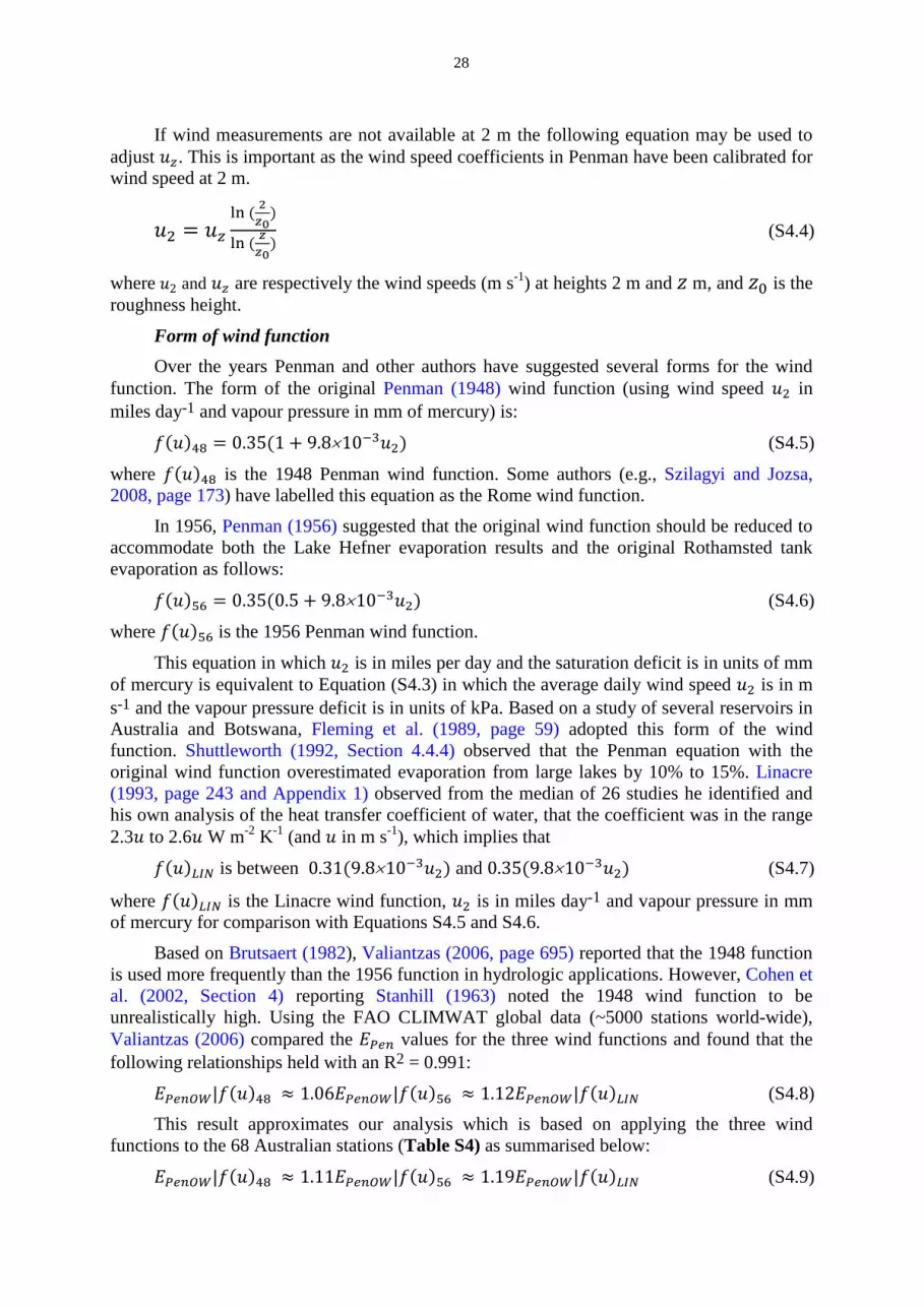
28

If wind measurements are not available at 2 m the following equation may be used to adjust 𝑢𝑧. This is important as the wind speed coefficients in Penman have been calibrated for wind speed at 2 m.

𝑢2 = 𝑢𝑧ln ( 2𝑧0

)

ln ( 𝑧𝑧0) (S4.4)

where 𝑢2 and 𝑢𝑧 are respectively the wind speeds (m s-1) at heights 2 m and 𝑧 m, and 𝑧0 is the roughness height.

Form of wind function Over the years Penman and other authors have suggested several forms for the wind

function. The form of the original Penman (1948) wind function (using wind speed 𝑢2 in miles day-1 and vapour pressure in mm of mercury) is:

𝑓(𝑢)48 = 0.35(1 + 9.8×10−3𝑢2) (S4.5)

where 𝑓(𝑢)48 is the 1948 Penman wind function. Some authors (e.g., Szilagyi and Jozsa, 2008, page 173) have labelled this equation as the Rome wind function.

In 1956, Penman (1956) suggested that the original wind function should be reduced to accommodate both the Lake Hefner evaporation results and the original Rothamsted tank evaporation as follows:

𝑓(𝑢)56 = 0.35(0.5 + 9.8×10−3𝑢2) (S4.6)

where 𝑓(𝑢)56 is the 1956 Penman wind function.

This equation in which 𝑢2 is in miles per day and the saturation deficit is in units of mm of mercury is equivalent to Equation (S4.3) in which the average daily wind speed 𝑢2 is in m s-1 and the vapour pressure deficit is in units of kPa. Based on a study of several reservoirs in Australia and Botswana, Fleming et al. (1989, page 59) adopted this form of the wind function. Shuttleworth (1992, Section 4.4.4) observed that the Penman equation with the original wind function overestimated evaporation from large lakes by 10% to 15%. Linacre (1993, page 243 and Appendix 1) observed from the median of 26 studies he identified and his own analysis of the heat transfer coefficient of water, that the coefficient was in the range 2.3𝑢 to 2.6𝑢 W m-2 K-1 (and 𝑢 in m s-1), which implies that

𝑓(𝑢)𝐿𝐼𝑁 is between 0.31(9.8×10−3𝑢2) and 0.35(9.8×10−3𝑢2) (S4.7)

where 𝑓(𝑢)𝐿𝐼𝑁 is the Linacre wind function, 𝑢2 is in miles day-1 and vapour pressure in mm of mercury for comparison with Equations S4.5 and S4.6.

Based on Brutsaert (1982), Valiantzas (2006, page 695) reported that the 1948 function is used more frequently than the 1956 function in hydrologic applications. However, Cohen et al. (2002, Section 4) reporting Stanhill (1963) noted the 1948 wind function to be unrealistically high. Using the FAO CLIMWAT global data (~5000 stations world-wide), Valiantzas (2006) compared the 𝐸𝑃𝑒𝑛 values for the three wind functions and found that the following relationships held with an R2 = 0.991:

𝐸𝑃𝑒𝑛𝑂𝑊|𝑓(𝑢)48 ≈ 1.06𝐸𝑃𝑒𝑛𝑂𝑊|𝑓(𝑢)56 ≈ 1.12𝐸𝑃𝑒𝑛𝑂𝑊|𝑓(𝑢)𝐿𝐼𝑁 (S4.8) This result approximates our analysis which is based on applying the three wind

functions to the 68 Australian stations (Table S4) as summarised below:

𝐸𝑃𝑒𝑛𝑂𝑊|𝑓(𝑢)48 ≈ 1.11𝐸𝑃𝑒𝑛𝑂𝑊|𝑓(𝑢)56 ≈ 1.19𝐸𝑃𝑒𝑛𝑂𝑊|𝑓(𝑢)𝐿𝐼𝑁 (S4.9)

29

Table S4 also shows a comparison with FAO-56 Reference Crop evapotranspiration and Priestley-Taylor evaporation as well as 10th and 90th percentile values.

Valiantzas (2006, page 696) suggested the 1948 wind function be adopted as standard in the Penman equation, however, noting the comments above by Shuttleworth (1992, Section 4.4.4), Linacre (1993) and Cohen et al (2002), we have adopted the Penman (1956) form of the wind function in this paper. In terms of the units used (vapour pressure in kPa, and mean daily wind speed in m s-1), the Penman 1956 wind function is:

𝑓(𝑢) = 1.313 + 1.381𝑢2 (S4.10)

For comparison, Penman’s 1948 wind function in the same units as Equation (S4.10) (vapour pressure in kPa, and wind speed in m s-1) is:

𝑓(𝑢) = 2.626 + 1.381𝑢2 (S4.11)

Penman equation without wind data Valiantzas (2006, Equation 33) proposed the following equation for situations where no

wind data are available:

𝐸𝑃𝑒𝑛𝑂𝑊 ≈ 0.047𝑅𝑆(𝑇𝑎 + 9.5)0.5 − 2.4 �𝑅𝑠𝑅𝑎�2

+ 0.09(𝑇𝑎 + 20) �1 − 𝑅𝐻𝑚𝑒𝑎𝑛100

� (S4.12)

where 𝐸𝑃𝑒𝑛𝑂𝑊 is Penman’s open-water evaporation (mm day-1), 𝑅𝑠 is the measured or estimated incoming solar radiation (MJ m-2 day-1), 𝑇𝑎 is the mean daily temperature (°C), 𝑅𝑎 is the extraterrestrial solar radiation (MJ m-2 day-1) and 𝑅𝐻𝑚𝑒𝑎𝑛 is the mean daily relative humidity (%). This assumes the albedo for water is 0.08 and the “0.09” in Equation (S4.12) applies to the Penman (1948) wind function. If one uses the Penman (1956) wind function, “0.09” should be replaced by “0.06”. Based on six years of daily data from California, Valiantzas (2006) compared Equation (S4.12) with Equation (S4.1) using monthly data and found the modified equation performed satisfactorily (R2 = 0.983, the long term ratio of “approximate” to “reference” evaporation was 0.995, and SEE = 0.25 mm day-1) compared with the standard Penman equation.

Modifying Penman equation by including aerodynamic turbulence According to Fennessey (2000), van Bavel (1966) modified the original Penman 1948

equation to take into account boundary layer resistance as follows:

𝐸𝑃𝑜𝑡𝑂𝑊′ = ∆∆+𝛾

𝑅𝑛−𝐺𝜆

+ 𝛾∆+𝛾

ρ𝑎𝑐𝑎(𝑣𝑎∗−𝑣𝑎)

𝜆𝑟𝑎 (S4.13)

where 𝐸𝑃𝑜𝑡𝑂𝑊′ is the modified Penman open water evaporation (mm day-1) incorporating aerodynamic resistance, 𝜌𝑎 is the mean air density at constant pressure (kg m-3), 𝑐𝑎 is the specific heat of the air (MJ kg-1 °C-1), and 𝑟𝑎 is an “aerodynamic or atmospheric resistance” to water vapour transport (s m-1). Equation (S4.13) for open water is equivalent to the Penman-Monteith Equation (S5.1) with the surface resistance 𝑟𝑠 set to zero.

To estimate aerodynamic resistance, McJannet et al. (2008a) introduced a specific wind function incorporating lake area into the Calder and Neal (1984) aerodynamic resistance equation as follows:

𝑟𝑎 = 86400 𝜌𝑎𝑐𝑎

𝛾�5𝐴�0.05

(3.80+1.57𝑢10) (S4.14)

30

where 𝑟𝑎 is the aerodynamic resistance over a lake (s m-1), 𝐴 is the lake area (km2) 𝜌𝑎 is the mean air density at constant pressure (1.2 kg m-3), 𝑐𝑎 is the specific heat of the air (0.001013MJ kg-1 °C-1), 𝛾 is the psychrometric constant (0.0668 kPa °C-1 at mean sea-level pressure 101.3 kPa), 𝑢10 is the wind speed (m s-1) at 10 m height, yielding 𝑟𝑎 for a lake at sea-level as:

𝑟𝑎 = 410

�5𝐴�0.05

(1+0.413𝑢10) (S4.15)

It is noted here that 𝑟𝑎 is a function of wind speed as well as lake area.

Chin (2011, Equation 12) offered an alternative equation to estimate 𝑟𝑎 for wind speeds (𝑢2) (m s-1) measured at 2 m height and for no adjustment for lake area as follows:

𝑟𝑎 = 400(1+0.536𝑢2) (S4.16)

Price (1994) estimated 𝑟𝑎 for Lake Ontario, Canada during a six-week summer period in 1991. Based on 2015 samples he determined a mean value of 𝑟𝑎 = 201 ± 122 s m-1. The wide range of observed values is a function of wind-speed.

Estimating ∆ under extreme conditions McArthur (1992, page 306) explains the assumptions behind ∆ in the Penman equation

(Equation (S4.1)). Equation (S4.17) provides the physically correct estimate of ∆, which requires knowledge of the evaporating surface temperature (𝑇𝑠).

∆=�𝑣𝑇𝑠∗ −𝑣𝑇𝑎

∗ �(𝑇𝑠−𝑇𝑎) (S4.17)

However, because 𝑇𝑠 is generally unknown, ∆ is approximated as the slope of the saturated vapour pressure curve at air temperature as follows:

∆′= 𝑑𝑣𝑇∗

𝑑𝑇 evaluated at air temperature (𝑇𝑎) (S4.18)

In most practical situations ∆′ is an acceptable approximation to ∆ when the surface and air temperatures are close (McArthur (1992, page 306)). Under extreme conditions, high aerodynamic resistance, high humidity and low temperature, the surface and air temperatures diverge and this approximation breaks down (Paw U (1992, page 299)) and can lead to under-estimating evaporation by about 10% (Slatyer and McIlroy, 1961; Paw U and Gao, 1988). Milly (1991), McArthur (1992) and Paw U (1992) provide a discussion of alternate procedures to estimate evaporation under such conditions.

31

Supplementary Material Section S5 Penman-Monteith and FAO-56 Reference Crop models

The Penman-Monteith model defined below is usually adopted to estimate potential evapotranspiration, 𝐸𝑃𝑀 (mm day-1). The equation is based on Allen et al. (1998, Equation 3):

𝐸𝑇𝑃𝑀 = 1𝜆

Δ(𝑅𝑛−𝐺)+𝜌𝑎𝑐𝑎�𝑣𝑎∗ −𝑣𝑎�𝑟𝑎

Δ+𝛾�1+𝑟𝑠𝑟𝑎�

(S5.1)

where 𝐸𝑇𝑃𝑀 is the Penman-Monteith potential evapotranspiration (mm day-1), 𝑅𝑛 is the net radiation at the vegetated surface (MJ m-2 day-1) incorporating an albedo value appropriate for the evaporating surface (Table S3), 𝐺 is the soil heat flux (MJ m-2 day-1), 𝜌𝑎 is the mean air density at constant pressure (kg m-3), 𝑐𝑎 is the specific heat of the air (MJ kg-1 °C-1), 𝑟𝑎 is an “aerodynamic or atmospheric resistance” to water vapour transport, i.e., from the leaf surface to the atmosphere (s m-1) (Dunin and Greenwood, 1986, page 48), 𝑟𝑠 is a “surface resistance” term, that is the resistances from within the plant to the bulk leaf surfaces (s m-1) (Dunin and Greenwood, 1986, page 48), (𝑣𝑎∗ − 𝑣𝑎) is the vapour pressure deficit (kPa), 𝜆 is the latent heat of vaporization (MJ kg-1), ∆ is the slope of the vapour pressure curve (kPa °C-1) at air temperature, and 𝛾 is the psychrometric constant ( kPa °C-1). 𝐺 is defined as (Allen et al., 1998, Equation 41):

𝐺 = 𝑐𝑠𝑑𝑠 �𝑇𝑖−𝑇𝑖−1

∆𝑡� (S5.2)

where 𝑐𝑠 is the volumetric heat capacity of soil (MJ m-3 °C-1) (for an average soil moisture 𝑐𝑠 ≅ 2.1, Grayson et al., 1996, page 33), 𝑑𝑠 is the effective soil depth (m), 𝑇𝑖 and 𝑇𝑖−1 are the average air temperatures (°C) on day 𝑖 and i-1 respectively, and ∆𝑡 is time-step (day).

It is noted in Section 2.1.2 that Equation (S5.1) is based on simplifying assumptions to account for the fact that the temperature of the evaporating surface is unknown. References for readers wishing to follow up on this topic include Monteith (1965), Monteith (1981) and Raupach (2001). An aspect of this issue is discussed in the previous section dealing with Equation (S4.14).

Generally, for daily time-steps 𝐺 can be assumed to be negligible (Allen et al., 1998, page 68).

Values of aerodynamic resistance and surface (or canopy) resistance

𝑟𝑎, the aerodynamic resistance, controls the removal of water vapour from the plant surface under neutral stability conditions and is defined for an evaporating surface by Allen et al. (1998, Equation 4) as follows:

𝑟𝑎 =𝑙𝑛�𝑧𝑚−𝑑

𝑧𝑜𝑚�𝑙𝑛�

𝑧ℎ−𝑑𝑧𝑜ℎ

�

𝑘2𝑢𝑧 (S5.3)

where 𝑧𝑚 is the height of the wind instrument (m), 𝑧ℎ is the height of the humidity measurements (m), 𝑑 is the zero plane displacement height (m), 𝑧𝑜𝑚 is the roughness length governing momentum transfer (m), 𝑧𝑜ℎ is the roughness length governing transfer of heat and vapour (m), 𝑘 is von Kármán’s constant (0.41), and 𝑢𝑧 is the wind speed at height 𝑧𝑚 (m s-1).

According to Allen et al. (1998, page 21), for a wide range of crops, 𝑑 and 𝑧𝑜𝑚 can be estimated from the crop height (h) as:

32

𝑑 = 0.67ℎ, and (S5.4)

𝑧𝑜𝑚 = 0.123ℎ (S5.5)

and 𝑧𝑜ℎ can be approximated from:

𝑧𝑜ℎ = 0.1𝑧𝑜𝑚 (S5.6)

Some typical values of 𝑟𝑎 are listed in Table S2. According to Chin (2011, Equation 12), Equation (S5.3) and the following Equation

(S5.7), which is for water, are conventional practice for the PM equation.

𝑟𝑎 =4.72�𝑙𝑛�𝑧𝑚𝑧𝑜

�2�2

1+0.54𝑢𝑧 (S5.7)

where 𝑧𝑚 is the height of wind measurements and 𝑧𝑜 (roughness length) is:

𝑧𝑜 = (𝑣𝑒𝑔𝑒𝑡𝑎𝑡𝑖𝑜𝑛 ℎ𝑒𝑖𝑔ℎ𝑡)10

(S5.8)

For water 𝑧𝑜 = 0.001 m (Table S2).

𝑟𝑠, the surface resistance term, in vegetation represents bulk stomatal resistance or canopy resistance, which is a property of the plant type and its water stress level. This term controls the release of water to the plant or soil surface; some typical values of 𝑟𝑠 are listed in Table S2. For water, 𝑟𝑠 = 0.

According to Allen et al. (1998) 𝑟𝑠 is a combination of several resistances in series including soil, total leaf area (canopy) and stomatal resistances. This is a complex subject and well beyond the scope of this paper. Readers are referred to Monteith (1965) and Shuttleworth and Gurney (1990).

Again following Allen et al. (1998, Equation 5), an alternative definition of 𝑟𝑠 after Szeicz et al. (1969, Equation 9) is:

𝑟𝑠 = 𝑟𝑙𝐿𝐴𝐼𝑎𝑐𝑡𝑖𝑣𝑒

(S5.9)

where 𝑟𝑙 is the bulk stomatal resistance of a well-illuminated leaf (s m-1), and 𝐿𝐴𝐼𝑎𝑐𝑡𝑖𝑣𝑒 is the active (sunlit) leaf area index (m2 (of leaf area) m-2 (of soil surface)). It is further noted by Allen et al. (1998) that 𝑟𝑙 is influenced by climate, water availability and vegetation type. They provide a simple example for a grass reference crop as follows:

𝐿𝐴𝐼𝑎𝑐𝑡𝑖𝑣𝑒 = 0.5𝐿𝐴𝐼, and (S5.10) and a general equation for LAI of grass is:

𝐿𝐴𝐼 = 24ℎ (S5.11)

where ℎ is the crop height (m).

Given the stomatal resistance of a single leaf of grass is ~100 s m-1 and the crop height is 0.12 m (Allen et al., 1998, page 22), then 𝑟𝑠 for a grass reference surface is:

𝑟𝑠 = 1000.5×24×0.12

= 70 s m-1 (S5.12)

Dingman (1992, page 296, footnote 9) notes that atmospheric conductance, 𝐶𝑎𝑡𝑚, is the inverse of aerodynamic resistance:

𝐶𝑎𝑡𝑚 = 1𝑟𝑎

(S5.13)

33

Also, it is implied from Dingman (1992, page 299) that canopy conductance, 𝐶𝑐𝑎𝑛, is the inverse of surface resistance:

𝐶𝑐𝑎𝑛 = 1𝑟𝑠

(S5.14)

Based on data collected in the Amazonian forest, Shuttleworth (1988) proposed that for a dry canopy the surface resistance can be described by the following quadratic function of time of day, with 𝑟𝑠 falling to a minimum late morning and rising to a very large value at dusk as follows:

𝑟𝑠 = 1000

12.17−0.531�𝑡𝑑𝑎𝑦−12�−0.223�𝑡𝑑𝑎𝑦−12�2 (S5.15)

where 𝑟𝑠 is surface or canopy resistance (s m-1) and 𝑡𝑑𝑎𝑦 is local time of day in hours.

Readers interested in this topic are referred to Sharma (1984), Kelliher et al (1995), Magnani et al. (1998), Silberstein et al. (2003) and Amer and Hatfield (2004).

To understand the relative importance of radiation and atmospheric demand (through the vapour pressure deficit) in the transpiration process, Jarvis and McNaughton (1986, A16) introduced a decoupling coefficient, Ω, (Equation S5.16) which ranges between 0 and 1 and is a measure of the decoupling between the conditions at the surface of a leaf and in the surrounding air:

Ω =Δ𝛾+1

Δ𝛾+1+

𝑟𝑠𝑟𝑎

(S5.16)

Wallace and McJannet (2010, page 109) explain the significance of Ω as follows. When Ω is small there is a strong coupling between the canopy and the atmosphere and, consequently, canopy conductance, the vapour pressure deficit and wind speed strongly influence transpiration, whereas as Ω approached 1 (complete decoupling) radiation is the dominant factor affecting transpiration. This relationship is explained mathematically by Kumagai et al (2004, Equation 3) as follows:

𝐸𝑇𝑃𝑀 = Ω𝐸1𝑠𝑡 + (1 − Ω)𝐸2𝑛𝑑 (S5.17)

where 𝐸1𝑠𝑡 is the radiation (first) term in the PM model (Equation S5.1) and 𝐸2𝑛𝑑 is aerodynamic (second) term.

FAO-56 Reference Crop Evapotranspiration

If we substitute for 𝑟𝑎 and 𝑟𝑠 in Equation (S5.1) using the relevant equations in Allen et al. (1998, Equations (3) and (4)) and adopting the properties of the FAO-56 hypothetical crop of assumed height of 0.12 m, a surface resistance of 70 s m-1 and an albedo of 0.23, the substitutions yield the familiar FAO-56 Reference Crop evapotranspiration, 𝐸𝑇𝑅𝐶, equation (Allen et al., 1998, Equation 6):

𝐸𝑇𝑅𝐶 =0.408Δ(Rn−G)+γ 900

Ta+273u2(𝑣𝑎∗−𝑣𝑎)

Δ+γ(1+0.34u2) = 𝐸𝑇𝑅𝐶𝑠ℎ (S5.18)

where 𝐸𝑇𝑅𝐶𝑠ℎ is the Reference Crop evapotranspiration for short grass (mm day-1), u2 is the average daily wind speed (m s-1) at 2 m, and Ta is the mean daily air temperature (°C). Meyer (1999) discusses the application of the Penman-Monteith equation to inland south-eastern Australia.

ASCE-EWRI Standardized Penman-Monteith Equation

34

The ASCE-EWRI Standardized Penman-Monteith Equation (S5.19) (ASCE, 2005, Equation 1, Table 1) was developed to estimate potential evapotranspiration from a tall crop with the following characteristics: vegetation height 0.50 m, surface resistance 45 s m-1 and albedo of 0.23. The equivalent equation to Equation (S5.18) for tall grass is:

𝐸𝑇𝑅𝐶𝑡𝑎 =0.408Δ(Rn−G)+γ 1600

Ta+273u2(𝑣𝑎∗−𝑣𝑎)

Δ+γ(1+0.38u2) (S5.19)

where 𝐸𝑇𝑅𝐶𝑡𝑎 is the Reference Crop evapotranspiration for tall grass (mm day-1).

Adjustment for height of wind speed measurement in Penman-Monteith and FAO-56 Reference Crop equations

The following equation is to adjust wind speed for instrument height associated with short grassed surfaces (Allen et al., 1998, Equation (47)):

𝑢2 = 𝑢𝑧4.87

𝑙𝑛(67.8𝑧−5.42) (S5.20)

where 𝑢2 and 𝑢𝑧 are respectively the wind speeds at heights 2 m and z m.

Reference Crop equation without wind data Valiantzas (2006, Equation 39) proposed the following equation (which is similar to the

simplified Penman equation, see Equation (S4.12)), to estimate monthly Reference Crop evapotranspiration for situations where no wind data are available:

𝐸𝑇𝑅𝐶 ≈ 0.038𝑅𝑆(𝑇� + 9.5)0.5 − 2.4 �𝑅𝑆𝑅𝐴�2

+ 0.075(𝑇� + 20) �1 − 𝑅𝐻100� (S5.21)

where 𝐸𝑇𝑅𝐶 is the Reference Crop estimate of evapotranspiration for short grass (mm day-1), 𝑅𝑆 is the measured or estimated average monthly incoming solar radiation (MJ m-2 day-1), 𝑇� is the mean monthly air temperature (°C), 𝑅𝐴 is the average monthly extraterrestrial solar radiation (MJ m-2 day-1) and 𝑅𝐻 is the mean monthly relative humidity (%). This procedure assumes the albedo = 0.25 (rather than the standard 0.23) for a crop. For 535 northern hemisphere climate stations, monthly estimates of 𝐸𝑅𝐶 based on Equation (S5.21) were compared with the standard reference crop Equation (S5.18). The approximate model performed very well on a sub-set of 4461 monthly estimates (R2 = 0.951), the long term ratio of “approximate” to “reference” was 1.03, and SEE = 0.34 mm day-1.

Application of Penman-Monteith to water bodies based on equilibrium temperature An interesting application of the Penman-Monteith equation (Equation (S5.1) to a range

of water bodies (irrigation channels, ponds, lakes, reservoirs streams and floodplains) was carried out by McJannet et al. (2008b) who set 𝑟𝑠 = 0 for water bodies (Table S2). The approach is outlined in Section S11.

Shuttleworth-Wallace To deal with sparse vegetation Shuttleworth and Wallace (1985, Equations 11 to 18)

modified the PM model to separate evapotranspiration into soil evaporation and transpiration. Wessel and Rouse (1994) further modified the Shuttleworth-Wallace (SW) model to accommodate evaporation from water surfaces but recommended that this component be not included in the SW approach. The Shuttleworth and Wallace (1985) equations are:

𝐸𝑆𝑊 = 1𝜆

(𝐶𝑐𝑎𝑃𝑀𝑐𝑎 + 𝐶𝑠𝑢𝑃𝑀𝑠𝑢) (S5.22)

35

𝑃𝑀𝑐𝑎 = 1𝜆

∆𝐴𝑒+�𝜌𝑐𝑎�𝑣𝑎

∗ −𝑣𝑎�−∆𝑟𝑎𝑐𝐴𝑠𝑠�

𝑟𝑎𝑎+𝑟𝑎

𝑐

∆+𝛾�1+ 𝑟𝑠𝑐


𝑐 � (S5.23)

𝑃𝑀𝑠𝑢 = 1𝜆

∆𝐴𝑒+�𝜌𝑐𝑎�𝑣𝑎

∗ −𝑣𝑎�−∆𝑟𝑎𝑠 (𝐴𝑒−𝐴𝑠𝑠)�


𝑠

∆+𝛾�1+ 𝑟𝑠𝑠


𝑠 � (S5.24)

𝐶𝑐𝑎 = 1�1+ 𝜂𝑐𝜂𝑎

𝜂𝑠(𝜂𝑐+𝜂𝑎)� (S5.25)

𝐶𝑠𝑢 = 1�1+ 𝜂𝑠𝜂𝑎

𝜂𝑐(𝜂𝑠+𝜂𝑎)� (S5.26)

𝜂𝑎 = (∆ + 𝛾)𝑟𝑎𝑎 (S5.27)

𝜂𝑠 = (∆ + 𝛾)𝑟𝑎𝑠 + 𝛾𝑟𝑠𝑠 (S5.28)

𝜂𝑐 = (∆ + 𝛾)𝑟𝑎𝑐 + 𝛾𝑟𝑠𝑐 (S5.29)

where 𝐸𝑆𝑊 is the Shuttleworth-Wallace combined evaporation (mm day-1) from the vegetation and the soil, 𝑃𝑀𝑐𝑎 and 𝑃𝑀𝑠𝑢 are respectively the evaporation (mm day-1) from a closed canopy and from bare substrate, 𝐴𝑒 is the available energy (MJ m-2 day-1) defined as the above-canopy fluxes of sensible heat and latent heat, and 𝐴𝑠𝑠 is the energy (MJ m-2 day-1) available at the substrate, 𝜆 is the latent heat of vaporization (MJ kg-1), ∆ is the slope of the vapour pressure curve (kPa °C-1), 𝛾 is the psychrometric constant (kPa °C-1), 𝑐𝑎 is the specific heat of the air (MJ kg-1 °C-1) at air temperature, (𝑣𝑎∗ − 𝑣𝑎) is the vapour pressure deficit (kPa), 𝑟𝑎𝑎 is the aerodynamic resistance between the canopy source height and the reference level (s m-1), 𝑟𝑎𝑐 is the bulk boundary layer resistance of the vegetative elements in the canopy level (s m-1), 𝑟𝑎𝑠 is the aerodynamic resistance between the substrate and canopy source height level (s m-1), 𝑟𝑠𝑐 is the bulk stomatal resistance of the canopy level (s m-1), and 𝑟𝑠𝑠 is the surface resistance of the substrate level (s m-1). Wessel and Rouse (1994, Section 4.1) were unable to determine the soil surface resistance, 𝑟𝑠, and adopted a value of 500 s m-1 for their hourly analysis.

It appears that Shuttleworth and Wallace (1985) did not prescribe the appropriate time-step that should be used in their model but Wessel and Rouse (1994) adopted both an hourly and daily time-step in their simulations. Readers interested in applying the SW model should refer to Stannard (1993) and Federer et al. (1996).

Weighted Penman-Monteith In order to estimate the evaporation from a wetland, Wessel and Rouse (1994, Equation

14) proposed the following weighted Penman-Monteith approach:

𝐸𝑤𝑒𝑡𝑙𝑎𝑛𝑑 = 𝐿𝐴𝐼 𝐸𝑐𝑎𝑛 + 𝑆 𝐸𝑠𝑜𝑖𝑙 + 𝑊 𝐸𝑤𝑎𝑡𝑒𝑟 (S5.30)

where 𝐸𝑤𝑒𝑡𝑙𝑎𝑛𝑑 is the evapotranspiration (mm day-1) from the wetland, 𝐸𝑐𝑎𝑛 is the transpiration (mm day-1) from the canopy, 𝐸𝑠𝑜𝑖𝑙 is the soil evaporation (mm day-1), 𝐸𝑤𝑎𝑡𝑒𝑟 is the evaporation (mm day-1) from the standing water, 𝐿𝐴𝐼 is the leaf area index, and S and W are respectively the proportion of total area of bare soil and open water. 𝐸𝑐𝑎𝑛, 𝐸𝑠𝑜𝑖𝑙 and 𝐸𝑤𝑎𝑡𝑒𝑟 are the Penman-Monteith estimates of ET for the canopy, soil and water as specified by Drexler et al. (2004, Equations 17 to 19):

36

𝐸𝑐𝑎𝑛 = 1𝜆

∆(𝑅𝑛𝑐𝑎𝑛−𝐺)+𝜌𝑐𝑎�𝑣𝑎∗ −𝑣𝑎� 𝑟𝑎

Δ+𝛾�1+𝑟𝑐𝑟𝑎�

(S5.31)

𝐸𝑠𝑜𝑖𝑙 = 1𝜆

∆�𝑅𝑛𝑠𝑜𝑖𝑙−𝐺�+𝜌𝑐𝑎�𝑣𝑎

∗ −𝑣𝑎� 𝑟𝑎

Δ+𝛾�1+𝑟𝑠𝑠

𝑟𝑎�

(S5.32)

𝐸𝑤𝑎𝑡𝑒𝑟 = 1𝜆

∆�𝑅𝑛𝑤𝑎𝑡𝑒𝑟−𝐺�+𝜌𝑐𝑎�𝑣𝑎

∗ −𝑣𝑎� 𝑟𝑎

Δ+𝛾 (S5.33)

where 𝐸𝑐𝑎𝑛, 𝐸𝑠𝑜𝑖𝑙, and 𝐸𝑤𝑎𝑡𝑒𝑟 are respectively the evaporation (mm day-1) from the canopy, soils and water, 𝑅𝑛𝑐𝑎𝑛, 𝑅𝑛𝑠𝑜𝑖𝑙, and 𝑅𝑛𝑤𝑎𝑡𝑒𝑟 are respectively the net solar radiation (MJ m-2 day-1) to the canopy, soil and water, 𝐺 is the heat flux transfer (MJ m-2 day-1) to and from the soil and water, and other variables are defined above.

Matt-Shuttleworth Shuttleworth and Wallace (2009, page 1904) recommend that the FAO-56 Reference

Crop method (Allen et al., 1998) should not be applied to irrigation areas like those in Australia that are semi-arid and windy. They recommend that the Matt-Shuttleworth (M-S) model be adopted in place of the FAO-56 Reference Crop method. The M-S model consists of five steps (details are given in Shuttleworth and Wallace (2009, as Equations 5, 8, 9, and 10):

1. Select the surface resistance for the target crop (from Shuttleworth and Wallace (2009, Table 3). For example, for rye grass the surface resistance is 66 s m-1.

2. Calculate

𝑟𝑐𝑙𝑖𝑚 = 86400 𝜌𝑎𝑐𝑎(𝑉𝑃𝐷)∆𝑅𝑛

(S5.34)

where 𝑟𝑐𝑙𝑖𝑚 is termed the climatological resistance (s m-1), 𝜌𝑎 is the mean air density (kg m-3) at constant pressure, 𝑐𝑎 is the specific heat of the air (MJ kg-1 °C-1), (𝑉𝑃𝐷) is the vapour pressure deficit (kPa), ∆ is the slope of the vapour pressure curve (kPa °C-1) at air temperature, and 𝑅𝑛 is the net radiation (MJ m-2 day-1) at the vegetated surface. The 86,400 constant converts the radiation energy from MJ m-2 day-1 to MJ m-2 sec-1.

3. Calculate

𝑉𝑃𝐷50𝑉𝑃𝐷2

= �302(∆+𝛾)+70𝛾𝑢2208(∆+𝛾)+70𝛾𝑢2

� + 1𝑟𝑐𝑙𝑖𝑚

��302(∆+𝛾)+70𝛾𝑢2208(∆+𝛾)+70𝛾𝑢2

� �208𝑢2� − �302

𝑢2�� (S5.35)

where 𝑉𝑃𝐷50 and 𝑉𝑃𝐷2 are the vapour pressure deficits (kPa) at 50 m and 2 m height, and 𝑢2 is the mean daily wind speed (m s-1) at 2 m height.

4. Calculate

𝑟𝑐50 = 1(0.41)2 𝑙𝑛 �

(50−0.67ℎ)(0.123ℎ) � 𝑙𝑛 �

(50−0.67ℎ)(0.0123ℎ) �

𝑙𝑛�(2−0.08)0.0148 �

𝑙𝑛�(50−0.08)0.0148 �

(S5.36)

where 𝑟𝑐50 is the aerodynamic coefficient (s m-1) for crop height (ℎ)

5. Calculate

𝐸𝑇𝑐 = 1𝜆

∆𝑅𝑛+𝜌𝑎𝑐𝑎𝑢2(𝑉𝑃𝐷2)

𝑟𝑐50 � 𝑉𝑃𝐷50𝑉𝑃𝐷2

�

∆+𝛾�1+(𝑟𝑠)𝑐𝑢2𝑟𝑐50 �

(S5.37)

37

where 𝐸𝑇𝑐 is the well-watered crop evapotranspiration in a semi-arid and windy location, 𝜆 is the latent heat of vaporization (MJ kg-1), (𝑟𝑠)𝑐 is the surface resistance (s m-1) of a well-watered crop equivalent to the FAO crop coefficient (Shuttleworth and Wallace, 2009, Table 3), and other variables are defined previously.

At five locations in Australia, Shuttleworth and Wallace (2009) compared water requirements estimated by the Matt-Shuttleworth method with the requirements estimated by FAO-56 Reference Crop method (Allen et al., 1998, Chapter 4) for irrigated sugar cane, cotton and short pasture. The analysis showed that within a growing season the differences between the two procedures varied considerably. However, over an entire season the M-S evapotranspiration estimate was 3% to 15% higher for sugar cane, 6% higher for cotton and between 0.5% and 2.5% for pasture compared to the FAO-56 method (Shuttleworth and Wallace, 2009, Table 4 and page 1905).

38

Supplementary Material Section S6 PenPan model

There have been several variations of the Penman equation to model the evaporation from a Class-A evaporation pan. Linacre (1994) developed a physical model which he called the Penpan formula or equation. Rotstayn et al. (2006) coupled the radiative component of Linacre (1994) and the aerodynamic component of Thom et al. (1981) to develop the PenPan model which is defined, using the symbols of Johnson and Sharma (2010), as follows:

𝐸𝑃𝑒𝑛𝑃𝑎𝑛 = ∆∆+𝑎𝑝𝛾

𝑅𝑁𝑃𝑎𝑛𝜆

+ 𝑎𝑝𝛾∆+𝑎𝑝𝛾

𝑓𝑃𝑎𝑛(𝑢)(𝑣𝑎∗ − 𝑣𝑎) (S6.1)

where 𝐸𝑃𝑒𝑛𝑃𝑎𝑛 is the modelled Class-A (unscreened) pan evaporation (mm day-1), 𝑅𝑁𝑃𝑎𝑛 is the net radiation (MJ m-2 day-1) at the pan, ∆ is the slope of the vapour pressure curve (kPa °C-1) at air temperature, 𝛾 is the psychrometric constant (kPa °C-1), and 𝜆 is the latent heat of vaporization (MJ kg-1), 𝑎𝑝 is a constant adopted as 2.4, 𝑣𝑎∗ − 𝑣𝑎 is the vapour pressure deficit (kPa), and 𝑓𝑃𝑎𝑛(𝑢) is defined as (Thom et al., 1981, Equation 34):

𝑓𝑃𝑎𝑛(𝑢) = 1.201 + 1.621 𝑢2 (S6.2)

where 𝑢2 is the average daily wind speed at 2 m height (m s-1).

To estimate 𝑅𝑁𝑃𝑎𝑛, we refer to Rotstayn et al. (2006, Equations 4 and 5)):

𝑅𝑁𝑃𝑎𝑛 = (1 − 𝛼𝐴)𝑅𝑆𝑃𝑎𝑛 − 𝑅𝑛𝑙 (S6.3)

𝑅𝑆𝑃𝑎𝑛 = [𝑓𝑑𝑖𝑟𝑃𝑟𝑎𝑑 + 1.42(1 − 𝑓𝑑𝑖𝑟) + 0.42𝛼𝑠𝑠]𝑅𝑆 (S6.4)

where 𝑅𝑆𝑃𝑎𝑛 is the total shortwave radiation (MJ m-2 day-1) received by the pan, 𝑅𝑛𝑙 is the net outgoing longwave radiation (MJ m-2 day-1) from the pan, 𝑅𝑆 is the incoming solar radiation (shortwave) (MJ m-2 day-1) at the surface, 𝑓𝑑𝑖𝑟 is the fraction of 𝑅𝑆 that is direct, 𝑃𝑟𝑎𝑑 is a pan radiation factor, 𝛼𝐴 is the albedo for a Class-A pan given as 0.14 (Linacre, 1992) as reported by Rotstayn et al. (2006, page 2), and 𝛼𝑠𝑠 is the albedo of the ground surface surrounding the evaporation pan (Table S3). To be consistent with Equation (S3.1) we have assumed the net outgoing longwave radiation 𝑅𝑛𝑙 as positive. As noted by Roderick et al. (2007, page 1), 𝑅𝑆𝑃𝑎𝑛 > 𝑅𝑆 because of the interception of energy by the pan walls.

𝑓𝑑𝑖𝑟 and 𝑃𝑟𝑎𝑑 are defined as:

𝑓𝑑𝑖𝑟 = −0.11 + 1.31 𝑅𝑆𝑅𝑎

(S6.5)

𝑃𝑟𝑎𝑑 = 1.32 + 4 × 10−4𝑙𝑎𝑡 + 8 × 10−5𝑙𝑎𝑡2 (S6.6)

where 𝑅𝑎 is the extraterrestrial radiation (MJ m-2 day-1), and 𝑙𝑎𝑡 is the absolute value of latitude in degrees.

The equations to estimate 𝑅𝑛𝑙 are set out in Section S3. The above analysis is carried out on a monthly time-step.

Application to Australian data

Using the PenPan model (with 𝑎𝑠 = 0.23 and 𝑏𝑠 = 0.50 as noted in Section S3), the mean monthly ratio of the PenPan evaporation, adjusted for the bird-screen, to the Class-A pan evaporation over the 68 stations (consisting of approximately 11840 ratios over all months) is 1.078. The monthly evaporation estimates are plotted in Figure S3. The performance of the PenPan model in estimating Class-A pan evaporation is satisfactory

39

although the PenPan values are biased towards slightly higher values at lower evaporations. These results compare favourably with PenPan versus Class-A pan evaporation results of Rotstayn et al. (2006, Figure 4), Roderick et al. (2007, Figure 1) and Johnson and Sharma (2010, Figure 1) especially as we use the standard climate data available through the Bureau of Meteorology National Climate Centre and sunshine hours as the basis of estimating solar radiation.

An objective of this supplementary material was to develop for Australia mean monthly evaporation pan coefficients (relating open surface-water based on Penman to Class-A pan evaporation). Confidence in the monthly Penman estimates is based on the fact that the PenPan estimates, which utilise the same climatic data and a similar model structure as for the Penman model, were found to estimate the monthly pan evaporation very satisfactorily. In order to estimate Penman evaporation suitable for computing pan coefficients, we varied 𝑎𝑠 and 𝑏𝑠 values so that the overall monthly PenPan/Class-A pan ratio for the 68 stations was unity. We argue that the optimised values of 𝑎𝑠 = 0.05 and 𝑏𝑠 = 0.65 obtained in this way provided realistic monthly Penman values and, therefore, realistic pan coefficients. The mean monthly pan coefficients for the 68 Australian stations are listed in Table S6.

40

Supplementary Material

Section S7 Morton models In 1985, Morton et al. (1985) published the program WREVAP which sets out

operational aspects for computing estimates of areal evapotranspiration and lake evaporation. WREVAP contains three models CRAE (Complementary Relationship Areal Evapotranspiration) (Morton, 1983a), CRWE (Complementary Relationship Wet-Surface Evaporation) (Morton, 1983b) and CRLE (Complementary Relationship Lake Evaporation) (Morton, 1986). CRAE computes evapotranspiration for the land-based environment whereas CRWE deals with shallow lakes and CRLE considers deep lakes where water-borne heat input and energy storage are key issues. The three models are shown comparatively in Table 2 and are described in detail below.

In Morton’s procedure, measurements of solar radiation are not required but are estimated through sunshine duration. However, if solar radiation data are available they may be used. The climate variables necessary to compute Morton’s monthly evaporation are mean monthly maximum and minimum air temperature, dew point temperature (or monthly relative humidity), monthly sunshine duration and mean annual rainfall. For periods shorter than one month, Morton (1983a, page 28) imposed a limit on the shortest time-step for analysis and advocated a minimum of five days. However, for hydrological applications, Morton (1986, page 379) permits daily time-step analysis so long as the daily values are accumulated to a week or longer. But, it is important for lake analysis, described in CRLE below, that the time-step of analysis be one month (Morton (1986, page 379).

Morton (1986, page 378) notes that the CRLE model estimates are sensitive to radiation inputs (or sunshine hours) but insensitive to errors in air temperature and relative humidity inputs, whereas the CRAE model requires accurate air temperature and relative humidity from a representative location. For lakes, land-based meteorological data can be used (Morton, 1983b, page 82). Furthermore, Morton (1986, page 378) notes that data measured over water have only a “…relatively minor effect…” on the estimate of lake evaporation.

CRAE The CRAE model consists of three components: potential evapotranspiration, wet-

environment areal evapotranspiration and actual areal evapotranspiration. A discussion of each component follows.

Estimating potential evapotranspiration (𝐸𝑇𝑃𝑜𝑡 in Figure 1) Morton’s approach to estimating potential evapotranspiration for a catchment or a large

vegetated surface is to solve the energy-balance and the vapour transfer equations respectively for potential evapotranspiration and the equilibrium temperature:

𝐸𝑇𝑃𝑜𝑡𝑀𝑜 = 1𝜆�𝑅𝑛 − [𝛾𝑝𝑓𝑣 + 4𝜖𝑠𝜎(𝑇𝑒 + 273)3](𝑇𝑒 − 𝑇𝑎)� (S7.1)

𝐸𝑇𝑃𝑜𝑡𝑀𝑜 = 1𝜆�𝑓𝑣(𝑣𝑒∗ − 𝑣𝐷∗ )� (S7.2)

where 𝐸𝑇𝑃𝑜𝑡𝑀𝑜 is Morton’s estimate of point potential evapotranspiration (mm day-1), 𝑅𝑛 is the net radiation (W m-2) for soil-plant surfaces at air temperature, 𝛾 is the psychrometric constant (mbar °C-1), 𝑝 is the atmospheric pressure (mbar), 𝑓𝑣 is a vapour transfer coefficient (W m-2 mbar-1), 𝜖𝑠 is the surface emissivity, 𝜎 is the Stefan-Boltzmann constant (W m-2 K-4), 𝑇𝑒 and 𝑇𝑎 are the equilibrium and air temperatures (°C), 𝑣𝑒∗ is the saturation vapour pressure

41

(mbar) at 𝑇𝑒, 𝑣𝐷∗ is the saturation vapour pressure (mbar) at dew point temperature, and 𝜆 is the latent heat of vaporisation (W day kg-1). (Note, the units used in Morton’s procedures have been adopted here to ensure that the correct values of the empirical constants are included.)

𝑓𝑣 is given by:

𝑓𝑣 = �𝑝𝑠𝑝�0.5 𝑓𝑧

𝜉 (S7.3)

where 𝑝𝑠 and 𝑝 are the sea-level atmospheric pressure (mbar) and at-site atmospheric pressure (mbar) respectively, 𝑓𝑍 is a constant (W m-2 mbar-1), and 𝜉 is a dimensionless stability factor estimated from:

𝜉 = 1

0.28�1+𝑣𝐷∗

𝑣𝑎∗ �+

𝑅𝑛∆

�𝛾𝑝�𝑝𝑠𝑝 �0.5

𝑏0𝑓𝑧�𝑣𝑎∗ −𝑣𝐷

∗ ��

noting that 𝜉 ≥ 1 (S7.4)

where 𝑣𝐷∗ is the saturation vapour pressure (mbar) at dew point temperature, 𝑣𝑎∗ is the saturation vapour pressure (mbar) at air temperature, ∆ is the slope of the saturation vapour pressure curve (mbar °C-1) at air temperature, and 𝑏0 = 1.0 for the CRAE model (Table 2).

We note here that 𝑓𝑣 is independent of wind speed. Many procedures (Penman, FAO-56 Reference Crop, PenPan, Advection-Aridity) used for estimating evaporation require wind as an input variable. However, Morton (1983b, page 95) argued that using routinely observed wind speeds in estimating lake evaporation do not significantly reduce the error in evaporation estimates. Based on three arguments ((1) the vapour transfer coefficient increases with increases in both surface roughness and wind speed yet wind speed tends to be lower in rough areas than in smooth areas, (2) 𝑓𝑣 increases with atmospheric instability and is more pronounced at low wind speeds than at high wind speeds, and (3) errors in wind measurements), he assumed that the vapour transfer coefficient is independent of wind speed (Morton 1983a, page 25).

Morton (1983a, Section 5.1) sets out the following procedure to find 𝑇𝑒 by iteration, and then 𝐸𝑃𝑜𝑡𝑀𝑂 can be estimated from Equation (S7.1). Assume a trial value of 𝑇𝑒′, which yields Δe′ and 𝛿𝑇𝑒 = 𝑇𝑒 − 𝑇𝑒′, hence 𝛿𝑣𝑒 = Δe′ 𝛿𝑇𝑒 and 𝑣𝑒∗′ = 𝑣𝑒

∗ + 𝛿𝑣𝑒. Equating Equations (S7.1) and (S7.2) and substituting gives:

𝛿𝑇𝑒 =𝑅𝑛𝑓𝑣+𝑣𝑎∗−𝑣𝑒∗′+𝜆𝑒�𝑇−𝑇𝑒′�

�Δe′ +𝜆𝑒� (S7.5)

where 𝜆𝑒 = 𝛾𝑝 + 4𝜖𝜎(𝑇𝑒+273)3

𝑓𝑣 (S7.6)

and variables are defined previously. Initially, 𝑇𝑒′ is set equal to the air temperature and the iterative procedure continues until

𝛿𝑇𝑒 becomes <0.01°C. Further details of the procedure are not included here but a worked example is provided in Section S21.

Estimating wet-environment areal evapotranspiration (𝐸𝑇𝑊𝑒𝑡 in Figure 1) To estimate the wet-environment areal evapotranspiration, which is equivalent to the

conventional definition of potential evapotranspiration, Morton added an empirically derived advection constant (𝑏1) to the Priestley-Taylor equation (Equation (6) with G = 0) as follows:

42

𝐸𝑇𝑊𝑒𝑡 𝑀𝑜 = 1

𝜆�𝑏1 + 𝑏2

𝑅𝑛𝑒�1+𝛾𝑝Δe

�� (S7.7)

where 𝐸𝑇𝑊𝑒𝑡 𝑀𝑜 is the wet-environment areal evapotranspiration (mm day-1), 𝑅𝑛𝑒 is the net

radiation (W m-2) for the soil-plant surface at 𝑇𝑒 (°C), Δe is the slope of the saturation vapour pressure curve (mbar °C-1) at 𝑇𝑒 (°C), 𝑏1 and 𝑏2 are empirical coefficients, and the other variables are as defined previously. Values of 𝑏1 and 𝑏2, which were derived by Morton (1983a, page 25) for representative regions, are set out in Table 2. 𝑅𝑛𝑒 is estimated as follows (Morton, 1983a, Equation C37):

𝑅𝑛𝑒 = 𝐸𝑇𝑃𝑜𝑡𝑀𝑜 + 𝛾𝑝𝑓𝑣(𝑇𝑒 − 𝑇𝑎) (S7.8)

In their analysis of Australian data, Wang et al. (2001) adopted after calibration 𝑓𝑍 = 29.2 Wm-2 mbar-1 (Equation (S7.3)) and 𝑏1 and 𝑏2(Equation S7.7) equal to 13.4 Wm-2 and 1.13 Wm-2 instead of 28 Wm-2 mbar-1, 14 Wm-2, and 1.2 Wm-2 respectively (Table 2) to give an overall value of the Priestley-Taylor coefficient, 𝛼𝑃𝑇, equal to 1.26 rather than Morton’s 1.32 value. Chiew and Leahy (2003, Section 2.3) argue that the recalibrated values better represent Australian data. Our analysis for Australia stations (to be reported in later document) confirms that the Wang et al. (2001) calibrated parameters yield more realistic results than those of Morton.

Estimating actual areal evapotranspiration (𝐸𝑇𝐴𝑐𝑡 in Figure 1)

To estimate Morton’s actual areal evapotranspiration (𝐸𝑇𝐴𝑐𝑡𝑀𝑜) (mm day-1), one uses the results from Equations (S7.1) and (S7.7) in the Complementary Relationship as follows:

𝐸𝑇𝐴𝑐𝑡𝑀𝑜 = 2𝐸𝑇𝑊𝑒𝑡 𝑀𝑜 − 𝐸𝑇𝑃𝑜𝑡𝑀𝑜 (S7.9)

Morton (1983a, page 29) argues that as the models are completely calibrated they are accurate world-wide.

Limitations of CRAE model Morton (1983a, page 28) points out five limitations of the CRAE model:

1. The model requires accurate measurements of humidity data. 2. The model should not be used for intervals of three days or less, however, as Morton

(1983a) notes, so long as the accumulated values for a week or longer are accurate then a daily time-step is acceptable. (For lake evaporation, a monthly time-step should be used (Morton et al., 1985)).

3. The CRAE model should not be used near sharp discontinuities, e.g., near the edge of an oasis.

4. The climatological station should be representative of the area of interest. 5. Because the CRAE model does not use knowledge about the soil-vegetation system,

it should not be used to examine the impact of natural or man-made change in the system.

Documentation of CRAE model Documentation of the detailed steps to apply the CRAE model is given in Morton

(1983a), Appendix C, and will not be repeated here. Our Section S21 provides a worked example.

CRWE In CRWE, the only difference to CRAE is that the radiation absorption and the vapour

transfer characteristics reflect the water surface rather than a vegetated surface (Morton,

43

1983b) (Table 2). The CRWE model provides estimates of lake-size wet surface evaporation from routine climate data observed in the land environment. Furthermore, according to Morton (1986, page 371) monthly evaporation can be accumulated to provide reliable estimates of lake evaporation at the annual time-step for lakes up to approximately 30 m deep. To estimate the evaporation from a shallow lake, Equation (S7.7) is applied with coefficients 𝑏1 and 𝑏2 taking values given in Table 2.

CRLE In the CRLE model, the computational procedure to estimate lake evaporation is the

same as that used in CRWE except that the energy term is net energy available, which depends on solar and water inputs for the current and previous months. In estimating deep lake evaporation on a monthly time-step, where changes in sub-surface heat storage may be important, Morton (1986, page 376) adopts a classical lag and route procedure where the routing is a linear storage function. The 1986 method, which we adopt herein, is different to Morton’s (1983b, Section 3) method. In the 1983 method, storage routing is applied to estimates of the shallow lake evaporation, whereas in Morton’s (1986) procedure, the solar and water borne inputs are routed and then lake evaporation is estimated. Using Morton’s symbols we summarise the four-step procedure of Morton (1986) as follows. Firstly, estimates of the solar and water borne heat input are computed:

𝐺𝑊0 = (1 − 𝛼)𝑅𝑠 − 𝑅𝑛𝑙 + δℎ (S7.10)

where 𝐺𝑊0 is the solar and waterborne heat input (W m-2), 𝑅𝑠 is the incident global radiation (W m-2), 𝑅𝑛𝑙 is the net outgoing longwave radiation (W m-2), 𝛼 is albedo for water, (1 −𝛼𝑅𝑠 is the net incoming shortwave radiation (W m-2), and δℎ, which is usually small, is the difference between heat content of inflows and outflows from the lake (W m-2). However, δℎ may be important for small lakes that receive cooling water with elevated temperatures, e.g., from a thermal power station or for a small deep lake with seasonal heat input from a large river (Morton, 1986, page 376). Note that Equation (S7.10) is different to Morton (1986, Equation 2) in that he appears not to have included net longwave radiation at this point in the analysis.

Secondly, the delayed energy input is computed from:

𝐺𝑊𝑡 = 𝐺𝑊[𝑡𝐿] + (𝑡𝐿 − [𝑡𝐿]) �𝐺𝑊

[𝑡𝐿+1] − 𝐺𝑊[𝑡𝐿]� (S7.11)

where [𝑡𝐿] and (𝑡𝐿 − [𝑡𝐿]) are the integral and fractional components of the lake lag or delay time, 𝑡𝐿, (months), 𝐺𝑊

[𝑡𝐿] and 𝐺𝑊[𝑡𝐿+1] are respectively the value (W m-2) of 𝐺𝑊0 computed for

[𝑡𝐿] and for [𝑡𝐿 + 1] months previously. The third step uses a linear routing procedure to route on a monthly time-step the

available input energy, 𝐺𝑊𝑡 , through the storage as follows:

𝐺𝐿𝐸 = 𝐺𝐿𝐵 + 𝐺𝑊𝑡 −𝐺𝐿𝐵0.5+𝑆𝑐

(S7.12)

𝐺𝐿 = 0.5(𝐺𝐿𝐸 + 𝐺𝐿𝐵) (S7.13)

where 𝐺𝐿 is the monthly lake energy input (W m-2), 𝐺𝐿𝐵 and 𝐺𝐿𝐸 are the available solar and waterborne heat energy (W m-2) at the beginning and end of the month respectively, and 𝑆𝑐 is the storage coefficient or routing constant (months).

To compute 𝑆𝑐 and 𝑡𝐿, the average lake depth and the lake salinity are taken into account as follows:

44

𝑆𝑐 = 𝑡0

�1+� ℎ�93�

7� (S7.14)

𝑡0 = 0.96 + 0.013ℎ� with 0.039ℎ� ≤ 𝑡0 ≤ 0.13ℎ� (S7.15)

𝑡𝐿 = 𝑡0

�1+ 𝑠27000�

2 with 𝑡 ≤ 6.0 (S7.16)

where 𝑡0 is the soft water delay time (months), ℎ� is the average depth of the lake (m), and 𝑠 is the lake salinity (ppm) (1 ppm ~ 1.56 microS cm-1 or EC units).

The final step is to input monthly values of 𝐺𝐿 as 𝑅𝑛 into Equation S7.1 to estimate deep lake monthly evaporation.

Typically, reservoir evaporation exceeds the evapotranspiration that would have occurred from the inundated area in the natural state. This net evaporation can be estimated as the difference between lake evaporation and actual areal evapotranspiration (Morton, 1986, item 4, page 386).

In Morton’s procedure, solar radiation measurements are not required as these are estimated from the other observed climate variables in the model. Chiew and Jayasuriya (1990) and Szilagyi (2001, page 198) indicate that estimates of daily global and net radiation by the Morton (1983a, Appendix C.1.2) procedure are accurate. Some researchers, e.g., Wang et al. (2001) and Szilagyi and Jozsa (2008) have used observed solar radiation data instead of Morton’s empirical estimate of 𝑅𝑇, which is equivalent to 𝑅𝑠 in this paper.

A listing of a Fortran 90 version of Program WREVAP, which follows closely Morton (1983a, Appendix C) and the routing scheme described in Morton (1986), is provided in Section S20.

Australian application of the complementary relationship Wang et al. (2001) used Morton’s (1983a) model to produce a series of maps for

Australia showing mean monthly areal potential evapotranspiration, point potential evapotranspiration and areal actual evapotranspiration; these terms were adopted by Wang et al (2001). The maps, which are at 0.1°(~10 km) grid resolution, are available at http://www.bom.gov.au/climate/averages and as a hard-copy in Wang et al. (2001). The detailed methodology is described in Chiew et al. (2002). Wang et al. (2001) provides the following guidelines for the application of the maps noting that they should not be used in estimating open water evaporation:

• Areal potential evapotranspiration (equivalent to Morton’s wet environment areal evapotranspiration 𝐸𝑇𝑊𝑒𝑡

𝑀𝑜 ) o Large area with unlimited water supply o “Areal” > 1 km2 o Upper limit to actual evapotranspiration in rainfall-runoff modelling studies o Evapotranspiration from a large irrigation area with no shortage of water

• Point potential evapotranspiration (equivalent to Morton’s potential evapotranspiration 𝐸𝑇𝑃𝑜𝑡𝑀𝑜 ) o ET from a point with unlimited water supply o A small irrigation area surrounded by unirrigated area o Approximate preliminary estimate of evaporation from farm dams and shallow water

storages

http://www.bom.gov.au/climate/averages

45

Based on 55 locations across Australia Chiew and Leahy (2003) found that 𝐸𝑇𝑃𝑜𝑡 could be used as a substitute for Class-A pan evaporation.

Following an extensive analysis of potential evaporation formulations across Australia, Donohue et al. (2010b, page 192) have provided two of the Morton evaporation estimates namely areal potential evapotranspiration and point potential evapotranspiration as daily time-step grids. However, they concluded that the Morton point potential method is unable to reproduce evaporation dynamics observed across Australia and is unsuitable for general use. However, R. Donohue (pers. comm.) advised that “the reason Morton point potential values were so high in Donohue et al. (2010b) was because, in their modelling of net radiation, they explicitly accounted for actual land-cover dynamics. This procedure differs from Morton’s (1983) methodology, developed over 25 years ago, when remotely sensed data were not routinely available, and thus Donohue et al. (2010b) is in contradiction to Morton’s (1983) methodology.”

46

Supplementary Material Section S8 Advection-Aridity and like models

Advection-aridity model Based on the Complementary Relationship, Brutsaert and Stricker (1979, page 445)

proposed the Advection-Aridity (AA) model to estimate actual evapotranspiration (𝐸𝑇𝐴𝑐𝑡) in which they adopted the Penman equation for potential evapotranspiration (𝐸𝑇𝑃𝑜𝑡) and the Priestley-Taylor equation for the wet-environment (𝐸𝑇𝑊𝑒𝑡). The Complementary Relationship is:

𝐸𝑇𝐴𝑐𝑡 = 2𝐸𝑇𝑊𝑒𝑡 − 𝐸𝑇𝑃𝑜𝑡 (S8.1) and substituting for the Penman (Equation (4)) and Priestley-Taylor (Equation (6)) and rearranging yields:

𝐸𝑇𝐴𝑐𝑡𝐵𝑆 = (2𝛼𝑃𝑇 − 1) ΔΔ+𝛾

𝑅𝑛𝜆− 𝛾

Δ+𝛾𝑓(𝑢2)(𝑣𝑎∗ − 𝑣𝑎) (S8.2)

where 𝐸𝑇𝐴𝑐𝑡𝐵𝑆 is the actual areal evapotranspiration (mm day-1) based on Brutsaert and Stricker (1979), 𝑅𝑛 is the net radiation (MJ m-2 day-1) at the evaporating vegetative surface, 𝛼𝑃𝑇 is the Priestley-Taylor parameter, 𝑢2 is the average daily wind speed in m s-1, 𝑣𝑎∗ and 𝑣𝑎 are respectively the saturation vapour pressure and the vapour pressure of the overpassing air (kPa) at aie temperature, Δ is the slope of the saturation vapour pressure curve at air temperature (kPa °C-1), 𝛾 is the psychrometric constant (kPa °C-1) and 𝜆 is the latent heat of vaporization (MJ kg-1).

Based on an energy budget for a rural catchment in Holland, Brutsaert and Stricker (1979, page 445) adopted a Priestley and Taylor (1972) constant 𝛼𝑃𝑇 of 1.28 rather than 1.26 (see Section 2.1.3) and Penman’s (1948) wind function 𝑓(𝑢2) as:

𝑓(𝑢2) = 2.626 + 1.381𝑢2 (S8.3) which, according to Brutsaert and Stricker (1979, page 445), is equivalent to a surface of moderate roughness. In the comparison, 𝑅𝑛 was measured by a net radiometer and surface albedo did not need to be assessed. If measured values of 𝑅𝑛 are not available the adopted value of albedo should be appropriate for the surface conditions (see Table S3).

Brutsaert and Stricker (1979, Figures 1 to 4) tested their model at a daily time-step and observed that integrating the daily ET estimates over three days achieved better agreement with energy budget estimates than single day estimates. Equation (S8.2) sometimes generates negative ET values at the daily time-step.

Hobbins et al. (2001a) applied the AA model of Brutsaert and Stricker (1979) and the CRAE model of Morton (1983a) to 120 minimally impacted U.S. catchments and found the AA model underestimated annual actual evapotranspiration by 10.6% of mean annual precipitation; the CRAE model overestimated annual evapotranspiration by only 2.5% of precipitation (Hobbins et al., 2001a, Abstract). Hobbins et al. (2001b) recalibrated the AA model for a larger data set (139 minimally impacted basins) and adopted monthly regional wind functions, 𝑓(𝑢2). Using 𝛼𝑃𝑇 = 1.3177 they achieved a more satisfactory result than the original AA model. Another application of the AA model and the Zhang et al. (2001) model is by Brown et al. (2008, Table 1) who examined the spatial distribution of water supply in the United States. Across the U.S., the AA model overestimated the US Geological Survey gauged data by 4% and the Zhang model underestimated the gauged data by 5%.

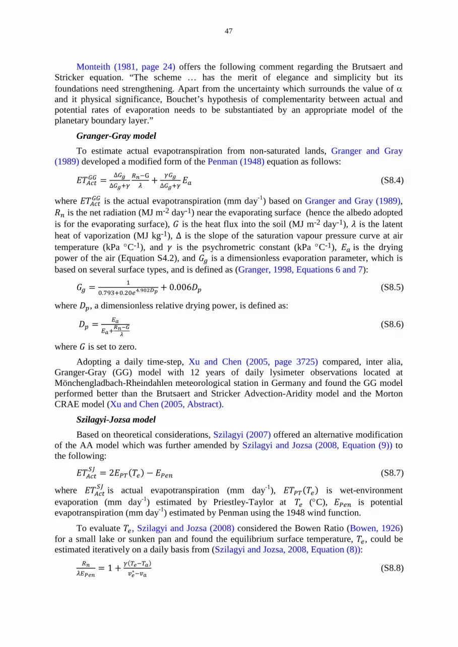
47

Monteith (1981, page 24) offers the following comment regarding the Brutsaert and Stricker equation. “The scheme … has the merit of elegance and simplicity but its foundations need strengthening. Apart from the uncertainty which surrounds the value of α and it physical significance, Bouchet’s hypothesis of complementarity between actual and potential rates of evaporation needs to be substantiated by an appropriate model of the planetary boundary layer.”

Granger-Gray model To estimate actual evapotranspiration from non-saturated lands, Granger and Gray

(1989) developed a modified form of the Penman (1948) equation as follows:

𝐸𝑇𝐴𝑐𝑡𝐺𝐺 = ∆𝐺𝑔∆𝐺𝑔+𝛾

𝑅𝑛−G𝜆

+ 𝛾𝐺𝑔∆𝐺𝑔+𝛾

𝐸𝑎 (S8.4)

where 𝐸𝑇𝐴𝑐𝑡𝐺𝐺 is the actual evapotranspiration (mm day-1) based on Granger and Gray (1989), 𝑅𝑛 is the net radiation (MJ m-2 day-1) near the evaporating surface (hence the albedo adopted is for the evaporating surface), 𝐺 is the heat flux into the soil (MJ m-2 day-1), 𝜆 is the latent heat of vaporization (MJ kg-1), Δ is the slope of the saturation vapour pressure curve at air temperature (kPa °C-1), and 𝛾 is the psychrometric constant (kPa °C-1), 𝐸𝑎 is the drying power of the air (Equation S4.2), and 𝐺𝑔 is a dimensionless evaporation parameter, which is based on several surface types, and is defined as (Granger, 1998, Equations 6 and 7):

𝐺𝑔 = 10.793+0.20𝑒4.902𝐷𝑝 + 0.006𝐷𝑝 (S8.5)

where 𝐷𝑝, a dimensionless relative drying power, is defined as:

𝐷𝑝 = 𝐸𝑎𝐸𝑎+

𝑅𝑛−𝐺𝜆

(S8.6)

where 𝐺 is set to zero. Adopting a daily time-step, Xu and Chen (2005, page 3725) compared, inter alia,

Granger-Gray (GG) model with 12 years of daily lysimeter observations located at Mönchengladbach-Rheindahlen meteorological station in Germany and found the GG model performed better than the Brutsaert and Stricker Advection-Aridity model and the Morton CRAE model (Xu and Chen (2005, Abstract).

Szilagyi-Jozsa model Based on theoretical considerations, Szilagyi (2007) offered an alternative modification

of the AA model which was further amended by Szilagyi and Jozsa (2008, Equation (9)) to the following:

𝐸𝑇𝐴𝑐𝑡𝑆𝐽 = 2𝐸𝑃𝑇(𝑇𝑒) − 𝐸𝑃𝑒𝑛 (S8.7)

where 𝐸𝑇𝐴𝑐𝑡𝑆𝐽 is actual evapotranspiration (mm day-1), 𝐸𝑇𝑃𝑇(𝑇𝑒) is wet-environment

evaporation (mm day-1) estimated by Priestley-Taylor at 𝑇𝑒 (°C), 𝐸𝑃𝑒𝑛 is potential evapotranspiration (mm day-1) estimated by Penman using the 1948 wind function.

To evaluate 𝑇𝑒, Szilagyi and Jozsa (2008) considered the Bowen Ratio (Bowen, 1926) for a small lake or sunken pan and found the equilibrium surface temperature, 𝑇𝑒, could be estimated iteratively on a daily basis from (Szilagyi and Jozsa, 2008, Equation (8)):

𝑅𝑛𝜆𝐸𝑃𝑒𝑛

= 1 + 𝛾(𝑇𝑒−𝑇𝑎)𝑣𝑒∗−𝑣𝑎

(S8.8)

48

where 𝑅𝑛 is the available energy (MJ m-2 day-1), 𝐸𝑃𝑒𝑛 is the Penman evaporation (mm day-1) based on 𝑇𝑎, and 𝑇𝑒 and 𝑇𝑎 are respectively the equilibrium and air temperatures (°C), 𝑣𝑒∗ is the saturation vapour pressure (kPa) at 𝑇𝑒, 𝑣𝑎 is the actual vapour pressure (kPa) at 𝑇𝑎, 𝜆 is the latent heat of vaporization (MJ kg-1), and 𝛾 is the psychrometric constant (kPa °C-1).

Based on daily data and adopting 𝛼𝑃𝑇 = 1.31 but applying the Complementary Relationship to obtain monthly 𝐸𝑇𝐴𝑐𝑡

𝑆𝐽 values, Szilagyi and Jozsa (2008) tested Equation (S8.7) against actual evaporation estimated by Morton’s WREVAP model for 210 SAMSON (Solar and Meteorological Surface Observation Network) stations in the United States and found excellent agreement (R2 = 0.95) (Szilagyi and Jozsa, 2008, Figure 6). Szilagyi et al (2009, page 574) applied their modified AA model to 25 watersheds, 194 SAMSON sites and 53 semi-arid SAMSON sites and concluded that their modified AA model performed better than the Brutsaert and Stricker (1979) traditional AA model.

In applying Equation (S8.7), a daily time-step is used and an albedo value for the vegetative surface is adopted. We note that when we applied Equation (S8.7) to days of very low net radiation, negative values of evaporation were occasionally estimated, a feature also observed in the Brutsaert and Stricker (1979, page 448) Aridity-Advection model (see Section S18).

49

Supplementary Material Section S9 Additional evaporation equations

Although the following empirical equations (except the energy based procedure described at the end of this section) have been extensively referenced or widely used in past practice and therefore are included in this paper, we are of the view that the more physically-based equations described earlier are generally more appropriate for estimating evaporation or evapotranspiration. This is particularly so in regions where empirical coefficients have not been derived.

Dalton-type equations Mass-transfer equations of the following form were first described by John Dalton in

1802 and are known as Dalton-type equations (Dingman, 1992, Section 7.3.2):

𝐸 = 𝐶𝑒𝑚𝑝𝑓(𝑢)(𝑣𝑠∗ − 𝑣𝑎) (S9.1)

where 𝐸 is the actual surface evaporation (mm day-1), 𝑓(𝑢) is an appropriate wind function, 𝑣𝑠∗ is the saturation vapour pressure (kPa) at the evaporating surface, 𝑣𝑎 is the atmospheric vapour pressure (kPa), and 𝐶𝑒𝑚𝑝 is an empirical constant. McJannet et al. (2012) reviewed 19 studies for estimating open water evaporation and proposed a wind function (Equation 14) that depends on the area of the evaporating surface (see Section 2.4.2).

Thornthwaite (1948) In the Thornthwaite evaporation method, the only meteorological data required to

compute mean monthly potential evapotranspiration is mean monthly air temperature, The original steps in Thornthwaite’s (1948) procedure involved a nomogram and tables, which can be represented by the follow equations (Xu and Singh, 2001, Equations 4a and 4b):

𝐸�𝑇ℎ,𝑗 = 16 �ℎ𝑟𝑑𝑎𝑦��

12� �𝑑𝑎𝑦𝑚𝑜𝑛

30� �10𝑇

�𝐽𝐼�𝑎𝑇ℎ

(S9.2)

where 𝐸�𝑇ℎ,𝑗 is the Thornthwaite 1948 estimate of mean monthly potential evapotranspiration (mm month-1) for month 𝑗, (𝑗 = 1 to 12), ℎ𝑟𝑑𝑎𝑦�� is the mean daily daylight hours in month 𝑗, 𝑑𝑎𝑦𝑚𝑜𝑛 is the number of days in month 𝑗, 𝑇�𝐽 is the mean monthly air temperature (oC) in month 𝑗, and 𝐼 is the annual heat index. The annual heat index is estimated as the sum of the monthly indices:

𝐼 = ∑ 𝑖𝑗12𝑗=1 (S9.3)

where 𝑖 = �𝑇�𝐽5�1.514

(S9.4)

and 𝑎𝑇ℎ = 6.75 × 10−7𝐼3 − 7.71 × 10−5𝐼2 + 0.01792𝐼 + 0.49239 (S9.5)

It is noted that strict application of Thornthwaite (1948) yields only 12 values of potential evapotranspiration, a mean value for each calendar month. However, in several studies, Thornthwaite’s procedure has been modified to allow a time series of daily (Federer et al., 1996; Donohue et al., 2010b) or monthly (Xu and Singh, 2001; Lu et al., 2005; Amatya et al., 1995; Xu and Chen, 2005; Trajkovic and Kolakovic, 2009) potential evaporation values to be computed.

Building on Thornthwaite’s (1948) water balance procedure used in his climate classification analysis, Thornthwaite and Mather (1957) developed a procedure for computing a water balance. We suggest readers planning to use the Thornthwaite-Mather method pay

50

attention to Black’s (2007) paper in which he notes that there are significant differences between a 1955 version of the methodology and the 1957 version which, according to Black (2007), is the correct procedure. The Thornthwaite and Mather (1957) methodology consists of applying the 1948 procedure in a water balance context. Scozzafava and Tallini (2001) provide an example.

Makkink model G.F. Makkink, as reported by de Bruin (1981), simplified the Penman (1948) equation

by disregarding the aerodynamic term but compensated the evaporation estimate by introducing two empirical coefficients as follows (Jacobs and de Bruin, 1998, Equation 2):

𝐸𝑀𝑎𝑘 = 𝑐1 �∆

∆+𝛾𝑅𝑠2.45

� − 𝑐2 (S9.6)

where 𝐸𝑀𝑎𝑘 is the Makkink potential evaporation (mm day-1), 𝑅𝑠 is the solar radiation (incoming shortwave) (MJ m-2 day-1) at the water surface, ∆ is the slope of the vapour pressure curve (kPa °C-1) at air temperature, and 𝛾 is the psychrometric constant (kPa °C-1). Adopted values of 𝑐1 and 𝑐2 are 0.61 and 0.12 (mm day-1) (Winter et al., 1995; Xu and Singh, 2002; Rosenberry et al., 2007; Alexandris et al., 2008). According to Rosenberry et al. (2004, Table 1), a monthly time-step is used in the Makkink computations.

FAO-24 Blaney and Criddle (Allen and Pruitt, 1986) There have been a number of modifications made to the original Blaney (1959)

equation for estimating the consumptive use or reference crop evapotranspiration. We outline here the Reference Crop FAO-24 (Allen and Pruitt, 1986; Jensen et al, 1990) version of Blaney and Criddle which is for a grass-related crop evapotranspiration. The method is based on several empirical coefficients which were developed from data measured at adequately watered, agricultural lysimeter sites (Allen and Pruitt, 1986), located in the dry western United States where advection effects were strong (Yin and Brook, 1992).

The FAO-24 Reference Crop version of Blaney-Criddle is defined as (Allen and Pruitt, 1986, Equations 1, 2 and 3; Shuttleworth, 1992, Equation 4.2.45):

𝐸𝑇𝐵𝐶 = �0.0043𝑅𝐻𝑚𝑖𝑛 −𝑛𝑁− 1.41� + 𝑏𝑣𝑎𝑟𝑝𝑦(0.46𝑇𝑎 + 8.13) (S9.7)

𝑏𝑣𝑎𝑟 = 𝑒0 + 𝑒1𝑅𝐻𝑚𝑖𝑛 + 𝑒2𝑛𝑁

+ 𝑒3u2 + 𝑒4𝑅𝐻𝑚𝑖𝑛𝑛𝑁

+ 𝑒5𝑅𝐻𝑚𝑖𝑛u2 (S9.8)

where 𝐸𝑇𝐵𝐶 is the Blaney-Criddle Reference Crop evapotranspiration (mm day-1), 𝑅𝐻𝑚𝑖𝑛 is the minimum relative daily humidity (%), n/N is the measured sunshine hours divided by the possible daily sunshine hours, 𝑝𝑦 is the percentage of actual daytime hours for the day compared to the day-light hours for the entire year, 𝑇𝑎 is the average daily air temperature (oC), and u2 is average daily wind speed (m s-1) at 2 m. The recommended values of the coefficients are from Frevert et al. (1983, Table 1) as follows: 𝑒0 = 0.81917, 𝑒1 = -0.0040922, 𝑒2 = 1.0705, 𝑒3 = 0.065649, 𝑒4= -0.0059684, 𝑒5 = -0.0005967. Due to lower minimum daily temperatures at higher elevation (McVicar et al., 2007 Figure 3), Allen and Pruitt (1986) incorporate an adjustment for elevation to the FAO-24 Blaney-Criddle equation for arid and semi-arid regions following Allen and Brockway (1983) as follows:

𝐸𝑇𝐵𝐶𝐻 = 𝐸𝑇𝐵𝐶 �1 + 0.1 𝐸𝑙𝑒𝑣1000

� (S9.9)

51

where 𝐸𝑇𝐵𝐶𝐻 is the Blaney-Criddle Reference Crop evapotranspiration adjusted for site elevation and 𝐸𝑙𝑒𝑣 is the elevation of the site above mean sea level (m).

Doorenbos and Pruitt (1992, page 4) note that the BC procedure should be used “with scepticism” in equatorial regions (where air temperatures are “relatively constant”), for small islands and coastal areas (where air temperature is affected by sea temperature), for high elevations (due to environmental lapse rate induced low mean daily air temperature) and in monsoonal and mid–latitude regions (with a wide variety of sunshine hours).

It is noted that the original Blaney-Criddle procedure incorporates only monthly temperature data. Consequently, the coefficients 𝑒0, …, 𝑒5 and the climate variables 𝑅𝐻𝑚𝑖𝑛, , 𝑇𝑎, 𝑢2 in Equations (S9.7) and (S9.8), which were based on the crop consumptive use in western United States using the original BC model, will not represent potential evaporation in regions with climates differing from those in western United States. This may explain the Doorenbos and Pruitt (1992) comment in the previous paragraph.

Although the BC method has been used at both a daily and a monthly time-step (Allen and Pruitt, 1986), a monthly period is recommended (Doorenbos and Pruitt, 1992, page 4; Nandagiri and Kovoor, 2006, page 240).

Turc (1961) The Turc method (Turc 1961) is one of the simplest empirical equations used to

estimate reference crop evapotranspiration under humid conditions. (Note that the Turc (1961) equations are very different to those proposed in Turc (1954, 1955).) The Turc 1961 equation, based on daily data, is quoted by Trajković and Stojnić (2007, Equation 1) as:

𝐸𝑇𝑇𝑢𝑟𝑐 = 0.013(23.88𝑅𝑠 + 50) � 𝑇𝑎𝑇𝑎+15

� (S9.10)

where 𝐸𝑇𝑇𝑢𝑟𝑐 is the reference crop evapotranspiration (mm day-1), 𝑇𝑎 is the average air temperature (oC), and 𝑅𝑠 is the incoming solar radiation (MJ m-2 day-1).

For non-humid conditions (RH < 50%), the adjustment provided by Alexandris et al. (2008, Equation 5b) may be used.

𝐸𝑇𝑇𝑢𝑟𝑐 = 0.013(23.88𝑅𝑠 + 50) � 𝑇𝑎𝑇𝑎+15

� �1 + 50−𝑅𝐻70

� (S9.11)

where 𝑅𝐻 is the relative humidity (%).

Because Jensen et al. (1990) identified that the Turc (1961) method performs satisfactorily in humid regions (see Table 5), Trajković and Kolaković (2009) developed an empirical factor to adjust 𝐸𝑇𝑇𝑢𝑟𝑐 for wind speed. Details are given in Trajković and Kolaković (2009).

Hargreaves-Samani (Hargreaves and Samani, 1985) The Hargreaves-Samani equation (Hargreaves and Samani, 1985, Equations 1 and 2),

which estimates reference crop evapotranspiration, is as follows:

𝐸𝑇𝐻𝑆 = 0.0135𝐶𝐻𝑆𝑅𝑎𝜆

(𝑇𝑚𝑎𝑥 − 𝑇𝑚𝑖𝑛)0.5(𝑇𝑎 + 17.8) (S9.12)

where 𝐸𝑇𝐻𝑆 is the reference crop evapotranspiration (mm day-1), 𝐶𝐻𝑆 is an empirical coefficient, 𝑅𝑎 is the extraterrestrial radiation (MJ m-2 day-1), 𝑇𝑚𝑎𝑥, 𝑇𝑚𝑖𝑛, 𝑇𝑎 are respectively the maximum, minimum and average daily air temperature (oC). Samani (2000, Equation 3) proposed a modification to the empirical coefficient to reduce the error associated with the estimation of solar radiation as follows:

52

𝐶𝐻𝑆 = 0.00185(𝑇𝑚𝑎𝑥 − 𝑇𝑚𝑖𝑛)2 − 0.0433(𝑇𝑚𝑎𝑥 − 𝑇𝑚𝑖𝑛) + 0.4023 (S9.13) According to Amatya et al. (1995, Table 4), weekly or monthly data should be used in

the Hargreaves-Samani model in the computation of reference crop evapotranspiration rates.

Modified Hargreaves The modified Hargreaves procedure (Droogers and Allen, 2002), as adapted by Adam

et al (2006, Equation 6), allows one to estimate the reference crop evapotranspiration without wind data using monthly values of rainfall, air temperature, daily air temperature range, and extra-terrestrial solar radiation as follows:

𝐸𝑇𝐻𝑎𝑟𝑔,𝑗 = 0.0013𝑆𝑂�𝑇𝑗 + 17.0��𝑇𝐷��𝑗 − 0.0123𝑃𝑗�0.76

(S9.14)

where, for a given month j, 𝐸𝑇𝐻𝑎𝑟𝑔,𝑗 is the modified Hargreaves monthly reference crop evapotranspiration (mm day-1), 𝑇𝑗 is the monthly mean daily air temperature (°C), 𝑇𝐷��𝑗 is the mean monthly difference between mean daily maximum air temperature and mean daily minimum air temperature (°C) for month j, 𝑃𝑗 is the monthly precipitation (mm month-1), and S0 is the mean monthly water equivalent for extraterrestrial solar radiation (mm day-1). If 𝑇𝐷��𝑗 data are unavailable, New et al. (2002) have provided 10′ latitude/longitude gridded mean monthly diurnal air temperature range. Again, following the approach of Adam et al. (2006, Equations 7, 8, 9 and 10), S0 is estimated by:

𝑆0 = 15.392𝑑𝑟2�𝜔𝑠𝑠𝑖𝑛(𝑙𝑎𝑡)𝑠𝑖𝑛(𝛿) + 𝑐𝑜𝑠(𝑙𝑎𝑡)𝑐𝑜𝑠(𝛿)𝑠𝑖𝑛(𝜔𝑠)� (S9.15)

where 𝑙𝑎𝑡 is the latitude of the location in radians (negative for southern hemisphere), dr is the relative distance between the earth and the sun, given by:

𝑑𝑟2 = 1 + 0.033𝑐𝑜𝑠 � 2π365

𝐷𝑜𝑌� (S9.16)

where 𝐷𝑜𝑌 is the Day of Year (see Section S3), ωs is the sunset hour angle in radians (see Adam et al., 2006, page 22 for boundary conditions) and is given by:

𝜔𝑠 = 𝑎𝑟𝑐𝑜𝑠(−𝑡𝑎𝑛(𝑙𝑎𝑡)tan (𝛿)) (S9.17)

and δ is the solar declination in radians given by:

δ = 0.4093𝑠𝑖𝑛 � 2𝜋365

𝐷𝑜𝑌 − 1.405� (S9.18)

Evapotranspiration estimates are based on a monthly time-step.

Application based on energy balance A very different approach to the application of energy balance is by McLeod and

Webster (1996, Equations 8 and 9) who used data from an instrumented irrigation channel to estimate channel evaporation from:

𝐸𝑖𝑐 = (𝑅𝑛+𝑄𝑣−𝑄𝑡)

�1+𝐵+𝑐𝑤𝑇𝑠λ �

∆𝑡λ

(S9.19)

where 𝐸𝑖𝑐 is the evaporation from the irrigation channel (mm day-1), 𝑅𝑛 is the net radiation on the water surface (MJ m-2 day-1), 𝑄𝑣 is the heat flux advected into the water body (MJ m-2 day-1), 𝑄𝑡 is the heat flux increase in stored energy (MJ m-2 day-1), 𝐵 is the Bowen Ratio, 𝑐𝑤 is specific heat of water (MJ kg-1 °C-1), 𝑇𝑠 is the temperature of the evaporated water (°C), ∆𝑡 is time interval over which the fluxes are estimated (day), and λ is the latent heat of vaporisation (MJ kg-1).

53

Supplementary Material Section S10 Estimating deep lake evaporation

Based on a review of the literature, Table S5 provides guidelines to define deep and shallow lakes for the purpose of estimating lake evaporation. (The background to Table S5 is discussed in the Section S11.)

Kohler and Parmele (1967)

The Penman estimate of open-water evaporation, 𝐸𝑃𝑒𝑛𝑂𝑊, (Equation (12)) is a starting point to estimate evaporation from a deep lake using the Kohler and Parmele (1967) procedure. To account for water advected energy and heat storage, Kohler and Parmele (1967, Equation 12) recommended the following relationship:

𝐸𝐷𝐿 = 𝐸𝑃𝑒𝑛𝑂𝑊 + 𝛼𝐾𝑃(𝐴𝑤 −∆𝑄∆𝑡

) (S10.1)

where 𝐸𝐷𝐿 is the evaporation from the deep lake (mm day-1), 𝐸𝑃𝑒𝑛𝑂𝑊 is the Penman open-water evaporation (mm day-1), 𝛼𝐾𝑃 is the proportion of the net addition of energy from advection and storage used in evaporation during ∆𝑡, 𝐴𝑤 is the net water advected energy during ∆𝑡 (mm day-1), and ∆𝑄

∆𝑡 is the change in stored energy (mm day-1). Kohler and Parmele

(1967, page 1002) illustrated their method adopting ∆𝑡 = 1 day. The three other terms are complex and following Dingman (1992, Equations 7.38, 7.31 and 7.32 respectively) can be computed from:

𝛼𝐾𝑃 = ∆

∆+𝛾+4𝜀𝑤𝜎(𝑇𝑤+273.2)3

𝜌𝑤λ𝐾𝐸𝑢 (S10.2)

𝐴𝑤 = 𝑐𝑤𝜌𝑤 𝜆

(𝑃𝑑𝑇𝑝 + 𝑆𝑊𝑖𝑛𝑇𝑠𝑤𝑖𝑛 − 𝑆𝑊𝑜𝑢𝑡𝑇𝑠𝑤𝑜𝑢𝑡 + 𝐺𝑊𝑖𝑛𝑇𝑔𝑤𝑖𝑛 − 𝐺𝑊𝑜𝑢𝑡𝑇𝑔𝑤𝑜𝑢𝑡) (S10.3)

∆𝑄 = 𝑐𝑤𝜌𝑤𝐴𝐿𝜆

(𝑉2𝑇𝐿2 − 𝑉1𝑇𝐿1) (S10.4)

where ∆ is the slope of the vapour pressure curve (kPa °C-1) at air temperature, 𝜀𝑤 is the effective emissivity of the water (dimensionless), 𝜎 is the Stefan-Boltzman constant (MJ m-2 day-1 K-4), 𝑇𝑤 is the temperature of the water (°C), 𝑇𝑝 is the temperature of precipitation (°C), 𝑐𝑤 is the specific heat of water (MJ kg-1 °C-1), 𝑃𝑑 is the precipitation rate (mm day-1), λ is the latent heat of vaporization (MJ kg-1), 𝐾𝐸 is a coefficient that represents the efficiency of the vertical transport of water vapour (kPa-1), 𝑢 is mean daily wind speed (m day-1), SW and GW represent surface and ground water inflows and outflows as per subscript (mm day-1) and V’s and T’s represent respective average lake volumes (m3) and temperatures (°C), 𝐴𝐿 is lake area (m2), and 1 and 2 identify values at the beginning and end of ∆𝑡. Generally, for surface lakes GW will be small with respect to SW and can be ignored, but for a deep void following surface mining, groundwater may need to be assessed. Estimation of 𝐾𝐸 (m day2 kg-1) is based on Equation (S10.5), but may need to be adjusted for atmospheric stability (see Dingman, 1992, Equation 7.2):

𝐾𝐸 = 0.622 𝜌𝑎𝑝𝜌𝑤

1

6.25�𝑙𝑛�𝑧𝑚−𝑧𝑑𝑧0

��2 (S10.5)

where 𝜌𝑎 is the density of air (kg m-3), 𝜌𝑤 is the density of water (kg m-3), 𝑝 is the atmospheric pressure (kPa), 𝑧𝑚 is the height above ground level (m) at which the wind speed

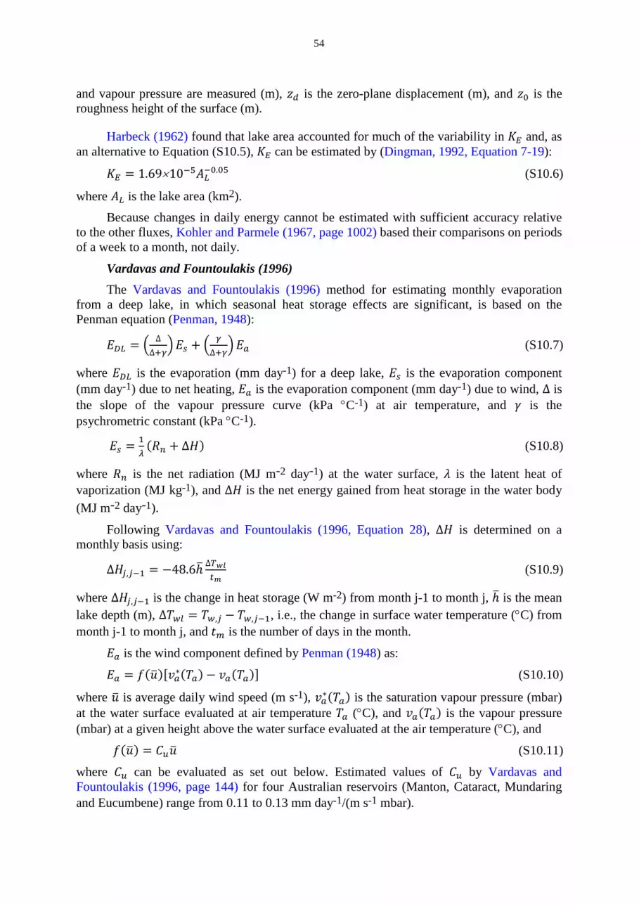
54

and vapour pressure are measured (m), 𝑧𝑑 is the zero-plane displacement (m), and 𝑧0 is the roughness height of the surface (m).

Harbeck (1962) found that lake area accounted for much of the variability in 𝐾𝐸 and, as an alternative to Equation (S10.5), 𝐾𝐸 can be estimated by (Dingman, 1992, Equation 7-19):

𝐾𝐸 = 1.69×10−5𝐴𝐿−0.05 (S10.6)

where 𝐴𝐿 is the lake area (km2). Because changes in daily energy cannot be estimated with sufficient accuracy relative

to the other fluxes, Kohler and Parmele (1967, page 1002) based their comparisons on periods of a week to a month, not daily.

Vardavas and Fountoulakis (1996) The Vardavas and Fountoulakis (1996) method for estimating monthly evaporation

from a deep lake, in which seasonal heat storage effects are significant, is based on the Penman equation (Penman, 1948):

𝐸𝐷𝐿 = � ∆∆+𝛾

�𝐸𝑠 + � 𝛾∆+𝛾

�𝐸𝑎 (S10.7)

where 𝐸𝐷𝐿 is the evaporation (mm day-1) for a deep lake, 𝐸𝑠 is the evaporation component (mm day-1) due to net heating, 𝐸𝑎 is the evaporation component (mm day-1) due to wind, ∆ is the slope of the vapour pressure curve (kPa °C-1) at air temperature, and 𝛾 is the psychrometric constant (kPa °C-1).

𝐸𝑠 = 1𝜆

(𝑅𝑛 + Δ𝐻) (S10.8)

where 𝑅𝑛 is the net radiation (MJ m-2 day-1) at the water surface, 𝜆 is the latent heat of vaporization (MJ kg-1), and Δ𝐻 is the net energy gained from heat storage in the water body (MJ m-2 day-1).

Following Vardavas and Fountoulakis (1996, Equation 28), Δ𝐻 is determined on a monthly basis using:

∆𝐻𝑗,𝑗−1 = −48.6ℎ� ∆𝑇𝑤𝑙𝑡𝑚

(S10.9)

where ∆𝐻𝑗,𝑗−1 is the change in heat storage (W m-2) from month j-1 to month j, ℎ� is the mean lake depth (m), ∆𝑇𝑤𝑙 = 𝑇𝑤,𝑗 − 𝑇𝑤,𝑗−1, i.e., the change in surface water temperature (°C) from month j-1 to month j, and 𝑡𝑚 is the number of days in the month.

𝐸𝑎 is the wind component defined by Penman (1948) as:

𝐸𝑎 = 𝑓(𝑢�)[𝑣𝑎∗(𝑇𝑎) − 𝑣𝑎(𝑇𝑎)] (S10.10)

where 𝑢� is average daily wind speed (m s-1), 𝑣𝑎∗(𝑇𝑎) is the saturation vapour pressure (mbar) at the water surface evaluated at air temperature 𝑇𝑎 (°C), and 𝑣𝑎(𝑇𝑎) is the vapour pressure (mbar) at a given height above the water surface evaluated at the air temperature (°C), and

𝑓(𝑢�) = 𝐶𝑢𝑢� (S10.11)

where 𝐶𝑢 can be evaluated as set out below. Estimated values of 𝐶𝑢 by Vardavas and Fountoulakis (1996, page 144) for four Australian reservoirs (Manton, Cataract, Mundaring and Eucumbene) range from 0.11 to 0.13 mm day-1/(m s-1 mbar).

55

Following Vardavas (1987, Equation 23) 𝐶𝑢 can be evaluated from:

𝐶𝑢 = 3966

𝑇𝑎𝑙𝑛�𝑧2𝑧𝑜𝑣

�𝑙𝑛� 𝑧1𝑧𝑜𝑚

� (S10.12)

where 𝑇𝑎 is the air temperature (K), 𝑧1 is the height above ground of the wind speed measurement (m), 𝑧2 is the height above ground of the water vapour measurement (m). 𝑧𝑜𝑚, the momentum roughness (m), and 𝑧𝑜𝑣, the roughness length for water vapour (m), are given by:

𝑧𝑜𝑚 = 0.135 υ𝑢∗

(S10.13)

𝑧𝑜𝑣 = 0.624 υ𝑢∗

(S10.14)

where υ is the kinematic viscosity of air (m2 s-1) and is estimated by:

υ = 2.964×10−7 𝑇𝑎3/2

𝑝 (S10.15)

where 𝑇𝑎 is the air temperature (K), and 𝑝 is the atmospheric pressure (kPa).

The friction velocity, 𝑢∗, is computed from:

𝑢� = 𝑢∗𝑘𝑙𝑛 � 𝑧2𝑢∗

0.135υ� (S10.16)

where 𝑘 is von Kármán’s constant, 𝑢� is the mean wind speed (m s-1), 𝑧2 is the height above ground of water vapour measurement (m), and υ is the kinematic viscosity of air (m2 s-1). 𝑢∗ can be estimated by a numerical iteration technique, e.g., Newton-Raphson.

Other approaches that may be appropriate Several approaches that have been included under Section S11 Estimating shallow lake

evaporation may be appropriate for deep lakes. In particular, McJannet et al. (2008b) procedure has been tested for two deep lakes.

56

Supplementary Material Section S11 Estimating shallow lake evaporation

Based on a review of the literature, Table S5 provides guidelines to define deep and shallow lakes for the purpose of estimating lake evaporation. According to Monteith (1981, page 9), it is inappropriate to apply the Penman equation to estimating evaporation from open water bodies that exceed “… a metre or so in depth…” because of the damping due to heat stored in the water. Morton’s (1986) analysis indicates “… the CRLE model has little advantage over the CRWE at depths less than 1.5 m”. For shallow lakes of 3 m mean depth, de Bruin (1978) and Sacks et al (1994) consider it unnecessary to take account of seasonal heat storage in estimating lake evaporation, whereas Fennessey (2000), in his study of a shallow lake of 2 m mean depth, incorporated monthly heat storage. For a shallow lake (average depth of 0.6 m and characterised by a bottom crust of a thick frozen mud layer) in Hudson Bay, Canada, Stewart and Rouse (1976) incorporated heat flux through the bottom of the lake and the heat capacity of the water.

Based on the above evidence we suggest as a general guide that seasonal heat storage be taken into account for shallow lakes with an average water depth of 2 m or more. For shallow lakes with water depth less than 2 m, we prefer the Penman equation (Equation (12)) with the 1956 wind function..

Shallow lake evaporation by Penman equation based on the equilibrium temperature (Finch, 2001)

To take heat storage into account, Finch (2001) used the concept of equilibrium temperature and tested the accuracy of the method by estimating evaporation from a shallow lake. A description of the model is presented by Keijman (1974) and de Bruin (1982). As noted in Section (2.1.4), the equilibrium temperature is the temperature of the surface water when the net rate of heat exchange at the water surface is zero (Edinger et al., 1968, page 1139). In this context, Sweers (1976, page 377) assumes that, although on clear calm days a water body will exhibit strong temperature gradients near the water surface, the top 0.5 m – 1.0 m or so is well mixed and its mean temperature specifies the surface temperature.

To estimate shallow lake evaporation, Finch (2001) adopted Penman (1948) but incorporated the Sweers (1976, Equation 18) wind function (Equation (S11.2)) and the equilibrium temperature. In the method it is assumed the water column is well mixed and the heat flux at the bed of the water body can be neglected (Finch, 2001, pages 2772). For each daily time-step, the following nine equations are computed:

𝜆𝐸 = ∆(𝑅𝑛𝑤−𝐺𝑤)+𝛾𝜆𝑓(𝑢)(𝑣𝑎∗−𝑣𝑎)(∆+𝛾) (S11.1)

𝜆𝑓(𝑢) = 0.864(4.4 + 1.82𝑢) (S11.2)

where 𝐸 is daily lake evaporation (mm day-1), 𝑅𝑛𝑤 is the net daily radiation (MJ m-2 day-1) based on the surface water temperature, 𝐺𝑤 is the daily change in heat storage (MJ m-2 day-

1), 𝜆 is the latent heat of vaporisation (MJ kg-1), (𝑣𝑎∗ − 𝑣𝑎) is the vapour pressure deficit (kPa) at air temperature, 𝛾 is psychrometric constant (kPa K-1), ∆ is the slope of the saturation vapour curve (kPa K-1) at air temperature, and 𝑢 is the mean daily wind speed (m s-1) at 10 m. (Note that many wind measuring instruments are at a height of 2 m rather than 10 m and for those situations the wind speed needs to be adjusted by Equation (S4.4).)

However, before 𝑅𝑛𝑤 and 𝐺𝑤 can be estimated the daily surface water temperature of the lake needs to be estimated as follows:

57

𝑇𝑤,𝑖 = 𝑇𝑒 + �𝑇𝑤,𝑖−1 − 𝑇𝑒�𝑒1𝜏 (S11.3)

where 𝑇𝑤,𝑖, 𝑇𝑤,𝑖−1 are the surface water temperatures (°C) on day 𝑖 and day 𝑖 − 1 respectively, and 𝑇𝑒 is the equilibrium temperature (°C) and 𝜏 is equilibrium temperature time constant (days). 𝑇𝑒 and 𝜏 are estimated as follows:

𝑇𝑒 = 𝑇𝑤𝑏 + 𝑅𝑤𝑏∗

4𝜎(𝑇𝑤𝑏+273.1)3+𝜆𝑓(𝑢)(Δwb+𝛾) (Finch, 2001, page 2773) (S11.4)

where 𝑅𝑤𝑏∗ is the net radiation (MJ m-2 day-1) based on wet-bulb temperature (𝑇𝑤𝑏) (°C) and is estimated by:

𝑅𝑤𝑏∗ = (1 − 𝛼)𝑅𝑠 + 𝑅𝑖𝑙 − 𝐶𝑓[𝜎(𝑇𝑎 + 273.1)4 + 4𝜎(𝑇𝑎 + 273.1)3(𝑇𝑤𝑏 − 𝑇𝑎)] (S11.5)

𝜏 = 𝜌𝑤𝑐𝑤ℎ𝑤4𝜎(𝑇𝑤𝑏+273.1)3+𝜆𝑓(𝑢)(Δwb+𝛾) (Finch, 2001, page 2772) (S11.6)

where 𝜏 is the equilibrium temperature time constant (days), 𝑇𝑤𝑏 is the mean daily wet-bulb temperature (°C), 𝑅𝑠 is the shortwave solar radiation (MJ m-2 day-1), 𝛼 is the albedo for a water surface (Finch (2001) estimated using Payne (1972)), 𝑅𝑖𝑙 is incoming longwave radiation (MJ m-2 day-1), 𝐶𝑓 is a cloudiness factor, 𝜎 is the Stefan-Boltzman constant (MJ m-

2 K-4 day-1), 𝑇𝑎 is mean daily air temperature (°C) at screen height, Δwb is the slope of the saturation vapour curve (kPa K-1) at wet-bulb temperature, 𝛾 is the psychrometric constant (kPa K-1), 𝜌𝑤 is the density of water (kg m-3), 𝑐𝑤 is the specific heat of water (MJ m-2 K-4 day-

1), and ℎ𝑤 is the depth of the lake (m).

Thus, having an estimate of the surface water temperatures from Equation (S11.3), 𝑅𝑛𝑤 and 𝐺𝑤 are estimated from:

𝑅𝑛𝑤 = (1 − 𝛼)𝑅𝑠 + 𝑅𝑖𝑙 − 𝐶𝑓�𝜎(𝑇𝑎 + 273.1)4 + 4𝜎(𝑇𝑎 + 273.1)3�𝑇𝑤,𝑖−1 − 𝑇𝑎�� (S11.7)

𝐺𝑤 = 𝜌𝑤𝑐𝑤ℎ𝑤�𝑇𝑤,𝑖 − 𝑇𝑤,𝑖−1� (S11.8)

where 𝑅𝑛𝑤 is the net radiation given the surface water temperature, 𝑇𝑤,𝑖, 𝑇𝑤,𝑖−1 are the surface water temperature on day 𝑖 and day 𝑖 − 1 respectively.

Next, 𝜆𝐸 can be estimated using Equation S11.1 and the depth of water ℎ𝑤 on day 𝑖 + 1 is estimated as:

ℎ𝑖+1 = ℎ𝑖 + 𝑃𝑖+1 − 𝐸𝑖 (S11.9)

where 𝑃𝑖+1 is the rainfall measured on day 𝑖 + 1 and 𝐸𝑖 is the lake evaporation on day 𝑖. According to deBruin (1982, page 270) because water bodies up to 10 m deep are

generally well mixed by wind, the model is of practical significance. The meteorological data are assumed to be land-based (Finch, 2001, page 2771) and the model uses a daily time-step.

The model was applied by Finch (2001) to a small reservoir at Kempton Park, UK resulting in the annual evaporation being 6% lower than the measured value.

Shallow lake evaporation by finite difference model (Finch and Gash, 2002) Finch and Gash (2002) proposed a finite difference approach as an alternative to

estimating shallow lake evaporation. The steps are set out as follows (Finch and Gash, 2002, Figure 1):

1. Estimate ∝ (shortwave albedo for the water surface).

58

2. Set the first estimate of 𝑇𝑤 (average water temperature) at the beginning of the current time-step to the value at the end of the previous time-step.

3. Calculate the average 𝑇𝑤. 4. Calculate 𝑅𝑛 (net radiation). 5. Calculate 𝑓(𝑢) (𝑢 is wind speed at a height of 10 m). 6. Calculate 𝜆𝐸 (latent heat flux) and 𝐻 (sensible heat flux). 7. Calculate 𝑊(change in heat storage in water column during the current time-step). 8. Calculate a new estimate of 𝑇𝑤 at the end of the time-step. 9. Is the difference between the last estimate of 𝑇𝑤 and the present one < 0.01? 10. If no, return to step 3, otherwise proceed to the next time-step.

The equations to estimate the above variables are as follows (Finch and Gash, 2002):

∝ = 𝑓(𝑔,𝜃 ) (S11.10)

𝑔 = 𝑅𝑠𝑆𝑐𝑜𝑛 𝑠𝑖𝑛𝜃

𝑑𝑟2

1 (S11.11)

𝑇𝑤 = 𝑇𝑤,𝑖−1 + �𝑇𝑤,𝑖−𝑇𝑤,𝑖−12

� (S11.12)

𝑅𝑛𝑤 = 𝑅𝑠(1 − 𝛼) + 𝑅𝑖𝑙 − 𝐶𝑓𝜎(𝑇𝑤 + 273.1)4 (S11.13)

𝑓(𝑢) = 0.216𝑢Δ+𝛾

for 𝑇𝑤 ≤ 𝑇𝑎 (S11.14)

𝑓(𝑢) =0.216𝑢�1+10(𝑇𝑤−𝑇𝑎)

𝑢2�0.5

Δ+𝛾 for 𝑇𝑤 > 𝑇𝑎 (S11.15)

𝜆𝐸 = 𝑓(𝑢)(𝑣𝑤∗ − 𝑣𝑑) (S11.16)

𝐻 = 𝛾𝑓(𝑢)(𝑇𝑤 − 𝑇𝑎) (S11.17)

∆𝑊 = 𝑅𝑛 − 𝜆𝐸 − 𝐻 (S11.18)

𝑇𝑤,𝑖 = 𝑇𝑤,𝑖−1 + ∆𝑊𝜌𝑤𝑐𝑤ℎ𝑤

(S11.19)

where 𝛼 is shortwave albedo for the water surface, 𝑅𝑠 is the incoming shortwave radiation (MJ m-2 d-1), 𝑆𝑐𝑜𝑛 is the solar constant = 0.0820 MJ m-2 day-1, 𝜃 is the Sun’s altitude (°), 𝑑𝑟 is the ratio of the actual to mean Earth-Sun separation or the inverse relative distance Earth-Sun, 𝑇𝑤 is average water temperature (°C), 𝑇𝑤,𝑖 and 𝑇𝑤,𝑖−1 are, respectively, the estimated water temperature (°C) at the end of the current and previous periods, 𝑇𝑎 is the air temperature (°C) at the reference height, 𝑅𝑛𝑤 is the net radiation (MJ m-2 d-1), 𝑅𝑖𝑙 is incoming longwave radiation (MJ m-2 day-1) , 𝐶𝑓 is a cloudiness factor, 𝜎 is the Stefan-Boltzman constant (MJ m-2 K-4 day-1), Δ is the slope of the saturation vapour pressure curve at air temperature (kPa K-1), 𝛾 is the psychrometric constant (kPa K-1), 𝑢 is wind speed (m s-1) at a height of 10 m, 𝑣𝑤∗ is the saturation vapour pressure at the water temperature (kPa), 𝑣𝑑 is the vapour pressure at the reference height (kPa), 𝜆𝐸 is the latent heat flux (MJ m-2 d-1), 𝐻 is the sensible heat flux (MJ m-2 d-1), ∆𝑊 is change in heat storage in water column during the current time-step (MJ m-2 d-

1), 𝜌𝑤 is the density of water (kg m-3), 𝑐𝑤 is the specific heat of water, and ℎ𝑤 is the depth of water (m).

1 In Equation (S11.11), we have adopted Payne’s equation (Payne, 1972, Equation 3; see also Berger et al, 1993, Equation 2) and Simpson and Paulson (1979, Equation 2) in which 𝑑𝑟2 is used rather than 𝑑𝑟 as published in the Finch and Gash (2002) paper.

59

𝑅𝑠 is either measured solar radiation or estimated from Equation S3.9 and 𝑅𝑖𝑙 may be estimated from Equation (S3.16). Finch and Gash (2002) used Payne (1972, Table 1) to estimate ∝ knowing 𝑔 and 𝜃. 𝑔 requires 𝑑 to be estimated which is computed from:

𝑑𝑟2 = 1 + 0.033𝑐𝑜𝑠 � 2𝜋365

𝐷𝑜𝑌� (S11.20)

where 𝐷𝑜𝑌 is day of year (𝐷𝑜𝑌 = 1, 2, …, 365).

𝜃 is estimated as follows (Al-Rawi, 1991, Equation 1):

sin𝜃 = cos (𝑙𝑎𝑡) cos (𝛿) cos (𝜔𝑠) + sin (𝑙𝑎𝑡) sin (𝛿) (S11.21)

where 𝑙𝑎𝑡 is latitude in radians, 𝛿 is the solar declination angle in radians, and 𝜔𝑠 is the sunset hour angle in radians. 𝛿 and 𝜔𝑠 can be estimated from Equations (S9.18) and (S9.17) respectively.

Lake evaporation by Penman-Monteith equation based on the equilibrium temperature (McJannet et al., 2008b)

McJannet et al. (2008b) adopted the Penman-Monteith as the basis of applying the equilibrium temperature to estimate lake evaporation for a range of water bodies – shallow and deep lakes and an irrigation canal. Their approach is similar to that used by Finch (2001). We reproduce below the method proposed and tested by McJannet et al. (2008b). Evaporation is estimated as follows:

𝐸𝑀𝑐𝐽 = 1𝜆�𝛥𝑤(𝑄∗−𝐺𝑤)+86400𝜌𝑎𝑐𝑎�𝑣𝑤

∗ −𝑣𝑎�𝑟𝑎

𝛥𝑤+𝛾� (S11.22)

where 𝐸𝑀𝑐𝐽 is the evaporation from the water body (mm day-1), 𝑄∗ is the net radiation (MJ m-

2 day-1), 𝐺𝑤 is the change in heat storage in the water body (MJ m-2 day-1), 𝜌𝑎 is the density of air (kg m-3), 𝑐𝑎 is the specific heat of air (MJ kg-1 K-1), 𝑣𝑤∗ is the saturation vapour pressure at water temperature (kPa), 𝑣𝑎 is the daily vapour pressure (kPa) taken at 9:00 am, 𝜆 is the latent heat of vaporisation (MJ kg-1), 𝛥𝑤 is the slope of the saturation water vapour curve at water temperature (kPa °C-1), 𝛾 is the psychrometric constant (kPa °C-1), and 𝑟𝑎 is the aerodynamic resistance (s m-1) and is defined by Calder and Neal (1984, page 93) and McJannet et al. (2008b, Appendix B, Equation 10) as:

𝑟𝑎 = 𝜌𝑎𝑐𝑎𝛾� 𝑓(𝑢)

86400� (S11.23)

where from Sweers (1976, page 398) and modified by McJannet et al. (2008b, Appendix B, Equation 11) and converting units from W m-2 mbar-1 to MJ m-2 kPa-1 day-1 yields:

𝑓(𝑢) = �5𝐴�0.05

(3.80 + 1.57𝑢10) (S11.24)

where 𝑢10 is the wind speed (m s-1) at 10 m and 𝐴 (km2) is the area of the water body, and other variables are defined previously. (For elongated water bodies, the square of the width was adopted as the area (Sweers, 1976, page 398).)

𝑄∗ in Equation (S11.22) is defined as:

𝑄∗ = 𝑅𝑠(1 − 𝛼) + (𝑅𝑖𝑙 − 𝑅𝑜𝑙) (S11.25)

where 𝑅𝑠 is the total daily incoming shortwave radiation (MJ m-2 day-1), 𝛼 is albedo for water (= 0.08), 𝑅𝑖𝑙 is the incoming longwave radiation (MJ m-2 day-1), and 𝑅𝑜𝑙 is the outgoing longwave radiation (MJ m-2 day-1).

60

𝑅𝑖𝑙 = �𝐶𝑓 + �1 − 𝐶𝑓� �1 − �0.261 𝑒𝑥𝑝(−7.77 × 10−4𝑇𝑎2)��𝜎(𝑇𝑎 + 273.15)4 (S11.26)

where 𝐶𝑓 is the fraction of cloud cover, 𝑇𝑎 is the mean daily air temperature (°C), and 𝜎 is the Stefan-Boltzmann constant (MJ m-2 K-4 day-1).

𝑅𝑜𝑙 = 0.97 𝜎(𝑇𝑤 + 273.15)4 (S11.27)

where 𝑇𝑤 is the water temperature (°C) which will vary for each time-step and must be estimated before Equation (S11.22) can be applied.

Because the heat storage in a water body affects surface water temperatures and, therefore, evaporation, it is necessary to predict heat storage changes over time which depend on the equilibrium temperature (𝑇𝑒), the time constant for the storage (𝜏), as well as the water temperature (𝑇𝑤). Equilibrium temperature is the surface temperature at which the net rate of heat exchange is zero (see Section 2.1.4). Again, following McJannet et al. (2008b, Equation 23), we estimate water temperature, based on de Bruin (1982, Equation 10), from the following equation:

𝑇𝑤 = 𝑇𝑒 + (𝑇𝑤0 − 𝑇𝑒)exp �− 1𝜏� (S11.28)

where 𝑇𝑤0 is the water temperature (°C) in the previous time-step, 𝑇𝑒 is the equilibrium temperature (°C), and 𝜏 is the time constant (day).

Following McJannet et al. (2008b, Equation 5), the time constant (𝜏) in days is given by (de Bruin, 1982, Equation 4):

𝜏 = 𝜌𝑤𝑐𝑤ℎ𝑤4𝜎(𝑇𝑤𝑏+273.15)3+𝑓(𝑢)(Δwb+𝛾) (S11.29)

where 𝜌𝑤 is the density of water (kg m-3), 𝑐𝑤 is the specific heat of water (MJ kg-1 K-1), ℎ𝑤 is the water depth (m), 𝛥𝑤𝑏 is the slope of the saturation water vapour curve (kPa °C-1) estimated at wet-bulb temperature (𝑇𝑛) (°C). The water depth ℎ𝑤 could be a time-series if required (see Equation (S11.9).

The equilibrium temperature is estimated from (de Bruin, 1982, Equation 3):

𝑇𝑒 = 𝑇𝑤𝑏 + 𝑄𝑤𝑏∗

4𝜎(𝑇𝑤𝑏+273.15)3+𝑓(𝑢)(Δwb+𝛾) (S11.30)

where 𝑄𝑤𝑏∗ is the net radiation at wet-bulb temperature and is estimated by:

𝑄𝑤𝑏∗ = 𝑅𝑠(1 − 𝛼) + �𝑅𝑖𝑙 − 𝑅𝑜𝑙𝑤𝑏� (S11.31)

and where 𝑅𝑜𝑙𝑤𝑏 is the outgoing longwave radiation (MJ m-2 day-1) at wet-bulb temperature and is estimated as follows:

𝑅𝑜𝑙𝑤𝑏 = 𝜎(𝑇𝑎 + 273.15)4 + 4𝜎(𝑇𝑎 + 273.15)3(𝑇𝑤𝑏 − 𝑇𝑎) (S11.32)

The change in heat storage, Gw, is calculated from (McJannet et al. (2008b, Equation 31):

𝐺𝑤 = 𝜌𝑤𝑐𝑤ℎ𝑤(𝑇𝑤 − 𝑇𝑤0) (S11.33)

Thus, for the time-step in question, 𝑇𝑤 and 𝐺𝑤 are now known and 𝐸𝑀𝑐𝐽 in Equation (S11.22) can be computed.

The McJannet et al. (2008b) model operates at a daily time-step.

61

Based on the above approach, McJannet et al. (2008b) applied gridded climate data to estimate average daily (and monthly) evaporation for a range of water bodies from an irrigation canal to five large lakes. Overall, the modelled estimates are within 10% of the independent evaporation estimates (McJannet et al., 2008b, Section 5.7), however, the correlation coefficient between monthly modelled and observed evaporation values is very low for two of the lake studies.

A worked example is provided in Section S19.

The differences between Finch (2001) and McJannet et al. (2008b) procedures to estimate lake evaporation are:

Finch (2001) McJannet et al. (2008b)

Adopted Penman (1948) equation Adopted Penman-Monteith equation

Wind function depends on wind speed Wind function depends on wind speed and lake area

Adjusted water level for daily rainfall and daily evaporation loss

No adjustment of water level for rainfall or evaporation

Tested on one 10 m lake in UK Tested on three shallows lakes, a weir, an irrigation channel and two deep reservoirs

Lake evaporation by lake-specific vertical temperature profiles

Sometimes for a lake, monthly or seasonal vertical water temperature profiles are available that can be used to estimate the vertical water body heat flux (𝐺𝑤 in Equations (S11.1) and (11.22)). Fennessey (2000) provides an example for a shallow lake in Massachusetts, U.S as follows:

𝐺𝑤 is defined more precisely as a function of time

𝐺𝑤(𝑡) = 𝑑𝐻(𝑡)𝑑𝑡

(S11.34)

where 𝐻(𝑡) is the total heat energy content of the lake per unit area of the lake surface at time 𝑡 (MJ m-2) and is computed by:

𝐻(𝑡) = 𝜌𝑤𝑐𝑤𝐴𝑠

∑ �𝑇𝑤(𝑧𝑖+1)+𝑇𝑤(𝑧𝑖)2

�𝑚𝑖=1 𝑉𝑖 (S11.35)

where the lake is segregated into 𝑚 horizontal layers, each layer being (𝑧𝑖+1 − 𝑧𝑖) thick (m) , 𝜌𝑤 is the density of water (kg m-3), 𝑐𝑤 is the specific heat of water (MJ kg-1 K-1), 𝐴𝑠 is the surface area of the lake (m2), 𝑇𝑤(𝑧𝑖) and 𝑇𝑤(𝑧𝑖+1) are respectively the water temperature at 𝑧𝑖 and 𝑧𝑖+1, and 𝑉𝑖 is the volume (m3) of each layer defined by:

𝑉𝑖 = (𝐴𝑖+1+𝐴𝑖)(𝑧𝑖+1−𝑧𝑖)2

(S11.36)

Thus, 𝐺𝑤(𝑡) can be incorporated in the Penman based equation of Finch (2001) (Equation S11.1) or in the Penman-Monteith based equation of McJannet et al. (2008b) (Equation S11.22).

62

Supplementary Material Section S12 Estimating evaporation from lakes covered by vegetation

Brezny et al. (1973, Table 1) measured the evaporation rate of cattail, Typha augustfolia L., in 0.36 m2 tanks in Rajashan, India. Over approximately 75 days, they found that the evaporation from tanks with plants was 52% more than the evaporation from tanks without plants. In contrast, based on a comparison of measured evaporation from Barren Box Swamp (a lake covered with cattail, Typha orientalis PRESL., in NSW, Australia) compared with a lake devoid of vegetation, Linacre et al. (1970, Table IV) observed over three days 34% less evaporation from the swamp compared to a nearby lake without vegetation. Linacre et al. (1970, page 385) attributed the lower observed evaporation from swamp compared with the lake evaporation to lower albedo of the clear water in the lake, to the shelter provided by the reeds in the swamp, and to the internal resistance to water movement of the reeds. These contrasting results illustrate the difficulty in assessing the impact of vegetation on evaporation from lakes.

There is an extensive body of literature addressing the question of evaporation from lakes covered by vegetation. Abtew and Obeysekera (1995) summarise the results of 19 experiments which, overall, show that the transpiration of macrophytes is greater than open surface water. However, most experiments were not carried out in situ. On the other hand, Mohamed et al. (2008) lists the results of 11 in situ studies (estimating evaporation by eddy correlation or Bowen Ratio procedures) in which wetland evaporation is overall less than open surface water.

Based on theoretical considerations and a literature survey, Idso (1981) offered the following observations. Firstly, reliable experiments assessing the relative rates of evaporation from vegetated water bodies and open surface water must be conducted in situ (Idso (1981, page 46). Secondly, for extensive water bodies covered by vegetation, evaporation will most likely be lower than the open surface water estimate (Idso (1981, page 47). It is noted that Anderson and Idso (1987, page 1041) concluded that canopy surface geometry is important in the evaporative process and, therefore, for small or narrow canopies (e.g., macrophytes along stream reaches where advective energy is significant), evaporative water losses greater than open water can occur.

Drexler et al. (2004, page 2072) in a review of models and methods to estimate wetland evapotranspiration offered the following comments.

1. For many wetland types, the physical processes are poorly characterised. 2. Generalisation is difficult because of variable nature of the results, even within

well-studied vegetation types. 3. The wetland environment is very varied, making it particularly difficult to measure

ET. 4. Seasonal variation of ET is also an important consideration.

A number of models – Penman (Section S4), Penman-Monteith (Section S5), the Shuttleworth-Wallace variation of Penman-Monteith (Section S5), and Priestley-Taylor (Section 2.1.3) – have been used in several studies (Wessel and Rouse, 1994; Abtew and Obeysekera, 1995; Souch et al. 1998; Bidlake, 2000; Lott and Hunt, 2001; Jacobs et al., 2002; Drexler et al., 2004) to estimate the rate of evaporation from a lake covered by vegetation. Table S7 summarises seven comparisons and suggests that the weighted Penman-Monteith method which is able to account for variations of 𝑟𝑎 and 𝑟𝑠 for different vegetation surface

63

performs satisfactorily. For this model, and based on one experiment, the mean model estimate of lake evaporation compared to a mean measured value was 1.10.

Readers are referred to a very recent review by Clulow et al (2012) in which they discuss, inter alia, under what conditions Penman, Priestley-Taylor and Penman-Monteith models can be used to estimate actual evaporation from a lake covered by vegetation.

64

Supplementary Material Section S13 Estimating potential evaporation in rainfall-runoff

modelling Several procedures including Penman-Monteith, Priestley-Taylor and Morton have

been used in daily and monthly rainfall-runoff modelling at a daily or monthly time-step to estimate potential evaporation/evapotranspiration. In the Penman-Monteith model the aerodynamic and surface roughness coefficients (𝑟𝑎 and 𝑟𝑠 respectively) need to be specified in Equation (5). Some typical values of 𝑟𝑎 and 𝑟𝑠 are listed in Table S2. In a sensitivity analysis in which the Penman-Monteith equation was incorporated into the SHE model (Abbott et al., 1986a, b), Beven (1979, page 176 and Figure 5) adopted constant values of 𝑟𝑎 = 46 s m-1 for grass and 4 s m-1 for pine forest. However, values varied from mid-day (𝑟𝑠 = 50 s m-1 for grass and 100 s m-1 for pine forest) to mid-night ( 𝑟𝑠 = 200 s m-1 for grass and 400 s m-1 for pine forest). Beven concluded that the evapotranspiration estimates were very dependent on the values of the aerodynamic and canopy resistance parameters.

In using the Priestley-Taylor algorithm (Equation (6)) for estimating catchment potential evapotranspiration, the parameter 𝛼𝑃𝑇 needs to be specified. Zhang et al (2001, Equation 4) adopted 1.28 and Raupach et al. (2001, page 1152) recommended 1.26. It should be noted that the 𝛼𝑃𝑇 ‘constant’ is commonly set to 1.26 although optimised values vary greatly depending on the moisture and advective conditions in which the measurements are made (see Table S8). This is not surprising as the Priestley-Taylor algorithm was developed assuming non-advective conditions and without recourse to measurement of the aerodynamic component.

One of the advantages of Morton’s (1983a) CRAE method to estimate potential evapotranspiration is that it does not require wind data as input and, therefore, has been used extensively in Australia to estimate historical monthly potential evapotranspiration in rainfall-runoff modelling (Chiew and Jayasuria, 1990; Chiew and McMahon, 1993; Chiew et al., 1993; Jones et al., 1993; Siriwardena et al., 2006). In many water engineering applications, analysis depends on measured or estimated monthly runoff and potential evaporation over an extended period, often more than 100 years.

There are at least two options available to analysts to estimate Morton’s 𝐸𝑇𝑊𝑒𝑡 in Australia. One approach is to use the mean monthly areal potential values (equivalent to wet environment areal evapotranspiration using Morton’s nomenclature) produced jointly by the CRC for Catchment Hydrology and the Bureau of Meteorology in 2001 (see http://www.bom.gov.au/climate/averages and Wang et al. (2001) with detailed methodology described in Chiew et al. (2002)). For daily modelling, the mean monthly values can be disaggregated into equal daily values. A major disadvantage with this approach is that there is no variation in potential evapotranspiration from year to year. However, Chapman (2003, Section 5) applied four rainfall-runoff models to 15 catchments in Australia and concluded that, in terms of modelling daily streamflow, equally good results could be obtained by using average monthly potential evapotranspiration data in the place of daily potential evapotranspiration values. Rather than adopting average monthly values, Oudin et al. (2005) used average daily values in an application of four rainfall-runoff models to 308 catchments in Australia, France and the United States. They concluded that the average daily potential evaporation values resulted in modelled runoffs that were little different to those produced using daily varying potential evaporation (Oudin et al., 2005, Tables 3 and 4).

http://www.bom.gov.au/climate/averages

65

The second option is to estimate Morton’s wet environmental evapotranspiration from climate data using Equation (18). Chiew and Jayasuria (1990) reviewed Morton’s wet environmental evapotranspiration and compared, for three locations in south-eastern Australia, daily estimates of Morton’s wet environmental evapotranspiration with Penman’s free-water evaporation. They concluded that (i) Morton’s model can estimate successfully daily global and net radiation (Chiew and Jayasuria, 1990, page 293); (ii) Morton’s wet environment evaporation can be used to represent potential evapotranspiration in rainfall-runoff modelling (Chiew and Jayasuria, 1990, page 293); (It should be noted that this assessment was based on Penman rather than the more appropriate Penman-Monteith model.) (iii) Morton’s 𝐸𝑇𝑊𝑒𝑡 cannot estimate low potential evapotranspiration values accurately and underestimates high values (Chiew and Jayasuria, 1990, page 291).

Based on data for 19 climate stations in Australia from 1970 to 1989, Chapman (2001) demonstrated that overall pan evaporation data are a better estimate of potential evapotranspiration than maximum air temperature. Furthermore, he developed the following simple relationship (applicable only to Australia) that could be used if no other data were available to estimate potential evaporation for catchment modelling purposes:

𝐸𝑇𝑒𝑞𝑃𝑀 = 𝐴𝑝𝐸𝑃𝑎𝑛 + 𝐵𝑝 (S13.1)

where 𝐸𝑇𝑒𝑞𝑃𝑀 is the daily equivalent Penman-Monteith potential evaporation (mm day-1), 𝐸𝑃𝑎𝑛 is the daily Class-A pan evaporation (mm day-1), and 𝐴𝑝 and 𝐵𝑝 are given by:

𝐴𝑝 = 0.17 + 0.011𝐿𝑎𝑡 (S13.2)

𝐵𝑝 = 10(0.66−0.211 𝐿𝑎𝑡) (S13.3)

where 𝐿𝑎𝑡 is the latitude of the catchment in degrees South.

66

Supplementary Material Section S14 Estimating evaporation of intercepted rainfall

It is recognised that interception is variable in space and in time. According to Klaassen et al. (1998) the interception storage of water in dense forests is an important process and varies seasonally (Gerrits et al., 2010) and across vegetation types. Crockford and Richardson (2000) note that because interception is dependent on rainfall and other meteorological variables it is difficult to make conclusions about interception losses for specific vegetation types.

Because potential evaporation rates are higher in the hotter months of a year and lower during colder months, interception is seasonal. Other factors such as rainfall intensity, wind, and snow also impact interception storage and, hence, interception evaporation (Gerrits et al., 2010). Gerrits et al. (2010) note that although interception storage can be very variable; for the beech forest they studied in Luxembourg, its size played a minor role in evaporation. Stewart (1977) has shown that the evaporation of transpired water is very different to the evaporation of intercepted water and, hence, it is important that these two components are considered separately.

Although Herbst et al. (2008) state that the Gash model (Gash, 1979) is the most widely and successfully used interception model, Gerrits et al. (2010) adopted the Rutter model (Rutter et al., 1971, 1975) in their analysis. In his model, Gash (1979) incorporated the Penman-Monteith equation which was found by Herbst et al. (2008) to give estimates of wet canopy evaporation equivalent to those estimates from the eddy covariance energy balance approach. In the 1971 Rutter model the authors (Rutter et al., 1971) incorporated the Penman (1956) equation to estimate potential evaporation.

Teklehaimanot and Jarvis (1991) concluded from their experiments that evaporation rates from a wet canopy could be satisfactorily modelled by the Penman (1948) equation. Moreover, they further showed that the actual evaporation from a partially wet canopy could be modelled by multiplying the Penman evaporation by 𝐶𝑟𝑒𝑡/𝑆𝑐𝑎𝑛 , where 𝐶𝑟𝑒𝑡 is the amount of water retained on the canopy (mm) and 𝑆𝑐𝑎𝑛 is the storage capacity of the canopy (mm).

An issue of double counting can arise when evaporation of rainfall interception from the canopy is estimated independently from transpiration. The impact of double counting according to Gash and Stewart (1975) can be an over-estimation of interception evaporation by about 7% (see also Miralles et al., 2011).

Readers are referred to a recent and comprehensive review by Muzylo et al. (2009), who addressed the theoretical basis of 15 interception models including their evaporation components, who identified inadequacies and research questions, and who noted there were few comparative studies and little information about uncertainty in measured and modelled parameters.

Modelling evapotranspiration-interception in an urban area Grimmond and Oke (1991) developed a hydrologic model of an urban area at an hourly

time-step to estimate evaporation over a range of meteorological conditions. The model includes the Penman (1948) equation modified by Monteith (1965) for vegetation surface and the Rutter et al. (1971) interception model modified by Shuttleworth (1978) to provide a smooth transition between wet and dry vegetation canopies. In addition, anthropogenic heat flux and stored heat flux were also modelled. The model was tested for a small urban area in Vancouver, Canada and according to the authors the model showed promise.

68

Supplementary Material Section S15 Estimating bare soil evaporation

Following Philip (1957), Ritchie (1972, page 1205) proposed a two-stage model to estimate bare soil evaporation. Salvucci (1997) developed further the Ritchie approach defining the evaporation loss for stage-1 by:

𝐸𝑠𝑡𝑎𝑔𝑒 1 = 𝐸�𝑃𝑒𝑛𝑚𝑎𝑛× 𝑡1 (S15.1)

where 𝐸𝑠𝑡𝑎𝑔𝑒 1 is the cumulative stage-1 bare soil evaporation (mm) which, according to Allen et al. (1998, page 145), should not exceed the readily evaporable water (REW) which they define as the maximum depth of water that can be evaporated from the top-soil without restriction. Typical REW values are: sand 2 – 7 mm, loam 8 – 10 mm and clay 8 – 12 mm. 𝑡1 is the length of the stage-1 atmosphere-controlled evaporation period (day) which is defined as:

𝑡1 = 𝑅𝐸𝑊𝐸�𝑃𝑒𝑛𝑚𝑎𝑛

(S15.2)

𝐸�𝑃𝑒𝑛𝑚𝑎𝑛 is the daily average stage-1 actual evaporation (mm day-1) and is assumed to be at or near the rate of Penman evaporation. McVicar et al. (2012, page 183) prefers to use the term energy-limited rather than stage-1. Alternatively, a more rigorous procedure to estimate 𝑡1 is recommended by Dingman (1992, page 293) who suggests the end of stage-1 is readily observed from ground or satellite observations of albedo.

Discussing evaporation from bare soil, Monteith (1981, pages 10 and 11) observes that “When bare soil is thoroughly wetted, the soil surface behaves like water in so far as the relative humidity of the air in contact with the surface is 100%”. Monteith (1981, page 11) further adds that as a matter of observation the rate of evaporation “…is usually very close to the rate for adjacent short vegetation, despite differences in radiative and aerodynamic properties”.

Stage-2 evaporation (the water-limited stage, McVicar et al. (2012, page 183)), is dependent on stage-1 and two limiting cases need to be considered.

1. Where the unsaturated hydraulic conductivity (mm day-1), 𝐾𝑢𝑠 << 𝐸�𝑃𝑒𝑛𝑚𝑎𝑛. This would occur with relatively low permeability soils.

2. Where 𝐾𝑢𝑠 >> 𝐸�𝑃𝑒𝑛𝑚𝑎𝑛 and, therefore, the cumulative drainage is much greater than the cumulative actual evaporation.

Salvucci (1997, Equations 18 and 19 respectively) developed the following empirical equations for the two cases:

For 𝐾𝑢𝑠 << 𝐸�𝑃𝑒𝑛𝑚𝑎𝑛

𝐸𝑏𝑠𝑜𝑖𝑙(𝑡) = 𝐸𝑠𝑡𝑎𝑔𝑒 1 �−0.621 + 1.621 � 𝑡𝑡1��0.5

, 𝑡 ≥ 𝑡1 (S15.3)

For 𝐾𝑢𝑠 >> 𝐸�𝑃𝑒𝑛𝑚𝑎𝑛

𝐸𝑏𝑠𝑜𝑖𝑙(𝑡) = 𝐸𝑠𝑡𝑎𝑔𝑒 1 �1 + 0.811𝑙𝑛 � 𝑡𝑡1��, 𝑡 ≥ 𝑡1 (S15.4)

where 𝐸𝑏𝑠𝑜𝑖𝑙(𝑡) is the cumulative bare soil evaporation up to time t. As a check on the total evaporable water (TEW), typical values for a range of soils are

provided by Allen et al. (1998, Table 19). For example, sand = 6 – 12 mm, loam = 16 – 22 mm and clay = 22 – 29 mm. TEW is defined by Allen et al. (1998, Equation 73) as:

69

𝑇𝐸𝑊 = 10(𝜃𝐹𝐶 − 0.5𝜃𝑊𝑃)𝑧𝑒 (S15.5)

where 𝜃𝐹𝐶 is the soil moisture content (%) at field capacity, 𝜃𝑊𝑃 is the soil moisture content (%) at wilting point, 𝑧𝑒 is the depth of the surface soil layer that is subject to drying from evaporation. If this is unknown, Allen et al. (1998, page 144) recommend 𝑧𝑒 = 0.10 – 0.15 m.

It is interesting to note that Penman (1948, page 137) observed from his experiments that freshly wetted bare soil evaporated at about 90% of the rate observed for open surface water for the same weather conditions.

Based on FAO56 methodology (Allen et al., 1998), Allen et al. (2005) developed a two-stage strategy (energy limited and water limited stages) to estimate bare soil evaporation. Mutziger et al (2005) applied the methodology to seven data sets and concluded that model accuracy was about ±15%.

70

Supplementary Material Section S16 Class-A pan evaporation equations and pan coefficients

Although some researchers, e.g., Watts and Hancock (1984, page 295), are critical of an evaporative pan as a reliable climatic instrument (they list 10 potential problems), it should be noted that Roderick et al. (2009b, Section 4) comment “…that the pan evaporation record provides the only direct measurement of changing evaporative demand…” which is crucial in climate change studies. In Australia, 60 stations have been identified as high quality Class-A pan evaporation stations (Jovanovic et al., 2008).

Equations: Kohler et al. (1955) Kohler et al. (1955) (see Dingman (1992, Equation 7.41)) developed the following

empirical equations to estimate daily open-water evaporation, 𝐸𝑓𝑤 (mm day-1) from Class-A pan evaporation data:

𝐸𝑓𝑤 = 0.7[𝐸𝑃𝑎𝑛 + 0.064𝑝𝛼𝑃𝑎𝑛(0.37 + 0.00255𝑢𝑃𝑎𝑛)|𝑇𝑃𝑎𝑛 − 𝑇𝑎|0.88] for 𝑇𝑃𝑎𝑛 > 𝑇𝑎

(S16.1)

𝐸𝑓𝑤 = 0.7[𝐸𝑃𝑎𝑛 − 0.064𝑝𝛼𝑃𝑎𝑛(0.37 + 0.00255𝑢𝑃𝑎𝑛)|𝑇𝑃𝑎𝑛 − 𝑇𝑎|0.88] for 𝑇𝑃𝑎𝑛 < 𝑇𝑎

(S16.2)

where 𝐸𝑃𝑎𝑛 is the daily evaporation measured by an unguarded Class-A pan (mm day-1), p is the atmospheric pressure (kPa), 𝛼𝑃𝑎𝑛 is the proportion of energy exchanged through the sides of the pan and is specified in Equation (S16.3), 𝑢𝑃𝑎𝑛 is the average daily wind speed at a height of 150 mm above the pan (km day-1), and 𝑇𝑝𝑎𝑛 and 𝑇𝑎 are respectively the mean daily pan water and air temperature (°C).

𝛼𝑃𝑎𝑛 = 0.34 + 0.0117𝑇𝑃𝑎𝑛 − 3.5×10−7(𝑇𝑃𝑎𝑛 + 17.8)3 + 0.00135𝑢𝑃𝑎𝑛0.36 (S16.3)

Wind run for anemometers not at 150 mm above the pan should be adjusted using Equation (S4.4). Based on an intercontinental comparison, Burman (1976) concluded that the Kohler et al. (1955) equations were superior to empirical methods proposed by Christiansen (1968) and Oliver (1961) which are not included here.

Equations: Chiew & McMahon (1992) Chiew and McMahon (1992, Appendix) developed daily, 3-day, weekly and monthly

pan coefficients as simple linear regressions of the form:

𝐸𝑃𝑒𝑛,𝑗 = 𝐼𝑗 + 𝐺𝑗𝐸𝑃𝑎𝑛,𝑗 (S16.4)

where for month j, 𝐸𝑃𝑒𝑛,𝑗 is the Penman (1948) estimate of evaporation for a land environment rather than open water, 𝐸𝑃𝑎𝑛,𝑗 is the evaporation from a Class-A pan, and 𝐼𝑗 and 𝐺𝑗 are respectively the intercepts and the gradients of daily, 3-day, weekly and monthly totals. Values of 𝐼𝑗 and 𝐺𝑗 for 26 climate stations in Australia are given in Chiew and McMahon (1992).

Equations: Allen et al (1998)

Equations for estimating Reference Crop evapotranspiration, 𝐸𝑅𝐶, are presented by Allen et al. (1998, page 55, Table 7) taking into account the site of the pan in terms of the upwind fetch as follows:

𝐸𝑇𝑅𝐶 = 𝐾𝑃𝑎𝑛𝐸𝑃𝑎𝑛 (S16.5)

71

where 𝐾𝑃𝑎𝑛 is the pan coefficient given by: for a green vegetated fetch (1 to 1000 m) within a dry area at least 50 m wide

𝐾𝑃𝑎𝑛 = 0.108 − 0.0286𝑢2 + 0.0422𝑙𝑛(𝐹𝐸𝑇) + 0.1434𝑙𝑛(𝑅𝐻𝑚𝑒𝑎𝑛)− 0.000631[𝑙𝑛(𝐹𝐸𝑇)]2𝑙𝑛(𝑅𝐻𝑚𝑒𝑎𝑛)

(S16.6)

for a dry fetch (1 to 1000 m) within a green vegetated area at least 50 m wide

𝐾𝑃𝑎𝑛 = 0.61 + 0.00341𝑅𝐻𝑚𝑒𝑎𝑛 − 0.000162𝑢2𝑅𝐻𝑚𝑒𝑎𝑛 − 0.00000050𝑢2𝐹𝐸𝑇+ 0.00327𝑢2𝑙𝑛(𝐹𝐸𝑇) − 0.00289𝑢2𝑙𝑛(86.4𝑢2)− 0.0106𝑙𝑛(86.4𝑢2)𝑙𝑛(𝐹𝐸𝑇) + 0′00063[𝑙𝑛(𝐹𝐸𝑇)]2𝑙𝑛(86.4𝑢2)

(S16.7)

where 𝐹𝐸𝑇 is the fetch or length of the identified surface (m), 𝑢2 is the daily wind speed at 2 m height, and 𝑅𝐻𝑚𝑒𝑎𝑛 is the mean daily relative humidity (%). According to Allen et al. (1998, Table 7), Equations (S16.6) and (S16.7) should not be used outside the following ranges 1 m ≤ FET ≤ 1000 m, 30% ≤ 𝑅𝐻𝑚𝑒𝑎𝑛 ≤ 84%, and 1 ms-1 ≤ 𝑢2 ≤ 8 m s-1.

A range of pan coefficients based on Equations (S16.6) and (S16.7) are displayed in Table S9 which illustrates the importance of appropriately specifying the microclimate around a pan in order to have a representative estimate of Reference Crop evapotranspiration. Because 𝐸𝑃𝑎𝑛 = 𝐸𝑇𝑅𝐶

𝑓𝑃𝑎𝑛, we are able to use the table to explore how the evaporating power (in

this case being represented by pan evaporation 𝐸𝑃𝑎𝑛) is affected quantitatively by the characteristics of a site. For example, the pan evaporation under a light wind, low humidity and a green vegetated fetch will be reduced by ~14% for a 10 m fetch compared with a 1000 m one; for a dry fetch under the same conditions, the pan evaporation will increase by ~20%.

Equations: Snyder et al. (2005) Based on pan data in California, Snyder et al. (2005, Equations 6, 8 and 9) proposed the

following set of empirical equations to estimate reference crop evaporation.

𝐸𝑇𝑅𝐶 = 10𝑠𝑖𝑛 ��𝐸𝑝𝑎19.2

� 𝜋2� (S16.8)

𝐸𝑝𝑎 = 𝐸𝑝𝑎𝑛𝐹100 (S16.9)

𝐹100 = −0.0035[𝑙𝑛(𝐹)]2 + 0.0622[𝑙𝑛(𝐹)] + 0.79 (S16.10)

where 𝐸𝑇𝑅𝐶 is the reference crop evapotranspiration (mm day-1), 𝐸𝑝𝑎𝑛 is the Class-A pan evaporation (unscreened) (mm day-1) and 𝐹 is the upwind grass fetch (m). The method is suitable for semi-arid conditions but would require calibration for humid or windier climates (Snyder et al., 2005, page 252).

Ghare et al. (2006) introduced modifications to the Snyder equations but field testing in Italy and Serbia by Trajkovic and Kolakovic (2010) showed that the original Snyder model performed better.

Computed monthly and annual Class-A pan coefficients Although it is not possible to check independently that pan coefficients are correct, one

can compare computed values with those found in the literature. Published results of estimating the pan coefficients for the two Penman wind functions (Equations S4.5 and S4.6) are presented in Table S10 along with pan coefficients for Reference Crop evapotranspiration

72

and the Priestley-Taylor potential evaporation. The exceptionally low pan coefficients for Priestley-Taylor are based on 16 climate stations in Jordon. The coefficients are plotted against mean annual unscreened Class-A pan evaporation in Figure S2 which illustrates, at least for this arid environment, that adopting a spatially constant pan coefficient may be unwise. This observation is consistent with McVicar et al. (2007, Figure 10) who observed for the Coarse Sandy Hill catchments in north-central China both spatial and seasonal variations in pan coefficients.

Published monthly and annual open-water pan coefficients are often extrapolated to other locations. Care needs to be taken as several local factors will impact pan coefficients including relative humidity (Alvarez et al., 2007; Hoy and Stephens, 1979; Kohler et al., 1955), reservoir dimensions (Alvarez et al., 2007), degree of stratification (Hoy and Stephens, 1979), presence of aquatic plants (Winter, 1981), and lake turbidity and salinity (Grayson et al., 1996). Locally calibrated coefficients are preferred.

Australian pan coefficients In Australia, in order to prevent the consumption of water by birds and animals, bird

guards (wire screens) were installed progressively on the Class-A evaporation pans during the late 1960s and early 1970s, and by 1975 most pans were operating with screens which reduce the evaporation. van Dijk (1985) compared the evaporation recorded from evaporation pans with and without bird guards at four Australian locations between 1967 to 1971. The average monthly effect at the four locations ranged from 4.1% to 8.2% reduction in measured evaporation, with an average of 6.6%. These reductions are less than the values of 13% for humid areas and 10% for semi-arid regions noted in a review by Lincare (1994). Based on the findings of van Dijk (1985), the Australian Bureau of Meteorology (2007) recommends an annual conversion factor of +7%. Jovanovic et al. (2008) have developed a high-quality monthly pan evaporation data set that includes 60 locations across Australia covering the period from about 1970 to present for monitoring evaporation trends.

In Australia, the associated climate data required to estimate open-water evaporation (𝐸𝑓𝑤) (mm/unit time) using Equation (S16.1) or (S16.2) are not available at many pan evaporation sites and, as a consequence, monthly (or annual) pan coefficients are developed using:

𝐸𝑓𝑤,𝑗 = 𝐾𝑗𝐸𝑃𝑎𝑛,𝑗 (S16.11)

where j is the specific month and 𝐾𝑗 is the average monthly pan coefficient. Traditionally, 𝐾𝑗 is assumed constant, although Linacre (1994, Figure 1) using Stanhill’s (1976) data for 12 sites world-wide found that for very high evaporation rates 𝐾𝑗 decreased from the nominal 0.7 value.

Hoy and Stephens (1977; 1979) calculated the monthly pan coefficients of seven Australian reservoirs by comparing the evaporation of a Class-A pan with the heat budget method over several years. The average monthly pan estimates are listed in Table S11. Annual pan coefficients were estimated for a greater number of Australian reservoirs by Hoy and Stephens (1977; 1979) and these results are listed in Table S12.

We have computed monthly pan coefficients for 68 sites across Australia by correlating monthly evaporation values from Class-A evaporation pans with corresponding Penman evaporation estimates using his 1956 wind function, based on measured daily climate data at the same or a nearby location, thus yielding open-water evaporation. Thirty-nine of the 68 sites are part of the high quality evaporation pan network (Jovanovic et al., 2008, Table 1);

73

another 29 stations with monthly pan coefficients have been included in the analysis for spatial completeness. Pan coefficients are presented in Table S6. At least 10 monthly values are used in calculating 79.4% of the computed monthly pan coefficients. The analysis of the results in the table shows that mean monthly pan coefficients (weighted for length of record) across the 68 Australian stations is 0.80. This average value compares with 0.76 (based on published data in Table S10 for Penman (1956) and Penman (1948) the latter adjusted by Equation (S4.8) to be equivalent to Penman (1956)). It should be noted that in computing the monthly solar radiation term in the Penman model, the coefficients 𝑎𝑠 and 𝑏𝑠 in Equation (S3.9) were optimised to 0.05 and 0.65 respectively (Section S6).

For many practical problems, annual evaporation estimates need to be disaggregated into monthly values or monthly evaporation values into daily values. This process is not straightforward, when there is no concurrent at-site climate data which could be used to provide guidance as to how the annual or monthly values should be partitioned.

For annual evaporation, a standard approach is to use monthly pan coefficients if available. Another approach, that is available to Australian analysts, is to apply the average monthly values of point potential evapotranspiration for the given location and pro rata the values to sum to the annual evaporation. Maps for each calendar month are available in Wang et al. (2001). This approach is based on the recent analysis by Kirono et al. (2009, Figure 3) who found that, for 28 locations around Australia, Morton’s potential evapotranspiration 𝐸𝑇𝑃𝑜𝑡 correlated satisfactorily (R2 = 0.81) with monthly Class-A pan evaporation although over-estimating pan evaporation by 8%.

For monthly disaggregation to daily data in Australia one could utilize the analysis of Rayner (2005) who reports on synthetic gridded daily Class-A pan evaporation data based on solar radiation and vapour pressure deficit (Jeffrey et al., 2001). The grids are at a spatial resolution of 0.05°(~5 km) and cover the period 1919 to present. McVicar et al. (2007, page 211) note, however, that if pan coefficients are spatially averaged across a range of climates the averaged value will tend to be damped.

Modifying pan data for estimating evaporation from a deep lake To estimate deep lake evaporation from pan data, Webb (1966, Equation 3) proposed an

alternative approach based on vapour pressure to estimate monthly lake evaporation by summing daily values as follows:

𝐸𝐿,𝑑 = 1.50 𝑣𝐿∗−𝑣4

𝑣𝑃∗−𝑣4

𝐸′𝑝𝑎𝑛 (S16.12)

where 𝐸𝐿,𝑑 is the daily estimate of lake evaporation (mm day-1), 𝐸′𝑝𝑎𝑛 is the daily pan evaporation (mm day-1), 𝑣𝐿∗ is the afternoon average lake saturation vapour pressure (mbar), 𝑣𝑃∗ is the afternoon maximum pan saturation vapour pressure (mbar), and 𝑣4 is the afternoon average vapour pressure 4 m above the ground surface (mbar). The monthly evaporation value is the sum of the daily values. The empirical coefficient of 1.50 was established from Lake Hefner data.

74

Supplementary Material Section S17 Comparing published evaporation estimates

A detailed review of the literature identified 27 papers in which comparisons were made between model estimates of potential or actual evaporation or evapotranspiration and field measurements (water balance studies, Bowen Ratio or eddy correlation), lysimeter observation or comparisons between evaporation equations. Detailed discussion of field measurements of evaporation are outside the scope of this paper. We refer readers to Harbeck (1958), Grant (1975), Myrup et al. (1979), Brutsaert (1982), Dingman (1992, Sections 7.8.2 and 7.8.3), Lenters et al. (2005), and Ali et al. (2008) for applications of the techniques. Details for each of the 27 studies are listed Table 5. For each study two items of information are generally provided in the table – the ratio of the average model values (daily, monthly or annual) to a base value, and a measure of error generally as a root mean square error or standard error of estimate. For four studies, multiple sets of results are available.

The bias results (ratios in Table 5) are consolidated in Table 6 under six headings. Under the first two headings each model result is compared with measured observations. For the six lake studies a water balance, eddy correlation or Bowen Ratio estimate were the basis of the comparison. For the seven non-lake studies, the base estimates were from eddy correlation or Bowen Ratio experiments. The third comparison of four studies is based on lysimeter observations. The remaining three sets of comparisons are between various models and Penman-Monteith, Priestley-Taylor or Hargreaves-Samani estimates. The results are summarised in Figure 3 where each model ratio value includes at least two studies.

In interpreting these results, readers should note the comment of Winter and Rosenberry (1995, page 983) who stated that “Regardless of their intended use, it is not uncommon for equations developed for determination of potential evapotranspiration from vegetation to be used for determination of evaporation from open water”.

The information in Figure 3 requires some interpretation. Firstly, the ratios in column (1) “Lakes”, column (2) “Lysimeter” and column (3) “Land” may be regarded as absolute estimates in the sense that the modelled estimates are compared against measured evaporation. Secondly, ratios in columns (4) “Relative to PM” and (5) “Relative to PT” are relative to Penman-Monteith and Priestley-Taylor set to a ratio value of 1.00. Thirdly, the values in columns (1) and (2) are for open-water (“Lakes”) or “Lysimeter” measurements, in which water is not limiting in either comparison. On the other hand, values in column (3) will have been influenced by the availability of soil moisture to the plants and by the vegetation type and, therefore, will not be evaporating or transpiring at a potential rate. This would explain why Turc (Tu) and the Priestley-Taylor (PT) values differ markedly between columns (2) and (3).

Table 5 also contains error information mainly as a root mean square error (RMSE) or as a standard error of estimate (SEE). We have summarised the relevant results in Table 7 which lists the root mean square error (mm day-1) or the standard error of estimate (mm day-

1). Because the values of RMSE or SEE were available for Priestley-Taylor in all comparisons, relative errors (as the ratio of RMSE or SEE for the particular model to that for PT) have been computed. These results are summarised as the median for each method. As a guide, the median RMSE for the six Priestley-Taylor analyses is 0.97 mm day-1 and 0.66 mm day-1 for the eight SEE values.

75

Supplementary Material Section S18 Comparing evaporation estimates based on measured

climate data for six Australian automatic weather stations Table S13 shows the results of estimating annual evaporation for 14 daily and monthly

evaporation/evapotranspiration models based separately on daily and monthly climate data recorded at six widely distributed Australian automatic weather stations over the period January 1979 to March 2010. The latitude and longitude of each station are listed in the table along with the mean annual rainfall estimated for the concurrent period used in the computation of evaporation estimates. Annual values are the sum of 12 monthly means. The number of days and complete months of data available at each station is as follows: Perth Airport (6238 days, 192 months), Darwin Airport (11307 days, 334 months), Alice Springs Airport (11288 days, 320 months), Brisbane Airport (3674 days, 111 months), Melbourne Airport (3842 days, 116 months), and Grove (Companion) (9622 days, 241 months). The authors advise that care needs to be exercised in extending more widely any conclusions arising from this analysis of only six stations.

The results in the table are listed under four main groups: those that estimate actual open-water evaporation (i) Penman 1956 (P56), Priestley-Taylor (PT), Makkink (Ma); (ii) those that estimate reference crop evaporation – FAO-56 Reference Crop (FAO-56 RC), Blaney-Criddle (BC), Hargreaves-Samani (HS), modified Hargreaves (mod H), Turc (Tu); (iii) models that estimate actual evapotranspiration – Morton (Mo), Brutsaert-Stricker (BS), Granger-Gray (GG), Szilagyi-Jozsa SJ); and (iv) three additional methods that include Thornthwaite’s monthly potential estimates (Th), PenPan modelled estimates of actual Class-A pan evaporation (PP), and actual evaporation measured by a Class-A evaporation pan. In interpreting these results readers should note that we have applied each method as set out in the relevant reference except we adopted a time-step of both one day and one month. For some models the recommended time-step for analysis is longer than one day. This information is provided where the model is discussed in the paper.

For the daily data in each group, the ratio of the annual evaporation to the value for a key method is calculated and listed as the “Daily ratio”. Also for each station, the ratio of annual estimates based on monthly and daily data (M to D ratio) are compared. Several observations follow:

1. Relative to the key procedure in each group, the evaporation estimates in Table S13 are reasonably consistent, excepted for Blaney-Criddle, across the six sites which have very different climates. As noted in Section S9 the Blaney-Criddle procedure was developed for application in the dry western United States and, therefore, may not perform successfully in regions subject to a different climate (like Melbourne or Grove) where the procedure appears to perform inadequately. See also item 9 below.

2. On averaging the daily ratios for the open water group, the actual evaporation estimates for Priestley-Taylor and Makkink are 0.88× and 0.59× the Penman 1956 estimate. This is consistent with our summary of published data presented in Table 6 and Figure 3.

3. For the reference crop group, Hargreaves-Samani and Turc are 1.10× and 0.90× the FAO-56 Reference Crop average, again consistent with the lysimeter data listed in Table 6 and Figure 3.

4. The PenPan estimates for the six stations are consistent with the values plotted in Figure S3 which are based on 68 Australian stations.

5. The results in Table S13 show that for Penman 1956, Priestley-Taylor, Makkink, FAO-56 Reference Crop, Turc, Granger-Gray and PenPan there is less than ~2% difference in

76

annual evaporation estimates using a daily or a monthly time-step. However, for Szilagyi-Jozsa and Brutsaert-Stricker, the monthly values are respectively 7% and 10% higher than the daily values whereas for Hargreaves-Samani and Blaney-Criddle the monthly values are 14% and 22% lower than the daily estimates.

6. In the analysis we observed that Brusaert-Stricker and Szilagyi-Jozsa generated negative daily evapotranspiration (12.7% and 15.9% of days respectively). This inadequacy was noted by Brutsaert and Stricker (1979, page 448) in the analysis of their model results. In our analysis the negative evaporations occurred mainly in winter (May through to August).

7. It was also observed that for Grove using Szilagyi-Jozsa model, unrealistically high equilibrium temperatures (say > 100°C) were computed for 2.8% of days. These unrealistic temperatures appeared to occur mainly on days when the difference between maximum and minimum humidity is around zero.

8. On average, mean annual actual evaporation estimates at a site should be less than mean annual rainfall at the site. Brusaert-Stricker, Granger-Gray and Szilagyi-Jozsa meet this criterion for three, two and two of the six sites respectively. On the other hand, except Brisbane Morton’s estimates were less than the mean annual rainfalls.

9. Blaney and Criddle also generated many negative daily evapotranspiration estimates, even for Alice Springs which climate-wise is semi-arid and not too dissimilar to the dry western United States.

77

Supplementary Material Section S19 Worked examples

This set of worked examples is based on data from the Automatic Weather Station 015590 Alice Springs Airport (Australia). The daily data and other relevant information for the worked examples are for the 20 July 1980 as follows:

Station: Alice Springs Airport Station reference number: 015590 Latitude: 23.7951 °S Elevation: 546 m Maximum daily air temperature: 21.0 °C Minimum daily air temperature: 2.0 °C Maximum relative humidity: 71% Minimum relative humidity: 25% Daily sunshine hours: 10.7 hours Wind run at 2 m height: 51 km day-1 (=51×1000/(24×60×60) = 0.5903 m s-1)

General constants used in worked examples: Solar constant (𝐺𝑠𝑐) = 0.0820 MJ m-2 min-1 Stefan-Boltzmann (𝜎) = 4.903×10-9 MJ m-2 day-1 °K-4 von Kármán constant (𝑘) = 0.41 Latent heat of vaporization (λ) = 2.45 MJ kg-1 Mean density of air (𝜌𝑎) = 1.20 kg m-3 at 20°C Specific heat of air (𝑐𝑎) = 0.001013 MJ kg-1 K-1 Mean density of water (𝜌𝑤) = 997.9 kg m-3 at 20°C Specific heat of water (𝑐𝑤) =0.00419 MJ kg-1 K-1 Specific constants used in worked examples: Albedo for water = 0.08 (adopted from Table S3) Albedo for reference crop α = 0.23 (adopted from Table S3) Priestley-Taylor 𝛼𝑃𝑇 = 1.26 for PT equation Priestley-Taylor 𝛼𝑃𝑇 = 1.28 for BS equation Worked example 1: Intermediate calculations for daily analysis Estimate the values of the intermediate variables associated with computing daily

evaporation.

Mean daily temperature ( 𝑻𝒎𝒆𝒂𝒏)

𝑇𝑚𝑒𝑎𝑛 = 𝑇𝑚𝑎𝑥+𝑇𝑚𝑖𝑛2

(see Equation (S2.1)) (S19.1)

𝑇𝑚𝑒𝑎𝑛 = 21.0+2.02

= 11.5°C (S19.2)

Saturation vapour pressure at 𝑻𝒎𝒂𝒙 (𝒗𝑻𝒎𝒂𝒙∗ )

𝑣𝑇𝑚𝑎𝑥∗ = 0.6108𝑒𝑥𝑝 � 17.27𝑇𝑚𝑎𝑥𝑇𝑚𝑎𝑥+237.3

� (see Equation (S2.5)) (S19.3)

𝑣𝑇𝑚𝑎𝑥∗ = 0.6108𝑒𝑥𝑝 �17.27×21.021.0+237.3

� = 2.4870 kPa (S19.4)

78

Saturation vapour pressure at 𝑻𝒎𝒊𝒏 (𝒗𝑻𝒎𝒊𝒏∗ )

𝑣𝑇𝑚𝑖𝑛∗ = 0.6108𝑒𝑥𝑝 � 17.27𝑇𝑚𝑖𝑛𝑇𝑚𝑖𝑛+237.3

� (see Equation (S2.5)) (S19.5)

𝑣𝑇𝑚𝑖𝑛∗ = 0.6108𝑒𝑥𝑝 �17.27×2.02.0+237.3

� = 0.7056 kPa (S19.6)

Daily saturation vapour pressure (𝒗𝒂∗ )

𝑣𝑎∗ = 𝑣𝑇𝑚𝑎𝑥∗ +𝑣𝑇𝑚𝑖𝑛

∗

2 (see Equation (S2.6)) (S19.7)

𝑣𝑎∗ = 2.4870 +0.70562

= 1.5963 kPa

Mean daily actual vapour pressure (𝑣𝑎)

𝑣𝑎 =𝑣𝑇𝑚𝑖𝑛∗ 𝑅𝐻𝑚𝑎𝑥

100 +𝑣𝑇𝑚𝑎𝑥∗ 𝑅𝐻𝑚𝑖𝑛

1002


𝑣𝑎 =0.7056 71

100+2.4870 25100

2 = 0.5614 kPa (S19.9)

Slope of saturation vapour pressure at 𝑻𝒎𝒆𝒂𝒏 (∆)

∆ = 4098 �0.6108𝐸𝑥𝑝 � 17.27𝑇𝑚𝑒𝑎𝑛𝑇𝑚𝑒𝑎𝑛+237.3

�� (𝑇𝑚𝑒𝑎𝑛 + 237.3)2� (see Equation (S2.4))(S19.10)

∆ = 4098 �0.6108𝐸𝑥𝑝 �17.27×11.511.5+237.3

�� (11.5 + 237.3)2� = 0.0898 kPa °C-1 (S19.11)

Atmospheric pressure

𝑝 = 101.3 �293−0.0065𝐸𝑙𝑒𝑣293

�5.26


𝑝 = 101.3 �293−0.0065×546293

�5.26

= 95.01027 kPa (S19.13)

Psychrometric constant

𝛾 = 0.00163 𝑝𝜆 (see Equation (S2.9)) (S19.14)

𝛾 = 0.00163 95.010272.45

= 0.0632 kPa °C-1 (S19.15)

Day of Year 1980 is a leap year, therefore

𝐷𝑜𝑌 = 31 + 28+ 31 +30 + 31 +30 + 20 +1 = 202 (see Equations (S3.21 to S3.23)) (S19.16)

Inverse relative distance Earth to Sun (𝒅𝒓)

𝑑𝑟2 = 1 + 0.033𝑐𝑜𝑠 � 2𝜋365

𝐷𝑜𝑌� (see Equation (S3.6)) (S19.17)

𝑑𝑟2 = 1 + 0.033𝑐𝑜𝑠 � 2𝜋365

202� = 0.9688 (S19.18)

Solar declination (𝜹)

𝛿 = 0.409𝑠𝑖𝑛 � 2𝜋365

𝐷𝑜𝑌 − 1.39� (see Equation (S3.7)) (S19.19)

𝛿 = 0.409𝑠𝑖𝑛 � 2𝜋365

202 − 1.39� = 0.3557 (S19.20)

79

Sunset hour angle (𝝎𝒔) 𝜔𝑠 = 𝑎𝑟𝑐𝑜𝑠[− tan(𝑙𝑎𝑡) tan(δ)] (see Equation (S3.8)) (S19.21)

Latitude (𝑙𝑎𝑡) is in radians, hence 𝑙𝑎𝑡 = 𝜋 −23.7951180

= -0.4153 radians (S19.22)

noting the negative value as Alice Springs is in the southern hemisphere.

𝜔𝑠 = 𝑎𝑟𝑐𝑜𝑠[− tan(−0.4153) tan(0.3557)] = 1.4063 (S19.23)

Maximum daylight hours (N)

𝑁 = 24𝜋𝜔𝑠 (see Equation (S3.11)) (S19.24)

𝑁 = 24𝜋

1.4063 = 10.7431 hours (S19.24)

Worked example 2: Estimate 𝑹𝒏 for daily analysis

Extraterrestrial radiation (𝑹𝒂)

𝑅𝑎 = 1440𝜋𝐺𝑠𝑐𝑑𝑟2[𝜔𝑠𝑠𝑖𝑛(𝑙𝑎𝑡)𝑠𝑖𝑛(𝛿) + 𝑐𝑜𝑠(𝑙𝑎𝑡)𝑐𝑜𝑠(𝛿)𝑠𝑖𝑛(𝜔𝑠)] (see Equation (S3.5))(S19.26)

where 𝐺𝑠𝑐 is the solar constant

𝑅𝑎 = 24𝑥60𝜋

0.082×0.9688 � 1.4063𝑠𝑖𝑛(−0.4153)𝑠𝑖𝑛(0.3557)+𝑐𝑜𝑠(−0.4153)𝑐𝑜𝑠(0.3557)𝑠𝑖𝑛(1.4063)� (S19.27)

= 23.6182 MJ m-2 day-1

Clear sky radiation (𝑹𝒔𝒐)

𝑅𝑠𝑜 = (0.75 + 2×10−5𝐸𝑙𝑒𝑣)𝑅𝑎 (see Equation (S3.4)) (S19.28)

𝑅𝑠𝑜 = (0.75 + 2×10−5×546)23.6182 = 17.9716 MJ m-2 day-1 (S19.29)

Incoming solar radiation (𝑹𝒔)

𝑅𝑠 = �𝑎𝑠 + 𝑏𝑠𝑛𝑁�𝑅𝑎 (see Equation (S3.9)) (S19.30)

Adopting 𝑎𝑠 = 0.23 and 𝑏𝑠 = 0.50 (see Section S3) and noting there were 10.7 hours of sunshine for the day being analysed

𝑅𝑠 = �0.23 + 0.5 10.710.7431

�23.6182 = 17.1940 MJ m-2 day-1 (S19.31)

Note: If measured values of solar radiation (𝑅𝑠) were available, the daily analysis would begin here.

Net longwave radiation (𝑹𝒏𝒍)

𝑅𝑛𝑙 = 𝜎(0.34 − 0.14��𝑎0.5) �(𝑇𝑚𝑎𝑥+273.2)4+(𝑇𝑚𝑖𝑛+273.2)4

2� �1.35 𝑅𝑠

𝑅𝑠𝑜− 0.35� (see

Equation (S3.3)) (S19.32)

where 𝜎 is the Stefan-Boltzmann constant

𝑅𝑛𝑙 = 4.903×10−9(0.34 − 0.14×0.56140.5) �(21+273.2)4+(2+273.2)4

2� �1.35 17.194

17.9716−

0.35 (S19.33)

80

𝑅𝑛𝑙 = 7.1784 MJ m-2 day-1

Net incoming shortwave radiation (𝑹𝒏𝒔)

𝑅𝑛𝑠 = (1 − α)𝑅𝑠 (see Equation (S3.2)) (S19.34)

where α is the albedo for the evaporating surface, which will depend on the evaporating surface. In the worked examples that follow, water and reference crop surfaces are considered:

water α = 0.08

𝑅𝑛𝑠 = (1 − α)𝑅𝑠 = (1 − 0.08)17.1940 = 15.8184 MJ m-2 day-1 (S19.35)

reference crop α = 0.23

𝑅𝑛𝑠 = (1 − α)𝑅𝑠 = (1 − 0.23)17.1940 = 13.2393 MJ m-2 day-1 (S19.36)

Net radiation (𝑹𝒏)

𝑅𝑛 = 𝑅𝑛𝑠 − 𝑅𝑛𝑙 (see Equation (S3.1)) (S19.37)

Thus for water 𝑅𝑛 = 𝑅𝑛𝑠 − 𝑅𝑛𝑙= 15.8184 - 7.1784 = 8.6401 MJ m-2 day-1 (S19.38)

For reference crop 𝑅𝑛 = 𝑅𝑛𝑠 − 𝑅𝑛𝑙= 13.2393 - 7.1784 = 6.0610 MJ m-2 day-1

(S19.39)

Worked example 3: Estimate daily open-water evaporation using Penman equation

𝐸𝑃𝑒𝑛𝑂𝑊 = ∆∆+𝛾

𝑅𝑛𝑤𝜆

+ 𝛾∆+𝛾

𝐸𝑎 (see Equation (S4.1)) (S19.40)

∆∆+𝛾

= 0.0898 0.0898 + 0.0632

= 0.5870 (S19.41)

𝛾∆+𝛾

= 0.06320.0898 + 0.06325

= 0.4130 (S19.42)

Adopting the Penman 1956 wind function gives:

𝐸𝑎 = 𝑓(𝑢)(𝑣𝑎∗ − 𝑣𝑎) (see Equations (S4.2) and (S4.3)) (S19.43)

𝐸𝑎 = (1.313 + 1.381× 0.5903 )(1.5963 − 0.5614) = 2.2025 mm day-1 (S19.44)

𝐸𝑃𝑒𝑛𝑂𝑊 = 0.5870 8.6401 2.45

+ 0.4130×2.2025 = 2.9797 mm day-1 (S19.45)

Worked example 4: Estimate daily reference crop evapotranspiration for short grass using the FAO-56 Reference Crop procedure

𝐸𝑇𝑅𝐶𝑠ℎ =0.408Δ(Rn−G)+γ 900

T+273u2(𝑣𝑎∗−𝑣𝑎)

Δ+γ(1+0.34u2) (see Equation (S5.18)) (S19.46)

In this example we assume the soil flux, G, is zero which according to Allen et al., (1998, page 54; Shuttleworth, 1992, page 4.10) is a reasonable assumption for daily analysis.

𝐸𝑇𝑅𝐶𝑠ℎ =0.408×0.0898 (6.0610−0)+0.0632 900

11.5 +2730.5903(1.5963 −0.5614)

0.0898+0.0632(1+0.34×0.5903) (S19.47)

𝐸𝑇𝑅𝐶𝑠ℎ = 0.22206+0.105380.16578

= 2.0775 mm day-1 (S19.48)

81

Worked example 5: Estimate daily reference crop evapotranspiration for rye grass at Alice Springs using the Matt-Shuttleworth model

There are five steps in the procedure which includes Equations (S5.34) – (S5.37). The first step is to estimate the average height and surface resistance ((𝑟𝑠)𝑐) for rye grass, which from Shuttleworth and Wallace (2009) Table 3, is 0.30 m and 66 s m-1 respectively. Next, the climatological resistance is computed.

𝑟𝑐𝑙𝑖𝑚 = 86400 𝜌𝑎𝑐𝑎(𝑉𝑃𝐷)∆𝑅𝑛


𝑟𝑐𝑙𝑖𝑚 = 86400 1.20×0.001013(1.5963−0.5614)0.0898×6.0610

= 199.9 s m-1 (S19.50)

The third step is to estimate 𝑉𝑃𝐷50𝑉𝑃𝐷2

from Equation (S5.35)


= �302(∆+𝛾)+70𝛾𝑢2208(∆+𝛾)+70𝛾𝑢2

� + 1𝑟𝑐𝑙𝑖𝑚

��302(∆+𝛾)+70𝛾𝑢2208(∆+𝛾)+70𝛾𝑢2

� �208𝑢2� − �302

𝑢2�� (S19.51)

where �302(∆+𝛾)+70𝛾𝑢2208(∆+𝛾)+70𝛾𝑢2

� = �302(0.0898+0.0632)+70×0.0632×0.5903208(0.0898+0.0632)+70×0.0632×0.5903

� = 1.4177 (S19.52)


= 1.4177 + 1199.9

�1.4177 � 2080.5903

� − � 3020.5903

�� = 1.3574 (S19.53)

Next, 𝑟𝑐50 is estimated from Equation (S5.36)

𝑟𝑐50 = 1(0.41)2 𝑙𝑛 �

(50−0.67ℎ𝑐)(0.123ℎ𝑐) � 𝑙𝑛 �

(50−0.67ℎ𝑐)(0.0123ℎ𝑐) �

𝑙𝑛�(2−0.08)0.0148 �

𝑙𝑛�(50−0.08)0.0148 �

(S19.54)

for ℎ𝑐 = 0.3 m

𝑟𝑐50 = 1(0.41)2 𝑙𝑛 �

(50−0.67×0.3)(0.123×0.3) � 𝑙𝑛 �

(50−0.67×0.3)(0.0123×0.3) �

𝑙𝑛�(2−0.08)0.0148 �

𝑙𝑛�(50−0.08)0.0148 �

= 244.2 s m-1 (S19.55)

The final step is to calculate 𝐸𝑇𝑐 from Equation (S5.37)

𝐸𝑇𝑐 = 1𝜆

∆𝑅𝑛+𝜌𝑎𝑐𝑝𝑢2(𝑉𝑃𝐷2)

𝑟𝑐50 � 𝑉𝑃𝐷50𝑉𝑃𝐷2

�

∆+𝛾�1+(𝑟𝑠)𝑐𝑢2𝑟𝑐50 �

(S19.56)

𝐸𝑇𝑐 = 12.45

0.0898×6.6061+1.20×0.001013×0.5903(1.5963−0.5614)244.2

( 1.3574)

0.0898+0.0632�1+66×0.5903244.2 �

= 1.4847 mm day-1 (S19.57)

Worked example 6: Estimate daily actual evapotranspiration using the Advection-

Aridity (Bruitsaert-Stricker) model

𝐸𝑇𝐴𝑐𝑡𝐵𝑆 = (2𝛼𝑃𝑇 − 1) ΔΔ+𝛾

𝑅𝑛𝜆− 𝛾

Δ+𝛾𝑓(𝑢2)(𝑣𝑎∗ − 𝑣𝑎) (see Equation (S8.2)) (S19.58)

Note for BS equation, 𝛼𝑃𝑇 = 1.28 for rural catchments, and for this example 𝑅𝑛 is based on an albedo value of 0.23 (Equation (S19.36)). The 1948 Penman wind function is adopted (Equation S4.11).

82

𝐸𝑇𝐴𝑐𝑡𝐵𝑆 = (2×1.28 − 1) 0.0898

0.0898 +0.06326.0610 2.45

− 0.06320.0898 +0.0632

(2.626 + 1.381×0.5903)(1.5963 −0.5614 (S19.59)

𝐸𝑇𝐴𝑐𝑡𝐵𝑆 = 2.2651 − 1.4711 = 0.7940 mm day-1 (S19.60)

Worked example 7: Estimate daily actual evapotranspiration using the Granger-

Gray model

𝐸𝑇𝐴𝑐𝑡𝐺𝐺 = ∆𝐺𝑔∆𝐺𝑔+𝛾

𝑅𝑛−G𝜆

+ 𝛾𝐺𝑔∆𝐺𝑔+𝛾

𝐸𝑎 (see Equation (S8.4)) (S19.61)

For this worked example we set G = 0, and note that Granger and Gray (1989, page 26) adopted the Penman (1948) wind function. Granger-Gray procedure estimates evapotranspiration rates for non-saturated lands. To illustrate the procedure, 𝑅𝑛 is based on an albedo value of 0.23 (Equation S19.36)).

𝐸𝑎 is estimated from:

𝐸𝑎 = 𝑓(𝑢)(𝑣𝑎∗ − 𝑣𝑎) (see Equation (S4.2)) (S19.62)

𝐸𝑎 = (2.626 + 1.381×0.5903)(1.5963 − 0.5614) = 3.5614 mm day-1 (S19.63)

𝐷𝑝 = 𝐸𝑎𝐸𝑎+

𝑅𝑛−G𝜆


𝐷𝑝 = 3.56143.5614+6.0610−0

2.45 = 0.5901 (S19.65)

𝐺𝑔 = 10.793+0.20𝑒4.902𝐷𝑝 + 0.006𝐷𝑝 (see Equation (S8.5)) (S19.66)

𝐺𝑔 = 10.793+0.20𝑒4.902×0.5901 + 0.006×0.5901 = 0.2307 (S19.67)

𝐸𝑇𝐴𝑐𝑡𝐺𝐺 = 0.0898×0.23070.0898×0.2307+0.0632

6.0610 −02.45

+ 0.0632×0.23070.0898×0.2307+0.0632

3.5614 (S19.68)

𝐸𝑇𝐴𝑐𝑡𝐺𝐺 = 0.6107 + 0.6188 = 1.2295 mm day-1 (S19.69)

Worked example 8: Estimate daily actual evapotranspiration using the Szilagyi-Jozsa model

𝐸𝑇𝐴𝑐𝑡𝑆𝐽 = 2𝐸𝑃𝑇(𝑇𝑒) − 𝐸𝑃𝑒𝑛 (see Equation (S8.7)) (S19.70)

𝑅𝑛𝜆𝐸𝑃𝑒𝑛

= 1 + 𝛾 𝑇𝑒−𝑇𝑎𝜈𝑒∗− 𝜈𝑎


For this example procedure 𝑅𝑛 is based on an albedo value of 0.23 (Equation S19.34)) and, therefore, 𝐸𝑃𝑒𝑛 needs to be recomputed incorporating 𝑅𝑛 = 6.0610 MJ m-2 day-1 and Penman’s 1948 wind function resulting in 𝐸𝑃𝑒𝑛 = 2.9221 mm day-1.

To estimate 𝑇𝑒 (the equilibrium temperature) from Equation (S19.69), a numerical solution is required as 𝜈𝑒∗ is a function of 𝑇𝑒. Equation (S19.69) is rearranged as follows:

𝑇𝑒 = 𝑇𝑎 −1𝛾�1 − 𝑅𝑛

𝜆𝐸𝑃𝑒𝑛� (𝜈𝑒∗ − 𝜈𝑎) (S19.72)

noting from Equation (S2.5) that 𝑣𝑒∗ = 0.6108𝑒𝑥𝑝 � 17.27𝑇𝑒𝑇𝑒+237.3

� (S19.73)

83

Using Microsoft Excel Goal Seek, 𝑇𝑒 = 9.900 °C (for 𝑇𝑎 = 11.5 °C, 𝑅𝑛 = 6.0610 MJ m-2 day-1, 𝐸𝑃𝑒𝑛 = 2.923 mm day-1, and 𝑣𝑒∗ = 1.2197 kPa). Check that 𝑇𝑒 ≤ 𝑇𝑎. If 𝑇𝑒 > 𝑇𝑎, set 𝑇𝑒 = 𝑇𝑎. To compute 𝐸𝐴𝑐𝑡

𝑆𝐽 , we need 𝐸𝑃𝑇(𝑇𝑒). From Equation (6) and setting 𝐺 = 0, and ∆ for 𝑇𝑒 = 9.900 °C is equal to 0.0818, and 𝛼𝑃𝑇 = 1.31 (see penultimate paragraph in Section S8 under heading Szilagyi-Jozsa model), we obtain;

𝐸𝑃𝑇(𝑇𝑒) = 𝛼𝑃𝑇 �∆

∆+𝛾𝑅𝑛𝜆� (S19.74)

𝐸𝑃𝑇(9.900 °C) = 1.31 � 0.08180.0818+0.0632

× 6.06102.45

� = 1.8285 mm day-1 (S19.75)

𝐸𝐴𝑐𝑡𝑆𝐽 = 2×1.8285 − 2.923 = 0.7340 mm day-1 (S19.76)

Worked example 9: Estimate daily Class-A pan evaporation using the PenPan model

𝐸𝑃𝑒𝑛𝑃𝑎𝑛 = ∆∆+𝑎𝑝𝛾

𝑅𝑁𝑃𝑎𝑛𝜆

+ 𝑎𝑝𝛾∆+𝑎𝑝𝛾

𝑓𝑃𝑎𝑛(𝑢)(𝑣𝑎∗ − 𝑣𝑎) (see Equation (S6.1)) (S19.77)

where 𝑎𝑝 is an empirical constant = 2.4

𝑃𝑟𝑎𝑑 = 1.32 + 4 × 10−4𝑙𝑎𝑡 + 8 × 10−5𝑙𝑎𝑡2 (see Equation (S6.6)) (S19.78)

Noting ϕ is in absolute value of latitude in degrees

𝑃𝑟𝑎𝑑 = 1.32 + 4 × 10−4×23.7951 + 8 × 10−5×(23.7951)2 = 1.3748 (S19.79)

𝑓𝑑𝑖𝑟 = −0.11 + 1.31 𝑅𝑆𝑅𝑎


𝑓𝑑𝑖𝑟 = −0.11 + 1.31 17.1940 23.6182

= 0.8437 (S19.81)

𝑅𝑆𝑃𝑎𝑛 = [𝑓𝑑𝑖𝑟𝑃𝑟𝑎𝑑 + 1.42(1 − 𝑓𝑑𝑖𝑟) + 0.42𝛼𝑠𝑠]𝑅𝑆 (see Equation (S6.4)) (S19.82)

where 𝛼𝑆𝑆 = 0.26 (assuming short grass Table S3)

𝑅𝑆𝑃𝑎𝑛 = [0.8437×1.3748 + 1.42(1 − 0.8437) + 0.42×0.26]17.1940 (S18.83)

𝑅𝑆𝑃𝑎𝑛 = 25.6375 MJ m-2 day-1 (S19.84)

𝑅𝑁𝑃𝑎𝑛 = (1 − 𝛼𝐴)𝑅𝑆𝑃𝑎𝑛 − 𝑅𝑛𝑙 (see Equation (S6.3)) (S19.85)

where 𝛼𝐴 = 0.14 (Section S6)

𝑅𝑁𝑃𝑎𝑛 = (1 − 0.14)25.6375 − 7.1784 = 14.8699 MJ m-2 day-1 (S19.86)

𝑓𝑃𝑎𝑛(𝑢) = 1.201 + 1.621 𝑢2 (see Equation (S6.2)) (S19.87)

𝑓𝑃𝑎𝑛(𝑢) = 1.201 + 1.621×0.5903 = 2.1578 (S19.88)

𝐸𝑃𝑒𝑛𝑃𝑎𝑛 = 0.08980.0898+2.4×0.0632

14.86992.45

+ 2.4×0.06320.0898+2.4×0.0632

2.1578(1.5963 − 0.5614) (S19.89)

𝐸𝑃𝑒𝑛𝑃𝑎𝑛 = 2.2570 + 1.4027 = 3.6587 mm day-1 (S19.90)

For a screened Class-A pan, 𝐸𝑃𝑒𝑛𝑃𝑎𝑛 = 0.93* 3.6597 = 3.4035 mm day-1. A discussion regarding the screen factor of 0.93 can be found in Section S16.

84

Worked example 10: Estimate daily potential evaporation using the Makkink model

𝐸𝑀𝑎𝑘 = 0.61 � ∆∆+𝛾

𝑅𝑠2.45

� − 0.12 (see Equation (S9.6)) (S19.91)

𝐸𝑀𝑎𝑘 = 0.61 � 0.08980.0898+0.0632

17.19402.45

� − 0.12 = 2.3928 mm day-1 (S19.92)

Worked example 11: Estimate daily reference crop evapotranspiration using the

Blaney-Criddle model

𝐸𝑇𝐵𝐶 = �0.0043𝑅𝐻𝑚𝑖𝑛 −𝑛𝑁− 1.41� + 𝑏𝑣𝑎𝑟𝑝𝑦(0.46𝑇𝑎 + 8.13) (S19.93)

(see Equation (S9.7))

𝑏𝑣𝑎𝑟 = 𝑒0 + 𝑒1𝑅𝐻𝑚𝑖𝑛 + 𝑒2𝑛𝑁

+ 𝑒3𝑢2 + 𝑒4𝑅𝐻𝑚𝑖𝑛𝑛𝑁

+ 𝑒5𝑅𝐻𝑚𝑖𝑛𝑢2 (S19.94)


𝑏𝑣𝑎𝑟 = 0.81917 − 0.0040922×25 + 1.0705× 10.710.7431

+ 0.065649×0.5903 −

0.0059684×25 10.710.7431

− 0.0005967×25×0.5903 = 1.6644 (S19.95)

𝑝𝑦 is the percentage of actual day-light hours for the day compared to the number of day-light hour during the entire year (𝑁𝑦𝑒𝑎𝑟). The latter can be computed from Equation (S3.11) as follows:

𝑁𝑦𝑒𝑎𝑟 = ∑ �24𝜋𝜔𝑠�

365,366𝐽=1 (see Equation (S3.11)) (S19.96)

For non-leap years and leap years 𝑁𝑦𝑒𝑎𝑟 = 4380 and 4393 respectively.

Thus 𝑝𝑦 = 100 𝑛𝑁𝑦𝑒𝑎𝑟

= 100 10.74393

= 0.2436

𝐸𝑇𝐵𝐶 = �0.0043×25 − 10.710.7431

− 1.41� + 1.6644×0.2436(0.46×11.5 + 8.13) (S19.97)

𝐸𝑇𝐵𝐶 = -2.2985 + 5.4411 = 3.1426 mm day-1 (S19.98)

Worked example 12: Estimate daily reference crop evapotranspiration using the Turc model

Turc (1961) proposed two equations, one for humid days and another for non-humid days (see Section S9). As the average humidity for Alice Springs on 7 July 1980 was 48%, the equation for non-humid days is adopted.

𝐸𝑇𝑇𝑢𝑟𝑐 = 0.013(23.88𝑅𝑠 + 50) � 𝑇𝑎𝑇𝑎+15

� �1 + 50−𝑅𝐻70

� (S19.99)


𝐸𝑇𝑇𝑢𝑟𝑐 = 0.013(23.88×17.1940 + 50) � 11.511.5+15

� �1 + 50−36.570

� = 2.6727 mm day-1(S19.100)

Worked example 13: Estimate daily reference crop evapotranspiration using the

Hargreaves-Samani model

85

𝐸𝑇𝐻𝑆 = 0.0135𝐶𝐻𝑆𝑅𝑎𝜆

(𝑇𝑚𝑎𝑥 − 𝑇𝑚𝑖𝑛)0.5(𝑇𝑎 + 17.8) (S19.101)


𝐶𝐻𝑆 = 0.00185(𝑇𝑚𝑎𝑥 − 𝑇𝑚𝑖𝑛)2 − 0.0433(𝑇𝑚𝑎𝑥 − 𝑇𝑚𝑖𝑛) + 0.4023 (S19.102) (see Equation (S9.13))

𝐶𝐻𝑆 = 0.00185(21 − 2)2 − 0.0433(21 − 2) + 0.4023 = 0.2475 (S19.103)

𝐸𝑇𝐻𝑆 = 0.0135×0.2475 23.61822.45

(21 − 2)0.5(11.5 + 17.8) = 4.1129 mm day-1

Worked example 14: Estimate monthly reference crop evapotranspiration using the modified Hargreaves model

The modified Hargreaves method operates at a monthly time-step. The appropriate data for Alice Springs for July 1980 is as follows:

Mean maximum daily temperature: 19.500 °C Mean minimum daily temperature: 4.119 °C Mean monthly temperature: 11.810 °C Maximum humidity: 77.968% Minimum humidity: 33.032% Daily sunshine hours: 8.34 hours Wind run at 2 m height: 74.677 km day-1 (=74.677×1000/(24×60×60) = 0.8643 m s-1) Rainfall for month: 10.8 mm Mean diurnal temperature range for July: (19.500 – 4.119) = 15.381°C

𝐸𝑇𝐻𝑎𝑟𝑔,𝑗 = 0.0013𝑆𝑂�𝑇𝑗 + 17.0��𝑇𝐷��𝑗 − 0.0123𝑃𝑗�0.76

(S19.104)


𝑆0 = 15.392𝑑𝑟2�𝜔𝑠𝑠𝑖𝑛(𝑙𝑎𝑡)𝑠𝑖𝑛(𝛿) + 𝑐𝑜𝑠(𝑙𝑎𝑡)𝑐𝑜𝑠(𝛿)𝑠𝑖𝑛(𝜔𝑠)� (S19.105)


𝑆0 = 15.392×0.9688 � 1.4063𝑠𝑖𝑛(−0.4153)𝑠𝑖𝑛(0.3557)+𝑐𝑜𝑠(−0.4153)𝑐𝑜𝑠(0.3557)𝑠𝑖𝑛(1.4063)� = 9.6710

(S19.106)

𝐸𝑇𝐻𝑎𝑟𝑔,𝑗 = 0.0013×9.6710(11.810 + 17.0)(15.381 − 0.0123×10.8)0.76 (S19.107)

𝐸𝑇𝐻𝑎𝑟𝑔,𝑗 = 2.8721 mm day-1 = 2.8721 × 31 = 89.035mm month-1 (S19.108)

Worked example 15: Estimate daily potential evaporation using the Priestley-

Taylor model

𝐸𝑃𝑇 = 𝛼𝑃𝑇 �∆

∆+𝛾𝑅𝑛𝜆− 𝐺

𝜆� (see Equation (6)) (S19.109)

Assuming 𝐺 = 0.0, ∆∆+𝛾

= 0.5870, 𝑅𝑛 = 8.6401 MJ m-2 day-1 (for water), and adopting 𝛼𝑃𝑇 = 1.26 (see Section 2.1.3), we obtain

𝐸𝑃𝑇 = 1.26 �0.5870 8.64012.45

− 0.02.45

� = 2.6083 mm day-1

86

Worked example 16: Estimate monthly potential evapotranspiration using the

Thornthwaite equation Use the Thornthwaite equation to estimate the average monthly potential

evapotranspiration for July at Alice Springs. The Thornthwaite estimates are computed from mean daily temperatures and mean daily day-light hours for each month. At Alice Springs, the mean daily temperature (°C) for each month, based on the whole record, are:

Jan 29.11; Feb 28.32; Mar 25.18; Apr 20.85; May 15.70; Jun 12.43

Jul 11.90; Aug 14.56; Sep 19.86; Oct 23.22; Nov 26.40; Dec 28.07

The mean daily hours of day-light are estimated from Equation (S19.24) and for July the value is 10.68 hours.

𝐸�𝑇ℎ,𝑗 = 16 �ℎ𝑟𝑑𝑎𝑦��


30� �10𝑇



Thus the average potential evapotranspiration for the month of July is estimated as:

𝐼 = ∑ �𝑇�𝑗5�1.514

12𝑗=1 = 111.1827 (S19.111)

𝑎 = 6.75 × 10−7𝐼3 − 7.71 × 10−5𝐼2 + 0.01792𝐼 + 0.49239 (S19.112)

𝑎 =6.75 × 10−7× (111.1827)3 − 7.71 × 10−5× (111.1827)2 + 0.01792× 111.1827 +0.49239 = 2.4594 (S19.113)

ℎ𝑟𝑑𝑎𝑦�� is the mean daily day-light hours in a given month. From observed data for the month of July at Alice Springs ℎ𝑟𝑑𝑎𝑦�� = 10.68 hours.

𝐸�𝑇ℎ,𝐽𝑢𝑙 = 16 �ℎ𝑟𝑑𝑎𝑦��


30� �10𝑇


(S19.114)

𝐸�𝑇ℎ,𝐽𝑢𝑙 = 16 �10.6812

� �3130� �10×11.90

111.1827�2.4594

= 17.391 mm month-1 (S19.115)

Worked example 17: Estimating deep lake evaporation using Kohler and Parmele

model Use the Kohler and Parmele (1967) model to estimate the monthly evaporation for

September 1999 for a hypothetical deep lake near Melbourne. The following data are available:

Lake area at full supply level (FSL) (𝐴𝐿): 1.74 km2 Lake capacity: 26.8 GL Average water depth (ℎ�): 27.0 m Catchment area of lake at full supply level: 3.5 km2 (The lake is an off-stream reservoir) Contents at beginning of September 1999 (𝑉1): 25.000 GL Lake water temperature at beginning of September 1999 (𝑇𝐿1): 10.5 °C Contents at end of September 1999 (𝑉2): 24.1194GL Lake water temperature at end of September 1999 (𝑇𝐿2): 11.6 °C Average lake temperature during September 1999 (𝑇𝑤): 10.8 °C Rainfall for September 1999 (𝑃𝑑): 60 mm (2.0 mm day-1)

87

Average temperature of rain falling on reservoir in September 1999 (𝑇𝑝): 10 °C Average air temperature for September 1999 (Ta): 13.37 °C Atmospheric pressure (𝑝): 1004.22 (hPa) (= 100.422 kPa) Wind run for September 1999 (𝑢): 329.1 km day-1 Surface water inflow for September 1999 (𝑆𝑊𝑖𝑛): assume 0.40 mm day-1 at FSL Average temperature of surface water inflow for September 1999 (𝑇𝑠𝑤𝑖𝑛): 11 °C Surface water outflow for September 1999 (𝑆𝑊𝑜𝑢𝑡): 1.00 GL (equivalent to 19.16 mm

at FSL) Average temperature of surface water outflow for September 1999 (𝑇𝑠𝑤𝑜𝑢𝑡): 10.8 °C Assume no groundwater inflow or outflow Specific constants for Worked Examples 17 and 18: Density of air (𝜌𝑎): 1.2 kg m-3 Density of water (𝜌𝑤): 997.9 kg m-3 Effective emissivity of water (𝜀𝑤): 0.95 Specific heat of water (𝑐𝑤): 4.19 kJ kg-1 °C-1 Height at which the wind speed and vapour pressure are measured (𝑧𝑚): 2.0 m Zero-plane displacement (𝑧𝑑): ~0.000 m Roughness height of surface (𝑧0): 0.001 m for water Latent heat of vaporization (λ): 2.45 MJ kg-1 Stefan-Boltzmann constant (𝜎): 4.903×10-9 MJ m-2 day-1 K-4 Slope of the vapour pressure curve based on an average September 1999 air

temperature of 13.37°C (∆): 0.10008 kPa °C-1 Psychrometric constant for Melbourne (𝛾): 0.0665 kPa °C-1 To estimate the monthly evaporation for the hypothetical deep lake based on Kohler

and Parmele (1967) we apply the following equations at a daily time-step:

𝐸𝐷𝐿 = 𝐸𝑃𝑒𝑛𝑂𝑊 + 𝛼𝐾𝑃(𝐴𝑤 −∆𝑄∆𝑡

) (see Equation (S10.1)) (S19.116)

𝛼𝐾𝑃 = ∆

∆+𝛾+4𝜀𝑤𝜎(𝑇𝑤+273.2)3𝜌𝑤λ𝐾𝐸𝑢


𝐴𝑤 = 𝑐𝑤𝜌𝑤 𝜆

(𝑃𝑑𝑇𝑝 + 𝑆𝑊𝑖𝑛𝑇𝑠𝑤𝑖𝑛 − 𝑆𝑊𝑜𝑢𝑡𝑇𝑠𝑤𝑜𝑢𝑡 + 𝐺𝑊𝑖𝑛𝑇𝑔𝑤𝑖𝑛 − 𝐺𝑊𝑜𝑢𝑡𝑇𝑔𝑤𝑜𝑢𝑡)


∆𝑄 = 𝑐𝑤𝜌𝑤𝐴𝐿𝜆

(𝑉2𝑇𝐿2 − 𝑉1𝑇𝐿1) (see Equation (S10.4)) (S19.119)

𝐾𝐸 = 0.622 𝜌𝑎𝑝𝜌𝑤

1

6.25�𝑙𝑛�𝑧𝑚−𝑧𝑑𝑧0

��2 (see Equation (S10.5)) (S19.120)

𝐾𝐸 = 0.622 1.2

�1004.2210 �×997.9

× 1

6.25�𝑙𝑛�2.0−0.0000.001 ��

2 = 2.0627×10-8 (S19.121)

𝛼𝐾𝑃 = 0.10008

0.10008+0.0665+ 4×0.95×4.903×10−9(10.8+273.2)3

997.9×2.45×2.0627×10−8×(329.1×1000) = 0.52045 (S19.122)

𝐴𝑤 = � 4.191000

� 997.92.45

�( 2.01000

)×10 + ( 0.41000

)×11 − (19.161000

)×10.8 + 0 − 0� = -0.3115 mm day-1

(S19.123)

88

∆𝑄 = � 4.191000

� 997.9(1.74×106)2.45

(24.1194×106×11.6 − 25.000×106×10.5) 130

(S19.124)

= 0.5651 mm day-1

𝐸𝑃𝑒𝑛 for September 1999 at the lake near Melbourne has been computed (separately from this worked example) as 117.2 mm (3.91 mm day-1)

𝐸𝐷𝐿 = 3.91 + 0.5204 (−0.3115 − 0.56511

) (S19.125)

= 3.91 – 0.4562 = 3.45 mm day-1 = 103.5 mm evaporation for September 1999.

Worked example 18: Estimating deep lake evaporation using Vardavas and Fountoulakis model

This worked example is for the same hypothetical deep lake described in Worked Example 17. The exercise is to estimate lake evaporation for September 1999. Vardavas and Fountoulakis (1996, Section 1) adopted a monthly time-step.

𝐸𝐷𝐿 = � ∆∆+𝛾

�𝐸𝑠 + � 𝛾∆+𝛾

�𝐸𝑎 (see Equation (S10.7)) (S19.126)

𝐸𝑠 = 1𝜆�𝑅𝑛 + ∆𝐻𝑗,𝑗−1� (see Equations (S10.8) and (S10.9)) (S19.127)

∆𝐻𝑗,𝑗−1 = −48.6ℎ� ∆𝑇𝑤𝑙𝑡𝑚


From the data in worked example 17:

∆𝐻𝑗,𝑗−1 = − 48.6× 27.0 11.6−10.530

= − 48.114W m-2 (S19.129)

Convert this from W m-2 to MJ m-2 day-1 (1 W = 1 J sec-1)

∆𝐻𝑗,𝑗−1 = − 48.114× 0.0864 = − 4.1570 MJ m-2 day-1 (S19.130)

Assume for September 1999 𝑅𝑛 = 9.3469 MJ m-2 day-1

𝐸𝑠 = 12.45

(9.3469 + (−4.1570)) = 2.1183 mm day-1 (S19.131)

𝐸𝑎 = 𝐶𝑢𝑢�[𝑣𝑎∗(𝑇𝑎) − 𝑣𝑎(𝑇𝑎)] (see Equations (S10.10) and (S10.11)) (S19.132)

noting that the vapour pressure deficit 𝑣𝑎∗(𝑇𝑎) − 𝑣𝑎(𝑇𝑎) is in units of mbar (Vardavas, 1987, page 249).

First we need to estimate 𝑢∗ from

𝑢� = 𝑢∗𝑘𝑙𝑛 � 𝑧2𝑢∗

0.135υ� (see Equation (S10.16)) (S19.133)

where k is the von Kármán constant of 0.41

υ = 2.964×10−7 𝑇𝑎3/2

𝑝 (see Equation (S10.15)) (S19.134)

υ = 2.964×10−7 (13.37+273.2)3/2

1004.2210

= 1.4318×10-5 m2s-1 (S19.135)

Thus for a wind speed of 3.809 m s-1, Equation (S19.133) is

3.809 = 𝑢∗0.41

ln( 2.0𝑢∗0.135×1.4318×10−5

) (S19.136)

89

Using Microsoft Excel Goal Seek, 𝑢∗ = 0.132 m s-1 (S19.137)

𝐶𝑢 = 3966

𝑇𝑎𝑙𝑛�𝑧2𝑧𝑜𝑣

�𝑙𝑛� 𝑧1𝑧𝑜𝑚

� (see Equation (S10.12)) (S19.138)

𝑧𝑜𝑚 = 0.135 υ𝑢∗

= 0.135 1.4318×10−5

0.132 = 1.4643×10-5 (S19.139)

𝑧𝑜𝑣 = 0.624 υ𝑢∗

= 0.624 1.4318×10−5

0.132 = 6.7685×10-5 (S19.140)

𝐶𝑢 = 3966(13.37+273.2)𝑙𝑛� 2.0

6.7685×10−5�𝑙𝑛� 2.0

1.4643×10−5� (S19.141)

= 0.1137 mm day-1/(m s-1 mbar)

which is within the range 0.11 to 0.13 mm day-1/(m s-1 mbar) estimated for Australian reservoirs as noted by Vardavas (1987, page 264).

Assume for this hypothetical example the vapour pressure deficit = 0.6152 kPa

𝐸𝑎 = 𝐶𝑢𝑢�[𝑣𝑎∗(𝑇𝑎) − 𝑣𝑎(𝑇𝑎)] = 0.1137×3.809×(0.6152×10) (S19.142)

where the factor 10 in the last set of brackets converts kPa to mbar

= 2.664 mm day-1

𝐸𝐷𝐿 = � 0.100080.10008+0.0665

�2.1183 + � 0.06650.10008+0.0665

�2.664 (S19.143)

= 2.336 mm day-1 = 70.1 mm evaporation for September 1999.

Worked example 19: Estimating lake evaporation based on the equilibrium

temperature by McJannet et al. (2008) Estimate for a hypothetical lake near Alice Springs, the evaporation for 20 July 1980.

The following details are available:

Average lake area: 5 km2 Average lake depth: 10 m Latitude: 23.7951 °S Elevation: 546 m Lake water temperature for 19 July was 10.8734 °C. The meteorological data for 20 July 1980 are listed at the beginning of this section. For

the purposes of this example, the fraction of cloud cover (𝐶𝑓) is based on Equation (S3.18) where 𝐾𝑟𝑎𝑡𝑖𝑜 = 𝑅𝑠

𝑅𝑠𝑜= 17.1940

17.9716 = 0.9567 and hence 𝐶𝑓 = 2(1 − 𝐾𝑟𝑎𝑡𝑖𝑜) = 0.08654.

Adjust wind speed to equivalent of 10 m height.

𝑢10 = 𝑢2ln (10𝑧0

)

ln ( 2𝑧0) (S19.144)

where 𝑧0 = 0.0002 m (adopted from Table S2 for open sea)

𝑢10 = 0.5903ln ( 10

0.0002)

ln ( 20.0002)

= 0.6934 (S19.145)

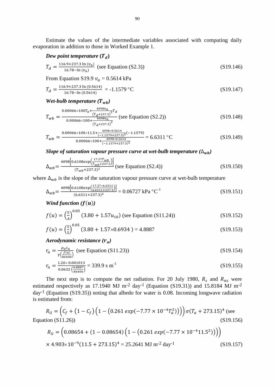
90

Estimate the values of the intermediate variables associated with computing daily evaporation in addition to those in Worked Example 1.

Dew point temperature (𝑻𝒅)

𝑇𝑑 = 116.9+237.3 ln (𝑣𝑎)16.78−ln (𝑣𝑎)


From Equation S19.9 𝑣𝑎 = 0.5614 kPa

𝑇𝑑 = 116.9+237.3 ln (0.5614)16.78−ln (0.5614)

= -1.1579 °C (S19.147)

Wet-bulb temperature (𝑻𝒘𝒃)

𝑇𝑤𝑏 =0.00066×100𝑇𝑎+

4098𝑣𝑎�𝑇𝑑+237.3�

2𝑇𝑑

0.00066×100+ 4098𝑣𝑎�𝑇𝑑+237.3�

2 (see Equation (S2.2)) (S19.148)

𝑇𝑤𝑏 =0.00066×100×11.5+ 4098×0.5614

(−1.1579+237.3)2(−1.1579)

0.00066×100+ 4098×0.5614(−1.1579+237.3)2

= 6.6311 °C (S19.149)

Slope of saturation vapour pressure curve at wet-bulb temperature (∆𝒘𝒃)

∆𝑤𝑏=4098�0.6108𝑒𝑥𝑝�

17.27𝑇𝑤𝑏𝑇𝑤𝑏+237.3��

(𝑇𝑤𝑏+237.3)2 (see Equation (S2.4)) (S19.150)

where ∆𝑤𝑏 is the slope of the saturation vapour pressure curve at wet-bulb temperature

∆𝑤𝑏=4098�0.6108𝑒𝑥𝑝�17.27×6.6311

6.6311+237.3��

(6.6311+237.3)2 = 0.06727 kPa °C-1 (S19.151)

Wind function (𝒇(𝒖))

𝑓(𝑢) = �5𝐴�0.05

(3.80 + 1.57𝑢10) (see Equation (S11.24)) (S19.152)

𝑓(𝑢) = �55�0.05

(3.80 + 1.57×0.6934 ) = 4.8887 (S19.153)

Aerodynamic resistance (𝒓𝒂)

𝑟𝑎 = 𝜌𝑎𝑐𝑎𝛾� 𝑓(𝑢)

86400� (see Equation (S11.23)) (S19.154)

𝑟𝑎 = 1.20× 0.001013

0.0632 �4.888786400�

= 339.9 s m-1 (S19.155)

The next step is to compute the net radiation. For 20 July 1980, 𝑅𝑠 and 𝑅𝑛𝑠 were estimated respectively as 17.1940 MJ m-2 day-1 (Equation (S19.31)) and 15.8184 MJ m-2 day-1 (Equation (S19.35)) noting that albedo for water is 0.08. Incoming longwave radiation is estimated from:

𝑅𝑖𝑙 = �𝐶𝑓 + �1 − 𝐶𝑓� �1 − �0.261 𝑒𝑥𝑝(−7.77 × 10−4𝑇𝑎2)��𝜎(𝑇𝑎 + 273.15)4 (see Equation (S11.26)) (S19.156)

𝑅𝑖𝑙 = �0.08654 + (1 − 0.08654) �1 − �0.261 𝑒𝑥𝑝(−7.77 × 10−411.52)��

× 4.903×10−9(11.5 + 273.15)4 = 25.2641 MJ m-2 day-1 (S19.157)

91

Outgoing longwave radiation as a function of wet-bulb temperature is estimated from:

𝑅𝑜𝑙𝑤𝑏 = 𝜎(𝑇𝑎 + 273.15)4 + 4𝜎(𝑇𝑎 + 273.15)3(𝑇𝑤𝑏 − 𝑇𝑎) (see Equation (S11.32))

(S19.158)

𝑅𝑜𝑙𝑤𝑏 = 4.903×10−9(11.5 + 273.15)4 + 4×4.903×10−9(11.5 + 273.15)3

(6.6311 − 11.5) = 29.9866 MJ m-2 day-1 (S19.157)

𝑄𝑤𝑏∗ = 𝑅𝑠(1 − 𝛼) + �𝑅𝑖𝑙 − 𝑅𝑜𝑙𝑤𝑏� (see Equation (S11.31)) (S19.160)

𝑄𝑤𝑏∗ = 15.8184 + 25.2641 −29.9866 = 11.0959 MJ m-2 day-1 (S19.161)

We now need to calculate the time constant (𝜏) and the equilibrium temperature (𝑇𝑒).

𝜏 = 𝜌𝑤𝑐𝑤ℎ𝑤4𝜎(𝑇𝑤𝑏+273.15)3+𝑓(𝑢)(Δwb+𝛾) (see Equation (S11.29)) (S19.162)

𝜏 = 997.9 ×0.00419×104×4.903×10−9(6.6311+273.15)3+4.8887(0.06727+0.0632 )

= 39.1739 days (S19.163)

𝑇𝑒 = 𝑇𝑤𝑏 + 𝑄𝑤𝑏∗

4𝜎(𝑇𝑤𝑏+273.15)3+𝑓(𝑢)(Δwb+𝛾) (see Equation (S11.30)) (S19.164)

𝑇𝑒 = 6.6311 + 11.09594×4.903×10−9(6.6311+273.15)3+4.8887(0.06727+0.0632 )

= 17.0269 °C (S19.165)

The next step is to estimate today’s water temperature given yesterday’s water temperature (assume 𝑇𝑤0 = 10.8734)

𝑇𝑤 = 𝑇𝑒 + (𝑇𝑤0 − 𝑇𝑒)exp �− 1𝜏� (see Equation (S11.28)) (S19.166)

𝑇𝑤 = 17.0269 + (10.8734 − 17.0269)exp �− 139.1739

� = 11.0285 °C (S19.167)

As we have an estimate of the water temperature, we can now estimate the change in heat storage (Gw), the slope of the saturation vapour pressure curve at water temperature (∆𝑤), the saturation vapour pressure at water temperature (𝑣𝑤∗ ), and the lake evaporation (𝐸𝑀𝑐𝐽).

Gw = 𝜌𝑤𝑐𝑤ℎ𝑤(𝑇𝑤 − 𝑇𝑤0) (see Equation (S11.33)) (S19.168)

Gw = 997.9 × 0.00419 × 10(11.0285 − 10.8734) = 6.4850 MJ m-2 day-1 (S19.169)

∆𝑤=4098�0.6108𝑒𝑥𝑝� 17.27𝑇𝑤

𝑇𝑤+237.3��

(𝑇𝑤+237.3)2 (see Equation (S2.4)) (S19.170)

∆𝑤=4098�0.6108𝑒𝑥𝑝�17.27×11.0285

11.0285 +237.3��

(11.0285 +237.3)2 = 0.08740 kPa °C-1 (S19.171)

𝑣𝑤∗ = 0.6108𝑒𝑥𝑝 � 17.27𝑇𝑤𝑇𝑤+237.3

� (see Equation (S2.5)) (S19.170)

𝑣𝑤∗ = 0.6108𝑒𝑥𝑝 �17.27×11.0285 11.0285 +237.3

� = 1.3152 kPa (S19.173)

The penultimate step is to recompute the net radiation given the water temperature.

𝑅𝑛𝑠 and 𝑅𝑖𝑙 will not change as they are essentially unaffected by the surface temperature. However, the outgoing longwave radiation (𝑅𝑜𝑙) is a function of water temperature which is now known.

𝑅𝑜𝑙 = 0.97 𝜎(𝑇𝑤 + 273.15)4 (see Equation (S11.27)) (S19.174)

92

𝑅𝑜𝑙 = 0.97×4.903×10−9(11.0285 + 273.15)4 = 31.0169 MJ m-2 day-1 (S19.175) Thus,

Q∗ = 𝑅𝑠(1 − 𝛼) + (𝑅𝑖𝑙 − 𝑅𝑜𝑙) (see Equation (S11.25)) (S19.176)

Q∗ = 15.8184 + (25.2641 − 31.0169) = 10.0656 MJ m-2 day-1

𝐸𝑀𝑐𝐽 = 1𝜆�Δw(Q∗−Gw)+86400𝜌𝑎𝑐𝑎�𝑣𝑤

∗ −𝑣𝑎�𝑟𝑎

Δw+𝛾� (see Equation (S11.22)) (S19.177)

𝐸𝑀𝑐𝐽 = 12.45

�0.087340(10.0656−6.4850)+86400×1.2×0.001013(1.3152−0.5614)

339.90.08732 +0.0632

� (S19.178)

𝐸𝑀𝑐𝐽 = 1.4796 mm day-1 (S19.179)

93

Supplementary Material Section S20 Listing of Fortran 90 version of Morton’s WREVAP

program The following program listing called Program WREVAP, which is a slightly modified

version of Morton’s WREVAP model, is written in Fortran 90 and follows closely the steps set out in Appendix C of Morton (1983a). The deep lake sub-routine is based on Morton (1986, Section 3).

The program uses a monthly time-step and requires the following input data: for each month, average daily temperature (°C), average daily relative humidity (%), and average daily sunshine hours. Other data required as input are mean annual precipitation (mm), latitude (decimal degree and negative for the southern hemisphere), and elevation of the station (m). For deep lake evaporation, lake salinity (ppm) and average lake depth (m) are also required. The outputs from the CRAE sub-model are monthly net solar radiation (mm), monthly potential evapotranspiration (mm), monthly wet areal evapotranspiration (mm) and monthly actual areal evapotranspiration (mm); from the CRWE sub-model are net radiation at the water surface, potential evaporation and actual shallow lake evaporation; and from CWLE sub-model are net radiation at the water surface, potential evaporation and actual deep lake evaporation.

Structure of Program WREVAP Program WREVAP calculates the actual evapotranspiration from a landscape

(catchment) environment, evaporation from a shallow lake and evaporation from a deep lake based on Morton’s (1983a,b; 1986) WREVAP program. The program WREVAP is a slightly modified version of Morton’s WREVAP and consists of one module (WREVAP data) and five subroutines (crae, crwe, crle1, crle2 and sub1). crae, crwe and crle represent Morton’s three program CRAE, CRWE and CRLE. Two versions of CRLE are include: crle1 calculates lake evaporation assuming the water depth in the lake is constant, and crle2 calculates lake evaporation assuming the water depth in the lake varies on a monthly basis.

The structure of Program WREVAP is shown in the figure below where: WREVAP data Variable declarations and constants crae Calculates the actual evapotranspiration from landscape crwe Calculates evaporation from shallow lake crle1 Calculates evaporation from deep lake (constant depth) crle2 Calculates evaporation from deep lake (variable depth) sub1 Calculates the solar radiation

WREVAP

WREVAPdata crae crwe crle 1 crle 2

sub 1 sub 1 sub 1 sub 1

94

Input data: latitude (degrees), station height (m), mean annual precipitation (mm year-1), number of months, monthly temperature (°C), relative humidity (%), sunshine hours (h), lake depth (m), salinity (ppm). The input data is supplied to the program via two files: a parameter file and a data file. Parameter file: WREVAP.par Example: Melbourne.dat File containing the climate and other data Melbourne.out Output file 1 Flag 1 – evapotranspiration from landscape 2 – evaporation from shallow lake 3 – evaporation from deep lake (constant depth) 4 – evaporation from deep lake (variable depth) Data file: Record

1 Station header 2 Latitude, station height, mean annual rainfall and number of months 3 Data header 4 year, month, number of days, temperature, relative humidity and sunshine

hours . “ “ “ . “ “ “ Example: Melbourne.dat (for crae and crwe) 86282 86 MELBOURNE AIRPORT -37.666 113.4 660 201 Year Month Day Temperature RH SH 1993 5 31 12.54 72.58 8.88 1993 6 30 10.12 76.73 7.08 1993 7 31 9.90 75.74 10.03 1993 8 31 11.62 69.44 -9999 1993 9 30 12.12 75.97 9.63 1993 10 31 13.16 70.58 11.20 1993 11 30 15.15 71.00 10.95 1993 12 31 16.80 68.94 9.53 . . Example: ThomsonReservoir.dat (for crle1) Thomson Reservoir -37.752 415.0 1090 36 22.95 23 Year Month Day Temperature RH SH 2007 3 31 16.59 69.96 8.02 2007 4 30 13.45 74.71 7.31 2007 5 31 12.56 73.88 5.20 2007 6 30 6.94 85.04 3.91 2007 7 31 6.98 79.93 4.45 2007 8 31 9.33 72.12 6.58 2007 9 30 9.77 69.64 7.03

95

2007 10 31 12.77 64.85 7.86 2007 11 30 15.43 75.45 8.42 2007 12 31 17.28 69.95 8.43 . . Example: ThomsonReservoirVD.dat (for crle2) Thomson Reservoir -37.752 415.0 1090 36 23 Year Month Day Temperature RH SH Depth 2007 3 31 16.59 69.96 8.02 22.52 2007 4 30 13.45 74.71 7.31 21.99 2007 5 31 12.56 73.88 5.20 21.69 2007 6 30 6.94 85.04 3.91 21.79 2007 7 31 6.98 79.93 4.45 23.39 2007 8 31 9.33 72.12 6.58 24.26 2007 9 30 9.77 69.64 7.03 24.86 2007 10 31 12.77 64.85 7.86 25.26 2007 11 30 15.43 75.45 8.42 25.52 2007 12 31 17.28 69.95 8.43 25.62 . .

96

Program WREVAP (Fortran 90) Lines designated as !C-1 to !C-39 identify the equivalent equations in Morton (1983a,

Appendix C) and those designated as ! (3) to ! (8) are from Morton (1986). A list of variables is provided at the end of the program.

A web-site for the Fortran listing of Morton’s WREVAP program is available at

http://people.eng.unimelb.edu.au/mpeel/morton.html. On this site corrections to the code will be listed, updated versions of WREVAP code provided and .exe files will be available.

Module WREVAPdata implicit none save character(len=80) :: fn integer :: year, month, nd, ios, j, im, nm, nn(12) real :: phid, h, p, pa, pps, azd, td, t, s, v, vd, delta, &

theta, tc, c0, c1, c2, w, phi, rh real :: alpha(2) = (/17.27, 21.88/), beta(2) = (/237.3, 265.5/),&

pi = 3.14159254, gamma(2), ftz(2), fz(2), az, azz, cz, & cosz, comega, eta, ge, z, tmp, a0, g0, b, rt, rtc, & zeta, ft, lambda, et, etp, tau, rho, delp, delt, vp, &

tp, es, d, salt, omega, taua, g, a, b0, rtp, etw, b1, & b2, ltheat, xm(4,12), gdew, rw, ep, ew

end Module WREVAPdata program WREVAP ! Calculates Morton's ET ! 05 April 2012 use WREVAPdata implicit none integer :: flag open (10, file = 'WREVAP.par', status = 'old') read (10, 100) fn; 100 format(a) open (11, file = fn, status = 'old')

! Input data file read (10, 100) fn open (21, file = fn) ! Output file read (11, 100) fn write (21, 100) fn read (10, *) flag if (flag == 1) then ! b0 = 1.; b1 = 14.; b2 = 1.20; fz(1) = 28. !Morton's values b0 = 1.; b1 = 13.4; b2 = 1.13; fz(1) = 29.2 ! QJ's values es = 5.22e-8 write (21, '("fz, b1, and b2", 3f8.2)'), fz(1), b1, b2 read (11, *) phid, h, pa, nm write (21, 200) phid, h, pa, nm 200 format('Latitude =', f7.2, ' Station height =', f8.2, & ' m Mean annual precipitation =', f8.1, ' mm'/ & '# of months =', i5 ) write (21, 201) 201 format(' Year Month Temp Rel Hum Sunshine’ &

‘Net Rad PET WET AET ft'/ &

http://people.eng.unimelb.edu.au/mpeel/morton.html

97

' (oC) (%) (Ratio) (mm)’ & ‘ (mm) (mm) (mm)')

else b0 = 1.12 b1 = 13. b2 = 1.12 es = 5.5e-8 fz(1) = 25. if (flag == 2) then read (11, *) phid, h, pa, nm write (21, 200) phid, h, pa, nm else if (flag == 3 ) then read (11, *) phid, h, pa, nm, d, salt write (21, 202) phid, h, pa, d, salt, nm 202 format('Latitude =', f7.2, ' Station height =', &

f8.2, ' m', ' Mean annual precipitation =', & f8.1, ' mm'/ ' Lake depth =', f7.2, ' m', &

' Salt =', f8.1, ' ppm', ' # of months =', i5 ) else if (flag == 4 ) then read (11, *) phid, h, pa, nm, salt write (21, 203) phid, h, pa, salt, nm 203 format('Latitude =', f7.2, ' Station height =', &

f8.2, ' m', ' Mean annual precipitation =', & f8.1, ' mm'/ ' Salt =', f8.1, ' ppm', &

' # of months =', i5 ) end if end if read (11, *) ! Skip a line phi = phid*pi/180. ! Compute the ratio of atmospheric pressure at the station to that ! at sea level pps = ((288. - 0.0065*h)/288)**5.256 !C-1 p = pps*1013. ! Estimate the zenith value of the dry season snow free clear sky ! albedo azd = 0.26 - 0.00012*pa*(1 + abs(phid/42) + &

(phid/42)**2)*pps**0.5 !C-2 if (azd < 0.11) azd = 0.11 if (azd > 0.17) azd = 0.17 gamma(1) = 0.66*pps gamma(2) = gamma(1)/1.15 fz(2) = fz(1)*1.15 ftz(1) = fz(1)*sqrt(1./pps) ftz(2) = ftz(1)*1.15 nn = 0 ; xm =0. if (flag == 1) then call crae(1) else if (flag == 2) then write (21, 204) 204 format(' Year Month Temp Rel Hum Sunshine ‘, &

‘Net Rad PET AET'/ & ‘ (oC) (%) (Ratio) (mm)’, &

’ (mm) (mm)’) call crwe(2)

98

else if (flag == 3) then write (21, 204) call crle1(3) else if (flag == 4) then write (21, 205) 205 format(‘ Year Month Temp Rel Hum Sunshine’, &

’ Depth Net Rad PET AET’/ & ‘ (oC) (%) (Ratio)’, &

‘ (m) (mm) (mm) (mm)') call crle2(4) end if end program WREVAP subroutine crae(flag) ! Calculates the actual evapotranspiration from landscape use WREVAPdata implicit none integer :: flag do im = 1, nm read (11, *, iostat = ios) year, month, nd, t, rh, s if (ios < 0) exit if (s < 0. .OR. rh < 0. .OR. t < -999.) cycle call sub1(flag) ! Estimate the net radiation for soil-plant surfaces at air ! temperature (rt), the stability factor (sf), the vapour ! pressure coefficient (ft) and the heat transfer ! coefficient (lambda) rt = (1. - a)*g - b !C-27 rtc = rt !C-28 if (rtc < 0.) rtc = 0. !C-28a zeta = 1./(0.28*(1. + vd/v) + delta*rtc*pps**0.5/ &

(gamma(j)*b0*fz(j)*(v - vd))) !C-29 if (zeta < 1.) zeta = 1. !C-29a ft = fz(j)/zeta/pps**0.5 !C-30 lambda = gamma(j) + 4.*es*(t + 273)**3/ft !C-31 ! Estimate the final values from the following quickly ! converging iterative solution of the vapour transfer ! and energy balance equations tp = t

vp = v delp = delta do delt = (rt/ft + vd - vp +lambda*(t - tp))/ &

(delp + lambda) !C-32 tp = tp + delt !C-33 vp = 6.11*exp(alpha(j)*tp/(tp + beta(j))) !C-34 delp = alpha(j)*beta(j)*vp/(tp + beta(j))**2 !C-35 if (abs(delt) < 0.01) exit end do ! Estimate the potential evapotranspiration (etp), the net ! radiation for soil-plant surfaces at equilibrium temperature ! (rtp) and the wet-environment areal evapotranspiration (etw) etp = rt - lambda*ft*(tp - t) !C-36 rtp = etp + gamma(j)*ft*(tp - t) !C-37

99

etw = b1 + b2*rtp/(1. + gamma(j)/delp) !C-38 if (etw < etp/2.) etw = etp/2. !C-38a if (etw > etp) etw = etp !C-38a ! Estimate the areal evapotranspiration (et) from the ! complementary relationship et = 2.*etw - etp !C-39 ltheat = 28.5 if (t < 0.) ltheat = 28.5*1.15 et = nd*et/ltheat rt = nd*rt/ltheat etp = nd*etp/ltheat etw = nd*etw/ltheat write (21, 201) year, month, t, rh, s, rt, etp, etw, et, ft 201 format(i5, i3, 8f10.2) xm(1,month) = xm(1,month) + rt xm(2,month) = xm(2,month) + etp xm(3,month) = xm(3,month) + etw xm(4,month) = xm(4,month) + et nn(month) = nn(month) + 1 end do write (21, 202) 202 format(/10x,'Mean Values'/'Month Net Rad PET’ &

‘ WET AET # of months') do month = 1, 12 xm(:,month) = xm(:,month)/nn(month) write (21, 203) month, (xm(j,month), j = 1, 4), nn(month) 203 format(i5, 4f10.2, i5) end do write (21, 204) (sum(xm(j,:)), j = 1, 4) 204 format('Annual', f9.1, 3f10.2) end subroutine crae subroutine sub1(flag) use WREVAPdata implicit none integer :: flag if (t < 0.) then j = 2 else j = 1 end if ! Compute the saturation vapour pressure at td (vd), at t (v) and ! the slope of the saturation vapour pressure at t (delta) v = 6.11*exp(alpha(j)*t/(t + beta(j))) !C-4 ! Calculate dew point temperature from relative humidity ! (Lawrence 2005) gdew = 17.625*t/(243.04 + t) + log(rh/100.) td = 243.04*gdew/(17.625 - gdew) vd = 6.11*exp(17.27*td/(td + 237.3)) delta = alpha(j)*beta(j)*v/(t + beta(j))**2 !C-5 ! Compute various angles and functions leading up to an estimate ! of the extra-atmospheric global radiation (ge) theta = 23.2*sin((29.5*month - 94.)*pi/180.)*pi/180. !C-6 z = phi - theta cosz = cos(z) !C-7

100

if (cosz < 0.001) cosz = 0.001 !C-7a if (cosz > 1.) cosz = 1. z = acos(cosz) comega = 1. - cosz/cos(phi)/cos(theta) !C-8 if (comega < -1.) comega = -1. !C-8a omega = acos(comega) cz = cosz + (sin(omega)/omega - 1.)*cos(phi)*cos(theta) !C-9 eta = 1. + sin((29.5*month - 106)*pi/180.)/60. !C-10 ge = 1354*omega*cz/pi/eta/eta !C-11 ! Estimate the zenith value of snow-free clear-sky albedo (azz), ! zenith value of clear-sky albedo (az) and the clear sky ! albedo (a0) if (flag > 1) then

azz = 0.05 else azz = azd !C-12 if (azz > 0.5*(0.91 - vd/v)) azz = 0.5*(0.91 - vd/v) !C-12a end if c0 = v - vd !C-13 if (c0 < 0.) c0 = 0. !C-13a if (c0 > 1.) c0 = 1. !C-13a az = azz + (1. - c0*c0)*(0.34 - azz) !C-14 a0 = az*(exp(1.08) - (2.16*cosz/pi + & sin(z))*exp(0.012*z*180./pi))/1.473/(1. - sin(z)) !C-15 ! Estimate precipitable water (w) and a turbidity coefficient (tc) w = vd/(0.49 + t/129.) !C-16 c1 = 21 - t !C-17 if (c1 < 0.) c1 = 0. !C-17a if (c1 > 5.) c1 = 5. !C-17a tc = (0.5 + 2.5*cz*cz)*exp(c1*(pps - 1.)) !C-18 ! Compute the transmittancy of clear skies to direct beam ! solar radiation (tau) tau = exp(-0.089*(pps/cz)**0.75 - 0.083*(tc/cz)**0.90 - &

0.029*(w/cz)**0.60) !C-19 ! Estimate the part of tau that is the result of absorption (taua) taua = exp(-0.0415*(tc/cz)**0.90 - (0.0029**0.5)* &

(w/cz)**0.3) !C-20 tmp = exp(-0.0415*(tc/cz)**0.90 - 0.029*(w/cz)**0.6) if (taua < tmp) taua = tmp !C-20a ! Compute the clear-sky global radiation (g0) and the incident ! global radiation (g) g0 = ge*tau*(1. + (1. - tau/taua)*(1. + a0*tau)) !C-21 s = s*pi/24./omega if (s > 1.) s = 0.999 g = s*g0 + (0.08 + 0.30*s)*(1. - s)*ge !C-22 ! Estimate the average albedo (a) a = a0*(s + (1. - s)*(1. - z*180/pi/330)) !C-23 ! Estimate the proportional increase in atmospheric radiation ! due to clouds (rho) c2 = 10.*(vd/v - s - 0.42) !C-24 if (c2 < 0.) c2 = 0. !C-24a if (c2 > 1.) c2 = 1. !C-24a rho = 0.18*((1. - c2)*(1. - s)**2 + c2*(1. - s)**0.5)/pps !C-25 ! Calculate the net long-wave radiation loss for soil-plant ! surface at air temperature (b)

101

b = es*(t + 273)**4*(1. - (0.71 + 0.007*vd*pps)*(1. + rho))!C-26 tmp = 0.05*es*(t + 273)**4 if ( b < tmp) b = tmp !C-26a end subroutine sub1 subroutine crwe(flag) ! Calculates Morton's ET - Shallow lake evaporation ! 05 April 2012 use WREVAPdata implicit none integer :: flag do im = 1, nm read (11, *, iostat = ios) year, month, nd, t, rh, s if (ios < 0) exit if (s < 0. .OR. rh < 0. .OR. t < -999.) cycle call sub1(flag) ! Estimate the net radiation for water surface at air ! temperature (rw), ! the stability factor (sf), the vapour pressure ! coefficient (ft) and the heat transfer coefficient (lambda) rw = (1. - a)*g - b rtc = rw if (rtc < 0.) rtc = 0. zeta = 1./(0.28*(1. + vd/v) + delta*rtc*pps**0.5/ &

(gamma(j)*b0*fz(j)*(v - vd))) if (zeta < 1.) zeta = 1. ft = fz(j)/zeta/pps**0.5 lambda = gamma(j) + 4.*es*(t + 273)**3/ft ! Estimate the final values from the following quickly ! converging iterative solution of the vapour transfer ! and energy balance equations tp = t vp = v delp = delta do delt = (rw/ft + vd - vp +lambda*(t - tp))/(delp + lambda) tp = tp + delt

vp = 6.11*exp(alpha(j)*tp/(tp + beta(j))) delp = alpha(j)*beta(j)*vp/(tp + beta(j))**2 if (abs(delt) < 0.01) exit

end do ! Estimate the potential evaporation (ep), the net radiation ! for soil-plant surfaces at equilibrium temperature (rtp) ! and the shallow lake evaporation (ew) ep = rw - lambda*ft*(tp - t) rtp = ep + gamma(j)*ft*(tp - t) ew = b1 + b2*rtp/(1. + gamma(j)/delp) if (ew < ep/2.) ew = ep/2. if (ew > ep) ew = ep ltheat = 28.5 if (t < 0.) ltheat = 28.5*1.15 ep = nd*ep/ltheat rw = nd*rw/ltheat ew = nd*ew/ltheat

102

write (21, 201) year, month, t, rh, s, rw, ep, ew 201 format(i5, i3, 6f10.2) xm(1,month) = xm(1,month) + rw xm(2,month) = xm(2,month) + ep xm(3,month) = xm(3,month) + ew nn(month) = nn(month) + 1 end do write (21, *) ' Mean values' write (21, *) 'Month Net Rad PET AET' do month = 1, 12 xm(:,month) = xm(:,month)/nn(month) write (21, 203) month, (xm(j,month), j = 1, 3) 203 format(i5, 4f10.2) end do write (21, 204) (sum(xm(j,:)), j = 1, 3) 204 format('Annual', f9.1, 3f10.2) end subroutine crwe subroutine crle1(flag) ! Calculates Morton's ET - Deep lake evaporation ! 05 April 2012 use WREVAPdata implicit none integer, parameter :: nmx = 360 integer :: ic, iy(nmx), mon(nmx), tnd(nmx), flag real :: tgw(nmx), tv(nmx), tvd(nmx), ts(nmx), gl(nmx), &

tt(nmx), trh(nmx), tdelta(nmx) do im = 1, nm

read (11, *, iostat = ios) year, month, nd, t, rh, s if (ios < 0) exit if (s < 0. .OR. rh < 0. .OR. t < -999.) cycle call sub1(flag) tgw(im+12) = (1. - a)*g - b tt(im) = t trh(im) = rh ts(im) = s tv(im) = v tvd(im) = vd tdelta(im) = delta iy(im) = year tnd(im) = nd mon(im) = month end do call deepLake(nmx, nm, tgw, gl, d, salt) do im = 1, nm t = tt(im) rh = trh(im) s = ts(im) v = tv(im) vd = tvd(im) delta = tdelta(im) ! Estimate the net radiation for water surface at air ! temperature (rw), ! the stability factor (sf), the vapour pressure coefficient ! (ft) and the heat transfer coefficient (lambda)

103

rw = gl(im) rtc = rw if (rtc < 0.) rtc = 0. zeta = 1./(0.28*(1. + vd/v) + delta*rtc*pps**0.5/ &

(gamma(j)*b0*fz(j)*(v - vd))) !C-29 if (zeta < 1.) zeta = 1. !C-29a ft = fz(j)/zeta/pps**0.5 !C-30 lambda = gamma(j) + 4.*es*(t + 273)**3/ft !C-31 ! Estimate the final values from the following quickly ! converging iterative solution of the vapour transfer ! and energy balance equations tp = t vp = v delp = delta ic = 0 do delt = (rw/ft + vd - vp +lambda*(t - tp))/ &

(delp + lambda) !C-32 tp = tp + delt !C-33 vp = 6.11*exp(alpha(j)*tp/(tp + beta(j))) !C-34 delp = alpha(j)*beta(j)*vp/(tp + beta(j))**2 !C-35 if (abs(delt) < 0.01) exit ic = ic + 1 if (ic > 100) then print *, 'Did not converge for month', im exit end if end do ! Estimate the potential evaporation (ep), the net radiation ! for soil-plant surfaces at equilibrium temperature (rtp) and ! the deep lake evaporation (ew) ep = rw - lambda*ft*(tp - t) rtp = ep + gamma(j)*ft*(tp - t) ew = b1 + b2*rtp/(1. + gamma(j)/delp) if (ew < ep/2.) ew = ep/2. if (ew > ep) ew = ep ltheat = 28.5 if (t < 0.) ltheat = 28.5*1.15 nd = tnd(im) ep = nd*ep/ltheat rw = nd*rw/ltheat ew = nd*ew/ltheat write (21, 201) iy(im), mon(im), t, rh, s, rw, ep, ew 201 format(i5, i3, 6f10.2) xm(1,mon(im)) = xm(1,mon(im)) + rw xm(2,mon(im)) = xm(2,mon(im)) + ep xm(3,mon(im)) = xm(3,mon(im)) + ew nn(mon(im)) = nn(mon(im)) + 1 end do write (21, *) ' Mean values' write (21, *) 'Month Net Rad PET AET' do month = 1, 12 xm(:,month) = xm(:,month)/nn(month) write (21, 203) month, (xm(j,month), j = 1, 3) 203 format(i5, 4f10.2)

104

end do write (21, 204) (sum(xm(j,:)), j = 1, 3) 204 format('Annual', f9.1, 3f10.2) end subroutine crle1 subroutine deepLake(nmx, nm, tgw, gl, d, salt) ! Calculates the available solar and waterborne heat(gl) using ! Morton 1986 implicit none integer :: im, nmx, nm, ti, t1, i, i1, ii real :: gw(nmx), tgw(nmx), gl(nmx), t0, t, glb, gle, & salt, d, f, k t0 = 0.96 + 0.013*d !(6) if (t0 < 0.039*d) t0 = 0.039*d if (t0 > 0.13*d) t0 = 0.13*d t = t0/(1. + salt/27000)**2 !(7) if (t > 6.) t = 6. k = t0/(1. + (d/93)**7) !(8) ! Calculates the delayed solar and waterborne energy (gw) ti = int(t) t1 = ti + 1 f = t - ti i = 12 tgw(1:12) = tgw(13:24) do im = 1, nm i = i + 1 i1 = i - t1 ii = i - ti gw(im) = tgw(ii) + f*(tgw(i1) - tgw(ii)) !(3) end do ! Calculates the available solar and waterborne heat(gl) glb = 50. do i = 1, 2 do im = 1, 12 gle = glb + (gw(im) - glb)/(k + 0.5) !(4) gl(im) = (glb + gle)/2. !(5) glb = gle end do end do do im = 1, nm gle = glb + (gw(im) - glb)/(k + 0.5) !(4) gl(im) = (glb + gle)/2. !(5) glb = gle end do end subroutine deepLake subroutine crle2(flag) ! Calculates Morton's ET - Deep lake evaporation ! 05 April 2012 use WREVAPdata implicit none integer, parameter :: nmx = 360 integer :: ic, iy(nmx), mon(nmx), tnd(nmx), flag real :: tgw(nmx), tv(nmx), tvd(nmx), ts(nmx), gl(nmx), &

tt(nmx), trh(nmx), tdelta(nmx), da(nmx)

105

do im = 1, nm read (11, *, iostat = ios) year, month, nd, t, rh, s, da(im) if (ios < 0) exit if (s < 0. .OR. td < 0. .OR. t < -999.) cycle call sub1(flag) tgw(im+12) = (1. - a)*g - b tt(im) = t trh(im) = rh ts(im) = s tv(im) = v tvd(im) = vd tdelta(im) = delta iy(im) = year mon(im) = month tnd(im) = nd end do call deepLakeVD(nmx, nm, tgw, gl, da, salt) do im = 1, nm t = tt(im) rh = trh(im) s = ts(im) v = tv(im) vd = tvd(im) delta = tdelta(im) ! Estimate the net radiation for water surface at air ! temperature (rw), ! the stability factor (sf), the vapour pressure coefficient ! (ft) and the heat transfer coefficient (lambda) rw = gl(im) rtc = rw if (rtc < 0.) rtc = 0. zeta = 1./(0.28*(1. + vd/v) + delta*rtc*pps**0.5/ &

(gamma(j)*b0*fz(j)*(v - vd))) !C-29 if (zeta < 1.) zeta = 1. !C-29a ft = fz(j)/zeta/pps**0.5 !C-30 lambda = gamma(j) + 4.*es*(t + 273)**3/ft !C-31 ! Estimate the final values from the following quickly ! converging iterative solution of the vapour transfer and ! energy balance equations tp = t vp = v delp = delta ic = 0 do delt = (rw/ft + vd - vp +lambda*(t - tp))/(delp + lambda)

!C-32 tp = tp + delt !C-33 vp = 6.11*exp(alpha(j)*tp/(tp + beta(j))) !C-34 delp = alpha(j)*beta(j)*vp/(tp + beta(j))**2 !C-35 if (abs(delt) < 0.01) exit ic = ic + 1 if (ic > 100) then print *, 'Did not converge for month', im exit end if

106

end do ! Estimate the potential evaporation (ep), the net radiation ! for soil-plant ! surfaces at equilibrium temperature (rtp) and the deep lake ! evaporation (ew) ! ep = rw - lambda*ft*(tp - t) rtp = ep + gamma(j)*ft*(tp - t) ew = b1 + b2*rtp/(1. + gamma(j)/delp) if (ew < ep/2.) ew = ep/2. if (ew > ep) ew = ep ltheat = 28.5 if (t < 0.) ltheat = 28.5*1.15 nd = tnd(im) ep = nd*ep/ltheat rw = nd*rw/ltheat ew = nd*ew/ltheat write (21, 201) iy(im), mon(im), t, rh, s, da(im), rw, ep, ew 201 format(i5, i3, 7f10.2) xm(1,mon(im)) = xm(1,mon(im)) + rw xm(2,mon(im)) = xm(2,mon(im)) + ep xm(3,mon(im)) = xm(3,mon(im)) + ew nn(mon(im)) = nn(mon(im)) + 1 end do write (21, *) ' Mean values' write (21, *) 'Month Net Rad PET AET' do month = 1, 12 xm(:,month) = xm(:,month)/nn(month) write (21, 203) month, (xm(j,month), j = 1, 3) 203 format(i5, 4f10.2) end do write (21, 204) (sum(xm(j,:)), j = 1, 3) 204 format('Annual', f9.1, 3f10.2) end subroutine crle2 subroutine deepLakeVD(nmx, nm, tgw, gl, da, salt) ! Calculates the available solar and waterborne heat(gl) using ! Morton 1986 implicit none integer :: im, nmx, nm, ti, t1, i, i1, ii real :: gw(nmx), tgw(nmx), gl(nmx), t0, t, glb, gle, salt, &

d, f, da(nmx), k tgw(1:12) = tgw(13:24) i = 12 do im = 1, nm d = da(im) t0 = 0.96 + 0.013*d !(6) if (t0 < 0.039*d) t0 = 0.039*d if (t0 > 0.13*d) t0 = 0.13*d t = t0/(1. + salt/27000)**2 !(7) if (t > 6.) t = 6. k = t0/(1. + (d/93)**7) !(8) ! Calculates the delayed solar and waterborne energy (gw) ti = int(t)

107

t1 = ti + 1 f = t - ti i = i + 1 i1 = i - t1 ii = i - ti gw(im) = tgw(ii) + f*(tgw(i1) - tgw(ii)) !(3) end do ! Calculates the available solar and waterborne heat(gl) glb = 50. do i = 1, 2 do im = 1, 12 gle = glb + (gw(im) - glb)/(k + 0.5) !(4) gl(im) = (glb + gle)/2. !(5) glb = gle end do end do do im = 1, nm gle = glb + (gw(im) - glb)/(k + 0.5) !(4) gl(im) = (glb + gle)/2. !(5) glb = gle end do end subroutine deepLakeVD

108

Key variables used in Program WREVAP

Variable Description a average albedo a0 clear-sky albedo alpha constant used in estimating vapour pressure - changes at 0o C az zenith value of clear-sky albedo azd zenith value of the dry season snow free clear sky albedo azz zenith value of snow-free clear-sky albedo b net longwave radiation loss for soil-plant surface at air temperature beta constant used in estimating vapour pressure - changes at 0o C cosz cosine of the noon angular zenith distance of the sun cz cosine of the average angular zenith distance of the sun delt correction to tp in iteration process delta slope of the saturation vapour pressure at t es surface emissivity times the Stefan-Boltzmann constant et areal evapotranspiration eta radius vector of the sun etp potential evapotranspiration etw wet-environment areal evapotranspiration ft vapour pressure coefficient g incident global radiation g0 clear-sky global radiation gamma psychrometric constant - changes at 0o C ge extra-atmospheric global radiation in Wm-2 gl available solar and waterborne heat glb value of gl at the beginning gle value of gl at the end gw delayed solar and waterborne heat h station height iy array to store year k storage constant lambda heat transfer coefficient ltheat latent heat of vaporisation water mon array to store month nd number of days in a month nm number of months omega angle in radians the earth rotates between sunrise and noon p atmospheric pressure pa mean annual rainfall phi latitude in radians phid latitude in degrees pps ratio of atmospheric pressure at the station to that at sea level rho proportional increase in atmospheric radiation due to clouds rt net radiation for soil-plant surfaces at air temperature rtp net radiation for soil-plant surfaces at equilibrium temperature rw net radiation for water surface at air temperature s ratio of observed to maximum possible sunshine duration sf the stability factor

109

t average air temperature t lake delay time in months tau transmittancy of clear skies to direct beam soar radiation taua part of tau that is the result of absorption tc turbidity coefficient td average dew point temperature tdelta array to store delta theta declination of sun tnd array to store nd to soft water delay time in months tp potential evapotranspiration equilibrium temperature trh array to store rh ts array to store s tt array to store t tv array to store v tvd array to store vd v saturation vapour pressure at t vd saturation vapour pressure at td vp saturation vapour pressure at tp w precipitable water xm variable to calculate mean monthly values

110

Supplementary Material Section S21 Worked example of Morton’s CRAE, CRWE and CRLE

models within the WREVAP framework List of variables that are used in this section are taken from Morton (1983a, Appendix D) and

from Morton (1986))

(Note these variables are different to those adopted in Section S20 and in the main text and other sections.)

Variable Description Units

𝑎 Average albedo dimensionless

𝑎0 Clear-sky albedo dimensionless

𝑎𝑧 Zenith value of clear-sky albedo dimensionless

𝑎𝑧𝑑 Zenith value of the dry-season snow-free clear sky albedo dimensionless

𝑎𝑧𝑧 Zenith value of clear-sky snow-free albedo dimensionless

𝐵 Net longwave radiation loss for soil-plant surface at air temperature W m-2

𝑏0 Constant undefined

𝑏1 Constant W m-2

𝑏2 Constant undefined

𝑐0 𝜐 − 𝜐𝐷 mbar

𝑐1 Working variable °C

𝑐2 Working variable dimensionless

𝐸𝑃 Potential evaporation W m-2, mm month-1

𝐸𝑇 Actual areal evapotranspiration W m-2, mm month-1

𝐸𝑇𝑃 Potential evapotranspiration W m-2, mm month-1

𝐸𝑇𝑊 Wet-environment areal evapotranspiration W m-2, mm month-1

𝐸𝑊 Shallow lake evaporation W m-2, mm month-1

𝑓𝑇 Vapour transfer coefficient W m-2 mbar-1

𝑓𝑧 Constant used in estimating 𝑓𝑇 W m-2 mbar-1

𝐺 Incident global radiation W m-2

𝐺𝐸 Extra-atmospheric global radiation W m-2

𝐺𝐿 Available (routed) solar and waterborne energy W m-2

𝐺𝐿𝐵 Available solar and waterborne heat energy at the beginning W m-2

111

of the month

𝐺𝐿𝐸 Available solar and waterborne heat energy at the end of the month W m-2

𝐺𝑜 Clear-sky global radiation W m-2

𝐺𝑊0 Solar plus waterborne heat input W m-2

𝐺𝑊𝑡 Delayed solar and waterborne energy inputs W m-2

𝐺𝑊[𝑡],

𝐺𝑊[𝑡+1]

Value of 𝐺𝑊0 computed [𝑡𝐿] and [𝑡𝐿 + 1] months W m-2

ℎ� Average depth of lake m

𝐻 Site elevation m

𝑖 Month number dimensionless

𝑗 Turbidity coefficient undefined

𝑃𝐴 Mean annual rainfall mm year-1

𝑝 Atmospheric pressure at station mbar

𝑝𝑠 Atmospheric pressure at mean sea level mbar 𝑝𝑝𝑠

Ratio of atmospheric pressure at station to atmospheric pressure at mean sea level dimensionless

𝑅𝐻 Mean daily relative humidity %

𝑅𝑛𝑙 Net longwave radiation W m-2

𝑅𝑠 Measured incoming solar radiation W m-2

𝑅𝑇 Net radiation at soil-plant surface at air temperature W m-2 𝑅𝑇𝐶 𝑅𝑇 with 𝑅𝑇𝐶 ≥ 0 W m-2 𝑅𝑇𝑃 Net radiation at the soil-plant surface for equilibrium

temperature W m-2

𝑅𝑊 Net radiation for water surface at air temperature W m-2

𝑠 Average lake salinity ppm

𝑆 Ratio of observed to maximum possible sunshine duration dimensionless

𝑆𝑐 Storage coefficient months

𝑡0 Soft water delay time months

𝑡𝐿 Lake lag or delay time months

[𝑡𝐿] Integral component of the lake lag months

𝑇 Mean daily air temperature for month °C 𝑇𝐷 Mean daily dew point temperature for month °C 𝑇𝑃 Equilibrium temperature °C

𝑇𝑃′ Trial value of 𝑇𝑃 in iteration process °C

112

𝑊 Precipitable water vapour mm

𝑍 Noon angular zenith distance of sun radian

𝑧 Average angular zenith distance of the Sun radian

𝛼 Constant Equations (S21.12 and S21.78); albedo Equation (S21.97)

°C; dimensionless

𝛽 Constant Equations (S21.12 and S21.78) °C

γ Psychrometric constant mbar °C-1

δℎ Water borne heat input W m-2

∆ Saturation vapour pressure curve at 𝑇 mbar °C-1

∆𝑃 Slope of saturation vapour pressure curve at 𝑇𝑃 mbar °C-1

∆𝑇′ Slope of saturation vapour pressure curve at 𝑇𝑃′ mbar °C-1

[𝛿𝑇𝑃] Adjustment to 𝑇𝑃 in iteration process °C

𝜀 Surface emissivity dimensionless

𝜉 Stability factor undefined

𝜂 Radius vector of sun undefined

𝜃 Declination of sun radians

𝜆 Heat transfer coefficient mbar °C-1

𝜌 Proportional increase in atmospheric radiation due to clouds dimensionless

𝜎 Stefan-Boltzmann constant W m-2 K-4

𝜏 Transmittancy of clear sky to direct beam radiation undefined

𝜏𝑎 Proportion of 𝜏 that is the result of absorption undefined

𝜐 Mean daily saturation vapour pressure at air temperature for month mbar

𝜐𝐷 Mean daily saturation vapour pressure at dew point temperature for month mbar

𝜐𝑃 Mean daily saturation vapour pressure at equilibrium temperature for month mbar

𝜐𝑃 ′ Trial value of 𝜐𝑃 in iteration process mbar

Ø Latitude degree, radians

𝜔 Angle the earth rotates between sunrise and noon radian

CRAE: Estimate actual evaporation Use Morton’s CRAE model to estimate the potential and actual evaporation for July

1980 at Alice Springs (Bureau of Meteorology, Australia station number 15590). Although the general methodology is presented in Section S7, the following procedure follows the detailed steps in Morton (1983a, Appendix C) and the Fortran program in Section S20. The symbols adopted here are those used by Morton and are different to those used in the Morton Fortran program (Section S20) and in the other sections.

113

The site conditions at Alice Spring automatic weather station are as follows:

Latitude (Ø) -23.7951 °S (negative for southern hemisphere) -0.4153 radian

Site elevation (𝐻) 546 m Mean annual rainfall (𝑃𝐴) 285.8 mm year-1

The meteorological data for July 1980 is: Mean daily air temperature (𝑇 ) 11.8 °C day-1 Mean daily relative humidity (𝑅𝐻 ) 55.5 % day-1 Mean daily sunshine hours 8.35 hour day-1

Because Morton assumes dew point temperature is available to estimate saturation vapour pressure rather than relative humidity, we carry out the following preliminary calculations to estimate dew point temperature (𝑇𝐷) as follows (Lawrence, 2005, Equation 8):

𝑇𝐷 =243.04�𝑙𝑛�𝑅𝐻100�+

17.625 𝑇243.04+𝑇�

17.625−𝑙𝑛�𝑅𝐻100�−17.625 𝑇243.04+𝑇

(S21.1)

where 𝑇 is air temperature (°C), 𝑅𝐻 is the relative humidity (%). For July 1980, Alice Springs

𝑇𝐷 =243.04�𝑙𝑛�55.5

100�+17.625×11.8243.04+11.8�

17.625−𝑙𝑛�55.5100�−

17.625×11.8243.04+11.8

= 3.1755 °C (S21.2)

To maintain consistency with Morton’s (1983a) procedure, we adopt the units he used in his Appendix C namely W m-2 for radiation, mbar for vapour pressure and °C for temperature. We also adopt Morton’s nomenclature and record below Morton’s equation numbers in italics.

The following two equations refer to the site conditions.

Equation C-1: Compute the ratio ( 𝑝𝑝𝑠

) of atmospheric pressure at Alice Springs station (𝑝) to that at sea level (𝑝𝑠):

𝑝𝑝𝑠

= [(288 − 0.0065𝐻)/288)]5.256 (S21.3)

𝑝𝑝𝑠

= [(288 − 0.0065 × 546)/288)]5.256 = 0.9369 (S21.4)

Equation C-2: Estimate the zenith value of the dry-season snow-free clear sky albedo (𝑎𝑧𝑑):

𝑎𝑧𝑑 = 0.26 − 0.00012𝑃𝐴 �𝑝𝑝𝑠�0.5�1 + � Ø

42� + � Ø

42�2� (S21.5)

where Ø is the latitude in decimal degree (negative for the southern hemisphere).

𝑎𝑧𝑑 = 0.26 − 0.00012 × 285.8(0.9369)0.5 �1 + �−23.795142

�+ �−23.795142

�2� (S21.6)

= 0.1973

Equation C-2a: 0.11 ≤ 𝑎𝑧𝑑 ≤ 0.17 (S21.7)

Hence, given Equation C-2a, adopt 𝑎𝑧𝑑 = 0.17. The following sequential operations are carried out for each month.

http://www.paroscientific.com/dewpoint.htm

114

Initially, we need to compute the mean maximum daylight hours for July at Alice Springs. The procedure is described earlier in Section S19 – see Equation (S3.11). The value is 10.68 hours. The mean daily sunshine for July 1980 was recorded as 8.34 hour day-1 giving a ratio of observed to maximum possible sunshine duration (𝑆) of 0.7818.

Equation C-3: Compute the saturation vapour pressure (𝜐𝐷) at dew point temperature (°C)

𝜐𝐷 = 6.11𝑒𝑥𝑝 � 17.27𝑇𝐷𝑇𝐷+237.3

� (S21.8)

𝜐𝐷 = 6.11𝑒𝑥𝑝 �17.27×3.17553.1755+237.3

� = 7.6751 mbar (S21.9)

Equation C-4: Compute the saturation vapour pressure (𝜐) at air temperature (°C)

𝜐 = 6.11𝑒𝑥𝑝 � 17.27𝑇𝑇+237.3

� (S21.10)

𝜐 = 6.11𝑒𝑥𝑝 �17.27×11.811.8+237.3

� = 13.8463 mbar (S21.11)

Equation C-5: Compute the slope of the saturation vapour pressure (∆) curve at 𝑇 °C.

∆= 𝛼𝛽𝜐(𝑇+𝛽)2 (S21.12)

𝛼 = 17.27 °C when 𝑇 ≥ 0 °C, otherwise 𝛼 = 21.88 °C (Morton, 1983a, page 60)

𝛽 = 237.3 °C when 𝑇 ≥ 0 °C, otherwise 𝛽 = 265.5 °C (Morton, 1983a, page 60)

∆= 17.27×237.3×13.8463(11.8+237.3)2 = 0.9145 mbar (S21.13)

Equation C-6: Compute angles and functions for estimating extra-terrestrial global radiation.

𝜃 = 23.2𝑠𝑖𝑛(29.5𝑖 − 94) (S21.14)

where 𝑖 is month of year, for July 𝑖 = 7, and 𝜃 is in degrees (Morton, 1983a, Item (1)).

𝜃 = �23.2sin �(29.5 × 7 − 94) 𝜋180�� 𝜋

180 = 0.3741 radian (S21.15)

As Morton’s equations are based on degrees, the inner 𝜋180

converts degrees to radians and the outer converts the resulting angle in degrees to radians.

Equation C-7:

𝑐𝑜𝑠 𝑍 = cos (Ø − 𝜃) (S21.16)

𝑐𝑜𝑠 𝑍 = cos (−0.4153 − 0.3741) = 0.7043 (S21.17)

𝑍 = 𝑎𝑟𝑐𝑜𝑠(0.7043) = 0.7894 radian (S21.18)

Equation C-7a: 𝑐𝑜𝑠 𝑍 ≥ 0.001 (S21.19) Hence Equation C-7a is satisfied

Equation C-8:

𝑐𝑜𝑠 𝜔 = 1 − 𝑐𝑜𝑠 𝑍𝑐𝑜𝑠 Ø cos 𝜃

(S21.20)

𝑐𝑜𝑠 𝜔 = 1 − 0.7043𝑐𝑜𝑠 (0.3741) cos ( −0.4153)

= 0.1731 (S21.21)

𝜔 = 𝑎𝑟𝑐𝑜𝑠 (0.1731) = 1.3968 radian (S21.22)

115

Equation C-8a: 𝑐𝑜𝑠 𝜔 ≥ -1

Hence Equation C-8a is satisfied

Equation C-9:

𝑐𝑜𝑠 𝑧 = 𝑐𝑜𝑠 𝑍 + �180𝜋

𝑠𝑖𝑛 𝜔𝜔

− 1� 𝑐𝑜𝑠 Ø cos 𝜃 (S21.23)

𝑐𝑜𝑠 𝑧 = 0.7043 + �𝑠𝑖𝑛 (1.3968)1.3968

− 1� 𝑐𝑜𝑠 (−0.4153 )cos (0.3741) = 0.4531 (S21.24)

Note: 180𝜋

in Equation (S21.23) (from Morton, 1983a, Equation C-9) is deleted as 𝜔 is in radian.

Equation C-10: Compute the radius vector of the sun (𝜂)

𝜂 = 1 + 160

sin (29.5 𝑖 − 106) (S21.25)

𝜂 = 1 + 160

sin �(29.5 × 7 − 106) 𝜋180� = 1.0164 (S21.26)

Equation C-11: Compute of extra-terrestrial global radiation (𝐺𝐸)

𝐺𝐸 = 1354𝜂2

𝜔180

𝑐𝑜𝑠 𝑧 (S21.27)

𝐺𝐸 = 1354(1.0164)2

1.3968𝜋

0.4531 = 264.0388 W m-2 (S21.28)

Note: The division by 𝜋 rather than 180 in Equation S21.28 is because 𝜔 is in radian.

Equation C-12: Estimate the zenith value of snow-free clear sky albedo (𝑎𝑧𝑧)

𝑎𝑧𝑧 = 𝑎𝑧𝑑 = 0.17 (S21.29)

Equation C-12a: 0.11 ≤ 𝑎𝑧𝑧 ≤ 0.5 �0.91 − 𝜐𝐷𝜐� (S21.30)

0.11 ≤ 𝑎𝑧𝑧 ≤ 0.5 �0.91 − 7.6751 13.8463

� , 0.11 ≤ 𝑎𝑧𝑧 ≤ 0.1778 (S21.31)

Hence Equation C-12a is satisfied.

Equation C-13:

𝑐0 = 𝜐 − 𝜐𝐷 (S21.32)

𝑐0 = 13.8463 − 7.6751 = 6.1712 mbar (S21.33)

Equation C-13a: 0 ≤ 𝑐0 ≤ 1 (S21.34)

Equation C-13a not satisfied, adopt 𝑐0 = 1. This constraint will be effective during snow cover when the vapour pressure deficit is less than one mbar.

Equation C-14: Estimate the zenith value of the clear-sky albedo (𝑎𝑧)

𝑎𝑧 = 𝑎𝑧𝑧 + (1 − 𝑐02)(0.34 − 𝑎𝑧𝑧) (S21.35)

𝑎𝑧 = 0.17 + (1 − 1)(0.34 − 0.17) = 0.17 (S21.36)

Equation C-15: Estimate the clear-sky albedo (𝑎0)

𝑎0 =𝑎𝑧�𝑒𝑥𝑝(1.08)−�2.16𝑐𝑜𝑠 𝑍

𝜋 +𝑠𝑖𝑛 𝑍�𝑒𝑥𝑝(0.021 𝑍)�

1.473(1−𝑠𝑖𝑛 𝑍) (S21.37)

116

𝑎0 =0.17�𝑒𝑥𝑝(1.08)−�2.16×0.7043

𝜋 +𝑠𝑖𝑛 0.7894�𝑒𝑥𝑝�0.021×0.7894180𝜋 ��

1.473(1−𝑠𝑖𝑛 0.7894) = 0.3540 (S21.38)

Note: 180𝜋

in Equation (S21.38) is to adjust 𝑍 from radian to degree.

Equation C-16: Estimate the precipitable water (𝑊) in mm.

𝑊 = 𝜐𝐷0.49+ 𝑇

129

(S21.39)

𝑊 = 7.6751 0.49+11.8

129 = 13.1994 mm (S21.40)

Equation C-17:

𝑐1 = 21 − 𝑇 (S21.41)

𝑐1 = 21 − 11.8 = 9.2 (S21.42)

Equation C-17a: 0 ≤ 𝑐1 ≤ 5 (S21.43)

Equation C-17a is not satisfied, adopt 𝑐1 = 5.

Equation C-18: Compute the turbidity coefficient (𝑗)

𝑗 = (0.5 + 2.5 𝑐𝑜𝑠2𝑧)𝑒𝑥𝑝 �𝑐1 �𝑝𝑝𝑠− 1�� (S21.44)

𝑗 = (0.5 + 2.5 (0.4531)2)𝑒𝑥𝑝[5(0.9369 − 1)] = 0.7391 (S21.45)

Equation C-19: Compute the transmittancy of clear sky to direct beam radiation (𝜏)

𝜏 = 𝑒𝑥𝑝 �−0.089 �𝑝𝑝𝑠

1cos 𝑧

�0.75

− 0.083 � 𝑗𝑐𝑜𝑠 𝑧

�0.90

− 0.029 � 𝑊𝑐𝑜𝑠 𝑧

�0.60

� (S21.46)

𝜏 = 𝑒𝑥𝑝 �−0.089 �0.9369 10.4531

�0.75

− 0.083 �0.73910.4531

�0.90

− 0.029 �13.19940.4531

�0.60

� (S21.47)

𝜏 = 0.6055

Equation C-20: Estimate the proportion of 𝜏 that is the result of absorption (𝜏𝑎)

𝜏𝑎 = 𝑒𝑥𝑝 �−0.0415 � 𝑗cos𝑧

�0.90

− (0.0029)0.5 � 𝑊𝑐𝑜𝑠 𝑧

�0.3� (S21.48)

𝜏𝑎 = 𝑒𝑥𝑝 �−0.0415 �0.73910.4531

�0.90

− (0.0029)0.5 �13.19940.4531

�0.3� = 0.8085 (S21.49)

Equation C-20a: 𝜏𝑎 ≥ 𝑒𝑥𝑝 �−0.0415 � 𝑗cos𝑧

�0.90

− 0.029 � 𝑊𝑐𝑜𝑠 𝑧

�0.6� (S21.50)

Checking Equation C-20a constraint

𝜏𝑎 ≥ 𝑒𝑥𝑝 �−0.0415 �0.73910.4531

�0.90

− 0.029 �13.19940.4531

�0.6� ≥ 0.7530 (S21.51)

Equation C-20a constraint is satisfied.

Equation C-21: Compute clear-sky global radiation (𝐺𝑜)

𝐺𝑜 = 𝐺𝐸𝜏 �1 + �1 − 𝜏𝜏𝑎� (1 + 𝑎0𝜏)� (S21.52)

𝐺𝑜 = 264.0388 × 0.6055 �1 + �1 − 0.60550.8085

� (1 + 0.3540 × 0.6055)� (S21.53)

117

𝐺𝑜 = 208.6217 W m-2

Equation C-22: Compute the incident global radiation (𝐺)

𝐺 = 𝑆𝐺𝑜 + (0.08 + 0.30𝑆)(1 − 𝑆)𝐺𝐸 (S21.54)

𝐺 = 0.7818 × 208.6217 + (0.08 + 0.30 × 0.7818)(1 − 0.7818)264.0388 (S21.55)

𝐺 = 181.2221 W m-2

Equation C-23: Estimate the average albedo (𝑎)

𝑎 = 𝑎0 �𝑆 + (1 − 𝑆) �1 − 𝑍330�� (S21.56)

𝑎 = 0.3540 �0.7818 + (1 − 0.7818) �1 − 0.7894330

180𝜋�� = 0.3434 (S21.57)

Equation C-24:

𝑐2 = 10 �𝜐𝐷𝜐− 𝑆 − 0.42� (S21.58)

𝑐2 = 10 � 7.675113.8463

− 0.7818 − 0.42� = -6.4749 (S21.59)

Equation C-24a: 0 ≤ 𝑐2 ≤ 1

Constraint Equation C-24a is not satisfied, hence set 𝑐2 = 0

Equation C-25: Estimate the proportional increase in atmospheric radiation due to clouds (𝜌)

𝜌 = 0.18[(1 − 𝑐2)(1− 𝑆)2 + 𝑐2(1 − 𝑆)0.5] 𝑝𝑠𝑝

(S21.60)

𝜌 = 0.18[(1 − 0)(1 − 0.7818)2 + 0(1 − 0.7818)0.5] 10.9369

= 0.009147 (S21.61)

Equation C-26: Compute net longwave radiation loss for soil-plant surface at air temperature (𝐵)

𝐵 = 𝜀𝜎(𝑇 + 273)4 �1 − �0.71 + 0.007𝜐𝐷𝑝𝑝𝑠� (1 + 𝜌)� (S21.62)

From Morton (1983a, page 64), 𝜀 (emissivity) = 0.92, 𝜎 (Stefan-Boltzmann constant) = 5.67×10-8 W m-2 K-4. Thus,

𝐵 = 0.92 × 5.67 × 10−8(11.8 + 273)4 �1 − (0.71 + 0.007 × 7.6751 × 0.9369)(1 + 0.009147) � (S21.63)

𝐵 = 79.8629 W m-2

Equation C-26a: 𝐵 ≥ 0.05𝜀𝜎(𝑇 + 273)4 (S21.64)

Constraint = 0.05 × 0.92 × 5.67 × 10−8(11.8 + 273)4 = 17.1594 (S21.65) and thus Equation C-26a constraint is satisfied.

Equation C-27: Estimate net radiation at soil-plant surface at air temperature

𝑅𝑇 = (1 − 𝑎)𝐺 − 𝐵 (S21.66)

𝑅𝑇 = (1 − 0.3434)181.2221 − 79.8629= 39.1275 W m-2 (S21.67)

Equation C-28: 𝑅𝑇𝐶 = 𝑅𝑇 = 39.1275 W m-2 (S21.68)

Equation C-28a: 𝑅𝑇𝐶 ≥ 0, and constraint is satisfied.

Equation C-29: Compute stability factor (𝜉)

118

1𝜉

= 0.28 �1 + 𝜐𝐷𝜐� + Δ𝑅𝑇𝐶

γp�𝑝𝑠𝑝 �0.5𝑏0𝑓𝑧(𝜐−𝜐𝐷)

(S21.69)

From Morton (1983a, page 64), 𝑏0 = 1 for the CRAE model, and noting that γp =γ𝑝𝑠 �

𝑝𝑝𝑠�, 𝑓𝑧 and γ𝑝𝑠 are respectively 28.0 W m-2 mbar-1 and 0.66 mbar °C-1 for 𝑇 ≥ 0 °C. For

𝑇 < 0, 𝑓𝑧 = 28.0×1.15 W m-2 mbar-1 and γ𝑝𝑠 = 0.66/1.15 mbar °C-1. 1𝜉

= 0.28 �1 + 7.6751 13.8463

�+ 0.9145×39.1275 0.66∗0.9369(1/0.9369)0.51×28.0(13.8463−7.6751 )

= 0.7594 (S21.70)

Equation C-29a: 1𝜉≤ 1. Constraint is satisfied.

Equation C-30: Estimate the vapour transfer coefficient (𝑓𝑇)

𝑓𝑇 = 1𝜉�𝑝𝑠𝑝�0.5𝑓𝑧 (S21.71)

𝑓𝑇 = 0.7594 � 10.9369

�0.5

28.0 = 21.9676 (S21.72)

Equation C-31: Estimate the heat transfer coefficient (𝜆)

𝜆 = γp + 4𝜀𝜎(𝑇+273)3

𝑓𝑇 (S21.73)

𝜆 = 0.66 × 0.9369 + 4×0.92×5.67×10−8(11.8+273)3

21.9676 = 0.8378 (S21.74)

The penultimate step in estimating Morton CRAE evaporations is to estimate the potential evapotranspiration equilibrium temperature. This can be found by using Morton’s (1983a, Equations C-32 to C-35) converging iterative process. The four equations are as follows:

Equation C-32: [𝛿𝑇𝑃] =�𝑅𝑇𝑓𝑇

+𝜐𝐷−𝜐𝑃′ +𝜆�𝑇−𝑇𝑃

′��

�∆𝑃′ +𝜆�

(S21.75)

Equation C-33: 𝑇𝑃 = 𝑇𝑃′ + [𝛿𝑇𝑃] (S21.76)

Equation C-34: 𝜐𝑃 = 6.11 𝑒𝑥𝑝 � 𝛼𝑇𝑃(𝑇𝑃+𝛽)� (S21.77)

Equation C-35: ∆𝑃= 𝛼𝛽𝜐𝑃(𝑇𝑃+𝛽)2 (S21.78)

Initial values of 𝑇𝑃′ , 𝜐𝑃′ and ∆𝑃′ are chosen equal to 𝑇, 𝜐 and ∆ and intermediate values of 𝑇𝑃, 𝜐𝑃 and ∆𝑃 are calculated from Equations C-33, C-34 and C-35 and [𝛿𝑇𝑃] from Equation C-32. The intermediate values then replace the initial values in Equations C-33, C-34 and C-35, again calculating [𝛿𝑇𝑃]. This process is repeated until [𝛿𝑇𝑃] ≤ 0.01 °C. As the table below shows, only two iterations were required to solve for 𝑇𝑃 for our example.

Initial values Initial pass 2nd pass

𝑇𝑃′ = 11.8 𝑇𝑃 = 9.2947 𝑇𝑃 = 9.1963

𝜐𝑃′ = 13.8463 𝜐𝑃 =11.7150 𝜐𝑃 =11.6376

∆𝑃′ = 0.9145 ∆𝑃 = 0.7895 ∆𝑃 = 0.7849

[𝛿𝑇𝑃] = -2.5053 [𝛿𝑇𝑃] = -0.0982 [𝛿𝑇𝑃] = -0.0001

119

Equation C-36: Estimate potential evapotranspiration (𝐸𝑇𝑃)

𝐸𝑇𝑃 = 𝑅𝑇 − 𝜆𝑓𝑇(𝑇𝑃 − 𝑇) (S21.79)

𝐸𝑇𝑃 = 39.1275 − 0.8378 × 21.9676(9.1963 − 11.8) (S21.80)

𝐸𝑇𝑃 = 87.0472 W m-2

Equation C-37: Estimate net radiation (𝑅𝑇𝑃) at the soil-plant surface for equilibrium temperature.

𝑅𝑇𝑃 = 𝐸𝑇𝑃 + γp𝑓𝑇(𝑇𝑃 − 𝑇) (S21.81)

𝑅𝑇𝑃 = 87.0472 + 0.66 × 0.9369 × 21.9676(9.1963 − 11.8) (S21.82)

𝑅𝑇𝑃 = 51.6792 W m-2 (S21.83)

Equation C-38: Estimate wet-environment areal evapotranspiration (𝐸𝑇𝑊)

𝐸𝑇𝑊 = 𝑏1 + 𝑏2�1+ γp∆𝑃

�𝑅𝑇𝑃 (S21.84)

Morton (1983a, page 65) recommended values for 𝑏1 and 𝑏2 as 14 W m-2 and 1.20 respectively.

𝐸𝑇𝑊 = 14 + 1.20

�1+ 0.66×0.93690.7849 �

51.6792 = 48.6877 W m-2 (S21.85)

Equation C-38a: Constraint is 12𝐸𝑇𝑃 ≤ 𝐸𝑇𝑊 ≤ 𝐸𝑇𝑃. The constraint is satisfied.

Equation C-39: Estimate actual areal evapotranspiration (𝐸𝑇)

𝐸𝑇 = 2𝐸𝑇𝑊 − 𝐸𝑇𝑃 (S21.86)

𝐸𝑇 = 2 × 48.6877 − 87.0472 = 10.3282 W m-2 (S21.87) The final step is to convert evaporation in power unit of W m-2 to evaporation units of

mm day-1 by dividing by the latent heat of vaporization which for 𝑇 ≥ 0°C is 28.5 W day kg-1 and for T < 0°C, it is 28.5×1.15 W day kg-1. Hence,

𝐸𝑇𝑃 = 87.0472 W m-2 = 87.0472 28.5

= 3.0543 mm day-1 (S21.88)

𝐸𝑇𝑊 = 48.6877 W m-2 = 48.6877 28.5

= 1.7083 mm day-1 (S21.89)

𝐸𝑇 = 10.3282W m-2 = 10.328228.5

= 0.3624 mm day-1 (S21.90)

In conclusion, the July 1980 evaporation rates at Alice Springs are as follows:

𝐸𝑇𝑃 (potential evapotranspiration) = 3.0543×31 = 94.7 mm month-1

𝐸𝑇𝑊 (wet-environment areal evapotranspiration) = 1.7083×31 = 53.0 mm month-1

𝐸𝑇 (actual areal evapotranspiration) = 0.3624×31 = 11.2 mm month-1

CRWE: Estimate shallow lake evaporation

120

To estimate shallow lake evaporation, the CRWE model, which is a slightly modified version of CRAE, may be used. The modifications are listed in Morton (1983a, Section 2.6) as follows:

1. The snow-free clear-sky albedo (𝑎𝑧𝑧) is set to a constant value of 0.05. This allows Equations C-2, C-12 and their constraints to be deleted.

2. The emissivity (𝜀) in Equations C-26, C26a and C31 is set to 0.97. Hence, 𝜀𝜎 becomes 5.5×10-8 W m-2 K-4.

3. In Equations C-29 and C-30, 𝑓𝑧 is 25.0 W m-2 mbar-1 for 𝑇 ≥ 0, and 28.75 W m-2 mbar-1 for 𝑇 < 0.

4. In Equation C-29, 𝑏0 = 1.12. 5. Values for 𝑏1 and 𝑏2 are 13 W m-2 and 1.12 respectively. 6. To reflect the change in the type of evaporation that is taking place in Equations

C-27, C-36 and C-38, 𝑅𝑇 becomes 𝑅𝑊, 𝐸𝑇𝑃 becomes 𝐸𝑃 and 𝐸𝑇𝑊 becomes 𝐸𝑊 (shallow lake evaporation).

Applying these modifications to the CRAE model for July 1980 at Alice Springs yields the following results:

Morton equation number

Variable Result Morton equation number

Variable Result Morton equation number

Variable Result

C-1 𝑝𝑝𝑠

0.9369 C16 𝑊 13.199 C-29 1𝜉 1.0935

C-3 𝜐𝐷 7.6751 C-17 𝑐1 9.2 C-30 𝑓𝑇 28.243

C-4 𝜐 13.8463 C-18 𝑗 0.7391 C-31 𝜆 0.7983

C-5 ∆ 0.9145 C-19 𝜏 0.6055 C-32 [𝛿𝑇𝑃] 0.0000

C-6 𝜃 0.3741 C-20 𝜏𝑎 0.8085 C-33 𝑇𝑃 9.6680

C-7 𝑐𝑜𝑠 𝑍 0.7043 C-21 𝐺𝑜 202.55 C-34 𝜐𝑃 12.013

C-8 𝑐𝑜𝑠 𝜔 0.1731 C-22 𝐺 176.47 C35 ∆𝑃 0.8072

C-9 𝑐𝑜𝑠 𝑧 0.4531 C-23 𝑎 0.1010 C-36 𝐸𝑃 122.352

C-10 𝜂 1.0164 C-24 𝑐2 -6.475 C-37 𝑅𝑇𝑃 85.282

C-11 𝐺𝐸 264.04 C-25 𝜌 0.00913 C-38 𝐸𝑊 71.946

C-13 𝑐0 6.1712 C-26 𝐵 84.203 𝐸𝑊 (lake evaporation)

2.52 mm day-1or 78.3 mm month-1

C-14 𝑎𝑧 0.05 C-27 𝑅𝑊 74.446

C-15 𝑎0 0.1041 C-28 𝑅𝑇𝐶 74.446

CRLE: Incorporating water borne energy input and available solar plus water borne energy routing for deep lake evaporation

Estimate the March 2008 evaporation for the Thomson Reservoir, a deep lake 120 km east of Melbourne (latitude 37.75 °S, elevation 415 m, average depth (ℎ�) 22.95 m, and average salinity (𝑠) 23 ppm).

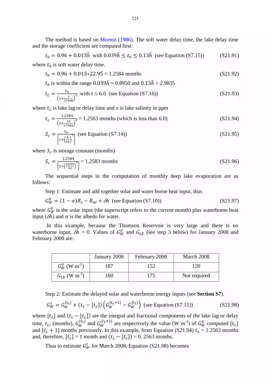
121

The method is based on Morton (1986). The soft water delay time, the lake delay time and the storage coefficient are computed first:

𝑡0 = 0.96 + 0.013ℎ� with 0.039ℎ� ≤ 𝑡0 ≤ 0.13ℎ� (see Equation (S7.15)) (S21.91)

where 𝑡0 is soft water delay time.

𝑡0 = 0.96 + 0.013×22.95 = 1.2584 months (S21.92)

𝑡0 is within the range 0.039ℎ� = 0.8950 and 0.13ℎ� = 2.9835

𝑡𝐿 = 𝑡0

�1+ 𝑠27000�

2 with 𝑡 ≤ 6.0 (see Equation (S7.16)) (S21.93)

where 𝑡𝐿 is lake lag or delay time and 𝑠 is lake salinity in ppm

𝑡𝐿 = 1.2584

�1+ 2327000�

2 = 1.2563 months (which is less than 6.0) (S21.94)

𝑆𝑐 = 𝑡0

�1+� ℎ�93�

7� (see Equation (S7.14)) (S21.95)

where 𝑆𝑐 is storage constant (months)

𝑆𝑐 = 1.2584

�1+�22.9593 �

7� = 1.2583 months (S21.96)

The sequential steps in the computation of monthly deep lake evaporation are as follows:

Step 1: Estimate and add together solar and water borne heat input, thus

𝐺𝑊0 = (1 − 𝛼)𝑅𝑠 − 𝑅𝑛𝑙 + δℎ (see Equation (S7.10)) (S21.97)

where 𝐺𝑊0 is the solar input (the superscript refers to the current month) plus waterborne heat input (δℎ) and 𝛼 is the albedo for water.

In this example, because the Thomson Reservoir is very large and there is no waterborne input, δℎ = 0. Values of 𝐺𝑊0 and 𝐺𝐿𝐸 (see step 3 below) for January 2008 and February 2008 are:

January 2008 February 2008 March 2008

𝐺𝑊0 (W m-2) 187 152 120

𝐺𝐿𝐸 (W m-2) 160 175 Not required

Step 2: Estimate the delayed solar and waterborne energy inputs (see Section S7).

𝐺𝑊𝑡 = 𝐺𝑊[𝑡𝐿] + (𝑡𝐿 − [𝑡𝐿]) �𝐺𝑊

[𝑡𝐿+1] − 𝐺𝑊[𝑡𝐿]� (see Equation (S7.11)) (S21.98)

where [𝑡𝐿] and (𝑡𝐿 − [𝑡𝐿]) are the integral and fractional components of the lake lag or delay time, 𝑡𝐿, (months), 𝐺𝑊

[𝑡𝐿] and 𝐺𝑊[𝑡𝐿+1] are respectively the value (W m-2) of 𝐺𝑊0 computed [𝑡𝐿]

and [𝑡𝐿 + 1] months previously. In this example, from Equation (S21.94) 𝑡𝐿 = 1.2563 months and, therefore, [𝑡𝐿] = 1 month and (𝑡𝐿 − [𝑡𝐿]) = 0. 2563 months.

Thus to estimate 𝐺𝑊𝑡 for March 2008, Equation (S21.98) becomes

122

𝐺𝑊𝑀𝑎𝑟08 = 𝐺𝑊[𝐹𝑒𝑏08] + (𝑡𝐿 − [𝑡𝐿]) �𝐺𝑊

[𝐽𝑎𝑛08] − 𝐺𝑊[𝐹𝑒𝑏08]� (S21.99)

𝐺𝑊𝑀𝑎𝑟08 = 152 + (0.2563)(187 − 152) = 160.71 W m-2 (S21.100)

Step 3: Compute the available and water borne energy.

𝐺𝐿𝐸 = 𝐺𝐿𝐵 + 𝐺𝑊𝑡 −𝐺𝐿𝐵0.5+𝑆𝑐


𝐺𝐿 = 0.5(𝐺𝐿𝐸 + 𝐺𝐿𝐵) (see Equation (S7.13)) (S21.102)

where 𝐺𝐿𝐵 and 𝐺𝐿𝐸 are respectively the available solar and waterborne heat energy (W m-2) at the beginning and end of the month

𝐺𝐿𝐸𝑀𝑎𝑟08 = 𝐺𝐿𝐸𝐹𝑒𝑏08 + 𝐺𝑊𝑀𝑎𝑟08−𝐺𝐿𝐸

𝐹𝑒𝑏08

0.5+𝑆𝑐 (S21.103)

𝐺𝐿𝐸𝑀𝑎𝑟08 = 175 + 160.71−1750.5+1.2583

= 166.87 W m-2 (S21.104)

𝐺𝐿𝑀𝑎𝑟08 = 0.5�𝐺𝐿𝐸𝑀𝑎𝑟08 + 𝐺𝐿𝐸𝐹𝑒𝑏08� (S21.105)

𝐺𝐿𝑀𝑎𝑟08 = 0.5(166.87 + 175) = 170.94 W m-2 (S21.106)

Step 4: Convert the available energy per month to a monthly lake evaporation rate by applying the sequence of steps set out in the worked example CRAE: Estimate actual evaporation after Equation S21.87 where

𝑅𝑇𝐶 = 𝐺𝐿𝑀𝑎𝑟08 = 170.94 W m-2 (S21.107)

These calculations yield the March 2008 lake evaporation for Thomson Reservoir as 186 mm.

123

References for Supplementary Material Abbott, M.B., Bathurst, C., Cunge, J.A., O’Connell, P.E., and Rasmussen, J.: An

introduction to the European Hydrological System - Systeme Hydrologique Europeen, SHE. 1. History and philosophy of a physically-based, distributed modelling system, Journal of Hydrology, 87, 45-59, 1986a.

Abbott, M.B., Bathurst, C., Cunge, J.A., O’Connell, P.E., and Rasmussen, J.: An introduction to the European Hydrological System - Systeme Hydrologique Europeen, SHE. 1. Structure of a physically-based, distributed modelling system, Journal of Hydrology, 87, 61-77, 1986b.

Abtew, W. and Obeysekera, J.: Lysimeter study of evapotranspiration of Cattails and comparison of three methods, Transactions American Society of Agricultural Engineers, 38, 121-129, 1995.

Adam, J.C., Clark, E.A., Lettenmaier, D.P., and Wood, E.F.: Correction of global precipitation products for orographic effects, Journal of Climate, 19, 15-38, 2006.

Al-Rawi, M.N.A.: A simple, accurate and reliable method for measuring the Sun’s elevation and orientation, Renewable Energy, 1, 231-235, 1991.

Alexandris, S., Stricevic, R., and Petkovic, S.: Comparative analysis of reference evapotranspiration from the surface of rainfed grass in central Serbia, calculated by six empirical methods against the Penman-Monteith formula, European Water, 21/22, 17-28, 2008.

Ali, S., Ghosh, N.C., and Singh, R.: Evaluating best evaporation estimate model for water surface evaporation in semi-arid India, Hydrological Processes, 22, 1093-1106, 2008.

Allen, R. G. and Brockway, C. E.: Estimating Consumptive Use on a Statewide Basis, Proceedings of the 1983 Irrigation Specialty Conference, ASCE, Jackson, Wyo., 79-89, 1983.

Allen, J.B. and Crow, F.T.: Predicting lake evaporation by performance of evaporation, ponds, pans and tanks, Transactions of the American Society of Agricultural Engineers, 14, 458-463, 1971.

Allen, R.G. and Pruitt, W.O.: Rational Use of The FAO Blaney-Criddle Formula, Journal Irrigation and Drainage Engineering, 112, 139-155, 1986.

Allen, R.G., Pereira, L.S., Raes, D., and Smith, M.: Crop evapotranspiration Guidelines for computing crop water requirements FAO Irrigation and Drainage Paper 56, Food and Agriculture Organization of the United Nations, 1998.

Allen, R.G., Pruitt, W.O., Raes, D., Smith, M., and Pereira, L.S.: Estimating evaporation from bare soil and the crop coefficient for the initial period using common soils information, Journal of Irrigation and Drainage Engineering, 131, 14-23, 2005.

Alvarez, M.V., Gonzalez-Real, M.M., Baille, A., and Molina Martinez, J.M.: A novel approach for estimating the pan coefficient of irrigation water reservoirs: Application to South Eastern Spain, Agricultural Water Management, 92, 29-40, 2007.

Amatya, D.M., Skaggs, R.G., and Gregory, J.D.: Comparison of methods for estimating REF-ET, Journal of Irrigation and Drainage Engineering, 121, 427-435, 1995.

Amer, K.H. and Hatfield, J.L.: Canopy resistance as affected by soil and meteorological factors in potato, Journal of Agronomy, 96, 978-985, 2004.

124

Anderson, M.G. and Idso, S.B.: Surface geometry and stomatal conductance effects on evaporation from aquatic macrophytes, Water Resources Research, 23, 1037-1042, 1987.

ASCE: The ASCE Standardized Reference Evapotranspiration Equation, Allen, R.G., Walter, I.A., Elliott, R., Howell, T., Itenfisu, D., and Jensen, M. (Eds), American Society of Civil Engineers, The ASCE standardized reference evapotranspiration equation, Task Committee on Standardized Reference Evapotranspiration, EWRI-American Society Civil Engineers, 59pp., 2005.

Australian Bureau of Meteorology: Australian daily evaporation, Technical Notes, National Climate Centre, Product Code IDCJCO, 2007.

Bahel, V., Srinivasan, R., and Bakhsh, H.: Solar radiation for Dhahran, Saudi Arabia, Energy, 11, 985–989, 1986.

Barton, I.J.: A parameterization of the evaporation from nonsaturated surfaces, Journal of Applied Meteorology, 18, 43-47, 1979.

Benson, R.B., Paris, M.V., Sherry, J.E., and Justus, C.G.: Estimation of daily and monthly direct, diffuse and global solar radiation from sunshine duration measurements, Solar Energy, 32, 523–535, 1984.

Berger, A., Loutre, M-F., and Tricot, C.: Insolation and Earth’s orbital periods, Journal of Geophysical Research, 90, 10341-10362, 1993.

Beven, K.: A sensitivity analysis of the Penman-Monteith actual evapotranspiration estimates, Journal of Hydrology, 44, 169-190, 1979.

Bidlake, W.R.: Evapotranspiration from a bulrush-dominated wetland in the Klamath Basin, Oregon, Journal of the American Water Resources Association, 36, 1309-1320, 2000.

Black, P.E.: Revisiting the Thornthwaite and Mather water balance, Journal of the American Water Resources Association, 43, 1604-1605, 2007.

Black, T.A.: Evapotranspiration from Douglas-fir stands exposed to soil water deficits, Water Resources Research, 15, 164-170, 1979.

Blaney, H.F.: Monthly consumptive use requirements for irrigated crops, Journal of Irrigation and Drainage Division, American Society of Civil Engineers, 85, 1-12, 1959.

Bowen, I.S.: The ratio of heat loss by conduction and by evaporation from any water surface, Physical Review, 27, 779-787, 1926.

Brezny, O., Mehta, I., and Sharma, R.K.: Studies on evapotranspiration of some aquatic weed, Weed Science, 21, 197-204, 1973.

Bristow, K.L. and Campbell, G.S.: On the relationship between incoming solar radiation and daily maximum and minimum temperature, Agricultural and Forest Meteorology, 31, 159–166, 1984.

Brown, T.C., Hobbins, M.T., and Ramírez, J.A.: Spatial distribution of water supply in the coterminous United States, Journal of the American Water Resources Association, 44, 1474-1487, 2008.

Brutsaert, W.: Evaporation into the atmosphere. Dordrecht, Holland, D. Reidel Publishing Company, 1982.

Brutsaert, W. and Stricker, H.: An advection-aridity approach to estimate actual regional evapotranspiration, Water Resources Research, 15, 443-449, 1979.

125

Burman, R.D.: Intercontinental comparison of evaporation estimates, Journal of the Irrigation and Drainage Division, 102, 109-118, 1976.

Cabral, O.M.R., Rocha, H.R., Gash, J.H.C., Ligo, M.A.V., Freitas, H.C., and Tatsch, J.D.: The energy and water balance of a Eucalyptus plantation in southeast Brazil, Journal of Hydrology, 388, 208-216, 2010.

Calder, I.R. and Neal, C.: Evaporation from saline lakes: a combination equation approach, Hydrological Sciences Journal, 29, 89-97, 1984.

Carlson, T.: An overview of the "triangle method" for estimating surface evapotranspiration and soil moisture from satellite imagery, Sensors 7, 1612-1629, doi: 10.3390/s7081612, 2007.

Chapman, T.G.: Estimation of daily potential evaporation for input to rainfall-runoff models, In Ghassemi, F., Post, D., Sivapalan, M., and Vertessy, R. (Eds), MODSIM2001: Integrating models for Natural Resources Management across Disciplines, Issues and Scales, MSSANZ 1, 293-298, 2001.

Chapman, T.G.: Estimation of evaporation in rainfall-runoff models, MODSIM 2003 International Congress on Modelling and Simulation, Townsville, Australia, 2003.

Chen, R., Ersi, K., Yang, J., Lu, S., and Zhao, W.: Validation of five global radiation models with measured daily data in China, Energy Conversion and Management, 45, 1759–1769, 2004.

Chiew, F.H.S. and Jayasuria, L.N.N.: Applicability of Morton’s complementary relationship method of estimating evapotranspiration in rainfall-runoff modelling, Conference on Agricultural Engineering, Toowoomba, The Institution of Engineers, Australia, 1990.

Chiew, F.H.S. and Leahy, C.P.: Comparison of evapotranspiration variables in evapotranspiration maps for Australia with commonly used evapotranspiration variables, Australian Journal of Water Resources, 7, 1–11, 2003.

Chiew, F.H.S. and McMahon, T.A.: The applicability of Morton’s and Penman’s evapotranspiration estimates in rainfall-runoff modelling, Water Resources Bulletin, 27, 611-620, 1991.

Chiew, F.H.S. and McMahon, T.A.: An Australian comparison of Penman potential evapotranspiration estimates and Class A evaporation pan data, Australian Journal of Soil Science, 30, 101-112, 1992.

Chiew, F.H.S. and McMahon, T.A.: Complete set of daily rainfall, potential evaporation and streamflow for twenty-eight unregulated Australian catchments, Centre for Environmental Hydrology, The University of Melbourne, 1993.

Chiew, F.H.S., Stewardson, M.J., and McMahon, T.A.: Comparison of six rainfall-runoff modelling approaches, Journal of Hydrology, 147, 1-36, 1993.

Chiew, F.H.S., Kamaladasa, N.N., Malano, H.M., and McMahon, T.A.: Penman-Monteith, FAO-24 reference crop evapotranspiration and class-A pan data in Australia, Agricultural Water Management, 28, 9-21, 1995.

Chiew, F, Wang, Q.J., McConachy, F., James, R., Wright, W, and de Hoedt, G.: Evapotranspiration maps for Australia, Proceedings of 27th Hydrology and Water Resources Symposium, Institution of Engineers, Australia, CDROM (ISBN 0-8582-5778-5), 2002.

126

Chin, D.A.: Thermodynamic consistency of potential evapotranspiration estimates in Florida, Hydrological Processes, 25, 288-301, 2011.

Christiansen, J.E.: Pan evaporation and evapotranspiration from climatic data, Journal of the Irrigation and Drainage Division, ASCE, 94, Paper 5988, 1968.

Cogley, J.G.: The albedo of water as a function of latitude, Monthly Weather Review, 107, 775-781, 1979.

Cohen, S., Ianetz, A., and Stanhill, G.: Evaporative climate changes at Bet Dagan, Israel, 1964-1998, Agricultural and Forest Meteorology, 111, 83-91, 2002.

Clulow, A.D., Everson. C.S., Mengistu, M.G., Jarmain, C., Jewitt, G.P.W., Price, J.S., and Grundling, P.-L.: Measurement and modelling of evaporation from a coastal wetland in Maputaland, South Africa, Hydrology and Earth System Sciences, 16, 3233-3247, 2012.

Crockford, R.H. and Richardson, D.P.: Partitioning of rainfall into throughfall, stemflow and interception: effect of forest type, ground cover and climate, Hydrological Processes, 14, 2903-2920, 2000.

Davenport, A.G.: Rationale for determining design wind velocities, Journal American Society of Civil Engineers, ST-86, 39-68, 1960.

Davies, J.A. and Allen, C.D.: Equilibrium, potential and actual evaporation from cropped surfaces in southern Ontario, Journal of Applied Meteorology, 12, 649-657, 1973.

de Bruin, H.A.R.: A simple model for shallow lake evaporation, Journal of Applied Meteorology, 17, 1132-1134, 1978.

de Bruin, H.A.R.: The determination of (reference crop) evapotranspiration from routine weather data, Proceedings of Technical Meeting 38, Committee for Hydrological Research TNO, Evaporation in relation to hydrology, Proceedings and Informations 28, 25-37, 1981.

de Bruin, H.A.R.: Temperature and energy balance of a water reservoir determined from standard weather data of a land station, Journal of Hydrology, 59, 261-274, 1982.

de Bruin, H.A.R.: From Penman to Makkink, Proceedings of Technical Meeting 44, Committee for Hydrological Research TNO, Hooghart, J.C. (Ed.), Evaporation and weather, Proceedings and Informations 39, 5-31, 1987.

de Bruin, H.A.R. and Holtslag, A.A.M.: A simple parameterization of the surface fluxes of sensible and latent heat during daytime compared with the Penman-Monteith concept, Journal of Applied Meteorology, 21, 1610-1621, 1982.

Dingman, S.L.: Physical Hydrology, Prentice Hall, 1992.

Donohue, R.J., Roderick, M.L. and McVicar, T.R.: Deriving consistent long-term vegetation information from AVHRR reflectance data using a cover-triangle-based framework, Remote Sensing of Environment, 112, 2938-2949, 2008.

Donohue, R.J., McVicar, T.R., and Roderick, M.L.: Climate-related changes in Australian vegetation cover as inferred from satellite observations for 1981-2006, Global Change Biology, 15, 1025-1039, 2009.

Donohue, R.J., McVicar, T.R., Li, L.T., and Roderick, M.L.: A data resource for analysing dynamics in Australian ecohydrological conditions, Austral Ecology, 35, 593-594, 2010a.

127

Donohue, R.J., McVicar, T.R., and Roderick, M.L.: Assessing the ability of potential evaporation formulations to capture the dynamics in evaporative demand within a changing climate, Journal of Hydrology, 386, 186-197, 2010b.

Doorenbos, J. and Pruitt, W.O.: Guidelines for predicting crop water requirements, FAO Irrigation and Drainage Paper 24, Food and Agriculture Organization of the United Nations, 1992.

Douglas, E.M., Jacobs, J.M., Sumner, D.M., and Ray, R.L.: A comparison of models for estimating potential evapotranspiration for Florida land cover types, Journal of Hydrology, 373, 366-376, 2009.

Drexler, J.D., Snyder, R.L., Spano, D., and Paw U, K.T.: A review of models and micrometeorological methods used to estimate wetland evapotranspiration, Hydrological Processes, 18, 2071-2101, 2004.

Droogers, P. and Allen, R.G.: Estimating reference evapotranspiration under inaccurate data conditions, Irrigation and Drainage Systems, 16, 33-45, 2002.

Dunin, F.X. and Greenwood, E.A.N.: Evaluation of the ventilated chamber for measuring evaporation from a forest, Hydrological Processes, 1, 47-62, 1986.

Dunne, T. and Leopold, L.B.: Water in Environmental Planning, W. H. Freeman and Company, New York, 1978.

Duru, J.O.: Blaney-Morin-Nigeria evapotranspiration model, Journal of Hydrology, 70, 71-83, 1984.

Edinger, J.E., Duttweiler, D.W., and Geyer, J.C.: The response of water temperature to meteorological conditions, Water Resources Research, 4, 1137-1143, 1968.

Elhaddad, A., Garcia, L.S., and Chávez, J.L.: Using a surface energy balance model to calculate spatially distributed actual evapotranspiration, Journal of Irrigation and Drainage Engineering, ASCE, 137, 17-26, 2011.

Elsawwaf, M., Willems, P., and Feyen, J.: Assessment of the sensitivity and prediction uncertainty of evaporation models applied to Nasser Lake, Egypt, Journal of Hydrology, 395, 10-22, 2010.

Federer, C. A., Vörösmarty, C., and Fekete, B.: Intercomparison of Methods for Calculating Potential Evaporation in Regional Global Water Balance Models, Water Resources Research, 32, 2315-2321, 1996.

Fennessey, N.M: Estimating average monthly lake evaporation in the Northeast United States, Journal American Water Resources Association, 36, 759-769, 2000.

Ficke, J.F.: Comparison of evaporation computation method, Pretty Lake, United States Geological Survey Professional Paper 686-A, 48 pp., 1972.

Finch, J.W.: A comparison between measured and modelled open water evaporation from a reservoir in south-east England, Hydrological Processes, 15, 2771-2778, 2001.

Finch, J.W. and Gash, J.H.C.: Application of a simple finite difference model for estimating evaporation from open water, Journal of Hydrology, 255, 253-259, 2002.

Fisher, J.B., de Biase, T.A., Qi, Y., Xu, M., and Goldstein, A.H.: Evapotranspiration models compared on a Sierra Nevada forest ecosystem, Environmental Modelling & Software, 20, 783-796, 2005.

128

Fleming, P.M., Brown, J.A.H., and Aitken, A.P.: Evaporation in Botswana and Australia, the transference of equations and techniques between continents, Hydrology and Water Resources Symposium 1989, The Institution of Engineers, Australia, National Conference Publication 89, 58-65, 1989.

Flint, A.L. and Childs, S.W.: Use of the Priestley-Taylor evaporation equation for soil water limited conditions in a small forest clearcut, Agricultural and Forest Meteorology, 56, 247-260, 1991.

Fraedrich, K., Behlau, A., Kerath, G., and Weber, G.: A simple model for estimating the evaporation from a shallow water reservoir, Tellus, 29, 428-434, 1977.

Frevert, D.K., Hill, R.W., and Braaten, B.C.: Estimation of FAO evapotranspiration coefficients, Journal of Irrigation and Drainage, ASCE, 109, 265-270, 1983.

Gash, J.H.C.: An analytical model of rainfall interception by forests, Quarterly Journal of the Royal Meteorological Society, 105, 43-55, 1979.

Gash, J.H.C., Stewart, J.B.: The evaporation from Thetford Forest during 1975, Journal of Hydrology, 35, 385-396, 1975.

Gerrits, A.W.J., Pfister, L., and Savenije, H.H.G.: Spatial and temporal variability of canopy and forest floor interception in a beech forest, Hydrological Processes, 24, 3011-3025, 2010.

Ghare, A.D., Porey, P.D., and Ingle, R.N.: Discussion of ‘Simplified estimation of reference evapotranspiration from pan evaporation data in California’ by Snyder, R.L., Orang, M., Matyac, S., and Grismer, M.E., Journal of Irrigation and Drainage Engineering, 132, 519-520, 2006.

Giles, D.G., Black, T.A., and Spittlehouse, D.L.: Determination of growing season soil water deficits on a forested slope using water balance analysis, Canadian Journal of Forest Research, 15, 107-114, 1984.

Glenn, E., Huete, A., Nagler, P, Hirschboeck, K., and Brown, P.: Integrating remote sensing and ground methods to estimate evapotranspiration, Critical Reviews in Plant Sciences, 26, 139-168, 2007.

Glenn, E. P., Nagler, P. L., and Huete, A.R.: Vegetation Index Methods for Estimating Evapotranspiration by Remote Sensing, Surveys in Geophysics, 31, 531-555, 2010.

Granger, R.J. Partitioning of energy during the snow-free season at the Wolf Creek Research Basin. In Proceedings of a Workshop held in Whitehorse, Pomeroy, J.W. and Granger, R.J. (eds), Yukon , 5-7 March, 33-43, 1998.

Granger, R.J. and Gray, D.M.: Evaporation from natural nonsaturated surfaces, Journal of Hydrology, 111, 21-29, 1989.

Granier, A., Huc., R., and Barigah, S.T.: Transpiration of natural rain forest and its dependence on climatic factors, Agricultural and Forest Meteorology, 78, 19–29, 1996.

Grant, D.R.: Comparison of evaporation measurements using different methods, Quarterly Journal of the Royal Meteorological Society, 101, 543–550, 1975.

Grayson, R.B., Argent, R.M., Nathan, R.J., McMahon, T.A., and Mein, R.G.: Hydrological Recipes - Estimation Techniques in Australian Hydrology, Cooperative Research Centre for Catchment Hydrology, Clayton, Australia, 1996.

129

Grimmond, C.S.B. and Oke, T.R.: An evapotranspiration-interception model for urban areas, Water Resources Research, 27, 1739-1755, 1991.

Guerschman, J.P., Van Dijk, A.I.J.M., Mattersdorf, G., Beringer, J., Hutley, L.B., Leuning, R., Pipunic, R.C., and Sherman, B.S.: Scaling of potential evapotranspiration with MODIS data reproduces flux observations and catchment water balance observations across Australia, Journal of Hydrology, 369, 107–119, 2009.

Harbeck, G.E.: Lake Hefner water-loss investigations, International Association Scientific Hydrology, 45, 437-443, 1958.

Harbeck, G.E.: A practical field technique for measuring reservoir evaporation utilizing mass-transfer theory, U.S. Geological Survey Professional Paper, 272-E, 1962.

Hargreaves, G.H. and Samani, Z.A.: Reference crop evapotranspiration from temperature, Applied Engineering in Agriculture, 1, 96-99, 1985.

Harmsen, E.W., Pérez, A.G., and Winter, A.: Estimating long-term average monthly evapotranspiration from pan evaporation data at seven locations in Puerto Rico, NOAA-CREST/NASA-EPSCoR Joint Symposium for Climate Studies, University of Puerto Rico – Mayaguez Campus, 7pp., 2003.

Herbst, M., Rosier, P.T.W., McNeil, D.D., and Harding, R.J.: Seasonal variability of interception evaporation from the canopy of a mixed deciduous forest, Agricultural and Forest Meteorology, 148, 1655-1667, 2008.

Hobbins, M.T., Ramírez, J.A., Brown, T.C., and Claessens, L.H.J.M.: The complementary relationship in estimation of regional evapotranspiration: The Complementary Relationship Areal Evapotranspiration and Advection-Aridity models, Water Resources Research, 37, 1367-1387, 2001a.

Hobbins, M.T., Ramírez, J.A., and Brown, T.C.: Complementary relationship in the estimation of regional evapotranspiration: An enhanced Advection-Aridity model, Water Resources Research, 37, 1388–1401, 2001b.

Hounam, C.E.: Comparison between pan and lake evaporation, World Meteorological Organisation Technical Note, 126, 52pp., 1973.

Hoy, R.D.: Pan and lake evaporation in northern Australia, Hydrology Symposium 1977, The Institution of Engineers Australia, National Conference Publication No. 77/5, 57-61, 1977.

Hoy, R.D. and Stephens, S.K.: Field study of evaporation – Analysis of data from Eucumbene, Cataract, Manton and Mundaring, A.W.R.C. Technical Paper 21, 195pp., 1977.

Hoy, R.D. and Stephens, S.K.: Field study of lake evaporation – analysis of data from phase 2 storages and summary of phase 1 and phase 2, Australian Water Resources Council, Technical Report No. 41, 1979.

Hoyt, D.V.: Percent of possible sunshine and the total cloud cover, Monthly Weather Review, 105, 648-652, 1977.

Idso, S.B.: Relative rates of evaporative water losses from open and vegetation covered water bodies, Water Resources Bulletin, 17, 46-48, 1981.

Jacobs, J.M., Mergelsberg, S.L., Lopera, A.F., and Myers, D.A.: Evapotranspiration from a wet prairie wetland under drought conditions: Paynes Prairie, Florida, USA., Wetlands, 22, 374-385, 2002.

130

Jarvis, P.G. and McNaughton, K.G.: Stomatal control of transpiration: scaling up from leaf to region, Advances in Ecological Research, 15, 1-49, 1986.

Jeffrey, S.J., Carter, J.O., Moodie, K.B., and Beswick, A.R.: Using spatial interpolation to construct a comprehensive archive of Australian climate data, Environmental Modelling and Software, 16, 309-330, 2001.

Jensen, M.E.: Estimating evaporation from water surfaces, Presentation at CSU/ARS Evapotranspiration Workshop, Fort Collins (15 March 2010), 2010.

Jensen, M.E., Burman, R.D., and Allen, R.G. (Eds): Evapotranspiration and irrigation water requirements, ASCE Manuals and Reports on Engineering Practice 70, 1990.

Jia, L., X G., Liu, S., Huang, C., Yan, Y., and Liu, G.: Regional estimation of daily to annual regional evapotranspiration with MODIS data in the Yellow River Delta wetland, Hydrology and Earth System Sciences, 13, 1775-1787, 2009.

Johnson, F., and Sharma, A.: A comparison of Australian open water body evaporation trends for current and future climates estimated from Class A evaporation pans and general circulation models, Journal of Hydrometeorology, 11, 105-121, 2010.

Jones, D.A., Wang, W., and Fawcett, R.: High-quality spatial climate data-sets for Australia, Australian Meteorological and Oceanographic Journal, 58, 233-248, 2009.

Jones, R.N., Bowler, J.M., and McMahon, T.A.: Modelling water budgets of closed lakes, western Victoria, Quaternary Australasia Papers, 11, 50-60, 1993.

Jovanovic, B., Jones, D., and Collins, D.: A high-quality monthly pan evaporation dataset for Australia, Climatic Change, 87, 517-535, 2008.

Jury, W.A. and Tanner, C.B.: Advection modification of the Priestley and Taylor evapotranspiration formula, Agronomy Journal, 67, 840-842, 1975.

Kalma, J.D., McVicar, T.R., and McCabe, M.F.: Estimating land surface evaporation: A review of methods using remotely sensed surface temperature data, Surveys in Geophysics, 29, 421-469, 2008.

Keijman, J.Q.: The estimation of the energy balance of a lake from simple weather data, Boundary-Layer Meteorology, 7, 399-407, 1974.

Keijman, J.Q. and Koopmans, R.W.R.: A comparison of several methods of estimating the evaporation of Lake Flevo, International Association of Hydrological Sciences Symposium on Hydrology of Lakes, 225-232, 1973.

Kelliher, F.M., Leuning, R. and Schulze, E.D.: Evaporation and canopy characteristics of coniferous forests and grasslands, Oecologia, 95, 153-163, 1993.

Kelliher, F.M., Leuning, R., Raupach, M.R. and Schulze, E.D.: Maximum conductances for evaporation from global vegetation types, Agricultural and Forest Meteorology, 73, 1-16, 1995.

Kirono, D.G.C., Jones, R.N., and Cleugh, H.A.: Pan-evaporation measurements and Morton-point potential evaporation estimates in Australia: are their trends the same?, International Journal of Climatology, 29, 711–718, 2009.

Klaassen, W., Bosveld, F., and de Water, E.: Water storage and evaporation as constituents of rainfall interception, Journal of Hydrology, 212-213, 36-50, 1998.

131

Kohler, M.A. and Parmele, L.H.: Generalized estimates of free-water evaporation, Water Resources Research, 3, 997-1005, 1967.

Kohler M.A., Nordenson, T.J., and Fox, W.E.: Evaporation from pans and lakes, Weather Bureau Research Paper 38, US Department of Commerce, Washington, 1955.

Komatsu, H.: Forest categorization according to dry-canopy evaporation rates in the growing season: comparison of the Priestley-Taylor coefficient values from various observation sites, Hydrological Processes, 19, 3873-3896, 2005.

Kotwicki, V.: The nature of evaporation from Lake Alexandrina, Water Down Under ’94, Adelaide, 1994.

Kumagai, T., Saitoh, T.M., Sato, Y., Morooka, T., Manfroi, O.J., Kuraji. K., and Suzuki, M.: Transpiration, canopy conductance and the decoupling coefficient of a lowland mixed dipterocarp forest in Sarawk, Borneo: dry spell effects, Journal of Hydrology, 287, 237-251, 2004.

Lavery, B., Joung, G., and Nicholls, N.: An extended high-quality historical rainfall dataset for Australia, Australian Meteorological Magazine, 46, 27-38, 1997.

Lawrence, M.G.: The relationship between relative humidity and the dewpoint temperature in moist air: a simple conversion and applications, Bulletin American Meteorological Society, 86, 225-233, 2005.

Lenters, J., Kratz, T.K., and Bowser, C.J.: Effects of climate variability on lake evaporation: results from a long-term energy budget of Sparkling Lake, northern Wisconsin (USA), Journal of Hydrology, 308, 168-195, 2005.

Linacre, E.T.: Estimating the net-radiation flux, Agricultural Meteorology, 5, 49-63, 1968.

Linacre, E.T.: Climate Data and Resources, Routledge, Boca Raton, Fla., 1992.

Linacre, E.T.: Data-sparse estimation of lake evaporation, using a simplified Penman equation, Agricultural and Forest Meteorology, 64, 237-256, 1993.

Linacre, E.T.: Estimating U.S. Class-A pan evaporation from few climate data, Water International, 19, 5-14, 1994.

Linacre, E.T., Hicks, B.B., Sainty, G.R., and Grauze, G.: The evaporation from a swamp, Agricultural Meteorology, 7, 375-386, 1970.

Lott, R.B. and Hunt, R.J.: Estimating evapotranspiration in natural and constructed wetlands, Wetlands, 21, 614-628, 2001.

Louche, A., Notton, G., Poggi, P., and Simonnot, G.: Correlations for direct normal and global horizontal irradiation on a French Mediterranean site, Solar Energy, 46, 261–266, 1991.

Lu, J., Sun, G., McNulty, S.G., and Amatya, D.M.: A comparison of six potential evapotranspiration methods for regional use in the Southeastern United States, Journal American Water Resources Association, 41, 621-633, 2005.

Magnani, F., Leonardi, S., Tognetti, R., Grace, J., and Borghetti, M.: Modelling the surface conductance of a broad-leaf canopy: effects of partial decoupling from the atmosphere, Plant Cell and Environment, 21, 867-879, 1998.

Maidment, D.R.: Handbook of Hydrology, McGraw-Hill Inc., New York, 1992.

132

Martinez-Lonano, J.A., Tena, F., Onrubia, J.E., and Rubia, J.: The historical evolution of the Ǻngström formula and its modifications: review and bibliography, Agricultural and Forest Meteorology, 33, 109-128, 1984.

McArthur, A.J.: The Penman form equations and the value of Delta: a small difference of opinion or a matter of fact?, Agricultural and Forest Meteorology, 57, 305-308, 1992.

McCullough, E.C.: Total daily radiant energy available extraterrestrially as a harmonic series in the day of the year, Arch. Met. Geoph. Biokl., Ser. B, 16, 129-143, 1968.

McCullough, E.C. and Porter, W.P.: Computing clear day solar radiation spectra for the terrestrial ecological environment, Ecology, 52, 1008-1015, 1971.

McJannet, D., Cook, F., and Burn, S.: Evaporation reduction by manipulation of surface area to volume ratios: overview, analysis and effectiveness, CSIRO: Water for a Healthy Country National Research Flagship, Urban Water Security Research Alliance Technical Report No. 8, 2008a.

McJannet, D.L., Webster. I.T., Stenson, M.P., and Sherman, B.S.: Estimating open water evaporation for the Murray-Darling Basin, A report to the Australian Government from the CSIRO Murray-Darling Basin Sustainable Yields Project, 2008b.

McJannet, D.L., Webster, I.T., and Cook, F.J.: An area-dependent wind function for estimating open water evaporation using land-based meteorological data, Environmental Modelling & Software, 31, doi:10.1016/j.envsoft.2011.11.017, 2012

McLeod, A.J. and Webster, I.T.: A heat budget method of estimating evaporation from irrigation channels, Proceedings 23rd Hydrology and Water Resources Symposium, The Institution of Engineers Australia 2, 373-379, 1996.

McNaughton, K.G. and Black, T.A.: A study of evapotranspiration from a Douglas Fir forest using the energy balance approach, Water Resources Research, 9, 1579-1590, 1973.

McNaughton, K.G. and Jarvis, P.G.: Effects of spatial scale on stomatal control of transpiration, Agricultural and Forest Meteorology, 54, 279-301, 1991.

McVicar, T.R. and Jupp, D.L.B.: Using covariates to spatially interpolate moisture availability in the Murray–Darling basin – a novel use of remotely sensed data, Remote Sensing of Environment, 79, 199–212, 2002.

McVicar, T.R., Van Niel, T.G., Li, L-T., Hutchinson, M.F., Mu, X-M., and Liu, Z-H.: Spatially distributing monthly reference evapotranspiration and pan evaporation considering topographical influences, Journal of Hydrology, 338, 196-220, 2007.

McVicar, T.R., Van Niel, T.G., Li, L.T., Roderick, M.L., Rayner, D.P. Ricciardulli, L., and Donohue, R.J.: Wind speed climatology and trends for Australia, 1975-2006: Capturing the stilling phenomenon and comparison with near-surface reanalysis output, Geophysical Research Letters, 35, L20403, doi:10.1029/2008GL035627, 2008.

McVicar, T.R., Roderick, M.L., Donohue, R.J., Li, L.T., Van Niel, T.G., Thomas, A., Grieser, J., Jhajharia, D., Himri, Y., Mahowald, N.M., Mescherskaya, A.V., Kruger, A.C., Rehman, S., and Dinpashoh, Y.: Global review and synthesis of trends in observed terrestrial near-surface wind speeds: Implications for evaporation, Journal of Hydrology, 416-417, 182-205, 2012.

Meinzer, F.C., Andrade, J.L., Goldstein, G., Holbrook, N.M., Cavelier, J., and Jackson, P.: Control of transpiration from the upper canopy of a tropical forest: the role of stomatal,

133

boundary layer and hydraulic architecture components, Plant Cell and Environment, 20, 1242–1252, 1997.

Menges, H.O., Ertekin, C, and Sonmete, M.H.: Evaluation of global solar radiation models for Konya, Turkey, Energy Conversion and Management, 47, 3149-3173, 2006.

Meyer, W.S.: Standard reference evaporation calculation for inland south eastern Australia, CSIRO Land and Water, Technical Report 35/98, 1999.

Milly, P.C.D.: A refinement of the combination equations for evaporation, Surveys in Geophysics, 12, 145-154., 1991.

Miralles, D.G., Holmes, T.R.H., De Jeu, R.A.M., Gash, J.H., Meesters, A.G.C.A., Dolman, A.J.: Global land-surface evaporation estimated from satellite-based observations, Hydrology and Earth System Sciences, 15, 453-469, 2011.

Mohamed, Y.A., Bastiaanssen, W.G.M., Savenije, H.H.G., van den Hurk, B.J.J.M., and Finlayson, C.M.: Evaporation from wetland versus open water: a theoretical explanation and an application with satellite data over the Sudd wetland, Manuscript, 2008.

Monteith, J.L.: Evaporation and environment, In Fogg, G.E. (Ed), The state and movement of water in living organisms, Symposium Society Experimental Biology, 19, 205-234., Cambridge University Press, London, 1965.

Monteith, J.L.: Evaporation and surface temperature, Quarterly Journal of the Royal Meteorological Society, 107, 1-27, 1981.

Morton, F.I.: Climatological estimates of lake evaporation, Water Resources Research, 15, 64-76, 1979.

Morton, F.I.: Operational estimates of areal evapotranspiration and their significance to the science and practice of hydrology, Journal of Hydrology, 66, 1-76, 1983a.

Morton, F.I.: Operational estimates of lake evaporation, Journal of Hydrology, 66, 77-100, 1983b.

Morton, F.I.: Practical estimates of lake evaporation, Journal of Climate & Applied Meteorology, 25, 371-387, 1986.

Morton, F.I., Richard, F., and Fogarasi, S.: Operational estimates of areal evapotranspiration and lake evaporation – Program WREVAP, NHRI Paper 24, Inland Waters Directorate, Environment Canada, Ottawa, 1985.

Mukammal, E.I. and Neumann, H.H.: Application of the Priestley-Taylor evaporation model to assess the influence of soil moisture on the evaporation from a large weighing lysimeter and class A pan, Boundary-Layer Meteorology, 12, 243-256, 1977.

Mutziger, A.J., Burt, C.M., Howes, D.J., and Allen, R.G.: Comparison of measured and FAO-56 modeled evaporation from bare soil, Journal of Irrigation and Drainage Engineering, 131, 59-72, 2005.

Muzylo, A., Llorens, P., Valente, F., Keize, J.J., Domingo, F., and Gash, J.H.C.: A review of rainfall interception modelling, Journal of Hydrology, 370, 191-206, 2009.

Myrup, L.O., Powell, T.M., Godden, D.A., and Goldman, C.R.: Climatological estimate of the average monthly energy and water budgets of Lake Tahoe, California-Nevada, Water Resources Research, 15, 1499-1508, 1979.

134

Nandagiri, L. and Kovoor, G.M.: Performance Evaluation of Reference Evapotranspiration Equations across a Range of Indian Climates, Journal of Irrigation and Drainage Engineering, 132, 238-249, 2006.

New, M., Lister, D., Hulme, M., and Makin, I.: A high-resolution data set of surface climate over global land areas, Climate Res., 21, 1-25, 2002.

Neuwirth, F.: Experiences with evaporation pans at a shallow steppe-lake in Austria, International Association of Hydrological Science ‘Hydrology of Lakes’, Helsinki, 290-297, 1973.

Nimmo, W.R.: Measurement of evaporation by pans and tanks, Australian Meteorological Magazine, 46, 17-53, 1964.

Nordenson, T.J. and Baker, D.R.: Comparative evaluation of evaporation instruments, Journal of Geophysical Research, 67, 671-679, 1962.

Oliver, H.: Irrigation and Climate, Edward Arnold Ltd., London, 250 pp., 1961.

Oudin, L., Michel, C., and Andtil, F.: Which potential evapotranspiration input for a lumped rainfall-runoff model? Part 1 – Can rainfall-runoff models effectively handle detailed potential evapotranspiration inputs?, Journal of Hydrology, 303, 275-289, 2005.

Page, J.K.: The estimation of monthly mean values of daily total short wave radiation on vertical and inclined surfaces from sunshine records for latitudes 40 N–40 S, In: Proceedings of UN Conference on New Sources of Energy, 378–90, 1961.

Paw U, K.T.: A discussion of the Penman form equations and comparisons of some equations to estimate latent energy flux density, Agricultural and Forest Meteorology, 57, 297-304, 1992.

Paw U, K.T. and Gao, W.: Applications of solutions to non-linear energy budget equations, Agricultural and Forest Meteorology, 43, 121-145, 1988.

Payne, R.E.: Albedo of sea water, Journal of Atmospheric Research, 29, 959-970, 1972.

Penman, H.L.: Natural evaporation from open water, bare soil and grass, Proceedings Royal Society London, A193, 120-145, 1948.

Penman, H.L.: Evaporation: An introductory survey, Netherlands Journal Agricultural Science, 4: 9-29, 1956.

Philip, J.R.: Evaporation and moisture and heat fields in the soil, Journal of Meteorology, 14, 354-366, 1957.

Price, J.S.: Evapotranspiration from a lakeshore Typha marsh on Lake Ontario, Aquatic Botany 48, 261-272, 1994.

Priestley, C.H.B. and Taylor, R.J.: On the assessment of surface heat flux and evaporation using large scale parameters, Monthly Weather Review, 100, 81-92, 1972.

Raupach, M.R.: Combination theory and equilibrium evaporation, Quarterly Journal of the Royal Meteorological Society, 127, 1149-1181, 2001.

Raupach, M.R., Kirby, J.M., Barrett, D.J., Briggs, P.R., Lu, H., and Zhang, H.: Balances of Water, Carbon, Nitrogen and Phosphorus in Australian Landscapes: (2) Model Formulation and Testing, CSIRO Land and Water Technical Report 41/01, 2001.

Rayner, D.: Australian synthetic daily Class A pan evaporation, Queensland Department of Natural resources and Mines Technical Report, 2005.

135

Ritchie, J.T.: Model for predicting evaporation from row crop with incomplete cover, Water Resources Research, 8, 1204-1213, 1972.

Roderick, M.L.: Estimating the diffuse component from daily and monthly measurements of global radiation, Agricultural and Forest Meteorology, 95, 169-185, 1999.

Roderick, M.L., Rotstayn, L.D., Farquhar, G.D. and Hobbins, M.T.: On the attribution of changing pan evaporation, Geophysical Research Letters 34, L17403, doi:10.1029/2007GL031166, 2007.

Roderick, M.L., Hobbins, M.T., and Farquhar, G.D.: Pan evaporation trends and the terrestrial water balance. 1. Principles and observations, Geography Compass, 3, 746-760, 2009a.

Roderick, M.L., Hobbins, M.T., and Farquhar, G.D.: Pan evaporation trends and the terrestrial water balance. 1. Energy balance and interpretation, Geography Compass, 3, 761-780, 2009b.

Rosenberry, D.O., Stannard, D.I., Winter, T.C., and Martinez, M.L.: Comparison of 13 equations for determining evapotranspiration from a prairie wetland, Cottonwood Lake Area, North Dakota, USA, Wetlands, 24, 483, 2004.

Rosenberry, D.O., Winter, T.C., Buso, D., and Likens, G.E.: Comparison of 15 evaporation methods applied to a small mountain lake in the northeastern USA, Journal of Hydrology, 340, 149-166, 2007.

Rotstayn, L.D., Roderick, M.L., and Farquhar, G.D.: A simple pan-evaporation model for analysis of climate simulation: Evaluation over Australia, Geophysical Research Letters, 33, L17715, doi:10.1029/2006GL027114, 2006.

Rutter, A.J., Kershaw, K.A., Robbins, P.C., and Morton. A.J.: A predictive model of rainfall interception in forests. I. Derivation of the model from observations in a plantation of Corsican pine, Agricultural Meteorology, 9, 367-384, 1971.

Rutter, A.J., Morton, A.J., and Robins, P.C.: A predictive model of rainfall interception in forests. II. Generalization of the model and comparison with observations in some coniferous and hardwood stands, Journal of Applied Ecology, 12, 367-380, 1975.

Sacks, L.A., Lee, T.M., and Radell, M.J.: Comparison of energy-budget evaporation losses from two morphometrically different Florida seepage lakes, Journal of Hydrology, 156, 311-334, 1994.

Salvucci, G.D.: Soil and moisture independent estimation of stage-two evaporation from potential evaporation and albedo or surface temperature, Water Resources Research, 33, 111-122, 1997.

Samani, Z.: Estimating Solar Radiation and Evapotranspiration Using Minimum Climatological Data, Journal of Irrigation and Drainage Engineering, 126, 265-278, 2000.

Saunders, R.W.: The determination of broad-band surface albedo from AVHRR visible and near-infrared radiances, International Journal of Remote Sensing, 11, 49–67, 1990.

Scozzafava, M. and Tallini, M.: Net infiltration in the Gran Sasso Massif of central Italy using the Thornthwaite water budget and curve number method, Hydrogeology Journal, 9, 461-475, 2001.

Sharma, M.L.: Evapotranspiration from an Eucalytus community, Agricultural Water Management, 8, 41-56, 1984.

136

Shaw, E.M.: Hydrology in Practice, Chapman & Hall, London, 3rd Edition, 569 pp., 1994.

Shuttleworth, W.J.: A simplified one dimensional theoretical description of the vegetation-atmosphere interaction, Boundary Layer Meteorology, 14, 3-27, 1978.

Shuttleworth, W.J.: Evaporation from Amazonian rainforest, Proceedings Royal Society London, B 233, 321-246, 1988.

Shuttleworth, W.J.: In: Maidment, D.R. (Ed.), Evaporation. McGraw-Hill, New York, pp. 4.1-4.53 (Chapter 4), 1992.

Shuttleworth, W.J. and Calder, I.R.: Has the Priestley-Taylor equation any relevance to forest evaporation?, Journal of Applied Meteorology, 18, 639-646, 1979.

Shuttleworth, W.J. and Gurney, R.J.: The theoretical relationship between foliage temperature and canopy resistance in sparse crops, Quarterly Journal Royal Meteorological Society, 116, 497-519, 1990.

Shuttleworth, W.J. and Wallace, J.S.: Evaporation from sparse crops – an energy combination theory, Quarterly Journal of the Royal Meteorological Society, 111, 839-855, 1985.

Shuttleworth, W.J. and Wallace, J.S.: Calculating the water requirements of irrigated crops in Australia using the Matt-Shuttleworth approach, Transactions of the American Society of Agricultural and Biological Engineers, 52, 1895-1906, 2009.

Silberstein, R.P., Sivapalan, M., Viney, N.R., Held, A., and Hatton, T.J.: Modelling the energy balance of a natural jarrah (Eucalyptus marginata) forest, Agricultural and Forest Meteorology, 115, 210-230, 2003.

Simpson, J.P. and Paulson, C.A.: Mid-ocean observations of atmospheric radiation, Quarterly Journal of Royal Meteorological Society, 103, 487-502, 1979.

Siriwardena, L., Finlayson, B.L. and McMahon, T.A.: The impact of land use change on catchment hydrology in large catchments: The Comet River, Central Queensland, Australia, Journal of Hydrology, 326, 199-214, 2006.

Slatyer, R.O. and McIlroy, I.C.: Practical Microclimatology, Commonwealth Scientific and Industrial Organisation, Australia, UNESCO, 1961.

Snyder. R.L., Orang, M., Matyac, S., and Grismer, M.E.: Simplified estimation of reference evapotranspiration. From pan evaporation data in California, Journal of Irrigation and Drainage Engineering, 131, 249-253, 2005.

Sobrino, J.A., Gómez, M., Jiménez-Muñoz, J.C., Olioso, A., and Chehbouni, G.: A simple algorithm to estimate evapotranspiration from DAIs data: Application to the DAISEX campaigns, Journal of Hydrology, 315, 117-125, 2005.

Souch, C., Grimmond, C.S.B., and Wolfe, C.P.: Evapotranspiration rates from wetlands with different disturbance histories: Indiana Dunes National Lakeshore, Wetlands, 18, 216-229, 1998.

Stanhill, G.: Evaporation in Israel, Bulletin of Research Council of Israel, 11G, 160-172, 1963.

Stanhill, G.: Evaporation from Lake Tiberias: an estimate by the combined water balance-mass transfer approach, Israel Journal of Earth Science, 18, 101-108, 1969.

137

Stanhill, G.: The CIMO International Evaporimeter Comparisons, World Meteorological Organisation, Geneva Publication 449, 38pp., 1976.

Stanhill, G.: Is the Class A evaporation pan still the most practical and accurate method for determining irrigation water requirements?, Agricultural and Forest Meteorology, 112, 233-236, 2002.

Stannard, D.I.: Comparison of Penman-Monteith, Shuttleworth-Wallace, and modified Priestley-Taylor Evapotranspiration models for wildland vegetation in semiarid rangeland, Water Resources Research, 29, 1379-1392, 1993.

Stewart, J.B.: Evaporation from the wet canopy of a pine forest, Water Resources Research, 13, 915-921, 1977.

Stewart, R.B. and Rouse, W.R.: A simple method for determining the evaporation from shallow lakes and ponds, Water Resources Research, 12, 623-628, 1976.

Stewart, R.B. and Rouse, W.R.: Substantiation of the Priestley and Taylor parameter alpha = 1.26 for potential evaporation in high latitudes, Journal of Applied Meteorology, 16, 649-650, 1977.

Stitger, C.J.: Solar radiation as statistically related to sunshine duration: a comment using low-latitude data, Agricultural Meteorology, 21, 173-178, 1980.

Sumner, D.M. and Jacobs, J.M.: Utility of Penman-Monteith, Priestley-Taylor, reference evapotranspiration, and pan evaporation methods to estimate pasture evapotranspiration, Journal of Hydrology, 308, 81-104, 2005.

Sweers, H.E.: A nomograph to estimate the heat-exchange coefficient at the air-water interface as a function of wind speed and temperature; a critical survey of some literature, Journal of Hydrology, 30, 375-401, 1976.

Szeicz, G., Endrödi, G., and Tajchman, S.: Aerodynamic and surface factors in evaporation, Water Resources Research, 5, 380-396, 1969.

Szilagyi, J.: Modeled areal evaporation trends over the conterminous United States, Journal of Irrigation and Drainage Engineering, 127, 196-200, 2001.

Szilagyi, J.: On the inherent asymmetric nature of the complementary relationship of evaporation, Geophysical Research Letters, 34, L02405, doi:10.1029/2006GL028708, 2007.

Szilagyi, J. and Jozsa, J.: New findings about the complementary relationship-based evaporation estimation methods, Journal of Hydrology, 354, 171-186, 2008.

Szilagyi, J., Hobbins, M.T., and Jozsa, J.: Modified Advection-Aridity model of evapotranspiration, Journal of Hydrologic Engineering, 14, 569-574, 2009.

Tang, R., Li, Z-L., and Tang, B.: An application of the T-s-VI triangle method with enhanced edges determination for evapotranspiration estimation from MODIS data in and semi-arid regions: Implementation and validation, Remote Sensing of Environment, 114, 540-551, 2010.

Teklehaimont, Z. and Jarvis, P.G.: Direct measurement of evaporation of intercepted water from forest canopies, Journal of Applied Ecology, 28, 603-618, 1991.

Thom, A.S., Thony, J.-L., and Vauclin, M,: On the proper employment of evaporation pans and atmometers in estimating potential transpiration, Quarterly Journal of the Royal Meteorological Society, 107, 711-736, 1981.

138

Thornthwaite, C.W.: An approach toward a rational classification of climate, Geographical Review, 38, 55-94, 1948.

Thornthwaite, C.W. and Mather, J.R.: Instructions and Tables for the Computing Potential Evapotranspiration and the Water Balance, Drexel Institute of Technology Publications in Climatology 10, 185-311, 1957.

Tiris, M., Tiris, C., and Erdalli, Y.: Water heating systems by solar energy, Marmara Research Centre, Institute of Energy Systems and Environmental Research, NATO TU-COATING, Gebze, Kocaeli, Turkey [in Turkish], 1997.

Trajković, S. and Kolakovic. S.: Evaluation of reference evapotranspiration equations under humid conditions, Water Resources Management, 23, 3057-3067, 2009.

Trajković, S. and Kolakovic, S.: Comparison of simplified pan-based equations for estimating reference evapotranspiration, Journal of Irrigation and Drainage Engineering 136, 137-140, 2010.

Trajković, S. and Stojnić, V.: Effect of wind speed on accuracy of Turc method in a humid climate, Facta Universitstis, Architecture and Civil Engineering, 5, 107-113, 2007.

Turc, L.: Le bilan d’eau des sols. Relations entre les précipitations, l’evaporation et l’écoulement, Annual Agronomy, 5, 491-596, 1954.

Turc, L.: Le bilan d’eau des sols. Relations entre les précipitations, l’evaporation et l’écoulement, Annual Agronomy, 6, 5-131, 1955.

Turc, L.: Estimation of irrigation water requirements, potential evapotranspiration: A simple climatic formula evolved up to date (in French), Annual Agronomy, 12, 13–49, 1961.

Ulgen, K. and Hepbasli. A.: Solar radiation models. Part 1: a review, Energy Sources, 26, 507-520, 2004.

Valiantzas, J.D.: Simplified versions for the Penman evaporation equation using routine weather data, Journal of Hydrology, 331, 690-702, 2006.

van Bavel, C.H.M.: Potential evaporation: The combination concept and its experimental verification, Water Resources Research, 2, 455-467, 1966.

van Dijk, M.H.: Reduction in evaporation due to the bird screen used in the Australian class-A pan evaporation network, Australian Meteorological Magazine, 33, 181-183., 1985.

Vardavas, I.M.: Modelling the seasonal variation of net all-wave radiation flux and evaporation in a tropical wet-dry region, Ecological Modelling, 39, 247-268, 1987.

Vardavas, I.M. and Fountoulakis, A.: Estimation of lake evaporation from standard meteorological measurements: application to four Australian lakes in different climatic regions, Ecological Modelling, 84, 139-150, 1996.

Wallace, J. and McJannet, D.: Processes controlling transpiration in the rainforests of north Queensland, Australia, Journal of Hydrology, 384, 107-117, 2010.

Wang, Q.J., Chiew, F.H.S., McConachy, F.L.N., James, R., de Hoedt, G.C., and Wright, W.J.: Climatic Atlas of Australia Evapotranspiration Bureau of Meteorology, Commonwealth of Australia, 2001.

Watts, P.J. and Hancock, N.H.: Evaporation and potential evaporation – A practical approach for agricultural engineers, Conference on Agricultural Engineering, Bundaberg, The Institution of Engineers, Australia, National Conference Publication 84, 290-297, 1984.

139

Webb, E.K.: A pan-lake evaporation relationship, Journal of Hydrology, 4, 1-11, 1966.

Weeks, W.D.: Evaporation: a case study using data from a lake in Eastern Queensland, Hydrology and Water resources Symposium, Melbourne, The Institution of Engineers, Australia, National Conference Publication 82, 189-193, 1982.

Weiβ, M. and Menzel, L.: A global comparison of four potential evapotranspiration equations and their relevance to stream flow modelling in semi-arid environments, Advances in Geoscience, 18, 15-23, 2008.

Wessel, D.A. and Rouse, W.R.: Modelling evaporation from wetland tundra, Boundary-Layer Meteorology, 68, 109-130, 1994.

Wieringa, J.: Roughness-dependent geographical interpolation of surface wind speed averages, Quarterly Journal of Royal Meteorological Society, 112, 867-889, 1986.

Winter, T.C.: Uncertainties in estimating the water balance of lakes, Water Resources Bulletin, 17: 82 – 115, 1981.

Winter, T.C. and Rosenberry, D.O.: Evaluation of 11 equations for determining evaporation for a small lake in the north central United States, Water Resources Research, 31, 983-993, 1995.

Xu, C.-Y. and Chen, D.: Comparison of seven models for estimation of evapotranspiration and groundwater recharge using lysimeter measurement data in Germany, Hydrological Processes, 19, 3717-3734, 2005.

Xu, C.-Y. and Singh, V.P.: Evaluation and generalisation of temperature-based methods for calculating evaporation, Hydrological Processes, 15, 305-319, 2001.

Xu, C.-Y. and Singh, V.P.: Cross comparison of empirical equations for calculating potential evapotranspiration with data from Switzerland, Water Resources Management, 16, 197-219, 2002.

Yang, K., Koike, T., and Ye, B.: Improving estimation of hourly, daily, and monthly solar radiation by importing global data sets, Agricultural and Forest Meteorology, 137, 43–55, 2006.

Yang, J. and Wang, Y.: Estimating evapotranspiration fraction by modeling two-dimensional space of NDVI/albedo and day-night surface temperature difference: A comparative study, Advances in Water Resources, 34, 512-518, 2011.

Yin, Z.-Y. and Brook, G.A.: Evapotranspiration in the Okefenokee Swamp watershed: a comparison of temperature-based and water balance methods, Journal of Hydrology, 131, 293-312, 1992.

Young, A.A.: Some recent evaporation investigations, Transactions of the American Geophysical Union, 28, 279-284, 1947.

Zhang, L., Dawes, W.R., and Walker G. R.: Response of mean annual evapotranspiration to vegetation changes at catchment scale, Water Resources Research, 37, 701-708, 2001.

140

Table S1 Values of specific constants

Constant Symbol Value Reference Atmospheric pressure 𝑝 101.3 �293−0.0065𝐸𝑙𝑒𝑣

293�5.26

kPa* Dingman (1992, p. 224)

Density of water 𝜌𝑤 997.9 kg m-3 at 20°C Dingman (1992, p. 542)

Mean air density 𝜌𝑎 1.20 kg m-3 at 20°C Shaw (1994, p. 6) Emissivity of water 𝜀𝑤 0.95 Dingman (1992, p. 583) Surface emissivity 𝜀𝑠 0.92 (adopted by Morton) Morton (1983b, p. 64) Specific heat of water 𝑐𝑤 4.19 kJ kg-1 °C-1 Maidment (1992, p. 7.23)

Morton (1979, p.72) Specific heat of air 𝑐𝑎 1013 J kg-1 K-1 Allen et al. (1998,

Equation 8); McJannet et al. (2008, page 43)

Latent heat of vaporization

𝜆 2.45 MJ kg-1 at 20°C 28.5 W days kg-1

Dingman (1992, p. 547) Allen et al. (1998, p. 31) Morton (1983b, p. 65)

Psychrometric constant 𝛾 𝛾 = 0.00163 𝑝𝜆 kPa°C-1 Dingman (1992, p. 225)

Stefan-Boltzmann constant

𝜎 4.90 × 10−9 MJ m-2 day-1 K-4 5.67 × 10−8 W m-2 K-4

Dingman (1992, p. 582) Morton (1983a, p.64)

von Kármán constant 𝑘 0.41 Szeicz et al., 1969) p. 380)

* 𝐸𝑙𝑒𝑣 is elevation (m)

141

Table S2 Roughness height, aerodynamic and surface resistance of typical surfaces

Surface Location Height of surface

condition (m)

Zero-plane displacement

(m)

Roughness length

(m)

Aerodynamic resistance, 𝑟𝑎,

(s m-1)

Average surface resistance, 𝑟𝑠,

(s m-1) Open sea, fetch >5 km 0.0002 o see Section S4 Open water 0.01 n 0.001 n 0 n Open flat terrain: grass 0.03 o Desert 0.001 e 0.1 c 0.05 c 200 e Semi-desert 0.5 c 0.1 c Arid land 250 j Cultivation 0.005 e 91 f Hypothetical reference crop 0.12 a 104 a 70 a Well watered production crops 50 j Short grass 0.2 c 0.02 c Tall grass 1 c 0.1 c Low crops 0.10 o High crops 0.25 o Grassland Based on 7 sites in

northern hemisphere

0.5* e, g (0.05 – 0.85)

0.5e

0.01 e, g

37 e, g (14 - 71)

40 e, g (5 – 143)

125 Uncut lucerne 1.0 n 0.1 n 22 n 60 n Evergreen shrub 1 c 0.1 c Deciduous shrub 1 c 0.1 c Parkland, bushes 0.5 o Non-forest wetland 0.3 e 152 e Savannah/xeric shrub 8.0 e 189 e Coniferous forest Based on 8

references world-wide

8 e, g (5 – 20)

25

7 e, g (5 – 14)

50 e, g (30 - 125)

189 Evergreen needleleaf forest 15 c 1.0 c

142

Deciduous needleleaf forest 20 c 1.0 c Beech Northern

Apennines, Italy 200 i

Evergreen broadleaf forest 20 c 2.0 c Deciduous broadleaf forest 15 c 0.8 c Eucalyptus plantation São Paulo State,

Brazil 12-21 b summer 19±14 b

winter 9±2 summer 19±14 b winter 167±292

Eucalyptus maculata Kioloa State Forest,NSW,

Australia

60 d

Eucalyptus forest Collie, Western Australia

5 l 50 l

Lower montane rainforest Nth Q’ld, Australia 25 & 32 m summer 71 & 163 m

winter 56 & 119 Pristine lowland rain forest Nth Q’ld, Australia 27 m summer 171 m

winter 115 Upper montane cloud rainforest

Nth Q’ld, Australia 8 m summer 317 m winter 160

Mixed woodland 20 c 0.8 c Tropical rainforest French Guiana ~28 d 140 – 170 d Tropical trees Panama 250 – 500 k Lowland mixed dipterocarp forest

Sarawak, Borneo 50 h 10 h 84 h

Regular large obstacle coverage (suburb, forest)

1.0 o

a: Allen et al. (1998, page 23), b: Cabral et al. (2010), c: Douglas et al. (2009), d: Dunin and Greenwood (1986, page 51), e: Federer et al. (1996), f: Granier et al. (1996), g: Kelliher et al.(1993), h: Kumagai et al. (2004), i: Magnani et al. (1998, page 870), j: McNaughton and Jarvis (1991), k: Meinzer et al. (1997), l: Sharma (1984, page 49), m : Wallace & McJannet (2010), n: Watt & Hancock (1984), o: Wieringa (1986, Table 1) based on Davenport (1960) *Value is median of a range shown in parenthesis # clonal Eucalyptus grandis × Eucalyptus urophylla

143

Table S3 Albedo values

Surface Albedo, α Reference Water* 0.08 Maidment (1992) Desert (bare ground) 0.30 McVicar et al. (2007) Semi-desert 0.25 Douglas et al. (2009) Tundra 0.20 Douglas et al. (2009) Short grass 0.26 Watts & Hancock (1984) Pasture (short grass) 0.26 McVicar et al. (2007), Douglas et al. (2009) Reference (short) crop 0.23 Allen et al. (1998, page 51) Long grass (1 m) 0.16 Watts & Hancock (1984) Irrigated crop 0.18 Douglas et al. (2009) Crop/mixed farming 0.20 Douglas et al. (2009) Evergreen shrub 0.10 Douglas et al. (2009) Deciduous shrub 0.20 Douglas et al. (2009) Sparse forest 0.18 McVicar et al. (2007) Rain forest 0.15 Dingman (1992) Eucalypts 0.20 Dingman (1992) Evergreen needleleaf forest 0.10 Douglas et al. (2009) Deciduous needleleaf forest 0.20 Douglas et al. (2009) Evergreen broadleaf forest 0.15 Douglas et al. (2009) Deciduous broadleaf forest 0.20 Douglas et al. (2009) Forest (mixed woodland) 0.15 McVicar et al. (2007), Douglas et al. (2009) Urban area 0.25 McVicar et al. (2007) * Based on Cogley (1979), Jensen (2010, Table 1) provides a table of albedo values for water. Jensen’s table shows that albedo for water has a seasonal pattern being high in winter and low in summer and increases from an average value of 0.065 at the equator to values varying from 0.11 to 0.36 at 60° – 70°N latitude.

144

Table S4 Median, 10th and 90th percentile monthly evaporation based on data recorded at the 68 Australian AWSs for three Penman wind functions, and for FAO-56

Reference Crop and Priestley-Taylor algorithms expressed as a percentage of the Penman (1948) median estimate

Parameter Penman FAO-56

Reference Crop

Priestley-Taylor

Penman (1948) wind

function

Penman (1956) wind

function

Linacre (1993)

Median 100% -9.9% -15.8% -26.4% -17.1% 10th percentile -63.0% -67.5% -72.0% -74.3% -75.7% 90th percentile 57.4% 45.5% 33.4% 22.3% 29.2%

Table S5 Guideline for defining shallow and deep lakes and the methods to estimate lake evaporation

Shallow lake Average

depth (m) Deep lake Average

depth (m)

Morton recommendations Morton CRWE Morton CRLE

Seasonal heat storage changes (Morton, 1983b, page 84) and water advection are not important

undefined For depths less than 1.5 m use CRWE (Morton, 1986, page 385)

1.5

Deep lakes are considered shallow if one is interested only in annual or mean annual evaporation (Morton, 1983b, page 84)

undefined Seasonal heat storage changes and water advection are important

undefined

Recommendations of other authors Shallow lake without seasonal heat storage

analysis Deep lake

Sacks et al (1994, Abstract) 3 Vardavas & Fountoulakis (1996)

3 – 23

Penman equation can be applied without adjusting for heat storage Monteith (1981, page 9)

less than “…a

metre or so…”

Kohler & Parmele (1967) undefined

de Bruin (1978, Section 2) 3 Shallow lake with seasonal heat storage

analysis

McJannet et al. (2008b) 1 – 6 McJannet et al. (2008b) 25 - 30 Finch & Gash (2002) 10 Finch & Gash (2002) 10 Finch (2001) 10 Fennessey (2000) 2 Sacks et al (1994, page 312) < 5 Fraedrich et al. (1977, Section 6) 8 Stewart & Rouse (1976, page 624) 0.6 Keijman and Koopmans (1973) 3.0

145

Table S6 Mean monthly screened Class-A evaporation pan coefficients for estimating Penman open-water evaporation (1956 wind function) at 68 Australian locations

For each station, the second row of values specifies the number of months used to compute the mean monthly pan coefficients. Asterisk denotes high quality Class-A evaporation pan. nd is no data

BOM ref. Station name Lat °S Long

°E Jan Feb Mar Apr May Jun Jul Aug Sep Oct Nov Dec Year

2012 Halls Creek Airport* 18.23 127.66 0.735 0.880 0.753 0.696 0.702 0.711 0.702 0.696 0.671 nd 0.709 0.697 0.723 3 2 2 3 2 2 2 1 1 0 1 1

3003 Broome Airport* 17.95 122.24 0.822 0.842 0.866 0.816 0.742 0.743 0.768 0.788 0.859 0.897 0.882 0.837 0.822 9 12 7 13 16 14 14 14 16 15 16 11

7178 Paraburdoo 23.20 117.67 0.607 0.571 0.591 0.614 0.564 0.654 0.594 0.644 0.635 0.587 0.608 0.591 0.605 2 1 2 1 3 3 1 2 3 3 3 2

9021 Perth Airport* 31.93 115.98 0.825 0.821 0.782 0.818 0.827 0.850 0.915 0.984 0.979 0.960 0.903 0.862 0.877 16 16 16 16 16 15 15 16 15 15 16 16

9034 Perth Reg. Office* 31.96 115.87 0.912 0.866 0.837 0.837 0.818 0.807 0.869 0.931 0.942 0.966 0.942 0.945 0.889 14 11 11 11 13 11 10 11 11 9 12 12

9538 Dwellingup 32.71 116.06 0.880 0.867 0.864 0.921 0.813 0.789 0.748 0.912 0.933 1.028 0.963 0.923 0.887 10 11 13 13 9 11 9 6 9 12 14 12

9592 Permberton 34.45 116.04 0.950 0.941 0.883 0.920 0.981 0.890 nd nd 0.892 0.980 0.983 0.962 0.938 3 4 2 2 1 1 0 0 1 1 1 2

9741 Albany Airport* 34.94 117.80 0.827 0.822 0.809 0.856 0.859 0.830 0.882 0.938 0.970 0.987 0.917 0.856 0.879 16 15 12 15 17 16 15 17 13 15 18 15

13017 Giles Met. Office* 25.03 128.30 0.650 0.656 0.650 0.686 0.727 0.765 0.755 0.747 0.718 0.694 0.678 0.659 0.699 28 26 25 27 28 30 29 28 27 28 27 28

14015 Darwin Airport* 12.42 130.89 0.775 0.771 0.866 0.855 0.779 0.744 0.766 0.812 0.836 0.853 0.838 0.779 0.806 10 12 13 25 24 29 26 29 30 25 17 16

14198 Jabiru Airport 12.66 132.89 0.842 0.856 0.827 0.812 0.766 0.709 0.734 0.740 0.732 0.773 0.788 0.848 0.786 2 3 4 3 6 4 5 5 7 7 4 2

14508 Gove Airport* 12.27 136.82 0.859 0.831 0.899 0.889 0.888 0.863 0.889 0.921 0.935 0.944 0.922 0.864 0.892 18 16 17 19 17 19 19 20 21 22 15 18

146

14513 Wallaby Beach 12.19 136.71 nd 0.773 nd 0.846 0.862 0.811 0.751 0.873 0.873 0.920 0.890 0.782 0.838 0 1 0 3 3 3 3 3 5 5 4 3

14612 Larrimah 15.57 133.21 0.756 0.878 0.850 0.780 0.792 0.739 0.793 0.798 0.756 0.709 0.697 0.577 0.760 4 3 4 3 1 3 2 2 6 1 3 3

14703 Centre Island 15.74 136.82 nd nd 0.825 0.912 0.816 0.872 0.905 1.060 0.923 0.975 0.870 0.950 0.911 0 0 1 2 1 2 2 1 2 3 2 2

14704 McArthur River Mine 16.44 136.08 0.700 0.721 0.773 0.734 0.694 0.666 0.671 0.701 0.703 0.688 0.700 0.660 0.701 4 9 6 4 4 9 5 7 4 4 5 4

15135 Tennant Creek Airport* 19.64 134.18 0.644 0.667 0.632 0.601 0.623 0.648 0.657 0.649 0.627 0.632 0.633 0.646 0.638

24 21 27 28 30 29 28 27 28 28 29 24

15590 Alice Springs Airport* 23.80 133.89 0.668 0.669 0.657 0.690 0.737 0.781 0.783 0.756 0.724 0.712 0.684 0.675 0.711 24 27 25 21 26 24 25 25 28 26 26 24

15666 Rabbit Flat 20.18 130.01 0.721 0.789 0.765 0.764 0.779 0.797 0.762 0.761 0.731 0.756 0.715 0.808 0.762 4 8 7 7 7 6 6 8 7 9 7 3

16001 Woomera Aerodrome* 31.16 136.81 0.695 0.687 0.691 0.715 0.731 0.790 0.788 0.777 0.766 0.759 0.725 0.711 0.736 24 28 28 28 28 25 27 30 25 28 27 29

17043 Oodnadatta Airport 27.56 135.45 0.630 0.633 0.652 0.669 0.713 0.754 0.750 0.762 0.739 0.744 0.656 0.636 0.695 5 5 5 4 5 6 5 4 4 3 5 4

18012 Ceduna AMO* 32.13 133.70 0.828 0.816 0.793 0.773 0.781 0.834 0.831 0.848 0.841 0.835 0.823 0.821 0.819 23 27 28 29 29 28 29 28 27 28 28 29

23034 Adelaide Airport 34.95 138.52 0.827 0.808 0.789 0.786 0.800 0.833 0.858 0.866 0.890 0.886 0.862 0.831 0.836 27 24 21 25 22 21 20 22 23 23 25 23

23090 Adelaide (Kent Town)* 34.92 138.62 0.905 0.895 0.922 0.890 0.912 0.925 0.937 0.979 0.969 0.995 0.938 0.920 0.932

10 10 9 8 8 9 9 9 9 9 9 9

23321 Nuriootpa Comparison* 34.48 139.00 0.803 0.791 0.787 0.844 0.887 0.925 0.992 0.971 0.980 0.935 0.857 0.815 0.882

19 20 18 16 20 19 18 19 18 19 16 20

23373 Nuriootpa Viticultural* 34.48 139.01 0.804 0.783 0.780 0.820 0.814 0.908 0.924 0.944 1.043 0.947 0.880 0.836 0.874

9 8 4 6 7 5 5 5 5 9 7 6

24024 Loxton Res. Centre 34.44 140.60 0.785 0.790 0.797 0.849 0.858 0.899 0.940 0.929 0.933 0.892 0.834 0.804 0.859 18 18 24 21 21 22 21 18 22 16 20 18

147

26021 Mount Gambier Aero* 37.75 140.77 0.920 0.907 0.876 0.918 0.949 1.013 1.031 1.024 1.039 1.044 0.991 0.945 0.972 31 30 29 30 28 29 28 28 30 30 27 30

27045 Weipa Aero* 12.68 141.92 0.774 0.838 0.861 0.890 0.844 0.779 0.788 0.794 0.823 0.836 0.856 0.831 0.826 4 5 3 9 14 15 13 16 10 13 8 8

29126 Mount Isa Mine 20.74 139.48 0.689 0.720 0.679 0.674 0.662 0.705 0.710 0.705 0.674 0.664 0.674 0.686 0.687 11 10 10 10 10 11 11 9 11 12 12 3

29127 Mount Isa Aero* 20.68 139.49 0.745 0.752 0.729 0.706 0.726 0.736 0.749 0.745 0.723 0.709 0.718 0.727 0.730 23 20 26 26 28 29 27 29 28 27 21 21

31011 Cairns Aero* 16.87 145.75 0.851 0.835 0.858 0.873 0.838 0.835 0.831 0.857 0.847 0.850 0.835 0.832 0.845 12 10 11 16 22 24 24 24 25 26 22 19

32040 Townsville Aero* 19.25 146.77 0.824 0.821 0.812 0.773 0.771 0.762 0.777 0.794 0.809 0.814 0.812 0.827 0.800 18 11 22 24 24 26 28 27 28 25 22 16

40223 Brisbane Aero 27.42 153.11 0.848 0.822 0.830 0.836 0.858 0.857 0.860 0.844 0.859 0.848 0.845 0.841 0.846 11 8 9 11 14 13 14 13 14 12 13 11

40428 Brian Pastures* 25.66 151.75 0.773 0.794 0.786 0.772 0.752 0.738 0.755 0.787 0.806 0.813 0.806 0.772 0.779 22 22 18 22 24 21 24 18 22 21 21 19

40842 Brisbane Aero 27.39 153.13 0.857 0.856 0.847 0.858 0.856 0.849 0.856 0.885 0.880 0.863 0.877 0.844 0.861 8 6 9 9 9 6 10 9 9 10 7 9

48027 Cobar Aero* 31.48 145.83 0.736 0.727 0.725 0.765 0.802 0.863 0.882 0.873 0.843 0.815 0.768 0.732 0.794 26 28 28 26 23 25 26 25 28 25 28 24

53048 Moree Comparison* 29.48 149.84 0.809 0.822 0.795 0.813 0.846 0.878 0.915 0.946 0.899 0.866 0.843 0.811 0.854 16 15 17 16 15 14 14 15 15 16 15 15

53115 Moree Aero* 29.49 149.85 0.791 0.783 0.786 0.777 0.797 0.862 0.886 0.883 0.867 0.838 0.811 0.788 0.822 9 10 12 13 14 13 12 15 14 14 12 14

55024 Gunnedah Res. Centre* 31.03 150.27 0.713 0.687 0.708 0.675 0.667 0.649 0.558 nd nd nd 0.763 0.710 0.681

1 2 3 3 1 3 1 0 0 0 3 3

55054 Tamworth Airport 31.09 150.85 0.806 0.795 0.809 0.802 0.858 0.904 0.912 0.962 0.896 0.876 0.863 0.830 0.859 11 10 12 12 12 14 12 9 10 11 9 10

56018 Inverell Res. Centre 29.78 151.08 0.873 0.857 0.837 0.871 0.810 0.783 0.799 0.888 0.908 0.906 0.921 0.879 0.861 8 8 6 7 10 9 10 11 11 10 11 8

148

59040 Coffs Harbour MO* 30.31 153.12 0.839 0.850 0.835 0.838 0.842 0.827 0.844 0.865 0.890 0.889 0.869 0.886 0.856 19 20 15 24 18 21 23 25 27 28 23 21

61078 Williamtown RAAF* 32.79 151.84 0.810 0.805 0.836 0.819 0.820 0.770 0.808 0.848 0.858 0.839 0.829 0.816 0.821 25 23 23 22 24 20 25 25 26 26 24 25

61089 Scone SCS* 32.06 150.93 0.862 0.853 0.841 0.870 0.879 0.895 0.908 0.933 0.953 0.937 0.891 0.851 0.889 12 13 14 13 14 14 13 15 14 12 13 12

66037 Sydney Airport AMO* 33.95 151.17 0.835 0.835 0.827 0.826 0.846 0.805 0.828 0.847 0.862 0.873 0.857 0.842 0.840

27 22 28 23 19 26 25 26 24 22 26 26

67033 Richmond RAAF 33.60 150.78 0.839 0.837 0.846 0.842 0.899 0.880 0.869 0.850 0.849 0.848 0.854 0.825 0.853 15 12 15 13 16 15 13 14 14 14 15 13

68076 Nowra RAN Air Station 34.94 150.55 0.783 0.774 0.796 0.764 0.735 0.685 0.771 0.786 0.790 0.784 0.789 0.785 0.770

15 15 19 17 16 17 17 15 13 15 17 13

70014 Canberra Airport Comparison* 35.30 149.20 0.785 0.791 0.770 0.801 0.820 0.849 0.881 0.879 0.873 0.883 0.852 0.811 0.833

30 28 28 30 29 29 29 27 28 31 28 29

70015 Canberra Forestry 35.30 149.10 nd nd 0.677 0.812 0.860 0.973 0.943 0.994 0.933 nd nd nd 0.885 0 0 1 1 1 1 1 1 1 0 0 0

72060 Khancoban SMHEA 36.23 148.14 0.869 0.867 0.867 0.958 1.022 1.221 1.227 1.164 1.040 1.028 0.949 0.873 1.007 13 12 14 14 11 14 12 13 12 13 13 12

72150 Wagga Wagga AMO* 35.16 147.46 0.815 0.813 0.810 0.865 0.944 0.984 1.069 1.097 1.053 0.988 0.893 0.843 0.931 24 25 23 21 23 22 22 22 24 22 20 23

76031 Mildura Airport* 34.24 142.09 0.793 0.785 0.785 0.819 0.840 0.882 0.921 0.925 0.889 0.864 0.838 0.811 0.846 19 21 20 17 19 19 19 20 20 21 20 19

82039 Rutherglen Research* 36.10 146.51 0.821 0.819 0.806 0.862 0.897 0.904 0.989 0.993 1.025 1.056 0.919 0.804 0.908 16 16 17 13 15 12 16 11 13 9 14 13

85072 East Sale Airport* 38.12 147.13 0.887 0.872 0.879 0.911 0.912 0.900 0.913 0.966 0.954 0.987 0.935 0.903 0.918 25 26 26 26 28 25 29 26 29 23 25 27

85103 Yallourn SEC 38.19 146.33 0.885 0.820 0.917 0.935 1.070 0.914 0.959 1.007 1.101 1.029 1.033 0.940 0.968 7 6 7 7 2 4 4 7 2 4 2 2

86282 Melbourne Airport 37.67 144.83 0.835 0.816 0.799 0.795 0.847 0.868 0.872 0.892 0.859 0.887 0.895 0.838 0.850 9 9 9 9 9 10 8 8 10 11 11 11

149

87031 Laverton RAAF 37.86 144.76 0.812 0.789 0.765 0.771 0.788 0.846 0.881 0.880 0.907 0.896 0.864 0.825 0.835 16 20 20 21 20 19 20 17 17 15 19 18

88023 Lake Eildon* 37.23 145.91 1.015 1.010 1.034 1.139 1.281 1.444 1.546 1.405 1.281 1.229 1.145 1.028 1.213 26 26 22 19 22 24 20 23 24 22 19 23

90103 Hamilton Res. Station 37.83 142.06 0.784 0.725 0.692 0.739 0.713 0.681 0.717 0.776 0.862 0.935 0.907 0.841 0.781 15 14 9 11 7 7 11 9 12 9 9 12

91104 Launceston Airport Companion* 41.54 147.20 0.880 0.882 0.858 0.908 0.967 0.961 1.062 1.110 1.079 1.043 0.979 0.893 0.968

20 20 20 20 18 15 15 19 18 22 19 19

91219 Scottsdale 41.17 147.49 1.008 1.024 1.009 1.065 1.007 0.936 0.952 1.062 1.105 1.137 1.101 1.027 1.036 24 22 17 14 15 15 17 17 16 18 21 24

92038 Swansea Post Office 42.12 148.07 0.903 0.903 0.916 0.987 1.085 0.982 0.969 1.010 1.036 1.049 0.961 0.941 0.979 2 2 2 2 2 2 2 2 2 2 2 1

94008 Hobart Airport 42.83 147.50 0.888 0.897 0.889 0.879 0.863 0.916 0.913 0.970 0.987 0.978 0.950 0.912 0.920 19 22 20 20 20 21 21 22 21 21 20 19

94029 Hobart (Ellerslie Road) 42.89 147.33 0.972 0.932 0.941 0.936 0.944 0.993 0.991 0.974 1.022 1.079 1.007 0.968 0.980

15 16 16 15 15 16 13 15 14 15 15 14

94069 Grove (Comparison)* 42.98 147.08 0.873 0.854 0.864 0.858 0.823 0.855 0.876 0.852 0.926 0.949 0.945 0.920 0.883 18 20 21 21 16 18 13 14 19 20 18 20

96033 Liawenee 41.90 146.67 1.057 nd 1.075 nd nd nd nd nd nd nd 1.132 1.068 1.083 3 0 1 0 0 0 0 0 0 0 2 2

97053 Strathgordon Village* 42.77 146.05 0.973 0.955 0.947 0.870 0.946 0.765 0.708 0.748 0.890 0.989 1.023 0.947 0.897 6 7 7 4 4 7 4 8 6 5 8 6

150

Table S7 Comparison of equations to estimate evaporation from a lake covered with vegetation

(Adv. and Disadv. are abbreviations for advantage and disadvantage, respectively.)

Reference Application Penman (Section 2.1.1)

Penman-Monteith (Section 2.1.2)

Weighted Penman-Monteith

(Equation S5.30)

Shuttleworth-Wallace

(Equation S5.22)

Priestley-Taylor (Section 2.1.3)

Wessel & Rouse (1994) Table III

Wetland tundra Adv: accurate if 𝑟𝑠 is available Disadv: inadequate for complex surfaces

Adv: handle any surfaces Weight components by surface area

Disadv: Cannot model area with no canopy. Not recommended

Bowen Ratio 0.75 (1.21)# 1.10 (1.41) 1.35 (1.65) Abtew & Obeysekera (1995) Figures 7 to 9

South Florida The two coefficients in the wind function were found by calibration

Monteith (1965) 𝑟𝑎 from Equation S5.3. 𝑟𝑠 varied from 25 s m-1 during high ET season and 90 s m-1 for rest of year.

α = 1.18 by calibration

Lysimeter within wetland complex

P=0.03+1.01Meas (see = 0.57 mm day-1)

PM=1.17+0.75Meas (see = 0.39 mm day-1)

PT=1.15 +070Meas (see = 0.53 mm day-1)

Souch et al. (1998) Table 3

Indiana, USA Undisturbed site

Penman modified by Shuttleworth (1992)

𝑟𝑎 from Shuttleworth (1992, Equation 4.2.25); 𝑟𝑠 = 0 for standing water & 𝑟𝑠 = 5 s m-1 for vegetation

Assumed vapour pressure deficits depressed, α = 1

Eddy correlation

1.03 (0.67) 0.98 (0.44) 1.03 (0.67)

Bidlake (2000) Table 4

Wetland in Oregon, USA (semi-arid)

Several calibrations were based on 𝑟𝑠. Chosen best option

Calibrated with α overall <1

151

# Value is ratio of mean model estimate to mean measured estimate. Values in parentheses are root mean square error in mm day-1. * Value is based on the slope of the regression between the model and the measured values.

Eddy correlation

0.98* (1.04) 0.92* (1.00)

Lott & Hunt (2001) Table 2

Wisconsin, USA

Adopted Dunne & Leopold (1978) to compute 𝐸𝑎

Lysimeter and water table fluctuations

Natural wetland 0.70

Constructed wetland 1.01

Jacobs et al. (2002) Table 3

Highland marsh Florida, USA

Penman (1956) 𝑟𝑎 = Monin-Obukhov similarity for neutral conditions

α = 1.26

Eddy correlation

1.31 (1.83) 1.14 (1.62) 1.39 (1.59)

Drexler et at. (2004)

Adv: Minimal data Disadv: does not account for 𝑟𝑠

Adv: Minimal data, accounts for 𝑟𝑠 Disadv: Can’t handle mixed vegetation, hence 𝑟𝑎 and 𝑟𝑠 difficult to estimate

Adv: can handle 𝑟𝑎 and 𝑟𝑠 for different surfaces including standing water

Disadv: Does not handle standing water

Disadv: No wind component nor 𝑟

No quantitative comparisons

152

Table S8 Measured values of Priestley-Taylor coefficient (𝜶𝑷𝑻)

(Partly adapted from Flint and Childs (1991) and Fisher et al. (2005))

𝛼𝑃𝑇 Surface Daily (24 hr) or day-time (day-

light hour)

Reference

1.57 Strongly advective conditions na Jury and Tanner (1975) 1.29 Grass (soil at field capacity) daily Mukammal and Neumann

(1977) 1.27 Irrigated ryegrass daily Davies and Allen (1973) 1.26 Saturated surface daily Priestley and Taylor (1972) 1.26 Open-surface water daily Priestley and Taylor (1972) 1.26 Wet meadow daily Stewart and Rouse (1977) 1.18 Wet Douglas-fir forest daily McNaughton and Black

(1973) 1.12 Short grass day-time De Bruin and Holtslag

(1982) 1.09 Boreal broad-leaf deciduous N = 1 daily Komatsu (2005) 1.05 Douglas-fir forest daily McNaughton and Black

(1973) 1.04 Bare soil surface day-time Barton (1979) 0.90 Mixed reforestation (water limited) daily Flint and Childs (1991) 0.87 Ponderosa pine (water limited) day-time Fisher et al. (2005) 0.85 Temperate broad-leaf deciduous N

= 9 day-time Komatsu (2005)

0.84 Douglas-fir forest (unthinned) daily Black (1979) 0.82 Tropical broad-leaf evergreen N =

7 day-time Komatsu (2005)

0.80 Douglas-fir forest (thinned) daily Black (1979) 0.76 Temperate broad-leaf evergreen N


0.73 Douglas-fir forest day-time Giles et al. (1984) 0.72 Spruce forest day-time Shuttleworth and Calder

(1979) 0.65 Temperate coniferous evergreen N


0.55 0.53

Boreal coniferous evergreen N = 8 Boreal coniferous deciduous N = 2

day-time day-time

Komatsu (2005) Komatsu (2005)

na: not known; N is the number of experimental sites

153

Table S9 Effect of type and length fetch, wind speed and humidity on Class-A pan

coefficients without bird-guard*

Wind Fetch length (m)

Green vegetated fetch in a dry area

Dry fetch in a green vegetated area

Low humidity < 40%

High humidity > 70%

Low humidity < 40%

High humidity > 70%

Light < 2 m s-1

10 0.65 0.85 0.60 0.80 1000 0.75 0.85 0.50 0.70

Strong 5 - 8 m s-1

10 0.55 0.65 0.50 0.65 1000 0.60 0.75 0.40 0.55

*Results were extracted from Allen et al. (1998, Table 5)

154

Table S10 Published references listing annual Class-A pan coefficients based on the Penman equation with wind functions of Penman (1948) and Penman (1956), Reference Crop equation and Priestley-Taylor equation

Reference Location Number of

sites Time-step

D or M Penman (1948)

Penman (1956)

Reference Crop Priestley-Taylor

Screened pan Weeks (1982) Callide Dam, Queensland 1 M 0.88

Fleming et al. (1989) South Lake Wyangan, Vic, Aus 1 M 0.76

Chiew et al. (1995) Australia 16 D & M 0.67 (FAO 24) Cohen et al. (2002) 1 M 1.03 0.77

Coefficients adjusted to a screened pan coefficient Young (1947)* 0.82 Penman (1948)* Rothamsted, UK several 6Ds & M 0.83 Kohler et al. (1955)* 0.64 – 0.88 Harbeck (1958)* 0.74 Nordenson & Baker (1962)* 0.79 Nimmo (1964)* 0.65– 0.85 Stanhill (1969)* 0.75 Allen & Crow (1971)* 0.80 – 0.83 Ficke (1972)* 0.81 Hounam (1973)* 0.77, 0.86 Neuwirth (1973)* 0.77 Hoy (1977)* 0.83 Duru (1984)* 0.83 Stanhill (2002) World-wide 18 na Penman ?? 0.68 Harmsen et al. (2003) Puerto Rico 7 M 0.84 Sumner & Jacobs (2005) Florida, USA 1 D 0.75

Weiβ and Menzel (2008) Jordon 0.43 (0.24 -0.72)

D: daily time-step, M: monthly time-step; na: not available * References from Linacre (1994)

155

Table S11 Monthly Class-A evaporation pan coefficients for selected Australian lakes*

*All pan coefficients are extracted from Hoy and Stephens (1979)

Station name

Lat °S Long °E Jan Feb Mar Apr May Jun Jul Aug Sep Oct Nov Dec

Lake Eucumbene

36.083 148.667 0.82 0.95 0.91 1.03 2.07 2.19 1.65 1.56 0.47 0.47 0.52 0.67

Cataract Reservoir

34.333 150.833 0.98 1.07 1.11 1.14 1.22 1.25 1.12 0.75 0.76 0.80 0.88 0.93

Manton Reservoir

12.833 131.083 1.13 1.09 1.06 1.01 0.94 0.85 0.79 0.75 0.83 0.88 0.91 1.10

Mundaring Reservoir

31.916 116.166 1.02 1.06 1.12 1.18 1.15 1.18 1.01 0.91 0.81 0.78 0.79 0.94

Blue Lagoon

38.183 146.366 0.92 0.95 0.94 0.91 0.88 0.88 0.7 0.77 0.94 0.94 1.06 0.96

Lake Wyangan

34.283 146.033 0.86 0.86 0.87 0.82 0.78 0.69 0.66 0.68 0.82 0.97 0.85 0.83

Rifle Creek reservoir

20.950 139.583 0.76 0.66 0.79 0.82 0.66 0.56 0.52 0.52 0.57 0.65 0.65 0.83

156

Table S12 Annual Class-A evaporation pan coefficients for selected Australian lakes*

Station name Lat °S Long °E Annual pan

coefficient Lake Menindee 32.333 142.333 0.76 Lake Pamamaroo 32.300 142..466 0.71 Lake Cawdilla 32.466 142.233 0.76 Stephens Creek Reservoir 31.833 141.500 0.74 Lake Albacutya 35.750 141.966 0.85 Lake Hindmarsh 36.083 141.916 0.79 Lake Eucumbene 36.083 148.667 0.87 Cataract Reservoir 34.333 150.833 0.98 Manton Reservoir 12.833 131.083 0.93 Mundaring Reservoir 31.916 116.166 1.00 Blue Lagoon 38.183 146.366 0.94 Lake Wyangan South 34.283 146.033 0.82 Rifle Creek Reservoir 20.950 139.583 0.68 Lake Albert 35.633 139.333 0.87 Callide Dam 24.400 150.617 0.87 Lake Alexandrina 35.750 139.283 0.66

*All pan coefficients are extracted from Hoy and Stephens (1979) except for Callide Dam and Lake Alexandrina which are taken from Weeks (1982) and Kotwicki (1994, Table 2) respectively.

157

Table S13 Comparison of annual estimates of evaporation (mm year-1) at six Australian locations by 13 daily and monthly models plus Class-A pan and mean annual rainfall for period January 1979 to March 2010*. (P56: Penman 1956; PT: Priestley-Taylor; Ma: Makkink; FAO56 RC: FAO-56 Reference Crop; BC: Blaney-Criddle; HS: Hargreaves-Samani; mod H: modified Hargreaves; Tu: Turc; Mo: Morton CRAE; BS: Brutsaert-Stricker; GG: Granger-Gray; SJ: Szilagyi-Jozsa; Th: Thornthwaite; PP; PenPan (adjusted for bird screen)

Pen56 PT Ma FAO56 RC BC HS mod

H Tu Mo BS GG SJ Th PP Class-A pan

9021 Perth Airport (31.9275°S, 115.9764°E) rain: 731 mm

Daily (D) 1908 1609 1123 1567 1182 1629 1385 736 799 701 2398 2090

Daily ratio

1.00 0.84 0.59 1.00 0.75 1.04 0.85 1.00 1.09 0.95 1.00 0.87

Monthly (M) 1908 1626 1126 1571 1072 1383 1537 1349 600 773 794 738 896 2378

M to D ratio

1.000 1.011 1.003 1.003 0.907 0.849 0.974 1.050 0.994 1.053 0.992

14015 Darwin Airport (12.4239°S, 130.8925°E) rain: 1777 mm

Daily (D) 2240 2195 1382 1823 1332 1639 1674 1515 1140 1531 2699 2548

Daily ratio

1.00 0.98 0.62 1.00 0.73 0.90 0.92 1.00 0.75 1.01 1.00 0.94

Monthly (M) 2238 2200 1381 1821 1238 1620 1259 1664 1247 1529 1136 1545 1966 2690

M to D ratio

0.999 1.002 0.999 0.999 0.929 0.988 0.994 1.009 0.996 1.009 0.997

15590 Alice Springs Airport (23.7951°S, 133.8890°E) rain: 279 mm

Daily (D) 2299 1785 1321 2012 1703 2396 1854 537 805 360 3085 3210

Daily ratio

1.00 0.78 0.57 1.00 0.85 1.19 0.92 1.00 1.50 0.67 1.00 1.04

Monthly (M) 2313 1814 1326 2031 1573 2019 2048 1811 90.3 584 801 407 1152 3079

M to D ratio

1.006 1.016 1.004 1.009 0.924 0.843 0.977 1.088 0.995 1.131 0.998

40842 Daily 1819 1709 1130 1427 930 1355 1366 1070 912 1107 2157 1937

158

*All annual estimates are based on the sum of the average monthly values for the concurrent period of observation at each station.

Brisbane Aero (27.3917°S, 153.1292°E) rain: 839 mm

(D) Daily ratio

1.00 0.94 0.62 1.00 0.65 0.95 0.96 1.00 0.85 1.03 1.00 0.90

Monthly (M) 1821 1720 1132 1433 797 1285 1247 1363 894 1090 910 1125 991 2154

M to D ratio

1.001 1.006 1.002 1.004 0.857 0.948 0.998 1.019 0.998 1.016 0.999

86282 Melbourne Airport 37.6655°S, 144.8321°E) rain: 512 mm

Daily (D) 1652 1217 826 1361 559 1361 1000 349 624 328 2123 1757

Daily ratio

1.00 0.74 0.50 1.00 0.41 1.00 0.73 1.00 1.79 0.94 1.00 0.83

Monthly (M) 1611 1231 828 1317 409 1057 1165 993 447 422 609 400 744 2022

M to D ratio

0.975 1.012 1.002 0.968 0.732 0.777 0.993 1.209 0.976 1.220 0.952

94069 Grove (42.9831°S, 147.0772°E) rain: 696 mm

Daily (D) 1014 991 656 770 116 1173 777 630 589 704 1108 987

Daily ratio

1.00 0.98 0.65 1.00 0.15 1.52 1.01 1.00 0.93 1.12 1.00 0.89

Monthly (M) 1004 996 657 758 34 899 1005 777 391 653 597 744 654 1082

M to D ratio

0.990 1.005 1.002 0.984 0.293 0.766 1.000 1.037 1.014 1.057 0.977

159

Figure S1 Location of the 68 Automatic Weather Stations and Class-A evaporation

pans (of which 39 pans are high quality) used in the analyses

Figure S2 Plot showing Priestley-Taylor pan coefficients against mean annual

unscreened Class-A pan evaporation based on six years of climate station data in Jordon (Weiβ and Menzel, 2008)

y = 4339.5x-1.161

R² = 0.9119

0.0

0.1

0.2

0.3

0.4

0.5

0.6

0.7

0.8

0 1000 2000 3000 4000 5000 6000

Pan

coef

ficie

nt

Mean annual unscreened Class-A pan evaporation (mm year-1)

160

Figure S3 Comparison of monthly PenPan evaporation and Class-A pan

evaporation for 68 Australian climate stations

y = 0.970x + 18.4R² = 0.965

0

100

200

300

400

500

600

0 100 200 300 400 500 600

Mon

thly

Pen

Pan

evap

orat

ion

(mm

mon

th-1

)

Monthly Class-A pan evaporation (mm month-1)

1:1

71 2013 hess estimating eta etp eto epan standard met data pragmatic synthesis

Documents