2005-02-10_sc010029_w5a061__tr1b.pdf - gov.uk
TRANSCRIPT
Defra/Environment Agency Flood and Coastal Defence R&D Programme AFFLUX AT BRIDGES AND CULVERTS Review of current knowledge and practice Chapter 5 (Factors that contribute to afflux) Chapter 6 (Methods of estimating afflux) R&D Technical Report W5A-061/TR1 J R Benn, P Mantz, R Lamb, J Riddell, C Nalluri Research Contractor: JBA Consulting – Engineers & Scientists

R&D TECHNICAL REPORT W5A-061/TR1 25
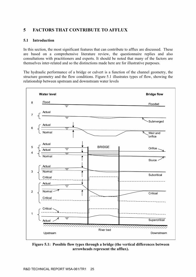
5 FACTORS THAT CONTRIBUTE TO AFFLUX 5.1 Introduction In this section, the most significant features that can contribute to afflux are discussed. These are based on a comprehensive literature review, the questionnaire replies and also consultations with practitioners and experts. It should be noted that many of the factors are themselves inter-related and so the distinctions made here are for illustrative purposes. The hydraulic performance of a bridge or culvert is a function of the channel geometry, the structure geometry and the flow conditions. Figure 5.1 illustrates types of flow, showing the relationship between upstream and downstream water levels
Figure 5.1: Possible flow types through a bridge (the vertical differences between
arrowheads represent the afflux).
R&D TECHNICAL REPORT W5A-061/TR1 26
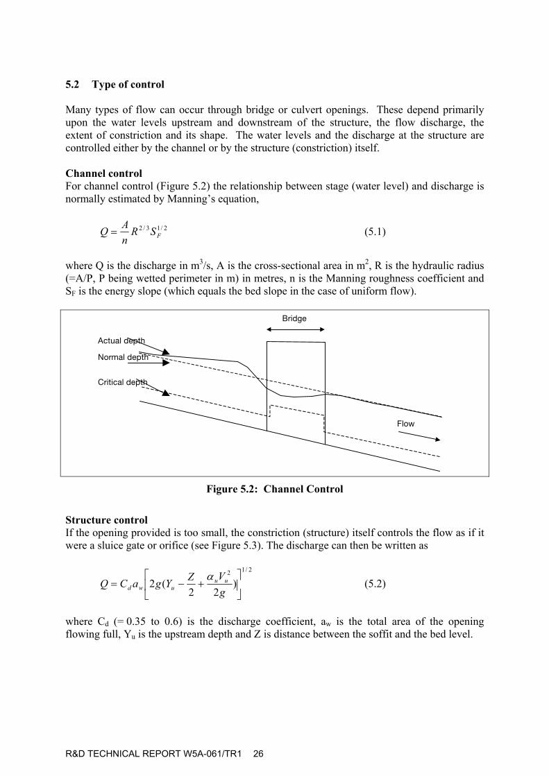
5.2 Type of control Many types of flow can occur through bridge or culvert openings. These depend primarily upon the water levels upstream and downstream of the structure, the flow discharge, the extent of constriction and its shape. The water levels and the discharge at the structure are controlled either by the channel or by the structure (constriction) itself.
Channel control For channel control (Figure 5.2) the relationship between stage (water level) and discharge is normally estimated by Manning’s equation,
2/13/2FSR
nAQ = (5.1)
where Q is the discharge in m3/s, A is the cross-sectional area in m2, R is the hydraulic radius (=A/P, P being wetted perimeter in m) in metres, n is the Manning roughness coefficient and SF is the energy slope (which equals the bed slope in the case of uniform flow).
=================
_êáÇÖÉ
`êáíáÅ~ä=ÇÉéíÜ=
kçêã~ä=ÇÉéíÜ=
^Åíì~ä=ÇÉéíÜ=
cäçï=
Figure 5.2: Channel Control
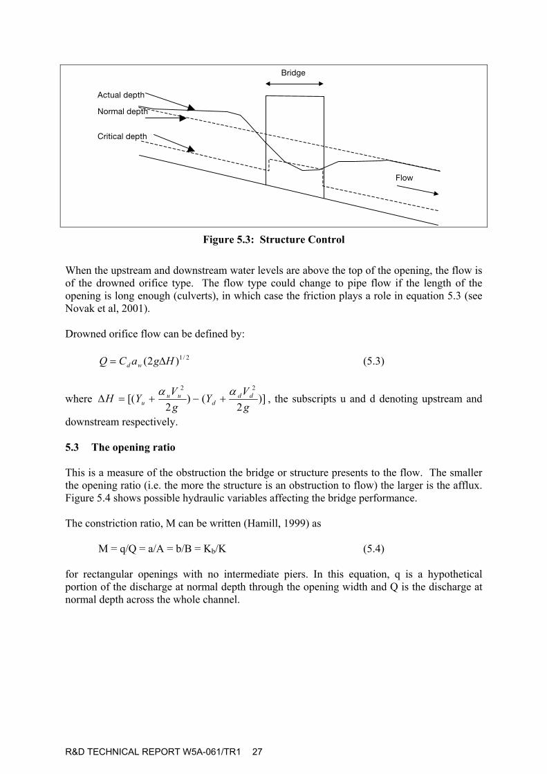
Structure control If the opening provided is too small, the constriction (structure) itself controls the flow as if it were a sluice gate or orifice (see Figure 5.3). The discharge can then be written as
2/12
)22
(2
+−=
gVZYgaCQ uu
uwdα
(5.2)
where Cd (= 0.35 to 0.6) is the discharge coefficient, aw is the total area of the opening flowing full, Yu is the upstream depth and Z is distance between the soffit and the bed level.
R&D TECHNICAL REPORT W5A-061/TR1 27
================
=
_êáÇÖÉ
`êáíáÅ~ä=ÇÉéíÜ=
kçêã~ä=ÇÉéíÜ=
^Åíì~ä=ÇÉéíÜ=
cäçï=
Figure 5.3: Structure Control
When the upstream and downstream water levels are above the top of the opening, the flow is of the drowned orifice type. The flow type could change to pipe flow if the length of the opening is long enough (culverts), in which case the friction plays a role in equation 5.3 (see Novak et al, 2001). Drowned orifice flow can be defined by: 2/1)2( HgaCQ wd ∆= (5.3)
where )]2
()2
[(22
gVY
gVYH dd
duu
uαα
+−+=∆ , the subscripts u and d denoting upstream and
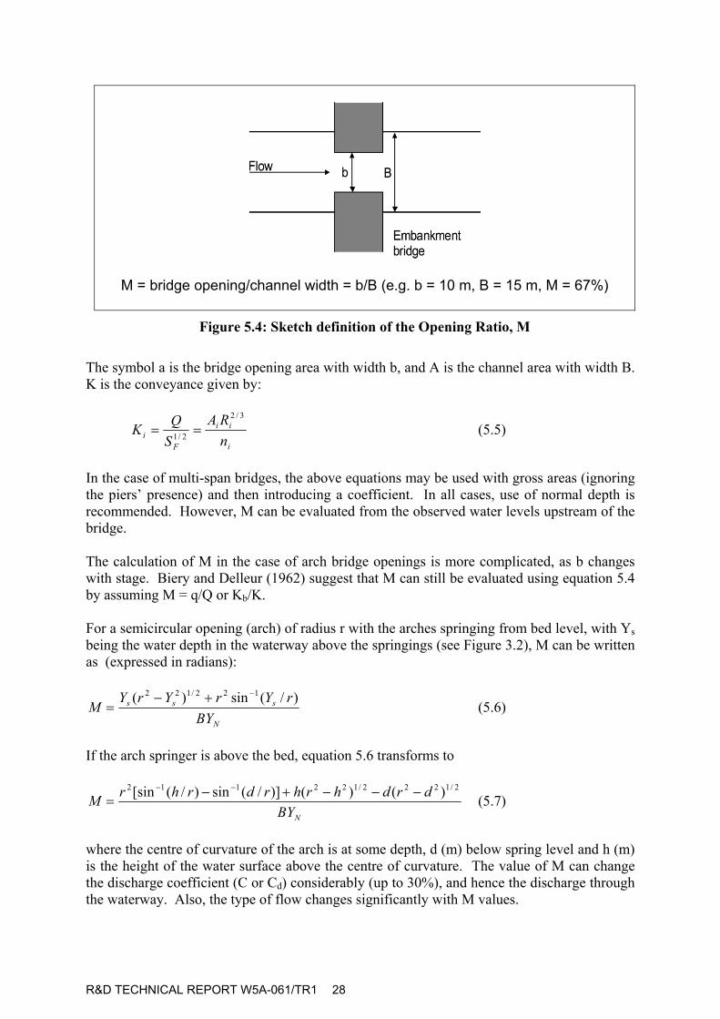
downstream respectively. 5.3 The opening ratio This is a measure of the obstruction the bridge or structure presents to the flow. The smaller the opening ratio (i.e. the more the structure is an obstruction to flow) the larger is the afflux. Figure 5.4 shows possible hydraulic variables affecting the bridge performance. The constriction ratio, M can be written (Hamill, 1999) as M = q/Q = a/A = b/B = Kb/K (5.4) for rectangular openings with no intermediate piers. In this equation, q is a hypothetical portion of the discharge at normal depth through the opening width and Q is the discharge at normal depth across the whole channel.
R&D TECHNICAL REPORT W5A-061/TR1 28
M = bridge opening/channel width = b/B (e.g. b = 10 m, B = 15 m, M = 67%)
Figure 5.4: Sketch definition of the Opening Ratio, M The symbol a is the bridge opening area with width b, and A is the channel area with width B. K is the conveyance given by:
i
ii
Fi n
RASQK
3/2
2/1 == (5.5)
In the case of multi-span bridges, the above equations may be used with gross areas (ignoring the piers’ presence) and then introducing a coefficient. In all cases, use of normal depth is recommended. However, M can be evaluated from the observed water levels upstream of the bridge. The calculation of M in the case of arch bridge openings is more complicated, as b changes with stage. Biery and Delleur (1962) suggest that M can still be evaluated using equation 5.4 by assuming M = q/Q or Kb/K. For a semicircular opening (arch) of radius r with the arches springing from bed level, with Ys being the water depth in the waterway above the springings (see Figure 3.2), M can be written as (expressed in radians):
N
sss
BYrYrYrY
M)/(sin)( 122/122 −+−
= (5.6)
If the arch springer is above the bed, equation 5.6 transforms to
NBYdrdhrhrdrhrM
2/1222/122112 )()()]/(sin)/([sin −−−+−=
−−
(5.7)
where the centre of curvature of the arch is at some depth, d (m) below spring level and h (m) is the height of the water surface above the centre of curvature. The value of M can change the discharge coefficient (C or Cd) considerably (up to 30%), and hence the discharge through the waterway. Also, the type of flow changes significantly with M values.
R&D TECHNICAL REPORT W5A-061/TR1 29
In the cases of single and multiple arch bridges, HR Wallingford (1988) suggests two ‘blockage ratios’ (J1 and J2) which in turn are used to determine the afflux. J1 is defined as the upstream blockage ratio (area of blockage of bridge at depth Y1/area of flow) whereas J2 is the downstream blockage ratio (area of blockage of bridge at depth Y3/area of flow). 5.4 Froude number The Froude number, F, is a measure of the ratio of inertial forces to gravity forces, and is defined by
2/1
3
2
=
gABQF Tα , (5.8)
where BT is the top width of the water surface (m) between the banks. The type of flow is largely determined by the Froude number. The Froude number is unity at the point of control in an open channel where critical depth is formed (see Figure 5.2). In most river channels, the flow is subcritical. Some afflux estimation methods (e.g. the USGS method) use the Froude number at the point of minimum cross sectional flow area, which may be within the bridge waterway; this location corresponds to cross section No. 3 in Figure 3.3, and the Froude number here is denoted F3. With arched openings BT reduces with increase in stage and the solution becomes dubious. Hamill (1993) suggested the use of the bottom width of the arch when calculating F3 and critical depths. As the flow opening contracts, the bridge flow progressively changes to critical. The limiting (critical) contraction is suggested by Yarnell (1934) as
321
21
)2(27
FFM L +
= , (5.9)
where subscripts correspond to the locations of cross sections 1 to 4 shown in Figure 3.3. Henderson (1966) modified this with the assumption that the momentums at sections 3 and 4 are equal, thus
324
44
3
)1()/12(
FFMM L
L ++
= . (5.10)
Flow conditions that can occur through a structure are illustrated further in Section 10 (Figure 10.3).

R&D TECHNICAL REPORT W5A-061/TR1 30
5.5 Choking of bridge opening Flow through a constriction may be dominated by the ‘choking’ phenomenon. Choking is usually associated with critical or supercritical flow at structures with particularly large reductions in waterway width. It occurs where the constriction in flow is more severe than the limiting contraction (as discussed above). The water level increases upstream of the structure to enable the transition from subcritical to supercritical flow. This is manifest in the real world as a rapid rise in the upstream water level for little or no change in discharge. The process of choking can be described in terms of the relationship between depth at a section and the specific energy (which is the energy above bed level, equal to the sum of the depth of flow and velocity head). Figure 5.5 shows three such possible depth/energy relationships for different values of specific discharge (i.e. discharge per unit width). For a given total flow, the effect of making a constriction narrower is to increase the specific discharge through the constriction as shown. For subcritical flow, this can be achieved by an acceleration (driven by an increase in upstream water level). The acceleration is balanced by a decrease in depth which means that there is no change in specific energy required. This situation is illustrated in Figure 5.5 by the transition from point ‘A’ to point ‘B’. Point ‘B’ has been chosen to be at critical depth (i.e. the limiting contraction). For a further contraction, the consequent increase in specific discharge cannot be accomplished at the same specific energy, but requires a shift to the right on the graph, representing an increase in specific energy. This increase in energy leads to an increase in upstream water depth. If choking occurs then the effect is thus to increase upstream water levels, making the afflux larger.
Figure 5.5: Relationship between depth and specific energy showing the effect of choking (after Hamill, 1999)
Most methods of calculating afflux treat the flow as subcritical and do not allow for choking. Choking is not easy to predict and the problem of debris caught on the piers or abutments would always aggravate the situation.
R&D TECHNICAL REPORT W5A-061/TR1 31
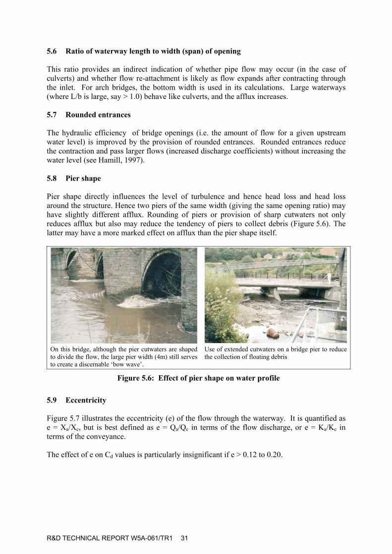
5.6 Ratio of waterway length to width (span) of opening This ratio provides an indirect indication of whether pipe flow may occur (in the case of culverts) and whether flow re-attachment is likely as flow expands after contracting through the inlet. For arch bridges, the bottom width is used in its calculations. Large waterways (where L/b is large, say > 1.0) behave like culverts, and the afflux increases. 5.7 Rounded entrances The hydraulic efficiency of bridge openings (i.e. the amount of flow for a given upstream water level) is improved by the provision of rounded entrances. Rounded entrances reduce the contraction and pass larger flows (increased discharge coefficients) without increasing the water level (see Hamill, 1997). 5.8 Pier shape Pier shape directly influences the level of turbulence and hence head loss and head loss around the structure. Hence two piers of the same width (giving the same opening ratio) may have slightly different afflux. Rounding of piers or provision of sharp cutwaters not only reduces afflux but also may reduce the tendency of piers to collect debris (Figure 5.6). The latter may have a more marked effect on afflux than the pier shape itself.
On this bridge, although the pier cutwaters are shaped to divide the flow, the large pier width (4m) still serves to create a discernable ‘bow wave’.
Use of extended cutwaters on a bridge pier to reduce the collection of floating debris
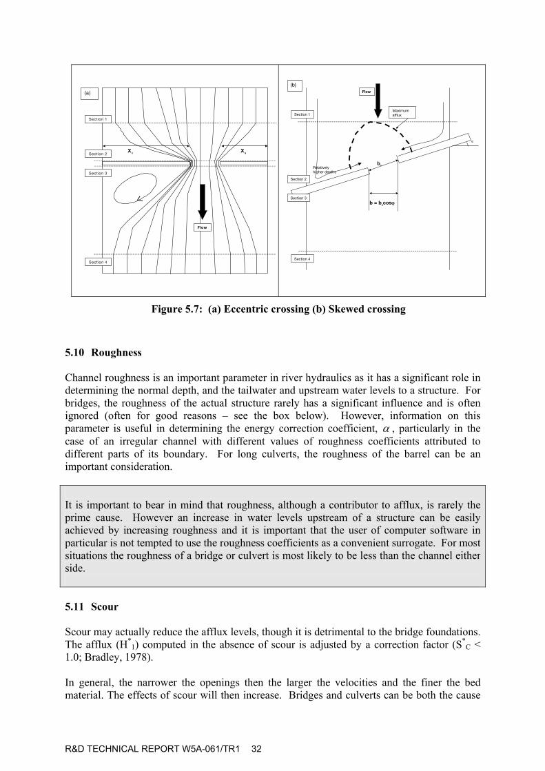
Figure 5.6: Effect of pier shape on water profile 5.9 Eccentricity Figure 5.7 illustrates the eccentricity (e) of the flow through the waterway. It is quantified as e = Xa/Xc, but is best defined as e = Qa/Qc in terms of the flow discharge, or e = Ka/Kc in terms of the conveyance. The effect of e on Cd values is particularly insignificant if e > 0.12 to 0.20.
R&D TECHNICAL REPORT W5A-061/TR1 32
==================================================
=
cäçï=
pÉÅíáçå=N=
pÉÅíáçå=O=
pÉÅíáçå=P=
pÉÅíáçå=Q=
uÅ= u~
E~F=
=================================================
=
cäçï
pÉÅíáçå=N
pÉÅíáçå=O
pÉÅíáçå=Q
j~ñáãìã==~ÑÑäìñ=
pÉÅíáçå=P
ϕ
Äë
Ä=Z=ÄëÅçëϕ=
oÉä~íáîÉäó=ÜáÖÜÉê=ÇÉéíÜë
EÄF
Figure 5.7: (a) Eccentric crossing (b) Skewed crossing 5.10 Roughness Channel roughness is an important parameter in river hydraulics as it has a significant role in determining the normal depth, and the tailwater and upstream water levels to a structure. For bridges, the roughness of the actual structure rarely has a significant influence and is often ignored (often for good reasons – see the box below). However, information on this parameter is useful in determining the energy correction coefficient, α , particularly in the case of an irregular channel with different values of roughness coefficients attributed to different parts of its boundary. For long culverts, the roughness of the barrel can be an important consideration. It is important to bear in mind that roughness, although a contributor to afflux, is rarely the prime cause. However an increase in water levels upstream of a structure can be easily achieved by increasing roughness and it is important that the user of computer software in particular is not tempted to use the roughness coefficients as a convenient surrogate. For most situations the roughness of a bridge or culvert is most likely to be less than the channel either side. 5.11 Scour Scour may actually reduce the afflux levels, though it is detrimental to the bridge foundations. The afflux (H*
1) computed in the absence of scour is adjusted by a correction factor (S*C <
1.0; Bradley, 1978). In general, the narrower the openings then the larger the velocities and the finer the bed material. The effects of scour will then increase. Bridges and culverts can be both the cause
R&D TECHNICAL REPORT W5A-061/TR1 33
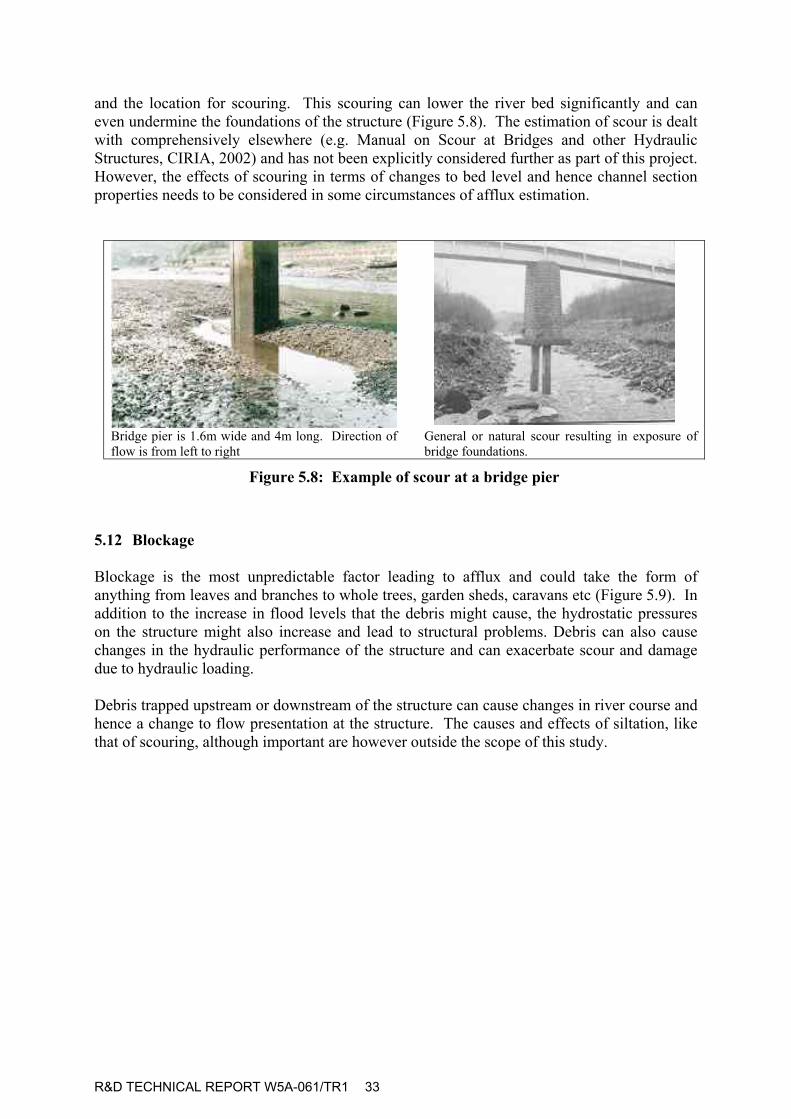
and the location for scouring. This scouring can lower the river bed significantly and can even undermine the foundations of the structure (Figure 5.8). The estimation of scour is dealt with comprehensively elsewhere (e.g. Manual on Scour at Bridges and other Hydraulic Structures, CIRIA, 2002) and has not been explicitly considered further as part of this project. However, the effects of scouring in terms of changes to bed level and hence channel section properties needs to be considered in some circumstances of afflux estimation.
Bridge pier is 1.6m wide and 4m long. Direction of flow is from left to right
General or natural scour resulting in exposure of bridge foundations.
Figure 5.8: Example of scour at a bridge pier
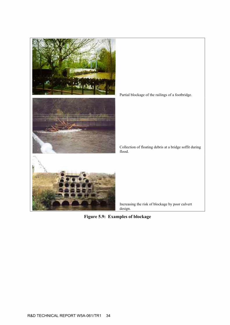
5.12 Blockage Blockage is the most unpredictable factor leading to afflux and could take the form of anything from leaves and branches to whole trees, garden sheds, caravans etc (Figure 5.9). In addition to the increase in flood levels that the debris might cause, the hydrostatic pressures on the structure might also increase and lead to structural problems. Debris can also cause changes in the hydraulic performance of the structure and can exacerbate scour and damage due to hydraulic loading. Debris trapped upstream or downstream of the structure can cause changes in river course and hence a change to flow presentation at the structure. The causes and effects of siltation, like that of scouring, although important are however outside the scope of this study.
R&D TECHNICAL REPORT W5A-061/TR1 34
Partial blockage of the railings of a footbridge.
Collection of floating debris at a bridge soffit during flood.
Increasing the risk of blockage by poor culvert design.
Figure 5.9: Examples of blockage

R&D TECHNICAL REPORT W5A-061/TR1 35
Table 5.1: Variables that affect afflux
Variable
Likely effect on upstream water levels/afflux
Opening Ratio (M) The smaller the opening ratio, the larger the afflux. If very high, may cause choking of the inlet.
Froude Number (F) Generally the higher the Froude Number, the larger the afflux. (This is the Froude Number for flow in the channel, in the absence of the structure).
Choking of bridge opening
Afflux increases when flow is choked.
Length/breadth Ratio (L/b)
If ratio is high (L/b > 1.0) then afflux generally increases
Rounding of the entrance/ Rounding of Piers
The smoother the entry, the less turbulence and hence the lower the afflux. Smoothing/rounding can also help to reduce blockage risk.
Eccentricity, e For e < 0.2, afflux is generally reduced.
Skew The larger the skew of a structure relative to the direction of flow, the larger the afflux. For skew angles of less than 20o, the effect is usually negligible.
Roughness The larger the roughness, the larger the afflux.
Scour Generally reduces bed levels and hence decreases afflux.
Blockage Decreases the opening ratio and increases turbulence at the entrance. Nearly always results in a higher water level.

R&D TECHNICAL REPORT W5A-061/TR1 36
R&D TECHNICAL REPORT W5A-061/TR1 37
6 METHODS OF ESTIMATING AFFLUX 6.1 Introduction This chapter begins by describing the principle theoretical approaches to afflux calculation. The chapter then gives an overview of the main methods for calculating afflux for various types of bridge and culvert structures under different hydraulic conditions. The principles of afflux calculation are discussed here, whilst details of the specific methods are given in Appendix A. The discussion draws on an expert paper by Knight (2001), commissioned for this study to review current knowledge on bridge afflux, and attached as Annex 1 to this report. A similar paper by Samuels (2001), attached as Annex 2, reviews the implementation of afflux estimation in hydraulic models. 6.2 Theoretical approaches to afflux calculation There are two main representations used for estimating the afflux upstream of a bridge. The first representation assumes that the afflux (∆Y) is a proportion of the kinetic energy of the flow through a bridge, thus:
∆Y = K*V2/2g (6.1)
where K is a friction factor, V is the mean velocity through the bridge, and g the acceleration of gravity. The second representation uses the afflux as an independent variable in representing the flow discharge (Q), thus:
Q = CA* f(∆Y) (6.2)
where C is a dimensional discharge coefficient, A is the area of flow through the bridge, and f(∆Y) is a function of the afflux. These methods apply to the pier bridges and embankment bridges, as described below. The basis for the representations is estimation of the energy loss caused by the structure, which leads to the increased upstream level or afflux that is required for a steady flow. The rationale for the two representations of afflux is best illustrated by considering their application to steady, uniform flow in a river channel. In river hydraulics, the dimensionless relationships for steady open channel flow can be adapted from pipe flow equations (Roberson et al, 1997). For example, the head loss (hf) for turbulent flow in pipes is given by the Darcy-Weisbach formula as:
hf = f *L/D*V2/2g (6.3) where f is a pipe friction factor (which may be interpolated from a Moody diagram), L is the pipe length, D the pipe diameter, V the mean velocity of flow in the pipe and g the gravitational acceleration. This formula is adapted to channels by noting that the head loss in an open channel is given by (S * L) where S is the channel slope and L the channel length. The pipe diameter (D) is replaced by 4R for a channel, where R is called the “hydraulic”
R&D TECHNICAL REPORT W5A-061/TR1 38
radius denoted by the area/perimeter ratio. By equating the head losses, the channel velocity and flow are is solved as
V = (8g/f)0.5 * (RS)0.5 (6.4) and Q = (8g/f)0.5A * (RS)0.5 (6.5) where A is the area of the channel. Thus (8g/f)0.5 is the discharge coefficient (C) for uniform flow, and the two representations are equivalent. For bridge hydraulics, however, the friction factor and discharge coefficient depend upon many more variables (as discussed in Section 5), owing to the heterogeneity of the bridge structural geometry and incident flows. A unique solution, as for the case of steady flow river hydraulics, has therefore not yet been achieved. 6.2.1 Theoretical approaches – An example of the friction factor representation for a
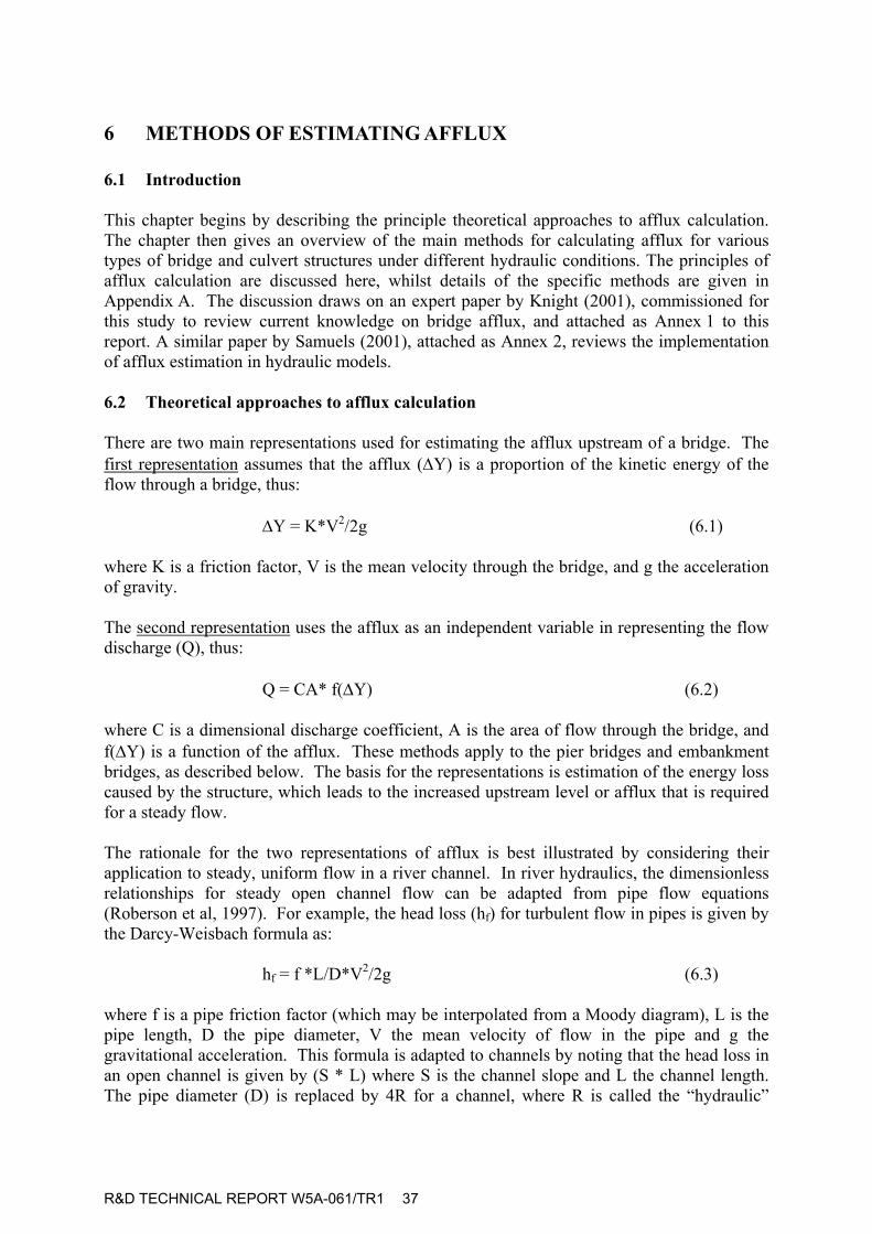
pier bridge A “pier bridge” is defined herein as crossing the entire flood plain, being supported by several piers, and usually located in a rural setting. The resistance to flow is caused mainly by the presence of the piers (Figure 6.1(a) illustrates a simplified type). The laws for the conservation of mass and momentum have been applied to a simplified pier bridge (Montes, 1998), and it was shown that the result approximates the friction factor method.
Bridge deck
Bridge deck
Embankment soffit
Floodplain
Floodplain
Main channel
Pier
Main channel
(a)
(b)
Abutment
Figure 6.1: (a) Pier bridge (b) Embankment bridge
R&D TECHNICAL REPORT W5A-061/TR1 39
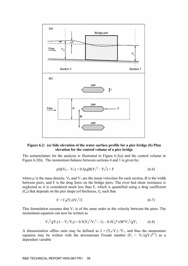
Figure 6.2: (a) Side elevation of the water surface profile for a pier bridge (b) Plan elevation for the control volume of a pier bridge
The nomenclature for the analysis is illustrated in Figure 6.2(a) and the control volume in Figure 6.2(b). The momentum balance between sections 4 and 1 is given by:
ρQ(V4 – V1) = 0.5ρgB(Y12 – Y4
2) + F (6.6) where ρ is the mass density, V4 and V1 are the mean velocities for each section, B is the width between piers, and F is the drag force on the bridge piers. The river bed shear resistance is neglected as it is considered much less than F, which is quantified using a drag coefficient (Cd) that depends on the pier shape (of thickness, t), such that
F = Cd(Y1t)V12/2 (6.7)
This formulation assumes that V1 is of the same order as the velocity between the piers. The momentum equation can now be written as
V12/gY1(1 – Y1/Y4) = 0.5(Y4
2/Y12 – 1) – 0.5Cd* t/B*V1
2/gY1 (6.8) A dimensionless afflux ratio may be defined as λ = (Y4-Y1) /Y1, and thus the momentum equation may be written with the downstream Froude number (F1 = V1/(gY1)0.5) as a dependent variable
R&D TECHNICAL REPORT W5A-061/TR1 40
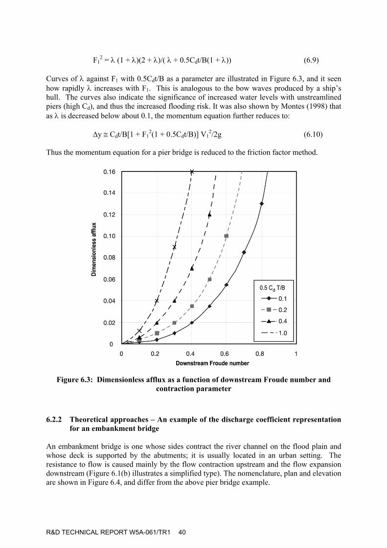
F1
2 = λ (1 + λ)(2 + λ)/( λ + 0.5Cdt/B(1 + λ)) (6.9) Curves of λ against F1 with 0.5Cdt/B as a parameter are illustrated in Figure 6.3, and it seen how rapidly λ increases with F1. This is analogous to the bow waves produced by a ship’s hull. The curves also indicate the significance of increased water levels with unstreamlined piers (high Cd), and thus the increased flooding risk. It was also shown by Montes (1998) that as λ is decreased below about 0.1, the momentum equation further reduces to:
∆y ≅ Cdt/B[1 + F12(1 + 0.5Cdt/B)] V1
2/2g (6.10) Thus the momentum equation for a pier bridge is reduced to the friction factor method.
Figure 6.3: Dimensionless afflux as a function of downstream Froude number and contraction parameter
6.2.2 Theoretical approaches – An example of the discharge coefficient representation
for an embankment bridge An embankment bridge is one whose sides contract the river channel on the flood plain and whose deck is supported by the abutments; it is usually located in an urban setting. The resistance to flow is caused mainly by the flow contraction upstream and the flow expansion downstream (Figure 6.1(b) illustrates a simplified type). The nomenclature, plan and elevation are shown in Figure 6.4, and differ from the above pier bridge example.
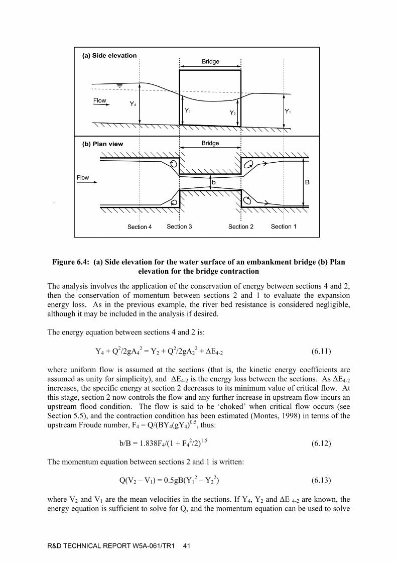
R&D TECHNICAL REPORT W5A-061/TR1 41
Figure 6.4: (a) Side elevation for the water surface of an embankment bridge (b) Plan elevation for the bridge contraction
The analysis involves the application of the conservation of energy between sections 4 and 2, then the conservation of momentum between sections 2 and 1 to evaluate the expansion energy loss. As in the previous example, the river bed resistance is considered negligible, although it may be included in the analysis if desired. The energy equation between sections 4 and 2 is:
Y4 + Q2/2gA42 = Y2 + Q2/2gA2
2 + ∆E4-2 (6.11) where uniform flow is assumed at the sections (that is, the kinetic energy coefficients are assumed as unity for simplicity), and ∆E4-2 is the energy loss between the sections. As ∆E4-2 increases, the specific energy at section 2 decreases to its minimum value of critical flow. At this stage, section 2 now controls the flow and any further increase in upstream flow incurs an upstream flood condition. The flow is said to be ‘choked’ when critical flow occurs (see Section 5.5), and the contraction condition has been estimated (Montes, 1998) in terms of the upstream Froude number, F4 = Q/(BY4(gY4)0.5, thus:
b/B = 1.838F4/(1 + F42/2)1.5 (6.12)
The momentum equation between sections 2 and 1 is written:
Q(V2 – V1) = 0.5gB(Y12 – Y2
2) (6.13)
where V2 and V1 are the mean velocities in the sections. If Y4, Y2 and ∆E 4-2 are known, the energy equation is sufficient to solve for Q, and the momentum equation can be used to solve
R&D TECHNICAL REPORT W5A-061/TR1 42
for Y1 and thus the afflux (Y4 – Y1). Unfortunately, it is Y1 that is usually known from a normal flow or backwater condition, and the solution for Y2 then becomes an iterative problem. Furthermore, the energy loss ∆E4-2 is a complex function of the bridge geometry and flow. It can however be analysed using the discharge coefficient method as follows. The energy loss between sections 4 and 2 is due to frictional and eddy losses in the contraction, and is written in terms of a loss coefficient,
∆E4-2 = K4-2* Q2/2g(bY2)2 (6.14)
Substituting this term into the energy equation, an implicit equation for Q may be written using the discharge coefficient representation, thus:
Q = CbY2 * [2g(Y4-Y2 + Q2/2gA42 – K 4-2* Q2/2g(bY2)2]0.5 (6.15)
The discharge coefficient C has been evaluated for many contraction geometries and flow types by Kindsvater and Carter (1953), and is described more fully below. Note however that unless the momentum equation from section 3 to 4 is solved, then the true afflux (Y4-Y1) cannot be computed. The preceding paragraphs in Section 6.2 have discussed theoretical principles applied to calculate afflux. Specific methods for afflux calculation, for different structures and flow conditions, are considered below in Sections 6.3 to 6.8. 6.3 Afflux calculation methods for pier bridges Some of the early researches into bridge hydraulics were mainly concerned with pier bridges. The work of d’Aubuisson (1840) and Nagler (1917) are examples of the discharge coefficient representation, and the work of Rehbock (1921) and Yarnell (1934) are examples of the friction factor representation. They are summarised below. 6.3.1 Discharge coefficient representation (pier bridges) Following from the previous discharge coefficient representation (Equation 6.15), d’Aubuisson assumed that Y2 = Y1, and the energy loss ∆E4-2 was negligible, thus:
Q = CAbY1 * [2g(Y4-Y1 + V42/2g)]0.5 (6.16)
Nagler (1917) expanded this relation by introducing the energy loss as a coefficient (η) for the upstream velocity head. He also assumed that C was directly influenced by the downstream Froude number, F1 = V1/(gY1)0.5, thus:
Q = CNbY1 * (1- θF12)[2g(Y4-Y1 + ηV4
2/2g)]0.5 (6.17)
The coefficients θ and η are coefficients to account for the contraction ratio (b/B) and energy losses between sections 4 and 2. An approximate value of θ = 0.15 was given by Nagler, and η was estimated as:
η = 1 + 1.05tanh[4.5(1 – b/B)] (6.18)
R&D TECHNICAL REPORT W5A-061/TR1 43
The discharge coefficients CA and CN for the above representations were determined empirically, and depended principally on the pier shape. The most reliable values are those determined by Yarnell (1933) from a series of 2600 laboratory measurements. 6.3.2 Friction factor representation (pier bridges) Both Rehbock (1921) and Yarnell (1934) used the friction factor representation for pier bridges, and assumed a functional relation for K as:
K = K( α, F1, δ ) (6.19) where α = 1-b/B and is a measure of the contraction, F1 is the downstream Froude number, and δ is a pier shape coefficient. The functional forms of these coefficients were determined empirically as:
Rehbock: KR = (δ – α(δ – 1))(0.4α + α2 + 9α4)(1 + F12) (6.20)
Yarnell: KY = 2δ(δ + 5F1
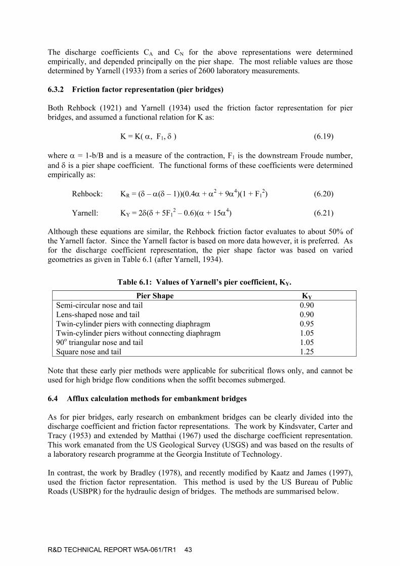
2 – 0.6)(α + 15α4) (6.21) Although these equations are similar, the Rehbock friction factor evaluates to about 50% of the Yarnell factor. Since the Yarnell factor is based on more data however, it is preferred. As for the discharge coefficient representation, the pier shape factor was based on varied geometries as given in Table 6.1 (after Yarnell, 1934).
Table 6.1: Values of Yarnell’s pier coefficient, KY.
Pier Shape KY Semi-circular nose and tail 0.90 Lens-shaped nose and tail 0.90 Twin-cylinder piers with connecting diaphragm 0.95 Twin-cylinder piers without connecting diaphragm 1.05 90o triangular nose and tail 1.05 Square nose and tail 1.25
Note that these early pier methods were applicable for subcritical flows only, and cannot be used for high bridge flow conditions when the soffit becomes submerged. 6.4 Afflux calculation methods for embankment bridges As for pier bridges, early research on embankment bridges can be clearly divided into the discharge coefficient and friction factor representations. The work by Kindsvater, Carter and Tracy (1953) and extended by Matthai (1967) used the discharge coefficient representation. This work emanated from the US Geological Survey (USGS) and was based on the results of a laboratory research programme at the Georgia Institute of Technology. In contrast, the work by Bradley (1978), and recently modified by Kaatz and James (1997), used the friction factor representation. This method is used by the US Bureau of Public Roads (USBPR) for the hydraulic design of bridges. The methods are summarised below.
R&D TECHNICAL REPORT W5A-061/TR1 44
6.4.1 Discharge coefficient representation (embankment bridges)
The Kindsvater and Carter method attempted to evaluate the discharge coefficient (C) for a universal range of bridge openings. The results were based on an extensive laboratory study and its verification using 30 field sites. The discharge coefficient was derived as summarised in 6.3, thus:
Q = CbY2 * [2g(Y4-Y2 + Q2/2gA42 – K4-2* Q2/2g(bY2)2]0.5 (6.22)
The procedure has been documented fully in hydraulics textbooks (Chow, 1981; French, 1986; Hamill, 1999) and only the main principles are given herein. In general, bridge openings were classified into four types, as follows:
1. Vertical embankments and vertical abutments, with or without wingwalls. 2. Sloping embankments and vertical abutments. 3. Sloping embankments and sloping abutments. 4. Sloping embankments and vertical abutments with wingwalls.
For each type, the discharge coefficient was determined as a function of the bridge geometry and flow. For example
C = C(b/B, L/b, r/b,ϕ, e, F2) (6.23) where L is the length of the bridge contraction, r is the radius of curvature at the contraction entry, ϕ is the skew or angle that the axis of contraction differs from the flow direction, and e is the eccentricity or distance off-centre of the bridge opening from the axis of symmetry of the channel flow. When these design coefficients were evaluated for a field measurement, Kindsvater and Carter found that the field results differed by less than 5%. The method was also extended with further coefficients to multiple openings, spur dykes (guide walls at the bridge approach), and submerged bridges. Note again that the method does not give afflux directly from the discharge calculation. The momentum equation or energy loss from section 2 to 1 is required to compute the downstream elevation for estimating afflux. As an alternative, Kindsvater and Carter (1955) gave an empirical method for estimating the afflux that used two design charts. 6.4.2 Friction factor representation (embankment bridges) The Bradley method for estimating afflux begins by considering the energy equation between sections 4 and 1 (Figure 6.4), which can be written
Y4 + Q2/2gA42 = Y1 + Q2/2gA1
2 + ∆E4-1 . (6.24)
The friction factor representation is then used to estimate the energy loss,
∆E4-1 = K * (α3VN32/2g) , (6.25)
where α3 is the velocity distribution coefficient for non-uniform flow, and VN3 is a reference velocity equal to Q/AN3. The area AN3 is the hypothetical area in the contraction subtended by
R&D TECHNICAL REPORT W5A-061/TR1 45
the normal depth of the channel in the absence of the contraction. Thus VN3 can be readily calculated for a bridge obstruction in a flow at normal depth. Substituting the friction factor representation in the energy equation gives the afflux as:
∆y = K * (α3VN32/2g) + α3V3
2/2g – α4V42/2g (6.26)
If it is assumed that the velocity distributions at sections 4 and 1 are similar, then α4 = α1. By conservation of mass, A1V1 = A4V4 = AN3VN3, thus the above equation may be simplified to:
∆y = K * (α3VN32/2g) + α4[(AN3/A1)2 – (AN3/A4 )2]VN3
2/2g (6.27) The flow variability is now governed by the velocity distribution coefficients, as opposed to the downstream Froude number as used in the discharge coefficient method. Ideally, α1
should be estimated from a velocity traverse, and a design chart can be used to estimate α3 as a function of b/B. Thus given K and α4, the afflux equation may be solved iteratively. The friction factor K is calculated as a function of the bridge geometry using incremental coefficients, thus:
K = Kb + Ke + Kϕ + Kp (6.28) where Kb is the main coefficient depending on the contraction ratio (b/B) and the geometry of the abutments (similar to the bridge opening types in the Kindsvater and Carter method). The other coefficients represent the influence of eccentricity, skew and the type and number of bridge piers. In addition to estimating afflux for subcritical flows, Bradley (1978) has extended the method to the following situations:
1. Difference in water level across approach embankments. 2. Dual bridges. 3. Abnormal stage-discharge conditions. 4. Effect of scour on backwater. 5. Superstructure partially inundated. 6. Spur dykes. 7. Flow passing through critical depth.
Note that the method is more direct than the Kindsvater and Carter method, but it requires a knowledge of the velocity distribution for estimating the α1 coefficient. 6.5 Afflux calculation for arched bridges There are two major studies concerned with the hydraulics of arched bridges. These are the work by Biery and Delleur (1962) and the Hydraulics Research study (HR, 1988). In general, both methods conclude with a simple, empirical, functional representation for afflux in the form:
∆Y/YN = f(b/B, FN) (6.29)

R&D TECHNICAL REPORT W5A-061/TR1 46
where the subscript N refers to the downstream section at normal flow. Thus the afflux is simply considered a dimensionless function of the bridge opening ratio and the downstream flow condition (given by the Froude number). The methods are therefore limited to normal, non-eccentric openings. A brief summary of each work follows. 6.5.1 Biery and Delleur method (1962) This appears to be the first laboratory study on single span arch bridges. In addition to presenting equations for the afflux determination (as shown graphically in Hamill, 1999), the following factors were evaluated:
1. Variation of the distance from the bridge face to the section of the afflux with FN and b/B.
2. Variation of the distance between the sections of maximum and minimum water levels with b/B.
3. Variation of the coefficient of discharge for a semi-circular arch with FN and b/B. 6.5.2 HR method (1988) The Hydraulics Research (HR) investigations extended the study of arched bridges to both field and laboratory investigations and to single and multiple arched bridges. The types of bridges analysed were:
1. Model single semicircular arches 2. Model single elliptical arches 3. Model multiple semicircular arches 4. Model multiple semicircular arches with different soffit levels 5. Prototype single arches 6. Prototype multiple arches
Instead of an opening ratio, HR defined a blockage ratio defined as the ratio between the structural blockage to flow and the total flow area. This ratio varies through the bridge due to the differing water depths and flow areas. As a consequence, three design charts were produced:
1. Variation of afflux with downstream Froude number and downstream blockage ratio for all bridges.
2. Variation of afflux with downstream Froude number and upstream blockage ratio for single arches.
3. Variation of afflux with downstream Froude number and upstream blockage ratio for multiple arches.
6.6 Modern computational applications of afflux calculation methods The major problem with the above methods is that they all attempt to represent the energy losses in all three bridge ‘reaches’ shown in Figure 6.4, (i.e. section 1 to section 2 (the contraction), section 2 to section 3 (bridge waterway) and section 3 to section 4 (expansion)) with a single empirical coefficient. They therefore provide an order of magnitude estimate for afflux using hand calculation. With computer modelling, it is possible to solve complex water

R&D TECHNICAL REPORT W5A-061/TR1 47
level problems iteratively by dividing a river into reaches and solving from the upstream or downstream control (or boundary condition). This same method can be used for the three bridge reaches, and thus a more accurate solution may be attained by estimating energy loss coefficients for each reach. Three examples are chosen to summarise these methods, namely the Schneider et al method (USGS, 1977) used in the WSPRO program (FHWA, 1986), and the energy and momentum methods used in the HEC-RAS program (USACE, 1995). 6.6.1 Schneider et al. (1977) method in WSPRO The energy losses for each reach are represented in terms of the conveyance (Ki), where the subscript i refers to the reach identification. The conveyance is defined by Q = KiS0.5 , and thus the energy head loss for a reach is given by
∆Ei = Li * Si = Q2Li/KI . (6.30) For the approach (contraction) reach, then friction losses are
∆E4-3 = Q2L4-3/K4Kc , (6.31) where L4-3 is tabulated, and Kc is the smaller of conveyances between K2 and Kq (Kq is the portion of section 4 conveyance contained within the bridge). For the constricted (bridge) section:
∆E3-2= Q2L3-2/K2 2 (6.32)
For the expansion section, friction losses are:
∆E2-1 = Q2L2-1/K1Kc (6.33) And also for the expansion section, turbulent losses are given by:
∆E2-1 = Q2 /2gA1 2 [2( β1 – α1) – 2β2(A1/A2) + α2(A1/A2)2] (6.34)
where β is the momentum correction coefficient for a section. 6.6.2 Energy method in HEC-RAS (1995) The energy method uses both the conservation of mass and energy for each bridge reach, thus: Mass: Qu = Qd = VuAu = Vd Ad (6.35) Energy: Yu + αuVu
2/2g = Yd + αdVd2/2g + ∆E u-d (6.36)
where : ∆E u-d = LS + C (αuVu
2/2g - αdVd2/2g) (6.37)
R&D TECHNICAL REPORT W5A-061/TR1 48
The subscripts u and d refer to the upstream and downstream sections for each reach. Note that S is taken as the average friction slope for the reach. This equation can be solved iteratively for each reach, provided that values are entered for the α and C coefficients. 6.6.3 Momentum method in HEC-RAS (1995) The conservation of mss equation is again used, but now combined with the conservation of momentum, such that: Momentum: βu Q2/gAu + Y/
u = βuQ2/gAd + Y/dAd + Fext/ρg + Fw/ρg + Fa/ρg (6.38)
where Y/ is the depth from the water surface to the centre of gravity of the flow section, Fext is the sum of streamwise drag forces such as bed and pier friction, Fw is the streamwise, fluid weight force component, and Fa is the streamwise force component due to different flow sections. Note that since most observations of bridge flow profiles only include water level, then the energy equation is the most frequently used. A recent study by Brunner and Hunt (1995) has documented the evaluation of C coefficients in detail. 6.7 Extreme (high) flow methods Extreme high flows are defined as those that submerge the bridge soffit. These may be further defined in order of increasing height as sluice flows, orifice flows, weir plus orifice flows, and totally submerged flows. The latter condition is a total flood condition for which a new flood plain geometry may well apply. The intermediate high flows use a discharge coefficient equation, since the hydraulics of sluices, orifices and weirs have been previously established. It is therefore inevitable that solutions from each of the computer packages (HEC-RAS, ISIS and MIKE 11) should give similar results. The methods used by HEC-RAS only are therefore summarised below (Brunner and Hunt, 1995). 6.7.1 Sluice flow When water reaches the soffit level, a sluice gate type flow is initiated, and the discharge equation is given by:
Q = CdABU[2g(y3 - z/2 + α3V32/2g)]0.5 (6.39)
where Cd is the discharge coefficient, ABU is the area of the bridge opening at section 3, and z is the vertical distance from the soffit to the river bed inside the bridge reach. 6.7.2 Orifice flow When both the upstream and downstream side of the bridge are submerged, the standard orifice equation is used:
Q = CA(2gH)0.5 (6.40) where H is the difference between upstream and downstream head. The discharge coefficient has a typical value of about 0.8.
R&D TECHNICAL REPORT W5A-061/TR1 49
6.7.3 Weir flow Flow over the bridge and the roadway approaching the bridge is calculated using the standard weir equation:
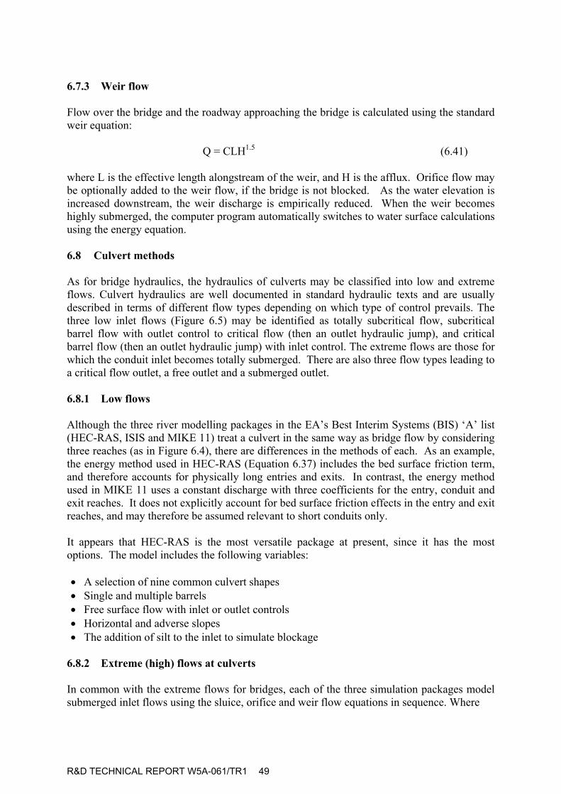
Q = CLH1.5 (6.41) where L is the effective length alongstream of the weir, and H is the afflux. Orifice flow may be optionally added to the weir flow, if the bridge is not blocked. As the water elevation is increased downstream, the weir discharge is empirically reduced. When the weir becomes highly submerged, the computer program automatically switches to water surface calculations using the energy equation. 6.8 Culvert methods As for bridge hydraulics, the hydraulics of culverts may be classified into low and extreme flows. Culvert hydraulics are well documented in standard hydraulic texts and are usually described in terms of different flow types depending on which type of control prevails. The three low inlet flows (Figure 6.5) may be identified as totally subcritical flow, subcritical barrel flow with outlet control to critical flow (then an outlet hydraulic jump), and critical barrel flow (then an outlet hydraulic jump) with inlet control. The extreme flows are those for which the conduit inlet becomes totally submerged. There are also three flow types leading to a critical flow outlet, a free outlet and a submerged outlet. 6.8.1 Low flows Although the three river modelling packages in the EA’s Best Interim Systems (BIS) ‘A’ list (HEC-RAS, ISIS and MIKE 11) treat a culvert in the same way as bridge flow by considering three reaches (as in Figure 6.4), there are differences in the methods of each. As an example, the energy method used in HEC-RAS (Equation 6.37) includes the bed surface friction term, and therefore accounts for physically long entries and exits. In contrast, the energy method used in MIKE 11 uses a constant discharge with three coefficients for the entry, conduit and exit reaches. It does not explicitly account for bed surface friction effects in the entry and exit reaches, and may therefore be assumed relevant to short conduits only. It appears that HEC-RAS is the most versatile package at present, since it has the most options. The model includes the following variables: • A selection of nine common culvert shapes • Single and multiple barrels • Free surface flow with inlet or outlet controls • Horizontal and adverse slopes • The addition of silt to the inlet to simulate blockage
6.8.2 Extreme (high) flows at culverts In common with the extreme flows for bridges, each of the three simulation packages model submerged inlet flows using the sluice, orifice and weir flow equations in sequence. Where
R&D TECHNICAL REPORT W5A-061/TR1 50
Figure 6.5: Unsubmerged and submerged inlet flows through a culvert
necessary, the models can also include road overflow around a structure, and this is integrated in HEC-RAS. 6.9 Measurement of afflux in the field Reliable field data on afflux is very difficult to obtain, partly because it cannot be measured directly and partly because of the logistics of recording flow and levels at bridges and culverts at extreme flows. Ideally, the whole water surface profile is required from the start to the end of backwater water surface. The water surface profile (in the absence of the structure) can be estimated by backwater analysis and subtracted from the measured profile to determine the afflux. If data is measured only at a point then the position depends on the method of analysis. For example, the Kindsvater et al (1953) method requires water levels at sections 4 and 2 (Figure 6.4) whereas the Bradley at al (USBPR, 1978) method requires measurements at sections 4 and 1 (Figure 6.4).
R&D TECHNICAL REPORT W5A-061/TR1 51
With reference again to Figure 6.4, the position of section 4 is sufficiently far upstream of the structure and is normally located at one span (b) upstream of the structure face. The downstream section 2 is parallel to the contraction defining the minimum water depth, and in general is difficult to measure in the field. Section 1 is rather dependent on the nature of the flow expansion downstream of the structure. HEC-RAS suggests a rate of expansion of 1:4 (i.e. it should be at least 2(B-b) from the downstream face of the bridge). Later studies (HEC Report RD-42, 1995) suggest reduced expansion ratios, giving the location of section 1 at around 2b from the downstream face of the bridge. In all cases, the variation of water levels across a section is usually ignored (which is not truly correct). See the report by Kirby and Guganeshrajah (2001) for further information. 6.10 Some examples of field measurements for afflux Hamill (1997) quotes measurements (taken around 1736) at London Bridge indicating a fall (difference in water levels across the bridge) amounting to 1.45 m with an opening ratio, M < 0.5 (Table 6.2). Hamill (1993) also measured afflux at a single arched bridge at Canns Mill in Devon and recorded values as high as 17mm for open channel control, 115mm for structure control and 270mm with the bridge acting as an orifice. Bradley (1978) lists the head loss measurements underpinning his research, the smallest being around 50mm, in a range of 50-900mm. The following field data sets on bridge afflux have been located as part of this review:
• Work by Kaatz and James (1997) • Work by Hamill and McInally (1990) • Work to develop the USGS method (Matthai, 1967) • Work to develop the USBPR method (Bradley, 1978) • Work undertaken to develop HR method for arch bridges (selected bridge sites,
Brown, 1989) • Work related to PhD studies at the University of Birmingham (Atabay and Knight,
2001). The experiments included different floodplain roughness conditions and different types of bridge opening, namely single opening semi-circular arch bridge, multiple opening semi-circular arch bridge, single opening elliptical arch bridge, single opening straight-deck bridge with and without piers including span widths.
Appendix 3 provides further details of these datasets. The quality and usefulness of this data is to be reviewed in Stage 2 of the project. Note that no datasets have been located dealing with culvert blockage. Another potential source of data on afflux could be from past commercial physical model studies. This should in particular provide information on the more unusual structures such as those that are skewed. While much of this data is proprietary, it would be worth investigating further.

R&D TECHNICAL REPORT W5A-061/TR1 52
Table 6.2: Examples of measured bridge afflux/head loss
Location/ Photograph Opening Ratio Afflux/Head loss
Old London Bridge (C12th)
0.31–0.49 The range is due to the reference stage and the existence of ‘starlings’ or skirting around the piers as a form of scour protection.
Fall (head loss) measured as 1.45m in 1736 (Hamill 1999) The difference was used to drive a water wheel
Westminster Bridge, London 0.82 Measured by Labelye as 0.13m (130mm)
Kildwick Bridge, Yorkshire
0.52 – 0.68
Head loss measured by Yorkshire Rivers Authority as 0.5 – 0.6m in flood
6.11 Summary The organisation of afflux methods described in this chapter may be summarised by author or method in Table 6.3.
Table 6.3: Methods for estimating afflux
Class Methods Pier bridges D’Aubuisson
(1840) Nagler (1917)
Yarnell (1934)
Embankment bridges
Kindsvater et al (1953)
Bradley (1978)
Arched bridges Biery and Delleur (1962)
HR, Wallingford (1988)
Computational methods
Schneider et al (1977)
HEC-RAS energy (1995)
HEC-RAS momentum (1995)
High flow Methods
Sluice gate flow Orifice flow Weir flow
Culvert methods HEC-RAS ISIS MIKE 11
R&D TECHNICAL REPORT W5A-061/TR1 53
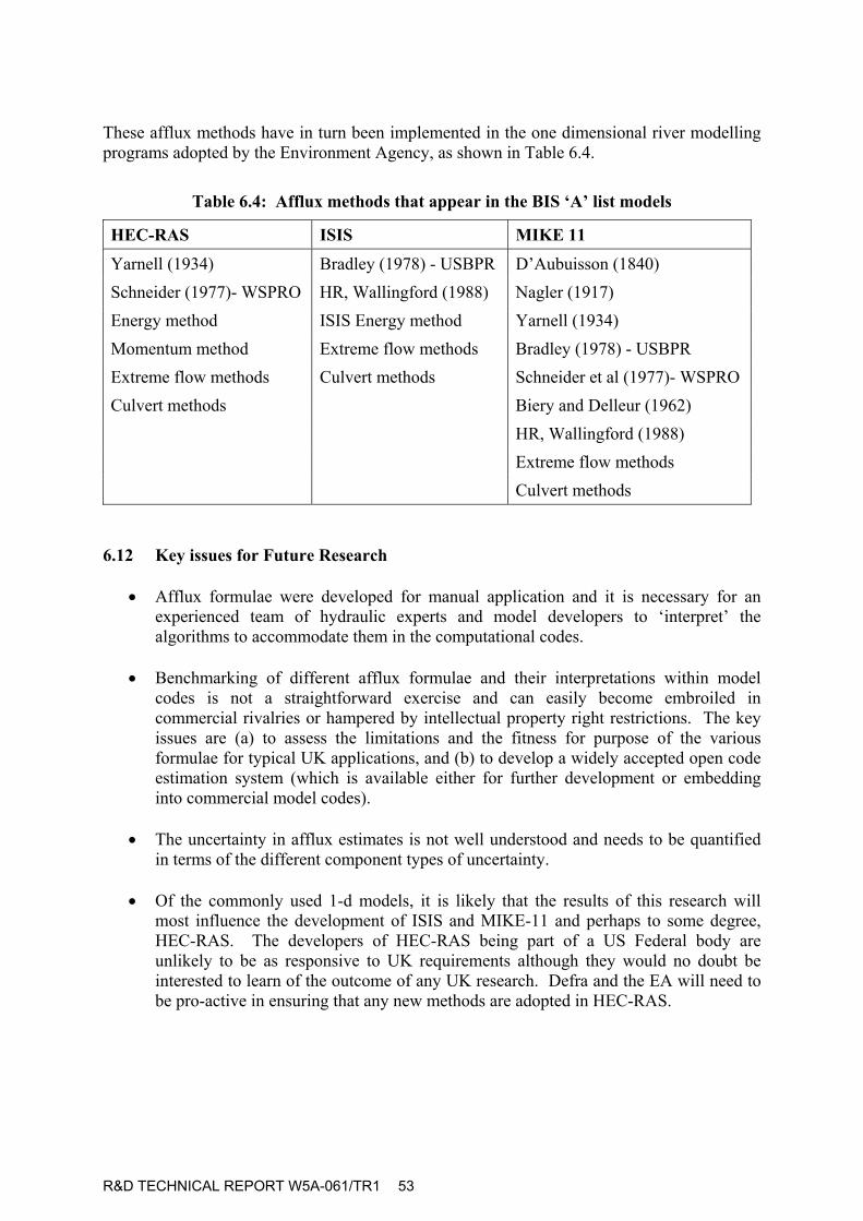
These afflux methods have in turn been implemented in the one dimensional river modelling programs adopted by the Environment Agency, as shown in Table 6.4.
Table 6.4: Afflux methods that appear in the BIS ‘A’ list models
HEC-RAS ISIS MIKE 11
Yarnell (1934) Bradley (1978) - USBPR D’Aubuisson (1840) Schneider (1977)- WSPRO HR, Wallingford (1988) Nagler (1917) Energy method ISIS Energy method Yarnell (1934) Momentum method Extreme flow methods Bradley (1978) - USBPR Extreme flow methods Culvert methods Schneider et al (1977)- WSPRO Culvert methods Biery and Delleur (1962)
HR, Wallingford (1988) Extreme flow methods
Culvert methods 6.12 Key issues for Future Research
• Afflux formulae were developed for manual application and it is necessary for an experienced team of hydraulic experts and model developers to ‘interpret’ the algorithms to accommodate them in the computational codes.
• Benchmarking of different afflux formulae and their interpretations within model
codes is not a straightforward exercise and can easily become embroiled in commercial rivalries or hampered by intellectual property right restrictions. The key issues are (a) to assess the limitations and the fitness for purpose of the various formulae for typical UK applications, and (b) to develop a widely accepted open code estimation system (which is available either for further development or embedding into commercial model codes).
• The uncertainty in afflux estimates is not well understood and needs to be quantified
in terms of the different component types of uncertainty.
• Of the commonly used 1-d models, it is likely that the results of this research will most influence the development of ISIS and MIKE-11 and perhaps to some degree, HEC-RAS. The developers of HEC-RAS being part of a US Federal body are unlikely to be as responsive to UK requirements although they would no doubt be interested to learn of the outcome of any UK research. Defra and the EA will need to be pro-active in ensuring that any new methods are adopted in HEC-RAS.

R&D TECHNICAL REPORT W5A-061/TR1 54