A IffCONF-781108 - -

1978DOE STATISTICAL SYMPOSIUM

November 1-3,1978Sandia Laboratories

Albuquerque, New Mexico

Sponsored by the Department of Energy

Prepared by

OAK RiDGE NATIONAL LABORATORY

Oak Ridge, Tennessee

Operated by UNION CARBIDE CORPORATION for the DEPARTMENT OF ENERGY

CONF-781108' *Distribution Category UC-32

1978DOE

STATISTICALSYMPOSIUM

- NOTICE -Ifck nport « M pnptied as an account of wmfctpotuond by the United Suui Government. NSMMT * cUnited States not die United States DapvtSMt ofEnergy, nor any of tftek cmptoyw, aor any of tiwircontnctpjs, Mibcontncton, or thtk miwiicyni, — I M Iany warranty, txpttu or impUed, or amtmr my l f fd(Utility or rMponatoiity for the accuracy, compblmMict 'jwfHbKK of any infonnation, appaniw, prodvct orproccai diKkwed, or Kpmeaa that Ms we would notinrrmr privately owned rights.

November 1-3,1978Sandia Laboratories

Albuquerque, New Mexico

Compiled and Edited by

Herbert T. Davis, Sandia LaboratoriesRichard R. Prairie, Sandia Laboratories

Tykey Truett, Oak Ridge National Laboratory

Sponsored by the

Department of Energy

Date Published: July 1979

Prepared by

Oak Ridge National LaboratoryOak Ridge, Tennessee

Operated by Union Carbide CorporationContract No. W-7405-eng-26

CONTENTS

PREFACE

INVITED PAPERS

Growing Trees to Analyze High-Dimensional Data, L. Breiman 3Energy Information Validation, L. E. Moses 31

RESEARCH PAPERS

Ranking Energy Policy Alternatives in a Partially InformedPopulation, N. S. Urquhhrt and C. Eastman 53

Statistical Design and Analysis of Power Plant EntrainmentStudies, R. D. Small; T. Capizsi, and L. E. Sage 66

Exponential Responses with Double Exponential MeasurementError — a Model for Steam Generator Inspection,R. G. Easterling 90

Redundant Systems Subject to Simultaneous Failures,L. R. Abramson Ill

The Use of Semi-Controlled Experiments in the Analysis ofResidential Energy Demand, L. S. Mayer 126

Improving the Reliability of Econometric Models,R. E. Welsoh 146

Estimation of the Amount of Exposure to an EnvironmentalClastogen Using Human Cytogenic Dosimetry, E. L. Frameand R. J. DuFrain 169

Geostatistical Methods in Lignite Reserve Estimation,H. D. Tolley and J. R. Alldredge 193

Stochastic Mirror Errors — Computation of Optical ConcentrationDistributions and Variance Distributions of SolarReceiver/Boilers, J. D. Reiohert . . . . . 209

Dynamic Analysis of Nuclear Safeguards Systems, J. R. Wilson^D. M. Rasrmson, and F. H. Tingey 229

PROBLEM PRESENTATIONS AND DISCUSSIONS

Multivariate Statistical Methods Applied to PostnatalMeasures of Neuromuscular and Behavioral Developmentin the Rate Exposed Prenatally and Neonatally toLow-Level Electric Fields, R. L. Busehbom andP. G. Doctor 255

Problem Discussion 267

iii

Page

Analysis of Proposed Transient Overpower Experiments,K. Campbell and D. Hurd 274

Problem Discussion 287Some Statistical Aspects of the Cleanup of Enewetak Atoll,

M. G. Barnes, J. J. Giacomini3 and H. N. Fviesen 296Problem Discussion 319

SUMMARY AND CONCLUSIONS SESSION , . . . 325

LIST OF ATTENDEES 335

iv

: PREFACEi

lThe 1978 DOE Statistical Symposium, hosted by Sandia Laboratories,

was held in Albuquerque, New Mexico, November 1-3, 1978. The 112

attendees included people from DOE, industry, and the academic community.

Previous symposia were held at Los Alamos, New Mexico; Oak Ridge,

Tennessee; and Richland, Washington.

The program for the fourth symposium, which followed the format of

the previous three, included ten technical papers and three problem

presentations with discussions. As can be seen in the Proceedings, quite

a wide range of energy-related topics were covered. Invited papers were

presented by Leo Breiman and Lincoln Moses. An additional feature was

a follow-up on the status of three problems presented at previous

symposia. The program also included four informal discussion sessions

on the topics of risk analysis, model validation, safeguards, and health

and environmental effects. The success of these informal sessions,

inaugurated at the 1977 DOE Symposium, led the Symposium's Steering

Committee to recommend that the present "formal" problem sessions be

supplanted by workshops. This recommendation was accepted by the

attendees at the conclusion of the 1978 Symposium and will be implemented

at the 1979 Symposium to be hosted by ORNL and held at Gatlinburg,

Tennessee.

We feel that achievement of the symposia goals of furthering

communication among DOE-affiliated statisticians and promoting the cause

of professional statistics in helping to solve the nation's energy

problems were advanced by the fourth symposium. We wish to thank all

attendees and participants, and we confidently look forward to future

symposia.

Invited Papers

GROWING TREES TO ANALYZE HIGH-DIMENSIONAL DATA

Leo BreimanTec\uology Service Corporation

Santa Monica, California

-•-."^..^.(r^v-rrjfc^rrrrrTi-rr/a^^

I. INTRODUCTION

It has been my good fortune, over the last few years as a consultant

at Technology Service Corporation, to work on a number of interesting

problems such as

• Radar Profile Classification

t Spoken Word Classification

t Prediction of Air Pollution Levels

• Factors Contributing to Delay in Court System

• Classification of Chemical Mass Spectra

These are all prediction or classification problems. What makes them

particularly interesting is the shape of the data. That is,

e Moderate to high dimension (6 to 1000)

• Non-linear and generally non-additive

• Mixed ordered and unordered variables

• Non-standard, i.e., variable dimensionality

The goals of the analysis were:

• Reduction of dimensionality

• Extraction of key variables

• Accurate prediction/classification

• Understandabiiity

The last issue, that of understandability, has not beer; stressed enough in

statistics. The statistician, in analyzing data, usually works with other

specialists in the field. For instance, I am constantly interacting with

chemists, meteorologists, radar engineers and so on. In order to carry

forward the scientific investigation in which the data analysis was

embedded, the results of the analysis must be easily interpretable and

understandable to non-statisticians. Since more is required of the

analysis than accurate prediction or classification, I generally tend to

thiik of it as the problem of extracting information from high dimensional

data.

In this problem of effectively extracting information from large high-

dimensional data sets,most of classical statistics is not applicable, and,in

fact, was not designed for this problem. Its growth was restricted by the

technology of hand computation or desk calculator, and by limitations of

data gathering technology. But the critical foundation ideas of statistics

remain in force: replicability of conclusions under independent reruns;

questions of bias; and the size of random errors.

The data handling capabilities of the computer are opening up new

directions for statistical thinking. Considering the computer as nothing

more than a super-fast desk calculator puts a straitjacket on our thinking.

It reminds me of the thinking that said "A gas engine is nothing more than

a more powerful horse," and put the engine between the poles of a carriage.

But this "more powerful horse" ended up producing a profound and revolu-

tionary change in our transportation system and in the character of our

cities and lives. Similarly, present day packaged statistical programs are

a transitional phenomenon, like a gas engine driving a buggy.. The use of

the computer makes feasible methods of analysis simply unthinkable a

generation ago.

In fact, many of the most recent effective data-analytic techniques

have been designed by computer-oriented nonstatisticians. I've had the good

luck to work with two such people: William Meisel, at Technology Service

Corporation, whose background was in computer oriented pattern recognition

and Jerome Friedman, a physicist turned data analyst in charge of the

computer facility at the Stanford Linear Accelerator Center. Our work

together has been an interesting experiment in bilingual education.

What tools are available for extracting information in prediction/

classification situations? Over the last few years, I've used a variety

of methods. Here is a brief review with some comments on their advantages

and disadvantages.

Classical

Multilinear regression

Stepwise variable selection

Best subset selection

Parametric nonlinear regression

Linear discriminant analysis

Stepwise variable selection

The limitations of these methods are well known, but they are widely and

sometimes inappropriately used simply because of their availability.

Nonclassical

Use of interpoint distances

k nearest neighbor classification and regression

Kernel density estimates for classification and regression

The major advantage of these methods is that the only assumption

necessary regarding the shape of the classification-regression surface

is some weak form of local smoothness. There are serious disadvantages.

The resulting analysis has poor understandability. The entire data set

must be stored for prediction or classification of future objects. The

methods work only on data types restricted to ordered variables with

8

fixed dimensionality. The sensitivity to choice of distance measure is

largely unknown.

Nonclassical

Piecewise linear or piecewise polynomial approximations

• Spline fits - dimension limited.

• Piecewise linear data-directed fitting-

unlimited dimensionality

Research in discontinuous piecewise linear fitting was reported in

Breiman and Meisel [1], continuous piecewise linear fitting in Meisel and

Collins, [2], Again, the only assumption needed regarding the shape of the

regression surface is local smoothness. These methods work best on ordered

data, but can also be used on mixed data types. The major disadvantage is

poor understandability.

Neither of the above methods is an effective information extractor.

Even after finishing an analysis, very little is learned concerning the

structure of the problem, the relation between variables and what is

significant. For this reason, we have recently started work on growing

and pruning trees.

II. GROWING OUR FIRST CLASSIFICATION TREE

The first situation in which we grew a tree was a classification

problem we were working on about 5 years ago. It is a good example of

why a tree-structured approach was an appropriate and logical procedure.

The problem was to classify ships by means of their radar range profiles

We had data from 6 ships, with twenty profiles per ship taken at a variety

of angles. You can think of the range profiles as being continuous wave-

forms (see Figure 1) with the maximums corresponding to certain structural

features of the ships. As the angle of the radar picture changed, we

found that the locations of the local maximum of the profiles relative to

the length of the ship remained fairly stable. Therefore, as a first step,

we reduced dimensionality by extracting the locations of all local maxima

in the profiles. The resulting data set had a non-standard structure with

dimension varying from 1 to 12. We were left with the problems of devising

a multiclassification method that would deal with this data structure. Our

solution was to grow a tree. A tree consists of nodes and splits of nodes,

where a node N = a subset of the data. To get splits of the nodes, a set

Q of yes-no questions is defined on the independent variable space. This

set Q generates a set S of splits s of the node N into N.and NRJ the left

and right descendent nodes (Figure 2).

Figure 2

10

In general, the set of questions Q is quite numerous. To select a

single split from the many alternative possible splits, a "goodness-of-split"

criterion D(N,s), is defined for each node N and split s. A "good" split

is a split which effectively separates classes.

EXAMPLE OF A VERY GOO.D SPLIT

Define the "best" split to be that split which maximizes D(N,s).

In the ship problem, the profiles were all normalized to be on the

interval £0,1]. The set of questions Q were all questions of the form:

Does the profile have a local maximum in the interval [a,b]? The values

of a, b were taken to range from 0 to 1 in steps of .01 with a<b. This

gave a total of about 5000 questions. The tree growing procedure

proceeds as pictured in Figure 3 .

11

Figure 3. Tree Growing

SEARCH THROUGH 5000 SPLITS, FIND BEST SPLIT

BEST SPLIT

SEARCH AND FIND BEST SPLIT SEARCH AND FIND BEST SPLIT

SEARCH AND FINDEST SPLIT

STOP

The growing stops at nodes where there are no effective splits. These are

called terminal nodes.

12

So far, we have not yet specified the goodness-of-split criterion

vhen to stof

probabilities as

and when to stop. If node N contains m- of class j. defined node classJ

The impurity of a node I(N) is defined to be a function of the node class

probabilities with the general properties;

I(N) = 0 if max (UN) = 1

I(N) = maximum when Q-j = Q« = ...

Originally we took

I(N) = - V (UN)log Q.(N) ,J

simply because this function had the right overall behavior to serve as an

impurity function. There is nothing particularly unique in this functional

form that makes it the "best" one and we have since experimented with and

switched to other impurity functions.

The probability P(N) of falling into N is defined as

P(N) = m/n,

where m is the number in node N, and n is the original sample size. Now

take the overall impurity of a tree I(T) as

KT) «Nt

where the sum is over all terminal nodes N..

13

With this notation, our goodness-of-split and stopping goes as

follows: Take any unsplit node N in the current tree T. Consider

a split s of N. The new tree T1 has impurity

I(T') = ^ I(Nt)P(Nt) * I(NL)P(NL) + KNR)P(NR)Nt-N

The decrease in impurity of the tree due to the split is

- I(T') = I(N)P(N) - I(NL)P(NL) - I(NR)P(NR)

This depends only on the node N, and the split s. Define the goodness-of-

split s of node N to be this decrease, i.e., put

D(N,s) -I(N)P(N) - I(NL)P(NL) - I(NR)P(NR)

Our original stopping rule was of the from; set a threshold 6 and make

N terminal if

max D(N,s) <. B.s

Select B by trial and error.

Now that we've grown a tree, how does it get used on future samples?

Decide the class character of each terminal node by the plurality rule.

That is, if N contains m. of class j, then call N a j class node if

m. = max m..Jo j J

As a very important addition, there is a simple estimate of the probability of

correct classification given that object falls into node N. Recalling that

the class probabilities in N are given by

14

estimate the probability of correct classification given N by

PJN) = maxc j

When a future object is passed through tree, if it falls into terminal

node N, then the output is

PROBABILITY OF CORRECTCLASSIFICATION CLASSIFICATION

By plurality PC(N)rule in N

There were some notable advantages to this tree growing approach.

Powerful use was made of conditional information. By this is meant that

at each node, the best discriminating split is found in terms of only the

population in that node. For instance, suppose the first question is

"local maxima in [.35, .53]?" For the ship profiles that answered yes, the

most discriminating location of another local maxima is the interval

[.07, .17], while for those that answered no, the best discriminating

interval is [.82, .90]. The results of the analysis had an almost trans-

parent understandability in terms of the structural features of the ships

involved. The classification algorithm for future objects was simple and

efficient consisting of storing a list of around 30 short questions with

yes-no answers.

There were also some r.otable disadvantages. Of course, growing this

tree was computationally expensive. At each node a search was made through

5000 questions to find the best split. Even so, the computational expense

was and is only a minor disadvantage. The most serious concern is the

possibility of considerable overfitting and upward bias. In multilinear

15

regression, for example, one is doing an optimization { minimization)

over a small number of parameters and there are explicit theoretical

results which correct for the bias caused by the optimization. In tree

growing, the best split among a large number of splits is selected at each

node. The amount of bias "introduced by this degree of tailoring the

procedure to the data is not yet theoretically assessable. Our experience

is that it can be dangerously large. The problem of dealing with this

bias is at this point the most important issue in effective tree growth.

We've made some progress that I'll report on later.

III. GROWING REGRESSION TREES, ATD-CART

After growing our ship classification tree and talking to John Hartigan

about it, he told me about a ^/ery simlar regression algorithm called AID

(Automatic Interaction Detector) that had been developed at Survey Research

Center, University of Michigan, some years before,[3]. AID is a tree-

structured regression algorithm, that operates on standard data structures

(\» ^ ) » with the independent variable having fixed dimension,

X =

with either ordered or unordered variables. At each node N, the set Q of

questions is of the form:

Is X. <. x? (Xi ordered)

or

Is Xi e {j-|,...,q } c{l j} ? (Xj unordered taking values in {!,...»J})

16

The algorithm searchs over all coordinates X,,...,XM for the best split.

For ordered variables, it serached over all possible split points. For

unordered variables, over all possible subsets of values. Actually, the

original AID algorithm restricted the search to only a small number of speci-

fied split points on the ordered variables. The upgraded version (CART) we

use at Technology Service Corporation does the unlimited search. The poten-

tial number of splits can be large. For example, with 1000 data points, and

20 ordered variables (and no ties), there are 20,000 potential splits at the

root node.

The goodness-of-split criteria in AID is similar in spirit to that

used in our classification tree. Look at Figure 4 below.

Figure 4

From a regression point of view, what we want of a good split s is that it

puts high Y. values into one node, low Y^ values into other node. For

instance, s is good if it gets all the high Yk values off into the right

node NR, and the low values into the left node N, . Another way of

-™.-;:*^

17

putting this is that we want tha variances of the two descendent nodes to be

reduced as much as possible form the variance of the parent node. Therefore,

define the impurity of a node by

I(N) = a2(N),

where a2(N) is the sample variance of the YK values in node N. Define

the impurity of a tree by

NtI(Nt)P(NJ ,

and, as before, take the best split to be the one which reduces the

impurity the most.

There is another interesting way of looking at AID. As an example,

suppose we have two independent variables, X,, X« both taking values on

[0,1], Geometrically, then, the independent variable space is the unit

square. Say, for instance, that the tree turns out to look like Figu*e 5

below;

Figure 5

STOP STOP

18

Another way of picturing this is that we have cut up the independent

variable space into the rectangles of Figure 6 be1ov

Figure 6

v ALTERNATE DIAGRAM

.6

#2

T(2)

#1T( l )

#3

Y (3)

.75

In general each terminal node corresponds to a rectangular region in

independent variable space. In each such region N, take the predictor of

Y to be the sample mean T(N). This gives ? multidimensional histogram -

like prediction surface. The mean RSS (residual sum of squares) of the pre-

dictor is

where I(T) is the tree impurity defined above. The goodness-of-split

criterion can be given an alternative form;

D(N,S) = a2(N)P(N) - a2(NL)P(NL) - a2(NR)P(NR)

*C5S(N) - SS(NL) - SS(NR)]/n

19

Therefore, the AID criterian selects the split which gives the largest reduction

in residual sum of squares, using predictors which are constant across

rectangles. This is analagous to ordinary linear regression which minimizes

the residual sum of squares using the class of linear functions as predictors.

CART (classification and regression trees) is a general purpose program

for growing and pruning trees developed at Technology Service Corporation

in collaboration with Charles Stone. It includes an upgraded version of

AID. It has been extensively used on a wide variety of problems such as

air pollution analysis, gas mileage analysis, and model diagnosis. It is

a widely used program among the scientists at TSC. The popularity is largely

due to its understandability, and to the simplicity with which the results

of the analysis translate into the physical meaning of the problem. For

exampla, Figure 7 is the result of growing a tree for data with the dependent var-

iable being the daily maximum Los Angeles N02 reading. The independent variables

consist of various meteorological measurements. Ten meteorological variables

were included, but only five were found by the algorithm to give the opti-

mizing splits. This method shares with all regression methods the problem

that some variables may be masked by others. For this reason, we have

output supplementary to the tree diagram which examines the splits in more

detail. The standard deviation is computed for each node population.

For the terminal nodes this gives quick confidence interval statements for

the predicted values using the node means. However, the estimated standard

deviations may be seriously biased toward the low side. In regression, as

in classification, the issue of bias is critical.

20

Figure 7, N02 Analysis

N- 1-2SSR- 1S.Z7S- 9.25

LfiXISHI.

N- 195n- 17. ms- e.t3

LflX9TP14

iN 3 1n- 2i.c.S- 10.25

PRESGRflO

N- ..a N- 551

LflXIBHi*3Ht *•»#»«**

<• 106.03 > 105. 12. 12.00 2100.00 > 2100.00N-

12N- 222M- 28.009- 10.23

LHX0VZ7

N-

RflNK-

N- 15SMM t9 HOO H.XO

RflNK- 7

N-

*»»»»»»*•»

8.

Mm ^ P

S- 11DflYLENG

2871

N-

RfiNK-

191

11.40N- 19M- 15.05S- 11.38RSNK- 1

N" 9

RflNrt- ' 3

Abbreviations:

LAX1BH4 LAX morning inversion based height

LAX9TM4 LAX morning y50 mb. temperature

LAXPV27 LAX v i s i b i l i t y a t 7 A.M.PRESGRAD C o a s t - t o - d e s e r t pressure grad ient a t 7 A.M.DAYLENGT Number o f d a y l i g h t hours

N Nods p o p u l a t i o nM Node meanS Node standard deviation

21

IV. FURTHER WORK ON CLASSIFICATION CRITERIA

The two-class classification problem can be transformed into a

regression problem by putting

0;k point in class I

1; k**1 point in class II

If we carry out such a transformation, then in node N, with class pro-

babilities Q-j(N), Q2(N), using the AID definition of node impurity, we get.

I(N) = o2(N) = Q^N) Q2(N)

= PC(N)(1-PC(N))

Originally, I though that the above definition of node impurity in the

context of a classification problem was artificial and unsuitable. For

instance, in regression, the universally accepted figure of merit is percent

of variance explained (PVE) or not explained (PVNE). AID works directly to

minimize PVNE since the tree impurity is proportional to PVNE. In this sense,

the definition of impurity and goodness-of-split are directly related to the

goal of prediction accuracy. In classification,the universally accepted figure

of merit is the proportion of items misclassified. But tree impurity defined

using P (1-P ) has no apparent connection to the proportion misclassified,c c

If we want a direct connection, we could take

I(N) = 1-PC(N),

then,

= £ (l-Pc(Nt))P(Nt)Nt

= Proportion of items misclassified

22

Why not use this definition, instead of the more artificial expressions

such as P.O-PJ, or the entropy measure we originally used?

There two good reasons. The first, and most important is that the

criterion 1-P is degenerate. Look at the example given in Figure 8.

Figure 8

The number misciassified with both splits decreases from 400 to 200. Both

splits will give the same criterion value. In fact,the 1-P criterion will

often select many splits of a given node as being equally "best". Are the

two splits above equally good? In most applications the 2 n split is clearly

preferrable. It results in one node, containing half of the population,

with perfect classification. In the 1 split, the probability of correct

classification in both descended nodes is 75%, certainly not high enough to

write home about.

When we formalized the reasons why 2 split above is preferable with

a model, we came to the following conclustion: all "reasonable" I(N)

functions in 2-class problem are functions of P_(N), satisfyingc1. <{>(Pc) is decreasing in

2. $(P ) is concave in P

3. *(1) = 0, <j>'0/2) = 0 .

23

The simplest polynomial satisfying these three conditions is

<j>(P ) = P (i_p ) (AID cr i ter ion)c c c

but another function that also satisfies the conditions is

c ) = -Pc lag Pc - (1-Pc)log(l-Pc)

We have done some preliminary experimentation that indicates that the tree

structure is not too sensitive to the form of <|>(PC) used.

V. GROWING A CHEMICAL SPECTRA TREE

A recent project had as its purpose the construction of an algorithm

to classify compounds as containing Or not containing chlorine by looking at

their mass spectra. A mass spectra graphically looks like Figure 9.

Figure 9

MASS SPECTRA:

1 -•

4 5 6 MolecularWeight

For our purposes, the mass spectra of a molecule is a vector of non-

negative coordinates whose dimensionality is approximately equal to the

24

molecular weight. We used the EPA data base of about 30,000 spectra with

molecular weights rangining from around 50 to 1000.

The class of questions Q that were addressed to each spectra were

similar to questions of the type

Do you have a non-zero peak at K, or K~?

Do you have a peak of height > h at K?

The resulting tree gave 93% correct classification with 29 terminal nodes.

Having such a large original data set, we could afford to store away 10,000

spectra as an independent, test set. The estimated percent of correct

classification based on the learning set was only about 1% higher than the

test set results.

The algorithm is currently being put up on the EPA computer system.

Its output gives both the classification of the compound and the estimated

probability of correct classification

Sample Output

CLASSIFICATIONPROBABILITY OF

CORRECT CLASSIFICATION

Compound #1 CHLORINE .97

Compound #2 NO CHLORINE .65

etc.

25

The probability of correct classification is an important byproduct of this

classifier. If it is high, the questioner will be inclined to accept the

classification. But if it is close to .50, they should consult a trained

chemist for a 2n opinion.

To summarize, growing trees have these advantages.

1. Powerful use of conditional information for

variable selection.

2. Understandability and ease of interpretation for

nonstatisticians.

3. Produces simple rules for prediction or

classification.

4. Yields immediate confidence statements for

predictors.

Growing Trees have these disadvantages:

Somewhat computationally inefficient

1. Can give very biased overall results.

2. Can give biased variable selection.2

3. Can give biased estimates of node a or P .

VI. DEALING WITH OVERALL BIAS THROUGH PRUNINGAND CROSS VALIDATION

We have been exploring a method for estimating the overall bias in a

tree, and for producing a good-sized tree. By this, we mean a tree that

is neither so large that it overfits the data, or so small that it is not

extracting relevant information.

For a tree T, let

|T| = Number of terminal nodes.

26

Define the cost of a tree, C(T), to be

C(T) = I(T) + a | T | .

where a is a preselected number. One part of our procedure is Tree Pruning,

which goes in these steps:

1. Set the split threshold 6 very low and grow a large tree

V2. For each value of a , there is a subtree T c T which minimizes

C(T) = I(T) + a |T|. Call T the optimally pruned tree for cost a

per terminal node.

Notice that as a increases, the optimally pruned trees {T ] shrink upward

to the root node.

The second part is Cross Validation. We illustrate this for a regression

tree. The data set is divided at random into 10 subsets of equal size

S1, »si0" Deflne tne "'th learning set L., i = l,...,10 to be all data

except the set S.. Using the i learning set and a low B threshold, we

grow a large tree T • Prune the original large tree T upward to T and

each learning tree upward to T • Using the tree T ^ 1 ' as a predictor,

run the set S. through T ', and compute the percent of variance

explained. Denote this by PVE (i,a). Define

10 /\

SD

As & increases from zero, PVE(a) grows, reaches a maximum, and decreases.

We select the tree for which PVE(a) is a maximum. A similar procedure

27

is used in classification, by estimating the percent of correct classifi-

cation through the cross validation method.

Our experiments on simulated data have given encouraging results

regarding the accuracy of pruning-cross validation. Table 1 contains part of

the CART output for simulated two-class data in which we also generated a

large independent test set and ran it through the trees to get accurate

estimates. The various sized trees are the result of the upward pruningrdoperation. The 3 column gives the percent of correct classification

estimated by cross validation, and the underlined value denotes the tree

size selected by the cross validation. The 2n column gives the percent

of correct classification estimated without using cross validation, and

the last column gives the test set results. Use of the tree estimates

without cross validation or an independent test set are seen to give an

overly optimistic view of the classification accuracy.

TABLE 1

NUMBER OFTERMINAL NODES

23.17.13.7.6.5.4.3.2.

CART

% CORRECTLEARNING DATA

100.098.597.094.09O"89.084.578.567.0

OUTPUT

% CORRECTCROSS-VALIDATION

78.5 +79.5 +79.5 +83.0 +8 0 3 +76.0 +76.0 +69.5 +59.5 +

2.82.82.82.12.72.42.43.31.6

% CORRECTTEST SET

79.380.081.381.98TT9"78.077.372.363.5

28

VII. THE PROBLEM OF BIASED VARIABLE SELECTION

In brief, the problem Is that the more splits possible on a variable,

the more it will tend to get chosen regardless of predictive capability.

For example, for an unordered variable, taking on 20 values, there are

about 500,000 possible splits. I have made some theoretical computations,

with the conclusion that for large sample size, a pure noise unordered

variable with >8 values will have a better split than a pure noise

continuous variable, and conversely with <8 values. We are currently

experimenting with one possible solution that consists of a within-node

cross validation. But the results are not completely satisfactory yet.

Another related problem is in the biased estimates of a or P at terminal

node. This is connected with problem discussed above and headway is hoped

for using within-node cross validation.

VIII. CONCLUSION

Tree structures are being used by statisticians and non-statisticians

alike in diverse applications. A recent(July 1978)issue of the Western

Electric Engineer outlined their process characterization analysis package

(PCAP) of which the two central elements are a classification tree growing

algorithm similar to the one used on ships, and a regression tree growing

algorithm similar to AID. The growing and pruning of trees for regression

and classification is an idea whose time has come. In fact, if William S.

Gosset were currently working in a brewery, we might very well see a publi-

cation contianing the following diagram

29

STUDENTS TREE

WaterType #1 % Barley > ?

REFERENCES

[1] L. Breiman and W. W. Meisel "General estimates of the intrinsic- variability of data in nonlinear regression models" JASA, June 1976,

Volume 71, No. 354, pp. 301-307.

[2] W. S. Meisel and D. C. Collins "Repro-modeling: an approach toefficient model utilization and interpretation" IEEE Trans, on Systems,Man, and Cybernetics, July 1973, Vol. SMC-3, NO. 4, pp. 349-357.

[3] J. A. Sonquist, E. L. Baker, J. N. Morgan "Searching for Structure"1973, Survey Research Center, Institute for Social Research, Universityof Michigan, Ann Arbor, Michigan.

NOTE: There have been a number of papers published in various fieldsover the last few years on tree structured methods similar to thosediscussed in this paper. We are collecting these and intend to compilea complete bibliography.

ENERGY INFORMATION VALIDATION •

A STATUS REPORT

Lincoln E. MosesEnergy Information Administration

Department of EnergyWashington, D.C.

ENERGY INFORMATION VALIDATION

A STATUS REPORT

The world oil supply crisis and price escalation of the 1973-74period brought energy issues to a new prominence, and vividly exposedanother kind of shortage. There was a shortage of information —•especially of credible information — about petroleum and the petroleumindustry. Hard numbers, soft numbers, changing numbers, conflictingnumbers added to the frustrations of the accommodations made to a four-fold rise in the world price of oil.

By summer of 1977, when the Department of Energy was about to beborn, plans for the new Department called for an Energy InformationAdministration, and it was to include a part then named the Bureau ofEnergy Data Validation. That organization was slated to have about 30%of the staff and 20% of the budget of the EIA. That was the plannedorganizational response to the lack of validity of energy data. When onOctober 1, 1977, the Department came into being, one of its three .principal branches was the Office of Energy Information Validation(OEIV). It was much smaller than 30% of the organization — more like5% at the end of that first year, but clearly expected to grow as plansbecame clearer and firmer.

In the early months of the Department, the general charge of OEIVto address the credibility of energy information began to resolve itselfinto a group of rather more specific tasks. I shall now take thesetasks up one by one.

Verification of Information Submitted by Respondents.

The matter was put vividly by the author of the progressive incometax, Sir Josiah Stamp, when he said:

"The Government are very keen on amassing statistics. Theycollect them, add them, raise them to the nth power, take the cuberoot and prepare wonderful diagrams. But you must never forgetthat every one of these figures comes in the first instance fromthe village watchman, who just puts down what he damn pleases."

Verification of the accuracy of submitted information lies at theheart of the credibility problem. It has several aspects. Has therespondent given us the same number that is in his records? Is thatnumber an honestly prepared one? Even if it is honest, is it accurate?These questions are readily illustrated in the Oil and Gas InformationSystem (OGIS), a survey that will call on oil and gas producers todisclose rheir annual production and reserves by reservoir (or for somerespondents by field). For the OGIS, we quickly come to these questions:(1) Has the respondent told us what he actually carries on his books?(2) If so, is that number a reasonable result considering the geophysicaland production data from which it was derived? (3) Do the reserve

33

34

estimation methods commonly used tend systematically to result innumbers that are too high (or too low)? The OEIV will investigate thefirst question by verifying submitted returns against operator recordsfor a sample of respondents. For a sub-sample (smaller, because ofexpense to the Government and burden to the respondent), OGIS willcompare reserves to the supporting geophysical and production data withan eye to appraising the reasonableness of the respondents' own reservefigures. The third level of verification, examining the validity of theestimating methods themselves, may become a research priority of OEIV,or it may not. But that level of validation of energy information is anoption which will sometimes become a necessary responsibility forparticular data systems.

Checking the Integrity of Data Collection Systems.

Here, as in all of the remaining functions that I shall list, OEIVis checking not only the respondents but also parts of EIA. There aremany steps in the path from initiating a data collection form to pub-lishing a table — and Murphy's Law applies throughout that long path.For what reasons is this form being launched? Who needs the informationsought? For what purposes? Will the information serve those purposes?How accurate must it be? How current? Is the instrument clear andunambiguous? Are the definitions present, correct, and clear? Howabout the instructions? Does the form go to respondents who have theinformation to answer the items? Is the frame satisfactory? How aboutthe sampling plan? Is the response rate high enough? Are the non-respondents sampled? Adequately? Are the audit checks satisfactory?What about imputations? Are all these steps adequately documented? Adraft document which captures these and other issues, in a more opera-tional form appears as Appendix I to this paper.

Participating in new Systems Establishment.

We early saw that it could hardly be wise to let validation be onlya retrospective process; that could allow that in January we wouldestablish some system with design flaws and delay until December theiridentification and correction. So, OEIV is a participant in the energyinformation forms clearance process which EIA conducts for the Depart-ment of Energy. Further, OEIV sometimes participates more fully in thedesign phase than merely by taking a part in the forms clearanceprocess. An important example is the OGIS for which the interaction wasbroad and searching. Both the form (and its instructions) and the frame(and sampling plan) benefited greatly from the collaboration between thetwo groups.

"Rolling Review" of all Systems.

We early set this function as one which we should have in EIA —and assigned it to OEIV. There is a tendency for data collectionsystems to become immortal. When a form has outlived its usefulness,then both the Government and the respondents are suffering from wasted

35

effort. The "rolling review" idea provides that every system get ' lewassessment on some regular cycle, probably every four or fivr is.It has been likened to a "sunset law" for data systems. Prest "MBforms clearance procedures already provide limited term rather indefiniterenewals. We view that policy as a call for just the kind of systematic,searching agency review that we embody in the "rolling review" concept.

Validation of Models.

In 1883 Mark Twain wrote a passage in Life on the Mississippi whichposes the problem of model validation. He had just described howoccasionally the meandering river would break a new channel replacing alarge bow by a "cut off." He summed up in these words:

"Therefore, the Mississippi between Cairo and New Orleans wastwelve hundred and fifteen miles long one hundred and sixty-sixyears ago. It was eleven hundred and eighty after the cutoff of1722. It was one thousand and forty after the American Bendcutoff. It has lost sixty-seven miles since. Consequently itslength is only nine hundred and seventy-three miles at present...

"Please observe: In the space of one hundred and seventy-sixyears the Lower Mississippi has shortened itself two hundred andforty-two miles. That is an average of a trifle over one mile andone third per year. Therefore, any calm person, who is not blindor idiotic, can see that in the Old Oolitic Silurian Period, just amillion years ago next November, the Lower Mississippi River wasupwards of one million three hundred thousand miles long, and stuckout over the Gulf of Mexico like a fishing rod. And by the sametoken any person can see that seven hundred and forty-two yearsfrom now the Lower Mississippi will be only a mile and threequarters long, and Cairo and New Orleans will have joined theirstreets together, and be plodding comfortably along under a singlemayor and a mutual board of aldermen. There is something fascinatingabout science. One gets such wholesale returns of conjecture outof such a trifling investment of fact."

Modern day forecasting models Involve many — often thousands — ofassumed or computed numerical inputs. In addition they may accept avariety of "scenario" variable's, which are assigned hypothetical values.Then more or less elaborate and nontransparent algorithm are applied,resulting in outputs. Questions abound: How accurate are the inputs?How reasonable are the theories that are captured in the algorithm? Dothe algorithms actually do what they purport to do? Because not all thecomponents can be correct (there may be scores of thousands of them),how important are inaccuracies to the results? The phrase "validationof models" is brief and conceals an enormous complex of questions.Early steps will be to choose for study particular questions that can beusefully and effectively addressed, to identify important issues, theunderstanding of which can be usefully enlarged by research, and tomeanwhile keep an eye on documentation of, and open access to, EIA's

36

models. A related kind of action is to maintain a tickler file of EIA(and other) forecasts with a view to comparing actual outcomes with theforecasts as the future unrolls. (Of course, we must note that suchcomparison is often impossible. Forecasts may relate to alternativeprice or policy scenarios of which at most only one can ever occur, andoften none will.)

Validation of Publications.

To many people, EIA will be known only through its publications andreports of them. We must have a systematic concern for the integrity ofthose publications. The bulk of that responsibility is borne by theoriginating offices, with much reliance on internal (and sometimesexternal) review. But the charter of 0E1V must reach as far aspublication in order to embrace fully the original goal of assuringcredible energy information. The process of "validating publications"will attend to documentation of stated results, inclusion of sufficientwarnings, fairness of graphical presentations, and adherence generallyto publications standards of EIA.

Lessons of the First Year

I have been discussing the character of the validation mission aswe foresaw it in the early months. In the main, that early view hasheld up. Now what has been accomplished so far? Well, 102 proposed orrevised data collection forms have been reviewed. As already remarked,a large participation in the OGIS has strengthened that importantprogram, now before OMB for forms clearance. More than a dozen systemshave been undergoing validation, and those validations will be reachingcompletion over the next few months, beginning almost immediately forthe earliest ones. During the summer we had about two dozen graduatestudents from across the country at work in OEIV; they helped acquirebackground information and made significant recommendations, some ofwhich already have been effected, to correct data problems, especiallyfor coal and natural gas. Validation of systems in those areas can nowbe much more expeditiously planned.

What have we learned about information validation during this firstyear? Several things.

First, we have learned that much of the work done in validation isnaturally joint work, collaborative work, with OEIV often having thelead, but not necessarily always. Collaboration has marked part or allof OEIV's participation in OGIS, forms clearance, the Financial ReportingSystem (FRS), and a task force on indexing and classification (of EIAinformation elements, forms, files).

Second, we have learned that the existence - and work - of a staffwhich is dedicated to inquiry about information quality can set inmotion processes of improvement throughout the organization; smallnessof the staff apparently does not prevent this. (Of the 700 person EIA

37

staff, fewer than 40 are in OEIV.)

Third, we have found how important are tact, fairness, and diplomacy.Cooperation of the people who work with a given data system is essentialto thoroughly understanding, let alone improving, that system. Co-operation depends on good will. It is a great credit to all EIA staffthat so much good work has occurred, especially since the setting, whichinvolved an institutional critic, might make it easy to sink into turfbattles and other unfortunate defensive exercises. Let me add a fewwords about the use for an institutional critic. I believe that it isvery difficult to make any organizational effort better from the outside.If I am right about that it means that improvement must come fromwithin. This places a premium on the critic's powers of convincing andpersuading, and makes it essential that people in the informationvalidation business have and use the attitudes and practices thatnourish these gentle arts - persuading and convincing. Success isfavored by the often overlooked reality that people overwhelmingly findgreater satisfaction in doing good work than bad. We are nearly allready to find ways to do better work - if someone does not discourage usfirst.

The last issue I want to discuss is duplication. When first I wasbecoming acquainted with EIA and its program, in September 1977, I wasvery skeptical about having a distinct organizational unit charged withvalidation. It seemed to me that the authors of the data systemsthemselves had responsibility and concern for all the quality issues,and that that fact should exclude a separate role, lest responsibilitybe diluted. Gradually my view on this has changed, and I now believethat the establishment of a separate validation group, with organizationalstatus high enough to assure independence was a wise measure. Let meindicate some considerations that have affected my thinking.

First, if we look outside of statistics we see quite parallelduplicative patterns, deeply ensconced. When a new building goes up,every construction step is inspected - by the city, by the generalcontractor, and by the architect. Is this needless duplication? Exper-ience answers, "No." Having a kind of medical background, I have agreat respect for the routine practice of getting a second opinion inmatters like deciding on surgery. Needless duplication? I think theanswer is, again, no. Consider a business and its accounts. There isordinarily every incentive to do the accounting right. But the firm .will nonetheless have external auditors; they may also have a program ofinternal audit, separate from the accounting offices. Each such instanceof duplication may remind us that there are useful roles for (a)redundancy, and (b) independent verification. On general grounds,therefore, I see a reasonable place for what I shall call "deservingduplication."

Second, we may profitably consider the duplication question moredirectly - at EIA itself. There is no doubt that a concern for qualityis both a responsibility and a fact throughout the organization. But it

38

is aurely not the only priority of a data collection organization or ofan analysis and forecasting group, and there are times when qualitysimply will not be the highest priority. (Meeting a statutory deadlinefor a report puts a sharp emphasis on time.) There can be too much workfor too few people. Thus it happens in this workaday world that we maypresently find ourselves with loose ends, contradictions, paradoxes andpuzzles which are troubling, but which go untreated. Other contradic-tions may not be found, unless some group has concern for quality asits highest priority. Every statistical organization must have "puzzles"where two or more measurement methods are in use. Examples are easy tofind: conflicting estimates of unemployment, or of the incidence ofpurse-snatching, or of imports of various commodities, etc. We, too,have such puzzles. (Item: Our statistics world show that gasolinesales exceed gasoline produced and imported, by about 2%%. Item: Thereis a growing discrepancy between our reports of crude oil lifted fromwells and crude oil reaching refineries.) The charge to develop credibleenergy information which was specifically laid on EIA demands a highpriority response to such "puzzles." OEIV is our answer; it providesgood hope of being an effective answer.

I have come to the view that a separate and equal degree of"deserving duplication" is appropriate. I should remark that this"duplication" is likely to be quite disciplined and measured. InAppendix II we have an example. It displays about 20 processes whichwhen completed will comprise the realization of the OGIS and it showsfor each of those processes which of OGIS and OEIV has the lead respon-sibilities, and which has a review kind of responsibility.

The duplication issue will arise again as OEIV turns to validationof modeling and forecasting. Certainly a concern for validity of modelsand their data bases is a responsibility of the Office of AppliedAnalysis. And indeed they have given increased emphasis to thesematters, largely through improved documentation and through improvingaccess by others to the models (a process William Hogan calls "ventila-tion"). But the timing, priority and choice of validation work under-taken in Applied Analysis should be - must be - tailored to fit with the"production" priorities of that office. Timely periodical reports,prompt assistance to policy and regulatory studies needed for theDepartment's program, and timely response to Congressional inquiriesorder the priorities of the Office of Applied Analysis. On the otherhand OEIV may set its priorities to choose particular models for studyin accordance with general importance, or the probability of beingimprovable, or the potential usefulness of lessons learned to structuallysimilar models. These criteria all bear directly on validation ratherthan on this month's milestones which must be met in Applied Analysis.Thus priority choice, specialization of function, independent scrutiny,and deserving duplication all tend toward justifying a separate or-ganization charged with validation responsibilities.

In closing, let me look to the future. There are many parts of ourcollection work yet to receive systematic attention from OEIV - in fact,

39

the great bulk. Other parts of the mission have scarcely been started,especially those touching models, forecasts, and publications. Thefuture will be strongly conditioned by the style in which validationwork is done. There can be no substitute for attitudes and practicesthat foster continued cooperation of those who conduct EIA's datacollection, modeling and publishing programs. We have established aframework in which the competition we seek is intellectual - notbureaucratic. In the presence of sensitivity, fairness, and continuedhigh organizational loyalty on all sides, we may justly hope for acontinuing growth in quality, owing much to that stimulation thatpromotes us to improve from within.

40

APPENDIX I

November 9, 1978

VALIDATION REPORTFOR A SINGLE DATA COLLECTION SYSTEM

EXECUTIVE SUMMARYGENERIC OUTLINE

Prefatory Note:

As succinctly as possible, the author of the executive summaryshould establish the context of his analysis, then recommend any caveatsneeded for the output and any changes needed in system design, accom-panying all recommendations by a brief but adequate rationale.

The primary purpose of the summary is to present the conclusionsand recommendations. Descriptive information about the system isincluded merely to establish the context for the validator's results.

The three to eight page length of the summary itself should almostalways limit descriptions of the system to those items outlined below.Detailed historical information, validation chronology and methodology,and other materials not fundamental to an understanding of the resultsbelong in the main text or appendices.

I. SYSTEM IDENTIFICATION 1/

A. Current Identification

1. What is the name of the system being validated?

2. What is the number of the form as cleared(e.g., EIA23)?

3. What is its EIA standard series number?

(The new EIA standard series number can befound in the PART list which will be distributedon or before December 1, 1978.)

1/ Throughout, refer explicitly to the more extensivediscussion in the main text and appendices of eachelement summarized here.

41

4. Who cleared the form; when was it cleared;what is its expiration date?

5. Under what statutory authority were thereporting requirements established? (Citein standard legal format, giving name ofstatute or regulation, number, and dateof enactment.)

6. What other current standard reference numbersor names identify the form?

B. Historical Identification

1. What names and numbers have identifiedantecedents of the system?

2. What name and number will identify currentlyplanned successors to the system? 2/

C. Identification of Purpose

What, in general, is EIA trying to achieveby operating this data collection system? Forexample:

1. Is the purpose of this system clearly definedin a piece of legislation or specific taskorders? (Cite statutes in legal format;identify task orders appropriately. Placerelevant passages from each in an appendixto the main text.)

2. Are specific data items or reporting require-ments delimited in the statutes or regulations?(Identify them briefly.)

D. Identification of Information Collected

List the main categories of information collected.Do not discuss why the system developers selectedthose categories.

1. What kinds of information are requested fromall respondents?

2/ If this answer is complex, list only the most significantantecedents here, summarizing in tabular form if possible.The details of the system's history should be presented in tabularform in an appendix to the main text. This table should addressat least the above questions, giving all relevant dates, etc.

42

a. What kinds of statistical Informationare requested?

b. What general level of resolution (temporal,geographic, etc.) is requested?

c. What kinds of descriptive (narrative)information are requested?

2. What kinds of information are requested fromonly some respondents? 3/

3. What criteria distinguish these respondents? 3/

E. Identification of Collection and Collation Process

1. System Design

a. What is the target universe? hj

b. What is the frame? 5/

y If there are two or more such subcategories of information,present the answers to questions D2 and D3 in a table.

4/ The target universe (a.k.a. universe, a.k.a. target population) isis the set of all units (e.g., people, corporations, etc.)» measure-ments of whose characteristic (or inferences about whose chara-cteristics) are prerequisite for fulfilling the specific purpose ofthe information system. Note: The validator will probably haveto establish the description of the target universe through analysis.Describe the actual target universe defined, either explicitly orimplicitly, by the system designers.

5/ The frame is a list of units, or an unambiguous definition of a setof units, which are operationally accessible by the informationsystem. A specific unit is operationally accessible if it can beidentified and located by the information system alone, with areasonable expenditure of system resources (e.g., time, money,labor, etc.). Ideally, the frame should coincide exactly withthe target universe. This rarely occurs in practice. If the frameand the target universe appear to disagree, so state in the conclusionssection. An assessment of the extent and effect of that disagreementshould also be stated. Note: The validator probably will have toestablish the description of the frame through analysis. Describethe actual frame defined either explicitly or implicitly, by thesystem designers.

43

c. Is a census of the elements of theframe attempted or is the respondentgroup limited to a sample of elementsfrom the frame?

d. If a sample was used, how was it chosen?

e. By what means (mail, telephone, doortodoor interviews, etc.) is the informationcollected?

f. Is response voluntary or mandatory?

g. How long is the reporting period?

h. What is the frequency of collection?

2. System Implementation

a. What agency or group actually collectsthe Information? 6/

b. What agency or group actually processesthe information? hj

c. What is the volume of informationcollected? 7/

d. What lag times usually exist betweenthe end of the reporting period, thereceipt of results, and the publicationof collated data?

hj Give full identification trail for collection, processing,and file maintenance (i.e., responsible agency [e.g., EIA],responsible office [e.g., OEIV], responsible division[e.g., Validation Methodology], contractor). Do not repeat2a in 2b or 2e if the answers are the same.

77 How much information (preferably measured in charactersbut, if necessary, in some unit record, e.g., pages,bytes, or cartons) is submitted per unit time? Includeestimates of supplementary submissions, as well asforms.

44

e. What agencies or groups actually maintaincomputer files of this information, orarchival or other storage? jS/

F. Uses of Output

1. Direct Uses of Data

In each case, state who the primary usersof the information are. (DO NOT state howor why these users employ the information.If there are more than five, place the listin the main text or in an appendix.) Foreach use specified below, state preciselywhat degree of accuracy is actually requiredby the users of the information. (If thevalidator's opinion of the accuracy require-ments of a particular user differs from theuser's opinion, this fact should be discussedin the conclusions section.)

a. Are there regulatory requirements for thesystem? What regulations are there andfor what agencies or groups?

b. What regulatory decisions are supportedby this information?

c. What specific analyses regularly usethese data? 9/

d. What specific models regularly use thesedata? £/

e. What specific uses for this informationexist other than legislative, regulatory9or modeling requirements?

8/ Show only the most significant custodians here. Ifthere are more than two, present a table showing group,type of storage, specific information stored, and levelof resolution in the main text or in an appendix.

9J If major, one-time analyses or models use the data,identify these briefly. (Note: Decision makers mayuse models and analyses in support of their decisions.In these cases, both the decisions and the analysesand/or models should be briefly identified.)

45

2, Publication of Data

a. What agency or group publishes the data? JLO/

b. How often are the data published? 10/

c. In what form (sets of tables, graphs,computer tapes, microfiche, analyticor narrative reports, etc.) are the datapublished?

d. Who receives the publications?

G. Related Systems

1. What other information systems gather the sameinformation as this system? (Give names andlocations only. Do not discuss the functionsor uses of the other systems. If there aremore than five, list them in the main text orin an appendix.)

2. Are the individual data elements and levelsof resolution the same in the related systemsas in this system?

3. Is there a model (anywhere) that projects theseries which this information system measuresor describes? 11/

II. CONCLUSIONS AND RECOMMENDATIONS 12/

All conclusions and recommendations must be systemspecific. That is, they must address problems peculiarto the system being validated. Conclusions andrecommendations which could apply equally well to manyother systems are inappropriate. Further, while historymay be informative, it belongs in an appendix; allconclusions and recommendations should focus on thepresent state of affairs and specific steps to improveit.

10/ Give full identification trail. (See note 5.)

11/ If, for instance, the information system collects annualU.S. total coal production, is there a model which projectsannual U.S. total coal production?

12/ For each conclusion and recommendation, refer explicitly to themore extensive discussion in the main text and appendices.

46

Broad, imprecise results suggest insufficient analysis.Omit comments pertaining to anything other than themechanism of the information system and its abilityto collect meaningful, accurate, timely information,as reflected in its output.

A. Conclusions (Major Findings Only)

1. Is the system basically sound (i.e., smallchanges would help, but are not imperativeright now), partially sound (i.e., somechanges are imperative now), or unsound(i.e., total redesign or at least radical changesare imperative now)?

2. Is the output of the information systemmeaningful relative to the legislative,regulatory, and/or logical requirements,and is it sufficiently comprehensive? 13/

3. Is there convincing justification for allimposed reporting requirements?

4. How accurate is the output of the informationsystem?

5. How timely is the output of the informationsystem?

6. Is the system unnecessarily duplicative ofother systems? (Duplication usually isnecessary only when compelling reasons preventusing output of other systems.)

B. Recommendations

1. Caveats

a. For what kinds of qualitative and/orquantitative uses is the informationalmost certainly suitable?

b. For what uses is the information almostcertainly unsuitable?

13/ The requirements used here should be defined bythe validator's analysis of the users' decisionparadigms and/or analytic models.

47

c. What warnings, quantitative and/orqualitative, should accompany theinformation to avert misuse and topromote suitable use? 14/

2. System Design (Major Points)

Recommendations should be so specific as tobe implementable. For each recommendationabout system design, succinctly and concretelydescribe also:

o its effect on the meaningfulnessand accuracy of the output of theinformation system,

o its effect, in terms of initial androutine costs and effort, on therespondents and the government, and

o how soon the change should be implementedbased on the potential effects described.

a. What new information should be collectedand what information should no longerbe collected?

b. What improvements should be made in theframe and/or the sample?

c. How extensive or detailed should theybe?

d. What major changes should be made inthe collection instrument? (Do not citeexamples related to the working ofspecific questions unless miswordingis causing major unreliability in theoutput.)

e. What major changes in processing andcollections should be made?

f. What critically necessary changes shouldbe made in other data collections sytemsto reduce duplication and/or to be mutuallysupportive? 15/

14/ Whenever possible, specify explicit wording to accompanypublications.

15/ Be certain these changes are really critically necessary.If not, omit from executive summary.

48

3. Continuing Research

What important specific questions were identifiedwhich should be examined further? (Give nomore than a two-sentence description of thescope of each proposed study and itsjustification.)

49

APPENDIX II

DIVISION OF OGIS/OEIV RESPONSIBILITY

Activity Responsibility*OGIS OIEV

1. Conceptual Frame work X R

2. Operational Design

a. Form EIA-23b. Estimating Errors/Frame Checksc. Survey Designd. Data Collection & Reduction ChecksX

3. Implementation of the Data Collection

a. Data Collectionb. Non-response followupc. Respondent Checksd. Data Collection & Reduction ChecksXe. Reasonableness Checks

4. Results and Published Reports

a. Preliminary Reportb. Final Reportc. External Consistency Checksd. Exploratory Data Analysise. Independent Reserve Estimates@

Offshore fieldsNorth Slope and Naval Pet.ReserveProduction Decline CurvesAdditional IndependentEstimates R X

XRX;X

XXRXX

XXRR

R

RR

RXRR

RRXRR

**XX

X

XX

* LEGEND: X = Responsible; R = Review and Coordination** OEIV will contribute to the final report- This contribution

will include a chapter on validation efforts and appropriatecaveats for each table. OEIV will also review the finalreport for accuracy, consistency and clarity.

@ Results from independent reserve estimates will be providedto OGIS to assist in the conduct of reasonableness checks.

Research Papers

RANKING ENERGY POLICY ALTERNATIVES IN A

PARTIALLY INFORMED POPULATION*

N. Scott Urquhart and Clyde E. Eastman

New Mexico State University

Las Cruces, New Mexico

ABSTRACT

A policy maker needs to consider several perspectives inarriving at a decision. When the perspectives need to includea population's attitude toward the relative desirability of thealternatives, an evaluation problem occurs. An obvious approachis to ask a sample of people from the population to rank the alter-natives. This approach encounters a problem for some respondents:They cannot (or will not) order the alternatives. However, we havefound that most respondents will identify the preferred alter-native when alternatives are posed pairwise. This paper describesthe analysis of such data and reports results of a survey ofattitudes toward energy policy matters conducted throughout NewMexico in the summer of 1977.

If a person has a well-defined ordering for the alternatives,the number of times he prefers each alternative will give hisordering. Ties in numbers of preferences correspond to tiesamong the alternatives except for certain illogical and rarelyoccuring outcomes. Thus the Friedman rank procedure can beadapted to provide a valid analysis and the basis for multiplecomparisons like an LSD. The number and nature of the ties indexthe respondents' and the population's indecisiveness about thealternatives. The latter point is needed: Individual rankingsare aggregated to draw inferences from the sample to the population.This aggregation loses information about consistency of individualrankings.

*Scientific paper 124, Agricultural Experiment Station, NewMexico State University, Las Cruces, New Mexico 88003.

" Departments of Experimental Statistics and AgriculturalEconomics and Agricultural Business, College of Agricultureand Home Economics, New Mexico State University.

53

54

1. INTRODUCTION

Policy questions frequently have a number of facets, ranging from

purely technical to political to sociological, Technicians can be hired

to develop position papers on technical aspects of a problem. Their

analyses will rest heavily on the "facts" of the problem: the supplies,

locations, costs, transportation, models of how the system functions, etc.

Likewise, the political analyst's positions will be developed, but he will

rsly on historical trends and what he knows of changing attitudes. But

when the sociologist develops his positions, he will be very concerned

about what people think about a problem and with how various alternatives

alter their attitudes and behavior. Where are the sociologist's "facts"?

Many of his "facts" lie in the perceptions of the people who will be aff-

ected by the various policy alternatives. Thus, to assemble facts from

which to develop his position paper, the sociologist needs to talk to

people about how they view the various policy alternatives.

These observations apply to energy-related policy questions (as well

as to many others). Some alternatives for energy policy questions would

cause major social and cultural changes if they were adopted. For exam-

ple, contemplate the impacts of a major and sustained shortage of gasoline

and heating oils. Thus such policy questions deserve to be investigated

sociologically as well as technically.

How do we find out what a population of people think? Conduct a

survey. What else? If we are interested in matters of realistic comp-

lexity, severe interview problems can result when a randomly selected

respondent cannot cope with the questions. This problem becomes espec-

ially acute for questions where respondents are asked to order several

alternatives, for many people may effectively have ties among several

alternatives.

Have I described a statistical problem? Judging by our courses

and textbooks, the interview problem clearly is not a statistical prob-

lem. Yet as a consulting statistician, I have learned two things about

such problems. If I don't deal with them at the design stage, I will

face a meaningless mess at analysis time. Secondly, as a team member

I am expected to provide a whole range of quantitative insights; effec-

55

tlve participation requires that I pay particular attention to getting

responses that can be analyzed in a meaningful fashion.

I recently encountered this problem: A sociologist wanted to study

a population's attitude toward energy. In particular he wanted to esti-

mate the population ranking of five policy alternatives. He realized

from experience, however, that many people in this population would not be

able to rank five energy alternatives from most desired to least desired.

By presenting alternatives pairwise, most people could pick which alter-

native they preferred.

This paper describes such a study and an approach to the related

statistical analysis. If a respondent has a well-defined ordering on

the alternatives, his answers to pairwise comparison of alternatives will

reveal his ranking. Thus a Friedman-like rank procedure can be developed.

This approach provides a basis for examining two further questions:

How consistent are opinions in the population, and how well-defined are

respondents' rankings? The latter point cannot even be investigated if ,

respondents are forced to rank the alternatives. Answers to these two

questions should be as important to a policy maker as the determination

of an average preference over the whole population.

2. THE NEW MEXICO ENERGY SURVEY

Eastman and Stevens [1] report a survey of attitudes toward energy

which was conducted during the summer of 1977. The 499 respondents were

selected in this manner: Approximately 100 voting precincts were selected

statewide. Voting precincts were randomly selected in each county, with

allocation to counties being proportional to resident population. The

interviewer started at the northeast corner of each precinct and proceeded

in a southwesterly direction contacting every third house on the left side

of the street until five willing respondents were found. This system

varied slightly in rural areas, but it always put at least two houses

between respondents. One responsible adult member was interviewed in

each selected household.

This sampling plan produced a sample which had demographic and eco-

nomic characteristics very similar to published statewide figures. For

56

example, the sample's ethnic distribution (SA, AA, other) was 27%, 69%,

and 4% which may be compared with published figures of 30%, 61%, and 9%;

monthly energy bills (gas, electric, and gasoline) were $26.02, $20.50,

and $39.29 as compared with statewide figures of $25.22, $25.85, and

$31.32.

The interviewers asked questions about perceptions of the energy

situation; energy attitudes, particularly how they influence the respon-

dent's lifestyle; household energy budgets, utilization, and plans; and

policy questions. They also gathered socio-economic data and they record-

ed their perception of each respondent's understanding of the questions.

Our interest here centers on questions 47 and 48*:

47. If the government decides that it is necessary or in the best

interest of the country to substantially reduce energy consump-

tion, which policies would you prefer? [Instruction to inter-

viewer: Discuss five categories of policies. Compare all

combinations (pairs) below. Circle the preferred alternative.]

1. Higher prices 1 vs 2 2 vs 42. Rationing 1 vs 3 2 vs 53. Abolish quantity discounts 1 vs 4 3 vs 4

(gas & electric) 1 vs 5 3 vs 54. More regulations (e.g., 55 mph 2 vs 3 4 vs 5

speed limit or a 65° thermostatsetting)

5. Incentives such as an insulationrebate or power tax

48. If the government decides that it is necessary to substantially

increase energy supplies, which policies would you perfer?

[Instructions: Discuss five categories. Compare all combina-

tions (pairs) below. Circle the preferred alternative.]

1. Build more nuclear plants 1 vs 2 2 vs 42. Nontraditional sources

(e.g., solar, wind)3. More coal production4. Increase domestic gas and

petroleum production5. More imports

1112

vsvsvsvs

3453

2334

vsvsvsvs

5455

*The cited report on this survey is available from either of the authors

of this paper. The report contains a copy of the entire questionnaire.

.•^-r^v'-v.*;:-".LV;r:-:3r.\Tt'7;K^^

57

3. ANALYSIS AND RESULTS OF FIVE ALTERNATIVE POLICY QUESTIONS

Each of the five alternatives has four opportunities to be picked as

the preferred one. Suppose some respondent has this well-defined order-

ing: 2 > 1 > 5 > 4 > 3 (2 > 1 means that 2 is preferred to 1). For

this respondent alternative 2 will be circled all four times it appears,

1 will be circled three times, 5 two times, 4 once, and 3 will never be

circled. Thus the number of times an alternative is circled orders the

respondent's preference, when he has a well-defined order. In fact, the

number circled differs by one from the corresponding ranking (4, 3, 2, 1,

0 instead of 5, 4, 3, 2, 1). We will denote the ranks by R . but base our

analysis on Rf. = R,, - 1, because the R* correspond to the number of

times a respondent (j) prefers an alternative (i).

If a respondent has preference among some of the alternatives, but

ambivalence or uncertainty relative to others, he effectively has ties

among some of the alternatives. For example a response indicating a

three-way tie would b s 5 > 4 > ( 3 > 2 , 2 > 1 , 1 > 3) in that 5 would be

circled 4 times, 4 three times, and each of 3, 2, 1 would be circled once.

Other combinations of ties are possible.

Table 1 presents all possible patterns of response, corresponding

rankings and rankings minus one, and the number of times this pattern

resulted in the New Mexico Energy Survey. By pattern 0 1 2 3 4 we mean

that a respondent had one alternative which was not preferred to any of

the rest (0), another alternative which was preferred to only one of the

others (1), and so on. In other words, 1 > 5 > 2 > 3 > 4 has the same

pattern as 3 > 5 > 1 > 2 > 4, namely 0 1 2 3 4. Over 80% (346/414) of

the respondents had a well-defined ordering among the alternatives.

Sample size here is 414, not the 499 of the survey. The interviewers

scored the respondents about understanding after the interview. Those

respondents who were scored as having poor understanding (instead of

moderate or good) are not included in the analysis presented here because

they typically could not respond to the policy alternative questions.

Even if we include them in the denominator, about 70% (346/499) of the

respondents had a well-defined ordering among the alternatives.

58

•able 1. Patterns of preference, rankings, ano associated numbers of responde

1977 New Mexico Energy Survey (Question 47)

Patterns of

t';

1

0

G

1

0

1

1

1

1

2

1

2

2

1

i

2

1

2

5

2

2

2

2

Dreference

3

3

2

3

2

3

2

3

4

4

4

3

3

3

4

3

1

2

1

1

1

1

1.5

1.5

RankTnq

2

2

3

2

3

2,

1,

1.

.5

.5

.5

3

2

3

4

3

2.5

3.5

"5

4

4

3

4

3

4.

3.

4.

5

5

5

5

5

5

4

5

4.5

5

4.5

0

1

O

0

0

0

0.

0.

Rankinq -

1

1

2

1

2

1,

5 0.

5 0.

.5

,5

.5

2

1

2

3

2

1.5

2.5

2

1

3

3

2

3

2

3.5

2.5

5.5

4

4

4

3

4

3.5

4

5.5

Number

346

12

13

10

3

18

!0

2

414

All of the remaining patterns of preference indicate a tie of some

sort. The next group of four patterns shows all of the ways three-way

ties can occur. The first three of these patterns are equivalent in the

sense that they indicate a clear ordering on two alternatives but con-

fusion, ambivalence, or indifference among the other three: 5 > 4 >

(3 = 2 = 1), 5 > (4 = 3 = 2)> 1, and (5 = 4 = 3) > 2 > 1, The remaining

pattern again shows 5 > ( 4 = 3 = 2 ) > 1 but more weakly than the 0 2 2 2

4 pattern. The 1 2 2 2 3 pattern results from odd and probably mistaken

responses; for example, a set of answers that reflect 5 > ( 4 = 3 = 2 ) > 1

will give the 1 2 2 2 3 pattern if mistakenly the respondent (or inter-

viewer) says 1 > 5 rather than 5 > 1. Only three respondents gave this

pattern, so it should not be a matter of serious concern.

With five alternatives, single two-way ties like 5 > ( 4 = 3 ) > 2 > 1

cannot result if the respondent makes a decision on every paired com-

parison. However, two pairs of two-way ties, like (5 = 4) > 3 > ( 2 = 1 )

and 5 > (4 = 3) > (2 = 1) can occur. A response which leads to (5 = 4)

> 3 >(2 » 1) contains several nontransitive answers (1 > 2, 2 > 3, 3 > 1)

and again probably reflects a mistake or two. With only two respondents

giving this pattern it should not be a matter of serious concern. For

two pairs of two-way ties, the patterns of preference differ slightly

59

from the rankings minus 1 because, with ranking, ties are averaged giving

rankings like 1.5 which cannot occur by counting.

Now consider two sets of statistics: The number of times each alter-

native is circled over all questionnaires and the corresponding rank

totals, the R* = R. - n. These two sets of statistics will differ byi« i-

sample size and a bit more due to the irregularities introduced by those

responses containing two pairs of two-way ties. In fact if the n is

corrected for, the two sets of statistics are quite close, as the last

two columns of Table 2 show. The basis for the preference column in

Table 2 will be discussed later.

Table 2. Policy alternatives, ordered by preference, and associated statistics,

1977 New Mexico Energy Survey (Question 47)

Alternatives Preference Times preferred Rank totals - n

Abolish quantity discounts/change rate structure ofgas and electricity

Incentives (e.g., insulationrebate or horsepower tax)

More regulations (e.g., 55_mph speed limit or a 65°thermostat setting)

Rationing

Higher prices

1.5

1.5

3

4

5

1167

1128

805

684

356

1168.5

1127.5

810.5

683.5

350.0

From a statistical perspective, an analysis of the ranks would be

appropriate, but the number of times an alternative was preferred is

much easier to explain to a nonstatistician. Thus researchers ordinarily

would rather report the number of times preferred, as Eastman and Stevens

did in this case. We can analyze the ranks, but draw inferences to the

number of times preferred. Of course translating the ranks by 1 has no

effect on comparisons.

Now look at the number of "times preferred" in Table 2. Do these

totals indicate that the population prefers some alternatives to others?

In particular, are the first two alternatives equally preferred in the

population?

60

The first question submits to a quick answer once we have ident-

ified the correspondence of rankings to patterns of preference. If we

let respondents correspond to blocks and policy alternatives correspond

to treatments, the Friedman rank test provides the basis for the overall

test of equality of treatments (policy alternatives). The Friedman

procedure effectively is a randomized complete block analysis of variance

on ranks. This analysis rarely is noted in our statistical literature,

even though Friedman relies on this fact in his original development [2].

The analysis of variance summary in Table 3 provides the basis for the

overall test corrected for ties, and the subsequent LSD-like procedure.

Table 3. Analyses of variance of ranks, 1977 New Mexico Energy Survey (Question 47)

Source of variation

Total

Mean

Blocks

(Respondents)

Treatments

(Policy Alternatives)

Residual

a2 = (Total

df

b(t - 1)

= 1656

0

0

0

0

t - 1

= 4

(b - 1)(t - 1)

= 1652

SS - Mean SS)/b(t

SS

= 12290

bt((t - 1)/2

= 8280

t S(R»j - if

= 0

K(R*# - R*.

= 1099.79

Remainder

= 3110.22

- 1) = 2.42

) 2

,)2

)2

X2 - statistic

Trt SS/a2

454.45

This analysis of variance does not have typical degrees of freedom

because the block totals are fixed, at the number of pairs responded to.

Variance does not have to be estimated because the data values (ranks)

are known in advance in the case of no ties. In that case

(total SS - mean SS)/b(t -1)t(t +1)

12 (1)

61

and Friedman's statistic is

R? R2

H = treatment SS/a2 = t(^2+1) ( p - ^ g~) . (2)

In the event that there are ties, a2 will be reduced slightly from (1);

here for example from 5(6)/12 = 2.5 to (12290 - 8280)/414(4) = 2.42.

These calculations may be based on R.., ranging from 1 to t or on R*.,

ranging from 0 to t -1; this difference will affect the total and mean

sums of squares in such a way that their difference will remain constant.

The test statistic treatment SS/a2 = 454.45 should be compared to

X2(t -1) = X2(4) to evaluate deviation from the null hypothesis of no

difference in preferences toward the policy alternatives. This result

is significant past any tables we have, that is, the population does have

differential preference toward the policy alternatives. Which one?

This summary in an analysis of variance table suggests a protected

LSD for individual comparisons. (See Carmer and Swanson [3].) It is

L S D

for average ranks or

A (4)

for totals, where z denotes the appropriate value from a normal table.

The latter form in (3) and (4) assumes no ties. For example, here (4)

is (a = 0.05)

1.96 /(2)(414)a2 = 87.7 or 1.96 / 4 1 4 < 5 >< 6 > = 89.2 .o

This is the basis in Table 2 for showing the first two alternatives

stated as having the same preference, that is, 1167 - 1128 = 39 < 87.

All of the other alternatives have different preference in the population

because their respective number of times circled differ by more than 87.

We can ask, "How consistent are the responses?" This can be answer-

ed at the level of the individual and of the population. If each respon-

dent were entirely consistent, then no ties would result. Thus the ratio

of a2 corrected for ties to a2 with no ties gives an index of respondent

consistency:

62

a2 (ties) 2.42* - 0.968 .

a2 (no ties) 2.5

This corresponds well with the observed fact that 80% of the respondents

had a well-defined order and most of the rest had some partial ordering.

Similarily, if everyone in the population had the same ranking,

then the rank totals would be 0, b, 2b, 3b, 4b so treatment SS = 10b, or

generally bt(t -l)(t +1)/12.

treatment SS 1099.79 n _,,10b = 10(414) = °*266 *

However, this may underestimate the population agreement if ties exist

because the denominator may be too large. If we view a2 as

2 _ treatment SS + residual SS ,° " b(t -1)

then the H statistic becomes

treatment SSH (treatment SS + residual SS)/b(t -1)

or

H _ treatment SS ,b(t -1) ~ treatment SS + residual SS

9a quantity completely analogous to the coefficient of determination (R )

in multiple regression. Here it is

D 2 H _ 454.45 _RR " b(t -1) " 414(4) "

Both of these indices give relevant pieces of information. Low

values are not necessarily a source of concern. Here the respondents

were quite consistent (0.968), but even a lower value has interpretation.

Sociologically speaking, ambivalence, inconsistency, or even confusion

over policies is in no way bad. The respondent may perceive both desir-

able and undesirable elements in each alternative and may have great

difficulty in deciding on an overall preference. What in reality is a

tough, close decision appears in the numbers as confusion or inconsist-

ency. Many people giving apparently inconsistent answers commented on

their behavior and offered plausible explanations.

The population index of agreement (0.274) may seem low, particularly

63

In view of the large x2 value (454.54) for comparing alternatives. The

alternatives do have differential preference in the population, but there

is substantial disagreement about the most- and least-preferred alter-

native. For example, if everyone agreed about what was the least-pre-

ferred alternative, it would never be circled. However, the least-pre-

rerred alternative was preferred in 356 of the 1656 times it could have

been picked; similarly the most preferred alternative was chosen in only

1167 of the 1656 times it could have been chosen. In other settings, we

have found nearly complete agreement on the desirability or undesir-

ability of certain alternatives, and thus, much higher coefficients of

agreement.

4. Generalizations

The previous considerations have utilized the case of five alterna-

tives, but the formulas have been stated in general as well. Only the

patterns of response in Table 1 depended heavily on t » 5, A single

pair of tied alternatives appears to be impossible, regardless of the

number of alternatives, if the respondent picks an alternative on each

comparison. For t 2 6, two pairs of three-way ties can result. Never-

theless, the approximate equivalence of ranking and counting the number

of times each alternative is circled remains close. Thus it seems

fruitless to pursue the mathematical intricacies for a general t past

those already presented.

However, a. practical matter looms large as t increases. The number

of pairwise comparisons that a respondent must make increases as

t(t -l)/2. The larger t becomes, the more time and thought a respondent

must give. We feel that t - 5 or 6 probably is the maximum number of

complex alternatives a respondent can handle. For simple alternatives,

like food preference, respondents probably can deal with up to t • 10

alternatives (45 pairwise comparisons). It seems likely that internal

consistency of respondents will decline as t increases so that large

values of t should be avoided.

The proposed interview technique has some further drawbacks, part-

icularly for larger values of t. Respondents become impatient with what

64

appears to be needless repetition, and they don't like to have their

(in)consistencies so exposed. There also is the matter of interviewer

fatigue; long lists of paired comparisons are extremely boring and tire-

some to read again and again. Of course this can lead to errors and

carelessness.

5. Comment

Data of the sort discussed here can be analyzed in other ways.

The data can be viewed as a series of related paired comparisons.

Bradley [4] provides a current overview of this approach, and Davidson

and Farquhar [5] give an extensive current bibliography. The procedures

presented in this literature are specialized and require substantial

study for most users to become familiar with them. By contrast, the

methods outlined here are approached through the analysis of variance,

a procedure familiar to many users. The keynote speaker at this sym-

posium, Leo Breimar, emphasized the importance of understandability of

analysis and the approach outlined here satisfies Breiman's criterion

because it uses a familiar procedure. Likewise the multiple comparison

procedure could have been approached through use of an existing special-

ized procedure, the k-sample sign statistics. Miller [6] provides an

entry point into that literature. The relative efficiency of the proce-

dure advanced here to more specialized procedures has not been invest-

igated by the authors. It seems apparent that the efficiencies will not

differ greatly for reasonable sized problems, so competition will be

mainly in the area of understandability.

65

REFERENCES

1. C. Eastman and T. H. Stevens, Attitudes Toward Energy Use and Policyin New Mexico, Research Report No 367, Agricultural ExperimentStation, New Mexico State University, Las Cruces, 1978.

2. M. Friedman, "The Use of Ranks to Avoid the Assumption of NormalityImplicit in the Analysis of Variance," J. Am. Stat. Assoc. 32:675-701 (1937).

3. S. G. Carmer and M. R. Swanson, "Evaluation of Ten Pairwise MultipleComparison Procedures by Monte Carlo Methods," J. Am. Stat.Assoc. 68i 66-74 (1973).

4. R. A. Bradley, "Science, Statistics, and Paired Comparisons,"Biometrics 32: 213-232(1976).

5. R. R. Davidson and P. H. Farquhar, "A Bibliography on the Methodof Paired Comparisons," Biometrics 32: 241-252 (1976).

6. R. G. Miller, Simultaneous Statistical Inference, McGraw-Hill,New York, 1966.

STATISTICAL DESIGN AND ANALYSIS OF POWER PLANT ENTRAINMENT STUDIES

Robert D. Small, Thomas Capizzi and Louis E. Sage

Division of Limnology and Ecology

Academy of Natural Sciences of Philadelphia

Philadelphia, Pennsylvania

ABSTRACT

The main purpose of a power plant entrainment study is to obtain aprecise estimate of the survival rate of entrained organisms. In thispaper statistical problems with the design and analysis of previousstudies are discussed and a systematic sampling plan for a zooplanktonentrainment study which alleviates most of these problems is presented.Time series and regression procedures are used to describe the periodicbehavior of the zooplankton community and to obtain valid confidenceintervals for the survival rate.

1. INTRODUCTION

Power plants are usually built on the shores of large bodies of

water as they require tremendous amounts of water for cooling purposes.

The plant we studied, Calvert Cliffs Nuclear Power Plant (CCNPP) in

Calvert County, Maryland, on the western shore of the Chesapeake Bay,

withdraws water at the rate of 5500 cfs. The flow of water from the

discharge conduit exceeds the volume discharged in all but the three

largest rivers entering the bay. This large volume of cooling water is

subjected to great turbulence (Reynold number >10") but the thermal

elevation of 5.5°C is modest when compared with other generating facili-

ties. The water is entrained within this plant for 4 minutes from intake

to discharge. By virtue of the high turbulence inherent in the design of

the cooling system, biocides, customarily chlorine, have not been needed

to control fouling in the approach conduit or in the condensers.

Since this facility has a large capacity, an "open" cooling system,

66

67

and is nuclear fueled, the NRC and the State of Maryland requires studies

that assess the impact of passage (entrainment) through the power plant's

cooling water system on those organisms which maintain a planktonic

existence during one stage of the life cycle (meroplankton) or throughout

their life cycle (holoplankton). This is particularly important for

plants, like Calvert Cliffs, which operate in an estuarine environment

where the rich zooplankton community may contain larval stages of many

commercially important shellfish.

The main purpose of the entrainment study discussed in this paper is

to estimate the survival rate of zooplankton entrained through a power

plant. The entrainment survival rate is a function of plant operating

conditions as well as hydrographic and biologic variables. Past entrain-

ment studies have indicated that zooplankton survival can fluctuate sig-

nificantly over long periods of time (i.e., from month to month depending

on species composition and densities). Since this long term variability

exists, it is necessary to sample during several months. The goal, then,

is to estimate mortality as precisely as possible at as many different

times of a year as possible.

Because entrainment survival also appears to vary systematically on

a short term, that is, tidally or diurnally, the statistical design which

will produce the most precise estimate of the entrainment survival at any

one time is one that will allow the identification of the systematic

variation in the data, the application of appropriate statistical methods

to remove this variation from the data, and the use of the variance of

the residuals as a measure of uncertainty. The purpose of this paper is

to present our efforts in developing such a design and the resulting data

68

analysis and to discuss problems with other reported entrainment studies.

It is important to understand that the principal i-eason for identi-

fying the systematic variation is to improve the precision of entrain-

ment mortality estimates for each sampling date. However, there are

other benefits. Apparently one of the reasons that entrainment survival

vary systematically in the short term is the diurnal vertical migration

of the zooplankton in the water column. The identification of thifi

systematic effect with its magnitude and amplitude helps us understand

the nature of the biological system which we are investigating.

2. PROBLEMS WITH PAST STUDIES

In this section we discuss some of the statistical problems that

plague most entrainment studies reported in the literature (1-9). There

is a long history of poorly designed studies in the area of entrr.inment

assessment. Though a great deal of effort has been expended by some

innovative people in this field, virtually all of the studies apply experi-

mental statistical principles and techniques to a situation which is

observational in nature.

In these studies, the data are collected and analyzed by assuming

some variant of a factorial design. It is exasperating to attempt to

criticize the erroneous application of these methods because they are

so wrong, yet the use of these techniques is still in vogue. In most

studies, there is no probability random sample, and such things as

temporal and spatial correlations, which would by themselves invalidate

the usual analysis of variance techniques, are completely ignored. Also

such factors as year, season, location and depth are considered treat-

ments. These abuses of terms and concepts cause serious problems in both

69

the analysis of the data and in the biological interpretation of the

results.

The most serious abuse of experimental design principles is that of

the replicate. As any informed statistician knows, a replicate is

defined as an experimental unit which is allocated to a treatment. In

entrainment studies and for that matter almost all aquatic environmental

impact studies, replicates are multiple measurements taken in the sasie

place, at the same depth of water, during the same season, in the same

year, and as quickly in succession as possible or from the same bottle

of water. For example, the sampling design for previous studies at CCNPP

consisted of 6 replicates taken every 4 hr during a 24-hr study period.

These multiple measurements can not be considered as replicates in the

experimental design sense. Also, it is difficult to consider them as

sampling units selected from a well-defined target population. To

illustrate these problems consider two sets of 6 replicates from a

previous entrainment study at CCNPP shown in Figure 1 £8]. These data

represent zooplankton counts per cubic meter of water. In one set there

is practically no error and in the other the range is tremendous. The

problem here is the temporal and spatial patchiness of zooplankton. In

this situation, the replicates are taken in such a manner that they span

about half an hour. Clearly, the data in the set with little variation

were collected from a more homogeneous water mass in terms of zooplankton

densities than was the second set. As one can see, these replicates are

not repetitions of anything.

Naturally, this concept of replication leads to inappropriate

statistical analysis of the data. These multiple measurements should

70

be considered observational units

and some average value of these

measurements should be the statis-

tical unit used in any statistical

analysis. However, this is not the

case for the replicates are usually

analyzed in the standard ANOVA way £

with the "between measurement" mean £

square error serving as the esti-

mate of precision for significance

testing and confidence intervals.

Even if such an approach were sta-

tistically valid, little informa-

tion about the system under inves-

tigation is obtained from the

labor. A typical study [3] had

years, seasons, stations and

hour as treatments and 356 d.f.

a.w

800'

700-

600 '

500-

400 •

3 0 0 -

200 •

too -

\tI

*

r *i

0

•9

:

o

r1o•••

O INTAKE

• DISCHARGE

o

o«o

a

a•

o

s

L ;s :

•

800 1200 1600 2000 2400 400TIME

Fig. 1. "Replicate" sample ofzooplankton per liter collectedduring August 1976 entrainment studyat CCNPP.

for the error term. When F-tests were calculated, all linear effects

were found significant. However, so were a two-factor interaction and

a three-factor interaction. It is difficult enough to decide what a

"year by season by station" interaction means, but what does a "differ-

ence in seasons" mean in the presence of such an interaction.

As was stated above the appropriate statistical unit is an average

of the multiple measurements. However, even if a valid statistical

procedure is then utilized, or miraculously all of the objections to an

71

ANOVA analysis are answered, there still remains only five ox six points

per 24-hr study which would not lead to a very precise est Ate of survi-

val. More importantly biological interpretability is still difficult.

As Figure 1 indicates, zooplankton entrainment data is extremely variable

and thus it would not be unusual for one or even two of the six points

to be "outliers". In such a case any interesting systematic variation

would be hidden.

Finally, the nonstatisticians involved in these studies should not

bear all the blame for the inappropriate use of experimental design

principles. There are several reasons why ANOVA design and analysis

techniques are so prevalent in this study area. One reason is that

many of the regulatory agencies require the data be analyzed and judged

for their statistical significance. Many biologists are aware of the

serious interpretation problems which arise when there are only five or

six points per 24-hr study period (e.g., [1]). However, often they do

not have access to competent statistical advice and since their statisti-

cal training usually ends with "Snedecor and Cochran", they feel compelled

to take "replicates" so that they can perform statistical tests thereby

satisfying the regulatory agencies. This is understandable. What is

disturbing is that these designs and analyses are accepted by the various

agencies often with the imprimatur of individuals who profess to be

statisticians. Even more distressing is that often these designs were

developed by persons with statistical training. For example, at our

institution the biologist had originally wanted to employ a systematic

sampling plan in order to detect any diurnal variation. However, the

"statistician" involved with the project insisted on replicates being

72

taken every 4 hr since he would not be able to compute p values without

enough replicates and thus the study would not be in compliance with

NRC regulations.

It should be apparent that the history of power plant entrainment

studies is saturated with instances where, because of poorly written

regulations and incompetent statistical advice, the goal of these studies

becomes a quest for "statistical significance" rather than biological

interpretability.

3. THE SYSTEMATIC DESIGN

Working together and with other statisticians and biologists at our

institution, we developed a systematic sampling design that attempted to

alleviate most of the problems described above to arrive at a reasonable

estimate of survival of entrained organism. This design also allowed

detection of periodic zooplankton behavior. In this design single 20-

liter samples were collected with a 30.3 liter/min diaphragm pump at the

plant intake and discharge (Fig. 2) every 30 min throughout a 48-hr time

span yielding 96 equally spaced observations at each location. The

discharge samples were collected 4 min after the intake since this is the

approximate transit time of cooling water through the plant.

It is also important to minimize the effects of short-term spatial

and temporal patchiness found in previous studies. Spatial patchiness

occurs because of depth stratification by the zooplankton in the water

column. Thus, collections at the intake station, which in previous years

consisted of samples collected at a single depth, were samples taken at

three depths equally spaced vertically across the diameter of the circu-

lating pump approach conduit, then composited into a single sample.

73

Compositing the discharge samples from three depths was also attempted.

However, a single depth sample taken from the middle of the plume was

felt to be a more appropriate approach to sampling at this station since

there appeared to be unacceptable dilution with unentrained water at

other depths.

Chesapeake Bay

Discharge

Fig. 2. Zooplankton entrainment stations -Calvert Cliffs Nuclear Power Plant

Temporal patchiness is also characteristic of zooplankton popula-

tions. To reduce the effects of this phenomenon, the time period

required to fill the carboy was extended from 40 sec to 6 min. This

was done by splitting the water flow from the sampling hose into the

carboy and waiting a specified time period in between filling the carboy

in increments of one-third.

Once the samples were collected, they were differentially stained

using neutral red vital stain to determine the extent of mortality within

the zooplankton community. Samples were then incubated, filtered and

sent to the laboratory for further analysis. There the organisms were

sorted, counted and identified to species. The technical details of

74

these procedures can be found in [10]. This study design was performed

monthly from June through September 1977.

We would like to discuss our choice of sampling every 1/2 hr for

48 hr. Since we had no previous knowledge concerning any periodic behav-

ior of the system under investigation, we wanted to use spectral analysis

to identify any systematic variation and the frequencies at which they

occurred. Hence we felt that we needed at least 70 samples at each

location. Because of the physical labor involved, it would have been

extremely difficult to collect all the samples in one day. Thus, we

decided to spread the samples out over two days. This also allowed us

to observe the diurnal and tidal variation, if they existed, for two and

four cycles respectively.

4. ANALYSIS OF DATA

The data collected during each 48-hr period are amenable to fre-

quency domain time-series techniques. Ww can assess the extent and nature

of the temporal correlation and determine the frequencies of any system-

atic variation by investigating the spectra of the series. Also, the

relationship between the intake and discharge can be examined using

cospectrum analysis. We can perform a white noise test for the residuals

of each series either initially after removing the mean or after fitting

models which eliminate any systematic variation, thereby obtaining statis-

tically valid estimates of precision. We shall now present a detailed

account of these procedures.

4.1 Data Description and Fourier Analyses: We will only describe the

analysis of data obtained from one of the entrainment studies for it is

representative of the problems we faced. The data discussed in this paper

75

are the square root of the counts per cubic meter of alive dye -

specific organisms and the percent survival at each epoch obtained

during the August 1977 entrainraent study at the Calvert Cliffs Nuclear

Power Plant. A dye specific organism is one that will take up the neutral

red vital stain if and only if it is alive. The original counts have been

transformed into square roots to stabilize the variance between day and

night observations. The plots of the 48-hr series for the intake and the

discharge are the solid dots shown in Figure 3 and for percent survival

the connected points in Figure 4. The smooth curves are the final fitted

models which we shall describe later.

We shall first present the analysis of the count data (Fig. 3).

Obviously there is a periodic component in the data with the amplitude

lower on the second day than the first. Also, note the presence of large

outliers. There are various reasons for these. It is extremely diffi-

cult to collect, incubate and preserve these organisms in the field for

counting at a later date. These are bottle samples, not readings from

continuously recording instruments. Even though the composite sampling

techniques substantially reduce it, patchiness is still a problem espe-

cially at the intake.

In order to prepare the series for Fourier analysis, we decided to

apply a filter to the data. Because of our outlier problems, simple

linear moving average filters did not appear to be resistant. Therefore,

we tried some Tukey nonlinear filters [9]. We decided that a 3RSSH filter

would be a good choice since it did a good job of eliminating the outliers

without drastically modifying the general pattern of the data. The

smoothed data for the intake and discharge are shown in Figure 5.

76

tu

260

240-

220-

200 -

180-

160-

140-

120

100-

80 -

A h

V

•

• ' # ; \ 'W #.V*"

O S 16 24 32 40 48 56 64 72 80

TIME

(a)

III

176-

160

144

128

112 -

96-

80

64

48-

32-8 16 24 32 40 48 56 64 72 80

TIME

(b)

Fig. 3. Square root of counts of dya specific zooplank-ton curve vs. time for data collected during August 1977CCNPP entrainment study at the (a) intake and (b) discharge(smooth curve represents fitted model).

-j^r^:^cTr.SY:r:;'v;~!r::i:?^^

77

ui

UJ

oDC111

a

1.8

1.6-

1.4

1.2

1.0

0.8

0.6-

0.4-

0.2

0.0-

0 8 16 21 32 40 48 56 64 72 80 88 96

TIME

Fig. 4. Percent survival of dye specific zooplanktonvs. time collected during August 1977 entrainment studyat CCNPP (smooth curve represents fitted model).

Ul

350-

325-

300-

275'

250-

225'

200-

175-

150"

125-

100-

i

o

J

0

o

o

0

• o0© » *o mm « • «

*

..• . •. .

O INTAKE

• DISCHARGE

* oOo

'-I..

•*

900 1500 2100 2700 3300 3900 4500 5100 5700

TIME

Fig. 5. 3RSSH smooth of square root dye specificzooplankton at intake (O) and discharge (•).

We performed the usual spectral analyses [11, 12] on the intake and

discharge data - raw and smooth with the spectral weights being the

78

Hamming window. The log spectrum of the raw intake data versus the

smoothed intake data and the raw discharge data versus the smoothed

discharged data are shown in Figures 6 and 7, respectively. In all cases

the log spectrum is dominated by a peak at a frequency corresponding to

24 hr with a smaller node at a frequency of 12 hr. It is also evident

that the nonlinear filter substantially reduces the leakage which is

apparent in the spectrum of the raw data. The coherencies and phase

spectra for the intake versus the discharge (Figs. 8 and 9) show that

ther-: is a fairly strong relationship between intake and discharge espe-

cially at the low frequencies and that there is no phase shift in the

data passing through the plant. Since the use of a nonlinear data filter

precludes the calculation of a transfer function, we computed the gain of

the smooth versus raw data. As can be seen in Figure 10, we do not lose

any information at the low frequencies which are of biological interest.

Since the spectra of the intake and discharge contain the same

periodic components and the coherencies show a strong relationship at

these same components, it seems that the entrained zooplankton is cropped

by the plant at a constant rate. However, Figure 11, which is the 3RSSH

smooth of the percent survival series of Figure 4, shows a strong diurnal

periodicity. A time-varying survival rate is further indicated by the

log spectra smoothed survival series which clearly shows a 24-hr period

(Fig. 12).

79

K

55111

a.

5.S

5.0

4.5

4.0

3.5

3.0-

2.5

2.0-

1.5

1.0-

0.5-

0.0

O UNSMOOTHED• SMOOTHED

-t f

0.000000 0.523599 1.047198 1.570796 2.094395 2.617994 3.141593

FREQUENCY

Fig. 6. Log spectrum for raw square root dye specificintake data C O ) and smooth square root dye specificintake data (•) .

&a

4.8-

4.4-

4 .0 -

3.6"

3.2"

2.8"

2.4"

2.0"

1.6-

1.2"

0.8"

0 .4-

•

. . #

o * "

•

•

•

. • m

• •

•

• •

•

•

O UNSMOOTHED• SMOOTHED

0.000000 0.523599 1.047198 1.570796 2.094395 2.617994 3.141593

FREQUENCY

Fig. 7. Log spectrum for raw square root dye specificdischarge data (O ) and for smooth square root dyespecific discharge data (•).

80

5et

8

1.0

0.9-

0.8

0.7'

0.6-

0.5-

0.4.

0.3-

0.2-

0.1'

0.0'

• • • •

• • •• • •

•

•

* •

0.000000 0.523599 1.047198 1.570796 2.094395 2.617994 3.141593

FREQUENCY

Fig. 8. Coherency spectrum for intake and dischargedata.

3.0

2.4-

1.8

1.2-

0.6'

0.0-

-0.6-

-1.2-

-1.8-

-2.4-

-3.0-

•

#

• •

*

• •

0.000000 0.523599 1.047198 1.576797 2.094395 2.617994 3.141593

FREQUENCY

Fig. 9. Phase spectrum for intake and discharge data.

81

a

0.0-

0.9-

0.8-

0.7-

0.6 •

0.5-

0.4-

0.3-

0.2-

0 . 1 -

0.0-

•

*

«

* • • •

•

0.00 0.S2 1.0S 1.57

FREGUENCY2.62 3.14

(a)

1.20 -

1.08-

0.96-

0.84-

0.72-

z5 0.60 •

a0.48-0,36 •

0.24-

0.12"

0.00-

•

• • • •

• •

0.00 1.05 1.57

FREQUENCY2.09 2.62

(b)

Fig. 10, Gain spectrum for observed data and smootheddata (a) intake series (b) discharge series.

82

0.88

0.80

0.72

0.64-

>9- 0.56

f_ 0.48

UlO 0.40-UJQ.

0.32

0.24

0.16

900 1S00 2100 2700 3300 3900 4500 5100 5700

TIME

Fig. 11. 3RSSH smooth of percent survival series for dyespecific zooplankton, August 1977 CCNPP entrainment study.

1

- 2 -

- 3 -

-4 -

-s-

- 6 -

-7-

-8 -

-9 -

-10-

-11-

•• •

* • •

' . • ' .

t

0.000000 0.253599 1.047198 1.570796 2.094395 2.617994 3.141593

FREQUENCY

Fig. 12. Log spectrum of percent for smoothed survivalseries for dye specific zooplankton.

83

4.2 Model Fitting: We would like to fit models which will remove the

systematic variation from the data. Since the data are noisy and contain

outliers, we should use a resistant regression procedure. However, at

the time of our analysis we did not have a robust regression procedure

at our disposal and we had to be content with using a statistical

package. Thus, we developed a "poor man's" version of a resistant

regression method. We fit all the models discussed below to the

smoothed data. We then defined our residuals to be equal to the

observed values minus the fitted value from the smooth. We then test

these residuals for white noise. If we conclude that the residuals are

white noise, based on standard tests [12], we stop. If not, we search

for another model until we obtain white noise. After we fit the final

model, we obtain an estimate of precision from the residuals as defined

above.

Given the results of the spectral analyses it seems that, for the

intake and discharge series, the following model might be a reasonable

first try:

Yt=y+A COS(TT t/24)+B Sin(ir t/24)+cqt (1)

where Y t is the square root of dye - specific zooplankton, at time t,

t=0, 1..., 95, y is the overall mean of the series, and the sinusoid

represents the 24-hr periodicity in the data. When this model was

applied, the residuals exhibited a 12-hr period. Because the tide has

a period of approximately 12.5 hr, it is difficult to tell whether the

12-hr period is a harmonic of the diurnal 24-hr cycle or a tidal effect.

Also recall that there is a pronounced dampening of the amplitude of the

series during the second day (Figs. 3 and 5). Hence, a model which

84

includes the 24-hr period and several of its harmonics, along with terms

representing the change in the amplitude seems to be a good choice. The

following model was attempted:4

Yt=]i+at+b I(t)+E(Ai Cos(Trti/24)+Bi S i n ^ t i ^ ) * ^ I(t) Cos(irti/24)i l

± Sin(irti/24))+q(t) (2)

where I(t) is an indicator function representing the day.

When this model was applied to the data only the terms corresponding

to the trend and the 24 and 12-hr harmonics were significant. However,

the residuals still exhibited a systematic trend and were highly auto-

correlated. This is not very surprising when one considers the noise

qt as representing the effects of environmental conditions such as wind,

current, cloud cover, etc. Although these conditions are random they

are persistent. Thus, we should expect the noise to be autocorrelated.

For both the intake and discharge series the autocorrelation structure of

the noise was characterized by a second order autoregressive model. The

final model then becomes:

2Y =u+at+bl(t)+ I A± Cos(irti/24)+Bi Sin(irti/24)

i l

+C± I(t) Cos(TTti/24)+D± I(t) S i n ^ t i ^ ) ) * ^ qt_-L+d>2 q t_ 2+e t (3)

where e t, t=0, 1, 2, are independent normal random variables with mean 0

and variance 0e .

The residuals obtained from fitting this model did look like white

noise for both series. The estimates of the parameters of the model and

the estimate of the precision obtained from the fit are given in Taol.-j 1.

The prediction equations are the smooth curves in Figures 3a and 3b.

85

Table 1. Estimation Results for Model Fitted to Square Root of DyeSpecific Zooplankton Collected During the August EntrainmentStudy at Calvert Cliffs Nuclear Power Plant.

DischargeEstimates352.77186.32118.61- .631.2618.33

- 4.94- 5.4017.97- .68- .30

.83- .90- 1.05

.41

The model for percent survival was much simpler. Since the diurnal

oscillations are dominant, it is not surprising that they account for

most of the variation in the data. The model for percent survival is:

Pt=u+A Cos(irt/24)+B Sin(-rrt/24)+qt (4)

where Pt=percent of surviving zooplankton at time t, t=0, ..., 95, the

noise q^ is a second autoregressive process, that is,

LocationParameterTotal Mean Square

yabAlA2BlB2

c2DlD2•ldo

IntakeEstimates735.23295.31161.69- .63.89

17.12- 15.98- 29.79

23.16- .91- .071.46

- 1.56- 1.46

.86

where et, t=0, 1, 2 are independent random variables having normal distri-

bution and a e .

The estimates of the parameters obtained from fitting this model

appear in Table 2. The prediction equation is the smooth line which

appears in Figure 4. This model predicts lower survival at night when

density is greatest.

86

Table 2. Estimation Results for Model Fitted to Percent Survivalof Zooplankton Data Collected During the August EntrainmentStudy at the Calvert Cliffs Nuclear Power Plant.

Parameter EstimateTotal Mean Square .041

Oe2 .023

y .545A .052B .1090-L - 1.51d)o .70

4.3 Confidence Intervals: Of course, the reason we did the analysis

was to improve the precision of the estimate of the survival rate. Since

for the percent survival model, the et tested as white noise, we used as

an estimate of average 48-hr survival rate and 95% confidence interval

the following:

?±1.96(oe/94).

_ 95 _where P=E Pt. For this data P=.56 and the 95% confidence interval is

t=2

(53,59).

We also tried using the intake and discharge series directly. If

we let:95 95

Y=l/94 Z (1/t at discharge), and X=l/94 Z (Y at intake)t=2 t=2

then an. estimate of the two day survival rate is R=Y^/X^ then use as a

95% confidence interval:

R+1.96 Var R where var R is estimated using the delta method as:

Va"r R=(Y2/X*) (0eD/94)+(Y4/Y6) (0eI/94)

with <7eD and aej the residual mean square obtained from fitting equation

3 to the discharge and intake series respectively.

87

This method gives a survival rate 52% and a confidence interval

of (47-57). Thus, the survival series gives a shorter confidence

interval which is not very surprising, however, both methods provide

adequate precision.

5. SUMMARY AND CONCLUSIONS

In this paper, we have presented a systematic sampling design which

for the first time (to our knowledge) provides a reasonable estimate of

precision for an entrainment survival rate. This measure of precision

produced shorter confidence intervals than various nonapplicable methods

used in the past [e.g., 8]. We also obtained valuable information con-

cerning the biological system under investigation. Specifically during

the night the number of entrained organisms increased and for the study

reported here the survival rate decreased. This gives our client impor-

tant information to modify plant operation to minimize the plant's impact

on the zooplankton community.

This design has been used in estimating the change in fluorescence

and biomass of phytoplankton entrainment and can be generalized to various

other organisms. Since the diurnal period and the diel differences of

entrained zooplankton were found in all of the studies, we modify the

design for the 1978 entrainment program. This year instead of four

48-hr studies, we performed six 24-hr studies. This will give us more

information concerning the daily changes in entrainment rate as well as

making it easier for our field crew to collect the data.

In closing, we like to say that while we do not believe that this

design and analysis is the most innovative nor the best possible for

entrainment studies, it is a radical departure from previous designs and

88

analyses. For the first time, observational statistical principles

were applied rather than experimental procedures thereby obtaining

statistically valid and biologically meaningful results.

ACKNOWLEDGMENTS

This research was carried out under contract to Baltimore Gas and

Electric Company. We would like to thank Anne Gauzens, James Hansen,

Brenda Wilson and Scott Zeger for their assistance in designing the

study. We also appreciate Ms. Gauzens' efforts in supervising the field

work and delivering the data. We thank Ms. Virginia Santoro for her

time, effort and patience in typing this report. This is Contribution

No. 6 of the ANSP Biometrics Institute.

REFERENCES

[1] Copeland, B. J., J. M. Miller, W. Watson, R. Hodson, W. S. Birkheadand J. Schneider. 1976. Meroplankton: Problems of samplingand analysis of entrainment, pp. 145-159 in Proceedings of theThird National Workshop on Entrainment and Impingement,Ecological Analysts, Melville, N»Y.

[2] Jude, D. J. 1976. Entrainment of fish larvae and eggs on theGreat Lakes, with special reference to the D. C. Cook NuclearPlant, southeastern Lake Michigan, pp. 98-108 in Proceedingsof the Third National Workshop on Entrainment and Impingement,Ecological Analysts, Melville, N.Y.

[3] King, R. G. 1978. Entrainment of Missouri River fish larvaethrough Fort Calhoun station, pp. 45-56 in Proceedings of theFourth National Workshop on Entrainment and Impingement,Ecological Analysts, Melville, N.Y.

[4] Cannon, T. C , S. M. Jenks, L. R. King and G. J. Lauer. 1978.Survival of entrained ichthyoplankton and macroinvertebratesat Hudson River Power Plants, pp. 71-90 in Proceedings ofthe Tourth National Workshop on Entrainment and Impingement,Ecological Analysts, Melville, N.Y.

[5] Evans, M. J., B. E. Hawkins and T. E. Wurster. 1978. Effectsof the Donald C. Cook Nuclear Power Plant on zooplankton ofsoutheastern Lake Michigan, pp. 125-140 in Proceedings ofthe Fourth National Workshop on Entrainment and Impingement,Ecological Analysts, Melville, N.Y.

89

[6] Bongers, L. H., A. J. Lippson and T. T. Polgar. 1973. An inter-pretative summary of the 1973 Morgantown entrainment studies.Report to the Potomac Electric Power Company by MartinMarietta Laboratories, Baltimore, MD.

[7] Scubel, J. R. and B. C. Marcy. 1978. Power Plant Entrainment:A Biological Assessment, Academic Press, New York, N.Y.

[8] Sage, L. E. and M. Olson. 1977. Zooplankton entrainment, AnnualEnvironmental Monitoring Report, Calvert Cliffs Nuclear PowerPlant, Baltimore Gas and Electric Company.

[9] Sage, L. E. and A. G. Bacheler. 1978. Zooplankton entrainment,Annual Environmental Monitoring Report, Baltimore Gas andElectric Company.

[10] Tukey, J. W. 1977. Exploratory data analysis, Addison-Wes3sy,Reading, Mass. 688 p.

[11] Bloomfield, P. M. 1976. Fourier analyses of time series,John Wiley and Sons. 258 p.

[12] Fuller, W. A. 1976. Introduction to statistical time series,John Wiley and Sons. 470 p.

EXPONENTIAL RESPONSES WITH DOUBLE EXPONENTIAL

MEASUREMENT ERROR - A MODEL FOR

STEAM GENERATOR INSPECTION*

Robert G. EasterlingSandia Laboratories

Albuquerque, New Mexico

ABSTRACT

Steam generators in pressurized water reactorscontain thousands of tubes through which waterfrom the reactor core flows to generate steam.In use, a tube can be degraded, or thinned, untilits integrity under normal or accident conditionsis suspect or until a leak occurs. To combatthese problems, periodic inservice inspectionsare made at which a sample of tubes is selectedand measured and decisions made as to whichtubes should be plugged and whether additionalactions are required. To study the performanceof candidate inspection plans, a probabilitymodel has been developed. Under this model,the variation of actual tube degradation acrossa steam generator follows an exponential dis-tribution and measurement error follows a doubleexponential distribution, independent of actualdegradation. The distribution of measureddegradation can then be derived and used to in-vestigate t.he operating characteristics ofsampling plans and plugging criteria. Availabledata from operating reactors provide the oppor-tunity to assess the goodness of fit of thismodel and to estimate the parameters. An exampleis given and some problems in estimation arepointed out.

1. INTRODUCTION AND PRELIMINARY RESULTS

The steam generators of pressurized water reactors

contain several thousand tubes through which heated,

*This work was sponsored by the U.S. NuclearRegulatory Commission.

90

91

pressurized water from the reactor flows. Water, flowing

over these tubes, is converted to steam which turns a

turbine to produce electricity. For a variety of reasons,

steam generator (S.G.) tubes can erode, the walls becoming

thinned to the point that their integrity is doubtful and

leaks may occur. To prevent leaks, which require the plant

to be shut down, and to assure tube integrity under postu-

lated accident conditions, periodic inspections are under-

taken at which the extent of thinning is measured on a

sample of tubes and those tubes exceeding a threshold

value, called the plugging limit, are plugged and thus re-

moved from service. Questions arise as to what sampling

plan should be used and what should the plugging limit be.

To provide some guidance in this area, the statistical

model described in this paper has been developed. The

model was chosen, in part, because it agrees with some (but

not all) available data and for reasons of tractability;

that is, the derivations and results are mathematically

pleasing.

Let d denote the actual degradation (extent of thinning)

of a tube, expressed as a percentage of the initial tube wall

thickness. The probability density function of d, across

the S.G., is assumed to be exponential with parameter 0,

h(d) = | exp(-d/0), d > 0.

(The truncation of d at d = 100% will be considered below.)

Steam generator tube degradation is measured by a device

called an eddy current tester, but not without error.

Available experimental data on measurement error indicate

the presence of bias and a long-tailed distribution. To

reflect this, the model chosen for measurement error, e, is

the double exponential density.

92

g(e) = 2 ^ exp{-|e -

and e is assumed to be statistically independent of d.

From these assumptions, the distribution of measured degra

dation, m = d + e, can be derived. The result, after some

interesting algebra, is

Prob(M < m>* = » ^ ( ; ; )W ) / * } , if m < y,

Prob(M < m) = 1 - 6- p y

if m > y.

In the latter case, if 8 = (f>, then

Prob(M < m) =

The function, Prob(M < m ) , depends on three arguments,

m - y, 6, and <J>, and will be denoted by F(z, 6, <f>) . The

function is readily calculated and thus lends itself well to

a study of the effects of the three parameters. One result,

which will be of use subsequently, is that

Prob(M < m | d > dQ) = P(m- y-dQ, 6, <(>) .

The fact that this conditioning can be accommodated so

*In general, lower case letters will be used to denoterandom variables, such as "measured degradation," and alsoan observed value of the random variable, as long as thedistinction is clear from the context. Where the distinc-tion needs to be made, a capital letter is used to indicatethe random variable.

93

readxly is a major mathematical advantage of the model con-

sidered over other models, such as m = d • e, both d and e

lognormally distributed, which one might propose for this

situation.

The exponential and double exponential, also called the

Laplace, distributions have received considerable attention

in the statistical literature, but, to the author's knowl-

edge, they have not been used in conjunction. Though this

model has been set forth in the context of S.G. tube in-

spection, it seems plausible that there are other situations

in which it might be reasonable. We perhaps have become so

accustomed to thinking of the exponential distribution in

life testing situations, in which there is no measurement

error, or at most a grouping error, that we fail to consider

it in other situations, such as an "analysis of variance"

situation. Similarly, we are so used to thinking of

measurement error in a normal distribution setting that we

may fail to consider other models. Thus, one purpose of this

paper is to promote interest in unconventional models for

conventional situations.

2. FURTHER RESULTS

Steam generator experience indicates that not all tubes

suffer degradation. To reflect this, an additional parameter

f, the fraction of tubes with d > 0, will be introduced.

Thus, d has a mixed (discrete and continuous) distribution*

The above statement for Prob(M < m) should then be restated

as Prob(M < m | d > 0). It will further be assumed that

Prob(M = 0 | d = 0) = 1 .

In the S.G. context, d, the actual degradation, must be

less than 100% (otherwise a leak occurs, is detected, and is

plugged). The measured degradation, m, might equal 100% but

would not exceed it and would not be negative. Thus, some

modification of the above model is needed to accommodate

94

these truncations. First, from the relationship

Prob(M < m | d > dQ)

= Prob(M < m | dQ < d < 100)Prob(dQ < d < 100)

+ Prob(M < m I 100 S d < °°)Prob(100 £ d < °°)

(for 0 < d < 100) we obtain

Prob(M < m | dQ < d < 100)

F(m - y - dQ) - F(m - y - 100)exp{(dQ - 100)/0}

1 - expUdQ - 100)/6} '

where the arguments 6 and <)> in F have been omitted to

simplify the expression. This function will be denoted by

P(x, y, 0, <|>) where x = m - y , y = d . Next, the truncation

of m will be handled by "piling up" the probability for

negative m at m = 0 and for m > 100 at m = 100. Combining

all these assumptions and results yields the unconditional

distribution of measured degradation as

P r o b ( M = 0 ) = 1 - f + f P ( - y , 0 , 6 , <j>)

P r o b ( M < . m ) = l - f + f P ( m - y , 0 , 6 , < | > ) , 0 < m < 1 0 0 ,

Prob(M = 100} = f(l - P(100 - y, 0, 6, $))

Given measurements on n randomly selected tubes, one would

like to estimate the parameters of this distribution. That

topic will be considered, but first further parametric

results will be considered.

3. ERROR PROBABILITIES

Suppose a defective, or bad, tube is defined as one

with degradation exceeding do. Measurement error can result

95

in a bad tube being measured as good or a good tube being

measured as bad. The probabilities of these two errors,

which will be denoted by p. and p_, respectively, expressed

in terms of the function P of the previous section, are:

Px = Prob(M < dQ | d > dQ)

= P(dQ - y, dQ, 6, <*>),

p 2 = Prob(M > dQ | d <_ dQ)

= [l - P(100 - y, 100 - dQ/ e, <}>)] L _ p ° I ,

where p = Prob(d > d ). The first probability comes

directly from the previous section and the second comes

from splitting the event {d <_ dQ} into {d = 0} and

{0 < d £ d } and recognizing that conditioning on the

latter is analogous to conditioning on {d < d < 100} with

zero replacing d and d replacing 100. The second term

in th^ product is Prob(0 < d _< d | d £ d ) , the con-

ditional probability that a nondefective tube has nonzero

degradation. Tables 1 and 2 give some values of p. and p_

for d = 70% and various values of f, 0, y, ar. <f>. Note

that in general, p, exceeds p 2 by a considerable margin

because defective tubes are more apt to be near the thresh-

old, d , than are nondefective tubes, and thus measurement

error is more apt to lead to a measured value on the other

side of the threshold.

As mentioned above, tubes found to exceed a plugging

limit, say m , are plugged. As before, two errors can

occur: A bad tube can go unplugged and a good tube can be

unnecessarily plugged. The probabilities of these errors

are

96

Table 1. Values of p, - Prob(M < d | d > d ) : d « 7 0 %J. — o • o o

V

-5

0

5

2.5

5.0

10.0

2.5

5.0

10.0

2.5

5.0

10.0

5

0.579

0.542

0.517

0.167

0.251

0.334

0.023

0.092

0.203

10

0.395

0.395

0.413

0.105

0.175

0.262

0.014

0.065

0.159

e

15

0.320

0.331

0.364

0.083

0.145

0.230

0.011

0.053

0.139

20

0.281

0.297

0.337

0.072

0.129

0.212

0.010

0.047

0.129

25

0.258

0.276

0.321

0.065

0.119

0.201

0.009

0.044

0.122

30

0.243

0.263

0.309

0.061

0.113

0 = 194

0.008

0.042

0.118

Table 2. Values of p, = Prob(M > d I d < d ): d =70%£ o ' — o o

-5

0

5

4

2.

5.

10.

2.

5.

10.

2.

5.

10.

i

5

0

0

5

0

0

5

0

0

f = 0.

0.0000

0.0001

.0.0010

0.0001

0.0002

0.0016

0.0004

0.0006

0.0026

10

5 f = 1.0

0.0000

0.0009

0.0019

0.0002

0.0005

0.0032

0.0007

0.0011

0.0052

f = 0.

0.0001

0.0002

0.0026

0.0011

0.0026

0.0075

0.0048

0.0063

0.0121

e

20

5 f

0.

0.

0.

0.

0.

0.

0.

0.

0.

= 1.0

0003

0019

0052

0022

0052

0151

0097

0127

0245

f

0.

0.

0.

0.

0.

0.

0.

0.

0.

= 0.

0003

0019

0063

0024

0052

0129

0101

0125

0208

30

5 f

0.

0.

0.

0.

0.

0.

0.

0.

0.

= 1.0

0007

0040

0129

0049

0107

0266

0209

0259

0431

97

>| = Prob(M < m | dQ > dQ)

= P(m - y, d , 6, 4>) ,P o

> = Prob(M > m | d < dQ)

= fl - P(100 - y + m - dQ, 100 - dQ. 6, <|>)1 I j——

Another probability of interest is the post-inspection

probability that an unplugged tube is actually defective.

This probability is given by

p* = Prob(d > d | M - m )

Prob(M < m | d > dQ)Prob(d > dQ)

Prob(M < m )

1 - f + fP(mp - y, 0, G, (f>) '

All of these probabilities can be subjected to a study

of the effects of the distribution parameters and the thresh-

old values, d and m . One such study [3], not reported

here for lack of space, was directed at obtaining a simple

relationship by which m could be determined such that the

requirement p* £ 0.001 is met. Another study [3], investi-

gated the effect of measurement error on the operating

characteristics of a sampling plan. A sampling plan may

be set up to control p . However, because of measurement

error, the actual operating characteristics are governed

by the probability that a randomly selected tube will be

measured as defective, namely

P e =

which may differ markedly from p o. One reason this study

98

is mentioned is because it is another case in which two

conventional notions—acceptance sampling and measurement

error—occur together. Somewhat surprisingly, only in

recent years has this problem received much attention in

the quality control literature [1].

4. MEASURED DEGRADATION MOMENTS

In Sect. 2, the distribution function of measured

degradation, m, was given. As a preliminary to discussing

estimation problems, in this section the mean and variance

of m are given, unconditionally and conditionally on the

event {m > m }. The latter is of interest because available

S.G. inspection data are often left-censored in that

measured values less than some threshold, say 20 or 30%, are

not reported.

In this section two simplifying assumptions will be made.

The first is that Prob(M = 100) is negligible so that the

truncation of m and d at 100% can be ignored. Available

data indicate that this is a reasonable assumption. The

second assumption is that the measurement bias, y, is equal

to zero. The problem of bias is an important one, probably

deserving better treatment than it has received in the

statistical literature, so this assumption should not be

taken to mean that the problem is lightly dismissed. It

cannot be. For example, one statistic that might be in-

volved in estimating the distribution parameters is the

observed proportion of zero measurements. This proportion

would be expected to increase for decreasing f, decreasing

u, decreasing 6, and increasing ((>. Even if 9 and <f> could

be estimated from the nonzero measurements or other data,

separating y and f, given only one sample of measured

degradations, is not an attractive possibility, it appears

that an auxiliary experiment for estimating bias is needed,

one which would yield an estimated bias with enough

99

precision that it could be subtracted from the measurement

data without introducing a nonnegligible source of variation

into the measurement data. If such a bias correction can

be achieved, then it is reasonable to assume y = 0.

Derivation of the moments of m is straightforward, but

tedious, so details will not be given here. The expressions

which result are:

E (m | m > m ) =

e)exp(-m o/e) <fr(mo + <J>)exp(-mo/<j))

92 -1 - F(mQ, 6,

2 iE (m | m > m ) =

6 2 [ 9 2 + (mQ + 6 ) 2 ] e x p ( - m o / 9 ) <f> [c|>2 + (mQ + *) 2 ] exp ( -

e2 -;1 - F(mo, 6, (())

At HI = 0, these expressions simplify considerably so the

mean and variance become:

E(m | m > o) = e + i^±|I ,

Var(m | m > 0) = e 2 + <f.2 |1f1Unconditionally,

100

K (m) = f I 6 +2(6 + <)>)J'

var(m) = P var(m | m > 0) + P(l - P)E2(m | m > 0) ,

where

P = Prob(m > 0) ,

" 2(9 + <|>) '

These results show that if average degradation is estimated

by m, conditionally or unconditionally, the estimate is biased.

Table 3 gives some illustrative values of these means and

variances:

Table 3. Unconditional and Conditional

Moments of Measured Degradation

f = 1, 6 = 15 f = 1, 9 = 5

<> = 5

15.6249.8

17.9245.4

35.2226.5

45.0225.4

((> = 10

17.0321.3

21.3310.9

37.0260.9

46.3249.0

648

847

2533

3531

= 5

.3

.4

.3

.2

.9

.3

.7

.2

* =

8.113.

12.118.

30.102.

40.100.

10

39

58

23

18

E(m)var (m)

E(m | m > 0)var(m | m > 0)

E(m | m > 20)var(m | m > 20)

E(m | m > 30)var(m | m > 30)

By way of comparison, the underlying distribution of d has a

mean of 9 = 15 and a variance of 92 = 225. This table also

shows the potential for confusion about the contribution of

measurement error. Suppose it was thought that conditioning

101

on {m > 30} was essentially the same as conditioning on

{d > 30}. In the latter case, the moments, ignoring the

truncation effect are

E(m | d > 30) = 30 + 6 ,

var(m | d > 30) = 0 2 + 2<)>2 .

If one observed sample moments, conditional on (m > 30},

roughly equal to the actual moments in Table 3, and if these

moments were used to estimate 9 and <j>, this misimpression

about the conditioning would lead to the erroneous con-2

elusion that 2<J> , and hence measurement error, is negligible.The potential for underestimating the impact of measurement

error will be explored further in the next section. It is

informative to separate these moments into their components

associated with actual degradation, d, and measurement error,

e. For reasons of mathematical convenience, the case con-

sidered is that of the moments of m, conditional on m > 0,

but the qualitative results would be expected to extend to

nonzero conditioning values and to the unconditional

distribution of m.

Because m = d + e,E(m | m > 0) = E ( d | m > 0) +

E(e | m > 0 ) . Doing the mathematics necessary to evaluate

these two right-hand terms leads to

E(d | m > o) =(6

E(e m > 0) =

Thus, the bias mentioned above in using the average of the

nonzero measurements to estimate average degradation occurs

because the actual average degradation in that subset

102

exceeds 6 and because the measurement error has nonzero

expectation. Unconditionally, the first source of bias

disappears and the second is reduced by a multiple of f/2.

The variance of m, given m > 0, is given by

var(m | m > 0)

= var(d | m > 0) + var(e | m > 0) + 2covar(d,e | m > 0)

Evaluating the right-hand terms yields

2var(d | m > 0) = 9

, var(e | m > 0) =

2 2covar(d,e | m > 0) = ™

f ! + 36V + 2H2 1 f[ (6 + <i>r (2e + <i>r J

(6 + 4>)z

The negative covariance arises because e is bounded below

by -d. Thus, the larger d is, the more negative e can be;

hence a negative correlation. For the two values of 6 and

<j> considered above, the following results (Table 4) are

obtained:

103

Table 4. Moments of Actual Degradation and Measurement

Error, Conditional on Positive Measured

Degradation

E(d | m > 1

E(e | m > (

var(d | m :

3)

3)

> 0)

var(e | m > 0)

covar(d,e

corr(d,e |

m

m >

> 0)

0)

e<t> = 5

16.6

1.3

234.5

39.1

-14.1

-0.15

= 15

* = 10

17.3

4 .0

246.9

136.0

-36.0

-0.20

4> = 5

5.8

2 . 5

28.5

31.3

-6.3

-0.21

9 = 5

4> = 10

5.8

6 .7

29.9

111.1

-11.1

-0.19

Note that for 6 = 15, twice the covariance offsets more

than half of var(e | m > 0). Thus, if one had a good

estimate of var(d | m > 0), say by taking repeated measure-

ments , and if the negative covariance was overlooked so

that one attempted to estimate the measurement error

variance by subtracting the estimated var(d | m > 0) from

the sample variance of the nonzero measurements, an under-

estimate would occur. It should be noted that this result

is a consequence of the fact that restricting the range of

m induces a negative correlation between d and e and is not

a peculiarity of the exponential/double exponential model

being used. The model though, does provide some quanti-

tative insight into the problem.

5. INCREMENTAL DEGRADATION

In addition to using the results of S.G. inspection to

determine which tube should be plugged, data from successive

inspections are of interest in estimating incremental

degradation, the increased amount of thinning between

104

inspections. In fact, one would like to specify the

plugging limit so that it allows for the anticipated incre-

mental degradation before the next inspection, as well as

measurement error. For tubes that are measured at successive

inspections, the conventional repeated measurements model

would be to express the two measurements on tube i as

= di

mi2 = di + wi + ei2 '

where w. is the incremental degradation. Under the assump-

tions that all the terms in these expressions are statisti-

cally independent and that the e..'s all come from the same

distribution, one can estimate the mean and variance of

incremental degradation from the sample means, variances,

and covariance of the two sets of measurements. Such

analyses have been carried out on S.G. data, the data con-

sidered being measurement pairs (m,, m2) for which m^ > m .

But, as has been seen, the assumption of independence of d

and e is not met, and further, the measurement error dis-

tributions, g(e, | m, > m ) and g(e2 | m, > m ) are not the

same, so these analyses have led to misleading estimates.

In particular, for incremental degradation, the average is

underestimated and the variance is overestimated. The

variance of measurement error is underestimated, as is the

variance of actual degradation. (All these under- and over-

estimates are with respect to the actual mean or variance,

given m > m . ) The cumulative effect of this misestimation

is apt to be a nonconservative plugging limit.

What analysis should be done? One would like a dis-

tribution-free analysis, but it appears that there are just

too many covariances to estimate from one set of paired

data. Perhaps some auxiliary data could be collected which

105

would yield the necessary estimates. Another approach

would be to allow negative measurements, but this would be

counter-intuitive to the test personnel and perhaps not even

feasible.

Still another approach would be parametric: Assume some

model families for d, e, and w and fit the parameters by

matching moments or by maximum likelihood. This is not apt

to be straightforward and problems such as assessing good-

ness of fit arise. The discussion thus far has been in terms

of paired data because the inspection procedure that has

been followed in practice is to inspect all those tubes which

at the previous inspection showed at least m degradation,

plus (possibly) an additional random sample. An alternative

procedure would be to take completely random samples at

successive inspections and attempt to account for any over-

lap in the two samples in doing the analysis. (A finite

population correction factor might also be called for.) One

could also reinspect those tubes previously measured as

exceeding m , but not include these data in estimating

incremental degradation. (Note that conventionally we try

to block, or pair, in order to control extraneous sources

of variation. Here the recommendation is not to block in

order to control sources of covariation.) All these

approaches are set forth as an indication of the problems

that remain to be solved.

6. ESTIMATION

The following set of frequencies were obtained from

the inspection of a steam generator of an operating

reactor.

Measured Degradation

1-20% 21-29% 30-39% .0-49% >50% Total

Frequency 133 45 37 22 25 262

106

To obtain an indication of whether or not the model proposed

here could yield such frequencies and, if so, what

parameter values are suggested by the data, a goodness-of-

fit analysis, as described in [2], was carried out. The

goodness-of-fit statistic used is the Pearson chi-square,2

£(0i - E^) /E^, and the E^'s are determined from the dis-

tribution function of measured degradation given in Sect. 1,

conditioned on m > 0. For these data, as will be seen, 0

is apparently small enough that there is no need to adjust

for the truncation of d at 100%. The E.'s were calculated

for vi = 0 and for an array of 0 and $ values. Figure 1

shows the region in 0 and (j) for which the calculated chi-

square values are less than the 50 and 95% points of the

chi-square distribution with 4 degrees of freedom. The

contours show that the model provides an adequate fit but

that the data are not very definitive about the parameter

values. The underlying process could essentially be all

signal and no noise (large 9, small $), or no signal and

all noise.

What can be done to obtain a more precise assessment of

e and $? One possibility would be to take additional data.

This should shrink the regions in Fig. 1, though the

elongated shape would be expected to remain. However, the

sample size of 262 is not really small. The problem is

that the effects of 0 and <J> are just not readily separated

by any set of nonzero measurements. Another possibility

would be to obtain the data in a finer grouping, or even

ungrouped, so that a more sensitive goodness-of-fit

statistic, such as Anderson-Darling could be used. The

basic problem, though, does not appear to be sample size

or grouping. For example, fitting a normal distribution

to 262 observations spread over five cells, none of which

are close to empty, should yield a fairly precise assessment

of the normal parameters, y and a. The problem appears to

107

30

25

20

15

10

10 15 20 25 30

Fig. 1. Consonance contours for (<f>, 6). Based on cell frequenciesfor nonzero measurements.

108

be that the effects of 6 and <j> are just not readily

separated by any set of nonzero measurements. In essence,

the problem is one of separating two variance components

given a single set of data. The observed variance is not

adequate to separate them, and other statistics, such as

the observed mean or chi-square, do not help a lot. Other

data are needed, not just more of the same. One possible

addition is the set of zero measurements. This possibility

can be investigated in the present case because it is

known that the number of tubes which measured zero degrada-

tion is at least 1590. (There were 1852 tubes measured and

262 indications of nonzero degradation. It was not reported

whether any tubes had more than one indication, so all that

can be concluded is that at least 1590 did not. One can

immediately see that considering multiple indications, then

the maximum degradation in a tube, would lead to a whole

array of further problems.)

Figure 2 gives 95% chi-square contours in 0 and $ for

selected values of f (recall that Prob(M = 0) involves f),

where the calculated chi-square now includes the 1590 tubes

with m = 0. Expected frequencies were obtained from the

unconditional distribution of m given in Sect. 2, except

the correction for d < 100 was not applied. Though 50%

contours are not shown, the case of f = 0.20 is the only one

of the three considered for which this contour exists. At

f = 0.1 and 0.3, 95% contours did not exist. Taken together,

the three contours shown coincide fairly well with the one

previously obtained from the nonzero measurements. Thus,

without additional information on f, it is still impossible

to tell with any precision whether the underlying process

is all signal or all noise. Regardless of any estimation

scheme one might derive, the fact remains that these data

can be fitted by large 6, small <j>, or by small 8 , large <J>.

The question may be resolved in this particular case because

109

30 „

25

20

15

10

5

f =s—-

\

. 1 5

A1

\

1 •

>. f =

N

V /

.20

\

K• ^ . — < / \ \ f = -25

10 15 20

Fig. 2. 95% consonance contours for (<|>, 9) for selected values of f.Zero frequency included.

no

the S.G. in question is scheduled to be replaced. Exact

measurement of actual degradation will then be possible,

and it will be possible to analyze measurement error under

field conditions.

ACKNOWLEDGMENT

The computing for this paper was done by Herbert E.

Anderson.

REFERENCES

1. Kenneth E. Case, "The p Control Chart Under InspectionError," p. 516-25 in American Society for QualityControl 32nd Annual Technical Conference Transactions,1978.

2. Robert G. Easterling, "Goodness of Fit and ParameterEstimation," TECHNOMETRICS, 18:1-9, (February 1976).

3. Robert G. Easterling, "Further Results in a ParametricStudy of Steam Generator Inspection," Attachment 1 ofa letter to V. Stello, U.S. NRC, dated 10/11/78.

REDUNDANT SYSTEMS SUBJECT TO SIMULTANEOUS FAILURES

Lee R. AbramsonNuclear Regulatory Commission

Washington, D.C.

ABSTRACT

A redundant system consisting of n >_1 identicalcomponents subject to independent and simultaneous failuresis considered. The system fails only if all n componentsfail. Assuming exponential failure distributions, probabil-ities of the two failure modes and the means and variancesof the times to failure (unconditional and conditional onsimultaneous or independent failures) are calculated. Forall n > 1, the mean time to a simultaneous failure isalways less than the mean time to an independent failure.

1. INTRODUCTION AND SUMMARY

A redundant system consisting of n 1 identical components

subject to independent and simultaneous failures is considered. The

system fails only if all n components fail. Failed components are not

replaced. Each component can fail independently with exponential fail-

ure rate X or all components can fail simultaneously with exponential

failure rate X . (Such a simultaneous failure is sometimes called a

common cause or a common mode failure.)

The probability & of a system failure in the simultaneous mode is

equal to X times the mean time to system failure. This relation is a

general one — it holds provided only that the simultaneous failure

time be exponentially distributed with mean 1/X and be independent of

the times to failure of any competing failure modes.

Using the system reliability functions (unconditional and

conditional on simultaneous and independent failures), explicit ex-

pressions for the means and variances of the times to system failure

(both unconditional and conditional) are derived.

For all n > 1 and all X and X > 0, the mean time to a

simultaneous system failure is always less than the mean time to an

m

112

independent system failure. This rather remarkable result shows the;

effect of conditioning on the type of failure.

The behavior of (3 as a function of n is studied and inequalities

are derives on its rate of approach to its limiting value of unity.

The properties of individual component failures and system failures

are compared.

The system considered here is a special case of the shock model

introduced by Marshall and OlL.'i [1] and considered elsewhere, for

example, by Fleming 12], Chu and Gaver [3], and Proschan and Sullo [4].

Fleming [2] considered only the cases for n = 2 and n = 3 and only the

system reliability functions were calculated. While the system consid-

ered here is a special case of the systems considered by Chu and Gaver

13] and Proschan and Sullo [4], the results for the probability of a

simultaneous system failure and the conditional mean times to system

failure seem to be new.

2. ASSUMPTIONS AND DEFINITIONS

Consider a system consisting of n >_ 1 identical components

connected in parallel, so that the system fails only if all n com-

ponents fail. The system can fail in one of two ways. Either all

components fail simultaneously (a simultaneous failure) or else the

components fail one by one (an independent failure), where failed com-

ponents are not replaced. Thus -immediately before -a system failure,

any number of components from 1 to n may be operating. The two failure

modes, simultaneous and independent, are competing with each other and

the system fails whenever one of these failure modes occurs.

Define the events

E H {all n components fail simultaneously},

E. = {component i fails independently},

F s {the system fails}.

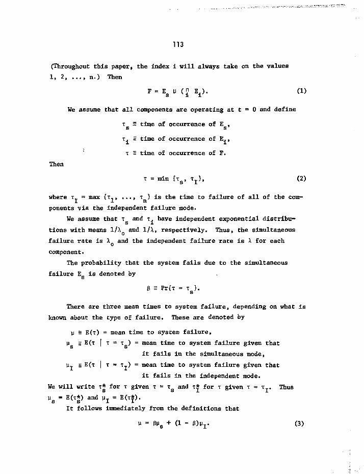
113

(Throughout this paper, the index i will always take on the values

1, 2 n.) Then

F = Eg U (" E ± ) . (1)

We assume that all components are operating at t = 0 and define

T 2 time of occurrence of E ,

x. = time of occurrence of E.,

T = time of occurrence of F.

Then

T = min {T S, T Z } , (2)

where T_ = max {x,, ,.., x } is the time to failure of all of the com-I X n

ponents -via the independent failure mode.

We assume that T and x. have independent exponential distribu-

tions with means 1/X and 1/X, respectively. Thus, the simultaneous

failure rate is A and the independent failure rate is A for each

component.

The probability that the system fails due to the simultaneous

failure Eo is denoted bys

6 = Pr{x = T }.s

There are three mean times to system failure, depending on what is

known about the type of failure. These are denoted by

u = E(x) = mean time to system failure,

U = E ( x | x = x ) = mean time to system failure given thats s

it fails in the simultaneous mode,

Vj =E(x | T »• T_) = mean time to system failure given that

it fails in the independent mode.

We will write x* for x given x = x and x* for x given x = xT. Thus

u = E(x*) and u = E(x*).S S X X

It follows immediately from the definitions thatU = Bus + (1 - 3)u r (3)

114

3. GENERAL RELATION BETWEEN 0 AND u

Theorem 1. Consider a system which can fail in a simultaneous mode or

in one or more competing modes. If the time to a simultaneous failure

is statistically independent of the times to failure of the competing

modes and is exponentially distributed with mean 1/X , then

8 - XQV . (4)

Remarks.

(i) This theorem treats a more general system than this paper con-

siders. Note that the statement of the theorem assumes nothing about

the distributions of the times to failure for the competing modes. The

theorem requires only that the simultaneous failure time be exponen-

tially distributed and be independent of the times to failure of any

competing failure modes. There is no restriction on the nature of

these competing failure modes. In particular, it is not required that

the components fail independently,

(ii) Note that (4) implies that AQy <_ 1. This is known to be true

since I/A is the mean time to failure for the simultaneous mode ando

must be larger than y, the mean time to system failure,

(iii) A heuristic argument for (4) is as follows. Start the system at

time t = 0 with all components operating. After each system failure,

reset the system by replacing all failed components and let the system

run, starting from the time of the previous failure. For any time

period of length T, letm(T) = number of system failures,

m (T) H number of simultaneous failures,s

Then, for large T,^ (T)

The assumption that the simultaneous failure times are exponen-

tially distributed implies that the simultaneous failure process is

without memory, that is, the probability of occurrence of a simulta-

neous failure at any time point does not depend on the previous history

115

of the process. Thus, the times of occurrence of the m (T) simulta-s

neous failures are independent of the times of occurrence of all pre-

vious system failures and competing failure modes and have the same

distribution as m *(T), the number of simultaneous system failures ins

a system subject only to simultaneous failures. But, for large T, the

number of system failures is approximately T/p. Thus

and

m(T) ~ 1

m (T) «= TXs o

Substituting these expressions into (5) and letting T -»• » then yields

(4).

(iv) The following result is needed for the proof of the theorem.

Lemma. Let X be a nonnegative random variable with cumulative distri-

bution function G(x). If E(X) exists, then

E(X) - £ " [ i _ G(x)] dx . (6)

Proof. By integration by parts,

E(X) - | % dG(x)

- - f x d[l - G(x)]

= /°° [1 - G(x)] dx - lim x[l - G(x)] .0

To evaluate the limit, note that

x[l - G(x)] ix°° u dG(u) ,

which approaches 0 as x -*- °°, since E(X) exists. Thus the limit is 0

and (6) holds.

Proof of Theorem 1.

Ve use the same notation as in Sect. 2, except that the subscript

I now refers to the failure of the system by any mode other than the

simultaneous mode. Denote the cumulative distribution functions (cdf)

of T , T_, and T by G , G , and G, respectively,Si Si.

The system reliability function is defined by

116

R(t) = Pr{system survives to t}

= Pr{x >_ t}

- 1 - G(t) . (7)

Then, from (2),

R(t) = Pr{x > t, T T > t}S J.

[1 - GCt)][l - G_(t)] . (8)S J_

Since E(x) <_ 1/X , we can apply the Lemma to (8) to get

y = E(T) = f R(t) dt

= f ll ~ G8<t)1[1 " G I ( t ) ] dt

By definition*,

0 = Pr{x <_ T }

* f Pr{xT > t | x = t} dG (t)o I — ' s s

= /°° [1 - G (t)] dG (t)0 I S dG (t)

But, since G (t) = 1 - e~Aot, application of (9) to (10) yieldssg = A V" This completes the proof.

4. FIRST AND SECOND MOMENTS TO THE TIMES OF FAILURE

For the system under consideration, the cdf of x iss

and the cdf of x is

G (t) = 1 - e " ^ , (11)s

x j xn < t}

= (1 - e " U ) n . (12)

From (8), the system reliability function is

R(t) - e"Aot[i - (1 - e"Xt)n] . (13)

*This part of the proof is due to W. A. Thompson, Jr.

117

Using (9), making the change of variable x » e~ ot and writing

S = X/X , we have

„ = i - f e"V(1 . e-V)» dt

= r - t f <* - x°>"dx0 0

" f " f i 1 Jo felt-"" ^0 0

"X~ " ITkpoU^"1' k6 + 1O 0

n /n\ t+i i

This can be expressed as a product as follows. Define

Xoa = T ,

and note that

1 .1 k + a - 1 ,

kT^;-1 y dy-

Substituting into (14), we have

1 n /n\, ,.k+l 1

x 6 y

1 ,1 o-lr. .. .ni

U - (i - y) ]1 1 .1 a-l,.

— ~ x i y a -

118

But the integral is equal to the beta function

B(a' n + 1} - r(a + n + 1)

r(a)nl

and hence

r(o + l)jL(a +k)

a k=l a + k

1 r. « kX I n -v

" = H 1 " k2i ITTkx J • <15)

It follows immediately from (4), (14), and (15) that

vk+l xoA©'-"1k = l W v "' A + kXo

~ J i xTT

By definition,

U = E ( T | T = T ) = / t dG*(t). (17)S S O S

From (9), (11), and (12),

6G*(t) = G (t) - /' G (x) dG (x)S o V A. o

« i - e"Xot - /fc X e~X°x[l - e~ X xl n dx . (18)

o o L J

Substituting (18) into (17), expanding as in (14), and noting that

V = 3/X , we have

119

An expression for y_ can be obtained by a similar argument or by

substituting (14) and (19) into (3). We get

u 1 g fn\r k+1 kX

Using a different approach*, it is possible to get a simpler

expression for JJ . Prom (16),

- 6) = J^ ln(kX) - J x ln(XQ + kX) .

Differentiating this with respect to X then yields

*p n i

O 0

Now differentiate (4) with respect to X to get

(22)-"o " °"o

But from (14) and (19),

Substituting (22) and (23) into (21), we get

V - X^W_ n i

1 - 6 k=l XQ + kX *

But, from (4) and (3), the left-hand side of (24) is equal to u •

Hence

f+kX ' (25)

^Suggested by V. R. Uppuluri.

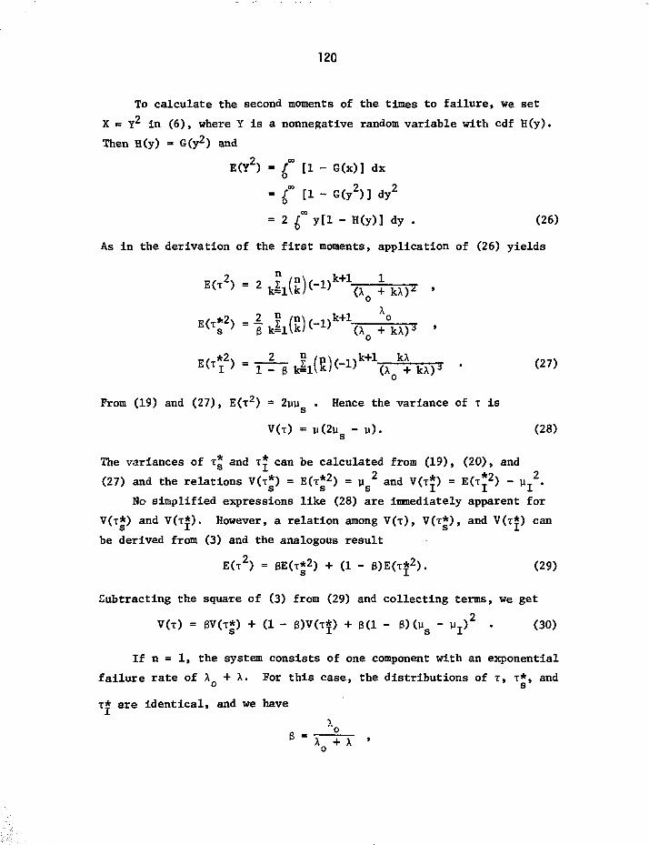
120

To calculate the second moments of the times to failure, we set

X = Y2 in (6), where Y is a nonnegative random variable with cdf H(y).

Then H(y) - G(y2) and

E(Y2) - £ [1- G(x)] dx

= £ [1 - G(y2)] dy2

= 2 £ y[l - H(y)] dy . (26)

As in the derivation of the first moments, application of (26) yields

0

From (19) and (27), E(T 2) = 2yu . Hence the variance of T iss

V(T) = y(2u - u). (28)s

The variances of x* and x* can be calculated from (19), (20), and

(27) and the relations V(T*) = E(x*2) = u 2 and V(x*) = E(x*2) - uT2.

S S S X X -L

No simplified expressions like (28) are immediately apparent for

V(x*) and V(x*). However, a relation among V(x), V(x*), and V(x*) canS i S J.

be derived from (3) and the analogous resultE(x2) = BE(x*2) + (1 - g)E(x*2). (29)

S J.

Subtracting the square of (3) from (29) and collecting terms, we get

V(x) = 3V(x*) + (1 - 6)V(x*) + 6(1 - B)(u - y T )2 . (30)

If n = 1, the system consists of one component with an exponential

failure rate of A + X. For this case, the distributions of x, T*, and

T* are identical, and we have

121

V(T) = V(T*) + V(T*) = (x \ x)2 • (31)

For the case n = 2, (4), (14), (19), (20), and (28) reduce to

X (X + 3X )

° °<*o

<*o

+ X)

X +0

+ X)

X20

<Xo

3X

<V+ 6X

+ 2X) '

+ 2X) »

oX + 7X2

s (X + X)(X + 2X)(X + 3X) '0 0 0

2X + 3XoJI (Xo + X)(X Q + 2X) '

V<T> = (X + 2 X ) ^ • <32>o

5. INEQUALITIES ON THE MEAN TIMES TO FAILURE

We will now prove that, for n > 1, the mean time to a simultaneous

failure is always less than the mean time to an independent failure,

this is, v < ]iT. In view of (3), this is equivalent toS X

Vg < v < vT , n > 1 . (33)

(i) This result holds for all values of X and X and exhibits the

effect of conditioning on the type of failure. For example, suppose

X « X so that $ = 0. Then \i =s y « 1/X , the mean time to a

simultaneous failure independent of a system failure. However, for the

system to fail due to a simultaneous failure, the simultaneous failure

must occur before an independent failure, and this can happen only if

the waiting time to the simultaneous failure is much less than its

122

mean I/A . In fact, by (33), the mean time y is less than y.o s(ii) Because the variance of T is positive, it follows from (28) that

2y is greater than y. Thus,s

y < y < 2y . (34)s s

(iii) In view of (3), (33) is equivalent to y < y . Hence it iss

sufficient to prove the following theorem.

Theorem 2. For all n < 1, and all A , A > 0,V < U . (35)

Proof. Consider y as a function of A . From (23),

8A \y/ MZ 3A "* yo o

9 /I \Therefore, proving(34) is equivalent to showing that .. I —1 < 1.°

A n(A + kA)From (15), °

IkA) - H(kA) '

where the product is taken over k = 1 n. We can now write

n(A + kA) = A Q(A ) + n! An ,

where Q(A ) is an (n - 1) - degree polynomial in A with positive

coefficients. Thus (37) becomes

V ~ o + Q(A0) * (38)

But Q(A ) is an increasing function of A^ so that -r^— > 0. Differen-0 O OAQ

tiating (38) with respect to A and using (36), we have

s . n! An !^V. .U TOT)- 8Ao < '

This completes the ;roof.

123

6. BEHAVIOR OF 3

We study the behavior of 3, the probability of a simultaneous

failure, as a function of n. We write (4) as

and define

pl MlA ±

where &n = -—r—r- and vi = -r—r—r- from (31). Clearly, p n is an" A T A •*• A T A

increasing function of n. To see how fast it is increasing, we will

derive an inequality for pn . Note that pn is a function of X and X

only through a = Ao/X .

To get a lower bound for pn , note that, for n > 1,

n (1 + |) > 1 + aa , (41)

where

n 1an " k=l k *

From (16) and (41),

Pn= —n n

+ 1a

1 \

_ __J: \1 + aan/

To get an upper bound for pn, from (40) we have p < — = 1 + —

Combining, for n > 1 we have

124

It is well known that a n « In n for large n. Hence, from (43),

ft 1 § A / j * v

"n + l+~a8 a-*-* . (44)11 QJ

This result is not surprising since, intuitively, ^n + 1 as n + » .

7. CGMPONENT VS. SYSTEM FAILURES

For any specific component, define

6 B probability that the component fails

by the simultaneous mode,

V = mean time to component failure.

Since focusing on a specific component is equivalent to the case

n • 1, we have from (31) that

*-T4T ,

1

From (35),

i-5-fipn

Since pn > 1 for n > 1, (46) expresses the unsurprising result that the

probability of a simultaneous failure and the mean time to failure are

larger for the system than for any specific component.

If n = 2, from (32),

o = r = ! ~ i—rrr • (*7)

Hence for all Ao, X > 0,

4 < f~ , £- < 1 • (48)

125

REFERENCES

1. A. W. Marshall and I. Olkin, "A Multivariate Exponential Distribu-

tion," Journal of the American Statistical Association, 62(1967),

30-44.

2. K. N. Fleming et al, HTGR Accident Initiation and Progression

Analysis Status Report, GA-A13617, Vol. II, General Atomic, 1975.

3. B. B. Chu and D. P. Gaver, "Stochastic Models for Repairable

Redundant Systems Susceptible to Common Mode Failures," in

Nuclear Systems Reliability Engineering and Risk Assessment,

J. B. Fussell and G. R. Burdick, eds., Society for Industrial

and Applied Mathematics, 1977.

4. Frank Proschan and Pasquale Sullo, "Estimating the Parameters

of a Multivariate Exponential Distribution," Journal of the

American Statistical Association, 71(1976), 465-472.

THE USE OF SEMI-CONTROLLED EXPERIMENTS IN

THE ANALYSIS OF RESIDENTIAL ENERGY DEMAND

Lawrence S. Mayer-Department of Statistics

Princeton University

ABSTRACT

The experiences of statisticians on theTwin Rivers energy research program are reviewed.The general advantages of using experimental pro-grams in research on residential energy usage areconsidered along with the limitations of competinganalytic approaches. It is argued that researchin this area and other policy relevant energyareas would benefit greatly from wider funding oflarge-scale experimental programs and that statis-ticians could play a key role in the design, exe-cution and analysis of the experiments. Reasonsfor the rarity of large-scale statistical experi-mental research programs which analyze residentialenergy demand are considered. The major rolesthat statisticians played on the Twin Rivers pro-gram are discussed and some of the results obtained,in part, by the statisticians on the project arereviewed.

The research reported in this paper was supported,in part, by the Department of Energy under ContractNo. EC 77-S02-4288, awarded to Princeton University.This report was prepared, in part, through thesupport of the Energy Information Administration.

126

127

1. INTRODUCTION

Recent events have significantly increased the interest

of academics and policy makers in the "Twin Rivers" Energy

Research Program. The program, which began in 1972 and ended

in 1978, contributed to our understanding of the residential

energy environment through six years of experimental studies

of a single planned residential community, Twin Rivers,

New Jersey. These studies focused on analyzing the variation

in energy utilization across similar housing units, across

time, across fuels and across families. Although numerous

articles have been produced by the project, no discussion of

the experiences relevant to energy statisticians has appeared.

As the principal investigator charged with supervising the

design, collection, storage, management, and analysis of the

large data sets generated by the project, I will proffer such

a discussion. Furthermore, I will use the review as a vehicle

to comment on the potential role of experimental programs and

the statistician in residential energy research and research

in related areas.

Interest in the Twin Rivers project has increased sharp-

ly for a variety of reasons. First, the visibility of the

project has been increased by the recent appearance of publi-

cations containing the results of experiments which took sev-

eral years to complete. In fact, one energy journal has de-

voted an entire issue to output of the project, and a related

book which presents some of our results recently appeared.

Second, the project, which began under the auspices of the

National Science Foundation, has become atypical of energy

research programs since the Department of Energy has chosen

not to sponsor a large number of multi-year, large-scale,

interdisciplinary, experimental field studies of the consump-

tion and conservation dimensions of the residential (or any

other) energy sector. Finally, the National Energy Flan pro-

posed by President Carter and the National Energy Act pro-

duced by Congress both include provisions for reducing our

128

total energy demand by encouraging conservation in the resi-

dential sector. These provisions have increased the desire

of policy makers and private sector decision makers to under-

stand the dynamics and the potential for energy conservation

of the American home. The Twin Rivers project has yielded

important contributions to that understanding.

In order to understand the statisticians' role on the

Twin Rivers project, it seems critical to distinguish between

policy analysis and policy relevant research. Policy analysis

is research undertaken to analyze or to promote a particular

policy decision and possibly should be called "advocacy re-

search." For example, a study designed to show, assess, or

increase the political wisdom of the nation making a signi-

ficant investment in the development of "soft" energy tech-

nologies is policy analysis. Policy relevant research is

research which is scientific in nature but which addresses

issues which have direct bearing on the policy process. For

example, research which tests the field performance of com-

peting building materials is policy relevant research.

I am concerned with examining the use of experimental

programs in policy relevant research on the residential en-

ergy environment. I suggest that statistical experimental

methods are underutilized in this type of energy research

and that if such methods were utilized to their full poten-

tial, then the statisticians1 role in energy research would

become highly significant.

The Twin Rivers program is an excellent example of

policy relevant research. As evidence, the project investi-

gated the potential of reducing residential energy demand

by physically modifying the structure of the dwelling. This

investigation produced statistical information which is

directly relevant to the political decision of whether to

try to reduce our residential energy demand by adopting more

energy efficient building standards. The study focused on

129

the direct effects on demand and direct economic consequences

of the modifications and not on the associated policy ques-

tions, and thus is not policy analysis. The distinction be-

tween policy analysis and policy relevant research may be

critical for our profession (energy statisticians), since

the Energy Information Administration (EIA) may become a

major conduit through which statisticians are involved in

energy research, and it is forbidden, in its enabling legis-

lation, from being involved in policy analysis. On the

other hand, the EIA is directly charged with producing infor-

mation which is critical to the formulation and execution

of sound public energy decisions.

I suggest, but do not have space to complete a formal

argument, that statisticians, by virtue of their training,

experiences, and rather unique perspective on interactions

among factors in the world, are particularly suited to play

a major role in policy relevant energy research, but, in

fact, are playing the most minor of parts. Much of the

energy research which has been produced since the Arab oil

embargo would, in my opinion, have benefitted significantly

by increased use of systematic experimental methods; by

coordinating such studies the statisticians would make a

major contribution to scientific research which is relevant

to energy policy.

With regard to several parameters the Twin Rivers pro-

ject was probably typical of successful large-scale empirical

policy relevant research programs. It was a collaborative

program involving several disciplines across several colleges;

it relied on large longitudinal experiments to gather its

data; it addressed issues of immediate concern to policy

makers; it generated huge amounts of data, only a small frac-

tion of which will ever be systematically examined; it was

able to capitalize on a good deal of associated physical

theory but worked on problems for which there is no compre-

130

hensive theory; and it worked in an area in which classical

wisdom often proves to be inadequate for current policy de-

cisions. I suggest that the explicit and implicit roles of

the statisticians in this program are probably typical of

the roles on similar large-scale policy relevant experimental

programs.

Twin Rivers, itself, is a single planned community 30

miles from New York City which consists of garden apartments,

owner-occupied townhouses, single family detached houses, and

commercial establishments. The project designed, developed,

managed, and analyzed a variety of data sets. These sets

differ with regard to the number and choice of housing units

monitored, and the level of detail and frequency of the

measurements made on each unit. Each data set was designed,

in the statistical sense, to some degree. One set includes

the design characteristics, demographic variables, and month-

ly energy demand statistics for 401 two-story townhouses

and 151 split-level townhouses. A second set includes 67

variables monitored every 15 minutes for four units, variables

related to the end use of energy in the unit (room tempera-

tures, door and window openings, attic temperature, appliance

usage, etc.). These measurements were relayed over telephone

lines to our laboratory and recorded automatically on magnetic

tape. A third set contains engineering measurements obtained

from a leased townhouse which was examined in minute detail

by our engineers. A fourth data set, which is possibly the

most interesting in terms of my theme, includes data on eight

key variables for 32 townhouses monitored once per hour and

recorded on cassettes by a small electronic device located

in the basement of each sample unit. These data are part of

an "Omnibus" experiment which will be discussed below.

In reviewing the experiences of statistician . on the

Twin Rivers project, I will address the following questions:

131

(i) In what Fsnse can projects such as the Twin Rivers

program, which use a statistical experimental approach,

contribute to energy information? Why is an experiment-

al approach preferable to competing approaches for

understanding the residential energy environment?

(ii) If large-scale statistical experimental field programs

can make important contributions to information about

the residential and other energy environments, and thus

to energy policy, why aren't there more of them?

(iii) In what sense can statisticians contribute to such pro-

grams? Are there examples of knowledge that were

gained by the Twin Rivers project that may not have

been gained if it were not for the heavy involvement

of statisticians?

2. RESIDENTIAL ENERGY EXPERIMENTS:

THEIR IMPORTANCE AND THEIR RARENESS

Large-scale statistical research programs that rely as

much as possible on designed experimental frameworks have

the potential to make a strong contribution to our understand-

ing of residential energy consumption. In spite of this po-

tential, such programs are few in number when compared to

other types of programs such as laboratory experimental pro-

grams, product development and design efforts, computer simu-

lations, and statistical modelling efforts which rely on

secondary data generated for purposes other than statistical

analyses. Furthermore, the existence of this potential implies

that statisticians could have major involvement in energy re-

search by virtue of their ability to contribute to experimental

programs. In part, to encourage the funding of more experi-

mental programs and the involvement of more statisticians is

to delineate the contribution that both could make.

In the study of the residential energy environment four

difficult and critical problems, in my estimation, are best

approached by experimental methods. The first two are to

132

estimate the actual (as opposed to theoretical or simulated)

size (and variation) of the effects of various factors on the

utilization of energy in the residential unit and to estimate

the size of the interactions associated with these effects.

Factors include physical parameters such as the size and de-

sign of the unit, quality of construction, the amount and type

of insulation, and the local weather conditions; economic fac-

tors such as the stock of appliances, local energy prices,

and family income; and social psychological factors such as

family size, the utilization of the unit, the level of know-

ledge of conservation measures and the attitudes of the resi-

dents towards energy conservation.

The last two problems are to estimate the effect that

changes in one or more of these factors have on the other fac-

tors, and to estimate the effect that changes in one or more

factors will have on residential energy usage. These prob-

lems are relevant to public policy since public policies can

be used to encourage changes in dwelling design, construction

materials, construction quality, appliance efficiency, as

well as changes in energy prices, the utilization of the home,

the amount and quality of energy information available to

residents, and in many other factors. The degree to which

changes in any one of these factors affect the other factors

is a policy relevant topic for experimental research. For

example, architects and builders could be encouraged to adopt

new designs for residential buildings. The degree to which

such designs would affect the behavior of the occupants can

be studied by experimental methods. Similarly, the degree

to which such design modifications would affect residential

energy usage is a topic for experimental research.

I suggest that these four problems can be studied by

experimental programs and further contend that they cannot

be analyzed effectively unless experimental design and analy-

sis principles are used, since the response of primary

133

Interest, energy usage, Is affected by dozens of factors of

various types. The effect of a factor on demand, the asso-

ciated interactions, the effect that changes In factors have

on other factors, and the effect changes In factors have on

energy usage can be estimated accurately only by experiments

in which some "competing" factors are controlled by design

or selection and other competing factors are controlled by

statistical methods. Otherwise, it is impossible to choose

among competing explanations of the statistical variations

in demand across units, across time, and across fuels. In

fact, of the dozens of physical, economic, sociological, and

behavioral factors that affect residential demand, it is pro-

bably true that almost any two significant factors are corre-

lated across randomly chosen units. Furthermore, the major

factors probably interact in their effects on energy usage.

It is absolutely impossible to unravel these interactions

without the use of an experimental approach. Finally, those

factors which are extremely important in developing energy

policy are often factors,such as price or amount of insula-

tion, which have minor effects on residential energy demand

when compared to factors (e.g., weather) which are beyond

policy considerations. Therefore, it is important to formu-

late analyses which control, by design, selection, or statis-

tics, for factors which confound, mask, or overwhelm the

effects of factors relevant for policy.

Having argued that application of the principles of sta-

tistical experimental design is critical if studies of resi-

dential energy demand are to help in providing the knowledge

needed to develop sound energy policy, it is important to

warn statisticians that it is almost impossible to conduct

an optimally designed experiment in the residential energy

area. The prohibitive constraints are straightforward and

are similar to constraints on using designed experiments in

other areas of energy research. First, several factors which

134

are key determinants of energy demand can only be controlled

by restricted sample selection. Second, several key factors

can be neither controlled nor eliminated from the design.

Third, several key factors are almost impossible to measure.

As examples, the solar load on the dwelling can be controlled

only by analyzing units in a single region; appliance config-

uration probably can neither be controlled nor eliminated by

sample selection; and, finally, the quality of construction

of the dwelling and the behavior of the occupants are almost

impossible to measure and thus impossible to control. The

variation due to these factors cannot be assigned to the

"error" category since these factors vary systematically over

units and may be highly correlated with factors which are

controlled by design, factors such as dwelling size, family

size, and the market value of the unit. Schemes which alter

the quality of the original construction or which would mod-

ify the behavior of the occupants, perhaps by forcing occu-

pants to refrain from certain behaviors, may be possible but

are probably neither practical nor ethical. Finally, actions

of the occupants may make it impossible to assign or keep

certain units in a treatment group. For example, occupants

might force the experimenter to remove insulation added to

the furnace ducts if the occupants have decided to finish

their basement.

Since it is desirable to control for as many of the fac-

tors affecting residential energy utilization as possible,

but it is probably impossible to control for as many factors

as would be necessary to deem the experiment "designed," the

experiment might be labeled "semi-controlled" or "semi-

designed." Such experiments can be summarized by the follow-

ing characteristics:

(i) To whatever extent practical, the principles of experi-

mental design are used to develop the primary data

gathering mechanisms. Major factors of energy demand

135

are experimentally controlled whenever possible.

(ii) The responses of Interest are affected by many factors,

some of which (e.g., occupant behavior) cannot be con-

trolled experimentally, statistically, or by sample

selection.

(ill) The factors that are experimentally controlled inter-

act with the factors which are not controlled, and

there is no way to estimate these interactions.

(iv) The factors used to define the design are thought to

contribute much less to the variation of the response

than factors which cannot be measured and thus cannot

be controlled (e.g., quality of construction),

(v) Often a sample unit cannot be assigned to the optimal

treatment group due to physical or consent limitations.

(vi) At least one major covariate (e.g., weather) must be

dealt with statistically.

The strategy in designing a semi-controlled experiment

is usually to use a restricted sampling frame which slices

the population of interest and thus physically controls for

many of the factors which cannot be incorporated into the ex-

perimental plan. Within this sampling frame units are assigned

to treatment groups as optimally as possible without violating

physical, legal, or consent constraints. Statistical infer-

ences are limited to the restricted population.

Most of the studies conducted as part of the Twin Rivers

program involved semi-controlled experiments. As one example,

the "Omnibus" experiment used a partially (and approximately)

balanced incomplete longitudinal design to test the effects

of three physical retrofit packages on energy demand profiles

of the residential unit. Eight variables, including total

energy demand, natural gas demand for the furnace, thermostat

settings, door and window openings, and temperatures at the

various rooms, were recorded hourly. The sample units were

chosen from the population of interior two-story townhouses

136

in one section, Quad II, of Twin Rivers. By using this samp-

ling frame numerous sources of variation that would be found

in an experiment involving a random sample of American housing

were eliminated. The units are only of three sizes, of ex-

actly the same design, built by a single builder, and equipped

with almost identical appliance configurations. The occupants

tend to be married, young, middle-class natives of the New

York region with one or two children. Family income is fairly

constant over the sample. Almost all of the children attend

a single school. Although the physical location of the units

varies, all of the units are in one small neighborhood and

thus face similar wind and solar conditions. The two major

factors that could not be controlled in the "Omnibus" experi-

ment are the quality of construction and the behavior of the

occupants. Among the factors which were controlled by assign-

ing the sample units to treatment groups are the size, prior

level of demand, location of the unit in the neighborhood,

and the compass orientation of the unit. The experiment

showed that the retrofit packages significantly reduced the

overall demand for energy, and of equal importance, signifi-

cantly redistributed the flow of energy through the residen-

tial unit. A valid demonstration of these effects probably

would have been impossible without the use of statistical

controls because the effects of the "treatments" on consump-

tion are small when compared to the effects of factors that

were controlled by restricting the sampling frame and by

balancing the design.

Having suggested that research programs which utilize

semi-controlled experimental methods can make a major contri-

bution to our understanding of the residential energy environ-

ment, it becomes imperative to speculate on the reason that

the number of such projects in the energy area is so small

when compared to the number in other research areas such as

health care delivery. Along this line, it is interesting to

137

note that the Twin Rivers project was originally sponsored by

the National Science Foundation and was inherited by the Energy

Research and Development Administration when the National

Science Foundation was ushered out of funding energy research.

It has never been clear that ERDA or its descendants would

have initiated the funding. The statistical experimental na-

ture of the program has never been embraced as warmly by the

energy agencies as it was by NSF.

The major impediment to the initiation of statistically

oriented, large-scale, policy relevant experimental programs

which focus on the residential energy sector is the existence

of divaricating perceptions of the residential energy environ-

ment. These perceptions arise, primarily, from academic divi-

sions of inquiry and from divisions among professionals in-

volved in the design, development, construction, sales, and

upkeep of residential units. Complex empirical studies that

emphasize the interactions among factors that fall in differ-

ent intellectual or professional arenas and emphasize concepts

such as assignment of units to treatment groups and tests of

hypotheses are not congruent with any single perception. It

is my experience that many developers, architects, builders

and engineers tend to view the residential unit as a physical

laboratory and view human factors and variation in construc-

tion to be nuisance factors that must be ignored or treated

as random error. Conversely, many economists, sociologists,

anthropologists, and psychologists tend to view the residen-

tial unit as a human environment and pay little attention to

the physical structure of the unit. The first approach ig-

nores the fact that all energy in the home is processed in

response to human action (setting the thermostat, doing the

dishes, etc.), and the second perception ignores the fact

that only physical processes can "use" energy. Both percep-

tions are antithetical to the reality that effective policies

for the residential sector must be policies which take into

138

account both the physical and the human determinants of energy

consumption, and, furthermore, must be sensitive to the subtle

interactions which exist between human behavior and physical

processes. Policy makers must be aware that most changes in

the physical environment alter the living arrangement and that

occupants may respond to the altered environment by modifying

their use of the dwelling. This modified behavior might in-

crease or decrease the effects of the physical changes on the

demand for energy and distribution of energy in the dwelling.

For example, adding attic insulation might reduce the differ-

ence between the upstairs and downstairs temperature in the

winter. The occupants may respond by reducing the thermostat

setting at night since it requires less fuel to be warm in the

upstairs. On the other hand, installation of an automatic

night thermostat set-back device might produce an uncomfort-

ably cold kitchen in the morning. The occupants might respond

to the device by increasing their use of the oven in the morn-

ing, a response which might cancel the direct effects of the

set-back device and actually increase overall demand.

The experimental approach is optimal only if one takes

the broadest, and most scientific, approach to studying the

residential energy environment and tries to unravel the entire

range of factors which affect residential energy usage. If

the goal of a study is to estimate the effect of a single

factor, be it a design factor, a weather factor, or a human

factor, on a component of energy demand, and if the inter-

action between that factor and the other factors is ignored

(a possibly fatal error), then often a study can be conducted

which provides some estimate and is far simpler and cheaper

than a large-scale experimental study. Unfortunately, the

lessons learned from such studies may be quite meager in that

the difficulty in making energy policy for the residential

sector is to assess the relative merits of complex, competing

policies and the interactions between the policies. Surely,

139

if the government legislated ten programs, each of which has

been shown to be capable of producing a five percent reduction

in residential energy demand, then no one would expect a fifty

percent reduction in demand; but what should be expected?

The overall effect of multiple policies cannot be estimated

unless the component policies are tested in conjunction with

each other and the interactions among the components are esti-

mated. In the limit, I am sure that it would be possible to

design a living environment which is incredibly physically

efficient but is so humanly intolerable that it requires the

occupants to consume a tremendous amount of energy in order to

survive. The experimental approach can not only transcend

traditional professions and disciplines, but it can combine

the wisdom from each in order to test the effects of various

energy policies.

It is interesting to note that most of the offices of

the Department of Energy can be identified with energy pro-

fessions and/or academic disciplines. It is not clear that it

would be rational for such offices to transcend boundaries

and invest their limited resources in large-scale, inter-

disciplinary experimental studies. To no one's surprise,

engineers are interested in engineering and sociologists are

interested in sociology. The energy statistician alone is

interested in sorting out the complex effects of multiple in-

terrelated factors on energy utilization. What are needed

are experimental studies of the residential environment in

which engineers lead the study of the engineering features of

the residential unit, sociologists lead the study of the socio-

logical aspects of the residential unit, and the statisticians

incorporate all of this expertise into experiments designed to

assess the effects of engineering and sociological factors,

among others, on demand.

140

3. THE STATISTICIAN'S CONTRIBUTION TOAN EXPERIMENTAL RESEARCH PROGRAM

It may be needless to tell those statisticians who work

with large experimental data sets (and it may be pointless to

tell others) that the most significant contributions that the

statistician offers a large-scale, policy relevant experimental

program do not involve the explicit application of statistical

theory. They do involve, however, the repeated application

of basic statistical principles, principles which are learned,

in part, in the classroom, and, in part, by working with data

in an experimental setting. Before reviewing what I believe

to be the most significant roles through which we, as statis-

ticians, affected the Twin Rivers program, I want to emphasize

that a tremendous learning process existed for the entire dura-

tion of the project. While we were learning about the physics,

engineering, economics, psychology, and architecture of the

residential unit, we were teaching the physicists, engineers,

social scientists, and architects about the process of using

data to systematically and fairly test theories and models

and the process of developing theories by both formal and

informal examination of data.

Probably the most important contribution the statisti-

cians made to the project was in displaying constant vigilance

in injecting, to whatever degree possible, basic principles

of experimental design in each and every data collection

effort. Although constraints prohibited the use of totally

designed experiments, statisticians insured that each completed

analysis had the maximum validity and the maximum impact, by

insuring that principles such as confounding, nesting, repli-

cations, covariates, and control groups were considered in

the design of each data set and the design of each analysis.

Resistance to strategies such as taking measurements on sample

units before introducing experimental treatments was slowly

overcome, as was resistance to monitoring unperturbed control

141

sample units. There is some tendency in an area where all of

the principles of experimental design do not apply not to use

any of the principles. Statisticians reminded the project of

simple statistical facts, e.g., that control groups were

needed* or that nested factors could not be isolated. This

vigilance saved our program from initiating experiments which

were impotent with regard to the issues for which they were

designed.

Secondly, the statisticians helped their colleagues learn

to analyze the variety of types of uncertainty present in al-

most all energy data. The idea that one can learn from statis-

tical analysis of patterns and trends in error-ridden data was

often foreign to the engineer and physicist. The statistician

constantly noted and estimated the various types of error that

"contaminated" each experiment and examined whether a data

set was too error-ridden to be useful in addressing the prob-

lems for which it was developed.

Third, the statisticians formally tested hypotheses.

Often, the engineers and physicists would become excited that

a particular portion of the data, for example, data for a

single day, was supporting one of their conjectures. They

did not systematically scrutinize whether, in fact, all of the

data were supportive. The statisticians were charged with de-

signing and executing formal statistical tests. It is in

this role that the statisticians were able to utilize statis-

tical theory and flex their mathematical muscles. It is the

role which most often leads to statistical research, publica-

tions, theses, and professional rewards from fellow statisti-

cians. Perhaps unfortunately, it tends to be a rather minor

role on experimental programs of the type being reviewed.

Usually the time constraints associated with policy relevant

research will not allow the statistician to pursue interesting

methodological problems unless he (or she) cloisters himself

off from the mainstream of the project. Such isolation may

142

produce better statistical results and may be consistent with

current academic fashion but tends to make the statistician

sacrifice roles which are critical for the program. The

statistician, by virtue of his (or her) understanding of the

vagaries of data, of the difficulty of designing an experiment

that addresses the issues of importance, of the different

types of error that plague the fitting of any model to field

data, and of the general process of learning from data, must

accept an ethical and practical commitment not to hide in a

back office doing research. He (or she) cannot forfeit the

responsibility of making sure that the conclusions reached by

the project are reached through application of the best avail-

able analytic techniques and that all published conclusions

are supported by data.

Fourth, the statisticians helped the project uncover

trends and patterns in the data and thus helped the project

develop models from data. Often in a project of the type be-

ing described here there is a tendency to bring models to

data in order to support, or, less often, to reject, the model.

Statisticians were instrumental in showing how to develop

models from the experience of exploring data.

Finally, statisticians spent a good deal of time criti-

cizing the data analytic efforts of those members of the pro-

ject not familiar with the subtleties of statistical method-

ology. One of the exasperations of being a statistician on a

large experimental project is that, although only engineers

are trusted to engineer, and only physicists have the license

to pontificate about physics, everyone has the freedom (and

encouragement) to analyze data. The statisticians played a

key role by keeping a watchful eye on the statistical efforts

of colleagues and their students. Exposing poorly done sta-

tistical analyses was a personally, though possibly not pro-

fessionally, rewarding task.

143

4. SPECIFIC TALES TOLD BY TWIN RIVERS

Host of the important lessons learned through the Twin

Rivers program were learned by the analysis of one or more of

the large data sets generated by the experimental projects.

Many of these lessons would not have been as focused or precise

and might not have been lessons at all were it not for the

heavy involvement of statisticians. Here are a few examples:

Statisticians led the study of the variation in monthly

energy demand for 1,000 units across time, across units, and

across fuels. The results of this effort are many and include

the following:

(i) About 50% of the variation in energy demand across

dwellings can be attributed to structural factors such

as the number of bedrooms, the number of neighboring

units, and the compass orientation of the unit,

(ii) The residents responded to the onset of the Arab oil

embargo by significantly reducing their demand for

natural gas but did not reduce their demand for elec-

tricity.

(ill) The demand for natural gas has decreased slightly over

the last few years, possibly in response to increases

in price. The demand for electricity has not decreased

over the same period, although the distribution of

electricity demand over end-uses has altered.

Also, by analyzing monthly data, statisticians developed

a simple measure of the coldness of the month, labeled "modi-

fied degree days," which is preferable to the traditional

"degree days" measure as a predictor of the fuel demand to the

furnace in the winter. The modified measure, unlike the tra-

ditional measure, is a function of the distribution of temper-

ature over the day. The modified measure proved useful in

adjusting fuel demand for the effects of the coldness of a

month and thus, in most experiments, for controlling weather

as a covariate.

144

Statisticians led in the design and analysis of the

"Omnibus" experiment. They attempted to estimate the effects

of three physical retrofit packages on demand through a

before/after partially-balanced design. Direct comparisons

of before-treatment and after-treatment demand for the ex-

perimental units were misleading since the units in the con-

trol group reduced their demand over the treatment period.

Using the before-treatment information, the before/after

comparison for the control group, and the values of the major

covariate, degree days, the after-treatment values of the

experimental groups were adjusted. These adjusted values

were used to show that the retrofits significantly reduced

the demand for natural gas for the experimental units.

Statisticians aided in the design and analysis of various

experiments conducted by social psychologists. These experi-

ments tested the effects of feedback to the occupants on their

demand for energy. Statisticians also aided in designing the

mechanisms of feedback used in the experiment. They included

mechanisms which indicated the ratio of the actual fuel de-

mand to the predicted demand using a simple, regression func-

tion of degree days. Statistical anlaysis showed that some,

but not all, of the feedback mechanisms significantly reduced

demand.

Finally, statisticians developed a simple one-person,

90-minute procedure for auditing the energy characteristics

of any residential unit, including a mobile home or a high-

rise apartment. This procedure was developed by distilling

the more thorough two-day audit developed by the project's

engineers. The audit design emphasizes the need for collect-

ing statistically useful information with minimal risk and

disruption. Hopefully, the audit will be useful in a nation-

al survey of the energy characteristics of American housing.

145

5. CONCLUSIONS

The Department of Energy should consider initiating the

funding of statistical experimental programs which analyze

the residential sector (and other sectors). Such programs

should use semi-controlled experiments to the extent possible

without surpressing the dynamic complex nature of the resi-

dential environment. These experiments could concentrate on

assessing the accuracy of physical, economic, and social

models of residential energy consumption; developing improved

models of residential energy usage; examining the complex

interactions among the design, construction, and physical

characteristics of the residential unit, the economic factors

of demand, the demographic characteristics of the "family,"

and the attitudes and knowledge of the occupants; developing

a reliable data base on the temporal and seasonal variation

in key energy variables for a variety of types of residential

structures in a variety of regions of the country.

We are learning too slowly about the dynamics of our

existing residential energy environment. Too much existing

"knowledge" about our environment was "developed" during

periods of low energy prices, growing demand, and virtually

no perception of a need to conserve fuels. It is not clear

that this knowledge is accurate enough, complete enough, or

has been challenged sufficiently to allow the various levels

of government to use it in making good decisions regarding

public energy policies. Optimal use of experimental methods

would radically increase our knowledge. The Twin Rivers

project was movement in the right direction but only a step.

IMPROVING THE RELIABILITY

OF ECONOMETRIC MODELS*

Roy E. Welsch

Massachusetts Institute of Technology

Cambridge, Massachusetts

ABSTRACT

This paper describes new techniques that can help to im-prove the reliability of econometric and other models. Diag-nostic methods are employed to discover influential observations— those which may have undue importance in determining predic-tions, coefficient estimates, etc.

Techniques based on the deletion of a single observationare the most developed and will be briefly summarized. Recentresults on the deletion or perturbation of subsets of obser-vations will be described in connection with the use of leverageplots. A new fitting procedure called bounded influence esti-mation is also discussed.

These methods will be applied to a model with thirteenexplanatory variables which tries to relate housing prices tolevels of pollution in 506 Boston Metrolpolitan Area censustracts.

*Supported in part by National Science Foundation Grant77-26902MCS to the M.I.T. Center for Computational Researchin Economics and Management Science.

146

147

1. INTRODUCTION

Economists and others have been building and using econometric models

for many years. A subset of these builders and users have always been con-

cerned about model reliability, sensitivity, and validity. The energy

crisis put certain aspects of modeling into the public and political spot-

light. Many questions have been raised about the integrity of the modeling

process and in 1975 the National Science Foundation sponsored a conference

at Vail, Colorado on model formulation, validation, and improvement [5 ].

This conference caused a number of statisticians to pay more attention to

the statistical questions raised in connection with model reliability, sen-

sitivity, and validity. This paper briefly describes some of the progress

that has been made by examining a particular model and set of data. What

follows should in no way be construed as a complete analysis of the data

or model.

We will denote the standard regression model by

y = X3 + e (1)

where X is n * p. The least-squares estimates for 3 will be called b,

the estimated residuals, e, and the standard error of the regression, s2.

The notation (i) will be used to indicate that the i row or observation

has been removed from a computation and x. will denote the i row of the

X matrix.

2. DATA AND MODEL

The data and model we will discuss are taken from a recent paper by

148

Harrison and Rubinfeld [3 ]. A two-step procedure is used by them in

order to estimate the willingness to pay for reduced air pollution. The

first step is the estimation of a hedonic housing price equation, and the

second step is the estimation of a marginal willingness to pay function

for households in an urban area. We will only examine the first step in

what follows.

The hedonic housing price model used by Harrison and Rubinfeld is

MV = gj + e2CRlME + g3ZONE

+ 3^INDUS + 65CHAS + 66NOXSQ

+ 37ROOM + 3sAGE + B9DIST (2)

+ gioHWAY + 611TAX + 0i2PTRATIO

+ 313BLACK + Bj4STATUS + e.

A brief description of each variable is given in Table 1. Further details

may be found in the Harrison and Rubinfeld paper.

Table 1

Definition of Model Variables

Variable Definition

MV Logarithm of the median value of owner-occupiedhomes.

CRIME Per capita crime rate by town.

ZONE Proportion of a town's residential land zonedfor lots greater than 25,000 square feet.

INDUS Proportion of non-retail business acres per town.

CHAS Charles River dummy variable with value 1 iftract bounds the Charles River.

NOXSQ Nitrogen oxide concentration (ppm) squared.

ROOM Average number of rooms squared.

AGE Proportion of owner units built prior to 1940.

DIST Logarithm of the weighted distances to five em-ployment centers in the Boston region.

149

Table 1 Cont.

Variable Definition

HWAY Logarithm of index of accessibility to radialhighways.

TAX Full value property tax rate (per $10,000).

PTRATIO Pupil-teacher ratio by town school district.

BLACK (B-0.63)2 where B is the black proportion ofthe population.

STATUS Logarithm of the proportion of the populationthat is lower status.

The basic data is from census tracts in the Boston Standard Metro-

politan Statistical Area (SMSA) in 1970. With tracts containing no housing

units or composed entirely of institutions excluded, the Boston sample

contains 506 observations. To aid in understanding the results which

follow, we provide a breakdown of the observations by town in Table 2.

In the process of developing the model (2), Harrison and Rubinfeld

were careful to reduce collinearity as much as possible. To check this

we computed the condition number (the square root of the ratio of the

largest and smallest eigenvalues) of the scaled explanatory variable matrix

and found it to be about 66, well within the range needed to ensure the

accuracy of their (and our) results. Harrison and Rubinfeld also discuss

possible heteroscedasticity, but eventually settle on the model (2) with

no heteroscedastic weighting.

In order to summarize the data, we present some of the standard out-

put from least-squares regression. Table 3 lists the estimated coeffi-

cients, standard errors, and t-statistics, along with F, R2, and s2.

150

Observation

12-34-67-1314-3536-3940-4142-5051-545556575859-646566-6768-7071-7475-8081-8485-8889-9293-9596-100101-111112-120121-127128-142143-172173-179180-187188-193194-195196197-199200-201202-203204-205206-216217-220221-238239-244245-254255-256257258-269270-274

Table 2

Census Tracts

Town

NahantSwampscottMarbleheadSalemLynnSaugusLynnfieldPeabodyDanversMiddletonTopsfieldHamiltonWenhamBeverlyManchesterNorth ReadingWilmingtonBurlingtonWoburnReadingWakefieldMelroseStonehamWinchesterMedfordMaidenEverettSomervilleCambridgeArlingtonBelmontLexingtonBedfordLincolnConcordSudburyWaylandWestonWalthamWatertownNewtonNatickFraminghamAshlandSherbornBrooklineDedham

Observation

275-279280-283284285286287288-290291-293294-298299-301302-304305-308309-320321-328329-331332-333334-341342343344-345346-347348349350-351352-353354355-356357-488

357-364365-370371-373374-375376-382383-393394-406407-414

415-433434-456457-467468-473474-480481-484484-488

489-493494-501502-506

Town

NeedhamWellesleyDoverMedfieldMillisNorfolkWalpoleWestwoodNorwoodSharonCantonMiltonQuincyBraintreeRandolphHolbrookWeymouthCohassetHullHinghamRocklandHanoverNorwellScituateMarshfieldDuxburyPembrokeBostonAllston-BrightonBack BayBeacon HillNorth EndCharlestownEast BostonSouth BostonDowntown (South

Bay)RoxburySavin HillDorchesterMattapanForest HillsWest RoxburyHyde Park

ChelseaRevereWinthrop

151

INTERCRIMEZONEINDUSCHASNOXSQROOMAGEDISTHWAYTAXPTRATIOBLACKSTATUS

Table 3

Regression Results

R2 = 0.81 s2 =

EST COEFF

9.756- 0.01190.00008040.0002420.0914

-63.8070.006330.0000897

- 0.1910.0957

- 0.00042- 0.03110.364

- 0.371

0.18 F(13

STD ERR

0.150.00120.00050.0020.033211.3150.001310.00050.0330.01910.000120.0050.1030.025

,492) =

T-STAT

65.23- 9.530.160.102.75

- 5.644.820.17

- 5.735.00

- 3.42- 6.213.53

-14.83

157

Many econometric texts and discussions of econometric models fail to

place enough emphasis on the verification of statistical assumptions. For

example, Harrison and Rubinfeld do not mention or display a Gaussian (nor-

mal) probability plot of the residuals. Figure 1 is a plot of the stu-

dentized residuals (these particular residuals are explained more fully

in Section 4) and we note the heavy tails perhaps indicating that the

Gaussian error assumption is suspect. The largest residual, 372, is de-

noted on the plot.

In general, we would also look at the residuals against each explana-

tory variable. It is more informative to make partial-regression plots.

This graphical device can be motivated as follows. Let X[k] be the

n x (p _i) matrix formed from the data matrix, X, by removing its k1" column,

X, . Further let u. and v. , respectively, be the residuals that result from

regressing y and X, on x[k]. As is wall known, the k regression coeffi-

cient of a multiple regression of y on X can be determined from the simple

NORMAL PROBABILITY PLOT OF RSTUDENT

SAMPLEQUAN

ILE

-2.5

-5.0-3.80 -2.00 -1.00

ROBUST EQUATION IS: Y=0.65936 X+0.019074

0.00 t.00 2.00 3.00 4.00

SAUSSIAN_QUANTILE

INS

153

two-variate regression of u. on v, . The partial-regression plot for b^

is a scatter plot of the u, against the vfc along with their simple linear-

regression line. The residuals from this regression line are, of course,

just the residuals from the multiple regression of y on X, and the slope

is b., the multiple repression estimate of 6.. Finally, the simple cor-

relation between u. and v, is equal to the partial correlation between

y and X, in the multiple regression. The computational details for these

plots are discussed by Mosteller and Tukey [9 ].

The most interesting of these plots, for the crime variable is shown

in Figure 2. Clearly, a few census tracts in Boston are rather influen-

tial in the determination of the crime coefficient.

This preliminary look at the data (one Gaussian probability plot

and fourteen partial-regression plots) has already caused us to question

the Gaussian error assumption, to become concerned about influential

observations and outliers, and to wonder if it was wise to put Boston

and its suburbs together for calibrating this model. In the next section

we try to assess the impact of the possible failure of the Gaussian error

assumption.

3. ROBUST ESTIMATION

If the error distribution for the Harrison and Rubinfeld model is

not Gaussian, then we would like to use maximum likelihood estimates for

the "correct" error model. Since this model is not known, a reasonable

strategy is to explore models in a neighborhood of the Gaussian model to

see how sensitive the estimated coefficients are to changes in the error

model. For point estimation we would want a procedure that is reasonably

1 .00EYRES

0.2S

-0.50

-1 .25-20.

PARTIAL REGRESSION PLOT FOR COLUMN 2, S.E. = .081245

0. 20. 40. 60.

HN

I

EXRES

REGRESSION EQUATION IS: Y=-0.011666X-4.063616E-06

155

efficient at the Gaussian model and at neighboring error models.

Huber [6] has proposed such an estimator where the criterion

function is given by

< c

> cc|r| - c2/2 |r|

and the parameters (including scale) are estimated by minimizing

I ap[y - x.g)/a] + da .i=l X X

(3)

(4)

Note that when c = <*• this reduces to least-squares.

We chose c = 1.345 and d = 0.3591 which correspond to an estima-

tor with 95% efficiency on Gaussian data. The results are presented in

Table 4. There are a number of relatively large changes including STATUS

Table 4

s2

INTERCRIMEZONEINDUSCHASNOXSQROOMAGEDISTHWAYTAXPTRATIOBLACKSTATUS

Robust

LS

0.18

9.756- 0.01190.00008040.0002420.0914

-63.8070.006330.0000897

- 0.1910.0957

- 0.00042- 0.03110.364

- 0.371

Regression Results

HUBER

0.14

9.629- 0.0110.00003680.0012140.0768

-50.4460.0115

- 0.0006583- 0.1640.0704

- 0.00036- 0.02890.551

- 0.281

BIWEIGHT

0.14

9.561- 0.0095- 0.00009840.0018260.0693

-39.9060.0151

- 0.0012702- 0.1400.057

- 0.00037- 0.02790.686

- 0.216

and ROOM (more than three LS standard errors). NOXSQ, of special interest

to Harrison and Rubinfeld, changed by more than one standard error.

The third column of Table 4 shows the results of using a 95% efficient

156

biweight procedure (Hosteller and Tukey [9 ]•) on the same data. This

technique is designed to provide even more protection against heavy-

tailed error distributions. The change in NQXSQ is considerably greater.

My tentative conclusion based on these simple procedures is that the

final results of the Harrison and Rubinfeld study should be stated using

the LS, Huber and biweight estimation procedures in order to provide a

range of values for consideration.

4. REGRESSION DIAGNOSTICS

The partial-regression plots presented in Section 2 provide useful

clues about influential data. There are a number of other diagnostic

tools which can provide us with more precise information. The underlying

philsophy is that by perturbing small portions of the data we will learn

about observations that might be excessively influential in the determina-

tion of estimated coefficients, forecasts, and policy.

Two basic diagnostic quantities are the diagonal elements of the

T -ITleast-squares projection matrix (X(X X) X )„

hi " ZiQ^X)" 1^ 1, (5)

and the studentized residuals,

Both h. and e are discussed extensively in Hoaglin and Welsch [ 4 ] and

Belsley, Kuh, and Welsch [2 ] . Briefly, when h. i s more than twice i t s

average value, p/n, we say the i observation i s a leverage point and

may be an influential observation. The point 381 in Figure 2 i s a

157

leverage point, but the y data must be used before we can say it is an

influential observation. Examining h. is designed to detect multivariate

outliers in the explanatory variable space that could not be detected via

scatter plots. It is also an effective replacement for the tedious ex-

amination of all bivariate scatter plots. We prefer e. to e. since e.

has a Student's t-distribution with n - p - 1 degrees of freedom when the

Gaussian error assumptions hold. If we were to add a column to X con-

sisting of all zeros except for a one in the i row, then e. is the t-

statistic for testing the significance of the coefficient of this new

column.

The two fundamental single-row diagnostic quantities are the scaled

change in estimated coefficients

b. - b.(i) c eDFBETAS = — J — J = 3 - , (7)

j s<i)/(rfli)-l fn~ s(i)(l-h)

T —1 Twhere c. .is the appropriate element of C = (X X) X , and the scaled change

in fit,

x.(b - b(i)) f h. }h

At this point it is easy to see that neither h. or e. alone will

usually be sufficient to identify an influential observation (one with a

large value of |DFBETAS| or |DFFITS|). DFFITS is essentially the product of

these two quantities and if b^ is large, |DFFITS | can be large even if |

is small. The reverse is also true, and the examination of just the re-

siduals (as is commonly done) can be misleading.

We now return to the Harrison and Rubinfeld data. The observations

158

with h± I 2p/n - 0.055, |e±*| >_ 2.58 (a - 0.01), and |DFFITS| > 0.67 are

listed in Table 5. The cut-off for DFFITS is based on the 50% point for

a Gaussian distribution, but in fact this is meant to be an informal

guide since DFFITS does not have a Gaussian distribution. To provide some

idea of the relative size of DFFITS we have plotted it against census

tract in Figure 3.

Table 5

OBS

381419406411369365156343366163153371284162164415143157370155368127124215258160

hi

0.2950.1840.1530.1120.0980.0890.0840.0820.0770.0770.0740.0730.0690.0680.0680.0670.0670.0670.0660.0630.0610.0600.0590.0580.0570.056

Regression Diagnostics

OBS OBS DFFITS

372373402401400490413399398410506215417368365369

4.514.16-3.99-3.95-3.94-3.533.52-3.30-3.213.16-3.072.91-2.852.76

-2.752.66

381419373406369365490413399215372368

1.6551.1010.9860.9110.879-0.859-0.8230.788-0.7240.7210.7110.703

Now we turn to the problem of deciding whether or not these points

are causing special problems for the Harrison and Rubinfeld analysis.

Using the rough rule that a value of |DFBETAS| > 0.67 may be troublesome,

IHW

HU.U.au.o

oOL

a:UJ<u

159

Figure 3

en

37

•

* • • '. •

• •. . • \* \

m *

%

•

*

. • • • • •• • • • .

. • • »

' . •$

• • / ; : •

'••V.V '•' •'»*%'':

' %'••> '

•*

•

• *

.406

CO

H

C9C9

<$

ts

(2IS

eg

C1U.U.HI-

160

we found that |DFBETAS | did not exceed this value for NOXSQ, the coeffi-

cient Harrison and Rubinfeld use in the second part of their housing price

analysis. On the basis of single row deletion (perturbation) we can see

no particularly troublesome points for NOXSQ, but the question arises:

Could deleting two or more points cause trouble for NOXSQ? We will com-

ment on this in the next section.

Since we do not have space to treat all the variables we will focus

on one of the most interesting, CRIME. Figure 4 is a plot of DFBETAS

against census tract for the CRIME variable. Three points 381(1.591),

419(1.004), and 406(0.87) appear to be excessively influential. We

might wish to rerun the regression with these points deleted. This does

not mean that these points should be forgotten, but they do appear to need

special consideration and perhaps the model needs to be adjusted if it is

to properly account for these points.

While it is tempting to use DFFITS as a summary measure, it can be

wasteful if we are only interested in a few coefficients. If a point

does not affect the coefficient we are interested in, then deleting it may

increase the standard error of this coefficient needlessly. Influential

data points may be the only points with certain kinds of information and

our goal is to identify their influence and show that they need to be

used wisely in model development.

5. MULTIPLE ROW DIAGNOSTICS

If we look at each observation separately, the influence of one point

may be masked by another or the true impact and nature of a group of

Ui

H

<»LUQQU.Ci

U.O

O

Q L

a:UJ

u

XUJaH

cs

ca UJ j - <

162

influential observations may not be fully diagnosed. Therefore, it is

necessary to consider perturbing subsets of observations.

A variety of multiple-row methods are discussed in Belsley, Kuh, and

Welsch [2 ], Welsch and Peters [10], and Andrews and Pregibon [1 ]. Many

of these are quite costly for large data sets like the one under consider-

ation. A cheaper stepwise approach has often proved to be quite effective

for large data sets. Let D denote the index set of size m for a set ofm

observations to be set aside. Thus b(D ) would be the least-squares esti-m

mates obtained without the use of the observations denoted by the row

indices in D .tn

The stepwise procedure for each subset -size, m, begins by finding a

starting set, D , based on single row methods. For example, the indices

of the m largest values of |DFFITS|. D consists of the indices of the

m largest values of

|x.[b - b(D m( 0 ))]| . (9)

If Dm = D stop. Otherwise form D by considering the m largest

values of

(10)

This process is continued until a set D is found such that D = D

Generally, this procedure is performed for m = 1, 2, 3, etc. and this

allows for a possible modification. Instead of going back to single row

methods to start the process for each m, we lust use the final set Dm

and find the m + 1 largest values of

|x.[b -bCD/" 0)]! (11)

to start the process for m + 1.

The philosophy behind this procedure is that the largest changes

163

in fit should occur for those points not used in the estimation of the

coefficients. Different starting sets D can lead to different finalm

(*)sets D . Rather than a drawback, we have found this to be an advan-

m

tage and often use both of the starting procedures outlined above. If

differential row scaling of the fitted values is desired, we would use

the scaled fit

x.[b - b(D (

i m ( 1 2 )

s(Dtn

After having obtained an ordered list of the values of (11) for each

m, there is often a gap in each set. If there are more than tn values

larger than the location of the gap, we proceed to the set for m+1 because

more points probably should be set aside. If there are fewer than m

points larger than the location of the gap then some of the deleted fit

values (11) are close to the non-deleted fit values and fewer poi

should be set aside. Thus, when there is a clear choice, m is chosen

to be that value of m where the number of points beyond the gap also

equals m. The set D ^ then denotes the potentially influential points

that will require closer examination.

For the Harrison and Rubinfeld data both starting methods converged

to 381, 419, 406, 411, with 415 a possibility. The multiple row analy-

sis has not revealed any masked points, except perhaps 411 and 415 if we

had been looking only at DFFITS. However, 411 and 415 are in the h list

in Table 5.

We have listed the results of deleting these five points in Table 6.

There is little change in NOXSQ over the LS results, but a substantial

164

change in the CRIME coefficient. This is not always the case and in some

situations multiple-row techniques will affect a coefficient when single-

row methods do not.

INTERCRIMEZONEINDUSCHASNOXSQROOMAGEDISTHWAYTAXPTRATIOBLACKSTATUS

Table 6

Multiple Deletion Results

DELETED LS

0.18

9.788-0.01910.000312

-0.0007310.087363.6650.00626-0.0000808-0.2170.1106-0.00035-0.03050.391-0.355

0.18

9.756-0.01190.00008040.0002420.0914

-63.8070.006330.0000897-0.1910.0957-0.00042-0.03110.364-0.371

6. BOUNDED INFLUENCE ESTIMATION

We have seen in the course of our analysis that there are some very

influential observations, especially for certain coefficients. The Huber

robust estimation procedure discussed in Section 3 is designed to main-

tain high levels of efficiency (low-variance) when the error distribution

is moderately heavy-tailed. Does it also insure that the perturbation of

small subsets of the data will have moderate influence? There are three

|DFFITS| with values greater than 0.67: 381(1.304), 419(0.806), and 406

165

(-0.715). There has been a reduction in the number of influential points

as well as the size, but the influence of 381 is still pronounced. The

biweight results are different and somewhat better: 419(0.99) and 381

(0.956). This is not a criticism of robust regression, but rather an

effort to point out that another reasonable estimation strategy might be

to bound the influence of small subsets of data. Our estimates will still

be robust against long-tailed error, but less efficient because of the

bound on the influence.

A measure of infinitesimal influence is to attach a weight, X., to

the i observation and differentiate the weighted least-squares estimate

b(X ±). This gives

3b (A )

i A.j-1

and a corresponding infinitesimal influence for the fit of

x1(XTX)"1xi

T (e±) = h ^ . (14)

A simple one-step bounded influence estimate can be obtained by solving

I w±xiT(yi - x±3) = 0 (15)

where

w ± = 1 if iDFFITSj 1 0.34

Wi = jDFFITS.| i f

This means that when |DFFITS| = 0.67 a weight of 0.5 will be used. There

are obviously other ways to choose w± and (16) is not the most efficient.

The procedure could also be iterated. Certain types of optimal weight

166

functions have been developed by Krasker [7 ] and Krasker and Welsch

[8 ]. In effect, (16) is a way to start the iterative procedure for

finding optimal weights. Since we do not have the space to fully des-

cribe the process, we will just examine the results of this starting

step.

There are two points with |DFFITS| > 0.67: 414(0.753) and 415(0.717),

We have controlled the influence of individual observations. (Iteration

would allow a particular bound to be achieved exactly.) The point 415

came to our attention in Section 5, but 414 appears in none of our other

diagnostics. This "unmasking" is a by-product of bounded influence esti-

mation, which is acting on more than one observation and may therefore be

considered a multiple-row technique. However, it acts in a smooth way

(not w. = 1 or 0) and therefore provides a different insight.

Table 7 indicates that for NOXSQ the Huber robust and bounded

Table 7

s2

INTERCRIMEZONEINDUSCHASNOXSQROOMAGEDISTHWAYTAXPTRATIOBLACKSTATUS

Bounded Influence

BOUNDED

0.151

9.635- 0.0141- 0.00000460.0008550.083016

-51.1530.01041

- 0.000522- 0.1670.0763

- 0.00033- 0.02880.502

- 0.299

Coefficients

LS

0.18

9.756- 0.0119

0.00008040.0002420.0914

-63.8070.006330.0000897

- 0.1910.0957

- 0.00042- 0.03110.364

- 0.371

0

9- 0000

-5000

- 00

- 0- 00

- 0

HUBER

.14

.629

.011

.0000368

.001214

.0768

.446

.0115

.0006583

.164

.0704

.00036

.0289

.551

.281

influence approaches lead to similar estimated coefficients.

167

(This is not unreasonable, since we found no overly influential points

for NOXSQ.) There is, however, quite a difference for CRIME as we might

also expect in view of the influential points we found.

It is important to emphasize that bounded influence estimation is

not a substitute for a serious scrutiny of influential observations. This

procedure will let the data as a whole provide a rough set of weights and

an alternative fit. In the Harrison and Rubinfeld case, we should have

been alerted to both long-tailed error (for NOXSQ) and influential data

in case others use the housing model for different purposes. In general,

we feel that alternative fits and coefficients should be given to users

of a model so that they can get some idea about how sensitive the model

is to the perturbation of data and statistical assumptions.

168

REFERENCES

1. David F. Andrews and Daryl Pregibon, "Finding the Outliers thatMatter," Applied Statistics, JRSS-C: 85-93 (1978).

2. David A. Belsley, Edwin Kuh, and Roy E. Welsch, Regression Diagnostics:Identifying Influential Data and Sources of Collinearity, John Wileyand Sons, Inc., New York (forthcoming, 1979).

3. David Harrison, Jr. and Daniel L. Rubinfeld, "Hedonic Housing Pricesand the Demand for Clean Air," Journal of Environmental Economicsvand Management, 5:81-102 (1978).

4. David C. Hoaglin and Roy E. Welsch, "The Hat Matrix in Regression andANOVA," The American Statistician, 32: 17-22 (1978) and Corrigenda,32: 146 (1978).

5. E. Philip Howrey, Proceedings of the Vail Conference on Model Formula-tion, Validation and Improvement, National Bureau of Economic Re-search, Inc., Cambridge, Mass. (1975).

6. Peter J. Huber, "Robust Regression: Asymptotics, Conjecture and MonteCarlo," Ann. Statist., 1: 799-821 (1973).

7. William S. Krasker, "Applications of Robust Estimation to EconometricProblems," Ph.D. Thesis, Department of Economics, MassachusettsInstitute of Technology, Cambridge, Mass. (1978).

8. William S. Krasker and Roy E. Welsch, "Efficient Bounded-InfluenceRegression Estimation Using Alternative Definitions of Sensitivity,"unpublished manuscript, Department of Economics, University ofMichigan, Ann Arbor, Michigan (1978).

9. Frederick Mosteller and John W. Tukey, Data Analysis and Regression,Addison-Wesley, Reading, Mass. (1977).

10. Roy E. Welsch and Stephen C. Peters, "Finding Influential Subsets ofData in Regression Models," Proceedings of the Eleventh InterfaceSymposium on Computer Science and Statistics, edited by A. R.Gallant and T. M. Gerig, Institute of Statistics, North CarolinaState University, Raleigh, N.C. (1978).

ESTIMATION OF THE AMOUNT OF EXPOSURE TO AN ENVIRONMENTAL

CLASTOGEN USING HUMAN CYTOGENETIC DOSIMETRY

E. L. Frome and R. J. DuFrainMedical and Health Sciences DivisionOak Ridge Associated Universities

Oak Ridge, Tennessee

ABSTRACT

Cytogenetic analysis of human chromosomes for aber-rations is used to assess potential health effects of envi-romental toxicants. In some situations, a dose-responsecurve can be derived to quantify the relation between theamount of exposure to a specific clastogen and the yield ofCAs. A procedure is described that can be used to obtainpoint and interval estimates of the exposure for an unknowndose. We assume that the dose-response curve is a linear orquadratic polynomial that passes through the origin and thatCA yields for both the unknown exposure and the dose-responsecurve follow the Foisson distribution. Two numerical ex-amples that involve accidental exposure to nuclear radiationare presented to illustrate the methods.

1. INTRODUCTION

One method for assessing potential health effects of environmental

toxicants is cytogenetic analysis of human chromosomes for aberrations.

Chromosome aberrations (CAs) are produced in blood lymphocytes as the

result of acute (accidental) or chronic (occupational) exposure to spe-

cific clastogenic agents. Certain kinds of CAs are characteristic of

specific causative agents; and in some situations, a dose-response

curve can be derived for quantifying the relation between the amount of

exposure and the yield of CAs. Biological exposure-measurement methods

(i.e., dosimetry) for radiation exposure of nuclear-industry workers

This research was supported by the Department of Energy and NIH GrantNo. HD 08820. The authors wish to thank C. C. Lushbaugh and L. G.Littlefield of Oak Ridge Associated Universities and D. G. Gossleeand J. J. Beauchamp of Union Carbide Nuclear Division for reviewingthis work.

169

170

have already been established, and current cytogenetic research is fo-

cused on developing dosimetry for various nonnuclear Industries employ-

Ing chemical clastogens.

A procedure Is needed that can be used to (1) estimate the amount

of such an exposure, (11) obtain a confidence interval for the esti-

mated exposure, and (iii) determine the number of observations that are

required to obtain a prescribed level of precision. It is based on the

following four assumptions:

1. An individual undergoing cytogenetic analysis has possibly been ex-

posed to a known clastogen, and the yield of CAs has been obtained

for this unknown dose of the clastogen.

2. An existing dose-response curve will be used (or a new one de-

veloped) to estimate the unknown dose. The data that are used to

determine the dose-response curve were (or will be) obtained by se-

lecting several doses of the clastogen and counting the number of

CAs for cells that have been exposed to each dose.

3. The observed CA yields for both the unknown dose and the

dose-response curve follow the Poisson distribution.

4. The dose-response curve is represented by a linear or quadratic

polynomial that passes through the origin.

Foisson regression analysis is used to obtain maximum likelihood

estimates of the unknown parameters for the dose-response curve. The

observed CA yield for the unknown dose is then used, along with the

maximum likelihood estimates, to estimate the unknown dose. We describe

a new method for obtaining an interval estimate of the unknown dose.

This interval-estimation procedure uses information on the variability

of the CA yield for the unknown and on the variances of the estimated

dose-response curve parameters. The interval estimates are obtained by

finding the roots of a second-degree polynomial in the linear case and

the positive roots of a fourth-degree polynomial in the quadratic case.

In both cases, the interval estimates become increasingly asymetric at

the lower CA yields. As the number of cells examined in determining the

CA yield for the unknown dose is increased, the interval estimate be-

comes narrower but approaches a limit that depends on the variances of

the dose-response curve parameters. Consequently, these results can

171

also be used to provide guidance in deciding how many cells should be

analyzed, both when determining the dose-response curve and when esti-

mating the yield for the unknown dose.

The interval estimation procedure for the linear case will be il-

lustrated using new data obtained in the cytogenetics laboratory at the

Medical and Health Sciences Division of Oak Ridge Associated Univer-

sities. Interval estimation for the quadratic model will be illustrated

using published data from a previous radiation accident.

2. CYTOGENETIC ANALYSIS OF CHROMOSOME ABNORMALITIES

Over the past forty years, both experimental and clinical studies

have consistently shown that a relation exists between exposure to radi-

ation and the appearance of CAs. During this same time period, studies

have established that associations exist between exposure to many dif-

ferent chemical substances and cytogenetic damage. Shaw [l] has pro-

posed that the term "clastogen" be used to describe any physical or

chemical agent that induces lesions in exposed cells or their progeni-

tors. The purpose of this communication is to describe a statistical

procedure that can be used to quantify the clastogen-CA dose-response

relation and to subsequently use a dose-response curve to obtain an in-

terval estimate of the amount of exposure of an individual that may have

been exposed to a specific clastogen.

Estimation of chemical exposure using human cytogenetic techniques

is currently in its infancy. Wolff [2] has recently implied that a type

of CA that involves the exchange of DNA between the two chromatids of the

same chromosome—called sister chromatid exchanges (SCEs)—differs from

those induced by ionizing radiation. This suggestion indicates that the

SCE may prove to be a cause-specific response for certain chemical clas-

togens. Following the recent advent of staining techniques for easily

visualizing SCEs in metaphase chromosomes [3,A], it was demonstrated

that mutagenic and carcinogenic chemicals could induce SCEs at doses far

lower than required to induce classical chromosome aberrations [5]. In

fact, the induction of SCEs in cultured cells is more sensitive than the

Ames Salmonella test when a weak carcinogen-like saccharin is tested [6].

Although much work is needed to determine the exact nature of the lesion

172

leading to an SCE and the consequence of an SCE in a cell, it has been

demonstrated that SCEs are associated with increases in chemically in-

duced specific locus mutations in cultured cells [7] and dose-dependent

viral shedding in transformed cells [8]. These findings, along with

dose-dependent increases in SCEs in cultured lymphocytes from

mutagen-treated rabbits [9,10] argue strongly that SCEs are indicative

of mutagenic insult, and a quantification of exposure from determination

of lesion frequency may be possible. Studies on chemical clastogens

with various modes of action in a test system designed to stimulate hu-

man exposure indicate that chemicals that damage DNA by alkylation are

efficient inducers of SCEs [ll] and that ionizing radiation does not

significantly elevate SCE frequency in circulating lymphocytes [12].

Most work to date has focused on CAs induced by radiation, and we

shall limit further discussion to this particular clastogen. Sax [13]

and Giles [l4] have reviewed the early work in plant cell systems, and

Bender [l5] has reviewed early experience in human radiation cytogenet-

ics. More recent work on human cytogenetic dosimetry has been dis-

cussed by Lloyd and Dolphin [l6]. Lloyd et al. have provided a de-

tailed description of the techniques used in cytogenetic analysis and

have also discussed inter-laboratory variation [17]. Briefly, meta-

phase preparation from stimulated peripheral blood lymphocytes are

scored for CAs. This scoring entails detailed microscopic evaluation

of the chromosomes in each metaphase and recording the type of ab-

normalities and their frequency of occurrence. Although many types of

CAs are produced by radiation, the dicentric chromosome with an ac-

companying fragment is considered to be the most reliable for evaluat-

ing human exposure [18]. Experimental studies on human cells following

low LET radiation (X-ray or Gamma) show that the number of dicentrics

within cells follow a Poisson distribution and that a second-degree

polynomial that passes through the origin can be used to represent the

dose-response curve [17]. Theoretical determinations based on hit

theory [19] and microdosimetry [20,21] also lead to prediction of a

quadratic dose-response relation for low LET radiation. It should be

noted that high LET radiation (neutron, alpha particles, etc.) is

173

theoretically predicted to have linear or nearly linear dose-response

kinetics, which has been demonstrated in human lymphocytes for neutrons

[22] and alpha particles [23], From a biological point of view, the two

coefficients in the quadratic equation that relates dose and dicentric

induction are thought of as corresponding to two different physical

events. These are the linear term, which is the coefficient describing

induction of dicentrics by a single ionization or track, and the dose

squared term, which is the coefficient relating induction of decentrics

by two different ionizations or tracks. Thus, the two-break asymetric

exchange (dicentric) frequency is a product of these two phenomena, and

its dependence on dose can be adequately described by a quadratic equa-

tion for low LET radiations. Because high LET radiation tracks are

much more densely ionizing, only the linear term is required in the

dose-response equation.

3. MAXIMUM LIKELIHOOD ESTIMATES OF DOSE-RESPONSE CURVE PARAMETERS

Let x. denote the ith dose of a clastogen (e.g., radiation), c.

the number of cells scored (in units of 100 cells), and y the yield of

CAs (e.g., dicentrics) obtained at the ith dose (i = 1, ..., n ) . The

y.'s are assumed to be independent and to follow the Poisson distri-

bution with expectation

yi = CiAi ' ( 1 )

where X. denotes the average yield of CAs per hundred cells. In the

situation of interest, X. is a first- or second-degree polynomial in x'

that passes through the origin; that is,

*i = a xi * l i n e a r regression through the origin, (2)

X. = ax. + &x? , quadratic regression through the origin. (3)

Estimates of the dose-response curve parameters are obtained by using

the ML principle; that is, by maximizing the log likelihood function,

nL(u) = l± m 1[y± log O K ) - y±] , (4)

174

with respect to the unknown parameters in (2) or (3)

Case 1: Linear regression through the origin.

The ML estimate-of a is easily seen to be

J. ci xi ) ( 5 )

with variance

Var(a) - ot/<s± c ^ ) . (6)

Case 2; Quadratic regression through the origin.

In this situation, the likelihood equations cannot be solved di-

rectly, but the ML estimates of a and 3 are easily obtained using an

iterative weighted least squares procedure [24]. The information ma-

trix is used to obtain the following expressions:

Var(a) = D"1 E. V.X? ,

Var(3) = D"1 Z± v± , (7)

Cov(a, 8) = -D"1 £ v.x. ,

where D = (E. v.)(S. v.x?) - (Z. v.x.)2 is the determinant of the in-

formation matrix and v. = c.x?(ox. + gx?)"1 (i = 1, ••«, n).

4. ESTIMATION OF THE AMOUNT OF UNKNOWN EXPOSURE

Suppose that an individual has been exposed to an unknown amount,

say x , of a specific clastogen and that a dose-response curve has been

(or will be) obtained as described in the previous section. The in-

dividual undergoes cytogenetic analysis and y CAs are observed in a

total of c hundred cells. A point estimate of the unknown dose is ob-

tained by solving y - X(x) = 0, where y = y /c and A(x) is defined

by (2) or (3). This process yields x = y /a for linear regression and

x = /[(a/23)2 + (y /3)] - (a/23) for the quadratic model.

175

The problem that we now consider is interval estimation for the un-

dose. If x is the

yield, then the quantity

known dose. If x is the true dose corresponding to the observed CA

(8)

will have a mean of zero and

Var(d) = Var(yu) + Var(A) . (9)

The quantity d//var(d) will be asymptotically normally distributed with

unit variance, and an approximate 100(1 - o) percent confidence interval

is obtained by solving

[yu - X(xu)]2 = F Var(d) , (10)

where F is the square of a standard normal random variable.

Case 1: Linear regression

Using (2) and (5) in (10), we obtain

[y - axu]2 = F[Var(y ) + Var(ax )] . (11)

We assume that the CA. yields for the dose-response curve and the unknown

follow the

to obtain

follow the Poisson distribution and use Var(y ) = ox /c and (6) in (11)

[y - ax ] 2 = F[ax /c + x2a/(Z, c . x , ) ] . (12)Ju u u u u i i i J

Then using the ML estimate of a in the right-hand side of (12), we solve

for x and obtain a quadratic equation in x ,u - n u

a + a x + a x 2 = 0 , (13)o i u 2 u

where 2= y2 , SL^ = -a(2yu + F/cu), and m^ = a[o - F/(Z± c±x±)].

The roots of this equation are positive real numbers (provided

£ y. > F) and provide the desired interval limits. Note that if

I. c.x is large (i.e., the uncertainty associated with the

dose-response curve is small), an approximate 95% confidence interval is

176

obtained by solving (13) with a - a2, F - (1.96)2, and is

[yu + 1.92/cu ± /3.84yu/cu + 3.69/c2]/a .

This is the result that would be obtained by finding a 95% confidence

interval for y (using large sample theory for the mean of a Poisson

variate) and then using these results in (2) assuming a is known without

error. In this situation, the width of the confidence interval is pri-

marily determined by the number of cells scored for CAs for the unknown

dose; that is, by c .

Case 2; Quadratic regression

First we note that the variance of X = ax + 3x2 is

Var X = x2 Var(ct) + x4 Var(B) + 2x3Cov(a, 3) ,

(15)Var yu = (« u + ^

These results are used in (9) and (10) to obtain

[yu - (« u + £x2)]2

= FCC"1 axu + (c~z3 + Var a)x2 + 2 Cov(a, 3)xu + Var gx£] . (16)

Estimates of the variance and covariance terms in the right-hand side of

(16) are obtained by evaluating (7) at the ML estimates of a and 3.

This evaluation leads to a fourth-degree polynomial in x ,

2 . 3 . ka x + a x + a x2 u 3 u if u

where

a = y ,o u

a = -2y a - Fa/c ,1 'u u '

a2 = a2 - 2yu6 - F(3/cu + var a) ,

a3

- 2F cov(a, 6)

B2 - F var

177

The nonnegative real roots of (17) are the desired interval estimate and

can easily be obtained using Newton's method with nested multiplication

[25]. When yuis greater than zero, there will be a root of (15) in the

interval (o, x )—note that p(x ) must be negative. Further, if

62/var 8 > F, then there must be a second real zero to the right of x .

When y is zero, then x = o is the lower end of the interval estimate;

and the upper confidence boundary is a positive root of (15). After two

nonnegative roots of (15) have been determined, the other two roots are

easily obtained—they should both be negative real numbers. A FORTRAN

subroutine QRCI that obtains the interval estimate for the quadratic re-

gression model has been developed, and a listing can be obtained from

the authors.

5. EXAMPLES

To illustrate the methods we have proposed, we will consider two

examples. Suppose that an individual has been involved in an accident

and may have been exposed to nuclear radiation. In this situation, the

yield of dicentric chromosomes in cultured blood lymphocytes from the

accident victim can be compared with experimentally derived in vitro

dose-response curves to obtain an estimate of equivalent whole-body dose.

In the first example, we will obtain a linear curve for dicentric chro-

mosomes induced in human GQ-stage lymphocytes by alpha particle radi-

ation. The derived dose-response curve is then used to estimate the

equivalent whole-body dose using cytogenetic data from an individual who

was internally contaminated with the alpha particles emitting nucliden o Q

Pu. The majority of accidents to date have involved exposure to

penetrating low LET radiations, and the dose-response curve is found to

be quadratic. In the second example, gamma-ray data will be presented

to illustrate the analysis procedure for the quadratic model using a

dose-response curve published with the report on an earlier radiation

accident.

Example 1; Linear regression through the origin

In a recently reported accident [26], an individual was contaminated

178

with 2 3 9Pu. An appropriate dose-response curve was not available for

obtaining a biological equivalent whole-body dose estimate, so the data

presented in Table 1 were obtained using well-controlled cytogenetic

methods for human lymphocyte culture [23].

Table 1. Cytogenetic Damage Caused by In Vitro Radiation of Go

21+1Human Lymphocytes with Alpha Particles from Americum

No. of CAs No. of Cells Dose CAs Per 100 Cells(Dicentrics) Scored (Unit = 100) (Rads) Observed Expected

2 0.855 4.5 4.188

2 0.855 5.0 4.188

1 1.710 9.0 8.375

1 1.710 6.0 8.375

1 3.420 20.0 16.75

1 3.420 13.0 16.75

1 6.840 34.0 33.50

1 6.840 33.0 33.50

Source: ref. 23.

The first step in the analysis is to fit a hierarchical sequence of

models using Poisson regression analysis. After obtaining each fit, the

"residual variation" of the data from the explanations is measured by

using the deviance

= -2[L(y) - L(u )] , (18)

1

2

3

4

5

6

7

8

9

10

9

6

20

13

34

33

where u is the vector of explanations for the complete model and L de-~c

notes the log likelihood function defined in (4) . The deviance is

179

computed using

= 2 Z1[yilog(y1/v1) - (y± - v±)] (19)

where w is the vector of explanation (fitted values) for the model under

consideration. This approach [27] parallels the procedure that is fol-

lowed in standard linear model theory, and the results are summarized in

the ANOVA-like table for Poisson-distributed data that is given in

Table 2. Here the deviance is the natural measure of variation that

Table 2. ANOVA-Like Table for Poisson-Distributed Data

Regression Number of Degrees ofModel Parameters Deviance Freedom DD

ax 1 D(a)

1 D(o) - D(o, h

ax + Bx2 2 D(a, g)

? D(a, h - D(y)

Other * ? D(y)

Complete n D(y) = 0

corresponds to the residual sum of squares,

Uy, u) = Ei(yi - y..)2 ,

that is used in the conventional ANOVA. We note that the Poisson re-

gression estimates for each model are the minimum deviance estimates.

The right-hand side of Table 2 displays the decrease in residual vari-

ation obtained by increasing the number of parameters in the model. The

difference of the deviance (DD)., which is minus twice the log maximum

likelihood ratio, has an asymptotic chi-squared distribution if the

simpler model is appropriate.

180

The left side of Table 3 shows the specific models fitted to the

alpha particle radiation data (see Table 1), as well as the deviance for

each model. The right-hand side displays the DD's and indicates their

Table 3. Analysis of Deviance for Alpha Radiation Data

Model

ax

Best fit foreach dose

Complete

Number ofParameters

1

4

8

Deviance

2.6544

2.1678

0

Source

Lack of fit

Poisson Variation

df

3

4

0

2

DD

.4866

.1678

"sources" and degrees of freedom. Because there were two y's for each

x, the last DD provides a test of Poisson variation within dose groups.

From the results in Table 3, it is clear that the one parameter model is

adequate and that the assumption of Poisson variation is not to be re-

jected.

The ML estimate of a and its variance are obtained using

I. y. = 134 and E. ex. = 27.36 in (5) and (6) - a = 4.898 and

var(a) = 0.179. A cytogenetic analysis was also obtained for an indi-

vidual who was internally contaminated with an alpha emitting nuclide

[26]. A total of 500 cells were scored, and 14 dicentrics were found so

that y =2.8 dicentrics per hundred cells. This yields a point esti-A,

mate of x = 2.8/4.898 = 0.5717 rads for the unknown exposure. To obtain

an interval estimate using (13), we first compute a = (2.8)2,

a - - 4.898(5.6 + 3.842/5.0) = - 31.1920 and1

a = 4.898(4.898 - 3.842/27.36) = 23.3027. We obtain the roots of2

7.84 - 31.192x + 23.303x2. This is the desired interval estimate for

the unknown exposure and is (0.3354, 1.0032) rads.

A crude physical estimate of whole-body dose was obtained for the

plutonium accident victim, assuming his size as standard man (70 g),

181

using as the time interval for his exposure the 360 days preceding cyto-

genetic evaluation, and using his reported remaining body burden

(0.1 to 1.5 yc.) [23]. The resulting dose estimates are 0.14 rads for

the 0.1 |ic body burden and 2.03 rads for the 1.5 pc body burden, thus

showing the utility and accuracy of the biological dosimeter.

Table 4 shows the effect of sample size—that is, c the number of

cells scored for the unknown—on the interval estimate for three possible

yields of dicentrics per hundred cells. The interval estimates become

Table 4. Interval Estimates of Dose For Alpha Radiation Data

Number of cellsScored for unknown

250

500

1000

oo

Point estimate

(0

(0

(0

(0

y u-

0

, 32)

, 16)

, 8)

, 10

0

unit

dicentrics

)

=0.01 rads

per 100 cells

2.8

(27, 123)

(34, 100)

(39, 87)

(49, 69)

57

for unknown

28.0

(434, 776)

(457, 736)

(471, 714)

(489, 688)

572

Estimates are obtained using (13) with a = 4.898, I c.x. 27.36,

F = (1.96)2 corresponding to a 95% confidence level, and c and y

as indicated.

increasingly asymetric as y approaches zero. As c increases, the in-

terval estimate for a given value of y approaches a limit that depends

on the value of a, its estimated variance, and the desired confidence

level—see (13). A situation of considerable practical interest occurs

if we suspect x u may in fact be zero (i.e., there was no radiation

182

exposure). The question then is how many cells to score? To answer

this question (for a given dose-response curve), we require a confidence

level (to determine the value of F) and the maximum value for the upper

limit, say x . Then using (13) we obtain

c = F/{x [a - F/(E ex.)]} .

If, for example, we want a 95% confidence level with an upper limit of

0.5 rads of alpha radiation, then

cu = 3.842/[0.5(4.898 - 3.842/27.36)] = 1.615 ;

that is, if 162 cells are scored and no dicentrics are observed, then

the 95% confidence level interval estimate is 0.0 rads to 0.5 rads. This

implies that if c is at least 162, then the upper end of the interval

estimate will be less than 0.5 rads if no dicentrics are observed for

the unknown.

Example 2: Quadratic regression through the origin.

In 1971, an individual received an accidental whole-body exposure

to 60Co gamma-rays [28]. CA yields were obtained from short-term periph-

eral leukocyte cultures established at various times after the accident.

The data shown in Table 5 was obtained from an acute Gamma-ray

dose-response study on cells ijn vitro. The analysis of deviance of this

data (see Table 6) indicates that the quadratic model provides an ac-

ceptable fit in the situation. The ML estimates of the dose-response

curve parameters are a = 4.076 and g = 8.126 with var(ot) = 2.692,

var(e) = 0.4349, and cov(a, 3) = -0.9522.

183

Table 5. CA Yields (Centric Rings Plus Dicentrics) Following

Acute In Vitro 60Co Gamma Radiation

i

1

2

3

4

5

6

7

yi

0

14

39

67

115

26*.

440

Cells scored

(unit = 100)

c.

3

3

3

3

3

3

3

Dose

(unit - 100R)

xi

0

0.5

1.0

1.5

2.0

3.0

4.0

CAs per

Observed

h0.0

4.667

13.000

22.333

38.333

88.000

146.667

100 cells

Expected

*i = a xi + ^xi

0.0

4.070

12.202

24.397

40.655

85.360

146.316

Source: ref. 28.

Table 6. Analysis of Deviance for Gamma Radiation Data

(see also Table 5)

Number ofParameters Deviance Source df DD

ax

ax + gx2

Complete

132.614

1.594

Quadratic

Lack of fit

131.020

1.594

184

CA yields were obtained from peripheral leukocyte cultures that were

established at various times after the accident. Three hundred metaphase

cells (i.e., c = 3.0) were scored at each point in time; and on the first

day after the accident, 75 CAs (dicentrics plus centric rings) were ob-

served so that yu - 25 CAs per 100 cells scored. Using the ML estimates of

a and (3 and their estimated variances, we obtain a point estimate of

x = /[4.076/16.252 + (25/8.126)] - (4.076/16.252) = 152 rads.u

Then using (17)--with aQ = 625, = -209.04248, a2 = -41.04136,

a = 73.56426, and a = 64.35471—we obtain an interval estimate (95% con-

fidence level) of (132, 175) rads. To facilitate the process of obtaining

an interval estimate when repeated analysis of the same number of cells are

carried out, it is convenient to generate a table of point and interval es-

timates for various possible CA yields (see Table 7 and Fig. 1). The

100DOSE (R)

150

Fig. 1. Graph to obtain interval estimate (95% confidencelevel for gamma dose-response curve when 300 cellsare scored (i.e., cu = 3.0 for the unknown (see)

also Table 7).

100 cells, then

the upper limit

Example; Suppose y = 10 CAs per

- 89 and the lower limit

113 rads.

69 rads;

185

Table 7. Internal Estimates (95% Confidence Level) for

Gamma Dose-Response Curve When 300 Cells Are Scored for the Unknown

CAs

036912151821242730333639424548515457606366697275

0,1,2,3.4.5.6.7.8.9.

10.11.12.13.14.15.16.17.18.19.20.21.22.23.24.25.

yu

.0

.0000

.0000,0000,0000,000000000000,00000000000000000000000000000000000000000000000000000000

Xu

0.018.030.540.749.457.364.471.177.383.188.793.999.0103.9108.6113.1117.5121.7125.9129.9133.8137.6141.4145.0148.6152.1

Interval

Lower limit

0.06.9

15.924.231.838.945.551.857.763.368.773.878.883.588.292.697.0

101.2105.3109.3113.2117.1120.8124.4128.0131.5

3.

estimate

Upper limit

26.444.456.666.474.982.489.495.8101.8107.5112.9118.0122.9127.7132.2136.7141.0145.1149.2153.1157.0160.7164.4168.0171.5175.0

confidence level), the values of y in column 2 above, c

Interval estimates were obtained using (17) with F = 3.842 (95%

3.0,

and the ML estimates of a, 3 and their estimated variance (see

Example 2).

186

interval estimate given above can be obtained from the last row of this

table.

To evaluate the effect of increasing the sample size for the "un-

known that is being evaluated, we use (17) to compute interval estimates

for different values of c and y using the ML estimates of a and P and

their estimated variances and covariance. The results of applying this

procedure to the gamma radiation dose-response curve data for six values

of c and possible yields of 0, 1, and 25 CAs per hundred cells scored

are summarized in Table 8. The interval estimates are increasingly

Table 8. Interval Estimates of Dose for Gamma Radiation Data

scored (c )

150

300

600

1200

2400

1000000

Point estimate

(0,

(0,

(0,

(0,

(0,

(0,

yn

0.0

40.5)

26.4)

17.0)

10.7)

6.5)

0 0)

0

- CA yield per

1.

( 5.0,

( 6.9,

( 8.7,

(10.1,

(11.0,

(12.3,

18

100

0

55.

44.

37.

33.

31.

28.

.0

cells

7)

4)

6)

5)

2)

6)

for unknown

25,

(125,

(132,

(136,

(139,

(141,

(142.8,

152.

.0

184 )

175 )

169 )

166 )

164 )

161.4)

1

Estimates were obtained using (17) with a = 4.0714, 3 = 8.1256,

var o = 2.6922, var 3 = 0.4349. cov(a, 3) = 0,9522, F = 3.842

(95% confidence level), and values of c and y as given above.

asymetric for smaller values of y and for decreasing values of c .

This can be seen graphically in Big. 2 where y = 1 CA per 100 cells.

187

0106

2400

1200

600

300

150

I,

10

II

1

,1220 30

29,

f

I

1

40DOSE

50 60

56.

No. Calif Scored (Cux 100)

Fig. 2. Interval estimates for six values of c when

the unknown yield (y ) is 1 CA per 100 cells

(see Table 8).

As c increases, the interval estimate approaches a limiting value that is

determined by the estimated dose-response curve parameters and their

variances.

Of particular interest is the question of how many cells to score

when it is possible that an individual in an accident did not receive any

exposure. Suppose that we want to decide how many cells should be scored

to achieve a minimum upper bound on the interval estimate of 5 rads of

low LET radiation at the 95% confidence level. From Table 8, it is clear

that this value is greater than 2400 cells; and using (17) with y - 0, a

search procedure can be used to solve for c such that the upper bound on

188

the interval estimate is 5 rads. The resulting value in this situation is

c * 35; that is, if 3500 cells were scored and no CAs observed, then the

interval estimate would be (0, 5) rads.

189

REFERENCES

1. M. W. Shaw, "Human Chromosome Damage By Chemical Agents," Ann. Rev.

Med. 21: 409-432 (1970).

2. S. Wolff, "Sister Chromatid Exchange," Ann. Rev. Genet. 11:

183-201 (1977).

3. P. Perry and S. Wolff, "New Giemsa Method for the Differential

Staining of Sister Chromatids," Nature 251: 156-158 (1974).

4. J. R. Korenberg and E. F. Freedlender, "Giemsa Technique for the

Detection of Sister Chromatid Exchanges," Chromosoma 48:

355-360 (1974).

5. P. Perry and H. J. Evans, "Cytological Detection of Mutagen

Mutagen-Carcinogen Exposure By Sister Chromatid Exchange,

Nature 258: 121-125 (1975).

6. S. Wolff and B. Rodin, "Saccharin-Induced Sister Chromatid Exchanges

In Chinese Hamster and Human Cells," Science 200: 543-545 (1978).

7. A. V. Carrano, L. H. Thompson, P. A. Lindl, and J. L. Minkler,

"Sister Chromatid Exchange as an Indicator of Mutagenesis,"

Nature 271: 551-553 (1978).

8. J. C. Kaplan, G. B. Zamansky, P. H. Black, and S. A. Latt, "Parallel

Induction of Sister Chromatid Exchanges and Infectious Virus from

SV40-Transformed Cells by Alkylating Agents," Nature 271:

662-663 (1978).

9. D. G. Stetka and S. Wolff, "Sister Chrotnatid Exchange As An Assay

for Genetic Damage Induced By Mutagen-Carcinogens. I. In Vivo

Test for Compounds Requiring Metabolic Activation," Mutat. Res.

41: 333-342 (1976).

190

10. D. G. Stetka, J. Minkler, and A. V. Carrano, "Induction of

Long-Lived Chromosome Damage, As Manifested By Sister-Chromatid

Exchange, In Lymphocytes of Animals Exposed To Mitomycin-C,"

Mutat. Res. 51: 383-396 (1978).

11. L. G. Littlefield, S. P. Colyer, A. M. Sayer, and R. J. DuFrain,

"Sister Chromatid Exchange in Human Lymphocytes Exposed During

G to Four Classes of DNA Damaging Chemicals," Mutat. Res,

(submitted).

12. L. G. Littlefield, S. P. Colyer, E. E. Joiner, and R. J. DuFrain,

"Sister Chromatid Exchanges in Mammalian Cells Induced BY Ioniz-

ing Radiation: Fact or Artifact?" Radiat. Res, (submitted).

13. K. Sax, "Types and Frequencies of Chromosomal Aberrations Induced

By X-Rays, Cold Spring Harbor Symp. Quant. Biol. 9: 93-101 (1941).

14. N. H. Giles, Jr., "Radiation Induced Chromosome Aberrations in

Tradescantia," In Radiation Biology, Vol. I, A. Hollaender, Ed.,

McGraw-Hill, New York, 1964.

15. M. A. Bender, "Human Radiation Cytogenetics," Advan. Radiat. Biol. 3:

215-275 (1969).

16. D. C. Lloyd and G. W. Dolphin, "Radiation-Induced Chromosome Damage

In Human Lymphocytes," Br. J_. Ind. Med. 34: 261-273 (1977).

17. D. C. Lloyd, R. J. Purott, G. W. Dolphin, D. Bolton, A. A. Edwards,

and M. J. Corp, "The Relationship Between Chromosome Aberrations

and Low LET Radiation Dose To Human Lymphocytes," Int. J_. Radiat.

Biol. 28: 75-90 (1975).

18. G. W. Dolphin and D. C. Lloyd, "The Significance of Radiation-Induced

Chromosome Abnormalities In Radiological Protection. J_. Med.

191

Genet.11: 181-189 (1974).

19. D. E. Lea, Actions of Radiations on Living Cells, 2nd Ed. Cambridge

University Press, Cambridge, 1955.

20. A. M. Kellerer and H. D. Rossi, "The Theory of Dual Radiation Action,"

Curr. Top. Radiat• Res. 8: 85-158 (1972).

21. V. P. Bond, C. B. Meinhold, and H. H. Rossi, "Low-Dose RBE and Q for

X-Ray Compared to Gamma-Ray Radiations," Health Phys. 34:

433-438 (1978).

22. D. C. Lloyd, R. J. Purrott, G. W. Dolphin, and A. A. Edwards, "Chro-

masome Aberrations Induced In Human Lymphocytes By Neutron Ir-

radiation,: Int. J. Radiat. Biol. 29: 169-182 (1976).

23. R. J. DuFrain, L. G. Littlefield, E. E. Joiner, and E. L. Frome,

"Human Cytogenetic Dosimetry: A Dose-Response Relationship for

Alpha Particle Radiation from 21tlAmericium," Health Phys. (in press).

24. E. L. Frome, M. H. Kutner, and J. J. Beauchamp, "Regression Analysis

of Poisson-Distributed Data," J_. Am. Stat. Assoc. 68: 935-940

(1973).

25. S. D. Conte and C. de Boor, Elementary Numerical Analysis; An

Algorithmic Approach, McGraw-Hill, New York, 1972.

26. G. B. Schofield, H. Howells, F. Ward, J. C. Lynn, and G. W. Dolphin,

"Assessment and Management of a Plutonium Contaminated Would Case.

Health Phys. 26: 541-554 (1974).

27. J. A. Nelder and R. W. M. Wedderburn, "Generalized Linear Models,"

J. R. Stat. Soc. A135: 370-387 (1972).

192

28. J. G. Brewen, R. J. Preston, and L. G. Littlefield,

"Radiation-Induced Human Chromosome Aberration Yields Following

An Accidental Whole-Body Exposure to 60Co A-Rays," Radiat.

Res. 49: 647-656 (1972).

GEOSTATISTICAL METHODS IN LIGNITE RESERVE ESTIMATION

H. Dennis Tolley and J. Richard AlldredgeTexas ASM University

College Station, Texas

ABSTRACT

This paper applies and illustrates the use of methods ofdetermining spatial variability as used in ecology and mineralexploration to estimate lignite reserves from common drillhole data. The current techniques of exploring lignite reserveshave remained basically unchanged since about 1930 and consistof analyzing data gathered using expensive grid type drillingstrategies. During the past 20 years, statistical methodologyin mineral ore reserve estimation, however, has developed toinclude several correlation modeling techniques. The metho-dology uses results from applied stochastic processes andresembles some of the methods used in estimating spatial vari-ability in forestry studies. In this paper these techniquesare adapted to analyze coal-lignite deposit data. These resultssuggest methods of improving drilling strategies and estimatesof reserves in exploratory geology.

1. INTRODUCTION

In estimating tonnage of coal or lignite from a set of borehole

data taken from a deposit, there exist two major problems:

1. Where is the boundary of the deposit (from whence the

surface area is calculated)?

2. What is the thickness of the coal within an area (from

which minable tonnage is calculated)?

Once a deposit is located and an initial set of boreholes drilled as

exploratory, further exploration should be such that the total vari-

ation or error in estimating the minable tonnage will be reduced. This

is done by increasing the accuracy with which problems (1) and (2) are

answered.

193

194

0 4000 8000

Scale, ftat

Fig. 1. Seam boundary and locations of holes. Source: ref. 1.

195

Consider, for example, the following exploratory layout of a Texas

lignite mine [1]. The data on the deposit was gathered at the sites

given in Fig. 1. It is often unclear exactly why such drilling pat-

terns arise, but the concomitants such as property lines, rivers,

outcroppings, and local convenience all enter in. The problem, however,

is how much exploration is necessary to determine the feasibility of

developing the mine. The first step in this situation is to determine

the most information to be gained by further samples.

The purpose of this paper is to illustrate the use of a strategy

for sequentially choosing the most informative location for the sub-

sequent drill hole when exploring, a lignite deposit. The criterion for

most information will be that location which most greatly reduces the

variance of the estimate of minable tonnage when the boundary is assumed

known. These variance estimates are based upon geostatistical methods

derived using the theory of regionalized variables by Matheron [2].

2. PRELIMINARIES

Suppose that we have information on n successful drill holes in

an area of a deposit. For lignite, if the thickness of the seam is

under f feet (usually f = 2) the deposit at that point is not considered

minable and the hole is not "successful." Also, if the seam is too

deep (e.g., more than 200 ft below the surface) a seam is considered

unminable. For example, consider the drilling layout as given in Fig. 2.

X B

X X

Fig. 2. A simple hypothetical sampling pattern.

196

The x's represent boreholes where the thickness of lignite is greater

than f feet and not "too deep", and the circles are sites where the

thickness is less than f feet or too far below the surface. The dotted

line represents the boundary of the (estimated) area, S, of the deposit.

Let the coordinates of the i-th successful drill hole be denoted

by z. = (x., y^)» where we use some fixed point for our origin. Let

y and y be, respectively, the maximum and minimum y-coordinates for

the seam boundary. Similarly define x and x_. Let T. be the random

variable modeling the seam thickness at the point z. and let t. be the

realization of I.. Define the semi-variogram of the seam as follows (see

[2]):

Y(zi» V = I var<Ti - v ' (1)

The estimate of total rainable tonnage of lignite is thus given as

M = f j ^ l ' (2)

The variance of this estimate is S2 • a 2, where a 2, the variance ofn n

the estimated average thickness, can be derived from the semi—variogram

Y(') as2 2 r f i \J

a ^ = —- • > J y{z. - z)dzn nS .**, ' i

"oZ" / / Y(z - w)dzdws s s

(3)

This formulation is based upon the assumption that seam thickness is a

realization of a nonstationary stochastic process. That is

E(T± - T ) - m(h) , (4)

Var(T± - Tj) - 2y(h) , (5)

where h is the distance the locations of T. and T. are apart [2]. In

197

words, the expectation and variance of the difference between reali-

zations of the process at two locations is assumed to depend only upon

the distance the two points are apart. Processes that are stationary

of second order satisfy (4) and (5). Estimates of variance can be

produced by estimating Y(') from the data and applying this estimate

to (3).

3. VARIANCE REDUCTION

Note that in (3), except for the location of the drill holes, the

data on thickness only enters the formula through estimating y. Hence,

after exploration of the first n drill hole points, if further

exploration is desired by drilling another K holes inside the area of

the deposit, the variance reduction in the estimated average thickness

would be

aR 2 = an " 0n+K

2 n

i ( ( )d

n+K

I / Y(z, - z)dz.1,X~X

n

j=l

n+K n+K

Simplifying, this may be rewritten as

"I -i

198

/ 2 n+K

\ (n + K)S ±=n+1 g Y Zi (6)

1 f n+K n+K n n+K -i-j

(n + K)2 [ i=1 j=1 Y Zi Zi i=1 j=n+1

Y Zj ZiJj

Recall from (1), y(z. - z.) = Y(Z. - z.,). Thus we may maximize the

reduction o_.2 by minimizing R, whereK

n+K

2 n+K n+K

l A(7)

n+K n+KA /, T » • • ' *

i=n+l j=n+l x J

Because the integrals given in (6) and (7) may be difficult to

evaluate (see, e.g., [3] and [4]), analytically minimizing R in (7) will

often be much easier. Explicitly, differentiating (7) with respect to

x. yields

,*) - (z *)} dyc(yi)

i 2

n + K ^

(8)

0

where c(y.) and d(y.) are the y-coordinates of S translated by -y ,

z * = [b(y), y], z * = [a(y), y], and b(y) and a(y) are the x coordinates

of X translated by -x and parameterized by y. For simple parameter-

izations of the boundary X, the integral in (8) is very simply evaluated.

Similarly we may differentiate (7) with respect to y .

199

We consider as an example the spherical scheme of Matheron. In

this case Y(*) is of the form

Y(z) = C(3h/2r - |(h/r)3} + CQ h < r ,

(9)

Y(z) = C + CQ h > r ,

where h = (x2 + y2) . This functional form has received considerable

attention in representing ore grade in mineralogy studies in recent

years. Assuming no anisotropy in a coal deposit we may use this semi-

variogram to represent variation in seam thickness in all directions.

Assuming (9) we have

The integral in (8) may be evaluated in a straightforward manner

assuming (9), albeit the limits of the closed form are a bit tedious

to evaluate. Explicitly, if we assume that r < -xminte - x , y - y_) ,

then the integral for a rectangular area is given as

±

f Y(zx*) - Y(z2*)dy = S(C + CQ)c(y±)

c ( y ) } ^ + {(1 + y_) y - i^y) - I2(y. y± - 7.)}^

U2(y, y + - y±) - I^y) - (1 + y+>yl|yeR 1 , (11)

where

+ ~ arcsin(y/r)

200

I2(y, d) - £• (y(y2 + d*)h + d2log[y + (y

- 873" ty(y2 + d2)3/2 + f d2y(y2 + d2)

|d'»log[y + (y2

The regions R , R-, and R_ may be evaluated by splitting the region of

z. into the following three sets.

U l = { V y+ " y i > r a n d y i " y - > r }

U2 = t zi : y+ ~ yi > r a n d yi

U3 = Zi : y+ " yi < r a n d yi ~

Depending upon the set z is in, the regions are evaluated as follows.

If z± e U1 ,

R1 = {y: -r < y < r} ,

If Z E

R! = {y= y_ ~ vi K v < ~ /r2 - (y_ - y ± )2

and /r2 - (y_ - y ± )2 < y < r}

R2 = {y: maxt-/r2 - (y_ - y^2, y_ - y^ < y < /r2 -

201

If z± e U3 ,

U, = {y: -r < y < - /r2 - (y - y ) 2

and /r2 - (y+ - y ± )2 < y < y+ - y±}

R2 =

R3 = {y: -Vr2 - (y+ - y ± )

2 < y

min[y+ - y±, /r2 - (y+ - y±)

2]}

Using the above formula, iterative solutions to most informative

future drill sites can (and have been) programmed. Two major difficulties

have arisen in the use of this method, however. First is that to

search for very many additional drilling sites (i.e., large K) the

iterative technique is horrendous. The second problem is that under

only very unusual circumstances will the solution set be unique. These

two problems motivate a more serious look at the eyeball approach.

4. USING THE EYEBALL APPROACH

In light of the problems mentioned above the utility of analytically

selecting the "best" set of future drill holes seems grim. The problem

is compounded by the fact that a field geologist or even the drill rig

operator probably has a good idea for selecting the next hole.

Explicitly, referring to Fig. 1, above, it seems obvious to the layman

that the future exploration, if done at all, should be in the regions

containing the least number of holes (assuming that the seam boundary

is known). Hence in practicality,the question of optimization might be

reformulated to a question about "obvious" drill sites. Explicitly for

a set of future sites, what are the upper and lower bounds on the value

of R.

202

To give bounds on the information available, we restrict ourselves

to semi-variograms which are concave downward and monotone, nondecreasing

such that beyond some range, r, the semi-variogram is a constant value

C.. These functions correspond to deposits modeled by regionalized

variables which, if separated in space by more than r units, are

independent. In such a case y(*) may be depicted as in Fig. 3. The

two lines X... and &„ representing upper and lower bounds of Y(h) for

h < r are given by

= b + r h •

h = t

where b = Y(h«) n0 anc* n 0 is chosen such that 0 < hQ < r and,

assuming the derivative exists,

Y(h)

Fig. 3. Semi-variogram with upper and lower bounds.

. 203

Matheron's spherical scheme mentioned above is one such semi-variograra

tisfying these

as r*, that is

satisfying these conditions. Define the point at which the line SL is

- b)r* =

Suppose that there exists K points pn pv which are futureX Is.

possible drill hole sites such that:

(a) The nearest existing drill hole is a distance h. away

from p±;

(b) M. points lie within a distance, r, of p..

Then the reduction of R one would expect by using these eyeball sites

p p is given for a rectangular area S in the following.X K.

Theorem. Under the above assumptions on y(n) the reduction, R, by

drilling K more holes at the points p.., ..., p is bounded between BX is. L

and B , that is,

where

BT < R < B ,L - - u

(12)

BL

-K(K - DC.J

(n + K) 2+ 2

C, K

S(n + K) (n + K) 2

and

B = 2u

KCis - n K - b)

S(n + K) (n + Kz) i=2-* 4=1

- r) nC • K

(n + K) 2

204

Remark 1. Although these bounds do not look as simple as one would

like, they can be used for any function yOO satisfying the above

conditions.

The proof of the theorem follows immediately from the next two results.

Lemma 1. For any point z* in the rectangular area S we have

C.JS - i Wr2] < / Y(z* - z)dz < CjS - n r * 2 ^ - b) . (13)

Proof. Clearly the integral reaches its maximum when the area over

which the integral is less than C is minimized. This is equivalent

to putting z* in the corner of S. In this case the integral will be

less than the volume C. S minus one-fourth the volume of the cone

generated by rotating H. about the y-axis. The cone volume is

•5- irr*2(C1 - b), which provides the upper bound. The lower bound is

derived in a similar manner only placing the point z* in the middle of

the rectangle so that the maximum area of S has the value of y(") less

than C,. The integral is thus less than the volume C-S minus the

volume of the cone traced out by rotating &„ about the y-axis, this

cone volume being -r- 7rr2C..

Lemma 2. For the fixed point p. e S ,

M h C n h.C1 i±h C n h.C1 t + C (n - M.) < I Y(p - z ) < b + -i-±- + (n - 1)C .r J. 1 - j_^ 1 3 - r j.

(14)

Proof. Because there are M. points within the radius r of p. and the

closest of which is a distance h. from p., the largest the summation

could be is accomplished by putting one point a distance h. from p.

and the remaining n - 1 points a distance r or more from p.. Because

ClY(h) < b + —- h, h < r, and yOO = C^ for h > r this scheme will give

205

the upper bound. Similarly placing all M points a distance h from

p. and the remaining (n - M.) points at least a distance r from p will

give the lower bound if we evaluate the M points using the line

£? = — h < y(h) for h < r . These two bounds give the result.

Remark 2. Referring to Fig. 3, we see that if h. > r* then the upper

bound may be replaced by nC.. Additionally if h. > r the lower bound

may also be replaced by nC.. giving an equality.

The proof of the theorem follows by combining the results of Lemma

1 and Lemma 2.

Corollary 1. If the minimum distance between the points p. and p. for

all i and j is d, then the upper bound B may be reduced by an amount

r(n + K ) 2

Corollary 2. If no point p. is closer than a distance r to the nearest

boundary of S then the upper bound is reduced an amount

r*2(C - b)-j-z , and also the above formulae are valid for any bounded

geometrical form of area S.

The proof of these two results follow from the proofs of Lemma 1

and Lemma 2.

5. SUMMARY

Values of y(h) for h < r reflect correlations between T. and T.,•J

where z. and z. are a distance h apart. Although correlation is

expected for points close together, points separated by a great

distance tend to be independent. This is reflected by the constant

value attained by Y O O f° r large h. In trying to efficiently explore

206

a deposit, the spacings of future drill holes would necessarily take

these correlations into account. The results above provide for an

increased efficiency even though the form of the function Y(*) and,

consequently, the correlation structure of T. are not specifically

known. For any function y(*) satisfying the conditions of the Theorem

the following two questions may be approached:

1. Where are the better locations for future drill holes?

2. What gain in information can be expected by further

exploration?

To address the first question, consider the layout in Fig. 2. Let

the x, y coordinates given in Table 1 represent the location of one

future drill hole. Then, if we choose K - 1 additional points with the

same position relative to the four holes defining its quadrant (i.e.,

a homologous arrangement with respect to the four closest initial drill

holes), the values of B and B may be calculated using (12). TheseL , u

results are tabulated in Table 1 for K = 1, 3, and 5 and for r = 0.5

and 1.5. Note that for r = 0.5 the bounds on R do not change as long

as the future sites are at least 0.5 units from any initial site. The

functional form of y(*) is as given in (9) with C = 1, CQ = 0 and thus

C. = 1. Note that the results hold for any deposit in which the

correlation in seam thickness is modeled by a semi-variogram with C. = 1

and bounded between &.. and £„ for h < r, where, for r = 1.5,

Z± = 0.702218 +-y- ,

and

207

1. BOUNDS ON R USING THE SPHERICAL SEMI-VARIOGRAM

[Eq. (9)] WITH C = 1, C Q = 0, AND THE LAYOUT AS GIVEN IN FIG. 1

Sample x,

X

r = 0.51.5

1.5

1.5

1.5

1.5

r = 1.5

1.5

1.5

1.5

1.5

1.5

y Coordinate

y

3.5

3.75

4.0

4.25

4.5

3.5

3.75

4.0

4.25

4.5

BLBu

BLBu

BLBu

BLBu

BL

Bu

BLBu

BL

Bu

BLBu

BLBu

BLBu

0

0

0

0

0

0

0

0

0

0

-0

0

-0

0

-0

0.

0,

-0,

0,

-0,

0,

K = 1

.004995

.004995

.004995

.004995

.004995

.004995

.004995

.006899

.004995

.006899

.010404

.021438

.010923

.024171

.010651

.025260

.034488

.010923

.024171

.010404

.014123

n =

0

0

0

0

0

0

0

0

0

0

-0

0

-0

0

-0

0

0

-0

0,

-0.

0.

16

K = 3

.028073

.028073

.028073

.028073

.028073

.028073

.028073

.033071

.028073

.033071

.016148

.073616

.014508

.080180

.013854

.082796

•104956

.014508

.080180

.016148

.056045

0

0

0

0

0

0

0

0

0

0

-0

6

-0

0

-0

0

0

-0

0

-0

0

K = 5

.060235

.060235

.060235

.060235

.060235

.060235

.060235

.067771

.060235

.067771

.006034

.130627

.003796

.139581

.002904

.143150

.173384

.003796

.139581

.006034

.106654

208

The second question may be addressed by first noting that from

(6) we may bound the reduction, V, in variance due to K additional

points as

L < V < U ,

where

D> -

D = — / / y(?. - w)dz dw .S2 S S

In Table 1, if r = 0.5 then a 2 = 0.1 and if r = 1.5 then a 2 = 0.05.lo ID

By bounding the constant D in a manner similar to Lemma 1 the worth of

future exploration may be evaluated by determining the least reduction,

L, in variance one could expect.

REFERENCES

1. G. S. Koch, Jr., and M. Gomez, Delineation of Texas Lignite Beds

by Statistical Techniques, U.S. Bureau of Mines, Report of

Investigation 6833, 38 pp.

2. G. Matheron, The Theory of Regionalized Variables and Its Appli-

cations, Vol. 5, Cahiers du Centre de Morphologie

Mathematique de Fontainebleau, 1971, 211 pp.

3. I. Clark, "Some Auxiliary Functions for the Spherical Model of Geo-

statistics," Comput. Geosciences 1: 255-263 (1976).

4. A. G. Royle, Practical Introduction to Geostatistics, Department

of Mining and Mineral Sciences, University of Leeds, 1977

103 pp.

STOCHASTIC MIRROR ERRORS — COMPUTATION OF OPTICAL CONCENTRATION

DISTRIBUTIONS AND VARIANCE DISTRIBUTIONS ON SOLAR RECEIVER/BOILERS

Dr. John D. ReichertProject Director

Crosbyton Solar Power ProjectDepartment of Electrical Engineering

Texas Tech UniversityLubbock, Texas 79409

ABSTRACT

The optical concentration distribution over the heattransfer surface of the receiver/boiler is of great impor-tance to the performance of, say, a solar-thermal-electricpower system. The expected distribution (first momentdistribution) is of great interest in the presence of sto-chastic mirror errors such as facet alignment and surfacecontour errors. The second central moment is also of con-siderable interest because it can serve as a guide to theuncertainty in the expected profile. To the author's know-ledge there have been no previous computations of the vari-ance distributions.

In this paper a general procedure for the computationof first and second moments of optical concentration profilesis presented and illustrated. The procedures do not involveray tracing methods and are capable of producing great ac-curacy with reasonable computation times. Typical resultsare shown for conical boilers suspended in spherical seg-ment mirrors such as those employed in the DOE CrosbytonSolar Gridiron Concept.

1. AN EXAMPLE PROBLEM

It occasionally happens that a quantity of significant engineering t

interest is determined, in effect, by infinitely many random variables.

In particular, the quantity may be a functional of a curve whose proper-

ties are defined by a limited amount of statistical information. An ex-

ample of such situations is provided by the two dimensional "antenna*'

problem illustrated in Figure 1.

Consider the z-axis to be an antenna receiving light reflected by

a mirror extending from 0 to 1 on the x-axis. A thin slab of optical

power is vertically incident on the one-dimensional mirror with a uni-

form (unit) power per unit length. If the mirror were ideal (smooth and

209

210

• 1 1 1 1 1 1INPUTLIGHT

Figure 1. Geometry for LineMirror Example.

flat), all of the incident power

would be reflected vertically and

none would be directed toward the

antenna. If, however, the mirror

is imperfect such that at the point

x, the actual normal, n, is inclined

at an angle Y(x) with respect to the

ideal normal, n = e , then some powero z

may be directed to the antenna and a

non-zero power concentration C(z)

may be received. The unit vector

b= e , representing the outward nor-

mal to the antenna at z, defines the

direction of normal incidence for

the energy flux.

Pretend that this linear antenna is the object of a design effort

and that the design is to be optimized based upon the expected power

concentration profile along the antenna. Suppose, furthermore, that

the antenna, once designed, will be built and that it will be very ex-

pensive. Thus a determination of the expected value of the concentra-

tion profile C(z) is required.

Suppose, now, that the function y(x) is not known, but that a limi-

ted amount of statistical information is available. One might hope to

use the available information to estimate the expected or average value

of the profile C(z). Perhaps the mirror is a slice of "ocean11 so that

the expected concentration is a time average. Alternately, the mirror

may be one of an ensemble of fixed mirrors that might be constructed, so

that the expected concentration is an ensemble average. In either event,

suppose that the tilt angle y at the point x is described by a probabil-

ity density function P ( Y ) such that+00

P<Y ) = 1 for each x , (1.1)

and that, as far as is known, the density is translationally invariant;

independent of x.

211

As Illustrated in Figure 1, the mirror location x may be a function

of another parameter such as f3, the angle of view in the direction of a

unit vector v. It is possible to write the concentration C(z) as an in-

tegral over B involving the function x($) and the "unknown" function

Y(x). Thus C(z) is a functional of the curve Y(x). Before proceeding

to a computation of the expected concentration profile, a general ap-

proach for such problems will be defined,

2. GENERAL STATISTICAL APPROACH

As a generalization of the type of problem described above, consi-

der the functional:

Cy(z) = / F(8,3) *(6,YX) d|3 , (2.1)

where

y = y(x) and x = x(8,z) .

As defined, C (z) is a functional of the random function Y(X) • It is

convenient to imagine a function space containing the possible functions

y(x) of the relevant ensemble. If a norm is defined for this function

space, then the concepts of measure and volume can be introduced and the

expectation value of C(z) could be written as:

d^ (2.2)

V

where dY is a function space volume differential, V is the volume of

the function space and <P(Y) is a probability density for the function y.

ifcing Eqs. (2.1) and (2.2), one would obtain:

F(z,g) <*(S,Y£> dg (2.3)

where the expectation of * is defined in a fashion analogous to Eq. (2.2).

Unfortunately, the evaluation of < $ > by this method would require

construction of the density <P(Y), which in turn requires description of

212

the norm in the ensemble function space. Because this is a formidable

problem, a substitute procedure is introduced. Let < $ > be evaluated

on a point by point basis, using a parameter value density P(y ) suchX

as that illustrated in Eq. (1.1). Thus, one might use:+00

I (2.4)

The price of this substitution is that some unknown norm is thereby in-

duced on the relevant function space. Since the norm is unknown, cer-

tain questions of interest will be difficult or impossible to answer.

The agreement shown in Eq. (2.4) makes possible a computation of

< C(z) > using Eq. (2.3). The question naturally arises, ''How likely

is expected profile to occur?" As illustrated in Figure 2, it would

probably be useful to determine an uncertainty band, i 0 (2), aroundc

the expected profile. For this purpose, the second central moment or

variance,

Ecu)]2 = <c-<c>)2>« <c2> - <c>2 . (2.5)

can be used.

It is clear, however, that it will not be possible to determine the

probability that the actual observed profile would lie inside the error

band. In fact, it is not even clear which functions should be said to

lie inside or outside the band. For example, should a function which

lies inside the band, except over a tiny region in x, be counted as

likely or unlikely? These questions can be given no precise answer be-

cause the function space norm corresponding to the recipe in Eq. (2.4)

is not known.

In spite of the mentioned difficulty, it is contended that there

is information in 0" (z) of value to engineering judgment and that the

nature of such an error band can offer warning or assurance concerning

value < C(z)> . Surely the system designer should allow for the pos-

sibility that the actual profile C(z) might resemble < C(z) > with dif-

ferences likely to be of the order tfc(z).

A computation of a (z) requires a joint probability density function

213

P(Y »Y~) so that < C > can be eva-X X

luated as required by Eq. (2.5).

There are situations, such as the

line antenna problem above, in which

it is reasonable to imagine that

P(Y ) is translationally invariant

(independen jf x) and that the den-

sity P(Y ) can be determined experi-

mentally. For many such problems,

one can presume that the error y at

x is essentially independent of the

error Y-at x. Thus the joint proba-X

bility density function must be, es-

sentially: Figure 2. Uncertainty Band about(2.6) the Expected Profile.

This representation satisfies the required properties of a joint distri-

bution function:

—00

P(YX)

-00

—00

(2.7)

rI p/Y v~)

-& x ' x

Nevertheless, the representation in Eq. (2.6) is not acceptable, because

its use in Eq. (2.5) would predict 0 (z) = 0 for all z.

The defect in Eq. (2.6) lies in the fact that, if x and x are the

same point, then y and y~ are certainly not independent, but are equal.X X

The density in this case should equal P(y ) and not the square of the

single variable density. In order to modify Eq. (2.6) to correct the

behavior when y and y~ are not independent, the following representa-X X

tion is recommended*

s V - P(V <2-8>

214

Notice that the structure of Eq. (2.8) is such that the previous beha-

vior at Y = Y~ is projected out and replaced by an appropriate depen-X X

dence on the single variable density. The expression in Eq. (2.8) satis-

fies Eqs. (2,7) for any value of the normalization weight N. Although N

does not depend on the random variables Y and Y~» it may be selected toX X

depend upon x and x.

The presence of the arbitrary weight N in Eq. (2.8) reveals the re-

quirement of additional statistical information about the system, de-

scribing the dependency between Y and Y~, before a (z) can bs evaluated.X X C

The ambiguity can be removed by introducing a correlation function B(x,x)

such that:<(YX - <Y>)(Y~ ~ <Y>>> = BOc,x) <J(Y- <Y>)2^> . (2.9)

This expression is produced from the joint density of Eq. (2.8) by

choosing

N

Thus, selection of the joint distribution:

, 5 v)r(Y5) +B(x,x)P(Y ) [«(Y~Y~) -P(Y~)] (2.11)

guarantees the features of Eq. (2.7) and (2.9). It should be noted that

the selected joint distribution is not the most general, but simply a

motivated choice.2

Using Eq. (2.11), the quantity <C > required by Eq. (2.5) is given

b y 5 8

< 2 > f rF(z,3)F(z,g) <($(R,YxH(e,Y5)>d3 d£ (2.12)

where

| > B(x,x)

(2.13)

and the expectation value of any function of Y is determined in the

215

fashion illustrated in Eq. (2.4).

The general results of this approach may now be stated. The func-

tional: g ( z )

Cy(z) = f F(Z,3)$(B,Y X) dB (2.14a)

1 f (z)has the expected value:

g

V J S (2.14b)

with uncertainty a (z) given by:

[ac(z)32 /Y

dg , (2.14c)

where

x = x(g,z), x = x(J3,z), Y X = Y(x),

P(Y ) is independent of x, and for any function R of Y :X X

<R(YX)> = J R(YX)P(YX) dYx . (2.14d)

The results obtained here are not limited to one dimensional ranges of

integration, and may be used for situations in which d$ and dy represent

multiple integration over higher dimensional ranges.

The correlation function B(x, x ) , appearing in Eqs. (2.9) and (2.14c),

represents a substantial amount of statistical information and is usually

not precisely known. It should be recalled, however, that selection of

the joint density of Eq. (2.11) was based upon conditions of translational

invariance and near independence. In addition, consistency of Eq. (2.9)

requires B(x, x) to be symmetric:

B(x, x) = B(x, x)

and of unit diagonal:

B(x, x) = 1.

216

The presumption of translatlonal invariance and near independence, then,

require that B be a rapidly decreasing function of the magnitude |x-x|.

A reasonable parameterization, consistent with the requirements

above, is _A,

B(x, x) = e where A =|x - x| (2.15)

and the correlation length L, is introduced as a single parameter charac-

terizing the statistical dej

simple alternative for B is

terizing the statistical dependence of the parameters y and y~. AX X

B(x, x) = 2L6(x - x) (2.16)

where L has essentially the same physical interpretation. The point cor

relation expression in Eq. (2.16) is normalized the same as the expres-

sion in Eq. (2.15) in the sense that

B(x, x) dA = L.

3. SOLUTION OF THE EXAMPLE PROBLEM

For the linear antenna problem introduced above, it can be shown

(as a special case of the more general formula given in Section 4) that

the relative concentration may be expressed in the form:

C(z) J ( W ) d6 = fsing dg (3.1)BM

where the region of integration, BM, consists of the locations on the

mirror that direct light to z. These locations depend upon which mirror

M from the ensemble is considered. In order to apply the results in

Eqs. (2.14), it is necessary to move the mirror description out of the

integration limits and into the integrand.

From the geometry in Figure 1 and the equal angle law of reflection,

it follows that light from x is received at z if and only if the actual

normal n at x bisects the angle between e and (-v):

fi = lK or v- = e^ - 2icfi , (3.2)

217

where < is a normalization factor such that n is a unit vector. Since

the requirement in Eq. (3.2) is the same as that of \., the expression

for C(z) can be written:(—)z

C(z) = f 6(v - e + 2icn) sing dg

= f <S(g - 2y ) sin3 dgo

where

x = z tan 3•

(3.3)

(3.4)

Comparing Eqs. (3.3) and (2.14a), one identifies

*(B,YJ =X

for this problem. Now, to continue the example, suppose that

1.

P(YX)for -a<Y < O .

A

0 otherwise

(3.5)

(3.6)

Using Eqs. (3,5) and (3.6) in Eq. (2.14d), one easily determines that

1 ~'MI (3.7)

so that, from Eq. (2.14b),W(z)

where

-±; J sing dg -0

W(z) * Min {2a , Tan (-)

sin (TT,

\2o for z <

-1 /1\tan 2 a '

Tan * for z ^

(3.8)

(3.9)

Combining Eqs. (3.8) and (3.9):

(sin a)'2 a

for z <.tan 2 a

(3.10)

This expected profile is illustrated in Figure 3 for three choices of

a: 1°, 3°, and 5°.

The region of

constant expecta-

tion value extends

up to the value of

z, at which the

angle of view, & ,

for the end of the

mirror (at x = 1)

equals 2 0 . For

all smaller z, the

point on the an-

tenna can receive

light from all er-

xz tan 2a REGION

CONTRIBUTING DOES NOTREGION CONTRIBUTE

rors Y in theFigure 3. Expected Concentration Profile on

Antenna for Various Error Cone Sizes

range [0,a] permitted by the distribution of Eq. (3.6). For larger z,

a portion of the mirror support is absent and contributions from the

largest errors, y ** o", cannot be received. Thus the full "isotropic"

reception of power is prevented and the expected concentration is reduced.

Integrating the result in Eq. (3.10), one finds the total expected

power received by the antenna:

dz = y for a i 45°. (3.11)

0

Thus, one has the reasonable result that, except for a set of measure

zero, half of the power is expected to be scattered to the left and half

to the right. Clearly, if 0>U5<>, the mirror would have a finite prob-

ability of reflecting light to negative z. Such light would encounter

219

multiple reflection or pass through cracks in the mirror and was not con-

sidered by the delta function representing BJJ in Eq. (3.3). Thus Eq.

(3.10) is limited to a <. 45° . For a > 45° the integral in Eq. (3.11)

is less than one-half, because Eq. (3.10) accounts only for power re-

flected directly to the antenna. For small o, such as the three examples

in Figure 3, half of the expected received power will be in the region of

constant <C >near the bottom of the antenna, and the other half lies un-

der the tail of the profile.

In order to apply Eq. (2.14c) for evaluation of a (z), the following

computation is required:

Y )*<B,Y„)> = f<5(6-2Y ) <5(6-2y )P(Y )dyY = h fi(g-B)P(|) . (3.12)X X «/ X X X X £•

Using Eqs. (3.7), (3.12) and (3.15) in Eq. (2.14c), one obtains:

Tan"1ft Tan"1ft[a (z)]2 _ I I (sin gsing) e~c ~ I I/ /

()] _ (sin g i g ) ec ~ I I (3.13)

| ) - 3s P ( | ) P ( | )

where

x = z tan $ and x = z tan 3 •

Performing the integration over the 6" function in Eq. (3.13), one obtains

W W z. . Zir« f M2 2W-sin 2W 1 ff ~ LltanB-tan8| ^ _Lac(z)J j ^ - ^ ^ - J j e sin^sing dgdg (3.14)

0 0

where W = W(z) is given in Eq. (3.9). The remaining integration in Eq.

(3.14) involves ranges

0<.g, 3 < . W < 2a,

220

and, for simplicity consistent with present purposes, it may be agreed

to consider

o < 6° . (3.15)

This allows small angle approximations,

tan 8 » g and tan 6 * 3 .

to be used in Eq. (3.14). Thus one obtains

,2 _ 2W-sin 2Wj 16 a

8a'rr-Zn(3.16)

t1 + b)Since W < 2a = 12 , Eq. (3.16) may be simplified with small angle approxi-

mations to obtain:

<JC(O

3 w

f^SfJ (3.17)

for a £ 6°

The factor in square brackets attains a maximum value at /T.2

For either extremely small or extremely large value of -JJ , the un-

certainty shown in Eq. (3.17) is approximately

independent of the size of the correlation length L. This is entirely

reasonable. For small z, light can be received only from the interval

£0, z tan 2a] on the mirror. When this interval is substantially shorter

than the correlation length L, the correlation is so great that its

dependence on L could not be detected. Similarly, for extremely large

z, uncertainty introduced by the scale of the correlation should become

221

negligible. For intermediate values of z (such as, say, — ~ / 3 ) , the

exponential character of the correlation can be detected and the uncer-

tainty is increased accordingly. It is a general effect that regions

sensitive to cooperative or correlated effects are endowed with greater

uncertainty, and the larger the correlation length, then the larger the

resulting uncertainty.

The effects noted above are illustrated in Figure 4 for a « 3°.

This figure is in the format of Figure 2, except that, since a (z) is

larger than the positive quantity <C(z)>, the lower extent of the un-

certainty band is bounded by the horizontal axis. The uncertainty bands

are illustrated for point correlation (L = 0) and L = T-Q> 1» a n d 8.

The case L - 1 corresponds to a correlation length equal to the mirror

length.

The results from Eqs. (3.10) and (3.17) for a - 3°, shown in Figure

4, offer a reasonable bas:

the example problem.

The design should

emphasize the expec-

ted profile <C(z)>,

but should allow

for the uncertainty

in the profile. '

There is a great

likelihood, of

unknown precise

probability, that

the actual profile

would resemble

<C(z)> with de-

viations bounded

10

9'

8

7

6

s for the hypothetical design of the antenna of

it

-f-10 15 20

by + a (z).

Figure 4. Uncertainty Bands for a=3° for VariousValves of the Correlation Length

A more conservative design basis could presume the devia-

tions bounded by a band of width 2a (z), and so forth. Application of

the general approach of Section 2 to a practical problem is illustrated

in the next section.

222

4. APPLICATION OP THE GENERAL STATISTICAL APPROACH

TO A SPHERICAL SOLAR COLLECTOR

The Solar Gridiron Concept of the USDOE/Texas Tech University Cros-

byton Solar Power Project employs, a spherical segment mirror to concen-

trate solar power onto a conical receiver/boiler. As illustrated in

Figure 5, the angular radius, $, of the receiver cone should be the

same as 0_, the effective angular

radius of the sun, and the receiver

symmetry axis should pass directly

through the center of curvature, C,

of the spherical segment and aim at

the center of the sun. If the mir-

ror were perfect, a receiver sized

and aligned in this way would inter-

cept every ray of light from the

sun, even the rays that undergo

multiple reflection in the mirror.

The mirror rim angle, 9_, is mea-

sured from the mirror symmetry axis

(shown coincident with the receiver

axis in the illustration).

Other geometry illustrated in

Figure 5 includes the unit surface

normal £ at a point Q on the re-

ceiver surface, located by a vector

q* from C, and v, a unit vector direction of view at Q parametrized by

zenith and azimuth directions of view, $ and u>, respectively. Positions

Q on the receiver surface may be located by the distance q = |q~| from

the pivot point C. For a perfect mirror, all light would be received

at positions between q = 0.5 and q = 1.0 on the receiver. Distances

are expressed in terms of a scale of unit radius for the sphere. The

point V on the spherical reflector surface, determined by the direction

of view v from Q>is located by the direction (-n ) from C. A perfect

mirror would have normal n at V, and an imperfect mirror would have

Figure 5. Geometry for ConicalReceiver in SphericalSegment Mirror

223

normal n at V.v

This configuration involves several complications not included in

the example problem of Section 3: use of a finite solar disc, a two-

dimensional direction of view of the mirror, and a rim angle which is

troublesome to express in terms of 3 and U). The optical concentration

at the point Q, however, may be computed from the simple expression:

C(q%6) = -g- Jj b • d 3 =S

/ <*•*> sin3 de

Sis

I fr-~- 1/

S

2costu sin g d$ do)

where,

C(<J,b) is the component of the total energy flux

normal to the receiver at Q, for unit input

optical intensity; i.e., measured in ''suns",

Q is the solid angle of the solar disc vieweds

directly from C or any other point on the

earth's surface, and

flj-- is the solid angle of the sun as viewed in

the mirror from Q.

Roughly speaking, Eq. (4.1) simply states that the concentration goes

like the ratio of the sun size viewed in the mirror to the sun size

viewed directly. The expression shown in Eq. (3.1) may be shown to be

a suitable limit form of Eq. (4.1).

If one were to consider an ensemble of nearly perfect mirrors with

shape parametrized by a, then the range of integration for the a mir-

ror could be designated il_ , recognizing that the solid angle of the

sun viewed in the mirror depends upon the exact shape of the mirror.

For convenience, one can rewrite Eq. (4.1) in the form:

224

C(q%b) = -jf JjQa(3,v) COSOJ sin2B dg da) (4.2)s OM

where,

SL, is the solid angle of the mirror viewed from Q,

subject to the constraint that b • v >. 0; i.e.,

coso) sin$ JL 0, so that light is considered only

from directions exterior to the receiver, and

0 (q*,v) is a characteristic function for the directions

of view of the sun in the mirror:

[1 if veiL. . ,. ,,.

*MSa (4.3)0 otherwise .

The characteristic function 0 may be expressed in the following way:Jj <5(e - (2K n + v)) d2e (4.4)S V S

where

n is the unit surface normal to the mirror at thev

mirror location, V, determined by the direction

of view v from Q,

e is a unit vector locating a point on the solars

disc viewed from V on the mirror surface,2

d e is a differential element of solid angle, ands

6 is a Dirac delta function in solid angle.

Satisfaction of the 6 function requres that

e + (-v)

S ;n =v 2 K

i.e., the surface normal must make equal angles with and be coplanar

with the directions of incidence and reflection. The parameter K is

a normalization factor so that n is a unit vector.

The simplest way to account for mirror errors is to recognize that,

for the purpose of considering an ensemble average concentration profile,

225

a cone of likely surface normals n at V would have the effect of enlar-

ging the cone of rays reflected at V. This could be simulated by con-

sidering the mirror to be perfect, but that the solar disc is enlarged

to an effective size larger than its true solid angle. Thus the true

angular radius, a = 0.267°, might be enlarged to an effective angular

radius, a_,, of, say, 0.5°. This should correspond to a surface normal

cone of angular radius a ~ 0.117°, if one uses

a E * a S + 2 ° N - (4.6)

This method of treating mirror surface errors is called the "effective

sun size approach."

Direct integration of Eq. (4.2), using Eq. (4.4), for a perfect

mirror with 0 = 0.5° produces the concentration profile shown in Figure

6. The rim angle was 0 = 60° for this computation and the angular ra-it

dius for the perfectly aligned receiver cone was'J) »a_,. The sharp peakk

near q = 0.5 is called the paraxial focus, suggesting a superficial

similarity between a spherical segment and a point focusing paraboloidal

segment. The spherical mirror produces a distributed focus as illustra-

ted.

Although the effective sun size approach is useful for estimating

the ensemble averaged concentration profile on the receiver, the optical

approach is not completely correct, and Eq. (4.6) offers onlv a rough

correlation between the mirror quality and the concentration file.

It is, however, possible to implement the general statistical approach

of Section 2 and make a more accurate computation of the expected pro-

file <C(z)>.

For the mission of the Crosbyton Solar Power Project, it is neces-

sary to correlate the mirror quality (and the associated cost/quality

ratio) with the expected performance of the receiver/boiler. An error

budget, formulated for the designs considered in this project, attempts

to account for eight stochastically independent sources of error in the

direction of the mirror surface normals. Thus, an estimate is made for

an effective gaussian distribution of the errors, analogous to the dis-

tribution shown in Eq. (3,6) for the linear antenna example. This dis-

tribution is taken to be uniform in error azimuth and to depend on error

226

zenith (measured from n )

in the following way:

2ir°GG

(4.7)

The angle Y represents

the zenith angle between

n and nQ at the point V

located from Q by v. The

normalization used in Eq.

(4.7) presumes that 0,,

is small enough that

the range of integration

for Y^Y m ay be taken to

be zero to infinity

without loss of accu-

racy.

Using Eq. (4.7), the

approach of Section 2 can

be implemented in a

straightforward way,

with Q(q,v) playing the

role of $(g,Y). Results

are shown in Figure 7

for a rim angle of 60°

and an angular radius

of ip= 0.5° for a per-

fectly aligned receiver

cone. The profile shown

for ar = (0.3815)cr_ is

virtually identical to

the effective sun size

profile illustrated in

Figure 6. The apparent

= Receiver ConeAngular Radius

= 0.5°

to

§CO

c•H

o

0.5 0.6 0.7 0.9 1.0

Figure 6. Receiver Concentration Profilefor Effective Sun Size a =0.5°

tti = Receiver coneAngular Radius=0.5°

G= Variance ofGaussian MirrorError Distribu-tionAngular Radiusof Sun = 0.267°

0.6 1.00.8 0.9

q

Figure 7. Dependence of Expected ReceiverConcentration Profile uponMirror Quality

227

difference in maximum peak height results from a different sampling pat-

tern for the two computations. One should notice that the effective sun

size method gives an accurate profile, provided that one has compared

the results for enough crses to determine the relationship between 0«

and a,,.

It is evident in Figure 7 that the total expected optical power on

the receiver drops rapidly as the mirror quality is reduced; i.e., as

a is increased. Integrating the total received power over the receiver,

one can determine the percent power lost to the receiver as a function

of mirror quality. These results are shown in Figure 8.

The computations il-

lustrated in this section

are for the sun at zero

inclination to the sym-

metry axis of the mir-

ror. For a 60° rim

angle there would be

no contribution from

multiple reflections

in this configuration

for a perfect mirro.r.

Due to the small va-

lues of ff. used in

the present computa-

tions, the effects

of multiple reflec-

tions could be ne-

glected in the compu-

tations for Figure 7.

Such contributions

100 T

90

80

| 70M

60

50

oPL,

E-t

W

30

20

10

= RECEIVER CONEANGULAR RADIUS

= 0.5°

a = VARIANCE OF GAUSSIANMIRROR ERRORDISTRIBUTION

a = ANGULAR RADIUS OFSUN = 0.267

.218 .436 .659 .872 1.090

Figure 8. Receiver Power Loss as a Function ofMirror Quality

were included in the effective sun size computation illustrated in Figure

6, but were not detectable in the profile. Computations of the uncer-

tainty bands 0" (q) are presently underway, but are not complete at the

present time.

228

The approach presented in this paper appears to be very general

and powerful, and should be of value in various practical applications.

The basic formulation, Eqs. (4.1) and (2.14), has been developed under

USDOE funding to the Crosbyton Solar Power Project at Texas Tech Univer-

sity.

DYNAMIC ANALYSIS OF

NUCLEAR SAFEGUARDS SYSTEMS

J. R. WilsonD. M. RasrausonF. H. Tingey

EG&G Idaho, IncorporatedIdaho Falls, Idaho

ABSTRACT

The assessment of the safeguards/adversary system poses aunique challenge as evolving technology affects the capabilitiesof both. The method discussed herein meets this challengeusing a flexible analysis which can be updated by systempersonnel. The automatically constructed event tree providesa rapid overview analysis for initial assessment, evaluationof changes, cost/benefit study, and inspection and audit.

229

230

1. INTRODUCTION

In recent years a number of techniques have been developed for the

analyses of the performance of complex systems involving both men and

machines. These techniques are designed to assess the risks to society

from unwanted events. Essentially all of the techniques utilize large

networks and/or flow diagrams which show the sequencing and interrelation-

ships between activities which lead to the unwanted event.

In the area of water reactor safety, The Reactor Safety Study [1],

commonly known as the Rasmussen Report, used fault and event trees ex-

tensively, with a considerable body of technology being developed for the

analyses of such trees.

Management Oversight and Risk Tree [2] (MORT) technology is being

used throughout DOE and its contractors in occupational safety analysis.

MORT is a comprehensive analytical procedure that provides a disciplined

method for determining the cause and contributing factors of major acci-

dents. Alternatively, it serves as a tool to evaluate the quality of an

existing safety system. While similar in many respects to fault tree

analysis, MORT is more generalized, works in success space, and presents

over 1500 specific elements of an ideal "universal" management program for

optimizing occupational safety.

Diversion Path Analysis [3,4,5] (DPA) has been developed for applica-

tion to nuclear materials safeguards. This technique systematically

analyzes existing or proposed internal controls of a facility to identify

potential vulnerabilities to successful diversion of material by an adver-

sary. The technique makes extensive use of flow diagrams and a system of

weights. Consideration of diversion paths is ordered in terms of material

attractiveness and path complexity. Each diversion path is evaluated by

assessing the mass, time, and space sensitivities of attempted diversion

using that path. The techniques developed for DPA have proved to be ex-

tremely useful for assessing the contribution of internal control to the

reduction of risk.

The usual approach in the evaluation of physical security systems is

to assume the diverter is successful in obtaining the SNM (special nuclear

material). The analysis then consists of constructing computer simulation

231

models of physical security systems, devising scenarios of system assaults,

and evaluating the system against the assault. This analysis usually

results in quantifying success paths and draws upon fault tree analysis

technology.

A major problem in such analysis is that of accommodating change.

Two major areas of change are the potential characteristics of the adver-

sary and of the system. New technology influences both of these and

should be accommodated in the analysis.

System characteristics evolve due to design improvements, experience,

or temporary system changes. Experience may show that the design adequacy

must be reassessed. Impairment of the system may result from temporary

system changes such as unexpected maintenance, accidents, insufficient

personnel, or subversion of the operating crew or guard force.

The solution to the dynamic safeguards problem is to make the analy-

sis dynamic; that is, to make the analysis adaptable to real time situa-

tions and revisable by those operating or inspecting the system. This

paper presents such a methodology.

The methodology results in an analysis that can easily be updated

as system and adversary characteristics change. The basic techniques

applied to safeguards are extensions of those developed in support of

the Reactor Safety Study, particularly event trees and associated analysis

to identify system design interdependencies, redundancies, diversities,

and vulnerabilities. The main extension involves computer-constructed

event trees which are easily updated as the system changes. The loss

mechanism is evaluated through application of probability methodology to

these event trees.

An example is presented in detail to illustrate the power and flex-

ibility of the technique.

2. THE GENERIC AUTOMATED EVENT TREE

Since the Reactor Safety Study, event trees have been recognized as

a powerful tool for a broad system overview and enumeration of system

failure sequences. While the fault tree is used to develop subsystem

232

faults down to the component level, the event tree interrelates these

subsystem fault trees. If detailed fault trees do not exist, inter-

dependencies can still be diagnosed at the subsystem level. Thus, inter-

dependencies between subsystems are displayed straightforwardly in the

event tree. As each sequence is developed into success and failure

branches for each subsystem, complete enumeration of all subsystem state

combinations results.

This ability to compactly represent the full system analysis and to

account for subsystem interdependencies has application to assessing the

vulnerability of a nuclear facility to safeguards assaults. This is

especially true with the generic subsystem, a collection of all subsystems

that have a common nature or share susceptibilities to adversary attack.

For example, physical security analysts in the course of evaluating

a system often calculate the probability that the adversary will success-

fully disable alarm A, then alarm B, and then alarm C. The theoretical

probability is usually so small that an adversary would not dare the

attempt if he knew the "odds." However, if the adversary attempts the

crime, more than likely he is confident of bypassing all three alarms

using the same skills. The alarms should be analyzed as one subsystem

because the common nature of the alarms causes shared weaknesses. This

example illustrates the grouping of physical security subsystems into

generic subsystems.

The usefulness of event trees for systems analysis is significantly

increased through automation. Using the computer code AUTOET III [6],

developed at INEL, the event tree is automatically constructed, with

unnecessary branches eliminated, and the resulting tree and relevant

calculations printed as output.

Advantages resulting from automation include the following:

(1) The event tree is rapidly constructed, relieving the analyst of

drafting and calculation concerns.

(2) Changes can be incorporated and results quickly produced, making

the analysis flexible. In the area of safeguards where constant

system improvements are expected, along with evolving adversary

capabilities, such flexibility is essential.

233

2.1 Inputs

The application of AUTOET III to evaluate facility assaults requires

(1) Characterization of the physical security system by generic

subsystems.

(2) Obtaining the generic subsystem cut sets in terms of subsystem

interdependencies and adversary characteristics. (A cut set is

the collection of necessary and sufficient events that would

result in a failed system.)

(3) Estimation of maximum path time.

(4) Subsystem failure mode consequences.

2.1.1 Generic Subsystem

The generic subsystems which can affect the success of the adversary

must be specified. In the usual case these include power systems,

physical barriers, alarms, communication devices and networks, guards,

and offsite response teams. The independent failure probabilities of

each of these subsystems is also an input to the code.

The order in which the subsystems are input is dictated by time or

dependency sequencing. Subsystems which the adversary will encounter

first, or whose failure will influence other subsystems, must come first.

2.1.2 Maximum Path Time

The primary purpose of the onsite physical security system is to

delay the adversary until sufficient offsite reinforcements arrive.

Therefore, if this offsite response force does not arrive, an adversary

of sufficient size and skill should be capable of obtaining its objective.

The maximum path time is the time required for the adversary to reach h'is

objective, given that all onsite security systems function as designed,

and the offsite response force does not arrive.

2.1.3 Generic Subsystem Cut Sets

Each subsystem may fail independently or due to previous subsystem

failures and/or employed adversary characteristics. Additional situa-

tions, called conditional events, also contribute to subsystem failure.

Each of these can belong to a generic subsystem cut set; its affect upon

the system is discussed below.

234

2.1.3.1 Previous subsystem failures

The treatment of these failures is standard to event tree analysis.

If a subsystem has a sequence in which all subsystems of a cut set are

failed, that subsystem is failed. A cut set composed of only previous

subsystems is a "total failure" cut set.

2.1.3.2 Adversary characteristics

An adversary characteristic is a weapon or individual skill used to

defeat the system. Each adversary characteristic is assigned a probability

(' . ., \ /adversary possesses\

givenihe characteristic] * p f ^ i r V t h a t ^ |is present J \£haracteristic /

Any cut set containing an adversary characteristic is a "partial failure"

cut set.

2.1.3.3 Conditional events

A conditional event allows for more accurate system modeling. For

example, in a system without emergency power, failure of offsite power

fails the alarm system and is a "total failure" cut set. In another

system, failure of offsite power and onsite emergency power, conditioned

with failure of response force emergency power, fails the alarm system.

This conditional event produces a "partial failure" cut set.

2.1.3.4 Path time reduction factors

Associated with each cut set is a number that represents the path

time reduction resulting from the subsystem failure in that mode. Thus,

with a reduction factor of 0.5 for a given cut set, the adversary can cut

his path time in half.

2.1.4 Subsystem Failure Mode Consequences

Whenever a physical security subsystem fails, the adversary's path

time is decreased, and his probability of success is increased. The

probability of success is estimated by the subsystem cut set probability.

The path time decrease is represented by a fraction assigned to each cut

set. This is the consequence of that failure mode of the subsystem. Each

235

failure mode has a distinct consequence depending upon how badly the sub-

system is disabled.

At each branch in the event tree, the weighted average of the rele-

vant failure mode consequences is calculated and multiplies the previous

consequences in that sequence. The total consequences of a sequence

multiply the maximum path time, yielding the sequence path time.

If a particular branch point has both "total failure" and "partial

failure" cut sets, no weighted average is calculated since all "total

failure" cut sets have failure probability of one. Instead, the maximum

path decrease of the "total failure" cut sets is selected for further

calculations.

3. APPLICATIONS

<

The advantages of AUTOET III are rapid, automatic event tree con-

struction, broad system overview, and flexibility to input changes.

These advantages encourage the following applications:

(1) initial system assessment,

(2) cost/benefit analysis,

(3) online evaluation by plant manager, and

(4) inspection and audit.

3.1 Initial System Assessment

In the design stage, a system has frequent design changes and little

component resolution. As each design change evolves, rapid, complete

analysis is advantageous; such an analysis is very time consuming if con-

ducted by hand.

In the early design stage, many decisions yet remain about component

design; hence, component analysis is incomplete. However, interdepen-

dency analysis on the subsystem level is just as feasible, and valid, as

at later stages.

236

3.2 Cost/Benefit Analysis

In a cost/benefit analysis, many combinations of benefit packages

exist. Rapid, thorough analysis of each option is crucial; again, this

is difficult to accomplish by hand. An automatic analysis can be set up

to evaluate these many options, if benefits and costs are assumed inde-

pendent. Techniques for evaluating cost/benefit study results are given

in the Joint Results Section.

3.3. Online Evaluation by Plant Manager

After the system has been analyzed and built, the analysts go to

other tasks. The analysis is finished and fixed. To incorporate any

changes, another analysis staff must be assembled, unless a flexible

analysis tool exists.

Using AUTOET III, the plant manager can make changes to the input

of the initial analysis to reflect system upgrades, maintenance activi-

ties, and unavoidable system degradations. Suspected increases in adver-

sary characteristics can be accounted for. Failures can be evaluated to

determine pattern and reveal insider preparations for an adversary attack.

3.4 Inspection and Audit

AUTOET III would also be useful to the inspection and audit function

in assessing the vulnerability of particular physical security systems.

Tables can be developed for assisting the inspector in the determination

of input data. Also relevant inspector experience can be factored in to

provide independent assessment.

4. SPECIFIC EXAMPLE

The technique is illustrated by application to a hypothetical reactor

complex containing SNM primarily in the form of fuel elements. Input was

formulated by knowledgable safeguards and security personnel familiar

237

with such facilities. Two cases, a reference and an upgrade, were con-

sidered in order to demonstrate the cost-benefit potential of the tech-

nique.

4.1 Reference Facility

4.1.1 System Description

The reference system consists of a single exterior fence with hourly

security checks. The post guard checks all entering traffic and is

stationed in a nonhardened cubicle. The roving guard maintains radio

contact with the post guard, except in certain areas where transmission

is impossible; his rounds take two hours. All alarms annunciate locally,

with inadequate location information. Loss of offsite power disables all

alarms.

4.1.2 Adversary Characteristics

The adversary is assumed to conduct an overt/covert attack with six

men and an insider. Covert attack can be analyzed with appropriate input

changes. Several skills are assigned the adversary with associated prob-

ability. The characteristics differ with the system because only the

minimum skills required for subsystem defeat are listed. The level of

skill is assumed to be equal to that found in the military or prisons.

4.1.3 Input Description

The input for the existing facility is summarized in Tables 1

through 4. In Table 1 the generic subsystems are listed across the top.

The next row is the independent failure probability of each subsystem.

The subsystem cut sets are listed next. The number under each cut set is

the path time reduction factor.

4.1.4 Results

The event tree for the reference system analysis is shown in Fig. 1.

A high probability path combined with a low path time is of concern.

Therefore the path probability is divided by the path time to give the

significance, which is a relative weighting of the importance of a path

to adversary success. High significance paths should be given additional

analyst attention.

Table 1. Reference system cut sets

Genericsubsystem

Independentfailureprobability

Subsystemcut sets/path timedecrease

Power(offsite)

10-5

EXPL010.7

Barriers(fence, vault)

10"8

EXPL020.5

COLLUSION0.5

Alarms(contact, motion)

lO"6

LOCKPICK0.9

BARRIERS, B0.7

POWER0.6

ENVIRONMENT0.7

Communications(radio,

telephone)

lO'6

RADIO JAM0.7

Guards(post, roving)

io-4

COMMUNICATIONS,0.2

ALARMS, A0.2

BI0L0GICAL10.2

COLLUSION0.6

Offsite responseforce

ID'5

D GUARDS0.2

COMMUNICATIONS, C0.2

BI0L0GICAL20.2

CAPTURE1.0

CO00

Table 2. Assumed adversary characteristicsfor the reference system analysis

AdversaryCharacteristic Explanation Probability

EXPL01 Sufficient explosives to destroy offsite power. 0.1

EXPL02 Sufficient explosives to destroy vault. 0.05

LOCKPICK Capability to bypass vault door, and door contact alarm. 0.5

COLLUSION Insider aids adversary in bypassing guards and barriers. 0.01

ENVIRONMENT In the general sense, represents degradation in guard vigilance due to a history 0.05of false alarms, or alarm oversaturation at time of attack, caused by stormconditions, stray animals, or adversary action.

RADIO JAM Successful jamming of radio without tipping off location of attack. 0.1

BIOLOGICALl Personal attack on onsite guards which removes them from action. 0.9

CAPTURE Represents the ability of the adversary to deal with the offsite response force. 1.0If probability = 1.0, capture is assured, given timely response.

roCO

BIOLOGICAL2 Personal attack on offsite response force which removes them from action. 0.01

Table 3. Conditional event inputs forreference system analysis

Conditionalevent Explanation Probability

A Given that alarms fail, guards don't detect intruders. 0.95

B Given that barriers and contact switch fails, motion detector doesn't detect 0.1intruders.

C Given that communications fail, suspicion of offsite response force isn't aroused in 0.5time.

D Given that roving guard communication fails, post guard doesn't sound alarm. 0.7

Table 4. Assumptions for the reference system analysis

1. The adversary has a maximum of six men and one insider.

2. The offsite response force has a bullet-proof communications center and an armored personnel carrier.

3. The adversaries outnumber the onsite guards, so the offsite response force must arrive in time to cap-ture the adversary. Timely arrival implies capture.

4. The offsite response force time is 70 minutes, which allows a one-hour delay in detecting and reportinginitiation of adversary activity.

5. Onsite explosions and gunfire cannot be detected from the offsite response force communications center.

6. Maximum path time is 90 minutes.

7. Prior to attack, a drill was conducted, which should make the security force temporarily more alert,increasing maximum path time by 50%.

BARRIERS ALARMS PROBABILITY

9.00-01

9.40-01

4.75-01

9.25-01

9.99-02

H.27-01

5.73-01

INITIAL SYSTEM CONDITIONSC0MECT10H- 1.9000.00

1.OO-bl

S.40-01

.....

9

1

it

' -T

9

1

S

^

00-01

.00-01

.00-01

.00-0)

.00-01

.00-01

.00-01

.00-01

.00-01

.00-01

9.01-01

2.97-02

9.70-01

9.51-01

1.46-W

9.85-01

9.01-01

9.70-01

9.51-01

9.95-01

9.51-01

9.S5-0I

S-91-0I

—cr

i-

—r

—r

5.05-01

5.09-01

1.00-02

5.O9-0I

1.00-02

5.09-01

5.09-01

n.ao-oi1.00-02

3.5855-04

3.2603-C1

5.9103-04

3.9012-02

I.9597-021.9815-04

3.3323-04

4.3779-02

2.0191-032.0415-05

-3.3652-05- 3.4332-05

1.3520-03I.3S70-05

-2.2533-05•2.29*9-05

4.1479-034.1940-03

6.9I33-0S7.0911-09

2.6Z4S-042.0933-06

1.41-88-4.373S-06-4.4121-06

8.7000.01

5.5IS7.00

1.8900.01

3.8270.00

2.3809.01

4.8294.00

1.6666.01

3.3649.00

I.3S00.01

2.7593*00

9.4500.00

1.9>T5.00

1.1927.01

2.3391.00

8.06*9.00

1.6291.00

1.1340.01

2.3002.00

7.93*0.00

1.6026.00

5.6700.00

I.1901*00

3.96*0.00

*.0132-01

SIGNIFICANCE

1 .32P0-05

5.9078-08

3.1904-05

1.0194-02

8.3224-06

7.8716-02

1.9994-05

1.3011-02

1.5122-06

6.7276-03

3.6331-06

1.1609-03

I.1*99-06

I.1217-02

2.S49I-06

1.K40-03

3.69*4-06

3.4MI-02

(.••52-06

S.7S1S-03

P»9« I

4.67*6-07

4.42*1-03

1.1242-06

7.3157-04

Fig. 1. Printout of reference system.

243

The probability that a particular path describes the outcome of an

attack is listed in the probability column. If the path ends in capture,

no path time is printed out, nor is any further calculation done.

The most significant path (7.87 x 10 ) is the ninth from the top.

Although the path time is large, the high path probability more than

makes up for it. The system weaknesses pointed out by this path are the

dependence of the guards on a secure alarm system, and the vulnerability

of the guards. The analyst would therefore recommend immediate attention

in these two areas. More complex recommendations would follow similarly.

4.2 Proposed Facility

4.2.1 System Description

The proposed system has a lighted double fence with closed circuit

TV (CCTV) and microwave intrusion monitoring. All alarms are upgraded,

annunciate locally with detailed location information, and signal the

offsite response force. Onsite emergency power picks up crucial security

system loads upon loss of offsite power.

The post guard has a hardened station, which is monitored with CCTV

by the offsite response force, and the SNM storage areas have permanent

guards. Whenever the roving guard must break radio contact, an additional

guard must be stationed nearby. The two-man rule applies any time the

guards enter a target area (SNM storage), and more guards are hired.

4.2.2 Input Description

The input for the proposed system is given in Tables 5 through 9.

The cut sets are essentially the same as for the reference system. Due

to system upgrades, the adversary success probabilities have been reduced

where appropriate. The adversary appears more formidable in this analysis

because the system upgrades require additional use of adversary skills.

4.2.3 Results

The most significant path (1.53 x 10~ ) is the second from the top.

The system weakness portrayed is the vulnerability of the offsite response

force. Analyst suggestions may include increased manpower, firepower,

and protection, or a diverse offsite response force.

Table 5. Proposed system cut sets

GenericSubsystem

Independentfailureprobability

Subsystemcutsets/path timedecrease

Power(onsite)

lO-5

EXPL010.7

Barriers(lighted doublefence, vault)

10-9

EXPL020.5

COLLUSION10.5

Alarms(contact, motionCCTV, microwave)

10"7

LOCKPICK0.9

BARRIERS, EXPL030.7

POWER, C

0.6ENVIRONMENT

0.7

Communications(radio,

telephone)

lO"6

JAM, ALARMS0.7

Guards(post, roving,

station, backup)

lO"6

COMMUNICATIONS, E0.2

ALARMS, A0.2

BIOLOGICAL1

0.2COLLUSION

0.6

Offsite responseforce

lO-5

GUARDS 60.2

CAPTURE1.0

COMMUNICATIONS,ALARMS, F

0.2BIOLOGICAL2

0.2

£

Table 6. Assumed adversary characteristicsfor the proposed system

Adversarycharacteristic Explanation

EXPL01 Sufficient explosives and skill to knock out onsite emergency power. Additionalprotection of onsite emergency power decreases probability.

EXPL02 Sufficient explosive and skill to pierce vault without activating door alarmsand CCTV. Upgraded vault and alarms decrease probability.

COLLUSION1 Insider aids adversary in defeating barriers. Larger guard force and two-manrule decrease probability.

LOCKPICK Sufficient security and electronic skill to shortcircuit alarms and vault door.

ENVIRONMENT In the general sense, represents degradation in guard vigilance due to a historyof false alarms, or alarm oversaturation at time of attack, caused by stormconditions, stray animals, or adversary action.

RADIO JAM Successful jamming of radio without tipping off location of attack.

BIOLOGICAL! Personal attack on onsite guards which removes them from action. Hardened guardpost, more guards and two-man rule decrease this probability.

COLLUSION2 Insider helps neutralize guard force. Increased size of force, improved alarmsand two-man rule decrease this probability.

CAPTURE Represents the ability of the adversary to deal with the offsite responseforce. If probability = 1.0, capture is ensured, given timely response.

BIOLOGICAL2 Personal attack on offsite response force which removes them from action.

Probability

0 .

0 .

0 .

0 .

0.

0,

0

0

1

01

01

005

.1

,7

.01

.05

.001

.0

ro-p.en

0.01

Table 7. Conditional events inputsfor the proposed system

ConditionalProbability Explanation Probability

B Given that barriers are bypassed, no detection results. 0.03

C Given that onsite power fails, CCTV power source also fails. 0.1ro

E Given that communications fail, suspicion of offsite response force is not aroused. 0.1 <x>

A Given that alarms fail, guards fail to detect intruders. 0.5

G Given that guards are neutralized, remote annunciation alarms, and CCTV fail to 0.005arouse suspicion.

F Given that alarms and communication fail, suspicion of offsite response force is 0.2not aroused.

Table 8. Analysis assumptions for the proposed system

1. The adversary has a maximum of six men and one insider.

2. The offsite response force has a bullet proof communications center and an armored personnel carrier.

3. The onsite guard force is assumed comparable in size to the adversary force.

4. The offsite response force time is 40 minutes, which allows a half hour delay in detecting and reportinginitiation of adversary activity.

5. Onsite explosions and gunfire cannot be detected from the offsite response force communications center.

6. Maximum path time is 180 minutes.

7. Prior to attack, a drill was conducted, which should make the security force temporarily more alertincreasing maximum path time by 50%.

8. Two-man rule applies in all potential target areas.

Table 9. Benefit costs

Proposed system Cost (million $)

Lighted double fence, CCTV, microwave detection system.

Consolidation of SNM storage sites, additional motion detectors, contact alarms, and CCTVfor alarm assessment.

Hardened onsite guard post.

Alarm upgrade.

Dedicated computer for real time accountability (impacts covert adversary only).

Two-man rule, increased guard force, require upgrade and/or security clearance.

1.5

1.2

0.062

1.0

0.050

1.0

oo

BARRIERS ALARMS

I9.69-01

INITIAL SYSTEM CONOITIONSDRILLCORRECTION- 1.5000*00

"BTR-BT

a.19-0i

5.10-02

U.W-BI

i At-oi

5. 10-02

I .50-02 '

PROBABILITY

— B. 1965-01— 8.2376-03— 1.3781-02— 3.6195-01— 7.3769-07— 7.1586-09— 1.2531-07— 1.9035-09— 1.9631-02— 5.0186-01— 9.1669-02— 8.3056-01— 1.1675-01— 9.C755-06— 5.9631-01— I.5172-05— 8.6318-03— 8.9330-09— 1.7191-01— 7.1873-06— 7.9913-09— 9.0397-11— 1.3510-09— £.0918-11— 6.8660-0"— 6.9113-06— 7.967H-01— 1.1193-05— 8.1818-06— I.2558-07— 8.2516-06— 2.0992-07— 7.1988-03— 7.9117-09— 3.9813-01— 6.0910-06— 6.7129-09— 6.7679-11— 1.1106-09— I.7322-11— 9.1209-01— 8.2223-06— 1.0050-03— 1.9263-09— 8.2097-06— 1.8677-07—I.C998-05— 2.7880-07— 8.0397-09— 8.1290-07— 1.2916-06— 6.9221-08— 7.2197-11— 7.3161-13— 1.2291-11— 1.8671-13— 1.1386-05— 1.1192-07— 1.2921-09— 1.8020-07— 1.0211-07— 2.0783-08

— 3.1713-08

PATH TIME

5.1000>OI

I IS21*OI

1.7618*01

9.6198*00

1.7618*01

9.5582*00

3.3333*01

6.8870*00

1.1727*01

8.6727*00

2.6260*01

5.7269*00

3.5170*01

7.0596*00

2.1619*01

1.9369*00

3.7900*01

7.8969*00

9.1000*01

1.0913*01

2.8260*01

9.6725*00

1.9782*01

3.1M6«00

2.9209*01

6.0709*00

5.1000*01

1.09H3»0l

2.1683*01

1.3181*00

1.5161*01

3.0<I22*00

SIGNIFICANCE

1.5317-0"

5.9216-05

I 5661-10

1.9726-10

I.0539-05

8.6895-05

2.7227-07

2.2668-06

2.1106-06

6.2612-07

2.8119-12

3.5827-12

1.9715-07

1.6280-06

5.1009-09

1.2505-08

1.9992-06

7.7020-07

1.2569-12

1.9829-12

3.2631-07

2.6806-06

8.1306-09

7.0292-08

2.7830-O8

1.0713-08

1.3916-11

1.7062-11

9.1090-08

1.3739-08

1.1709-10

1.1120-09

10

Fig. 2. Printout of proposed system.

250

4.3 Joint Analysis of Results

Obviously, the proposed system is better than the old system, but

any time money is involved, the degree of improvement is important.

Before the improvement is assessed, path times exceeding the average off-

site response force time are eliminated. The adversary is assumed

captured on these paths. No paths can be eliminated from the existing

system results; six paths are eliminated from the results of the proposed

system.

The remaining paths are summed to obtain probability of adversary

success. The adversary success probability is 0.936 for the existing

system and 0.0016 for the proposed system.

The total cost of system upgrades relevant to overt attack is $4.76

million. The cost for a 1% increase in reliability is $50,000. This

cost/(reliability unit) may be useful in the future for setting a minimum

cost/benefit standard.

Alternatively, the number of paths greater than a set significance

level may be compared. The existing system has 12 paths with significance-4

greater than 10 . The proposed system has only one path at that signifi-

cance level. It is difficult to set a quantitative criterion based on

this; however, viewed qualitatively, a system with one "substandard"

path is stronger and easier to protect than a system with 12 "substandard"

paths.

5. CONCLUSIONS

AUTOET III is a valuable tool for a rapid, flexible overview of the

design stage, onsite real-time operation, cost/benefit, and international

safeguards network. A checkout and verification of the methodology should

be conducted with a multifacility analysis.

Benefits of this multifacility analysis are as follows:

(1) checkout and fine tuning of code and procedures,

(2) evaluation of these existing plants and proposed upgrades,

251

(3) condensation of experience into standard procedures, tables of

data and guidelines for future inspections (i.e., IAEA inspec-

tion and audit, etc.).

ACKNOWLEDGMENTS

The authors are grateful to F. J. Balkovetz, J. J. Britschgi, and

D. E. Six of EG&G Idaho for their helpful comments and suggestions.

REFERENCES

1. U.S. Nuclear Regulatory Commission, Reactor Safety Study, WASH-1400,

NUREG 75/014, October 1975.

2. U.S. Department of Energy, MORT User's Manual, ERDA-76/45-4, SSDC-4

(Rev. 1), November 1976.

3. W. M. Murphey, J. C. Schleter, and M. D. K. Maltese, "Internal

Control Vis-a-Vis Diversion Path Analysis," Nucl. Mater. Manage., 2:

232 (1973).

4. W. M. Murphey and J. C. Schleter, "Practicality of Diversion Path

Analysis," Nucl. Mater. Manage. 3: 236 (1974).

5. M. D. K. Maltese, K. E. Goodwin, and J. C. Schleter, Diversion Path

Analysis Handbook, ERDA, October 1976.

6. J. R. Wilson, Automatic Event Tree Analysis: AUTOET III User's

Guide, in preparation.

Problem Presentations and Discussions

MULTIVARIATE STATISTICAL METHODS APPLIED TO POSTNATAL MEASURESOF NEUROMUSCULAR AND BEHAVIORAL DEVELOPMENT IN THE

RAT EXPOSED PRENATALLY AND NEONATALLY TO LOW-LEVEL ELECTRIC FIELDS

R. L. Buschbom and P. 6. Doctor

BattellePacific Northwest Laboratory

Richland, Washington

ABSTRACT

The possibility that nonionizing electromagnetic fieldsmay have adverse effects on biological systems has been amatter of concern for decades. Conflicting testimony con-cerning high voltage electric power transmission has madeestablishing criteria for assembly of such systems andpublic access to their environs difficult. Studies havebeen undertaken to answer the question of whether electricfields produced by these systems have detectible effects onliving animals, and results of these studies will be used toestablish reliable criteria for safe electric field exposurestandards.

One of the studies measures the effects of rats exposedprenatally and neonatally to a low-level electric field.A method for detecting subtle effects is to put these exposedanimals through a series of tests to measure neuromuscularand behavioral development. The statistical analysis ofthis type of data presents some interesting problems.

First is the question of what to measure; researchersoften measure every possible variable (the shotgun approach).This produces redundancies with a resultant need to reducethe number of variables to manageable and meaningful propor-tions. There have been attempts to develop indices tosimplify analysis; however, they have generally met with severecriticism.

The second problem is to estimate a dose-responserelationship from data gathered from multiple tests, someof which are scored on more than two levels; for example,a response is determined to be either "absent," "marginal"or "present." Traditional analysis of variance techniquesare not applicable.

Possible statistical approaches to these problems willbe discussed. Cluster analysis appears relevant to thefirst problem because this technique may identify which of

Prepared for the U.S. Department of Energy under Contract EY-76-C-06-1830.

255- 13

256

those tests that could possibly measure the same underlyingmechanism. This should make it possible to reduce thenumber of tests yet obtain the same level of informationpertinent to the problem. A multivariate categorical dataanalysis approach to the dose-response relationship problemhas two advantages. First, it simultaneously relates datafrom all the variables to dose level. Second, it recog-nizes the discrete nature of the variables.

1. INTRODUCTION

Our purpose is to discuss some of the problems associated with a

multivariate analysis of data from multiple-response measurements repeated

over time. All but three of the response variables are discrete. Our

experiences with the analysis of this type of data are limited so we take

this opportunity to present these problems and ask that participants of

this symposium comment and ofter their suggestions.

First, we will present some background information to explain why

the research is being done and how this particular experiment fits into

the program. Then we will describe in some detail the experiment and

the measurements. After we have presented this information we will

discuss the analysis and the problems which concern us.

2. BACKGROUND

The increasing demand for electrical energy resulting from population

growth and industrial expansion will require transmitting electricity at

higher voltages over existing and new rights-of-way. Associated with these

higher voltages will be higher electric field strengths near the earth's

surface in the vicinity of transmission lines, to which people and other

important life forms may be exposed. The electric utility industry needs

to know how high these field strengths can be without producing adverse

biological effects.

The National Electrical Safety Code has established criteria for the

problems of clearance, flashover, and contact accidents, but it does not

consider the possibility of electric field effects on living systems.

Available data are inadequate to establish reliable criteria for safe

257

electric field exposure standards. Results from clinical evaluations of

workers in contact with high voltage conductors (bare hands maintenance)

are contradictory and inconclusive. There are limited clinical data con-

cerning effects on substation personnel or other persons exposed to the

electric fields from high voltage circuits and little meaningful data are

available from laboratory studies with humans or experimental animals

exposed to electric fields.

The electrical power industry and the Department of Energy are

launching a major effort to demonstrate clearly whether biological effects

are a real problem; that is, whether significant biological changes occur

at exposure to typical electric field strengths and if this should be con-

sidered in establishing design criteria for high voltage transmission

systems. In the absence of adequate data on potential electric field

hazards other than those associated with contact or shock, the industry

may be forced to adopt ultraconservative and costly criteria for trans-

mission facilities.

Experiments in several major areas were initiated by Pacific North-

west Laboratory to screen for biological effects over a wide range of

parameters in rats and mice exposed to 60-Hz electric fields at 100 kV/m.

Some of the major areas are hematology and serum chemistry, immunology,

pathology, metabolic status and growth, bone growth and structure, endo-

crinology and male reproduction, neurophysiology, reproduction growth and

development, and animal behavior.

3. EXPERIMENTAL DESIGN

We are interested in one of the experiments conducted by Dr. M. R.

Sikov in the area of rat behavior and development [1]. The purpose of

this experiment was to determine if prenatal and neonatal exposure of rats

to low-level electric fields had any effect on their neuromuscular develop-

ment and behavior.

The experiment to evaluate the effects of continuous prenatal and

postnatal exposure was performed in four replicates. Hale and female rats

were caged together and vaginal smears were taken daily. The day of a

258

sperm-positive vaginal smear was defined as 0 day gestation and at that

time the pregnant female rat was randomly assigned to an individual cage.

Five females were assigned to the electric field and five females

were assigned to the sham field for each replicate. Pregnant females were

transferred to littering cages at 18 days of gestation. Sham-exposed rats

were maintained in the exposure system along with their exposed counter-

parts to serve as controls in each experiment. Environments and conditions

for these controls were identical to those of exposed animals except that

the electrodes of their racks were not energized. The field strength used

for all exposures was 100 kV/m. Neither animal caretakers nor investiga-

tors were informed which animals were being or had been exposed until all

measurements were completed.

Pregnant rats were maintained in the field throughout gestation and

birth. Dams and their pups were not removed from the field until the pups

were 8 days old.

4. EXPERIMENTAL DATA

The number of days between' mating and birth was recorded. Litters

were examined at birth to determine the number of living and stillborn

offspring. Litters were reduced to eight pups, evenly divided between

the sexes if possible, at one day of age (litters of less than six were

eliminated). They were weighed and examined for gross abnormalities at

one day of age and at weekly intervals for six weeks. Frequently at

these times, offspring were subjected to a battery of tests to evaluate

reflex development and general neurological status [g]. These neuro-

muscular and behavioral development measurements are the data we will

consider in this problem discussion.

Two measures of neuromuscular development of the neonate are the

reflexive grasping of a fine wire laid against the palmar surface of the

paw and retraction of the paw when electrically stimulated. Other neuro-

motor evaluation tasks include turnover, righting, visual placing, placing,

hopping, strength, and performance on the inclined plane (a measure of

negative geotropism). These tasks were repeated at certain intervals

259

after birth. Behavioral development is measured by observing the spon-

taneous behavior of the rats for three minutes while they were in an open

lucite box. Examples of spontaneous movement include departure from the

center square, head lifting, upright response, grooming, vocalization,

standing with support and standing alone. All tasks were scored on the

basis of the individual's ability to complete the task as illustrated in

the following table.

Neuro-Motor Tasks Score

Grasp 0, 1 or 2Retraction 0 or 1Turn Over seconds (time limit 60 seconds)Righting number of successes for 3 trialsVisual Placing 0, 1 or 2Placing 0 or 1Hopping 0 or 1Strength seconds (time limit 60 seconds)Negative Geotropism seconds (time limit 60 seconds)

Behavioral Score

Movement 0, 1 or 2Upright 0, 1 or 2Head Lift 0, 1 or 2Vocalization 0 or 1Grooming 0 or 1Standing with Support 0 or 1Standing Alone 0 or 1

An example of the neuro-motor and behavioral data collected are shown

in Table 1.

5. STATISTICAL ASPECTS

We have taken two approaches to the analysis of the data.

1. Look for the most appropriate statistical technique to

detect differences between the treated and controls.

Candidates were multivariate discrete-variable and repeated-

measures models used in conjunction with clustering techniques

to reduce the number of variables.

260

TABLE 1. Neuro-motor task scores and behavior scores for exposed males.

NEURO-HOTOR TASK SCORES FOR EXPOSED HALES

DAM PUP

315

469

501

502

521

3678

2456

1678

1245

2478

GRASP

DAY 1 7 14 21

0 01 01 11 0

0 01 10 00 1

1 1 2 21 0 2 21 0 2 21 1 2 2

1 2 2 21 1 1 2

2 22 2

2 22 22 2

RETRACTION

1 7 14 21

1 1 1 11 1 1 11 1 1 11 1 1 1

0 1 1 11 1 1 11 1 1 11 1 1 1

1 0 2 2

1 11 11 11 1

1 11 11 11 1

1 11 11 11 1

60.09.060.060.0

13.06.060.029.8

4.03.52.04.0

60.030.060.027.0

4.215.02.04.0

1.23.01.52.0

60.0 '1.060.0 1.519.0 1.560.0 1.2

1.21.01.81.5

5.510.01.03.0

VISUALRIGHTING PLACING PLACING7 14 21 21

1 1 30 0 30 2 31 2 3

0 1 30 0 30 0 30 1 3

0 1 30 1 30 2 31 1 3

1 3 30 3 31 2 31 2 3

0 2 31 1 30 2 31 3 3

HOPPING STRENGTH14 21

21.0 9.S21.6 15.039.0 6.011.0 16.0

57.5 13.816.0 6.860.0 15.012.0 23.0

1.0 14.59.0 *19.0 5.039.0 25.0

15.8 7.260.0 5.55.5 4.513.0 8.0

1.2 16.636.8 21.010.0 12.05.0 2.8

NEGATIVE6E0TB0PISH

60.018.010.0

60.060.060.0

50.041.560.060.0

37.5

60.060.033.421.0

14.031.011.015.0

11.823.59.05.0

8.07.08.019.0

27.044.0**15.060.028.060.06.5

BEHAVIOR SCORES FOR EXPOSED MALES

• ESCAPED** FELL OFF

DAM

315

469

501

502

521

IMPur

3678

2456

1678

1245

2478

MOVE

DAY 1 7

1 21 01 01 0

0 01 00 21 1

0 10 10 00 0

0 00 01 01 0

0 00 00 00 0

WENT

14 21

2222

2222

1110

2220

1120

2222

2222

2221

2222

2222

UPRIGHT

12

0 00 00 00 0

0 00 00 00 0

0 00 00 00 0

0 00 00 00 0

0 00 00 00 0

11

2222

2222

2222

2222

2220

1

2222

2222

2002

2222

1022

HEAD

2

1000

2120

0100

0100

0000

10

2211

2222

1111

1221

2022

LIFT

11

2222

2222

2222

2222

2222

21

2222

2222

2222

2222

2222

VOCALIZATION

1

0000

0000

0000

0000

0000

2

0000

0000

0000

0000

0000

GROOMING

IP.

1100

0001

0000

0010

1000

11

1011

0000

0000

1011

1111

21

1111

1011

1111

1111

0111

STANDING

10

1000

0000

0000

0010

1000

SUPPORT

14 21

1 1110

0000

0010

0010

0 10 10 10 1

STANDINGALONE

11 il

1001

0000

0000

1010

1110

1010

0001

0000

0001

0111

261

2. Assess the adequacy of the data to answer the question of

interest: "Is there any change in neuro-motor or behavioral

development as a result of exposure to a 100 kV/ra electric

field?"

We are presenting these two points in this order for two reasons.

First, that is the order in which we considered them, and second, after

experience with the data, we feel the second point is the more relevant

one for this set of data.

6. STATISTICAL TECHNIQUES USED

This is a multivariate situation where most of the recorded data is

discrete, having at most three possible values. We felt multivariate

techniques represented a good way to 1) reduce the number of variables

because of obvious redundancies and 2) a multivariate model presents a

way to treat the variables as a meaningful whole. We will discuss each

technique we tried in turn.

CORRELATIONS

In order to get an idea of the internal structure of the data, we

used Kendall and Spearman correlations [7]. In this and all subsequent

analyses, the dam is the experimental unit. For that reason the pup

data was dichotomized (if it was not already) and expressed on a per-dam

basis: the data values were the number of pups completing the specified

task. Because there were only five dams per replicate, we combined the

control and treated animals to get better correlation estimates. We did

look at sexes separately because there was some thought at the time that

there may be some differences.

There was no systematic patterns in the correlations for either sex.

There were as many high correlations that made little intuitive sense as

those that did. An example: righting at day 7 was positively correlated

(0.21) with righting at day 14, but was negatively correlated (-0.30)

with negative geotropism at day 21. This was our first concrete evidence

that there may not be any systematic structure among the variables being

measured.

262

CLUSTERING

Since our initial plan was to use clustering techniques, we decided

to try it anyway despite the results of the correlation analysis. We

used the clustering program with correlation measure of association and

average linkage rule in the BMDP package. For this analysis, the sexes

and treatment were combined. The results confirmed our feelings from

the correlations: there were few clusters making intuitive sense.

REPEATED MEASURES

Since we had some tasks repeated up to four times, we felt comparing

the response curves over time could perhaps pick up differences between

the treated and controls. We used the method described by Bock [3] and

implemented in the MANOVA procedure of SPSS. The independent variables

were treatment, replicate, and sex.

There were two assumptions of the analysis which are not met by this

experimental situation. The first is lack of independence for the sex

variable; we have males and females from the same litter. The second

problem is that the data is discrete: a variable could take on at most

five values (0, 1, 2, 3, 4).

The repeated-measures analysis consists of a sequence of tests. The

fundamental one is the subject (dam) x time interaction. This is a test

for parallelism of the curves across subjects. If the lines are not

approximately parallel, the test for a treatment effect is meaningless.

If that is the case, each time period would have to be tested separately.

This was the situation we were hoping to avoid, since the results are

hard to synthesize with this many variables.

We did this analysis for each independent variable separately.

Theoretically, one should be able to do this for a multivariate observa-

tion repeated over time, but the computational details seemed beyond the

scope of MANOVA so we didn't attempt it. Also, we have the problem that

no variable is measured at every time period which would produce a sys-

tematic missing data structure in the data matrix which would probably

produce severe numeric problems.

263

The outcome of this analysis for each of the variables was a signi-

ficant dam by time interaction. This suggested to us that perhaps the

dam was the major source of variability in the data.

LOG-LINEAR MODEL [2,3,4,6]

We then chose a categorical data technique for two reasons: first,

the observations are discrete and second, because we could directly assess

the dam effects. We used the log-linear procedure in the BMDP package,

the independent variables being treatment, replicate, sex, time and dam.

The caveat with this analysis is that there is a lack of independence

for the time and sex variables.

We used this for both the univariate and multivariate case with

essentially the same results. The consistent findings were a significant

dam and sometimes a time effect. There was no treatment effect for any

of the variables.

7. DISCUSSION

These analyses tell us three things. First, we consistently found

no treatment effect. Second, the dam appears to be the consistent and

major source of variability, thus verifying that the dam is the true

experimental unit. Third, the correlation and clustering results suggest

that there is little internal structure among the variables.

Two main questions raised by the analyses are:

1. Why was there no treatment effect?

2. Why is there no structure in the data?

These two questions overlap, but first we will discuss possible hypotheses

for no treatment effect.

A. The field strength may be too low to produce detectable neuromotor

and behavioral changes. The field strength was 100 kV/m, which is

not considered low. Evidence that rats consider this to be a

noxious field strength comes from another study in the same program

which showed that rats avoided the 100 kV/m field. For field

strengths less than 100 kV/m, this was not the case; in fact, the

264

rats tended to prefer a range of lower field strengths. However,

adversion to a stimulus does not necessarily imply that exposure

to it will product physical or behavioral changes.

B. Since there were five dams per replicate, this is probably too few

animals to be able to detect any but very gross differences in

discrete variables. In the past, biologists have mostly taken

continuous measurements such as body weight or a tissue concen-

tration of a chemical. For these types of measurements and the

differences between groups that they were seeing, perhaps five

animals per group was sufficient. As we know, it takes many more

observations to detect small differences between groups for dis-

crete variables than for continuous ones.

C. There may be an effect of the experimental protocol that favors the

appearance of no treatment effect. Recall that only litters of six

or more pups were used for the behavioral aspects of the study.

Although Sikov found no significant differences ( too few animals

again?) in litter size and gross abnormalities between the treated

and controls at birth, there may be latent effects influencing

behavioral development.

This last point addresses both questions raised above.

D. Do the variables we have here measure development? There are two

aspects of this issue, a substantive one and the problem of time

scale. We mention the latter here and the rest of the paper dis-

cusses the former.

Recall that observations were made weekly. There was at least one

variable, upright, that essentially none of the pups could perform when

measured at day 7; however, when the task was repeated at day 14, vir-

tually all of the pups had mastered it. If the purpose of the study is

to discern differences in development, we missed it because the matura-

tion occurred within the 7 days. For some of the other tasks, the first

time they were observed, the pups could do them. Again, the transition

or development phase was missed. On the other hand, are transient

265

differences of any importance? To our knowledge, this question has not

been resolved, and perhaps not even asked.

We next concern ourselves with the real problem presented by this

experiment. What is "development" in the context of behavior, and are

we measuring it with these variables? Development is one of those fuzzy

concepts like "health" that people talk about but find hard to define.

In addition to the discrete nature of the variables discussed previously,

we have the added problem of indirect measurement. Historically, biolo-

gists have been in the situation where the phenomenon they were trying to

get at was more or less directly measurable (blood parameters, enzyme

levels, weight). Now we have the problem of what to measure. What is

lacking is an operational definition of behavioral and/or neuromotor

development. Until we have that, we cannot go about deciding what to

measure.

Another problem with this study is that its purpose is two-fold:

first, define normal neuromotor and behavioral development, and second,

detect differences between treatment groups. Under the best of circum-

stances, this is a very ambitious goal for any one study to attain.

We feel that these circumstances demand another approach to the

problem. First, we must recognize that we have the problem of indirect

measurement. Second, the expertise of behavioral and experimental psy-

chologists and sociologists, who are used to dealing with indirect

measurement, would be valuable in formulating an operational definition

of development and in devising a battery of tasks to measure it.

The notion of a "developmental index" may be useful here. We had

thought of this approach at the beginning but rejected it because it is

a pretty powerful data smoothing technique and as a consequence there

may be valuable information lost. Also, in the past, indexes have tended

to be rather arbitrary one-person productions which have usually met with

heavy criticism.

We see the use of factor-analytic techniques to suggest the form of

the index as a possible way to remove any of the arbitrariness in the

index construction. The main advantage of the index approach is that it

reduces the multivariate problem to a univariate one thereby increasing

266

the understandability of the results tremendously. The disadvantage is

that the index will probably be used as the dependent variable in dose-

response models or analyses of variance. The distributions of the index

will probably not be well-known, so that inferences will have to be made

cautiously.

8. SUMMARY

We feel that, at least at this time, the use of multivariate linear-

models techniques (discrete or continuous) is of limited value for this

problem. They seem appropriate only when we know what we are measuring.

Indirect measurement techniques used by psychologists and sociologists

seem more appropriate to the situation of measuring an abstract concept

like development. When we have more confidence in what we are measuring,

then the linear-models approach will be useful.

9. REFERENCES

[1] Biological Effects of High Strength Electric Fields on Small Labora-tory Animals. 1978. Annual Report April 1977 to March 1978.HCT/T1830-03, Pacific Northwest Laboratory, Richland, Washington,pp. 157-178.

[2] Bishop, Y. M. M., S. E. Feinberg and P. W. Holland. 1975. DiscreteMultivariate Analysis. The MIT Press, Cambridge, Massachusetts.

[3] Bock, R. D. 1975. Multivariate Statistical Methods in BehavioralResearch. McGraw-Hill Inc., New York, New York.

[4] Cox, D. R. 1970. Analysis of Binary Data. Methuen and Co. Ltd.,London.

[5] Cox, D. R. 1972. "The Analysis of Multivariate Binary Data."Applied Statistics 21:113-120.

[6] Hildebrand, D. K., J. D. Laing and H. Rosenthal. 1977. Analysisof Ordinal Data. Sage Publications, Beverly Hills, California.

[7] Ostle, B. 1963. Statistics in Research. Iowa State UniversityPress, Ames, Iowa.

[8] Sikov, M. R., B. P. Hildebrand and J. D. Stearns. 1977. "PotentialSequelae of Ultrasound Exposure at Fifteen Days of Gestation in theRat." In Ultrasound Medicine, Vol. 3B, pp. 2017-2023, ( D. Whiteand R. E. Brown, eds.). Plenum Press, New York, New York.

Problem Discussion: Multivariate Statistical MethodsApplied to Postnatal Measures of Neuromuscular and

Behavioral Development in the Rat ExposedPrenatally and Neonatally to Low-Level

Electric Fields

Chairman: Ray Waller, Los Alamos Scientific Laboratory

Ray Waller, Los Alamos Scientific Laboratory: There are microphones

available on the left, in the middle, and on the right, so please identify

yourself, your affiliation, and then proceed with your discussion,

comments, questions, and so forth.

Ron Iman, Sandia Laboratories: I have a couple of general questions

about the experiment and the tests that were run. First, I would like

to know who designed these tests. I have had some experience working

in the pharmaceutical industry, and the ingenuity behind some of these

tests is amazing. From the reaction of the audience, I think that some

of these tests represent news that is indeed unique. One test that I am

familiar with was aimed at determining if a new compound would have the

effect of a major or a minor tranquilizer. A mouse was placed in a

beaker with a stopper in it, and the time necessary for the animal to

suffocate was recorded. The idea was that if his metabolism slowed down,

he would perhaps survive longer. Of course, this test has a disadvantage

because it is difficult to repeat on the same mouse.

Second, 1 am wondering about what you are trying to determine with

this experiment. You have concentrated on motor-type activities and

behavior. Might you also be concerned with changes in metabolism or

growth rates of these animals? It would seem that if you are going to

expose animals to this type of environment, you would like to measure

many types of things, rather than just the motor-type activities.

For instance, if we have a high-voltage power line in our neighbor-

hood and I note that no teenager who lives along this power line is

playing on the basketball team at the local high school, I would like to

know if it is because they are all midgets or perhaps because the

mentality is very low along this power line. I think that some of the

267

268

tests could concentrate on this, and perhaps you could look at the

growth records. I also think that the individuals who designed these

tests could shed a lot of light on these areas and that the people in the

pharmaceutical industry would be a great source of information.

Hay Buschtbom3 Pacific; Northwest Laboratories: Basically, these

tests were designed by Dr. H. R. Sikov, who also conducted them. He

did a literature search to find out what other people are doing and used

some of the tests currently in the literature; in addition, he added some

new tests. He has not made too much mention about the set. This is

only one experiment out of eleven, so there were metabolical experiments

that contained the growth measurements. The weight measurements would

be taken on these rabbits, but since there were really eleven different

areas, the investigator was basically specializing in this particular

area and did his own thing.

The tests are basically all done on different groups of animals, but

since the facility held a lot of animals, the tests were run simultaneously.

So, they did a lot of work in the sense that this was really a

screening, and I think they found out a lot about this particular battery

of tests. As was noted, a lot of the tests do not show anything, really,

under these circumstances.

Dan Carr3 Pacific Northnest Laboratories: One thing that concerned me

was sampling at fixed time points, such as 7 days, 14 days, and so on.

You mentioned that sometimes every animal sampled performed the test

satisfactorily. I was wondering if it might be possible to monitor the

animals more closely and do an analysis on the length of time until

first occurrence.

Ray Buschbom: According to the literature, this is what is usually

done. The animals are monitored continually, and the time required to

perform the task is what is really being measured. Under this situation

(an electrical field), I suppose it may be possible, but it would take

a lot of equipment to monitor them continuously.

The Shuttlebos experiment with rats, which Pam mentioned, was really

about the only one of these screening tests where they saw any effect, and

in this one the animals were monitored continuously.

269

Leo Breiman* Technology Service Corporation: I think most of your

energy should go into design and into thinking about design — not into

worrying about how you are going to handle the data afterwards. I

basically think that you ought to chalk up this experiment as being an

interesting failure and something to learn from, and go on from there.

My feeling is that in these sorts of situations you ought to under-

take the simplest, most powerful experiment possible, so that you can

find out if there is a treatment effect because, after all, that is

what you're interested in. Because of the way in which you have this

experiment set up, all kinds of confusing factors enter in, as you have

found out.

I would think that, for instance, it you want to find out if there is

a treatment effect, raise the level of voltage to a very high end and see

if you can detect anything. Then come down from there, instead of

playing around. You are interested in finding out, first of all, if there

is ever going to be a treatment effect at some attainable level.

Second, I think you want to get rid of the time effect, which seems

to be very complex here, you might want to find out if there is a

long-lasting effect. Therefore, do all your tests within a time frame

after the rats have achieved maturity and forget about the developmental

effect. Basically, I would try to design a fairly simple experiment in

which you get rid of these factors — especially time, which seems to be

fouling things up — and just concentrate on trying to find a treatment

effect.

Pam Doctor^ Pacific Northwest Laboratories: What do you suggest

for the measures?

Leo Breiman: I am impressed by the fact that some of your measures

seem to be fairly gross, incidentally, and with a zero-one response, so

you are not getting much useful information. You do not have enough cutoff

points. I would go to the behavioral psychologists who have done rat tests

for years and find out about tests that are more precise. The tests you

have used, I notice, depend a fair amount on experimenter judgment.

When you are doing something as fine tuned as this and are trying to

discover a fairly subtle treatment effect, you want as little experimenter

270

effect as possible. If I were doing it, I would probably walk over and

talk to the experimental psychologists and get them to help with the

problem.

In addition, you are thinking in terms of multivariate, principal

axis, and things of that sort. With small sample sets, that kind of

thinking leads you into real problems. You get an awful lot of noise.

I think that if you have a well-defined experiment, the results should

leap out at you.

David Wallacej University of Chiaago: My comments are at least

partly similar to Dr. Breiman's. Much of the problem, as the second

speaker said, is the development of decent measurement techniques.

For statisticians to invent all those techniques is very expensive,

so one really does need to take all the developmental psychology

experience and use that to get particular indices.

If we really have to develop measurement techniques of our own,

we should perhaps go back to our agricultural heritage and to the notion of

uniformity trials, where one really studies the properties of the

measurement instruments without the costs and troubles of worrying about

electrical fields, to see the behavior and effects of whichever indices

we choose. Particularly, you need to know what the genetic components

of those effects are, so that when you do try the field experiment to

see what it is, you will have a better control index. And I would think

that having a few developmental indices which have some basis in past

experience, particularly in psychological and behavioral developments,

would indeed be an improvement over some indices constructed by very

complex statistical manipulations.

George Milliken, Kansas State University: I was concerned about

your analysis in terms of the experimental design that you have,

especially when you said you had a significant dam-by-time effect or

interaction. Since a dam is their experimental unit of one size, that

dam-by-time interaction is really a measure of error of some sort and is

not some effect that you should be interested in. It should be a measure

of a variance component; that is error.

271

I would like to see what type of analysis of variance structure you

used. You have, as I see it, a two-level split plot-type experiment in

which you have treatments. You have dams with two dam reps and ten dams

per treatment. Then you had dams within rep and sets within dams, and

you have two levels of error terms. My question is, how did you do your

multivariable analysis?

Pam Doctor: We used Bach's analysis. Bach has a method of dealing

with repeated measures, using a multivariate method, whereby for each

dam, you have a multivariate observation, which is what you observe at

each time period. There is a preliminary test which is a dam-by-treatment

interaction. If you want the dams to behave the same over time, it is

a measure of the sameness. The diversity of their behavior over time is

the dam-by-time interaction.

If the dams are acting differently over time, it is impossible to pull

out any treatment effect. I can't remember the exact formula for that

calculation, but that interaction is a measure of the diversity of the

dams' behavior over time.

George Milliken: Yes, but it seems that the dams within rep by

treatment sould be your error terms to test treatments.

Pam Doctor: I am beginning to understand what you're saying. Is

it necessarily a within, a nested, or another type of effect?

George Milliken: Well, dams are nested within reps. And if you

look at the dams within rep-by-treatment interaction, that would give you

an error term to test your treatments, which would be the appropriate

error for the treatments. So you do have a test for treatments, and

the amount of variation you see from dam to dam over time periods would

be the appropriate error term for that particular comparison.

Pam Doctor: I am not sure how that fits into Bach's analysis

procedure, nor how those things are going to relate, but I see what

you're talking about.

George Milliken: In a multivariate case, you would have to use

the error term to test for treatments, so you would have a subpooled

error covariance matrix, which comes off of that dam within rep-by-treat-

ment interaction, to test your multivariate responses.

272

Forest Miller, Union Carbide Corporation, Nuclear Division: I was

impressed by the lack of hypotheses about the possible effect. It seems

to me, as some of the other speakers have mentioned, that many of the

tests are somewhat noninformative and that they were not designed to

see when a maturation effect occurred in a neuromuscular activity, but

to see if it ever occurred. That is a gross assumption about the effect of

the electrical field, which, at least in this instance, turned out not

to be justified.

I think you have learned a great deal from the experiment, namely,

that most of your tests are noninformative and that they were not focused

correctly. You don't know until you try these things whether or not you

will get the effect because a lot of these things have never been done

before.

Toby Mitchell, Union Carbide Corporation, Nuclear Division: I am

interested in the method by which these judgments were made. It seemed

there might be some kind of subjective aspect to it, and I was wondering,

are all of the animals brought forth one at a time for testing, or could

they possibly be ranked in some way to get a little more information?

What sort of procedure was used?

Ray Busohbom: Each individual pup was brought out of the cage and

tested by itself, one at a time.

Toby Mitchell: Were they judged by one person or by several people?

Ray Buschbom: Basically, one technician did all of this testing.

Toby Mitchell: There is a sort of paper grading effect which says

that if you scored this person low, you might be more likely to score the

next person low because you are trying to be consistent. On the other

hand, when you're feeling good, you let a lot of things slide past.

Would this kind of effect result in a series of animals all having

essentially the same score?

Ray Buschbom: This is certainly a possibility because with this

number of animals all being scored individually, the effort by the one

technician was considerable. So, after a period of time, he could

certainly fall into some sort of pattern.

273

Dallas Johnson, Kansas State University. I remember you talking

about multivariate approaches to analyzing the data. I am curious as to

whether you analyzed each response with a univariate approach. 1 was

taught that you always do everything univariate and then try to get more

sophisticated after that.

Pam Doctor". We ran the univariate log-linear model on each one of

those variables itself. For the ones that we observed over time, we

ran the repeated measures on each response variable.

ANALYSIS OF PROPOSED TRANSIENT OVERPOWER EXPERIMENTS

(Catherine CampbellLos Alamos Scientific Laboratory

Los Alamos, New Mexico

Don HurdAdvanced Reactor Systems Department

General Electric CompanySunnyvale, California .

ABSTRACT

This problem presentation arose from a project todemonstrate a new approach to the assessment of risk associatedwith core-disruptive accidents in a liquid metal fast breederreactor. The project is intended to anticipate problems thatmay arise when the results of a planned series of experimentsare used in this context. To fix ideas we present a possiblemodel and some simulated test results.

It has proved difficult to demonstrate the low risk associated with

the operation of nuclear power plants because of the problem of

estimating the probability of occurence of "rare events" with the

potential of initiating a major accident. These difficulties, well known

for the established technology of light water reactors, are compounded in

the case of liquid metal fast breeder reactors (LMFBfls) with which there

has been little operational experience. For the latter case DOE is

developing a probabilistic approach that will allow arguments and

research to be centered, not around the uncertain probabilities of rare

events, but around a positive understanding of natural phenomena and

engineered systems which contribute to the prevention of serious core-

disruptive accidents (CDAs), the principal component of risk associated

with LMFBRs. This approach is based on the existence of several

independent "lines of assurance" (LOAs), all of which, in sequence, must

fail before an accident of major proportions can occur [1]. The

probability of a serious accident can be shown to be very small by

establishing relatively modest upper bounds on the probability of failure

of each LOA.

The first line of assurance consists of those features of the plant

that prevent accidents that could result in fuel melting; these include a

274' '

275

design that promotes reactivity stability over a range of operating

conditions and the diverse and redundant plant protection and heat

transport systems. Quantitative statements about the probability of

LOA1 failure are derived using the methods of reliability and fault-tree

analysis [2]. Failure rates on the order of 10"^ Or 10"* CDA-initiations

per reactor year may be established by these methods.

Tne problem considered here relates to the second line of assurance,

consisting of phenomena and systems which tend to limit core damage if

tne first line of assurance fails. It involves modeling complex

phenomena and extracting information from less than full-scale experi-

ments. Statistical considerations that arise in this type of problem

were discussed by Easterling at the First EfiDA Statistical Symposium, in

the context of a Loss of Coolant Accident [3]. Within the framework of

the LOA approach it is not necessary to investigate the entire range of

possible consequences of a core disruptive accident in L0A2. In

particular, we can avoid having to study phenomena which are rarely or

never observed in experiments or reactor operation but which cannot be

shown to be impossible. What is needed for L0A2 is an estimate of the

probability that a CDA, once initiated, will progress to a stable end

state without disrupting the entire core. If this probability is 0.95 or

0.99, then the risk of serious public consequences has been reduced by a

factor of 20 or 100. The remaining fraction of accidents is passed on to

L0A3.

In connection with LOA3, the phenomena associated with grossly

disrupted core geometries are studied in order to establish a lower bound

on the probability of events that could threaten the primary containment

system. LOA4 includes furtner barriers to public exposure, such as

secondary containment structures and the natural attenuation of radio-

active products.

The specific type of core disruptive accident considered here is a

transient overpower (TOP) event with failure to scram. The anticipated

course of such an event is as follows. Shortly after core reactivity

starts to increase (as a result of some accident-driving occurence such

as the unplanned withdrawal of a control rod), the cladding of some of

276

the fuel pins ruptures as the material inside the pins heats up. The

radioactive fuel released into tne coolant (sodium) channel is swept up

away from the center of the core, thus decreasing reactivity and slowing,

eventually reversing, the TOP condition short of autocatalytic reac-

tivity. The proposed experiments are designed to substantiate the

details of this favorable scenario by showing, for example,

(1) that the formation of pockets of sodium vapor when the coolant

interacts with molten fuel or steel cladding ("voiding") does not

increase core reactivity faster than the motion of molten fuel

decreases it, or

(2) that the resolidification of the molten fuel on cooler surfaces in

the sodium channel ("plate-out") does not reduce coolant flow enough

to prevent core cooling after neutronic shutdown.

This description of the anticipated course of a TOP event withfailure to scram, and the experimental needs which such anominal understanding imply, rely on knowledge gained fromprevious experiments. Can we also make explicit use of thisInformation to increase the efficiency of our analysis of theexperimental data?

The goal of the experiments, then, is to demonstrate that with high

probability, a TOP event terminates with the core largely intact and

subcritical, capable of permanent coolability. We should also evaluate

the uncertainty of such a conclusion, in terms of confidence coefficients

or posterior probabilites.

The specific exercise in which the authors have been involved during

the past year is a "preanalysis" of these experiments. This analysis

will provide test planning support to assure that the experiments (which

will require several years to complete) will provide the type and

quantity of data needed to meet their goal. It will be necessary to

combine the results of the small-scale experiments to estimate the

probability of attaining the L0A2 goal of self-induced shutdown in a

full-scale reactor. This process involves, on one hand, an extensive

modeling effort to reduce the broadly defined statement of L0A2 success

in a reactor to a set of conditions on variables that can be related to

the experimental outcomes. At the other end, we must develop techniques

277

to combine the observable results of the experiments and bound the

variables which define this "success space."

We first outline a simplified model to relate parameters estimable

from the experimental output to LOA2 success during a TOP condition. We

emphasize that this model is still evolving. It is presented here in

order to make the statistical problems more concrete and with the

presumption that statistical methods applicable to this model can be

transferred to later versions as they evolve.

IL0A2/T0P success

Neutronic shut-downat time tso

Negative reac-tivity fromfuel plate-outand sweep-outcancels drivingreactivities

Negative reac-tivity frominternal fuelmotion cancelsvoiding effects

Coolabte post-accidentconfiguration

Blockages donot preventcore coolobility

Debris bedis coolable

Equations t,2 | | Equations 2.3 | | Equation 4 j [Equation 5 |

Fig. 1. Simplified LOA2/TOP success model.

Figure 1 presents the success model as a logic diagram. The two

conditions necessary for L0A2/T0P success are

(1) permanent neutronic shutdown, and

(2) a coolable post-accident configuration.

Neutronic shutdown occurs when the positive contribution to core

reactivity which i s driving the event i s canceled by the negative

contribution resulting from the plate-out and sweep-out of fuel ejected

from the failed pins, that i s , at time t = t s o defined as the solution of

Eq. (1), Fig. 2. [See Table 1 for the definition of terms in Eqs. (1)

through (5 ) . ] The condition of Eq. (2) i s used to guarantee that

equality in Eq. (1) will be attained eventually, because i f the ejected

278

fuel enters the coolant channel above midplane its subsequent motion is

away from the center of core and its contribution to the change in total

core reactivity is negative. Equation 13) requires that the reactivity

1) 2_jh\ Mrk(t) Prk + Mpk(t) ppfcl = p m T

k=la t t = t-SD < oo

2) Lk > 2 /3 fuel pin length for all k

K Kr—\ r I %T~ _

3) y Ik I Mrk(t) + Mpk(t) I Pmk ^ / Ik Vic(t) pvoiD, k

k=l L J k=l

for 0 < t < t»

4) Mpk < MCB for all k

K

5) y ^ Ik Mrk < Mewk=l

Fig. 2. Equations defining the success space for L0A2/T0P.

contribution from voiding be balanced by the motion of molten fuel within

the pins as it moves toward the failure location where it will exit into

the coolant channel. To obtain a coolable postaccident configuration, it

suffices that the amount of fuel resolidifying in the coolant channels be

bounded [Eq. (4)], and that the total fuel mass removed from the core be

less than a debris mass coolability limit [Eq. (5)].

Thus the quantities entering the model which must be estimated are

•average failure location, as a function of the design parameters,

•mass of fuel removed outside of core from pins in each group, as a

function of time,

•mass of fuel plated out, as a function of time,

•reactivity worths, per gram, of these masses, and

279

Table 1. Definition of terms in Eqs. 1 through 5.

K number of fuel pin groups

I k number of pins in group k

t5£) time of neutronic shutdown

MrU.(tj average mass of fuel per pin removed from coreat time t from pins in the k-th group

M-^t) average mass of fuel per pin plated out at time t* from pins in the k-th group

p _k average reactivity worth per gram of fuel removedfrom core from pins in the k-th group

p nk average reactivity worth per gram of fuel plated^ out from pins in the k-th group

p -I. average reactivity worth per gram of fuel movinginside pins of the k-th group

L^ average failure location of pins in the k-th group

£ length of fuel pins

Vk(t) average void volume per pin for pins in the k-thgroup at time t

p VOID k reactivity worth per unit void volume

p nop integrated Doppler reactivity from steady state power" (t=OT to shutdown

p EXT external (driving) reactivity ramp

T duration of external reactivity ramp

MrR coolability limit bound for average blockage mass in^° coolant channel

M r n coolability limit bound for total mass of debrisoutside core

280

•voiding volume, as a function of time.

Some of these quantities will not be measured directly during the

experiments, and their calculation will entail further assumptions (for

example, on the rate of plate-out, given the postexperiment total) or

more complete specification of the design of the reactor (for example, to

estimate reactivity worths of the fuel.)

We now turn to the proposed series of experiments. The experimental

design (which, so far at least, has not been a subject of negotiation,

having been determined before this exercise was begun) is shown in

Fig. 3. The three design variables are pin power (two levels), burnup

(tour levels), and the accident-driving reactivity increase per second or

"ramp" (four levels). A variety of fuel pin types, representative of the

alternatives currently under consideration, may be used in these

experiments. The pins will be subjected to TOP conditions with the

specified reactivity ramp, either in a static "capsule" environment or in

a more complex "loop" experiment where the sodium flow of a real reactor

can also be simulated.

POWER

high

low

EXTERNALREACTIVITY

RAMP f $ / s « c . )

5.0

3.0

0.5

0.1

5.0

3.0

0.5

0.1

0

C,L»

C

L

L

C

FRACTION*

1/3

C.L

C

C.L

CJ..L

C.L.L

C

C.L

iL BURNUP

2/3

C

C

c

c

c

c

1

C.C.L

C.L

C.C.L.L

C.CI

C.L

C

• 'C denotes on* capsule •xptrimant, 'L' danotcs on* loop •xparimani.

Fig. 3. L0A2/T0P test matrix.

281

The variables in the success model which can be measured more or

less directly during the experiments are

(1) failure location, the axial location of the first fuel expulsion

(all experiments),

(2) removal of fuel from the active fuel region, as a function of time

(loop experiments only), and

(5) sodium void volume as a function of time (loop experiments only).

Failure location will be determined from the sequence of

thermocouple responses, which are recorded every ten milliseconds.

(There is also a possibility of posttest examination of the pins, but in

the case of multiple ruptures along a single pin that data might not be

conclusive.) As there are only a few thermocouples spaced along the test

section, these data will actually provide only an interval measurement of

failure location, indicating the two thermocouples between which the

initial breach occurred.

RAUP-fc. 0/w vcc&cvfSSxsSSS

<61 Sl-61 61-71 71-41 >SI em.

RAMP-S3 • O/MC .

<51 61-61 61-71 71-81 >8I cm.

RAMP-tO.S/a ^ ^ 2 2 2

<S1 51-61 61-71 71-61 >8t em.

RAMP-90. I / w e .

<61 Sl-61 61-71 71-61 >61 em.

ALL RAMPS

<61 61-61 61-71 71-61 >STcm.

Fig. 4. Simulated failure location data.

282

The amount of fuel removed from the active fuel region is inferred

from measurements of neutron flux in this region, which is proportional

to the mass of fuel remaining. The void volume is calculated by a time

integration of the difference between flow rates measured at the inlet

and outlet of the loop test section. These time histories will consist

of a burst of five to fifteen measurements beginning shortly after the

cladding fails.

Simulated test data are shown in Figs. 4 through 6. These data have

been generated as part of a "gedanken" experiment. Nominal values are

based on earlier experiments, knowledge of the physics involved, and the

output of some large simulation codes. Random perturbations have been

added to the nominal values to reflect anticipated variability in the

experiments as well as measurement error.

Failure location (Fig. 4) is measured in centimeters above the

bottom of the pin. The four thermocouples are located 51, 61, 71, and

81 cm above the bottom. The pin is 91.5 cm long, so the two-thirds point

which appears in Eq. (2) of Fig. 2 is at 61 cm. Figure 4 suggests that

there will be some difficulty in meeting the requirement of Eq. (2),

especially in high ramp accidents.

Fuel removal is observed shortly after cladding failure and levels

off well below 100 g in most cases (Fig. 5.) Voiding occurs slightly

BOO

o

8oo

O 300

LIL31.6L8LU

B = 0.0. P = HB = 0.0. P = LB = .33. P = LB = .33. P = HB = 1.0, P = H

O20 <U5TIME (SECONDS)

OSS

Fig. 5. Fuel relocation for five loop experiments (ramp = $5/sec).

o

C9

510.0 •

240.0 -

80.0-

0.00.W

283

L1L3L6L8L14

B =B =B =B =8 =

0.0. P = H0.0, P ~ L.33, P = L.33. P ~ H1.0, P = H

L6

0.2S 0J1

TIME (SECONDS)0.3J OJt

Fig. 6. Voiding volume for five loop experiments (ramp = $5/sec).

sooner (Fig. 6), possibly before cladding failure in some low ramp

experiments. Since the TOP condition should terminate very quickly once

pin failures begin, we will probably not want to use the descending parts

of tne voiding histories (shown as dashed lines in Fig. 6) which

represent reentry of sodium into the channel.

The program of the statistician is to get from these experimental

data to a probability statement about the success space defined above.

This program can be broken down into the following tasks:

l"U Estimate the distribution (or some percentiles, or the first few

moments) of the average failure location for each group of pins, as

a function of driving reactivity ramp. (For our purposes a "group"

of pins is relatively homogeneous with respect to linear power and

burnup. They are not necessarily close to one another in the

reactor core. There are on the order of ten such groups in core,

each containing a few thousand pins.)

(2) Characterize the time-dependent data (fuel removal and voiding) and

estimate the distribution (or percentiles or moments) of the

averages that appear in the model as a function of time, group, and

ramp.

(3) Estimate the distributions of derived variables such as t S D and the

284

reactivity contributions of the moving fuel.

(4) Combine these results, using the model of Fig. 1, to estimate the

probability of remaining within the "success space."

As mentioned earlier, we will also want to carry along confidence

coefficients at each step.

To begin with the last task, we were initially inclined to attempt

an analytical approach, combining bounds from (1), (2), and (3) to obtain

a tolerance-type statement for the population of pins in a core and hence

for the probability of success. The advantage of this procedure is that

it is transparent; the equations are not buried inside of a large simula-

tion program. We might also be able to use Tchebyshev-type bounds based

on the first few moments estimated from the data and avoid detailed

distributional models. The propagation of bounds in this fashion may be

feasible witn a very simple model such as the one presented here.

Conversely, however, commitment to this approach may restrict us to

insufficiently realistic models. In particular, it is difficult to

handle correlated variables and equations analytically.

How simple does the success model have to be to estimate theprobability of success analytically?

The alternative at step 4 (and probably also at step 3) is Monte

Carlo simulation. This approach would require the estimation of the

complete distributions of the observed variables as functions of the

design parameters in steps 1 and 2. However, it would allow us to

consider more complicated success models, and it might eliminate the need

for some conservative approximations. Extensive simulation seems

entirely feasible here, because even the most complicated success model

we are likely to use would not require more than a couple of seconds to

run on a computer.

Can we use a variety of distributions in a Monte Carlo study todetermine the sensitivity of our results to distributionalassumptions and incorporate what we learn into the confidencepart of our statement?

285

Getting back to steps 1 and 2, we see no alternative to a regression

approach for combining the experimental data, because the observed

quantities depend more or less strongly on the design variables and it

will be necessary to interpolate at points in the domain of the

independent variables other than the matrix positions of Fig. 3. So the

problem, at least at step 1, seems to be one of constructing a

satisfactory regression model. Even this problem is not straightforward,

recalling, for example, tnat the measurements of failure location are

only interval measurements.

What is the Dest way to do regression when the dependentvariable is an interval measurement?

One of the most difficult problems seems to be the handling of the

time dependent data from the loop experiments. The short sequences of

observations might be viewed as sample path segments from a stochastic

process (whose parameters may depend on the design variables.) The

underlying process has to be characterized sufficiently to allow us to

solve Eq. (1) for tgD and to verify the inequality in (3) for

0 < t < tc>jj. The data are too few and too noisy to fit by polynomials,

treating the fitted coefficients as dependent variables which can be

regressed on the design variaDles. We have tried to work with other

characterizations, such as the time of the initial appearance of fuel

above core and the initial rate of fuel removal. Because these are not

linear functions of the data, this approach complicates the

distributional modeling problem, but it appears to lead to much more

stable results and better regressions.

What is a reasonable way to handle a regression in which theoriginal form of the dependent variable is a sequence ofobservations in time?

286

REFERENCES

1. F. X. Gavigan and J. D. Griffith, "The Application of Probabilistic

Methods to Safety R&O and Design Choices," pp. 22-41 in Nuclear

Systems Reliability Engineering and Riqk Assessment, J. B. Fussell

and G. R. Burdick, Eds., Society for Industrial and Applied

Mathematics, Philadelphia, 1977.

2. N. R. Mann, R. E. Schafer, and N. D. Singpurwalla, Methods for

Statistical Analysis of Reliability anq Life Dafra, John Wiley & Sons,

New York, 1974.

3. R. G. Easterling, "How Should the Loss of Coolant Accident Be

Studied? Some Background and Perspective," pp. 131-134 in

Proceedings, First ERDA Statistical Symposium, Los Alamos, 1975,

Battelle Pacific Northwest Laboratories Report BNUL-1986.

Problem Discussion: Analysis of Proposed Transient OverpowerExperiments

Chairman: Donald A. Gardiner,Union Carbide Corporation,

Nuclear Division

Donald Gardiner, Union Carbide Corporation, Nuclear Division: This

is the time when you switch positions from being audience to being the

discussers, and we have in the audience Don Hurd and Kathy Campbell.

So, who's first? Please remember to identify yourself.

Leo Breiman, Technology Service Corporation: I want to start by

saying I know very little about this field, so I am just picking up some

things that are probably a reflection of my lack of knowledge. Are you

at all disturbed by this situation in which you have everything based on

this model? As I see it, you have a very sparse data set with which to

validate the model; you have a very sparse data set with which to

estimate; and then, to top it all off, you want to estimate probabilities

up to the 0.99 level.

Katherine Campbell, Los Alamos Scientific Laboratory. Yes. And

that is, I think, one of the reasons I asked if there is any way we can

use what we already know, according to that estimate.

Leo Breiman: Could you give me some idea as to how much past data

there is?

Don Hurd, General Electric Company: Let me say first, in answer to

your question, that your concern is very real to me also. However, what

our model is trying to accomplish is to set up a framework in which we

have visibility of the test variances and visibility of our goals all the

way to success. There are much more complicated models, and even this

model has evolved somewhat beyond this state. However, for the purpose

of this meeting, we felt that it was adequate — you have to take some

things on faith — and used it as a vehicle to interconnect the test data

with the test pattern L0A2 success probability statement.

Leo Breiman: The thing that disturbs me is that I have found

that models, to some extent, can be an expression of a prior perception

287

288

of looking at things. For instance, I was telling the Validation Session

yesterday about a personal experience in which there was a physical model

based on dispersions that modeled the spread of carbon monoxide around

freeways. It turned out, when one actually looked at the data, that

that model was completely off. It had overlooked what turned out to be

the most important single phenomenon — the heating of the freeway. There

are other models of this type, and what worries me is that unless you

thoroughly validate a model, it is limited to being an expression of your

perception of the situation.

Don Hurd: Again, I have to agree with that. I have been building

models of various types for a long time, and the model is very important.

I look at it somewhat as an iterative process; that is, you have to start

somewhere, and you usually start and build the mathematical model. As

we try to put experimental Jata into it, we certainly will uncover defects,

deficiencies, and things we overlooked. In particular, this model is

obviously too simple. There are many things that we have neglected —

the effects of the gas release at the moment of failure, the variations

in flow effects, and many other things. I am not trying to defend it

here, but a model is an iterative process. As we get information from

our simulated experiment and, subsequently, from some actual experiments,

it will lead to a better model.

Katherine Campbell: I think that you are right. This model very

deliberately reflects prior conceptions. In constructing this model, we

have tried to incorporate what is already understood about the course of

a transient overpower event in a breeder reactor. This modeling is

not an isolated step. A lot of work has gone before it and a lot of work

will come after it. The model represents an intermediate stage. It

seems to me that to use what you already know in building models is a

pretty valid way to use the results of earlier experiments. You have to

incorporate what you already know into the best model you can develop at

the time. Do you have any alternatives to suggest?

Leo Bveiman: Extreme caution.

289

Keith Zeigler, Los Alamos Scientific Laboratory: I have a question

about the estimation of parameters in the experiment. Was your experiment

predicated upon the possibility, or the hope, that you will actually see

failures? Are there any assurances that you will see failures?

Kathevine Campbell: Very definitely, they expect to see failures.

I think that in the previous experiments — for example, in the diagram

that we discussed — they weren't driven by failure. They will just be

driven until they fail.

Leo Breiman: In what sense do you mean "driven"? Are they fleecing

the flock, or deliberately causing failures, or just what? You see, I

am worried because I remember the many experiments on fuel pins, and so

forth, that never seemed to fail.

Don Hurd: This set of tests will be very similar to the TRTF tests.

The TRTF is a Transient Reactor Test Facility operated by Argonne at

their site at INEL in Idaho Falls. It is a graphite, air-cooled reactor,

which is actually brought up and made critical at some power level. There

is a feedback control, which will be pulled at some rate that will

represent a period equivalent to the evaporates. The power will be

raised to tl it level where you will actually get pin failure, and the

lines will override to some extent. So that aspect, I think, has been

pretty well covered in previous experiments, and it is not very

questionable.

Bob Easterling, Sandia Laboratories: I like to try to keep these

things simple. I will put up the simplest model I can come up with, which

is y = x + 0, and suppose we have observations arlf x2, x distributed2 n 2

N(U, 0\ ) , and observations 2 l f 32, ..., z distributed N(0, T2 ) . In other

words, we have x's that are the best kinds of samples you can have — normal

and independent. We have s's, from which we can estimate 0, and we are

interested in estimating y = m + 0 + Z T\, the p percentile of y.

This is about as nice a case as we can get because the uncertainty

is only the uncertainty of the sample sizes. Even this problem turns

into a messy one if we want to get a lower 90/95 point on the distribution

of y, because it leads into an approximate noncentral t. So, when we

go to other uncertainties and to more complicated models, it is a real

problem.

290

And there are other uncertainties; for example, I am uncertain

as to how good this assumption is. There is a whole taxonomy of

uncertainties that we should be working on. I might also point out

that even this simple case of an uncertainty analysis turns out to be a

messy problem. There is a lot of important work to be done in this

area.

Leo Breiman: There is one other thing that keeps nagging me. I

always force myself to remember that simulated data also represents

a set of assumptions that can be far from reality.

David Newmant Boeing Computer1 Services Company. I would like to add

two comments to the growing bucket of uncertainties here. First, you

gave me the impression that the physical experiments were not intended

to be done with a liquid sodium-cooled reactor but perhaps will be done

at the Idaho station. So, in effect, this is also a simulation. That

is one uncertainty.

My other comment has to do with the model. A first-principles

approach to this problem would go back to looking at the details of the

physics, the motion of the sodium, the increasing heat of this rod as

control rods are removed, and somewhere along the line, a sudden event —

one of these pins ruptures. It seems to me that to try to describe even

the subsequent events, let alone the probability of initial rupture, would

require some kind of stochastic differential equation because we don't

know where the bubbles in the sodium will appear. We don't know a lot

of things.

A purely deterministic physical model of a situation like this would

seem questionable in light of some comments made by Ilia Prigozine in

his Nobel Prize speech. He talked about the thermodynamics of irreversible

processes. He noted that, when you are approaching a phase transition or

some kind of a change in the system where the differential equations

that govern the motion of everything that you are looking at suddenly

change their character, then you get what are known in some areas of

mathematics as bifurcations. When you try to look at these thermody-

namically, instead of getting deterministic thermodynamic behaviors,

suddenly the fluctuations begin to dominate the situation. So, it seems

291

to me that this is a very touchy physical process that we are talking

about, and on that basis, I raise perhaps the biggest uncertainty of

all — the model.

Don Hurd: I think, again, that you are really touching on the

reason and justifying the need for these types of experiments in that

there has been a lot of purely mechanistic and deterministic analysis

done. A lot of uncertainty is associated with it because there is no

verification experimentally. This is an attempt to try to put some

credibility into the analytical work by doing some experiments that will

verify some of the assumptions that were made on the analysis. And

perhaps, vice versa, the analysis will lead us to experimental verification.

Kathevine Campbell: Don certainly knows more about this than I do,

but I will tell you what I understand. There are certainly numerous,

very complicated, very extensive questions. To model in detail what

is going on physically in this sort of situation is very difficult,

and it is very difficult to use the models to come up with any credible

bounds, which is the problem that we are addressing here.

We are trying to get upper bounds — conservative bounds — on things

and not model things down to the last detail. We are trying to get

something that is usable. If there is one transient overpowered event

in a hundred that goes outside of these bounds, we will send it out to

the third line of assurance and handle it there. That is the whole idea

of the lines of assurance approach. We are going to allow some accidents

to go outside of our bounds. We want to show that most accidents vri.ll stay

within the bounds where we can handle them in the second line of assurance.

Not all of them will; people have tried to show things like that, and that

is just a no end path. You could throw money at that problem from now

until we actually blow up the world without solving it.

Dallas Johnson, Kansas State University'. I have noticed that in

building and testing a model, it seems mandatory to have some good estimate

of the experimental error. I noticed that the design you are using has

only three possible replications throughout the experiment. Is that

correct, or are those the only things that are replicated?

292

Katherine Canrpbell: I don't remember the exact number, but it is

not very large. I am sure that it is not large enough, because there will

probably be a great deal of comparison of these experiments, in my

judgment, with some TRTF experiments.

Dallas Johnson: In some of the comparisons of models, it is very

useful to have an accurate estimate of your experimental errors in order

to make some kind of judgment as to whether another term actually makes

a significant increase in your understanding of the problem. Or, in other

words, I am thinking in terms of splitting the residual sum squares into

what might be called pure error and into what might be called lack of fit.

Maybe the situation here is much too complicated, if that's a

possibility. It is a possibility in the simple course that I teach,

though it may not be in this particular kind of situation.

Katherine Campbell: I do not knov what the constraints are in a

number of the experiments, but I think they are fairly severe in terms

of these quantitative experiments. It is quite extensive and requires a

fair amount of preparation time in the form of irradiating pins up to

the required burnup level and things like that.

As I said, we really have had absolutely no input into the design

of the experiment. The people who set up that design said they wanted

to know what happened here and here, and they tried to more or less cover

the territory. But there are, for example, no low-power, low-ramp loop

experiments, and I am beginning to wonder whether the simulated data has

any relationship to the real data. That may be a rather serious condition.

Dave Rose, Boeing Computer Services Company : It sounds as though

you want to answer a lot of questions, and you are not going to be able

to answer any of them well. We are always faced with the reality of the

dollar constraints. You have an experimental design that will span a

lot of combinations nicely, so that geometrically you span the space well.

But, as far as getting a more accurate answer on any of them, you are in

trouble. And now, before people have put out dollars on the experiment,

may be a good time to reevaluate and to reduce the scope a little bit,

but get a good answer to that reduced scope.

293

Don Hurd: The dollar constraint on these experiments is rather

stringent, and I think that all of us would like very much to see the

number of experiments expanded. One of the ideas behind doing the anchored

type of experiments beforehand is to try to get as much as possible out of

the limited number of experiments that we can afford to run.

Earlier, there was some question about the reactor device not being

a sodium reactor, and, of course, the TRTF reactor is just a device to

generate a neutron flux level to simulate the flux. I would like to add

that the fuel pins are actually in a realistic environment, and in a loop

test, there is actually a flow involved in full measure.

Gary Tietjen, Los Alamos Scientific Laboratory: Recently, I was

involved in trying to design an experiment where we did not know what the

variables were. We had an instrument that was failing to function as it

was designed to function, and we were trying to find out what was causing

it to go wrong. We were completely in the dark about what could be the

sources of variability; we didn't know whether it was the temperature of

the surroundings, whether it was voltage, whether it could be impurities

in the solution being analyzed, or what it was. We wanted to discover the

maximum possible error, but we didn'u know what conditions to vary in the

experiment.

I think that there are many experiments of this nature, and perhaps

your experiment falls into this category. You do not know all of the

things that could go wrong, but you are interested in trying to find out

what those things could be — what are the worst conditions that could

happen. Also, you don't know ahead of time. You don't know what to vary

in order to find those.

Katherine Campbell: I don't think that we are trying to find out what

the worst possible conditions are. In fact, that is what we are trying

to avoid having to study. We are trying to put a bound on the probability

of the conditions being too bad. We are trying to estimate a probability

and to shove aside all those things that are too bad. We do not want to

waste our time studying them because they are rather rare and that makes

them hard to study. Instead, we just need to show that they are rare

enough to be pushed into the next line of assurance, where we hope to study

294

them a little more easily. I don't know if I am making myself clear,

but that is the philosophy behind the lines of assurance approach.

In the case of the design of this experiment, somebody has obviously

looked at what they already know about the behavior of the reactor and

the transient overpower circumstances and has decided that the important

variables are ramp, burnup, and maybe pin power. After looking at the

data as simulated, it seems to me that they believe that the things

behave rather linearly with a ramp, or with more than one ramp. I would

rather see fewer ramps included in the design and more replication, but

I don't think I have any control over that.

David Wallace^ University of Chicago: Many of the comments have

been made on the impossibility, or the near impossibility, of making

any progress in this problem. It is a problem that seems to occur in

almost any of these low-risk assessments, whether it's the nuclear

reactors or the problems that come out of them. The only constructive

thing I can think of is that in this whole notion of breaking the problem

into lines of assurance, you have to get this estimate of 10 1 0 (or 10~10)

down into estimating some things which are 106, and in your case, some-

thing like 10"2.

Most of the feeling here is that the experiment you are proposing

is probably going to be inadequate even to get something like 10~2. You

are still not doing a well-understood experiment, and maybe the progress

on most of this is to break it down a little bit further. I don't know how

to do that, but somehow I figure that the experiment you are proposing is

not going to bound the probability in the vicinity of one chance in a

hundred.

About all you can do is gain some empirical evidence on just one

more component of this model (Maybe you should cut down by another one-

fourth of a line of assurance.) and build the experiments so that the

next person three years down the line will at least have some of your past

data to use.

Kathevine Campbell: I certainly think that you are probably right.

The goal of 10~2 may prove to be entirely unattainable, and we will have

to settle for something a lot less. I do not know if there are any other

295

natural break points besides these four major events. I do not know if

there is natural break point between localized core melting and whole core

disruption in which to put another line of assurance. I think the

alternative is not to add another line of assurance but to reduce the

probability goal, at least for the time being.

A. A. Afifi, University of California at Los Angeles: I would like

to comment on a different aspect of what we have been discussing. Namely,

we are talking about an event that is very rare yet would have catastrophic

consequences. Trying to estimate the expected value of the consequences

and then multiplying it by the probability of the consequences has not

proven to be an effective method of convincing the public of anything at

all. The evidence is heavy, in spite of what we know now, that the order

of magnitude of dangers from the coal-fired plants versus nuclear plants

is something like two hundred to several thousand.

I wonder, then, how fruitful is the whole line of research: fault

trees, fch.r.? Will that get us where we want to go? We may want to look

into some softer things and maybe build models of how the public will

believe whfl*" you tell them, rather than probablistic models, or whatever.

It is awfully hard to quantify these thoughts, but I think they are

worth looking at. I think that it is useful for people who represent

the technical side of things to look at the less scientific aspects also.

SOME STATISTICAL ASPECTS OF THE CLEANUP OF ENEWETAK ATOLL

Madaline G. BarnesJo J. GiacominiHerbert N. FriesenWater Resources CenterDesert Research InstituteLas Vegas, Nevada

ABSTRACT

Cleaning up the radionuclide contamination atEnewetak Atoll in the Marshall Islands, has involveda number of statistical design problems. Theoreti-cal considerations led to choosing a grid samplingpattern; practical problems sometimes lead to resam-pling on a finer grid. Other problems associatedwith using grids have been both physical, e.g., sur-veying inaccuracies, and statistical, e.g., samplingdata affected by soil disturbance from lane-cuttingactivities. The standard sampling system is an insitu intrinsic gamma detector which measures ameri-cium concentration. The cleanup guidelines includeplutonium concentration, so additional sampling ofsoil is required to establish Pu/Am ratios. Thesoil sampling design included both guidelines forlocation of the samples and also a special patternof subsamples making up composite samples. The pat-tern was intended to make the soil and in situ sam-ples compatible, but there were difficulties in boththe pattern itself and in the execution of the sam-pliny. The large variance of the soil sample resultsmakes comparison between the two types difficult any-way, but this is compounded by vegetation attenuationof the in situ readings, soil disturbance influences,and differences in devegetation methods. And on topof everything else are the constraints inherent indoing what amounts to a research and developmentproject, on a limited budget of time and money, ina field engineering environment.

1. INTRODUCTION

1.1 General Background

Enewetak, an atoll in the Marshall Islands approximately

2300 miles west-southwest of Honolulu, is the site of a unique

radiological cleanup (Fig. 1). This effort is necessitated by

the fact the Enewetak people are returning to their native land

to live.2 9 6 - :; .-••' •

297

Runit

Drekatimon (Oscar)

MedrenW

Enevietaietolw^

Fig. 1. Enewetak Atoll, Marshall Islands

298

The 20 or so islands in the northern half of the atoll

were contaminated by a number of nuclear tests, which took

place between 1948 and 1958. Some of the events were actually

on one or another of the islands, but many were on barges in

the lagoon. As a result of the wide variety of conditions,

affecting each shot differently, the pattern of contamination

varies widely from island to island. All the islands in the

southern half of the atoll have very low levels of radioactiv-

ity and will require no radiological cleanup. The northern

islands have levels ranging from as low as the southern islands,

to several orders of magnitude higher than the "clean" islands.

In some cases, there are orders of magnitude differences from

one area to another on one island. Obviously, this cleanup

is a complex and difficult job.

Longer-lived isotopes are of most concern for this clean-

up. Those present in sufficient quantities to require cleanup

are plutonium-238, 239, and 240 (Pu-238, 239, 240), and ameri-

cium-241 (Am-241). For convenience during the cleanup, the

sum of these is designated "total transuranics" and abbrevi-

ated TRU.

The basic philosophy of the cleanup method is most simply

expressed in three words: sample, excavate, iterate. After

an initial sampling survey (and perhaps additional detailed

surveys), soil is removed from areas requiring cleanup, and

the areas resampled to determine if more soil must be removed.

The contaminated soil is hauled to Runit, the most severely

contaminated island, where it is mixed with cement and pumped

into an old event crater to confine it permanently. ("Perma-

nently" here is to be understood as a relative term. There is

no such thing as absolute permanence on this earth.)

The contamination levels that will be allowed to remain

depend on the island and its intended or potential uses. Many

of the islands are very small and will never be suitable for

agriculture or habitation. Less stringent standards than for

agricultural or residential islands can be applied to these

299

small islands without posing additional risk to the people,

because they will spend very little time on them.

A set of four standards was developed before the cleanup

began, using the best available knowledge of acceptable levels

of contamination and the levels present on the atoll, in light

of the project's constrained budget. These criteria were de-

signed to be applied flexibly, to allow the most benefit to

be gained from the available resources of time and money. Each

of the four standards applies to a specific case—residential

islands, agricultural islands, islands used only for recreation

and egg-gathering, or instances of subsurface contamination.

During the course of the project, the dose-assessment model

has been refined, and the preliminary sampling surveys have

added much information about current contamination levels. As

a result of this new data, the standards were revised and made

more stringent. All of the decisions about how much and where

soil is to be excised have been based on the revised standards.

In addition to excising contaminated soil, the cleanup

also involves removing large quantities of old buildings, con-

crete, rusty metal, and other debris. Some is left over from

the testing days, but much of the debris remains from the

World War II fighting which took place on the atoll. Salvage

rights on certain of the noncontaminated debris were to a ci-

vilian firm; the rest is being dumped in the lagoon or rehabil-

itated for use by the Enewetak people. Contaminated debris is

entombed in the crater on Runit, interspersed with the soil-

and-cement mixture.

Naturally, a project of this size involves a large number

of people, and in this case, quite a few different organiza-

tions. Overall responsibility for the cleanup lies with Field

Command, Defense Nuclear P.gency (DNA) . Therefore, most of the

manpower is provided by the military services, including the

Army, Navy, and Air Force. The Department of Energy (DOE) is

responsible for the sampling and data analysis aspects of the

cleanup, and for certifying the radiological status of each

300

island when the cleanup is complete. Three DOE contractors

are involved in this—EG&G, Incorporated, performs in situ

sampling, Eberline Instrument Corporation provides radiation

chemistry laboratory facilities and personnel, and Desert Re-

search Institute provides three statisticians to do statisti-

cal design and analysis. In addition, health physics techni-

cal advisors are "borrowed" to serve short tours from several

different contractors and government agencies.

Two kinds of problems arose from having such a large num-

ber of different organizations participating. The first has

involved communications among the various scientific people,

especially familiarizing everyone with the many aspects of the

cleanup and transmitting current-status information. The other

type of problem comes from the fact that although sampling and

statistical analysis are performed by professional scientists

and technicians, the resulting decisions are carried out by

laymen. The military troops assigned to lay out grids, move

soil, and pump concrete are trained to do those jobs, but do

not necessarily understand the scientific implications of many

of the things they do. This has on occasion resulted in mis-

understanding and serious deficiencies in the data, but these

problems have usually been resolved through better efforts at

educating the troops involved.

1.2 Statistical Methodology

It was clear from previous experience with data on radio-*

nuclides in the environment that the models associated with

the usual least-squares or trend-surface approaches would not

be satisfactory. Instead, the TRU concentration on the ground

was modeled as a realization of an intrinsic random function,

that is, of a stochastic process with weakly stationary incre-

ments. This approach has been used successfully in a wide

variety of earth sciences applications, especially by the min-

ing and petroleum industries.

301

The mathematical assumptions underlying the model are

that the expected value of the parameter of interest is con-

stant, and that the variance of the difference between the

values at two points is a function, 2*y(h), only of the vector

distance h between them. In practice, these assumptions need

hold only locally, because the estimation procedure, known as

kriging, is a weighted moving average of only nearby data

values.

The variogram y(h), that is, half the variance function,

reflects the reality that concentrations at points near each

other are not independent but instead are influenced by the

forces that were acting when the contamination was deposited.

Estimating a variogram model from the data is not usually too

difficult in practice. There are several common types of models

which cover most actual cases (Fig. 2). Where there is a sill,

Y(h)

a. Linear b. Linear with nugget

o. Spherioal

Fig. 2. Some common variogram shapes.

or bound on the variogram, the range (distance hn at which

the sill is reached) is the mathematical representation of

the concept of "zone of influence." Since Y(0) = 0 necessari-

ly, there may be a discontinuity at the origin, called the

302

"nugget effect." This effect may be caused either by struc-

ture in the variogram at distances smaller than the sampling

interval, or by measurement errors in the sampling device.

In Enewetak, all but three of the islands have been modelled

with linear variograms having a nugget effect (Fig. 3). The

small, low-contamination islands have models so similar that

the same variogram could be used for all of them.

TlOO

•TOO

Diraofciona (trua>N/SNE/SWE/WNW/SEavaroga of all diraotlona

modal f i t*i'M - 15.0 + flLll»h

• 50

• - . - * •

100

2 2

4

200

3f

2

4

3

13#

300

DISTANCE h, mmtmrm

Fig. 3. Janet (Enjebi) — Raw variogram on Am-241 data.

It is important to realize that fitting a variogram model,

as well as verifying the assumption of constant expected value,

is very much dependent on the scale at which a phenomenon is

viewed. To give an extreme example, if the variation in alti-

tude above sea level is examined by an ant, it may find locally

303

constant expected value, and a nice variogram model. If the

same process is examined from a satellite, it may also find

locally constant expected value and a nice variogram model—

but neither the variogram nor the expected value will be the

same as the ant saw. The task on Enewetak could have been

far more difficult if the working scale had not been already

determined by the distinctness of each island and the fact

that the four standards call for estimates of concentrations

averaged over specified areas.

One useful result of the theory is that the variance of

the kriging error, that is, of the difference between the es-

timate and the unknown true value, is a function only of the

variogram and the relative geometry of the data points. This

result means that the variances arising from different sam-

pling patterns can be compared before actually taking any sam-

ples (Table 1). If the variogram is linear and the average

Table 1. Relative estimation variances, using varioussampling patterns, for the average over asquare, when the variogram is linear

N = number of samples

Sampling pattern

Random

20

N

StratifiedRandom

a

RegularGrid

2a

2.14 x N

Estimation variance,3/2

Source: P. Delfiner, Geostatistical Estimation ofHydrocarbon Reserves, Centre de Morphologie Mathematique,Ecole Superieure des Mines de Paris, 1976, page IV-14.

304

over a square is to be estimated with N data values, the esti-2

mation variance for a random pattern will be of the form o .N

But a stratified random pattern will reduce this by a factor

of N, and a grid pattern by an additional factor of 2.14.

Based on this result and also for computational conven-

ience, the sampling design chosen for Enewetak was a regular

grid. The spacing in the grid is a function of the size of

an island and also of the area average required by the partic-

ular standard applied to that island. Using a grid pattern

also enabled the data analysis to be done on-island with a

desktop microprocessor, because the grid pattern substantially

reduces memory and time requirements.

1.3 Sampling Methods

The primary sampling system (the "IMP") is an in situ

planar intrinsic gamma detector mounted at the end of a re-

tractable boom on the back of a tracked vehicle. The detect-

or is collimated with a specially made lead collar to limit

its field of view to an angle of 60 degrees from vertical.

With the boom fully extended and tilted 20 degrees (its normal

operating position), the field of view is a circle about 25 m

in diameter. The data value generated for a sampling location

is actually a weighted average of the concentration at each

point in the viewing area. This is because gamma radiation

from points directly below the detector is more likely to im-<

pact on the detector crystal, and thus be counted, than that

from points further out.

The IMP system is designed to be highly efficient for

detection of the low-energy gamma radiation from Am-241. It

cannot, however, measure plutonium directly; therefore addi-

tional sampling methods are required to compute TRU concentra-

tion. The ratio of Pu-k_9, 240 to Am-241 is constant for each

source of the original material; so is the ratio of Pu-238 to

Pu-239, 240. Thus, if these ratios are established from suit-

305

able soil samples, the TRU concentration can be back-calcula-

ted from the IMP system's Am-241 data.

Because the ratios are theoretically constant or nearly

so on a particular island, soil samples are not taken at every

IMP sampling location. However, as a secondary purpose of the

soil data is to help verify the theoretical conversion factors

used in the IMP, the sampling pattern was designed to make the

soil and IMP data follow as closely as possible (Fig. 4). Each

x "A" Compositeo "B" Composite

diameter of IMP field of view

Fig. 4. Layout of soil samples for backup of in situ("IMP") system.

306

sample consists of two composites of six subsamples each; the

pattern of the subsamples was intended to roughly match the

weight given by the detector to each area of its field of view.

To make sure this rather complex design was carried out

properly, a detailed Standard Operating Procedure was develop-

ed. It covers selection of sampling locations, sampling in-

structions, and procedures to follow if a sampling or subsamp-

ling location turns out to be physically unsuitable (e.g.,

covered by a concrete slab). In addition to the tools requir-

ed for actual sampling, consisting of a metal frame and scoop,

a special board with spinner and calibrated rope were assembl-

ed to help keep the various subsamples of the composites

straight. The spinner is used to orient the board randomly

with respect to compass direction. This procedure helps avoid

bias resulting from the trade winds, which blow almost con-

stantly from a single direction. The sampling crews eventu-

ally became fairly adept at using this equipment.

2. PROBLEMS

2.1 Grid Layout

Very early in the cleanup, a number of problems arose in

setting up the grid system. On Enjebi, the first island sur-

veyed, there were some fairly minor problems in working from

benchmarks. The result was that one small section of the grid

is offset from the remainder, but the amount of the error is

known, so this difficulty has done little harm. However, the

next island, Lujor, was staked by a different team of survey-

ors, who chose a different stake numbering system and a differ-

ent unit distance. This created a great deal of confusion,

especially at first, before the statistician trying to organize

the data realized how the new system worked.

Unfortunately, this pattern continued: With each new is-

land, the surveyors used whatever system was convenient, with-

out regard for consistency. By the time the northern islands

307

had all been initially surveyed, there were ten distinct grid

designation systems in use. Neither the units, nor the base-

line direction, nor the direction of increasing location num-

ber, nor the relative position of the grid origin, nor the

system of designating a location is consistent. It is impos-

sible to tell from location identifiers where (even relatively)

on an island stakes are, without having the engineering map

that shows the actual grid layout.

Obviously, such inconsistency is unacceptable in a base

of data intended for long-term storage. The solution chosen

was to use a matrix-coordinate system developed by Friesen as

an additional location identification. This system uses a

standard distance unit and designation system for all islands,

with the origin set uniformly at the southwest corner of the

matrix. The original system has not been discarded, because

the engineers in the field would find it extremely difficult

to change systems at this stage. Instead, cross-reference

tables (Table 2) have been made for each island. The standard

Table 2. Example of cross-reference table between mapnotation and uniform matrix notation

Island

Irene (Boken)

Lucy (Kidririen)

Pearl (Lujor)

Locationon map

3-BL7-S38-N110-S413-N2

0-E42-006-W26-E23-W6

1-N11-S13-S15-N15-S36-S18-BL8-S49-S2

11-S5

Identificationin matrix

10-264-18

12-162-12

14-6

4-146-10

10-810-1212-4

18-814-814-1218-1610-1614-1816-228-22

12-246-28

308

system coordinates will be added to the data base as the data

are stored and have also been added to the identification tags

on archived soil samples.

Even with a common grid system, there are still some prob-

lems with the grids as they now stand. It was originally in-

tended to tie each grid origin into a previously surveyed per-

manent benchmark. (Many such surveyor's references were erect-

ed during the testing years.) Unfortunately, no benchmarks

hav<2 been discovered on two important islands; apparently all

have been destroyed or removed. Most of the original monuments

were referenced to a coral head named "Cscar" in the lagoon,

which formerly had a tall photographic tower on it. That tower

is now gone; attempting to put in a new monument referenced to

Oscar will be extremely difficult in the absence of that visual

reference.

In a number of cases, benchmarks have not only Oscar co-

ordinates, but also latitude and longitude, and in some cases,

Universal Transverse Mercator coordinates. This is advanta-

geous, except when the various coordinates are inconsistent,

as is true in many instances. It is not clear which coordi-

nate system is most reliable, nor even if any of the locations

are correct. There are also a few cases where benchmarks have

been found, but records of the coordinates have been lost or

discarded.

In at least one instance, on Aomon, the confusion was so

great that the engineering draftsman was unable to produce a

map accurately showing the placement of the grid on the island.

After four tries and several missions to check the actual grid

with a compass, it was discovered that grid north is west of

true north. Also, the name of one of the reference benchmarks

used to establish the grid was reported incorrectly. The re-

ported name was that of another benchmark, which was never

found, whose coordinates were approximately 50 m south of the

one actually used. The result was a great deal of confusion

about relative positions of stakes, distances between stakes,

309

and orientation of the grid. There was even some question at

first about the orthogonality of the intersecting grid lines.

If they had not been perpendicular, the assumptions made in

the estimation programs could have been seriously violated.

Although these problems in one sense are not properly

statistical in nature, in another sense, it is the statisti-

cian to whom they are most relevant. They all affect the

quality of the data base, including assumptions about repro-

ducibility of locations (for remeasurements), about the rela-

tive geometry of stake locations, and about adequacy of sam-

pling an island using the staked grid. The responsibility for

noticing these problems, and making sure that the people who

must make the corrections know what needs to be done has fallen

to the statistician in the field. This is, at least in part,

because few if any others are in a position to do so. For in-

stance, the IMP technicians do not have the engineering skills

to detect all the grid problems, while the military engineers

do not have the scientific training to realize their importance

and avoid them in the first place. Only the statistician is

likely to have sufficient overview to be alerted when the data

"don't look right" or the grid drawing does not match the ac-

tual island shape. Unlike data from a laboratory experiment

performed by a trained scientist under controlled conditions,

it is not reasonable to assume that the quality of data from

a field project like this is the responsibility of the person

generating the data. In this context, the statistician, whose

estimates will be used as the basis for action decisions, can-

not ignore the responsibility of being as sure as humanly pos-

sible that the data are of the best possible quality.

2.2 Soil Disturbance

One unavoidable side effect of laying out the grids was

a degree of soil disturbance, which affects the concentration

value measured by the IMP. The vegetation on most islands is

310

quite dense, so that the surveyors were unable to work until

at least some clearing had been done.

On Enjebi, the largest of the northern islands and the

first that was surveyed, the vegetation was removed by first

chain-dragging the island, then bulldozing the vegetation in-

to windrows. Disturbance from the chain-dragging was fairly

minimal except in a few severely affected locations. For about

one third of the island, the chain-dragging was adequate and

the windrowing was not required.

The main disturbance effect of the windrowing activities

was to thoroughly mix the top few centimeters 'of soil along

the bulldozer's back-and-forth path, perpendicular to the wind-

rows. Although the quantitative effect on the IMP readings is

unknown, later experience indicated the values might have been

reduced 10-15%, or up to 50% in extremely disturbed areas.

Fortunately, corrections on the order of 15% would have had

minimal effect on the location or amount of soil excision.

On all islands surveyed after Enjebi, only "roads" or

lanes were cleared, just wide enough to allow the surveyors to

put in the grid. This method resulted in much less disturb-

ance in general, and in niost cases, the lane itself was not as

severely disturbed as the surface in windrowed areas. There

were occasional examples of very severe disturbance in lanes in

very sandy areas, but the "lane" method proved to be much more

acceptable than windrowing.

In an attempt to quantify the effect of soil disturbance,

an experiment was designed to measure the effects of various

types and amounts of disturbance. In an area where all but the

original access road had been cleared of vegetation by hand, a

sequence of actions was performed, with an IMP measurement

after each. The results (Table 3) indicated that disturbance

in just the road has very minor effects on the measured concen-

tration of Am-241, but that a change as high as 50% can result

from excessive disturbance. Partly based on these results,

311

Table 3. Results of soil disturbance experiment on Pearl

Treatments were imposed sequentially at the same location.

Measurements DifferentialConditions Am-241 (pCi/g) Change (%) Change (%)

Initial (avg. of3 measurements);road cut, rest of 20.6 0area hand-cleared

IMP disturbedroad 10 times 19.5 -5.3 5.3

Dozer removed4 in. of soilfrom road 18.9 -8.2 2.9

Dozer trackednorth and south,covering entire 18.3 -11.1 2.9area

Dozer trackedeast and west(across previous 15.8 -23.3 12.2tracks)

Dozer tracked incircular motionover entire area 10.5 -49.0 25.7

Source: F. M. Tomnovec, "Soil Disturbance Experiment,"Tech Note #4, Enewetak Radiological Support Project.

the policy has been not to attempt corrections for soil dis-

turbance unless the disturbance is extensive and a decision to

leave or remove the soil could be affected by the correction.

2.3 Comparison of IMP Values to Soil Results

There have been many problems associated with comparisons

between the IMP'S in situ data and the laboratory data from

soil samples (Table 4). Clearly, the relationship between the

312

Table 4. IMP values and soil sample results at selectedlocations

Island Location

IMP value, Soil results, Am-241(pCi/g) (pCi/g)Am-241 A composite B composite

Janet(Enjebi)

Pearl(Lujor)

Irene(Boken)

Belle(Bokombako)

NE 14-2SE 6-1NW 2-14NE 6-24EB 10-0SE 12-24

9-S25-S31-S1

7-S38-S1

14-S412-S10

13.016.714.712.217.213.4

7.835.913.3

1.83.1

25.110.1

11.323.112.84.0624.516.1

10.947.421.5

1.574.1

5.0718.34

18.231.319.913.612.98.51

11.765.410.0

4.559.49

29.3419.52

Source: unpublished data, Enewetak RadiologicalSupport Project.

two methods is not simply linear with constant variance. Some

of the observed disparity is due to problems of soil sampling

design or execution, some to external factors affecting the

IMP value, and some to the inherent characteristics of the

physical distribution of radionuclides.

2.3.1 Soil Sampling Problems

Despite the concerted effort to make the complex soil-

sampling effort trouble-free, there were many problems. About

six months after the cleanup had begun, it was discovered that

the sampling pattern had been designed on the basis of incor-

rect information. Each composite contains too many samples

from the center of the IMP view and not enough from the outer

313

edge to properly represent the detector's weighting. Conse-

quently, direct comparisons between IMP and soil results are

more difficult, with a higher probability than intended of

getting poor comparability.

Because the primary purpose of the soil sampling was to

obtain estimates of isotope ratios, which are not affected by

the pattern error, the pattern has never been corrected. This

was also partly a pragmatic decision: To accept the known

error, instead of trying to retrain the sampling crew and take

the risk of further, unknown errors, caused by the crew getting

the old and new procedures confused.

That such confusion is a real concern is obvious from

other problems that arose in execution of the sampling. Some-

time during the period October-December of 1977, the sampling

crews stopped using the metal frame which had been designed

to assure a sample of uniform size and depth. Instead, the

scoop alone was used to pick up an approximate quantity of soil

to an approximate depth. This change, again, did not affect

the estimates of isotope ratios but did affect the soil-to-IMP

comparison. It is unknown when or why the change was made;

the approximate time-frame was established from eyewitness ac-

counts by a statistician and tech adviser who observed the sam-

pling.

Sometime during about the same time span, the original

calibrated rope wore out and had to be replaced. All the sam-

pling distances were marked incorrectly on the new ropes, in

varying amounts, but all too close to the center. This error

made the already incorrect weighting even worse, although for-

tunately the isotope ratios were still not affected.

There is no way to determine exactly when either of these

problems first occurred, or which or how many samples were af-

fected. Nonetheless, the data must still be used to compare

soil results to values computed from IMP detector readings.

Because the errors due to these problems cannot be corrected,

these comparisons are more difficult and less reliable than

they might be otherwise.

314

2.3.2 Vegetation Attenuation

One of the problems affecting the in situ data that has

proven amenable to correction is the signal attenuation due

to vegetation. This did not affect data collected on Enjebi

because of the windrow brush removal method used there. How-

ever, this problem became crit ical as soon as the windrow tech-

nique was abandoned, so that a substantial proportion of the

IMP view at a location would be left vegetated. However, the

amount of signal attenuation is dependent on how much of the

detector view is vegetated, and, to a lesser extent, on where

in the view the vegetation is located.

To quantify the effect of vegetation on the detector read-

ing, an experiment was designed and carried out on Lujor. Ten

stake locations, each chosen for i t s thick vegetation (to es-

timate the maximum possible effect), were cleared by hand with

machetes. IMP readings had been taken beforehand and were re-

peated after the clearing. Using these data and the percent

of the detector view covered by vegetation, a vegetation atten-

uation correction coefficient was estimated (Table 5).

Table 5. Results of vegetation attenuation experimenton Pearl (Lujor)

IMP values, Am-241 Area Computed(pCi/g) Covered by Attenuationar After clear Brush (%) Correction factor

1.1321.1721.2411.1701.2751.1171.0521.0811.0791.424

aBrush was cleared by hand after the i n i t i a l reading.

This i s the percentage of area outside the road.

Source: F. M. Tomnovec, "Brush Attenuation Factor," TechNote #1, Enewetak Radiological Support Project.

Location Before cl

7-Nl6-Nl5-N15-S26-S26-Sl4-Nl4-S37-S15-S3

17.218.117.311.813.514.817.821.012.435.9

18.920.320.613.316.216.218.622.413.245.1

1001001008590

10010010010095

315

The correction factor is applied to the raw data, using

visual estimates of percent vegetation cover made by the tech-

nician operating the IMP. The effect of location of the vege-

tation within the IMP detector view has been ignored in order

to simplify the computation. It is difficult enough to achieve

reasonably accurate estimates of percent vegetation visually,

without trying to burden the technician with estimating and

describing vegetation location as well.

This correction is applied only to Am-241 data, because

higher-energy radiation from other isotopes such as cesium-137

appears to be less affected by the vegetation.

2.3.3 Variability of Soil Results

One of the most difficult aspects of analyzing soil sample

data, and comparing them to IMP data, is their inherent vari-

ability. Most of the variation between an IMP reading and the

two composites taken at that location (Table 4) is in the soil

data. Repeated IMP readings at the same location are the same,

within counting error. Also, multiple aliquots from the same

ballmilled composite soil sample give the same results when an-

alyzed in the laboratory. Therefore, the problem is not mea-

surement error in either the IMP systems or the laboratory,

but real variation in the physical distribution of contamina-

tion on the ground.

To get a better idea of the variability both horizontally

and vertically in the soil, an experiment was performed on

Bijire. The area chosen was relatively undisturbed, with al-

most no brush, so that vegetation and soil disturbance effects

were eliminated. IMP measurements were made at the center of

the experimental area. Soil samples were taken at the usual

subsample locations for the A and B composites. However, the

samples were not composited, but instead were analyzed sepa-

rately to estimate the variability of subsamples within a com-

posite. Also, at half the locations (not all in the same

composite), a series of samples was taken carefully in 1.5- or

316

2-cm increments. These samples were used to look at variation

as a function of depth.

The lab results from the soil samples showed very wide

variation both horizontally and vertically (Table 6). This was

Table 6. Results of detailed field experiment to comparesoil sample results to IMP readings

All values are Am-241, pCi/g.

A. Average of 4 IMP readings:

IMP I 5.48IMP III 5.40

B. Surface soil sample results:

Am-241Location Depth (cm.1 Gamma scan Chemistry

A - lA-2A-3A-4A-5A-6

B-1B-2B-3B-4B-5B-6

1.52 . 51 .51.51.51.5

2 . 52 . 51.52 . 52. 52 . 5

7 . 213.636.6

5 .86 . 66 . 9

7 . 15 . 78 .97 . 35 . 71.8

9 . 817.213.0

5 . 86 . 73 . 9

5 . 23 . 68 .98 . 85 . 92 . 1

C. Subsurface soil sample results: Am-241by gamma scan

Depth (cm)Location 1.5-3 3-4.5 2.5-5 4.5-6 6-8 8-10

A - lA-2A-3A-4A-5A-6

B-1B-2B-3B-4B-5B-6

13.9

18.21.20 . 7

11.1

14.9

25

1005

0 .

6

. 3

. 8

. 9

. 89

. 2

1 .

4 .0 .

1 .2 .2 .

6

27

089

2 8 .

1 .0 .

1 0 .0.

1 .

4

5232

6

2.2

0 . 8<MDA16.8<MDA

0 . 7

1 .3

<MDA4 . 20 . 3

0 . 2

Source: Z. Burson and B. Friesen, "Field investigationof Soil Sample Result to IMP," Tech Note #8, Enewetak Radio-logical Support Project.

317

true both among the subsamples of a single composite and be-

tween the composites. One conclusion that can be drawn is

that the probability is quite low of the results from a com-

posite soil sample, or even the average of two composites,

equalling the IMP reading. And this particular lack of agree-

ment can be expected even in the absence of other factors such

as soil disturbance or vegetation attenuation.

Thus, the soil data, while giving accurate information

about isotope ratios, is less useful for verifying the IMP con-

version factors. With sufficient data, however, using ippro-

priate correlation and regression techniques, it can be shown

that the IMP and soil data are in fairly good agreement. Over-

all, the IMP results are about 15% lower than the soil values.

Somewhat lower values for the IMP were expected because the

soil data is in terms of dry weight, while the IMP measures

in situ concentration. Soil moisture averages about 10% and

generally ranges from 5-15%.

Under the circumstances, the agreement is surprisingly

good. Good enough, anyway, for Giacomini to have been alerted,-

by an unusually large discrepancy between soil and IMP values,

to the need for some investigation. It was discovered that the

IMP detector had been operated at the wrong voltage and was

giving erroneously low readings. The soil sampling program,

despite the many difficulties, has thus proved its value both

for isotope ratios, and, to a certain extent, comparisons with

IMP values.

3. SUMMARY AND CONCLUSIONS

The statistical design for a project as large and complex

as the Enewetak Cleanup has necessarily also been quite com-

plex. Inevitably, the execution of complicated designs is dif-

ficult and subject to many problems.

Some of the problems have been due to incorrect assump-

tions in the design itself. More often, though, they have been

318

related to the "field" nature of this project. This is true

with respect to problems encountered in carrying out the de-

sign, such as soil disturbance in laying out grids or unde-

tected changes in sampling procedures. It is even more appar-

ent in problems arising from the environment itself, such as

signal attenuation from thick vegetation and the highly vari-

able spatial distribution of contamination.

It should be noted that, in a field situation, no problem

is trivial. Even the simplest operation can he iifficult, and

apparently minor errors can result in serious, if retrievable

degradation of the data quality. In addition, ; ->e p-obiems

encountered by the statistician in the field int^.u so they

cannot be solved independently of each other. An e* client ex-

ample is the effect of soil disturbance on IMP data—.:.->n the

windrow technique was abandoned, the problem of vegetation be-

came critical. The grid pattern was chosen a priori, based on

theoretical considerations, but the very act of laying out a

grid creates soil disturbance and therefore adversely affects

the data.

One result of both the multitude and interaction of these

problems has been the forced acceptance of crude comparisons

and rough data on occasion. Because bulldozers are hardly

delicate instruments, "crude" has generally been adequate to

the task. It would appear that complex problems and crude

solutions are in fact characteristic of the statistical aspects

of this cleanup.

Although others in similar situations may not encounter

precisely these problems, they are likely to be typical of op-

erations where the data at hand have to suffice, to estimate a

job to be done by nonscientists, under time and budget con-

straints.

319

Problem Discussion: Some Statistical Aspects of the Cleanup ofEnewetak Atoll

Chairman: Ron Iman, Sandia Laboratories

Richard Prairie^ Sandia Laboratories'. This sounds like the real

proof of the pudding for a statistician in the sense that you have an

input — somebody actually does something based on your results, and

at the end you can see that you have made a significant contribution.

Now, have you established a threshhold for americium for cleanup?

Madaline Barnes, Desert Research Institute: Yes, each of the

four conditions we discussed actually establishes a different threshhold

for action.

Richard Prairie: Do you clean up part of one island, or do you clean

up the whole island?

Madaline Barnes: You actually have to estimate here and there if

it needs cleaning.

Richard Prairie: Do you do things like contour mapping since the

standards are area average standards? In other words, because it is an

average over a quarter hectare or an average over a half hectare, you

are never going to actually be dealing with decisions on units less than

about a quarter hectare (50-m square).

Madaline Barnes: We give them block pictures and color in the block

if it's above the level. Then the surveyors take that map, survey the

corners, and dig on the basis of that map.

Richard Prairie: You have established a treshhold for americium,

but somehow you must take into account this incredible amount of

variability. Do you have a lower bound?

Madaline Barnes: The variability is in the soil samples. The

"IMP" reading is an average over a very large area and apparently squashes

out all that variability. So we establish the isotope ratios using the

soil samples. The IMP reading is the basis on which we back-calculate

the total transuranics, so we don't have variability there. The

variability is essentially in the comparison between the two, rather than

the IMP itself.

320

Richard Prairie: Is the threshhold on the americium, or is it on the

plutonium isotopes?

Madeline Barnes: It is on the transuranics as a whole — 40 pCi

averaged over a quarter hectare.

Richard Prairie: So far, you have done your sampling, you have

looked at the results, and people are really bulldozing out areas and

cleaning up. Is that right?

Madaline Barnes: We have done about 50,000 yd3 so far on Aomon and

Enjebi. They are nearly done on Enjebi.

Richard Prairie: That is incredible. You have done all of this

without a big mob too. I am impressed.

Bill Thompson, Union Carbide Corporation, Nuclear Division: Some

years ago I worked at Ft. Bliss, and I had something to do with trying

to do statistical work using GIs. As you have pointed out, there are lots

of problems. As you have also pointed out, the task of instrumenting

a big test is really quite complicated. Perhaps you need a buffer

between you as a statistician and these GIs. Perhaps you need an

engineering instrumentation staff to help guarantee that you get the

quality data that you want. I think it is laudable that you are out there

looking over this thing, but I think maybe you need some help.

Madaline Barnes: Maybe I should make it a little clearer about how

things actually work. The Department of Energy and its contractors are

actually doing all of the sampling and data analysis. The go-and-pick-

it-up work is done by the engineers, as is the preliminary survey, grade

cutting, and this kind of work. We do have a competent scientific staff

doing the sampling, but they can be fouled up by a guy on a D-9 laying out

the grade just as well as we can.

I think something should be said in favor of combat engineers. These

kids really don't know what they are doing either in the Army or in this

project. They are not well educated by the Army about the particular

job they have to do out there. My experience has been, and I think Jodi

will agree with me, that if you want a job done by these guys, go out

and corner their sergeant, corner their corporal, or come, the private

if you have to. Tell them that they are messing you up, and tell them

321

why — you don't have to get all that technical. If you just tell them

what's going on, those guys will bust a gut to do a good job for you. I

just cannot tell a thousand guys all the time what's going on; I have

to get fouled up before I know which guys to tell. They have really

worked hard to do a job for us. It is just a matter of getting inter-

action of what I need, what they need, and what we can do.

Lee Abramson, Nuclear Regulatory Commission: You said that you had

some definite criteria, like the 40 pCi. What actual criterion did you

use for making a decision? Did you use the sample data, the confidence

interval, or what? How did you handle the uncertain data?

Madaline Barnes: The kriging method gives you an estimate of the

variance of the kriging error — in other words, between your estimate

and the true unknown value. If you have the proper model, it is not an

estimate, it is for real, because it is a function only of the variagram

model of the geometry of the data points. You can use that to get a

half-sigma upper bound on your estimate. We are actually using the

half-sigma upper bounds on our estimates to compare to the criteria.

Jo Jane Giaoomini, Desert Research Institute: There are two big

points in this whole project: One is characterization of the island, and

the other is certification, which is in the future and will be another

headache.

You were talking about comparing. We do use the estimate in

comparing and in saying thet an island is a problem and that we need

to go back and do more sampling. We are very lucky in the fact that

we can ask for more data. Probably very few people can do that. In

the case of Enjebi, when I relieved Madaline last July, I came out and

said that I was not really happy and that I did not feel we had enough

data. We know that this area was estimated to be above 40 pCi, but we

do not know exactly where because we were on a 50-m grid so a lot of

area was not measured. We knew because of the statistics — even though

they were rather crude at that point — that we had a problem there and

that we needed to go in and find out exactly where the transuranics were.

Eventually, we will have to go back and see what is left and then get

into more sophisticated estimates or whatever. Like I said, that is

322

in the future. I do not know if I answered your question, but I wanted

to clarify that we do initial characterization to decide if we need to

do more work.

As Madaline said, I spent an extra week out there doing an island-

by-island review, and although we are happy with the data that we have

on an island, we want to go back to recheck in instances where we have

really large disagreements between IMP and soil. I am not happy, and

I want to go back. We have the time and the resources because the

project has been going amazingly well. As I said, we are lucky in

that respect.

Madaline Barnes: It may not be completely obvious from what Jodi

just said or from what I said, but we are in a position of considerable

power out there. They do what we say. We say, "I'm not happy; I do not

believe that I have enough data to satisfactorily describe this," and

they go get more data. On the other hand, it can be very frightening

because if you make a simple arithmetic error, you can't put the dirt back.

So it is a position of considerable power and influence because what we

say gets heard. Sometimes that is a great compliment to a statistician,

but it can be rather awesome too, because there is a lot of responsibility

to do the best you can.

Roy Welsehj Massachusetts Institute of Technology. I have a

completely nontechnical question, and I am not familiar with the

situation. What was done on Bikini? We have seen the disaster of

the people returning and having to leave again. Is this project designed

mostly to guarantee that that will not be the case again?

Madaline Barnes: Nothing was done on Bikini. I am not sure we can

say that we are designing it to guarantee that will not be the case.

There was just debris removal and no soil removal. They did some

plowing — not necessarily intentional, but plowing in the process of

planting the coconuts. There are two things you need to remember:

One is that we just did not really understand some of the Bikini problem.

You know, it is very hard to predict what people are going to do when you

turn them loose. The other thing is that the Bikini problem was highly

323

related to the fact that they were eating a great deal of the food grown

there, even though they had been told not to. However, they did not

have much choice.

On Enewetak we had an advantage because the southern islands are

clean. You are getting more radioactivity right now than you would if

you were on the southern islands. They are not even in the fallout pattern

so they are very low; therefore, the Enewetak people will have a choice,

and they strike me as being fairly intelligent. Many of the same people

are involved and care desperately. I can't say that we won't repeat the

Bikini agony, but I can say that we are going to do our best not to.

Ray Buschbom, Pacific Northwest Laboratories: After you make the

decision to go in and clean up an area, do you go back and take another

IMP reading shortly after cleanup?

Madaline Barnes: Yes. That is the way it has been run for practical

purposes. When we decide that an area is going to have to have some

cleanup, we go in and do an extremely fine IMP survey to define the

cleanup boundaries, which reduces substantially how much dirt they have

to remove, generally, by making a nicer boundary. They go in there

and take their lift, and then we re-IMP, often on the very same grid, to

verify what things are.

So far in Enjebi, I don't think we have had to go back to take a

second lift. They are OK after the first lift. On Aomon we sometimes

had to take as many as four lifts because I don't think they took it

where I told them.

Ray Buschbom: And for that, you had to go back and remove dirt

four different times?

Madatine Barnes: Yes, those were cases of subsurface contamination.

It was there. I think they took it where we told them to, but not

necessarily as deep as we asked them to, so they had to keep going back

until it was all done. Enjebi does not have the subsurface problem that

Aomon did, thank heaven.

I had what is kind of a nerve-wracking experience once when I put out

estimates; technically, I don't make the decision to dig here, but for

practical purposes I have never had one questioned. In at least one

324

case I drew boundaries, and the 84th went out and dug dirt. They got

yelled at by their superiors, who said, "We didn't tell you that you

could dig that dirt." So sometimes they listen to the statistician even

more than they listen to their bosses.

Ray Busohbom: Have you kept track of your success rate after you

tell them to dig so much and then go back and take an IMP reading?

Madaline Barnes: Yes. They had a lot of trouble on Aomon because

it was their first try, and they had a lot of learning to do. The first

area on Aomon took them forever. The second area took six or seven

iterations before they were done. The third area took two. Most of the

time on Enjebi there was one iteration, so they learn pretty well.

Chairman Iman: Madeline and Jodi, thank you again.

SUMMARY AND CONCLUSIONS SESSION

Chairman: Dick PrairieSandia Laboratories

Dick Prairie, Sandia Laboratories: The original purpose of the

conference was to gather together DOE statisticians, and we certainly

have done that. Presumably we've also promoted improved methodology to

DOE statisticians. We certainly have disseminated statistical research.

I can't comment for each of you, but I feel that we've also gotten to

know each other a bit better. When we chose this week for the conference,

we looked at the typical weather tapes and found out that it was supposed

to be clear, sunny weather. We didn't do too well on that.

Does anybody have any comments regarding the present symposium, how

it went, what they liked, and what they didn't like? Then the Steering

Committee will give a report and make some recommendations.

A. A. Afifi, UCLA: You might want to send a brief questionnaire

to the participants and ask them specific questions. I think that would

be of help to the Steering Committee in its deliberations.

Dick Prairie: If you mean something like an evaluation form, I

think we've done that in the past, but I can't recall exactly.

Ron Iman, Sandia Laboratories: Twenty-one responses.

Dick Prairie: We got 21 responses out of 100 people. Statisticians

don't like filling out forms and being sampled. They all gave the mean

as response. Now, Sol is here, and he is going to report on the

Steering Committee's recommendations for the future.

Sol Rubenstein3 Rockwell: A year ago at Richland, I was asked to

chair a committee that would bring recommendations about several questions.

One was to identify a host for the 1979 Symposium. Another question was

to identify :.ny comments and recommendations about format.

I'm happy to announce that we found two potential hosts. Oak Ridge

would like to host the '79 symposium at Gatlinburg, Tennessee, and

Livermore is willing to host it also. We recommend that the next session

go to Gatlinburg. If we have it in Livermore, it would have been in the

West three years in a row. Now, although we like the West, there are

325

326

quite a few people east of the Mississippi. Another reason is that there

seems to be some interest on the part of DOE to have it come east once in

a while. In canvassing opinions of symposium attendees, we did not use

a written survey but a simpler more informal method — we caught people

in the hall or near a corner where there were no doors and asked them a few

questions. We collected these responses and came here and spent a day

hashing them out. Our conclusions were pretty much unanimous. Here

are several of the general feelings that we discovered:

One was that the symposium should continue on an annual basis.

Now, the next one is going to get a little complicated in terms

of language because, although we have been the Steering Committee, as

soon as I finish giving you this report and we finish discussing it, the

present Steering Committee will cease to exist. The current Program

Committee should assume the functions of a permanent, continuing

Steering Committee and as such should have overall responsibility for the

symposium including program planning, site selection, format changes, and

funding. It is recognized that some of these responsibilities may be

delegated. The Program Committee (i.e., new Steering Committee) should

establish a mechanism for rotating membership on the committee.

Now with respect to the format of the DOE Statistical Symposium,

we make the following recommendations aimed at broadening the participation

of workers in all the disciplines involved in energy problems, while

maintaining the statistical orientation of the symposium. We recommend

the addition of workshop sessions in, for example, the area of model

validation, energy information systems, nuclear safeguard-;, energy system

risk analysis, environmental impacts, resource estimation, defense

systems reliability, demonstration experiments, statistical standards

for regulatory reports, and/or energy forecasting. Workshop organizers

should be chosen as soon as possible. If possible, the workshops should

feature two keynote discussants, preferably a statistician and a non-

statistician involved in the topic. We hope that the workshop format,

being less formal, would maximize participation.

327

Technical paper sessions should be continued, ' • catistical groups

at DOE facilities should be invited to present overviews of their

statistical activities.

That wraps up our recommendations. Are there any comments?

Dick Prairie: Would the workshops be a series of small meetings

or one big workshop where we all get together like we are now?

Sol Rubenstein: When we discussed workshops, we had in mind

smaller workshops, several of which would be running simultaneously.

John Eltefson3 Sandia Laboratories: I think it's laudable that

you have set as a goal greater participation on the part of, shall we

say, the less aggressive among us; however, I do believe that you have

eliminated or gotten rid of the one channel that they may have been able

to bring themselves to use. Not everybody can stand up here in front of

a group of killers and talk to a crowd like this. I mean, if the ice is

ever broken, it's great, but it's awfully hard to break that ice and

you're complaining that you only got 21% participation on the forms that

you passed out. I think 21% is great because that's 21% greater than

you're going to get otherwise. Probably about half of that is people who

wouldn't have responded otherwise.

Frankly, to a lot of people it is scary to stand up in front of

people. They're willing to write it down and if nobody is looking, throw

it in a bucket someplace, but they're not going to identify themselves

with something that may be a stupid idea — even though it may be

the best idea in the world.

Sol Rubenstein: If you don't think it's scary up here, then ask

yourself why they always provide these things with a solid front so

nobody can see knees shaking.

I don't quite understand your comment. It seems to me that the

small group format would optimize the kind of participation that you're

interested in. That is, problems would still be brought here, but instead

of being discussed for fifteen or twenty minutes or a half an hour in the

large group, they could be brought to the workshop and be discussed at a

much greater length by smaller groups. The difficulty of standing up

in front of a large group would be lessened by reducing the size of the

group.

328

Diak Prairie: Let me understand one thing now, Sol. What are the

objectives or what is the objective if we have these workshops? I can

envision an objective that would be one of a tutorial nature, to better

inform us of a given topic like model validation, as opposed to the problem

sessions now where we were supposed to help people on complicated problems

in just a few minutes. But is that what you're talking about — better

informing us about specific areas of statistics as applied to energy kinds

of topics?

Sol Rubenstein: I certainly hope that everything that we do works

toward better informing us about statistics as applied to energy topics.

Tom Woteki, Energy Information Administration: There were several

purposes in mind for the workshops. We recommended the workshop format

because we thought it would increase participation. We also thought that

the workshop format would stimulate the exchange of ideas, because the

workshop was intended to be a bit smaller than a plenary session. The

informal discussions in the afternoon have been very interesting for some

people and have become important enough to be thought about in advance.

Therefore, we wanted a chairman to help organize the session. We

recommended that there be two keynote discussants so that there would

be some sort of guaranteed discussion and a focus for the session.

We envisioned that another responsibility of the chairman would

be to identify interested parties — not necessarily keynote speakers,

but persons who have worked on that topic and would like to participate.

Another purpose of the workshop and the reason that we recommended a

nonstatistician was to follow up on the idea of increasing the visibility

of the role of statisticians in energy problems. We get together and cry

on each others' shoulders about how statisticians are not brought in at

the beginning of a problem, and, gee, we have something to say, and why

doesn't anybody listen, etc., etc. Many of us feel that no other discipline

is better placed than we are to contribute to the solution of energy

problems, and we want to make it clear to people in other disciplines

that we are doing useful work and have ideas. That was one reason for

329

inviting a nonstatistician to be a keynote discussant. The specific

purpose of any workshop will be up to the chairman and what kind of

interest the chairman can generate. It will also depend on recommendations

of the Program/Steering Committee that we've asked to be established.

Ron Iman, Sandia: I would like to determine the multiplicity of

the workshops. This is not a large group. When it is cut into pieces,

I think that there are going to be several empty subsets. For example,

when we go to national meetings where there are several papers going on

concurrently, frequently we find that we'd like to be in two places at

the same time. Hence, are we talking about five workshops or fifteen?

Is it so many that they couldn't be spaced out so they could be presented

before the whole group?

Sol Rubenstein: Let me say something about your last point first,

Ron. We were not thinking in terms of having new workshops involve the

whole group, because we didn't think that everybody was equally interested

in everything. We thought that most people have a small number of really

hard priority interests and that they would, therefore, prefer to sit in

a relatively small group that would deal with that interest at much

greater length.

Ron Iman: I'd still like a point estimate.

Sol Rubenstein: My robust estimator says five.

Ron Iman: Do you think it would be difficult to organize five

workshops and get qualified speakers?

Sol Rubenstein: Well, we were hoping that we could utilize one of

the great principles of management — a delegation. That is, if there

is a topic and somebody is interested in participating in a workshop,

then we would ask him the following question: Are you sufficiently

interested in participating in a workshop to see to it that there is a

workshop?

Mike McKayt Los Alamos Scientific Laboratories: Did you recommend

separating local arrangements from program arrangements?

Sol Rubenstein: Yes, we are also advocating that local arrangements

and program responsibilities be separated. So that those people who are

responsible for providing the local arrangements do not necessarily have

330

the responsibility for also setting up the program. I think it has been

the experience of the organizers in the past that these are two really

separate functions and don't have to be combined in the same people.

Mike McKay: I think we have a lot of good people working on

getting this symposium going and, we should talk right now about whether

we like the idea of having a workshop. Let's decide if we want the

workshop sessions or the problem sessions, and if we want the workshop,

let's let somebody else figure out the mechanics.

Lee Abvamson, NBC: X chink the workshop format is an excellent

idea, and I have a suggestion for one — risk assessment. In one of the

informal problem sessions, we discussed the famous (or perhaps infamous)

WASH-1400 Report on the safety of nuclear power plants and the recently

released Lewis Committee Report, which criticized it. Now, the major

part of the criticism was directed toward the statistical aspects of

the report and its deficiencies. A group of us plans to look into ways in

which statistics can be used more effectively in risk evaluation. We're

not quite sure how we are going to operate but we plan to communicate

during the year. I suggest that here you have a potential nucleus for

a workshop on risk assessment. If any of you have any ideas, let me know,

or contact Ram Uppuluri in Oak Ridge, Bob Easterling in Sandia, Pat Sullo

in RPI, or Sol Rubenstein, at Rockwell.

Leo Breiman, Technology Service Corporation: I've been sitting here

listening carefully for two and a half days. I think that statisticians

should always look at the adage that the punishment should fit the crime.

I've noticed in a number of instances here that what I've heard about

is the punishment and very little description of the crime. What I mean

by that is this: I think statisticians many times get carried away by the

fact that in a particular problem they've managed to come up with some

wonderful modified t tests; thus, what they're going to report on at the

next meeting they attend is this modified t test.

But, what really interest me and I think what we should be reporting

on is the nature of the problem. The character of the data, the signifi-

cance of the problem, the entire background'of the problem. To me, when

you hit the place where you can apply your wonderfully modified t test

331

you're about seven-eights done. To me, what is really interesting is the

character and purpose of the problem, how the data gathering was carried

on, and how the thing was designed; then I'm willing to listen, at the

end, to the description of this modified t test.

Sol Rubenstein: Thank you. That is precisely the kind of focus

we hope that this symposium will bring and that we believe the workshop

concept will more closely focus on. Now, are we ready to have an

expression of feeling on the question Mike raised? Any comments?

Ron Iman: Is it possible to keep the number of technical papers

less than six or seven and the number of problem sessions less than three,

and devote a half a day to a workshop on some appropriate topic? That

is, could we keep our present program design and also incorporate

workshops? Does the workshop have to last for days, or can it be done

in a half a day?

Tom Woteki: That was something we thought the Steering Committee would

do. I don't think we should decide here that there should be four

workshops and ten technical papers. The point is that there should be

technical papers because people like to make technical contributions and

it gives them a chance to participate in a symposium. There should be

workshops to generate discussion, and there should be some mechanism

for the labs and other DOE facilities to tell about their activities in

general. Let's talk about the idea of whether to have the workshop, not

whether there should be three or four.

George Steak, Sandia: It seems clear to me that the problem sessions

are of doubtful value. The three people who have commented in the follow-

up sessions expressed marginal value. If there's a marginal value to one

or two people, I don't think they are of much value to the audience.

Individuals get the chance to participate, maybe to exercise their lungs,

but I think the transfer of information is marginally one way.

Lee Abramson: It seems to me that there are many kinds of workshops

that were represented by the problem sessions which we had on Wednesday

afternoon. The one that I attended, risk assessment, was a successful one,

given let's say, the relative lack of preparation and also the short time

we had. I wonder Lf any of the people who attended some of the other

problem sessions might want to express some feeling about that.

332

Lilly Sanathanan, Argonne National Laboratory: I'm attending a

symposium of this nature for the first time. I feel that I benefited

somewhat from the informal discussion we had on Wednesday, and I like the

workshop idea. As a matter of fact, the last conference I went to had

the workshop arrangement, and I thought that that was the most useful

part of the conference. It enables people, to participate in a discussion,

get some feed-back, and get useful information in terms of what other

people are doing in that area. Also the role of statistics in regulatory

decisions seems to me to be a very important area to be working on.

Dick Prairie: I guess that I would like to endorse the recommendation

that Tom Woteki is making that there be three aspects of our symposium:

the technical sessions, the chance to know what other people are doing,

and the workshop sessions. I furthermore think that we don't have to

make decisions now regarding specifically how it's going to be done,

but can leave it up to the Steering Committee. I'm not quite clear —

who is the Steering Committee?

Tom Woteki: The recommendation of the old Steering Committee was that

the current Program Committee should assume those responsibilities and

also think about rotating membership so that it would not be the same

people all the time and responsibilities would be delegated.

Another question that n m e up was "who is the symposium for?" That

is another thing we should discuss.

Bob Easterling, Sandia Laboratories: I just want to change our tack

here for a minute. It seems to me the recurring theme in past symposia

has been poorly designed experiments. We see this in technical paper and

problem sessions. These experiments are poorly designed because they're

outside our control. What can we do about ic? We can probably bring

people responsible for these experiments into our workshops and our

problem sessions and shake our fingers at them and say, "Naughty, naughty!"

What I'd like to see come out of the symposium is a few people who will

get inspired enough on this problem to write tutorial papers on experimental

designs, present them at conferences of engineers or biologists, and

publish them in their journals. So I would hope that one goal this

collective body might aspire to is those types of papers that may lead

to better designed experiments in the future.

333

One other point on technical papers: I would like for us to get the

feeling and our managements get the feeling that it's just as important,

just as prestigious, to give a paper at this conference as to go to the

ASA meeting or IMS or whatever.

Ron Lohrding, Los Alamos Scientific Laboratories: The existing

Program Committee is George Steck from Sandia, Don Gardiner from Oak

Ridge, Wes Nicholson from PNL, myself from LASL, and Tom Woteki from

DOE. I'm wondering if we could get to a closure on this and take a vote

on whether we want to accept the format and then vote also on where the

meeting should be.

Don Gardiner} Union Carbide Corporation, Nuclear Division; I want

to invite this symposium to come to Gatlinburg, Tennessee, next year.

I wish I had seen your typical meteorological year with a station at

Gatlinburg. I haven't, but let me tell you this: On October 23rd this

year, the Park Rangers for the Great Smoky Mountains said that the

colors were at their peak. I have reserved three days in 1979, October

24th, 25th, and 26th, and invite you to meet in Gatlinburg.

Perry Gluckman, Livermore: I am not a spokesman for the statistical

group although I am a statistician at Livermore. We would like to have

the symposium some time within the next two years at Livermore.

Ray Waller, Los Alamos Scientific Laboratories: It seems to me

that the original plan when we started discussing this four years ago was

to distribute the meetings around the country. We've had three meetings

west of the Mississippi, but I think that a large number of the partici-

pants have come from the western part of the United States. We have not

met in the eastern United States except the Oak Ridge meeting, so I would

recommend that we accept Don's invitation for next year, meet back east,

but at the same time commit to Livermore two years from now.

Dick Prairie: O.K., we have a motion from the floor. All in favor of

the motion by Ray indicate by saying "yes."

(IN CHORUS:) "Aye."

Dick Prairie: Carried. There are no "nays," I believe. There were

very few anyway. The next thing we have to talk about is the format.

Do we have any motions regarding the format or how it's going to be

carried out?

334

Tom Woteki: Yes, I move the following: That what we first consider

is whether the Program Committee should become a Steering Committee and

then let them take into consideration our recommendations. I offer that

as the first order of business for your consideration.

Eon Lohrding: Second.

Diak Prairie: All those in favor?

(IN CHORUS) "Aye."

Diok Prairie: Carried.

John Ellefsorij Sandia Laboratories: We've loaded the Program Committee

with a great deal of responsibility now, but for the sake of perhaps some

of the new members and maybe even some of the old members, perhaps we

should discuss how a Program Committee member is selected. It seems

to have been somewhat of a self-selected group initially; I'm not sure

how someone could get active if he wanted to.

Diak Prairie: My recommendation on that would be that we select

the labs who are going to participate and let them select the individual

who is going to be the participant.

Bert Davis, Sandia Laboratories: I'm sure labs need to always be

involved in this, but I think it's going to die if it becomes the labs'

little mechanism for communicating between themselves. The majority of

this meeting (participation and papers) was outside the lab; that is

important.

Diok Prairie: Well, what is your alternative?

Bert Davis: I hope that the Steering Committee doesn't just remain

a closed circuit.

Diak Prairie: Any other comments? I guess I can say then that we're

finished.

Mike McKay: I'd like to thank Sandia. I think you guys did a good

job on this meeting.

Diok Prairie: Thank you. Have a good trip home.