digitalmicrograph eels analysis user's guide - ifm · digitalmicrograph eels analysis user’s...

DigitalMicrograph EELS Analysis User’s Guide Gatan, Inc. 5933 Coronado Lane Pleasanton, CA 94588 Tel (925) 463-0200 FAX (925) 463-0204 July 2003

Revision 1.2.1

Preface

About this Guide This EELS Analysis User’s Guide is written to provide procedure for the analysis of EELS spectra and spectrum-images using the EELS Analysis and EELS-SI Analysis packages within DigitalMicrograph. This Guide assumes the user is familiar with image manipulation within DigitalMicrograph and only addresses those features specific to the EELS Analysis and EELS-SI Analysis packages.

Preview of this Guide The EELS Analysis User’s Guide includes the following chapters:

Chapter 1, “Introduction,” summarizes the features of the EELS Analysis software.

Chapter 2, “Performing EELS,” provides an overview to the EELS acquisition and analysis process using DigitalMicrograph.

Chapter 3, “EELS Analysis,” provides detailed instruction and information regarding the items contained within the EELS menu.

Chapter 4, “The EELS Analysis Script Interface”, provides details regarding the script interface provided by EELS Analysis.

EELS Analysis User’s Guide Rev 1.2.1 i

Disclaimer Gatan, Inc., makes no express or implied representations or warranties with respect to the contents or use of this manual, and specifically disclaims any implied warranties of merchantability or fitness for a particular purpose. Gatan, Inc., further reserves the right to revise this manual and to make changes to its contents at any time, without obligation to notify any person or entity of such revisions or changes.

Copyright and Trademarks © 2003. All rights reserved.

DigitalMicrograph ® is a registered trademark of Gatan. Inc., registered in the United States.

ii EELS Analysis User’s Guide Rev 1.2.1

Support

Contacting Gatan Technical Support Gatan, Inc., provides free technical support via voice, Fax, and electronic mail. To reach Gatan technical support, call or Fax the facility nearest you or contact by electronic mail:

• Gatan, USA (West Coast)

Tel: (925) 463 0200 Fax: (925) 463 0204

• Gatan, USA (East Coast)

Tel (724) 776 5260 Fax: (724) 776 3360

• Gatan, Germany

Tel: 089 352 374 Fax: 089 359 1642

• Gatan, UK

Tel: 01865 253630 Fax: 01865 253639

• Gatan, Japan

Tel: 0424 38 7230 Fax: 0424 38 7228

• Gatan, France

Tel: 33 (0) 1 30 59 59 29 Fax: 33 (0) 1 30 59 59 39

• Gatan, Singapore

Tel: 65 235 0995 Fax: 65 235 8869

• Gatan Online

http://www.gatan.com/ [email protected] [email protected]

EELS Analysis User’s Guide Rev 1.2.1 iii

http://www.gatan.com/

mailto:[email protected]

mailto:[email protected]

iv EELS Analysis User’s Guide Rev 1.2.1

Table of Contents

Preface i

Support iii

Table of Contents v

List of Figures vii

1 Introduction 1-1 2 Performing EELS 2-1

2.1 Entering and Accessing Physical-Setup Data 2-1 2.2 Performing Calibrations 2-1 2.3 Acquiring Spectra 2-2 2.4 Working with Spectra in DigitalMicrograph 2-2

2.4.1 Regions of Interest (ROIs) 2-2 2.4.2 Navigating a spectrum 2-3 2.4.3 Additional tools for manipulating single or multiple spectra 2-5 2.4.4 Moving spectra among image displays and to other applications 2-7

2.5 Performing mathematical operations on spectra 2-8 2.6 Analyzing spectra 2-8 2.7 Obtaining printouts 2-8

3 The EELS menu 3-1 3.1 Experimental Conditions 3-5 3.2 Calibrate Energy Scale 3-2 3.3 Splice 3-3

3.3.1 Preferences… 3-3 3.3.2 Splice Spectrum… 3-4

EELS Analysis User’s Guide Rev 1.2.1 v

3.4 Sharpen 3-5 3.4.1 Preferences… 3-5 3.4.2 Sharpen Spectrum 3-6

3.5 Background Model 3-9 3.5.1 Preferences… 3-9 3.5.2 Extrapolate Background 3-9 3.5.3 Change Current Model 3-11 3.5.4 Extract Background Model 3-11 3.5.5 Extract Background Subtracted Signal 3-12

3.6 Sum Overlaid Spectra 3-13 3.7 Numerical Filters 3-14

3.7.1 Preferences… 3-14 3.7.2 Smooth (low-pass) 3-15 3.7.3 Structure (high-pass) 3-15 3.7.4 First derivative 3-16 3.7.5 Log derivative 3-16 3.7.6 Log-log derivative 3-16 3.7.7 Second derivative 3-16

3.8 Zero-Loss Removal 3-17 3.8.1 Preferences… 3-17 3.8.2 Extract Zero-Loss 3-17 3.8.3 Correct Zero-Loss Centering (SI users only) 3-22

3.9 Compute Thickness 3-22 3.9.1 Preferences… 3-24 3.9.2 Log-Ratio (relative) 3-24 3.9.3 Log-Ratio (absolute) 3-25 3.9.4 Kramers-Kronig Sum Rule 3-26 3.9.5 All Methods 3-28

3.10 Remove Plural Scattering 3-29 3.10.1 Preferences… 3-30 3.10.2 Fourier-log 3-30 3.10.3 Fourier-ratio 3-33

3.11 MLLS Fitting 3-35 3.11.1 Preferences… 3-36 3.11.2 Perform Fitting… 3-36

3.12 NLLS Fitting 3-39

vi EELS Analysis User’s Guide Rev 1.2.1

3.12.1 Preferences… 3-40 3.12.2 Fit Gaussian to ROI 3-41 3.12.3 Constrain Model Parameters 3-42 3.12.4 Output Fit Values to Results Window 3-42 3.12.5 Apply Model to Parent Spectrum Image 3-43

3.13 Kramers-Kronig Analysis 3-44 3.14 Quantification… 3-49

3.14.1 The Quantify tab 3-50 3.14.2 The Edge Setup tab 3-66

3.15 Report 3-75 3.15.1 Preferences… 3-75 3.15.2 Generate Report 3-75

3.16 Clean Spectrum 3-75 4 The EELS Analysis Script Interface 4-1

4.1 EELS Script Commands 4-1 4.2 Adding Custom Zero-Loss Models 4-9

Index I-1

EELS Analysis User’s Guide Rev 1.2.1 vii

viii EELS Analysis User’s Guide Rev 1.2.1

List of Figures

Figure 2-1 EELS spectrum with region of interest (ROI) marker. 2-3

Figure 2-2 Display options revealed by right-clicking on a spectrum. 2-4

Figure 2-3 Detailed menu revealed by right-clicking the color encoded legend. 2-5

Figure 3-1 The EELS menu. 3-1

Figure 3-2 Specifying the single spectrum or parent spectrum-image dataset for analysis. 3-3

Figure 3-3 Fourier-log deconvolution of an EELS-SI in progress. 3-3

Figure 3-4 The EXPERIMENTAL CONDITIONS dialog. 3-5

Figure 3-5 Calibrating the spectrum energy scale. 3-2

Figure 3-6 The SPLICE PREFERENCES dialog. 3-3

Figure 3-7 The SPLICE SPECTRUM… dialog. 3-4

Figure 3-8 The SHARPEN SPECTRUM PREFERENCES dialog. 3-5

Figure 3-9 Low-loss sharpening by deconvolution of the zero-loss peak tails. 3-6

Figure 3-10 Core-loss sharpening by deconvolution of the zero-loss peak tails. 3-6

Figure 3-11 The BACKGROUND MODEL DEFAULTS dialog. 3-8

Figure 3-12 Power-law background modeling under a core-loss edge. 3-10

Figure 3-13 Example of the SUM OVERLAID SPECTRA command. 3-13

Figure 3-14 The NUMERICAL FILTERS PREFERENCES dialog. 3-14

Figure 3-15 The ZERO-LOSS EXTRACTION PREFERENCES dialog. 3-17

Figure 3-16 The COMPUTE THICKNESS PREFERENCES dialog. 3-24

Figure 3-17 Log-ratio thickness calculation using the COMPUTE THICKNESS routine. 3-24

EELS Analysis User’s Guide Rev 1.2.1 ix

Figure 3-18 The FOURIER-DECONVOLUTION PREFERENCES dialog. 3-29

Figure 3-19 Fourier-log deconvolution of a low-loss spectrum. 3-30

Figure 3-20 Selecting the appropriate low-loss spectrum for Fourier-ratio deconvolution. 3-33

Figure 3-21 Fourier-ratio deconvolution of a core-loss edge. 3-34

Figure 3-22 The MLLS FITTING PREFERENCES dialog. 3-35

Figure 3-23 Specifying reference models/spectra for MLLS fitting. 3-37

Figure 3-24 The NLLS FITTING PREFERENCES dialog. 3-40

Figure 3-25 Fitting a single Gaussian to the Cr L3 white line using NLLS fitting. 3-41

Figure 3-26 The NLLS MODEL FIT PROPERTIES dialog. 3-42

Figure 3-27 The SI NLLS FITTING OUTPUT OPTIONS dialog. 3-43

Figure 3-28 The KRAMERS-KRONIG ANALYSIS setup dialog. 3-45

Figure 3-29 The EELS QUANTIFICATION dialog - the QUANTIFY tab. 3-50

Figure 3-30 Identification of a core-loss edge. 3-52

Figure 3-31 The EELS EDGE AUTO-IDENTIFICATION SETUP dialog (for single spectra). 3-53

Figure 3-32 The EELS EDGE AUTO-IDENTIFICATION SETUP dialog (EELS-SI only). 3-56

Figure 3-33 The SAVE QUANTIFICATION TEMPLATE dialog. 3-60

Figure 3-34 The LOAD QUANTIFICATION TEMPLATES dialog. 3-60

Figure 3-35 Post-quantification results. 3-61

Figure 3-36 The EELS-SI QUANTIFICATION OUTPUT OPTIONS dialog. 3-64

Figure 3-37 The EELS QUANTIFICATION dialog – the EDGE SETUP tab. 3-66

Figure 3-38 Specifying signal extraction parameters in the EDGE SETUP dialog. 3-71

Figure 3-39 Background-subtracted edge with calculated cross-section. 3-73

Figure 3-40 The EELS REPORT PREFERENCES dialog. 3-74

Figure 3-41 Quantification results prepared using the REPORT menu items. 3-74

x EELS Analysis User’s Guide Rev 1.2.1

1 Introduction

Although EELS is a powerful technique, it is generally recognized (and is often a source of frustration) that EELS requires careful account and consideration of a large number of details, both in setting up the experiment and in performing the data analysis. The goal with EL/P, Gatan’s previous EELS analysis package, was to off-load, as much as possible, the concern for technical details from the microscopist and to hand that task over to a well-designed computer program with a good deal of built-in knowledge about the technique. In this way, you are free to concentrate more on the implications of your experimental results, rather than on the details of acquiring them and the tedium of the data reduction. The analysis routines built into DigitalMicrograph EELS Analysis follow, wherever possible, a similar (or often identical) approach to that adopted in EL/P. Accordingly, many of the procedures described should be familiar to past users. Continuing the underlying philosophy of EL/P, the EELS Analysis routines encapsulate many details in a few high-level commands that lead you directly to the results for which you performed EELS in the first place.

In this user guide, we attempt to describe the connection between DigitalMicrograph’s EELS Analysis commands and real-world EELS analysis. Each section starts with a given generic task one might wish to perform in the course of EELS analysis and proceeds with a description of how that task can be performed with the specific facilities available within EELS Analysis. Chapter 2 provides an overview outlining the general procedure for acquiring and analyzing spectra with DigitalMicrograph. This is followed in Chapter 3 by a more thorough discussion of each command within the EELS menu (i.e. precisely what it does, when and how to use it, its adjustable parameters, and its basis in the literature), described in order of menu heading.

EELS Analysis User’s Guide Rev 1.2 1-1

1-2 EELS Analysis User’s Guide Rev 1.2.1

2 Performing EELS

2.1 Entering and Accessing Physical-Setup Data

Whenever doing EELS, several experimental parameters should always be noted so that quantitative analyses can be carried out later. With DigitalMicrograph, such information can be stored directly with your spectra, rather than being relegated to a separate notebook or easily lost sheets of paper.

Before acquiring spectra, select EXPERIMENTAL CONDITIONS… under the EELS menu and enter the relevant information in the dialog box. For example, in order to carry out quantitative analyses of EELS spectra, accurate values for the incident beam energy as well as the convergence and collection angles are required. Within this dialog, entering the relevant information within the tabbed dialog field labeled GLOBAL will set the global values. These values are automatically transferred to all subsequently acquired spectra, making this information available to the analytical routines. If conditions change from one spectra to the next, or if you have forgotten to set the global values before acquisition, the acquisition conditions for a single spectrum may set by selecting EXPERIMENTAL CONDITIONS… with the desired spectrum’s image window front-most, and entering the relevant information in the tabbed dialog field labeled with the spectrum’s title. Alternatively, the acquisition information is also contained within the spectrum’s IMAGE DISPLAY INFO. This information may be viewed and edited by selecting IMAGE DISPLAY… under the OBJECTS menu, or by clicking the right button of your mouse while the spectrum is selected and choosing the IMAGE DISPLAY… option, and then selecting TAGS in the presented dialog box.

2.2 Performing Calibrations

The energy dispersions of your spectrometer (or imaging filter) will have been calibrated during installation. For a detailed description of the calibration procedure for your hardware, please refer to your spectrometer manual. Spectra acquired using DigitalMicrograph will automatically have their energy-scale


Acquiring Spectra

calibrated with the pre-measured dispersion of the spectrometer. For post-acquisition calibration of the energy-loss scale based on known features of your spectrum, use the CALIBRATE ENERGY SCALE… item under the EELS menu. In order to get the most accurate representation of the true EELS spectrum from your detection system, it is necessary to characterize the response of your array. Ensure that DARK COUNT AND GAIN detector correction is used for final spectrum acquisition, which will ensure that corrections for both the dark count readout and the channel-to-channel (or pixel-to-pixel) variation in gain response are applied. Additionally, use the routine PREPARE GAIN REFERENCE… found in the CAMERA menu on a regular basis, following the procedure outlined in you spectrometer manual, to ensure that an up-to-date gain reference is used for gain correction.

2.3 Acquiring Spectra

Spectra are acquired within DigitalMicrograph using the AutoPEELS or AutoFilter software, depending on your spectrometer type, as supplied with your detector. For a detailed description of how to acquire spectra using AutoPEELS or AutoFilter, please refer to the dedicated documentation supplied these packages.

2.4 Working with Spectra in DigitalMicrograph

Spectra within DigitalMicrograph may be viewed, manipulated and labeled in a similar manner to any other line-plot image display; please refer to USING LINE-PLOT IMAGE DISPLAYS in your DigitalMicrograph manual for a more general description of line-plot image displays. This section covers the tools within DigitalMicrograph for working with and manipulating your acquired spectra. It should be noted that these tools are part of DigitalMicrograph itself, not part of the EELS Analysis package. Since some of the tools described are new to later releases of DigitalMicrograph, it is worthwhile even for experienced users to review this section.

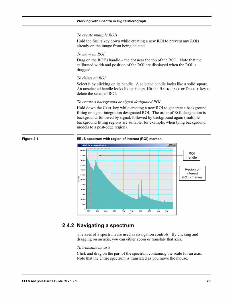
2.4.1 Regions of Interest (ROIs) A region of interest, or ROI, is used to indicate a location on a spectrum. An example of a spectrum with an ROI is shown in Figure 2-1. Normally there is only one ROI on a spectrum at a time, so each time you create a new ROI, the other ROI(s) are deleted. The easiest way to draw an ROI on a spectrum is to simply click on a spectrum with the pointer tool. If this does not produce an ROI on the spectrum, make sure that the pointer tool in the STANDARD TOOLS floating window is selected.

To create a wide ROI Click and drag on an image to create an ROI that is wider than a single channel.


Working with Spectra in DigitalMicrograph

To create multiple ROIs Hold the SHIFT key down while creating a new ROI to prevent any ROIs already on the image from being deleted.

To move an ROI Drag on the ROI’s handle – the dot near the top of the ROI. Note that the calibrated width and position of the ROI are displayed when the ROI is dragged.

To delete an ROI Select it by clicking on its handle. A selected handle looks like a solid square. An unselected handle looks like a + sign. Hit the BACKSPACE or DELETE key to delete the selected ROI.

To create a background or signal designated ROI Hold down the CTRL key while creating a new ROI to generate a background fitting or signal integration designated ROI. The order of ROI designation is background, followed by signal, followed by background again (multiple background fitting regions are suitable, for example, when tying background models to a post-edge region).

Figure 2-1 EELS spectrum with region of interest (ROI) marker.

2.4.2 Navigating a spectrum The axes of a spectrum are used as navigation controls. By clickidragging on an axis, you can either zoom or translate that axis.

To translate an axis Click and drag on the part of the spectrum containing the scale foNote that the entire spectrum is translated as you move the mouse

EELS Analysis User’s Guide Rev 1.2.1

ROI handle

Region of interest

(ROI) marker

ng and

r an axis. .

2-3


To zoom an axis Click and drag on the axis while holding down the CTRL key. Note that the x- and y-axes zoom in slightly different ways. The x-axis zooms around whichever point you click on, while the y-axis zooms around zero.

To restore a spectrum to its unzoomed view Right-click on the spectrum and select HOME from the pop-up menu to restore a spectrum to its default unzoomed view. Alternatively, use the ‘5’ key; if you use the number pad on a PC, make sure that NUM LOCK is turned on.

Turning auto-scaling on and off By default, a new spectrum window has auto-scaling switched on. This means that when the intensity increases or decreases, the y-axis automatically adjusts to scale to the new intensities. At times it is useful to turn this feature off, particularly when trying to focus a spectrum. Zooming or translating an axis automatically turns off auto-scaling for that axis. Restoring a spectrum to its unzoomed view automatically turns auto-scaling back on again for both axes.

Figure 2-2 Display options revealed by right-clicking on a spectrum.

Hints You can press and release the CTRL key without releasing the mouse to alternately zoom and then translate an axis.

When you click inside the axes of a spectrum, a new ROI is created on the image and the old ones are removed, but when you click outside the axis to navigate a spectrum, all the ROIs are left intact.

The LINE PLOT TOOLS floating window can still be used to navigate spectra, but it is generally faster to navigate spectra with the mechanisms described above.



Figure 2-3 Detailed menu revealed by right-clicking the color encoded legend.

2.4.3 Additional tools for manipulating single or multiple spectra Right-clicking your mouse with the cursor situated within a spectrum’s image window opens menu containing a number of useful display and editing options, as shown in Figure 2-2. Since multiple spectra can be displayed within a single image window, a color-coded legend provides the mechanism for specifying the current spectrum selected for adjustment (see Figure 2-3). Right-clicking on one of the titled legends reveals a menu containing additional items specific to the corresponding spectrum. When initiated in this way, the display command will be carried out (in the majority of cases) solely on the selected spectrum. Hence, spectrum-specific display parameters may be adjusted within an image window containing multiple spectra, enabling, for example, spectra with different intensity or energy ranges to be overlaid and rescaled with respect to each other for comparison.

The functions contained within the options list are as follows: CUT, COPY and PASTE: these commands carry out the same functions as in other Windows applications, and are described in detail the following section.

IMAGE DISPLAY initiates the IMAGE DISPLAY INFO dialog, allowing display and acquisition properties to be viewed and edited.

SHOW LEGEND reveals the color-coded legend bar within the image window.

HIDE LEGEND hides the legend list from the window display.

EELS Analysis User’s Guide Rev 1.2.1 2-5


SHOW [SPECTRUM NAME] displays the corresponding spectrum in the image window, in addition to any spectra already present. The displayed spectrum will have the same color as the corresponding legend tab.

HIDE [SPECTRUM NAME] conceals the corresponding spectrum from the image window. When a spectrum is contained within an image window but is hidden, the corresponding legend tab will not be colored.

HIDE OTHERS hides all spectra within the image window, with the exception of the currently selected spectrum.

SHOW ALL displays all the spectra contained within the image-window.

SEND BEHIND sends the corresponding spectrum to the back-most plane of the image window.

BRING TO FRONT brings the corresponding spectrum to the front-most plane of the image window.

ZOOM TO ROI rescales a spectrum with the region within the ROI zoomed to fill the entire spectrum window in both the x and the y directions. This is particularly useful when working with spectra containing a zero loss peak. It is a quick way of rescaling the spectrum to view the detail in the higher energy loss regions.

ZOOM VERTICALLY TO ROI performs a vertical rescaling of the spectrum with the intensity range falling within the ROI filling the image window, but keeping the horizontal scaling unchanged.

HOME DISPLAY returns the spectrum display to its default values.

ALIGN SLICE BY provides a sub-menu for aligning overlaid spectra with respect to the image window’s original spectrum. By CALIBRATION aligns the spectra by the x- and y-axis calibrated units. By UNCALIBRATED UNITS aligns the spectra by the channel number and uncalibrated counts.

ALIGN SLICE HORIZONTALLY BY provides a sub-menu for horizontally aligning overlaid spectra with respect to the image window’s original spectrum. The sub-menu items are as for ALIGN SLICE BY described above, except the alignment is performed horizontally only.

ALIGN SLICE VERTICALLY BY provides a sub-menu for vertically aligning overlaid spectra with respect to the image window’s original spectrum. The first two sub-menu items CALIBRATION and UNCALIBRATED UNITS are as for the ALIGN SLICE BY item described above, except the alignment is performed vertically only. Selecting INTEGRAL performs a y-axis alignment, rescaling the overlaid spectrum to have equal integral area to the original spectrum. The alignment may be performed over the full range of the image window, or over a discrete region denoted by an ROI. Selecting MAXIMUM rescales the vertical scaling (or region of, as defined by an ROI) to give equal maxima. Choosing BASELINE aligns spectra with respect to their vertical baselines.



RECALIBRATE SLICE performs an x-axis recalibration on the selected spectrum using the current spectrum display calibration. This command is useful for calibrating a spectrum with respect to another. For example, after manual alignment of an overlaid spectrum (by means of relaxing the horizontal constraints, see below), selecting this option recalibrates the foreground spectrum using the displayed scale.

HORIZONTAL CONSTRAINTS is a sub-menu facilitating adjustment of the horizontal constraints of the overlaid spectra. ATTACHED is the default setting, with the spectrum attached to the horizontal axis. DETACHED removes this constraint, allowing the selected spectrum to be moved freely with respect to the x-axis. To move the spectrum once DETACHED has been selected, double left-click on it and drag the mouse with the left button held down. Holding down CTRL while performing this action allows the horizontal scaling to be adjusted about the point shown by the vertical marker. BASELINE FIXED enables rescaling of the horizontal axis, with channel 0 remaining fixed. To adjust the spectrum once baseline fixed has been specified, double click on the spectrum then drag the mouse with the left button held down and the CTRL key depressed. Scale fixed performs the same operation as detached, but keeping the horizontal scaling fixed throughout.

VERTICAL CONSTRAINTS: this sub-menu provides the same function as described above for HORIZONTAL CONSTRAINTS, except in the sense of the y-axis.

DRAW STYLE: this sub-menu contains options for defining the draw style of the selected spectrum. Selecting DRAW FILL toggles the spectrum filling. DRAW LINE toggles the spectrum outline. FILL COLOR allows the color of the spectrum filling to be defined. LINE COLOR enables the color of the spectrum outline to be altered.

2.4.4 Moving spectra among image displays and to other applications To move spectra among image-displays within DigitalMicrograph, use the CUT, COPY, and PASTE items from the EDIT menu. They work very much the same way as they do in other Windows applications, placing copies of the selected data into a temporary storage area (CUT, COPY) and copying its contents to the foreground image-display (PASTE). If an ROI is placed on the spectrum, then these functions will operate on the sub-image as defined by the ROI bounds. You can paste data into a new image-display by pressing Ctrl-Alt-V simultaneously. You may also use the EDIT menu commands to transfer data from the foreground spectrum to any application capable of handling this information (for example, to your favorite spreadsheet application). If you wish to copy and paste the actual image representation within your spectrum’s image window, convert the spectrum to an RGB image by selecting CREATE IMAGE FROM DISPLAY in the OBJECT menu. An RGB image representation will be displayed in a new image window, which may then be transferred to other applications supporting this image type.


Performing mathematical operations on spectra

2.5 Performing mathematical operations on spectra

Mathematical operations are predominantly the domain of the PROCESS menu. For arbitrary mathematical manipulations of spectra, use the SIMPLE MATH… tool. The FFT and INVERSE FFT items facilitate custom processing involving Fourier transforms. Further spectral processing operations are found within the EELS menu item described in Chapter 3. Concatenation of spectrum segments acquired over different energy ranges is facilitated by SPLICE SPECTRA. Various preprogrammed digital filters are also available under the NUMERICAL FILTERS hierarchical menu. You can tailor these to your own needs via NUMERICAL FILTER SETUP….

2.6 Analyzing spectra

All spectrum analysis commands specific to EELS are grouped under the EELS menu. Use the items of this menu to extract sample-specific information from EELS spectra. Most of the items in this menu are self-explanatory and most will automatically prompt you for any required information missing from the EXPERIMENTAL CONDITIONS… dialog. As their names imply, these items help you COMPUTE THICKNESS of the probed area, REMOVE PLURAL SCATTERING from the spectrum, and perform QUANTIFICATION to establish the elemental composition of your sample and to determine the relative concentrations of the sample's constituents. All of these routines have been designed to give you quick, efficient access to such information, requiring a minimum of input from you and returning results within a few seconds. See the detailed descriptions of these items in Chapter 3 for limitations on their applicability.

2.7 Obtaining printouts

You will find printing commands situated in the FILE menu. Additionally, the contents of the REPORT sub-menu in the EELS menu provides the functionality to automatically format the spectrum within the image-display for printing as a report, together with the spectrum title and a text description of the experimental conditions and any signal extraction parameters specified. This sub-menu is explained in greater detail in Section 3.15.


3 The EELS menu

The EELS menu, shown in Figure 3-1, contains the analysis routines you need to extract physical data about your specimen from its EELS spectrum. Suitably acquired spectra will yield information such as relative specimen thickness and relative or absolute concentrations of chemical constituents. In contrast to the generic mathematical tools provided by the PROCESS menu, the routines of the EELS menu are specifically tailored to act on EELS spectra. Most of the routines are optimized for spectra obtained with Gatan EELS systems. The following sections give brief descriptions of the techniques used in each of the analysis routines. Further details may be found in the references listed in each section and in the book, Electron Energy-Loss Spectroscopy in the Electron Microscope 2nd Edition (Plenum Press, New York, 1996) by Egerton. This is an excellent text, which is considered widely as an essential reference book for anyone involved in EELS.

Figure 3-1 The EELS menu.


An important distinction between the analysis routines described in this chapter and the processing routines contained in the PROCESS menu is that analysis usually involves some level of data reduction. In other words, a small number of physical parameters are extracted from the spectrum data points, usually by way of least-squares fitting techniques. The significance of the derived parameters is typically indicated by the inclusion of an estimated uncertainty (or standard error) in the derived result, which is propagated from uncertainties in the original data points. Many of the routines below perform this propagation of uncertainties and indicate them by means of a ± value following the extracted quantity. The uncertainties in the measured EELS data points from which the error propagation proceeds are estimated assuming Poisson counting noise and a constant conversion factor from displayed detector counts to true primary beam electron counts. This conversion factor should have been measured for your system at installation, and will be initiated automatically when required.

Notes for Spectrum-Imaging Users

This version of EELS Analysis contains functionality for EELS analysis of spectrum-image datasets, enabling each of the items in the EELS menu to be applicable not only to single spectra, but also to spectrum-line-traces and spectrum images. This advance adds a new dimension of flexibility and potential to your EELS analysis capabilities, allowing complex EELS processing and analyses to be applied to entire spectrum-image datasets, enabling results previously only measurable as a single value to be computed and visualized as a line-plot or map. This functionality, referred to as EELS-SI Analysis throughout this documentation, requires the spectrum-imaging package to be installed in your version of DigitalMicrograph.

The EELS-SI Analysis routines use the same core algorithms as their single-spectrum counterparts, and are applied iteratively on a pixel be pixel basis. Hence for these analyses the output datasets have the same spatial dimensionality as the input data. Depending on the analysis performed, the output may also have identical or similar energy-loss dimensions as the input data, or alternatively will have no dispersion information at all. For example, consider an analysis that yields another spectrum as output when applied to a single spectrum (e.g. removal of plural scattering by Fourier deconvolution). When such an analysis is applied to a spectrum image, the output data will have the same dimensionality as the input dataset; that is, be a spectrum-image (e.g. a spectrum-image with plural scattering removed). Alternatively, in the case where an analysis produces a single value result when applied to a single spectrum (e.g. computing the relative thickness), this analysis will produce an image with the same spatial dimensionality as the source line-plot / spectrum image, but with no dispersion information (e.g. output a thickness plot or thickness map). Hence in this instance the output dataset will have one dimension less than the source data (for example, the output from a three-dimensional spectrum-image will be a two-dimensional map). It is useful to consider the dimensionality of the output dataset when choosing the optimal DigitalMicrograph tools for visualizing and exploring your results.


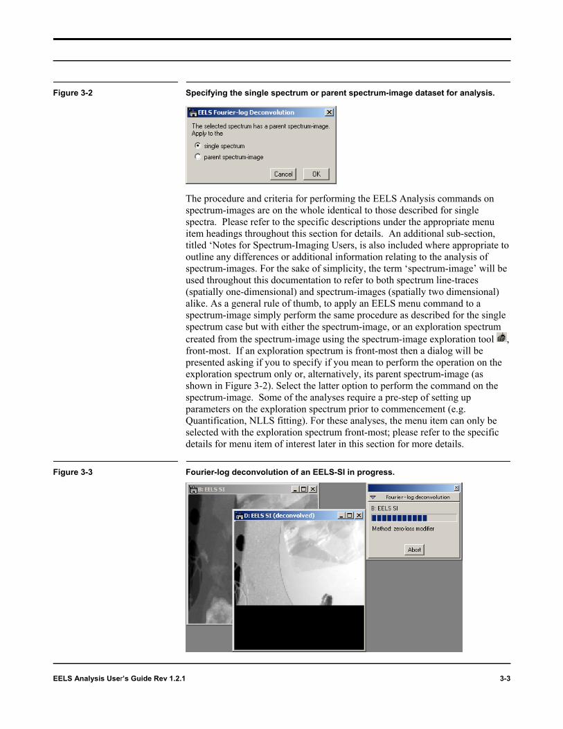
Figure 3-2 Specifying the single spectrum or parent spectrum-image dataset for analysis.

The procedure and criteria for performing the EELS Analysis commands on spectrum-images are on the whole identical to those described for single spectra. Please refer to the specific descriptions under the appropriate menu item headings throughout this section for details. An additional sub-section, titled ‘Notes for Spectrum-Imaging Users, is also included where appropriate to outline any differences or additional information relating to the analysis of spectrum-images. For the sake of simplicity, the term ‘spectrum-image’ will be used throughout this documentation to refer to both spectrum line-traces (spatially one-dimensional) and spectrum-images (spatially two dimensional) alike. As a general rule of thumb, to apply an EELS menu command to a spectrum-image simply perform the same procedure as described for the single spectrum case but with either the spectrum-image, or an exploration spectrum created from the spectrum-image using the spectrum-image exploration tool , front-most. If an exploration spectrum is front-most then a dialog will be presented asking if you to specify if you mean to perform the operation on the exploration spectrum only or, alternatively, its parent spectrum-image (as shown in Figure 3-2). Select the latter option to perform the command on the spectrum-image. Some of the analyses require a pre-step of setting up parameters on the exploration spectrum prior to commencement (e.g. Quantification, NLLS fitting). For these analyses, the menu item can only be selected with the exploration spectrum front-most; please refer to the specific details for menu item of interest later in this section for more details.

Figure 3-3 Fourier-log deconvolution of an EELS-SI in progress.


For the majority of analyses, once the spectrum-image analysis has been started the output results are displayed in their own image-windows. These image-windows are updated in real-time as the calculation proceeds. In addition, a palette containing a progress bar will be opened in the top-right corner of the screen for each analysis process, informing you of the state of progress of the computation (see Figure 3-3 above). For large spectrum-image datasets, computation times can be significant so please allow sufficient time for completion. In the event of an algorithm failure happening at a pixel, for example if the spectrum at that point is not suitable for the analysis in progress, then an appropriate failure message will be posted to the progress palette informing you of the nature of the error and the pixel co-ordinate. This will not halt the analysis, which will proceed to the next pixel until completion. Note that at any time during the computation, clicking the ABORT button positioned in the appropriate progress palette will halt the routine. Alternatively, closing all of the output windows associated with the computation will also halt the routine. The analysis routines run as background processes, allowing you to continue using DigitalMicrograph (or other applications) during lengthy computations, though please bear in mind performing other computationally intensive tasks will lengthen the overall computation time. Background processing offers the advantage of enabling you to view the output data as the computation proceeds to ensure that all is proceeding as expected. Further, you can batch process multiple analyses simultaneously, though bear in mind that computation times and memory requirements will increase appropriately. At completion of each computation, the total number of errors, if any, is posted in a dialog as a percentage of the total number of spectra analyzed.

Depending on the default image display settings (as specified in the Image DISPLAY INFO dialog, opened by selecting the IMAGE DISPLAY menu item in the OBJECT menu), or the type of data under analysis, the real time display may appear blank. There can be several reasons for this:

At an early stage of the computation, there may be insufficient information displayed to be included in the image survey contrast range. In these circumstances, wait sufficient time for the output data to reach a state of completion where the image survey contrast mechanism includes it in the displayed range (the display will be automatically refreshed as the computation proceeds). Alternatively, set the image’s SURVEY method to ‘WHOLE IMAGE’ via the IMAGE DISPLAY Info dialog.

If the output image is a spectrum-image, the energy-range being displayed may not contain any information. Use the SLICE floating palette, opened by selecting SLICE in the FLOATING WINDOWS sub-menu located in the WINDOWS menu, to change the displayed energy range to contain information. Alternatively, the spectrum-image exploration tool can be used to explore the output dataset. Please refer to the appropriate documentation for details on using these visualization tools.

The image may genuinely contain no information. In this instance, check the error text output in the progress floating-palette. If the algorithm is failing at each spectrum in the dataset then abort the process and i) ensure


the input data is appropriate for the analysis being performed and ii) specify alternate algorithm preference settings if appropriate before proceeding.

Figure 3-4 The EXPERIMENTAL CONDITIONS dialog.

3.1 Experimental Conditions

This item initiates the EXPERIMENTAL CONDITIONS dialog (Figure 3-4). Use this dialog to record the physical parameters of your particular acquisition setup. It is not necessary that you supply values for all the fields. However, in order to carry out quantitative elemental analyses, accurate values for the incident beam energy and the convergence / collection angles are required. When carrying out quantification, if any required fields have been left blank you will be prompted to enter these before continuing.

A tabbed dialog field labeled GLOBAL is presented in the EXPERIMENTAL CONDITIONS dialog, irrespective of whether an image-display is selected when initiating this command (see Figure 3-4). The data entered within this field are automatically copied to the IMAGE DISPLAY INFO tags of all subsequently acquired spectra. In addition, these settings are preserved from one DigitalMicrograph session to the next so that most need only be entered once. Note that the IMAGE DISPLAY INFO data stored with any spectra already acquired are not changed when you enter information within the GLOBAL field. To edit the data associated with a particular spectrum, initiate the EXPERIMENTAL CONDITIONS dialog with the desired spectrum image window selected. The dialog will now contain an additional tagged dialog field, labeled with the title of your spectrum. Values entered within this field will be particular to the corresponding spectrum. Note if the spectrum was imported from EL/P, the experimental conditions stored by EL/P will be read by EELS Analysis.


Calibrate Energy Scale

Figure 3-5 Calibrating the spectrum energy scale.

in

3.2 Cal

This calibrmodeselecpointabovethe fithe zecursorectanlow-echannreferesingl

Deperangeroutecorrechannleast scalespecispectthe recorreto the

3-2

Selected region of

terest (ROI)

ibrate En

command allowation of the sele is shown in Figted, an ROI shous to be used in t, this may be do

rst reference poiro-loss peak), hr to a second refgular marker, onergy vertical bel, and likewisence channel. Al

e channel ROI a

nding on wheth of channels, ths. For the singlesponding to the el. Use this mo

one feature of w in this mode, befying the disperrometer dispersictangular markesponding to the high-energy bo

Low-energy boundary

ergy Scale

s you to confirm and makected spectrum. An exampure 3-5. Before the CALIBld be placed on the spectr

he calibration procedure. ne by placing the cursor, nt (usually a feature of weolding down the left mouserence point before releasutlined by a discontinuousoundary of this rectangle the high-energy vertical dternatively, clicking once t that point.

er the region selected covee energy-scale calibration channel case, the proceduselected channel and also de if you know the disperell-defined energy-loss. W sure to take into consider

sion (the energy-scale scalon × binning). If more thar, the user is requested to low-energy boundary and,undary. The dispersion is

High-energy boundary

adjustmentle of the eneRATE ENERGYum to desigAs describedwith the poill defined ene button, aning. This w colored bo

denotes the lenotes the hon the spect

rs a single eroutine follore requests

the spectral sion accurat

hen calibraation any bie is defined n one channspecify the e in addition, then calcula

EELS Analysi

Energy calibrationdialog

s to the energy-scale rgy calibration SCALE command is

nate the reference in Section 2.4

nter tool selected, at ergy-loss, such as

d dragging the ill create a x as indicated. The ow-energy reference igh-energy rum will place a

nergy channel or a ws two different the energy dispersion in eV per ely and you have at ting the energy-nning applied when in units of el is highlighted by nergy-loss that corresponding ted based on the

s User’s Guide Rev 1.2.1

Splice

low and high marker energies and their separating interval. This mode is more suitable when the dispersion is not accurately known and two distinct features of known origin are present within the spectrum (e.g. the zero-loss peak and a sharp core loss feature of known energy-loss).


To recalibrate a spectrum-image, select this menu item with an active exploration spectrum selected from the spectrum-image front-most. The ENERGY-LOSS CALIBRATION dialog, shown above in Figure 3-5, will have an additional check box positioned at the bottom of the dialog titled ‘APPLY TO PARENT SPECTRUM-IMAGE’. This is selected by default. When this check box is selected, any recalibration applied to the exploration spectrum will also be automatically applied to the parent spectrum-image.

Figure 3-6 The SPLICE PREFERENCES dialog.

3.3 Splice

The items in the SPLICE sub-menu allow you to piece together a single continuous spectrum from two segments acquired over different (but overlapping) energy-loss ranges. The individual sub-menu items are described below.

3.3.1 Preferences… To change the default preferences used when performing the SPLICE SPECTRUM procedure (described below), select the PREFERENCES… menu item in the SPLICE sub-menu to open the preferences dialog (shown above in Figure 3-6). Via this dialog the user can specify the number of channels either end of the spectrum to discard, and also the number of overlapping channels to consider in the calculation of the scaling factor. Discarding the initial or final channels of a spectrum is useful for detectors that have a few channels of bad data at either end. The purpose of changing the number of channels used in calculating the scaling factor is to ensure that the splicing procedure does not produce artifacts. The default values for these parameters (4 for the number of channels to discard and 10 for the number of channels to consider in calculating the scaling factor) work well in most cases.


Splice

Figure 3-7 The SPLICE SPECTRUM… dialog.

3.3.2 Splice Spectrum… Select this item with one of the spectra you wish to splice front-most. You will then be presented with a dialog requesting you to select, from a list of dimensionally compatible spectra, the spectrum to splice with (see Figure 3-7 above). The routine uses the spectrums calibrated energy scales to decide how to concatenate the displayed segments, and as a result they must be properly calibrated for best results. If the data must be rebinned to a common dispersion before splicing, the software will ask the user for confirmation before proceeding. The overlapping channels of each pair of neighboring spectra are used to normalize the lower energy segment to the higher energy segment. The spliced result is then displayed in a new image window.

Note that you may see a distinct change in the signal to noise around the area where the two spectra are joined together. If the exposure time of the lower energy loss spectrum is less than that of the higher energy loss spectrum (a common situation due to the steep change in the background as a function of energy), then the lower energy loss portion will have a lower signal-to-noise ratio near the overlap region. The scaling will compensate for different exposure times, but it cannot compensate for the lower signal to noise in the spectrum acquired with a shorter exposure time.


To perform this command to splice a pair of spectrum-images, select the corresponding menu item with one of the datasets front-most. The routine will proceed as described above for the one-dimensional spectrum case. Observe that in addition to the suitability criteria described above for the single spectrum instance, the two datasets must also be of the same spatial dimensionality. Note also that the algorithm makes no consideration as to whether the two datasets are spatially registered; hence any drift alignment required between the datasets should be performed prior to performing this command.


Sharpen

Figure 3-8 The SHARPEN SPECTRUM PREFERENCES dialog.

3.4 Sharpen

The SHARPEN sub-menu contains items for recovering some of the spectral detail lost to the broad tails of the zero-loss peak. Specifically, the SHARPEN sub-menu items perform the following.

3.4.1 Preferences… Selecting this item opens the SHARPEN SPECTRUM PREFERENCES dialog, shown above in Figure 3-8. The SHARPEN SPECTRUM… routine, described below, requires a reference zero-loss profile as an input. The method for finding the zero-loss profile is specified in this dialog. If the SPECIFY A SEPARATE ZERO-LOSS PROFILE option is selected then the SHARPEN SPECTRUM… routine will ask you to specify explicitly the zero-loss profile to use from a list compiled from the dimensionally compatible open images. In this instance, the specified zero-loss profile is assumed to not need extraction and hence a model does not need to be specified in the ZERO-LOSS MODEL pull-down list (which will be inactive). Alternatively, if the EXTRACT THE ZERO-LOSS PROFILE USING THE MODEL BELOW option is specified then the routine will follow one of two routes. If the spectrum to be sharpened contains the 0 eV loss channel then it will attempt to automatically extract the zero-loss reference from this spectrum. If it does not, the routine will prompt you to specify an appropriate low-loss spectrum from which a zero-loss peak can be extracted. Whichever route is followed the zero-loss peak will be extracted using the model specified in the ZERO-LOSS MODEL pull-down list. For a more in depth description of the EELS ANALYSIS procedure zero-loss removal, please refer to EXTRACT ZERO-LOSS later in this section.


Sharpen

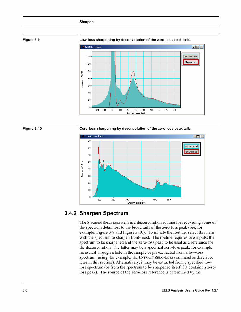
Figure 3-9 Low-loss sharpening by deconvolution of the zero-loss peak tails.

Figure 3-10 Core-loss sharpening by deconvolution of the zero-loss peak tails.

3.4.2 Sharpen Spectrum The SHARPEN SPECTRUM item is a deconvolution routine for recovering some of the spectrum detail lost to the broad tails of the zero-loss peak (see, for example, Figure 3-9 and Figure 3-10). To initiate the routine, select this item with the spectrum to sharpen front-most. The routine requires two inputs: the spectrum to be sharpened and the zero-loss peak to be used as a reference for the deconvolution. The latter may be a specified zero-loss peak, for example measured through a hole in the sample or pre-extracted from a low-loss spectrum (using, for example, the EXTRACT ZERO-LOSS command as described later in this section). Alternatively, it may be extracted from a specified low-loss spectrum (or from the spectrum to be sharpened itself if it contains a zero-loss peak). The source of the zero-loss reference is determined by the


Sharpen

preference set in the SHARPEN SPECTRUM PREFERENCES dialog - please refer to the PREFERENCES… section above for more details.

After some preparation of the reference zero-loss peak (explained below), the two inputs are Fourier transformed, the spectrum Fourier transform is divided by the zero-loss peak Fourier transform, and the result is inverse Fourier transformed to yield a spectrum largely free of the effects of the strong zero-loss peak tails. Once the procedure is complete, the sharpened result will appear in a new image-display. This routine checks the suitability of the inputs and takes specific measures to minimize noise amplification. The exact procedures are as follows:

Check inputs. The program first checks that the front-image contains spectrum data. If the spectrum contains a zero-loss peak, and if told to do so, it then extracts the zero-loss peak from the spectrum using the zero-loss model specified in the SHARPEN SPECTRUM PREFERENCES dialog (please refer to EXTRACT ZERO-LOSS later in this chapter for details). Otherwise, it uses the zero-loss peak as specified by the user, which must be an open and calibrated single spectrum containing the 0eV channel within its range. Finally, it checks that the specified zero-loss spectrum is, in fact, a symmetrical zero-loss peak. If not, the routine posts a suitable warning.

Ensure identical dispersions Based on the dispersion of the spectrum to be sharpened, the zero-loss spectrum is interpolated to the same eV / ch if required. If the ratio of the dispersions exceeds a factor of two then a warning is posted to alert the user that the accuracy of the routine may be compromised.

Determine size of Fourier transform to be used. Based on the range of non-zero channels in each of the inputs, the routine next establishes the number of channels needed for the Fourier transform computations. In order to provide enough empty buffer channels to allow for smooth extrapolations, the routine chooses the smallest power of 2 that is at least 1.5 times the number of non-zero channels in the selected spectrum.

Remove truncation discontinuities in the target spectrum. To avoid artifact ringing due to truncation, the routine next smoothly extrapolates the endpoints of the spectrum to be sharpened to zero using a cosine-bell function.

Prepare deconvolution function. Because of the noise in any measured spectrum, a simplistic deconvolution of the entire zero-loss profile will cause the Fourier components of the noise to dominate those of the deconvolved spectrum, resulting in a useless result. The important point is not to try to recover more than the inherent resolution of the spectrum, which is reflected in the steepness of the central portion of the zero-loss peak. The method used here is to fit a Gaussian to the narrow central portion of the zero-loss peak and to replace that portion of the peak with a δ-function of equal area. The Gaussian portion is isolated by fitting a Gaussian to


Sharpen

the zero-loss peak data over the range that is within 90% of the zero-loss peak amplitude (minimum of three channels). The fit is subtracted, negative residual values being set to zero. The total count differential between this processed result and the original deconvolution function is placed in the single channel, which previously contained the maximum of the zero-loss peak. This modified deconvolution function is then normalized to an integral of 1, and it is shifted (with endpoint wraparound) so that the ∂-function peak is in channel 0. These last two steps ensure that the deconvolved spectrum contains the same number of counts as the original and that there is no horizontal offset between them.

Perform Fourier transform manipulations. The two inputs suitably prepared, the routine next Fourier transforms them using a Fast Fourier Transform (FFT) algorithm. It divides the spectrum transform by the deconvolution function transform (using complex arithmetic), and inverse Fourier transforms the result.

Output result. Finally, the resultant deconvolved spectrum is displayed in a new image-display.


To sharpen a spectrum-image dataset, select the SHARPEN SPECTRUM menu item with either the spectrum-image or an associated exploration spectrum taken from the spectrum-image front-most. If an exploration spectrum is front-most, specify the parent spectrum-image as the input dataset when prompted. If SPECIFY A SEPARATE ZERO-LOSS PROFILE is selected in the SHARPEN SPECTRUM PREFERENCES dialog, you will then be requested to specify a suitable single spectrum zero-loss profile to be used in the sharpen algorithm. If EXTRACT THE ZERO-LOSS PROFILE USING THE MODEL BELOW is selected in the preferences dialog, the routine will follow one of the following two routes. If the spectrum-image contains the 0 eV channel, the routine will extract the zero-loss profile from the spectrum-image itself on a spectrum-by spectrum basis. If the spectrum-image does not contain the 0 eV channel, you will be requested to specify a low-loss single spectrum that is suitable for the zero-loss profile to be extracted from. This profile will then be applied to each spectrum in the dataset. Note that for this routine the output dataset has identical dimensionality to the input dataset.

Figure 3-11 The BACKGROUND MODEL DEFAULTS dialog.


Background Model

3.5 Background Model

The BACKGROUND MODEL sub-menu facilitates fitting, extrapolation and subtraction of the characteristic energy-loss background from your spectrum. The sub-menu items are described as follows.

3.5.1 Preferences… A number of models may be used to model the energy-dependence of the characteristic background signal. Selecting this sub-menu item opens the BACKGROUND MODEL DEFAULTS dialog, through which the default background model may be defined (Figure 3-11). Supported models include power-law, polynomial or log-polynomial functions. If polynomial or log-polynomial is selected, the user may also specify the degree polynomial to be used. The model specified in this dialog will be applied when creating all subsequent background models. In general, the power-law background model is the most robust and gives the most reasonable fit for typical EELS edge data. However, if an edge is in the low-loss regime (below about 100 eV), or if another edge precedes it closely, then the simple power-law model will likely fail. It is often possible to tell by eye whether the model provides an accurate fit; for example, if the extrapolated background intersects the spectrum soon after the edge then most likely the background fit is inadequate and an alternative model could yield a better fit. In the case of a low-loss background, a polynomial or log polynomial model function will sometimes yield better results. For example, see the following reference:

A.R. Wilson, "Detection and quantification of low energy, low level electron energy loss edges", Microsc. Microanal. and Microstruct., 2 (1991) 269.

Since the polynomial and log-polynomial background models are far less robust and require an experienced eye, it is recommended that the power-law model be used first and foremost.

3.5.2 Extrapolate Background Use this command to model and extrapolate the characteristic background under an edge (Egerton, pp. 269-277). The background model applied is taken from the default setting as specified in the BACKGROUND MODEL DEFAULTS dialog as described above. Once created, it may be adjusted using the CHANGE CURRENT MODEL… function described next in this section. In general, a power-law model of the form AE -r is most commonly applied, and it is recommended that inexperienced users apply this model since it is found to yield the most satisfactory results in the majority of cases.


Background Model

Figure 3-12 Power-law background modeling under a core-loss edge.

Background fitting region

Core-loss edge with background removed

Extrapolated background model

To extrapolate the background below a core-loss edge, first define the portion of the pre-edge background to be modeled and extrapolated by selecting a rectangular ROI over the desired range. To do this, with the pointer tool selected, hold the left mouse button; drag the mouse until the region is defined and then release. Typically, a range starting 40-50 eV before the edge threshold and 25 eV in width serves well for this purpose. A good account of how to choose the optimal background fitting region widths and positioning for a given edge may be found in the following references:

1. Liu D-R. and Brown L.M., “Influence of some practical factors on background extrapolation in EELS quantification”, J. Microsc. 147 (1987) 37-49

2. Joy D.C. and Maher D.M., “The quantitation of electron energy loss spectra”, J. Microsc, 124 (1981) 37-48

Please note that the routine requires the spectrum energy scale to be roughly correct to give reliable results. It is particularly important to confine your selection to spectrum ranges that exhibit true power-law behavior in order to get a good fit when using the power-law model, for example. This means that intervals which contain residual structure from preceding or overlapping edges, or which include pre-edge structure of the leading tail of the edge in question, should be avoided. Once you have highlighted the background fit interval, select EXTRAPOLATE BACKGROUND. Note that as an alternative to the above, you can also create a background fit region by simply holding down the CTRL key and left-click dragging over the background fit region on the spectrum. In either instance, the routine then does the following:

1. Fit the background function to the selected background data over the specified fit region.


Background Model

2. Extrapolate the background fit to the last channel of the spectrum to obtain a full background model.

3. Subtract the background model from the original spectrum.

4. Display both the background model and the background-subtracted spectrum within the original spectrum’s image-display.

Note that this routine will not alter the original spectrum in any way. Additionally, the selected background-fitting region, which may be described as ‘active’, can be altered post-modeling. To do this, place the cursor within the ROI labeled BKGD and, holding the left-hand mouse button, reposition the background-fitting region by dragging it to a new position. Alternatively, left clicking on the low-energy or high-energy boundaries and dragging allows the fitting region to be resized. The arrow keys can be used to the same effect, with the left and right keys moving the window left and right by single channel increments respectively, and the up and down keys increasing and decreasing the width of the fitting region. The modeled background contribution and background-subtracted spectrum are recalculated and redisplayed as the model parameters are altered, making it very convenient to interactively modify the background fit interval to get the best possible background fit.

To extract either the background model or subtracted edge and place it in its own image-display, use the EXTRACT BACKGROUND MODEL or SUBTRACT BACKGROUND commands respectively as described later in this section.

3.5.3 Change Current Model This routine allows the attributes for an existing background model to be altered. To initiate this function, select the menu item with the appropriate spectrum front-most. A dialog similar to the BACKGROUND MODEL DEFAULTS dialog, shown in Figure 3-11, will open allowing you to alter the model attributes while viewing the effect of any changes on the spectrum. Note that changes initiated here will apply to the selected spectrum only and will have no effect on the global background model defaults (see PREFERENCES… above for details on changing the global background defaults). To apply any changes made press OK, to revert to the original state press CANCEL.

3.5.4 Extract Background Model Use this command to extract an ‘active’ background model and display it in a new image-window. To initiate this routine, select the menu item with a spectrum front-most with an ‘active’ background model in place. The routine will duplicate the background model, displaying it in a new image-window. Note that the extracted background model will be inactive, and hence will not change in response to any alteration of the background fitting or modeling parameters on the source spectrum.


Background Model


To extract fit and extract the background model on a pixel-by-pixel basis from a spectrum-image, perform the ROI set-up procedure, as described above for the single spectrum case, on an exploration spectrum taken from the spectrum-image. Select the EXTRACT BACKGROUND MODEL menu item and specify the parent spectrum-image for analysis when prompted. The background fit will then be applied on a pixel-by-pixel basis on the spectrum-image using the fitting region and background model as specified for the exploration spectrum. The background model dataset, which will have the same dimensionality as the input data, will be displayed in a new image-window. Note that log-polynomial backgrounds, and polynomial background models of order greater than 1, are not supported for spectrum-imaging use.

3.5.5 Extract Background Subtracted Signal Use this command to permanently subtract the ‘active’ background model from the spectrum, yielding the background-extrapolated signal displayed in a new image-window. To initiate this routine, a spectrum must be front-most with an ‘active’ background model present. The routine duplicates the background subtracted core-loss signal, and displays it in a new image-window. Note that the extracted background-subtracted signal will be inactive, and hence will not change in response to any alteration of the background fitting or modeling parameters on the source spectrum.


To perform background subtraction on a spectrum-image, perform the ROI set-up procedure, as described above for the single spectrum case, on an exploration spectrum taken from the spectrum-image. Select the EXTRACT BACKGROUND SUBTRACTED SIGNAL menu item, and specify the parent spectrum-image for background subtraction. The background subtraction will then be applied on a pixel-by-pixel basis on the spectrum-image using the fitting region and background model specified on the exploration spectrum. The background subtracted signal dataset, which will have the same dimensionality as the input data, will be displayed in a new image window. This routine applied is identical to the Create Background Subtracted SI command in the SI menu. Note that log-polynomial backgrounds, and polynomial background models of order greater than 1, are not supported for spectrum-imaging use.


Sum Overlaid Spectra

Figure 3-13 Example of the SUM OVERLAID SPECTRA command.

Overlaid spectra

SUM OVERLAID SPECTRA

Summed spectra

3.6 Sum Overlaid Spectra

Use this menu item to sum multiple, overlaid spectra that are displayed in the same image-display. The spectra are summed as-displayed, and hence may be manually aligned beforehand with respect to their dispersion scales using the standard DigitalMicrograph tools for manipulating spectrum slices. Please refer to Section 2.4.3, in particular the HORIZONTAL CONSTRAINS sub-section, for further details on manipulating spectrum slices. This command is therefore useful for the addition of separately acquired spectra, possibly with different dispersions, and automatically takes into account any changes in horizontal offset or scaling that the user may have applied to yield a single spectrum displayed in a new image-display.

The output spectrum is automatically cropped to the energy-range common to the overlaid spectra. If necessary, the spectra are also rebinned to a common dispersion as determined by the spectrum corresponding to Slice 0. Note that to perform this procedure the front-most image-display must contain two or more visible spectra, with at least two channels of overlap. Any hidden spectrum slices will be excluded from the procedure. In addition, any change in vertical scaling is ignored, hence allowing the user to manipulate the intensity scales of the individual spectra as an aid to manual alignment, whilst preserving the counting statistics in the final summed spectrum.

To perform this operation, do the following:

1. Place the spectra to be summed into a single image-display, as shown in Figure 3-13. To achieve this, cut and paste, or right-click drag, the spectra into a single line-plot image-display (e.g. the image-display of one of the spectra of interest). Please refer to Section 2.4.4 for more details on displaying multiple spectra in a single image-display. If the spectra are calibrated they will be automatically aligned with respect to their energy-loss, regardless of their dispersion.


Numerical Filters

2. Manually align the spectra by shifting them horizontally. To do this:

a. If the line-plot’s image-display legend is not already visible, right click on the image-display and select SHOW LEGEND.

b. Right click on the appropriately colored legend corresponding to the spectrum slice you wish to align, and select DETACHED in the HORIZONTAL CONSTRAINTS sub-menu.

c. Left click on the spectrum display to create a solid, vertical marker. Left-click dragging on this marker will now allow you to offset the spectrum slice horizontally. Holding down CTRL while performing this action will allow you to change the horizontal scaling.

Repeat for all of the spectrum slices you wish to align.

3. Once the spectra are aligned to your satisfaction, select the SUM OVERLAID SPECTRA menu item with the image display front-most. The summed spectrum will be displayed in a new image window.

Figure 3-14 The NUMERICAL FILTERS PREFERENCES dialog.

3.7 Numerical Filters

The NUMERICAL FILTERS hierarchical menu provides a variety of filtering routines, primarily for noise and background reduction. These filters may be carried out on single spectra, spectrum line-traces or EELS / EFTEM spectrum-images alike.

3.7.1 Preferences… The PREFERENCES… item initiates a dialog for specifying the various filter parameters used in these operations (see Figure 3-14). Numerical filtering is of interest for noise and background reduction, and additionally for revealing


Numerical Filters

features or variations that may normally be obscured by the accompanying electron energy-loss signal. First and second difference filters are particularly useful within this context. Hence the main applications of the NUMERICAL FILTERS are

1. Background reduction to make edge signals easier to distinguish, and

2. Transformation of previously acquired reference spectra (such as those of the EELS atlas) for comparison to newly acquired spectra.

All filter parameters are specified in eV, the calibrated unit in the energy-loss plane, rather than in channels. The actual number of channels of shift or averaging is thus a function of the spectrum eV/channel. The significance of each filter parameter and its precise interpretation for each filter routine is described fully under the appropriate subheading of this section.

Two buttons are also provided to allow the user to quickly set preset default filter values appropriate for the mode in which the spectral information was acquired. The HIGH-RESOLUTION button sets values suitable for analysis of spectral information acquired in spectroscopy mode (as a spectrum, spectrum line-trace or spectrum-image). Alternatively, the LOW-RESOLUTION button sets values suitable for lower-spectral resolution information, acquired, for example, as an EFTEM spectrum-image. The default values for these options may in turn be altered to suit preference; selecting the button situated next to the appropriate default setup button opens a dialog containing the relevant settings for modification. For advanced users, removing the NUMERICAL FILTERS tag group found in the GLOBAL INFO… menu will restore the original, as-installed default values.

The effect of each filter is described below.

3.7.2 Smooth (low-pass) The smoothing filter averages out some of the noise in a spectrum and places the result in a new display, leaving the original data unchanged. It acts by replacing the value in each spectrum channel by the average number of counts per channel in an interval w eV wide and centered on the channel in question. In the case of the specified energy interval corresponding to an even number of channels, an extra channel is added and only half of the contribution of the two end channels considered, mimicking the specified smoothing interval without introducing a resultant energy-shift into the final spectrum / spectrum-image. The width, w, of the averaging interval is set under SMOOTH (LOW-PASS) in the FILTER SETUP dialog. For the smooth filter (and all the following filters), endpoints are handled by repeating the first and last values in the spectrum as required.

3.7.3 Structure (high-pass)


The structure filter isolates most of the interesting features in a spectrum and places the result in a new display, leaving the original data unchanged. It acts by subtracting a heavily smoothed copy of a spectrum from itself, thereby

Numerical Filters

greatly reducing the intensity in the slowly varying portions, such as the smooth power-law background. The smoothed copy is obtained via channel averaging over an interval of specified width, as for the SMOOTH filter. The width in eV, w, of the averaging interval is set independently of the smoothing width under STRUCTURE (HIGH PASS) in the FILTER SETUP dialog.

3.7.4 First derivative This item calculates an approximate first derivative of the foreground spectrum and places the result in a new display, leaving the original data unchanged. The routine first smoothes the data over an interval w eV wide, then it calculates the difference between values dE eV apart and places the result in the channel midway between two. The parameters w and dE are set under the FIRST/LOG DERIVATIVE heading of the FILTER SETUP dialog. Finally, the spectrum is divided by w + dE to yield an approximation of the first derivative with respect to energy.

3.7.5 Log derivative This item calculates an approximate logarithmic derivative of the foreground spectrum and places the result in a new display, leaving the original data unchanged. The routine performs the same procedure as FIRST DERIVATIVE but adds one final step; dividing the result by the original spectrum.

3.7.6 Log-log derivative This item calculates the approximate derivative of the foreground spectrum as plotted on a log-log scale and places the result in a new display. In regions dominated by the power-law background, the resultant value reflects the local power-law exponent. This is why the transform is sometimes referred to as an R-plot. The routine performs the same procedure as LOG DERIVATIVE but adds one final step; multiplying the result by the energy-loss.

3.7.7 Second derivative This item calculates an approximate second derivative of the foreground spectrum and places the result in a new image display. The routine averages over an interval w+ eV wide and subtracts half the aver-ages in two adjacent "wings" of width w-, as illustrated and set under the SECOND DERIVATIVE heading in the FILTER SETUP dialog. Finally, the spectrum is divided by the squared sum of w+ and w- to yield an approximation of the second derivative with respect to energy.


Zero-Loss Removal

Figure 3-15 The ZERO-LOSS EXTRACTION PREFERENCES dialog.

3.8 Zero-Loss Removal

The ZERO-LOSS REMOVAL sub-menu contains items for modeling and extracting the zero-loss peak from low-loss spectra. The individual menu items are described as follows.

3.8.1 Preferences… Select this menu item to open the ZERO-LOSS REMOVAL PREFERENCES dialog, shown above in Figure 3-15. This dialog contains the preferences used by the EXTRACT ZERO-LOSS command described below. The current zero-loss model is specified in the ZERO-LOSS MODEL pull down list. This list contains all the preset zero-loss models, described in detail in the following sub-section, in addition to any user-defined models. Quantities output, in addition to the extracted zero-loss peak, can be specified in the OUTPUT group of options at the bottom of the dialog. Selecting the output INELASTIC CONTRIBUTION tick-box results in the inelastic contribution being computed and displayed. If the output EXTRACTED SIGNAL INTEGRAL(S) box is ticked then the routine will also output the zero-loss (and, if specified as above, inelastic) signals integrated in energy-loss. Selecting output MEAN ZERO-LOSS ENERGY results in the mean energy-loss of the extracted zero-loss peak being output; this quantity is useful, for example, for removing any zero-loss drift from a spectrum-image acquisition (see CORRECT ZERO-LOSS CENTERING (SI USERS ONLY) below for details).

3.8.2 Extract Zero-Loss The EXTRACT ZERO-LOSS command extracts the zero-loss peak from the front-most spectrum, and displays the peak in a new image-window. If specified in the REMOVE ZERO-LOSS PREFERENCES dialog, as described above, the inelastic signal and/or the zero-loss and inelastic signal integrals are also output. To initiate this routine, select the EXTRACT ZERO-LOSS menu item with the image-window containing the low-loss spectrum of interest positioned front-most.

The requirements of this routine are:

1. The spectrum's energy scale must be calibrated.


Zero-Loss Removal

2. It must be a low-loss spectrum, i.e. it must include the zero-loss peak.

3. The zero-loss peak must not be too close to the left edge of the detector i.e. its leading tail should not be truncated.

If the first requirement is not met, the routine will post a suitable alert and you will need to calibrate the energy scale before proceeding further. If the last requirement is not met, the procedure will continue but bear in mind that truncation of the zero-loss leading tail may be detrimental to the accuracy of the results produced.

The extracted zero-loss peak is displayed (in addition to the inelastic component, if specified) in a new image-display, and any supplementary information posted as appropriate. The extracted zero-loss peak serves as a convenient input for the SHARPEN RESOLUTION routine (see Section 3.4 above).

The routine has a number of pre-defined routines for extracting the zero-loss peak. In addition, user defined custom models can be added for further flexibility (as described later in this section). The preset zero-loss models are described below:

Reflected tail This model is fast, robust and well suited to the majority of cases. It is therefore recommended for general use. Because the tails of the zero-loss peak can contain a substantial number of counts relative to the loss part of the spectrum, it is important to take account of them when performing the zero-loss peak separation. In the reflected tail model this is achieved by assuming the zero-loss tails are relatively symmetric and uses a reflection of the left-side tail to model the tail on the energy-loss side. Specifically, it a) replicates the spectrum from the first channel to a cutoff point at 1.5 FWQM (full width at quarter maximum) before the peak, b) reflects the replicated tail about the zero-loss maximum, c) removes any mean background offset from the reflected tail, measured from the region on the low-energy loss side below 3*FWQM from the zero-loss center, using at most the first 5 % of non-zero channels in the spectrum and at least the first 3 non-zero channels d) vertically scales the reflected tail using the ratio of the sum of the overlapping 3 channels (if possible, scaling down to 1 channel with decreasing FWQM) at the low-loss cutoff and the high-loss join point, e) attenuates the reflected tail at the first non-positive channel and f) replaces the high-loss spectrum above the join point with the reflected tail to yield the zero-loss peak. g) This zero-loss model is subtracted from the original spectrum to yield the inelastic signal, and all channels from the beginning of the spectrum range to the rightmost negative count residual in the inelastic signal within the zero-loss extrapolation range are set to zero then finally, i) the inelastic signal is then subtracted from the original spectrum to yield the output zero-loss peak. [Note for advanced users: the reflected tail cutoff point may be varied by opening EELS>SETTINGS>ZERO-LOSS MODELS>REFLECTED TAIL in the GLOBAL INFO tags, and entering an appropriate value in units of FWQM in the REFLECTED TAIL cut-off field. Additionally, the post-extrapolation clean-up


Zero-Loss Removal

step g) can be disabled by setting the PERFORM POST-FIT CLEANING tag to FALSE].

Fitted log. tail This simple model fits and extrapolates a logarithmic function to model the +ve energy-loss tail of the zero-loss peak. Since the model is relatively simple, and as the fitting range may be user specified, it is both robust and versatile. On initiating the routine the user is requested via a dialog to specify the log. model fitting range. The fit range is measured in eV with respect to the zero-loss peak maximum (by default from 2eV to 4eV loss). The dialog also contains checkboxes for specifying i) to have the specified range remembered for future use, and ii) to suppress displaying the dialog in future computations. The routine then proceeds as follows: a) the position of the zero-loss peak maximum is measured, b) the fit range is replicated and a log. transform is applied c) a straight line is least-squares fitted over the fit range(note all non-positive channels are ignored), d) using the fit coefficients, the +ve loss tail is then modeled and extrapolated over the spectrum’s energy-loss range, and then e) the spectrum and logarithmic tail are replicated and spliced at the fitting mid-point to yield the extracted zero-loss peak . e) This zero-loss model is then subtracted from the original spectrum to yield the inelastic signal, and all channels from the beginning of the spectrum range to the rightmost negative count residual in the inelastic signal within the specified log. fitting range are set to zero and then, finally, f) the inelastic signal is then subtracted from the original spectrum to yield the output zero-loss peak. [Note for advanced users: The post-extrapolation clean-up steps e-f) can be disabled by opening EELS>SETTINGS>ZERO-LOSS MODELS>FITTED LOG. TAIL in the GLOBAL INFO tags, and setting the PERFORM POST-FIT CLEANING tag to FALSE. Additionally, setting the DON’T SHOW RANGE DIALOG tag to FALSE will re-enable the fit range dialog if disabled].

Fit Pre-Measured Zero-loss This routine fits a user specified zero-loss profile to the zero-loss peak of the selected spectrum. The algorithm is relatively simplistic, being both robust and relatively quick. The routine proceeds as follows: a) It first requests the user to specify the reference zero-loss peak, which should be a single spectrum containing the zero-loss peak only and, ideally, acquired at the same dispersion in order to have contain same detector response characteristics as the object spectrum (i.e. have the same degree of spectral smoothing arising from the point-spread function), b) the reference zero-loss peak is rebinned to the same dispersion as the low-loss spectrum if necessary, c) the zero-loss center position of both the reference spectrum and the low-loss spectrum are found by least-squares fitting a Gaussian function to their zero-loss peaks over a fitting region (by default) of 2 HWHM on the low-energy loss side to 1 HWHM on the high energy loss side (where HWHM is the half-width half maximum of the zero-loss peak), d) the reference zero-loss peak is aligned with the low-loss zero-loss peak using sub-channel interpolation, e) an intensity scaling factor is established by computing the intensity ratio over a fitting region, by default from 1.75 to 3eV in loss measured with respect to the zero-loss maximum, and then f) the spectrum is replicated up to the fitting mid-point, and is spliced with


Zero-Loss Removal

the scaled aligned zero-loss reference beyond this point up to the first –ve channel (or reference array end) to give the elastic peak. g) The elastic peak is subtracted from the low-loss spectrum to yield the inelastic signal, h) all channels from the beginning of the spectrum range to the rightmost negative count residual in the inelastic signal (up to 5eV loss by default) are set to zero, i) the inelastic signal is then subtracted from the original spectrum to yield the output zero-loss peak. [Note for advanced users: the Gaussian and zero-loss intensity ratio fit range may be varied by opening EELS>SETTINGS>ZERO-LOSS MODELS>FIT PRE-MEASURED ZERO-LOSS in the GLOBAL INFO tags, and entering an appropriate value in units of eV in the FIT START and FIT END fields as appropriate. Additionally, the post-extrapolation clean-up steps g-i) can be disabled by setting the PERFORM POST-FIT CLEANING tag to FALSE].

2 Gaussian fit The ‘2 Gaussian’ model uses least-squares fitting to fit two Gaussian functions to the zero-loss peak. It is reasonably robust, but is not well suited to zero-loss peaks with long tails arising from high detector point-spread function. Specifically, it a) fits a single Gaussian model to the zero-loss peak to accurately measure the zero-loss center and half width half maximum (HWHM), then b) attempts to fit two Gaussian models to the spectrum over a fitting region, by default from –6 to +3 times the zero-loss HWHM either side of the zero-loss center. To ensure a sensible fit, one of the Gaussian models has its center position constrained to the zero-loss center, whilst the second has its width constrained to that of the zero-loss peak. c) The sum of the Gaussian models is subtracted from the original spectrum to yield the inelastic signal. All channels from the beginning of the spectrum range to the rightmost negative count residual in the inelastic signal within the zero-loss extrapolation range are set to zero. d) Finally, the inelastic signal is then subtracted from the original spectrum to yield the output zero-loss peak. [Note for advanced users: the Gaussian fit ranges to the left and right of the zero-loss center can be adjusted by opening EELS>SETTINGS>ZERO-LOSS MODELS>2 GAUSSIAN in the GLOBAL INFO tags, and entering an appropriate value in units of HWHM in the appropriate fields. Additionally, the post-fitting clean-up step c) can be disabled by setting the PERFORM POST-FIT CLEANING tag to false].

Gaussian & Lorentzian fit This model uses least-squares fitting to fit the sum of a single Gaussian and a Lorentzian function to the zero-loss peak. The Lorentzian function has long tails and hence this model is suited to spectra recorded on detectors with high point-spread. Specifically it a) fits a single Gaussian to the zero-loss peak to accurately measure the zero-loss center and half width half maximum (HWHM), then b) attempts to fit a Gaussian and a Lorentzian model to the spectrum over a fitting region, by default from –6 to +3 times the zero-loss HWHM either side of the zero-loss center. An AMOEBA simplex algorithm is used to perform the least-squares fitting. c) The sum of the Gaussian models is subtracted from the original spectrum to yield the inelastic signal. All channels from the beginning of the spectrum range to the rightmost negative count


Zero-Loss Removal

residual in the inelastic signal within the zero-loss extrapolation range are set to zero. Finally, the inelastic signal is then subtracted from the original spectrum to yield the output zero-loss peak. [Note for advanced users: the fitting range to the left and right of the zero-loss center can be adjusted by opening EELS>SETTINGS>ZERO-LOSS MODELS>GAUSSIAN & LORENTZIAN in the GLOBAL INFO tags, and entering an appropriate value in units of HWHM in the appropriate fields. Additionally, the post-fitting clean-up step c) can be disabled by setting the PERFORM POST-FIT CLEANING tag to false].

Gaussian & Lorenzian2 This model uses least-squares fitting to fit the sum of a single Gaussian and a Lorentzian function squared to the zero-loss peak. The squared Lorentzian has extended tails to suit detectors of high point-spread, but less so than the preceding model. The fitting procedure is identical to that described above for the Gaussian & Lorentzian model.

Maxwell-Boltmann This model fits a Maxwell-Boltzmann distribution of the form

×−

= − TEAEI 5106.8

exp)(

where I is intensity, E is energy-loss, A a constant, and T the emitter temperature (in K). The model produces an asymmetric distribution and is suitable for spectra acquired using a cold-FEG source. By default, the start value of T is 800°K. The fitting procedure is identical to that described above for the Gaussian & Lorentzian model. This model fits the sum of a Maxwell-Boltzmann distribution, described above, and a Lorentzian function that models the extended zero-loss tails. This model is therefore suited to asymmetrical distributions recorded using a detector with high point-spread function. By default, the start value of T is 800°K. The fitting procedure is identical to that described for Gaussian & Lorentzian above.

It should be noted that all the preset zero-loss fitting routines find the zero-loss peak initially by searching for the maximum intensity peak after applying a filter that emphasizes features as a function of their distance from the 0 eV channel (as calibrated). Hence the routines should successfully locate the zero-loss peak even for very thick samples providing they are reasonably well calibrated (the zero-loss peak should be located to within approximately ±10eV for spectra from thicker regions, with larger error margins for spectra from thinner regions).

User defined models can be added to the zero-loss model list by creating and installing a custom script written in the DigitalMicrograph script language, details of which are given in Section 4.2. Note that any custom zero-loss models will also appear in the zero-loss model pull down list for other routines that require zero-loss extraction – for example, the COMPUTE THICKNESS routine described below.


Compute Thickness

3.8.3 Correct Zero-Loss Centering (SI users only) Select this item to correct the zero-loss peak centering with respect to the calibrated zero-loss center from a spectrum line-trace or spectrum-image using a pre-measured zero-loss position map. This procedure is useful, for example, for removing any zero-loss drift from arising from chromatic effects or microscope high-tension instability.

To perform this procedure, select this menu item with the spectrum-image front-most. The routine will then prompt you to specify the corresponding zero-loss drift map from a list of the open images that are dimensionally compatible. The selected image should contain the calibrated deviation of the input data’s zero-loss peak position; the mean zero-loss energy output of the EXTRACT ZERO-LOSS routine, as described above, is ideal for this purpose. If the zero-loss position map is calibrated in incompatible units then an appropriate error will be posted to inform you that the calibrated units will be ignored. In this event a shift calculated from the deviation of the uncalibrated zero-loss position value from the mean of the zero-loss position map will be applied. Once complete, the corrected spectrum-image will be displayed in a new image-window.


To perform zero-loss extraction from a spectrum-image, select the EXTRACT ZERO-LOSS menu item with either the spectrum-image or associated exploration spectrum taken from the spectrum-image front-most. If an exploration spectrum is front-most, specify the parent spectrum-image as the input dataset when prompted. Note that the outputted extracted zero-loss and inelastic signal datasets have identical dimensionality as the input dataset. If output EXTRACTED SIGNAL INTEGRAL(S) is specified in the ZERO-LOSS REMOVAL PREFERENCES dialog, then the output datasets will have the same spatial dimensionality as the input dataset (but no spectral information); hence these datasets will be output as either line-plots (from spectrum line-traces) or maps (from 3d spectrum images).

3.9 Compute Thickness

The COMPUTE THICKNESS sub-menu contains items for computing the relative or absolute specimen thickness from a low-loss spectrum. The commands calculate the specimen thickness using one of three different methods; log-ratio (relative), log-ratio (absolute), and the Kramers-Kronig sum-rule. The result as implied by the selected spectrum is returned in relative units of the mean free path (MFP) for inelastic scattering or absolute units of nm, depending on the computation method used. See Egerton, pp. 302-312, for a detailed discussion of thickness measurement by EELS.

Please note that the thickness returned by these routines is influenced by a number of experimental parameters. The following is a list of the most


Compute Thickness

important conditions that must be met in order to achieve consistent and accurate results:

The spectrum must meet the same requirements of the EXTRACT ZERO-LOSS routine described above, since accurate extraction of the zero-loss intensity is required by the routines.

The spectrum must be corrected for detector background. Residual detector background can be among the largest sources of error in a thickness calculation, particularly for samples less than 1 MFP thick. Hence ensure spectra are acquired with DARK SIGNAL AND GAIN correction selected, ensuring both pixel-to-pixel variations and dark current are corrected.

The spectrum's zero-loss peak must not be saturated, i.e. the number of counts in the peak channel must be at least a few percent lower than the maximum per-pixel readout of the detector. Generally, this can be achieved by acquiring with short integration time and weak incident beam intensity.

The zero-loss peak must be modeled accurately for effective separation of the zero-loss peak from the loss part of the spectrum.

The probed specimen area must be of uniform thickness; it cannot contain holes or have wedge-like thickness profile.

The low-loss spectrum should be acquired up to and past a suitable energy, at which the extrapolated power law used to correct for truncation of the spectrum may be assumed to be valid. This energy will vary depending on the specimen composition and thickness, but generally the power law relationship may be considered to be applicable at 200eV loss and beyond.

The collection angle must be large enough so that the plural scattering obeys Poisson statistics. This is an implicit assumption of the log-ratio calculation method. Additionally, the use of Fourier-log deconvolution to obtain the single-scattering distribution as input to the Kramers-Kronig sum-rule also relies on this; please refer to the section regarding removal of plural scattering for more details. Fortunately, this condition is not overly restrictive due to a serendipitous property of the angular distributions of the plural scattering components, as described in the following references:

1. R.F. Egerton and S.-H. Liou, "A remarkable property of the angular distribution of plural inelastic scattering, with benign consequences for the deconvolution of electron energy-loss spectra," Proc. of the 47th Ann. EMSA Meeting, (1989) 380.

2. R.F. Egerton and Z.L. Wang, "Plural-scattering deconvolution of electron energy-loss spectra recorded with an angle-limiting aperture", Ultramicroscopy, 32 (1990) 137.

According to the above works, a collection semi-angle of 5-10 mrad suffices to ensure Poisson statistics to within 10% accuracy for typical beam and edge energies. In this case, the effect of the finite acceptance aperture can be subsumed as collection-angle dependence of the inelastic MFP.

The safest way to use the COMPUTE THICKNESS routines is for comparing the thickness of similar samples. The actions of the individual sub-menu items are described below.


Compute Thickness

Figure 3-16 The COMPUTE THICKNESS PREFERENCES dialog.

3.9.1 Preferences… The PREFERENCES… sub-menu item opens the COMPUTE THICKNESS PREFERENCES dialog, shown above in Figure 3-16. The dialog contains items allowing the zero-loss extraction model and output preferences to be set. Please refer to the description of the individual commands below for details on the effect of the preferences set here.

Figure 3-17 Log-ratio thickness calculation using the COMPUTE THICKNESS routine.

3.9.2 Log-Ratio (relative) The COMPUTE THICKNESS by LOG-RATIO (RELATIVE) routine carries out the following steps:


Compute Thickness

1. Isolate zero-loss counts. The first step is to separate the loss portion of the spectrum from the counts of the zero-loss peak. The procedure for doing this is the same as described in the preceding section, EXTRACT ZERO-LOSS. The zero-loss model used to extract the zero-loss peak is specified in the ZERO-LOSS MODEL pull-down menu in the COMPUTE THICKNESS PREFERENCES dialog. Selecting USE ‘EXTRACT ZERO-LOSS’ SETTING implements the same zero-loss model as determined in the REMOVE ZERO LOSS PREFERENCES dialog. Once extracted, the zero-loss is summed to yield the zero-loss counts. Note that if the selected spectrum has previously had plural scattering removed by Fourier-log deconvolution, the zero-loss integral will be taken automatically from the spectrum’s image-tags.

2. Correct for spectrum truncation. The loss part of the spectrum is extrapolated up to 2000 eV loss with a power-law background. The last 10% positive-valued channels of the loss spectrum serve as input to the fit routine and the power-law exponent r is constrained to be less than or equal to –1.

3. Compute relative thickness, t. The thickness is computed as a multiple of the inelastic MFP using the log-ratio method via the following (see Egerton, p.302):

( )λ/exp0 tII t −=

( )0/ln IIt tλ= .

where I0 is the sum of zero-loss peak counts, It is the sum of total spectrum counts (zero-loss peak plus extrapolated loss part), and λ is the inelastic MFP. If the plural scattering has been removed from the spectrum then an appropriately modified form of this relationship is applied.

4. Output result. The result is displayed as appropriate in units of inelastic mean free path (see Figure 3-17). Further, the thickness value and the calculated zero-loss and total spectrum intensity integrals are written to the spectrum’s IMAGE DISPLAY INFO tags for later use by other routines. If SHOW CALCULATED COMPONENTS is selected in the COMPUTE THICKNESS PREFERENCES dialog then the extracted zero-loss peak is also displayed in a new image-display, and the zero-loss and total spectrum integrals are output as appropriate.

3.9.3 Log-Ratio (absolute) The COMPUTE THICKNESS by LOG-RATIO (ABSOLUTE) routine carries out the same calculations as described for LOG-RATIO (RELATIVE) above, but goes one step further and converts the relative thickness value to an absolute value based on a calculation of the inelastic MFP derived from the effective atomic number of the material under investigation. Specifically it carries out following steps:


Compute Thickness

1. Prompt the user for spectrum-specific parameters. The LOG-RATIO (ABSOLUTE) routine requires some additional information regarding the spectrum in order to compute the inelastic mean free path λ. This is achieved using the parameterized approach as described by Malis et al, as described in the following reference;

T. Malis, S.C. Cheng, and R.F. Egerton, ‘EELS log-ratio technique for specimen thickness measurement in theTEM’, J. Electron Microscope Technique, 8 (1988) 193.

It should be noted that this method is valid only for high refractive index materials (metals, most semiconductors and some insulators); please refer to Egerton, Chapter 5, pp. 304-307 for details. The routine will first prompt you to confirm or specify the experimental acquisition parameters necessary to perform this calculation. In addition, a property called the effective atomic number Zeff is required – this value is dependent on the composition of the specimen and may be calculated using the following Lenz model relationship

∑∑=

i ii

i iieff Zf

ZfZ 3.0

3.1

where fi is the atomic fraction of each elemental species of atomic number Zi . For approximate calculations, an estimate of the ‘mean’ Z of the region under investigation can often suffice. Once all necessary values are specified, the routine computes the estimated inelastic mean free path λ for the material under investigation: please refer to Egerton, Chapter 5, pp.304-307, for a detailed description of the relationships used in this approach.

2. Compute Relative thickness, t/λ This is achieved following steps 1-3 as described above for LOG-RATIO (RELATIVE)

3. Convert Relative thickness to Absolute thickness t The relative thickness value computed in the previous step is converted to absolute thickness by conversion using the inelastic MFP value computed in step 1.

4. Output Result as described for LOG-RATIO (RELATIVE) step 4 above.

3.9.4 Kramers-Kronig Sum Rule The COMPUTE THICKNESS by KRAMERS-KRONIG SUM RULE routine computes the absolute sample thickness using the Kramers-Kronig sum-rule. This procedure should be performed on a single scatter distribution where possible (obtained by removing plural scattering using, for example, the Fourier-log deconvolution method described in Section 3.10.2); if not, an approximate correction is applied that is valid for a relative sample thickness of below 1.2 inelastic mean free paths (see the description below for more details). The procedure carries out the following steps:


Compute Thickness

1. Performs a check to see if plural scattering has been removed. The Kramers-Kronig sum rule requires the low-loss single scattering distribution (SSD) as input; that is, the low-loss spectrum with plural scattering removed. The easiest way to provide this is by performing the Fourier-log deconvolution routine, described in the following section, on the spectrum of interest beforehand and using the output as input to this routine. If the spectrum does not have plural scattering removed then a warning is posted. You may still proceed with the routine, and in this event an approximate correction will be applied to account for the effects of plural scattering (see step 4), but bear in mind that the accuracy of the procedure will be compromised.

2. Prompt the user for spectrum specific parameters A number of experimental parameters regarding the spectrum’s acquisition are required for this routine. You will be prompted to confirm or specify the relevant parameters before the routine proceeds. In addition, the Kramers-Kronig sum rule requires the refractive index for visible light for the material under investigation. This may be approximated to any high value for metals and most semi-conductors (a value of 1000 will suffice), with a more accurate value required otherwise.

3. Obtain the zero-loss integral, I0 The zero-loss integral is required for this procedure. This value is read automatically form the spectrum’s tags in the case of spectra with plural scattering removed using the Fourier-log deconvolution command, described in the following section. If the spectrum has not had plural scattering removed by deconvolution then the routine will subtract the zero-loss peak and isolate the zero-loss counts using the procedure described in step 2 for COMPUTE THICKNESS by LOG-RATIO above. In the event that the zero-loss integral cannot be deduced via the appropriate route you will be prompted to specify this value explicitly.

4. Correct for spectrum truncation The high-energy tail of the spectrum is extrapolated using the procedure described in step 3 for COMPUTE THICKNESS by LOG-RATIO described above.

5. Compute absolute thickness, t The Kramers-Kronig sum-rule approach to computing specimen thickness t utilizes the following relationship

( ) ∫∞

− +−=

0222

0

00

)1ln()(

14

EEdEES

nIFEa

tθβ

where a0 is the Bohr radius, F is a relativistic factor, E0 the beam energy, I0 the zero-loss intensity, n the refractive index for visible light of the material, S(E) is the single-scattering distribution, β the collection semi-angle and θE is referred to as the characteristic scattering angle at an energy E. If the spectrum has not had plural scattering removed then an approximate correction factor C is also applied to the value of t to correct for plural scattering, following the relationship given by


Compute Thickness

)/ln(3.0)/(3.01 0IItC t++= λ

Note that this correction becomes increasingly less valid with increasing specimen thickness, and hence it is advised to remove plural scattering using Fourier-log deconvolution beforehand. Please refer to Egerton, Chapter 5, pp.307-310 for a detailed discussion regarding the use of this technique for thickness determination.

6. Output Result The result is output as appropriate in units of nm (see Figure 3-17). Further, the thickness value and the calculated zero-loss and total spectrum intensity integrals are written to the spectrum’s IMAGE DISPLAY INFO tags.

3.9.5 All Methods Selecting this menu item will compute the sample thickness using all three methods described above. Please refer to the appropriate section above for a detailed account of each specific technique.


To perform the above thickness computations on a spectrum-image, select the appropriate menu item with either the spectrum-image or associated exploration spectrum taken from the spectrum-image front-most. If an exploration spectrum is front-most, specify the parent spectrum-image as the input dataset when prompted.

Note that, when computing thickness by the LOG-RATIO (ABSOLUTE) method, the EFFECTIVE ATOMIC NUMBER field in the COMPUTE THICKNESS dialog will allow not only a mean value of the materials effective atomic number to be specified but, in addition, an image to be specified for instances where the refractive index varies over the acquisition region. This image should be of the same spatial dimensionality as the source dataset, and contain the appropriate effective atomic number at pixels corresponding to those of the source data. Likewise the REFRACTIVE INDEX field, displayed in the COMPUTE THICKNESS dialog when computing thickness using the KRAMERS-KRONIG SUM-RULE, also allows an image to be specified instead of a mean value. Again, the image must be of compatible spatial dimensionality as the input dataset and it should containing the appropriate refractive index at each pixel corresponding to those of the source dataset.

The output thickness dataset(s) will have identical spatial dimensionality to the input dataset, but no spectral dimension. Hence the output will be either a thickness line-plot (for a spectrum line-trace as input) or a thickness map (for a 3d spectrum image). If SHOW CALCULATED COMPONENTS is specified in the COMPUTE THICKNESS PREFERENCES dialog then, the corresponding output datasets will have identical dimensionality to the input dataset.


Remove Plural Scattering

3.10 Remove Plural Scattering

Use the items of this sub-menu to remove plural scattering by deconvolution. Two methods are provided: the Fourier-log and Fourier-ratio techniques. Please refer to Egerton, Chapter 4, pp. 245-256 and pp. 262-269, for a detailed discussion of these techniques and of plural scattering deconvolution, in general. Although the input data needed for the two methods differ slightly in form (see below), the physical principles behind the deconvolution techniques and the experimental conditions under which the data must be acquired in order to ensure their validity are fundamentally the same. Both techniques are based upon the premise that plural scattering gives rise to a redistribution of counts within the spectrum according to the probability distribution represented by the shape of the low-loss part of the spectrum. Since this is equivalent to a mathematical convolution operation, deconvolution is used to counteract this redistribution. The aforementioned premise is only valid if the following conditions are met during the data acquisition:

1. The probed specimen area is of fairly uniform thickness, and most importantly, does not include any perforations or large voids that extend over a significant fraction of the sample thickness.

2. The composition of the probed specimen area does not vary appreciably in the lateral dimensions. In particular, the probe should not straddle several precipitates of markedly different composition, particularly if each extends throughout the entire sample thickness.

3. The collection angle of the experiment must be large enough to ensure that the scattering obeys Poisson statistics. As mentioned under the discussion of the COMPUTE THICKNESS routine previously in this section, this is not an overly restrictive condition. Again, please see the references given in that section.

Since both methods rely on information about the shape of the low-loss part of the spectrum, a requirement common to both of the deconvolution routines is a measurement of the low-loss part of the spectrum. This measurement must meet the same criteria as a potential input to the COMPUTE THICKNESS routine. Please refer to the description of that item above for details.

Figure 3-18 The FOURIER-DECONVOLUTION PREFERENCES dialog.



3.10.1 Preferences… This menu item launches the FOURIER-DECONVOLUTION PREFERENCES dialog, shown above in Figure 3-18. Preferences specified here affect both the Fourier-log and Fourier-ratio deconvolution routines. The zero-loss model to be used is specified in the ZERO-LOSS PEAK REMOVAL pull-down list. Selecting USE ‘EXTRACT ZERO-LOSS’ SETTING designates the zero-loss model to be as specified in the ZERO-LOSS REMOVAL preferences dialog - please refer to the ZERO-LOSS REMOVAL section above for more details. The RECONVOLUTION METHOD pull-down list allows the reconvolution modifier (described below) to be specified as the extracted zero-loss or alternatively as a Gaussian function. If a Gaussian function is selected, then the Gaussian modifier width can be specified as a multiple of the measured zero-loss peak width in the GAUSSIAN MODIFIER WIDTH field.

Figure 3-19 Fourier-log deconvolution of a low-loss spectrum.

Low-loss spectrum (as recorded)

3.10.2 Fourier-log Select this item to correct a spectrum for method (see Egerton, pp. 245-254, 262-2correctly removes plural scattering from aat the same time, making it a very efficienpractical reasons explained below, Fourieapplied to low-loss spectra.

3-30

The FOURIER-LOG routine requires only a extending from zero energy loss through neither gaps nor regions of detector saturazero-loss peak). It is this very factor thattechnique, since practical considerations,energy-loss range, constrain its use to the

Low-loss spectrum with plural scattering removed

by Fourier-log deconvolution

plural scattering by the Fourier-log 64). In principle, this method ll energy-loss regions of the spectrum t procedure. However, for the r-log deconvolution is typically only


single input: a continuous spectrum to the edges of interest, and having tion (particularly important at the

limits the range of use of the such as detector saturation and finite low-loss regime. To use this


deconvolution routine, simply display the desired spectrum as the front-most image-window and select FOURIER-LOG in the REMOVE PLURAL SCATTERING sub-menu. The deconvolved result will then be displayed in a new image-display window.

The input low-loss spectrum is checked to ensure it is suitable. The exact procedures are as follows:

1. Check input. The program checks that the low-loss spectrum has a calibrated energy scale and, in fact, represents a reasonable low-loss spectrum (i.e. contains a zero-loss peak). If not, the routine posts a suitable alert.

2. Determine size of Fourier transform to be used. The routine next establishes the number of channels needed for the Fourier transform computations. In order to provide enough empty buffer channels to allow for smooth extrapolations, the routine chooses the smallest power of 2 that is large enough to accommodate the spectrum and cosine-bell extrapolation.

3. Prepare input spectrum. To avoid artifact ringing due to truncation, the routine next smoothly extrapolates both ends of the data to zero by means of a ‘cosine-bell’ function (see Egerton p.251 for details). The width of each cosine-bell region is set at 40% of width of the spectrum.

4. Prepare the zero-loss peak. The zero-loss component z(E) is modeled using the procedure described in the EXTRACT ZERO-LOSS routine previously in this section. The integral of the extracted zero-loss peak yields the zero-loss integral, which is used in the calculation if a Gaussian modifier is specified in the FOURIER DECONVOLUTION PREFERENCES dialog. Additionally, if a Gaussian modifier is to be used then the width of the zero-loss peak is measured for use in calculating the Gaussian reconvolution function in the next step.

5. Prepare the reconvolution function. Because of the noise in any measured spectrum, a simplistic deconvolution of the entire zero-loss profile will cause the Fourier components of the noise to dominate those of the deconvolved spectrum, resulting in a useless result. This is avoided by use of a ‘reconvolution function’, which represents and restores the system resolution to the deconvolution and hence acts as a noise-limiting function. The reconvolution function to be used is determined by the selection in the RECONVOLUTION METHOD pull-down menu in the FOURIER DECONVOLUTION PREFERENCES dialog. If ZERO-LOSS MODIFIER is selected then the zero-loss peak extracted in the previous step is used as the reconvolution function. The extracted zero-loss peak is well suited as the reconvolution function since it representative of the system resolution. However, if the zero-loss peak contains any asymmetries (arising, for example, from spectrometer misalignment) then these will be reintroduced into the deconvolution. Alternatively, if GAUSSIAN MODIFIER is specified then a Gaussian reconvolution function is used, with a



FWHM determined using the zero-loss width in order to maintain a similar energy-resolution as the original data (as described in detail by Egerton, p.266). As the Gaussian used has the same area as the zero-loss integral, the resultant spectrum’s intensity scale is ensured to be representative of its source. The width of the Gaussian function can be altered by changing the value in the GAUSSIAN MODIFIER WIDTH field, in units of FWHM, with values above unity generally suppress noise while having a smoothing effect on the data, and values below unity having a sharpening effect. Please note: if the low-loss spectrum has long tails then the use of a Gaussian reconvolution function will sharpen the spectrum in a similar manner to the SHARPEN SPECTRUM function described above. Increase the GAUSSIAN MODIFIER WIDTH value if you wish to counter this effect.

6. Perform Fourier transform manipulations. The routine next Fourier transforms the modified foreground spectrum and computes the Fourier transform of the single-loss component j 1(ν), using (Egerton, p.248):

( ) ( ) ( )[ ]νννν zjgj /ln)(1 = ,

where ν denotes the Fourier frequency, and j(ν), z(ν) and g(ν) are the Fourier-transforms of the spectrum, replicated zero-loss component and reconvolution function, respectively. The result is inverse Fourier transformed to yield the single-scattering distribution.

7. Output result. Finally, the zero-loss integral is written to the IMAGE DISPLAY INFO tags for future reference (e.g. for thickness computation and quantitative analysis of elemental concentrations), and the computed single-scattering distribution is displayed in a new image-display.

The shape of the resultant distribution itself provides a consistency check on the extracted single-scattering spectrum. If there are obvious excesses or deficits of counts at multiples of the dominant plasmon excitation (the largest peak after the zero-loss peak), then it is likely that either the probed area was not of uniform thickness or the collection angle was too small. Again, please refer to the works of Egerton et al listed in the COMPUTE THICKNESS section for more information.


To perform Fourier-log deconvolution on a spectrum-image, select the menu item with either the spectrum-image or an associated exploration spectrum taken from the spectrum-image front-most. If an exploration spectrum is front-most, specify the parent spectrum-image as the input dataset when prompted. Note that the output dataset has identical dimensionality as the input dataset.



Figure 3-20 Selecting the appropriate low-loss spectrum for Fourier-ratio deconvolution.

3.10.3 Fourier-ratio Select this item to correct the front-most spectrum for plural scattering using the Fourier-ratio method (see Egerton, pp. 264-269). Typically, this method is applied to core edge spectra from which the power-law background has already been completely removed. The easiest way to obtain such a spectrum is to run the EXTRAPOLATE BACKGROUND routine followed by EXTRACT BACKGROUND SUBTRACTED SIGNAL, found in the BACKGROUND MODEL sub-menu, on the edge of interest (refer to the BACKGROUND MODEL section for details).

The FOURIER-RATIO routine requires two inputs:

1. The isolated edge spectrum and

2. The corresponding low-loss spectrum acquired under the same experimental conditions.

Both inputs should be acquired at (or interpolated to) the same eV / ch; if not, the routine will automatically interpolate the low-loss spectrum to the same dispersion as the core-loss spectrum but bear in mind that a loss of accuracy may result. The two inputs are Fourier transformed, the spectrum Fourier transform is divided by the low-loss Fourier transform, and the result is inverse Fourier transformed to yield the desired deconvolution. To use the routine, initiate the command with the appropriate core-loss spectrum front-most. If the front-most image-display has multiple spectra displayed in it, for example if it contains an ‘active’ background fit window, then you will be prompted to specify the spectrum slice that corresponds to the background subtracted edge you wish to perform the routine on. Next, you will be prompted to specify the corresponding low-loss spectrum from a list of dimensionally compatible



candidates (Figure 3-20). The deconvolved result will be displayed in a new image-display (Figure 3-21).

Figure 3-21 Fourier-ratio deconvolution of a core-loss edge.

The preparatory checks and mthose applied to the input of tentire procedure is in the Fouexact procedures are as follow

1. Check inputs. The checks applied to the lowinput of FOURIER-LOG routineedge is checked for backgrouhas been poorly subtracted, a

2. Determine size of FouriThe same criterion as in the F

3. Remove truncation discThe same modifications as thdescribed above, are applied to the Fourier transform algorof the core-loss spectrum is r

4. Extract zero-loss countsThe zero-loss component z(Ereplicated for use in the next deconvolution.

3-34

Core-loss spectrum with background subtracted (overlaid for illustration)

odifications of the inpuhe FOURIER-LOG routine. rier transform manipulats:

-loss input are the same, described above. The cond removal; if the backg warning is posted.

er transforms to be useOURIER-LOG procedure, d

ontinuities in the targetose applied to the low-loto both input spectra. Sinithm, it is important that

emoved prior to Fourier-

. ) is modeled from the lowstep, as described above

EELS A

Background extrapolated edge with plural scatteringremoved by Fourier-ratio

deconvolution

t spectra are similar to The only change in the ions of the input. The

as those applied to the re-loss spectrum leading

round is still present, or

d. escribed above.

spectra. ss input to FOURIER-LOG, ce wraparound is implicit the pre-edge background ratio deconvolution.

-loss spectrum and for Fourier-log

nalysis User’s Guide Rev 1.2.1

MLLS Fitting

5. Prepare reconvolution function. The reconvolution function is prepared following the same criterion as described above for Fourier-log deconvolution.

6. Perform Fourier transform manipulations. With the two inputs prepared and ready, the routine next Fourier transforms them using a Fast Fourier Transform (FFT) algorithm. It divides the spectrum transform by the low-loss deconvolution function transform (using complex arithmetic), multiplies by the reconvolution function and inverse Fourier transforms the result. Finally, the resultant spectrum is corrected for any residual horizontal offset introduced by the reconvolution function.

7. Output result. Finally, the resultant deconvolved spectrum is displayed in a new image-display.


To perform Fourier-ratio deconvolution on a spectrum-image, select the FOURIER-RATIO menu item with either the core-loss spectrum-image or an associated exploration spectrum taken from the core-loss spectrum-image front-most. If an exploration spectrum is front-most, specify the parent spectrum-image as the input dataset when prompted. The routine will proceed as described above for the one dimensional spectrum case. Observe that in addition to the suitability criteria described above for the one dimensional spectrum instance, both core-loss and the corresponding low-loss datasets must be of the same spatial dimensionality. Note also that the algorithm makes no consideration whether the two datasets are spatially registered; hence any drift alignment required between the datasets should be performed prior to performing this routine.

Figure 3-22 The MLLS FITTING PREFERENCES dialog.

3.11 MLLS Fitting

This sub-menu contains commands for setting up and performing multiple linear least-squares (MLLS) fitting. Specifically, the sub-menu commands perform the following.


MLLS Fitting

3.11.1 Preferences… Selecting this sub-menu item will open the MLLS FITTING PREFERENCES dialog, as shown above in Figure 3-22. The USE FIT WEIGHTS pull-down menu allows you to specify whether the MLLS fit-weights are set equal to 1 or computed from the source data. The implications of the selection made here are explained in detail later in this sub-section. The output RESIDUAL (MISFIT) SIGNAL, output FIT REDUCED CHI-SQUARED VALUES and output FIT UNCERTAINTIES tick boxes allow you to specify if these quantities are output by the MLLS fitting routine. Again, these options are explained in greater detail below.

3.11.2 Perform Fitting… This command performs a MLLS fit of any spectra and/or models to a specified portion of the selected spectrum. In more precise terms, the program forms a model function consisting of a linear combination of the specified spectra and/or models, and then fits that model to the foreground spectrum by adjusting the coefficient of each linear term to minimize the square deviation between the model and the selected spectrum. In effect, this command is a general (linear) fitting facility that can be applied to the analysis of overlapping edges and superimposed fine structure.

For example, suppose you have a specimen that you know to be a fine-grained combination of two oxide phases, each of which has a distinct oxygen K near-edge fine structure that you have measured previously from a pure sample of each phase. You find that, from any area you are able to probe in your unknown, the oxygen K edge structure always appears to be some mixture of that of the two pure forms. But is it just a linear combination of the two pure forms, as one might expect of a simple mixture, or is an alteration of the electronic structure and/or a third phase indicated? One way to shed light on this question is to attempt a MLLS fit of the pure-phase oxygen K edge profiles to that of the unknown. In order to do so, you must make sure that all three spectra (2 standards and 1 unknown) have been acquired under the same conditions, and preferably with the same eV/channel. It also particularly important that the energy scales of the three spectra are accurately calibrated (and aligned) using the applied drift tube voltage (i.e. no assumptions should be made about the oxygen K edge threshold position in each spectrum). The oxygen K edges of the three spectra must then be isolated using the EXTRACT BACKGROUND SUBTRACTED SIGNAL command, as described in the BACKGROUND MODEL section above. Then invoke the PERFORM FIT… command with the spectrum to fit to front-most. Please note that at least two other suitable spectra must be open to perform this command; if not, an appropriate alert will be posted and the process halted.


MLLS Fitting

Figure 3-23 Specifying reference models/spectra for MLLS fitting.

If the fit spectrum has one or more image slices, you will first be asked to specify which slice you wish to perform MLLS fitting on. Next you will be prompted to specify the spectra (or models) to be used in the fit (see Figure 3-23); at least two valid and appropriate spectra must be specified for the procedure to commence. You are then prompted to specify/confirm the range over which you wish to perform the fit. Please note that if you placed an ROI on the fit spectrum before executing this command to specify the fitting region then the values corresponding to the ROI range will be in the appropriate dialog fields. If the reference spectra do not cover fully the specified range, a suitable alert will be posted. In the event that the reference spectra have dispersions different to the spectrum to be fitted to, they will be interpolated to the same eV/ch. If the interpolation factor is deemed to be too extreme, then a warning will be posted to inform the user that the reference spectra provided might be inadequate for an accurate analysis.

If the COMPUTE FROM DATA fit-weights option is selected via the MLLS FITTING PREFERENCES dialog (see above) then you will be asked to specify the location of the original source data that the fit spectrum may have originated from (for example, in the event of MLLS fitting to background extrapolated data). Be sure to specify the original source data as acquired in this dialog to ensure a trustworthy χ2 least-squares fit parameter is computed. In the event that the specified source data is not calibrated in intensity units of primary electrons, e-, you will also be asked to provide/confirm the conversion factor from detector counts to primary beam counts for the equipment used to record the data. Please read the rest of this section below for more details.

The computation then proceeds and the optimum fit is output in a new image-display. If output RESIDUAL (MISFIT) SIGNAL is selected in the MLLS FITTING PREFERENCES dialog then the misfit residual (that is, the difference between the fit-data and the computed optimum fit) will also be displayed. A detailed listing of all the fit parameters and their uncertainties, by which the quality of the fit may be judged, are displayed as appropriate. If output FIT REDUCED CHI-SQUARED VALUES SIGNAL is selected in the MLLS FITTING PREFERENCES dialog then the reduced χ2 parameter will also be posted. If, in the above example, the fit does not match the shape of the unknown very well and χ2

turns out to be considerably greater than 1, then something other than a simple mixture of the two oxide phases is indicated for your unknown. If output FIT UNCERTAINTIES is selected, then the fit uncertainty σ is also output. Note this


MLLS Fitting

output is only available if the USE FIT WEIGHTS COMPUTED FROM DATA option is selected (see below).

As mentioned above, the USE FIT WEIGHTS pull down menu in the MLLS FITTING PREFERENCES dialog allows you to specify the type of weighting to use whenever a χ2

least-squares fit parameter is computed during MLLS fitting. The weighting of data points has significant influence on the fit results and it completely determines the interpretability of the reduced χ2 parameter as a measure of the goodness-of-fit. For a detailed discussion of this topic and of multiple linear fitting, in general, please refer to the following:

P.R. Bevington, Data Reduction and Error Analysis for the Physical Sciences, McGraw-Hill Book Company, New York (1969) chs. 5-10. W.H. Press, B.P. Flannery, S.A. Teukolsky, and W.T. Vetterling, Numerical Recipes: The Art of Scientific Computing, Cambridge University Press, New York (1985) ch. 14.

When calculating a fit, it is usually desirable to weight each data point inversely to its measurement uncertainty. In other words, points which have large error bars should not be given as much weight in determining the best fit as those with small error bars. Another benefit of this type of weighting based on measurement uncertainties is that the least-squares fit parameter (reduced χ2) which comes out of such a calculation will have a value on the order of 1 if the model function describes the data reasonably well. If the reduced χ2comes out significantly greater than 1, then a bad fit is indicated. Sometimes, however, the measurement uncertainty cannot easily be established. As long as there is no reason to believe that some points of the data set have significantly more or less significance than the others, it is then best simply to weight each data point equally and to let the resulting value of the fit parameter provide some idea of the average uncertainty in each measured data point. You may specify either of these two weighting options as described below.

Computed from Data


If this option is selected, the measurement uncertainty in each channel of an analyzed spectrum is estimated assuming Poisson counting statistics and a constant conversion factor from measured counts to true primary electron counts. When you select this option, each time you perform a command that computes a reduced χ2 value a check will be performed on the source spectrum to ensure it is in units of primary electrons, e-. In the event that the spectrum is not calibrated in this unit, a dialog is posted asking you to provide/confirm the conversion factor from detector counts to primary beam counts. This value is usually measured and noted by the Gatan engineer at installation (for photodiode array detectors it is usually in the range 20-30 and for CCD detectors it is more often in the range 1-3). The inverse of the estimated uncertainty is then incorporated as the weighting factor in any fit computation. Please note that the Poisson uncertainty estimate in the spectral data points does not take account of apparent noise due to the detector channel-to-channel gain variation or to any fixed pattern in the dark count background. Thus, be prepared to see relatively large values of reduced χ2

when performing fit analyses on EELS spectra that have not been corrected for these detector artifacts. The simple Poisson estimate also does not consider true noise in the dark count background, so even when detector-corrected spectra are analyzed,

NLLS Fitting

the χ2 values may sometimes be somewhat larger than expected. Note that if there are any non-positive values in the specified spectral range, the fit weights can no longer be computed from the data, a warning will be posted and the fit weights method will revert to EQUAL TO 1.

Equal to 1 If you prefer to weight each point of your data set equally, then choose this option. Please be aware, however, that with this option the magnitude of the reduced χ2 value returned by any of the analysis routines no longer provides any meaningful measure of the quality of the fit. Its value is still minimized by the fitting routine to achieve the best possible fit, but this minimum now reflects the average square deviation of each fitted point from the corresponding measured value, rather than having a value near 1 in the case of a good fit.


MLLS fitting is a very powerful tool for spectrum-image analysis since it can be used to extract accurately the core-loss signal from overlapping core-loss edges in instances where conventional background subtracted mapping fails. If correctly performed, the fit co-efficient maps are directly proportional to the integrated core-loss signal. Additionally, it can be used to measure (and hence map) chemical phase concentrations by quantitatively matching the shape of a specific core-loss edge to the best fit of a linear combination of suitably chosen reference models; again, if performed correctly the fit-coefficient datasets can be interpreted as the relative contribution maps of each reference model.

To perform MLLS fitting on a spectrum-image, select the appropriate menu item with either the spectrum-image or an associated exploration spectrum taken from the spectrum-image front-most. If an exploration spectrum is front-most, specify the parent spectrum-image as the input dataset when prompted. Then proceed with the routine as described for the single spectrum case above. Note that the reference models must still be single spectra. Some of the output datasets (the MLLS fit and the fit residual) will be output as a spectrum-image of similar dimensionality to the input data, with the dispersion dimension truncated to the specified MLLS fitting energy range. Other values, such as the fit co-efficients and reduced chi-squared, will be output as line-plots or maps for input spectrum-image line-traces or 3d spectrum-images respectively.

3.12 NLLS Fitting

The routines in the non-linear least squares (NLLS) fitting sub-menu facilitate the fitting of single or multiple Gaussian models to spectra, enabling the characterization of spectral features in terms of the individual Gaussian fit parameters (i.e. peak center, amplitude and width). This can be of use in EELS, for example, for the characterization of white line peaks (e.g. the L23 peaks in transition metals), since the intensity ratio and relative positions of these features can reveal information relating to the occupation of the local density of states. Use of the individual NLLS sub-menu items are described as follows.


NLLS Fitting

Figure 3-24 The NLLS FITTING PREFERENCES dialog.

3.12.1 Preferences… Selecting this sub-menu item opens the NLLS FITTING PREFERENCES dialog, shown above in Figure 3-24. The selection in this dialog determines the method used for fitting multiple models to a single dataset. The implications of each fitting approach are described below.

If FIT MULTIPLE NLLS MODELS SIMULTANEOUSLY is selected, the fitting algorithm will attempt to find the optimal linear combination through least-squares fitting for all the specified fit models simultaneously. Hence in this mode, the fitting algorithm is passed all the Gaussian models as input, and the algorithm performs a single computation to best fit the models within the specified fitting regions. This approach offers the advantage of giving the fitting algorithm the maximum freedom when determining the optimal fit parameters. Hence if a feature of interest is, for example, comprised of two overlapping Gaussian-like peaks, then attempting to fit two Gaussian models in this fitting mode will most likely yield the most appropriate result. This approach does, however, have its drawbacks. The dimensionality of the problem the algorithm is attempting to solve increases sharply with additional models, and hence computation time quickly increases whilst the algorithm’s robustness quickly decreases. Additionally, since the Gaussian models are being fitted simultaneously, there is no mechanism within the algorithm used for specifying the fit regions as being individual. Therefore the result achieved is the best fit for all the models fitted over all the fitting regions specified. However, since the models are initiated with start parameters that are determined by their fitting ROI positions and widths (see below), then in favorable circumstances this has minimal impact.

Alternatively, selecting FIT MULTIPLE NLLS MODELS SEQUENTIALLY causes the Gaussian models to be fitted individually in an ordered, sequential manner. This is performed by first linear least-squares fitting the Gaussian model of lowest index (as denoted by the numbering in the fit ROI label) to the data over its designated fit region. Once fitted, the computed fit model is subtracted from the dataset to yield the residual signal. The model of next lowest index is then fitted over its designated fitting region to the residual signal, and the process repeated until all the models have been fitted. Hence the algorithm is called once for each fit model specified, though for each iteration the algorithm only fits a single model (and hence only has to optimize at most three fitting parameters). Additionally, since the models are fitted sequentially, each Gaussian is only fitted over its own designated fitting region. This approach is


NLLS Fitting

much more robust and time-efficient for fitting multiple models in comparison to the simultaneous fitting approach described above. However, it does offer the disadvantage of being difficult to set up in order to obtain satisfactory results where peaks are closely overlapping, since the optimal combination of the fitting parameters for all the Gaussian models collectively is not found, only the individual best fits on an iterative basis.

It should be noted that, irrelevant of the fitting method selected, the initial width, center and amplitude of the Gaussian models are determined by the fitting range width (divided by 2), the maximum value channel, and the maximum channel value within the specified fitting range, respectively. Additionally, when fitting only a single Gaussian, both of the approaches described above are equivalent.

Figure 3-25 Fitting a single Gaussian to the Cr L3 white line using NLLS fitting.

3.12.2 Fit Gaussian to ROI Select this item to assign the selected region of interest (ROI) as a Gaussian NLLS fit. When performing this, ensure a single spectrum is front-most, with a range ROI selected and positioned over the desired fitting range. For more details on creating, selecting and manipulating ROI’s please refer to Section 2.4.1 above. Once selected, the ROI will be designated as an NLLS fitting region, as indicated by its labeling and solid outline, and a Gaussian model will be fitted and displayed as shown in Figure 2-1 above. The NLLS fit region is ‘active’, with the model fit being updated in response to any appropriate changes (e.g. moving or resizing the NLLS fit region, or, in the case of an exploration spectrum from a spectrum-image, changing the spectrum’s data by moving the spectrum-exploration tool). In addition to the fitted Gaussian model, the residual signal is also displayed (see Figure 2-1 above).


NLLS Fitting

Additional NLLS fitting regions can be added by repeating the procedure described; please refer to the PREFERENCES… section above for details regarding NLLS fitting multiple models.

Figure 3-26 The NLLS MODEL FIT PROPERTIES dialog.

3.12.3 Constrain Model Parameters Select this menu item to constrain one or more of the selected NLLS model fit parameters to its current or specified value(s). To perform this operation, ensure a single spectrum is front-most, with an active NLLS fit region selected, and select this menu item. This will open the NLLS MODEL PROPERTIES dialog, shown above in Figure 3-26. This dialog contains information relating to the selected NLLS fit region. The fit region label and model are displayed at the top of the dialog, followed by the fit parameters and their current values. To constrain a particular parameter, click on the appropriate CONSTRAIN PARAMETER VALUE check box. The current fit parameter value will be displayed in the VALUE field; leave this value unchanged to constrain the fit parameter to its current value, or alternatively enter a different value. Once complete, select OK to close the dialog; the fit model will be refreshed to reflect any changes made, and any constrained fit parameters will remain unchanged for any subsequent model updates (for example, if the active fit window is moved).

3.12.4 Output Fit Values to Results Window This menu item simply outputs the NLLS fitting parameters for the front-most spectrum to the RESULTS window. For a Gaussian model, three fit parameters are output per model; peak center, width, and amplitude. To initiate this routine, select this sub-menu item with the NLLS fitted spectrum of interest front-most. The fit parameters will be posted in the RESULTS window (see Figure 3-25).


NLLS Fitting

Figure 3-27 The SI NLLS FITTING OUTPUT OPTIONS dialog.

3.12.5 Apply Model to Parent Spectrum Image Note that this menu item is only present on systems with the Spectrum-Imaging optional package installed. This menu item applies NLLS fitting on a pixel-by-pixel basis to the parent spectrum-image associated to the front-most exploration spectrum, outputting the model fit properties as a line-profile or map respectively. To perform this operation, an exploration spectrum created using the spectrum-imaging exploration tool must be front-most with one or more active NLLS fitting regions. The associated parent spectrum-image must also open. On initiation, the routine will first present you with the SI NLLS FITTING OUTPUT OPTIONS dialog, as shown above in Figure 3-27. This dialog enables you to specify the properties that are output by the routine. A description of each option in the dialog follows:

The FIT PARAMETERS group at the top of the dialog contains items relating to the fit computation; that is, the fitting parameters and measure of goodness of fit. These properties have only one output value per spectrum, hence the images output from options selected in this group of items will have the same spatial dimensionality as the input data (i.e. a 3d spectrum image will result in a 2d map being output).

Output fit parameters

Selecting this option will result in the individual NLLS model fit parameters (amplitude, center and width for a Gaussian model) being output in a new image display, labeled appropriately for identification. When the DON’T SHOW CONSTRAINED VALUES option is selected, constrained parameters are not output. Please refer to the CONSTRAIN MODEL FIT PARAMETERS… section above for more details regarding constraining model fit parameters. Selecting this option is recommended since, by their nature, constrained parameters will contain no variation within the output data since each pixel will be set to the constrained value.


Kramers-Kronig Analysis

Reduced chi squared (equal weights): Selecting this option outputs a ‘goodness of fit image’ in the form of a reduced-chi squared image.

The FIT MODELS group of items contains items for specifying the output of the computed models themselves, or their by-products. Note that each output image will have the same dimensionality as the input dataset (i.e. will have the same width, height and dispersion size). The output options in this group perform the following:

Individual Fit Models Selecting this option will output an individual computed model for each fitting region specified.

Sum of Models Selecting this option will result in the sum of all the individual fit models being output. Note that this option is enabled only when 2 or more NLLS models are being fitted.

Residual Signal When selected, the residual signal will be output (that is, the misfit between the input spectrum and the sum of all the individual fit models).

Once the output preferences are specified then the computation will proceed on a pixel-by-pixel basis performing the NLLS fitting, using the fit regions and parameters as specified for the exploration spectrum.


Please refer to Section 3.12.5 above, ‘Apply Fits to Parent Spectrum Image’, for details.

3.13 Kramers-Kronig Analysis

This menu item performs Kramers-Kronig analysis on the front-most spectrum. Kramers-Kronig analysis enables the energy dependence of the real and imaginary parts of the dielectric function of the specimen, ε1 and ε2 respectively, to be calculated from the low-loss single scattering distribution. The real and imaginary parts of the dielectric function provide a reasonably complete local description of the electronic and optical properties of the specimen, enabling optical properties such as the absorption coefficient and the reflectivity to be calculated. The imaginary part of the dielectric function may also be linked to the optical joint density of states for low-momentum transfers, allowing comparison with optical measurements. Additionally, physical properties such as the absolute specimen thickness, and electronic properties such as the effective number of electrons, can be computed. For a detailed discussion of Kramers-Kronig analysis, and its applications, please refer to Egerton, Chapter 4, pp. 256-262.



Figure 3-28 The KRAMERS-KRONIG ANALYSIS setup dialog.

A very brief overview of the technique is described as follows. The observed energy-loss spectrum is closely related to a quantity referred to as the energy-loss function, Im[-1/ε(E)], via the relationship (neglecting surface effects)

+

−= 2

2

1ln)(

1Im)(EE

KESθβ

ε

where S(E) is the single scattering distribution, K is a proportionality constant and β and θE are the effective collection and characteristic scattering angles respectively. Hence, after suitable corrections are applied and scaling using the proportionality constant (which may be computed from an estimate of the specimen thickness, incident beam energy and zero-loss intensity), the energy-loss function can be retrieved from the low-loss spectrum with no plural scattering. The quantity Re[1/ε(E)] is related to the energy-loss function via the Kramers-Kronig transformation,

22

2

0 )(1Im21

)(1Re

EEEEd

EP

E −′′

′

−−=

∫

∞

επε

where P indicates the Cauchy principal part of the integral should be taken to avoid singularities at E’ = E. Numerical evaluation of the Kramers-Kronig transformation is computationally demanding. Instead, the transform can be evaluated more efficiently using the Fourier based procedure of Johnson, a detailed description of which can be found in Egerton (Chapter 4, pp.259-260). Finally, once Re[1/ε(E)] has been retrieved, the real and imaginary parts of the dielectric function can be calculated from Im[-1/ε(E)] and Re[1/ε(E)] via the relationship (assuming that the beam is perpendicular to the sample surface, which is clean and oxide free )



( ) ( ) ( )( )[ ]{ } ([ ]{ }2221 /1Im/1Re

/1Im/1ReEEEiEEEE

εεεεεεε

−+−+

=+= ( )[ ] ( )[ ]

)

In practice, the surface loss contribution should be taken into account. This is added as a refinement to the above based on first estimates of ε1 and ε2. The computed surface contribution is subtracted from the single-scattering distribution, a new proportionality constant computed and the procedure iterated until convergence is reached.

Since the energy-loss function is related to the single-scattering distribution S(E), the Kramers-Kronig analysis routine requires as input a low-loss spectrum (including information down to and below 0eV loss) with plural scattering removed beforehand using, ideally, the EELS Analysis FOURIER-LOG deconvolution routine described above. Hence to initiate the routine, select the menu item with a low-loss spectrum with plural scattering removed by deconvolution front-most. If the spectrum is deemed thin enough that plural scattering is negligible, the inelastic component (output using the EXTRACT ZERO-LOSS command) can be used as input. The routine will first prompt you to specify necessary experimental and sample-specific details, in addition to which properties you would like to compute, via the KRAMERS-KRONIG ANALYSIS dialog shown in Figure 3-28 above. The various dialog items and options are described below:

The ACQUISITION & SAMPLE DETAILS group of items contains information regarding the material sample under investigation and the experimental parameters used to acquire the spectrum. Specifically;

Beam energy, convergence semi-angle and collection semi-angle

These parameters are as described in the EXPERIMENTAL CONDITIONS section above. Confirm these values are accurate and, if not, correct them.

Refractive index (for visible light) The refractive index is used when computing the absolute thickness of the specimen via the Kramers-Kronig sum rule. This is used computing the proportionality constant necessary for normalizing the energy-loss function. Since the refractive index n affects the computed thickness via a 1/n2 term, this value can be approximated to a high value (e.g. 1000) for any high refractive index material (e.g. metals, most semi-conductors).

The OUTPUT OPTIONS group of items allows additional properties to be computed and output by the routine. By default, the KRAMERS-KRONIG ANALYSIS routine outputs the real and imaginary parts of the dielectric function, ε1 and ε2, as well as the surface energy-loss function. In addition, the following properties can be specified for output:

Absolute sample thickness Selecting this option outputs the computed absolute thickness. The thickness is calculated using the Kramers-Kronig sum rule relation, as described in



COMPUTE THICKNESS above. The result produced here differs slightly however in that the iterative computation takes account of the surface-loss component.

Effective number of electrons per unit vol. Select this option to output a calculation of the effective number of electrons per unit volume (in units of e-/nm3). The effective number of electrons per unit volume can be computed from the imaginary part ε2 of the dielectric function using (Egerton, Chapter 4, p.262)

( ) ( )∫∞

′′′=0 222

002

2EdEE

em

neff επε

εh

where ε0 is the permittivity of free space, ħ the Planck constant, e the electronic charge and m0 the electron rest mass.

Optical absorption co-efficient Ticking this box results in the routine computing and outputting the optical absorption co-efficient µ(E), computed from the complex dielectric function using the relationship

( ) ( ) 21

121

22

21 22

−+= εεεµ

cEEh

where c is the speed of light in a vacuum, and other parameters are as defined elsewhere in this section.

Surface-loss intensity Selecting this item outputs the surface-loss intensity; that is, the computed surface-loss contribution to the input data.

The routine used follows the fundamentals of the KRAKRO routine of Egerton (see Appendix B3, pp.414-416 for details). Specifically, the routine performs the following:

1. Check input. The input data should be a low-loss spectrum with the 0eV channel within the acquisition range. In addition, plural scattering should have been removed beforehand using the Fourier-log deconvolution routine described above. In the event that the specimen is thin enough to assume plural scattering is negligible, then the zero-loss intensity should be removed beforehand using the ZERO-LOSS REMOVAL routines. Note that, since the input data should no longer have the zero-loss peak in place, the routine has no means available for confirming the accuracy of the dispersion calibration. Hence it is most important to ensure that the dispersion calibration is accurate, in particular that zero-loss channel is correctly positioned, before performing this operation. If there are any problems with the input data then a suitable alert is posted. Finally, the routine requires the zero-loss integral as input – this value is taken from the spectrum’s image tags if present (as it should be if the EELS ANALYSIS routines have been used throughout). In the unlikely event that this cannot be found then you will be prompted to specify this value explicitly.



2. Prepare data. The truncation at the high energy-loss end of the data is extrapolated effectively to zero a high energy using an AE-r power-law model. Since Fourier transforms are used later in the routine, the data is first copied to an array of a size determined the smallest power of 2 that will accommodate the data from 0eV up to the minimum specified extrapolation energy loss, which is by default 500eV. The power-law scaling constant A and slope exponent r are measured using, by default, a fitting range of 5% the input array size. Finally, any low-energy loss residual noise left over from the zero-loss and / or Fourier-log deconvolution procedures is ‘cleaned’ using a procedure that zeros all the channels from channel 0 up to and including the last non-positive channel before a threshold energy-loss (5eV by default).

3. Perform angular corrections. Angular corrections are applied to the input data to yield an energy-loss distribution that is proportional to the energy-loss function Im[-1/ε(E)]. The angular correction accommodates the influences of the convergence and collection angles on the recorded spectrum.

4. Compute the proportionality constant K, and thickness estimate, t. The energy-loss function Im[-1/ε(E)] is normalized using a proportionality constant computed via a form of the Kramers-Kronig sum-rule. The sum rule also yields an estimate of the sample thickness, t, which is computed and stored for use in step 7.

5. Compute Re[1/ε(E)] using the Kramers-Kronig transform. Re[1/ε(E)] is computed from the energy-loss function using the Fourier based approach for Kramers-Kronig analysis of Johnson (see above description for details).

6. Compute ε1 and ε2. The real and imaginary parts of the dielectric function are calculated from Im[-1/ε(E)] and Re[1/ε(E)], using the expression described above.

7. Compute and correct for surface contribution, and iterate to convergence.

The surface loss function is computed from ε1 and ε2 using the relationship as described above. This function is then scaled using the proportionality constant and estimated sample thickness, adjusted for angular effects and then subtracted from the prepared input data. Steps 4-7 are then iterated until the calculation converges, or the maximum number of allowed iterations is reached (20 by default). Convergence is reached when the fractional difference between successive computed proportionality constants is less than a pre-set tolerance; by default, this value is set to 1 part in 10,000.

8. Compute any additional quantities as specified. Once convergence is successfully achieved, any additional properties as specified in the KRAMERS-KRONIG ANALYSIS dialog (as described above) are computed.


Quantification…

9. Output the results. All computed data are output to a new image-display, or to the results window, as appropriate.

It should be noted that the approach implemented is accurate for isotropic materials only, and assumes the collection aperture is on-axis.


To perform Kramers-Kronig analysis on a spectrum-image, select the appropriate menu item with either the spectrum-image or an associated exploration spectrum taken from the spectrum-image front-most. If an exploration spectrum is front-most, specify the parent spectrum-image as the input dataset when prompted.

Note that the REFRACTIVE INDEX field in the KRAMERS-KRONIG ANALYSIS dialog will allow not only a mean value if the materials refractive index to be specified but, in addition, an image for instances where the refractive index varies over the acquisition region. This image should be of the same spatial dimensionality as the source dataset, and contain the appropriate refractive index at the pixels corresponding to those of the source data. Likewise, the ATOMS/MOLECULES PER CUBIC NM field, used for computing the effective number of electrons per atom / molecule, also allows an image to be specified instead of to a mean value. Again, the image must be of compatible spatial dimensionality as the input dataset and it should contain the appropriate areal density (atoms/molecules per cubic nm) at each pixel corresponding to the source dataset.

The criteria for source data suitability are the same as described above i.e. the dataset should contain the 0eV loss channel and have the plural scattering removed prior to performing this analysis. The dimensionalities of some of the output properties (e.g. the real and imaginary parts of the dielectric function, the surface loss component, the effective number of electrons) are identical to the input dataset. Other properties (e.g. absolute thickness) will be output as maps (or line-plots) of identical spatial dimensionality of the input data. Note that the algorithm assumes that the 0eV channel is correctly calibrated for every spectrum contained in the spectrum-image; hence the spectral calibration should be checked to be accurate and any achromaticity within the dataset should be measured and removed beforehand using, for example, the CORRECT ZERO-LOSS CENTERING routine described above.

3.14 Quantification…

This item initiates the EELS QUANTIFICATION dialog, which contains a number of edge identification and analysis tools enabling quantitative analysis of EELS edges to yield elemental concentrations. It is split into two distinct sections that may be accessed by clicking on the appropriately labeled tags. The first group of analysis commands, labeled QUANTIFY, contains tools for edge identification and pre-quantification selection of individual edges (or pre-specified selections)


Quantification…

for the spectrum under analysis. It also contains tools for initiating the quantification process, and for managing pre-defined lists of edges and their signal extraction parameters for quantification (referred to as quantification templates). The second group, EDGE SETUP, gives complete control over the signal extraction parameters for each edge to be quantified. The procedure is designed to allow the user to rapidly extract and summarize elemental composition information for single or multiple edges from loss-spectra. All intermediate calculations, such as calculated background contributions and computed edge cross-section profiles, are displayed with automatic refresh so that you can check on what the program is doing and adjust parameters accordingly for optimal results. The final quantification results are logged to the RESULTS window.

Figure 3-29 The EELS QUANTIFICATION dialog - the QUANTIFY tab.

3.14.1 The Quantify tab The first thing any EELS edge analysis program must do is esspectral features are edges of interest and which ionization tratherefore which elements) they represent. Because the onset at a fairly fixed energy-loss compared to the typical separationEELS edges can in the main be identified simply by their threprovided the energy-loss axis has been accurately calibrated. Wedge data at hand, such as the Gatan EELS Slide Rule or the Eshipped with your spectrometer or imaging filter, the energy tedge can usually be uniquely correlated with a particular elemshell, the ionization of which gives rise to the observed featurside of the QUANTIFY tabbed dialog is dedicated to this purpos3-29), allowing the user to identify edges (to check or correct possibly to mark them for further quantitative analysis) or, altenabling edges of elements suspected of being present to be spquantification. Once successfully identified, the edge may be QUANTIFICATION LIST on the right hand side of the QUANTIFY ta

3-50 EELS Analysis U

Chemical symbol

r

l

Ionization threshold energy

tno

s

h

ee

e

ab

s

Atomic shel

Atomic numbe

ablish which sitions (and f an edge occurs s between edges, hold energies, ith tabulated

ELS Atlas reshold of an

ent and electron . The left hand (see Figure

their identity and rnatively, ecified for dded to the for quantitative

er’s Guide Rev 1.2.1

Quantification…

analysis in the next stage of the edge analysis process. Finally, once the list of edges to be analyzed has been compiled, and appropriate signal extraction parameters specified via the EDGE SETUP tab group (described in the following section), the group of buttons located in the bottom right of the QUANTIFICATION tab allow quantification to be initiated, or for selected lists to be loaded or saved for rapid analysis of multiple spectra or for future analyses respectively.

The function of each control in the QUANTIFY tab dialog is as follows:

Edge List

Since edge identification in EELS Analysis is primarily based on the energy of the edge threshold, it is useful to have a tabulation of all EELS edges sorted by their threshold energies. Such a facility is provided by the scrolling list in the upper left hand portion of the QUANTIFY tabbed dialog, which contains a look up table containing the chemical symbol, atomic number Z, atomic shell index for the transition and the edge threshold energy, respectively (see Figure 3-29).

Whenever EELS Analysis performs an identification of an edge, it scrolls through the table, then displays and highlights the element with the closet match in energy. A marker labeled with the chemical symbol of the element is also displayed on the spectrum-image display, at the specified threshold energy. Depending on whether grouping by shell or sub-shell has been specified, as described later in this section, the sub-shell transitions of the specified edge will also be marked as an aid to accurate identification. Other possible candidate species with similar onset energies are shown above and below the most likely candidate. If you are not satisfied with an identification proposed in the dialog, you may select one of the alternate nearby candidates by clicking on it. The marker in the spectrum image-display window will move to mark the threshold energy of the newly selected edge, assuming it is within the spectral energy range. Use the scroll bar to scan through the look-up table and view additional candidates in either direction along the energy loss scale. Note double clicking on an entry in the EDGE LIST will automatically zoom the spectrum about the selected edge to aid visualization. If a spectrum-image is front-most then the spectrum-image’s display will also automatically shift to the corresponding energy-loss (EELS-SI only).

The order and content of the EDGE LIST may be selected using the radio buttons to the left of the look up table; these items are described in the following two sub-sections. If you are satisfied that the highlighted element corresponds to a genuine core-loss feature in your spectrum, and you wish to add it to the QUANTIFY LIST for quantification, do so by selecting the button at the center of the dialog, described in greater detail later in this section.

Sort by

These radio-buttons allow the user to specify the EDGE LIST ordering; options are by (increasing) energy-loss, atomic number Z, or alphabetically by chemical symbol. It should be noted that the content of the list remains unaffected by changing this option.


Quantification…

Group by

This item allows grouping within the element list by shell or sub-shell, determining if sub-shell transitions are listed in addition to the major transition for each shell. Select the SUBSHELL radio button to display (and hence enable identification of) transitions from sub-shells, or alternatively select the SHELL radio button to display only the lowest energy, and usually the most prominent, transition for each shell. It should be observed that while grouping by shell is selected, the elemental markers overlaid on the spectrum identify all corresponding sub-shell transitions within the visible recorded energy range. If grouping by sub-shell is selected then only the highlighted transition is marked.

Figure 3-30 Identification of a core-loss edge.

Marker labeling the shell transition energy of the

highlighted edge Identified core-loss edge

Edge-ID

This button initiates the manual edge identification process. When you mark an edge of interest by clicking on its threshold, and then press on the identify selection button, EELS Analysis looks up the marked threshold energy in its internal tabulation of the EELS Slide Rule data and makes a tentative identification. An example of edge identification is shown in Figure 3-30. The result is presented in the EDGE LIST as the entry with the closest threshold energy, shown highlighted, subject to the selected shell and sub-shell grouping.

Auto-ID

This button performs a fully automated edge detection and identification on your spectrum, adding the identified edge(s) to the QUANTIFICATION LIST ready for quantification. When you are unsure about the elemental constituents of your sample, the easiest way to proceed is to select this. However, please be


Quantification…

aware that EELS Analysis’s edge detection algorithm cannot match an experienced human analyst's ability to discriminate weak edges and overlapping features. Also, note that the accuracy of the algorithm's identifications is strongly dependent on a properly calibrated energy-loss scale. The details of the edge detection and identification routine employed by EELS Analysis are surprisingly complicated and even a bit arcane for what, on the surface, might appear to be a relatively simple task. A thorough discussion of the algorithm may be found in the following references:

M.K. Kundmann and O.L. Krivanek, "Automated processing of parallel-detection EELS data," Microsc. Microanal. and Microstruct., 2 (1991) 245. M.K. Kundmann and O.L. Krivanek, "Automated quantitative analysis for parallel EELS," Microbeam Analysis 1991, D.G. Howitt, ed., San Francisco Press, (1991) 263.

Figure 3-31 The EELS EDGE AUTO-IDENTIFICATION SETUP dialog (for non EELS-SI users).

Algorithm Overview

The basic principle of the algorithm is to take a derivative of the spectrum to turn edges into pronounced bipolar features and to statistically analyze these bipolar peak intensities to determine which of them represent significant signals above the noise level. For each detected feature, the first peak within the derivative spectrum is taken to be the onset of the edge and the peak's energy-loss coordinate is used to tentatively identify the edge by means of a look-up table of all EELS edges sorted by threshold energies. The algorithm has a number of adjustable parameters that affect its edge-detection sensitivity as well as its rate of false identifications. These parameters may be adjusted within the EDGE AUTO-IDENTIFICATION SETUP dialog (Figure 3-31), launched by selecting the button situated next to the AUTO-ID button in the QUANTIFICATION dialog. See the description below for details on how to tailor them to optimize the performance of the automatic edge detection routine for your typical spectra. The edge-detection and identification algorithm has number of adjustable parameters that affect its edge-detection sensitivity as well as its rate of false identifications. Most of these parameters have clearly defined effects and the


Quantification…

trade-offs involved in optimizing them are fairly understandable. However, a few of them are largely heuristic in nature and are best optimized by trial and error. The default settings stored within EELS Analysis provide a good starting point, giving the best overall results on the spectra within the EELS Atlas (which may be found in the DigitalMicrograph installation folder), successfully detecting and identifying the majority of the edges within this data set.

The edge detection parameters fall into two main categories -

1. Those that define the transform used to accentuate the spectrum edge signals, and

2. Those that guide the analysis of the transformed spectrum.

These are labeled DETECTION TRANSFORM and FEATURE DETECTION, respectively, in the EDGE AUTO-IDENTIFICATION SETUP dialog.

The DETECTION TRANSFORM parameters specify the following:

TRANSFORM TYPE - use this pop-up menu to choose the type of difference filter applied to the spectrum to improve the signal to background ratio. The log difference filter is a good choice because it involves only a single derivative and because it tends to flatten the large dynamic range and strong power-law decay of typical EELS core-edge data. Please refer to the following reference for more detailed discussion of the relative merits of the various difference filter types.

M.K. Kundmann and O.L. Krivanek, "Automated processing of parallel-detection EELS data," Microsc. Microanal. and Microstruct., 2 (1991)245.

DIFF DELTA - enter here the difference filter shift parameter in eV. Please see the discussion of the derivative filters provided under NUMERICAL FILTERS described previously in this section for a detailed explanation of this parameter.

DIFF SMOOTH - enter here the difference filter smoothing parameter in eV. Again, for details, please see the discussion of the derivative filters provided under NUMERICAL FILTERS in the EELS menu.

STRUCTURE FILTER - an additional filter which isolates spectrum structure and eliminates any residual background is applied to the spectrum after its initial derivative transform (see above reference). Enter the smoothing width in eV of the applied structure filter (again, please see NUMERICAL FILTERS described earlier in this chapter).

APPLY POWER-LAW NOISE SUPPRESSION –this applies a post-transform correction to account for the increase in Poisson noise in the source spectrum (which in turn is amplified in the transformed spectrum) arising from decreasing spectral intensity at increased energy-loss E. The transformed spectrum is multiplied the square-root of a power-law curve, AE-R, where A is an arbitrary constant and R is the noise suppression exponent as specified in the SUPPRESSION EXPONENT R field. Since the correction accounts for the decrease in intensity with increasing energy-loss the value for R should typically be approximately 2-3; increasing this value suppresses high-energy signals, and vice versa. This


Quantification…

correction is recommended particularly for noisy data that covers a large energy-loss range (e.g. for EELS spectrum-images).

The effects of the FEATURE DETECTION parameters are as follows:

LOW-LOSS CUTOFF - enter here the energy-loss in eV below which the routine should not look for significant features. This parameter prevents the algorithm from mistakenly trying to identify plasmon features as core edges.

DISCRIMINATOR - after difference filtering the spectrum, the area under each unipolar segment in the resultant bipolar curve is plotted on a histogram. Significant edges will contribute bipolar lobes of high intensity to the filtered spectrum, thus these features will appear in the tails of the histogram. The DISCRIMINATOR parameter tells the algorithm where to cut the histogram to separate significant features from noise. Its value is specified in sigma units, where sigma is the (robust) standard deviation of the histogram. For example, the default value, 4, specifies that any segment with an intensity of more than 4 sigma units from the mean (usually 0) represents a significant edge signal. Increase this parameter if the routine identifies too many noise peaks as edges; decrease it if it misses edges you can clearly detect by visual inspection.

MAX SEGMENT SPACE - this parameter is one of the more heuristic ones. Once the program has picked out the significant unipolar segments in the difference spectrum, it must decide which ones actually represent different edges and which are all part of the fine structure of a single edge. The first criterion the routine uses is contiguity. All significant lobes that are contiguous with each other are classified as being part of the same edge. However, sometimes noise and the specific details of the fine structure cause a few non-significant segments to appear among the significant ones of an edge. The purpose of the MAX SEGMENT SPACE parameter is to make the grouping of contiguous segments more robust. With it, you specify the maximum number of non-significant segments that can intervene between significant ones while still classifying this entire range of the transformed spectrum as belonging to a single edge. Increase this parameter if the feature detection routine frequently incorrectly claims to detect edges in among the fine structure of another edge. Decrease it if the program tends to lump several successive edges into a single feature.

OVERLAP JUMP RATIO - this is another very heuristic parameter. Its purpose is to make the feature detection routine more robust in the face of overlapping edges. In such a situation, the significant unipolar segments of the two neighboring edges will be completely contiguous, especially if the MAX SEGMENT SPACE parameter is nonzero. However, a common characteristic of edges is that the fine structure starts with a relatively large amplitude near the edge threshold, but decays rapidly thereafter. This characteristic can be utilized to help detect the onset of an edge that overlaps a previous one. If there is a sudden jump in the segment intensity somewhere in the middle of a contiguous grouping, this jump might signal the presence of another edge. The OVERLAP JUMP RATIO parameter tells the algorithm by what factor the intensity must jump before it is to be interpreted as a new edge threshold. Increase this parameter if the routine too frequently claims to find non-existent edges in among the fine structure of


Quantification…

strong edges. Decrease it if the program fails to resolve overlapping edges that you can clearly distinguish by visual inspection.

Load default settings – the default edge auto identification settings for EELS spectra may be restored by clicking on this EELS button (see Figure 3-31). As already mentioned, these defaults have been optimized using a number of reference spectra and represent a good starting point.

Figure 3-32 The EELS EDGE AUTO-IDENTIFICATION SETUP dialog (EELS-SI only).


To perform edge Auto-ID on a spectrum-image, press the AUTO-ID with the data-set front-most. If an exploration spectrum taken from the spectrum-image is front-most then, when prompted, specify the parent spectrum-image as the input dataset. The routine will then proceed to search the SI dataset for ionization edges and post the results both to the RESULTS window and to the QUANTIFICATION LIST. As described above for the single spectrum case, the search algorithm preferences can be specified in the EDGE AUTO-IDENTIFICATION

SETUP dialog launched by selecting the button situated next to the AUTO-ID button in the QUANTIFICATION dialog (Figure 3-32). The EELS-SI version of this dialog contains individual setup preferences for different data acquisition modes (single EELS spectrum, EELS line-scan, EELS spectrum-images and EFTEM spectrum-image), hence allowing you to specify search parameters optimized to the data-type under analysis. When initiating the routine, the source data-type is determined automatically from the image tags; in the event of any ambiguity, the user is prompted to specify the data acquisition mode.


Quantification…

All the set-up profiles contain the parameters used to transform and identify core-loss edges for single spectra, as described above. However, because of the large amount of spectra present in a typical spectrum-image, the list of identified edges compiled by performing automated edge-identification on a pixel-by-pixel basis is quite extensive and unordered, requiring further interpretation to be useful. Hence, the line-scan and spectrum-image profiles contain an additional set of search parameters that are used in the post-search processing of the data.

The procedure below is followed therefore for SI edge auto-identification.

1. Spatially rebin the dataset To reduce the size of the dataset to be searched (and hence reduce the overall computation time) the dataset is repeatedly rebinned spatially by a factor of two until all spatial dimensions are less than the maximum allowed dimension size specified in the MAX. SPATIAL SIZE (PIXELS) field in the EELS-SI EDGE AUTO-IDENTIFICATION SETUP dialog. This process has the additional benefit of improving the quality of the spectra analyzed by summing over multiple pixels. The value of the maximum spatial size parameter should be low enough to facilitate rapid computation, but should not be so low that small features are under-sampled (and hence are not detected).

2. Identify and exclude any ‘vacuum’ regions from the search. A filter is applied to identify and exclude any regions containing little or no significant signal from the computation (e.g. holes in the sample). The dataset is integrated in the spectral dimension to yield a summed intensity image. All pixels of a value less than the summed intensity image mean minus Nσ (where N is by default 1.2 and σ is the standard deviation of the summed intensity image) are excluded from the auto-identification routine.

3. Perform edge search. The edge auto-id algorithm as described for the single spectrum case proceeds on a pixel-by-pixel basis, generating an edge list of the same spatial dimensionality as the input dataset.

4. Compile edge energies. The edge energy list is compiled to order edge identifications in ascending energy-loss, yielding a spatial distribution map for each individual identified energy-loss.

5. Apply nearest neighbor filter The spatial distribution map at each identified energy-loss is analyzed to give a nearest-neighbor ratio. For spectrum-image datasets, the nearest neighbor ratio is computed as the total sum of the number of nearest neighbors (i.e. adjoining pixels, maximum of 8) for each pixel in the image, divided by the maximum possible value. For EELS line-scans, the same is performed except that nearest neighbors (maximum of 2) and next-nearest neighbors (maximum of 2) are considered, with next nearest neighbors having only half weighting. Appropriate corrections are made to account for image boundary effects. Any spatial distribution maps that have a nearest neighbor ratio below the threshold


Quantification…

value specified in the NEAREST-NEIGHBOR THRESHOLD field in the EELS-SI EDGE AUTO-IDENTIFICATION SETUP dialog is treated as a misidentification and omitted from the next step.

6. Identify and group edge identification clusters A one-dimensional edge identification occurrence histogram is compiled from the edge-list post nearest-neighbor filtering. The maximum occurrence energy is then searched for, and all identifications from the original edge energy list within an energy spread ±dE, as defined in the EDGE-ENERGY SPREAD field of the EELS-SI EDGE AUTO-IDENTIFICATION SETUP dialog, are used to compile an edge-threshold distribution image. The value dE represents the uncertainty in the edge energy identification process, which can arise for example through chromatic effects, edge chemical shift and general uncertainties in the auto-id algorithm. The threshold energy for the identification is taken as the mean energy loss for the image. The procedure is then repeated, searching for the next occurrence maximum, until all identifications have been grouped.

7. Truncate identifications to maximum number of identifications If the total number of edge identifications exceeds the maximum permitted value N specified in the MAX. NO. OF IDENTIFICATIONS field of the EELS-SI EDGE AUTO-IDENTIFICATION SETUP dialog, then the list is ordered primarily according to each identified energies recomputed nearest neighbor ratio and, if necessary, secondly by their total number of occurrences in instances where the nearest neighbor value is equal. The Nth most likely candidates are then returned.

8. Output the results The identified edges are added to the exploration spectrum’s QUANTIFICATION LIST for further analysis, and also output to the RESULTS window.

Hence it can be seen that the optimal search parameters are heavily dependent on the acquisition mode of the source data-set (for example, an EFTEM-SI will typically be acquired with far coarser spectral resolution than an EELS-SI, hence requiring different transform and detection parameters to best pronounce the core-loss features). For this reason, each parameter set’s default values are acquisition mode specific and have been optimized using a number of reference datasets. As with the single spectrum case, selecting LOAD DEFAULT SETTINGS will restore the parameter set defaults to the selected profile.

Quantification List

As the name suggests, the QUANTIFICATION LIST specifies the core-loss edges to be quantified. This list is situated at the top right of the QUANTIFY tab (and also at the top left of the EDGE SETUP tab, described later in this section), and allows you to compile and view the list of edges that EELS Analysis will attempt to quantify in the next call to the QUANTIFY routine (described later in this section). The QUANTIFICATION LIST may be compiled in a number of ways. It can be compiled directly from by identifying an edge via the EDGE LIST and then adding it as described below. In this way a list can be built up edge by edge until all suspected edges are included. Alternatively, the AUTO-ID function described above can be used to automatically identify and add detected edges to


Quantification…

the list. Finally, a previously compiled and saved quantification template can be loaded (as described later in this section), enabling multiple spectra with similar compositions to be analyzed rapidly using a common QUANTIFICATION LIST.

There are three buttons situated between the EDGE LIST and the QUANTIFICATION LIST that facilitate the addition and removal of edges to and from the QUANTIFICATION LIST.

(Add) - Clicking on this button will add the edge selected in the EDGE LIST to the QUANTIFICATION LIST. Edges added to the quantification list will automatically have appropriate default signal extraction parameters assigned to them, which can be viewed and adjusted via the EDGE SETUP tab (see Section 3.14.2 for further details). Please note though that these default parameters do not take into account spectrum-specific factors, such as preceding edges or chemical shifts, and hence the user should check the selected settings are suitable via the EDGE SETUP tab and tailor them to their specific spectrum before proceeding with quantification. If the selected edge to be added falls outside the energy-loss range of the spectrum, an alert will be posted informing the user that the operation could not be performed. Note also that although sub-shells may be identified within the spectrum, shell groups only can be added to the QUANTIFICATION LIST (e.g. an L2 edge added to the QUANTIFICATION LIST would be added as an L edge group with L3, L2 and L1 contributions).

(Remove) - Clicking on this button will remove the highlighted edge from the QUANTIFICATION LIST.

(Replace) – This will replace the highlighted edge in the QUANTIFICATION LIST with the highlighted edge in the EDGE LIST. This is particularly useful for replacing any wrongly identified entries in the QUANTIFICATION LIST after, for example, performing an edge AUTO-ID.

(Clear) - This button resets the EELS Quantification dialog, removing any elements entered in the Quantification List and removing any markers on the spectrum (e.g. edge id markers, background model…).

Please note that it is not necessary to have an EELS data-set front-most to compile a QUANTIFICATION LIST. If the front-most image is not an EELS data-set, or if no images are open, a list may be compiled containing any edge(s) irrespective of energy-loss range. The compiled list may then be saved and used as a template for analyzing spectra in future analysis sessions (see below).

As with the EDGE LIST, double clicking on any of the entries in this list will automatically zoom in the spectrum display on the appropriate edge energy on the spectrum (if within the energy-loss range), and indicate the edge transition threshold energy with a labeled marker. If a spectrum-image is front-most then the display will also automatically shift to the corresponding energy-loss (EELS-SI only).


Quantification…

Figure 3-33 The SAVE QUANTIFICATION TEMPLATE dialog.

(Save) - Compiled QUANTIFICATION LISTs and their associated signal extraction parameters for the constituent edges can be saved for use in future analyses as a quantification template (see LOAD below). This feature provides a powerful and convenient way of analyzing successive spectra with similar compositions. To save a compiled QUANTIFICATION LIST as a template, press this button. This will launch the SAVE QUANTIFICATION TEMPLATE (shown in Figure 3-33); specify an appropriate name and press OK. Note that all characteristics regarding the QUANTIFICATION LIST will be saved, including the specific edge extraction parameters for each edge in the list specified via the EDGE SETUP dialog tab (see Section 3.14.2).

Figure 3-34 The LOAD QUANTIFICATION TEMPLATES dialog.

(Load) - This button initiates a dialog that allows saved quantification templates to be recalled and applied to the spectrum of interest (Figure 3-34). The main part of the dialog consists of a list of quantification templates currently contained within the EELS Quantification Templates folder in your DigitalMicrograph directory. To select the template of your choice, simply click on it to highlight it. Selecting OK will then load and apply the template to the current spectrum. Note that any edges falling outside the energy range of the spectrum will be excluded (an alert will be posted to inform you of this). There is also a DELETE button to allow you to remove any unwanted templates – just highlight the appropriate entry and press this button.


Quantification…

Figure 3-35 Post-quantification results.

Label

Selecting Label places a labeled marker at the threshold energy for each edge group listed in the QUANTIFICATION LIST. To clear the labels, select either an edge in the EDGE or QUANTIFICATION lists, or alternatively press the CLEAN button (see below).

Clean

This button performs the same function as the Clean Spectrum menu item; in brief, it removes all quantification related markers and sub-images from the front-most spectrum (e.g. background model, edge id markers).

Quantify

This command initiates elemental analysis of the spectrum, using the edges contained within the QUANTIFICATION LIST. The edges within the QUANTIFY LIST are specified as described above. Adjusting their individual signal extraction parameters is described in the following section. The list of edges to be quantified is passed to the analysis routine, along with the spectrum acquisition details, which quantifies each entry in the list in turn.


Quantification…

Each edge in the QUANTIFICATION LIST is reduced to a numerical value that reflects the projected concentration (atoms/nm2) of the element to which it corresponds. Please note that the value returned represents the average concentration, projected through-thickness, over the specimen area probed by the electrons that are allowed to enter the spectrometer aperture. It then goes one step further and converts these two pieces of information (along with the low-loss spectrum integral, when available) to an estimate of the elemental concentration. Finally, a relative quantification is performed to represent each elemental concentration as a ratio to the element of highest concentration, and also as a percentage of the total species quantified. Once complete, a visual representation of the analysis is displayed in the spectrums image-display and a compositional summary is logged to the RESULTS window, as shown in Figure 3-35.

The physics behind the analysis performed by this routine is described fully in Egerton's book, pp. 277-283. The fundamental relationship is given by

kk NII σ=

where N is the areal concentration (atoms / nm2) of the atoms giving rise to the ionization edge k, Ik is the sum of all counts in that edge (without background), I is the total integrated number of counts, and σk is the cross-section for ionization of an electron in the associated shell. As discussed by Egerton, for real-world spectra it is usually necessary to work with one of a variety of approximate forms of the above expression, depending upon the nature of the data analyzed. For example, it is usually not possible to accurately integrate all counts in an edge due to the presence of succeeding edges and cumulative errors in the background extrapolation. A finite integration range is therefore normally defined and the resultant partial count integral and corresponding partial cross-section are substituted above (see Egerton Equation 4.64). This modification is fine as long as plural scattering is negligible or has been removed from the spectrum. Otherwise, it is also necessary to modify the parameter I to so that it represents a partial spectrum count integral, including the zero-loss peak up to an energy equal to the width of the edge integration range, thus correcting the effect of plural scattering to a first order (Egerton Equation 4.65).

In order to simplify your work, EELS Analysis automatically chooses the correct form of the fundamental quantification expression based on what it knows about your spectrum. For example, when you perform Fourier-Log deconvolution to remove plural scattering, a flag is set and stored with your spectrum, indicating that this correction has been made. Thus the quantification routine knows that Egerton's Equation 4.64 applies. If deconvolution has not been applied, Equation 4.65 is used instead to correct for the effects of plural scattering. If there is no zero-loss information available in your spectrum, absolute quantification cannot be computed outright and EELS Analysis will output the result relative to the undetermined low-loss integral.

Yet another form of the fundamental expression can be used when I0 is not available (e.g. because the low-loss part of the spectrum was not measured),


Quantification…

and provides a useful and reliable method of quantification even when I0 is available. In this case elemental atomic ratios can be extracted from a spectrum following (Egerton Equation 4.67).

( )( )

( )( )aka

bjb

bjb

aka

b

a

II

NN

∆

∆

∆∆

=,,

,,

1

1

βσβσ

ββ

where the subscripts a and b represent different elemental species, j and k are shell indices, and β and ∆ represent the scattering capture semi-angle angle and signal integration width respectively. This approach offers the additional benefit of being largely insensitive to the effects of plural scattering provided similar signal integration windows are applied, and can correct in part the inaccuracies in computing the inelastic cross-sections involved if edges of similar type are used. EELS Analysis utilizes this latter relationship also, representing the concentration of each constituent element specified for quantification as a ratio to the element of highest concentration; in effect, as an atomic concentration ratio. If only one element is specified then the ratio returned is unity.

Here is a synopsis of the procedures performed by QUANTIFY:

1. Extract the edge counts from an edge entry in the QUANTIFY LIST. After signal-extraction is performed, the intensity is integrated over the specified signal integration window to yield the partial edge-count integral. Please refer to Section 3.14.2 later in this chapter for information regarding how the background-extrapolation and edge-signal integration parameters are determined.

2. Calculate the partial inelastic-scattering cross-section on the same edge and integration range.

Once the energy-differential cross-section has been calculated using the specified theoretical model, it is integrated over the defined signal integration window for that edge to give the partial inelastic scattering cross-section. A specific account of the calculation of the cross-sections used is described in the CROSS-SECTION sub-section below.

3. Determine the total (low-loss) spectrum counts. The routine checks whether the low-loss part of the spectrum is included in the spectrum. If it is, the routine proceeds to integrate the low-loss counts for input into the expression for the elemental concentration, as discussed above. If plural scattering has been removed from the spectrum via Fourier-Log deconvolution, the routine simply takes the counts in the modeled zero-loss peak, as required by Egerton's Equation 4.64. Otherwise, it sums the counts up to an energy loss equal to the width of the integration range, as required by Egerton's Equation 4.65. Finally, if the convergence angle is greater than the collection angle, the resultant low-loss spectrum integral is multiplied by the geometric portion of the convergence angle correction factor, (β/α)2. If the low-loss region of the spectrum is not available, the computation proceeds but the result is computed relative to the undetermined low-loss integral only.


Quantification…

4. Compute the absolute concentration of the element corresponding to the selected edge.

The routine divides the edge signal obtained in step 1 by the cross section computed in step 2. If the low-loss data was available, the result is divided by the spectrum count integral determined in step 3 to yield an absolute projected concentration in atoms/nm2. If not, the absolute projected concentration is computed relative to the undetermined low-loss integral.

5. Compute relative concentrations using all the results from all the edges analyzed.

After steps 1-3 are repeated for each edge in the QUANTIFY LIST, the individual results are ratioed to the most abundant species in the analysis, thus yielding an atomic concentration ratio for each edge following Egerton’s Equation 4.67. It should be noted that Equation 4.67 is true for spectra that have had plural scattering removed (by example, using a Fourier-based technique as described earlier), or from a very thin sample area. If the spectrum contains significant plural scattering, this should be removed prior to quantification. Failing this, applying identical signal-integration windows to all the edges to be analyzed provides an approximate correction for plural scattering; refer to Egerton for details. In addition, a further relative quantification is performed where the percentage composition relative to the total sum of the constituents analyzed is computed. Note that the total sum of the constituents does not necessarily constitute the sum of the species present in the sample under analysis.

6. Output the results. The computed absolute and relative concentrations are logged to the RESULTS window, along with all intermediate results and parameters of the computation, as shown in Figure 3-35. A graphical output of the background subtracted edges and accompanying energy-differential cross-sections are also displayed in the spectrum’s image-display.

Please note the importance of the collection angle parameter for performing an absolute quantification or for relative quantification based on edges widely separated in energy. In such cases, the results will be a sensitive function of the collection angle parameter you provide. Thus, it is especially important that you properly assess and enter this parameter into the EXPERIMENTAL CONDITIONS dialog before you acquire spectra for such analyses. If no suitable parameters have been entered, you will be prompted for these when initializing the quantification routine.

Figure 3-36 The EELS-SI QUANTIFICATION OUTPUT OPTIONS dialog.


Quantification…


To perform quantification on an EELS spectrum-image, first set up the QUANTIFICATION LIST and signal extraction parameters, as you would for the single spectrum case explained above, on an exploration spectrum extracted from the spectrum image. When doing this it is recommended that you move the exploration tool position to ensure signal extraction parameters are suitable for each edge at various spatial positions within the spectrum-image. Once satisfied with the specified parameters, select the QUANTIFY button with the exploration spectrum front-most. When prompted, specify the parent spectrum-image for analysis. You will then be presented with the EELS-SI QUANTIFICATION OUTPUT OPTIONS dialog, shown above in Figure 3-36. The dialog allows you to specify what quantities are computed and output. The output options are explained as follows:

EXTRACTED CORE-LOSS SIGNAL This option is always selected by default, and outputs the extracted core-loss signal for each edge specified in the QUANTIFICATION LIST as computed in step 1 described above. The individual (single edge) output of this routine is identical to that of the CREATE BACKGROUND SUBTRACTED MAP item in the SI menu.

AREAL DENSITY Selecting the AREAL DENSITY option will output the absolute concentration map (or line-plot) as computed in step 4 above of each specified edge in the QUANTIFICATION LIST.

RELATIVE COMPOSITION If the QUANTIFICATION LIST contains two or more edges, selecting RELATIVE COMPOSITION outputs the computed elemental composition as a percentage of the total species analyzed. This computation assumes that the edges analyzed sum to 100% composition over the field of view (i.e. the QUANTIFICATION LIST contains all significant species present). This computation is the same as the percentage composition output for the single spectrum case, as described in the latter part of step 5 above. Please note that this method of quantification may not be well suited to all quantifications since it can result in noise dominated image regions where the sum of the specified constituents is close to zero.

Once the output options are specified, the quantification procedure is applied to the spectrum-image as described above. To abort the procedure at any point during the computation hit the ESC. key. Quantification of a spectrum line-trace spectrum image yields elemental line-plots, whilst quantification of a 3d spectrum-image produces elemental maps. Note that log-polynomial backgrounds, and polynomial background models of order greater than 1, are not supported for use with spectrum-images.


Quantification…

Figure 3-37 The EELS QUANTIFICATION dialog – the EDGE SETUP tab.

3.14.2 The Edge Setup tab The quantification of an EELS spectrum requires the input of a number of important parameters. Some of them, such as the beam energy, convergence angle, and collection angle, are read directly from the experimental conditions stored with each spectrum. Others, such as the background fit and edge integration intervals or the type of cross section to use (hydrogenic or Hartree-Slater), are at your discretion and must be specified separately.

The EDGE SETUP tabbed dialog is the mechanism by which you can provide EELS Analysis with this discretionary information for each edge to be quantified. Selecting this tab reveals a dialog field as shown in Figure 3-37 containing parameters for the quantification of the edges contained within the QUANTIFICATION LIST. These items allow all the quantification parameters, from background model and fitting range, signal integration range through to inelastic scattering cross-section model, to be specified individually for each edge within the QUANTIFICATION LIST whilst viewing the changes interactively in the spectrum’s image-display. The functions of the items contained within the EDGE SETUP tab are described below.

Quantification List

The QUANTIFICATION LIST contains the edges specified for quantification. Please refer to the identically titled item in the previous section for details regarding the compilation of this list. Within the context of the EDGE SETUP tab, this list allows the user to specify which edge’s signal extraction details are posted in the appropriate fields within the dialog and also displayed graphically in the spectrum’s image-display. Hence to view and adjust the signal extraction setup for a particular edge, select it in the QUANTIFICATION LIST and then adjust the appropriate parameters. Note that double clicking on an entry will zoom onto the appropriate edge in the spectrum’s image-display as an aid to visualization.


Quantification…

Cross-Section

During quantification of core-loss edges, EELS Analysis calculates the energy-differential cross section, dσ /dE, for the edge in question and integrates it over the specified signal integration energy-range to yield a partial cross-section. In addition, EELS Analysis can output the energy-differential cross-section in real time to the spectrum’s image-display for visual comparison to the measured edge profile as shown in Figure 3-39.

The routines used by EELS Analysis to calculate the energy-differential cross-sections are based on the routines used in Gatan’s EL/P software. The computed cross-section incorporates the essential physics needed to convert raw edge counts into a number that is proportional to the actual concentration of the associated atomic species. Refer to the discussion of QUANTIFY, above, for specific details regarding the quantification procedure. The cross-section routine can perform the calculation based on either hydrogenic (with or without white-line corrections), or Hartree-Slater atomic wave functions, as specified in the CROSS-SECTION pop-up menu. Note that depending on element and edge type, some (or all) of the cross-section models may be unavailable. The subsections that follow provide specific details concerning the two methods that may be chosen for cross-section calculation.

Hydrogenic model

The calculation of hydrogenic cross-sections is based on Egerton's programs, SIGMAK2 and SIGMAL2 (see Egerton, Appendix B, pp.420-425). As a result, the cross-sections calculable by the hydrogenic branch of this routine are subject to the same constraints as SIGMAK2 and SIGMAL2. In particular, only K and some L edges can be computed. The K edge calculation is a theoretical calculation from first principles, requiring no empirical input. Any K edge listed in the EDGE LIST dialog, H K through to Ti K, can be computed. The L edge computation, on the other hand, requires input of a semi-empirical parameter that Egerton tabulates within SIGMAL2. Since this data only extends through Zn, the range of accessible L edges on the hydrogenic model is Al L through to Zn L. When available, the empirical white-line contribution Egerton computes in SIGMAL2 can be included or left out, at your discretion, by selecting HYDROGENIC WITH WHITE LINES or HYDROGENIC, respectively.

There are a few technical differences between EELS Analysis’s calculation of hydrogenic cross sections and Egerton's SIGMAK2 and SIGMAL2. The numerical results, however, agree within a few percent in all cases. One difference is that EELS Analysis takes account of finite convergence angle directly within the GOS integral rather than treating it as a separate correction, as Egerton does in his CONCOR program. The basis of this correction is the factor F1 defined by Egerton in equation 4.71 of his book. However, instead of multiplying the integrated cross section by a value of F1 valid only at the midpoint of the integration range, as in Egerton's equ. 4.72, the factor F1 is taken inside the energy integral and its value is recomputed at each energy loss for which dσ / dE is evaluated. It should also be remarked that the geometric portion of the convergence angle correction, the factor (β /α) 2, is not included


Quantification…

in the cross section calculation but is applied directly to the low-loss spectrum, when necessary. For example, computation of an actual elemental concentration requires the ratio of edge counts to total (low-loss) spectrum counts. In this case, the geometric convergence correction is applied to the total spectrum counts before taking the ratio. Another difference between EELS Analysis's hydrogenic calculation and that of SIGMAK2 and SIGMAL2, is in the interpolation and integration of dσ / dE. Whereas Egerton's programs primarily sample the differential cross section at equally spaced energy intervals (usually 10eV) and integrate it with the assumption of a power-law dependence, EELS Analysis 's approach is to use exponentially varying sample intervals (i.e. fine sampling, ~1 eV, near the edge threshold, coarse sampling, >10eV, well beyond it) and cubic spline interpolation and integration. This optimizes the time-consuming evaluation and integration of the generalized oscillator strength (GOS) over momentum transfer and shortens the overall computation time for a given level of precision. One last difference is that in SIGMAL2, Egerton switches from an L23 GOS to an L23 +L1 GOS whenever the sampled energy coordinate is above the L1 edge threshold. Since the L1 threshold may lie between two sample points, small errors can result from this approach. EELS Analysis computes the L23 and L1 contributions completely independently from their respective thresholds so that no artifacts are introduced at the L1 threshold.

Hartree-Slater model

The Hartree-Slater calculations are based on tabulations of the generalized oscillator strength (GOS) due to Peter Rez. Please see the following references for details concerning the computation of these GOS values:

1. R.D. Leapman, P. Rez, and D.F. Meyers, "K, L and M shell generalized oscillator strengths and ionization cross sections for fast electron collisions," Journal of Chemical Physics, 72 (1980) 1232 11-29

2. C.C. Ahn and P. Rez, "Inner shell edge profiles in electron energy loss spectroscopy," Ultramicroscopy, 17 (1985) 105.

The Hartree-Slater cross sections overcome many of the limitations of the simpler hydrogenic cross sections. Most importantly, they permit the computation of L edges that are beyond the range of SIGMAL2 and they also provide most M and N edges, as well as a few O edges, encountered in practical EELS work. In effect, virtually all elements of the periodic table can be quantified via the Hartree-Slater cross sections. Since the primary difference between the hydrogenic and Hartree-Slater cross section routines lies in the content and form of the GOS data, there is virtually no difference in the access to and application of these two types of cross sections at the user interface level. You must simply indicate your preferred calculation method in the EDGE SETUP dialog. With one or two exceptions, all differences between the routines lie in internal technical details that are largely transparent to you. Whereas the hydrogenic GOS is evaluated via closed-form analytic expressions encoded within EELS Analysis, the Hartree-Slater GOS is read from edge-specific table files stored in the H-S GOS Tables folder of your DigitalMicrograph directory. Note that this means that you can replace the GOS data with more accurate


Quantification…

tabulations, which you may compute yourself or receive from another source. The GOS files are in ASCII format so that they may be easily read and edited.

Apart from the different GOS data, the Hartree-Slater calculations also differ from the hydrogenic ones on a few technical points. Instead of using Egerton's method, convergence angle correction is included directly within the GOS integral over momentum transfer by means of the "aperture cross-correlation" method developed by Kohl in the following reference:

H. Kohl, "A simple procedure for evaluating effective scattering cross sections in STEM," Ultramicroscopy, 16 (1985) 265.

Another difference is that Egerton's SIGMAL2 computes the L23 doublet as a single contribution, while EELS Analysis's Hartree-Slater routine computes each component of the doublet separately. The L2 component is computed from its own threshold using the L3 GOS data multiplied by a factor of 2/4 to account for the relative occupancy of the L2 shell as compared to that of the L3 shell. A similar approach with suitably modified relative occupancy factors is used for other doublets (e.g.M23, M45, N45, etc.). Finally, white-line contributions are not currently included in EELS Analysis's Hartree-Slater routine.

Calculation of cross-sections

As mentioned above, the cross section is calculated both during quantification and also in real-time for visual inspection during parameter determination for edge-extraction. What the routine actually does in a given case depends on your specified preference in the CROSS-SECTION pop-up menu and on the availability of the desired edge cross section within the wave function model you have chosen. Given the edge-threshold of interest, specified signal integration range and the spectrum acquisition parameters, the cross-section calculation proceeds as follows:

1. First try to compute the cross-section via the preferred method indicated in the CROSS-SECTION pop up-menu.

If the user has specified hydrogenic cross sections, the routine checks that the selected edge is either a K edge or an L edge within the range of SIGMAL2. If Hartree-Slater cross sections are preferred, the routine checks that GOS data for the selected edge is available in the H-S GOS TABLES folder.

2. If an error occurs during the first attempt, then alert the user with an appropriate error message.

This would occur if, for example, hydrogenic cross sections are specified and an M edge is selected, or if Hartree-Slater cross sections are specified and the H-S GOS TABLES folder could not be found in the DigitalMicrograph directory.

3. If the computation is successful, output the result. Output is provided in several forms. If requested, EELS Analysis outputs the background-subtracted edge signals with their corresponding energy-differential cross-sections, dσ /dE, to the spectrum’s image-display for visual comparison. Additionally, the integrated partial cross-section (with the ratio of


Quantification…

the integrated partial cross-section to the edge-counts over the specified integration range) is posted to the PROGRESS floating window. If the routine is called by the QUANTIFY routine, described below, the integrated partial cross-section and a complete listing of the computation are logged to the RESULTS window

In effect, within the limitations of the theory used to compute the cross section, dσ /dE is a theoretical model of the edge shape. The accuracy and consistency one can expect to achieve in the quantitative reduction of edge signals to elemental concentrations are reflected in the degree of correspondence between the measured edge shape and the theoretical differential cross section profile. Please note that for notational convenience, the integrated partial cross sections posted in the RESULTS and PROGRESS windows are converted to barns. A barn is 10-28 m2, so the posted values must be multiplied by 10-28 to yield the cross section in m2. Please also note the uncertainty posted with each computed result. Unfortunately, the accuracy of theoretically calculated cross sections is questionable. To at least take some account of this unknown error in the final quantitative results posted by EELS Analysis, a blanket 10% uncertainty is assumed for all computed cross sections. This uncertainty is propagated through any calculations which use computed cross sections. To refine the error estimate for a particular case, compare the hydrogenic and Hartree-Slater results for identical inputs. The difference between these represents the minimum uncertainty in these computed values.

Chemical Shift

This feature allows a positive or negative energy offset to be added to the edge threshold energy, to account for a shift in edge threshold energy resulting from chemical state effects. Activate this feature for the selected edge by checking the tick box and entering the chemical shift value in the field provided. A positive value results in an increase in the edge threshold-energy by the specified amount, and vice versa. Any chemical shift applied is automatically applied to the background-fitting and signal-integration regions and, additionally, to the calculated differential cross-section. Select this feature if you suspect the edge you are trying to identify has altered threshold energy as a result of chemical shift.


Quantification…

Figure 3-38 Specifying signal extraction parameters in the EDGE SETUP dialog.

Signal integration

window Background

fitting window

Computed energy-differential cross-

section

Calculated background contribution

Core-loss edge without background

bac

Background and Signal Windows

The widths and offsets of the background fitting and signal may be defined by two different methods:


Energy-differential cross-section model

integ

Selected kground model

Numerical values of background fit and signal integration window positions

Edge under analysis

ration windows

3-71

Quantification…

1. These parameters may be defined interactively by clicking the cursor on the corresponding rectangular markers, overlaid on the spectrum display and labeled BKGD and SIGNAL respectively. Their positioning and width can then be adjusted as described for EXTRAPOLATE BACKGROUND described previously in this chapter. As the parameters are altered, the BACKGROUND and SIGNAL numerical fields (described in this section) are refreshed automatically with the new values. It should be noted that, in this mode, the computed energy-differential cross-section falling within the defined signal integration window is also displayed in real time.

2. Alternatively, you may enter the specific BACKGROUND and SIGNAL window values directly in the OFFSET and WIDTH numerical fields provided. The spectrum display will be automatically refreshed with the updated background fitting and signal integration windows, along with the calculated background contribution and extracted edge profile (see Figure 3-38).

The definitions of the various combinations of background fitting and signal integration window offsets and widths are as follows;

BACKGROUND OFFSET - enter the number of eV from the edge threshold at which the background fit interval for normal edge extraction analysis begins.

BACKGROUND WIDTH - enter the width in eV of the background fit interval for normal edge extraction analysis.

SIGNAL OFFSET - enter the number of eV from the edge threshold at which to begin computing the differential cross-section and integrating counts for the elemental concentration computation.

SIGNAL WIDTH - enter the width in eV of the count and cross section integration range for the elemental concentration computation.

The criterion for the optimal offset energy and width of the background-fitting region are discussed above in the EXTRAPOLATE BACKGROUND section. When selecting a signal integration range for quantitative analysis, it is best to choose an energy interval that either completely integrates through the near-edge fine structure, or starts somewhere beyond it. Integrating over near edge structure can introduce a quantification error as the signal integral may be affected by changes in chemical state as well as elemental concentration. On the other hand, going too far past the edge threshold can lead to very large background extrapolation errors and also increases the chance of erroneously including counts from succeeding edges. Typically, an interval 50-100 eV in width and starting either at the edge threshold or 30-50 eV beyond it gives fairly consistent results. In practice, because of the leading-edge tail, which results from the substantial zero-loss peak tails, it is actually often beneficial to start the integration range 5-10 eV before the edge threshold to make sure all edge counts are included. Note that the default integration interval provided does exactly that. It starts 5 eV before the edge threshold and extends with the interval width being dependent on the edge threshold energy. Caution must be


Quantification…

taken to ensure the signal integration window does not overlap any other edges, and is situated within an energy-loss range where the calculated background contribution may be considered to be reliable. A more rigorous procedure for determining the optimum signal integration range is given in the following reference:

Kothleitner G. and Hofer F., “Optimization of the signal the noise ratio in EFTEM elemental maps with regard to different ionization edge types”, Micron 29 (1998) 349-357

Figure 3-39 Background-subtracted edge with calculated cross-section.

s e

Background

This box contains parametequantification. The FIT MOspecified; refer to Section 3available. If a polynomial field is activated where thedisplayed background contmodel and background-fittiinteractively. This ability toinstantly visualize the chanoptimization of the backgroadjustments to be made to background-fitting region mthe ROI labeled BKGD, as d

Spectrum Controls


In addition to the QUANTIFICdescribed above, the EELS described below:

Background ubtracted edg

e

rs regarding thDEL pop-up me.5 above for a

or log-polynom degree of polyribution is calcng region, bot adjust the ba

ge in calculateund fitting pa

avoid overlap ay be reposit

escribed above

ATION and theQUANTIFICATIO

Hartree-Slater nergy-differential cross-section

e background model used during nu allows the background model to be full description of the models ial model is selected, the DEGREE nomial can be specified. The ulated using the specified background h of which may be adjusted ckground fitting parameters and d background allows for easy rameters, and enables suitable for edges in close proximity. The ioned or resized by moving or resizing under EXTRAPOLATE BACKGROUND.

3-73

EDGE SETUP tab dialog fields N dialog also contains five buttons as

Quantification…

ZERO Y refreshes the spectrum display with the zero-intensity baseline at the bottom of the image window.

RESCALE Y initiates a vertical rescaling of the displayed portion of the spectrum.

ZOOM TO ROI redisplays the spectrum, zoomed-in on the selected region of interest.

HOME redisplays the whole spectrum, auto-scaled to fit within the image window.

Figure 3-40 The EELS REPORT PREFERENCES dialog.

Figure 3-41 Quantification results prepared using the REPORT menu items.


Report

3.15 Report

The REPORT sub-menu contains items to facilitate the preparation of spectra for output to a printing device. It contains the following sub-menu items:

3.15.1 Preferences… Selecting this sub-menu item initiates the EELS REPORT PREFERENCES dialog, which contains a number of tick-boxes (see Figure 3-40). Tick the FORMAT FOR PRINTING IN NEW IMAGE WINDOW tick box for a copy of the source spectrum to be generated and displayed suitable for printing in a new image window. If this tick box is left blank, the source spectrum will be displayed suitable for printing in it’s original image-display. When ticked, the second tick-box, ALWAYS FORMAT FOR PRINTING AFTER QUANTIFICATION, will automatically prepare the spectrum and quantification results for printing after quantification of the spectrum has been performed. The last three items allow you to specify whether signal extraction information, cross-section parameters and background removal information should be placed in the report also. A typical example of a post-quantification printout generated in this way is shown in Figure 3-41.

3.15.2 Generate Report Selecting this item generates a report of the selected spectrum, prepared in page format for printing and displaying the spectrum with title, experimental conditions and any quantification results on a page. Additional text output can be specified via the EELS REPORT PREFERENCES dialog described above. The page attributes may be adjusted in the PAGE SETUP… menu item located in the FILE menu. The font attributes may be determined prior to, or after, preparation for printing by specifying the text options accordingly in the OBJECT menu.

3.16 Clean Spectrum

This menu item removes all quantification related markers and sub-images from the front-most spectrum (e.g. background model, edge id markers).


4 The EELS Analysis Script Interface

The EELS Analysis software contains script commands for accessing the majority of the EELS analysis functionality via custom scripts. Using these commands, complex analysis procedures can be automated and integrated with, for example, custom acquisition routines. The first part of section will list these script functions and provide a summary, a prototype, and a description of each function. Note that each function can be applied to single spectra, spectrum line-traces and also spectrum-images alike (spectrum-imaging analysis functionality is available only if the spectrum-imaging package is installed). Please refer to the corresponding description for each function under the appropriate menu heading in Section 3 for more details on the algorithms used. The second part of this section describes how to add you own custom zero-loss removal algorithms to the zero-loss model manager, enabling these routines to be used for zero-loss modeling throughout the EELS Analysis routines.

4.1 EELS Script Commands EELSComputePowerLawBackground()

Summary Computes a power-law background to a spectrum. Prototypes image EELSComputePowerLawBackground(image src, number starteV,

number endeV) image EELSComputePowerLawBackground(image src, number starteV,

number endeV, image &redChi2, image &A, image &r, number &meanEnergy) Description This command computes a power-law background of the type AE-r (where A is

a scaling constant, E is energy loss and r is the background slope exponent) for a specified spectrum or spectrum-image. The background is least-squares fitted over the given fitting range (specified in calibrated units). The routine requires the calibrated source data-set src, as well as the background fitting start and end energies (starteV and endeV). The routine returns the fitted background as an array of identical dimensionality and size as the source array. Note also that if


EELS Script Commands

the routine is called with the extra image parameters redChi2, A, and r, and the number parameter meanEnergy, then these parameters will be returned containing the background fit reduced chi2, background scaling constant, background slope exponent and mean background window energy value(s) accordingly.

EELSComputePolynomialBackground() Summary Computes an nth-degree polynomial background to a spectrum. Prototype image EELSComputePolynomialBackground(image src, number starteV,

number endeV, number degree) Description This function calculates an nth degree polynomial background (where n = 0-3)

for a spectrum or spectrum image. The background is least squares fitted over the specified fitting range. The function requires the calibrated source data-set src, the background fitting start and end energy losses (starteV and endeV, specified in calibrated units), and the polynomial degree degree. The routine returns the computed background model as an array of identical dimensionality and size as the source array.

EELSComputeLogPolynomialBackground() Summary Computes an nth-degree log-polynomial background to a spectrum. Prototype image EELSComputeLogPolynomialBackground(image src, number starteV,

number endeV, number degree) Description This routine performs the same function as described above for

EELSComputePolynomialBackground(), but instead fitting a log-polynomial function. Please refer to EELSComputePolynomialBackground() for details.

EELSSubtractPowerLawBackground() Summary Computes and subtracts a power-law background from a spectrum. Prototype image EELSSubtractPowerLawBackground(image src, number starteV, number

endeV) Description This command performs the same function as described above for

EELSComputePowerLawBackground(), but performs the extra step of subtracting the computed background from the source dataset to return the background subtracted signal. Refer to EELSComputePowerLawBackground() above for further details.

EELSSubtractPolynomialBackground() Summary Computes and subtracts an nth degree polynomial background from a spectrum. Prototype image EELSSubtractPolynomialBackground(image src, number starteV,

number endeV, number degree) Description This command performs the same function as described above for

EELSComputePolynomialBackground(), but performs the extra step of subtracting the computed background from the source spectrum to return the background subtracted signal. Refer to EELSComputePolynomialBackground() above for further details.

4-2 EELS Analysis User’s Guide Rev 1.2


EELSSubtractLogPolynomialBackground() Summary Computes and subtracts an nthdegree log-polynomial background from a

spectrum. Prototype image EELSSubtractLogPolynomialBackground(image src, number starteV,

number endeV, number degree) Description This command performs the same function as described above for

EELSComputeLogPolynomialBackground(), but performs the extra step of subtracting the computed background from the source signal to return the background subtracted signal. For further details please refer to EELSComputeLogPolynomoalBackground() above.

EELSExtractZLP() Summary Extracts the zero-loss profile from a low-loss spectrum. Prototype image EELSExtractZLP(image src, number ZLPIndex) Description This function can be used to extract the zero-loss peak from a low-loss

spectrum or spectrum-image using the specified zero-loss model. Call the function with a calibrated source low-loss spectrum as src and the zero-loss model index ZLPIndex corresponding to the zero-loss model you wish to apply. Please refer to EELSPostZeroLossModelInfoToResults() below for information on viewing the available models and their corresponding indexes. The extracted zero-loss profile is returned as an image of identical dimensionality and size to the source array.

EELSExtractZLPIntegral() Summary Extracts the zero-loss integral from a low-loss spectrum. Prototype image EELSExtractZLPIntegral(image src, number ZLPIndex) Description This function can be used to obtain the zero-loss peak integral from a low-loss

spectrum or spectrum-image using the specified zero-loss model. The function is called with a calibrated source low-loss spectrum src, and the zero-loss model index ZLPIndex corresponding to the zero-loss model you wish to use. Please refer to EELSPostZeroLossModelInfoToResults() below for information on viewing the available models and their corresponding indexes. The extracted zero-loss integral is returned as an image of identical spatial dimensionality as the src dataset (but with no energy-loss dimension).

EELSPostZeroLossModelInfoToResults() Summary Posts a list of zero-loss models and indexes to the Results window. Prototype void EELSPostZeroLossModelInfoToResults(void) Description This function outputs a list of the current zero-loss models available along with

their corresponding model indexes to the Results window.

EELSComputeThicknessLogRatioRelative() Summary Compute the relative thickness from a low-loss spectrum using the log-ratio

method.



Prototype image EELSComputeThicknessLogRatioRelative(image src, number ZLPIndex)

Description This function can be used to compute the relative thickness (in units of the inelastic mean free path for inelastic scattering, λ) from a low-loss spectrum or spectrum-image using the log-ratio approach. When calling this function a calibrated source low-loss spectrum src is required. In addition, set the parameter ZLPIndex to correspond to the zero-loss model you wish to use. The computed thickness is returned as an image of identical spatial dimensionality as the src array (but with no energy-loss dimension) – hence this is an image containing a single pixel for single spectra, or a line-profile for spectrum line-traces, or a 2D image for spectrum-images.

EELSComputeThicknessLogRatioAbsolute() Summary Compute the absolute thickness using the log-ratio method and an estimated

value of the inelastic mean free path λ from a low-loss spectrum. Prototypes image EELSComputeThicknessLogRatioAbsolute(image src, number ZEff,

number E0, number BetaEff, number ZLPIndex) image EELSComputeThicknessLogRatioAbsolute(image src, image ZEff,

number E0, number BetaEff, number ZLPIndex) Description This function can be used to compute the absolute specimen thickness from a

low-loss spectrum or spectrum-image using the log-ratio approach and an estimated value of the inelastic mean free path. In addition to the calibrated source dataset src, the function must be passed values for the effective atomic number of the material ZEff , the primary electron energy E0 (in keV), the effective collection semi-angle BetaEff (in mrad) and also the zero-loss model index ZLPIndex. Note that, for spectrum-image analysis, the parameter ZEff can also be specified as an image. This image must be of compatible spatial dimensionality to the input data set (i.e. the same spatial dimensionality), containing the appropriate values of the effective atomic number of the material at corresponding pixels. The computed thickness is returned as an image of identical spatial dimensionality as the src array (but with no energy-loss dimension) – hence this is an image containing a single pixel for single spectra, or a line-profile for spectrum line-traces, or a 2D image for spectrum-images.

EELSComputeThicknessKKSumRule() Summary Computes the absolute thickness from a low-loss spectrum using the Kramers-

Kronig sum rule, applying a correction to account for plural scattering. Prototypes image EELSComputeThicknessKKSumRule(image src, number RefIndex,

number E0, number BetaEff, number ZLPIndex) image EELSComputeThicknessKKSumRule(image src, image RefIndex,

number E0, number BetaEff, number ZLPIndex) Description This function computes the absolute specimen thickness from a low-loss

spectrum or spectrum-image, with plural scattering still in place, using the Kramers-Kronig sum-rule followed by an approximate correction to account for the effect of plural scattering. In addition to the calibrated source low-loss dataset src, the function must be passed values for the refractive index of the



material for visible light RefIndex, the primary electron energy E0 (in keV), the effective collection semi-angle BetaEff (in mrad) and also the zero-loss model index ZLPIndex. Note that, for spectrum-image analysis, the parameter RefIndex can also be specified as an image. This image must be of compatible spatial dimensionality to the input data set, and containing the appropriate values of the refractive index at corresponding pixels. The computed thickness is returned as an image containing a single pixel for single spectra, or a line-profile for spectrum line-traces, or a 2D image for spectrum-images.

EELSComputeThicknessKKSumRuleSSD() Summary Computes the absolute thickness from a low-loss single scattering distribution

using the Kramers-Kronig sum rule. Prototypes image EELSComputeThicknessKKSumRuleSSD(image src, number RefIndex,

number E0, number BetaEff, number I0) image EELSComputeThicknessKKSumRuleSSD(image src, number RefIndex,

number E0, number BetaEff, image I0) image EELSComputeThicknessKKSumRuleSSD(image src, image RefIndex,

number E0, number BetaEff, image I0) Description This function computes the absolute specimen thickness from a low-loss single

scattering distribution using the Kramers-Kronig sum-rule. It requires as input a calibrated low-loss source dataset src with the plural scattering removed. The output of the EELSFourierLogDeconvolveWithZLPModifier() routine, described below, provides a suitable input dataset for this routine. In addition, the function must be passed values for the refractive index of the material for visible light RefIndex, the primary electron beam energy E0 (in keV), the effective collection semi-angle BetaEff (in mrad) and also the zero-loss integral I0. The zero-loss integral can be specified as a number (for single spectrum analysis), or alternatively as a line-plot or 2D image of suitable dimensionality for analysis of spectrum line-traces or spectrum-images respectively. The output of the EELSExtractZLPIntegral() routine provides a suitable input dataset. Note that, for spectrum-image analysis, the parameter RefIndex can also be specified as an image. Again, this image must be of compatible spatial dimensionality to the input data set, and should contain the appropriate values of the refractive index at corresponding pixels. The computed thickness is returned as an image containing a single pixel for single spectra, or a line-profile for spectrum line-traces, or as a 2D image for spectrum-images.

EELSFourierLogDeconvolveWithZLPModifier() Summary Deconvolves plural scattering from a low-loss spectrum using the Fourier-log

approach with a zero-loss peak modification function. Prototypes image EELSFourierLogDeconvolveWithZLPModifier(image src, number

ZLPIndex) image EELSFourierLogDeconvolveWithZLPModifier(image src, image ZLP) Description This function removes plural scattering from a low-loss spectrum or spectrum-

image using the Fourier-log deconvolution approach. The function may be called using either the ZLPIndex number parameter to specify by index which



zero-loss model to use for zero-loss extraction, or alternatively by passing the function an image of compatible dimensionality containing the pre-extracted zero-loss peak (the output of the EELSExtractZLP() routine is suitable for this purpose). In either case the calibrated low-loss spectrum or spectrum image must be specified as the source dataset src. The extracted or specified zero-loss profile is used as the modifier (or reconvolution function) for the deconvolution; please refer to Section 3.10 for details. The deconvolved dataset is returned as an array of identical size and dimensionality to the source data.

EELSFourierLogDeconvolveWithGaussianModifier() Summary Deconvolves plural scattering from a low-loss spectrum using the Fourier-log

approach with a Gaussian modification function. Prototypes image EELSFourierLogDeconvolveWithGaussianModifier(image src, number

ModifierFWHM, number ZLPIndex) image EELSFourierLogDeconvolveWithGaussianModifier(image src, number

ModifierFWHM, image zlp) Description This function performs the same routine as described above for

EELSFourierLogDeconvolveWithZLPModifier(), except that a Gaussian function is used instead of the zero-loss peak as the modifier. Hence an extra parameter ModiferFWHM is passed to the function, which defines the width of the Gaussian modifier as a multiple of the full-width half maximum of the extracted or specified zero-loss peak. Please refer to EELSFourierLogDeconvolveWithZLPModifier() above for further details.

EELSFourierRatioDeconvolveWithZLPModifier() Summary Deconvolves plural scattering from a core-loss spectrum using the Fourier-ratio

approach, using the zero-loss peak as the modifier function. Prototype image EELSFourierRatioDeconvolveWithZLPModifier(image src, image

src_low, number ZLPIndex) Description This function removes plural scattering from a core-loss spectrum or spectrum-

image using the Fourier-ratio deconvolution approach. The function requires a calibrated core-loss spectrum or spectrum-image to be specified as the source dataset src. Note that the leading background must be removed form this dataset prior to use – the output of EELSSubtractPowerLawBackground() provides a suitable input dataset for this routine. The corresponding calibrated low-loss spectrum or spectrum image must be specified as the input array src_low. This dataset must contain the zero-loss peak, be spatially registered with the core-loss data and must also be of compatible dimensionality (i.e. identical spatial dimensionality, and dispersive in the same dimension) but not necessarily acquired at the same dispersion. The zero-loss model index for zero-loss removal must also be specified as the parameter ZLPIndex. The extracted zero-loss profile is used as the modifier (or reconvolution function) for the deconvolution; please refer to Section 3.10 for details. The deconvolved dataset is output as an array of identical size and dimensionality as the input core-loss array.



EELSFourierRatioDeconvolveWithGaussianModifier() Summary Deconvolves plural scattering from a core-loss spectrum using the Fourier-ratio

approach with a Gaussian function modifier. Prototype image EELSFourierRatioDeconvolveWithGaussianModifier(image src, image

src_low, number ModifierFWHM, number ZLPIndex) Description This function performs the same routine as described above for

EELSFourierRatioDeconvolveWithZLPModifier(), except that a Gaussian function is used instead of the zero-loss peak as the modifier. Hence an extra parameter ModiferFWHM is passed to the function, which defines the width of the Gaussian modifier as a multiple of the full-width half maximum of the extracted zero-loss peak. For further details please refer to EELSFourierRatioDeconvolveWithZLPModifier() above.

EELSKramersKronigAnalysis() Summary Perform Kramers-Kronig analysis on a low-loss single-scattering distribution. Prototypes void EELSKramersKronigAnalysis(image src, image I0, number E0, number

BetaEff, number RefIndex, number FracTol, number MaxIter, image &eps1, image &eps2, image &Srfelf, image &TNM)

void EELSKramersKronigAnalysis(image src, number I0, number E0, number BetaEff, number RefIndex, number FracTol, number MaxIter, image &eps1, image &eps2, image &Srfelf, number &TNM )

void EELSKramersKronigAnalysis(image src, image I0, number E0, number BetaEff, image RefIndex, number FracTol, number MaxIter, image &eps1, image &eps2, image &Srfelf, image &TNM)

Description This function performs Kramers-Kronig analysis on a low-loss single scattering distribution to yield the energy dependence of the real and imaginary parts of the dielectric function eps1 and eps2 respectively. It requires a calibrated low-loss spectrum or spectrum-image as the input source dataset src with plural scattering removed; for example, the output of the routine EELSFourierLogDeconvolveWithZLPModifier(), described above, is ideal. In addition, the function must be passed values for the refractive index of the material for visible light RefIndex, the primary electron beam energy E0 (in keV), the effective collection semi-angle BetaEff (in mrad) and also the zero-loss integral I0. The zero-loss integral can be specified as a number (for single spectrum analysis), or alternatively as a line-plot or 2D image of suitable dimensionality for analysis of spectrum line-traces or spectrum-images respectively (the output of the EELSExtractZLPIntegral() routine is suitable). Note that, for spectrum-image analysis, the parameter RefIndex can also be specified as an image. This image must be of compatible spatial dimensionality to the input data set, and should contain the appropriate values of the refractive index at corresponding pixels. Two other values must be provided; the Fractol parameter defines the fractional tolerance of the ratio of successively computed proportionality constants before convergence is reached (a value of 1e-5 is a reasonable value, with lower values specifying higher convergence accuracy), and the parameter MaxIter refers to the maximum number of iterations to perform before aborting (20 is a suitable value). The arrays eps1, eps2, Srfelf,



and TNM will be returned containing the real and imaginary parts of the dielectric function, the surface energy loss function and the specimen thickness respectively. Note that if the refractive index is specified as an image then the specimen thickness array must be initiated as an image also.

EELSSharpenSpectrum() Summary Sharpens a spectrum by deconvolution of the extended zero-loss tails. Prototype image EELSSharpenSpectrum(image src, image ZLP) Description This function sharpens the input spectrum or spectrum image by applying an

algorithm that deconvolves the extended zero-loss peak tails associated with the detector point-spread function; please refer to Section 3.4 for more details on the algorithm used. The function requires a calibrated spectrum or spectrum-image as source dataset src. In addition, it also requires a calibrated zero-loss profile ZLP, acquired preferably, but not necessarily, at the same dispersion. The output of the ExtractZLP() routine provides an ideal ZLP array. Note that, in the case of spectrum-imaging analysis, the ZLP array can be either a single spectrum or, alternatively, a dimensionally compatible spectrum-image array (i.e. the same spatial dimensionality as the src array). If the latter is specified then the core-loss spectrum at a given pixel will be sharpened using the zero-loss profile extracted at the corresponding pixel co-ordinate.

EELSSpliceSpectrum() Summary Splices two overlapping spectra to produce a single continuous spectrum. Prototype image EELSSpliceSpectrum(image src1, image src2, number BadChannels,

number ChannelsToAverage) Description This routine splices two overlapping spectra, taking into account any changes in

spectral intensity and dispersion to yield a single continuous spectrum. Please refer to Section 3.3 for more details on the algorithm used. The routine requires two calibrated source spectra or spectrum images, src1 and src2, whose calibrated dispersions overlap. If spectrum-images are specified then they must be dimensionally compatible (i.e. have the same spatial dimensionality). In addition, two other parameters must be specified; BadChannels refers to the number of channels at the end of the spectra to ignore, and GoodChannelsToAverage is the number of valid overlap channels to use to determine the splice scaling factor. The spliced image is returned as an array that is dimensionally similar to the input arrays.

EELSMLLSFit() Summary MLLS fit multiple reference spectra to a spectrum. Prototype image EELSMLLSFit(image src, object RefList, object &ValList, object

&SigmaList, image &RedChiSqu, number FitStarteV, number FitEndeV, number ComputeFitsFromData)

Description This function performs multiple linear-least squares fitting of the specified reference spectra to the source spectrum or spectrum image over the specified fitting region. The MLLS fit and fitting co-efficients are returned. The routine requires a calibrated spectrum or spectrum image as the source array src. It


Adding Custom Zero-Loss Models

also requires the calibrated reference spectra compiled as an object list RefList. Below is an example of compiling a reference list RefList with two spectra; ref1 and ref2

object ReflList = alloc(objectlist) RefList.AddObjectToList(alloc(ObjectListImageUtils).init(ref1)) RefList.AddObjectToList(alloc(ObjectListImageUtils).init(ref2))

Hence by simply perform the above as many reference spectra can be added to the list as required (a minimum of two must be specified). You must also specify the calibrated fitting range limits, FitStarteV and FitEndeV, and whether you want to perform the MLLS fit using fit-weighting computed from the source data (ComputeFitsFromData = 1) or if you wish to apply equal fit weighting (ComputeFitsFromData = 0) – please refer to Section 3.11 for a discussion on the significance of this. The routine returns the MLLS fitted data as an array of dimensionality identical to the input dataset over the specified fitting range. The return arrays ValList, SigmaList and RedChiSqu contain the individual fit-coefficients, the individual fit-coefficient uncertainties and the overall reduced chi2 for the fit respectively. ValList and SigmaList are object lists and contain an image for each reference spectrum specified; hence for two spectra, the two fit-coefficient images can be retrieved using

image val1:=ValList.ObjectAt(0).GetImage() image val2:=ValList.ObjectAt(1).GetImage() and likewise for the fit-uncertainties. RedChiSqu is returned as a conventional

image. The dimensionality of the returned array images are determined by the dimensionality of the source dataset; hence an image is returned containing a single pixel for single spectra, a line-profile for a spectrum line-trace, or a 2D image for a spectrum-image.

4.2 Adding Custom Zero-Loss Models As mentioned in Section 3.8, ZERO-LOSS REMOVAL, custom zero-loss models written in the DigitalMicrograph scripting language can be added to the EXTRACT ZERO-LOSS routine. This is achieved by adding the custom routine to the zero-loss model manager, hence allowing your own zero-loss removal procedure to be accessed from all commands in the EELS ANALYSIS menu that use zero-loss removal via the appropriate zero-loss model pull down menu in the PREFERENCES… dialog.

An example algorithm, which should be used as a template and modified to accommodate your own custom routine, is listed below, with comments where appropriate. // Example ZLP Model Template // Copyright Gatan Inc. December 2002

class ExampleZLPModel // You can rename this class { number fAttenuateEnergy_Default // Default value for the only parameter in the example number fAttenuateEnergy // Actual value for the only parameter in the example string fAttenuateEnergy_string // Descriptor string for tag in Global Tags. // ExampleZLPModel()



// Constructor - these variables are initialized when the object is created // i.e. each time the model is used. // The variables initialised here are global to the class i.e. can be seen by each function. // Set any required default parameter values here. ExampleZLPModel(object self) // Must have the same name as the class

{ fAttenuateEnergy_string = "Zero-loss attenuation energy (eV)" fAttenuateEnergy_Default = 6 // in eV fAttenuateEnergy = fAttenuateEnergy_Default // Initialise to default } // GetAlgorithmName()

// This function is called to get name of algorithm as displayed in the Preferences dilaogs string GetAlgorithmName(object self)

{ string name = "Example model" // Set the name for your ZLP Model here return name }

// ExtractZLP() // This is the actual zero-loss removal function – place your function here // The lowloss spectrum is passed into the function as a 1D spectrum, ‘lowloss’, and is // dispersive in dimension 0. The empty zero-loss array, ‘zlp’, is also passed to the // function. Place the extracted zero-loss data into zlp, as calibrated. void ExtractZLP(object self, image lowloss, image &zlp) {

// A crude & simple example method // - just attenuate the zero-loss peak at the specified energy

// First initialise the zlp array zlp = 0

// Get the lowloss image size & calibration information from the lowloss spectrum number e_channels = lowloss.ImageGetDimensionSize(0) number scale = lowloss.ImageGetDimensionScale(0) number offset = lowloss.ImageGetDimensionOrigin(0) number attenuate_ch = (fAttenuateEnergy - offset)/scale // If the attenuation channel is within the spectrum bounds, copy the zero-loss data if (e_channels > attenuate_ch) zlp[0, 0, 1, attenuate_ch] += lowloss[0, 0, 1, attenuate_ch] // If not, throw an error. else Throw("Error: Zero-loss attenuation channel is out of the image bounds.") }

// Below are preference tag handling functions - enables preference default values for the // zlp fitting parameters to be written to the Global tags (using GetDefaultPreferences()). // Each time the algorithm is then used it then takes the value, if present, from the Global // Tags. Hence the user can change these through the Global Info... dialog box if desired. // NOTE: not strictly neccessary; can hard-code the parameters in ExtractZLP and leave these // functions empty for simplicity.

// GetDefaultPreferences() // This method is called when adding the model to the model list and ensures the Global Tags // contain default parameter values to start with. Performs a check to see if the tag(s) // exist(s) - if not, writes the default values to ‘prefs’.

void GetDefaultPreferences(object self, taggroup prefs) { if( ! Prefs.TagGroupGetTagAsNumber( fAttenuateEnergy_string, fAttenuateEnergy ) ) Prefs.TagGroupSetTagAsNumber( fAttenuateEnergy_string, fAttenuateEnergy_Default ) }

// SetPreferences() // ‘Prefs’ is the zlp model tag group & is passed into the function . // Contains all the preferences set by GetDefaultPreferences()

void SetPreferences(object self, taggroup prefs) {

if( ! Prefs.TagGroupGetTagAsNumber( fAttenuateEnergy_string, fAttenuateEnergy ) ) fAttenuateEnergy = fAttenuateEnergy_Default } }

number debug = 0 // Set this to 1 for testing if (debug == 0) {

// These commands add the model to the zlp model manager object model = alloc(ExampleZLPModel) GetZLPAlgorithmManager().AddAlgorithm(model)

} else {

// These commands are useful for testing // i.e. before adding the model to zlp manager

object model = alloc(ExampleZLPModel) image lowloss := GetFrontImage() image zeroloss := lowloss.ImageClone()


model.ExtractZLP(lowloss, zeroloss)


showimage(zeroloss) }

Note that a degree of familiarity with the DigitalMicrograph scripting language is both assumed and required: for more details on the scripting language, visit the Gatan web-site for on-line help (http://www.gatan.com/~software/), and / or refer to the Scripting section in the DigitalMicrograph help section, opened by hitting F1 from the DigitalMicrograph application.

For convenience, it is recommended you test your algorithm thoroughly before adding it to the zero-loss model manager (since error messages, essential for debugging purposes, are suppressed by the menu driven routines). To test your algorithm for debugging purposes, set the debug parameter in the above script to 1 and execute the script as normal (using ctrl-return) within DigitalMicrograph to apply it to the front-most image. Once satisfied that your routine is reliable, set the debug value back to 0 and install the script as part of the scripting library. To do this, select the INSTALL SCRIPT… item in the FILE menu with your custom script front-most, click on the LIBRARY tab and specify an appropriate library name for your routine (this will be used to identify your script if removing it in the future). Once installed, restart DigitalMicrograph to reinitiate the zero-loss model manager. If successful, your algorithm should be situated in the zero-loss model pull down list of all appropriate EELS ANALYSIS PREFERENCES… dialogs.

If you wish to remove your custom algorithm, for example in the event of the model producing errors or for modification purposes, simple remove by selecting the script (by reference to the library name specified on installing) in the REMOVE PLUGIN dialog, opened by selecting REMOVE SCRIPT… in the FILE menu.


Index

or spectrum-images, 3-32, 3-35 A

E Acquiring spectra, 2-2 Edge identification, 3-51 Experimental conditions, 3-5 B

Background F change current model, 3-11 defining fit region, 3-9 First derivative filter, 3-15 extraction, 3-11 Fourier-log deconvolution, 3-30 extrapolation, 3-9 Fourier-ratio deconvolution, 3-33 integration window, 3-71 preferences, 3-9 H removal, 3-9 High pass filter, 3-15 subtraction, 3-12

Background Removal, 3-9 I

Identify C dialog, 3-50 Calibration Inelastic mean free path, 3-22 energy-scale, 3-2

of spectrum-images, 3-3 K overview, 2-1 Kramers-Kronig Chemical shifts

analysis, 3-44 in quantification, 3-70 analysis of spectrum-images, 3-49 Cross-sections sum-rule, 3-26 calculating, 3-69

Hartree-Slater, 3-68 L hydrogenic, 3-67

overview, 3-66 Log derivative filter, 3-16 specifying model, 3-66 Log-log derivative filter, 3-16

D M Deconvolution Mathematical operations, 2-8

Fourier-log, 3-30 MLLS Fitting, 3-35 Fourier-ratio, 3-33 fit weights, 3-38

EELS Analysis User’s Guide Rev 1 I-1


M (contd.)

performing, 3-36 preferences, 3-36 to spectrum-images, 3-39

N

NLLS Fitting, 3-39 constraining parameters, 3-42 outputting results, 3-42 preferences, 3-40 ROI selection, 3-41 to spectrum-images, 3-43

Numerical filters, 3-14

P

Plural scattering in thickness calculations, 3-22 removal by deconvolution, 3-28

Printing overview, 2-8

Q

Quantification of spectra, 3-49 of spectrum-images, 3-64 procedure, 3-63

Quantification List compiling, 3-58 description, 3-58 loading, 3-60 saving, 3-60

Quantify dialog, 3-66

R

Region of interest, 2-2 Remove plural scattering, 3-28

Fourier-log, 3-30 Fourier-ratio, 3-33 from spectrum-images, 3-32, 3-35 preferences, 3-29

Report generating, 3-75 setting up, 3-74

S

Second derivative filter, 3-16 Sharpen

spectra, 3-5 spectrum-images, 3-8

Signal integration window, 3-71

Smooth filter, 3-15 Spectra

acquiring, 2-2 analyzing, 2-8 calibrating, 3-2 cleaning, 3-75 moving to other applications, 2-7 multiple, 2-5 navigating, 2-3 printing, 2-8 quantifying, 3-49 sharpen, 3-5 splicing, 3-3 summing, 3-13 working with, 2-2

Spectrum-image analysis, 3-2 background modeling, 3-12 background removal, 3-12 calibration, 3-3 Fourier-log deconvolution, 3-32 Fourier-ratio deconvolution, 3-35 MLLS fitting, 3-39 NLLS fitting, 3-44 quantification, 3-64 sharpening, 3-8 splicing, 3-4 thickness computation, 3-28 zero-loss extraction, 3-21

Splice spectra, 3-3 spectrum-images, 3-4

T

Thickness computation, 3-22 all methods, 3-27 Kramers-Kronig sum-rule, 3-26 log-ratio (absolute), 3-25 log-ratio (relative), 3-24 of spectrum-images, 3-28 preferences, 3-23

Z

Zero-loss custom models, 3-21 default models, 3-18 extraction, 3-17 preferences, 3-17 removal, 3-17 removal from spectrum-images, 3-

21

digitalmicrograph eels analysis user's guide - ifm · digitalmicrograph eels analysis user’s...

Documents