Diamagnetically stabilized magnet levitation

M. D. Simon, Department of Physics and Astronomy,

University of California, Los AngelesL. O. Heflinger, Torrance CA, and A. K. Geim,

Department of Physics and Astronomy, University of Manchester, UKcontact msimon@physics.ucla.edu

Manuscript number 12096, March. 29, 2001

Abstract

Stable levitation of one magnet by another with no energy inputis usually prohibited by Earnshaw’s Theorem. However, the intro-duction of diamagnetic material at special locations can stabilize suchlevitation. A magnet can even be stably suspended between (diamag-netic) fingertips. A very simple, surprisingly stable room temperaturemagnet levitation device is described that works without supercon-ductors and requires absolutely no energy input. Our theory derivesthe magnetic field conditions necessary for stable levitation in thesecases and predicts experimental measurements of the forces remark-ably well. New levitation configurations are described which can bestabilized with hollow cylinders of diamagnetic material. Measure-ments are presented of the diamagnetic properties of several samplesof bismuth and graphite.

1 Diamagnetic materials

Most substances are weakly diamagnetic and the tiny forces associated withthis property make two types of levitation possible. Diamagnetic materi-als, including water, protein, carbon, DNA, plastic, wood, and many othercommon materials, develop persistent atomic or molecular currents which

1

oppose externally applied magnetic fields. Bismuth and graphite are the ele-ments with the strongest diamagnetism, about 20 times greater than water.Even for these elements, the magnetic susceptibility χ is exceedingly small,χ ≈ −170× 10−6.

In the presence of powerful magnets the tiny forces involved are enoughto levitate chunks of diamagnetic materials. Living things mostly consist ofdiamagnetic molecules (such as water and proteins) and components (such asbones). Contrary to our intuition, these apparently nonmagnetic substances,including living plants and small animals, can be levitated in a magneticfield [1, 2].

Diamagnetic materials can also stabilize free levitation of a permanentmagnet which is the main subject of this paper. This approach can beused to make very stable permanent magnet levitators that work at roomtemperature without superconductors and without energy input. Recently,levitation of a permanent magnet stabilized by the diamagnetism of humanfingers (χ ≈ −10−5) was demonstrated at the High Field Magnet Lab inNijmegen, The Netherlands [3, 4].

While the approximate magnitude of the diamagnetic effect can be de-rived from simple classical arguments about electron orbits, diamagnetismis impossible within classical physics. The Bohr-Leeuwen Theorem statesthat no properties of a classical system in thermal equilibrium can depend inany way on the magnetic field [5, 6]. In a classical system, at thermal equi-librium the magnetization must always vanish. Diamagnetism is a macro-scopic manifestation of quantum physics that persists at high temperatures,kT � µBohrB.

2 Earnshaw’s Theorem

Those who have studied levitation, charged particle traps, or magnetic fielddesign for focusing magnets have probably run across Earnshaw’s theoremand its consequences. There can be no purely electrostatic levitator or parti-cle trap. If a magnetic field is focusing in one direction, it must be defocusingin some orthogonal direction. As students, most of us are asked to prove theelectrostatic version which goes something like this: Prove that there is noconfiguration of fixed charges and/or voltages on fixed surfaces such that atest charge placed somewhere in free space will be in stable equilibrium. Itis easy to extend this proof to include electric and magnetic dipoles.

2

Figure 1: top: Levitation of a magnet 2.5 m below an unseen 11 T super-conducting solenoid stabilized by the diamagnetism of fingers (χ ≈ −10−5).bottom: Demonstrating the diamagnetism of our favorite text explainingdiamagnetism.

3

It is useful to review what Earnshaw proved and the consequences forphysics. As can be seen from the title of Earnshaw’s paper [7], “On the natureof the molecular forces which regulate the constitution of the luminiferousether”, he was working on one of the frontier physics problems of his time(1842). Earnshaw wrote before Maxwell’s work, before atoms were knownto be made up of smaller particles, and before the discovery of the electron.Scientists were trying to figure out how the ether stayed uniformly spreadout (some type of repulsion) and how it could isotropically propagate thelight disturbance.

Earnshaw discovered something simple and profound. Particles in theether could have no stable equilibrium position if they interacted by anytype or combination of 1/r2 forces. Most of the forces known such as gravity,electrostatics, and magnetism are 1/r2 forces. Without a stable equilib-rium position (and restoring forces in all directions), ether particles couldnot isotropically propagate wavelike disturbances. Earnshaw concluded thatthe ether particles interacted by other than 1/r2 forces. Earnshaw’s papertorpedoed many of the popular ether theories of his time.

Earnshaw’s theorem depends on a mathematical property of the 1/r typeenergy potential. The Laplacian of any sum of 1/r type potentials is zero,or ∇2 Σki/r = 0. This means that at any point where there is force balance(−∇ Σki/r = 0), the equilibrium is unstable because there can be no localminimum in the potential energy. Instead of a minimum in three dimensions,the energy potential surface is a saddle. If the equilibrium is stable in onedirection, it is unstable in an orthogonal direction.

Since many of the forces of nature are 1/r2 forces, the consequences ofEarnshaw’s theorem go beyond the nature of the ether. Earnshaw understoodthis himself and writes that he could have titled his paper “An Investigationof the Nature of the Molecular Forces which regulate the Internal Constitu-tion of Bodies”. We can be sure that when J. J. Thomson discovered theelectron fifty-five years later, he considered Earnshaw’s theorem when he pro-posed the plum pudding model of atoms. Thomson’s static model avoided1/r2 forces by embedding the electrons in a uniform positive charge. In thiscase the energy obeys Poisson’s equation rather than LaPlace’s. Ruther-ford’s scattering experiments with Geiger and Marsden in 1910 soon showedthat the positive charge was concentrated in a small massive nucleus andthe problem of atomic structure was not solved until Bohr and quantummechanics.

Earnshaw’s theorem applies to a test particle, charged and/or a magnet,

4

located at some position in free space with only divergence- and curl-freefields. No combination of electrostatic, magnetostatic, or static gravitationalforces can create the three-dimensional potential well necessary for stablelevitation in free space. The theorem also applies to any array of magnets orcharges.

An equivalent way to look at the magnetic case is that the energy U of amagnetic dipole M in a field B is

U = −M · B = −MxBx −MyBy −MzBz. (1)

If M is constant the energy depends only on the components of B. However,for magnetostatic fields,

∇2 B = 0 (2)

and the Laplacian of each component is zero in free space and so ∇2 U = 0and there is no local energy minimum.

At first glance, any static magnetic levitation appears to contradict Earn-shaw’s theorem. There must be some loopholes though, because magnetsabove superconductors, the spinning magnet top, diamagnets including liv-ing things, and the magnet configurations to be described here do stablylevitate.

3 Beyond Earnshaw

Earnshaw’s theorem does not consider magnetic materials except for hardfixed magnets. Ferro- and paramagnetic substances align with the magneticfield and move toward field maxima. Likewise, dielectrics are attracted toelectric field maxima. Since field maxima only occur at the sources of thefield, levitation of paramagnets or dielectrics in free space is not possible.(An exception to this statement is when a paramagnet is made to behavelike a diamagnet by placing it in a stronger paramagnetic fluid. Bubbles ina dielectric fluid act in a similar way. A second exception is when isolatedlocal maxima are created by focusing an AC field as with laser tweezers [8].)

Paramagnets and diamagnets are dynamic in the sense that their magneti-zation changes with the external field. Diamagnets are repelled by magneticfields and attracted to field minima. Since local minima can exist in freespace, levitation is possible for diamagnets. We showed above that there areno local minima for any vector component of the magnetic field. Howeverthere can be local minima of the field magnitude.

5

Soon after Faraday discovered diamagnetic substances, and only a fewyears after Earnshaw’s theorem, Lord Kelvin showed theoretically that dia-magnetic substances could levitate in a magnetic field [9]. In this case theenergy depends on B2 = B · B and the Laplacian of B2 can be positive. Infact [1, 8]

∇2 B2 ≥ 0. (3)

The key idea here and in the levitation schemes to follow, the way aroundEarnshaw’s theorem, is that the energy is not linearly dependent on theindividual components of B. The energy is dependent on the magnitude B.Three-dimensional minima of individual components do not exist. For staticfields, local maxima of the field magnitude cannot exist in free space awayfrom the source of the field. However, local minima of the field magnitudecan exist.

Braunbek [10] exhaustively considered the problem of static levitationin 1939. His analysis allowed for materials with a dielectric constant ε andpermeability µ different than 1. He showed that stable static levitation ispossible only if materials with ε < 1 or µ < 1 are involved. Since he believedthere are no materials with ε < 1, he concluded that stable levitation is onlypossible with the use of diamagnetic materials.

Braunbek went further than predicting diamagnetic levitation. He figuredout the necessary field configuration for stable levitation of a diamagnetand built an electromagnet which could levitate small specks of diamagneticgraphite and bismuth [10]. With the advent of powerful 30 Tesla magnets,even a blob of water can now be levitated.

Superconducting levitation, first achieved in 1947 by Arkadiev [11], isconsistent with Braunbek’s theory because a superconductor acts like a per-fect diamagnet with µ = 0. Flux pinning in Type II superconductors addssome complications and can lead to attractive as well as repulsive forces.

The only levitation that Braunbek missed is spin-stabilized magnetic lev-itation of a spinning magnet top over a magnet base which was invented byRoy Harrigan [12]. Braunbek argued that if a system is unstable with respectto translation of the center of mass, it will be even more unstable if rotationsare also allowed. This sounds reasonable but we now know that impartingan initial angular momentum to a magnetic top adds constraints which havethe effect of stabilizing a system which would otherwise be translationallyunstable [13, 14]. However, this system is no longer truly static though onceset into motion, tops have been levitated for 50 hours in high vacuum with

6

Material −χ (×10−6)

water 8.8gold 34bismuth metal 170graphite rod 160pyrolytic gr. ⊥ 450pyrolytic gr. ‖ 85

Table 1: Values of the dimensionless susceptibility χ in SI units for some dia-magnetic materials. The measurement method for the graphites is discussedin a later section.

no energy input [15].The angular momentum and precession keep the magnet top aligned an-

tiparallel with the local magnetic field direction making the energy dependentonly on the magnitude |B| = [B ·B]1/2. Repelling spinning dipoles can belevitated near local field minima. Similar physics applies to magnetic gra-dient traps for neutral particles with a magnetic moment due to quantumspin [16]. The diamagnetically stabilized floating magnets described belowstay aligned with the local field direction and also depend only on the fieldmagnitude.

4 Magnet Levitation with Diamagnetic Sta-

bilization

We know from Earnshaw’s theorem that if we place a magnet in the fieldof a fixed lifter magnet where the magnetic force balances gravity and it isstable radially, it will be unstable vertically. Boerdijk (in 1956) used graphitebelow a suspended magnet to stabilize the levitation [17]. Ponizovskii usedpyrolytic graphite in a configuration similar to the vertically stabilized lev-itator described here [18]. As seen in table I, the best solid diamagneticmaterial is pyrolytic graphite which forms in layers and has an anisotropicsusceptibility (and thermal conductivity). It has much higher susceptibilityperpendicular to the sheets than parallel.

It is also possible to levitate a magnet at a location where it is stable ver-tically but unstable horizontally. In that case a hollow diamagnetic cylinder

7

can be used to stabilize the horizontal motion [3, 4].The potential energy U of a floating magnet with dipole moment M in

the field of the lifter magnet is,

U = −M · B+mgz = −MB +mgz. (4)

where mgz is the gravitational energy. The magnet will align with the localfield direction because of magnetic torques and therefore the energy is onlydependent on the magnitude of the magnetic field, not any field components.

Taking advantage of the irrotational and divergenceless nature of mag-netostatic fields in free space, we can expand the field around the levitationpoint in terms of the primary field direction, here Bz, and its derivatives.

Bz = B0 +B′z +

1

2B′′z2 − 1

4B′′(x2 + y2) + · · · (5)

Bx = −12B′x− 1

2B′′xz + · · · (6)

By = −12B′y − 1

2B′′yz + · · ·

where

B′ =∂Bz

∂z, and B′′ =

∂2Bz

∂z2(7)

and the derivatives are evaluated at the levitation point.For a cylindrically symmetric geometry we expand around the Bz com-

ponent and its derivatives.

Bz = B0 +B′z +

1

2B′′z2 − 1

4B′′r2 + · · · (8)

Br = −12B′r − 1

2B′′rz + · · · (9)

Then

B2 = B20 + 2B0B

′z + {B0B′′ +B′2}z2 +

1

4{B′2 − 2B0B

′′}r2 + · · · (10)

where r2 = x2 + y2.Expanding the field magnitude of the lifter magnet around the levitation

point using equations 7, 8, and 9 and adding two new terms Czz2 and Crr

2

8

which represent the influence of diamagnets to be added and evaluated next,the potential energy of the floating magnet is

U = −M[B0+

{B′−mg

M

}z+

1

2B′′z2+

1

4

{B′2

2B0−B′′

}r2+ · · ·

]+Czz

2+Crr2

(11)At the levitation point, the expression in the first curly braces must go

to zero. The magnetic field gradient balances the force of gravity

B′ =mg

M(12)

The conditions for vertical and horizontal stability are

Kv ≡ Cz − 1

2MB′′ > 0 vert. stability (13)

Kh ≡ Cr +1

4M

{B′′ − B′2

2B0

}= Cr +

1

4M

{B′′ − m2g2

2M2B0

}> 0 hor. stability

(14)Without the diamagnets, setting Cr = 0 and Cz = 0, we see that if B′′ < 0creating vertical stability, then the magnet is unstable in the horizontal plane.If the curvature is positive and large enough to create horizontal stability,then the magnet is unstable vertically.

We consider first the case where B′′ > 0 and is large enough to createhorizontal stability Kh > 0. The top of figure 2 shows plots of Kv and Kh

for the case of a ring magnet lifter. The dashed line shows the effect ofthe Cz term. Where both curves are positive, stable levitation is possible ifMB′ = mg. It is possible to adjust the gradient or the weight of the floatingmagnet to match this condition.

We can see that there are two possible locations for stable levitation,one just below the field inflection point where B′′ is zero and one far belowthe lifter magnet where the fields are asymptotically approaching zero. Theupper position has a much stronger gradient than the lower position. Thelower position requires less diamagnetism to raise Kv to a positive value andthe stability conditions can be positive over a large range of gradients and alarge spatial range. This is the location where fingertip stabilized levitationis possible. It is also the location where the magnet in the compact levitatorof figure 4 floats.

9

� �� �� �� ��

�����

�����

����

����

� �� �� �� ��

�����

�����

����

����

� �� �� �� ��

����

����

���

���

��

��

��

��

������� ��

������� ��

��

��

��

���

�

�

�

� ��

�

Figure 2: top: Stability functions Kv and Kh for a ring lifter magnet withOD 16 cm and ID 10 cm. The x-axis is the distance below the lifter magnet.The dashed line shows the effect of adding diamagnetic plates to stabilizethe vertical motion. Levitation is stable where both Kv and Kh are positive.middle: The dashed line shows the effect of adding a diamagnetic materialto stabilize the radial motion. bottom: Magnetic field (T ), gradient (T/m),and curvature (T/m2) of the lifting ring magnet. The dashed line is equalto −mg/M of a NdFeB floater magnet. Where the dashed line intersectsthe gradient, there will be force balance. If force balance occurs in a stableregion, levitation is possible.

10

The combined conditions for vertically stabilized levitation can be written

2Cz

M> B′′ >

1

2B0

(mg

M

)2

. (15)

Cz is proportional to the diamagnetic susceptibility and gets smaller if thegap between the magnet and diamagnet is increased. We can see that thelargest gap, or use of weaker diamagnetic material, requires a large B fieldat the levitation position.

Here it is interesting to note that the inflection point is fixed by thegeometry of the lifter magnet, not the strength of the magnet. The instabilityis related to the curvature of the lifter field and force balance depends on thegradient. That makes it feasible to engineer the location of the stable zonesby adjusting the geometry of the lifter magnet and to control the gradientby adjusting the strength. With a solenoid for example, the stable areas willbe determined by the radius and length of the solenoid and the current canbe adjusted to provide force balance at any location.

The middle plot of figure 2 shows that it is also possible to add a positiveCr to Kh where it turns negative to create a region where both Kv and Kh

are positive, just above the inflection point. The bottom plot shows the lifterfield, gradient, and curvature on the symmetry axis and the value of −mg/Mfor a NdFeB floater magnet of the type typically used. (The minus sign isused because the abscissa is in the −z direction. The plotted gradient is thenegative of the desired gradient in the +z direction.) Force balance occurswhere the dashed line intersects the gradient curve.

5 Evaluating the Cz diamagnetic term

We assume a linear constitutive relation where the magnetization density isrelated to the applied H field by the magnetic susceptibility χ, where χ isnegative for a diamagnetic substance.

The magnetic induction B inside the material is

B = µ0(1 + χ)H = µ0µH (16)

where µ, the relative magnetic permeability, might be a scalar, vector, ortensor depending on the isotropy properties of the material. A perfect dia-magnet such as a Type I superconductor has µ = 0 and will completely cancel

11

the normal component of an external B field at its surface by developing sur-face currents. A weaker diamagnet will partially expel an external field. Themost diamagnetic element in the Handbook of Chemistry and Physics is bis-muth with µ = 0.99983, just less than the unity of free space. Water, typicalof the diamagnetism of living things, has a µ = 0.999991. Even so, this smalleffect can have dramatic results.

When a magnet approaches a weak diamagnetic sheet of relative per-meability µ = 1 + χ ≈ 1 we can solve the problem outside the sheet byconsidering an image current I ′ induced in the material but reduced by thefactor (µ− 1)/(µ+ 1) ≈ χ/2 (see section 7.23 of Smythe [19]).

I ′ = Iµ− 1µ+ 1

≈ I χ2. (17)

If the material were instead a perfect diamagnet such as a superconductorwith χ = −1 and µ = 0, an equal and opposite image is created as expected.

To take the finite size of the magnet into account we should treat themagnet and image as ribbon currents but first, for simplicity, we will use adipole approximation which is valid away from the plates and in some otherconditions to be described. The geometry is shown in figure 3.

5.1 Dipole approximation of Cz

We will find the force on the magnet dipole by treating it as a current loopsubject to I × B force from the magnetic field of the image dipole. Theimage dipole is inside a diamagnetic slab a distance D

D = 2d+ L (18)

from the center of a magnet in free space and has strength determined byequation 17. The magnet has length L and radius R and is positioned at theorigin of a coordinate system at z = 0. We only need the radial componentof the field from the induced dipole, Bir at z = 0.

Using the field expansion equations 7 and 9 for the case of the imagedipole we have

Bir = −12B′

ir =µ0χM

8π

3r

D4. (19)

The lifting force is

Fi = I2πRBir =M2πR

πR2Bir =

3M2|χ|µ0

4πD4. (20)

12

��

��

�

�����

���� ������� ���� �������

�� �����

�

��

�

�

�

�� ��� �

�� ���� ��

���

���

�

��

�

�

������

����� ������������ ����������� ���� � ���

Figure 3: Geometry for the image dipole and image ribbon current forcecalculations.

13

Figure 4: Diamagnetically stabilized magnet levitation geometry for one com-pact implementation.

For equilibrium at z = 0, the lifting force will be balanced by the liftingmagnet and gravity so that the net force is zero. The net force from twodiamagnetic slabs will also be zero if the magnet is centered between the twoslabs as shown in figure 4. This is the case we want to consider first.

We now find the restoring force for small displacements in the z-directionfrom one slab on the bottom.

∂Fi

∂dz =

∂Fi

∂D2z = −6M

2|χ|µ0

πD5z (21)

For the case of a magnet centered between two slabs of diamagnetic material,the restoring force is doubled. We can equate this restoring force to the Czz

2

term in the energy expansion equation 11. We take the negative gradient ofthe energy term to find the force in the z-direction and equate the terms.For the two slab case

−2Czz = −26M2|χ|µ0

πD5z

Cz =6M2|χ|µ0

πD5(22)

14

5.2 Alternate route to Cz

The same result can be derived directly from the equation for the potentialenergy of a magnet with fixed dipole M in the induced field Bi of its imagein a para or diamagnetic material [19]

Ui = −12M · Bi. (23)

We assume that the magnet is in equilibrium with gravity at z = 0 dueto forces from the lifter magnet and possibly forces from the diamagneticmaterial and we want to calculate any restoring forces from the diamagneticmaterial. The energy of the floater dipole M in the fields Bi of the induceddipoles from diamagnetic slabs above and below the magnet is

Ui =|χ|M2µ0

8π

[1

(2d+ l + 2z)3+

1

(2d+ l − 2z)3]

(24)

We expand the energy around the levitation point z = 0

Ui = Ui0 + U′iz +

1

2U ′′

i z2 + . . . (25)

=|χ|M2µ0

8π

[2

(2d+ l)3+

48

(2d+ l)5z2

]+ . . . (26)

= C +6|χ|M2µ0

πD5z2 + . . . (27)

= C + Czz2 + . . . . (28)

This gives the same result as equation 22.

5.3 Maximum gap D in dipole approximation

Adding diamagnetic plates above and below the floating magnet with a sep-aration D gives an effective energy due to the two diamagnetic plates

Udia ≡ Czz2 =

6µ0M2|χ|

πD5z2 (29)

in the dipole approximation. From the stability conditions (eq. 13,14), wesee that levitation can be stabilized at the point where B′ = mg/M if

12µ0M |χ|πD5

> B′′ >(mg)2

2M2B0(30)

15

This puts a limit on the diamagnetic gap spacing

D <

{12µ0M |χ|πB′′

} 15

<

{24µ0B0M

3|χ|π(mg)2

} 15

(31)

If we are far from the lifter magnet field, we can consider it a dipolemoment ML at a distance H from the floater. The equilibrium condition,equation 12, is

H =

{3MMLµ0

2πmg

} 14

(32)

Then, the condition for stability and gap spacing at the levitation point is [20]

D < H{2|χ| M

ML

} 15

(33)

The most important factor for increasing the gap is using a floater with thestrongest possible M/m. Using the strongest diamagnetic material is alsoimportant. Lastly, a stronger lifting dipole further away (larger H) producessome benefit.

5.4 Surface current approximation

Treating the magnets and images as dipoles is useful for understanding thegeneral dependencies but if the floater magnet is large compared to the dis-tance to the diamagnetic plates, there will be significant errors. These errorscan be seen in equation 29 where the energy becomes infinite as the distanceD = 2d + L goes to zero. Since the gap spacing d is usually on the orderof the floater magnet radius and thickness, more accurate calculations of theinteraction energy are necessary. (In the special case when the diameter ofa cylindrical magnet is about the same as the magnet length, the dipole ap-proximation is quite good over the typical distances used as can be confirmedin figure 6.)

Even treating the lifter magnet as a dipole is not a very good approxima-tion in most cases. A better approximation for the field BL from a simplecylindrical lifter magnet of length lL and radius RL at a distance H from thebottom of the magnet is

BL =BLr

2

H + lL√

(H + lL)2 +R2L

− H√H2 +R2

L

(34)

16

� � � �

�

���

��

���

��

������

��

����� �����������

��!� ����� �������������

Figure 5: Measured field from a ring lifter magnet with fits to a dipoleapproximation and a surface current approximation. The lifter is a ceramicmaterial with Br of 3,200 gauss. The dimensions are O.D. 2.8 cm, I.D. 0.9cm, and thickness 0.61 cm.

where BLr is the remanent or residual flux density of the permanent magnetmaterial. (The residual flux density is the value of B on the demagnetizationB-H curve where H is zero when a closed circuit of the material has beenmagnetized to saturation. It is a material property independent of the sizeor shape of the magnet being considered.) This equation is equivalent tousing a surface current or solenoid model for the lifter magnet and is a verygood approximation. If the lifter is a solenoid BLr is the infinite solenoidfield µ0NI/lL.

Figure 5 shows the measured field of a lifter ring magnet we used. Thefit of the surface current approximation is better even 4 cm away which wasapproximately the levitation force balance position. The ring magnet hasan additional equal but opposite surface current at the inner diameter whichcan be represented by a second equation of form 34.

6 Method of image currents for evaluating Cz

The force between two parallel current loops of equal radii a separated bya distance c with currents I and I ′ can be written as (see section 7.19 of

17

Smythe [19])

Floops = µ0II′ c√4a2 + c2

[−K +

2a2 + c2

c2E

](35)

where K and E are the elliptic integrals

K =∫ π

2

0

1√1− k2 sin2 θ

dθ (36)

E =∫ π

2

0

√1− k2 sin2 θ dθ (37)

and

k2 =4a2

4a2 + c2(38)

We extend this analysis to the case of two ribbon currents because wewant to represent a cylindrical permanent magnet and its image as ribboncurrents. The geometry is shown in figure 3. We do a double integral of theloop force equation 35 over the length dimension L of both ribbon currents.With a suitable change of variables we arrive at the single integral

F = µ0II′∫ 1

−1J{1− vsgn(v)}dv (39)

where

J =√1− k2

[1− 1

2k2

1− k2E(k)−K(k)

](40)

k =1√1 + γ2

γ =d

R+L

2R(1 + v)

sgn(v) = sign of v

=

+1 if v > 00 if v = 0

−1 if v < 0(41)

d is the distance from the magnet face to the diamagnetic surface and R andL are the radius and length of the floating magnet.

18

From measurements of the dipole moment M of a magnet, we convert toa current

I =M

area=M

πR2. (42)

Using equation 17, we have

I ′ =χM

2πR2. (43)

Once M , χ, and the magnet dimensions are known, equation 39 can be inte-grated numerically to find the force. If the force is measured, this equationcan be used to determine the susceptibility χ of materials. We used thismethod to make our own susceptibility measurements and this is describedbelow.

In the vertically stabilized levitation configuration shown in figure 4, thereare diamagnetic plates above and below the floating magnet and at the equi-librium point, the forces balance to zero. The centering force due to the twoplates is twice the gradient of the force F in equation 39 with respect to d,the separation from the diamagnetic plate, times the vertical displacementz of the magnet from the equilibrium position. We can equate this force tothe negative gradient of the Czz

2 energy term from equation 11

−2Czz = 2∂F

∂dz. (44)

Therefore, the coefficient Cz in equations 11 and 13 is

Cz = −∂F∂d

(45)

and this force must overcome the instability due to the unfavorable fieldcurvature B′′. Figure 6 shows the force and gradient of the force for floatingmagnets of different aspect ratios.

6.1 Oscillation frequency

When the vertical stability conditions (equation 13) are met, there is anapproximately quadratic vertical potential well with vertical oscillation fre-quency

ν =1

2π

√√√√ 1

m

{−2∂F∂d

−MB′′}

(46)

19

��� ��� ��� ��� � ��� ���

���

���

���

���

�

��� ��� ��� ��� � ��� ���

�

�

�

�

��� ��� ��� ��� � ��� ���

���

���

���

���

���

���

��� ��� ��� ��� � ��� ���

��

�

��

�

��� ��� ��� ��� � ��� ���

����

���

���

���

����

���

��� ��� ��� ��� � ��� ���

���

���

���

���

���

���

!��� !��� ����� ��

�����

�����

���������������� ��

����� ������"

��� ���

��� ���

Figure 6: Dipole approximation compared to image current solution for threedifferent magnet length to radius ratios. The force axis is in units of µ0I

2χ/2.The ribbon current I is related to the dipole moment M of the magnet byM = IπR2. The force gradient axis is in units −µ0I

2χ/2R.

20

Applying equation 22, in the dipole approximation, the vertical bounce fre-quency is

ν =1

2π

√√√√ 1

m

{12µ0M2|χ|πD5

−MB′′}. (47)

The expressions in the curly braces, 2Kv, represents the vertical stiffness ofthe trap. 2Kh represents the horizontal stiffness.

The theoretical and measured oscillation frequencies are shown later infigure 12. It is seen that the dipole approximation is not a very good fit tothe data whereas the image current prediction is an excellent fit.

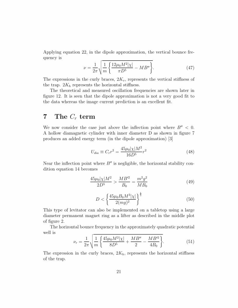
7 The Cr term

We now consider the case just above the inflection point where B′′ < 0.A hollow diamagnetic cylinder with inner diameter D as shown in figure 7produces an added energy term (in the dipole approximation) [3]

Udia ≡ Crr2 =

45µ0|χ|M2

16D5r2 (48)

Near the inflection point where B′′ is negligible, the horizontal stability con-dition equation 14 becomes

45µ0|χ|M2

2D5>MB′2

B0

=m2g2

MB0

(49)

D <

{45µ0B0M

3|χ|2(mg)2

} 15

(50)

This type of levitator can also be implemented on a tabletop using a largediameter permanent magnet ring as a lifter as described in the middle plotof figure 2.

The horizontal bounce frequency in the approximately quadratic potentialwell is

νr =1

2π

√√√√ 1

m

{45µ0M2|χ|

8D5+MB′′

2− MB

′2

4B0

}. (51)

The expression in the curly braces, 2Kh, represents the horizontal stiffnessof the trap.

21

����

��#�$

�% �&

' ('

���

$

��������!������� �)��*

�

�

$

�

�+�������� �

�� %�������� �

��

��

Figure 7: Vertical and horizontal stability curves for magnet levitation show-ing the stabilizing effect of a diamagnetic cylinder with an inner diameter of8 mm and the levitation geometry. Magnet levitation is stable where bothcurves are positive and the magnetic lifting force matches the weight of themagnet.

22

8 Counterintuitive levitation configuration

There is another remarkable but slightly counterintuitive stable levitationposition. It is above a lifter ring magnet with the floater in an attractiveorientation. Even though it is in attractive orientation, it is vertically stableand horizontally unstable. The gradient from the lifter repels the attractingmagnet but the field doesn’t exert a flipping torque. This configurationis a reminder that it is not the field direction but the field gradient thatdetermines whether a magnet will be attracted or repelled. A bismuth orgraphite cylinder can be used to stabilize the horizontal instability.

Figure 8 shows the stability functions and magnetic fields for this lev-itation position above the lifter magnet. We have confirmed this positionexperimentally.

9 Experimental results

Before we can compare the experimental results to the theory, we need toknow the values of the magnetic dipole moment of the magnets and thesusceptibility of diamagnetic materials we use. The dipole moment can bedetermined by measuring the 1/r3 fall of the magnetic field on axis far froma small magnet. For Nd2Fe14B magnet material, it is an excellent approxi-mation to consider the field as created by a solenoidal surface current anduse the finite solenoid equation (34) fit to measurements.

The diamagnetic susceptibility was harder to measure. Values in theHandbook of Chemistry and Physics were problematic. Most sources agreeon some key values such as water and bismuth. (There are multiple quantitiescalled susceptibility and one must be careful in comparing values. Physicistsuse what is sometimes referred to as the volume susceptibility. Chemists usethe volume susceptibility divided by the density. There is also a quantitysometimes called the gram molecular susceptibility which is the volume sus-ceptibility divided by the density and multiplied by the molecular weight ofthe material. There are also factors of 4π floating around these definitions.In this paper we use the dimensionless volume susceptibility in SI units).

The values given in the Handbook of Chemistry and Physics and othersome other published sources for graphite are inexplicably low. This couldbe because graphite rods have many different compositions and impurities.Iron is a major impurity in graphite and can overwhelm any diamagnetic

23

� � � � ��

�����

�����

�����

����

����

����

����

����

� � � � ��

��

��

�

�

��

��

��

������� ��

��

���

����� ��

Figure 8: top: Vertical and horizontal stability curves for magnet levitation adistance H above a ring lifter magnet. The dashed line shows the stabilizingeffect of a diamagnetic cylinder. Magnet levitation is stable where bothcurves are positive and the magnetic lifting force matches the weight of themagnet. bottom: B (T), B′ (T/cm), B′′ (T/cm2), and mg/M (T/cm) for a16 cm OD, 10 cm ID, 3 cm thick ring lifting magnet and a NdFeB floater.

24

effect. We have seen graphite rods that are diamagnetic on one end andparamagnetic on the other. Braunbek noticed that used graphite arc rodswere more diamagnetic on the side closest the arc. He speculated that thebinder used in the rods was paramagnetic and was vaporized by the heatof the arc. We found that in practice, purified graphite worked as well asbismuth and our measurements of its susceptibility were consistent with this.

Values for a form of graphite manufactured in a special way from thevapor state called pyrolytic graphite, are not given in the Handbook and theother literature gives a wide range of values. Pyrolytic graphite is the mostdiamagnetic solid substance known. It has an anisotropic susceptibility. Per-pendicular to the planar layers, the diamagnetic susceptibility is better thanin pure crystal graphite [21]. Parallel to the planar layers, the susceptibilityis lower than randomly oriented pressed graphite powder.

We developed a technique to measure the diamagnetic susceptibility ofthe materials we used. Later, we were able to get a collaborator (Fred Jeffers)with access to a state of the art vibrating sample magnetometer to measuresome samples. There was very good agreement between our measurementsand those made using the magnetometer.

9.1 Measurements of diamagnetic susceptibility

A simple and useful method for testing whether samples of graphite arediamagnetic or not (many have impurities that destroy the diamagnetism) isto hang a small NdFeB magnet, say 6 mm diameter as the bob of a pendulumwith about 1/2 m of thread. A diamagnetic graphite piece slowly pushedagainst the magnet will displace the pendulum a few cm before it touches,giving a quick qualitative indication of the diamagnetism.

The method we used to accurately measure the susceptibility was to hanga small NdFeB magnet as a pendulum from pairs of long threads so that themagnet could move along only one direction. The magnet was attached toone end of a short horizontal drinking straw. At the other end of the straw, asmall disk of aluminum was glued. A translation stage was first zeroed withrespect to the hanging magnet without the diamagnetic material present.Then the diamagnetic material to be tested was attached to a micrometertranslation stage and moved close to magnet, displacing the pendulum fromthe vertical. The force was determined by the displacement from vertical ofthe magnet and χ was determined from equations 39 and 17 which is plottedas the force in figure 6.

25

A sample of bismuth was used as a control and matched the value in thestandard references [22]. Once the value for our sample of bismuth was con-firmed, the displacement was measured for a fixed separation d between themagnet and bismuth. All other samples were then easily measured by usingthat same separation d; the relative force/translation giving the susceptibilityrelative to bismuth.

The difficult part was establishing a close fixed distance between the mag-net and the diamagnetic material surface with high accuracy. This problemwas solved by making the gap part of a sensitive LC resonant circuit. At-tached to the translation stage a fixed distance from the diamagnetic materialunder test, was the L part of the LC oscillator. When the gap between thediamagnet and magnet reached the desired fixed value, the flat piece of alu-minum on the other side of the straw from the magnet, came a fixed distancefrom the L coil, changing its inductance. The separation distance could beset by turning a micrometer screw to move the translation stage until thefrequency of the LC circuit reached the predetermined value for each sampleunder test. The setup is shown in figure 9.

This method was perhaps more accurate for our purposes than the vi-brating sample magnetometer, an expensive instrument. Our method wasindependent of the volume of the diamagnetic material. The vibrating sam-ple magnetometer is only as accurate as the volume of the sample is known.Samples are compared to a reference sample of nickel with a specific geometry.Our samples were not the same geometry and there was some uncertainty inthe volume. Our measurements measured the susceptibility of the materialin a way relevant to the way the material was being used in our experiments.

We measured various samples of regular graphite and pyrolytic graphiteand bismuth. Our average values for the graphite materials are shown intable 1 and are consistent with the values from the vibrating sample mag-netometer. Our value for graphite is higher than many older values such asthat reported in the Handbook of Chemistry and Physics, but is lower thanthat stated in a more recent reference [23]. Our values for pyrolytic graphiteare below the low end of the values stated in the literature [18, 24]. The valuefor the pyrolytic graphite parallel to the planar layers is from the vibratingsample magnetometer.

26

������������!����� ���

���� ����� ������ ��� �

��� ������ ��

������

�� ������

!� ,� ��������� �

���� �������

'� � ��� �����

Figure 9: Setup for measuring diamagnetic susceptibility. The diamagneticmaterial is moved close to the magnet, deflecting the magnet pendulum, untilthe gap between the magnet and diamagnet reaches a preset value. When thealuminum is a fixed distance from the inductor coil, the LC circuit resonatesat the desired frequency, corresponding to the preset value of the gap. Thisis an accurate way to measure the small gap. The force is determined fromthe displacement of the pendulum. The force is then compared to the forcefrom a previously calibrated sample of bismuth with the same gap.

27

9.2 Experimental realization of levitation

The fingertip and book stabilized levitation shown in figure 1 was achievedusing a 1 m diameter 11 T superconducting solenoid 2.5 m above the levitatedmagnet where the field was 500 G. Using regular graphite and an inexpensiveceramic lifter magnet it is possible to make a very stable levitator about 5 cmtall with a gap D of about 4.4 mm for a 3.175 mm thick 6.35 mm diameterNdFeB magnet. Using pyrolytic graphite, the gap D increases to almost 6mm for the same magnet. This simple design (similar to figure 4) could findwide application. The stability curves and gradient matching condition canbe seen in figure 10. The magnitude of Cz was determined from the forcegradient of figure 6 with L/R = 1 at two different gaps d using our measuredsusceptibility of pyrolytic graphite.

Figure 7 shows an experimental realization of horizontal stabilization atthe High Field Magnet Laboratory in Nijmegen. We also achieved horizontalstabilization on a tabletop using a permanent magnet ring and a graphitecylinder.

We were recently able to achieve stable levitation at the counterintuitiveposition above the ring lifter magnet (described above). The floater is inattractive orientation but is naturally vertically stable and radially unstable.Radial stabilization was provided by a hollow graphite cylinder.

Other configurations for diamagnetically stabilized magnet levitation arepossible and rotational symmetry is not required. For example, at the levi-tation position described just above, if an oval magnet or a noncircular arrayis used for a lifter instead of a circular magnet, the x− z plane can be madestable. Instead of using a hollow cylinder to stabilize the horizontal motion,flat plates can be used to stabilize the y direction motion.

For vertical stabilization with flat plates, if a long bar magnet is usedhorizontally as a lifter, the levitation point can be turned into a line. With aring magnet, the equilibrium point can be changed to a circle. Both of thesetricks have been demonstrated experimentally.

Another quite different configuration is between two vertical magnet polefaces as shown in figure 11. Between the pole faces, below center and justabove the inflection point in the magnetic field magnitude, the floating mag-net is naturally vertically stable. Diamagnetic plates then stabilize the hori-zontal motion. To our knowledge, this configuration was first demonstratedby S. Shtrikman.

28

� � �

��

��

�

�-%

-&

��

� � �

�����

�����

�����

����

����

����

����

����

��

�

�

�

�

������

�

Figure 10: top: Stability functions Kv and Kh for the demonstration levita-tor. Stability is possible where both functions are positive. The dashed linesshow the effect of two different values of the Cz term on Kv. The smallervalue corresponds to a large gap spacing d = 1.9 mm. The larger value cor-responds to a gap of only 0.16 mm. bottom: The levitation position is where−mg/M intersects the gradient −B′ at approximately H = 4.5 cm below thelifter magnet. B in T, −B′ in T/cm, and B′′ in T/cm2.

29

!

�

�"

#

$"

�"

#

Figure 11: Graphite plates stabilize levitation of a magnet below the center-line between two pole faces and just above the inflection point in the fieldmagnitude. Not shown in the picture but labelled N and S in the figure arethe 25 cm diameter pole faces of an electromagnet spaced about 15 cm apart.The poles can be from permanent or electromagnets.

30

9.3 Measurements of forces and oscillation frequencies

One way to probe the restoring forces of the diamagnetic levitator is tomeasure the oscillation frequency in the potential well. For the verticallystabilized levitator of figure 4 we measured the vertical oscillation frequencyas a function of the gap spacing d and compared it to the dipole and imagecurrent forces and prediction equations 46 and 47. The lifting magnet usedfor this experiment was a 10 cm long by 2.5 cm diameter cylindrical magnet.This magnet was used because its field could be accurately determined fromthe finite solenoid equation. The dipole moment was measured to be 25 Am2.The floater magnet was a 4.7 mm diameter by 1.6 mm thick NdFeB magnetwith a dipole moment of 0.024 Am2. It weighed 0.22 grams and levitated 8cm below the bottom of the lifter magnet as expected.

The graphite used was from a graphite rod, not pyrolytic graphite. Wemeasured this sample of graphite to have a susceptibility of −170×10−6. Theoscillation frequency was determined by driving an 1800 Ohm coil below thelevitated magnet with a sine wave. The resonant frequency was determinedvisually and the vibration amplitude kept small. The gap was changed bycarefully turning a 1

4–20 screw.

Figure 12 shows the theoretical predictions and the experimental mea-surements of the oscillation frequency as a function of gap spacing d. Thereare no adjustable parameters in the theory predictions. All quantities weremeasured in independent experiments. The agreement between the data andthe image current calculation is remarkably good. There is a limit to howmuch the total gap D = 2d + l can be increased. If D is too great, thepotential well becomes double humped and the magnet will end up closer toone plate than the other. The last point with d greater than 1.4 mm wasclearly in the double well region and was plotted as zero.

10 Levitation solutions for a cylindrically sym-

metric ring magnet

A ring magnet provides many combinations of fields, gradients and curvaturesas shown in figure 13. Considering the field topology but not the magnitudes,we show all possible positions where diamagnets, spin-stabilized magnets,and magnets stabilized by diamagnetic material can levitate. The fields andgradients shown may not be sufficient to levitate a diamagnet in the position

31

��� ��� ��� ��� � ��� ���

�

�

�

�

��

��

��

��%�&�

'�� ���� ��(�)���*�"

����� ������"�� ����� ���� �

Figure 12: Data points on the vertical oscillation frequency versus the gapspacing d with the dipole approximation prediction curve and the imagecurrent theory curve. The curves are not fit to the data. They are predictionsfrom the measured properties of the magnets and diamagnets, with no freeparameters. The last point is beyond the zero frequency limit and is plottedas zero. At zero frequency, the gap is too large to provide stability and thepotential well becomes double humped, with stable points closer to one platethan the other. This clearly was the case with the last point around d > 1.4mm.

32

Table 2: Magnetic field requirements for levitation of diamagnets, spin-stabilized magnet levitation, and diamagnetically stabilized levitation ofmagnets. + and – indicate the sign with respect to the sign of B.

M aligned with B B′ B′′

levit. of diamagnets – – + or –spin-stabilized magnet – – +diamag. stab. horiz. + + –diamag. stab. vert. + + +

Table 3: Stability functions for levitation of diamagnets, spin-stabilized mag-nets, and diamagnetically stabilized magnets. The functions must be positivefor stability and assume B0 in the positive z direction.

vertical horizontal

levit. of diamagnets B0B′′ +B′2 B′2 − 2B0B

′′

spin-stabilized magnet B′′ B′2 − 2B0B′′

diamag. stab. magnet Cz − 12MB′′ Cr +

14M

{B′′ − B′2

2B0

}

shown against 1 g of gravity, but the topology is correct if the magnetic fieldcould be increased enough.

Each type of levitation has its own requirements for radial and horizontalstability and the stable regions for each are shown. Other requirements suchas matching the magnetic field gradient to mg/M need be met. The fieldsmust be in the right direction so as not to flip the magnet. These requireddirections of B, B′, and B′′ are shown in table 2. The directions are allcompared to the direction of B.

The most fruitful place to look for levitation positions is around the inflec-tion points of the magnetic field. These are the places where the instability isweakest. The two levitation regions in figure 13 marked with a question markhave not been demonstrated experimentally and are probably not accessiblewith current magnetic and diamagnetic materials. The lower position witha question mark would work using a diamagnetic cylinder for radial stabi-lization. However, it may require more diamagnetism than is available. Thelevitation positions without the question marks have been demonstrated ex-perimentally. The position for levitation of a diamagnet marked with the *has been recently demonstrated by the authors.

33

�� ��� � �� �

�����

�����

�����

�����

����

����

����

����

��

��

����� � ���( �����. �

���� ��� �����.����

// +

�

�� �

�

��

Figure 13: B (T), B′ (T/cm), and B′′ (T/cm2), for a 16 cm OD, 10 cm ID, 3cm thick ring lifting magnet showing the fields on axis above and below themagnet. All possible levitation positions are shown for spin-stabilized mag-net levitation, diamagnetically stabilized magnet levitation, and levitationof diamagnets. h and v indicate use of diamagnetic material for horizontalor vertical stabilization. The two regions with question marks have not yetbeen verified experimentally and may be difficult to achieve. The levitationof diamagnets marked with * has recently been demonstrated by the authors.

34

The locations for diamagnetically stabilized magnet levitation are inter-esting for another reason. At these locations servo control can be used toprovide active stabilization very efficiently, since the instability is weak atthose locations. The diamagnetic plates or cylinder act as a very weak servosystem.

Acknowledgements

We acknowledge fruitful communications with Michael Berry. We would liketo thank Marvin Drandell for his help fabricating many prototype levitators,Rudy Suchannek for his translation of Braunbek’s [10] papers from German,and Fred Jeffers for helping confirm our susceptibility measurements.

35

References

[1] M. V. Berry and A. K. Geim, “Of flying frogs and levit-rons”, Euro. J. Phys., 18, 307–313 (1997) and http://www-hfml.sci.kun.nl/hfml/levitate.html.

[2] A. Geim, “Everyone’s Magnetism”, Phys. Today, 51 Sept., 36–39 (1998).

[3] A. K. Geim, M. D. Simon, M. I. Boamfa, L. O. Heflinger, “Magnet levi-tation at your fingertips”, Nature, 400, 323–324 (1999).

[4] M. D. Simon and A. K. Geim, “Diamagnetic levitation; Flying frogs andfloating magnets”, J. App. Phys., 87, 6200–6204 (2000).

[5] N. W. Ashcroft and N. D. Mermin, Solid State Physics, ch. 31, 647,Harcourt Brace, New York, (1976).

[6] R. P. Feynman, R. B. Leighton, and M. Sands, The Feynman Lecturesin Physics, vol. II, chp. 34 sec. 6, Addison-Wesley Publishing Company,New York (1963).

[7] S. Earnshaw, “On the nature of the molecular forces which regulate theconstitution of the luminiferous ether”, Trans. Camb. Phil. Soc., 7, 97-112 (1842).

[8] K. T. McDonald, “Laser tweezers”, Am. J. Phys., 68, 486–488 (2000).

[9] W. Thomson, “Reprint of Papers on electrostatics and magnetism”,XXXIII, 493-499, and XXXIV, 514-515, London, MacMillan (1872).

[10] W. Braunbek, “Freischwebende Korper im elecktrischen und magnetis-chen Feld” and “Freies Schweben diamagnetischer Korper im Magnetfeld”Z. Phys., 112, 753–763 and 764–769 (1939).

[11] V. Arkadiev, “A floating magnet”, Nature, 160, 330 (1947).

[12] R. M. Harrigan, U.S. patent 4,382,245, (1983).

[13] M. D. Simon, L. O. Heflinger, and S. L. Ridgway, “Spin stabilized mag-netic levitation”, Am. J. Phys., 65, 286–292 (1997).

[14] M. V. Berry, “The LevitronTM : an adiabatic trap for spins”, Proc. Roy.Soc. Lond. A, 452, 1207–1220 (1996).

36

[15] Personal communication with Ed Phillips.

[16] V. V. Vladimirskii, “Magnetic mirrors, channels and bottles for coldneutrons”, Sov. Phys. JETP,12,740-746 (1961) and W. Paul, “Electro-magnetic traps for charged and neutral particles”, Rev. Mod. Phys., 62,531-540 (1990).

[17] A. H. Boerdijk, “Technical aspects of levitation”, Philips Res. Rep., 11,45–56 (1956) and A. H. Boerdijk, “Levitation by static magnetic fields”,Philips Tech. Rev., 18, 125–127 (1956/57).

[18] V. M. Ponizovskii, “Diamagnetic suspension and its applications (sur-vey)”, Prib. Tek. Eksper., 4, 7–14 (1981).

[19] W. R. Smythe, Static and Dynamic Electricity, Hemisphere PublishingCorporation, New York, third ed., (1989).

[20] M. V. Berry first suggested the simplification of treating the lifter mag-net as a dipole and derived equation 33 in a 1997 correspondence withM. D. Simon.

[21] D. B. Fischback, “The magnetic susceptibility of pyrolytic carbons”,Proceedings of the Fifth Conference on Carbon, 2, 27–36,(1963).

[22] For example, the Handbook of Chemistry and Physics, The ChemicalRubber Co.

[23] I. Simon, A. G. Emslie, P. F. Strong, and R. K. McConnell, Jr., “Sensi-tive tiltmeter utilizing a diamagnetic suspension”, The Review of Scien-tific Instruments, 39, 1666–1671, (1968).

[24] R. D. Waldron, “Diamagnetic levitation using pyrolytic graphite”, TheReview of Scientific Instruments, 37, 29–35, (1966).

37