Dialectometry

Wilbert Heeringa and John Nerbonne

1. Introduction

We discuss quantitative work on Dutch dialectology, a line of work that is often referred to as

‘dialectometry’. It is worth emphasizing that a great deal of both the Dutch dialectometric work and

also work on other languages and dialects has been inspired by the wish to overcome problems in

the traditional methodology of dialectology, which has focused on the geographic distributions of

single linguistic features (Nerbonne 2009). Examples are two isogloss maps of Weijnen which were

published in 1941 (based on 45 isoglosses) and 1958 (based on another set of 18 isoglosses) and the

isogloss map of Goossens which appeared in 1970. The three maps suggest different classifications

since the choice of the isoglosses differs per map. Isogloss maps are verifiable, but the motivation

for the selection of the isoglosses remains unclear. Goossens (1977) mentioned that the isogloss

method cannot be applied without making subjective choices. The dialectometric strategy has been

to seek more satisfying characterizations by aggregating over large number of linguistic features.

The aggregating step is inevitably quantitative, which has allowed the introduction of powerful

quantitative techniques into dialectology.

2. Literature survey

2.1. Categorical measurements: Background

Séguy

The first to develop a method of measuring dialect distances was Jean Séguy, assisted and inspired

by Henri Guiter. Jean Séguy was director of the Atlas linguistique de la Gascogne. He and his

associates published six atlas volumes containing maps in which single responses were plotted for

154 dialect locations. Séguy’s major survey used five types of linguistic variables: 67 features from

diachronic phonetics, 76 from phonology, 68 from morphosyntax, 44 from verb morphology and

170 lexical items, 425 variables in total. Séguy sought a way to analyse the maps in a more

satisfying way than was possible with traditional analytic methods, and came up with the idea of

counting “the number of items on which neighbors disagreed.” (Chambers and Trudgill 1998: 138).

At the back of the sixth volume of the atlas, a map is provided for each of the linguistic levels in

which the number of items on which two neighboring dialect locations disagree is printed between

the two dialect locations. After these six maps, there are two additional maps in which the six maps

are aggregated. On the second map, the total number of disagreements between two neighbors was

expressed as a percentage: the number of agreements divided by 425 times 100. The percentage

“was treated as an index score indicating the linguistic distance between any two places” (Chambers

and Trudgill 1998: 138, see also Séguy 1973a, 1973b, 1973c).

Goebl

Hans Goebl continued and elaborated on Séguy’s work, striking out independently in several

respects. We base our sketch on Goebl (1982a, 1984, 1993). Goebl most extensively analysed

l'Atlas Linguistique de l'Italie et de la Suisse Méridionale (AIS), compiled by Karl Jaberg and Jakob

Jud in the first quarter of the twentieth century. He selected 251 varieties and 696 working maps

from the AIS. Each working map represents a dialect feature and requires assigning a value at each

of the 251 sites. 569 maps represent lexical variation, and 127 maps represent morphosyntactic

variation. While Séguy calculated distances, Goebl calculated similarities. The similarity between

two varieties is calculated as the percentage of items on which the two varieties agree. Goebl refers

to this measure as ‘relative similarity’ (originally in German: relativer Identitätswert, RIW). He

also introduced a second measure: weighted similarity (originally: gewichteter Identitätswert,

GIW). The GIW method weights infrequent feature overlap among pairs of dialect varieties in a

dialect area more heavily than frequent feature similarities, opposing the tendency in several areas

of quantitative linguistics that very infrequent words should be treated as noise, unreliable evidence

of linguistic structure (Nerbonne and Kleiweg 2007). Features which are common to few dialects,

but which are found only infrequently overall, characterize the dialects’ similarity more strongly

than features which are also found in many dialects. For this reason similarity between dialects

depends more on infrequently shared features than on frequently occurring features.

Goebl also introduced THIESSEN tiling to dialectology, a technique which draws tiles around

points on a map so that maps are divided into regions around sampling sites as evenly as possible.

This technique produces the basis of CHLOROPLETH maps, in which each of the tiles is assigned a

linguistic value based on (similarity) calculations with respect to a reference point, e.g. a single

village. Goebl’s work examines a large range of descriptive statistics derived from the distribution

of linguistic similarity, and he examines each of these, e.g. similarity with respect to the entire

range of reference sites. It is quite characteristic of Goebl’s work that he insists on examining

variation from each of a large range of locations, e.g. Paris, Lyon, etc. when the AIS is analyzed.

Goebl (1993) also uses INTERPOINT maps which depict distances between neighboring dialects as

“walls” which grow in darkness as the linguistic dissimilarity increases. This visualization is also

called the HONEYCOMB method (Inoue 1996). A complementary visualization technique is the BEAM

MAP, also used by Séguy. Linguistically similar dialects are connected by dark beams, and more

dissimilar ones by lighter beams (see Figure 1a). On the basis of distances among dialect varieties

Goebl performs cluster analysis (Goebl 1982b, 1983), thus finding the main dialect groups which

are geographically shown as differently colored dialect areas in a map.

2.2. Application to Frisian and Dutch

Séguy and Goebl’s methodology has also been applied to Frisian and Dutch varieties at the lexical,

phonological, morphological and syntactic level. The variables used in this methodology are usually

nominal.1 On the basis of these variables, the number (or percentage) of agreements (similarity) or

disagreements (distance) are measured, and these measurements are numerical.2 In the studies we

mention below in this section, the measurements are numerical.

Lexicon

Kruijssen (1990,1992) presented a study aimed at determining whether the dialect of Lommel,

regarded as a Brabant dialect, actually belonged to the Limburg group. He measured the lexical

similarities between Lommel and a set of 12 Limburg varieties à la Séguy and Goebl using data

from the Woordenboek of Limburgse Dialecten (‘Dictionary of Limburg Dialects’, Weijnen and

Goossens (1983-2008)). Kruijsen found that the distance between Lommel and the closest Limburg

dialect was nearly as large as the largest distance within the Limburg group. It is therefore not likely

that Lommel is a Limburg variety.

Heeringa and Nerbonne (2006) measured lexical distances among 360 varieties in the Dutch

dialect area. This area comprises the Netherlands, the northern part of Belgium and French

Flanders. The measurements are based on 125 items taken from the Reeks Nederlandse

Dialectatlassen (RND, Blancquaert and Pée (1925-1982)). Lexical distances were measured using

Goebl's GIW. They found that the varieties are lexically divided into Frisian varieties (including

Frisian mixed varieties), Low Saxon varieties, Holland varieties (including Zeeland, Utrecht and the

Veluwe), and southern Dutch varieties (Flemish, Brabant, Limburg). The latter group is a

geographically large area, but in the same paper the authors show that this area is divided into even

smaller groups at the level of the sound components.

Giesbers (2008) measured lexical distances between 10 locations in the Kleverlands area,

1 That is, the values which a nominal variable may have are like names. When comparing values of a nominal variable,

they are either equal or different, and we cannot measure the degree to which values differ. 2 Or: ratio measurements, i.e. measurements are numbers on a scale which has an absolute zero.

along the Dutch-German national border. She selected five bi-national pairs of sites and measured

distances among the pairs of varieties and with respect to standard Dutch and German. Since

Giesbers also measures pronunciation distances, we return to this study in Section 2.3.3.

Pronunciation

Klaas van der Veen, following the work of Séguy and Goebl (van der Veen 1986; van der Veen

1994), measured similarity among West Lauwers Frisian varieties on the basis of word isoglosses.

For example, the Frisian word forms of niet ‘not’ are net and nit, dividing the Frisian varieties into

two groups. The Frisian forms of recht ‘straight’ are rjocht, rjucht and rucht, dividing the Frisian

varieties into three groups. In van der Veen (1986), 87 word isoglosses are listed, and in van der

Veen (1994) we count 96 word isoglosses. The words chosen are the most highly frequent words in

written West Lauwers Frisian, and the pronunciations are gathered from different sources (e.g. the

RND). In contrast to Séguy and Goebl, van der Veen weights isoglosses directly by the relative

frequencies of the words in which they occur. Like Goebl, he uses cluster analysis to identify

groups among the varieties.

Morphology

Heeringa et al. (2009) focus on morphological distances as measured among Low Saxon varieties.

Séguy’s overlap measure is applied to data from the Morphological Atlas of Dutch Dialects (De

Schutter et al. 2005, Goeman et al. 2009). The following feature domains are considered: plural

substantives (43 features), diminutives (39 features), possessive pronouns (11 features), verbs

(present tense and past tense, 24 features), participle prefix GE- (4 features) and verb stem

alternations (past tense, 16 features). The distance measurements corresponding with the domains

are weighted equally and aggregated. They determine four groups: 1) Groningen, 2) the northern

part of Drenthe, 3) Stellingwerven, Kop van Overijssel and Salland, 4) Achterhoek and Twente.

Syntax

Spruit (2008) measured syntactic distances among 267 varieties in the Dutch dialect area. He used

data from the Syntactic Atlas of Dutch Dialects (Barbiers, Bennis and De Vogelaer 2004) and

applied Goebl’s RIW and GIW. GIW resulted in more sharply distinguished groups than RIW (see

also Spruit, Heeringa and Nerbonne 2009). Spruit shows a dominant split between a northern group

(including Frisian, Holland and Low Saxon varieties) and a southern group. Within the southern

group the West Flemish varieties and the Limburg varieties are clearly distinguished.

2.3. Frequency-based methods

2.3.1. Profile-based linguistic uniformity

Profile-based linguistic uniformity compares language varieties on a range of heterogeneous

linguistic variables in corpora created for this purpose and was introduced by Geeraerts,

Grondelaers and Speelman (1999), who used it to study register variation and regional variation in

Dutch. Their aim was to see whether Belgian and Netherlandic Dutch converged from 1950 to 1990

and whether the convergence was due to Belgian changes. Focusing on the lexicon, they assume

formal onomasiological variation occurs when different terms are used to refer to the same entity.

They define a formal onomasiological profile, or profile: “a profile for a particular concept […] is

the set of alternative linguistic means used to designate that concept or linguistic function in that

variety, together with their frequencies (expressed as relative frequencies, absolute frequencies or

both).”

For example the concept jeans appears in their Netherlands sample 81 times (70%) as jeans

and 34 times (30%) as spijkerbroek. In Belgium, the frequencies are 64 (97%) and 2 (3%)

respectively. The distance between the two profiles is the sum of the absolute differences between

the corresponding relative frequencies:3 (|70-97]) + (|30-2|) =55%. The distance between two

varieties is usually based on several concepts and is calculated as the sum of the corresponding

profile distances. The concepts need not be lexical, but may be morphological or syntactic as well.

Once distances are calculated, statistics can be applied to classify the varieties. Speelman,

Grondelaers and Geeraerts (2003) apply multidimensional scaling, which we discuss below in

Section 3.2.

2.3.2. Phone and feature frequency methods

Hoppenbrouwers and Hoppenbrouwers developed the phone frequency method (PFM) and the

feature frequency method (FFM) to measure dialect distances on the basis of pronunciation. The

methods were introduced in 1988 and also described by Hoppenbrouwers and Hoppenbrouwers

(2001). An extended analysis of their work is given by Heeringa (2002).

Phone frequency method

Hoppenbrouwers and Hoppenbrouwers (2001: 1) suggest comparing varieties based on samples of

speech in phonetic transcription. They count the frequencies of phones (segments) in each sample.

Since samples differ in size, relative frequencies are used. The distance between varieties is the sum

of the absolute values of the differences between their (relative) phone frequencies. We illustrate

this in an small example. Let us assume for two dialects A and B the following relative frequencies

in their samples:

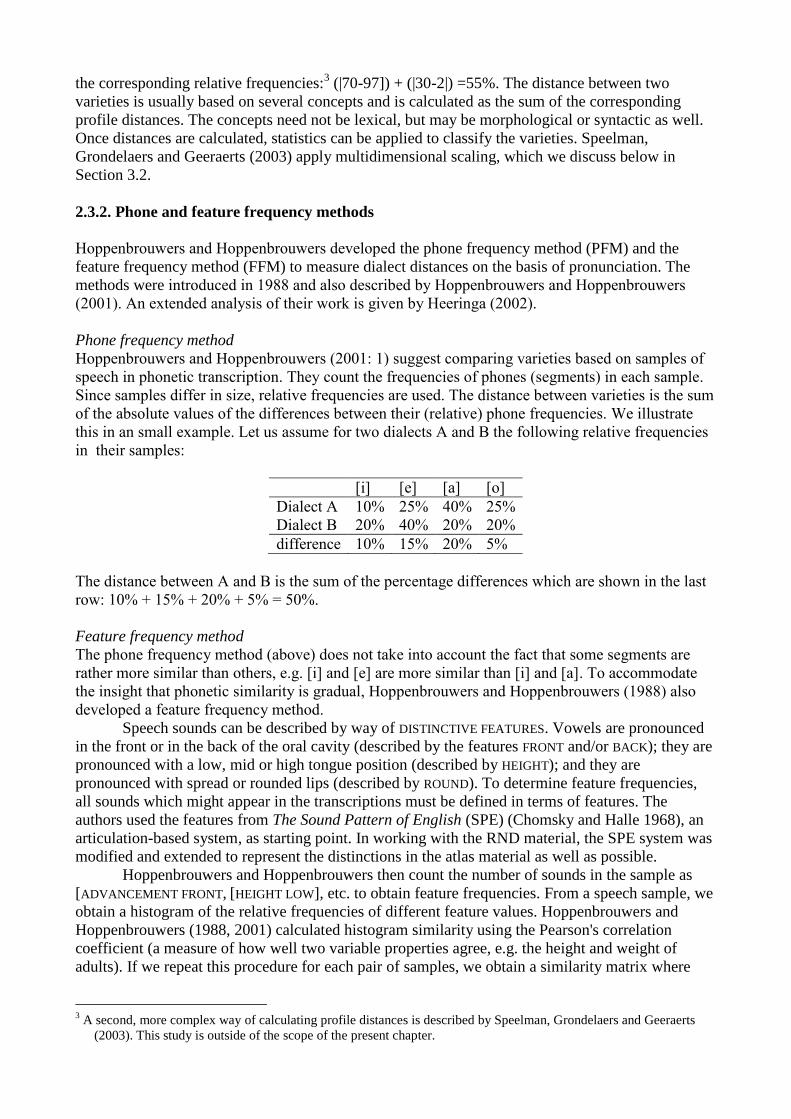
[i] [e] [a] [o]

Dialect A 10% 25% 40% 25%

Dialect B 20% 40% 20% 20%

difference 10% 15% 20% 5%

The distance between A and B is the sum of the percentage differences which are shown in the last

row: 10% + 15% + 20% + 5% = 50%.

Feature frequency method

The phone frequency method (above) does not take into account the fact that some segments are

rather more similar than others, e.g. [i] and [e] are more similar than [i] and [a]. To accommodate

the insight that phonetic similarity is gradual, Hoppenbrouwers and Hoppenbrouwers (1988) also

developed a feature frequency method.

Speech sounds can be described by way of DISTINCTIVE FEATURES. Vowels are pronounced

in the front or in the back of the oral cavity (described by the features FRONT and/or BACK); they are

pronounced with a low, mid or high tongue position (described by HEIGHT); and they are

pronounced with spread or rounded lips (described by ROUND). To determine feature frequencies,

all sounds which might appear in the transcriptions must be defined in terms of features. The

authors used the features from The Sound Pattern of English (SPE) (Chomsky and Halle 1968), an

articulation-based system, as starting point. In working with the RND material, the SPE system was

modified and extended to represent the distinctions in the atlas material as well as possible.

Hoppenbrouwers and Hoppenbrouwers then count the number of sounds in the sample as

[ADVANCEMENT FRONT, [HEIGHT LOW], etc. to obtain feature frequencies. From a speech sample, we

obtain a histogram of the relative frequencies of different feature values. Hoppenbrouwers and

Hoppenbrouwers (1988, 2001) calculated histogram similarity using the Pearson's correlation

coefficient (a measure of how well two variable properties agree, e.g. the height and weight of

adults). If we repeat this procedure for each pair of samples, we obtain a similarity matrix where

3 A second, more complex way of calculating profile distances is described by Speelman, Grondelaers and Geeraerts

(2003). This study is outside of the scope of the present chapter.

each variety is defined as a vector (row) of similarity values with respect to all other varieties (and

to itself). Cluster analysis was applied to the similarity matrix to find groups (areas).

2.3.3. Application to Dutch

Hoppenbrouwers and Hoppenbrouwers (2001) is the most extensive application of the feature

frequency method. The authors work with full RND texts, each containing 139 sentences

transcribed phonetically. Using 156 varieties, they find a main division into Low Saxon, Limburg

and other varieties. The other varieties consist of three subgroups: 1) Frisian (including Town

Frisian, Het Bildt and Stellingwerf varieties), 2) Holland and North-Brabant, 3) Zeeland, Flemish

and Belgian Brabant.

They also measured distances between dialect varieties and standard Dutch, finding the

Limburg and Groningen varieties most distant, and those in North-Holland, South-Holland and

Utrecht closest. Surprisingly, the Frisian varieties were measured to be relatively close to standard

Dutch. We will return to this in Section 3.2. See Heeringa, Nerbonne and Osenova (2010) for an

application of Hoppenbrouwers’ techniques in contact linguistics which exploit the advantage of

these techniques in that they do not require the same words to be sampled in different sites.

3. Recent work: Techniques using edit distance

A disadvantage of the frequency-based methods is that they are not sensitive to the order of

phonetic segments in a word. For example, the word konijn ‘rabbit’ is pronounced as [] in the

dialect of Deelen and as [] in the dialect of De Lutte. The two pronunciations will erroneously

be considered as identical in frequency-based techniques. Séguy and Goebl would examine each

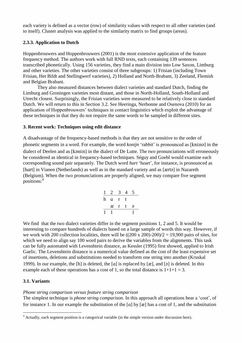
corresponding sound pair separately. The Dutch word hart ‘heart’, for instance, is pronounced as

[] in Vianen (Netherlands) as well as in the standard variety and as [] in Nazareth

(Belgium). When the two pronunciations are properly aligned, we may compare five segment

positions:4

1 2 3 4 5

1 1 1

We find that the two dialect varieties differ in the segment positions 1, 2 and 5. It would be

interesting to compare hundreds of dialects based on a large sample of words this way. However, if

we work with 200 collection localities, there will be ((200 x 200)-200)/2 = 19,900 pairs of sites, for

which we need to align say 100 word pairs to derive the variables from the alignments. This task

can be fully automated with Levenshtein distance, as Kessler (1995) first showed, applied to Irish

Gaelic. The Levenshtein distance is a numerical value defined as the cost of the least expensive set

of insertions, deletions and substitutions needed to transform one string into another (Kruskal

1999). In our example, the [] is deleted, the [] is replaced by [], and [] is deleted. In this

example each of these operations has a cost of 1, so the total distance is 1+1+1 = 3.

3.1. Variants

Phone string comparison versus feature string comparison

The simplest technique is phone string comparison. In this approach all operations bear a ‘cost’, of

for instance 1. In our example the substitution of the [] by [] has a cost of 1, and the substitution

4 Actually, each segment position is a categorical variable (in the simple version under discussion here).

of the [] by [] would cost the same, since the phonetic affinity between phones is ignored. A more

sensitive technique might use gradual distances between segments as operation weights, perhaps

calculating the weights on the basis of segmental features. When for example vowels are described

by three features (height, backness and roundness), distances between vowels can be calculated in

three-dimensional space and then used as operation weights in the Levenshtein distance, so that the

substitution of [] by [] will cost less than the substitution of [] by []. Kessler calls this metric

feature string comparison. Heeringa (2004) measures segment distances on the basis of several

feature systems, including the system implied by the IPA table organizing sounds by place and

manner of articulation and voicing (see also Heeringa and Braun 2003, who provide details). He

also measures distances between segments on the basis of their spectrograms. Since a spectrogram

is the curve plotting intensity against time and frequency, the curve distances between the

spectrograms reflect acoustic differences. The samples which the spectrograms are based on were

pronounced by John Wells and Jill House and are found in the recording The Sounds of the

International Phonetic Alphabet (1995).5 Heeringa (2004) focuses especially on the more

perceptually oriented models, which emphasize the differences that a speaker can hear in someone

else’s speech.

The choice of operation weights depends on one’s research goal. If the goal is to approximate how

differences are perceived by dialect speakers, then the use of binary costs (0/1) outperforms that of

gradual costs (Heeringa 2004), which suggests that the fact that segments differ is more important

than the degree to which they differ, perhaps reflecting the categorical basis of speech distinction.

All segmental weighting schemes to-date have led to only small differences in measurements at the

aggregate varietal level (Heeringa 2004: 186), giving only slightly different correlations to distances

as perceived by the dialect speakers themselves in a perception experiment. It is probably necessary

to validate measurements on individual words if we are to make progress in this area.

Free alignment versus forced alignment

To deal with syllabicity, the Levenshtein algorithm may be adapted so that only vowels may match

with vowels, and consonants with consonants, with several exceptions: [j] and [w] may match with

both consonants and vowels, [i] and [u] with both vowels and consonants, and central vowels

(which in our research boils down to schwa) with both vowels and sonorant consonants. So the [], [], [] and [] align with anything, the [] with syllabic (sonorant) consonants, but otherwise

vowels align with vowels and consonants with consonants. In this way unlikely matches (e.g., a [p]

with an [a]) are prevented. This approach was first applied to Sardinian dialects (Bolognesi and

Heeringa 2002), and then to Dutch (Heeringa and Braun, 2003). In a validation study, Heeringa et

al. (2006) found that forced alignments perform better than free alignments, i.e. they approach

dialect perception more closely.

Relative distances versus absolute distances

Nerbonne et al. (1996) normalized Levenshtein distances by dividing the absolute distance by the

length of the longer word, calling this relative edit distance. The idea behind this is to emphasize

the perception of words as crucial linguistic units. In the example with the two variants of the word

for ‘heart’, where we found a Levenshtein distance of 3, the relative distance would be 3/4= 0.75.

If a dialect variant consisting of five segments were included, the denominator value would be 5.

One may also choose to normalize using the sum of the lengths of the two variants (in our example:

4+4=8) or using the length of the cost alignment (in our example: 5). The different ways of

normalizing are discussed by Heeringa (2004: 130-132).

Again the choice between relative distances and absolute distances may depend on one’s

scientific goal. Heeringa et al. (2006) showed that absolute Levenshtein distances approximate

dialect differences as perceived by the dialect speakers better than results based on relative

Levenshtein distances, i.e. normalized by alignment length. This suggests that the weight of the

5 See http://www.phon.ucl.ac.uk/home/wells/cassette.htm.

substitution of e.g. the [u] in a word variant of dialect A by the [y] in the variant of the same word

in dialect B is independent of the length of the variant in the perception of the speakers. On the

other hand Beijering, Gooskens and Heeringa (2008) found that intelligibility correlates better with

relative distances than with absolute distances. In both cases the differences were not large.

All-word comparison vs. same-word comparison

Kessler calculated edit distances not only for words that are phonetic variants of each other, but also

for lexical variants, calling this the all-word approach. We can alternatively restrict our comparison

to words that are phonetic or phonological variants of each other, i.e. cognates, adopting Kessler’s

same-word approach. Both approaches have been applied to the same set of 360 Dutch dialects (see

also Section 3.2). The all-word approach is found in Heeringa (2004), and the same-word approach

is found in Heeringa and Nerbonne (2006). Although we did not publish the correlation between

both measures, it was in fact extremely high (r=0.99). The maps in the papers naturally coincide.

The classification map obtained on the basis of all-word distances shows 13 groups, and the

classification map obtained on the basis of same-word distances shows 11 groups. The maps are not

identical, but all borders in the same-word map are also found in the all-word map. The maps thus

do not contradict each other. This leads us to conjecture that non-cognate comparisons just act as

noise, but details may naturally differ in other data collections.

3.2. Application of Edit Distance to Frisian and Dutch

Measuring mutual relationships

Levenshtein distance was first applied to the comparison of Dutch dialect varieties by Nerbonne et

al. (1996). It was applied to 20 Dutch varieties, taken from the RND, where 100 word

pronunciations were digitized for each variety. All-word distances were calculated, and on the basis

of these distances the varieties were classified using cluster analysis. Cluster analysis had also been

used in the earlier Dutch dialectometric studies of van der Veen (1986, 1994). The goal is to

identify the main groups, or clusters. In hierarchical clustering, clusters may consist of subclusters,

and subclusters may in turn consist of subsubclusters, etc. The result is a hierarchically structured

tree in which the dialects are the leaves. Jain and Dubes (1988) mentioned seven alternative

clustering techniques. Nerbonne et al. (1996) used the Ward’s method, which gives a well-balanced

tree. Heeringa (2004: 150-153) found that Ward’s method yielded counterintuitive results and

found the Unweighted Pair Group Method using Arithmetic averages (UPGMA) superior.

Dendrograms naturally give rise to a “derived distance” between varieties, namely the distance over

the branches of the dendrogram. Heeringa and Nerbonne (2006) suggest that UPGMA derived

distances correlate most strongly with the original measurements, i.e. the measurements the cluster

technique was applied to. Nerbonne et al. (2008) investigate means of ensuring stability in

clustering as well. By ‘stability’ we mean the extent to which the clustering remains the same when

elements are modified in small ways.

We illustrate cluster analysis by a small example. Assume linguistic distances among five

Dutch dialects are measured, where the distances represent the average percentage to which dialect

pairs disagree at the level of the sound components, measured with Levenshtein distance. The

distances are arranged in the following table:

Grouw Haarlem Delft Hattem Lochem

Grouw 42 44 46 47

Haarlem 16 36 38

Delft 38 40

Hattem 21

Lochem

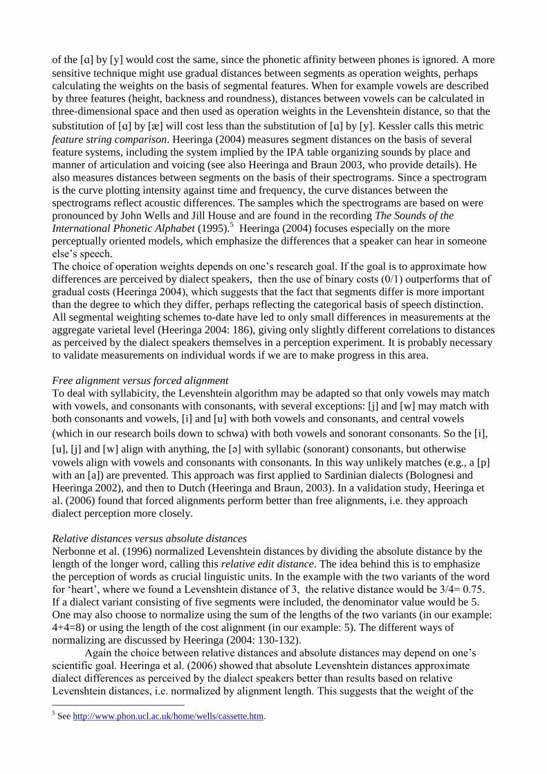
When we apply UPGMA cluster analysis to this table, we will obtain the following dendrogram:

Nerbonne and Heeringa (1998) published a study in which 104 varieties are involved and

100 word pronunciations for each variety. The data was taken from the RND, and all-word

pronunciation distances were measured. The distances are geographically shown in a beam map.

This type of map was introduced by Séguy (1973) and used by Goebl (1993) (see Section 2.1.1

above). Linguistically close varieties are connected by darker lines, and distant varieties are

connected by lighter ones.

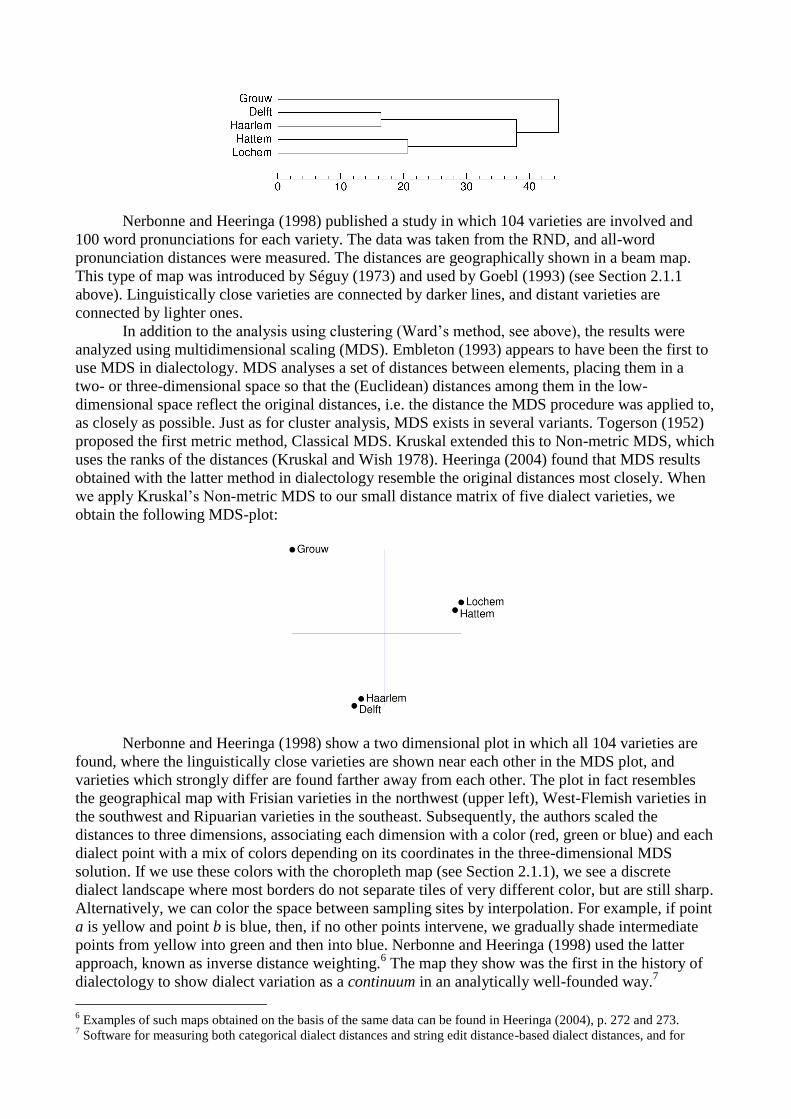
In addition to the analysis using clustering (Ward’s method, see above), the results were

analyzed using multidimensional scaling (MDS). Embleton (1993) appears to have been the first to

use MDS in dialectology. MDS analyses a set of distances between elements, placing them in a

two- or three-dimensional space so that the (Euclidean) distances among them in the low-

dimensional space reflect the original distances, i.e. the distance the MDS procedure was applied to,

as closely as possible. Just as for cluster analysis, MDS exists in several variants. Togerson (1952)

proposed the first metric method, Classical MDS. Kruskal extended this to Non-metric MDS, which

uses the ranks of the distances (Kruskal and Wish 1978). Heeringa (2004) found that MDS results

obtained with the latter method in dialectology resemble the original distances most closely. When

we apply Kruskal’s Non-metric MDS to our small distance matrix of five dialect varieties, we

obtain the following MDS-plot:

Nerbonne and Heeringa (1998) show a two dimensional plot in which all 104 varieties are

found, where the linguistically close varieties are shown near each other in the MDS plot, and

varieties which strongly differ are found farther away from each other. The plot in fact resembles

the geographical map with Frisian varieties in the northwest (upper left), West-Flemish varieties in

the southwest and Ripuarian varieties in the southeast. Subsequently, the authors scaled the

distances to three dimensions, associating each dimension with a color (red, green or blue) and each

dialect point with a mix of colors depending on its coordinates in the three-dimensional MDS

solution. If we use these colors with the choropleth map (see Section 2.1.1), we see a discrete

dialect landscape where most borders do not separate tiles of very different color, but are still sharp.

Alternatively, we can color the space between sampling sites by interpolation. For example, if point

a is yellow and point b is blue, then, if no other points intervene, we gradually shade intermediate

points from yellow into green and then into blue. Nerbonne and Heeringa (1998) used the latter

approach, known as inverse distance weighting.6 The map they show was the first in the history of

dialectology to show dialect variation as a continuum in an analytically well-founded way.7

6 Examples of such maps obtained on the basis of the same data can be found in Heeringa (2004), p. 272 and 273.

7 Software for measuring both categorical dialect distances and string edit distance-based dialect distances, and for

The most extensive Dutch study based on material of the RND was performed by Heeringa

(2004). All-word pronunciation distances among 360 different dialect varieties were involved, and

125 word pronunciations per variety were used. Cluster analysis was also applied. From the

dendrogram, a binary hierarchically structured tree, the main 13 clusters were examined, each of

them discussed in detail.8 A beam map, showing the 13 main groups found with cluster analysis,

and MDS continuum maps are included. Heeringa and Nerbonne (2006) use the same data set, but

measure same-word distances. A beam map and a choropleth MDS map obtained on the basis of the

measurements in this study are shown in Figures 1a and 1b. As noted in Section 3.1, results of the

all-word vs. same-word approaches are quite similar. The more global classification of the second

study shows a division into Frisian, Low Saxon, a large central group (Holland, Utrecht, North-

Brabant), West-Flemish (including Zeeland), East-Flemish, Flemish Brabant (including Antwerp),

and Limburg, which is divided into eastern and western groups and a small northern part of the

province of Liege. This classification partly agrees and partly disagrees with the classification

shown in the map of Daan and Blok (1969), which is the most recent Dutch dialect map.

Differences may be explained by the fact that the dialectometric map is obtained exclusively on the

basis of pronunciation while the map of Daan and Blok is obtained on the basis of the perception of

the speakers (Netherlandic part) and on the opinions of dialect speaking linguists (Belgian part).

In 2007 a study was published in which Wieling, Heeringa and Nerbonne measured same-

word pronunciation distances among 613 Dutch varieties, using data from the Goeman-Taeldeman-

van Reenen Project (GTRP)9 which was collected in the period 1980-1995. Since the Netherlandic

transcriptions are narrower than the Belgium ones, results are analyzed per country. Beam maps and

MDS continuum maps are shown. The maps suggest a classification which is quite similar to the

classification obtained on the basis of the RND measurements. The RND data set used in the studies

mentioned above and the GTRP data set have 224 localities and 59 words in common. The RND

and GTRP distances correlate strongly (r =0.83 in Netherlands, and r = 0.82 in Flanders).

Measuring with respect to a reference point

Besides measuring relationships among dialect varieties, it is useful to measure distances with

respect to a single reference point. For Dutch we find three examples: distance measurements

compared to Proto-Germanic, standard Dutch and Afrikaans.

Heeringa and Joseph (2007) measured same-word pronunciation distances between 360

Dutch dialect varieties and proto-Germanic. The same RND data set was used as in earlier studies,

and the proto-Germanic forms were taken from a proto-Germanic dictionary (Köbler, 2003). The

authors found that present-day Frisian varieties and the varieties in the eastern part of North-

Brabant are closest to proto-Germanic, while the Ripuarian varieties are most distant from proto-

Germanic.

Heeringa (2004) measured all-word distances between the set of 360 RND varieties and

standard Dutch. Each dialect variety is compared to standard Dutch by comparing 125 word

realizations to the corresponding standard Dutch pronunciations. The results were projected on a

map using colors according to the “rainbow” scheme: the closest varieties are red, while the most

distant varieties are blue. Intermediate points were colored using interpolation, just as in Nerbonne

and Heeringa’s (1998) MDS continuum map. The map is shown in Figure 1c. Frisian and Ripuarian

are most distant groups from standard Dutch, andthe dialect of Schiermonnikoog is the variety least

like standard Dutch. Closest are the Randstad varieties, where Haarlem is maximally close to

standard Dutch. Recall that Hoppenbrouwers and Hoppenbrouwers (2001) found that Groningen

creating all the types of maps mentioned in this contribution is included in Gabmap, a web application for

dialectometry developed at the University of Groningen and made freely available at: http://www.gabmap.nl/

(Nerbonne et al. 2011). 8 However, one group, the former island of Urk, contains only one variety and therefore does not branch.

9 For practical reasons Dutch dialectometrists used RND data for a long time. This does not mean that they judge the

RND data superior to the GTRP data. The GTRP data is collected in a much smaller time span and transcriber

differences may be smaller. Therefore, more recent analyses are based on the GTRP data.

and Limburg varieties were most distant and Frisian was relatively close to standard Dutch (see

Section 2.2.3). As explained in Section 2.3.1, frequency-based methods do not consider the

sequential structure of word pronunciations, while Levenshtein distance (used by Heeringa 2004)

does. The effect of this difference is reflected in the different outcomes. In the map by Daan and

Blok (1969), colors also reflect distances to standard Dutch. Dialects which are closest to standard

Dutch are found in the Randstad and are white, while distant dialects are found in Friesland (blue),

Groningen and Twente (darker green) and Limburg (red). Although the colors are chosen

intuitively, they agree largely with the colors in the map of Heeringa (2004). The main difference is

the coloring of West and French Flanders, which looks relatively close to standard Dutch in Daan’s

map and relatively distant to standard Dutch in Heeringa’s (2004) map.

Dialectometry may help us to detect the origin of a colonial variety. Heeringa and De Wet

(2008) compared Afrikaans to Standard Dutch, Standard Frisian and Standard German. Same-word

pronunciation distances were measured by means of Levenshtein distance, and Afrikaans was found

to be closest to Standard Dutch. Afrikaans pronunciation was also compared to 361 RND

varieties.10

Afrikaans was found closest to the variety of Zoetermeer (South Holland), which

largely agrees with Kloeke’s findings (1950, Herkomst en Groei van het Afrikaans). According to

Kloeke “the old dialects of South Holland on the one hand and the ‘High’ Dutch on the other” (pp.

262-263) are the two chief sources of Afrikaans.

Measuring dialect convergence and dialect divergence

Dialects are usually not static, but are constantly changing under pressure of several factors, such as

the influence of the standard language, and contact among localities as the result of increased

mobility (see e.g. Auer and Hinskens (1996)). Hinskens, Auer and Kerswill (2005) write:

“Dialect change can have several different manifestations. Among these, dialect

convergence […] and dialect divergence […] noticeably affect relationships between related

dialects.”

In relation to this Hinskens, Kallen and Taeldeman (2000) observe:

“Linguistic convergence can be defined as a process of language change leading to

languages or language varieties becoming more similar to one another, whereas linguistic

divergence can be defined as change in which languages or language varieties become more

dissimilar. We define dialect convergence and divergence as the becoming more similar and

dissimilar, respectively, of related dialects.”

Below we present two dialectometric studies which focus on Dutch dialect convergence and

divergence.

The Algemeen Nederduitsch en Friesch dialecticon (Winkler 1874) contains 186 translations

of the parable of the prodigal son into dialects of the Netherlands, northern Belgium and western

Germany. In 1996 Harrie Scholtmeijer repeated Winkler’s field work for the dialects in the

Netherlands. Heeringa and Nerbonne (2000) used Winkler’s and Scholtmeijer’s data, selecting 41

varieties found in both sources, and converting the texts to phonetic transcriptions, where Winkler’s

comments about the pronunciation were also taken into account, so that they could measure all-

word pronunciation distances to standard Dutch on the basis of both the 1874 and the 1996 data.

They subtracted the 1874 distances from the 1996 distances, so that the negative values indicate

convergence and the positive ones divergence. Most varieties (23) have converged toward standard

Dutch, which suggests that standard Dutch is encroaching on the territory of the dialects. This study

might be regarded as a preliminary exercise in the use of dialectometry in the investigation of

dialect change, but one should be aware of the fact that transcriptions derived from orthographic

10

The same set of 360 RND varieties was used, but the dialect of Amsterdam was added.

transcriptions are not very reliable.

Wieling, Heeringa and Nerbonne (2007) approach convergence and divergence from another

perspective. Since the GTRP data they analyze is not the same as the RND data, they performed a

regression analysis using RND distances as an independent variable to predict GTRP distances. The

regression analysis identifies an overall tendency between the RND and GTRP, against which

relative convergence/divergence may be identified: particularly divergent local dialects are those for

which the actual difference between the RND and GTRP distances exceeds the general tendency,

and particularly convergent local dialects are those with distances smaller than the tendency. In our

analysis of the results, we have to be aware of the fact that both the RND and the GTRP have been

affected by transcriber borders, and that these borders probably do not always coincide. In this

study a variant of the beam map is shown to illustrate convergence and divergence. In Figure 1d we

show the same map. Dialects which diverge are connected by red lines, and dialects that converge

are connected by blue lines.11

Measuring the influence of the state border

Hinskens (1997) points out that the Dutch/German state border which crosscuts a fan of old dialect

continua from north to south, is increasingly becoming an important isogloss bundle. He

distinguishes vertical convergence under pressure of the standard languages and, as the result of

this, horizontal divergence between dialects at each side of the border, which were originally

closely related (p. 7-8, see also Hinskens, Kallen and Taeldeman (2000: 19-21)). Woolhiser (2005)

gives an extensive overview of previous research on border effects in Europe (p. 241-245). Below

we discuss two Dutch/German studies which show that dialectometric methods may help to

investigate the influence of the state border on dialects at both sides of that state border.

Heeringa et al. (2000) studied eight varieties in or close to the German county of Bentheim,

and nine Dutch varieties nearby, using RND data, gathered in 1974-1975, and new data collected in

1999. The same set of 100 words is used in the two sets. The 17 varieties were compared to

standard Dutch and standard German. All Dutch dialects were found to converge toward standard

Dutch, while all the German dialects appeared to converge toward standard German. The results

suggest that the national border is becoming a linguistic border. The authors noted, however, that

six of the nine Dutch varieties had also become more like standard German (as well as more like

standard Dutch)!

The Kleverland dialect continuum extends from Duisburg in Germany to Nijmegen in the

Netherlands. The Dutch-German national border was drawn through this dialect continuum, but not

until early in the nineteenth century. Giesbers (2008) studied this area in order to see whether the

national border has triggered a rift in the dialect continuum. She selected five dialect location pairs,

where each pair consisted of a Dutch and a German village. She gathered transcriptions of 100

nouns for each site from both young and old speakers. She applied dialectometric techniques

(among others) to gauge the effect of the state border, measuring lexical and phonetic-phonological

distances among the varieties and with respect to the standard languages.12

Pronunciations which

differ in two or more segments are considered as lexically different (p. 143). Pronunciation

distances are measured as relative same-word distances. Two-dimensional MDS plots were made

for the lexical and phonetic distances, and for each age group. Giesbers found that both the lexical

and the phonetic distances between German and Dutch dialects are larger than the distances within

the respective national groups. Secondly, she found that Dutch varieties have converged more

strongly toward standard Dutch than German varieties have converged toward standard German.

Particularly on the lexical level, the German speakers preserve more old dialect forms than the

Dutch.

11

Compare molecules which diverge at high temperatures (represented by red in weather charts) and converge at low

temperatures (represented by blue). One may also argue the other way round: red is the color of love and attraction

(convergence) and blue is the color of neutrality and distance (divergence). 12

The software package RuG/L04 was used, http://www.let.rug.nl/~kleiweg/L04/.

De Vriend et al. (2008) looked for a way to visualize the gap between the Dutch and

German varieties in Giesbers’s (2008) study. They measured geographical distances as the shortest

travel distances by car (GEO). The linguistic distances (old/young, lexical/phonetic, i.e. four

distance matrices) were scaled to the same range as the geographical distances, and then projected

onto the geographic map. When the (scaled) linguistic distance between two locations is larger than

the geographic distance, a ridge between the locations is projected. The authors expected to find

peaks especially between localities on opposite sides of the state border. The landscape, however,

showed only limited support for the hypothesis that the Dutch-German state border has become a

linguistic border, since peaks were also found elsewhere.

3.3. Explanatory factors

Geography and population sizes

It is a fundamental postulate of dialectology that language variation is structured geographically.

Hinskens, Auer and Kerswill (2005) argue that dialects are primarily geographically defined, but

“geography as such does not influence language varieties, but does so through its social effects” (p.

28). Besides geographical proximity, large settlement sizes also increase the chance of social

contact and the chance that dialects influence each other. Trudgill (1974) combined ‘prior-existing

linguistic similarity’, geography and population sizes in his “gravity model” in which settlement

size plays the role of mass in physics. The model predicts that proximity and population size should

correlate with linguistic similarity. Hinskens (1993) applied this formula in order to calculate the

linguistic influence of Heerlen and Kerkrade – two urban centers in the southeast of the Dutch

province of Limburg – on the dialect of Rimburg, a small village northeast of the two cities, close to

the Dutch/German border before the rise (in 1900) and after closing (in 1988) of the coal mines.

Nerbonne and Heeringa (2007) studied the factors of geography and population size in a sample of

52 Low Saxon varieties, using RND data, with 125 word pronunciations per variety. They found a

significant correlation between their all-word distances and geographic distances, but the addition

of population information did not add any explanatory power to the model. Heeringa et al. (2007)

applied the same model to a set of 27 varieties in the Netherlands and north Flanders. The data had

been collected by Renée van Bezooijen in 2001, and consisted of pronunciations of 100 nouns per

variety. The findings were similar: again, geography correlated significantly with the all-word

pronunciation distances, but population size information - although statistically significant - had

only a minor effect. This minor effect may be partly explained by the fact that present-day

population sizes are used, while the dialect relationships originated several centuries earlier. On the

other hand, there appears to be a strong correlation between present-day population sizes and

historical population sizes. Nerbonne and Heeringa (2007) show a high correlation between

population sizes between 1815 and 1930 (r=0.86). If the effects date from much earlier, other

population data might have to be examined.

Surname variation

Local migrations and cultural diffusion may be reflected in genetic diversity. When exploring these

connections, we do not assume a direct influence of genetic variation on dialect variation, but one

could imagine that the family influences the language variation of children just as it influences

many other cultural differences, and that this influence is reflected genetically. In order to pursue

this idea, Manni, Heeringa and Nerbonne (2006) and Manni et al. (2008) compare the geographical

pattern of surname variation to the geographical pattern of dialect pronunciation variation.

Surnames can be safely used as a proxy to Y-chromosome genetic variation. Surname distances and

dialect pronunciation distances among 226 Netherlandic varieties are compared. The pronunciation

distances are the same as used by Heeringa (2004). The authors found a significant correlation

between isonymy and dialect distance (r = 0.417, p < 0.001), but once the collinear effect of

geography on both surname distances and linguistic distances was taken into account by partial

correlation, there was in fact no statistically significant association between the two. This may

reflect the fact that pronunciation and related areas of phonetics and phonology are more deeply

embedded in a language system than family names, but it also indicates that language variation is

not transmitted through the family (at least not via the paternal line).

4. Problems, lacunas, prospects, desiderata

4.1. Data

Although Dutch dialects are undoubtedly among the most well-documented in the world,

quantitative analyses are nonetheless often frustrated by the scarcity of data which documents not

only linguistic variation, but also the many potential extralinguistic correlates of variation,

including not only geography, but also education, social standing, occupation, and sex. As we move

from work emphasizing the description of the dialect landscape to work exploring its explanation,

we need systematic data collections of these types. Naturally any effort aimed at filling this gap

would need very careful design, in order to arrive at a reasonable compromise between a broad

sampling of the factors and their potential interactions and a feasible size for the entire project.

4.2. Method

The edit-distance inspired work is capable of automatic application to large collections, and has

been successful in rapidly analyzing new and large data sets (Wieling, Heeringa and Nerbonne

2007). It has also opened new avenues of investigation into dialect convergence and divergence

(Heeringa et al. 2000), on the exact relation of linguistic variation to geography and to the role of

social contact (Nerbonne and Heeringa, 2007) and on the relation between linguistic variation and

family relatedness (Manni et al. 2008). There are nonetheless two (related) points where

improvement would be most welcome.

First, this concerns the linguistic basis of aggregates. Nowadays a great deal of the interest

in language variation is what one might regard as “purely” linguistic, and it has focused on the

degree to which linguistic structure, e.g., phonemic structure, co-articulation, or natural processes

such as strengthening and lenition, is instantiated in linguistic variation. Edit distance approaches

have so far not contributed to this part of dialectology, and it would be useful to develop techniques

aimed at identifying the recurrent differences found in a given data collection.

In relation to this, linguists wish to know the linguistic basis of classifications which are

obtained on the basis of aggregated distances. In Section 3.2, we discussed multidimensional

scaling as a technique to put dialect varieties in a two- or three-dimensional space according to the

linguistic distances among them. Heeringa (2004) correlated the distances per dimension with the

dialect distances obtained on the basis of individual words. Each dimension is associated with the

highest correlating word, being the main explanatory factor of that dimension.

It would be enlightening to analyse the results of cluster analysis (Section 3.2) in a similar

fashion, in order to determine what feature differences are represented by borders and by which

features dialect groups are characterized. A breakthrough in linking aggregate analysis to a

linguistic basis has been achieved by Wieling and Nerbonne (2010), who use bipartite spectral

graph partitioning to simultaneously cluster dialect varieties and identify their most distinctive

linguistic features in Dutch dialect data. Bipartite spectral graph clustering simultaneously seeks

groups of individual features which are strongly associated, even while seeking groups of sites

which share subsets of these same features. The term ‘spectral’ refers to the representation of a

graph as a matrix in which each cell value reflects the strength of a connection from one node to

another. The matrix may then be analyzed using techniques from linear algebra. In Wieling and

Nerbonne’s work, sound correspondence nodes are linked to nodes representing geographical sites

(towns and villages). This graph is analyzed to obtain a spectrum finding the clusters of sites and

sound correspondences.

Second, it is clear that efforts aimed at refining edit-distance have been stymied by their

validation methodology, which has been fixed on examining the degree to which aggregate

measurements coincide with dialect speakers’ judgments of how alien an entire speech pattern is

(perceived to be). In retrospect perhaps it should not be surprising that comparisons at this

aggregate level have been frustratingly inconclusive. Although promising new technical avenues

are opening up as we compare alignment quality (Wieling, Prokic and Nerbonne 2009), we suspect

that we should also turn to psycholinguistic (psychophonetic) techniques in an effort to validate the

edit distance measurements more sensitively, i.e., at the level of individual words.

a. Beam map, 360 varieties, RND data. b. Choropleth MDS map, 360 varieties, RND

data.

c. Rainbow continuum map, distances to

standard Dutch, 360 varieties, RND data.

d. Divergence (red lines) and convergence (blue

lines), 224 varieties, RND vs. GTRP.

Figure 1. Visualization techniques in dialectometry. All of the maps show pronunciation distances

measured with Levenshtein distance. In the map on the upper left (a), dark lines join sites that are

linguistically similar. In the map on the upper right MDS coordinates in three dimensions are

interpreted as red, green and blue intensities. The diamonds note dialect islands. The map on the

lower left shows similarity to the standard language, and the map on the lower right shows relative

convergence and divergence during the twentieth centrury. In the lower right corner of both

Figures a and d a black vertical line is shown. Lines in the map longer than this line are not shown.

5. Bibliography

Auer, Peter and Frans Hinskens 1996 The convergence and divergence of dialects in

Europe. New and not so new developments in an old area. In: U. Ammon, K. J. Mattheier and P. H.

Nelde (eds.), Sociolinguistica, International Yearbook of European Sociolinguistics, volume 10,

Convergence and Divergence of Dialects in Europe, 1—30. Tübingen: Max Niemeyer Verlag.

Barbiers, Sjef, Hans Bennis and Gunther De Vogelaer 2004 Syntactic Atlas of the Dutch

Dialects; Volume I.: Pronouns, Agreement and Dependencies. Amsterdam: Amsterdam University

Press.

Beijering, Karin, Charlotte Gooskens and Wilbert Heeringa 2008 Modelling intelligibility

and perceived linguistic distances by means of the Levenshtein algorithm. In: M. van Koppen and

B. Botma (eds.), Linguistics in the Netherlands 2008, 13—24. Amsterdam: John Benjamins

Publishing Company.

Blancquaert, E. and W. Pée, red. 1925—1982 Reeks Nederlands(ch)e dialectatlassen.

Antwerpen: De Sikkel.

Bolognesi, Roberto. and Wilbert Heeringa 2002 De invloed van dominante talen op het lexicon

en de fonologie van Sardische dialecten. In: Gramma/TTT: tijdschrift voor taalwetenschap, 9(1):

45—84.

Chambers, J. K. and Trudgill, P. 1998 Dialectology. Cambridge: Cambridge University Press,

2nd edition.

De Schutter, Georges, Boudewijn van den Berg, Ton Goeman and Thera de Jong 2005 Morphological Atlas of Dutch Dialects; Volume I. Amsterdam: Amsterdam University Press.

Embleton, S. 1993 Multidimensional scaling as a dialectometrical technique: outline of a

research project. In: R. Köhler and B. Rieger (eds.) Contributions to Quantitative Linguistics,

267—276. Dordrecht: Kluwer.

Geeraerts, Dirk, Stefan Grondelaers and Dirk Speelman 1999 Convergentie en divergentie in de

Nederlandse woordenschat. Een onderzoek naar kleding- en voetbaltermen. Amsterdam: Meertens

Instituut.

Giesbers, Charlotte 2008 Dialecten op de grens van twee talen; een dialectologisch en

sociolinguïstisch onderzoek in het Kleverlands dialectgebied. Ph.D. dissertation, Radboud

University of Nijmegen.

Goebl, Hans 1982a Dialektometrie; Prinzipien und Methoden des Einsatzes der numerischen

Taxonomie im Bereich der Dialektgeographie. (Philosophisch-Historische Klasse Denkschriften

157) Vienna: Verlag der Österreichischen Akademie der Wissenschaften. With assistance of W.-D.

Rase and H. Pudlatz.

Goebl, Hans 1982b Ansätze zu einer computativen Dialektometrie. In: Werner Besch, Ulrich

Knoop, Wolfgang Putschke en Herbert E. Wiegand (eds.) Ein Handbuch zur deutschen und

allgemeinen Dialektforschung. Handbücher zur Sprach- und Kommunikationswissenschaft, Volume

I, 778-792. Berlin and New York: de Gruyter Mouton.

Goebl, Hans 1983 "Stammbaum" und "Welle". Vergleichende Betrachtungen aus numerisch-

taxonomischer Sicht. In: Zeitschrift für Sprachwissenschaft 2, 3-44.

Goebl, Hans 1984 Dialektometrische Studien. Anhand italoromanischer, rätoromanischer

und galloromanischer Sprachmaterialien aus AIS und ALF. (Beihefte zur Zeitschrift für romanische

Philologie 191, 192, 193). Tübingen: Max Niemeyer Verlag. With assistance of S. Selberherr, W.-

D. Rase and H. Pudlatz.

Goebl, Hans 1993 Probleme und Methoden der Dialektometrie: Geolinguistik in globaler

Perspektive. In: Viereck, W. (ed.), Proceedings of the International Congress of Dialectologists 1:

37—81. Stuttgart: Franz Steiner Verlag.

Goebl, Hans 2005 La dialectométrie corrélative: un nouvel outil pour l’etude de l’aménagement

dialectal de l’espace par l’homme. In: Revue de linguistique Romane 69: 321—367.

Goeman, Ton, Marc van Oostendorp, Pieter van Reenen, Oele Koornwinder, Boudewijn van den Berg and Anke van Reenen 2009 Morphological Atlas of Dutch Dialects; Volume II. Amsterdam: Amsterdam University Press.

Goossens, J. 1970 Niederländischen Mundarten - vom Deutschen aus gesehen.

Niederdeutsches Wort 10, 61-80.

Goossens, J. 1977 Inleiding tot de Nederlandse dialectologie, Groningen: Wolters-Noordhoff.

Heeringa, Wilbert 2002 Over de indeling van de Nederlandse streektalen. Een nieuwe methode

getoetst. In: Driemaandelijkse bladen voor taal en volksleven in het oosten van Nederland, 54(1—

4): 111—148.

Heeringa, Wilbert 2004 Measuring dialect pronunciation differences using Levenshtein

distance. Ph.D. dissertation University of Groningen.

Heeringa, Wilbert and Angelika Braun 2003 The use of the Almeida-Braun system in the

Measurement of Dutch dialect distances. In: Computers and the Humanities 37(3): 257—271.

Heeringa, Wilbert and Brian Joseph 2007 The relative divergence of Dutch dialect pronunciations

from their common source: An exploratory study. In: John Nerbonne, T. Mark Ellison and Grzegorz

Kondrak (eds.), Computing and Historical Phonology, Proceedings of the Ninth Meeting of the

ACL Special Interest Group in Computational Morphology and Phonology, 31—39. Stroudsburg:

Association for Computational Linguistics.

Heeringa, Wilbert., Peter Kleiweg, Charlotte Gooskens and John Nerbonne 2006 Evaluation

of string distance algorithms for dialectology. In: J. Nerbonne and E. Hinrichs (eds.) Linguistic

Distances. Workshop at the Joint Conference of International Committee on Computational

Linguistics and the Association for Computational Linguistics, Sydney , 51—62. Stroudsburg:

Association for Computational Linguistics.

Heeringa, Wilbert and John Nerbonne 2000 Change, convergence and divergence among

Dutch and Frisian. In: P. Boersma, Ph. H. Breuker, L. G. Jansma, J. van der Vaart (eds.) Philologia

Frisica Anno 1999. Lêzingen fan it fyftjinde Frysk filologekongres, 88—109. Ljouwert: Fryske

Akademy.

Heeringa, Wilbert and John Nerbonne 2006 De analyse van taalvariatie in het Nederlandse

dialectgebied: Methoden en resultaten op basis van lexicon en uitspraak. In: Nederlandse Taalkunde

11(3): 218—257.

Heeringa, Wilbert, John Nerbonne, René van Bezooijen and Marco Spruit 2007 Geografie

en inwoneraantallen als verklarende factoren voor variatie in het Nederlandse dialectgebied. In:

Nederlandse taal- en letterkunde 123(1): 70--82.

Heeringa, Wilbert, John Nerbonne, Hermann Niebaum, Rogier Nieuweboer and Peter Kleiweg

2000 Dutch-German contact in and around Bentheim. In: D. Gilbers, J. Nerbonne and J.

Schaeken (eds.), Languages in Contact. Studies in Slavic and General Linguistics 28: 145—156.

Amsterdam: Rodopi.

Heeringa, Wilbert, John Nerbonne and Petya Osenova 2010 Detecting contact effects in

pronunciation. In: M. Norde, B. De Jonge and C. Hasselblatt (eds.), Language Contact in Times of

Globalization. Amsterdam: Benjamins. Accepted to appear.

Heeringa, Wilbert and Febe de Wet 2008 The origin of the Afrikaans pronunciation: a

comparison to west Germanic languages and Dutch dialects. In: Proceedings of the 19th Annual

Symposium of the Pattern Recognition Association of South Africa, 27—28 November 2008, Cape

Town, South Africa, 159—164.

Heeringa, Wilbert, Martijn Wieling, Boudewijn van den Berg and John Nerbonne 2009 A

quantitative examination of variation in Dutch Low Saxon morphology. In: Alexandra N. Lenz,

Charlotte Gooskens and Siemon Reker (eds.), Low Saxon Dialects across Borders -

Niedersächsiche Dialekte über Grenzen hinweg, ZDL-Beiheft 138: 195—216. Stuttgart: Franz

Steiner Verlag. Dedicated to Prof. Dr. Hermann Niebaum.

Hinskens, Frans 1997 De Nederlands-Duitse staatsgrens als belangrijkste toekomstige

isoglossenbundel. In: W. de Geest (ed.), Recente studies in contactlinguïstiek, Plurilingua 17: 65—

79. Bonn: Dümmler.

Hinskens, Frans, Peter Auer and Paul Kerswill 2005 The study of dialect convergence and

divergence: conceptual and methodological considerations. In: Peter Auer, Frans Hinskens and Paul

Kerswill (eds.), Dialect change. The convergence and divergence of dialects in contemporary

societies, 1—48. Cambridge: Cambridge University Press.

Hinskens, Frans 1993 Dialectnivellering en regiolectvorming. Bevindingen en

beschouwingen. In: F. Hinskens, C. Hoppenbrouwers and J. Taeldeman (eds), Dialectverlies en

regiolectvorming, Taal en tongval 46: 40—61.

Hinskens, Frans, Jeffrey L. Kallen and Johan Taeldeman 2000 Merging and drifting

apart. Convergence and divergence of dialects across political borders. In: Jeffrey L. Kallan, Frans

Hinskens and Johan Taeldeman, Dialect Convergence and Divergence across European Borders,

International Journal of the Sociology of Language 145: 1—28. Berlin and New York: Mouton De

Gruyter.

Hoppenbrouwers, Cor and Geer 1988 De feature frequentie methode en de classificatie van

Nederlandse dialecten. In: TABU, Bulletin voort taalwetenschap 18: 51—92.

Hoppenbrouwers, Cor and Geer Hoppenbrouwers 2001 De indeling van de Nederlands

streektalen: dialecten van 156 steden en dorpen geklasseerd volgens de FFM. Assen: Koninklijke

Van Gorcum.

Inoue, Fumio 1996 Computational dialectology (2). In: Area and Culture Studies, 53:1—20.

Jain, A. K. and Dubes, R. C. 1988 Algorithms for Clustering Data. Englewood Cliffs, New

Yersey: Prentice Hall.

Kessler, Brett 1995 Computational dialectology in Irish Gaelic. In: Proceedings of the European

ACL, 60—67. Dublin: Association for Computational Linguistics.

Kloeke, G.C. 1950 Herkomst en groei van het Afrikaans. Leiden: Universitaire Pers.

Köbler, Gerhard 2003 Neuhochdeutsch-germanisches Wörterbuch. Available at:

http://www.koeblergerhard.de/germwbhinw.html.

Kruijsen, Joep 1990 Lommel en Limburg, een dialektometrische verkenning. In: Mededelingen

van de Limburgse Vereniging voor Dialect- en Naamkunde 56.

Kruijsen, Joep 1991 Lommel en Limburg, een dialektometrische verkenning. In: Te Lommele op

die Campine, 17, 38—60.

Kruskal, J. B. 1999 An overview of sequence comparison. In: Sankoff, D. and Kruskal, J. (eds.),

Time Warps, String edits, and Macromolecules. The Theory and Practice of Sequence Comparison,

1—44. Stanford: Center for the Study of Language and Information. 2nd

edition. 1st edition

appeared in 1983.

Kruskal, J. B. and Wish, M. 1978 Multidimensional Scaling. (Sage University Paper Series on

Quantitative Applications in the Social Sciences 07–011) Newbury Park: Sage Publications.

Manni, F., W. Heeringa and J. Nerbonne (2006) To what extent are surnames words? Comparing

geographic patterns of surnames and dialect variation in the Netherlands. Literary and Linguistic

Computing 21(4), pp. 507—527.

Manni, Franz., Wilbert Heeringa, Bruno Toupance and John Nerbonne 2008 Do surname

differences mirror dialect variation? In: Human Biology 80(1): 41—64.

Nerbonne, John, Rinke Colen, Charlotte Gooskens, Peter Kleiweg and Therese Leinonen

2011 Gabmap — A Web Application for Dialectology. Dialectologia. Special Issue II,

2011: 65-89.

Nerbonne, John and Wilbert Heeringa 1998 Computationele vergelijking and classificatie

van dialecten. In: Taal en Tongval; Tijdschrift voor Dialectologie 50(2): 164—193.

Nerbonne, John and Wilbert Heeringa 2007 Geographic distributions of linguistic variation

reflect dynamics of differentiation. In: S. Featherston and W. Sternefeld (eds.), Roots: Linguistics in

Search of its Evidential Base, 267—297. (Studies in generative grammar 96) Berlin/New York:

Mouton De Gruyter.

Nerbonne, John., Wilbert Heeringa, Erik van den Hout, Peter van der Kooi, Simone Otten and

Willem van de Vis 1996 Phonetic distance between Dutch dialects. In: G. Durieux, W.

Daelemans and S. Gillis (eds.), CLIN VI, Papers from the sixth CLIN meeting, 185—202. Antwerp:

University of Antwerp, center for Dutch language and speech.

Nerbonne, John and Peter Kleiweg 2007 Toward a dialectological yardstick. In: Journal of

Quantitative Linguistics 14(2): 148—167. New York: Routledge.

Nerbonne, John, Peter Kleiweg, Wilbert Heeringa and Franz Manni 2008 Projecting dialect

differences to geography: bootstrap clustering vs. noisy clustering. In: Ch. Preisach, L. Schmidt-

Thieme, H. Burkhardt and R. Decker (eds.), Data Analysis, Machine Learning, and Applications.

Proc. of the 31st Annual Meeting of the German Classification Society (Studies in Classification,

Data Analysis, and Knowledge Organization), 647—654. Berlin: Springer.

Séguy, Jean 1973a Atlas linguistique de la Gascogne ; volume VI. Paris : Centre national de la

recherche scientifique.

Séguy, Jean 1973b Atlas linguistique de la Gascogne ; complément du volume VI. Paris : Centre

national de la recherche scientifique.

Séguy, Jean 1973c La dialectométrie dans l’Atlas linguistique de la Gascogne. In: Revue de

linguistique Romane 37:1—24.

Speelman, Dirk, Stefan Grondelaers and Dirk Geeraerts 2003 Profile-based linguistic

uniformity as a generic method for comparing language varieties. In: Computers and the

Humanities 37: 317—337.

Spruit, Marco 2008 Quantitative perpectives on syntactic variation in Dutch dialects. Ph.D.

dissertation. (LOT Dissertation Series 174). Utrecht: Netherlands Graduate School of Linguistiscs.

Spruit, Marco, Wilbert Heeringa and John Nerbonne 2009 Associations among linguistic

levels. In: John Nerbonne and Franz Manni (eds.), Lingua, special issue The Forests behind the

Trees. Forthcoming.

Togerson, W. S. 1952 Multidimensional scaling. Theory and method. In: Psychometrika

17:401—419.

Trudgill, Peter 1974 Linguistic change and diffusion: Description and explanation in

sociolinguistic dialect geography. In: Language in Society 2: 215—246.

Van der Veen, K. F. 1986 Yndieling en relative ôfstân fan Fryske plattelânsdialekten. In:

Philologia Frisica Anno 1984, Lêzingen en neipetearen fan it tsiende Frysk Filologekongres,

oktober 1984, 10—60. Ljouwert: Fryske Akademy.

Van der Veen, K. F. 1994 Yndielingkaarten fan Fryske plattelânsdialekten. In: It Beaken,

tydskrift fan de Fryske Akademy, 56(1): 1—24.

De Vriend, Folkert, Jan Pieter Kunst, Louis ten Bosch, Charlotte Giesbers and Roeland van Hout

2008 Evaluating the relationship between linguistic and geographic distances using a 3D

visualization. In: Proceedings of The Sixth International Conference on Language Resources and

Evaluation (LREC 2008). Marrakech, Morocco.

Weijnen, A. 1941 De Nederlandse dialecten. Groningen: Noordhoff.

Weijnen, A. 1958 Nederlandse dialectkunde. Assen: Van Gorcum & Comp. N.V. - G.A. Hak

& Dr. J. Prakke.

Weijnen, A. and J. Goossens et al 1983—2008 Woordenboek van de Limburgse Dialecten, 39

volumes, Assen: van Gorcum and Amsterdam: Gopher.

Wieling, Martijn, Wilbert Heeringa and John Nerbonne 2007 An aggregrate analysis of

pronunciation in the Goeman-Taeldeman-Van Reenen-project data. In: Taal en Tongval, Tijdschrift

voor Taalvariatie 59(1): 84—116.

Wieling, Martijn and John Nerbonne 2010 Bipartite spectral graph partitioning for

clustering dialect varieties and detecting their linguistic features. Accepted to appear in: Computer

Speech and Language, online since 21 May 2010.

Wieling, Martijn, Jelena Prokic and John Nerbonne 2009 Evaluating the pairwise string

alignments of pronunciations. In: Lars Borin and Piroska Lendvai (eds.) Language Technology and

Resources for Cultural Heritage, Social Sciences, Humanities, and Education (LaTeCH -

SHELT&R 2009) Workshop at the 12th Meeting of the European Chapter of the Association for

Computational Linguistics. Athens, 30 March 2009, 26—34.

Winkler, Johan 1874 Algemeen Nederduitsch en Friesch dialecticon. The Hague: Martinus

Nijhoff.

Woolhiser, Curt 2005 Political borders and dialect divergence/convergence in Europe. In:

Peter Auer, Frans Hinskens and Paul Kerswill (eds.), Dialect change. The convergence and

divergence of dialects in contemporary societies, 236—262. Cambridge: Cambridge University

Press.