University of Groningen Groningen Growth and Development Centre

The Sensitivity of Capital Services Measurement: Measure all assets and the cost of capital

Research Memorandum GD-103 Robert Inklaar RESEARCH MEMORANDUM

The Sensitivity of Capital Services Measurement: Measure all assets and the cost of capital

Robert Inklaar Groningen Growth and Development Centre, University of Groningen

May 2008

Abstract The measurement of capital inputs is still a contentious issue: many choices have to be made that have potentially large effects on the resulting capital input series, some entailing differing assumptions about firm behaviour. This paper compares a large number of methodological choices and their impact on US capital services growth at the industry and aggregate level. The results show that measuring all assets, in particular intangible assets, and the choice for the rate of return matter substantially, while other choices are less important. I also argue that for pragmatic reasons, an external rate of return is preferable because it is a transparent and robust choice.

This paper is written as part of the “EU KLEMS project on Growth and Productivity in the European Union”. This project is funded by the European Commission, Research Directorate General as part of the 6th Framework Programme, Priority 8, “Policy Support and Anticipating Scientific and Technological Needs”.

2

Introduction A new building, piece of machinery or software package will be used in production for a considerable period of time. For how long tends to differ, where buildings have service lives measured in decades, machinery has a productive life of around ten to twenty years and software needs to be replaced after three to five years. The key challenge in measuring capital as a production factor is how to account for these differences across assets and get an accurate measure of the overall service flow from these capital assets.

In this paper, I test the sensitivity of capital input measures to the methodological choices that are made.1 As the concept of capital services will likely be recognized in the upcoming revision of the System of National Accounts (SNA), an analysis of the importance of various methodological choices will be useful for statistical agencies seeking to introduce capital services measures in their National Accounts. I show that the choice for the rate of return is particularly important.2

A further important issue I deal with is which assets to measure and include. In current international comparisons, such as the EU KLEMS database,3 only fixed reproducible assets can be included. However, land and inventories are also part of the productive capital stock and including them matters substantially.4 Intangible investment is another important category. In the new SNA, the recommendation will likely be made to capitalize research and development spending and much of software spending is already recognized as an investment. Using the data and classification of Corrado, Hulten and Sichel (2006), I show that including intangible is also of first-order importance.

My approach in this paper is mainly pragmatic. It is obviously important to use capital input measures that are informed by economic theory, but as it turns out, some refinements that are important from a theoretical perspective turn out to have only a limited impact on the growth of capital input. Of key importance is accounting for the heterogeneity of assets. A dollar or euro worth of buildings will yield substantially lower productive services than a computer because the user cost of capital is lower. Jorgenson and Griliches (1967) were among the first to argue this point and it remains as important as it was back then.

However, the specification of the user cost is as contentious as ever. In brief, the user cost consists of a required rate of return on capital, the depreciation rate, an asset revaluation term and an adjustment for the tax treatment of capital assets.5 In this paper, I do not discuss the estimation of the depreciation rate or the sensitivity to different depreciation rate estimates.6 However, the other components of the user cost are dealt with in detail.

The entire sensitivity analysis is based on data for the United States. The main reason is that some data are not available for other countries. In particular, there is US data on all the necessary tax parameters and capital stocks for land, inventories and intangibles.7 Most if not all of these data are lacking for other countries. This also highlights an important secondary aim of this paper. The main goal is to evaluate the sensitivity of capital input measures to the assumptions used, but the results can

1 The focus is on productive stocks of capital used in production, not wealth stocks; see Schreyer (2008) for more discussion on this distinction. 2 This discussion is complementary to that of Oulton (2007) based on data for the UK. 3 See www.euklems.net. 4 See e.g. Diewert (2008). 5 See Hall and Jorgenson (1967). 6 For more discussion on that topic, see the Schreyer (2008) manual on capital measurement. 7 The basic investment data are from the BEA; taxes, land and inventories are from the BLS and investment in intangible assets is from Corrado, Hulten and Sichel (2006).

3

inform whether it is useful for other countries to develop measures for some concepts that they currently do not measure. In relying on US data, this exercise is comparable to that of Harper et al. (1989) but the range of methodological choices considered is larger. An international comparison, such as Erumban (2008), is also very insightful but would restrict the range of methodological choices.

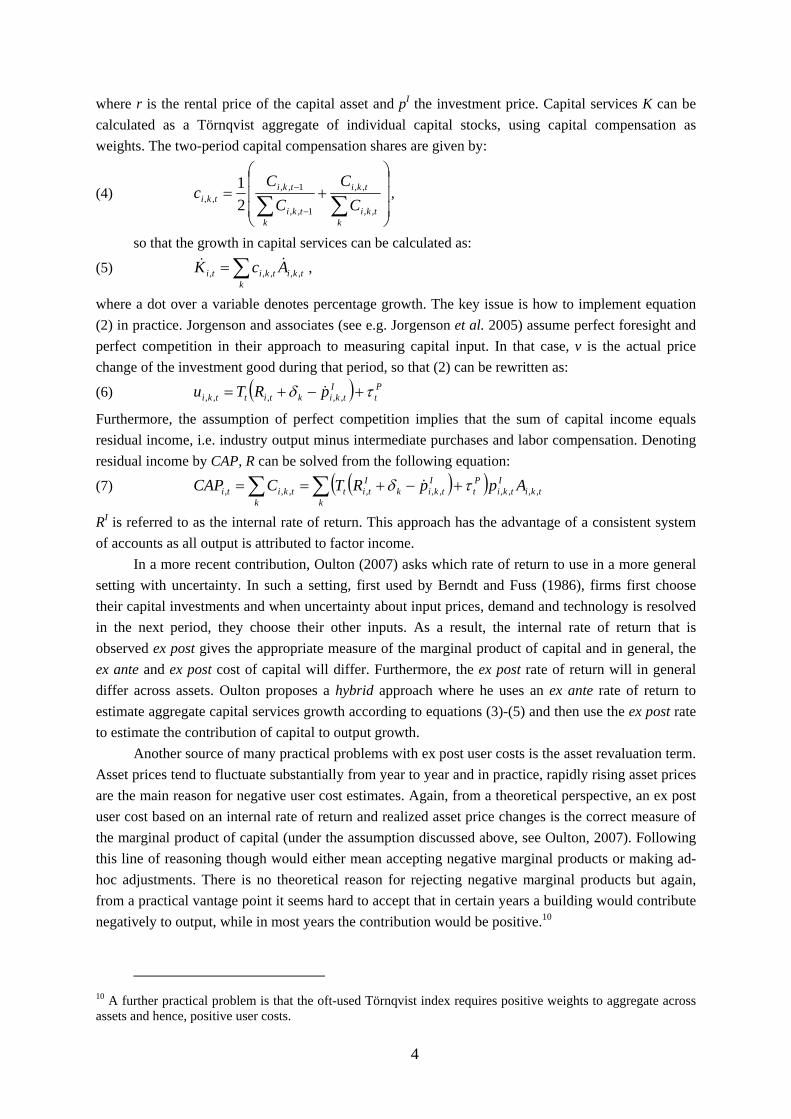
The results show the importance of including intangible assets and the choice for the rate of return. The inclusion of land and inventories and tax parameters are comparatively somewhat less important, but may still merit further study and data collection. The specification chosen for the asset revaluation term and the treatment of negative user costs are of secondary importance. Choosing the rate of return is particularly contentious. On theoretical grounds, one should use an ex-post or internal measure of the rate of return, as was argued by Berndt and Fuss (1986). However, this tends to cause problems in practice, some of which may be related to the assumptions underlying the theoretical framework. The hybrid solution proposed by Oulton (2007) does not solve many of these problems and tends lead to substantially higher growth rates than either the ex-ante or ex-post approach. Using an ex-ante or external measure of the rate of return avoids these issues and is thus preferred from a pragmatic point of view.8 Conceptual framework To frame the discussion, I first discuss the basic approach to capital measurement.9 Given investment (at constant prices) I in industry i, asset k at time t, and geometric depreciation rate �, the capital stock A can be estimated using the perpetual inventory method as follows: (1) ( ) tkitkiktki IAA ,,1,,,, 1 +−= −δ .

We are interested in the service flow from each of the assets rather than the value of assets accumulated and the value of stock A is in general not a good indicator of the contribution of A to overall capital services. For example, buildings make up the largest part of the total stock by value, but the long service life of a building implies a long flow of services from these buildings. To capture the marginal product of a capital asset, a user cost of capital is estimated, following Hall and Jorgenson (1967). This requires assuming that firms are price takers in the market for capital assets and hence, marginal costs equal the marginal product of capital. The basic user cost formula of Hall and Jorgenson (1967) is:

(2) ( ) ( ) Pttkiktitk

Pttkikti

t

tkttktki vRTvR

ZITCu τδτδ

ττ

+−+≡+−+−−−

= ,,,,,,,,,

,, 11

,

with ITC the investment tax credit rate � the corporate tax rate, Z the present value of depreciation allowances, R the rate of return on capital, v the asset revaluation term and �P the property tax rate. How the rate of return and asset revaluation term are implemented in practice will be discussed below. Given the user cost, capital compensation C, or the income stream associated with the asset, can be calculated as:

(3) tkiI

tkitkitkitkitki ApuArC ,,,,,,,,,,,, ≡=

8 Note that this is also the choice made by Statistics Netherlands in their productivity accounts, mostly in order to make the fewest number of theoretical assumptions, see Balk (2008). 9 See other studies for the formal derivations of what follows, e.g. Oulton (2007), Harper, Berndt and Wood (1989) or Berndt and Fuss (1986).

4

where r is the rental price of the capital asset and pI the investment price. Capital services K can be calculated as a Törnqvist aggregate of individual capital stocks, using capital compensation as weights. The two-period capital compensation shares are given by:

(4) ⎟⎟⎟

⎠

⎞

⎜⎜⎜

⎝

⎛+=∑∑ −

−

ktki

tki

ktki

tkitki C

CC

Cc

,,

,,

1,,

1,,,, 2

1,

so that the growth in capital services can be calculated as:

(5) ∑=k

tkitkiti AcK ,,,,,&& ,

where a dot over a variable denotes percentage growth. The key issue is how to implement equation (2) in practice. Jorgenson and associates (see e.g. Jorgenson et al. 2005) assume perfect foresight and perfect competition in their approach to measuring capital input. In that case, v is the actual price change of the investment good during that period, so that (2) can be rewritten as:

(6) ( ) Pt

Itkiktittki pRTu τδ +−+= ,,,,, &

Furthermore, the assumption of perfect competition implies that the sum of capital income equals residual income, i.e. industry output minus intermediate purchases and labor compensation. Denoting residual income by CAP, R can be solved from the following equation:

(7) ( )( )∑∑ +−+==k

tkiI

tkiPt

Itkik

Itit

ktkiti AppRTCCAP ,,,,,,,,,, τδ &

RI is referred to as the internal rate of return. This approach has the advantage of a consistent system of accounts as all output is attributed to factor income.

In a more recent contribution, Oulton (2007) asks which rate of return to use in a more general setting with uncertainty. In such a setting, first used by Berndt and Fuss (1986), firms first choose their capital investments and when uncertainty about input prices, demand and technology is resolved in the next period, they choose their other inputs. As a result, the internal rate of return that is observed ex post gives the appropriate measure of the marginal product of capital and in general, the ex ante and ex post cost of capital will differ. Furthermore, the ex post rate of return will in general differ across assets. Oulton proposes a hybrid approach where he uses an ex ante rate of return to estimate aggregate capital services growth according to equations (3)-(5) and then use the ex post rate to estimate the contribution of capital to output growth.

Another source of many practical problems with ex post user costs is the asset revaluation term. Asset prices tend to fluctuate substantially from year to year and in practice, rapidly rising asset prices are the main reason for negative user cost estimates. Again, from a theoretical perspective, an ex post user cost based on an internal rate of return and realized asset price changes is the correct measure of the marginal product of capital (under the assumption discussed above, see Oulton, 2007). Following this line of reasoning though would either mean accepting negative marginal products or making ad-hoc adjustments. There is no theoretical reason for rejecting negative marginal products but again, from a practical vantage point it seems hard to accept that in certain years a building would contribute negatively to output, while in most years the contribution would be positive.10

10 A further practical problem is that the oft-used Törnqvist index requires positive weights to aggregate across assets and hence, positive user costs.

5

As mentioned above, a theoretically consistent ex post rate of return will in general differ across assets, making an empirical implementation impossible (Oulton, 2007). The next best thing for those who want to stay as close as possible to the theoretical framework would be to use the internal rate of return based on equation (7) in combination with actual annual asset price changes. However, this means that in case of, say, a negative user cost, an alternative interpretation might be that the rate of return on that asset is much higher than the internal rate of return. Trying to avoid the practical problems discussed above by resorting to an ex ante rate and another specification for the asset revaluation term leads to the problem that there are innumerable ad-hoc solutions to choose from. One of the main practical drawbacks of relying on ex post returns is that the contribution of capital to growth is highly influenced by any measurement errors in output (at current prices) and labour compensation. Basu et al. (2008) have shown that at least in finance, current output measurement is by no means without error and estimating the labour compensation of self-employed is also notoriously uncertain.

Regarding the ex ante rate of return, there is some guidance from the literature. Gilchrist and Zakrajsek (2007) use corporate bond data to construct firm-specific user costs of capital and find a strong relationship between this user cost and firm investment. This implies that a rate of return based on financial market data that takes into account the risk associated with investment of firms is a good ex ante cost measure. In the Berndt/Fuss-Oulton models, this cost measure drives investment so on average (i.e. in the absence of shocks), the cost measure should be the same as the ex post return on capital. Harper et al. (1989) use the yield on corporate bonds with a Baa rating as their ex ante measure. Here I use the (risk-free) 10-year Treasury rate plus the risk premium for commercial and industrial loans of US commercial banks based on the Basu, et al. (2008). The main advantage is that this measure is relevant for a larger set of risk profiles of firms. However, the results that follow are very similar if the 10-year Treasury rate had been used without risk adjustment.

There is less guidance when it comes to specifying the asset revaluation term should one want to depart from using current asset price changes. From an ex ante point of view, what matters is the expected asset price change, but this expectation will depend on the (unknown) information set of the firm. Gilchrist and Zakrajsek (2007) use a five-year moving average, but their empirical results do not imply that this is the appropriate specification.11 A wide range of alternatives have been used, such as the average price change across assets or ARMA models (Oulton, 2007).12 Given this situation, it seems most sensible to compare a number of alternatives and evaluate their impact on capital services growth and the occurrence of negative user costs. If these negative user costs do occur, it is desirable from an index number perspective to make ad-hoc adjustments. Again, a number of plausible alternatives can be formulated and their impact can be tested. Data For the empirical analysis that follows, I use data for the United States as this allows for the widest range of scenarios to be examined. The core data consists of investment at current and constant prices in 47 assets for each of 30 industries in the EU KLEMS database for the period 1901-2006. These

11 Their analysis basically explains differences in investment across firms, so the specification of the expected asset price change (which is invariant across firms) cannot be validated from this exercise. 12 Using the average price change across assets is equivalent to using a constant real rate of return as advocated by Diewert (2004), see Harper et al. (1989). Also see Harper et al. (1989) for a more extensive review of the literature on the specification of the asset revaluation term.

6

data are mostly based on the detailed fixed asset tables published by the BEA on 46 non-residential fixed assets. We supplement these data with information on investment by the government and investment in residential buildings.13 We then classify these investment series to the EU KLEMS industries.14 I have chosen to use the set of EU KLEMS industries as this is the most relevant for international comparisons. The analysis itself focuses on the 1977-2005 period as all the complementary data are available for this period.

The data on investment in fixed reproducible assets (henceforth referred to as BEA assets) is supplemented by data on residual income CAP from the EU KLEMS database. In the BEA GDP by Industry Accounts, no distinction is made between net taxes on products and net taxes on production. Therefore, this CAP measure does not conform to the theoretically preferable basic prices concept, which would include net taxes on production but exclude net taxes on products. Our source for the tax parameters (see equation (2)) is the BLS. These data cover the period 1987-2005 and we assume constant tax parameters for the 1977-1987 period. The BLS also provide data on stocks of land and inventories. Here, we were able to combine the data for the 1987-2005 period with data based on the old SIC87 industrial classification for the 1977-1987 period. The BLS in turn uses data on inventories from the BEA and Census as their source. Data on land capital stocks is subject to more assumptions. A study for counties in Ohio from 2001 provides information about the value of land relative to the value of structures by industry and this land-structures ratio is used for the entire period. Land prices are set equal to the average price of structures (see BLS, 1997, 2007). It would obviously be preferable to have more current information about the importance of land in production, but the discussion in Jorgenson, Ho and Stiroh (2005, p. 166) suggests this is problematic. For the final set of capital data, I use newly available estimates of investment in intangible assets from Corrado, Hulten and Sichel (2006). This adds data on investment in computerized information, scientific R&D, non-scientific R&D, brand equity and firm-specific resources. Currently, these data are only available for the private US economy, but for the comparison of aggregate capital services growth, this is already quite useful.

In addition to capital data, income are needed to estimate internal rates of return (CAP from equation (7)). Here I use the data as published in the EU KLEMS database.15 This has the advantage of consistency across countries, partly because the same industry classification is used as in Europe but also because the price concepts are more comparable. CAP is calculated by subtracting labour compensation from value added. Value added as given by the BEA in the GDP by Industry accounts includes net taxes on products and production.16 However, from a production-theory point of view, net taxes on products, such as sales taxes in the US, should be excluded. Net taxes on production, mainly property taxes in the US, should be included however. A breakdown between

13 The BEA data on government investment are only available for a number of types of buildings and overall equipment and software. To distinguish between different types of equipment and software, data on government investment from the 1997 Use table is used in combination with the 1997 Capital Flow Table to bridge investment in commodities to investment in BEA capital assets. This asset distribution is held constant over the sample period, in part because older Use tables did not count software expenditure as a capital investment. 14 Some EU KLEMS industries, such as motor vehicle trade and repair (NACE 50) are not available in this dataset. We split up industries using data on value added, assuming constant asset shares and assuming constant value added shares before 1977. So in this example, we estimate investment for motor vehicle trade and repair by splitting up wholesale trade, retail trade and other services (which includes motor vehicle repairs). 15 See www.euklems.net. 16 Even though the tax variable in the BEA dataset is referred to as ‘Taxes on production and imports, less subsidies’, but see e.g. Guo and Planting (2007).

7

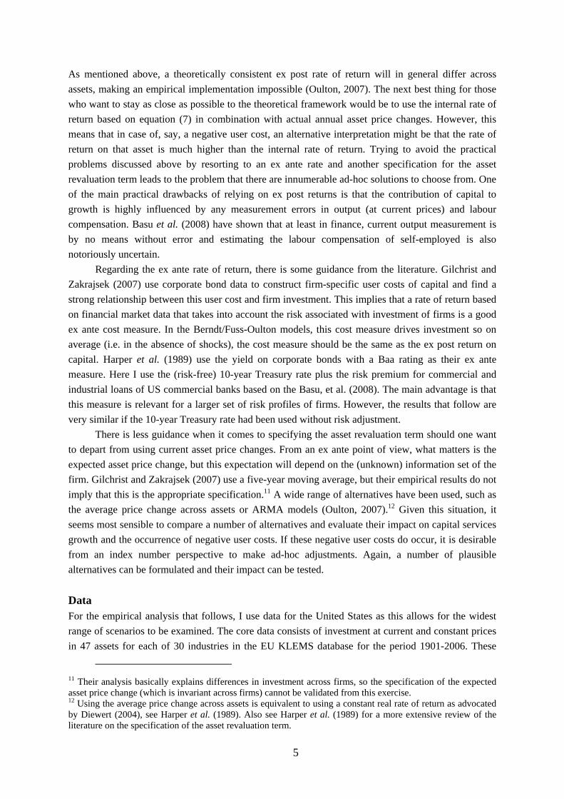
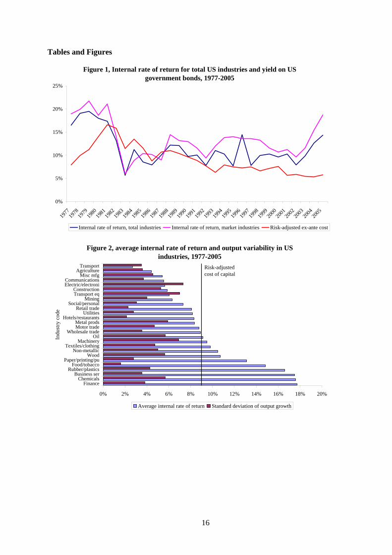
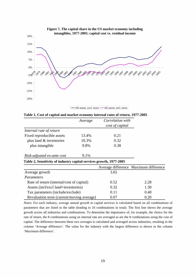
these two types of taxes is only available at the aggregate level. At the industry level, these two types of taxes are distinguished by assuming that all subsidies are subsidies on production and that an industry pays taxes on production in proportion with the industry’s share in the capital stock of structures. Taxes on products are then calculated as a residual.17 Labour compensation of employees is also directly available from the BEA dataset but an imputation needs to be made for the labour compensation of self-employed workers. Here I use the assumption that a self-employed worker earns the same average wage as an employee in each industry. Refinements to this have been made, for example by taking the characteristics (age, sex, education) of self-employed workers into account or by separately estimating capital income and using capital and labour income estimates to divide up non-corporate income.18 Results In analyzing these data, I follow a bottom-up approach. I first analyze the rates of return and asset prices, before turning to the implications of these differences for industry-level capital growth and aggregate capital growth. Finally, I look at the contribution of capital to output growth at the industry and aggregate level and the sensitivity to the assumptions made in capital aggregation. Rates of return Figure 1 plots the aggregate internal rate of return for all industries and all market industries in the US for the 1977-2005 period.19 This internal rate is based on the standard set of fixed, reproducible assets, excluding land, inventories and intangible assets. For reference, an estimate of the risk-adjusted cost of capital is also plotted. As discussed before, this cost of capital consists of a 10-year Treasury bond and the risk premium associated with bank loans to business from Basu et al. (2008).20 The figure shows that both the level and pattern over time of the internal rates of return is differ considerably from the cost of capital. While the average cost of capital is only 9 percent over this period, the internal rate across all industries is 12 percent and for market industries it is 13 percent. The time pattern is also different, with for example rising internal rates after 2000, but a declining cost of capital. The total industries series is not the best basis for comparison as part of capital income used in calculation is based on imputed returns to government activities and residential buildings. For market industries, the correlation between the internal rate and the cost of capital is only 0.21.

However, the internal rate of return in Figure 1 suffers from at least one drawback, namely the set of assets that is covered. Table 1 shows the effect of expanding the asset set, first with land and

17 This procedure has as a risk that in some industries, the estimate of taxes on production are so high that taxes on products would be negative. This problem is more widespread if value added shares are used instead of the industry share in the structures capital stock. To avoid negative taxes and ensure that both types of taxes add up to the correct aggregate, an initial estimate of taxes on production is made, which is equal to the amount based on the share in structures capital or equal to total industry taxes. Next, a RAS procedure is used to ensure industry taxes add up to the correct aggregate. 18 The first method is applied in Jorgenson et al. (2005), the second by the BLS (1997). 19 Market industries excludes government, health and education because much of their output is not directly observed in the market, which means an internal rate estimate is mostly based on the rate that the statistical office imputed for this industry. The real estate industry is also excluded because the imputed rental value of owner-occupied housing makes up most of the output of this industry. 20 The government bond is the constant maturity series from the Federal Reserve interest rate statistics. The risk premium is based on the yield spread of commercial paper of Treasury bills, adjusted to reflect the higher average riskiness of the average bank loan over commercial paper.

8

inventories and then with intangibles. Including land and inventories leads to a substantial decline in the internal rate. This is to be expected as the capital stock increases, while capital income stays the same. The effect of adding intangible investment is smaller because it involves reclassifying expenditure on certain services as investment, so capital income also rises. The overall result of adding these assets is to decrease the gap between the internal rate and the cost of capital to less than a percentage point and the correlation also increases considerably.

This suggests that the aggregate internal rate of return is reasonably comparable to the cost of capital, but only once all assets are measured. The industry detail in this dataset provides a further ground for testing the economic relevance of an internal rate of return. Since intangible investment data is not yet available at the industry level, the internal rates are calculated based on all reproducible fixed assets, land and inventories. It turns out that in almost two-thirds of the 26 market industries, the internal rate of return has a positive correlation with the cost of capital and the average correlation is 0.10.

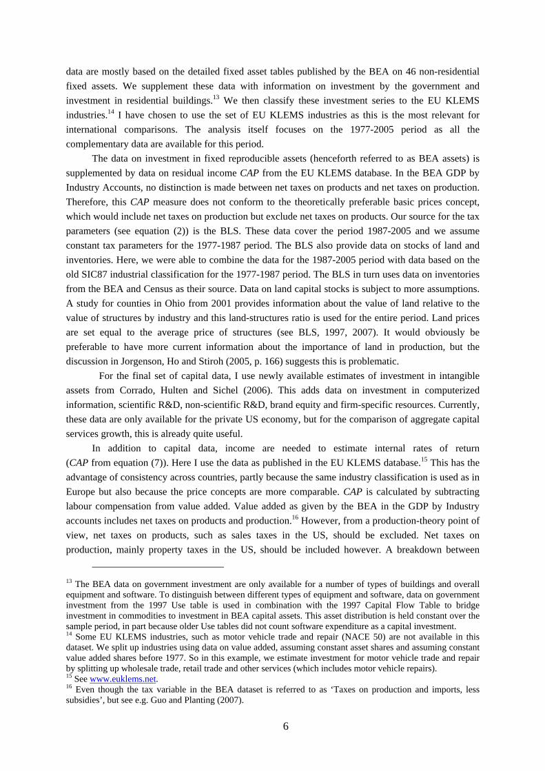
Figure 2 shows the average internal rate for each industry over the entire period. The first observation is that there is considerable heterogeneity between industries. For example, the transport industry shows an average internal rate of only 3 percent and the finance industry a rate of almost 18 percent.21 Also, in most industries, the average internal rate is actually lower than the average cost of capital. This is not just caused by the early 1980s, when most industries had an rate of return lower than the cost of capital, but occurs in many other years as well.

Figure 2 also shows information on the relative risk of an industry, based on the standard deviation of real output growth. The information in the figure already shows little positive relationship, with some industries with highly variable output growth, like transport equipment, showing low returns and firms with stable output (food and tobacco) showing high returns. The correlation between the two series is only -0.13. Alternative explanations for the pattern of internal rate are not immediately convincing either. A lack of competition could also lead to higher internal rates, but a comparison of concentration ratios and internal rates shows no positive correlation either.22 Of course, these are just one indicator of risk and one of competition, but it does raise the question what can explain the large differences in rates of return across industries. Aside from these broader concerns about what the internal rate of return measures and reflects, a more pragmatic concern is that for many countries, data on the stock of land and inventories is not easily available. Even in the US, the data on the stock of land is subject to more assumptions and estimations than other types of capital. However, internal rates based on an incomplete set of assets are too high compared to the cost of capital (Table 1). The relationship over time between the cost of capital and industry-level internal rates also becomes weaker once land and inventories are omitted.23 The broader significance of these concerns for capital measurement will be discussed below.

21 The internal rate of return for finance is overstated however. Much of the output of banks is estimated and as Basu et al. (2008) show, current statistical methods overstate bank output considerably. Their estimates of bank output imply an internal rate of return much closer to that of the market economy. 22 For the concentration ratio the revenue share of the four largest firms in 2002, as given in the Economic Census, is used. 23 In 23 of 26 industries, the correlation is lower.

9

Asset prices Apart from the rate of return R in equation (2), the asset revaluation term v also needs to be implemented. In the Jorgensonian framework discussed above the actual asset price changes are used, but this poses problems similar to the use of an internal rate of return. Under uncertainty, actual asset price changes will have both a random and systematic component. Over long periods of time, investment prices of equipment tend to decline relative to other prices (e.g. Greenwood, Hercowitz and Krussel, 1997), but short-run fluctuations can distort this expected pattern.

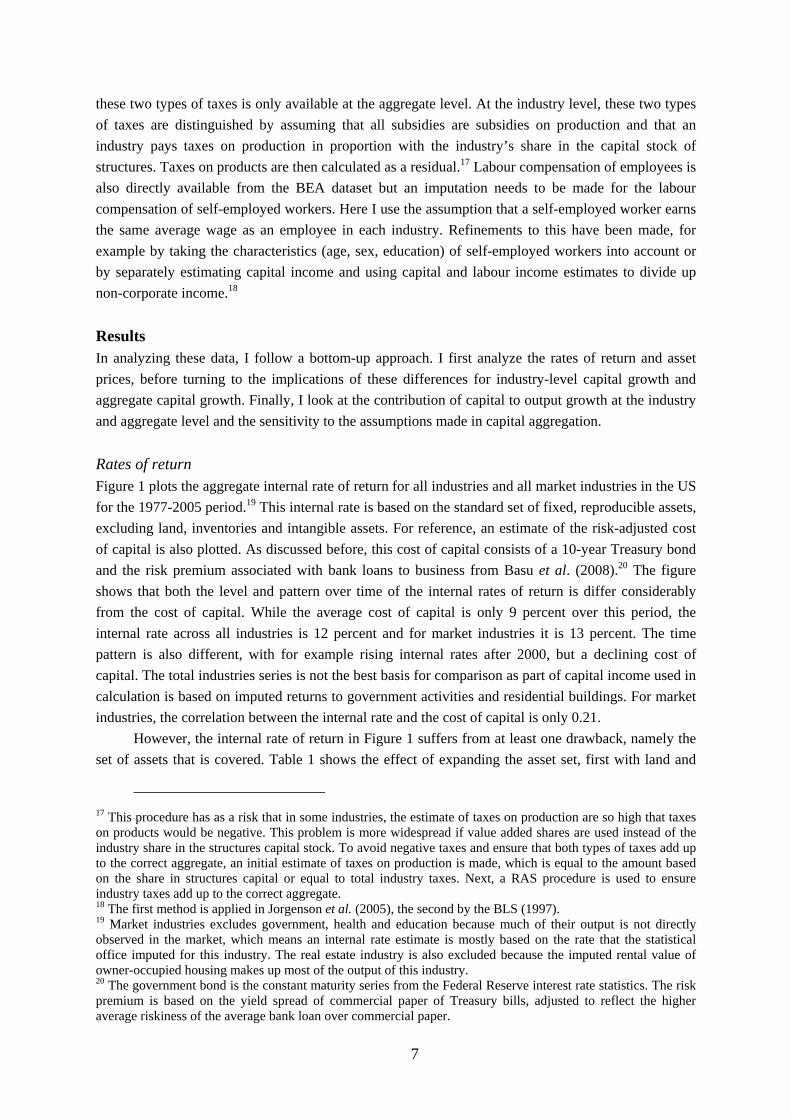
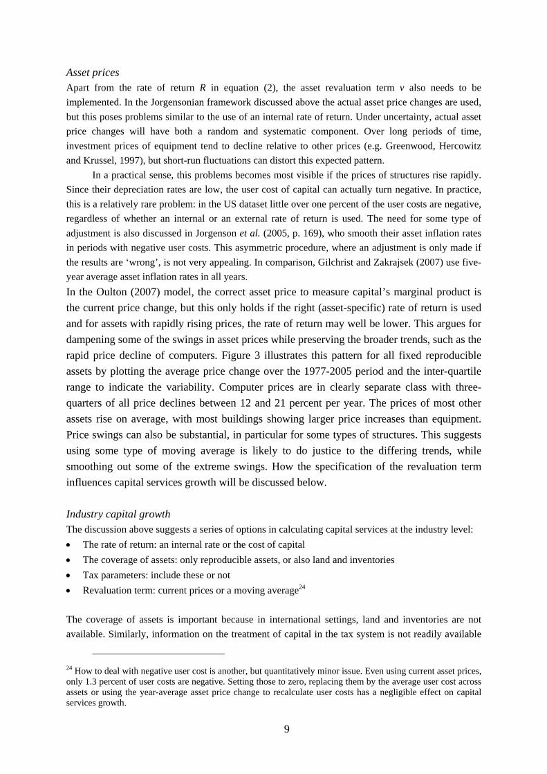
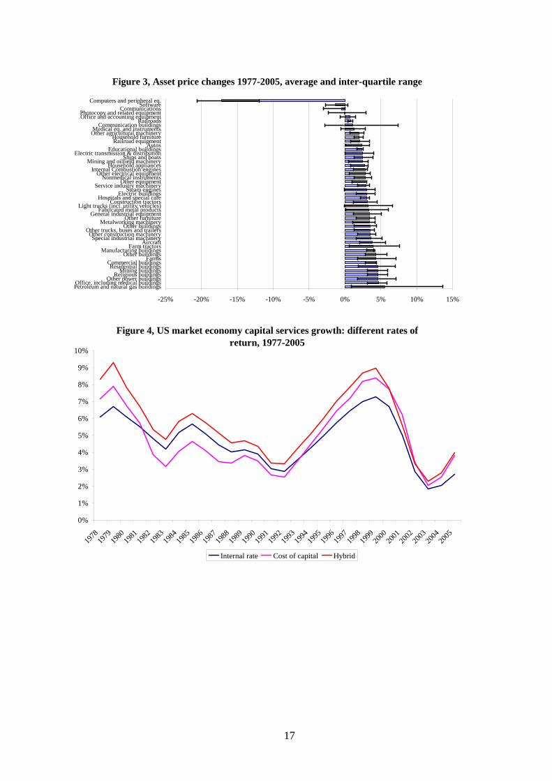
In a practical sense, this problems becomes most visible if the prices of structures rise rapidly. Since their depreciation rates are low, the user cost of capital can actually turn negative. In practice, this is a relatively rare problem: in the US dataset little over one percent of the user costs are negative, regardless of whether an internal or an external rate of return is used. The need for some type of adjustment is also discussed in Jorgenson et al. (2005, p. 169), who smooth their asset inflation rates in periods with negative user costs. This asymmetric procedure, where an adjustment is only made if the results are ‘wrong’, is not very appealing. In comparison, Gilchrist and Zakrajsek (2007) use five-year average asset inflation rates in all years. In the Oulton (2007) model, the correct asset price to measure capital’s marginal product is the current price change, but this only holds if the right (asset-specific) rate of return is used and for assets with rapidly rising prices, the rate of return may well be lower. This argues for dampening some of the swings in asset prices while preserving the broader trends, such as the rapid price decline of computers. Figure 3 illustrates this pattern for all fixed reproducible assets by plotting the average price change over the 1977-2005 period and the inter-quartile range to indicate the variability. Computer prices are in clearly separate class with three-quarters of all price declines between 12 and 21 percent per year. The prices of most other assets rise on average, with most buildings showing larger price increases than equipment. Price swings can also be substantial, in particular for some types of structures. This suggests using some type of moving average is likely to do justice to the differing trends, while smoothing out some of the extreme swings. How the specification of the revaluation term influences capital services growth will be discussed below. Industry capital growth The discussion above suggests a series of options in calculating capital services at the industry level: • The rate of return: an internal rate or the cost of capital • The coverage of assets: only reproducible assets, or also land and inventories • Tax parameters: include these or not • Revaluation term: current prices or a moving average24

The coverage of assets is important because in international settings, land and inventories are not available. Similarly, information on the treatment of capital in the tax system is not readily available

24 How to deal with negative user cost is another, but quantitatively minor issue. Even using current asset prices, only 1.3 percent of user costs are negative. Setting those to zero, replacing them by the average user cost across assets or using the year-average asset price change to recalculate user costs has a negligible effect on capital services growth.

10

for most countries either. The specification of the rate of return and the asset revaluation term are mostly important to see evaluate the importance of the methodological debate on these issues. With four different parameters and two options per parameter, there are 16 different options for 26 different industries and 29 years. To make the analysis manageable, I focus on the average growth in capital services across all years. For increased insight, I will compare the average growth between each of the two options for each parameter, holding the other parameters constant. Of the 16 options, half include tax parameters and half exclude them, so the average growth between these two sets can be compared.

Table 2 shows the results of this comparison. The first row shows an average growth in capital services across all industries and options of 3.65 percent per year. The choice between an internal rate of return and the cost of capital is most important, with average absolute difference in growth between the two of 0.52 percentage points. In most industries, using the cost of capital leads to higher average growth. This is because the cost of capital is lower on average, which means the share in capital compensation of short-lived ICT assets is greater and these assets have shown faster growth over the period. The difference is largest in ICT intensive industries like finance and business services.

Whether land and inventories are included is somewhat less important on average, with an average absolute difference of 0.32 percentage points. The differences are also more concentrated in a few industries. The difference is largest in finance, where including land and inventories subtracts 1.3 percentage points from average growth, followed by agriculture where it adds 1.2 percentage points. In other industries, like hotels and restaurants, the effect is negligible. Taking the tax system into account is already a minor issue, with an average impact of 0.11 percentage points. The effect is largest in finance and in business services, mostly because capital services growth is highest in these industries.

The specification of the revaluation term matters even less for average growth. The difference between using the current asset price change and a five-year moving average is only 0.07 percentage points. It also does not substantially smooth the resulting capital growth series: the average standard deviation of capital growth is 2.62 percent and the difference between current asset prices and a five-year moving is only 0.10 percentage points on average. In contrast, the choice between an internal rate of return and the cost of capital leads to an average absolute difference in the standard deviation of 0.36 percentage points.

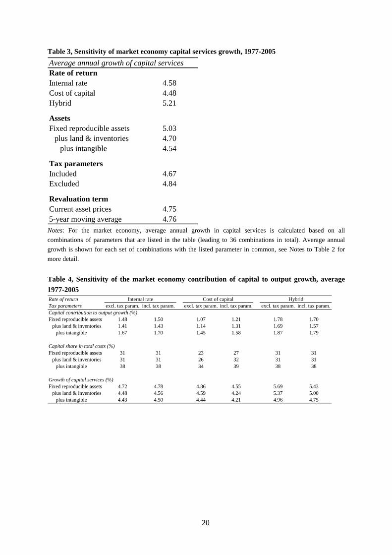
Finally, it is useful to examine the effect of using an internal rate of return with an incomplete set of assets compared to a more complete set. As Table 1 showed, omitting land and inventories leads to an overstatement of the internal rate, so the difference in capital services growth between the internal rate and the cost of capital should be larger if land and inventories are omitted. This is indeed the case, but it is quantitatively less important. The difference in capital growth between an internal rate and the cost of capital is 0.47 percentage points if land and inventories are included and 0.58 if they are omitted. Aggregate capital growth In addition to the aggregation options at the industry level, there is also Oulton’s (2007) proposal to consider for estimating aggregate capital services growth. He proposes a hybrid between using an internal and external rate of return, where the external rate (i.e. the cost of capital) is used to aggregate across assets and internal rates are used to aggregate across industries. Furthermore, at the market economy level, intangible assets can also be included. Table 3 shows the average growth rates for each of the parameters, averaging over the results based on the other parameters as in Table 2. This

11

table shows how the main findings from the industry-level also show up at the aggregate. The specification of the revaluation term matters very little: average growth is 4.75 percent either way. Including tax parameters decreases capital growth by 0.19 percentage points, a bigger effect than for most industries, but modest given overall growth. Again, the set of assets and the rate of return matter most. The widest asset boundary, including both land and inventories and intangibles, shows the slowest average growth of only 4.53 percent. This is half a percentage point lower than if those assets were excluded. The growth based on the internal rate and the cost of capital seem surprisingly close compared to the differences shown in Table 2. Moreover, growth based on an internal rate is actually higher than based on the cost of capital, even though the reverse tended to be the case at the industry level. The reason for this is that industries like finance and business services might have lower growth rates using an internal rate of return, but their growth is still considerably higher than the average. Furthermore, their high internal rates of return (cf. Figure 2) imply that the share of the industry in total residual income CAP is much higher than that based on the cost of capital. These two effects partly cancel out, but the increase in the industry capital share outweighs the decrease in industry growth. This also explains why the hybrid option leads to higher aggregate growth than both alternatives: it combines high industry growth with a higher share of high-growth industries.

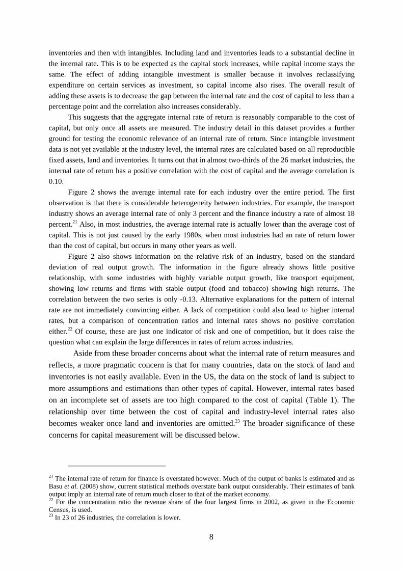
In addition to the period averages, it can be useful to compare the growth pattern over time for a number of alternatives. As the specification of the revaluation term matters very little, I use current asset prices since this is the most straightforward in practice. Similarly, I omit tax parameters. Figure 4 compares aggregate growth calculated using different rates of return based on the set of fixed reproducible assets. First of all, the hybrid option shows higher growth in almost every year than the other two option. Furthermore, even though the average growth based on internal rates and the cost of capital is very similar, differences are larger in some periods than others. In particular, during the ICT investment boom in the late-1990s, aggregate growth was around a percentage point higher based on the cost of capital than on internal rates, while it was a percentage point lower in the late-1980s. The comparison is similar for the set of assets including land and inventories.

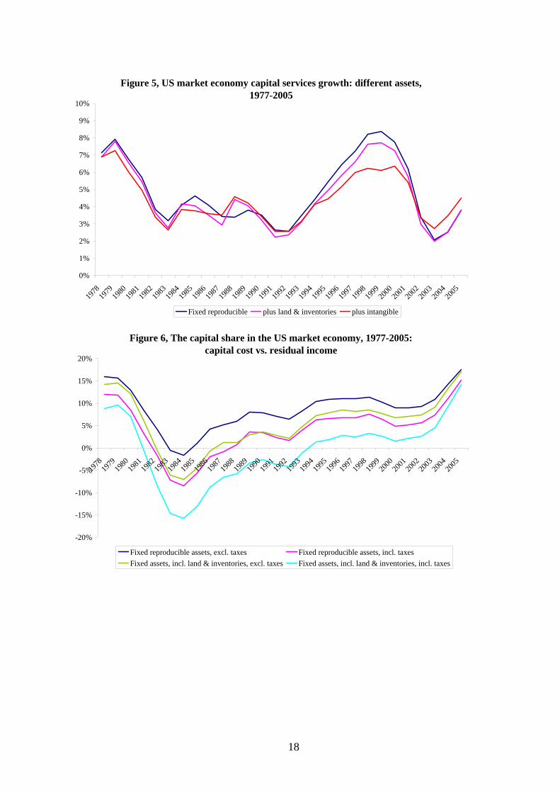
Figure 5 compares growth based on the three different set of assets from Table 3 and shows that the main differences are in the late-1990s.25 If land and inventories are included, growth is about half a percentage point lower while also including intangible assets, lowers growth by about two percentage points in total. After 2000 though, growth with intangibles are included is 0.5-1 percentage points higher. In summary, the choice for the rate of return and the set of assets that is covered matters substantially at the industry level and the aggregate level. Moreover, the differences are not constant over time. The contribution of capital to growth The analysis from the previous sections has established the quantitative importance for capital services growth of different approaches to capital aggregation across assets and industries. As these data are often used in growth accounting, it is useful to place the results in a broader context. In growth accounting, the contribution of capital is estimated as the share of capital in total costs time the growth of capital. Under perfect competition, total costs equal total output, but as long as returns to scale are constant, the more general expression holds (Hall, 1990).

25 Figure 5 is based on the external rate of return. The comparison is very similar for the other options for the rate of return.

12

The first issue is how the contribution of capital to growth varies depending on the set of assets that is covered. The combination of an internal rate of return and an incomplete set of assets is likely to be particularly problematic as the underlying assumption is that all residual income CAP can be attributed to the income from the set of assets that is covered. The second issue is how capital compensation estimated using the cost of capital compares to value added. Since in this approach capital compensation does not add up to residual income CAP, there will be economic profits or losses and it should be informative to evaluate its size and pattern over time.

Table 4 shows the results for the contribution of capital to market economy growth of value added. The top panel of the table shows the contribution of capital to output growth, the middle panel shows the share of capital in total costs and the bottom panel shows the growth of capital services.26 Current asset prices are used for the revaluation term throughout. The first column shows that when using internal rates of return and excluding tax parameters, growth of capital has contributed 1.48 percentage points to output growth if only fixed reproducible assets are covered. This contribution drops to 1.41 if land and inventories are included and rises to 1.67 if intangibles are included as well. The contributions are almost identical if tax parameters are included. The pattern is also similar for the hybrid case, except that the contributions are higher because of a higher growth in capital services. In both cases, including land and inventories decreases the contribution because growth of those assets is slower than average while the amount of capital income is unchanged at 31 percent of value added (since total costs equal output in both cases). Including intangibles adds around 11 percent to GDP, leading to a capital share that is 7 percentage points higher, so even though capital growth including intangibles is lower (cf. Table 3), the contribution of capital to output growth is higher.

Using the cost of capital in calculating user costs leads to a monotonically increasing contribution of capital if more assets are covered, since capital compensation increases with each addition. However, the contribution to output growth is always lower than in the other two rate of return options. The reasons for this vary, but for the case when only fixed reproducible assets included, the lower capital share is the main reason compared to the internal rate of return. Adding more assets and including tax parameters decrease the gap until the point where, in terms of the average contribution, using internal rates or the cost of capital matters little. Unlike for the other options, including tax parameters is an important factor, mostly because it increases the capital share. The results also illustrate the bias in estimating the capital contribution by using an incomplete set of assets in combination with internal rates of return. While the cost of capital contributions show that fixed reproducible assets contribute at most 1.21 percentage points to output growth, the internal rate estimates imply a contribution of about 1.5 percentage points.

The differences in contribution are also vary stable over time with the contribution based on the cost capital the lowest and the hybrid the highest with the internal rate as an intermediate version. Figure 6 shows a more revealing picture, comparing the capital share based on residual income CAP to the capital shares implied by using the cost of capital to estimate capital compensation, all without taking intangible assets into account. The residual income share is fairly constant over this period, varying between 30 and 34 percent of output, while capital compensation is much more variable. The figure shows the difference between these two concepts for four cases, namely including and

26 Note that for the internal rate and hybrid options, the average annual growth in capital services time the average capital share is almost equal to the average annual contribution. The difference is more noticeable for the cost of capital because, as discussed below, the capital share is more variable.

13

excluding land and inventories and including and excluding tax parameters. The basic pattern is similar in these four series but the differences in the level is considerable. In most years, the difference is positive, implying that residual income is larger than capital compensation, but in the mid-1980s, capital costs were so high that capital compensation was larger than residual income. The most comprehensive capital compensation measure, including land and inventories and tax parameters is higher than residual income for 13 of the years covered, implying substantial economic losses. Figure 7 shows that also including intangibles leads to a very similar picture, except that underlying residual income increases from around 35 to 41 percent of output.

At the industry level, the difference between residual income and capital compensation closely mirrors the pattern of internal rates of return from Figure 2. This is of course no surprise since an internal rate in excess of the cost of capital signifies that residual income is higher than the compensation required for the capital stock. The number of industries with higher capital compensation than residual income on average over the entire period varies substantially between the different alternatives. If tax parameters and land and inventories are excluded, only the transport and storage industry has higher capital compensation than residual income but if both are included capital compensation is higher in 14 of 26 industries.

As was the case for the internal rate of return, there do not seem to be straightforward explanations what can explain the wide disparity, both over time and across industries. In all likelihood, measures of risk and competition factor into the equation. Measurement errors also cannot be ignored. Since CAP is calculated as residual income, any measurement problems in output or labour compensation end up here. The estimation of self-employed labour compensation is a particularly important source of uncertainty here. Data on investment and capital income are also not collected from the same sources and since capital services are not (yet) part of the National Accounts, any discrepancies between sources is not taken into account in the reconciliation process by statistical offices. These measurement issues suggest that caution is needed, in particular in interpreting industry-level results but also at the aggregate level.

Despite these health warnings, a number of observations stand out from the analysis of capital contributions to output growth. First, the combination of internal rates of return and an incomplete set of assets can lead to misleading results as it implies too large a contribution of fixed reproducible assets. Using the cost of capital is less hazardous in this respect, but necessitates a careful consideration of the tax system to avoid underestimating the share of capital in total costs. Finally, the hybrid solution proposed by Oulton (2007) implies much higher capital contributions to output growth than any of the other methods. Conclusions Measuring capital is hard. Economic theory is a useful guide for part of the way but as illustrated by Oulton (2007), sooner or later choices have to be made on pragmatic grounds. The aim of this paper has been to illuminate the impact of these choices to focus attention and hopefully research on the most pressing issues. Some issues have not been dealt with here: time series for investment by industry and assets in both current and constant prices have been taken as given. I have also not discussed depreciation rates and to what extent we should rely on them. For these and other issues related to capital measurement, see the OECD Manual (Schreyer, 2008). This paper has taken industry capital stocks by asset as given and asked how these should be aggregated to get an informative measure of productive capital input into production.

14

Central in this aggregation problem is the user cost of capital, which consists of a rate of return, depreciation rate, revaluation term and tax parameters. For each of these components different choices and assumptions can be justified and I compare how these choices impact the results. It turns out that many of the choices matter only little. For example, instead of using the current asset price change for the revaluation term, moving averages can be specified but this matters little. What is important is that asset-specific price changes should be taken into account as in particular, computer prices have fallen very rapidly and this is part of the user cost of capital.

The choice for the rate of return is more consequential. Estimates of the internal rate of return are not easy to reconcile with economic fundamentals such as the relative risk of industries or the cost of capital in financial markets. This suggests broader measurement problems are important: the internal rate of return will only be an economically useful concept if capital income is measured in a fully correct fashion and all relevant capital assets are correctly accounted for. Neither of these is likely in practice. Oulton’s (2007) hybrid approach does not solve this issue and hence, I would favour Balk’s (2008) argument for an external rate of return.

This means capital cost does not fully exhaust revenue and the size of capital costs will vary depending on whether tax parameters are included and which assets are covered. At the aggregate level, on average over time, capital cost is comparable in size to residual income once taxes are accounted for and land and inventories are covered. Not accounting for either of these will understate the contribution of capital input growth to output growth. Finally, most intangible assets are not yet considered part of the standard set of capital assets and there are many conceptual issues. For example, the question how and how much knowledge (in the form of R&D) depreciates is still not answered in a satisfactory fashion. However, using the same assumptions as Corrado et al. (2006) shows that including intangible assets is very important as well.

15

References

Balk, B.M. (2008), “Measuring Productivity Change without Neoclassical Assumptions: A Conceptual Analysis” mimeo.

Basu, S., R. Inklaar and J.C. Wang (2008), “The Value of Risk: Measuring the Service Output of U.S. Commercial Banks” mimeo.

Berndt, Ernst R. and Melvin A. Fuss (1986), “Productivity Measurement with Adjustments for Variations in Capacity Utilizations and Other Forms of Temporary Equilibrium” Journal of Econometrics, 33(1), pp. 7-29.

BLS (1997), BLS Handbook of Methods, BLS Bulletin 2490, US Department of Labor: Washington D.C.

BLS (2007) Technical Information About the BLS Multifactor Productivity Measures, US Department of Labor: Washington D.C.

Corrado, C.A., C.R. Hulten and D.E. Sichel (2006), “Intangible Capital and Economic Growth” NBER Working Paper, no. 11948.

Diewert, W.E. (2004), “Issues in the Measurement of Capital Services, Depreciation, Asset Price Changes and Interest Rates” UBC Discussion Paper 04-11.

Diewert, W.E (2008), “What is to be done for better productivity measurement” International Productivity Monitor 16, pp. 40-52.

Erumban, A.A. (2008), “Rental Prices, Rates of Return, Capital Aggregation and Productivity: Evidence from EU and US” forthcoming in CESifo Economic Studies.

Gilchrist, S. and E. Zakrajsek (2007), “Investment and the cost of capital: New evidence from the corporate bond market” NBER Working Paper, no. 13174.

Greenwood, J., Z. Hercowitz and P. Krussel (1997), “Long-Run Implication of Investment-Specific Technological Change” American Economic Review, 87(3) pp. 342-362.

Guo, J. and M.A. Planting (2007), “Integrating U.S. Input-Output Tables with SNA: Valuations and Extensions” paper presented at the 16th International Input-Output Conference in Istanbul, Turkey, July 2-7 2007.

Hall, R.E. and D.W. Jorgenson (1967), “Tax Policy and Investment Behavior” American Economic Review, 57(3) pp. 391-414.

Hall, Robert E. (1990), “Invariance Properties of Solow’s Productivity Residual” In Peter A. Diamond (ed.) Growth/Productivity/Employment: Essays to Celebrate Bob Solow’s Birthday, MIT Press: Cambridge.

Harper, M.J., E.R. Berndt and D.O. Wood (1989), “Rates of Return and Capital Aggregation Using Alternative Rental Prices” in Jorgenson and Landau (eds.) Technology and Capital Formation, pp. 331-372, MIT Press: Cambridge.

Jorgenson, D.W. and Z. Griliches (1967), “The Explanation of Productivity Change” Review of Economic Studies, 34(3) pp. 249-283.

Jorgenson, D.W., M.S. Ho, and K.J. Stiroh (2005), Information Technology and the American Growth Resurgence, Cambridge, The MIT Press.

Oulton, N. (2007), “Ex post versus ex ante measures of the user cost of capital” Review of Income and Wealth, 53(2) pp. 295-317.

Schreyer, P. (2008), OECD Manual Measuring Capital, draft version, OECD: Paris

16

Tables and Figures

Figure 1, Internal rate of return for total US industries and yield on US government bonds, 1977-2005

0%

5%

10%

15%

20%

25%

1977

1978

1979

1980

1981

1982

1983

1984

1985

1986

1987

1988

1989

1990

1991

1992

1993

1994

1995

1996

1997

1998

1999

2000

2001

2002

2003

2004

2005

Internal rate of return, total industries Internal rate of return, market industries Risk-adjusted ex-ante cost

Figure 2, average internal rate of return and output variability in US industries, 1977-2005

0% 2% 4% 6% 8% 10% 12% 14% 16% 18% 20%

FinanceChemicals

Business serRubber/plastics

Food/tobaccoPaper/printing/pu

WoodNon-metallic

Textiles/clothingMachinery

OilWholesale trade

Motor tradeMetal prods

Hotels/restaurantsUtilities

Retail tradeSocial/personal

MiningTransport eqConstruction

Electric/electroniCommunications

Misc mfgAgriculture

Transport

Indu

stry

cod

e

Average internal rate of return Standard deviation of output growth

Risk-adjusted cost of capital

17

Figure 3, Asset price changes 1977-2005, average and inter-quartile range

-25% -20% -15% -10% -5% 0% 5% 10% 15%

Petroleum and natural gas buildingsOffice, including medical buildingsOther power buildings

Religious buildingsMining buildings

Residential buildingsCommercial buildings

FarmsOther buildings

Manufacturing buildingsFarm tractors

AircraftSpecial industrial machineryOther construction machinery

Other trucks, buses and trailersOther buildings

Metalworking machineryOther furniture

General industrial equipmentFabricated metal products

Light trucks (incl. utility vehicles)Construction tractors

Hospitals and special careElectric buildingsSteam engines

Service industry machineryOther equipment

Nonmedical instrumentsOther electrical equipment

Internal Combustion enginesHousehold appliances

Mining and oilfield machineryShips and boats

Electric transmission & distributionEducational buildingsAutos

Railroad equipmentHousehold furniture

Other agricultural machineryMedical eq. and instruments

Communication buildingsRailroads

Office and accounting equipmentPhotocopy and related equipment

CommunicationsSoftwareComputers and peripheral eq.

Figure 4, US market economy capital services growth: different rates of return, 1977-2005

0%

1%

2%

3%

4%

5%

6%

7%

8%

9%

10%

1978

1979

1980

1981

1982

1983

1984

1985

1986

1987

1988

1989

1990

1991

1992

1993

1994

1995

1996

1997

1998

1999

2000

2001

2002

2003

2004

2005

Internal rate Cost of capital Hybrid

18

Figure 5, US market economy capital services growth: different assets, 1977-2005

0%

1%

2%

3%

4%

5%

6%

7%

8%

9%

10%

1978

1979

1980

1981

1982

1983

1984

1985

1986

1987

1988

1989

1990

1991

1992

1993

1994

1995

1996

1997

1998

1999

2000

2001

2002

2003

2004

2005

Fixed reproducible plus land & inventories plus intangible

Figure 6, The capital share in the US market economy, 1977-2005: capital cost vs. residual income

-20%

-15%

-10%

-5%

0%

5%

10%

15%

20%

1978

1979

1980

1981

1982

1983

1984

1985

1986

1987

1988

1989

1990

1991

1992

1993

1994

1995

1996

1997

1998

1999

2000

2001

2002

2003

2004

2005

Fixed reproducible assets, excl. taxes Fixed reproducible assets, incl. taxesFixed assets, incl. land & inventories, excl. taxes Fixed assets, incl. land & inventories, incl. taxes

19

Figure 7, The capital share in the US market economy including intangibles, 1977-2005: capital cost vs. residual income

-20%

-15%

-10%

-5%

0%

5%

10%

15%

20%

1978

1979

1980

1981

1982

1983

1984

1985

1986

1987

1988

1989

1990

1991

1992

1993

1994

1995

1996

1997

1998

1999

2000

2001

2002

2003

2004

2005

All assets, excl. taxes All assets, incl. taxes

Table 1, Cost of capital and market economy internal rates of return, 1977-2005 Average Correlation with

cost of capitalInternal rate of returnFixed reproducible assets 13.4% 0.21

plus land & inventories 10.3% 0.32plus intangible 9.8% 0.38

Risk-adjusted ex-ante cost 9.1% Table 2, Sensitivity of industry capital services growth, 1977-2005

Average difference Maximum differenceAverage growth 3.65Parameters

Rate of return (internal/cost of capital) 0.52 2.28Assets (incl/excl land+inventories) 0.32 1.30Tax parameters (include/exclude) 0.11 0.40Revaluation term (current/moving average) 0.07 0.20

Notes: For each industry, average annual growth in capital services is calculated based on all combinations of parameters that are listed in the table (leading to 16 combinations in total). The first line shows the average growth across all industries and combinations. To determine the importance of, for example, the choice for the rate of return, the 8 combinations using an internal rate are averaged as are the 8 combinations using the cost of capital. The difference between these two averages is calculated and averaged across industries, resulting in the column ‘Average difference’. The value for the industry with the largest difference is shown in the column ‘Maximum difference’.

20

Table 3, Sensitivity of market economy capital services growth, 1977-2005 Average annual growth of capital servicesRate of returnInternal rate 4.58Cost of capital 4.48Hybrid 5.21

AssetsFixed reproducible assets 5.03

plus land & inventories 4.70plus intangible 4.54

Tax parametersIncluded 4.67Excluded 4.84

Revaluation termCurrent asset prices 4.755-year moving average 4.76

Notes: For the market economy, average annual growth in capital services is calculated based on all combinations of parameters that are listed in the table (leading to 36 combinations in total). Average annual growth is shown for each set of combinations with the listed parameter in common, see Notes to Table 2 for more detail. Table 4, Sensitivity of the market economy contribution of capital to output growth, average 1977-2005 Rate of returnTax parameters excl. tax param. incl. tax param. excl. tax param. incl. tax param. excl. tax param. incl. tax param.Capital contribution to output growth (%)Fixed reproducible assets 1.48 1.50 1.07 1.21 1.78 1.70

plus land & inventories 1.41 1.43 1.14 1.31 1.69 1.57plus intangible 1.67 1.70 1.45 1.58 1.87 1.79

Capital share in total costs (%)Fixed reproducible assets 31 31 23 27 31 31

plus land & inventories 31 31 26 32 31 31plus intangible 38 38 34 39 38 38

Growth of capital services (%)Fixed reproducible assets 4.72 4.78 4.86 4.55 5.69 5.43

plus land & inventories 4.48 4.56 4.59 4.24 5.37 5.00plus intangible 4.43 4.50 4.44 4.21 4.96 4.75

Cost of capitalInternal rate Hybrid

21

Papers issued in the series of the Groningen Growth and Development Centre

All papers are available in pdf-format on the internet: http://www.ggdc.net/

536 (GD-1) Maddison, Angus and Harry van Ooststroom, The International Comparison of Value Added, Productivity and Purchasing Power Parities in Agriculture (1993)

537 (GD-2) Mulder, Nanno and Angus Maddison, The International Comparison of Performance in Distribution: Value Added, Labour Productivity and PPPs in Mexican and US Wholesale and Retail Trade 1975/7 (1993)

538 (GD-3) Szirmai, Adam, Comparative Performance in Indonesian Manufacturing, 1975-90 (1993)

549 (GD-4) de Jong, Herman J., Prices, Real Value Added and Productivity in Dutch Manufacturing, 1921-1960 (1993)

550 (GD-5) Beintema, Nienke and Bart van Ark, Comparative Productivity in East and West German Manufacturing before Reunification (1993)

567 (GD-6) Maddison, Angus and Bart van Ark, The International Comparison of Real Product and Productivity (1994)

568 (GD-7) de Jong, Gjalt, An International Comparison of Real Output and Labour Productivity in Manufacturing in Ecuador and the United States, 1980 (1994)

569 (GD-8) van Ark, Bart and Angus Maddison, An International Comparison of Real Output, Purchasing Power and Labour Productivity in Manufacturing Industries: Brazil, Mexico and the USA in 1975 (1994) (second edition)

570 (GD-9) Maddison, Angus, Standardised Estimates of Fixed Capital Stock: A Six Country Comparison (1994)

571 (GD-10) van Ark, Bart and Remco D.J. Kouwenhoven, Productivity in French Manufacturing: An International Comparative Perspective (1994)

572 (GD-11) Gersbach, Hans and Bart van Ark, Micro Foundations for International Productivity Comparisons (1994)

573 (GD-12) Albers, Ronald, Adrian Clemens and Peter Groote, Can Growth Theory Contribute to Our Understanding of Nineteenth Century Economic Dynamics (1994)

574 (GD-13) de Jong, Herman J. and Ronald Albers, Industrial Output and Labour Productivity in the Netherlands, 1913-1929: Some Neglected Issues (1994)

575 (GD-14) Mulder, Nanno, New Perspectives on Service Output and Productivity: A Comparison of French and US Productivity in Transport, Communications Wholesale and Retail Trade (1994)

576 (GD-15) Maddison, Angus, Economic Growth and Standards of Living in the Twentieth Century (1994)

577 (GD-16) Gales, Ben, In Foreign Parts: Free-Standing Companies in the Netherlands around the First World War (1994)

578 (GD-17) Mulder, Nanno, Output and Productivity in Brazilian Distribution: A Comparative View (1994)

579 (GD-18) Mulder, Nanno, Transport and Communication in Mexico and the United States: Value Added, Purchasing Power Parities and Productivity (1994)

22

580 (GD-19) Mulder, Nanno, Transport and Communications Output and Productivity in Brazil and the USA, 1950-1990 (1995)

581 (GD-20) Szirmai, Adam and Ren Ruoen, China's Manufacturing Performance in Comparative Perspective, 1980-1992 (1995)

GD-21 Fremdling, Rainer, Anglo-German Rivalry on Coal Markets in France, the Netherlands and Germany, 1850-1913 (December 1995)

GD-22 Tassenaar, Vincent, Regional Differences in Standard of Living in the Netherlands, 1800-1875, A Study Based on Anthropometric Data (December 1995)

GD-23 van Ark, Bart, Sectoral Growth Accounting and Structural Change in Postwar Europe (December 1995)

GD-24 Groote, Peter, Jan Jacobs and Jan Egbert Sturm, Output Responses to Infrastructure in the Netherlands, 1850-1913 (December 1995)

GD-25 Groote, Peter, Ronald Albers and Herman de Jong, A Standardised Time Series of the Stock of Fixed Capital in the Netherlands, 1900-1995 (May 1996)

GD-26 van Ark, Bart and Herman de Jong, Accounting for Economic Growth in the Netherlands since 1913 (May 1996)

GD-27 Maddison, Angus and D.S. Prasada Rao, A Generalized Approach to International Comparisons of Agricultural Output and Productivity (May 1996)

GD-28 van Ark, Bart, Issues in Measurement and International Comparison of Productivity - An Overview (May 1996)

GD-29 Kouwenhoven, Remco, A Comparison of Soviet and US Industrial Performance, 1928-90 (May 1996)

GD-30 Fremdling, Rainer, Industrial Revolution and Scientific and Technological Progress (December 1996)

GD-31 Timmer, Marcel, On the Reliability of Unit Value Ratios in International Comparisons (December 1996)

GD-32 de Jong, Gjalt, Canada's Post-War Manufacturing Performance: A Comparison with the United States (December 1996)

GD-33 Lindlar, Ludger, “1968” and the German Economy (January 1997) GD-34 Albers, Ronald, Human Capital and Economic Growth: Operationalising Growth

Theory, with Special Reference to The Netherlands in the 19th Century (June 1997) GD-35 Brinkman, Henk-Jan, J.W. Drukker and Brigitte Slot, GDP per Capita and the

Biological Standard of Living in Contemporary Developing Countries (June 1997) GD-36 de Jong, Herman, and Antoon Soete, Comparative Productivity and Structural Change

in Belgian and Dutch Manufacturing, 1937-1987 (June 1997) GD-37 Timmer, M.P., and A. Szirmai, Growth and Divergence in Manufacturing Performance

in South and East Asia (June 1997) GD-38 van Ark, B., and J. de Haan, The Delta-Model Revisited: Recent Trends in the

Structural Performance of the Dutch Economy (December 1997) GD-39 van der Eng, P., Economics Benefits from Colonial Assets: The Case of the

Netherlands and Indonesia, 1870-1958 (June 1998) GD-40 Timmer, Marcel P., Catch Up Patterns in Newly Industrializing Countries. An

International Comparison of Manufacturing Productivity in Taiwan, 1961-1993 (July 1998)

23

GD-41 van Ark, Bart, Economic Growth and Labour Productivity in Europe: Half a Century of East-West Comparisons (October 1999)

GD-42 Smits, Jan Pieter, Herman de Jong and Bart van Ark, Three Phases of Dutch Economic Growth and Technological Change, 1815-1997 (October 1999)

GD-43 Fremdling, Rainer, Historical Precedents of Global Markets (October 1999) GD-44 van Ark, Bart, Lourens Broersma and Gjalt de Jong, Innovation in Services. Overview

of Data Sources and Analytical Structures (October 1999) GD-45 Broersma, Lourens and Robert McGuckin, The Impact of Computers on Productivity in

the Trade Sector: Explorations with Dutch Microdata (October 1999, Revised version June 2000)

GD-46 Sleifer, Jaap, Separated Unity: The East and West German Industrial Sector in 1936 (November 1999)

GD-47 Rao, D.S. Prasada and Marcel Timmer, Multilateralisation of Manufacturing Sector Comparisons: Issues, Methods and Empirical Results (July 2000)

GD-48 Vikström, Peter, Long term Patterns in Swedish Growth and Structural Change, 1870-1990 (July 2001)

GD-49 Wu, Harry X., Comparative labour productivity performance in Chinese manufacturing, 1952-1997: An ICOP PPP Approach (July 2001)

GD-50 Monnikhof, Erik and Bart van Ark, New Estimates of Labour Productivity in the Manufacturing Sectors of Czech Republic, Hungary and Poland, 1996 (January 2002)

GD-51 van Ark, Bart, Robert Inklaar and Marcel Timmer, The Canada-US Manufacturing Gap Revisited: New ICOP Results (January 2002)

GD-52 Mulder, Nanno, Sylvie Montout and Luis Peres Lopes, Brazil and Mexico's Manufacturing Performance in International Perspective, 1970-98 (January 2002)

GD-53 Szirmai, Adam, Francis Yamfwa and Chibwe Lwamba, Zambian Manufacturing Performance in Comparative Perspective (January 2002)

GD-54 Fremdling, Rainer, European Railways 1825-2001, an Overview (August 2002) GD-55 Fremdling, Rainer, Foreign Trade-Transfer-Adaptation: The British Iron Making

Technology on the Continent (Belgium and France) (August 2002) GD-56 van Ark, Bart, Johanna Melka, Nanno Mulder, Marcel Timmer and Gerard Ypma, ICT

Investments and Growth Accounts for the European Union 1980-2000 (September 2002)

GD-57 Sleifer, Jaap, A Benchmark Comparison of East and West German Industrial Labour Productivity in 1954 (October 2002)

GD-58 van Dijk, Michiel, South African Manufacturing Performance in International Perspective, 1970-1999 (November 2002)

GD-59 Szirmai, A., M. Prins and W. Schulte, Tanzanian Manufacturing Performance in Comparative Perspective (November 2002)

GD-60 van Ark, Bart, Robert Inklaar and Robert McGuckin, “Changing Gear” Productivity, ICT and Services: Europe and the United States (December 2002)

GD-61 Los, Bart and Timmer, Marcel, The ‘Appropriate Technology’ Explanation of Productivity Growth Differentials: An Empirical Approach (April 2003)

GD-62 Hill, Robert J., Constructing Price Indexes Across Space and Time: The Case of the European Union (May 2003)

24

GD-63 Stuivenwold, Edwin and Marcel P. Timmer, Manufacturing Performance in Indonesia, South Korea and Taiwan before and after the Crisis; An International Perspective, 1980-2000 (July 2003)

GD-64 Inklaar, Robert, Harry Wu and Bart van Ark, “Losing Ground”, Japanese Labour Productivity and Unit Labour Cost in Manufacturing in Comparison to the U.S. (July 2003)

GD-65 van Mulligen, Peter-Hein, Alternative Price Indices for Computers in the Netherlands using Scanner Data (July 2003)

GD-66 van Ark, Bart, The Productivity Problem of the Dutch Economy: Implications for Economic and Social Policies and Business Strategy (September 2003)

GD-67 Timmer, Marcel, Gerard Ypma and Bart van Ark, IT in the European Union, Driving Productivity Divergence?

GD-68 Inklaar, Robert, Mary O’Mahony and Marcel P. Timmer, ICT and Europe’s Productivity Performance, Industry-level Growth Accounts Comparisons with the United States (December 2003)

GD-69 van Ark, Bart and Marcin Piatkowski, Productivity, Innnovation and ICT in Old and New Europe (March 2004)

GD-70 Dietzenbacher, Erik, Alex Hoen, Bart Los and Jan Meist, International Convergence and Divergence of Material Input Structures: An Industry-level Perspective (April 2004)

GD-71 van Ark, Bart, Ewout Frankema and Hedwig Duteweerd, Productivity and Employment Growth: An Empirical Review of Long and Medium Run Evidence (May 2004)

GD-72 Edquist, Harald, The Swedish ICT Miracle: Myth or Reality? (May 2004) GD-73 Hill, Robert and Marcel Timmer, Standard Errors as Weights in Multilateral Price

Indices (November 2004) GD-74 Inklaar, Robert, Cyclical productivity in Europe and the United States, Evaluating the

evidence on returns to scale and input utilization (April 2005) GD-75 van Ark, Bart, Does the European Union Need to Revive Productivity Growth? (April

2005) GD-76 Timmer, Marcel and Robert Inklaar, Productivity Differentials in the US and EU

Distributive Trade Sector: Statistical Myth or Reality? (April 2005) GD-77 Fremdling, Rainer, The German Industrial Census of 1936: Statistics as Preparation for

the War (August 2005) GD-78 McGuckin, Robert and Bart van Ark, Productivity and Participation: An International

Comparison (August 2005) GD-79 Inklaar, Robert and Bart van Ark, Catching Up or Getting Stuck? Europe’s Troubles to

Exploit ICT’s Productivity Potential (September 2005) GD-80 van Ark, Bart, Edwin Stuivenwold and Gerard Ypma, Unit Labour Costs, Productivity

and International Competitiveness (August 2005) GD-81 Frankema, Ewout, The Colonial Origins of Inequality: Exploring the Causes and

Consequences of Land Distribution (July 2006) GD-82 Timmer, Marcel, Gerard Ypma and Bart van Ark, PPPs for Industry Output: A New

Dataset for International Comparisons (March 2007)

25

GD-83 Timmer, Marcel and Gerard Ypma, Productivity Levels in Distributive Trades: A New ICOP Dataset for OECD Countries (April 2005)

GD-85 Ypma, Gerard, Productivity Levels in Transport, Storage and Communication: A New ICOP 1997 Data Set (July 2007)

GD-86 Frankema, Ewout, and Jutta Bolt, Measuring and Analysing Educational Inequality: The Distribution of Grade Enrolment Rates in Latin America and Sub-Saharan Africa (April 2006)

GD-87 Azeez Erumban, Abdul, Lifetimes of Machinery and Equipment. Evidence from Dutch Manufacturing (July 2006)

GD-88 Castaldi, Carolina and Sandro Sapio, The Properties of Sectoral Growth: Evidence from Four Large European Economies (October 2006)

GD-89 Inklaar, Robert, Marcel Timmer and Bart van Ark, Mind the Gap! International Comparisons of Productivity in Services and Goods Production (October 2006)

GD-90 Fremdling, Rainer, Herman de Jong and Marcel Timmer, Censuses compared. A New Benchmark for British and German Manufacturing 1935/1936 (April 2007)

GD-91 Akkermans, Dirk, Carolina Castaldi and Bart Los, Do 'Liberal Market Economies' Really Innovate More Radically than 'Coordinated Market Economies'? Hall & Soskice Reconsidered (March 2007)

GD-93 Frankema, Ewout and Daan Marks, Was It Really “Growth with Equity” under Soeharto? A Theil Analysis of Indonesian Income Inequality, 1961-2002 (July 2007)

GD-94a Fremdling, Rainer, (Re)Construction Site of German Historical National Accounts: Machine Building: A New Benchmark before World War I (July 2007)

GD-94b Fremdling, Rainer, (Re)Construction Site of German Historical National Accounts: German Industrial Employment 1925, 1933, 1936 and 1939: A New Benchmark for 1936 and a Note on Hoffmann's Tales (July 2007)

GD-95 Feenstra, Robert C., Alan Heston, Marcel P. Timmer and Haiyan Deng, Estimating Real Production and Expenditures Across Nations: A

Proposal for Improving the Penn World Tables (July 2007) GD-96 Erumban, Abdul A, Productivity and Unit Labor Cost in Indian Manufacturing A Comparative Perspective (October 2007) GD-97 Wulfgramm, Melike, Solidarity as an Engine for Economic Change: The impact of

Swedish and US political ideology on wage differentials and structural change (June 2007)

GD-98 Timmer, Marcel P. and Gaaitzen J. de Vries, A Cross-country Database For Sectoral Employment And Productivity in Asia and Latin America, 1950-2005 (August 2007)

GD-99 Wang, Lili and Adam Szirmai, Regional Capital Inputs in Chinese Industry and Manufacturing, 1978-2003 (April 2008)

GD-100 Inklaar, Robert and Michael Koetter, Financial dependence and industry growth in Europe: Better banks and higher productivity (April 2008)

GD-101 Broadberry, Stephen, Rainer Fremdling and Peter M. Solar, European Industry, 1700-1870 (April 2008)

GD-102 Basu, Susanto, Robert Inklaar and J. Christina Wang, The Value of Risk: Measuring the Service Output of U.S. Commercial Banks, (May 2008)