capital, labor and tfp in pwt80...! 1!!! capital,labor!andtfp!inpwt8.0!!...
TRANSCRIPT

1
Capital, labor and TFP in PWT8.0
Robert Inklaar and Marcel P. Timmer
Groningen Growth and Development Centre, University of Groningen
July 2013
Abstract: This paper introduces, documents and discusses the new input and total factor productivity (TFP) measures introduced in Penn World Table (PWT) version 8.0. New measures of capital stocks, built up from a number of assets, are constructed and country-‐specific measures of the labor share in GDP are also developed. We show that these new measures show novel features by themselves, in particular strong evidence of declining labor shares over time. We also show that these newly measured inputs explain a notably different fraction of cross-‐country income differences than standard, simpler measures.
Acknowledgements: this research received support through grants from the National Science Foundation and the Sloan Foundation. We thank Erwin Diewert for helpful comments as well as other conference and seminar participants at Princeton University, the University of Groningen, University of Pennsylvania and the Norwegian School of Economics. Wen Chen has provided invaluable research assistance.

2
1. Introduction Insight on why some countries are richer than others requires at least information on outputs, inputs and productivity across countries and over time.1 For economy-‐wide comparisons, GDP is the output measure of choice and the Penn World Table (PWT) has long been the source of choice for measures of growth and comparative levels.2 What has been missing from PWT is more comprehensive information about inputs and productivity.3 This shortcoming is less pressing for richer countries, as alternative data sources exist, 4 but comparing rich and poor country productivity levels has typically required serious effort to construct the necessary data as in Hall and Jones (1999) and Caselli (2005).
In version 8.0 of the PWT, we reintroduce measures of capital stock and introduce for the first time measures of human capital, the share of labor income in GDP and total factor productivity (TFP). For the first time, there is now a database with global country coverage, spanning the period since 1950, that can be used for comparing relative TFP levels across countries and for comparing TFP growth over time. Compared with the standard approach to constructing such data (Caselli, 2005), the new measures in PWT are an improvement for an numbers of reasons.
First, our measure of capital input takes into account the differences in asset composition across countries and over time, which gives a more accurate comparative capital level across countries. In particular, the new estimates lead to higher capital levels in poor countries, because the (relatively cheaper) structures have a larger weight in the relative price level of capital. Second, we develop measures of the labor share in GDP for more than 120 countries that account for the labor income of self-‐employed and these new shares show considerable variation across countries and over time. This variation in labor shares is in contrast to Gollin’s (2002) conclusions based on a smaller dataset and is important for estimates of productivity growth and comparative productivity levels. Finally, the purchasing power parities (PPPs) used to compare capital levels across countries are constructed based on all available PPP benchmark surveys, a change that affects all parts of PWT8.0 (see Feenstra, Inklaar and Timmer, 2013a,b). As a result, relative levels across countries at different points in time are typically not consistent with (national-‐accounts based) growth rates over time. Therefore, PWT8.0 includes one set of capital and productivity measures suited for cross-‐country comparisons at a point in time and one set for comparisons within a country over time.
1 Operationalizing this distinction started with (at least) Solow (1957) and Jorgenson and Griliches (1967) on comparisons within a country over time and saw important contribution by Caves, Christensen and Diewert (1982a,b) for comparisons across countries at a point in time. 2 See e.g. Summers and Heston (1991). 3 Most recently in PWT version 5.6, there was information on physical capital stocks, but this provides information only up to 1992 and is based on older basic data. 4 Examples include the OECD Productivity Database, The Conference Board Total Economy Database (which also includes productivity growth for emerging economies), the EU KLEMS database (O’Mahony and Timmer, 2009), and the GGDC Productivity Level Database (Inklaar and Timmer, 2009).
3
Beyond introducing these novel measures and discussing the results, this document provides a detailed documentation of the choices made in compiling capital, labor and productivity measures, with due attention to robustness of the results to the assumptions that are made. Some of these choices closely follow the existing literature on growth and development accounting, such as in combining a country’s average years of schooling from Barro and Lee (2012) and an assumed rate of return based on Psacharopoulos (1994) to construct a measure of human capital. In other areas, we argue for deviating from the standard approach. In particular, we argue against using the ‘steady-‐state’ approach in estimating a capital stock at the start of the sample period, and instead argue for assuming an initial capital/output ratio, in particular because this method leads to more plausible results in transition economies and in earlier years for all countries. We also argue against assuming a labor share that is constant across countries and over time.
Throughout the paper, we also highlight new insights that follow from our new input and productivity series. Already mentioned is the variation in labor shares but we also find that labor shares across the world have been trending steadily downwards for the past 40 years, perhaps reflecting the impact of new technologies or globalization. The new estimates of labor shares are also quite important in the area of development accounting (Caselli, 2005). In a finding also highlighted by Feenstra et al. (2013a), we show that the share of cross-‐country income variation explained by observed inputs changes considerably once country-‐specific labor shares are used and (to a lesser extent) when accounting for the finding that the depreciation rate of fixed capital tends to be higher in richer countries. We also show how the pace of global labor productivity growth has increased in recent decades and how faster accumulation of capital per worker in poor countries is the main driver of this development.
In the remainder of this paper, we first briefly outline the methodology of productivity measurement (Section 2) and then discuss the estimation of capital (Section 3), labor shares (Section 4) and productivity (Section 5). Also included are appendices that discuss in detail the construction of data on investment by asset and the measurement of employment and human capital.
2. Productivity measurement Productivity is, in general, a measure of output divided by a measure of input. Here, we are interested in country-‐level productivity, so GDP as the measure of output and capital and labor as inputs.5 The definition implies that there is no unit for productivity; instead it draws its meaning from a comparison either across countries or over time. As discussed in the introduction, these are two distinct dimensions in PWT8.0 and require different measurement approaches. Yet the underlying challenge is no different, namely how to combine the different individual inputs into a measure of total inputs.
The underlying theory is discussed in more detail in Feenstra et al. (2013a) and relies on earlier work by Diewert and Morrison (1986) and Caves, Christensen
5 See e.g. the OECD (2001) manual on productivity measurement for a broader set of approaches.

4
and Diewert (1982a,b). This starts from a general production function combining capital K and labor input L with a level of productivity A to produce output Y:
(1) Y = Af K ,L( ) = AKα Ehc( )1−α .
The second equality defines labor input as the product of the number of workers in the economy E times their average human capital hc; introduces α as the output elasticity of capital; and imposes constant returns to scale by assuming that the output elasticity of labor is one minus the output elasticity of capital. To approximate these output elasticities, we α as the share of GDP that is not earned by labor, an assumption – going back to Solow (1957) – that imposes perfect competition in factors and goods markets.
A second-‐order approximation to the production function f is the Törnqvist quantity index of factor inputs QT, which can be used for comparing productivity between countries i and j at a given time:
(2) lnQijT = 1
2 α i +α j( )ln Ki
K j
+ 1− 12 α i +α j( )⎡⎣ ⎤⎦ ln
LiLj
Here α is the output elasticity of capital. To implement this equation, we approximate the output elasticity of capital by the country’s share of GDP that is not earned by labor, an assumption. In a departure from the standard approach in the literature, we do not assume a common labor share across countries or over time, so the input index in equation (2) is the more flexible Törnqvist rather than the Cobb-‐Douglas function.6
The measure of total factor productivity (TFP) that is comparable across countries is then defined as:
(3) CTFPij ≡CGDPi
o
CGDPjo Qij
T ,
where CGDPo is the real GDP measure in PWT8.0 that accounts for differences in the terms of trade and is thus a proper measure of the productive capacity of an economy. Note that in the implementation, equation (3) will be separately applied or each year, leading to a time series of TFP levels that are comparable across countries.
Analogously, we can compare inputs between t-‐1 and t for a given country as:
(4) lnQt ,t−1T = 1
2 α t +α t−1( )ln Kt
Kt−1
+ 1− 12 α t +α t−1( )⎡⎣ ⎤⎦ ln
LtLt−1
Growth of productivity is then given by:
6 In our empirical implementation, we use the US as the base country, so all countries i are compared to j=USA. Experiments with a multilateral input index, following Caves et al. (1982a,b), give results that are very similar: the input indices show an 0.98 correlation. A drawback of the multilateral index is that it is dependent on the set of countries over which the comparison is made.

5
(5) RTFPt ,t−1NA ≡ RGDPt
NA
RGDPt−1NA Qt ,t−1
T ,
which uses RGDPNA, real GDP at constant national prices from PWT8.0, which is the best measure of economic growth.
This paper is primarily concerned with the methods used to measure capital and labor shares, while on measuring labor input we follow the standard approach in the literature. For an overview of how PWT8.0 is different and similar to existing approaches, Table 1 summarizes the main methods used and compares these to Caselli (2005), as the ‘standard’ approach.
Table 1, Summary of measurement methods of inputs and productivity in comparison to Caselli (2005) Area PWT8.0 Caselli (2005) Capital
Investment By asset Only total Depreciation rate Varies across countries
and time Common across countries and time
PPP Capital PPP Investment PPP Initial capital stock Based on initial
capital/output ratio Based on steady-‐state assumption
Capital measure Capital stock Labor share Varies across countries
and time Common across countries and time
Labor input Employment Number of persons engaged Human capital Average years of schooling and assumed rate of return
As this table shows, there is no difference in the approach to measuring labor input. We do provide detailed documentation on how these variables are constructed, in Appendix B. In measuring capital, there are two main differences to the standard approach. First, we split up total investment by asset, rather than assuming investment is in a single homogenous asset. This implies that the depreciation rate will vary across countries and over time, rather than having to be assumed constant, and that the PPP used to compare the capital stock across countries is different from the investment PPP that is (implicitly) used in the standard approach. The second difference is that we apply a starting capital/output ratio as the initial capital stock, rather than relying on a steady-‐state assumption. The arguments behind these changes and their implications are the topic of Section 3. In the end, this leads to a measure of capital stock – as in the standard approach – rather than a measure of capital services, though this is a topic that may be revisited at a later point in time. The second area in which PWT8.0 makes substantial changes is in measuring labor shares. As discussed in Section 4, we find evidence that strongly contradicts Gollin’s (2002) conclusion that a labor share of 0.7 is a suitable number for all countries. Instead, we find substantial differences across countries and a clear downward trend over time based on newly developed estimates for a over 120 countries. Finally, in Section 5, we show what these new estimates imply for the share of cross-‐country income variation explained by variation in inputs.

6
3. Capital Capital stocks are estimated based on cumulating and depreciation past investments using the perpetual inventory method (PIM). This section first discusses how investment by asset is estimated. Given the long-‐lived nature of many assets, it is important to start the PIM from an initial capital stock and the method used to estimate these is discussed next. Finally, we show the implications of the more detailed investment data for cross-‐country depreciation patterns and the relative capital stock levels.7
Investment at current and constant prices There is a wide range of assets in which firms (and governments) can invest in and these tend to have widely varying asset life spans. A common shortcut method is to ignore this heterogeneity and estimate capital input based on a common and constant assumed asset life. This ignores important changes in investment composition over time and differences across countries. However, as the work of, for instance, Caselli and Wilson (2004) shows, there are considerable differences in composition of investment across countries. For example, richer countries tend invest more in computers.
Table 2, Assets covered and geometric depreciation rates Asset Depreciation rate Structures (residential and non-‐residential) 2% Transport equipment 18.9% Computers 31.5% Communication equipment 11.5% Software 31.5% Other machinery and assets 12.6% Notes: depreciation rates are based on official BEA deprecation rates of Fraumeni (1997).
For PWT8.0, we develop a dataset with investment in up to six assets, shown in Table 2 with their geometric depreciation rates. These rates are assumed to be common across countries and constant over time. As the breakdown by asset is not readily available for all countries, we use a variety of sources in compiling the investment data.
We first distinguish structures, transport equipment and machinery. We do this based on OECD National Accounts, country National Accounts, EU KLEMS (www.euklems.org) and ECLAC National Accounts (Economic Commission for Latin America and the Caribbean). That still leaves many countries with incomplete data, so we use the commodity-‐flow method (CFM) whereby investment in an asset is assumed to vary with the economy-‐wide supply (production + imports -‐ exports) of that asset. This approach has also been used by Caselli and Wilson (2004), though without the constraint that investment had to add up to gross fixed capital formation in the National Accounts. The CFM method uses data on value added in the construction industry from the UN National Accounts Main Aggregates Database; imports and exports of equipment from UN Comtrade and Feenstra’s World Trade Flows database; and industrial production from UNIDO. The detailed expenditure data underlying the ICP PPP 7 For a broader discussion on methodological and statistical challenges in estimating capital input, see OECD (2009).

7
benchmarks is used to fix investment shares at different points in time and the CFM is used to measure the trends over time. The combination of data sources and the application of the commodity flow method is described in detail in the Appendix. In a second step, we use data from EU KLEMS and from The Conference Board on information and communication technology (ICT) investment and WITSA on ICT expenditure to split up investment in machinery into investment in computers, communication equipment, software and other machinery. This second step can only be done for a subset of countries as ICT investment data is not available for all countries. This provides us with a dataset on investment at current national prices.
For data on investment prices over time, we use EU KLEMS, OECD National Accounts, ECLAC or UN National Accounts. This last source only provides a deflator for overall investment, which is most obviously problematic for ICT assets that have shown rapidly declining prices in countries with enough data, such as the US. For ICT assets, we thus assume that the US price trend also applies to countries for which we have no specific data from other sources, with an adjustment made for overall inflation using the GDP deflator. For many countries, though, only the total investment deflator is used for non-‐ICT assets.
Note that the set of assets we consider only includes fixed, reproducible assets, summing to gross fixed capital formation in the National Accounts. This means we ignore non-‐produced assets, such as land and subsoil assets (World Bank 2006, Caselli and Feyrer, 2007); inventories; and intangible assets (Corrado et al., 2009). This is not an assessment that these assets are not relevant, but rather that consistent measurement of the stock of these assets and their value is challenging, even for a single country. Moreover, to take intangible assets into account would require adjustments to total GDP. Rather than attempting to estimate these omitted assets using short-‐cut methods that would almost inevitably fall short under scrutiny, we focus on the set of fixed reproducible assets.
Initial capital stocks We have very long time series of investment, back to 1950 for numerous countries, but to also provide good estimates in earlier years, we have to start from an initial capital stock. We have chosen to apply a harmonized procedure for all countries. Based on our choice of an initial capital stock, we then estimate capital stocks using the perpetual inventory method, described in equation (8) in the next sub-‐section.
The choice for an initial capital stock procedure is a consequential one, in particular because structures have such long asset lives, and thus low depreciation rates. With a 2% annual depreciation rate and investment data since 1950, almost 30 percent of the 1950 capital stock is still in use in 2011.8 For countries with data since 1990, such as the former Soviet republics, the surviving fraction is almost two-‐thirds, so the procedure used for estimating the initial capital stock is certainly consequential.
8 Calculated as (1-‐2%)^61=29%.
8
Nehru and Dhareshwar (1993) discuss a number of alternatives for estimating this initial capital stock, including production function estimates and choosing an initial capital/output ratio. Their preferred approach, originally proposed by Harberger (1978), is to use the steady-‐state relationship from the Solow growth model:
(6)
The initial capital stock K0 for an asset is related to investment in the initial year, the (steady-‐state) growth rate of investment g and the depreciation rate δ. This requires the strong assumption that all economies were in a steady state in the first year for which data is available and that a reasonable steady-‐state growth rate of investment can be identified. Harberger (1978) initially chose a three-‐year average, while Nehru and Dhareshwar (1993) (effectively) use the average growth between 1950 and 1973 and Caselli (2005) uses the average growth until 1970 (which means a 10 to 20-‐year average growth rate given his selection of countries with data since at least 1960).
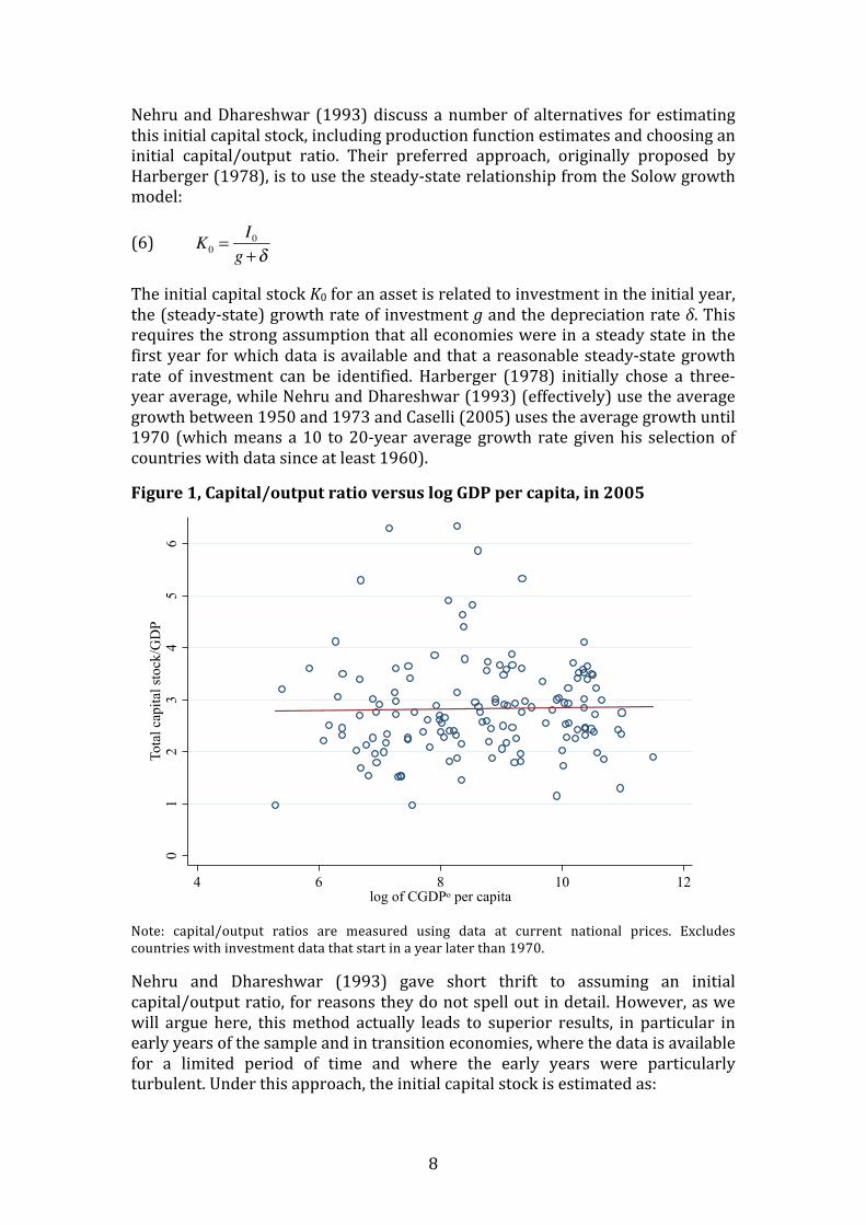
Figure 1, Capital/output ratio versus log GDP per capita, in 2005
Note: capital/output ratios are measured using data at current national prices. Excludes countries with investment data that start in a year later than 1970.
Nehru and Dhareshwar (1993) gave short thrift to assuming an initial capital/output ratio, for reasons they do not spell out in detail. However, as we will argue here, this method actually leads to superior results, in particular in early years of the sample and in transition economies, where the data is available for a limited period of time and where the early years were particularly turbulent. Under this approach, the initial capital stock is estimated as:
K0 =I0
g +δ
01
23
45
6To
tal c
apita
l sto
ck/G
DP
4 6 8 10 12log of CGDPo per capita

9
(7) K0 = Y0 × k ,
where Y0 is GDP in the initial year and k is the assumed capital/output ratio K/Y. To motivate the choice for k, Figure 1 plots capital/output ratios in 2005, where capital is summed over all assets, against GDP per capita. The figure includes the 142 countries with investment data since at least 1970. The figure shows considerable variation in capital/output ratios around a median value of 2.7. The least squares regression line indicates that there is no systematic relationship between GDP per capita and capital/output ratios.
To solidify this finding, Table 3 shows a number of regressions, aiming to explain differences in capital/output ratios with differences in GDP per capita. Note that the capital/output ratio is at current national prices, so does not reflect differences in inflation or relative prices of the capital stock versus the price of GDP. The explanatory variable is based on PWT8.0 and is measured as log CGDPo per capita, the comparative productivity capacity of each economy. Column (1) shows the regression on the data in Figure 1, so with data for 2005 and including only countries with investment data since at least 1970. Column (2) includes all countries and years and shows a similarly insignificant relationship between the GDP per capita level and the capital/output ratio.
Table 3, The relationship between capital/output ratios and GDP per capita
Note: dependent variable is the capital/output ratio, measured using data at current national prices. Robust standard errors are in parentheses; in columns (2)-‐(8), errors are clustered by country. Column (1) only includes data for 2005 for countries with investment data since at least 1970. The remaining columns include all countries and years in PWT8.0. The number of observations in column (6)-‐(8) is lower than in (2)-‐(5) because there is no data on investment in these assets for a range of countries. *** p<0.01, ** p<0.05, * p<0.1
Columns (3) through (8) analyze the separate components of the total capital stocks. For the largest component, structures, there is no significant relationship and the same is true for transport equipment. Other machinery, computers and software ratios increase with GDP per capita – a finding that is line with the findings of Comin and Hobijn (2004, 2010) – while communication equipment is less intensively used in richer countries. However, for the purpose of setting an initial capital stock, these relationships are less relevant to account for, because the asset life of machinery and communication equipment is much shorter and because the use of computers and software only became widespread since the 1960s in the US and later in other countries. Furthermore, structures account for, on average, 80 percent of the value of the capital stock, so its initial stock will have the most impact on the overall results.
(1) (2) (3) (4) (5) (6) (7) (8)2005 Total1stock Structures Machinery Transport Computers Communication Softwaresince11970 Full1sample equipment equipment
log1CGDPo/capita 0.0143 0.0453 0.00529 0.0279*** M0.00121 0.00458*** M0.0157*** 0.00663***(0.0528) (0.0425) (0.0390) (0.00912) (0.00476) (0.000716) (0.00455) (0.000714)
Constant 2.700*** 2.520*** 2.315*** 0.124 0.153*** M0.0275*** 0.214*** M0.0489***(0.486) (0.384) (0.354) (0.0788) (0.0420) (0.00637) (0.0422) (0.00628)
Observations 142 8,217 8,217 8,217 8,217 3,265 3,265 3,265RMsquared 0.000 0.002 0.000 0.029 0.000 0.150 0.039 0.322
10
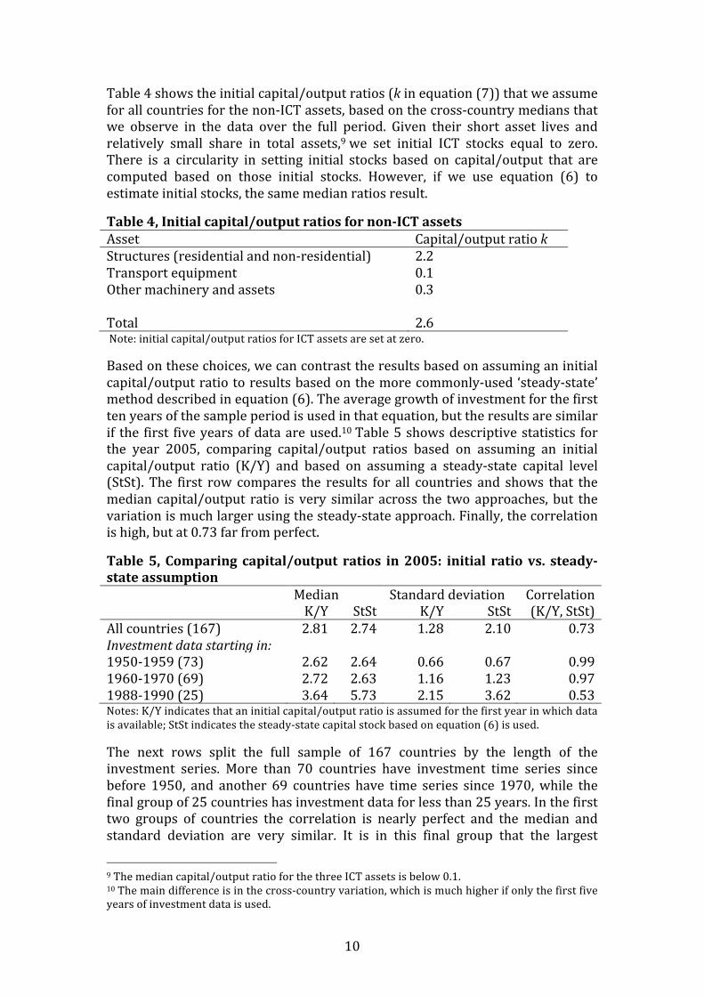
Table 4 shows the initial capital/output ratios (k in equation (7)) that we assume for all countries for the non-‐ICT assets, based on the cross-‐country medians that we observe in the data over the full period. Given their short asset lives and relatively small share in total assets,9 we set initial ICT stocks equal to zero. There is a circularity in setting initial stocks based on capital/output that are computed based on those initial stocks. However, if we use equation (6) to estimate initial stocks, the same median ratios result.
Table 4, Initial capital/output ratios for non-‐ICT assets Asset Capital/output ratio k Structures (residential and non-‐residential) 2.2 Transport equipment 0.1 Other machinery and assets 0.3 Total 2.6 Note: initial capital/output ratios for ICT assets are set at zero.
Based on these choices, we can contrast the results based on assuming an initial capital/output ratio to results based on the more commonly-‐used ‘steady-‐state’ method described in equation (6). The average growth of investment for the first ten years of the sample period is used in that equation, but the results are similar if the first five years of data are used.10 Table 5 shows descriptive statistics for the year 2005, comparing capital/output ratios based on assuming an initial capital/output ratio (K/Y) and based on assuming a steady-‐state capital level (StSt). The first row compares the results for all countries and shows that the median capital/output ratio is very similar across the two approaches, but the variation is much larger using the steady-‐state approach. Finally, the correlation is high, but at 0.73 far from perfect.
Table 5, Comparing capital/output ratios in 2005: initial ratio vs. steady-‐state assumption Median Standard deviation Correlation K/Y StSt K/Y StSt (K/Y, StSt) All countries (167) 2.81 2.74 1.28 2.10 0.73 Investment data starting in: 1950-‐1959 (73) 2.62 2.64 0.66 0.67 0.99 1960-‐1970 (69) 2.72 2.63 1.16 1.23 0.97 1988-‐1990 (25) 3.64 5.73 2.15 3.62 0.53 Notes: K/Y indicates that an initial capital/output ratio is assumed for the first year in which data is available; StSt indicates the steady-‐state capital stock based on equation (6) is used.
The next rows split the full sample of 167 countries by the length of the investment series. More than 70 countries have investment time series since before 1950, and another 69 countries have time series since 1970, while the final group of 25 countries has investment data for less than 25 years. In the first two groups of countries the correlation is nearly perfect and the median and standard deviation are very similar. It is in this final group that the largest
9 The median capital/output ratio for the three ICT assets is below 0.1. 10 The main difference is in the cross-‐country variation, which is much higher if only the first five years of investment data is used.

11
differences can be seen: the steady-‐state approach leads to a median capital/output ratio that is much higher, variation that is much higher, and the correlation between the two approaches is quite low at 0.53. The countries in this last group are nearly all countries that emerged from the former Soviet Union, Yugoslavia and Czechoslovakia. In those newly-‐formed countries, the early 1990s were anything but a steady-‐state, involving a transition to market-‐based economies. Using the steady-‐state approach implies very high capital/output ratios, especially early in the transition period. This is because these countries saw rapidly falling GDP in the first years of their transition and thus a large increase in their capital/output ratio. To illustrate, in 1995 the steady-‐state approach implies a capital/output ratio in the Czech Republic of 6.5 and in Slovakia of 8.9, while in Poland and Hungary (transition countries with longer time series), the ratios are 3.4 and 3.7. In contrast, if the assumption of initial capital/output ratio is used, the 1995 capital/output ratio in the four countries varies between 3.7 and 3.9.
Figure 2, Comparing capital/output ratios over time: initial ratio vs. steady-‐state assumption, 1970-‐2011
Notes: K/Y indicates that an initial capital/output ratio is assumed for the first year in which data is available; StSt indicates the steady-‐state capital stock based on equation (6) is used. For each year, the median, standard deviation and correlation is computed for the cross-‐section of 142 countries with investment data since 1970 or earlier.
Furthermore, Figure 2 shows that differences are much larger in earlier years. The figure shows the median capital/output ratio for the 142 countries with investment data since 1970 according to the two approaches. As the figure illustrates, from the mid-‐1980s onwards, the median capital/output ratio fluctuates between 2.5 and 3.1 according to both approaches, which suggests this is the standard range for the capital/output ratio. Assuming an initial capital/output ratio ensures that the data for these countries are continuously
1.5
22.5
3
1970 1980 1990 2000 2010
K/Y StSt
12
within this range, but applying the steady-‐state assumption implies that capital levels are much too low for a long period of time, starting at a median level of 1.9 and reaching 2.5 only in 1980. We therefore conclude that assuming the initial capital/output ratios from Table 4 ensures more plausible capital stocks across all countries and years.
Capital stocks and depreciation Given an initial capital stock K0, investment at constant prices I and depreciation rates δ, it is straightforward to compute capital stocks for asset a in country i at time t using the Perpetual Inventory Method (PIM):
(8) Kait = 1−δ a( )Kait−1 + Iait
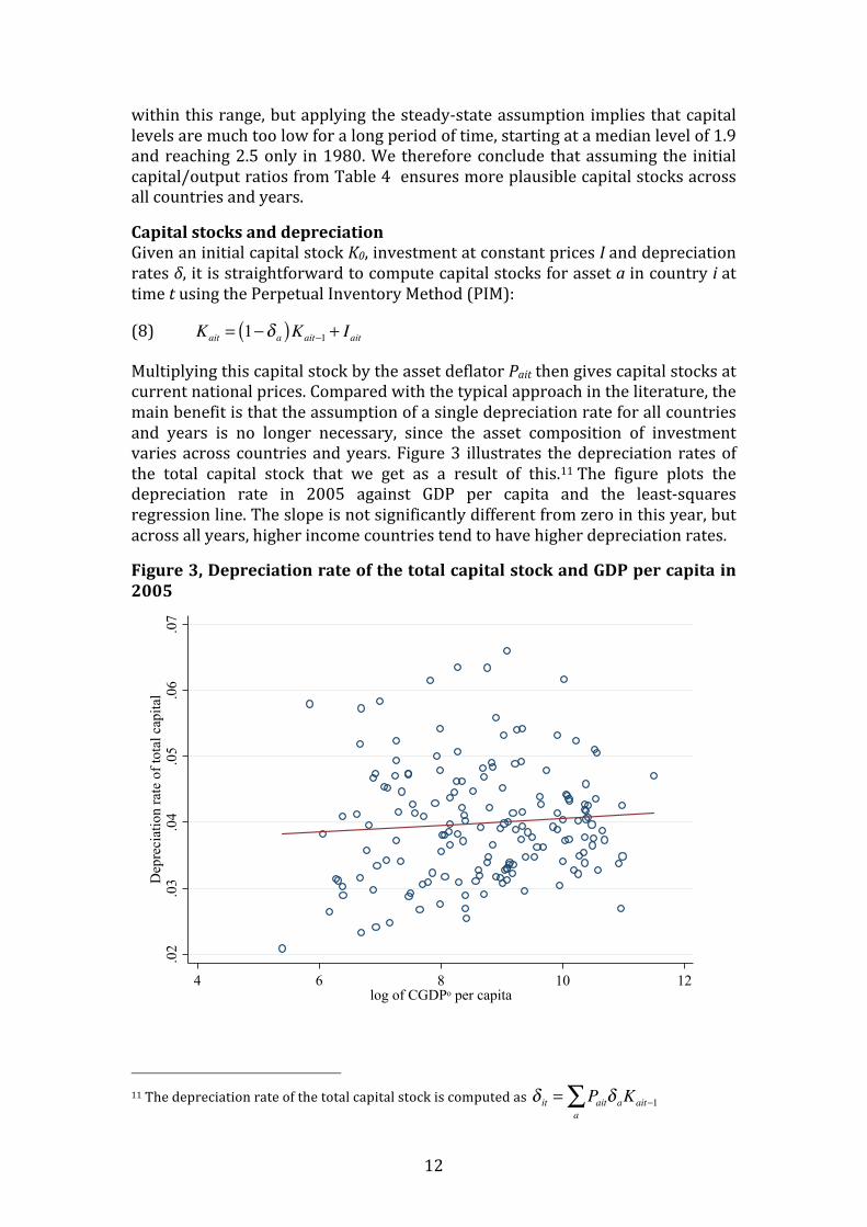
Multiplying this capital stock by the asset deflator Pait then gives capital stocks at current national prices. Compared with the typical approach in the literature, the main benefit is that the assumption of a single depreciation rate for all countries and years is no longer necessary, since the asset composition of investment varies across countries and years. Figure 3 illustrates the depreciation rates of the total capital stock that we get as a result of this.11 The figure plots the depreciation rate in 2005 against GDP per capita and the least-‐squares regression line. The slope is not significantly different from zero in this year, but across all years, higher income countries tend to have higher depreciation rates.
Figure 3, Depreciation rate of the total capital stock and GDP per capita in 2005
11 The depreciation rate of the total capital stock is computed as δ it = Paitδ aKait−1
a∑
.02
.03
.04
.05
.06
.07
Dep
reci
atio
n ra
te o
f tot
al c
apita
l
4 6 8 10 12log of CGDPo per capita
13
This fits with the finding from Table 3 that richer countries have higher capital/output ratios for assets with high depreciation rates: machinery, computers and software. So, for example, the US had a depreciation rate in 2011 of 4.1 percent, while China had a rate of 3.1 percent. Since the capital stocks of richer countries are depreciating at a more rapid rate, the capital stock levels we estimate here will be relatively lower than when comparing capital stocks estimated based on a common depreciation rate across countries. So when accounting for differences in GDP per capita based on differences in capital and labor (i.e. development accounting), the current capital stocks will account for less of cross-‐country income variation than those based on the standard approach, see Section 5.
Capital stock at constant national prices With capital stocks constructed for each of the assets, we construct a total capital stock at constant national prices, RKNA in PWT8.0. Ideally, this would be a measure of capital services, not capital stocks. A capital services measure would reflect that shorter-‐lived assets have a larger return in production, as indicated by the user cost of capital of each asset (e.g. OECD, 2009). As a result, buildings, which represent on average 80 percent of the capital stock at current prices, would represent a much lower share of capital services. However, the data requirements for estimating capital services are higher than for a capital stock measure. In particular, the user cost of capital of an asset should include, alongside the depreciation rate, a required rate of return on capital and the rate of asset price inflation. Asset-‐specific inflation rates are not available for many countries, as mentioned above, and the required rate of return on capital is generally hard to measure well (see e.g. Inklaar, 2010). Furthermore, in countries that have experienced periods of extreme inflation in the past, any measurement error in either inflation or the rate of return would lead to substantial swings in the user cost of capital. Finally, the user cost would be needed for comparisons over time but also across countries. This implies that mismeasurement of user costs in one country would affect capital input estimates for other countries as well.
We therefore use the total capital stock as our measure of capital input.12 The RKNA variable is constructed as a Törnqvist aggregate of the individual asset growth rates:
(9) Δ logRKitNA = vaitΔ logKait
a∑ ,
with vait = 12 vait−1 + vait( ) and vait = PaitKait PaitKait
a∑ . So the growth of the capital
stock at constant national prices for each assets is weighted by its two-‐period average share in the capital stock at current national prices. Equation (9) defines the growth rate of RKNA and the level in 2005 is set equal to the total capital stock at current reference prices in that year.
12 The capital stock, rather than capital services, is also the appropriate measure of the (wealth) value of assets, see OECD (2009).

14
Capital stock at current reference prices The computation of the capital stock at current reference prices involves converting the capital stock at current national prices using a PPP for the capital stock. The computation is analogous to that of the growth of the capital stock at constant prices in equation (9): the capital stock PPP is computed based on PPPs for each of the assets and the capital stocks at current national prices are used in weighting. One important difference is that rather than using capital-‐stock weights for two consecutive periods, there is no such natural ordering when comparing across countries. We therefore use the GEKS procedure, which effectively uses capital-‐stock weights of all countries in the computation:13
(10) PijK = ∏
k=1
CPikFPkj
F( )1 C , where PijF = Pi
I 'Ki
PjI 'Ki
⎛
⎝⎜⎞
⎠⎟PiI 'K j
PjI 'K j
⎛
⎝⎜⎞
⎠⎟⎡
⎣⎢⎢
⎤
⎦⎥⎥
0.5
This equation shows that the overall capital stock PPP, PK between countries i and j is a geometric average of the Fischer PPPs, PF. This geometric averaging ensures that the comparison between countries i and j directly gives the same result as when comparing i to j via country k, so-‐called transitivity. The Fischer PPPs are computed using the investment PPPs PI and the capital stocks at current national prices K.
The PPPs for each asset are based on PPP benchmark surveys: the six ICP surveys since 1970 and the more frequent surveys by the OECD and Eurostat since 1995. The PPPs from these surveys do not directly map into the six assets we use. In some surveys, there would not be sufficiently detailed data to separately distinguish each of the six assets. At a minimum, it is always possible to distinguish investment in structures from investment in machinery and equipment and usually this latter category is also split between transport equipment and other machinery. In case of missing detail, the more aggregate PPP is applied to each of the detailed assets, such as the machinery PPP for ICT assets and for other machinery. There would also sometimes be more detailed PPPs than the six we need and in those cases, we use a GEKS procedure with investments from the surveys as weights to arrive at the required six asset PPPs.
Following Feenstra et al. (2013a), benchmark PPPs are used in a given year whenever available. If instead a year is in between PPP benchmarks, we interpolate the PPP between these benchmarks. As detailed in Feenstra et al. (2013a), we take into account the pattern of inflation in the intervening years, but the estimated PPP is constrained by the benchmark observations. For observations before the first benchmark or after the last benchmark, we extrapolate the PPPs using relative asset inflation rates. While for these extrapolated observations, the change in PPPs is the same as the relative inflation rate, this will not be the case in general. As a result, the comparative capital stock level will show a different trend than the capital stock at constant national prices, see also Feenstra et al. (2013b) for a more extensive discussion of the implications of this approach.
13 See Feenstra et al. (2013a) for the use of the GEKS procedure in the broader context of PWT8.0 and further references.

15
Figure 4 provides a cross-‐country view for 2005 of the resulting relative price level of the capital stock. As Hsieh and Klenow (2007) found, the prices of investment goods in poorer countries are high relative to the price of consumption and this is confirmed for 2005 in the left panel of Figure 4. Since many investment goods are traded, their prices are relative close to the exchange rate. In contrast, a considerable part of consumption is non-‐traded and prices in the non-‐traded sector tend to be lower in poorer countries, the so-‐called Penn effect. However, structures are non-‐traded, so their prices will be more similar to consumption prices. Since the depreciation rate of structures is lower than of other assets, the weight of structures in the capital stock will be larger than in total investment. As a result, the price level of the capital stock gives greater weight to the non-‐traded part of investment than the price level of investment.14
Figure 4, The investment and capital stock price relative to the household consumption price level in 2005
Note: only countries that participated in the 2005 ICP benchmark survey are included. The price level of investment goods (left panel) and the price level of the capital stock (right panel) is divided by the price level of household consumption.
As a result, the capital stock levels in PWT8.0 will typically be higher in poorer countries than the more simplistic capital stock estimates that have been predominantly used in the literature. The reason is that those simplistic capital stocks were constructed using PWT investment series, without taking the larger weight of structures prices in the relative capital stock into account. We constructed a simplistic capital stock using the same procedure as in Caselli (2005), so cumulating PPP-‐converted investment assuming a common
14 Put differently, with increasing income, the price of investment increases slowly (regression coefficient of 0.09), while the price of capital increases at a more rapid rate (0.13) than the price of consumption (0.11).
.51
1.5
22.
5
4 6 8 10 12log of CGDPo per capita
Investment/consumption price.5
11.
52
2.5
4 6 8 10 12log of CGDPo per capita
Capital stock/consumption price

16
depreciation rate (4%, based on Figure 3). The differences in 2005 between this simplistic capital stock and the PWT8.0 capital stock are shown in Figure 5. As the figure shows, the differences are quite large and, as predicted from Figure 4, the simplistic capital stock underestimates capital input in poorer countries: the plotted regression line is highly significant and has a fairly large slope. The PWT8.0 capital stocks thus provide a clearly different view than based on earlier approaches and a view that is more closely linked to the concept it represents.15
Figure 5, The difference between the simplistic and PWT8.0 capital/output ratio in 2005
Note: simplistic capita stock cumulates overall real investment and depreciates it at a common 4 percent. PWT8.0 capital stock uses asset-‐specific investment and depreciation rates and converts to a common currency using a capital stock PPP.
4. Labor shares This section is devoted to estimating the share of labor income in GDP. This is a challenge because, in contrast to the labor income of employees, the labor income of self-‐employed workers is not directly observable. This is because their income will typically consist of compensation for both their labor supply and any capital they may own. This issue was taken up by Gollin (2002), who discusses different methods for estimating the labor compensation of self-‐employed workers. He showed for a modest set of countries that suitably adjusted labor shares are much more similar than naïve shares that ignore the labor compensation of the self-‐employed. This is because in poorer countries, more people are self-‐employed, which compensates for the lower naïve labor share in
15 A measure of relative capital services will be different yet again. Shorter-‐lived assets, like computers, have higher user costs of capital and thus a relatively larger share in capital services than in capital stocks. The precise effect is dependent on the rate of return on capital and the asset revaluation term in the various countries.
BLZBMU
CHEDMA
GNB
GRD IRLIRQSDN
SYR
TJK
TTO
UKR
USA
UZB
ZWE
-1-.5
0.5
Diff
eren
ce b
etw
een
sim
plis
tic a
nd P
WT8
.0 c
apita
l/out
put r
atio
4 6 8 10 12log of CGDPo per capita
17
poorer countries. For PWT8.0 we build upon these efforts by adding an adjustment method, increasing the range of countries, and, most importantly, extending the time period covered. Based on these, we come up with a ‘best estimate’ labor share based that is subsequently used in our TFP calculations. The end result is labor share estimates for up to 127 out of 167 countries in PWT8.0, covering the period since 1950.
Basic data and adjustment methods The starting point is National Accounts data on compensation of employees, GDP at basic prices16 and mixed income. Mixed income is the total income earned by self-‐employed workers, so it is a combination of capital and labor income. Given the aim of dividing the income of the self-‐employed between labor and capital, data on mixed income is very helpful by providing an upper bound to the amount of labor income earned by the self-‐employed.17 Indeed, two of Gollin’s (2002) adjusted labor shares rely on mixed income information. The first adjustment allocates all mixed income to labor, assuming that self-‐employed workers only use labor input. The second adjustment assumes that self-‐employed workers use labor and capital in the same proportion as the rest of the economy.
Mixed income data is available for 60 of the countries in PWT, so additional information is required. Gollin’s (2002) third additionally uses data on the number of employees and the number of self-‐employed and assumes that self-‐employed earn the same average wage as employees. These data are drawn from the ILO LABORSTA database.18 The ‘same-‐wage’ assumption may not be too far off the mark in advanced economies where the share of employees in the total number of persons engaged (employees + self-‐employed) is 85-‐95 percent. However, in many emerging economies this share is below 50 percent and as low as 4 percent.19 In those countries, using information on the wages of employees will overstate the labor income of self-‐employed.20
We therefore propose an alternative adjustment method. Most self-‐employed workers are active in agriculture. According to the Socio-‐Economic Accounts (SEA) of the World Input-‐Output Database (see Timmer, 2012), agriculture employs about half of the self-‐employed in poorer countries. The agricultural sector also uses very few fixed assets in these countries as, according to the SEA, the agricultural labor share (accounting for the labor income of self-‐employed) is over 90 percent of value added, on average. We therefore have an adjusted labor
16 Net taxes on products are excluded since this is not income accruing to any of the factor inputs but a direct transfer to government. 17 Throughout, we are taking the information from National Accounts as given. It should be noted however that there are major challenges to accurately measuring the income earned from informal sources; see e.g. Jerven (2012) for a recent discussion on the challenges of National Accounts measurement across African countries. 18 These data are supplemented by data from the Socio-‐Economic Accounts of the World Input-‐Output Database, see www.wiod.org. 19 The share of employees in persons engaged is strongly positively related to GDP per capita. 20 This is an area of active research. For example, Bargain and Kwenda (2011) find small differences in earnings, conditional on worker characteristics, in the non-‐agricultural sector in Brazil and Mexico but much lower earnings of self-‐employed in South Africa. Systematic differences in worker characteristics will lead to further differences in average (unconditional) wages.
18
share that adds all of value added in agriculture to labor compensation of employees.21 This adjustment could be too large as it ignores all income from capital and land and the labor income of employees in this sector is double-‐counted. 22 On the other hand, the labor income of self-‐employed outside agriculture is ignored.
Table 6, Descriptive statistics for the different labor share alternatives, 2005
Note: StDev: standard deviation, Obs: number of observations. Naïve share is the share of labor compensation of employees (COMP) in GDP. Adjustment 1 adds mixed income (MIX): (COMP+MIX)/GDP. Adjustment 2 assumes the same labor share for mixed income as for the rest of the economy: COMP/(GDP-‐MIX). Adjustment 3 assumes the same average wage for self-‐employed (SEMP) as for employees (EMPE): (COMP/GDP) *(EMPE+SEMP)/EMPE. Adjustment 4 adds value added in agriculture (AGRI): (COMP+AGRI)/GDP.
This provides us with data on the share of labor compensation of employees in GDP at basic prices and four adjusted shares, namely two based on mixed income, one based on the share of employees in the number of persons engaged and one based on the share of agriculture in GDP. Table 6 shows descriptive statistics for these shares in 2005. Showing statistics for a single year makes it easier to illustrate the cross-‐country variation since the basic data for some countries is much more extensive than for others and 2005 gives the largest coverage of countries.23
The table shows that, as in Gollin (2002), the naïve approach of using labor compensation of employees leads to very low labor shares of 42 percent on average and as low as 5 percent (in Nigeria). However, there are also some very high labor shares, up to 89 percent (in Bhutan). Adjustments 1 and 2 – based on mixed income data– show notably higher labor shares, though these can only be computed for 53 of the 108 countries. Especially some of the main oil-‐producing countries (Qatar, Oman, Venezuela) also show quite low labor shares (20-‐45%) based on these adjustments.
Using information on the number of self-‐employed and assuming they earn the same average wage as employees (adjustment 3) leads to average labor shares that are close to the commonly assumed labor share of 0.7 in Caselli (2005) and many others. Here too, though, there are countries with very low shares (Kuwait: 0.22), and some with unrealistically high shares, such as Bhutan (2.27). Bhutan already had a very high labor share according to the naïve share, so this overestimation is to be expected. This could indicate that, in contrast to National 21 We could have added value added in distributive trade as well, but as it has a lower labor share, we opted to only include agriculture. 22 A correction could be made in principle, but there is limited data to do this consistently across countries. 23 The sample of countries is different in each row. Descriptive statistics for the common sample of 42 countries shows very similar averages but with a notably smaller range.
Share Mean StDev Min Max ObsNaïve2share 0.42 0.14 0.05 0.89 108Adjustment21,2mixed2income 0.60 0.12 0.20 0.90 53Adjustment22,2part2mixed2income 0.53 0.13 0.18 0.73 53Adjustment23,2average2wage 0.66 0.24 0.22 2.27 74Adjustment24,2agriculture 0.51 0.14 0.17 1.13 108
19
Accounting rules, the statisticians in Bhutan have already imputed the labor income of self-‐employed in their ‘employee compensation’ numbers. Lesotho’s labor share under adjustment 3 of 2.05 indicates a similar problem.
The fourth adjustment adds the value added share of agriculture to the naïve share. The average share is somewhat lower than the commonly assumed two-‐thirds labor share but there are no countries with labor shares as extreme as under adjustment 3, though Bhutan is again the country with the highest labor share. In this broad cross-‐country setting, it would seem that any of the four adjustments would count as an improvement over the naïve share, but also that the mechanical application of one of these adjustments would not fit all countries equally well.
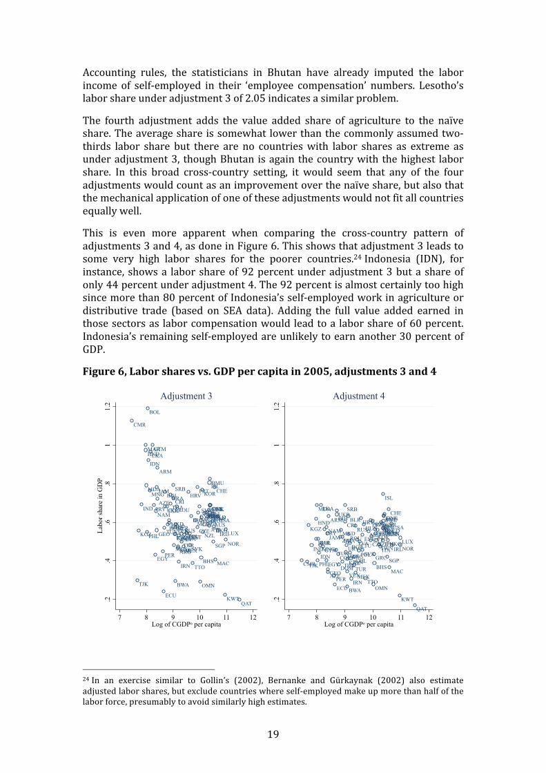
This is even more apparent when comparing the cross-‐country pattern of adjustments 3 and 4, as done in Figure 6. This shows that adjustment 3 leads to some very high labor shares for the poorer countries.24 Indonesia (IDN), for instance, shows a labor share of 92 percent under adjustment 3 but a share of only 44 percent under adjustment 4. The 92 percent is almost certainly too high since more than 80 percent of Indonesia’s self-‐employed work in agriculture or distributive trade (based on SEA data). Adding the full value added earned in those sectors as labor compensation would lead to a labor share of 60 percent. Indonesia’s remaining self-‐employed are unlikely to earn another 30 percent of GDP.
Figure 6, Labor shares vs. GDP per capita in 2005, adjustments 3 and 4
24 In an exercise similar to Gollin’s (2002), Bernanke and Gürkaynak (2002) also estimate adjusted labor shares, but exclude countries where self-‐employed make up more than half of the labor force, presumably to avoid similarly high estimates.
ARG
ARM
AUSAUT
AZE
BEL
BGR
BHS
BIH
BLR
BMU
BOL
BRA
BWA
CAN
CHE
CHL
CMR
COLCRI
CYP
CZE
DEU
DNK
DOM
ECU
EGY
ESP
EST
FINFRAGBR
GEO
GRC
GTM
HKG
HND
HRV
HUN
IDN
IND
IRL
IRN
ISL
ISRITA
JAM
JPNKAZ
KGZ
KOR
KWT
LKA
LTULUX
LVA
MAC
MAR
MDA
MEX
MKD MLT
MNG
MUS
NAM NLD
NORNZL
OMN
PAN
PER
PHL POL
PRT
PRY
QAT
ROU
RUS
SGP
SRB
SVK
SVNSWETHA
TJK
TTO
TUN
TUR
TWNUKR
URY
USA
VENZAF
.2.4
.6.8
11.
2La
bor s
hare
in G
DP
7 8 9 10 11 12Log of CGDPo per capita
Adjustment 3
ARG
ARM
AUSAUT
AZE
BEL
BGR
BHS
BIH BLR BMU
BOL BRA
BWA
CAN
CHE
CHLCMRCOL
CRI
CYPCZE
DEU
DNK
DOM
ECU
EGY
ESPEST
FINFRAGBR
GEO
GRCGTM
HKG
HND HRVHUN
IDNIND IRL
IRN
ISL
ISR
ITA
JAMJPN
KAZ
KGZKOR
KWT
LKA
LTULUXLVA
MAC
MAR
MDA
MEX
MKD MLT
MNGMUS
NAM NLD
NORNZL
OMN
PAN
PER
PHL
POL
PRTPRY
QAT
ROURUS
SGP
SRB
SVK
SVNSWE
THATJK
TTO
TUN
TUR
TWN
UKR
URY
USA
VEN
ZAF
.2.4
.6.8
11.
2
7 8 9 10 11 12Log of CGDPo per capita
Adjustment 4

20
Note: see notes to Table 6 for a description of the adjustments. Both figures include only countries for which data on adjustment 3 is available and excludes Bhutan and Lesotho (both with labor shares under adjustment 3 exceeding 2).
Best estimate labor share These results suggest that a single adjustment approach is not appropriate for all countries. We therefore construct a ‘best estimate’ labor share based on the following four rules:
1. Where available, adjustments based on mixed income seem preferable as this income directly relates to the income of self-‐employed, giving an upper-‐bound to the labor share. Adjustment 1 seems fairly extreme by assuming that self-‐employed use no capital at all, so we consider adjustment 2 to be the more plausible approach and use those labor shares if available.
2. Whenever mixed income data is available in National Accounts statistics, the naïve labor share never exceeds 0.66. So if the naïve labor share is larger than 0.7 in a particular country, it seems reasonable, like in Bhutan, that this share already includes an imputation for self-‐employed labor income. In those cases, the naïve share is used directly.
3. Given the patterns shown in Figure 6, there seems to be a greater chance of overestimating the labor share than underestimating the labor share. A conservative estimate would thus be the smaller of adjustments 3 and 4. So this is what we use if there is no mixed income data and the naïve share is below 0.7.
To ensure complete coverage over the years, we assume labor shares remain constant or we linearly interpolate if there are missing years in the middle of the sample. After these interpolations and extrapolations, we apply the three rules. Table 7 summarizes the resulting ‘best estimate’ labor shares for 2005.
Table 7, Summary statistics of the ‘best estimate’ labor share in 2005, by type of adjustment
Note: see notes to Table 6 for details on construction of the naïve and adjusted shares.
By interpolating and assuming shares constant over time, country coverage increases to 127 countries (out of 167 in PWT8.0). The resulting cross-‐country average of 0.52 is lower than Gollin’s (2002) preferred 0.7 estimate, but it shows only a somewhat larger range than his 0.34-‐0.91.25 The average is lower, which is partly related to revisions of the underlying data for mixed income. Of the 15 countries with mixed income in both Gollin’s data and here, the average ‘adjustment 2’ labor share is 68 percent in Gollin’s (2002) data and 60 percent
25 This is the range of his Table 2, not the 0.65-‐0.80 he mentions in his abstract. Only about half of his labor shares fall within the narrow 0.65-‐0.80 range.
Share #'of'countries Mean StDev Min MaxOverall 127 0.52 0.14 0.18 0.89of#which:Adjustment'2,'part'mixed'income 60 0.52 0.13 0.18 0.73Adjustment'3,'average'wage 4 0.40 0.16 0.24 0.58Adjustment'4,'agriculture 62 0.52 0.14 0.22 0.85Naïve'share 1 0.89

21
based on the current vintage of National Accounts data.26 In contrast, the naïve share and ‘adjustment 3’ share are very similar for the overlapping set of countries. In addition, there seems to be a downward trend in labor shares over time, see below for more discussion.
The table also illustrates that for almost half the countries, information on mixed income is available and therefore used. Adjustment 4 is used for most other labor share estimates and Adjustment 3 and the naïve share are only used for a few countries. The overall pattern is very similar if labor shares that are interpolated or assumed constant are dropped from the sample. The patterns shown in Table 7 for labor shares in 2005 also hold for the full sample, though there are many fewer labor shares based on observed data before the 1990s.
Table 8, Labor shares and variation across income levels and time
Note: *** p<0.01, ** p<0.05, * p<0.1. Robust standard errors, clustered by country, in parentheses. Dependent variables are the naïve share (column (1)) or the best estimate labor share. Sample excludes labor shares that are interpolated or assumed constant from other years. Oil countries are OPEC countries and those countries for which the share of energy exports exceeds one-‐third. This share was chosen as all OPEC countries have an energy export share that is at least this large.
Table 8 analyses the cross-‐country patterns in the labor share data by relating labor shares to (the log of) CGDPo per capita levels, excluding any labor shares that are assumed constant or interpolated. The naïve share in column (1) shows a strong positive relationship with GDP per capita, as Gollin (2002) also observed in his smaller sample. When using the best estimate labor share, no significant relationship with income levels is found in column (2).27 What does matter substantially is whether it is an oil country – the OPEC members and any other country in which energy exports accounts for at least one-‐third of total exports. Column (3) shows that those countries have labor shares that are on average 15 percentage points lower.
Column (4) adds a linear time trend, and this shows a significant decline in labor shares over time. This remains the case when including country dummies in column (5). In that specification, increases in income levels are even associated with lower labor shares, compared with the higher labor shares from column (1). The time trend is less steep in column (5), but still highly significant. Moreover, the pattern of declining labor shares is found across the whole sample of countries as there is a decline in the labor share in 89 of the 127 countries and
26 This compares shares for the same year as in Gollin (2002). 27 This is a finding that also holds for each of the shares based on a single adjustment, rather than the best estimate combination.
(1) (2) (3) (4) (5)Naïve-share Best-estimate Best-estimate Best-estimate Best-estimate
Log-of-CGDPo-per-capita 0.0731*** 0.00671 0.00676 0.0105 D0.0262**(0.00846) (0.00919) (0.00784) (0.00735) (0.0108)
Oil-country D0.153*** D0.146***(0.0289) (0.0264)
Time-trend D0.00334*** D0.00167***(0.000492) (0.000439)
Country-dummies no no no no yesObservations 2,975 2,237 2,237 2,237 2,237RDsquared 0.341 0.004 0.184 0.273 0.202

22
the trend is there for rich and poor countries alike.28 Finally, if year dummies rather than a linear time trend is used, the assumed linear relationship over time of Table 8 is confirmed.
The driving forces behind this broad-‐based change in labor shares over time are unclear. Blanchard (1997) also aimed to explain the decline in labor shares, but that research focused on trends in western European countries, while these developments are much more broad-‐based. The more recent work by Karabarbounis and Neiman (2013) do analyze the global decline in labor share and argue that cheaper (information and communication) capital explains much of this pattern. Regardless of the underlying cause, though, this analysis illustrates quite clearly that the standard ‘one-‐size-‐fits-‐all’ labor share of 70 percent that is commonly used in the literature is a simplification that is not supported by the facts.
5. Total factor productivity With the data on capital, labor and labor shares, we can now implement equations (2)-‐(5) and estimate comparative levels and growth of total factor productivity (TFP). The first application will be on development accounting, following Hall and Jones (1999) and Caselli (2005).29 The second application will be on growth accounting, as in Jorgenson and Vu (2010).
Development accounting Development accounting aims to assess how much of the cross-‐country differences in GDP per worker can be accounted for by observed differences in inputs. For this, the production function from equation (1) can be rewritten in per-‐worker terms as:
(11) yit = Aitkitα it hc1−α it ≡ Aitqit ,
where the lower-‐case letters refer to per-‐worker variables. Inputs of human and physical capital per worker, q, is computed as a Törnqvist index, following equation (2). Following Caselli (2005), the decomposition of the variation in GDP per worker is given by:
(12) var log yit( )( ) = var log Ait( )( ) + var log qit( )( ) + 2cov log Ait( ), log qit( )( ) . The explanatory power of observed input differences is then defined as:
(13) qsh1t =var log qit( )( )var log yit( )( ) .
To ensure that extreme outliers are not driving the results, we also compute a second success measure as the ratio between the 90th and 10th percentile of the cross-‐country distribution of GDP per worker and inputs per worker. Table 9 shows the results of the development accounting analysis. The first column uses the data for 2005 as discussed in this paper and included in PWT8.0. This shows
28 Though the trend is less steep and less significant in richer countries. 29 The main results of this analysis are also in Feenstra et al. (2013a).

23
that variation in observed inputs explains only 26 percent of the variation in GDP per worker according to success measure 1 and 22 percent according to success measure 2. The subsequent two columns show that the explanatory power is considerably lower without in particular the country-‐ and year-‐specific labor shares. Assuming a common capital share of 0.3 leads to an explanatory power of only 17 percent. Caselli (2005) also noted that his results are sensitive to the choice for the capital share, so the estimates we provide in PWT8.0 are particularly useful to put that discussion on firmer footing.
Table 9, Development accounting results
Note: top panel shows the cross-‐country variance of GDP per worker (y) and of inputs per worker (q), and qsh1, the ratio of these two. The bottom panel show the ratio of GDP per worker of the country at the 90th percentile of the cross-‐country distribution to the 10th percentile in this distribution, and qsh2, the ratio of these two. The first column shows the baseline estimates in PWT8.0 for 2005; the second column replaces the actual capital shares (measured as 1 minus the labor share) by a common 0.3. The third column also replaces the PWT capital stocks by a capital measure based on total investment and a common depreciation rate across countries and over time.
The third column replaces the capital measure developed in Section 2 by a capital measure that does not take into account variation in asset composition across countries and over time. Total investment is accumulated over time, applying a common depreciation rate of 4 percent, which is around the median depreciation rate across countries and over time since the 1980s. The explanatory power increases somewhat from the second to the third column, which is in line with findings from Figure 5 that capital stocks of poorer countries are underestimated according to the simplistic capital stock measure.
To provide the perspective over time that the new PWT8.0 data allow, Figure 7 shows the explanatory power of observed inputs, qsh1, since 1980. This starting year is chosen to cover a (broadly) similar group of countries over the full period.30 The figure indicates that the share of variation explained by observed inputs declined until about 2000, from a high of over 0.45 to a low 0.26. In terms of the variance decomposition from equation (12), this was not because the variation of observed inputs changed substantially, but rather because the variation of CGDPo per worker and the variation of TFP increased. Since 2000, the share of variation of observed has increased sharply, to 0.35. This was due, in part, to declining variation in TFP and increasing variation of observed inputs. So in summary we find that the measurement improvements made in PWT8.0 have a substantial effect on development accounting results and that the availability of 30 To be precise, the sample covers 93 countries for 1980-‐1987; 94 for 1988-‐1989, 109 for 1990-‐1991, 111 for 1992-‐1999 and 111 for 2000-‐2011.
PWT8.0 α=.3 α=.3)+)simple)Kvar(log(y)) 1.510 1.510 1.510var(log(q)) 0.398 0.262 0.289qsh1 0.26 0.17 0.19
p90/p10)y 23 23 23p90/p10)q 5 4 4qsh2 0.22 0.16 0.17

24
annual estimates of relative capital stocks and TFP shed new light on development over time.
Figure 7, Percentage of variance in CGDPo per worker explained by variation in observed inputs.
Growth accounting Just as development accounting can be used to decompose differences in the level of GDP per worker into the contribution from the level of inputs and the relative TFP level, so can growth of GDP per worker be decomposed into the sources of growth. This type of analysis goes back longer, to Solow (1957) and Jorgenson and Griliches (1967) for the US, and Jorgenson and Vu (2010) with a more recent contribution covering a global sample.
We analyze the growth in GDP per worker, decomposing this into the contribution from growth of physical capital per worker k, human capital per worker hc and TFP:
(14) Δ ln yit =α itΔ ln kit + 1−α it( )Δ lnhcit + Δ lnAit .
To illustrate the results for the sample of more than 100 countries, we compute a weighted average for each of the three elements on the right-‐hand side of equation (14) and we average over each of the three decades since 1980 (again to cover a similar group of countries over time). Figure 8 shows the result of this analysis. In the top panel, weighted average labor productivity growth for all countries with data on capital and TFP growth are included (see footnote 32), weighted by their share in ‘world’ CGDPo. This shows how the accumulation of physical capital per worker is the most important source of labor productivity growth. TFP growth plays a somewhat larger role in the 1980s and 2000s, but human capital is more important in the 1990s. Furthermore, the pace of world
.25
.3.35
.4.45
qsh 1
1980 1990 2000 2010

25
labor productivity growth has accelerated from under 2 percent on average per year in the 1980s to over 2.5 percent since 2000.
Figure 8, Global labor productivity growth and its sources, 1980-‐2011
The bottom panel splits the sample of countries in two, between those that had a level of CGDPo per capita below or above the world median in 1990. The year 1990 was chosen because data for all countries is available and data for a single year were chosen to compare the same group of countries over time. This split shows a dramatic difference, with labor productivity growth in rich countries slowing down from 1.7 to 1.2 percent per year and poor country growth increasing from 2.5 to 5.5 percent per year. Despite this great disparity in average growth pace, the importance of the different sources of growth is fairly similar across the two groups: physical capital accumulation accounts for over half of labor productivity growth in most cases. TFP growth is more important in poor countries, as might be expected because these countries still have the ‘advantage of backwardness’ and adopt technologies developed in rich countries (e.g. Keller, 2004; Griffith et al, 2004).31
6. Concluding remarks This paper has presented the new measures of inputs and productivity in PWT version 8.0. For the first time, this allows for a comparison of both the sources of income differences and the sources of economic growth for a global sample of countries covering the period since 1950. These new measures also represent important improvements on the standard approach of accounting for inputs and productivity differences in a broad cross-‐country sample (as in Caselli, 2005) and has important lessons for further work. 31 Though the results cannot be directly compared with Jorgenson and Vu (2010), the broad view of the relative importance of different sources of growth is similar to theirs.
0.5
11.
52
2.5
1980-1990 1990-2000 2000-2011World
02
46
Rich Poor1980-1990 1990-2000 2000-2011 1980-1990 1990-2000 2000-2011
Poor countries are those with a level of GDP per capita below the median in 1990
Physical capital Human capital TFP
26
Most importantly, we have demonstrated how the share of labor income in GDP differs greatly across countries and has been declining in most countries. This stands in sharp contrast to the standard assumption in the literature that the labor share is 0.7 in all countries in all years. Accounting for this heterogeneity leads to a notably different accounting for differences in income levels across countries, with observed inputs accounting for more of GDP per capita differences.
We also construct capital stocks based on investment by assets. This allows for an (average) capital depreciation rate that varies across countries and over time and for a capital stock PPP conversion factor that accounts for the difference in asset composition between investment and capital stock. Since structures have long asset lives, their share in the total capital stock is larger than in investment and thus their importance in determining the capital PPP is larger as well. This leads to systematically larger capital stocks in poorer countries than under the standard approach.
These new measure of inputs and productivity set the stage for further research and data development efforts. In measuring capital inputs, it is important to expand the range of assets to also include land, (subsoil) resources and intangible, knowledge-‐based assets. It would also be important to account for the difference in marginal costs between assets and arrive at a measure of capital services. In measuring labor inputs, accounting for differences in the quality of education rather than only the number of years of schooling would be highly relevant. But even without these improvements to the data, the current data in PWT8.0 represent an important new source for research into the sources of growth and income differences.
27
References Aghion, Phillipe and Peter Howitt (2006), “Appropriate Growth Policy: A
Unifying Framework” Journal of the European Economic Association 4(2-‐3): 269-‐314.
Bargain, Olivier and Prudence Kwenda (2011), “Earnings Structures, Informal Employment, and Self-‐Employment: New Evidence from Brazil, Mexico and South Africa” Review of Income and Wealth 57(S1): S100-‐S122.
Barro, Robert J. and Jong-‐Wha Lee (2012), “A new data set of educational attainment in the world, 1950-‐2010” Journal of Development Economics, forthcoming.
Bernanke, Ben S. and Refet S. Gürkaynak (2002), “Is Growth Exogenous? Taking Mankiw, Romer, and Weil Seriously” NBER Macroeconomics Annual 2001, MIT Press: Cambridge, MA: 11-‐71.
Blanchard, Olivier J. (1997), “The Medium Run” Brookings Papers on Economic Activity, 1997(2): 89-‐158.
Caselli, Francesco (2005), “Accounting for cross-‐country income differences” in Phillipe Aghion and Steven N. Durlauf (eds.) Handbook of Economic Growth, Volume 1A, Elsevier: 679-‐741.
Caselli, Francesco and Daniel J. Wilson (2004), “Importing Technology” Journal of Monetary Economics 51(1): 1-‐32.
Caselli, Francesco and James Feyrer (2007), “The Marginal Product of Capital” Quarterly Journal of Economics 122(2): 535-‐568.
Caves, Douglas W., Laurits R. Christensen and W. Erwin Diewert (1982a), “The Economic Theory of Index Numbers and the Measurement of Input, Output, and Productivity” Econometrica 50(6): 1392-‐414.
Caves, Douglas W., Laurits R. Christensen and W. Erwin Diewert (1982b), “Multilateral Comparisons of Output, Input, and Productivity Using Superlative Index Numbers” Economic Journal 92(365): 73-‐86.
Comin, Diego and Bart Hobijn (2004), “Cross-‐country technology adoption: making the theories face the facts” Journal of Monetary Economics 51: 39-‐83.
Comin, Diego and Bart Hobijn (2010), “An Exploration of Technology Diffusion” American Economic Review 100(5): 2031-‐2059.
Corrado, Carol, Charles R. Hulten and Daniel E. Sichel (2009), “Intangible Capital and U.S. Economic Growth” Review of Income and Wealth 55(3): 661-‐85.
De Vries, Gaaitzen, Klaas de Vries and Marcel P. Timmer (2013), “Structural Change in Africa: 1960-‐2010” GGDC Research Memorandum, no. 136 (forthcoming).
Diewert, W. Erwin and Catherine J. Morrison, 1986, “Adjusting Outputs and Productivity Indexes for Changes in the Terms of Trade” Economic Journal, 96, 659-‐679.
Feenstra, Robert C., Robert Inklaar and Marcel P. Timmer (2013a), “The Next Generation of the Penn World Table”, mimeo, available at: www.ggdc.net/pwt.
Feenstra, Robert C., Robert Inklaar and Marcel P. Timmer (2013b) “PWT8.0: a User’s Guide”, mimeo, available at: www.ggdc.net/pwt.
Fraumeni, Barbara M. (1997), “The Measurement of Depreciation in the

28
U.S. National Income and Product Accounts” Survey of Current Business, July: 7-‐23.
Gollin, Douglas (2002), “Getting Income Shares Right” Journal of Political Economy 110(2): 458-‐474.
Griffith, Rachel, Stephen Redding and John van Reenen (2004), “Mapping the Two Faces of R&D: Productivity Growth in a Panel of OECD Industries” Review of Economics and Statistics 86(4): 883-‐95.
Hall, Robert E. and Charles I. Jones (1999), "Why Do Some Countries Produce So Much More Output Per Worker Than Others?" Quarterly Journal of Economics 114(1): 83-‐116.
Hanushek, Eric A. and Ludger Woessmann (2012), “Do better schools lead to more growth? Cognitive skills, economic outcomes, and causation” Journal of Economic Growth 17(4): 267-‐321.
Harberger, Arnold (1978), “Perspectives on Capital and Technology in Less Developed Countries” in Michael J. Artis and Avelino R. Nobay (eds) Contemporary Economic Analysis, Croom Helm: London.
Hsieh, Chang-‐Tai and Peter J. Klenow (2007) “Relative Prices and Relative Prosperity” American Economic Review 97(3): 562-‐585.
Inklaar, Robert and Marcel P. Timmer (2009), “Productivity Convergence Across Industries and Countries: The Importance of Theory-‐based Measurement” Macroeconomic Dynamics 13(S2): 218-‐40.
Inklaar, Robert (2010), “The Sensitivity of Capital Services Measurement: Measure All Assets and the Cost of Capital” Review of Income and Wealth 56(2): 389-‐412.
Jerven, Morten (2012), “Comparability of GDP estimates in Sub-‐Saharan Africa: the effect of revisions in sources and methods since structural adjustment” Review of Income and Wealth, forthcoming.
Jones, Charles I. and Peter J. Klenow (2011), “Beyond GDP? Welfare across Countries and Time” available for download at http://www.stanford.edu/~chadj/rawls300.pdf.
Jorgenson, Dale W. and Zvi Griliches (1967) “The Explanation of Productivity Change” Review of Economic Studies 34(3): 249-‐83.
Jorgenson, Dale W., Frank M. Gollop and Barbara M. Fraumeni (1987), Productivity and U.S. Economic Growth Harvard Economic Studies: Cambridge, MA.
Jorgenson, Dale W. and Khuong M. Vu (2010), “Potential Growth of the World Economy” Journal of Policy Modeling 32(5): 615-‐631.
Kapiszewski, Andrzej (2006), “Arab versus Asian Migrant Workers in GCC Countries” paper for the UN Expert Group Meeting on International Migration and Development in the Arab Region, Beirut May 2006.
Karabarbounis, Loukas and Brent Neiman (2013), “The Global Decline of the Labor Share” NBER Working Paper, no. 19136.
Keller, Wolfgang (2004), “International Technology Diffusion” Journal of Economic Literature XLII: 752-‐782.
Nehru, Vikram and Ashok Dhareshwar (1993), “A new database on physical capital stock: sources, methodology and results” Revista de Analisis Economico, 8(1): 37-‐59
O’Mahony, Mary and Marcel P. Timmer (2009), “Output, Input and Productivity Measures at the Industry Level: the EU KLEMS Database”

29
Economic Journal 119(538): F374-‐403. OECD (2001) OECD Manual: Measurement of Aggregate and Industry-‐level
Productivity Growth, OECD: Paris. OECD (2009) OECD Manual: Measuring Capital, OECD: Paris. Psacharopoulos, George (1994), “Returns to investment in education: A
global update” World Development 22 (9): 1325–1343. Solow, Robert M. (1957), “Technical Change and the Aggregate Production
Function” Review of Economics and Statistics 79(3): 367-‐70. Summers, Robert and Alan Heston (1991), “The Penn World Table (Mark
5): An Expanded Set of International Comparisons, 1950–1988” Quarterly Journal of Economics, 106(2): 327–68.
World Bank (2006) Where is the Wealth of Nations? Measuring Capital for the 21st Century, World Bank: Washington DC.
30
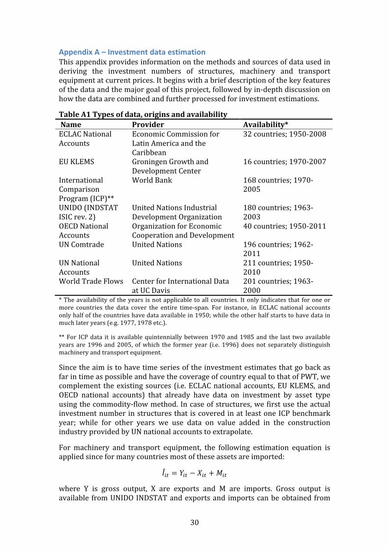
Appendix A – Investment data estimation This appendix provides information on the methods and sources of data used in deriving the investment numbers of structures, machinery and transport equipment at current prices. It begins with a brief description of the key features of the data and the major goal of this project, followed by in-‐depth discussion on how the data are combined and further processed for investment estimations.
Table A1 Types of data, origins and availability Name Provider Availability* ECLAC National Accounts
Economic Commission for Latin America and the Caribbean
32 countries; 1950-‐2008
EU KLEMS Groningen Growth and Development Center
16 countries; 1970-‐2007
International Comparison Program (ICP)**
World Bank 168 countries; 1970-‐2005
UNIDO (INDSTAT ISIC rev. 2)
United Nations Industrial Development Organization
180 countries; 1963-‐2003
OECD National Accounts
Organization for Economic Cooperation and Development
40 countries; 1950-‐2011
UN Comtrade United Nations 196 countries; 1962-‐2011
UN National Accounts
United Nations 211 countries; 1950-‐2010
World Trade Flows Center for International Data at UC Davis
201 countries; 1963-‐2000
* The availability of the years is not applicable to all countries. It only indicates that for one or more countries the data cover the entire time-‐span. For instance, in ECLAC national accounts only half of the countries have data available in 1950; while the other half starts to have data in much later years (e.g. 1977, 1978 etc.).
** For ICP data it is available quintennially between 1970 and 1985 and the last two available years are 1996 and 2005, of which the former year (i.e. 1996) does not separately distinguish machinery and transport equipment.
Since the aim is to have time series of the investment estimates that go back as far in time as possible and have the coverage of country equal to that of PWT, we complement the existing sources (i.e. ECLAC national accounts, EU KLEMS, and OECD national accounts) that already have data on investment by asset type using the commodity-‐flow method. In case of structures, we first use the actual investment number in structures that is covered in at least one ICP benchmark year; while for other years we use data on value added in the construction industry provided by UN national accounts to extrapolate.
For machinery and transport equipment, the following estimation equation is applied since for many countries most of these assets are imported:
𝐼!" = 𝑌!" − 𝑋!" +𝑀!"
where Y is gross output, X are exports and M are imports. Gross output is available from UNIDO INDSTAT and exports and imports can be obtained from

31
either United Nations Comtrade database or Feenstra’s World Trade Flows. We opt for the former source and use Feenstra’s data only in case of absence of a certain country in UN Comtrade as Comtrade information is often easier to reconcile with National Accounts data. We now turn to detailed discussion on how trade and output data are further processed to enable investment estimations.
Trade data Trade data is obtained from UN Comtrade database for the time period of 1962 to 2011 for all the countries available.32 The commodity classification codes used in downloading the data is Standard International Trade Classification (SITC) revision 1 since this classification goes furthest back in time (i.e. 1962). With SITC rev.1 at two-‐digit level we are interested in the following four codes: 71, 72, 73 and TOTAL. The sum of the first two codes is considered trade in machinery, and 73 as trade in transport equipment. TOTAL indicates the total amount of trade across all industries.
In order to have a balanced panel we first fill in the gaps that exist in the data. This requires estimating 2120 missing values, or about 10.8% of total number of observations. We apply linear interpolation, which takes the following general form:
𝑋 = 𝑋! + (𝑋! − 𝑋!)(!!!!)(!!!!!)
; 𝑀 = 𝑀! + (𝑀! −𝑀!)(!!!!)(!!!!!)
where X indicates exports, M indicates imports and the subscripts (i.e. a and b) indicate the years at which the trade data are available; t denotes year. This general approach is also followed when interpolating other data sources.
Figure A1, Share of machinery in total exports of Panama (1978-‐2005)
32 Due to the lack of data on Equatorial Guinea (GNQ) and Sao Tome and Principe (STP), we obtain the trade data of these two countries from the World Trade Flows compiled by Feenstra (2005).
0.0
05.0
1.0
15.0
2
1980 1985 1990 1995 2000 2005
Observed share Trend share (Hodrick-Prescott filter)

32
After filling in the missing values we compute the share of trade in machinery and transport equipment. These shares would frequently vary considerably from year-‐to-‐year, as is illustrated in Figure A1 for machinery exports of Panama between 1978 and 2005.
By contrast, its corresponding import share appeared to be much less volatile. To be precise, the largest exports share of machinery is about 240 times larger than its smallest share; whereas for imports share, this factor is around merely 2.12. In order to remove those undesirable spikes, Hodrick-‐Prescott (HP) time-‐series filtering technique is applied. Although the rule of thumb is to apply the smoothing parameter λ=6.25 for annual data, we used λ=1600 instead to obtain a more sensitive detector of outliers by allowing for a much smoother trend. We consider observations that have the cyclical components in the top and bottom five percentiles as outliers. Whenever the cyclical components exceed |5%| for imports and |3%| for exports they are considered as outliers whose values are then replaced by the product of their (HP generated) trend shares and total imports or exports.
In addition, in order to accomplish the goal of having time series that go as far back as possible we extrapolate the trade data all the way back to 1950 using data on gross capital formation (GCF) provided by UN national accounts.33 That is:
𝑋!"!! = 𝑋!" ∗(!"#!")!!!(!"#!")!
; 𝑀!"!! = 𝑀!" ∗(!"#!")!!!(!"#!")!
where I indexes asset type, namely machinery and transport equipment; t denotes year.
Output data For production we rely on the data provided by United Nations Industrial Development Organization (UNIDO) compiled in 2006. In this data set the commodity classification codes used is International Standard Industry Classification (ISIC) revision 2 at three-‐digit level. The following five codes are of interest to us: 300, 382, 383, 384, and 385. The first code (i.e. 300) denotes the total output value of the manufacturing industry, 384 is the output value of transport equipment, and 382+383+385 gives the output of machinery. Similar to the trade data, we first fill-‐in gaps in each country series by interpolation. Before the first and after the last observation, we keep the share of both industries in total manufacturing constant and we use the trend in UNIDO manufacturing output or National Accounts value added to come up with a balanced panel. We apply the same filtering technique as used in the trade data to correct for spikes in output.
For estimating investment in structures, we use value added in construction from the UN National Accounts. As these series also exhibit spikes, the HP filtering technique is again applied to detect the abnormal jumps. We consider observations that are in the top and bottom five percentiles as outliers.
33 Not all countries have data on gross capital formation back to 1950, thus trade data is extrapolated backwards only for those that have such data available in UN national accounts.

33
Whenever the cyclical components exceed |10%| the values are replaced by the product of their (HP generated) trend shares and GFCFNA. Calculating investment for machinery and transport equipment With data on trade and output, we apply the commodity flow method to compute investment series by asset type (i.e. machinery and transport equipment) with the following equation:
𝐼!" = 𝑌!" − 𝑋!" +𝑀!"
Since machinery and transport equipment are generally considered high-‐tech products, it is very likely that the least-‐developed countries do not produce but mostly import them from other countries. Thus, output Y is set to zero whenever the country-‐industry pair under concern has missing data for the entire time period. ne exception to note is Belarus, which has its exports volume consistently larger than that of imports. We resort to using the shares of the Russian data combined with Belarus’s own number of value added in manufacturing (i.e. DNA) as a crude measure to derive output of machinery and transport equipment manufacturing for Belarus.
In less than 0.2 percent of the cases we find negative investment estimations and these negative values are either due to a small import share or large export share. In the former case, we applied the mean share of their imports to correct for the small values of imports; while in the latter case, we replace the exports value to missing and then interpolate the values in between. Though these correction measures are rather crude, it helps to get rid of the negative investment values and yield somewhat more plausible numbers.
Benchmarking investment shares The commodity flow method (CFM) gives us estimated investment in machinery and transport equipment based on output and trade data and estimated investment in structures based on value added in construction. However, these do not provide a reliable level of investment since, for instance, a considerable part of transport equipment is used by households rather than firms. We therefore use the ICP investment data, which sums to total investment.34 Between ICP benchmark years, we use the trends in CFM-‐estimated investment to interpolate. Before the first and after the last ICP benchmark, we use CFM-‐estimated investment to extrapolate.
Especially the extrapolation procedure can lead to implausible results. For example, we find in some cases that estimated investment in structures exceeds total investment. Although the earlier filtering technique helped to mitigate this problem, we additionally set value added in construction to missing whenever structure shares exceed unity, and then interpolate or extrapolate. This does not help to fully solve the problem but the number of cases with structure share exceeding unity reduced sizably by more than two-‐thirds. In order to stay as close as possible to the original data we leave the other unsolved large structure shares as they are.
34 The ICP figures are based on older National Accounts, so we normalize total ICP investment tot National Accounts investment.

34
Combing structure, machinery and transport equipment shares We next sum the investment shares for each of the three assets. Ideally, we would want these to sum to one but this is typically not the case, so we rescale the asset shares to sum to one. For illustration purposes, consider Azerbaijan. In 1991, Azerbaijan has the most implausible estimations. Its structure share is estimated at 1.166, machinery share at 1.737 and transport equipment share at 0.134. Thus, the sum of these three shares is equal to 3.037. To rescale it back to unity, the structure share is calculated as 1.166 divide by 3.037 (38.4%). Analogously, machinery share is 57.2%, and the residual is the transport equipment share (4.4%). The following table compares the estimated shares of Azerbaijan in its worst year (i.e. 1991) with the benchmark numbers from ICP (i.e. 2005). The values undoubtedly differ, but such a rescaling already does a very decent job as the proportion of each share is in the ‘right’ order (i.e. machinery accounts for the largest share, followed by structure and transport equipment).
Table A2 Comparison of the distribution of the asset type shares of Azerbaijan
1991 2005 Structure 38.4% 43.2% Machinery 57.2% 46.3% Transport equipment 4.4% 10.5%
Integrating data from different sources To obtain a complete list of investment shares by asset type we integrate the data from different sources. As shown in table 5, we start with OECD national accounts data and complement that with EU KLEMS, which is further complemented by ECLAC and commodity-‐flow data.
Table A3 Integration of the data Order of integration Source 1 OECD NA extrapolate using 2 EU KLEMS extrapolate using 3 ECLAC extrapolate using 4 ICP/CFM ECLAC only identifies investment in structures and machinery and transport equipment combined. In order to isolate machinery from transport equipment we use the same trend for each of the two detailed assets.
Investment at current prices by asset Having computed the shares of three assets, we multiple them with total gross fixed capital formation denominated in current prices. That is:
𝐼!" = 𝑆!" ∗ 𝐺𝐹𝐶𝐹!"
where I denotes investment and S denotes share; subscripts i denotes asset type (i.e. structure, machinery, and transport equipment), and t denotes year. These are the investment series that are then used in estimation capital stocks.

35
Appendix B – Employment and human capital
Employment data For the employment series in PWT8.0, we aim to measure the total number of persons engaged in a productive activity within the boundaries of the System of National Accounts. This should include all employees, but also self-‐employed workers, unpaid family workers that are economically engaged, apprentices and the military. Since PWT’s output measure is gross domestic product, the employment measure should cover all people that work (i.e. perform a productive activity) within the boundaries of a country, regardless of nationality. This distinction is particularly relevant for countries with a large migratory workforce. For example, many Gulf states attract considerable numbers of (Asian) migrant workers35 and their employment should be included.
However, widely-‐accepted estimates of employment are not available for most countries and the basic source material – labor force surveys, establishment surveys and population censuses – is often not well-‐suited to compiling a continuous and consistent time series, with differences in coverage and definitions across surveys and over time. In a growing number of countries,36 statisticians are combining data from different sources to include a measure of employment in the National Accounts, but of those 74, data for 9 countries cover less than 10 years and in only 30 countries is the official time series 20 years or longer. In contrast, GDP data are available for up to 200 countries since 1950.37,38
We therefore combine data from various sources to estimate employment series. As our starting point, we use employment data from The Total Economy Database™ (TED) compiled by The Conference Board.39 Building on the work of Angus Maddison, they have gone to considerable lengths to derive consistent time series from a variety of sources for 123 countries. Of those, 120 are covered in PWT8.0 and we use those series as given.40 To increase coverage, we use ILO employment data (Table 2A of the LABORSTA database and, for more recent years from the ILOSTAT database) and data on employment and the labor force from the World Development Indicators (WDI) of the World Bank. This allows us to estimate employment levels for all but one of the countries in PWT.41 For all but four countries, the time series are at least 22 years long and for 30 countries, there is a continuous time series since 1950 (i.e. 62 years).
35 See e.g. Kapiszewski (2006). As detailed in this study, such migratory flows are challenging for estimating both employment and population data. 36 Combining the UN Official Country Data with OECD National Accounts yields time series of employment for 74 countries. 37 Or later if the country came into existence at a later date. 38 But not all observations for all years are equally reliable, with sometimes very large revisions, see e.g. Feenstra et al. (2013b). 39 See http://www.conference-‐board.org/data/economydatabase/ for data and descriptions of the sources. For PWT8.0, the January 2013 version of the database if used. 40 For the 1950s, some countries do not have annual series, but only 1950 values. We linearly interpolate the employment/population ratio for those years. 41 The missing country is St. Kitts and Nevis and data are dropped because during the short period for which there are labor force surveys from ILO, the implied employment/population ratio fluctuates widely, casting doubts on the reliability of these numbers.

36
We follow the approach taken for the TED and use labor force data for countries in Africa and the Middle East. This is a decidedly imperfect approach as the labor force includes both employed and unemployed. However, both WDI and ILO tend to frequently show employment figures that are larger than the labor force, casting doubt on the reliability of the employment data. But by using labor force data, employment figures for these two regions will have an upward bias. For all other countries, we first use employment estimates from ILO (possibly interpolated between survey observations), then employment estimates from WDI and finally labor force data from WDI. For example, in 2005 this means there is data from TED for 120 countries, from ILO for 16, employment data from WDI for 2 and labor force data from WDI for 26, for a grand total of 164 countries. For countries where more than one source is used, the sources are spliced together in overlapping years. This follows the same order of precedence, so the ILO level may be extrapolated using changes in the labor force from WDI.
Table B1, Employment as a share of the total and working-‐age population, mean and standard deviation by region Employment as: % of population % of working-‐age pop. mean st. deviation Mean st. deviation All countries 0.39 0.08 0.66 0.13 Asia 0.40 0.08 0.66 0.11 Europe 0.44 0.07 0.66 0.12 Latin America 0.35 0.07 0.59 0.08 Middle East & North Africa 0.31 0.09 0.54 0.09 North America 0.39 0.08 0.64 0.07 Sub-‐Saharan Africa 0.39 0.07 0.75 0.14
To illustrate some of the features of the employment data, Table B1 compares employment to the total population and to the working-‐age population (WAP)42 for a number of regions. As a share of the WAP, employment levels are broadly similar across Asia, Europe and North America, relatively low in Latin America and the Middle East and North Africa and relatively high in Sub-‐Saharan Africa. As discussed above, the employment levels for the Middle East and North Africa and Sub-‐Saharan Africa are biased upwards and this is confirmed based on data for 11 countries in Sub-‐Saharan Africa from de Vries and de Vries and Timmer (2013). Their employment data are based on a rigorous analysis of population census and labor force surveys to ensure consistent and complete coverage of all persons engaged. These 11 countries also show a 0.75 employment/WAP ratio based on PWT employment data, but an employment/WAP ratio of only 0.67 based on the Timmer et al. (2013) data. It is an open question whether employment levels in the Middle East and North Africa are even lower than the current figures suggest. Incorporating and expanding actual employment data for these regions would be an important improvement of the PWT employment series in the future.
Beyond this, the table illustrates some of the demographic differences, with Europe showing relatively high employment/population ratios, while the
42 Working-‐age population is the population between ages 15 and 64 and data are from WDI.
37
employment/WAP ratio is fairly typical. This reflects the relatively small young population, compared to younger regions such as Sub-‐Saharan Africa.
Our primary measure for the quantity of labor input is the number of workers, but ideally we should also account for differences in the average number of hours worked per person. However, data on the average number of hours worked is even harder to collect on a comparable basis than the number of workers. From the Total Economy Database™, we include in PWT8.0 data on average hours worked in 52 countries. Variation in the average number of hours worked is quite substantial and as a country’s CGDPo per capita level increases by 1 percent, the average number of hours worked significantly decreases, by 0.10 percent on average. This is relevant for productivity analysis but also from a welfare point of view, as discussed in more detail in Jones and Klenow (2011).
Human capital In measuring inputs and productivity, the aim is not to compare differences in the number of workers in a country, but rather differences in the amount of labor services, see for instance Jorgenson, Gollop and Fraumeni (1987). Workers with different amounts of human capital will have different marginal products and in a broad sense, this will depend on a worker’s innate talent and the amount and quality of formal schooling, on-‐the-‐job training and experience. In practice, the amount of human capital can be approximated by a limited number of observable characteristics, primarily the amount of formal schooling. The quality of education, as reflected in internationally comparable test scores, is also increasingly flagged as an important dimension of human capital (Hanushek and Woessman, 2012; Caselli, 2005). However, given its broad coverage of countries and years, the average years of schooling remains the most useful measure of human capital.
We draw on the database of Barro and Lee (2012), specifically version 1.3 of their data covering the 1950-‐2010 period, which includes data for 134 of the countries in PWT8.0. We follow the broader literature and let human capital hc of country i at time t be a function of the average years of schooling s:
(15) .
We use the average years of schooling for the population aged 15 and older. In some studies (Hall and Jones, 1999; Caselli, 2005), schooling of the over-‐25 population is used, which is defensible as part of the population in the 15 to 25 age range will still be in school and thus not contributing to GDP. On the other hand, the working-‐age population is between ages 15 and 64, so excluding the 15-‐25 years-‐old likely understates the amount of human capital (assuming that the years of schooling is increasing over time). To weigh the bias from excluding the 15-‐25 years-‐old category, it is helpful to consider how many are likely to still be in school in those years. According to UNESCO statistics, primary education starts between the age of 5 and 7 all over the world so students turn 15 after 8 to 10 years of schooling. Table B2 shows the fraction of countries with an average of at least 8 years and 10 years of schooling in three of the years covered by Barro and Lee (2012). This table indicates that in a growing share of countries,
hcit = eφ sit( )
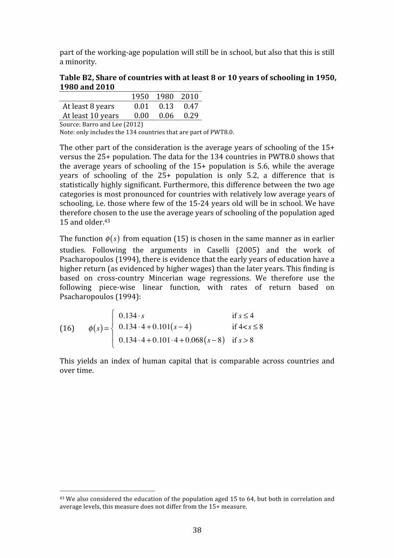
38
part of the working-‐age population will still be in school, but also that this is still a minority.
Table B2, Share of countries with at least 8 or 10 years of schooling in 1950, 1980 and 2010 1950 1980 2010 At least 8 years 0.01 0.13 0.47 At least 10 years 0.00 0.06 0.29 Source: Barro and Lee (2012) Note: only includes the 134 countries that are part of PWT8.0.
The other part of the consideration is the average years of schooling of the 15+ versus the 25+ population. The data for the 134 countries in PWT8.0 shows that the average years of schooling of the 15+ population is 5.6, while the average years of schooling of the 25+ population is only 5.2, a difference that is statistically highly significant. Furthermore, this difference between the two age categories is most pronounced for countries with relatively low average years of schooling, i.e. those where few of the 15-‐24 years old will be in school. We have therefore chosen to the use the average years of schooling of the population aged 15 and older.43
The function from equation (15) is chosen in the same manner as in earlier studies. Following the arguments in Caselli (2005) and the work of Psacharopoulos (1994), there is evidence that the early years of education have a higher return (as evidenced by higher wages) than the later years. This finding is based on cross-‐country Mincerian wage regressions. We therefore use the following piece-‐wise linear function, with rates of return based on Psacharopoulos (1994):
(16) φ s( ) =0.134 ⋅ s if s ≤ 40.134 ⋅4 + 0.101 s − 4( ) if 4< s ≤ 8
0.134 ⋅4 + 0.101⋅4 + 0.068 s − 8( ) if s > 8
⎧
⎨⎪
⎩⎪
This yields an index of human capital that is comparable across countries and over time.
43 We also considered the education of the population aged 15 to 64, but both in correlation and average levels, this measure does not differ from the 15+ measure.
φ s( )