Applied Mathematics and Computation 183 (2006) 1410–1421

www.elsevier.com/locate/amc

Designing an efficient method for tandem AGV networkdesign problem using tabu search

Gilbert Laporte a, Reza Zanjirani Farahani b,*, Elnaz Miandoabchi b,c

a Canada Research Chair in Distribution Management and GERAD, HEC Montreal,

3000 chemin de la Cote-Sainte-Catherine, Montreal, Canada H3T 2A7b Department of Industrial Engineering, Amir Kabir University of Technology, Tehran, Iran

c Supply Chain Management Research Group, Tehran, Iran

Abstract

A tandem AGV configuration connects all cells of a manufacturing area by means of non-overlapping, single-vehicleclosed loops. Each loop has at least one additional P/D station, provided as interface between adjacent loops. This studydescribes the development of a tabu search algorithm for the design of tandem AGV systems. Starting from an initial par-tition generated by a k-means clustering method, the tabu search algorithm partitions the stations into loops by minimizingthe maximum workload of the system, without allowing the paths of loops to cross each other. The new algorithm and thepartitioning algorithm presented by Bozer and Srinivasan are compared on, randomly generated problems. Results showthat in large scale problems, the partitioning algorithm often leads to infeasible configurations with crossed loops in spiteof its shorter running time. However the newly developed algorithm avoids infeasible configurations and often yields betterobjective function values.� 2006 Elsevier Inc. All rights reserved.

Keywords: AGV; Tandem configuration; Tabu search

1. Introduction

The design of handling systems is one of the most important decisions in facility design activities. Materialhandling operations cover nearly 20–50% of the overall operational costs [40]. An automated guided vehicle(AGV) is a driverless vehicle used for the transportation of goods and materials within a production plantpartitioned into cells (or departments), usually by following a wire guide-path. One of the most importantissues in designing AGV systems is the guide-path design. The problem of guide-path design for AGVs isnot new. A number of algorithms for AGV guide-path design have been developed over the past 20 years[2]. The AGV guide-path configurations discussed in previous research include Conventional/Traditional

0096-3003/$ - see front matter � 2006 Elsevier Inc. All rights reserved.

doi:10.1016/j.amc.2006.05.149

* Corresponding author.E-mail address: farahan@aut.ac.ir (R.Z. Farahani).

G. Laporte et al. / Applied Mathematics and Computation 183 (2006) 1410–1421 1411

[17,18,22,41,33,25,32,38,15,14,21,24], Tandem [8,9,27], Single loop [39,34,5,26,4,3,13,12], bi-directional shortest

path [23,11,28] and segmented flow [35–37,6].The tandem configuration, which is the concern of this paper, was introduced by Bozer and Srinivasan [7,8]

and is based on the ‘‘divide-and-conquer’’ principle. A tandem configuration is obtained by partitioning all theworkstations into single-vehicle, non-overlapping zones. Additional pick-up/delivery (P/D) points are pro-vided between adjacent zones to serve as transfer points. This configuration offers some advantages such asthe elimination of blocking and congestion, simplicity of control, and flexibility due to system modularity.It also has some disadvantages including the need for handling a load by two or more vehicles and thus longerload movement times, extra floor space and cost requirements, resulting from the use of additional P/D pointsand conveyors.

There are relatively few papers published on tandem AGV systems compared with the number of publica-tions on other systems. These studies have focused on the design of routes, routing and control of AGVs, per-formance comparison with conventional systems and modeling by Petri nets. Our literature review mostlycovers route design.

Tandem paths initially were initially proposed by Bozer and Srinivasan [7,8] who presented an analyticalmodel to compute the workload of a single loop. They developed a heuristic method for the partitioningthe stations in loops [9]. Hsieh and Sha [19] proposed a design process for the concurrent design ofmachine layout and tandem routes. Aarab et al. [1] used hierarchical clustering and tabu search to determinetandem routes in a block layout. Yu and Egbelu [43] presented a heuristic partitioning algorithm for atandem AGV system, based on the concept of variable path routing. Later Bozer and Lee [10] consideredeliminating the conveyers by using an existing station as a transfer point. Ventura and Lee [42] studied tan-dem configurations with the possibility of using more than one AGV in the loops. Huang [20] proposed anew design concept of tandem AGV based on using of a transportation center to link the transfer points inloops.

To test the viability of tandem configurations, Farling et al. [16] have performed a simulation study to eval-uate the impact of system size, machine failure rate and unload/load time on the performance of three AGVconfigurations, namely traditional (parallel unidirectional flows), the tandem flow-path and the tandem loop.In a tandem loop flow-path there exists an express loop which connects each loop see [30]. The authors con-clude that traditional layouts perform better in small systems, and tandem loop configurations perform betterin large systems.

As can be seen, most previous studies have proposed heuristic algorithms for the design of tandem routes,and only in one of the papers [1] tabu search (TS) has only been used as a subroutine in designing tandemconfigurations. Thus, the application of this metaheuristic as an overall designing process in tandem systemshas not yet been considered.

The aim of this paper is to develop a TS algorithm for the design of routes in a tandem configuration. Givena grid layout, a route sheet and the number of designed loops as inputs, the problem is to assign workstationsto loops without allowing any overlap among loops, the maximum workload of the system is minimized. Theproposed algorithm will be compared to the partitioning heuristic algorithm of Bozer and Srinivasan [9],referred to as the base algorithm, using randomly generated test problems. This paper is organized as follows.A brief description of the problem and its assumptions are presented in Section 1. The TS algorithm and itscharacteristics are discussed in Section 3, and Section 4 reports computational results. Conclusions and guide-lines to future work are presented in Section 5.

2. Problem definition

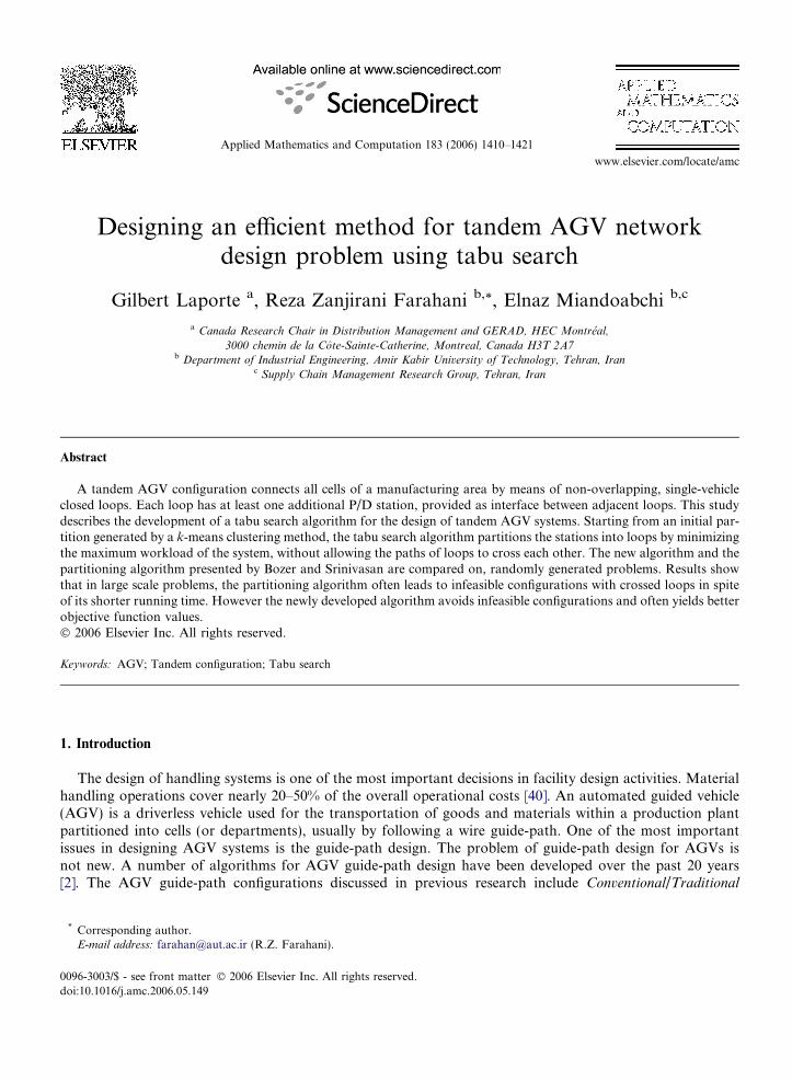
Tandem AGV systems were first introduced by Bozer and Srinivasan [7,8]. Although the tandem configu-ration can be used both in warehousing and manufacturing, it was mainly defined and developed for the lattercase. The system proposed by Bozer and Srinivasan [9] is defined on a grid layout (Fig. 1). Each workstation ispresented as a single point and may represent a machine, or a group of machines, such as a cell or adepartment.

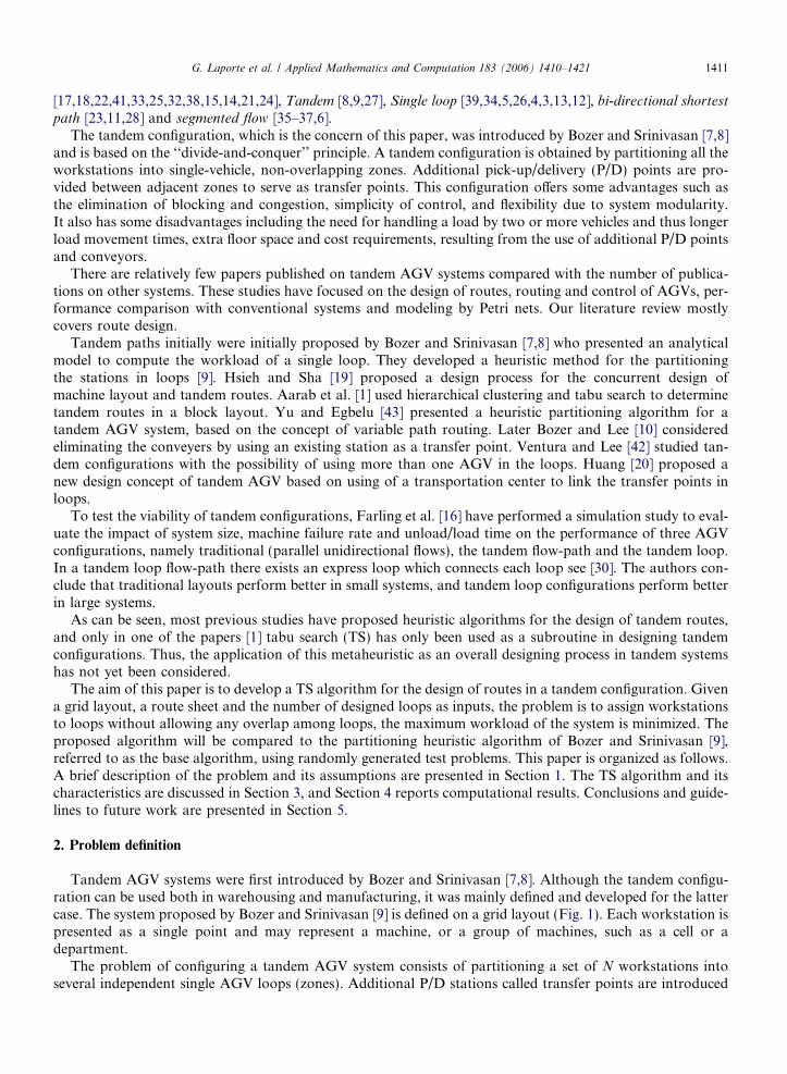
The problem of configuring a tandem AGV system consists of partitioning a set of N workstations intoseveral independent single AGV loops (zones). Additional P/D stations called transfer points are introduced

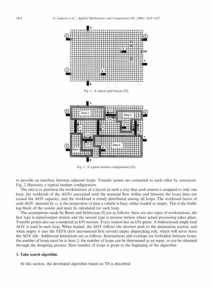
Fig. 1. A typical grid layout ([9]).

Fig. 2. A typical tandem configuration ([9]).

1412 G. Laporte et al. / Applied Mathematics and Computation 183 (2006) 1410–1421

to provide an interface between adjacent loops. Transfer points are connected to each other by conveyors.Fig. 2 illustrates a typical tandem configuration.

The aim is to partition the workstations of a layout in such a way that each station is assigned to only oneloop, the workload of the AGVs associated with the material flow within and between the loops does notexceed the AGV capacity, and the workload is evenly distributed among all loops. The workload factor ofeach AGV, denoted by x, is the proportion of time a vehicle is busy, either loaded or empty. This is the build-ing block of the system and must be calculated for each loop.

The assumptions made by Bozer and Srinivasan [9] are as follows: there are two types of workstations, thefirst type is input/output station and the second type is process station where actual processing takes place.Transfer points also are considered as I/O stations. Every station has an I/O queue. A bidirectional single loadAGV is used in each loop. When loaded, the AGV follows the shortest path to the destination station, andwhen empty it uses the FEFS (first encountered first served) empty dispatching rule, which will never leavethe AGV idle. Additional limitations are as follows. Intersections and overlaps are forbidden between loops;the number of loops must be at least 2; the number of loops can be determined as an input, or can be obtainedthrough the designing process. Here number of loops is given at the beginning of the algorithm.

3. Tabu search algorithm

In this section, the developed algorithm based on TS is described.

2

1

4

3

5

6

7

8

910

12

1714

15

16

1311

18 29

2528

27

2321

22

24

19

20

3448

454135

3849

47

4348

36

37

3240 42

4450

26 31

30

3339

Fig. 3. A typical infeasible solution.

G. Laporte et al. / Applied Mathematics and Computation 183 (2006) 1410–1421 1413

3.1. Feasibility conditions

A solution is called feasible if (1) no overlap or intersection exists among loops, (2) each station is assignedonly to one loop, and (3) the workloads are less than 1 (or a reasonable value less than 1).

The algorithm proposed by Bozer and Srinivasan [9], does not have a specific mechanism to check the over-laps among the loops. The TS algorithm checks the intersection of loops for every move. For the sake of sim-plicity, the initial routes of loops are considered as the Euclidean traveling salesman route of the stations in theloop. Fig. 3 shows a typical infeasibility in the presence of overlapping loops.

3.2. Neighborhood structure

The neighborhood of a solution is simply obtained by removing a station from one loop and adding itto another one, provided that it does not create intersection and the workload of loops does not exceed 1.A current solution corresponding to a partition of the set of workstations in L loops can be represented asfollows:

S ¼ fP 1; . . . ; P i; . . . ; P Lg; i ¼ 1; . . . ; L: ð1Þ

Consider the station s from the set of stations in loop Pi, where st 2 Pi. Also consider solution S 0 in the

neighborhood of solution S:

S0 ¼ P 01; . . . ; P 0i; . . . P 0L� �

; i ¼ 1; . . . ; L: ð2Þ

Solution S 0 is obtained by moving station s from loop Pi to loop Pj in solution S. In other words,

P 0i ¼ P i � fsg; ð3ÞP 0j ¼ P j [ fsg; j 6¼ i: ð4Þ

The feasible move mij is characterized by the transmission of station s from loop i to loop j, subject to theworkload constraint. The neighborhood of S is the set of all feasible solutions that can be reached from S

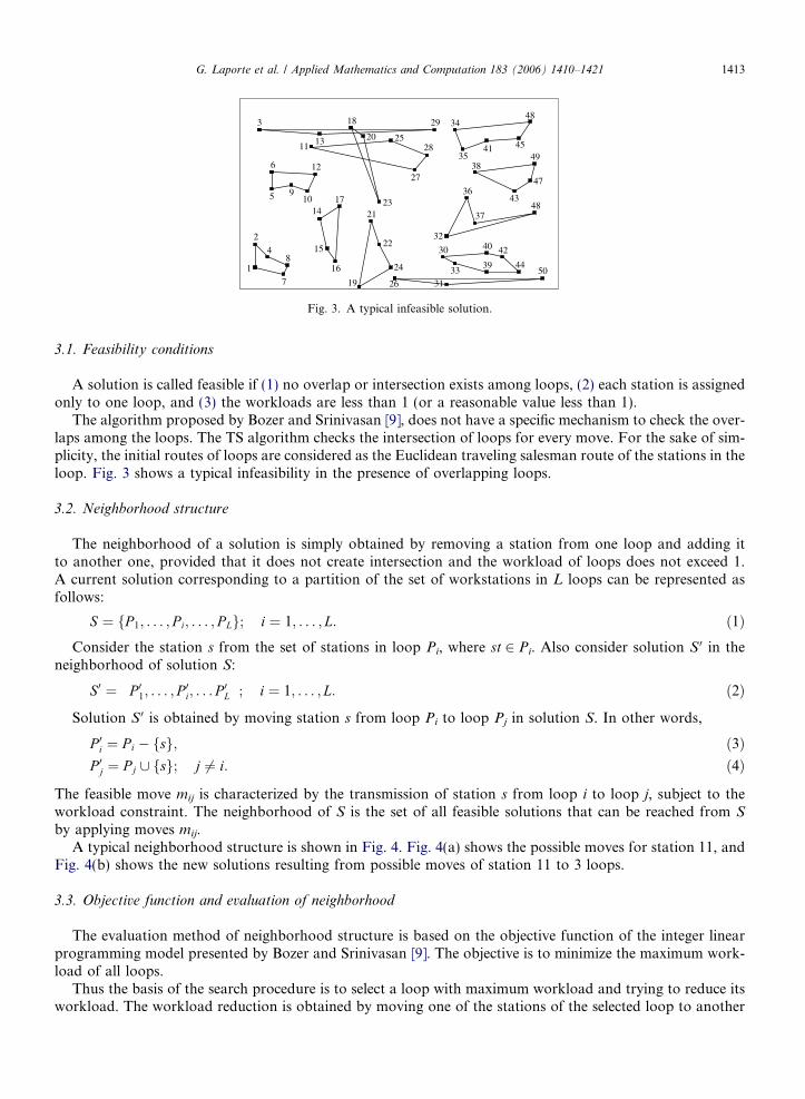
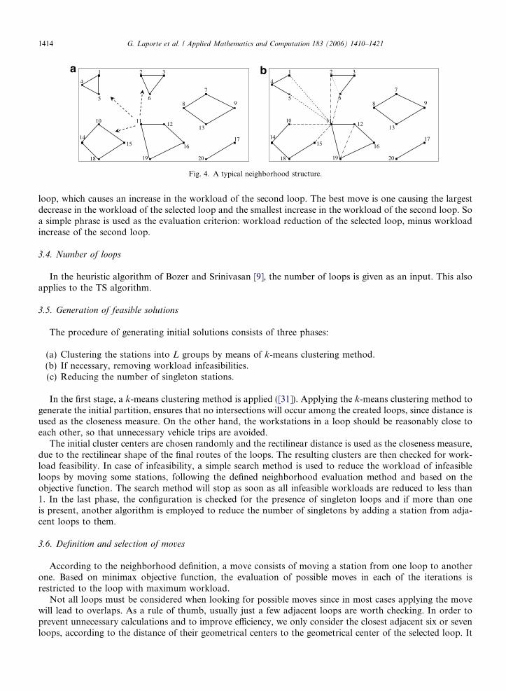
by applying moves mij.A typical neighborhood structure is shown in Fig. 4. Fig. 4(a) shows the possible moves for station 11, and

Fig. 4(b) shows the new solutions resulting from possible moves of station 11 to 3 loops.

3.3. Objective function and evaluation of neighborhood

The evaluation method of neighborhood structure is based on the objective function of the integer linearprogramming model presented by Bozer and Srinivasan [9]. The objective is to minimize the maximum work-load of all loops.

Thus the basis of the search procedure is to select a loop with maximum workload and trying to reduce itsworkload. The workload reduction is obtained by moving one of the stations of the selected loop to another

a b 1

5

4

2 3

6

7

8

13

9

16

1211

19

15

10

14

18 20

17

1

5

4

2 3

6

7

8

13

9

16

1211

19

15

10

14

18 20

17

Fig. 4. A typical neighborhood structure.

1414 G. Laporte et al. / Applied Mathematics and Computation 183 (2006) 1410–1421

loop, which causes an increase in the workload of the second loop. The best move is one causing the largestdecrease in the workload of the selected loop and the smallest increase in the workload of the second loop. Soa simple phrase is used as the evaluation criterion: workload reduction of the selected loop, minus workloadincrease of the second loop.

3.4. Number of loops

In the heuristic algorithm of Bozer and Srinivasan [9], the number of loops is given as an input. This alsoapplies to the TS algorithm.

3.5. Generation of feasible solutions

The procedure of generating initial solutions consists of three phases:

(a) Clustering the stations into L groups by means of k-means clustering method.(b) If necessary, removing workload infeasibilities.(c) Reducing the number of singleton stations.

In the first stage, a k-means clustering method is applied ([31]). Applying the k-means clustering method togenerate the initial partition, ensures that no intersections will occur among the created loops, since distance isused as the closeness measure. On the other hand, the workstations in a loop should be reasonably close toeach other, so that unnecessary vehicle trips are avoided.

The initial cluster centers are chosen randomly and the rectilinear distance is used as the closeness measure,due to the rectilinear shape of the final routes of the loops. The resulting clusters are then checked for work-load feasibility. In case of infeasibility, a simple search method is used to reduce the workload of infeasibleloops by moving some stations, following the defined neighborhood evaluation method and based on theobjective function. The search method will stop as soon as all infeasible workloads are reduced to less than1. In the last phase, the configuration is checked for the presence of singleton loops and if more than oneis present, another algorithm is employed to reduce the number of singletons by adding a station from adja-cent loops to them.

3.6. Definition and selection of moves

According to the neighborhood definition, a move consists of moving a station from one loop to anotherone. Based on minimax objective function, the evaluation of possible moves in each of the iterations isrestricted to the loop with maximum workload.

Not all loops must be considered when looking for possible moves since in most cases applying the movewill lead to overlaps. As a rule of thumb, usually just a few adjacent loops are worth checking. In order toprevent unnecessary calculations and to improve efficiency, we only consider the closest adjacent six or sevenloops, according to the distance of their geometrical centers to the geometrical center of the selected loop. It

G. Laporte et al. / Applied Mathematics and Computation 183 (2006) 1410–1421 1415

is not necessary to check all stations in the selected loop, because this will result in computational inefficien-cies. Similarly, it seems that the best candidate stations to be moved are often those whose their removal willresult in the largest workload decrease. It was therefore decided to check only four stations with the largestworkload decrease in as candidates for removal from the loop. The possible moves can be defined asfollows.

Assume that PO is the selected loop such that is has the maximum workload among existing loops. Also letAO be the subset of selected stations in loop PO. The loops are selected as candidate destination loops for sta-tions in AO, are denoted as P Dj where j = 1, . . . ,LD, j 5 i and LD is the number of candidate loops. Based onthe neighborhood definition, the inclusion of a station in another loop is allowed only if this does not lead toan infeasible solution. A destination loop workload threshold �x has been set to select the moves leading to thebest possible solutions, by limiting the increase of the workload of the another loop. When evaluating possiblemoves, the moves that satisfy the threshold conditions are first considered. In the absence of such moves, thisrestriction is not taken into account and all possible moves are evaluated.

3.7. Tabu restrictions and aspiration criterion

The algorithm uses a fixed size tabu list. Because of the definition of a move, once a station is moved fromone loop to another it cannot be added to that loop again for the next h iterations. However, when a potentialtabu move leads to a solution better than the best solution found so far, its tabu status is revoked.

3.8. Diversification

Diversification is a commonly used strategy in TS. It is used to allow the search mechanism to escape fromprobable local minima. In our implementation, when no feasible move exists, the tabu list is emptied and thesearch restarts from the best known solution.

3.9. Termination criterion

The termination criterion is set as the maximum number of iterations performed since the best solution haschanged. In our case this value was set to 20.

3.10. Allowing infeasible solutions

In some cases, all possible moves lead to an increased workload. In such situations, the search is allowed toproceed outside the feasible space, in the hope of reaching feasibility again at a later stage.

3.11. Controlling singleton stations

A control is imposed in order to limit the number of singleton stations in the configuration. This is done intwo stages: in the generation of initial solution and in the main body of the algorithm. After generating aninitial feasible solution, the number of singleton stations is checked and if there is more than one, another sub-routine is applied to reduce them.

Another control is imposed as a condition for accepting of the current solution as the best solution. Thenumber of singleton stations in the current solution is checked and if it is above one, the same algorithm isapplied to reduce it. If the number of stations in the best solution is more than one, and the current solutionhas fewer singleton stations, it is accepted as the best solution even if it has worse objective function. In otherwords, a solution with fewer singleton stations is preferred when the number of singleton stations is above one.Otherwise, if this number is less than or equal to one in the best solution found so far, the current solution isaccepted as the best solution, when it has less than or equal to one singleton station and a better objective func-tion too.

1416 G. Laporte et al. / Applied Mathematics and Computation 183 (2006) 1410–1421

3.12. The detailed description of the tabu search algorithm

The detailed description of the TS algorithm is as follows:

Phase 1:

(1) Generate an initial solution S0, and set S :¼ S*, f(S) :¼ f(S*).(2) Set s :¼ 0 (s is the number of the last iteration with an improvement in the objective function).(3) Set iteration counter to zero: t :¼ 0.

Phase 2: While t � s < 20, repeat

(1) t :¼ t + 1.(2) Choose the loop with maximum workload (PO).(3) Choose the best move and update f(S), S (if any moves exist considering the workload threshold, select

the best move among them).(4) If no possible move exists, then set S :¼ S*, f(S) :¼ f(S*) and TL = Ø (diversification).(5) Update the tabu list.(6) If r(S) > 1 (r(S) is the number of singleton stations in solution S), attempt to reduce it.(7) If r (S) > 1 but r(S) < r(S*), then set S :¼ S*, f(S) :¼ f(S*),

else if r (S*) 6 1, r (S) 6 1 and f(S) < f(S*), then set S :¼ S*, f(S) :¼ f(S*).

4. Computational results

Since no benchmark problem instances exist for the tandem configuration problem, some randomly gener-ated problems were used to test the algorithm. In addition, the two example problems presented and solved inBozer and Srinivasan [9] were also solved by our TS algorithm.

4.1. Test problems

The test problems were generated for five types of grid layouts including 10, 20, 30, 40 and 50 stations. Foreach size of layout, three types of From–To flow charts were randomly built for densities 0.2, 0.25 and 0.5.Flow values (units/hour) were chosen randomly between 0.05 and 0.3. The specifications for the AGV wereobtained from Bozer and Srinivasan [9]. The speed of the AGV (empty or loaded) and the time required topick-up or deliver a load were set to 15 grid units/minute and 0.2 min, respectively. For each of the 15 prob-lems, four random instances were generated. In total 60 problems were solved.

4.2. Solving the problems

Each of the test problems was solved for three levels L (number of loops). The L values were initiallyderived from the base algorithm and then were applied in the solution procedure of the TS algorithm. TheseL values are as follows:

Lmax: the maximum possible value for L. Assuming that each station can form a feasible loop with at leastone of its adjacent stations, this value will be equal to [0.5N];Lmin: the minimum value possible for L, at which the objective function does not exceed 0.7 (the selectedthreshold for workload in the base algorithm);Laverage: the mean of Lmax and Lmin.

Based on the suggestions provided by Bozer and Srinivasan [9], in order to reduce the run time of the inte-ger linear programming model, an estimated threshold zH was used to eliminate unnecessary loops. Thisthreshold was set to 0.7 for Lmin, was obtained from the average and maximum workload for loops with

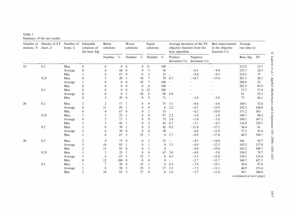
Table 1Summary of the test results

Number ofstations, N

Density of FTchart, d

Number ofloops, L

Infeasiblesolutions ofthe base Alg.

Bettersolutions

Worsesolutions

Equalsolutions

Average deviation of the TSobjective function from thebase algorithm

Best improvementin the objectivefunction (%)

Averagerun time (s)

Number % Number % Number % Positivedeviation (%)

Negativedeviation (%)

Base Alg. TS

10 0.2 Max. 0 0 0 0 0 11 100 – – – 212.9 15.7Average 0 4 44 0 0 5 56 – �6.1 �9.4 233.7 24.5Min. 1 4 67 0 0 2 33 – �0.4 �0.5 214.2 57

0.25 Max. 0 2 20 1 10 7 70 0.7 �14.7 �15.4 281.1 20.1Average 1 0 0 0 10 7 100 – – – 298.8 23Min. 0 0 0 0 0 6 100 – – – 282.3 65.9

0.5 Max. 0 0 0 0 0 12 100 – – – 75.7 17.4Average 0 0 0 2 20 8 80 6.8 – – 81 25.1Min. 0 2 29 0 0 5 71 – �2.8 �2.8 73 66.1

20 0.2 Max. 2 2 17 1 8 9 75 3.1 �0.6 �6.0 160.1 52.8Average 0 11 92 1 8 0 0 2.2 �6.7 �13.9 162.3 144.8Min. 0 4 67 0 0 2 33 – �6.3 �10.8 171.2 363

0.25 Max. 1 3 25 1 8 8 67 2.2 �1.0 �1.0 109.7 60.2Average 0 2 17 1 8 9 75 3.8 �1.0 �1.0 109.1 107.1Min. 1 5 45 1 9 5 45 6.7 �5.1 �6.5 116.9 239.1

0.5 Max. 1 6 50 1 8 5 42 0.2 �11.4 �17.1 36.4 61Average 2 6 50 0 0 6 50 – �6.6 �11.0 37.3 91.6Min. 1 8 67 3 25 1 8 5.7 �8.9 �17.4 40.5 198.7

30 0.2 Max. 2 9 75 0 0 2 25 – �4.5 �14.0 166 92.7Average 3 10 83 1 8 1 8 3.1 �4.9 �12.5 145.3 137.8Min. 2 11 92 0 0 1 8 – �8.0 �19.0 165.2 309.7

0.25 Max. 1 3 25 1 8 8 67 2.0 �4.8 �5.0 150.5 78.7Average 1 8 67 3 25 1 8 4.5 �5.3 �12.8 154.1 135.4Min. 0 12 100 0 0 0 0 – �2.7 �11.7 160.7 427.1

0.5 Max. 1 7 58 4 33 1 8 6.3 �7.9 �19.1 50.4 87.6Average 1 8 58 3 25 2 17 2.3 �7.5 �11.1 44.9 151.6Min. 2 10 83 2 17 0 0 1.8 �5.7 �11.8 50.1 244.6

(continued on next page)

G.

La

po

rteet

al.

/A

pp

liedM

ath

ema

ticsa

nd

Co

mp

uta

tion

18

3(

20

06

)1

41

0–

14

21

1417

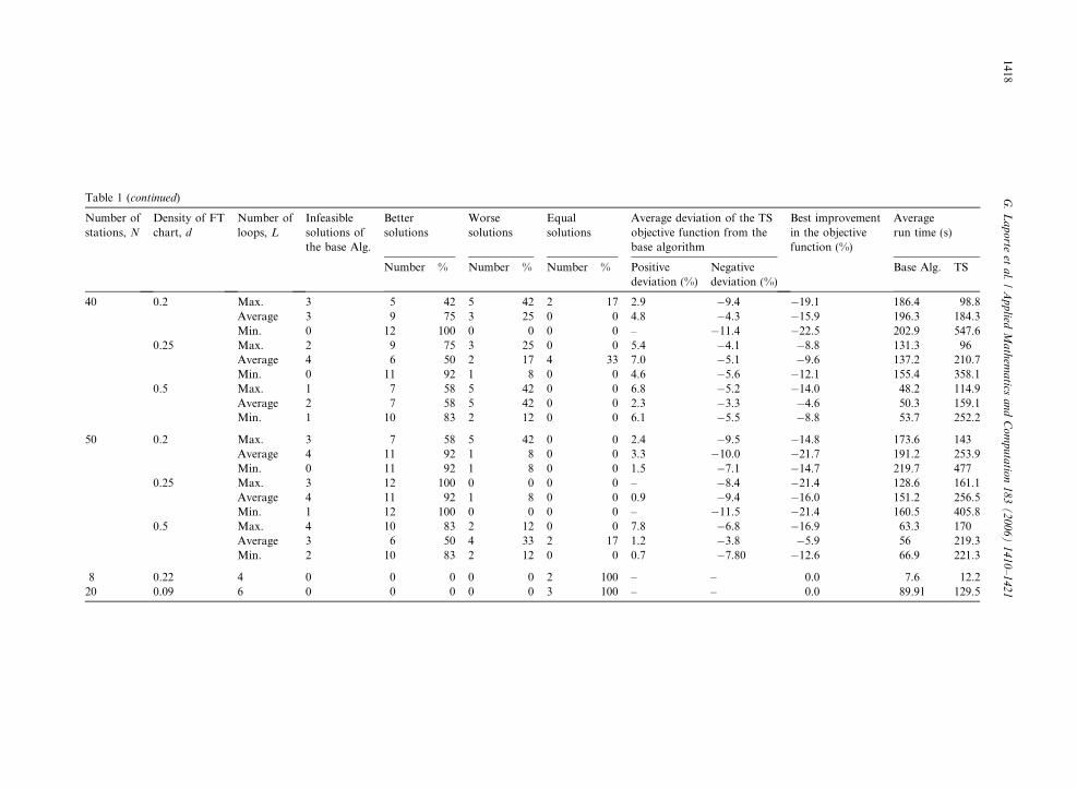
Table 1 (continued)

Number ofstations, N

Density of FTchart, d

Number ofloops, L

Infeasiblesolutions ofthe base Alg.

Bettersolutions

Worsesolutions

Equalsolutions

Average deviation of the TSobjective function from thebase algorithm

Best improvementin the objectivefunction (%)

Averagerun time (s)

Number % Number % Number % Positivedeviation (%)

Negativedeviation (%)

Base Alg. TS

40 0.2 Max. 3 5 42 5 42 2 17 2.9 �9.4 �19.1 186.4 98.8Average 3 9 75 3 25 0 0 4.8 �4.3 �15.9 196.3 184.3Min. 0 12 100 0 0 0 0 – �11.4 �22.5 202.9 547.6

0.25 Max. 2 9 75 3 25 0 0 5.4 �4.1 �8.8 131.3 96Average 4 6 50 2 17 4 33 7.0 �5.1 �9.6 137.2 210.7Min. 0 11 92 1 8 0 0 4.6 �5.6 �12.1 155.4 358.1

0.5 Max. 1 7 58 5 42 0 0 6.8 �5.2 �14.0 48.2 114.9Average 2 7 58 5 42 0 0 2.3 �3.3 �4.6 50.3 159.1Min. 1 10 83 2 12 0 0 6.1 �5.5 �8.8 53.7 252.2

50 0.2 Max. 3 7 58 5 42 0 0 2.4 �9.5 �14.8 173.6 143Average 4 11 92 1 8 0 0 3.3 �10.0 �21.7 191.2 253.9Min. 0 11 92 1 8 0 0 1.5 �7.1 �14.7 219.7 477

0.25 Max. 3 12 100 0 0 0 0 – �8.4 �21.4 128.6 161.1Average 4 11 92 1 8 0 0 0.9 �9.4 �16.0 151.2 256.5Min. 1 12 100 0 0 0 0 – �11.5 �21.4 160.5 405.8

0.5 Max. 4 10 83 2 12 0 0 7.8 �6.8 �16.9 63.3 170Average 3 6 50 4 33 2 17 1.2 �3.8 �5.9 56 219.3Min. 2 10 83 2 12 0 0 0.7 �7.80 �12.6 66.9 221.3

8 0.22 4 0 0 0 0 0 2 100 – – 0.0 7.6 12.220 0.09 6 0 0 0 0 0 3 100 – – 0.0 89.91 129.5

1418G

.L

ap

orte

eta

l./

Ap

plied

Ma

them

atics

an

dC

om

pu

tatio

n1

83

(2

00

6)

14

10

–1

42

1

G. Laporte et al. / Applied Mathematics and Computation 183 (2006) 1410–1421 1419

two or three stations for Lmax, and finally for Laverage was set to a value between the zH of Lmax and Lmin, orthe average workload for loops with sizes equal to [N/L]. Due to the assumption of at most one singleton sta-tion in the final configuration obtained from the TS algorithm, the same assumption was made for the basealgorithm as well.

The first two phases of the base algorithm which consist of generating subsets of stations and eliminatingsome of them were coded in Matlab 6.5 and the IP model was coded in LINGO 8.0 software ([29]) and finallythe TS algorithm was coded in Matlab 6.5. It was found that in most cases the effective size of the tabu list is[N/5] ± 2. Three randomly selected initial solutions were used for each problem, except for some small prob-lems where the number did not reach three.

4.3. Comparison of algorithms

Tests were carried out on a 2.00 GHz Intel Pentium 4, with 256 MB RAM. The summary of the test resultsis shown in Table 1. The last two rows in the table correspond to the two examples of Bozer and Srinivasan [9].The statistics of the Table 1 are summarized in Table 2. In small problems, the objective functions of the twoalgorithms are often equal to each other, which means optimal solutions. The percentage of better solutionssignificantly increases with the instance size N.

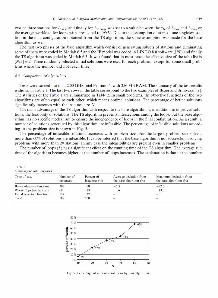
The main advantage of the TS algorithm with respect to the base algorithm is, in addition to improved solu-tions, the feasibility of solutions. The TS algorithm prevents intersections among the loops, but the base algo-rithm has no specific mechanism to ensure the independence of loops in the final configuration. As a result, anumber of solutions generated by this algorithm are infeasible. The percentage of infeasible solutions accord-ing to the problem size is shown in Fig. 5.

The percentage of infeasible solutions increases with problem size. For the largest problem size solved,more than 60% of solutions are infeasible. It can be inferred that the base algorithm is not successful in solvingproblems with more than 20 stations. In any case the infeasibilities are present even in smaller problems.

The number of loops (L) has a significant effect on the running time of the TS algorithm. The average runtime of the algorithm becomes higher as the number of loops increases. The explanation is that as the number

Table 2Summary of solution cases

Type of case Number ofinstances

Percent ofinstances (%)

Average deviation fromthe base algorithm (%)

Maximum deviation fromthe base algorithm (%)

Better objective function 303 60 �6.3 �22.5Worse objective function 68 13 3.6 13.3Equal objective function 137 27 – –Total 508 100 – –

6%

22%

36%

44%

67%

0%

10%

20%

30%

40%

50%

60%

70%

80%

10 20 30 40 50 60N

perc

ent

infe

asib

le

Fig. 5. Percentage of infeasible solutions by base algorithm.

1420 G. Laporte et al. / Applied Mathematics and Computation 183 (2006) 1410–1421

of stations in the loops increases, more time is required to compute the workloads. In comparison with thebase algorithm, the TS algorithm is often faster for lower flow densities and higher L values. In general itseems that on larger problems the base algorithm tends to be faster than TS, but the latter algorithm remainspreferable because it always produces feasible solutions.

5. Conclusions

We have proposed a new TS algorithm for designing of AGV routes in a tandem configuration. Our heu-ristic was compared to the base heuristic of Bozer and Srinivasan [9]. The two algorithms were run on 60 ran-domly generated problems at three levels of loop numbers. TS algorithm was applied to two instancesdescribed by Bozer and Srinivasan [9]. Results show that our algorithm is capable of producing better solu-tions and the amount of improvements in the objective function with respect to the base algorithm tends tobe higher as the problem size increases. The main advantage of our TS algorithm is the impossibility of gen-erating overlapping loops. Results show that as the problem size increases, the likelihood of generating infea-sible solutions is very high for the base algorithm.

Acknowledgements

This work was partially supported by the Canadian Natural Sciences and Engineering Research Councilunder Grant OGP00039682. We thank Farhang Fasihi for his valuable comments.

References

[1] A. Aarab, H. Chetto, L. Radouance, Flow Path Design for AGV Systems (2001). Available from: <http://www.ici.ro/ici/revista/sic99_2/art02.html>.

[2] A. Asef-Vaziri, G. Laporte, Loop based facility planning and material handling, Eur. J. Operat. Res. 164 (2005) 1–11.[3] A. Asef-Vaziri, M. Dessouky, C. Sriskandarajah, A loop material flow system design for automated guided vehicles, Int. J. Flex.

Manuf. Sys. 13 (2001) 33–48.[4] A. Asef-Vaziri, G. Laporte, C. Sriskandarajah, The block layout shortest loop design problem, IIE Trans. 32 (2000) 724–734.[5] P. Banerjee, Y. Zhou, Facilities layout design optimization with single loop material flow path configuration, Int. J. Prod. Res. 33

(1995) 183–203.[6] M. Barad, D. Sinriech, A Petri net model for the operational design and analysis of segmented flow topology (SFT) AGV system, Int.

J. Prod. Res. 36 (1998) 1401–1426.[7] Y.A. Bozer, M.M. Srinivasan, Tandem configurations for AGV systems offer simplicity and flexibility, Ind. Eng. 21 (1989) 23–27.[8] Y.A. Bozer, M.M. Srinivasan, Tandem configuration for automated guided vehicle systems and the analysis of single vehicle loops,

IIE Trans. 23 (1991) 72–82.[9] Y.A. Bozer, M.M. Srinivasan, Tandem AGV systems: a partitioning algorithm and performance comparison with conventional AGV

systems, Eur. J. Operat. Res. 63 (1992) 173–191.[10] Y.A. Bozer, C.G. Lee, Using existing workstations as transfer stations in tandem AGV systems, J. Manuf. Sys. 23 (2004) 229–241.[11] D. Chhajed, B. Montreuil, T. Lowe, Flow network design for manufacturing systems layout, Eur. J. Operat. Res. 57 (1992) 145–161.[12] R.Z. Farahani, G. Laporte, Two Formulations for Designing Optimal Single Loop and the Location of P/D Stations, IIEC 2004

Conference, Tehran, Iran, July 13–14, 2004.[13] R.Z. Farahani, G. Laporte, M. Sharifyazdi, A practical exact algorithm for the shortest loop design problem in a block layout, Int. J.

Prod. Res. 43 (2005) 1879–1887.[14] R.Z. Farahani, F.G. Tari, A branch and bound method for finding flow-path designing of AGV systems, IIE Trans. A: Basics 15

(2002) 81–90.[15] R.Z. Farahani, F.G. Tari, Optimal flow path designing of unidirectional AGV systems, Int. J. Eng. Sci. 12 (2001) 31–44.[16] B.E. Farling, C.T. Mosier, F. Mahmoodi, Analysis of automated guided vehicle configuration in flexible manufacturing systems, Int.

J. Prod. Res. 39 (2001) 4239–4260.[17] R.J. Gaskin, J.M.A. Tanchoco, Flow path design for automated guided vehicle system, Int. J. Prod. Res. 25 (1987) 667–676.[18] R.J. Gaskin, J.M.A. Tanchoco, F. Taghaboni, Virtual flow paths for free ranging automated guided vehicle systems, Int. J. Prod. Res.

27 (1989) 91–100.[19] L.F. Hsieh, D.Y. Sha, A design process for tandem automated guided vehicle systems: the concurrent design of machine layout and

guided vehicle routes in tandem automated guided vehicle systems, Integ. Manuf. Sys. 7 (1996) 30–38.[20] C. Huang, Design of material transportation system for tandem automated guided vehicle systems, Int. J. Prod. Res. 35 (1997)

943–953.[21] M. Kaspi, U. Kesselman, J.M.A. Tanchoco, Optimal solution for the flow path design problem of a balanced unidirectional AGV

system, Int. J. Prod. Res. 40 (2002) 349–401.

G. Laporte et al. / Applied Mathematics and Computation 183 (2006) 1410–1421 1421

[22] M. Kaspi, J.M.A. Tanchoco, Optimal flow path design of unidirectional AGV systems, Int. J. Prod. Res. 28 (1990) 1023–1030.[23] C.W. Kim, J.M.A. Tanchoco, Conflict-free shortest-time bi-directional AGV routing, Int. J. Prod. Res. 29 (1991) 2377–2391.[24] K.C. Ko, P.J. Egbelu, Unidirectional AGV guide path network design: a heuristic algorithm, Int. J. Prod. Res. 41 (2003) 2325–2343.[25] P. Kouvelis, G.J. Gutierrez, W.C. Chiang, Heuristic unidirectional flow path design approach for automated guided vehicle systems,

Int. J. Prod. Res. 30 (1992) 1327–1351.[26] G. Laporte, A. Asef-Vaziri, C. Sriskandarajah, Some application of the generalized traveling salesman problem, J. Oper. Res. Soc. 47

(1996) 1461–1467.[27] J.T. Lin, C.C.K. Chang, W.C. Liu, A load routing problem in a tandem-configuration automated guided vehicle system, Int. J. Prod.

Res. 32 (1994) 411–427.[28] S. Rajagopalan, S.S. Heragu, G.D. Taylor, A Lagrangian relaxation approach to solving the integrated pick-up/drop-off point and

AGV flow path design problem, Appl. Math. Model. 28 (2004) 735–750.[29] A. Roe, User’s Guide for LINDO and LINGO, Windows Versions, Duxbury Press, Belmont, CA, 1997.[30] E.A. Ross, F. Mahmoodi, C.T. Mosier, Tandem configuration automated guided vehicle systems: a comparative study, Decision Sci.

27 (1996) 81–102.[31] G.A.F. Seber, Multivariate Observations, Wiley, New York, 1984.[32] Y. Seo, P.J. Egbelu, Flexible guide path design for automated guided vehicle systems, Int. J. Prod. Res. 33 (1995) 1135–1156.[33] D. Sinriech, J.M.A. Tanchoco, Intersection graph method for AGV flow path design, Int. J. Prod. Res. 29 (1991) 1725–1732.[34] D. Sinriech, J.M.A. Tanchoco, Solution methods for the mathematical models of single loop AGV systems, Int. J. Prod. Res. 31

(1993) 705–726.[35] D. Sinriech, J.M.A. Tanchoco, SFT – segmented flow topology, in: J.M.A. Tanchoco (Ed.), Material Flow System in Manufacturing,

Chapter 8, Chapman and Hall, London, 1994, pp. 200–235.[36] D. Sinriech, J.M.A. Tanchoco, An introduction to the segmented flow approach to discrete material flow systems, Int. J. Prod. Res. 33

(1995) 3381–3410.[37] D. Sinriech, J.M.A. Tanchoco, Design procedures and implementation of the segmented flow topology (SFT) for discrete material

flow systems, IIE Trans. 29 (1997) 323–335.[38] X.-C. Sun, N. Tchernev, Impact of empty vehicle flow on optimal flow path design for unidirectional AGV systems, Int. J. Prod. Res.

34 (1996) 2827–2852.[39] J.M.A. Tanchoco, D. Sinriech, OSL – optimal single loop guide paths for AGVs, Int. J. Prod. Res. 30 (1992) 665–681.[40] J.A. Tompkins, J.A. White, Y.A. Bozer, J.M.A. Tanchoco, Facilities Planning, third ed., Wiley, Chichester, 2003.[41] M.A. Venkataramanan, K.A. Wilson, A branch- and bound algorithm for flow path design of automated guided vehicle systems,

Nav. Res. Logist. Q. 38 (1991) 431–445.[42] J.A. Ventura, C. Lee, Tandem loop with multiple vehicles configuration for automated guided vehicle systems. Available from:

<fie.engrng.pitt.edu/iie2002/proceedings/ierc/papers/2222.pdf> (2001).[43] W. Yu, P. Egbelu, Design of a variable path tandem layout for automated guided vehicle systems, J. Manuf. Sys. 20 (2001) 305–319.