design and implementation of an inshore hydrographic ... · design and implementation of an inshore...
TRANSCRIPT

DESIGN AND IMPLEMENTATION OF AN
INSHORE HYDROGRAPHIC SURVEYING SYSTEM
P. E. HOURDAKIS
January 1986
TECHNICAL REPORT NO. 120

PREFACE
In order to make our extensive series of technical reports more readily available, we have scanned the old master copies and produced electronic versions in Portable Document Format. The quality of the images varies depending on the quality of the originals. The images have not been converted to searchable text.

DESIGN AND IMPLEMENTATION OF AN INSHORE HYDROGRAPHIC SURVEYING
SYSTEM
Pantelis Emmanuil Hourdakis
This report is an unaltered printing of the author's Master of Science in Engineering thesis
submitted to this department in December 1985
Department of Surveying Engineering University of New Brunswick
P.O. Box 4400 Fredericton, N.B.
Canada E3B5A3
January 1986
Latest Reprinting September 1992

ABSTRACT
Computers are now widely used in hydri)Jraphic surveys to tal<e advent~ of their ab111ty
to provide navigation function and data processing capabilities. The design parameters that play aQ
important role when we try to create an automatic data acquisition and processing system are the
accuracy with which sea bottom is represented, the reliability, the compatibility with existing
hardware, the man/machine interaction, the modularity and the cost of the system.
In order to optimize the design parameters, an automatic data acquisition and processing
system was built around the Apple lie personal computer. The algorithms required to meet the
design objectives have been implemented in larger systems. These systems are down scaled to a
system that will serve the needs of near shore hydrography. Different systems of lines, used to
sample the depth, are compared: straight parallel lines, lines of position of electronic positioning
systems, circles and radial lines ("star" mode). In order to filter the position data simple gating
techniques are compared with Least Squares and Kalman Filters. In order to filter the depth data
depth filtering techniques are examined.
The results indicate that the Apple lie with commercially available peripherals and
standard software, offers great promise of replacing larger and more expensive hydri)Jraphic data
acquisition and navigation controllers. Straight parallel lines give efficient cover~ of the survey
area only if they can be modified on-line. The "star" mode is the best shoal examination pattern
with respect to track keeping ab111ty. The memory and computational speed constraints of
personal computers require the use of simple linear filters to filter the position data. Visual
comparison of digital depths with anaii)J depths is an efficient depth filtering technique.
- ii -

TABLE OF CONTENTS
Page
ABSTRACT ............................................................. ii
TABLE OF CONTENTS.................................................... iii
LIST Of fiGURES. . . . . . . . . . . . . . . . . . . . . . . . . . . . . . . . . . . . . . . . . . . . . . . . . . . . . . . v
LIST OF TABLES.. . . . . . . . . . . . . . . . . . . . . . . . . . . . . . . . . . . . . . . . . . . . . . . . . . . . . . . vii
ACKNOWLEDGEMENTS. . . . . . . . . . . . . . . . . . . . . . . . . . . . . . . . . . . . . . . . . . . . . . . . . . . viii
I. INTRODUCTION ..................................................... .
1. I Elements of a Hydrograpfic Survey System. . . . . . . . . . . . . . . . . . . . . . . . . . . . 2
1.2 Automated survey systems. . . . . . . . . . . . . . . . . . . . . . . . . . . . . . . . . . . . . . . . . . 3
1.3 Main contribution of this thesis. . . . . . . . . . . . . . . . . . . . . . . . . . . . . . . . . . . . . 5
1. 4 Outline of the thesis. . .. .. .. .. .. .. . . . . . .. . .. .. . . . . . . .. .. . . .. .. .. . . . 7
2. DESIGN CRITERIA and REVIEW OF EXISTING SYSTEMS. . . . . . . . . . . . . . . . . . . . . . . . 9
2. I Accurac.y of sea bottom representation . . . . . . . . . . . . . . . . . . . . . . . . . . . . . . . . 9
2.2 Reliability . . . . . . . . . . . . . . . . . . . . . . . . . . . . . . . . . . . . . . . . . . . . . . . . . . . . . . 13
2.3 Man/machine interaction. . . . . . . . . . . . . . . . . . . . . . . . . . . . . . . . . . . . . . . . . . . 14
2. 4 Mooularity and portability. . . . . . . . . . . . . . . . . . . . . . . . . . . . . . . . . . . . . . . . 18
2.5 Compatibility. . . . . . . . . . . . . . . . . . . . . . . . . . . . . . . . . . . . . . . . . . . . . . . . . . . 20
2.6Cost ........................................................... 21
2. 7 Review of existing systems. . . . . . . . . . . . . . . . . . . . . . . . . . . . . . . . . . . . . . . . . 22
3. DATA ACQUISITION and ON-LINE DATA PROCESSING. . . . . . . . . . . . . . . . . . . . . . . . . 27
3.1 General system configuration.. . . . . . . . . . . . . . . . . . . . . . . . . . . . . . . . . . . . . . 27
3. 1. 1 Position input. . . . . . . . . . . . . . . . . . . . . . . . . . . . . . . . . . . . . . . . . . . . . 29
3. 1.2 Depth input. .. .. . .. . . .. . .. . .. .. . . .. .. . .. .. . .. . . . .. . .. . . . .. 30
3. 1.3 Central Processing Unit. . . . .. .. .. . .. . . . . . .. . . . .. . .. .. . .. . .. . 30
- iii -

Pege
3. 1. 4 Acquisition software . . . . . . . . . . . . . . . . . . . . . . . . . . . . . . . . . . . . . . . . 31
3.2 The INTERFACE mooule. . . . . . . . . . . . . . . . . . . . . . . . . . . . . . . . . . . . . . . . . . . . 34
3.3 The QUALITY CONTROL module ....................................... 40
3.3. 1 Nature of positioning errors. . . . . . . . . . . . . . . . . . . . . . . . . . . . . . . . . . . 40
3.3.2 Nature of bathymetric errors. . . . . . . . . . . . . . . . . . . . . . . . . . . . . . . . . . 43
3.3.3 Quality control of positioning data. . . . . . . . . . . . . . . . . . . . . . . . . . . . . . . 45
3.3.4 Quality control of bathymetric data. . . . . . . . . . . . . . . . . . . . . . . . . . . . . 52
3.4 The NAVIGATION mooule ............................................ 53
3.4. 1 Primary survey lines. . . . . . . . . . . . . . . . . . . . . . . . . . . . . . . . . . . . . . . . 57
3.4.2 Investigation of seabed features. . . . . . . . . . . . . . . . . . . . . . . . . . . . . . . . . 60
3.4.3 Cross and junction lfnes. . . . . . . . . . . . . . . . . . . . . . . . . . . . . . . . . . . . . . 63
3.5 The ON-LINE MODIFICATION mooule. . . . . . . . . . . . . . . . . . . . . . . . . . . . . . . . . . 65
3.6 Description of current version of data acquisition system (SEAHATS). . . . . . . 6 7
4. Off-LINE DATA PROCESSINO.......................................... 70
4.1 Oeneral processing considerations. . . . . . . . . . . . . . . . . . . . . . . . . . . . . . . . . . . 70
4.2 lnterew::tive editing of hydrographic data. . . . . . . . . . . . . . . . . . . . . . . .. . . . . . . 72
4.3 Smoothing, correction and reduction of hydrographic data . . . . . . . . . . . . . . . . 73
4.3. 1 Smoothing of positioning data. . . . . . . . . . . . . . . . . . . . . . . . . . . . . . . . . . 75
4.3.2 Correction of speed of sound in water. . . . . . . .. . . . . . . . . . . . . . . . . .. . 79
4.3.3 Datum reduction. . . . . . . . . . . . . . . . . . . . . . . . . . . . . . . . . . . . . . . . . . . 81
4.3.4 Establfshment of the sounding datum. . . . . . . . . . . . . . . . . . . . . . . . . . . . 84
4.3.5 Roll, pitch, heave corrections................................. 86
4. 4 Selection and preSentation of results. . . . . . . . . . . . . . . . . . . . . . . . . . . . .. . . . . 91
4. 4. 1 Selection of soundings. . . . . . . . . . . . . . . . . . . . . . . . . . . . . . . . . . . . . . . . 91
4. 4.2 Shoal detection. . . . . . . . . . . . . . . . . . . . . . . . . . . . . . . . . . . . . . . . . . . . . . 92
4. 4.3 Presentation of results. . . . . . . . . . . . . . . . . . . . . . . . . . . . . . . . . . . . . . . 94
- iv -

Page
4.4."1 Data base management....................................... 96
"1.5 Description of SEAHATS d6ta processing pac!(age. . . . . . . . . . . . . . . . . . . . .. . . . . 97
5. TESTS and RESULTS. . . . . . . . . . . . . . . . . . . . . . . . . . . . . . . . . . . . . . . . . . . . . . . . . . 101
5. 1 Tests description and objectives. . . . . . . . . . . . . . . . . . . . . . . . . . . . . . . . . . . . . . 1 01
5.2 Accuracy. . . . . . . . . . . . . . . . . . . . . . . . . . . . . . . . . . . . . . . . . . . . . . . . . . . . . . . 1 04
5.3 Man/machine interaction. . . . . . . . . . . . . . . . . . . . . . . . . . . . . . . . . . . . . . . . . . 111
5. 4 SEAHA TS software evaluation. . . . . . . . . . . . . . . . . . . . . . . . . . . . . . . . . . . . . . . 113
6. CONCLUSIONS and RECOMMENDATIONS. . . . . . . . . . . . . . . . . . . . . . . . . . . . . . . . . . . 120
L 1ST OF REFERENCES. . . . . . . . . . . . . . . . . . . . . . . . . . . . . . . . . . . . . . . . . . . . . . . . . . 124
APPENDIX I : Navigation a1!1)rithms for track following. . . . . . . . . . . . . . . . . . .. . . . . 130
LIST OF FIOURES
Page
Figure 1. 1 : Basic relationship among the survey elements at the level of the Survey
System related to oota acquisition.. . . . . . . . . . . . . . . . . . . . . . . . . . . . . . . 4
2.1 :Types of LIR indicators. . . . . . . . . . . . . . . . . . . . . . . . . . . . . . . . . . . . . . . . . 17
2.2 : The development process. . . . . . . . . . . . . . . . . . . . . . . . . . . . . . . . . . . . . . . . 19
3. 1 : Block diagram of a navigation and hydrographic d6ta acquisltion controller 28
3.2: Information flow among the elements of an ideal navigation and
hydrographic d6ta acquisition controller. . . . . . . . . . . . . . . . . . . . . . . . . . 32
3.3: A program Controlled Input/ Output. . . . . . . . . . . . . . . . . . . . . . . . . . . . . . 36
3.4: An interrupt Controlled Input/ Output............................ 36
- v -

Page
Figure 3.5: An "intelligent" interface.. . . . . . . . . . . . . . . . . . . . . . . . . . . . . . . . . . . . . 38
3.6 : The forms of transmitted and received pulses in Mini Ranger. . . . . . . . . 42
3.7: Ranoom errors in Mini Ranger.................................. 42
3.8: A typical echogram............................................ 42
3. 9 : Distortion of seabed due to beamwidth. . . . . . . . . . . . . . . . . . . . . . . . . . . . . 44
3.10: Gating techniques to detect range spik.es. . . . . . . . . . . . . . . . . . . . . . . . . . 48
3. 11 : The fixed memory range filter. . . . . . . . . . . . . . . . . . . . . . . . . . . . . . . . . . 48
3. 12 : Statistical efficienLY and dynamic response of range filters
(from Casey, 1982) ......................................... 50
3.13: The sea bottom tracking gate... . . . . . . . . . . . . . . . . . . . . . . . . . . . . . . . . 54
3.14: The sequence of task.s needed to apply a scale factor.. . . . . . . . . . . . . . . . 54
3.15: The sounding system of parallel straight lines. . . . . . . . . . . . . . . . . . . . 58
3. 16 : Shoal exam1nat1on patterns. . . . . . . . . . . . . . . . . . . . . . . . . . . . . . . . . . . 62
3. 17 : Types of junction lines .................................. ;<. • • • 64
3. 18 : Wft./ point navigation. . . . . . . . . . . . . . . . . . . . . . . . . . . . . . . . . . . . . . . . . 64
3.19 : Flow chart of the NAVIGATION module. . . . . . . . . . . . . . . . . . . . . . . . . . . . 66
4.1 :Corrections and reductions to observed soundings.. . . . . . . . . . . . . . . . . . . 74
4.2: Estimation of Mini Ranger range rate time series with Kalman filtering
for various gain factors. . . . . . . . . . . . . . . . . . . . . . . . . . . . . . . . . . . . . . . . 78
4.3 : Sound velocity profile in the area of survey. . . . . . . . . . . . . . . . . . . . . . . . 82
4. 4 : Seasonal variation of water level in Saint John river. . . . . . . . . . . . . . . . . 82
4.5 : Semi-diurnal tide at campobello Island and its sine curve approximation. 85
4.6 : Ship motion due to wave action and its effect on depth ootermination and
position of the antenna of positioning system.. . . . . . . . . . . . . . . . . . . . . . . 88
4. 7 : Depth error due the roll and pitch of the vessel over a flat , horizontal,
1 00 metres deep seabed. . . . . . . . . . . . . . . . . . . . . . . . . . . . . . . . . . . . . . . 89
- vi -

Page
Figure 4.8 : Geometric probability of finding an underwater obstacle. . . . . . . . . . . . . 93
4.9: The processing phases.. . . . . . . . . . . . . . . . . . . . . . . . . . . . . . . . . . . . . . . . 100
5. 1 : The test site (from CHS chart 4373) . . . . . . . . . . . . . . . . . . . . . . . . . . . . . 1 03
5.2: Time series of range from channel B of Mini Ranger.. . . . . . . . . . . . . . . . 105
5.3 : Analog and digital depths over an irregular seabed. . . . . . . . . . . . . . . . . . . 1 06
5. 4 : Analog and digital depths over a relatively flat seabed . . . . . . . . . . . . . . . . 1 07
5.5 : Computation time versus cycle number for various sampling intervals. . 110
5.6 : Ship's tracks while running parallel straight lines . . . . . . . . . . . . . . . . . 1 t 2
5. 7 : Ship's tracks while doing shoal examination ( mooified "star" mroe). . . . 114
5.8 : Ship's tracks while doing shoal examination ("circles" mroe) . . . . . . . . . t 15
5. 9 : Ship's tracks while doing shoal examination ( "star" mOOe) . . . . . . . . . . . 116
5. t 0 : Final field sheet . . . . . . . . . . . . . . . . . . . . . . . . . . . . . . . . . . . . . . . . . . . . . 119
I . t : The geometry of parallel straight lines and Wflo/ point navigation . . . . . . . 133
I .2 : The geometry of "star" mroe shoal examination . . . . . . . . . . . . . . . . . . . . . 134
I .3 : The geometry of "circles" mroe shoal examination . . . . . . . . . . . . . . . . . . . 135
LIST OF TABLES
Page
Table 3. 1 : Error sources and error magnitudes in depth determination
(from Eaton 1968) . . . . . . . . . . . . . . . . . . . . . . . . . . . . . . . . . . . . . . . . . . . 44
4. 1 : tv:;curfD/ ( RMS errors) of determination of water level using a
3-dflol perioo of observations (from Aboh 1983) . . . . . . . . . . . . . . . . . . . 85
5.1 :Size order of the average of off-track error in a sample of 7 survey legs.. t 10
5.2: Hard copy of collected soundings... . . . . . . . . . . . . . . . . . . . . . . . . . . . . . . . 118
- vii -

ACKNOWLEDOEMENTS
I wish to express my deep gratitude and appreciation to my supervisor Dr. David E. Wells
for his interest, support and guidance. Always available when difficulties arose, his expert
suggestions and encouragement were invaluable. In frljition, while exploring the aspects of
hydrography, I found his lectures to be of immense help.
I would also li"e to express my appreciation to the members of the Examining Board, Dr.
A. Chrzanowski of the Deparment of Surveying Engineering and Dr. J. Tranquilla of the
Department of Electrical Engineering, for their thoughtful comments.
The flnancial support provided by the National Sciences and Engineering Research Council
of canada operating grant "Arctic Navigation/Satellite Positioning" and strategic grants "Marine
GeOOecy" and "Applications of Marine Geodesy", all held by Dr. D. E. Wells, is gratefully
acknowledged. Financial support was also provided by the University of New Brunswick.
Many people provided assistance at various stages of my research. I am deeply indebted to
Dr. Richard B. Langley and to Mr. See Hean Quek for their critical comments and helpful
discussions about this thesis. I am also indebted to the Bedford lnstitude of Oceanography and the
canadian Hydrographic Service for the equipment they provided and for sharing their many years
of exper1ence 1n hydrograph1c operat1ons.
For proof-reading the entire thesis, I would like to deeply thank Mrs. Anne Armenalds,
Mr. Owen West and Mr. See Hean Quelc
I also thank my graduate colleagues for their continuous encouragement, support and
friendship. Particularly, Anton is and Costas Armenakis, Marinos Kavouras, Stelios Mertikas and
- viii -

Stratis Tsamouras were of great help during the difficult moments of my groouate studies. To my
wife Maria, for her encouragement, understanding and moral support, a heartfelt thanlc you is not
enough. Her w1111ngs to see my worlc to its completion made my studies much more easier.
Finally, I express my gratitude to professor George Veis of the National Technical
University of Athens who introduced me to the art of hydrography.
- ix -

1. INTRODUCTION
The purpose of this thesis is to define the design parameters for an automated data
acquisition and processing system and to desribe the development and testing of a specific system
that optimizes these parameters for inshore hydrographic survey : a detailed description of the
sea bottom including measurements of tides and currents in depths of 40 metres or less
(Umbach, 1916 ). The end product of such a system is a chart or a set of bottom profiles at
scales 1:20000 or larger, unless smaller scales are specified in the project instructions.
Activities that require the use of such a system are :
- charting of navigational waters,
- dredging operations for development and conservancy of harbours and waterways,
- examinations of areas to confirm or contradict the existence of seabed obstructions
indicated by previous surveys and
- searches for reported seabed features l Ingham, 1914 ) .
This chapter incorporates the data acquisition and processing system with the
Hydrographic Survey System, summarizes the contribution of the thesis and gives an outline of the
subsequent chapters.
- 1 -

1.1 Elements of e Hydrographic Survav System
As specified In the pro;ress report for Data Acquisition and Processing Systems ( F/8 ,
1911 ) , a Hydrographic survey System consists of six major Inter-related elements: survey
planning, data !P!Uisltion, data processing,~ mangment, support_ functtc:m~ and survey
environment.
Survey olannina is the selection of the steps that will lEHI to an efficient achievement of
the client's requirements. For example, if the requirement is ·safe p8SS8Qe of ships of some
maximum draW, survey planning will delineate the area to be surveyed end the accuraL)' with
which the bottom must be represented. These requirements are translated into the necessary
equipment, time, personnel, cost and methcrlllogy of the survey. Details on survey planning can be
found in Ingham ( 1914) and, Surveys and /1applng Branch ( 1982).
Data ocgufsftfon Is the recording of Information from different sources using calibrated
Instruments at pre-defined IJ:CUrfK:Y standards. The survey vessel Is navigated along designated
tracks, the depth of water is sensed, and tidal heights are measured along with any other
Information that wm assist In representation of sea bottom topography.
Once the data has been acquired, data processing converts and presents it in a manner
most appropriate to the client's needs. This includes editing and correction of data, merging data
from different sources, selection of representative data and presentation of the data sample in a
comprehensive and efB./ to use format.
Survey manaooment has the responsibility of ensuring that the objectives of the survey
project have been met, while optimizing the available resources ( personnel, bud;Jet, equipment,
time etc.).
- 2 -

Survev suooort consists of various functions including the maintenance and use of
hydrographic boats, hiring and housing personnel, and the purchase and/or development of
equipment, to name a few.
The survey environment includes sea state, r~io and acoustic propagation problems as
well as the political and economic environment where the hydrographic survey takes place.
Figure 1. 1 lllustrates the basic relationship among the survey elements at the level of the
Survey System related to data~K:Quisition. For each day of survey work, survey planning specifies
the instruments, personnel and methodoiD;tf that wlll be used. The launch hydrographer ~K:QUires
soundings which after being processed, are analyzed by the survey manager (hydrographer-in
charge) who then updates the requirements for the work next day. These tasks are directly
influenced by the environment and survey support functions.
1.2 Automated survey systems
This thesis deals with the data m.~isition and data orocessina elements of a hydrographic
survey system. Comments are also included where these elements interact with the other elements
of the survey system. Both procedures (acquisition and processing) can be manual, automatic,
or semi-automatic. Manual methods such as horizontal sextant angle resection, subtense ranging
by single vertical angle, intersection from shore stations by theodolites, manual recording of
LOPs (lines Of Position) from r~io positioning systems still exist. Semi-automatic methods
provide the interm~iate steps necessary to complete automation. Automation implies the
development of computer assisted techniques for data gathering and processing. Data is converted
to digital form to be processed by the computer, which initially was 00ne off-line (e.g. use of
digitizing table to convert analog echosounder outputs to digital form). However, many survey
instruments are now desigged to provide an output that is directly compatible with digital data
~K:QUisition systems.
- 3 -
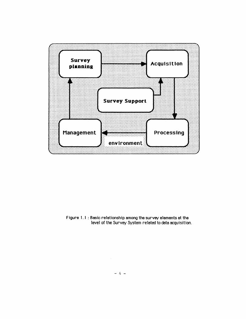
Figure I. I : Basic relationship among the survey elements at the level of the Survey System related to data fDlUisition.
- 4 -

Various authors have 1111ressed the gains which may be achieved by automation In
hydr~rephic surveys (11ackay, 1972,· 11acdonald et a!., 1975,· Janes, 198"1).
Computers provide automated error detection techniques and fast automated data tK:QUisltlon and
processing. This results In more fK:CUrate and comp Jete field data and In surveys which ere more
efficient In t1me, personnel and resources.
A review of the existirig-deta acqUisition systems shows that there are two approaches in
the design of en automatic data acquisition system. One approach is to use existing hardware
(specific microprocessor, 1/0 hardware) end build a system that is designated to oo a specific
number of teslcs. The other approach is to use "off-the-sheW computers with a standard
operating system allowing the use of "off-the-sheW compilers.
Many parameters play en important role when one tries to create a data ~~:Q~Jisition and
processing system according to one approach or the other. The distribution of data processing
functions between on-line ( on board ship ) and off-line ( on shore ), the amount and qualtty of
gathered data, and the man/machine Interaction ere some vital parameters that have to be taken
Into consideration when designing a system. Various organizations and companies have proposed
implementations geared towerds the optimum solution of design problems. A widespreo::l
phtlosophy Is to design systems which are hardware oriented, fast and store great amounts of data.
However, these systems are infiexible and incomoatible with a variety of peripherals. For
example, only straight lines are to be navigated (one line at a time) or the systems may not
provide navtgattonal cepab111ttes at all. Special hardware ts required to process the data.
1.3 Main contribution of this thesis
The research desribed in this thesis resulted in the development of a complete, working,
see-tested hydrographic data EK:QUisition and processing system, together with a complete user's
guide. This system has been given the name SEAHATS (Surveying Engineering Automatic
- 5 -

Hydrographic data Acquisition and Track control System). The philosophy Inherent to the oostgn
is that the 5y5tem will be:
a) software oriented,
b) easily modified to meet different requirements,
c) comosttble wtth extsttng hardware,
d) flexible for the user (e.g. different modes of operation) and
e) of low cost.
The backbone of the software structure for SEAHATS was created by 11c earthy
( 1983), however this first version of SEAHATS was lacking in flexibility and efficiency,
had not been sea-tested, had no post-processing capabilities and lacked many of the features of the
present 5y5tem.
The following topics were Investigated In order to meet the SEAHATS ooslgn obJectives :
1. An automatic hydrographic data ~uisition 5y5tem consists of a central computer, the
environmental sensors and peripherals as well as the hydrographer and the coxswain. Information
is exchanged among these elements. The speed and the manner (format, digital or analog) of
information exchanged is discussed in sections 3.1 and 3.2.
2. The survey vessel is navigated along lines of pre-defined geometric patterns. These
patterns may be parallel straight lines, circles etc .. The application, size and configuration of area
to be surveyed, sea bottom morphology, and the coxswain's experience fn hydrographic surveys
are some of the factors that govern the choice of a survey pattern. An evaluation of these patterns
is made and the most appropriate techniques have been implemented in SEAHATS. These are
discussed In section 3.4.
3. Data (positioning and bathymetric) must be filtered in order to be reliable. Many
filtering techniques exist (gating, Least Squares, Kalman filtering etc.). These techniques are
evaluated for use in inshore hydrographic surveys in section 3.3.
- 6 -

1.4 Outline of the thesis
This thesis Is divided Into six chapters. The sequence of chapters conforms to the sequence
of tasks Involved In hydrographic surveys : d8ta acquisition, on-line and off -line d8ta processing.
The acquisition and processing ai!Jrlthms are reviewed and developed or modified to fK:COmmod8te
the needs of Inshore hydrOJraphy. A brief description of them is as follows.
In chapter 2, the design criteria for a hydrographic data acquisition and processing system
are established with emphasis on the accuracy of the output and the flexibility of the system.
Detailed description can be found elsewhere (Boudreau I 19841• 1011 report 1 2 1 1982).
The current status of commercially available systems is reviewed and these systems are evaluated
with respect to the established criteria.
For the development of the navigation and hydrographic data acquisition controller, a
top-down design concept is adopted. In chapter 3, the system Is broken Into separate modules
Including : the tnterfo, quality control of observations, navigation, on-line modlflcatlon and
output modules. This chapter is devoted to the description of the direction and rate of information
flow between different modules, as well as to the description of eEdl module itself. The interfo
module describes the communication between the CPU (Central Processing Unit), operator,
positioning system and echosounder. The QUBlity control module investigates the errors Inherent
In positioning and bathymetric d8ta, end provides the means to eliminate them. The navigation
part deals with the algorithms used to steer the vessel and the systems of lines used to sample the
depth. Finally, SEAHATS Is described.
Chapter 4 deals with the off-line data processing procedures to edit, correct, reduce and
present the collected data. These procedures are not new and are widely used in the hydrographic
community. What has been absent (at least _in the systems used by Canadian Hydrographic
- 7 -

Service), is the ab1Hty to use them tn real time or almost real time to help the ·data collector·
in jUOJing the results. This chapter describes such a processing p8Ckage.
Chapter 5 is devoted to a brief description of the tests during the development history of
the system and the evaluation and explanation of the obtained results.
Chapter 6 gives the conclusions and recommend8tions for future work and development.
Appendix I contains the al~ithmsused to provide steering information to the coxswain to
keep the vessel on pre-determined traclcs. In order to facilitate the use of the system, a User's
Guide is available as the Technical Memorandum: Operating Manual and Software listings
for SEAHATS (Hourdakis, 1985). The difficulties encountered in testing the I'I:QUisition
software in reel time, gave rise to a simulation package ( Hourdak is, 1985), designed to
simulate, as realistically as possible, the marine sensor data supplied to the vessel at see.
- 8 -

2. DESIGN CRITERIA and REVIEW OF EXISTING SYSTEMS
The study of the requirements of an application, the philosophy behind the existing
~~:quisition and processing systems, and the experience gained in hydri)J'aphic operations reveals
a set of 005ign criteria that has to be satisfied. These are: ~rtLY of sea bottom representation,
reliability, man/machine interaction, modularity and compatlbtllty, cost and future expansion
capability ( 88udre8u, 1984 _- 1011 report 1 2, 1982). A brief review of the existing
~~:quisition and processing systems will show to what extent these systems satisfy the above
criteria.
2.1 Accuracy of sea bottom representation
The survey system should be capable of positioning seabed features within specified
accuracy standards. These standards, according to the International Hydrographic Bureau Special
Publication 44 ( IHB, 1982), for chart making purposes are:
- maximum distance between subsequent soundings I em ( at the scale of survey ) unless
- 9 -
sea bottom topography or purpose or survey permits wtder distance;
- positioning accuracy (referred to shore control) should not excem .! 1 mm ( 1 r1
level at the scale of survey);
- the allowable errors for depth presentatton are:
for depth 0-30 metres 0.3 metres
for depth 30- 1 00 metres 1.0 metres
greater than 100 metres 0.01 of depth (metres).
For example, in order to achieve these requirements and produce a chart at a scale of
1:5000 steaming at a speed of 15 Knots ( - 7,5 m/sec ) the survey system should provide fixes
every 6 seconds or less. This is practically manageable. In practice however, more frequent fixes
are necessary in order to have valid soundings. A sampling period of 1-2 seconds or less is often
necessary and it is discussed in chapter 3. Using the same example, to ensure that the estimated
misposition on the chart does not exceed .± 1 mm, the positioning system should give accuracies
better than ..:!:'5 metres. For near shore hydrography and dredging operations the requirement for
positioning ~~:CUracy is stricter : 0.3 - 3 metres and 2 metres probable error respectively
( Yr iesendorp, 1981).
The survey accurocy depends on the following :
1. X ,Y posittonal~mJrocy.
2. Accuracy of locating the sounder transducer vert1ca1ly with respect to the
chart datum.
3. Miscorrelation in time between horizontal position and depth observations.
4. The beemwidth of the sounrer transducer.
5. The frequency of the sounder.
6. The depth of water.
7. The maximum bottom slopes.
- 10 -
The frequency of sound transmission affects depth resolution. Depth resolution ( Rclepth)
is equal to one half of the length of transmitted pulse :
~th=0.5 n Vs/f (2.1)
where f: transm1tted frequency, Vs: sound velocity in water and n: number of cycles of
fr_equency f that the transmitted pulse contains. This implies that targets contained within pulse
length/2 return a single echo and targets separated by greater distance return individual echoes.
Wide beamwidths also degrade resolution in several W8f5. First, the echo signal is stretched due to
the wave front curvature. Second, wide beamwidths result in worse angular or horizontal
resolution which varies with depth. Finally, a seabed with great slopes is distorted as discussed in
section 3.3.2. Lew is ( 1980) describes in detail the effect of beamwidth in sounder resolution.
When precision surveys are required for engineering or rnwigational projects,
hydrographic conditions, such as tidal currents and storms, should be taken into account For
example, these conditions can alter sandwave crest heights up to 1 metre from Neap to Spring tide
(Langhorne, 1981 ).
The heave problem (vertical displacement of the sounder transducer due to wave action)
can also be serious. A heave sensor feeding into an automated system is another role for automated
systems. The heave problem is further discussed in section 4.3.5.
Weeks ( 1981) points out that another source of error lies in the miscorrelation of
positioning and bathymetric data. The problem arrives from the wey bathymetric end positioning
data is transfered to the computer. If the date arrives esynchronously, a time tag of 1 second at a
speed of 151cnots produces 7.5 metres miscorrelation. The problem is amplified when large scale
surveys are prrouced with high speed boats. Another source of miscorrelation is the relative
location of the antenna of the positioning system 8fld the echosounder transducer on the ship.
- 11-

The positioning system and echoSounder should be capable or providing the specified
~nuracies. The software/hardware must support arithmetic operations without large round off
errors.
The ~K:CUrac.y limits are the most difficult factors to control in the design of an acquisition
system. On the other hand, it is difficult to compare the ~K:CUrac.y standards of two systems either
due to a lsclc of information, or due to the many WflfS to express ~K:CUrac.y. Some of the methcxts
used to evaluate and confirm ~K:CUrac.y are calibration, residual noise levels and bathymetric data
correlation.
By calfbrat1on we ootermine the zero error tor me survey equipment ( IUemersmo,
1919). Comparing l<nown seabed features to the same features developed from survey data the
overall behaviour of the system is evaluated (Oi(g, 1910). In practice, an Ediittonal set of
survey 11nes is run. Precision is ootermined by examining the distribution of differences between
soundings at the Intersections between prlnctpal sounding lines and cross check Jines (tlonahan
et ol. , 198/).
lvxurac.y has the highest priority among the criteria as we approach shore ( 1-2 km),
particularly when the surveys are related to marine construction. There is a limit, however, to
the technique implemented in this research (microwave positioning) and we must return to the
·old. method using theoOOlites or seal< for other more ~K:CUrate techniques such as range/azimuth
positioning using a laser ranging system. For more ootails for this type of technique see lOti
report~'! ( 1982).
- 12 -

2.2 Reliability
An acquisition system is reliable when its correct operation is interrupted only by the
operator. We consider both hardware and software reliability. Hardware reliability is the
resistance of the hardware components to environmental effects. Software reliability implies that
the software is capable of handling every situation for which it has been designed, and produces
error messages when it is outside the specified limits.
The environment In which the navigation equipment lives is not an Ideal one. It Is subject
to shock, humltl(t{, dust, vibration and temperature fluctuations. The system must be able to
withstand all these ftK:tors, maintain control, produce error messages and continue running. The
system should have been built w1th the marine environment In mind and should perform self
diagnosis of all subsystems periodically to ensure reliable operation.
Operational reliability may be derived from down time statistics. other considerations
are system recovery time after a power or hardware failure, resistance to external disturbances
and the operator's ability to solve both software and hardware problems (Mean Time To Repair,
MTTR). An ideal acquisition system should have 100 I redundancy of hardware and software
components. By redundant software we mean that software is written for the same task but
implemented in a different way. However, this selmm exists in practice. For a software approach
to reliability and resilience in hydrographic systems see Leenaarls eta/. ( 1984).
Some features that contribute to the reliabi11ty of a system are:
1. When receiving input from a positioning system, the output of range r~ing should be
accompanied by a quality Indicator (such as signal strength) and a source indicator which defines
how the data was obtained (raw data, predicted etc.).
2. Computations should be done in the computer to ensure that standard aliJ)f'ithms are used.
- 13 -

3. Quality checks of standard deviations of system position measurements, crossing angles of
Hnes of position, error e1Hpses, hlstqams and scatter plots are comprehensive tools to meesure
and monitor system performance. Most of these quality checks have to be provided In real time.
4. RErllndant observations from a positioning system strengthen the position fix.
5. Redundancy of positioning aids ensures uninterrupted navlgatJorLif some aid fails, or
strengthens the weaknesses among them. Integrated navigation is needed for re1t8ble and accurate
navigation. The benefits from integrated navigation can be found in &rant et a/. ( 1983) and
Swift eta/. ( 1981 ).
2.3 Man/machine interaction
There are a variety of weys to organize the information now between the computer and
the users of Information ( hydrqapher and coxswain). The form of communication can be
computer Initiated (Inflexible) or operator initiated ( ftexib le). These weys are:
- Question and answer dialooues. The computer asks the operator a series of questions and
the user responds. It is very simple for the operator and can be written with a simple pro;ram. It
is however, of Hmited flexibility (computer initiated).
- Command entry using mnemonics. The dialogue is concise and precise, but the operator
must be familiar with mnemonics and input formats (operator Initiated). Complex software Is
required.
-Menu- selection dialogues. The communication is simple for the operator but a large
number of characters are used (operator initiated). Very complex software is required. The
- 14 -

replocement of the conventional k.eyboard with input devices lik.e mouse, joy stick and trldcball
provides more efficient menu-selection communiCBt ion.
-Graphics using ch8rt disolavs. A very effective method for summarizing information,
but it is expensive. Elaborate programming requirements are also needed
The_ selection __ of a particular form of Interaction tEpends on the appliCBtion, the
CBpabilities and attitudes of the potential operators, on the hardware requirements and on the
necessary response time. The marine environment demands a communiCBtion method that will be
simple, quick and inexpensive as the environment Is harsh, real time and under the computer
memory constraints. However, computer memory will not be a great problem In the near future.
The menu-selection method seems to satisfy these requirements. In fd1ition, for this appliCBtion
to minimize. failures such as data loss, the communiCBtion between the q.~isition system and
operator should have:
-unambiguous high level language messages;
- help menus In case of misunderstandings;
-well structured OOciJmentation;
- most of the navigation parameters to be autolOBIEd to minimize manual entry;
- limited number of k.eystrokes or trldcball movements required to modify system
operation to a minimum;
-auto resumption after power outBge;
- audible, printed and electroniCBlly displayed messages to attract the user's attention
when an error occurs or an operator's Interaction Is required.
Usually there are two operators involved in the acquisition of hydrographic data : the
hydrographer and the helmsman each one requiring a different type of information. Keyton et
a/. ( 1969) catecprizes the displays for these types of information as command and situation
displays.
- 15 -
The hydr~rapher rPljUires LOP coordinates, geographic or grid coordinates with
associated statistics, along and cross track distances and the speed of the vessel to evaluate the
general performance of the survey (situation display). The helmsman requires steering
information to !(eep the vessel on track (command display). Ingham ( 1974) !Escribes the
"visual" and "electronic" ways of track control. The electronic steering information is available
In one or more of the following ways:
(a) moving pointer meter or digital ( LED: light Emitted Displays or LCD: liquid
Crystal Displays);
(b) track p Iotter or graphic display;
(c) video display (CRT) with ripple plot,
and It is called "Left I Right Indicator", ( l!R ). See also Figure 2. 1. We group the l!R
indicators by the type of information displayed and not by the medium on which it is displayed.
The important feature of the l!R indicator is that meaningful information can be obtained
from the position of a pointer and it is not necessary to read the instrument. Among the different
types, the video display and track plotter or graphic display are preferable as they also show
survey vessel trends. The helmsman is responsible to compensate for these trends . In tdfition,
the traclc plotter is suitable for running closely spaced survey lines since the overall picture of
the lines is portrayed. Its disadvantage is that the processor needs more time to drive the plotter
than a video display and therefore the traclc update time is increased. Bertsche et a!. ( /981)
compares digital (moving pointer meter, LCD and LED displays) with graphic displays using
simulated navigation. Graphic displays produce better results in ship's maneuvering and track
keeping ability. In tdfition to the l/R indicator, cross-track velocity and course error (angular
difference between course and survey leg) provide helpful steering information.
The rate at which the l!R indicator is updated (cycling time) and its sensitivity to cross
tree!( errors (l!R Indicator resolution and scale) are of vital importance to keep the vessel on
track. For this application, the l/R indicator must be more sensitive to off-track errors when
- 16 -

* * *
*
t\ j
oo•o 0 oooo oiO 30 20 10 0 10 20 30 olO
Figure 2. 1 : Types of L/R indicators.
- 17 -
Video dispiBY with ripple plot
Moving pointer meter
Track plotter or graphic dispiBY
Digital (LED)
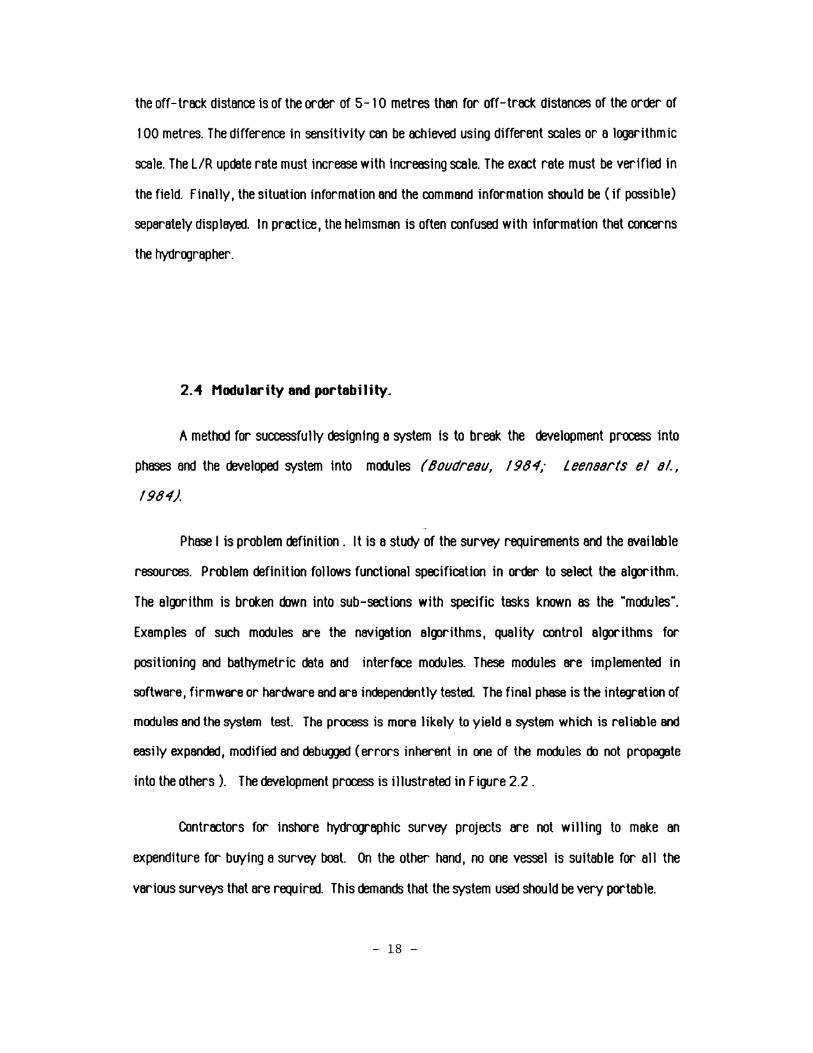
the off-tr~k distance Is of the order of 5-10 metres then for off-tr~ distances of the order of
100 metres. The difference in sensitivity can be ~ieved using different scales or a logarithmic
scale. The L/R update rate must Increase with increasing scale. The exect rate must be verified in
the field. Finally, the situation information and the command information should be (if possible)
separately displayed. In prectice, the helmsman is often confused with information that concerns
the hydrographer.
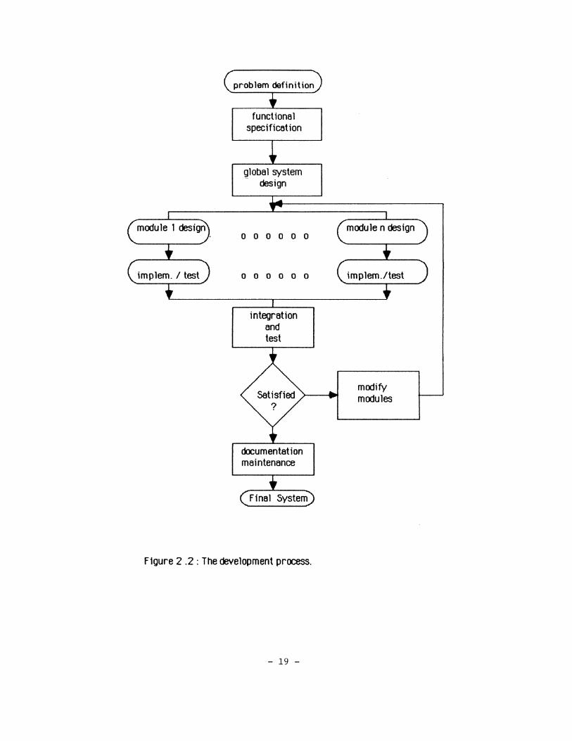
2.4 Modularity and portability.
A method for successfully designing a system Is to break the development process into
phases and the developed system Into mooules (Boudreau, 198"1,· Leenoorts e/ ol.,
198"1).
Phase I is problem definition. It is a stu<ty of the survey requirements and the available
resources. Problem definition follows functional specification in order to select the allp'ithm.
The algorithm is broken down into sub-sections with specific tasks known as the ·mooules·.
Examples of such mooules are the navigation ai!Pf'ithms, quality control allp'ithms for
positioning and bathymetric data and interfece mooules. These modules are implemented in
software, firmware or hardware and are independently tested. The final phase is the integration of
modules and the system test. The process is more likely to yield a system which is reliable and
easily expendad, modified and debugged (errors inherent in one of the modules oo not propagate
into the others ). The development process is illustrated in Figure 2.2.
Qmtrectors for Inshore hydrographic survey projects are not wtlling to make an
expenditure for buying a survey boat. On the other hand, no one vessel is suitable for all the
various surveys that are required. This demands that the system used should be very portable.
- 18 -
functional specification
global system - design
0 0 0 0 0 0
0 0 0 0 0 0
integration and test
documentation maintenance
F1gure 2 .2 : The development process.
- 19 -
modify modules
2.5 Compatibility
Compatibility is the ability of the system to communicate with 8 variety of devices and to
worlc in 8 variety of computer envirooments.
The Wf/1/ that data Is transferred between the different sub-systems depicts its
compatlb11ity. For example, data should be recorded on a standard medium with· compatible
records and not ptd(ed records requiring special assembly language routines to 8::CeSS the data.
The use of standard lnterfl~:es ( RS-232 or IEEE-488 , see /1c Namara ( 1977)) enables the
system to worlc with other standard interf8:8 devices.
The system should use standard hardware, and in the case where special hardware has to
be built, a bus-system organization can be 800pted.
The software should be mfdl1ne independent. This implies that a standard operating
system and language compiler be used from a reputable manuf~turer. Structured and modular
programming contributes to compatibility. Any necessary software transfer to another computer
that requires modifications can be done by changing only specific software modules. Software
transfer or modification can be better done in high level language. Hence, assembly routines
should be lcept to a minimum and only in these parts of the system that are not ~lng to change
during the system-life (e.g. sensor communication routines ).
- 20 -
2.6 Cost
In order to determine the upper limit cost of the system we have to identify the agencies
that require inshore hydrographic surveys and how much they ere willing to pay. As stated in
I 811 repor I ~' I (I 982) these agencies mainly belong to the public sector and are satisfied
with the conventional methods of surveying (e.g. intersecting directions with the:xblites with line
lceeping controlled by one of the theo00lite8). When the volume of survey worlc requires small
amount of manpower these methods are cost-effective. The prop0500 system should be able to
compete with these techniques with regards to cost.
Therefore, a reasonable 1})81 for the navigation controller, not including the positioning
system and the echosounder is $5000 minimum per unit. This includes:
- computer - interface unit and
echosounder digitizer - computer peripherals
TOTAL
$ 1500
$2500 s 1000 $5000
Maximum cost should be S I 0000. This does not include the expense of development and
prototyping. However, it is a cost-effective alternative to present commercially available data
~isitionandprocessing~emssuch as the NAVBOX (Tripe, 1978) and the ATLAS SUSY
30 (F/8, 1984).
It is difficult to give priorities in the above list of design criteria unless the project
requirements and the available resources are exactly known. As previously stated, accuracy has
the highest priority in near shore marine constructions. However, for near shore applications
reliability is not so Important since, in the case of system malfunction, the boot can Immediately
return to shore for repair.
- 21 -

2. 7 Review of existing systems
Some of the concepts ack:lressed in this thesis are not new. The concept of LIR indicator,
the aliJif'ithms to further process the data have been implemented in larger systems while the
emphasis here is the scaling OO'Nn of these systems to a system that will serve the needs for near
shore hydrography and it based on microcomputer technology. Therefore, potential benefits may
be gained by reviewing these syStems and pointing out their limitations and highlights. Their
review and comparative performance evaluation will be done according to the established earlier
in this chapter design criteria
In Csnada, the Csnadian Hydrographic Service ( CHS) is responsible for charting CsmKifan
waters. This responsibility is distributed to the regional offices which have designed their own
acquisition and processing systems. Some regions use computer-assisted techinques for data
processing only. Data is collected ustng conventional manual methods during the day and in the
evening is processed on board the "mother ship". Even within regions some types of survf¥5
(e.g. wharf survf¥5) are not automated and others (e.g. offshore survf¥5) are.
The development of acquisition systems does not follow any standard formats and therefore
the information exchange is difficult. The latest developments include the Integrated Data
Acquisition and Processing System ( INDAPS), the Portable Hydrographic Acquisition System
(PHAS) and the NAYBOX or HY-NAV. The INDAPS system is a mini-computer based system
suitable for launch or major ship fittings. PHAS is a microprocessor based system which like
INDAPS is still in use. NAYBOX is a similar to PHAS system but in ackiition, has navigation
functions. Detailed descriptions of the hardware and software organization of INDAPS can be found
in Brayantetal. (1976) andofNAVBOXandPHAS in Tripe(/978).
These systems are machine language pr(JJrammed and therefore are strongly hardware
oriented. It is difficult, and sometimes impossible, to modify them to meet different user
requirements. This reduces their compatibility with other hardware and software.
- 22 -
In terms of man/mej}lne inter~tlon, cl8te and command entry is 00ne using keybotrd or
keyptl! entry of mnemonic commands; an Inefficient meens of communication especially In the
harsh hydrCJJfaphlc environment. This form of communication is found In all the systems
( INDAPS, NAVBOX and PHAS). The problem worsens when the user wishes to modify the survey
parameters during the survey. The 8bi1ity of the systems to implement different patterns of
survey lines is also reduced. Only straight lines, or lines of position can be surveyed.
At some stage of HY -NAV's development the system was not reliable (Wells, 1983
personal communication). For example, the system had a floating point arithmetic board but
with some algorithm bugs. The depth digitizer used required strong bottom echoes to trip- its
clock mechanism. Aeration, especially in rough seas, produced false soundings. Some temperature
sensitive components resulted in different romputed positions at different temperatures.
The data is obtained from the sensors asynchronously. A one second lag exists ( -3m at
5 knots ) between the position and depth samples and the samples are not correctly correlated
with time. F11terfng techniques (positioning 8lld bathymetric) are Implemented for data
validation but they are not always effecttve. For example, lane jumps are detected In the Mlntnx
phase comparison system by comparing the Jane jumps to the distance trave11ed at maximum
speed. The technique dJes not give the ex~t cycle ambiguity. There is more success, however, in
depth filtering techniques.
The Interact Research and Development Corporation has recently enounced the ISAH
acquisition and processing system. Some of the features of ISAH are:
- Men/machine rommunivation using graphic displays and graphic left/right indicator with
selectable SC8les.
- Hyperbolic, multi-range and range/ bearing algorithms using weighted least squares to
derive position fixes.
- Track and sounding plotting.
- Tide and sound velocity corrections to depth data.
- 23 -

The PEK:ific Region recently announced the development of its own data q.~isition system
with a real time operating and application system supplied by lnterEK:t Research and Development.
Low level programming, high data acquisition speed and no applied filtering techniques are some of
the charEK:teristics of the new !Esign. The philosophy of the design is to record great amount of
data without bothering about quality control as thls wttt delay the EK:QUisltlon process. The quatlty
control task is left for post-processing.
The National Ckean Survey also announced the replfl:ement of the aging HYDROPLOT
acquisition and processing system with Shipboard Data Systems Ill (SDS Ill). Details about
HYDROPLOT system con be found in FIB ( 1911) end Wallace ( 1982) , and details about
SDS Ill system in Enabnit ( 1985). Some of the deficiencies that led to the decision to replace
HYDROPLOT are:
-Virtually all the instruments interffl:ed to HYDROPLOT are asynchronous. The probability
that two tines of position and a depth will all occur at the same time is almost zero.
- Navigation is provided only for parallel straight Jines.
- It is difficult for the hydrographer to "see" the survey data in real time end
take appropriate decisions. This difficulty is found in many other E~:QUisition systems.
In 8(kjition, SDS Ill system has the following features:
- Real time display of soundings and ship's trfl:lcs using colour graphic displays.
- Implementation of a hydrographic data base.
Some other systems that are used In hydrographic syrVf!f<{S, navigation and ott exploration
are NAVPAK ( f"alkenberg, 1981 ), ATLAS SUSY 30, NAVCUBE NC-100 (f"!(J, 1917,·
flO, 1981,· FlO, 1984/) etc .. Although some of these systems are not suitable for inshore
hydrography and dreO:Jing operations, concepts like path guidance and position filtering are
common for near shore and off shore applications.
Here is a summary of the different approaches that have been fd)pted, the unsolved or
controversial problems in data acquisition systems:
- 24 -

1. The proper distribution of d8ta processing functions between on-line 8fld off-line
computers produces differences In opinion.
2. Computers are now widely used in d8t8 acquisition systems to telce advantage of their
ability to provide a navigation function and data processing capabilities such as error detection and
filtering. Systems that employ dedicated microprocessors are not flexible. What is absent (at
least in the CHS) is a m(QJler, software oriented design based on the rapidly developing
microcomputer technology.
3. The majority of manufacturers have Eg'eed to stand8rdize 1/0 (Input/OUtput)
operations and create flexible systems. The old practice of providing BCD (Binary CoEd Decimal)
output has resulted In fi:Qtlisitton systems with many large cables and troublesome connectors.
But the area of 1/0 interfaces is the only one tn which standardization has been 8chleved.
Standardization should include all other mooules of the survey system such as navigation
al!J)rithms and software languages.
4. The correlation of data from various sensors is a reel problem. An "intelligent
interface" is needed to reduce the data to a common digital format and time instance.
5. The requirement to obtain reliable depth data tn digital form remains as one of the
biooest problems In automatic hydrography. This Is reflected in the different approaches th8t are
now ln use 8fld the great activity in this field. The reasous for this wlll be discussed ln chapter 3.
6. Man/machine interaction is not efficient. System operators may normally be people
with little training in computer science or in hydrographic operations. The software should be
able to reflect possible operator's errors by proiucing unambiguous error messages.
7. Straight line navigation is not always an efficient way of sampling depth as will also
be discussed in chapter 3.
- 25 -
If automatic data acquisition systems are empl~. a suitable processing system Is
required that wm handle digital data. Two groups of processing functions are necessary:
-General data orocessina. This includes computation of grid or geographic coordinates,
application of monitor corrections or propagation corrections to improve the quality of position
data, adjustment of soundings for speed of sound corrections, adjustment for water level or heave,
filtering, smoothing, interpolation or-extrapolation of data, detection of shoals and generation of
statistics. This is not a complete list.
- Processing for presentation of results. This Includes selection of representative
samples, plotting, generation of profiles, volume computations etc ..
It is not pra::tical to use the on-line computer to EKX:Oillplish an these tasks, except
perhaps in the case of large shipboard installations such as INTERPLOT 200 survey system
manufactured by INTERSITE Co. (FlO, 1984). For inshore hy(i'ography and marine
engineering, where a small lightweight system is used for acquisition, a small portion of
functions in general data processing is EKX:Oillplished on-line. The rest of processing is mne
either on the same computer off-line or on a larger computer which will handle data from several
acquisition systems such as in the system INDAPS used by the Canadian Hydrographic Service
(Bryant et a/. , 19 76).
- 26 -

J. DATA ACQUISITION and ON-LINE PROCESSING
3. 1 Oenaral systat11 configuration
We wm now elaborate on the previous two chapters to functionally specify an Ideal data
~D:JUisition system.
The distribution of data processing functions is such that ~K::qUisition, navigation and some
of data validation is performed on-line, while the rest of processing is 00ne off-line. By aoopting
this arrangement we overcome some of the disadvantages of complete on-line processing : tidal
heights are not available (unless they are transmitted to the survey boat by a radio link) and a
sophisticated and expensive system is required. The launch equipment used with off-line
processing is simpler and inexpensive. The disadvantage of this approach lies in the requirement
to accurately record large amounts of data for post-processing. However, since all the data is
available we can employ any data reduction technique to satisfy users with varying requirements.
The components of such a hydrographic acquisition and navigation controller are shoWn tn
Figure 3.1. The selection of the appropriate components for inshore hydrographic surveys must
follow the established criteria.
- 27 -

positioning system
sounder system
operator
C.P.U.
displays
hard copy
optional
Figure 3. 1 : Block diagram of a navigation and hydrographic data acquisition controller.
- 28 -

In the remainrer of this section we discuss hardware consirerations, and the structure for
an idealized software package. later in the chapter we deal with details of the software.
3. I. 1 Position Input
Positioning systems that use microwave techniques, such as the pulse matching systems
Motorola Mini Ranger and Del Norte Trisoonder. satisfy the criterion of accuracy for inshore
surveys. These systems provide metre order accuracy. Higher accuracy can be achieved (near
shore) by range-bearing position fixing systems such as Atlas Polarfix ( 30 em at I km far from
shore) (Wentzell, 1985). Recently, Racal Positioning Systems ltd. announced a pulse
matching microwave system of submetre accuracy ( Teunon , /985).
The 61ob81 Positioning System (aPS) is a new satellite based positioning system that is
expected, by the year 1987, to provide continuous two-dimensional navigation which is sufficient
for many marine applications (general navigation, off shore surveys etc.). However, at present
the system is unable to satisfy the accuracy requirements for inshore surveys. In ship trials
conducted by M8J08VOX (Eastwood, 1984), the Magnavox T -Set ePS receiver, when compared
with Trisponder, gave stanmrd deviations of fix differences of the order of 20 metres.
furthermore, the U.S. Department of Defence is planning to deteriorate the accuracy of the system
for civil use. One Wfl'l to recover this accuracy or Improve it, is to use Differential GPS. The
basic concept Is to locate a ePS monitor station at a known benchmark, observe ranges to
satellites, compute corrections to the ranges or positions and transmit them to the local users.
Stansell ( 1984) SfJ1S that the method can give position accuracy better than 5 metres.
Therefore, with Differential 6PS it is possible to meet the ED::Uracy requirements of inshore
surveys and at the same time minimize the labor cost required by the present positioning systems.
However, hydrographers would have to rely on the decisions of U.S. Department of Defence about
the released accuracy.
- 29 -
for SEAHATS, we limit ourselves to considering the Mini Ranger system as the
positioning system. This imp lies that the Input data will consist of ranges to a number ( 2-4) of
control stations on shore.
3. 1.2 Depth input
For inshore applications the echosounder should be chosen to give a high oofinition
echogram of the "first" bottom. The requirements of~ depth resolution, small beamwidths and
small transducer sizes are satisfied only with high frequency transmissions ( 11acPhee, 1919).
Selection criteria for bathymetric systems can be found in Raytheon ( 1984). Watt
( 1911) justifies the use of 30-200 kHz echosounder with beamwidths 2.5-10 00grees and
pulse duration 0.1-0.5 milliseconds.
for SEAHATS, the Slmrad Skipper 802 echosounder with 50 kHz transducer is chosen to
provioo depth input.
3. 1.3 Central Processing Unit
The requirements for the central processor include low cost, low power consumption, bus
oriented structure for flexible 1/0, and the ability to work in a standard operating system
environment like CP/M or DOS, allowing the use of "off-the-shelf" compilers like BASIC and
PASCAL. Features like DMA (Direct Memory Access) and 16 or 32 bit word lengths are
desirable. DMA will permit fast output of collected soundings to the logging device without
stopping the navigation functions. Larger word lengths will permit access to larger RAM than 64
kbytes. The mass storage device should be able to store at least 3-4 hours of survey data ( 150
kbytes typically).
- 30 -
for SEAHATS, the Apple lie microcomputer has be chosen as the CPU. Apple lie is based
around the 6502 microprocessor and it has 8 expansion slots for 1/0 devices and other
peripherals. In general, Apple lie ooes not support interrupts from 1/0 devices although the 6502
microprocessor has an interrupt pin. However, with user written programs the Apple lie can be
mooifieed to support one 1/0 Interrupt. The Apple lie microcomputer has not a DMA feature.
3. 1.1 Acquisition software
As mentioned in section 2.4 the development process is broken into modules. for
SEAHATS, the following modules were implemented:
- INITIALIZATION,
- INTERFACE,
- QUALITY CONTROL,
- NAVIGATION,
- ON-LINE MODIFICA.TION and
-OUTPUT.
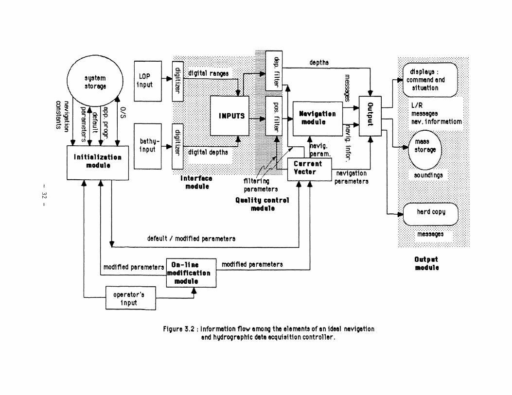
Figure 3.2 illustrates the information flow between modules.
The INITIALIZATION module is responsible for laooing the Operating System, application
pro;)rams, default parameters and navigation constants from the system storage. The default
parameters are the latest navigation parameters that were in use. It also accepts operator's tnputs
and selects the navigation function (shoal examination, primary survey lines and Wflf potnt
navigation ) 1.
The purpose of the INTERFACE module is to convert the inputs (LOPs and depth) to digital
form and provide data to the navigation module. Between the interface and navigation modules, the
1 they will be discussed in section 3.4
- 31 -
w N
I nttialtzation IBodUla
LOP input
bethyi nput
default I modified parameters
1 modified pare meters I On-lt ae 1 modified parameters ..... _____ __,_medtflcatton
operator's input
IDOdule
depths
lavtgatten module
fiQure 3.2: Information flow amon9 the elements ofen ideal navtget1on end hydroQraph1c dete acquisition controller.
displays : commend end
situation
Outp•t .. dule
QUALITY CONTROL mOOllle Is responsible for f1ltering position and bathymetric data. The task of
the NAVIeATION module is to compute the vessel's position and translate the positton fnformat1on
to a form famfllar to coxswafn and hydrOJrapher. The OUTPUT module will display steering and
navigation information, log positions and depths with their statistical characteristics.
The bus with which the above modules communicate is the CURRENT VECTOR (Boudreau,
1984). It contains the survey parameters which are effective during the running of the survey
lines. These parameters are :
- the survey function selected ( shoal examination, primary survey lines or Wfftl point
navigation) with the specifications of 1 ines (line spacing, maximum leg length ) ;
- the ww points selected to defined the system of lines to be run;
- the control ooints used;
- rates used - sampli.ng data rate ( ranges to transponders and depths)
- position update interval
- lQIJ.Iing rate
- printing rate
-display update rate (for skipper)
- display update rate ( for hydrographer);
- firm for - lQIJ.Iing data
- printing data
-minimum depth ( to prevent grounding);
- filter parameters for position and depth validation and
- file names used for storing survey data or default parameters.
The content of the current vector is modified either off-line in the initialization
procedure or on-line (while running survey lines) through the ON-LINE MODIFICATION mOOllle.
The elements of current vector can also be specified laooing the DEFAULT file. Its structure is
- 33 -

similar to the structure of current vector and resides on a non-volatile medium. Upon completion
of survey work the Off AUL T file is automatically updated.
The rest of this chapter is devoted to an in depth analysis of INTERFACE, QUALITY
CONTROL, NAVIGATION , ON-LINE MODIFICATION and OUTPUT modules. The part of OUTPUT module
that deals with man/machine interaction was discussed in section 2.3 .
3.2 The INTERFACE module
We describe the interface environment necessary for inshore hydrography. At least two
sensors are involved : the echosounder and the positioning system. Their outputs 'should be
computer compatible. All electronic positioning systems, used in the line-of-sight area,
currently provide digital positioning data either in BCD format or through an RS-232 serial
interface. Unfortunately, no depth sounder has been designed as a truly digital sounder. A special
device, called "the digitizer", is needed to convert analog depth signals to digital form.
The digitizer computes depth using equation :
DEPTH= ( 112) n T V8 (3.1)
and counting the number of cycles ( n) of a crystal controiJed oscillator (period T) during the
travel time of ocoustfc pulses fn sea water. The assumed sound velocity fs V s· for shallow water
systems, where there is only one pulse in the water at any one time the implementation of this
equation is straight forward. For systems used in deep waters however, groups of pulses are
transmitted and there must be some programmed logic controlling which pulse wi11 signal the
digitizer counter to stop. Details about depth digitization can be found in Thomson et al.
( 198/) and Raytheon ( 1984).
- 34 -
The rates at which digital LOPs and depth dBto 8f'e provided by the positioning and sounding
system are different. A high depth rate is necessa1 y to accurately represent sea bottom
topo;Jraphy since sea bottom hos an unpredictable behaviour. Also, the filtering techniques
described in section 3.3 require high dBta rates. Echosounders used for shallow waters (depths
less than I 00 metres) can give soundings at a rate of I 0 soundings per second (see 11acPhee,
1919). This rate is ~ate provided that iL is available for fNerY second. Hardware
constraints, however, may prevent soundings from being read when the computer is busy doing
computations or recording dBta.
On the other hand, the movement of the ship is well predicted for short periods ( 2-3
seconds). Range sampling rates of I per second are ~uote to describe ship's kinematics for
inshore surveys.
Bosically there are two approoches to Input bathymetric 8nd positioning dBta to the
computer (see Short, 1981):
I. PrD]'am Controlled Input/ OUtput.
2. Interrupt Controlled Input/ OUtput.
With the program controlled 110, the microcomputer initiates the transfer of dBta by
cycling through the sensors as illustrated in Figure 3.3 . A real time clock has been ackjed to the
list of sensors to provire the time of day. Sometimes it is necessary to check if the sensor is ready
to provide dBta by Mpolling". Polling a sensor consumes a significant amount of microprocessor
time. Time delays are introduced and therefore position and bathymetric data is no longer
correlated. Program controlled 1/0 does not efficiently handle asynchronous data transmission
and large data streams.
Hardware interrupts can be used to overcome these obstacles. The computer responds to
the Input deVices when they have dBta. Each deVice hos its own interrupt service routine and
priority level. Figure 3.4 illustrates an interrupt driven input/output layout.
- 35 -

compute, display , log
Figure 3.3: A program Contro11ed Input/ Output.
compute ,display log, print
interrupts
Figure 3.4: An interrupt Controlled Input/ Output.
- 36 -
LOPs
depth
time
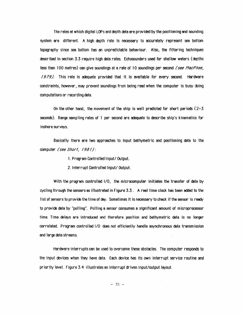
The need for interrupts of the central processor may be avoided by using an "intelligent
interface" provided that it has sufficient intelli~ to chronologically correlate positioning and
bathymetric data. The interrupt function is still there, but allocated to a separate processor, in a
distributed processor architecture. The central processor can then ~ only buffers, provided
by the peripheral processors. The ultimate extension of this distributed architecture is building
the peripheral processors Into the sensor p~ages (the sensors have a buffered output).
The "intelligent interface" may serve other purposes such as the reduction of data to a
common format. An example of one such interface is the JMR marine data acquisition and
navigation system (SYSTEM 21) ( J/1/l, /981). The electrical and functional operation of
the interface should be standardized. By electrical operation we mean the electrical interface used
(e.g. RS-232 or 20 mA current loop). The functional operation is the regulation of the flow of
data between the sensors and the central processor. For the particular application, a basic
functional operation is described by the following communication protocol :
START : Start receiving ranges and depths at equally spaced time intervals and store them
in a local buffer.
REQUEST: Request a data point from the local buffer.
STOP : Stop taking samples.
Figure 3.5 illustrates the use of an "intelligent interface" for hydrographfc purposes.
Hydrographic data must be stored in digital form for further processing. Underway
recording should be fast and correct in order not to delay the acquisition process. DMA (Direct
Memory Access) is an appropriate fast data transfer mechanism, provided that the microprocessor
has a DMA feature. The Apple lie computer for example, dJes not have direct memory~ for
its disk controller and must stop everything else while it reads or writes information on the disk.
During this time information from keyboard or other 1/0 device is lost.
- 37 -

communication } protocol
Intelligent interface
buffer
compute, display log, print
F1gure 3.5: An "1nte111gent" interface.
- 38 -

The need for valid recording of acquired data is vital in order not to lose data due to
"electrical noise" that exists in hydrographic vessels. It is not sufficient to only detect an error,
it must also be corrected. Procedures used in automatic hydrographic data acquisition systems to
validate recorded data are (from FIB, 198 I) :
(a) methods to validate d8ta before the writeheOO:
-Parity check;
-Cyclic Redundancy Check (CRC) and
- Redundant storage (same data written two or more times);
(b) methods to detect errors that occur while performing a reOO or write operation:
- REB~ after write with error flag and
- RM:I after write with re-write.
Cyclic Redundancy Check is an error detection method that provides multiple bit error
detection in serial data transfer while parity check cannot. Details on error detection techniques
can be found in /1c Nom oro (I 9 7 7). The majority of the systems use either parity check or
CRC to detect an error before the writeheOO and re-write the data when an error occurs. Cyclic
Redundancy Check is a common method of error detection for serial data transfer in systems using
floppy disks such as the Apple lie microcomputer. It seems to perform well in the electrically
noisy environment of hydrographic launches.
For SEAHATS, the Intelligent lnterf~ approoch was taken. The spectflc tnterf~ used
was specially developed for SEAHATS, and is called the PS-0 1 (for Parallel to Serial
converter). Details are given in Nickerson ( 1983).
- 39 -

3.3 The QUALITY CONTROL module
3.3.1 Nature of positioning errors
Before we try to monitor the errors inherent in microwave systems we have to examine
the nature of these errors, particularly for pulse matching 5Ystems such as Del Norte Trisponoor
and Motorola Mini Ranger. This error buD;Jet is 0011e occording to the welll<nown classification in
rarnX!m, systematic and gross errors, although it is difficult to draw distinct boundaries between
the classes.
These 5Ytems measure the travel time of pulses, from remote transponders to the
Receiver/Transmitter antenna mounted on the ship, without phase comparison techniques. Figure
3.6 shows the typical forms of transmitted and received pulses. The factors that affect the
accuracy of time measurement are: the noise that deforms the leading edge of transmitted pulse,
the threshold level variation and the instab111ty of Mini Ranger clock osc111ator.
Random Errors: Tests mooa (Tripe et 81., 1914,· CBsey, 1981) demonstrate
that random errors in Mini Ranger system are normally distributed as a sum of two normal
distributions with zero means but different variances. One has a standard ooviation of 2 to 5
metres containing the majority of the readings and a second with standard ooviation 5 to 15
metres containing the remaining values (figure 3.7). The r8n00m process responsible for the
first originates from the slight variations occurring naturally within the system such as clocl<
instabtllty and variations on threshold level. Signal to noise ratio accounts for the second
distribution. In microwave systems ( 300MHz<f<3006Hz), the detailed structure of the
atmosphere becomes important and therefore, the signal to noise ratio decreases as the beam is
scatterred by rain or hail particles (HBII, .1979). For the frequency used in Mini Ranger
( 5480 MHz ) , the attenuation due to the energy absorption by rain drops is approximately 0.2 dB
per l<m. The instantaneous signal level is also a function of distance, pointing of the antenna, as
well as roll and pitch of the vessel that alter the effective gain of the antenna.
- 40 -

Systematic Errors: When the signal level is above the threshold the relationship between
range error (due to roouced signal to noise ratio) and distance is prooictable. This relationship is
describoo by the ra1ar ~ation ( L aur ila, 1916) which says that, if we isotropically
transmit a power Pt with an antenna of gain a, the power we receive at a distance R is: aPt I R2.
The signal to noise ratio is therefore inversly proportional to the square of distance. With
rOOuced signal to noise ratio the Mini Ranger 5)'Stem has difficulties in discriminating the lea:ling
00ge of the pulse in Figure 3.6, and this results in a positive range error proportional to the
square of distance. Casey ( 1981) shows these results experimentally. This error can to
some extent be eliminatoo.
Zero error, caused by signal delays inside the electronics (e.g. Receiver/Transmitter
cable induced delay) can be removoo by proper calibration. For microwave 5)'Stems, atmospheric
refractivity varies with the velocity of radio wave propagation. Deviations from the assumed
speed of light (refractivity Ns=320) are given by Smith-Welntraub or Essen-Froome formulae
( L sur ila, 1916). The range errors are relatively small e.g. 0.20 metres at 1 0 km .
aross Errors: Multipath propagation causes serious problems to microwave positioning
systems. Reflections from rock faces or ship hulls can cause range errors up to hundred of metres
(Tripe eta/., /914). The Mini Ranger 5)'Stem has a feature to detect these reflections and
sets the rea:lings to zeros. Unfortunately these zero rea:lings can appear as gross errors to
automatic 5)'Stems which do not have a zero range software detection technique. When geometry
permits, the direct signal arriving at the receiver and the signal reflected from the water's
surface Interfere with eech other resulting In signal cancellation and no range rea:ling. This
phenomenon is calloo a ·raooo hole" and is very common In hydrographic surveys using microwave
techniques. tJi/b et a/. ( 1916) describes this phenomenon and gives methOOs to avoid its
occurrence. Mainly, these methods are practical and are not suitable for an automatic data
ocquisition system. The following two methods can be use in an automatic system:
(a) To use two Receiver/Transmitter antennas at different elevations. The automatic system wm
- 41 -

pulse amplitude (volts)
c: 0 --., transmitted pulse received pulse 1: ., :> -.; 1 l; -'"0
0 .c. of) time e L -.c. - 0.3 microseconds clock instability
Figure 3.6 : The forms of transmitted and received pulses 1n M1nl Ranger.
P(x)
N(0,2):fl(x)
7 N(O,S): f2(x)
0 X
P(x) =a fl(x) + b f2(x) with a» band a+ b= 1
Figure 3.7: Random errors in Mini Ranger.
sea surface
p -(~ J - air bubbles
Figure 3.8 : A typical echogram.
- 42 -
switch between the two antennas oopending upon the strenght of the signal from ~ antenna.
(b) To morel the Mini Ranger range time series as discussed in section 3.3.3.
Mini Ranger ckles not suffer from cycle ambiguities, as it ckles not use phase comparison
techniques.
3.3.2 Nature of bathymetric errors
The nature of bathymetric errors is slightly different from that of positioning errors.
Figure 3.8 is a typical analog tr~ of echosounOOr'. Interpreting the echogram we notice the
following:
The sawtooth effect Is normally caused by the rolling, pitching and vertical motion of the
vessel (heave), or 1t Is a picture of sea bottom that has undulations of slm11ar order. Roll, p1tch,
heave effects can to some extent be mOOelled, sensed and corrected (Hopkins , 1980). In
oo:Jition to the seabed, the echosounOOr also receives renections from fish, wrecks, seaweed and
air bubbles in the water which are called false echoes. The human eye is a perfect filter and can
easily distinguish between seabed and false echoes on the tr~. But the use of on-line oopth
digitizers invariably digitizes a percentage of false echoes along with the valid soundings. As a
result, procedures are required to ootect these errors and 1t ts usually necessary to compare the
digital soundings directly with the echogram. Hence an important feature of the digital system is
the capab111ty of producing a plot from the dlg1tal cleta that can be OOjusted tn time and OOpth scales
to exoctly match the analog troce on the echogram.
Differences in the speed of sound in sea water can cause systematic oopth errors of the
order of decimetres. These errors and others associated with echosounOOr instr-umentation (stylus
- 43 -
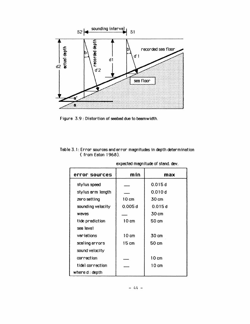
52 1• sounding interva~ 51
.... d2 ~
Figure 3. 9 : Distortion of seabed due to beam width.
Table 3.1: Error sources and error magnitudes in depth determination ( from Eaton 1968).
expected magnitude of stand. dev.
error sources min max
stylus speed - 0.015 d
stylus arm length - 0.010 d
zero setting tO em 30cm
sounding velocity 0.005 d 0.015 d
waves - 30cm
tide prediction 10 em 50 em
sea level
variations 10cm 30cm
scaling errors 15 em 50 em
sound velocity
correction - 10cm
tida 1 correction - 10 em
where d : depth
- 44 -

speed, stylus-arm length, zero setting etc.) can be removed by proper calibration (t/mbtJch,
19 76,· Thomson et tJI., 1981).
Other sources of errors in the determination of depth ere errors in tide prediction and
abnormal variations in water level (due to atmospheric pressure differences or wind effects).
Also, sampling a seabed with steep slopes results in distortion of the actual depths and slopes due to
the beamwidth. It can easily be shown that the recorded depth and slope ere :
d' = ( cos( a) I cos( a-b)) d, a'= arctan (sin( a) I sin( a-b)) (3.2)
where: a, d actual slope and depth; a·, d' recorded slope and depth and b= 112*beamwidth (see
also Figure 3. 9). A direct consequence of this is the hyperbolic presentation of peaks on the see
floor.
If we exclude false echoes and the effects of beam width, Table 3.1 gives an indication of the
magnitude of the above errors (EtJton, 1968).
3.3.3 Quality control of positioning data
The filters that ere widely used in hydr()Jraphic surveys to derive ~rate positions from
noisy range observations are the time domain filters:
-Gating (or screening);
- Least Squares ( multtrangtng);
- Least Squares curve approximation (with fixed or expanding or fading memory); and
- Kalman filter.
- 45 -
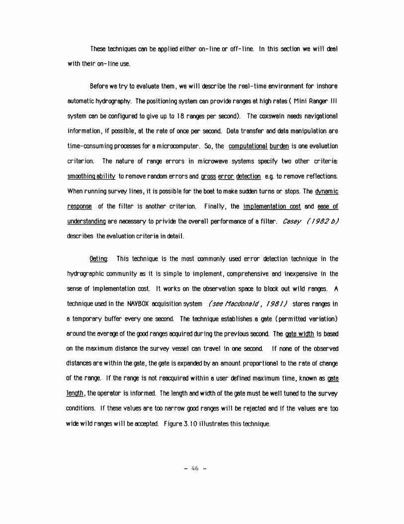
These techniques can be applied either on-line or off-line. In this section we will deal
with their on-line use.
Before we try to evaluate them, we will describe the real-time environment for inshore
automatic hydrography. The positioning system can provide ranges at high rates ( Mini Ranger Ill
system can be configured to give up to 18 ranges per second). The coxswain needs navigational
information, if possible, at the rate of once per second. Data transfer and data manipulation are
time-consuming processes for a microcomputer. So, the computational burden is one evaluation
criterion. The nature of range errors in microwave systems specify two other criteria:
smoothing ability to remove random errors and gross error detection e.g. to remove reflections.
When running survey lines, it is possible for the boat to make sudden turns or stops. The atnamic
response of the filter is another criterion. Finally, the implementation cost and ease of
understanding are necessary to privide the overall performance of a filter. Casey ( 1982 b)
describes the evaluation criteria in detail.
eatina: This technique is the most commonly used error detection technique in the
hydrographic community as it is simple to implement, comprehensive and inexpensive in the
sense of Implementation cost. It works on the observation space to block out w11d ranges. A
technique used in the NAVBOX EK:QUisition system (see 11acdonald, 1981) stores ranges in
a temporary buffer every one second. The technique establishes a gate (permitted variation)
around the aver~ of the good ranges EK:QUired during the previous second. The aate width is based
on the maximum distance the survey vessel can travel In one second. If none of the observed
distances are within the gate, the gate is expanded by an amount proportional to the rate of change
of the range. If the range Is not reacquired within a user defined maximum time, known as ~
lenath, the operator is informed. The length and width of the gate must be well tuned to the survey
conditions. If these values are too narrow good ranges will be rejected and if the values are too
wide wild ranges will be ~ted. Figure 3.10 illustrates this technique.
- 46 -

Multiranging: The use of multiranglng is restricted to ranges from one positioning
system. It is difficult to estimate the relative weighting to be given, especially in real time, to
different systems (Weeks, 1982), particularly if these systems use different measuring
techniques (e.g. phase comparison or pulse matching techniques). Therefore, the use of least
Squares is llmlted to 3 or 4 LOPs from one type of sensor. The redundant ranges, Increase
expenditures, time and labor cost. However, redundant ranges permtt real time error detection
and prevent the need for having to resurvey or detailed checKing of data. Various authors have
~ressed the di5tKNantfqlS of multiranging as the filtering technique to detect wild ranges
(Bergen, 19 79,· Cosey, /982o,· Eoton, 1982). It may have a zero response time 8nd
inform the user for a poor fix, but it dles not have any spik.e detection ability (at least for 3
LOPs). These are 11mttat1ons to the main advantage of multtranging that no alternative to
multiranging provides error detection without any assumpions.
Least Squares curve approximation : Another way of deriving ~rate positions is to
approximate the range time series by a polynomial. We may implement an expanding or fixed or
fading memory filter. However, expanding filters (recursive or not) may give systematic errors
that grow very rapidly. For details concerning fixed, expanding, and fading memory filters see
11orrison ( 1969).
Suppose we want to approximate the Mini Ranger range time series (shown in Figure
3. II) using a fixed memory filter. The observations are equally spaced in time. The number of
observations that w111 be used (memory length : L) the degree of polynomial ( m) must be
carefully chosen In order to balance systematic and random errors. Systematic errors arise
from the fact that the chosen polynomial may not match the true range time series and random
errors have their origin to random errors in the observations. The following should be Kept in
mind. Details can also be found in 11orrison ( 1969):
- By increasing the degree of the filter the systematic errors are reduced. However, as we
increase the degree, the variances of the random errors increase.
- 47 -

station
gate width = 2 dt Vmax (metres)
gate length = L (seconds)
survey line
Figure 3. 1 0 : Gating technique to detect range spikes.
Range
true range process
1 2 3 4 5 6 7 8 9 10 11 12 13 1415 n memory length L = 5
Figure 3. 1 1 : The fixed memory range filter.
- 48 -
- When the length of memory increases the systematic errors increase but the variances
OOcr'ease.
Casey ( 1982b) shows that Mini Ranger ranges are locally linear for short time
intervals ( 2-3 seconds). This is probably due to the design of the range tracking filter built into
the receiver. Also, it depends on how the vessel is being used; running straight lines is likely to
result in linear behaviour of the ranges. So, the range process can be approximated by the linear
filter (see Figure 3.11):
R = b0 +bJ(nt) (3.3)
For memory length L=5 ( Rn.Rn-I.Rn-2·Rn-3.Rn-4) the n+l predictedrangeisgiven:
Rn+ 1 = 1/10 ( 8Rn + 5Rn-1 + 2Rn-2- Rn-3- 4Rn-4)
and the rate of change :
b1 = 1/1 ot (2Rn + Rn-1 - Rn-3- 2Rn-4>
(3.4)
(3.5)
where: t is the sampling interval (e.g. 0.5 seconds). 11orr ison ( /96 9) gives the general
forms for degree ( m) and memory length ( L ).
Casey ( 1982b) also shows (using simulation techniques) that this type of filter has
good statistical efficiency and !t(namic response equivalent to that of the Kalman f11ter {see figure
3.12). The form is easily programmed and can be used to predict the next range reading. If we
specify a maximum difference between predicted and observed range (gate width), the filter is
similar to the .gating technique described earlier. However, the computational burden is
increased If the observations are not equally spll:ed In ttme.
Kalman filtering: If we know the dynamic behaviour of the ship with its statistical
characteristics, we can incorporate this knowledge with range observations and their associated
statistics to improve our fix. This technique, known as Kalman filtering, implies the use of a
"dynamic" model to describe the ship dynamics and an "observation" model to relate the "state
vector" with the observations. The formulation of these models and the derivation of normal
equations can be found in fJrant ( 1976), Schwarz ( /983) and fJelb ( 1974).
- 49 -

-., C) L -C)
E -., C) 0' c 4D .... -0 c 0 ~ -., > C) '0 '0 L ., '0 c ., -.,
-., C)
!; -6 ., E - -4
-2
2
6
0
Unfiltered
'- . ""-.
Fixed memory '-.. ---------- ----·-- ~.- ---- --·
Kalman
.2 .4 .6 .8 1. fode rete (f) (a) statistical efficiency
(b) fllter response \n high speed turn ( 180 degrees)
Figure 3. 12: Statistical efficiency and dynamic response of range filters (from Casey, 1982).
- so -
seconds
However, there are a number of draw-backs in Kalman filtering that oo not permit its
implementation in the acquisition system studied here. These include:
1. It carries a heavy computational burden.
2. The filter is very sensitive to the existence of outliers in the system noise statistics.
As mentioned erlier, in microwave systems, the occurrence of outliers in range observations
(reflections'from rocks, range holes etc.) is very common. The Kalman filter will only control
the ranoom errors of the Mini Ranger system. Janes ( 1983) gives a qualitative performance
of filter robustness against moceland observation noise statistical characteristics.
3. It is extremely sensitive to variations from the true {}fnamic mocel.
We must always keep the raw data and not alter it with a f11ter which might have not been
the appropriate filter for the particular application.
From Figure 3.12a we see that the f~ing memory filter has a~ statistical efficiency
for f~ing rate f > 0.98. We also see that, for this f~ing rate, it has a very poor {}fnamic
response (Figure 3.12b). For such values the induced systematic errors are large.
For SEAHATS, range spikes are retected in reel time by using a gating technique. The
gate width is based on the maximum distance the survey vessel can travel between range
observations. In fd1ition, provision for multiranging has been mare in the software. After
eliminating range spikes in reel time, a simple Kalman filter is used to post-process the ranges.
The filter can be tuned to reflect the actual survey conditions (range stabil1ty, vessel's
accelerations etc.). This filter is discussed In section 4.3. 1.
- 51 -

3.3.1 Quality control of bathymetric data
The only Wff{ to control errors caused by beamwidth is to use narrow beamwidth
echosounders. In this section we focus on procedures to eliminate digital false echoes. Eech
digitized depth in order to be reliable, hes to successfully pass the following tests:
1. test for valid format and
2. to be inside a tracking gate (gating technique).
Test 1 is performed easily. The gating technique is difficult to use. It has to be well
tuned to the survey conditions (sounding speed, bottom type, semp11ng rate) to be effective. If
the majority of false echoes are caused by aeration or surface reverberation, these echoes cen be
eliminated by testing them against a minimum defined depth. The minimum depth should be
cerefully chosen not to conflict with the shallow water alarm used to prevent grounding. If the
echosounder does not trldc the bottom and produces deep depths (that equal the deeper limit of the
echosounder range selector switch) these depths cen be eliminated by testing them against a
maximum defined depth.
The gating technique used in NAYBOX system ( 11acdonald, 1981) establishes a
permanent aate around an accepted depth that has a user defined aate width. If the next depth falls
inside this gate, the gate is re-established around the new depth. If a depth is outside, a
temporary oote is established around it. If a number of subsequent depths (the number is
specified by the user and it is known as the aate length) falls within the temporary gate, this gate
becomes permanent and all the depths are ta:epted.
The gate length end width have to be selected carefully. If the gate length or width are too
small, echo returns from steep slopes or wreclcs will be excluded; when it is too large the error
rate will inevitably increase. The selection of gate length and width is based on the type of bottom,
boat speed, weather conditions and sounding rate. If the maximum seabed slope to be recorded Is I
- 52 -

( regrees) the sounding rate is r (soundings/sec) and the ship's speed V( m/sec) I the gate width
(g) should be:
g >= (2V/r) tan i (metres) (3.6)
The minimum gate length ( L) that will record echoes from seabed features similar to those shown
in Figure 3.13 will be
L = 8max r /V >= I (3.7)
where amax =maximum length of feature to be recorded.
Another wey to checlc digital depths is to visually compare them with the echo;Jram. Some
means of correlating digital and analog depths must be devised. One wey is to transmit time maries
to the analog trt~:e. A better wey is to convert digital depths baclc to analog and displey them
simultaneously with the original analog depth record.
The above filtering techniques can be implemented either in software or hardware. For
SEAHATS 1 the quality control of depth observations is done in software while post-processing the
ocquired data. False echoes are detected by displsying depth versus time at the same scale as the
echogram and visually comparing digital and analog plots (see section 4.5).
3.4 The NAYIOATION module
The vessel's position is usually found by measuring ranges to a number of known points.
The procedure required to compute the ship's coordinates and provide steering information is:
( i) to project the measured distances onto the chosen coordinate system I
( ii) to 9Jffipute the position and
(iii) to compute the navigation information (e.g. off-trock distances).
- 53 -

- g/
Figure 3. 13: The sea bottom tracking gate.
rejected -
Figure 3. 14: The sequence of tasks needed to apply a scale factor.
- 54 -

There are two routes to follow in order to oo steps ( i) 80d ( ii). The first route is to
reduce the observed ranges onto the reference ellipsoid, use e1Upsoid81 computations to find
geroetic coordinates end project these coordinates onto the mapping plane. The second route is to
reduce the observed ranges onto the reference ellipsoid, multiply them with a SCBie f~tor and use
plane trigonometry to compute grid coordinates. In pr~tice, the second route is preferable
because it saves large amount of computer execution time. Finally, the navigation information
(step iii) is computed using plane trigonometry, provided that the Wflf point coordinates are
referred to the seme coordinate system 8S ship's coordinates.
For inshore surveys the above procedure can be simplified. L aur i/o ( 19 76) gives the
formulae to reduce observed ranges to the reference ellipsoid. The estimated correction, for short
ranges near the sea surfoce, is negligible. For example, if we measure a distance of 30 km
between two points with elevations 1 0 and 1 00 metres and assume a coefficient of refr~tion
k=0.16, the correction is only -0.602 metres. However, we cannot ignore the scale f~tor
computations. For example, if we are working in the vicinity of central meridian of a U.T.M. grid,
where the SC81e f~tor is k0 =0.9996, and fail to apply the SCBie f~tor to observed ranges, our
ranges will be 30000 X 0. 9996 = 12 metres in error.
Cross ( 1981) gives the approximate formula to compute the SC8le f~tor on a given
point P, developed by Redfearn in 1948:
where:
M/M0 = 1 +0.5(E/R)2 +( 1/24)(EIR)4( 1 +4 e cos2cp)
M0 : SC8le factor on central meridian
M : SC8le f~tor on point P
E : Eesting of point P
N : Northing of point P
e :square of second eccentricity of reference ellipsoide
cp : latitude at which the ( N/M0 ) equals the meridional distance
- 55 -
(3.8)
R2 = M02pu at latitude cp and
p, \J: meridional and prime vertical radii of curvature.
Given the points 1 and 2, to compute the scale factor applicable to the line joining them we
compute the scale factor at the mid point of the line:
M12 = Mmid (3.9)
or integrate numerically by Simpson's rule:
M12 = 1/6(Mt+4Mmid+M2) (3.10)
Bamford ( 1962) shows that by using equations (3.8) and ( 3.1 0) the error in the line
length can not exceed 0.1 ppm. Formulae ( 3.8) and ( 3.1 0) are therefore satisfactory with regard
to ~uracy. In practice, the algorithm showed in Figure 3.14 is used to correct for scale.
However, if we are working in a limited area it is acceptable to compute the sc81e factor once and
then use it to convert all the distances.
SEAHATS software computes vessel's position using the second route described above.
The ranges are not reduced to the reference ellipsoid, as the reduction quantity is negligible. In
t01ition, due to the increased computational cost associated with scale foctor computations,
SEAHATS roes not apply any scale foctor. Therefore, vessel's position may be in error if we use
a U.T.M. grid. However, when working in small localized areas such as inshore waters, river
estuaries and harbours, it may be convenient to define a local coordinate system inst!Bi of using
one of the standard national systems.
The hydrographer's aim is one or more of the general processes (Wells, 19 76):
a. station keeping: (remain on or close to a target);
b. homing: (proceedtoatarget);
c. route following: (remain on or parallel to a pre-defined track);
d. track following: (remain on a pre-determined track).
- 56 -

In hydrographic surveys the trn following process is mainly used. However, homing is
used to find the survey area and station keeping to measure, for example, depths at specific points.
Route following is used for general navigation.
The type of trn (lines, arcs etc.) depends on the survey function performed. These
functionsare (Umbach I 19161• Boudreau I 19841 • Ingham I 1914):
- to run primary survey lines;
- to investigate seabed features;
- to run cross lines; and
-to run lines at junctions between surveys.
3.1.1 Primary survey lines
The purpose of primary survey lines is to efficiently sample the depth of the whole area.
Usually this is best l~Dlmplished by running a system of parallel staight lines (Figure 3.15). The
lK:tvantage of this system of lines is that the best delineation of depth contours is obtained with a
minimum of sounding lines. A disadvantage is that variations in speed at the inshore ends often
causes erroneous plotting of soundings.
If navigation routines are not available the vessel can be navigated along LOP arcs
(hyperbolic or circles depending upon the positioning system used or the mode fKbpted for the
particular survey). Boudreau ( 1984) suooests that, even in modern hydrographic systems,
the ship should be navigated along LOPs. The lK:tvantage of such system of lines Is that the off-trock
error is evaluated without concern for strength of fix or accurate positioning of the control
station. However. LOP arcs oo not have the flexibility of straight parallel lines.
- 57 -
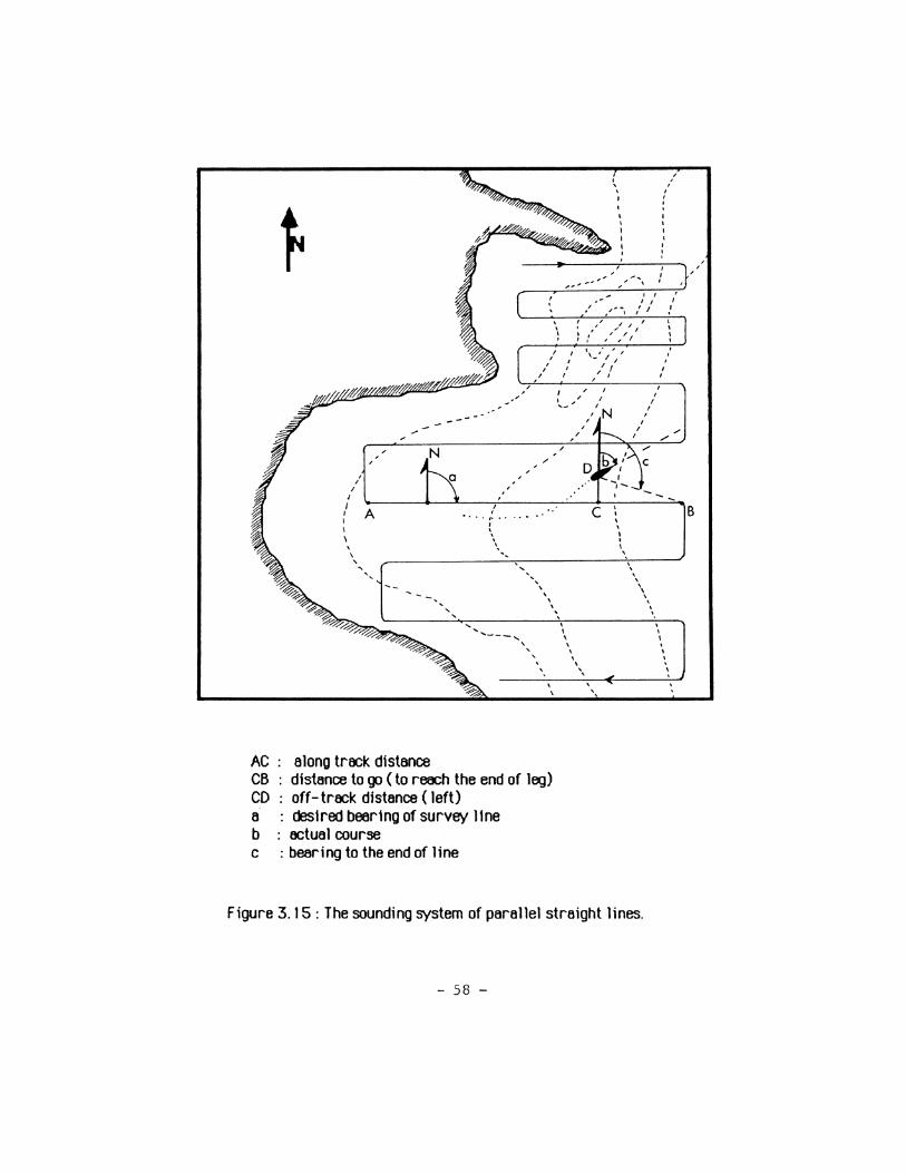
'
I,
' ' I I I 1 1 I I
' ,, ...... \
\ : ,'' .,/ I I I
:/ ,','1
N
I I a
I I I
A ' I I \
\ \
' ' '
' '
---
....
, , -·'
' ' ' ' I
' , . .. I
\ \ '•
.... ' '
I
' \
I
I I
I
/
' \ \
I
I ' I
,' '-' I ,' ' I I
I 11 I
I , I , I ,_" I
~N I ,
/ /
c I I \ \
I
' I \
.... '. ....
.... .... '--- .... ' ' ' ' \
AC along track. distance CB distance to go (to reach the end of leg) CD off-track. distance (left) a desired bearing of survey 11ne b : actual course c : bearing to the end of line
\ I \ \ \ \ \
\ \
\
\ \
\ \ \ \
Figure 3. 15: The sounding system of parallel straight lines.
- 58 -
I
' ' .
I
' '
' I I
I I
I I
' ' ' ' ' I .
\
' .
, ' I
I
'
\
,
B
I ,

The length of eoch leg and the line spocing should be variable (on-line). In this Wf!o/ close
water areas can be surveyed simultanously with the outer waters, and the density of soundings can
be increased with increasing seabed slopes (see also Figure 3.15).
The information that will feed the command DISPLAY consists of the following:
- distance to start of leg,
- distance to end of leg,
- distance off leg ( LIR indicator),
- desired bearing of line (corrected for m~tic declination),
- octual course (corrected for magnetic declination) and
- bearing to end of line (corrected for magnetic declination).
Generally it is easier for the coxswain to navigate along lines of constant bearing. In
oct1ition to the L/R indicator he compares the magnetic bearing to the desired bearing.
With regards to the general direction of survey lines, the tracks should preferably be run
at right angles with the isobath, as this will minimize the degree of uncertainty in charting of such
an isobath. The right angle intersection is clear but not always sufficient and not alWf!o/S easy to
carry out, as the octual directions of contours will only emerge during the survey. Another
restriction is that in many applications that require resurveys (e.g. monitor the movement of
sand waves) it is desirable to follow permanent survey lines. Also, when surveying waterwf!o/S, it
is desirable to run lines perpendicularly to the banlc:.s, because these lines will serve as bottom
profiles for volume computations.
Usually survey lines are specif1ed by a set of w~ points. A different approach useful for
channel surveying, is to specify as survey lines the lines that are normal or parallel to the central
line at equal distances. The table of w~ points contains:
- Wf!o/ point identification number,
- Northing and
- 59 -

-fasting.
The table of lines contains:
- llne ldent1f1cat1on number,
- Northing of start of line,
- East1ng of start of 11ne,
- Northing of end of line and
- East1ng of end of line.
SEAHATS provides navigation along parallel straight survey lines that are specified by a
set of WfJtl points. The following navigation information is displfJI{ed to the helmsman and launch
hydrographer:
- distance to start of leg,
-distance to end of leg,
-distance off leg ( L/R indicator with ripple plot),
-desired bearing of line (not corrected for magnetic declination) and
- bearing to end of line (not corrected for magnetic declination).
3.1.2 Investigation of seabed features
The general system of lines reveals a set of points, the shoels, which must be given special
attention since these points mf!t{ be hazards to navigation. This is called shoel examination . This
procedure is also used to locate obstructions reported to exist in a given area (searches). Usually
the least depth hes to be determined. The table of shoal points contains:
- shoel identification number,
- Northing of shoe I,
- Eesting of shoel and
- 60 -

- least oopth (if known).
Mainly there are three line systems to oolineate shoal areas or oo searches : parallel
straight lines, "circles" and "star" moOOs (Umbach ,1916,· Ingham, 1914), see Figure
3. 16 ( a,c and e). The system used depends on the location and shape of shoal. A basic requirement
is that the system lines should cut at right angles the contours of shoals. Each system should be
adjusted (on-line) to the current shoal configuration as illustrated in Figure 3.16 ( b,d,and f).
Parallel straight lines give an even coverage of shoal areas. Their use is OOffianOOd when
the soundings collected during shoal examination have to be plotted. In the "star" mode the
oonsity of soundings decreases as we go far from the shoal point. The "star" mode gives closest
coverage over the shoal and is best when the location Is known ~K:eurately ( 11nes cut contours at
right angles). The current position of the vessel must be included in the table of Wflo/ points. This
will help to refine the first leg of "star" mode. The "star" mode can waste both time and effort if
the location is vaguley known. Boudreau ( 1984 )suooests that the shoal coordinates should be
on-line re-established each time a shallower depth 1s measured.
For shoal examinations the following information is provided to the skipper:
for straight lines: -distance to start of leg
- distance to end of leg
- distance off leg ( l/R indicator)
- desired bearing of line (corrected for magnetic declination)
-actual course (corrected for magnetic declination)
- bearing to the end of line (corrected for magnetic declination)
for "circles" mode: - distance to start of leg
- distance to end of leg
- distance off leg ( l/R indicator)
- octual bearing
for "star" mode: - distance to start of leg
- 61 -

I I
--- --- .... .... --
~- ....... '--... --' -.....
\ I
I
/' /
\.
' \
'-
'
... , \ \ I
\. / I / ....__ / / ,. /
/ ~ /
~- / /
/ ..... _ ....
(a) parallel straight lines
(c) "circles" mode
(e) "star" mode
' ... ' ' '
I
,/
I \
'
/'
/
-----.... ---
,. I
' ....
.....
' '
---, ' ....
' --- ........ ........
--~ --- ... , \ ( \ I I
. ./ I I --- -- / I
/ ,. J~
'----'
(b) parallel straight lines unequally spaced
(d) modified circles to follow the coast line
I I \ \
' \ \
\ I
I I
'
(f) modified "star" mode to follow the coast line
Figure 3. 16 : Shoal examination patterns.
- 62 -
...... ,

- distance to end of leg
- distance off leg ( LIR indtcetor)
- desired bearing of line (corrected for magnetic declination)
- actual course (corrected for magnetic declination)
- bearing to the end of line (corrected for magnetic declination).
Appendix I gives the mathematicel models used to derive the above quantities.
SEAHATS provides shoal examination with straight parallel lines or the "circles" mode
or the "star" more. All of these sounding systems can be on-line adjusted to the current
configuration of the shoal area.
3.4.3 Cross and junction lines
The purpose of cross lines is to check the primary survey lines. The system of lines used
here is similar to the system used in primary lfnes. Details concerning their necessity.
orientation and density cen be found tn (Jmbach ( 1916).
Junction lines connect the soundings of two adjacent surveys. Junction lfnes may be of the
form of Figure 3.17a and 3.17b . In practice however, it is preferred to have overlaps between
surveys.
It is obvious that the functions Involved In hydrographic surveys (primary lines,
inestigetion of seabed features, cross and junction lines) can share two navigation sub-modules
named "circles" end "straight lines·. The functions are differentiated by the method that the
way points are specified (shoal points, start and end of legs).
- 63 -

leg 2
leg 1
(a) Step type junction lines (b) Arc type junction line
Figure 3. 17 : Types of junction lines.
leg 2 t leg 2
end of turn
start of turn leg 1
(a) w1thout ant1cipat1on (b) w1th ant1c1pat1on
Figure 3. 18 : W~ point navigation.
- 64 -
Channel navigation or steaming to the survey area requires that "route following· be
~to the navigation mooule. The route is specified by a set of Wflt{ points. But since it is not
necessary tor~ the points, or the navigation clearance around the Wflt{ points is not ~ate,
some means of anticipation must be 00'/ised. The next course must be triggered early enough to
avoid the vessel's overshooting (see Figure 3. 188). The user can preset the range of circle of
proximity where the automatic sequence of the next wflt{ point w111 occur and marie _the_ time the
ru!i:Er has to be put over. This range ( R) depends on the turning characteristics of the ship
(advance and transfer), that depend on the amount of rua:Er used and the angle (a) through which
the ship is to be turned. The vessel's speed has little effect (see Attwood et e/. , 1961).
Figure 3.19 incorporates the NAVIGATION module with the data acquisition system.
For SEAHATS, cross 11nes are run using the mode for primary survey lines. The system
also provides Wflt{ point navigation.
3.5 The ON-LINE MODIFICATION module
The ON-LINE MODIFICATION module is the lcey to the flexibility of SEAHATS (see Figure
3.19). While running survey lines there is often a need to view or mooify survey parameters and
continue to navigate without passing through the initialization procedure. A routine that will
interrupt the navigation function is needed. Here are some examples of where this routine is used:
- If the networlc of shore transponders gives high GDOP (Geometric Dilution Of Precision)
in the working area, the geometric configuration of control stations mflt{ be changed on-line to give
low GDOP (provided that there are enough transponders).
- 65 -
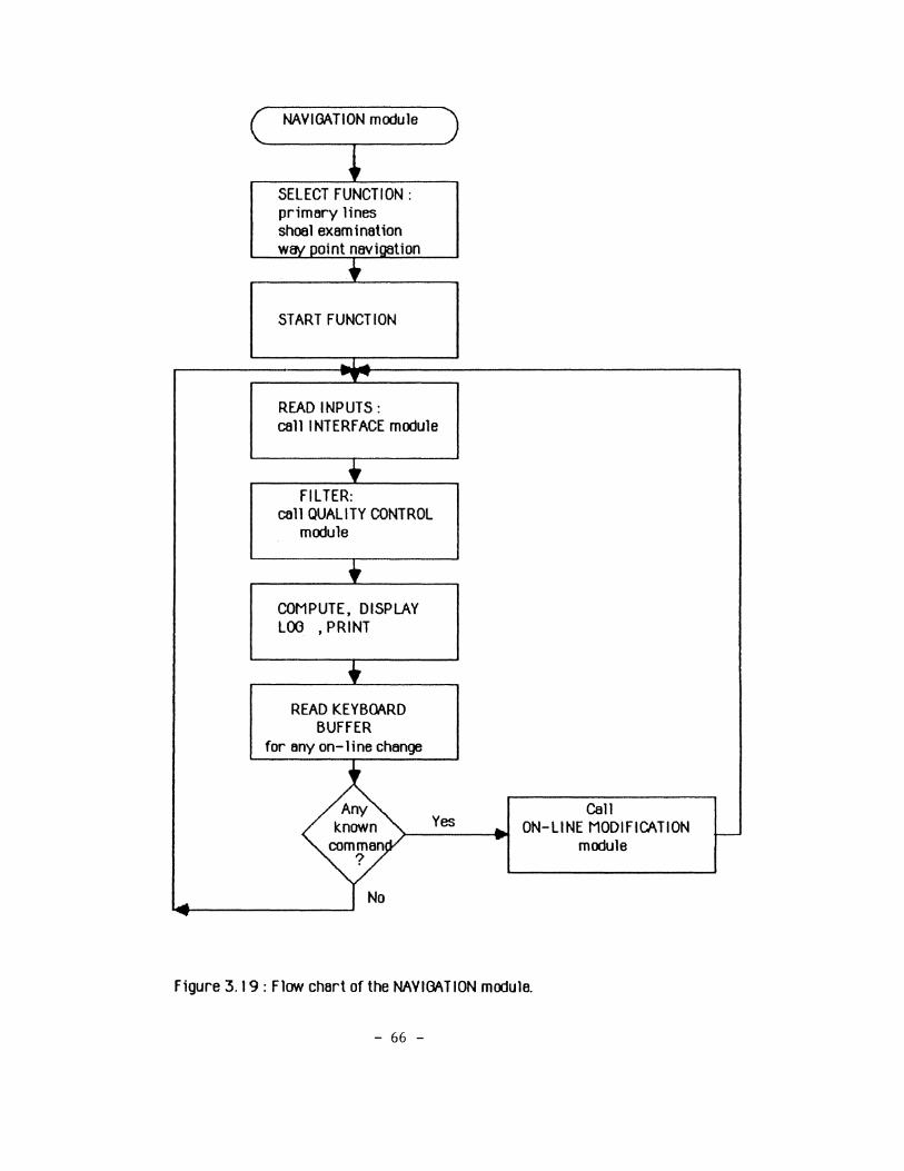
NAVIGATION module
~ SELECT FUNCTION : primary lines shoal examination way point navigation
+ START FUNCTION
-t--r""
READ INPUTS : call INTERFACE module
• FILTER: call QUALITY CONTROL
module
+ COMPUTE, DISPLAY LOO , PRINT
+ READ KEYBOARD
BUFFER for any on-line change
Any Call k.nown Yes .. ON-LINE MODIFICATION
r-com man module
?
No ... ....
figure 3. 19: Flow chart of the NAVIGATION module.
- 66 -

- If sea bottom slopes become steeper then more dense coverage is necessary. The
hydrographer would reduce spacing between survey lines to achieve the desired coverage.
After the change is made, control is passed to the navigation function. This interrupt,
when it occurs must not destroy computational integrity or disrupt any 1/0 operation. It has the
lowest priority among these procedures.
Since the C.P.U. of SEAHATS (Apple lie) cannot support multitasking, the navigation Is
suspended. The modification therefore should not tal<e more than 10 ~nds as otherwise the
skipper is left without steering information.
3.6 Description of current version of data acquisition system (SEAHATS)
The present data OCQUisition and navigation controller consists of the following
components :
1. Central Processor: Apple lie microcomputer.
2. Storage Device: 140 lcbytes floppy disks.
3. Positioning System: Motorola Mini Ranger System Ill (MRS Ill).
4. Interface Unit end Echosounder Digitizer: CADMI PSO 1.
5. Echosounder: Simrad Skipper 802 (with 50 I< Hz transducer).
The Mini Ranger System ( tfotorola, 19/JO) provides positioning Information to the
interface unit PS01 (Nickerson, 1983) via two parallel BCD connectors. At the same time the
echosounder digitizer (Harris, 1984) provides depth determination via another parallel
interface. The collected information with the associated time tag is sent to the Apple computer as
- 67 -

an input to the navigation ancllo;JJing functions. The interf~ module provires position and depth
correlation of the order of milliseconds. The structure of system is that of Figure 3.2.
Navigation functions include primary survey lines (parallel straight lines), shoal
examination ("circles" and "star· modes) and route navigation (up to 10 way points). Logging
functions include the logging of data 8nlrding to time or distance travelled. Navigation software is
written in UCSD Apple Pascal version 1.1 that runs under the Apple DOS environment. Software
is menu-driven with the exception of the ON-LINE MODIFICATION module which is partially
command driven in order to speed up the process of modification.
Position validation is performed using a gating technique. Depth verification is left for
post-processing for the following reasons:
(a) Depths reach the INTERFACE module at high rates ( 10 per second, see Harris
1984) but the CPU at lower rates ( 1 per second). It can be shown from equation ( 3.6) that if
we want to implement a gating technique and want to record sea bottom slopes of 450 steaming at
I 0 knots the estimated gate width is 10 metres. This value is not acceptable for shallow waters.
(b) A depth filtering algorithm will increase computational time, a critical factor for
microcomputers.
(c) Tests showed that the percentage of false echoes is small in the digitizer imp Iemen ted
here. False echoes are mainly produced when the echosounder 00es not track sea bottom. These
depths are usually very deep and can be eliminated by checking against a maximum depth.
As stated before, computation speed Is a limiting factor. In a real time application, such as
this, the skipper should have instantaneous display of the off-track distance. This fs not possible.
However, a certain amount of time can be tolerated without disastrous consequences. This amount
depends on the operator's experience and the vessel's speed and turning characteristics.
Experience shows that for small hydrographic boats, steaming at less than I o lmots this amount is
- 68 -
about 2-3 seconds. The current version updates the helmsman display every 3 seconds and
displays position history (ripple plot) for the past I 2 seconds.
There are basically two types of computer speed limitations (a) data transfer time
( -o. 70 sec at I 200 baud rate) and (b) data manipulation time ( -2.30sec). Data manipulation
time is the sum of execution time c- I .80 sec) and time for display updating (""'0.50 sec).
Errors detected in all phases of data ~uisltion can be classified into two types: warning
and fatal. The first type tells the hydro;Jrapher that inputs are unreliable but the execution of
navigation is not halted. Fatal errors indicate that the system is not performing well and
navigation stops. Warning errors are b8:t data sample format, b8:t disk 1/0 operation, etc ..
Incorrect inputs from the keyboard do not cause fatal errors. The inputs are read as character
strings, examined, converted to real or Integer numbers and then stored. 11c Cor thy ( 1983)
describes these error detection techniques.
The system RAM available for the Apple lie microcomputer is 64 kbytes. It is required to
store the Pascal Operating System, the executable code and data buffers. The 0/S occupies I 2
kbytes, leaving 52 kbytes available to the user. This memory is not enough to store the whole code
so, a portion of it resides on the disk. It is important that only non real time software resides on
a mess storage device es otherwise, cycling time will be increased by the time required to
perform a disk 1/0 operation (benchmarking results showed - 0.3 seconds). The mess storage
device for storing acquired data has a capacity of I 40 kbytes, which is enough for approximately
I 000 soundings.
- 69 -

4. OFF-LINE DATA PROCESSING
4.1 eeneral processing considerations
The introouction of computers to hydrographic surveys has chan~ the type and amount
of tasks of the hydrograph1c team as pointed out by 11ocdonold et ol. ( 1915). This processing
p~K:I<age is mainly <Edicated to the use of "Data Qlllector" the third level of the hydrographic
team, the others being the "Hydrographer in Charge" and the "Data Processor".
The trooitional role of the "Data Q)Jiector" or launch hydrographer is to conn the survey
vessel along pre-ootermined tracks, collect position, oopth, time and any other relevant
information useful for post-processing. The hydrographer in the field wants to know how his
survey is progressing in a very short perioct of time. Therefore, during or just after data
collection, he portrays the data to ioontify shoal areas or gaps in his surveys. This implies that a
certain amount of data processing has to be carried out in the field (e.g. reduction to the datum of
reference, removal of blunoors) before data is fed to the "Data Processor" for final presentation.
This amount of data processing, called "field data processing", is oone manually. The tloo
is interpolated from tire tables and soundings are plotted manually. This requires an fOiitiona\ 3
- 70 -

to 4 hours of work for each day of data collection. The software package discussed here tries to
minimize this extra work.
It must be emphasized that the computer resources necessary to speed up this process
must be available any time during the survey work. The computer facilities of the hydr<YJraphic
office or the "mother ship" are not suitable. The best Wfl./ to further process the data off-line is
to use the acquisition computer &ystem. The finar proouct will be rough field sheets accompanied
with the associated corrections.
This processing package ooes not replace the task of the "Data Processor" but rather helps
it. For example, if the purpose of survey is chart proouction, the ·Data Processor" is responsible
for merging data from different sources, contouring and performing quality control on the data.
These tasks require stronger computer capabilities than the acquisition computer &ystem can
provide and a great amount of juO]ement and knowled;Je. For the sake of completeness, however,
methods for off-line quality control of data and Wf1./S for final presentation are discussed.
Data ,processing consists of five elements :
(a) EDITING,
(b) REDUCTION and CORRECTION,
(c) SMOOTHING,
(d) SELECTION and
(e) PRESENTATION.
We cannot draw distinct boundaries between the amount of correction, reduction,
smoothing, selection and data presentation that is oone on-line and off-line. For example,
correction for roll, pitch and heave effects can be oone either on-line (by integrating to the
&yStem roll, pitch, heave sensors) or off-line (by merging separately collected heave and depth
data).
- 71 -

The field data processing is an iterative process. It is repeated until the launch
hydrographer ( with the assistance of hydrographer- in-charge ) has strong evidence to choose to:
-resurvey the whole area or part of it,
-fill survey gaps,
-examine shoal areas or
-provide the collected data to the "Data Processor".
1.2 Interactive edUtng of hydrographic data
The objectives of an interactive editor for hydrography are:
(a). To correct identified errors in the location and value of a sounding.
(b). To delete soundings collected during a shoal examination and used to reveal the
shallowest depth.
(c). To fill gaps between soundings (merge soundings from different sources).
(d). To identify the shallowest point in a given area.
In order to meet these objectives the editor must have the ability to acti, delete, move,
chanae, suppress, unsuppress or search soundings or survey lines. To oo this, the operator
must have the capability to identify where the soundings or lines come from and treate them as
Inputs.
The changes in soundings must be registered on the survey data files. In order to
implement the features of the editor, it is necessary to design a data base successfully. Yerme
( 1984) describes the editor and ttelone ( 1984) describes the data base used in the Can~ian
Hydrographic Service. The design of such an editor and data base is beyond the scope of this·
- 72 -

research. We will restrict ourselves in the implementation of simple editor commands like lrtl,
delete and change.
A major reason for using a commercially available system like the Apple lie
microcomputer and not a specialized system lil<e the HY-NAV, is thet editor features are
provided. SEAHATS makes use of the P8SC81 Operating System editor to lrt!, delete or change
soundings.
<t.3 Smoothing, correction and reduction or hydrographic data
The next phase of processing the recorded data (positioning and bathymetric) is to
smooth them by applying our knowled]e about the behaviour of depths and position. Then, the
observed soundings are corrected from departures from true depths and are reduced to the
reference datum. These corrections inchl:E (Thomson eta/., 1981,· Umbach, 19 76):
(a) Transducer correction (static draft, settlement and squat).
(b) Correction of different sound velocities in the water column.
(c) Reduction to datums of reference.
(d) Ro 11 , Pitch, Heave corrections.
Figure 4. 1 illustrates corrections (a), (b) and reduction (c). Usually these corrections
are applied off-line. Correction (d) is shown in Figure 4.6 and it is an underway correction.
Static draft 1s the depth of transducer when the vessel ls at rest. Settlement ls the
difference in depths of transducer when at rest and underway. Squat is the change in vessel's trim,
while underway, that changes the verticality of the transducer.
- 73 -

-4D
vessel at rest
water surface vessel's keel
underway
sea bottom ~---P------~------~------------~----~~~~--------.,
(a) transducer correction
c: 0 ...... - water surface g "0 olD L
'i) reference datum > olD "0
olD L > C) L .c. - C) .c.
~ B - -0.. 0.. 41) ., "0 "0 - c; L
~ :::J -u u ., sea bottom
(b) datum reduct ion and sound velocity correct ion
Figure 4. 1 :Corrections and reductions to observed soundings.
- 74 -
The two main factors that cause an increase in squat, are increasing speed and decreasing
unrer keel clearance. Decreasing unrer keel clearance is important only when the ratio of
repth/static draft is less than 2.5 (Bowditch, 1911 ). For launch hydr~raphy with static
draft of the or!Er of 1 metre, the effect is negligible. The increase in speed results in a Mdown by
stern" squat which 1s also neg11g1ble for speeds less than 10 knots. Transducer correction 1s
therefore constant and equals the static draft.
With SEAHATS processing software, !Epths are corrected from static draft and different
sound velocity in the water column. Soundings are reduced to the datum of reference. Roll, pitch
and heave corrections are not provided. The effect of ignoring these corrections (roll, pitch and
heave) is investigated in section 4.3.5.
1.3. 1 Smoothing of positioning data
In section 3.5 it is mentioned that in SEAHATS a gating technique is used to block out
wild ranges. Now we will further smooth the ranges to Mini Ranger transponders using a
s-imple linear morel with driving noise. An off-line filter is reveloped that uses fixes before the
fix unoor consi!Eration. The factors which prevent on-line implemenatation were discussed in
section 3.3.3.
The dynamic miXEl that describes the behaviour of each range to control station for short
time perfros 1s :
R1c = Rk-1 + Vk-1 t + 112 ak-1 t2
V1c ""V1c-1 ... Btc-1t
where:
- 75 -
( 4.1)
(4.2)
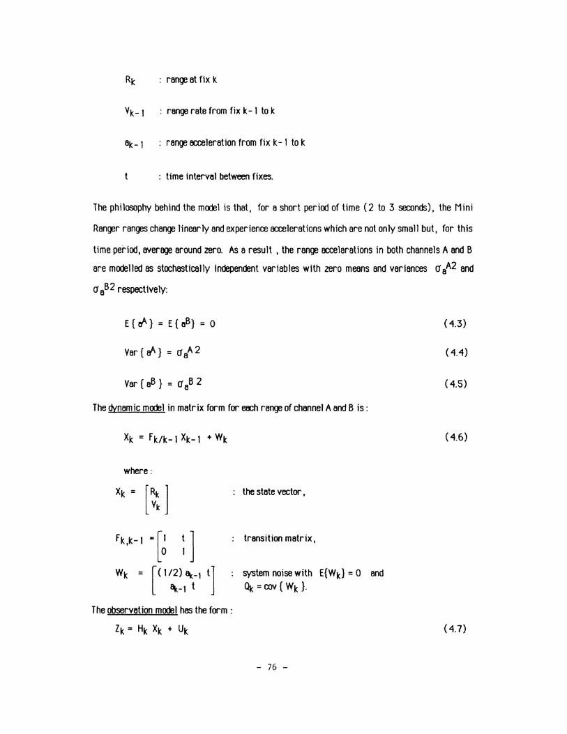
RJ< : range at flx k
Vk- 1 : range rate from fix k-1 to k
BJ<-1 : range acceleration from fix k-1 to k
t : time interval between fixes.
The philosophy behind the mOOE!l is that, for a short period of time ( 2 to 3 seconds), the Mini
Ranger ranges change linearly and experience accelerations which are not only small but, for this
time period, average around zero. As a result , the range accelerations in both channels A and B
are modelled as stochastically independent variables with zero means and variances 0' 8A2 and
0' aB2 respectively:
var { aB } = 0' 8B 2
The Wnamic model in matrix form for ~h range of channel A and B is:
where:
Fk k-1 ' : ]
W~c = [( 1/2) t\-1 tl t\-1 t
The observation model has the form:
Ztc = Hk Xk + Uk
the state vector ,
transition matrix,
system noise with E{WJ<} = 0 and ~ = cov { WJ< }.
- 76 -
( 4.3)
( 4.4)
( 4.5)
( 4.6)
( 4.7)

where: H1c = [ 1 0] the matrix that relates the observations with the state vector, U1c the
observation noise with E {U~c} = 0 and P~c=Var{U•:l =O'R2 and O'R the range variance. The
derivation of normal equations can be found in tJrant ( 19 76).
The presence of driving noise W1c allows the hydrographer to tune the filter in the actual
survey conditions. This is because the main function of the driving noise is an indicator of the
accurfLY of dynamic mroel. This implies that , in rough sea, where rolling and pitching of the
vessel's antenna intrrouces high range accelerations and the positioning system is stable, range
observations are stronger than the estimates derived from dead reckoning. This lcnowleO;Je is
reflected in the selection of the filter gain factor.
As mentioned in Janes ( 1983) , the gain of the filter is fixed for any constant ratio
O~c/P~c ( 01c is the model noise covariance and P~c is the observation noise covariance) , regardless
of their sizes. In the present filter we have Qlc = E { WJc WJc T } which results in :
We also have:
(l/2)t3J
t2 (4.8)
( 4.9)
The gain Is equally sensitive to Ole and PJc, which means that the ratio k=OJciPJc uniquely def1nes
the behaviour of the fi1ter.
figure 4.2, curve (a) depicts an actual range rate time series from channel A of the Mini
Ranger System, obtained by differencing consecutive measured ranges. The survey boat was
running parallel straight lines at Campobello Island. Curves (b), (c) and (d) are estimates of the
range rate (VA) with tuning factors lc = 0.0 I , 0. I and I respectively. For large measurement
noise and small system noise, the gain of the filter is small and only small adjustments will be
- 77 -

c:.-;:J
.~ 4
a
n 3
9 e 2
r 1
a
t 0
e
-....! I -1
co i
n --2
m --3
/
s --4
-·5
~·· 11 lltl•l
~~~ llr\ ~ 'I ' ~I j, '
1 2. 45 12. 5 12. 55 12. 6 12. 65 12. 7
time in hours
Ftoure 4.2: Estimation of Mini RenQer renoe rete ttme series 'w'1th Kelmen f11tertno for various gein factors.
! ~,j i j l
12. 75
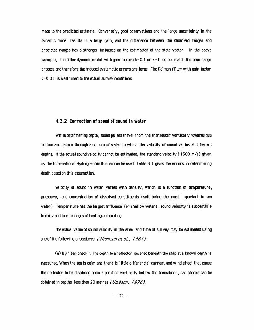
mtO! to the predicted estimate. Conversely, ~ observations and the large uncertainty in the
dynamic mll:El results in a large gain, and the difference between the observed ranges and
predicted ranges has a stronger influence on the estimation of the state vector. In the above
example, the filter dynamic mll:El with gain foctors lc=O.I or lc= I do not match the true range
process and therefore the Induced systematic errors are large. The Kalman filter with gain foctor
lc=O.O I is well tuned to the octual survey conditions.
4.3.2 Correction of speed of sound in water
While determining depth, sound pulses travel from the transducer vertically towards sea
bottom and return through a column of water in which the velocity of sound varies at different
depths. If the octual sound velocity cannot be estimated, the standard velocity ( 1500 m/s) given
by the International Hydrographic Bureau can be used. Table 3.1 gives the errors in determining
depth based on this BSSumption.
Velocity of sound in water varies with density, which is a function of temperature,
pressure, and concentration of dissolved constituents (salt being the most important in sea
water). Temperature has the largest influence. For shallow waters, sound velocity is succeptible
to daily and local changes of heating and cooling.
The octual value of sound velocity In the area and time of survey may be estimated using
one of the following procedures (Thomson eta/., 1981):
(a) By " bar checlc ". The depth to a reflector lowered beneath the ship at a lcnown depth is
measured. When the sea is calm and there is little differential current and wind effect that cause
the reflector to be disploced from a position vertically bellow the transducer, bar checlcs can be
obtained in depths less than 20 metres ( l/mbach, 19 76).
- 79 -

(b) By directly measuring sound velocity as a function of depth using an eccurately
calibrated velocimeter.
(c) By measuring temperature, salinity and pressure (depth) along the water column and
using Wilson's approximate formula.
(d) By referring to tables of sound velocity corrections for the same area at a sim11ar
time of the year.
Matthews' tables ( 11at thews, 1939) are the reference tables for the last case. ~s
are divided into oceanographically similar areas and sounder corrections are tabulated for these
areas. Their use is not recommended for shallow waters because of their very general nature.
Such procedures are recommended for ships engaged in hydrographic surveys on the deeper parts
of continental shelf. Matthews' velocities oo not include variation with pressure and it was found
that the surface estimates are 3-4 m/s too low.
Wllson 1960 (Wilson, 1960) Includes variation with pressure In the determination
of sound velocity. The dependence of sound velocity on temperature, salinity and pressure within
I 000 metres of the surface is found approximately :
c = 1449.2 + 4.6 T - o.ossT2 + o.ooo29T 3 +
( 1.34- O.OlOT)(S- 35) + 1.58 to-6 Pa
where:
C : sound velocity ( m/s)
T : temperlrture {CO)
S : salinity ( ppt)
P a: gauge pressure due to water column ( N/m2).
( 4.1 0)
If we ignore compressibility Pa = Pa!JZ (p11 : water density) and using Pa=< 1+Slo-3)to3
Kgr /m3 , g=9.8mtsec2, S=35ppt and z=depth the variation due to pressure is 0.0 16z.
- 80 -
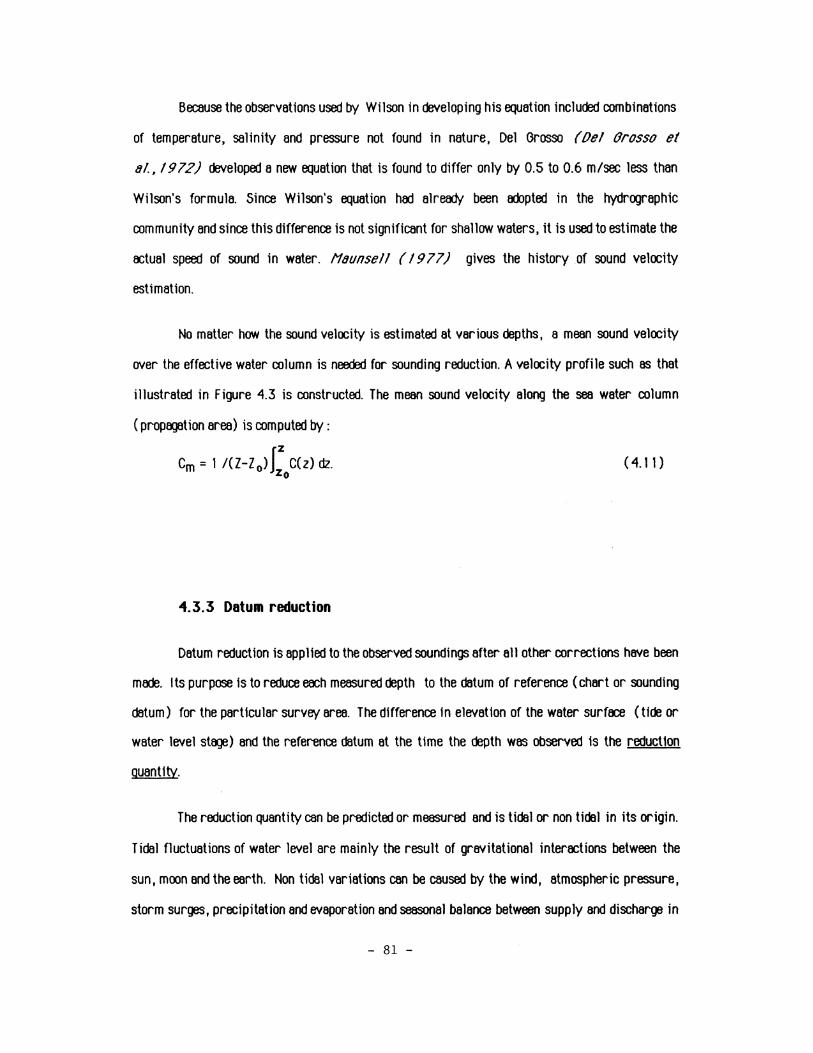
Because the observations used by Wilson in !Eve loping his equation included combinations
of temperature, salinity and pressure not found in nature, Del Grosso (Del Orosso el
of., 1912) ooveloped a new equation that is found to differ only by 0.5 to 0.6 m/sec less than
Wilson's formula. Since Wilson's equation had already been adopted in the hydrographic
community and since this difference Is not significant for shallow waters, 1t is used to estimate the
actual speed of sound in water. ttounsell ( 1911) gives the history of sound velocity
estimation.
No matter how the sound velocity is estimated at various depths, a mean sound velocity
over the effective water column is needed for sounding reduction. A velocity profile such as that
illustrated in Figure 4.3 is constructed. The mean sound velocity along the sea water column
(propagation area) is computed by :
Cm = 1 /(Z-Z 0 ) r C(z) dz. Zo
( 4.11)
4.3.3 Datum reduction
Datum reduction is applied to the observed soundings after all other corrections have been
made. Its purpose is to reduce each measured depth to the datum of reference (chart or sounding
datum) for the particular survey area. The difference In elevation of the water surface (tide or
water level st~) and the reference datum at the time the depth was observed Is the reduction
guantltv.
The reduction quantity can be predicted or measured and is tidal or non tidal in its origin.
Tidal fluctuations of water level are mainly the result of gravitational interactions between the
sun, moon and the earth. Non tidal variations can be caused by the wind, atmospheric pressure,
storm surges, precipitation and evaporation and seasonal balance between supply and discharge in
- 81 -

sound velocity sea surface ..
,,
Figure 4.3: Sound velocity profile in the area of survey.
FREDERICTON. N.B. 1969 ·1979
Fut Ju. ftb. Mar. A,r~ Mo June July A.v. Sept. Oct . ..... Doc. Metna
"*• Je•w ftv. Mor Avril Mai Juin Juil. Aout Sept Oct. ... .. Dk Mttrn
20·0 6·0
16·0 - 4-6 f--
12·[) /\ 3-6
I --r-
8·0 H v ~
- f--- - ;r-- - r--
4-0 1·2 - - - "--- .~ ............... ~t-;+~· - -.. 0 •. . --:.-: . 0 ..
- 4·0 '"·1 'TT::i .~.1::.1· ·~· . -1·1
r
' I I I
Figure 4.4: Se8SOnal variation of water level in Saint John river.
- 82 -
rivers. The tide usually oominates the spectrum of variations of water level fluctuations but in
some cases, as in rivers, the tidal range is very small compared to larger variations in water
level due to the seasonal disturbances (see Figure 4. 4 for Saint John river In Canooa).
Prediction of the astronomical tides for inshore waters is based on the description of the
tide by means of constants which can be determined by harmonic analysis applied to an observed
timeseriesoftide heights in deeper waters (Oronkers, /964). In hydrographic surveys in
shallow sea waters and rivers, the description of the tide using only the astronomical constants is
in008quate and "shallow water constituents• must be considered as well ( Oronkers, 196 4).
The prediction model is complex and not pr8:tical. Complexity is increased when models for wind
set up or atmospheric pressure effects are lrl:ted.
Prediction models are used for off shore surveys where it is difficult to set up a tide
monitoring station, and the tide motion is well predicted by cotidal charts. For automatic
reduction of soundings that use predicted models see Okenwa ( 1918).
It is therefore required that a tide gauge be set up in the vicinity of survey area, and the
rise and fall of tides observed while soundings are taken. Often the onsite tidal data differs from
the data of the monitoring station in the range and time of arrival of a particular phase. In that
case, the survey site is surrounded by a number of tide gauges and appropriate interpolations can
provide 8:CUrate tide height estimates. For more details on the selection of these sites see
Umbach ( 1916).
Mainly there are three methods of interpolating tidal data in the tide record, depending
upon the 8:Curacy requirements and the sampling interval (Umbach, 1916). These are: (a)
linear interpolation between readings, (b) scaling of values In a plotted curve, and (c)
construct ion of a reduction table.
A version of the second method requires the observation of only two successive high and
low values. Intermediate values are computed by approximating the tidal curve with a sine curve.
- 83 -

If ( T 1 , H 1 ) and ( T 2 , H2) are two successive high and low points in the tida 1 record the tide ( H)
at time (T) is:
( 4.12)
The application of the method is straight forward when the charocter of the tide is diurnal
or semi-diurnal. When the tide is of a mixed type, it is sometimes difficult to distinguish
between successive low and high values. Figure 4.5 represents an octual tide record and its
approximation at Campobello Island N.B., where the tide is semi-diurnal. The octual tide record
has been constructed with re81ings every 5 minutes (the height spikes are recording errors). It
can be seen that the sine curve agrees with the tide record within I 0 em. SEAHATS processing
software includes this technique for tide reduction.
"'1.3."'1 Establishment of the sounding datum
There is often a need to refer the local sounding datum to the chart datum. If the chart
datum cannot be determined from existing benchmarks close to the survey site, it can be obtained
by water level transfer from a near site where a chart datum exists. Thus, processing software
should include a utility for water level transfer.
Water transfer implies simultaneous observations of short perioo ( 3 to 4 days) of the
water level at the site of the survey and at one or more reference stations in the vicinity of the
aree (e.g. 50 lcm ). The method used for transferring water level depends on the main generating
force of water level fluctuations (tide, wind, seasonal balance between supply and discharge in
rivers, atmospheric pressure etc.). Forrester ( 1983) gives a description of these forces.
- 84 -

6
5. 5
t 5 1 d 4. 5
"'4
1 3. 5
n 3
m 2. 5
"' t 2
,... 1. 5
"' 9 1
• 5
0
--acluoltide
g 10 11 12 13 14 15 16 17 19
timg in hours
Figure 4.5: Semi-diurnal tide at Campobello Island and its sine curve approximation.
Table 4.1 :Accuracy ( RMS errors) of ootermination of water level using a 3-day period of observations (from Aboh 1983).
area of area of area affected SOUNDING changing changing by river METHOD DATUM range character and estuarine
effects Range
MLW Ratio 40cm 20cm 4cm
Height MLW 37 em 15cm 3cm Differena
Ext. Water Elevation MLW 50 em 47cm 14cm
- 85 -

In cases where tide is the main contributor to variations in water level, three methods are
chiefly used for transferring water levels and establishing a sounding datum. Aboh ( 1983)
describes these methods. These are : Ranoe Ratio, Height Difference, and Extraoolated Water
Elevation methods. Selection of the best method for a particular area and time depends on how
closely the assumptions on which the methods are base are met. The Range Ratio method has been
used for years. Forrester ( 1983) says that this method perfor _ _rns well when the tide is
semi-diurnal or mixed semi-diurnal (as in the Bay of Fun~).
Aboh ( 1983) also compares the three methods in areas of different tide character,
different range, and areas that are affected by river and estuarine effects. The Height Difference
methoo performs well in all these areas with an accuracy in deriving Mean High Water (MHW)
level of 27 em and Mean Low Water level of 37 em RMS (see Table 4.1 ). Therefore, the SEAHATS
software processing pacKage includes the Height Difference and Range Ratio methods to estimate
ML W which will be the sounding datum closest to the chart datum.
Water level transfer in non-tidal waters ( as in lakes and rivers ) should not be carried
out when wind set up or seiche ~~::tivity is suspected. Without these ~~::tivities, the mean surfll::e in
lakes is the seme everywhere and in rivers is only affected by surfll::e slope. Forrester
( 1983) gives the procedures for performing level transfers in these cases.
4.3.5 Roll, pitch, heave corrections
In this section we w1111dentlfy the need to correct the observed depths and estimated ship's
position from ship motions caused by the wave ~~::tion. The hydrographic vessel, underway, is
subject to six motions that can be attributed to the motion of waves. These are three displll::ements
(heave, surge and sway) and three oscillations about the principal axes of the ship (roll, pitch and
- 86 -

yaw, see also Figure 4.6). Only roll, pitch and heave affect the observed oopths. Roll, pitch and
heave correct1ons are d)tnamlc, periodic corrections and are usually applied unoorway.
Figure 4.6 illustrates how a vessel's roll and pitch affect the verticality of the transducer
and thus the measured depth. Heave is the vertical displacement of the transducer from mean water
surface due to sea conditions. Estimation of these corrections requires sensing of angles a (pitch),
b (roll) and vertical acceleration (c). The corrected depth is:
Dtrue = Dooserved + C roll,pitch + Cheave
C roll,pitch = Dobserved { ( 1 /(I ( tan2a + tan2b + 1 ) )- 1 }
Cheave= - IJ c dt ,6-1:
( 4.13)
( 4.14)
( 4.15)
The pitch angle of vessels is normally in the range of 5 to 1 0 degrees and much smaller
than the roll angle, which can be up to 25 degrees. Figure 4. 7 gives the error due to roll and
pitch of a vessel for oopths of 100 metres deep. In shallow waters and in good sea conditions, the
errors due to roll and pitch are negligible. More important is the heave effect which can be 2
metres at a period of 5-10 seconds (Hopkins, 1980). Rolland pitch always give measured
oopths that are deeper than true depths.
Heave is ootermined by measuring vertical acceleration and integrat1ng twice to obtain
vertical dlsp lacement. The heave sensor Is resigned for a specific bandwidth of heave periods (e.g.
1 to 30 seconds). Outsloo this frequency envelope, the heave estimates are false. The wloor the
bandwidth the better the sensor. But such a sensor also senses lower frequency components caused,
for example, by horizontal accelerations due to maneuvering. For example, a goo change in the
ship's course at a speed of 8 knots, introduces a false heave output or 30 em. This output is
proportional to the square of the ship's speed (Hopkins, I 980). These frequencies have to be
blocked out. A high pass filter is needed which requires 1-2 minutes processing time. Two
methods are proposed by Hopkins (I 980) to compensate for heave:
- 87 -

antenna (Xa.Ya)
t. heave
transducer (Xt,Yt)
bow
Figure 4.6: Ship motion due to wave action and its effect on depth detemination and position of the antenna of positioning system.
- 88 -
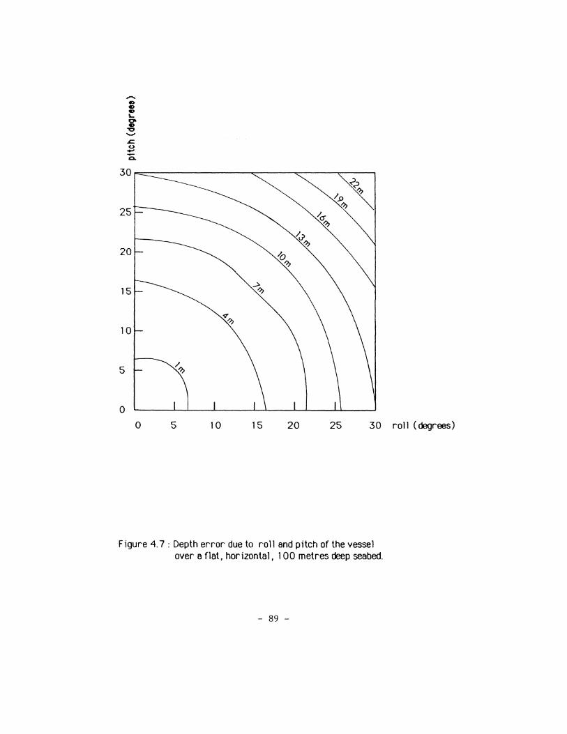
s::. 0 -c.
0 5 10 15 20 25 30 roll (degrees)
Figure 4.7: Depth error due to rolland pitch of the vessel over a flat, horizontal, 100 metres deep seabed.
- 89 -

(a) to approximate heave in real time with reduced bandwidth or
(b) to estimate error free heave with wider bandwidth but delayed by more than
I minute.
For the present real time application it is suooested that methOO (a) be ampted. This
requires surveying within the frequency range of the heave sensor and avoiding depth observations
while maneuvering.
Hopkins ( /980) also gives the equation needed to calculate the so-called translation
correction. This correction, which will not be further Investigated here, is needed when the heave
sensor cannot be installed in the same location as the sonar transducer and therefore experiences
different fa:eleratlons.
We can manually smooth the effect of rol I, pitch and heave on the echogram and therefore
we do not need any special hardware. But if the bottom has irregularities of similar magnitude to
the wave length of heave, manual smoothing will result in an incorrect picture of the sea bottom.
Due to the roll and pitch of the vessel, the coordinates of the antenna of the positioning
system (X8 ,Y8 ) do not coincide with the coordinates of echosounder transducer (X8 ,Y8 ) (see
Figure 4.6). For small hydrographic launches with a I 0 metres mast, and roll and pitch angles
less than 5 degrees, the offset In coordinates is in the order of 1 metre. For larger values of roll
and pitch it is necessary to use roll and pitch sensors.
- 90 -

4.4 Selection and presentation of results
4.4. 1 Selection of soundings
Soundings from their "generation" to their presentation on the final field sheet go
through three stages: fflterlng, selection for storing and selection for presentation that alter
their quality and quantity,
Filtering occepts soundings on 8 time base as discussed in chapter 3. Selection procedures
select soundings on 8 time base, .or on a distance base, or on 8 distance and depth difference base.
The selection method that will be used depends on the application. Selection on a time base
Is simple to implement but variations In the vessel's speed result in gaps or overplots of
soundings. For example, runnirg lines normal to the shore lines accumulates soundings near the
shore line. Logging data on a fixed along traclc distance Interval portrays sea bottom evenly
independent of variations in vessel's speed. Both the above methods may fall to reveal critical
depths. To overcome this we may choose the shallowest (for navigation purposes), the average
(for dredging operations}, or the deepest depth over the travelled distance or time. Averaging
over time has the advantage that, if the time interval over which we average equals the period of
heave, the depths are compensated for heave.
A more sophisticated 8pprooch is to log data based on two criteria: the maximum distance
between two adjacent soundings and their minimum depth difference. This technique is widely used
in CHS ( 11acdonald, 1984). The above two parameters are variable and depend on the sea state,
bottom roughness and the intended use of the data
In tniitlon to the above automatic depth selection methods, in some app11cations it is useful
to select depths manually. Selection of depths at the start or end of survey legs or at specific
points along the traclc must be also under the hydrographer's control.
- 91 -

The main purpose of selection procedures is to accurately depict sea bottom topography. In
aalition, when the survey proouct is a navigation chart, selection for presentation is responsible
for selecting portable depths. The procedure, taking into consideration survey scale and size of
depth digits, must show as many depths as possible without overplotting, and if some depths can
not be plotted, It ensures that the shallowest is retained.
In SEAHATS, soundings are selected in real time. The user has the option to select
soundings on a time base or on a distance base. All the !DlUired soundings are plotted.
1.1.2 Shoal detection
In section 3.4.2 we dealt with procedures to determine the least depth in a shoal area. In
this section we will show what to look for in the general system of lines that indicates these areas.
The first step is to determine how closely we have surveyed the area, or in other words, to
find the probabllity of finding an underwater obstacle. If this is high, almost nothing lfes
undetected between the lines and there is no need to proceed further. Stenborg ( 1984)
develops a probability model that is based entirely on the geometry of the survey (see also Figure
4.8):
m = m0
m = 1 when m0 <= I and
when m0 > 1
where:
m :probability of finding an underwater obstacle, m0 = ( d + 2( D-e)tan( b/2)) IS, S :theoretical spacing between survey lines, D : depth of water, e : echosounder draft, b : echosounder beamwidth and d : diameter of a circular underwater feature.
- 92 -
( 4. 16)

F =2( 0-e)tan( b/2) : echosounder footprint diameter d: diameter of a circular undrerweter obstacle S: spacing between survey lines
d+F ffio=----
s
Figure 4.8 Geometric probability of finding en underwater obstacle.
- 93 -
This mcml BSSumes that the offset of the survey line from lts theoretical position is
negligible. Of course, this mcml can be applied before surveying to estimate an optimum sounding
Interval.
If the estimated probability is two low, IJmbach ( 19 76) suooests that we scan the
sounding profiles for protrusions that indicate shoals, or examine aerial photographs, or look for
kelp indications and reports of dangers from reliable sources.
ttonahan ( 19 75)suooests a morphometric approach to the problem of shoal detection.
He claims that, for specific morphologic types (e.g. sea mountains), a relationship can be
established between the number of profile protrusions in the survey aree and the number of these
protrusions that belong to the morphologic type. If this relationship is known the morphologic
type can be extracted by examining the distribution of protrusions in the general system of lines.
Field shoal examination starts from this point.
It must be emphasized that the effectiveness of this method depends on how well one has
understood its limitations. For example, the method is unable to detect a wrecl<, if the wreck lies
entirely between sounding lines, although its morphologic type may be known.
1.1.3 Presentation of results
The collected data is dedicated to the charting of navigational waters or to the needs of
engineering constructions in waterways and harbours. These applications have different
requirements associated with the depths. To fulfill these requirements, information is
manipulated in different ways.
- 94 -

Since navigation safety is a prime requirement when prOOllcing charts, the presentation
mooule should portray all extremes, the ooepest and especially the peaks. In addition,
hydrographic data has a set of characteristics that affect the choice of an appropriate technique.
Such characteristics include the: clustering of data in co-linear fashion (ship's tractcs) and the
existence of discontinuities (cliffs, pinnacles). Robson ( 1914) describes the nature of
hydrographic data.
Usually, contouring techniques are used to portray the data. These are grickled or non
gridded. Non-gridded techniques honor the original data more than gridded and therefore preserve
dangerous peak values. But, the uncertainty in the formation of triangles does not justify its use
for hydrography (Sal/away, 1981 ). Gridded methods are suitable for navigation purposes
only if the interpolation method used is shoal biased. This means that the shallower points
contribute more in the determination of depths in the grid nodes.
The inabllity of the present contouring techniques (used for hydrographic purposes) to
Incorporate any surface trends ts pointed out by many authors. C/oet ( 1984) clatms that
when the seabed has strongly linearized features, such as sandwaves, the contouring
representation may give misleading results. These features, for the sake of legtb1ltty, are
sacrified. He also suooests an intermediate stage in processing the data involving a pseudo 30 plot
of the data. The survey lines run are plotted, after scale and tidal datum reduction, by stacking
them sequentially. The bathymetric surface developed in this way may have some irregularities
due to the fact that the survey lines are not perfectly run. However, these can be corrected by
Interpolating from adjacent prof11es. This representation is also an effective shoal detection
technique.
If the post-processing module is primarily geared towards dredging surveys, volume
computations must be included. Bathymetric chart representation displays the overall picture of
the seabed, but for dredge volume computations, the inherent approximation errors from these
methods cause considerable inaccuracies in volume computations. In practice, volume
- 95 -

computations are performed using profiles. It is preferable to use as profile lines those generated
in the acquisition process.
4.4.4 Data basa management
In this section we assume that the gathered data is used for charting coastal waters. The
data should be included in a Hydro;)raphic Data Base. We wm identify what quantities the system
has to provide to the Data Base suooested by tfolone (I 984).
According to Malone the Hydro;Jraphic Data Base consists of five data bases:
(a) Reference Data Base,
(b) Raw Data Base,
(c) Cleaned Data Base,
(d) Field Sheet Data Base and
(e) Chart Data Base.
The Reference Data Base controls information now among the other Data Bases. It
requires the chart number, establishment, scale, year of survey, location and status of survey.
The Raw Data Base has as entity the "sounding" and as attributes:
- identifier (establishment, vessel, day, time ,location)
- control station file
- Wf!Y points file
- tidal data file
- parameter file (sound velocity, line sps:ing,filtering parameters etc.).
- 96 -

The Clean Data Base requires the corrected sounding file with the list of corrections
applied:
- Identifier (establishment, vessel, day, time, location)
- corrected and reduced sounding file
- tide corrections, sound velocity corrections, datum transformations
- number of field sheet the sounding lies ln.
The corrected sounding file (X,Y and Depth) of the Clean Data Base, without the listing of
applied corrections, forms the data required by the fourth data base: the Field Sheet Data Base.
The Chart Data Base requires the soundings that have been chosen from the Field Sheet
Data Base to represent bottom topography through the "sounding selection" procedure.
4.5 Description of SEAHATS data processing package
The processing pr£kage uses the same C.P.U. as the acquisition system. An Epson printer
and the Hewlett Pf£kard HP 7470A plotter are 6ijed to the system.
Raw data consists of the following files. Sounding file: contains, in digital form, date and
time of survey, leg and fix number, code numbers of control stations, ranges to control stations
and range signal strengths (optional), position, depth and covariance matrix of position. At
present the covariance matrix does not convey any statistical information since there are no
redundant observations. Control file : contains the coordinates of reference stations for the
particular sounding file. Ww file : is the set of wery points used to form the survey lines and the
shoal points that need investigation. Tide file: is the table of observed tide heights consisting of
location, year, day, time and tide height. Sound velocity file': is also a table of either sound
velocity observations and depths, or observations of salinity, temperature and depth.
- 97 -

The editing system is based on the ability to point at material currently displayed and
treat it as an input. Apple lie supports (X,Y) display cepture devices (such as the mouse, joy
sticks and light pen) but these devices do not make any provision for Interfacing to the user's
program (at least for Apple Pascal 1.1 ). Therefore, another way was found to manipulate the
displayed data. SOunding files are transferred Into a number of text files that fit the capacity of
the edltor buffer ofthe Pascal Operating System. Then, using the text editor commands, the
survey file is edited as a text file. Therefore, the first program executed, called "PREPARE",
creates text files. At this point the operator inserts textual information concerning the location of
the survey; vessel used, hydrographer, survey condition, corresponding tide and sound velocity
files.
To help in making decisions for inserting, deleting, changing or moving soundings,
survey points are displayed on the graphics terminal labelled by their fix number. Since the Apple
lie is not a multitasking C.P.U., text editing and display routines can not run simultanously. As a
result the editing process is semi-interactive according to the following task sequence :
DISPlAY EDIT DISPlAY
Editing is performed at any time during processing. It is used to remove format errors at
the beginning, and then and after the execution of error detection programs to correct the detected
false echoes and ranges.
The next phase is to pass the sounding file through the "error detection" program. This
program consists of two programs; one to detect. false echoes and one to detect false ranges. False
echoes are effectively detected by displaying depth versus time at the same scale as the echogram
and visually comparing digital and analog plots. The program is customized for use with the
Simrad Skipper 802 echosounder and requires the "Range", the "Phase" and the "Chart speed"
at which the depths were recorded (see Slmrad, 1979). The range time series feeds the
- 98 -

Kalman filter described in section 4.3. 1 using a certain value of the tuning foctor k that reflects
the survey conditions. The ranges that fall outsire a user's input gate width are listed with their
Kalman estimates. The user can either reject these ranges or substitute them with the Kalman
estimates.
The smoothed sounding file, as well as the sound velocity and tire file, are inputs to the
program for tire reduction, sound velocity and transducer correction called "REDUCE". The tioo
is interpolated linearly or using a sine curve approximation as described in section 4.3.3. Depths
are corrected from sound velocity using Wilson's equation. A mean sound velocity over the
effective water column is computed by approximating the integral in equation 4. 11 using
trapezoids. The same program performs a datum transformation on the sounding datum.
Finally,the soundings are plotted on the HP7470A plotter. Figure 4.9 illustrates the
hydrographic data processing phases.
- 99 -
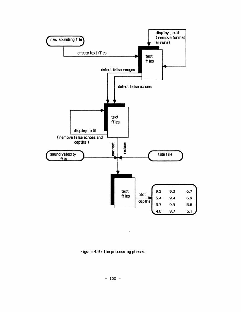
( raw sounding fil~
l create text files .. -detect false ranges
display , edit ( remove for mat
~r errors)
text files
detect false echoes
.. ..
display, edit (remove false echoes and
depths)
,, ,, text files
~ § t "i
( sound velocity ) 8 ....... '- ( tfde ffle ) filR ~f---------~~~------~ .. ..... , _____ _,
, text 9.2 9.3 files plot •
5.4 9.4 .. depths
5.7 9.9
'\.. 4.8 9.7
Figure 4. 9: The processing phases.
- 100 -
"""""' 6.7
6.9
5.8
6.1

5. TESTS and RESUlTS
.5. 1 Tests description and objectives
Jhe purpose behind these tests was to determine the feasibility of using personal
computers to perform marine survey and piloting functions. Each module of SEAHATS was
separately tested and the final test was devoted to the behaviour of the complete system. The tests
conducted were :
1. fredericton. Januarv 1984. Land trials were done to check the communication between
subsystems, the abi11ty to track rapidly changing Mini Ranger ranges and to give an estimate of
~namlc and static accuracy of the system. Peters ( 1984) describes this test.
2. Back Bav. March 1984. The stStem was tested aboard the vessel Mary 0 (a 13 metres
general purpose hydrographic launch owned by the University of New Brunswick) in rough see
conditions to evaluate its reliability and to check the effectiveness of the acquisition software and
the man/machine interaction.
- 101 -

3. Yarmouth I Mav 1984. An attempt was made to use the system for charting the
Yarmouth harbour waterway.
4. Fredericton I July 1984. The purpose of this test was to test the depth digitizing unit
and check if, under actual conditions, the digitized depths were in fact the true depths. Harris
( 1984) describes this test.
5. CamDQbello Island, June 1985. A sea trial was conducted during an actual survey by
the canadian Hydrographic Service (Atlantic Region) In the Lubec Channel between the state of
Maine and campobello Island (sea attached Figure 5.1 ). A network of six control points was
established and systems of survey lines were run as 111ustrated on the chart. Shoal ex81Tlinations
were performed using fictlclous shoal points using the "circles" and "star" maoos. The sea was
calm ( 0-1 Beaufort, Sea State 0), but there were strong tidal currents that Introduced strong
biases on the off-track errors. In ac:tJ1tlon, the ranges from West Quroty Head station were
heavily contaminated with spikes, probably caused by reflections from adjacent rocks. The
vessel's speed was 8-10 knots, while the maximum speed for the range filter was set at 20 knots
for reasons that will be explained later. The resolution of the echosounder was set to -22 em
(minimum pulse duration 0.3 milliseconds) and the receiver gain was adjusted to suppress heavy
shallow water background noise. When travelling at over 1 0 knots the echosounder lost the
bottom tracking, and the receiver gain needed readjustments. To monitor the tide, a tide station
was established at West Quroty Head and readings were taken e-~ery 5 minutes. The objectives of
the tests were to compare different navigation all}lrlthms for shoal examinations, to test the on
lfne modification module and to acquire data for testing the post-processing package.
SEAHATS was also tested using an ED:Iitional Apple lie computer that simulated the
position and depth data supplied to the vessel at sea. The simulation package was designed to
simulate shoal examination using the "circles" mode and the primary survey lines using parallel
straight lines.
- 102 -
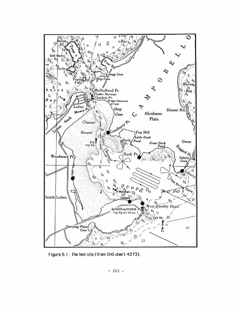
~ C., Abrahams
Plain
47
F1oure 5. 1 : The test site (from CHS chart 4373).
- 103 -
5.2 Accuracy
The 8::Cllrf:LY of the system was tasted for 8::Cllrf:LY of X ,Y and Depth measurements and for
its ability to l<eep constant time and distance intervals while Joooing soundings.
Test No. I (Peters, 1984) showed that the system can trocl< effecttvely Mini Ranger
ranges at the speed of 50 l<m/h, much more than the speed of a survey vessel (- 15 km /h ). The
uncertainty in the results is almost fully due to the Mini Ranger observation errors. The
uncertainty in position, for 1JXX1 geometry ( 90° intersection of LOPs), is !4.5m which can be up
to ±15m for bad geometry ( 1500) ( semi-d18(Jmal axis of error diamond). As expected the
observations were contaminated with spi!(es as shown In figure 5.2. The position fnter !(ept troc!(
of these range spi!(es but It lost trocking when It was not Initialized with ai}XX1 set of ranges. for
example, if the navigation function stopped and the b08t drifted, the filter had to be reset.
The depth digitizing unit was tested in test No. 4. Harris ( 1984) concluded that
depths derived from this digitizer agree with the internal echosounder digitizer within .:!:50 em.
The depth readings were stable.
figures 5.3 and 5.4 show two echograms and their digital representation. The sea
conditions of test No. 5 allowed safe interpretation of the echograms, since the foctors (such as
roll, pitch and heave) that affect depth 8::Cllracy and not considered In the system design , were not
present. The analog profile was constructed with a sampling rate of 600 soundings/minute and
the digital profile with 20 soundings/minute. We notice the following:
I. The direct effect of reduced sampling rate is that the system cannot tr~l< saa bottom
undulations of the order of 3 seconds (see echo return 2 on Figure 5.3). Here lies e disadvantage of
the on-line range rejection technique. If the position filter rejects range observations (e.g. for 6
- 104 -

2400 I l I I I I I I TT-T TT II I I I I J J J J J I I I I ; I I I I ; I I J I I I ; I I I l I j J I i I i I I I I I I I
r
Cl
n 2300 9 e
i
n 22CO t-' 0 V1
m
e +- I \ range spike c..
r 2100
e
G
:~ooo
1 1. 7 1 1. 8 11. g 12 J. 2. 1
time in hours
Figure 5.2 : Tt me aeries of ranoe from channel B of Mt n1 Ranoer.
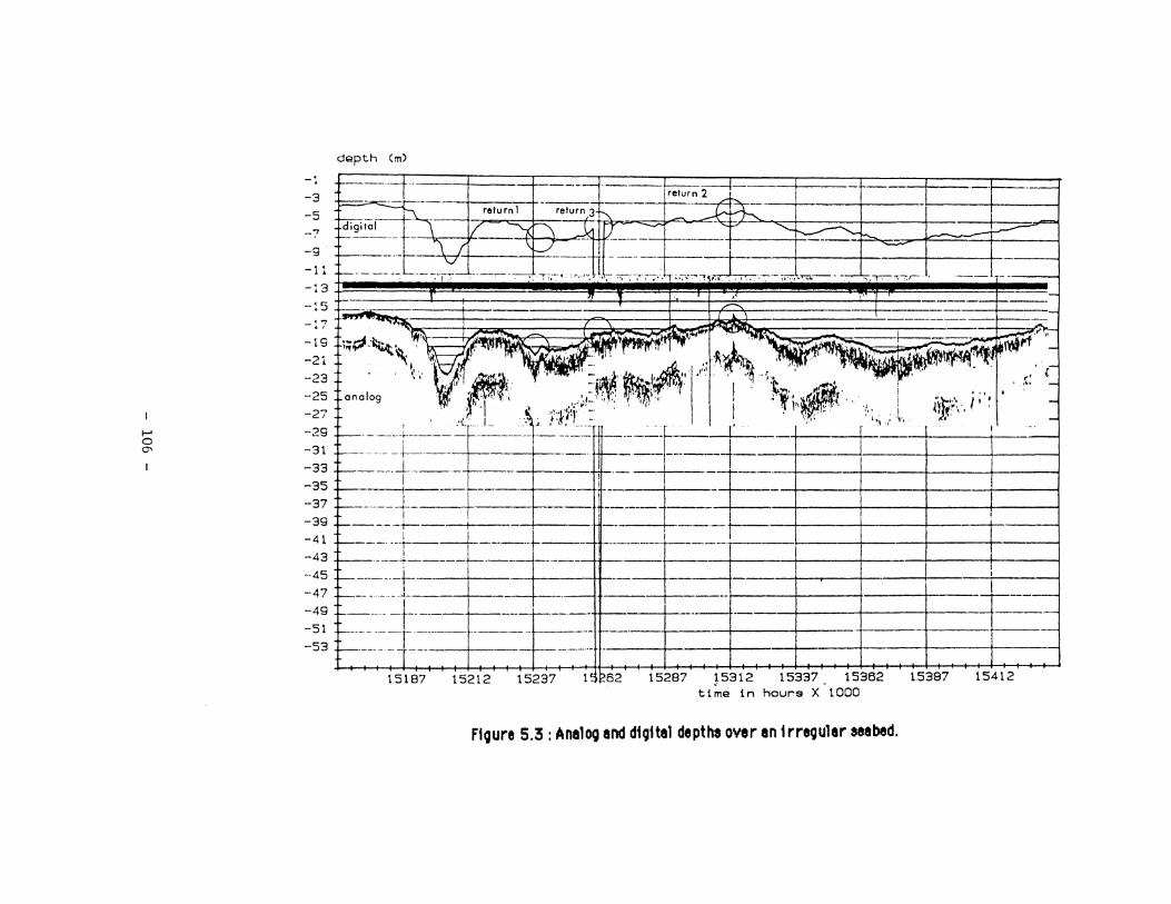
depth (m)
-3 -5 -7 -9
-11
~-- ·i·· --1--- ·- -- return 2 ··j· ~=-=-::::·-- ----- ---r--- ....... ~---. . -!----+----~- , _ returnl return 3 "'\ ~~ !
~g-to-!:1 >( ~~. ~ ~~:~~---.,..-..,-,;~ -~.~::c~ . -~ -13 -!5 ~- " , •" --1-.___ --:7 -19
-21 -23 -25 -27
I-' -29 0 0\ -31
-33 -35 -37 -39 -41 -43 -45 -47 -49 -51 -53
,...,..,. ,.,~ !... - '----·..;..
i;~--~~--r~\;~~·-~~r~~~r"· . -~-1 ~~~~~~~ll~l''~"~ ., , -~ ''¥. __,~ - ~ . . ~'ij;~ :l~Wi 'f . ')IJ.~..,q••r"•'11_ . _ ~ ' f
1'· l., ff1l4_''· • 'I'J.I~' ·-.~···~ _.,. •'''I • ~~ .f
1 ,., I' I t
I • .. • u · .. r :L ·,, . '"-~ · \' I .. ·-~,. ~t· j • •• • • .t. -one og · 1 _ 11 ·._
1 ..... i ,.•,, __ ·. :, ·.' · · ., ·1• -,. ' ~ •1 • , ·, · i i~'t··' /' • -
. I . ~-, ••. ,_.~·:,,·. ··-· . • • I ·. 'I . r ... .,_. i ,~,.·~·.·. . . I t ... ~------~- -~·~ ·__;_ /-:~.'-·----~-:- ···-- .. I . .. . .. __ ,:; _···~:\,.~-h •.. 1 -
~-- -----t------ -1--------- -- ---- 1---------~- _l ~-± :==----~+~----=-:=--~-I~---- ~:==---,-------=F=i - ---+-----l---~~~-:=== 1---------j----~------ ---- -- J -~--==~~---- '---- ~-= ------4----r-- - I
~~~~r---±~------~~------= :_ __ - 1 E--f---------+- ·- -- - I I I
1----- -··t---t-------1----·- -- ----- - ----~----·-· _, __ ---- f-------1------- t----1-------- .
1----- ---r ------ ------ ·-+------- t------ r------+-----+----+---- I ~------ -- -r--- --~----------
15187 15212 15237 1' 262 1528 time in hours X 1000
Ftoure 5.3 :Analog and digital depths over ant rreoular seabed.
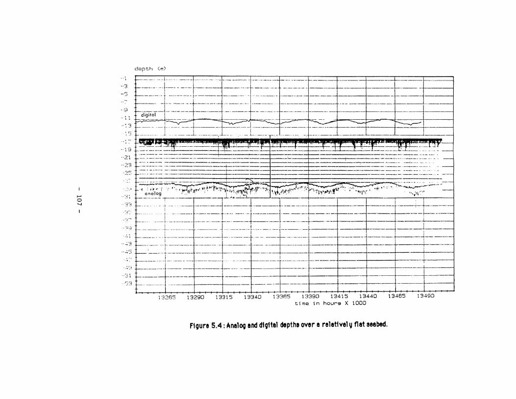
t--' 0 ..__.
depth (m)
....
E==~ ~-~1~=~-~-=~~1=~--~~~~t===~t===--~-~t:_~~-===·:r--=-~--t~=-T-=---t==-~+-------1 ------ j· ----------~----1--------l-- ------l------·---J------=-r-=---l- -
--3
-5
~---- -1--------·- --+--------------+----· --------------·---------+-------+------+--------f---+------·S.4
- i 1
-:3 --:5 .. ~ :~
--i9 ----21 --------· -- ___ .;_ ___ ---·- ....... - .. .
--+--· ----+-.....,..----------·- ----------~---- ······-. ----23
·25 ---· ···-- --- ------- ---·-----~---·-·---·--··- --~~~~---. . I -----~-~-------
.:·,4 ·( .i ,·~··1 ··: •·,.,.,_.1/r';t~t•'··~·~"'tl•:.\f•)l,),.,4.,~f;11'"':~: ,;.. ••,'rl····• ---
·;~ :._,~~~ 't: ~- ~ __ E--l~~· -~"+==---=lt.- --_----=t----~---~=----f---- -~- ~-b_ .. -_.... ----- --i·-----r~==:--r·------1-----~----------~------- --f-- ___ _J ____ _ .. -_ .. "] -----+--------- --- I--------~-----·.=r---·--- -- ---- ~
~; --==~-t-~=~ --=· -~f~·-:=+-~=t~-~~~~-=~~~- -==~=t==~ · r=~r-;:=--=------l~-~--:_-_-- :~±J --_-____._± __ _
. -~ ~~ -·:J 1
. ·':i:-3 I
13265 13290 13315 13340 13365 13390 13415 13440 time in hours X 1000
Ftoure 5.4: Analoo and dtottel depths over a relettvel"' flat seabed.
13465 13490
seconds), no depths are recorded during this perloo, although depths are g:m (see echo return I
on Ftgure 5.3). Thts ts why It is preferred to set wide range rejection tolerances and use an off
line fflter to further smooth r~.
2. The percentage offalse echoes is extremely small. In echogram of 4 hours length, only
once did the digitizer pick up an echo other than the sea bottom. On the other hand, echoes such as
shown in Figure 5.3 (echo return 3), are common. These, as mentioned earlier, are caused by the
echosounder tranceiver not receiving any return from the sea bottom.
3. The rest of the digital output agrees very well with the analog treK:e. The mean
agreement is in the order of 30 em.
4. It is difficult to attribute the sawtooth effect appearing on the echogram of Figure 5.4
to the effect of ship motion ( roll,pitch and heave), even when the seabed is relatively flat. The
reason is that the magnitude of this effect is in the orrer of vertical resolution of the echosounrer
(22 em).
It must be emphasized that the above echograms are easily interpreted. The echo returns
from the first bottom are strong enough to stop the digitizer cloc~. However, the behaviour of the
digitizing unit in deeper waters, or in muctty seabeds, or in a seabed covered by weed is not
guaranteed. More tests unrer these conditions are required.
Selection error. Hydrographic survey operations require precise and consistent data
logging of navigational and bathymetric parameters at specific distance or time intervals. The
desired accuracy in time and distance intervals is an unbiased mean error of nearly zero and a
sample standard deviation of one second or less. Two ffl:tors IJ)Vern this precision : the
computational speed (cycling time) and the observation sampling interval.
For SEAHATS, cycling time increases proportionally with the number of data points that
remain In the PSO 1 Interface buffer (see also Figure 3.5 ). This Is done as the Interface software
- 108 -
continuously transfers data points until it receives a recent one. This amount is n X dt, where n
represents the number of remaining data points In the buffer and dt the time required to transfer
a point c-o.70secat 1200 baud rate). For example, if the sampling Interval ts 1 second, after
six cycles 6 points remain in the buffer, and the total computation time is 2.3 + 6 XO. 70 = 6.5
seconds. But during thts time, more points enter the buffer. Figure 5.5 gives a comparison of the
computation times for samp11ng Intervals 1=1,2,3,4, .... The minimum computation ttme exists
for a samp11ng Interval of 3 seconds (approximately equal to data manfpulatton time). This
ensures that the rate of incoming data in the buffer, equals to the rate of exiting data.
Another alternative for requesting data from the buffer would be to erase all the data
points and then request. But if the request is done at the beginning of the sampling interval, the
computation time is increased by the sampling interval. In this case, the cycling time is 4
seconds (assuming minimum sampling interval 1 second).
The cyclfng ttme of 3 seconds therefore restricts the minimum ttme selection Interval to
3 seconds or distance interval of 12 metres at 8 knots. It ts also expected that the error in time
intervals will be in the order of 3 seconds. Attemps to reduce execution ttme Include :
(a) reduce the time required to write on the screen,
(b) produce more efficient code,
(c) switch to a different faster operationg sytem, and
(e) use an additional processor to partially off-load the 6502 microprocessor.
The Apple lie has a memory mapped screen. Writing directly on the screen is faster.
Benchmark tests showed a reduction factor of 3. However, this approach destro,ts the flexibility
and machine independence of the system and therefore it was not adopted. For the same reason,
coding of Least Squares adjustment ( the most time consuming routine) in assembly langu• was
not ad:lpted.
- 109 -
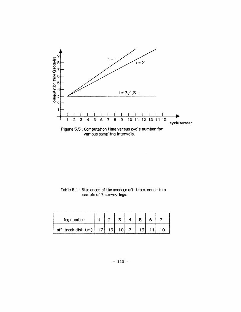
i = 3,4,5 ...
2 3 4 5 6 7 8 g 10 11 12 13 14 15
Figure 5.5 : Computation time versus cycle number for various sampling intervals.
Table 5.1 : Size order of the average off-track. error in a sample of 7 survey legs.
leg number 1 2 3 4 5 6 7
off-track dist. ( m) 17 19 10 7 13 1 1 10
- 110 -
cycle number

To each successful range measurement the closest In time depth measurement Is attached.
The depth digitizer Interrupts the Interface central processor and provides depth Information
approximately rNery 100 milliseconds, leMing to a position and depth correlation in the order of
I 00 milliseconds (or 50 em at I 0 knots).
5.3 Man/machine interaction
A second monitor was required to display information to the helmsman. Unfortunately the
command and situation displays could not be separated and the screen contained too much
information. This caused some problems to the hell'nsman. These were overcome following some
familiarization with the display.
The track keeping ability of the system lies in its ability to keep small offsets from the
survey leg. As mentioned before, the cycling rate of the l/R indicator, its resolution, the vessel's
speed and turning characteristics, and the helmsman's experience in conning survey vessels affect
this ability. The L/R indicator has a resolution of Sm. There is no need to keep finer resolution
when the position accuracy is in the order of 5 metres. Figure 5.6 shows ship's tracks steaming at
8 knots and with line spacing S=SO metres. The survey boat was navigated by an experienced
operator.
In order to measure this abtlity, the area E bounded by the ship's track and the desired
track Is calculated (see also figure 5.6). The segment of survey leg, which is used for ship's
turns, must not be included in the calculations. If the length of the survey leg is D, an average
deviation from the desired track can be computed by:
m = E /0 (5.1)
- 111 -
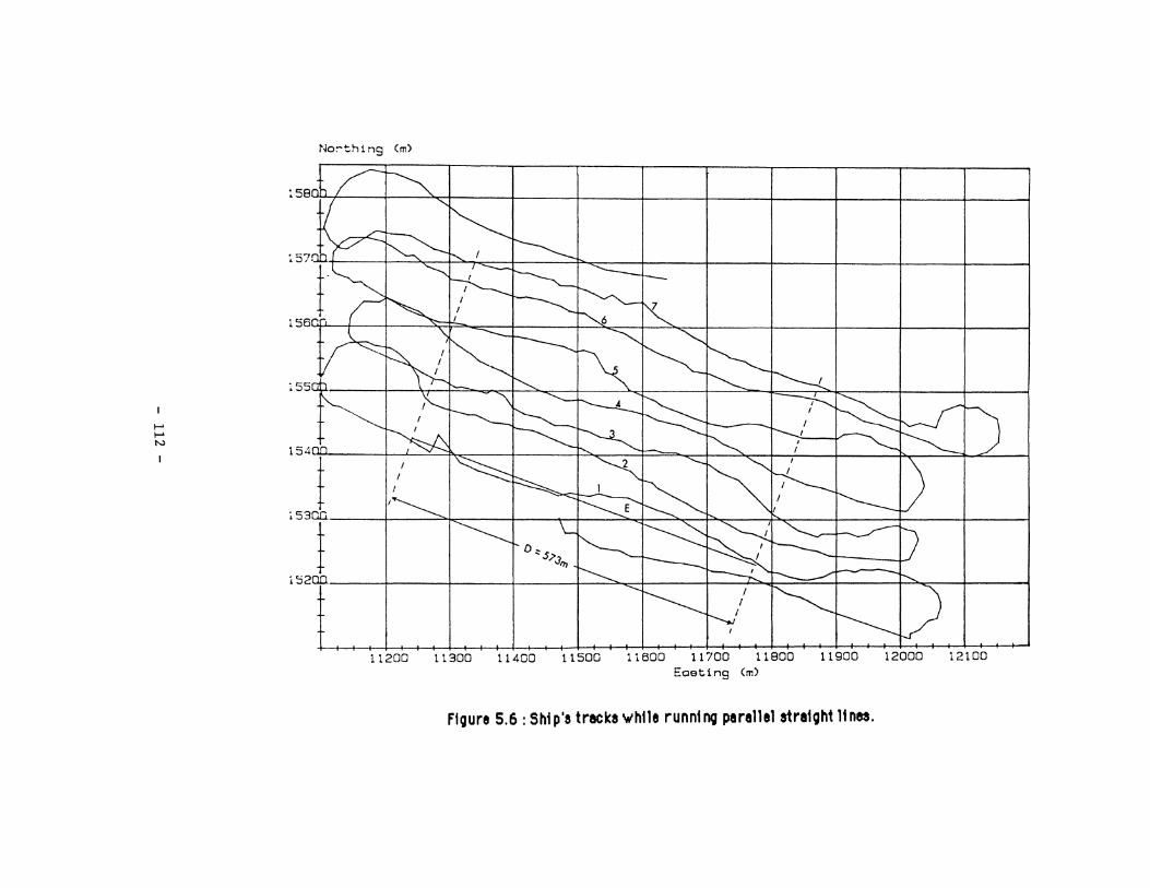
t-' t-' N
No~th i ng (m)
11200 11300 11400 11500 11600 11700 11800 11900 12000 12100 Eaeting (m)
Figure 5.6 : Shi p'a traclca 'w'h11e runnt ng parallel straight 1t nea.
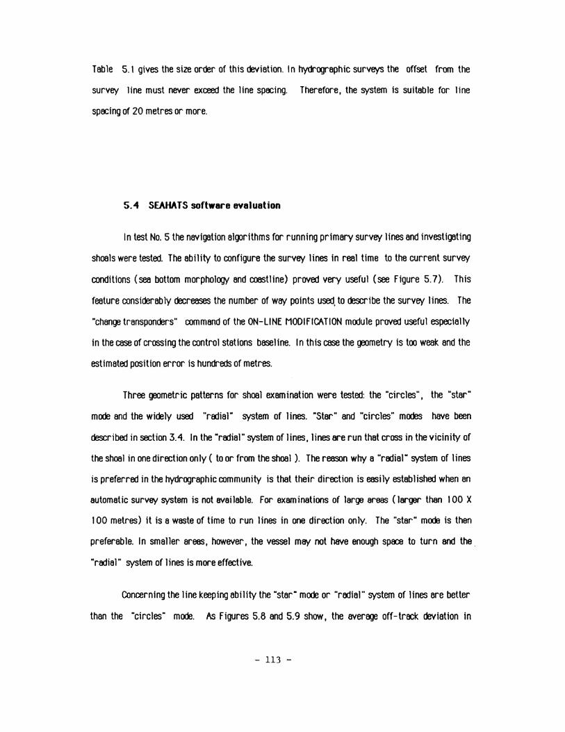
Table 5.1 gives the size order of this deviation. In hydrOJraphic surveys the offset from the
survey line must never exceed the line spacing. Therefore, the system is suitable for line
spacing of 20 metres or more.
5.4 SEAHATS software evaluation
In test No. 5 the navigation al~rithms for running primary survey lines and investigating
shoals were tested. The ability to configure the survey lines in real time to the current survey
conditions (sea bottom morpholCXJY and coastline) proved very useful (see Figure 5. 7). This
feature considerably decreases the number of way points Used, to describe the survey lines. The
"change transponders" command of the ON-LINE MODIFICATION module proved useful especially
in the case of crossing the control stations baseline. In this case the geometry Is too weak and the
estimated position error Is hundreds of metres.
Three geometric patterns for shoal examination were tested: the "circles", the "star"
mode and the widely used "radial" system of lines. "Star" and ·circles" modes have been
described in section 3.4. In the "radial" system of lines, lines are run that cross in the vicinity of
the shoal in one direction only ( to or from the shoal ). The reason why a ·radial" system of lines
is preferred in the hydrOJraphic community is that their direction is easily established when an
automatic survey system is not available. For examinations of large areas (larger than I 00 X
100 metres) it is a waste of time to run lines in one direction only. The "star" mode is then
preferable. In smaller areas, however, the vessel may not have enough space to turn and the.
"radial" system of lines is more effective.
Concerning the line keeping ability the ·star· mode or "radial" system of lines are better
than the "circles" mode. As Figures 5.8 and 5. 9 show, the average off-track deviation in
- 113 -
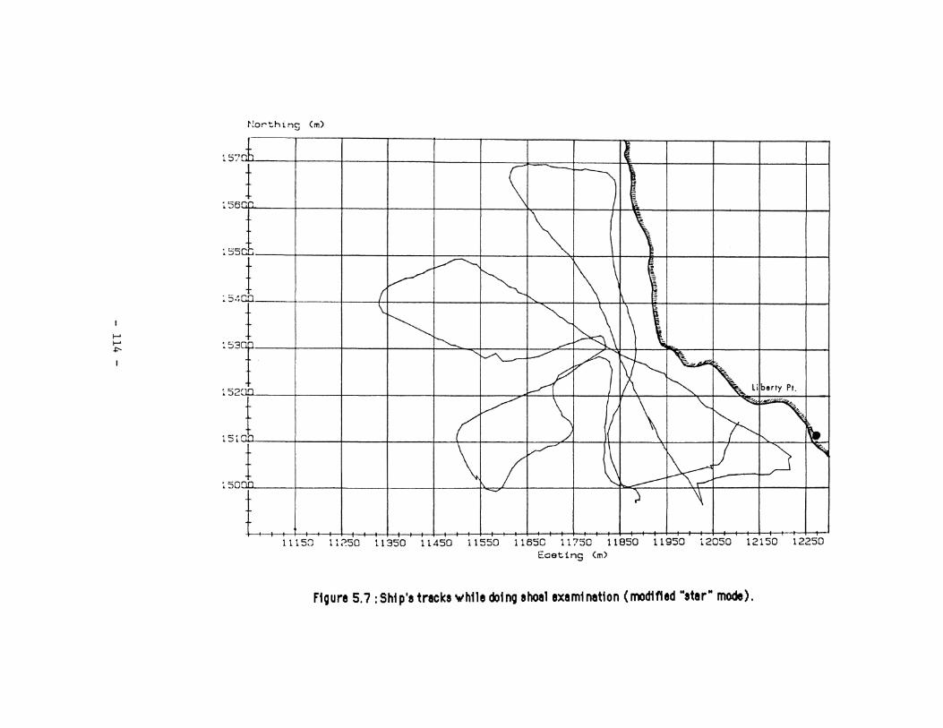
......
...... ~
~-1ort.hins <m)
157 l I~
156 t \ I •
"' ~ \ ;cf _,..-.---J---" --., [\ \ \
+ I ~~ I\ I
155
on \ ~ \\ i ~~ ---~ -T ~~[::? r f\0- '-~ -
/ 1/\ ~ ~ liberty Pt.
:54
153
152
t /v \ II \ "'~" '~ ;nt f / II .....
± \ /~ ~ --k~-----+--" 151
1nh ~ ) ~
L ......... -~-~~~~ 150
11150 11250 11350 11450 11550 11650 11750 11850 11950 12050 12150 12250 Eaet.ing (m)
Ftgure 5. 7 : Sh1 p'a trecka 'w'htle dot no shoal examt nation (modified "star" mode).

t-' t-' V1
~-iort.h i ~19 (m)
:6~GC; __________________ ~-----7L_---,L---~------------~--~------------------i--------l
, oc.~ . ~~~~-------------------------~----------------------------t---------------------------t---------------------------~------------1
10000 1Sl00 10200 10300 Eostt ng (m)
F1Qure 5.8: Ship's trecks 'w'h11e do11'19 shoal examination ("circles" mode).
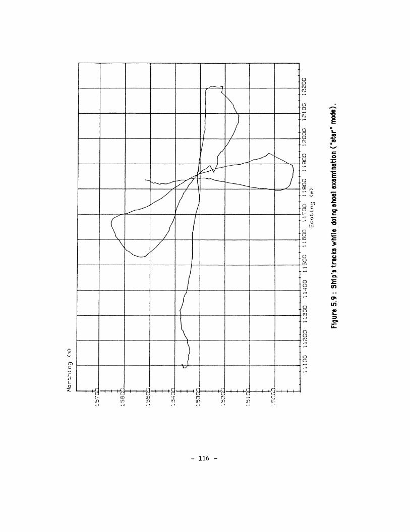
m c ·~
.r: ., (_
0 ":<:. r
( {•.
;n
\
I I
\
l I<. (() !n
-1-----
~ v I
~ /
t~-~--+-+? ill tn ·~ 1n
-- _, (
I
I (
c:::v-A vi --
1/ L I
I I \
I >.J
--+--+-i t~ I I ,c. c
(T) lfl
- 116 -
\ )
v
f-
r------
-+-+-+c (
__./"
""
'8 c lf,
)
0 0 (\J ('.j
0 0 0 (\J
0 0 Ol ....
0 0 w.,.. -~ E -· V'
m g c (··. :; .... (,') .~ u
0 0 (()
0 D IJ1
l:l
-I • L
B ., • -c 0
~ c
e .., ~
i ., ~ i 41) -:E ):
~
f -_., a.
0 :E l1 (I) -. -0 0 (T)
0 (.) (\! ....
0 0
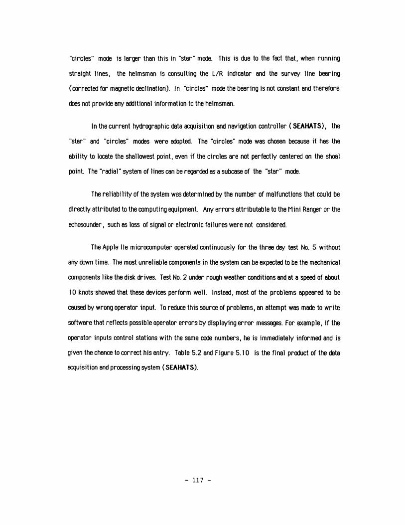
"circles" mode Is larger than this In "star" mode. This Is due to the fact that, when running
straight lines, the helmsman Is consulting the LIR Indicator and the survey Hne bearing
(corrected for magnetic declination). In "circles" mode the bearing Is not constant and therefore
does not provide any oo:Jitional information to the helmsman.
In the current hydrographic data acquisition and navigation controller ( SEAHATS), the
"star" and "circles" modes were 800pted. The "circles" mode was chosen because if has the
ability to locate the shallowest point, even if the circles are not perfectly centered on the shoal
point. The "radial" system of lines can be regarded as a subcase of the "star" mode.
The reliability of the system was determined by the number of malfunctions that could be
directly attributed to the computing equipment. Any errors attributable to the Mini Ranger or the
echosounder, such as loss of signal or electronic failures were not considered.
The Apple lie microcomputer operated continuously for the three day test No. 5 without
any cklwn time. The most unreliable components in the system can be expected to be the mechanical
components lllce the dislc drives. Test No. 2 under rough weather conditions and_ at a speed of about
I 0 knots showed that these devices perform well. Instead, most of the problems appeared to be
caused by wrong operator input. To reduce this source of problems, an attempt was mroe to write
software that reflects possible operator errors by displaying error messages. For example, if the
operator inputs control stations with the same code numbers, he is immediately informed and is
given the chance to correct his entry. Table 5.2 and Figure 5.10 is the final product of the data
acquisition and processing system ( SEAHA TS ).
- 117 -
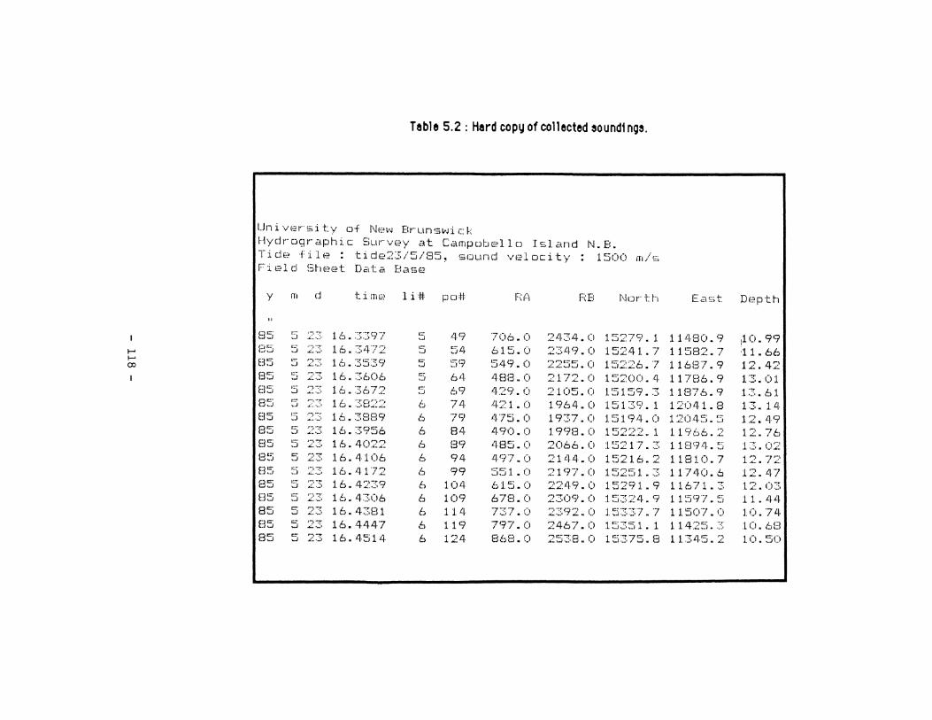
Table 5.2 : Herd copy of collected sound1 ngs.
University of New Brunswick Hydrographic Survey at Campobello Island N.B. T:ic.i&:! +ilc·? : tidf?2:J/5/85, scJLmd velocity : 1500 m/~:; Field Sheet Data Base
y m d t :i filE-) l i :It po# F((\ rm NDI'""t.h Ea~:;t. Depth
II
f.35 ~::; 2~:; 16. :::.:::.97 o:::- •l9 706.0 2434 • 0 1.5::~7CJ. j_ 11LI-80. 9 :10.99 ,..J
IB:3 ~5 z.:;; 16. ::H72 c::- 54 615.0 2349.0 15241..7 11582.7 ;11. 66 1-' ,..J 1-' B:S 5 2::: 16 .. 35:39 r.::" !=:"(;:) 549.0 2255.0 15226.7 11687.9 12. 4:~ 00 ,..J •. .1 1
85 ~..) ::3 16. :3606 1:~ 64 48!3. 0 2172.0 15200.4 11786.9 1.:::.. 01 I ,..J
E:l5 5 2~.) 1tS .. ::::.t.;7~2 ·:::· ,..J 69 429.0 2105.0 15159.3 11876.9 1:3. 6l 8:'5 ~5 =~~:. 16. ::::s::2 6 74 421.0 1964-.0 151::::9.1 1204-1.8 1:::.. 14-E:l5 !:5 23 16. 38!39 6 -](:)
' 1 lJ.?~i. 0 1937.0 1.5194.0 12045.5 12. 4-9 85 ~:.; 2:3 16.::::956 6 84 490.0 1998. 0 1 ~322:2. 1 1.1966.2 l.2.7b B5 ~.:i 23 16. •l022 6 B9 •lB!:i. 0 2066.0 15217.3 11894.5 1:::.02 85 5 ::3 16.4106 6 94 4-97.0 2144.0 15216.2 11810.7 1,.., --,~.\
,.;.. • I .:...
E35 ::::; ~.:::3 16.4172 6 99 ::i51. 0 2197.0 15251..3 11740.6 1~?.4-7 85 ~3 :::5 l. 6. 4239 6 104- 61.:"..). 0 2249.0 15291..9 11671.3 12.03 fl5 ~3 ::~::: 16. 4:306 6 10<1 67B.O 2309.0 15324.9 11597.5 11.44 85 5 2::. 16. 4::.81 6 1l.ll 7::.7. 0 2:::.92. (l l. ~5::.:::.:::7. 7 11.507.0 10. 7lJ. B5 5 23 16.-444-7 6 119 797.0 2467. 0 1:':i351. 1 1142:3. ~:. 10.68 85 5 :::;~ 16.4-514 6 124- 868.0 2538.0 15375.8 11345.2 10.50
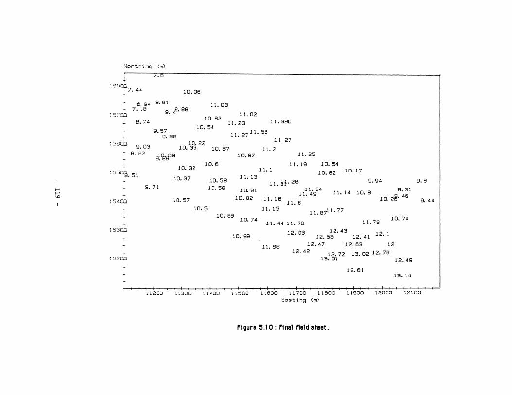
t-' t-' \0
Nort.ht ng (m)
• '<8"r. -~-~7.44
t 6. 94 B. 61
t '7.1 8 9.P· 88 11.62 1 '37GO .10. 82
10.06
11. 03
11. 880 t 6 74 .11. 23 • 10.54
9. 57 11. 27 11. 56 9. 88 .11. 27
. "'"00 10.22 ·-~ 0 9.03 10."35 .10.67 11.2
t 8. e2 dW9 10.97
:'55~. 51 i 9.71
154! 153GO
t 15200
10.32 10.6
.10. 37
.10. 57
10.5
10.58
10.58
11. 13
10. 81
10.82
.10. 68 10. 74
10.99
11.25
.11. 19 .11.1
11. !t· 26
10.54
10.82 10. 17
9.94
11.34 11. 1 B 11. 49
.11. 6
11. 14 10. 8 9. 31
.10.2~.46
11. 15
11.4411.76
12.03
11. 8r 1. 77
11. 73 10.74
.12. 43 12. 58 12. 41 1 2· 1
11. 66 12.47 12.42
12. 63 12
12.72 13. 02 12. 76 13. 01
13. 61
12.49
13. 14
9. 8
9.44
11200 11300 11400 11500 11600 11700 11800 11900 12000 12100 Eaettng (m)
Figure 5.10: Ftnal fleld sheet.

6. CONClUSIONS and RECOMMENDATIONS
The results of the tests indicate that a microcomputer with commercially available
peripherals and standard software, such as the Apple lie, offers great promise of replacing
larger and more expensive hydrographic data acquisition and navigation controllers. Personal
computers are alreOO'y' used in marine applications. Stoltz et a/. ( 1985) use the IBM PC
personal computer integrated with Loran C and Del Norte Trisponder for geophysical surveys. The
computational all}lrithms exist and need only to be modified or simplified to fit the memory
capacity and computational speed of microcomputers. The memory requirements (RAM) for
SEAHATS acquisition software is of the order of 60 !<bytes which is not readily available on 8 bit
microcomputers. Memory overlapping techniques must be used to fit the code into the memory
capacity of an 8 bit computer. Alternatively, use of a 16-bit or 32-bit computer would overcome
this (and several others) SEAHATS limitations- but at increased cost.
The factors which created the greatest difficulty in reveloping an automated system were
the development of specifications, the computer memory and computational speed constraints,
and compliance with man/machine Interaction specifications. Considerable programming effort
was required in the man/machine interface routines.
- 120 -
Throughout the developing phases the following conclusions were reached :
1. If we want to rani< the criteria for choosing a position or range filter for use in the
hydrographic surveys that use low cost microcomputers and pulse matching microwave
positioning systems, the following list (from higher to lower priority) must be atbpted (slight
rearrangements are allowed):
(a) computational burden (e.g. Kalman fi Iter requires heavy computational burden),
(b) implementation cost (e.g. mu It iranging requires the operation of Bliiitional control
stations),
(c) gross-error detection,
(d) smoothing ability and
(e) dynamic response.
According to the above list, simple gating techniques or linear filters seem to be preferred.
2. The need for a depth filter and its degree of complexity depend on the specific digitizer
echosounder system and the area of application (water depth, sea bottom morphology). Simple
comparisons of digital and analog depths are effective methods to detect false echoes.
3. The system of survey lines must be able to be altered on-line to suit the current
configuration of the shoreline and sea bottom slope. Frequent OOjustments, however, must be
avoided because they tend to confuse the launch hydrographer and coxswain, since they oo not have
a clear picture of the survey lines run. In ack11tion, If the changes are not well lilcumented,
problems can arise in the interpretation of results while post-processing the data.
4. The "star" mode is the best shoal examination pattern with respect to track keeping
ability if the location of the shoal point is accurately known.
5. Applications that require very closely spoced sounding lines ( 10 to 20 metres) cannot
be satisfied by the present configuration of the system. The limiting factor is the accuracy of
- 121 -

positioning system and the 3 second update interval of the command display. However, the
navigation and processing algorithms are suitable for these applications.
Recommendations for further development of SEAHATS, as a specific hydrographic data
acquisition and processing system are:
1. Since the computational burden Is of vital lmoortance, the depth f11terlng technique
discussed in section 3.3.4 can be implemented In hardware inside the digitizing unit.
2. The Kalman filter developed in section 4.3.1 can be implemented on-line and the
increased computational burden measured. The filter will provide real time stabilized estimates
of the velocity over the bottom ready for use in the range rejection techniques.
3. Ways of uninterrupted data loootng when the storage device becomes full must be
investigated.
4. A trock. plotter used as l/R indicator can result in better trock. k.eeping ability.
5. Investigate different ways to specify the area to be surveyed. Boudreau (I 985)
suggests that the chart limits (that include the area to be surveyed) be stored In the computer.
Then the chart is subdivided into a set of polygons, which also are stored in the computer.
finally, in eoch polygon the lines to be surveyed and the shoals to be examined are specified. Eoch
sounding is occompanied by the chart, polygon and line numbers and therefore its position in the
Hydrographic Data Base is easily specified.
6. The following utilities will further simplify the job of launch hydrographer :
-an interoctive network. design pack.age for optimizing horizontal network.s in order to
choose the best sites for the Mini Ranger transponders,
- a coordinate transformation pock.age between map projections,
-a calibration poclcage using baseline crossing, and
-a pack.age for pre-plotting of Mini Ranger lattices.
- 122 -

7. The current ocquisition software can be interf~ to a high ~J:CUracy range/bearing
system for use in marine construction surveys.
The foJJowing recommendations (not specificaJJy to SEAHATS) are also m~:
I. Techniques to 1oont1fy liKely shoal areas between sounding lines, and methoos to
ootermlne optimum line spacing and sounding Intervals In the primary survey lines and while
Investigating seabed features must be developed.
2. The existing depth filtering techniques require testing. New techniques must also be
devised. For example, one technique would be to fit a high order polynomial to the sea bottom, or
to correlate the I st and 2nd echo returns from seabed and occept the echo returns with high
degree of correlation.
The features of the developed hydrographic data acquisition and processing system
(SEAHATS), can be fully explored if we are aware of its Jimltatfons. These limitations mainly
are: (a) the stage of complete automation In oopth acqulsltfon has not been ldlieved. The echogram
conveys much more Information than the digital oopths and It is always necessary to compare
digital and analog depths, (b) the system is unable to run closely sp~ survey Jines and (c) in
the case of computer malfunction or power failure the data files are lost. The software (or
hardware) 00es not make any provision to save them.
- 123 -
LIST OF REFERENCES
Aboh, C. E. ( 1983). Evaluation of Tidal Water Level Transfer Techniques for Land Surveving. M.Sc. Thesis, Department of Surveying Engineering, Unfvers1ty of New Brunswick, Fredericton, N.B., CanEKia, 91 pages.
Attwood, E.L. end H.S. Pengelly ( /967). Theoritical Naval Architecture. LongMans bublfcatfon, Lonoon, pp. 283-288.
Bergen, A. W. ( 19 79). Increased Accur~ and Relfabllfty fn Offshore Posftfoning. Proceedings of the 6th ttvdrooraohic Survey Conference, Vicksburg, Miss., December, pp. 175-199.
Bertsche W.R., Cooper R.B., Feldman O.A. end Schroeder K.R. ( 1981). An Evaluation of Display Formats for Use with Marine Radio Navigation Piloting Systems. Navigation: Journal of the lnstitude of Navigation. Vol. 27, No. 2, Summer, pp. 116-123.
Bomford, A. 8. ( 1962). Transverse Mercator.Arc-to-chord and Finite Distance Scale Factor Formulae. EmoireSurvevReview. No. 125, Vol. XVI,July, pp. 318-327.
Boudretlu, H.A. ( /98"1). Specifications for a HydroorBohic Aguisition and Navigation Controller. Undergraduate thesis, Department of Computer Science, Acadia University, April, 92 pages.
Bowditch, N. ( 19 7 7 ed.). American Practical Navigator. Volume 1, Defence Mapping Agency HydreJJraph ic Center , Publication No. 9, p. 721.
Bryant R.S., Ooekes C. end Tripe R.L.K. ( 1976). INDAPS, Integrated Navigation, Data Acquisition and Processing System. International ttvdrooraohic Review, Monaco,llll(2), July, pp. 65-85.
Casey, 11. J. ( 1981). Range Aa:.urtry and Signal Strength in Motorola Mini-Ranger System. Proceedings of the 20th Annual Canadian Hydrographic Conference, Ontario, pp. 37-49.
Casey, 11.J. ( 1982 e). Multiranging - An Expensive Solution to a Simple Problem. Lighthouse: Journal of the Canadian Hydrogroohic Association, Edition No. 25, April, p. 41.
Ct1sey, 11. J. ( 1982 b). Improving Quality Control Trhough Real Time Statistical Filtering. Proceedings of 41b. International Sumoosium HYDRO '82, Volume 3: Data Acquisition and Processing, Unfversfty of Southampton, England, 23 pages.
C/oet, R.L. ( 1984). Where have all the data (Jme. MethOOs of Dfsplav of Ck:eao Suryev Data, edited by Ron Linton, NERC Thematic Information Setvice, England, pp. 14-37.
Cross, P.A. ( 1981). The Computation of Position at Sea. The Hvdrooraohic Journal, No. 20, April, pp. 7-16.
- 124 -

Oel Orosso, Y.A. end C. W. /'Ieder ( 1912). Speed of SOund in Sea-Water samples. Journal of the Acoustical Societv of America, Volume 52, February, pp. 961-974.
Oronkers, J.J. ( 1964). Tidal Computations in Rivers and Coastal Waters. John Wiley and SOns Publication, New York, pp. 3-24.
Eestwood, A.R. ( 1984). Early Applications of Civil OPS. PLANS' 84: IEEE Symposium on Position and Naviaation, San Diec}l, California, November, 12 pages.
Eeton, R./1. ( 1984). Sounding Nxurooy. Atlantic Oceanooraohic Laboratorv, Bedford Institute, Internal note 1968-18-1.
Eeton, R./1. ( 1968). Smoothing and Mult-Ranging. UQhthouse: Journal of the Canadian HydrooraphicAssociation, Edition No. 25,April, pp. 39-40.
Enebnit, 0. ( 1985). Shipboard Data Systems Ill. Proceedings: Hydrooraphy and Technology in the Mid-80s, Ha11fax. April, (in press).
Felkengberg, W. H. ( 1981). NAVPAK, an integrated system for navigation and positioning for offshore oil and gas exploration. Proceedings of Colloouim Ill on Petroleum Mappina and Survevs in the 80's. The Canadian Petroleum Association, Banff, October, pp. 175-194.
FlO lnternetlonel Federetion of Surveyors ( 1911). Working eroup 414a: Data Acauisition and Processing Svstems Prooress Reoort June 1977. Surveyors Publications, London, 95 pages.
FlO lnternetionel Federetion of Surveyors ( 1981). Work ina group 414a: Data AcQUisition and Processing Systems. Catalogue of Users and Vendors of Automated Hydrographic Survey Systems. FIG XYI Congress, Montreux, Switzerland, August, 287 pages.
FlO lnternetionel Federetion of Surveyors ( 1984). tfvdrooraphic Survey Equipment 1984 Catalooue. Surveyors Publications, LonOOrl, 349 pages.
Forrester, W.O. ( 1983). Canadian Tidal Manual. Department of Fisheries and Oceans, canadian Hydrographic Service, ottawa, pp. 55-64 and 101-111.
Oelb, A. ( 1914). Applied Ootlmal Estimation. The M.I.T. Press, Cembrili;Je, Mass., U.SA.
Oilb, T. P. end fJ. F. C. Weedon ( 1916). Range holes and what to do about them. Lighthouse: Journal of the Canadian HydrooraohicAssociation, Edition No. 13, pp. 2-5.
Oilg, J. (J. ( 1910). A Bathymetric Evaluation of Doubtful Hydrographic Data. International Hydrooraphic Review. Vol. XLVII, No. 1 • January. pp. I 13-121.
()rent, S. T. ( 1916). lntearatfon of Passive Ranofng Loran-e satell1te Navfaatfon. Ship's Loo and Ship's Qvrocompass. M.Sc. Thesis, Department of Surveying Engineering, University of New Brunswick, Fredericton, N.B., Canada, 106 pages.
()rent, S.T. end O.E. Wells (1983). lnter~~:tions among Integrated Navigation Systems. Marine Oeoc!!m'. Vol. 7, Number 1-4, pp. 153-170.
-•Hall, /'I.P./1. ( 1919). Effects of the troposphere on radio communication. The Institution of Electrical Engineers, London and New York. pp. 47-77.
- 125 -

Harris, J. ( /984). lnterfoce between the Slmrad Sklpoer 802 echosounder and SEAHATS. University of New Brunswick, Department of Surveying Engineering internal report, Fredericton, N.B., canada, 27 pages.
Hopkins, R.O. ( 1980). Heave-Roll-Pitch correction for Hydrographic and Multi-beam Survey Systems. Proceedings 19th Annual canadian Hvdrooraohic Conference. Halifax. March, pp. I 05- 116.
Hourdokis, P. ( 1985). OPerating Manual and Software listing for SEAHATS. University of New Brunswick, Department of Surveying Engineering, Technical Memorandum 8, fredericton, N.B., Can008, 178 p~.
1011 Services Ltd. ( 1982). Microprocessors based integrated navigation. reports : I, ( 21 pages + 8 appendices )
2, ( 20 pages + 4 appendices ) 3A, ( 9 pages + 2 appendices ) 4, ( 14 pages + 4 appendices ) 5, ( 8 pages + 16 appendices ) 6, ( 12 pages) 71 ( 19 pages) 8, ( 4p~)
fredericton, N.B. canada.
IHB International Hydrographic Bureau ( 1982). Standards for Hvdroocaphic Survevs and Classification Criteria for Deep Sea Soundings. Special Publication 44, Monaco, 1982.
Ingham, A. ( /974). Sea Surveying. McCraw Hill, New York, pp. 119-165.
Jones, H. W. ( 1983). The influence of mooaJJing errors on the oerfomance of the Kalman Filter. eradulrte Seminar I Department of Surveying Engineering, University of New Brunswick I
Fredericton, N.B., Canada, 15 p~.
Janes, H. W. ( 198 4 ). SEAHA TS li:!velooment considerations. University of New Brunswick, Department of Surveying Engineering internal report, Fredericton N.B. , Canada, 87 pages.
J/1R ( 1981). Introduction. System 21 products for lntergrated Marine Data Acquisition and Navigation Svstems. JMR Instruments Canada Ltd., Document No. 2100-00-0001, Rev. A, February, 14 pages.
Keyton, 11. and W.R. Fried ( 1969), editors. Avionics Navigation Systems. John Wiley and Sons Inc. New Yorlc., pp. 555-578.
L onghorne, 0. N. ( 1981). The Stability of the Top metre of the Seabed; Its importance to Engineering and Navigational Projects. Proceedings of the 20th Annual canadian Hvdrooraphjc Conference, Ontario, April, pp. 62-71.
Laurila, S.H. (1976). ElectronicSurvevingandNaviootion. JohnWileyandsons, pp. 130-134, 198-204and67.
Leenoorts, H. W. end R. C. Jellemo ( 1984). A software approach to reliability and resilience in hydrographic surveys. Proceedings HYDRO '84 National Ocean Service Hydrooraphic Conference, Rockville , April, pp. 156-159.
- 126 -
Lewis, N.C. ( 1980). The weed dilema. Proceedings of the 19th Annual Canadian tfvdrooraphic Conference, Ontario, March, pp. 94-104.
ttacdonald, 0.0. and tt.J. Casey ( 1915). Automation-the changing Roles in Hydr(XJ'aphy. Presented at the Canadian Institute of Surveying Annual Convention, Fredericton, N.B., Canada, April, 11 pages.
ttacdonald, 0. 0. ( 1981). The Use of Microprocessors for Tract. Control on Data verification on HydraJraphic Surveys in Canada. International Hydrooraphic Review. Vol. LVIII, No. 1, January, pp. 39-53.
ttacdonald, 0. 0. ( 1984). Computer- Assisted Sounding Selection Techniques. International Hydrooraohic Review. Monaco, LXI ( 1), January, pp. 93-109.
tfackay, J.tt. ( 1912). Automation of HydraJraphic Surveying. International Hydrographic Rev if'!', Vol. XLIX, No. 2, July, pp. 149- 166.
ttacPhee, S.D. ( 1919). Underwater Acoustics and Sonar and Echo Sounding Instrumentation. Canadian HydraJraphic Service, Technical Report No. 1, April, 94 pages.
ftalone, A. K. ( 1984). Digital Data Base Management for HydraJraphy. Proceedings HYDR0'84 National Ocean Service tfvdrooraphic Conference, Roct.ville, April, pp. 151-155.
ftarlln, J. (1913). Design of Man-Computer Dialooues. Prentice-Hall Publication, 559 pages.
ftatthews, 0. J. ( 1939). Tables of the Velocity of Sound in Pure Water and Sea Water for use in Echo Sounding and Sound Ranaina. Second Edition. H.D. 282 HydraJraphic Department, Admiralty ,london.
ftaunse/1, C.O. ( 1911). The Speed of Sound in Water. lighthouse: Journal of the Canadian tfvdrooraohic Association, Edition No. 15, pp. 20-21.
ftc Car thy, T. ( 1983). Software develooment for Hvdroaraphic Surveving. University of New Brunswict., Department of Surveying Engineering internal report, Fredericton N.B., Canada, 73 pages.
ftc Namara, J. E. ( 1911). Technical Asoects of Data Communications. Digital Equipment Corporation. Maynard, Mass., pp. 145-158.
ftonahan, 0. ( 1915). A Morphometric Approach to Problems of Shoal Detection. Proceedings .af ~th Annual Canadian Hvdrooraphjc Conference, Halifax, March, pp. 71-76.
ftonahan 0., Ounbreck S. end White B. ( 1981). Real and Imaged Accurocy. Pro;;eedinas of the 20th Annual canad1an Hydrooraph1c conference, Ontario, April, pp. 30-32.
ftorrtson, N. ( 1969). lntroouctton to seauent1al Smooth1no and Prediction. Me eraw H111 bublication, New York, pp. 223-290.
ftotorole ( 1980). Mini Ranoor Ill positioning svstem user's manual. Motorola Inc., Tempe, Arizona, 54 pages.
- 127 -

Nickerson, H. J. ( 1983). Operation and technical manual for PS-0 1 radiooositioning/echosounder computer interface. CADMI Microelectronics, Fredericton, N.B., Canada, 23 pages + 6 appendices.
Okenwo, E. (J. ( 1918). Automated Tidal Reduction of Soundings. M. Sc. Thesis, Department of Surveying Engineering, University of New Brunswick , Fredericton N.B., Canada, 158 pages.
Peters, W. ( /984). SEAHATS Land Trial. Department of Surveying Engineering, University of New Brunswick, technical report No. 105, Fredericton, N.B., Canada, 38 pages.
Roytheon ( 1984). Bathymetric Handbook Eguioment Description and Operation. Raytheon Ocean Systems Company, East Provi~nce, Rhode Island 02914, 79 pages.
R iemersmo J. (J. ( /919). Quality Control of Offshore Positioning Surveys. Proceedings of 1 sl International Hydrooraphic Technical Conference, Ottawa, May, pp. 237-260.
Robson, J.R. ( 1914). Computer Contouring of Bathymetry. Proceedings of the 13!hAnnual canadian Hvdrooraphic Conference, Burlington, Ontario, March, pp. 175-184.
Sol/owoy, P. ( 1981). A Review of DigitalTerrain Mcx1elling Applied to Hydr~raphic Charting Activities. Lighthouse: Journal of the CanOOian Hydrographic Association. Edition No. 24, November, pp. 23-31.
Schworz, P. ( 1983). Kalman Flltering and Optimal Smoothing. Paoers for the CIS Adjustment andAnalvsisSeminars, pp. 230-264.
Short, K.L. (198/). Microprocessors and Proorammed Looic. Prentice- Hall Inc. Publicotion, EngelwoodCliffs, pp. 249-328.
Simrod, ( 1919). Simrad Skiooer 802 Echo Sounder Operation. Installation and Maintenance manual. Simrad- Trading, Oslo, 52 pages.
Stonse/1, T.A. ( 1984). GPS Marine User Equipment. Paper presented at the Global Civil Satellite Naviootion Svstems Conference. LondJn, May, 9 pages.
Stenborg, E. ( 1984). Se6 Surveying A Probability Model. International Hydrographic Organization (IHO), Publication No. 12, Monaco, 10 pages.
Stolz, J. R. ond J. 0. Hill ( /985). Applicatons of Personal Computers to Marine Navigation and Surveying. Naviootion: Journal of the lnstitude of Naviootion, Vol. 31, No. 4, Winter, pp. 275-288.
Surveys ond tfopping Bronch, ( /982). Suryeyjng Offshore canooa Land for Mineral Resources Development. Department of Energy, Mines and Resources, Ottowa, pp. 75-76.
Swift, S. (J. ond cJ. Fogon ( 1981 ). Improved Navigation Reliability through Kalman Flltering. Proceedings of Colloouium Ill on Petroleum Maoping and Surveys in the 80's, canadian Petroleum Association, calgary, pp. 157-173.
Teunon, I. C. ( 1985). Recent Developments in High - AccurfD{ Microwave Positioning Systems. International Hydrooraphic Review, LXII( I), January, pp. 73-82.
- 128 -

Thomson 0. B., Wells 0. E. and Falkenberg W. H. ( 1981). An Introduction to Hvdrooraphic Surveying. Department of Surveying Engineering, Locture Notes No. 53, University of New Brunswick, Frerertcton N.B., C8nad8, 242 pages.
Tripe, R. and R. s. Bryant ( 1914). Deriving Accurate Postttons from Notsy Error Filled Data. Proceedings of 13!!!. Annual Cana:fian HydrOOfaphic Conference. Ontario, March, pp. 238-266.
Tripe, R. (1918). NAVBOX-AMicroprocessor-BasedNavigationAid. Liahthouse:Journalof the Cana:fian Hydrographic Association, Edition No. 17, April, pp. 14-19.
Yarma, H. ( 1984). An lntert~:tive Graphics Editor for Hydrography. Lighthouse: Journal of theCanooian HvdrooraohicAssociation, Edition No. 30, November, pp. 20-26.
Yr iesendorp, R. J. ( 1981). Some Seloction Criteria for Marine Positioning Systems. The tfvdrooraphic Journal No. 21 , July 1981.
tJmbacll, t1. J. ( /916). HydrOOfaphic Manual. Fourth Edition. U.S. Department of Commerce, NOM, NOS, Roclcville, Md. , 208 pages.
Wallace, J.L. ( 1982). Fifteen years of Automated Hydrography in the National Ocean Survey. Proceedings of the 4th International Sympocium HYDRO '82, Volume 3: Data Acquisition and Processing, University of Southampton, England, 15 pages.
Watt, J. r. ( 1911). Towards a Maximization of Information RecorOOd on Hydrographic Echograms. Lighthouse: Journal of the Cana:fian tfvdrooraphic Association. Edition No. 15, pp. 25-32.
Weeks, C. IJ. ( 1981). Seloction Criteria for Shipboard Automated Systems. International tfvdrooraphic Review. LVIII ( I ) , January, pp. 29-38.
Weeks, C. (J. ( 1982). Some thoughts on the processing of multiple position lines and on the vogue of Least Squares adjustment. The Hvdrooraohic Journal, No. 23, January.
Wells, 0. E. ( 19 76). Improved Marine Navigation Error ModeiJing Through System Integration. Presented at the C8na:fian Geophysical Union Symposium on Modern Trends in Geodesy, Queboc (city), June, I 0 pages.
Went2ell, H. F. ( 1985). Range/Azimuth Position Fixing and Data Processing system with Decimeter AccurfD/ for Civil Engineering Survey. Pro;;eedinas of the 4th International Symposium HYDRO '82. Volume 3: Data Acquisition and processing, University of Southampton, England, pp. 21-25.
Wilson, W. 0. ( 1960). Speed of Sound in Sea Water as a Function of Temperature, Pressure ond Solinity. Journol of theAcou:!ticcl Society of Americc, Volume 32, No.6, June, pp. 641-644.
- 129 -

APPENDIX 1: Navtgatton algorithms for tract following
This section describes the geometry involved in the system of sounding lines. Three ~stem
of lines are presented : (a) parallel lines and Wfl>{ point navigation, (b) the "star" mode and (c)
the "circles" mode.
(a) Parallel straight lines and ww point navigation. The navigational parameters are
shown in Figure 1.1. For navigation from point ( 1) to point ( 3) the physical meaning of these
quantities is the following: the across tract< distance is negative if we are on the left of the leg and
positive if we are on the right. In the case that we have not passed the start of the leg (see Figure
1.1 b), the along track distance is negative Indicating the distance to~ In order to reach the start of
the leg. For parallel lines the next line is triooered when the Distance to ~ = 0. For Wf!ll point
navigation the next Wf!ll point is triooered when Distance to~= Wf!ll point tolerance.
D13 = /((X1-X3)2 + (Y1-Y3)2)
D12 = /((X1-X2)2 + (Y1-Y2)2)
Beta= Az12 - Az 13
Along track= D12 cos(ABS(Beta))
Across track.= D1 2 sin( Beta)
Distance to go = D 13 - D 12 cos (ABS( Beta))
Desired Bearing= Az13 + (magnetic declination)
Actual Bearing= Az23 + (magnetic declination)
- 130 -

(b) "Star" mroe. The involved parameters are illustrated in Figure 1.2. The physical
interpretation of these is: 013 is the maximum distance the boat travels from shoal point before
the next line is triggered. The along track. distance is the distance from the start of the leg. The
along track. increases unt11 the boat reaches the end of the leg (see Figure 1.2b). From the start
of the leg to the end of the leg the off-track. error is always negative on the left and positive on the
right. A su~n sh1ft of actual and desired bearings of t 800 indicates that we have passed the shoal
point.
D13 =maximum distance from shoal point (specif1ed by the user)
Beta = Az.31 ~ Az.32
Along track= D13- D12 cos (ABS(Beta)) ..
Across track.= D12 sin( Beta)
Distance to tJ> =D 12 cos(ABS(Beta))
Desired Bearing= Az.31 -180° + (magnetic declination)
Actual Bearing= Az.23 - 180° + (magnetic declination).
(c) "Circles" mroe. For "circles" mroe the start and end points are the same. The
algorithm is different for clockwise and counterclockwise navigation around the shoal point (see
Figure 1.3) .
( a)clock.wise
Beta= Az 12 - Az13
Along track = ( 211' /360) (Beta)( Rooius)
Across track= Rooius- D12
Distance to go =211'( Rooius) -Along track
- 131 -
Actual Bearing= Az 12 - 180° +(magnetic declination).
(a) counterclockwise
D12 = ./((X1-X2)2 + (Y 1-Y2)2)
Beta= Az 1:5- Az 12
Along track= (21T /360) (Beta)( Radius)
Across traclc = D12 - Radius
Distance to go =21T( Radius) - Along track
Actual Bearing= Az21 - 180° + (magnetic declination).
- 132 -
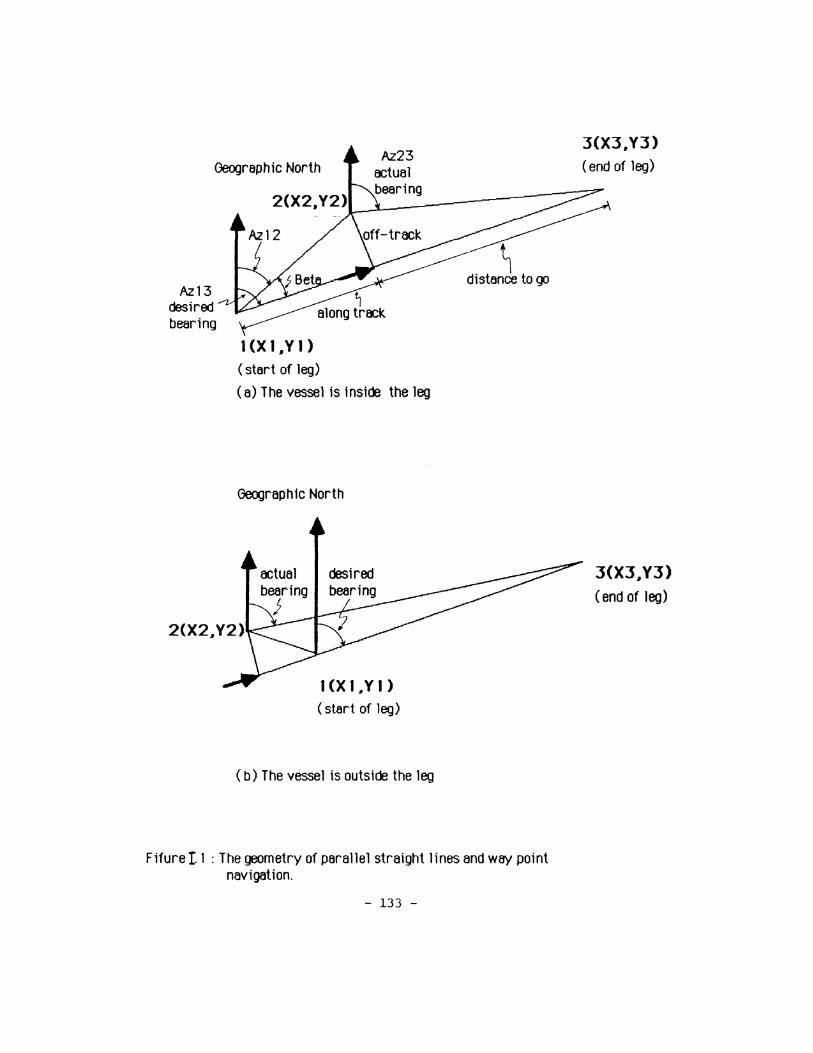
Geographic North
Az13 desired bearing
I(X l.Y 1)
(start of leg)
(a) The vessel is inside the leg
Geographic North
I(X 1 .. Y 1) (start of leg)
(b) The vessel is outside the leg
~ distance to go
Fifure I. 1 : The geometry of parallel straight lines and Wf!Y point navigation.
- 133 -
J(XJ.YJ) (end of leg)
3(X3.Y3) (end of leg)
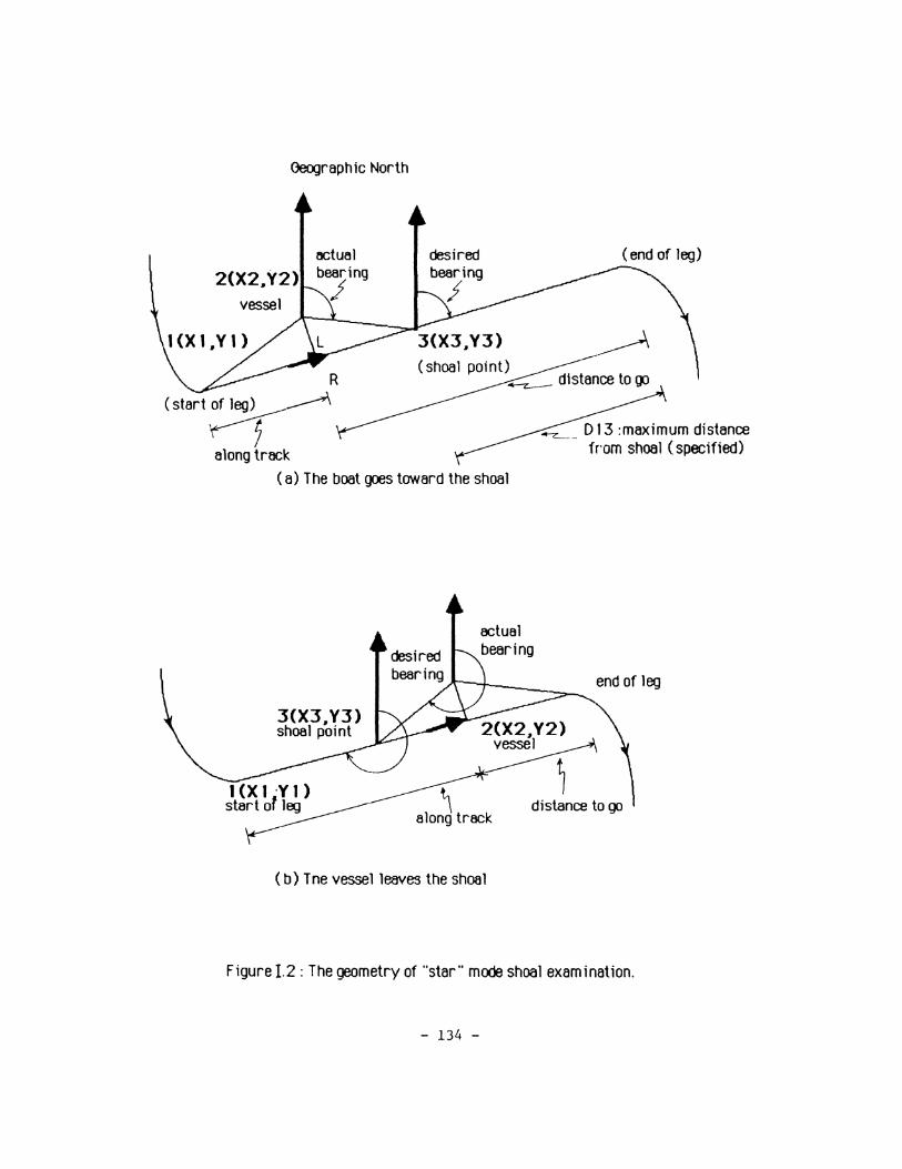
Oeographic North
R
(start~
(shoal point) -.:.-- distance to go
along track
(a) The boat goes toward the shoal
3(X3,Y3) shoal point
(b) Tne vessel leaves the shoal
....-z___ D 13 :maximum distance from shoal (specified)
Figure 1.2: The geometry of "star" mode shoal examination.
- 134 -
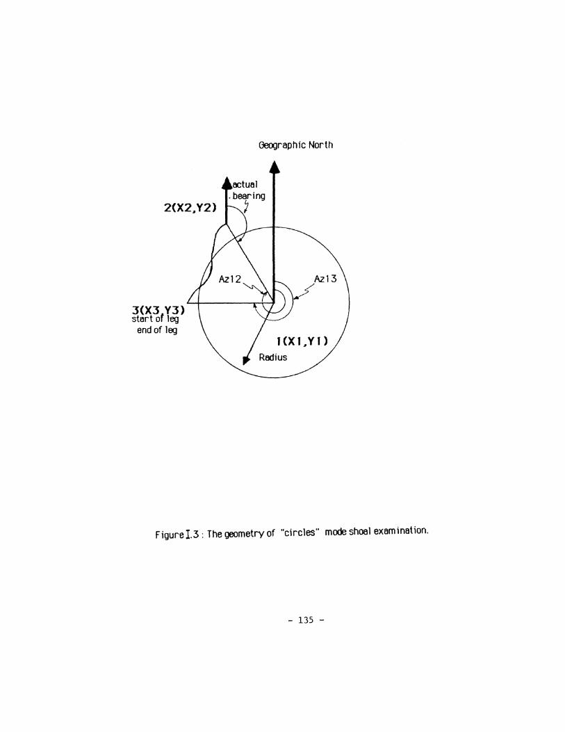
2(X2~Y2)
3(X3 Y3) start of leg
end of leg
Geo,;Jraphic North
Figurei.3: The geometry of "circles" mode shoal examination.
- 135 -