Physica D 340 (2017) 46–57

Contents lists available at ScienceDirect

Physica D

journal homepage: www.elsevier.com/locate/physd

Data-based stochastic model reduction for the Kuramoto–SivashinskyequationFei Lu a,b,⇤, Kevin K. Lin c, Alexandre J. Chorin a,b

a Department of Mathematics, University of California, Berkeley, United Statesb Lawrence Berkeley National Laboratory, United Statesc School of Mathematics, University of Arizona, United States

h i g h l i g h t s

• A discrete-time data-driven stochastic model reduction method for predictive modeling.• The reduced model captures large time behavior of a chaotic PDE.• A parametric implementation of approximate inertial manifold (AIM) methods.• A non-Markov model representing memory effect of unresolved variables.• A framework integrating numerical schemes and AIMs into statistical inference.

a r t i c l e i n f o

Article history:Received 1 October 2015Accepted 25 September 2016Available online 3 October 2016Communicated by E.S. Titi

Keywords:Stochastic parametrizationNARMAXKuramoto–Sivashinsky equationApproximate inertial manifold

a b s t r a c t

The problem of constructing data-based, predictive, reduced models for the Kuramoto–Sivashinskyequation is considered, under circumstances where one has observation data only for a small subsetof the dynamical variables. Accurate prediction is achieved by developing a discrete-time stochasticreduced system, based on a NARMAX (Nonlinear Autoregressive Moving Average with eXogenous input)representation. The practical issue, with the NARMAX representation as with any other, is to identifyan efficient structure, i.e., one with a small number of terms and coefficients. This is accomplished hereby estimating coefficients for an approximate inertial form. The broader significance of the results isdiscussed.

© 2016 Elsevier B.V. All rights reserved.

1. Introduction

There aremanyhigh-dimensional dynamical systems in scienceand engineering that are too complex or computationally expen-sive to solve in full, and where only a relatively small subset ofthe degrees of freedom are observable and of direct interest. Un-der these conditions, it is useful to derive low-dimensional modelsthat can predict the evolution of the variables of interest withoutreference to the remaining degrees of freedom, and reproduce theirstatistics at an acceptable cost.

We assume here that the variables of interest have been ob-served in the past, and we consider the problem of deriving low-dimensional models on the basis of such prior observations. We

⇤ Corresponding author at: Department of Mathematics, University of California,Berkeley, United States.

E-mail addresses: feilu@berkeley.edu (F. Lu), klin@math.arizona.edu (K.K. Lin),chorin@math.berkeley.edu (A.J. Chorin).

do the analysis in the case of the Kuramoto–Sivashinsky equation(KSE):

@v

@t+ v

@v

@x+ @2v

@x2+ @4v

@x4= 0 , x 2 R, t > 0; (1)

v(x, t) = v(x + L, t); v(x, 0) = g(x),

where t is time, x is space, v is the solution of the equation, L is anassumed spatial period, and g is the initial datum. We pick a smallinteger K , and assume that one can observe only the Fouriermodesof the solution with wave numbers k = 1, . . . , K at a discrete se-quence of points in time. To model the usual situation where theobserved modes are not sufficient to determine a solution of thedifferential equations without additional input, we pick K smallenough so that the dynamics of a Galerkin–Fourier representationof the solution, truncated so that it contains only K modes, arefar from the dynamics of the full system. The goal is to accountfor the effects of ‘‘model error’’, i.e. for the effects of the missing‘‘unresolved’’ modes on the ‘‘resolved’’ modes, by suitable terms in

http://dx.doi.org/10.1016/j.physd.2016.09.0070167-2789/© 2016 Elsevier B.V. All rights reserved.

F. Lu et al. / Physica D 340 (2017) 46–57 47

reduced equations for the resolved modes, using the informationcontained in the observations of the resolved modes; we are notinterested in the unresolved modes per se. In the present paperthe observations are obtained by a solution of the full system; wehope that our methods are applicable to problems where the datacome from physical measurements, including problems where afull model is not known.

We start from the truncated equations for the resolved modes,and solve an inverse problem where the data are used to estimatethe effects of model error, i.e., what needs to be added to thetruncated equations for the solution of the truncated equationsto agree with the data. Once these effects are estimated, theyneed to be identified, i.e., summarized by expressions that canbe readily used in computation. In our problem the addedterms can take a range of values for each value of the resolvedvariables, and therefore a stochastic model is a better choice thana deterministic model. We solve the inverse problem within adiscrete-time setting (see [1]), and then identify the needed termswithin aNARMAX (NonlinearAutoregressionwithMovingAverageand eXogenous input) representation of discrete time series.The determination of missing terms from data is often called a‘‘parametrization’’; what we are presenting is a discrete stochasticparametrization. Themain difficulty in stochastic parametrization,as in non-parametric statistical inference problems, is making theidentified representation efficient, i.e., with a small number ofterms and coefficients. We accomplish this by a semi-parametricapproach: we propose terms for the NARMAX representation froman approximate ‘‘inertial form’’ [2], i.e., a system of ordinarydifferential equations that describes the motion of the systemon a finite-dimensional, globally attracting manifold called an‘‘inertial manifold’’. (Relevant facts from inertial manifold theoryare reviewed later.)

A number of stochastic parametrization methods have beenproposed in recent years, often in the context of weather andclimate prediction. In [3–5], model error is represented as the sumof an approximating polynomial in the resolved variables, obtainedby regression, and a one-step autoregression. The shortcomingsof this representation as a general tool are that it does notallow the model error to depend sufficiently on the past valuesof the solution, that the model error is calculated inaccurately,especially when the data are sparse, and that the autoregressionterm is not necessarily small, making it difficult to solve theresulting stochastic equations accurately. Detailed comparisonsbetween this approach and a discrete-time NARMAX approachcan be found in [1]. In [6,7] the model error is represented asa conditional Markov chain that depends on both current andpast values of the solution; the Markov chain is deduced fromdata by binning and counting, assuming that exact observationsof the model error are available, i.e., that the inverse problemhas been solved perfectly. It should be noted that the Markovchain representation is intrinsically discrete, making this workclose to ours in spirit. In [8] the noise is treated as continuous andrepresented by a hypo-elliptic system that is partly analogous tothe NARMAX representation, once translated from the continuumto the grid. An earlier construction of a reduced approximation canbe found in [9], where the approach was not yet fully discrete.Other interesting relatedwork canbe found in [10–14]. Thepresentauthors’ previouswork on the discrete-time approach to stochasticparametrization and the use of NARMAX representations can befound in [1].

The KSE is a prototypical model of spatiotemporal chaos. As anonlinear PDE, it has features found in more complex models ofcontinuum mechanics, yet its analysis and numerical solution arefairly well understood because of its relatively simple structure.There is a lot of previous work on stochastic model reductionfor the KSE. Yakhot [15] developed a dynamic renormalization

group method for reducing the KSE, and showed that the modelerror generates a random force and a positive viscosity. Recentdevelopment of this method can be found in [16,17]. Toh [18]studied the statistical properties of the KSE, and constructed astatistical model to reproduce the energy spectrum. Rost andKrug [19] presented a model of interacting particles on the linewhich exhibits spatiotemporal chaos, and made a connection withthe stochastic Burgers equation and the KPZ equation.

Stinis [20] addressed the problem of reducing the KSE as anunder-resolved computation problem with missing initial data,and used the Mori–Zwanzig (MZ) formalism [21] in the finitememory approximation [22,23] to produce a reduced system thatcan make short-time predictions. Full-system solutions were usedto compute the conditional means used in the reduced system. Asdiscussed in [1], the NARMAX representation can be thought of asboth a generalization and an implementation of theMZ formalism,and the full-system solutions used by Stinis can be viewed as data,so that the pioneering work of Stinis is close in spirit to our work.We provide below a comparison of our work with that of Stinis.

The paper is organized as follows. In Section 2, we introduce theKuramoto–Sivashinsky equation, the dynamics of its solutions, andits numerical solution by spectral methods. In Section 3 we applythe discrete approach for the determination of reduced systems tothe KSE, and discuss the NARMAX representation of time series. InSection 4 we use an inertial form to determine the structure of aNARMAX representation for the KSE, and estimate its coefficients.Numerical results are presented in Section 5. Conclusions and thebroader significance of the work, as well as its limitations, arediscussed in a concluding section.

2. The Kuramoto–Sivashinsky equation

We begin with basic observations: in Eq. (1), the term @2v/@x2is responsible for instability at large scales, the dissipative term@4v/@x4 provides damping at small scales, and the non-linear termv@v/@x stabilizes the system by transferring energy between largeand small scales. To see this, first write the KSE in terms of Fouriermodes:

ddt

vk = (q2k � q4k)vk � iqk2

1X

l=�1vlvk�l, (2)

where the vk(t) are the Fourier coefficients

vk(t) := F [v(·, t)]k := 1L

Z L

0v(x, t)e�iqkxdx, (3)

where qk = 2⇡kL , k 2 Z, and F denotes the Fourier transform, so

that

v(x, t) = F �1[v·(t)] =+1X

k=�1vk(t)eiqkx. (4)

Since v is real, the Fourier modes satisfy v�k = v⇤k , where v⇤

k is thecomplex conjugate of vk. We refer to |vk(t)|2 as the ‘‘energy’’ of thekth mode at time t .

Next, we consider the linearization of the KSE about thezero solution. In the linearized equations, the Fourier modes areuncoupled, each represented by a first-order scalar ODE witheigenvalue q2k � q4k . Modes with |qk| > 1 are linearly stable;modes with |qk| 1 are not. The linearly unstable modes, ofwhich there are ⌫ = bL/2⇡c, are coupled to each other and tothe dampedmodes through the nonlinear term. Observe that if thenonlinear terms were not present, most initial conditions wouldlead to solutions whose energies blow up exponentially in time.The KSE is, however, well-posed (see, e.g., [24]), and it can beshown that solutions remain globally bounded in time (in suitable

48 F. Lu et al. / Physica D 340 (2017) 46–57

Fig. 1. Solutions of the KSE. Left: a sample solution of the KSE. Right: Mean energy h|vk|2i as a function of k/⌫, where ⌫ = L/2⇡ is the number of unstable modes, for anumber of different values of L.

function spaces) [25,26]. The solutions of Eq. (1) do not growexponentially because the quadratic nonlinearities,which formallyconserve the L2 norm, serve to transport energy from low to highmodes. Fig. 1 shows an example solution, as well as the energyspectrum h|vk|2i, where h�i denotes the limit of 1

T

R T0 �(v(t))dt as

T ! 1 . The energy spectrum has a characteristic ‘‘plateau’’ forsmall wave numbers, which gives way to rapid, exponential decayas k increases, see Fig. 1 (right). This concentration of energy inthe low-wavenumber modes is reflected in the cellular characterof the solution in Fig. 1 (left), where the length scale of the cells isdetermined by the modes carrying the most energy.

Another feature of the nonlinear energy transfer is that theKSE possesses an inertial manifold M . When the KSE is viewed asan infinite-dimensional dynamical system on a suitable functionspace B, there exists a finite-dimensional submanifold M ⇢ Bsuch that all solutions of the KSE tend asymptotically to M (seee.g. [24]). The long-time dynamics of the KSE are thus essentiallyfinite-dimensional. Moreover, it can be shown that for sufficientlylarge N (N > dim(M) at the very minimum), an inertial manifoldM can be written in the form

M = {x + (x)|x 2 ⇡N(B)}, (5)

where ⇡N is the projection onto the span of {eikx, k = 1, . . . ,N},and : ⇡N(B) ! (⇡N(B))? is a Lipschitz-continuous map.That is to say, for trajectories lying on the inertial manifold M ,the high-wavenumber modes are completely determined by thelow-wavenumber modes. Inertial manifolds will be useful inSection 4, and we say more about them there.

The KSE system is Galilean invariant; if v(x, t) is a solution, thenv(x � ct, t) + c , with c an arbitrary constant velocity, is also asolution. Without loss of generality, we set

Rv(x, 0)dx = 0, which

implies that v0(0) = 0. From (2), we see that v0(t) ⌘ 0 for all t andRv(x, t)dx ⌘ 0. In physical terms, solutions v(x, t) of the KSE can

be interpreted as the velocity of a propagating ‘‘front,’’ for exampleas in flame propagation, and this decoupling of the v0 equationfrom vk for k 6= 0 means the mean velocity is conserved.

Chaotic dynamics and statistical assumptions

Numerous studies have shown that the KSE exhibits chaoticdynamics, as characterized by a positive Lyapunov exponent,exponentially decaying time correlations, and other signatures ofchaos (see, e.g., [27] and references therein). Roughly speaking,this means that nearby trajectories tend to separate exponentiallyfast in time, and that, though the KSE is a deterministic equation,its solutions are unpredictable in the long run as small errors

in initial conditions are amplified. Chaos also means that astatistical modeling approach is natural. In what follows, weassume our system is in a chaotic regime, characterized by atranslation-invariant physical invariant probability measure (see,e.g., [28,29] for the notion of physical invariant measures andtheir connections to chaotic dynamics). That is, we assume thatnumerical solutions of the KSE, sampled at regular space and timeintervals, form (modulo transients) multidimensional time seriesthat are stationary in time and homogeneous in space, and thatthe resulting statistics are insensitive to the exact choice of initialconditions. Exceptwhere noted, this assumption is consistent withnumerical observations. Hereafter we will refer to this as ‘‘the’’ergodicity assumption, as this is the assumption of ergodicityneeded in the present paper.

The translation-invariance part of our ergodicity assumptionhas the consequence, the Fourier coefficients cannot have apreferred phase in steady state, i.e., the physical invariant measurehas the property that if we write the kth Fourier coefficient vk(see below) as akei✓k , then the ✓k are uniformly distributed. Thetheory of stationary stochastic processes also tells us that distinctFourier modes are uncorrelated [23], though they are generallynot independent: one can readily show this by, e.g., checking thatcov(|vk|2, |v`|2) 6= 0 numerically. (Such energy correlations areyet another consequence of the nonlinear term acting to transferenergy between modes.)

Numerical solution

For purposes of numerical approximation, the system canbe truncated as follows: the function v(x, t) is sampled at thegrid points xn = nL/N, n = 0, . . . ,N � 1, so that vN =(v(x0, t), . . . , v(xN�1, t)), where the superscript N in vN is areminder that the sampled v varies as N changes. The Fouriertransform F is replaced by the discrete Fourier transform FN(assuming N is even):

vNk = FN [v(·, t)]k =

N�1X

n=0

vN(xn, t)e�iqkxn ,

and

vN(xn, t) = F �1N [vN

· (t)] = 1N

N/2X

k=�N/2+1

vNk (t)eiqkxn .

Noting that vN0 = 0 due to Galilean invariance, and setting vN

N/2 =0, we obtain a truncated systemddt

vNk = (q2k � q4k)v

Nk � iqk

2

X

1|l|N,1|k�l|N

vNl vN

k�l, (6)

F. Lu et al. / Physica D 340 (2017) 46–57 49

with k = �N/2 + 1, . . . ,N/2. This is a system of ODE (of thereal and imaginary parts of vN

k ) in RN�2, since vN�k = vN,⇤

k andvNN/2 = vN

0 ⌘ 0.Fourier modes with large wave numbers are typically small

and can be neglected, as can be seen from a linear analysis: vk

decreases at approximately the rate e(q2k�q4k )t , where qk = kL/2⇡(see Fig. 1 (right)). A truncation with N � 8⌫ = 8bL/2⇡c canbe considered accurate. In the following, a truncated system withN = 32⌫ = 32bL/2⇡c is considered to be the ‘‘full’’ system, andwe aim to construct reduced models for K < 2⌫ ⇡ L/⇡ . Exceptwhen N is small, the system (6) is stiff (since qk grows rapidlywith k). To handle this stiffness and maintain reasonable accuracy,we generate data by solving the truncated KSE by an exponentialtime difference fourth order Runge–Kutta method (ETDRK4)[30,31] with standard 3/2 de-aliasing (see, e.g., [32,33]). Wesolve the full system with a small step size dt , and then makeobservations of the modes with wave numbers k = 1, . . . , K ata times separated by a larger time interval � > dt , and denote theobserved data by

{vk(tn), k = 1, . . . , K , n = 0, . . . , T } ,

where tn = n�.To predict the evolution of K observed modes with wave

numbers k = 1, . . . , K , it is natural to start from the truncatedsystem that includes only these modes, i.e., the system (6) withN = 2(K + 1). However, when one takes K to be relatively small(as we do in the present paper), large truncation errors are present,and the dynamics of the truncated system are very different fromthose of the full system.

3. A discrete-time approach to stochastic parametrization and

the NARMAX representation

Suppose one is given a dynamical system

d�dt

= F(�), (7)

where the variables are partitioned as � = (u, w), with urepresenting a (possibly quite small) subset of variables of directinterest. The problem of model reduction is to develop a reduceddynamical system for predicting the evolution of u alone. That is,one wishes to find an equation for u that has the form

dudt

= R(u) + z(t), (8)

where R(u) is a function of u only, and z(t) represents the modelerror, i.e., the quantity one should add to R(u) to obtain the correctevolution. For example, if � represents the full state (vk, k 2Z) of a KSE solution and u represents the low-wavenumbermodes (v�K , v�K+1, . . . , vK ), then R can correspond to a K -modetruncation of the KSE. In general, the model error z must dependon u, since the resolved variables u and unresolved variables wtypically interact.

The usual approach to stochastic parametrization and modelreduction as formulated above is to identify z as a stochasticprocess in the differential equation (8) from data (see [3,4,6,8]and references therein). This approach has major difficulties. First,it leads to the challenging problem of statistical inference for acontinuous-time nonlinear stochastic system from partial discreteobservations [34,35]. The data are measurements of u, not ofz; to find values of z one has to use Eq. (8) and differentiatex numerically, which may be inaccurate because z may havehigh-frequency components or fail to be sufficiently smooth, andbecause the data may not be available at sufficiently small timeintervals. Then, if one can successfully estimate values of z and

then identify it, Eq. (8) becomes a nonlinear stochastic differentialsystem, which may be hard to solve with sufficient accuracy (seee.g [36,37]).

To avoid these difficulties, a purely discrete-time approach tostochastic parametrization was proposed in [1]. This approachavoids the difficult detour through a continuous-time stochasticsystem followed by its discretization, by working entirely in adiscrete-time setting. It starts from the truncated equationdydt

= R(y).

(y differs from u in that its evolution equation is missing theinformation represented by the model error z(t) in Eq. (8), andso is not up to the task of computing u.) Fix a step size � > 0,and choose a method of time-discretization, for example fourth-order Runge–Kutta. Then discretize the truncated equation aboveto obtain a discrete-time approximation of the form

yn+1 = yn + �R�(yn).

(The function R� depends on the numerical time-stepping schemeused.) To estimate the model error, write a discrete analog ofEq. (8):

un+1 = un + �R�(un) + �zn+1. (9)

Note that a sequence of values of zn+1 can be computed from datausing

zn+1 = un+1 � un

�� R�(un), (10)

where the values of u are the observed values; the resulting valuesof z account for both themodel error in (8) and the numerical errorin the discretization R�(un). The task at hand is to identify the timeseries {zn} as a discrete stochastic process which depends on u.Once this is done, Eq. (9) will be used to predict the evolution ofu. There is no need to approximate or differentiate, and there is nostochastic differential equations to solve. Note that the zn dependon the numerical error as well as on the model error, and maynot be good representations of the continuummodel error; we arenot interested in the latter, we are only interested in modeling thesolution u.

The sequence {zn} is a stationary time series, which we rep-resent via a NARMAX representation, with u as an exogenous in-put. This representation makes it possible to take into accountefficiently the non-Markovian features of the reduced system aswell asmodel andnumerical errors. TheNARMAX representation isversatile, easy to implement and reliable. The model inferred fromdata is exactly the same as the one used for prediction, which isnot the case for a continuous-time system because of numericalapproximations. The disadvantage of the discrete approach is thatthe discrete system depends on both the spacing of the observeddata and the method of time-discretization, so that data sets withdifferent spacing lead to different discrete systems.

The NARMAX representation has the form:

un+1 = un + �R�(un) + �zn+1,

zn = �n + ⇠ n, (11)

for n = 1, 2, . . ., where {⇠ n} is a sequence of independentidentically distributed random variables, the first equation repeatsEq. (9), and�n is a functional of current and past values of (u, z, ⇠),of the parametrized form:

�n = µ +pX

j=1

Ajzn�j +rX

j=1

BjQj(un�j) +qX

j=1

Cj⇠n�j, (12)

where�Qj, i = 1, . . . , r

�are functions to be chosen appropriately

and�µ, Aj, Bj, Cj

�are constant parameters to be inferred from

50 F. Lu et al. / Physica D 340 (2017) 46–57

data. Here we assume that the real and complex parts of ⇠ n areindependent and have Gaussian distributions with mean zero anddiagonal covariance matrix � 2.

We call the above equations a NARMAX representation becausethe time series {zn} in Eqs. (11)–(12) resemble the nonlinearautoregression moving average with exogenous input (NARMAX)model in e.g., [38–40]. In (12), the terms in z are the autoregressionpart of order p, the terms in ⇠ are the moving average part oforder q, and the terms Qj which depend on u are the exogenousinput terms. One should note that our representation is not quitea NARMAXmodel in the usual sense, because the exogenous inputin NARMAX is supposed to be independent of the output z, whilehere it is not. The system (11)–(12) is a nonlinear autoregressionmoving average (NARMA) representation of the time series {un}:by substituting (10) into (12) we obtain a closed system for u:

un+1 = un + �R�(un) + � n + �⇠ n+1, (13)

where n is a functional of the past values of u and ⇠ .The form of the system (11)–(12) is quite general. �n can be

a more general nonlinear functional of the past values of (u, z, ⇠)than the one in (12). The additive noise ⇠ can be replaced bya multiplicative noise. We leave these further generalizationsto future work. The main task in identification of a NARMAXrepresentation is to determine the structure of the functional �n,that is, determine the terms that are needed, then determine theorders (p, r, q) in (12) and estimate the parameters.

4. Determination of the NARMAX representation

To apply NARMAX to the KSE, one must first decide on thestructure of the model for zn. In particular, one must decide whichnonlinear terms to include in the ansatz. We note that a priori,it is clear that some nonlinear terms are necessary, as a simplelinear ansatz is very unlikely to be able to capture the dynamicsof the KSE. This is because distinct modes are uncorrelated (seeSection 2), so that if the ansatz for zn contains only linear terms,then the different components of our stochasticmodel for zn wouldbe independent, and onewould not expect such amodel to capturethe energy balance between the unresolved modes (see e.g. [8]).

But the question remains: which nonlinear terms? One optionis to include all nonlinear terms up to some order. This leads toa difficult parameter estimation problems because of the largenumbers of parameters involved. Moreover, a model with manyterms is likely to overfit, which complicates the model and leadsto poor predictive performance (see e.g. [38]). What we do hereinstead is use inertial manifolds as a guide to selecting suitablenonlinear terms. We note that our construction satisfies thephysical realizability constraints discussed in [8].

4.1. Approximate inertial manifolds

We begin with a quick review of approximate inertialmanifolds, following [2]. Write the KSE (1) in the formdvdt

= Av + f (v), v(x, 0) = g(x) 2 H,

where the linear operator A is the fourth derivative operator�@4/@x4 or, in Fourier variables, the infinite-dimensional di-agonal matrix with entries �q4k in (2), and where f (v) =�v@v/@x � @2v/@x2 or its spectral analog, and where H =�v 2 L2[0, L]|v(x) = v(x + L), x 2 R

. An inertial manifold is a

positively-invariant finite-dimensional manifold that attracts alltrajectories exponentially; see e.g. [24,41] for its existence, and seee.g. [42,43] for estimates of its dimension. It can be shown that in-ertial manifolds for the KSE are realizable as graphs of functions

: PH ! QH , where P is a suitable finite-dimensional projection(see below), and Q = I � P . The inertial form (the ordinary dif-ferential equation that describes motion restricted to the inertialmanifold) can be expressed in terms of the projected variable u by

dudt

= PAu + Pf (u + (u)), (14)

where u = Pv. Different methods for the approximation ofinertial manifolds have been proposed [2,44,45]. These methodsapproximate the function w = (u) by approximating theprojected system on QH ,

dwdt

= QAw + Qf (u + w), w(0) = Qg. (15)

In practice, P is typically taken to be the projection onto the span ofthe first m eigenfunctions of A, for example, one can set u = Pv =(v�m, v�m+1, . . . , vm), the first 2m Fourier modes. The dimensionof the inertial manifold is generally not known a priori [43], som is usually taken to be a large integer. It is shown in [46] thatfor large enough m and for v = u + w on the inertial manifold,dw/dt is relatively small. Neglecting dw/dt in (15) we obtain anapproximate equation for w:

w = �A�1Qf (u + w). (16)

Approximations of can then be obtained by setting up fixed pointiterations,

0 = 0, n+1 = �A�1Qf (u + n), (17)

and stopping at a particular finite value of n, which yields an ‘‘ap-proximate inertial manifold’’ (AIM). The accuracy of AIM improvesas its dimension m increases, in the sense that the distance be-tween the AIM and the global attractor of the KSE decreases at therate |qm|�� for some � > 0 [2].

In the application to our reduced KSE equation, one may try toset m = K . However, our cutoff K < 2⌫ ⇡ L

⇡is too small for there

to be a well-defined inertial form, since this is relatively close tothe number ⌫ = bL/2⇡c of linearly unstable modes, and we gen-erally expect any inertial manifold to have dimension much largethan 2⌫. Nevertheless, we will see that the above procedure forconstructing AIMs provides a useful guide for selecting nonlinearterms for NARMAX. This is unsurprising, since inertial manifoldsarise from the nonlinear energy transfer between low and highmodes and the strong dissipation at high modes, which is exactlywhat we hope to capture.

4.2. Structure selection

We now determine the structure of the NARMAX model,i.e., decide what terms should appear in (12). These terms shouldcorrectly reflect how z depends on u and ⇠ . Once the terms aredetermined, parameter estimation is relatively easy, as we see inthe next subsection. The number of terms should be as small aspossible, to save computing effort and to reduce the statistical errorin the estimate of the coefficients. One could try to determine theterms to be kept by looking for the terms that contribute mostto the output variance, see [38, Chapter 3] and the referencesthere. This approach fails to identify the right terms for stronglynonlinear systems such as the one we have. Other ideas based on apurely statistical approach have been explored e.g. in [38, Chapter9]. In the present paper, we design the nonlinear terms in (12)in the NARMAX model, which represents the model error in theK -mode truncation of the KSE, using the theory of inertialmanifolds sketched above.

In our setting, u = (v�K , . . . , vK ). Because of the quadraticnonlinearity, only the modes with wave number |k| = K + 1, K +

F. Lu et al. / Physica D 340 (2017) 46–57 51

2, . . . , 2K interact directlywith the observedmodes in u; henceweset w = (v�2K , . . . , v�K�1, vK+1, . . . , v2K ) in Eq. (16). Using theresult of a one-step iteration 1 = �A�1Qf (u) in (17) we obtainan expression for the high mode vk as a function of the low modesu:

1,k = � �A�1Qf (u)�k = � i

2q�4k

X

1|l|K ,1|k�l|K

vlvk�l,

for |k| = K + 1, K + 2, . . . , 2K .Our goal is to approximate the model error of the K -mode

Galerkin truncation, Pf (u + (u)) � Pf (u), so that the reducedmodel is closer to the attractor than the Galerkin truncation. Instandard approximate inertial manifold methods, the model erroris approximated by Pf (u + 1(u)) � Pf (u). Since K is relativelysmall in our setting, we do not expect the AIM approximationto be effective. However, in stochastic parametrization, we onlyneed a parametric representation of the model error, and morespecifically, to derive the nonlinear terms in the NARMAX model.As the AIM procedure implicitly takes into account energy transferbetween Fourier modes due to nonlinear interactions as well asthe strong dissipation in high modes, it can be used to suggestnonlinear terms to include in our NARMAX model. That is, theabove expressions of 1, Pf (u + 1(u)) � Pf (u) provide explicitnonlinear terms {�1,k�1,l,�1,kvj} we need (with K < |k|, |l| 2K , |j| K ); we simply leave the coefficients of these terms asfree parameters to be determined from data. Roughly speaking,the NARMAX can be viewed as a regression implementation of aparametric version of AIM.

Implementing the above observations in discrete time, we ob-tain the following terms to be used in the discrete reduced system:

eunj =

8><

>:

unj , 1 j K ;

iKX

l=j�K

unl u

nj�l, K < j 2K .

(18)

Themodes with negative wave numbers are defined byeun�j =eun,⇤

j .This yields the discrete stochastic system

un+1k = un

k + �R�k(un) + �zn+1

k ,

znk = �nk + ⇠ nk ,

where the functional�nk has the form:

�nk (✓k) = µk +

pX

j=1

ak,jzn�jk +

rX

j=0

bk,jun�jk +

KX

j=1

ck,jeunj+Keu

nj+K�k

+ ck,(K+1)R�k(un) +

qX

j=1

dk,j⇠n�jk , (19)

for 1 k K . Here ✓k = �µk, ak,j, bk,j, ck,j, dk,j

�are real parame-

ters to be estimated from data. Note that each one of the randomvariables ⇠ nk affects directly only onemode un

k , as is consistent withthe vanishing of correlations between distinct Fourier modes (seeSection 2).

We set �n�k = �

n,⇤k so that the solution of the stochastic

reduced system satisfies un�j = un,⇤

j . We include the terms inR�k(u

n) because theway theywere introduced in the above reducedstochastic system does not guarantee that they have the optimalcoefficients for the representation of z; the inclusion of these termsin �n

k makes it possible to optimize these coefficients. This issimilar in spirit to the construction of consistent reduced modelsin [13], though simpler to implement.

4.3. Parameter estimation

Weassume in this section that the terms and the orders (p, r, q)in the NARMAX representation have been selected, and estimatethe parameters as follows. To start, assume that the reducedsystem has dimension K , that is, the variables un, zn, �n and ⇠ nhave K components. Denote by ✓k = (µk, Ak,j, Bk,j, Ck,j) the set ofparameters in the kth component of�n, and ✓ = (✓1, ✓2, . . . , ✓K ) .We write�n

k as�nk (✓k) to emphasize that� depends on ✓k.

Recall that the real and complex parts of the components of⇠ n are independent N(0, � 2

k ) random variables. Then, following(11), the log-likelihood of the observations {un, q + 1 n N}conditioned on {⇠ 1, . . . , ⇠ q} is (up to a constant)

l(✓ , � 2|⇠ 1, . . . , ⇠ q)

= �KX

k=1

NX

n=q+1

��znk � �nk (✓)

��2

2� 2k

+ (N � q) ln � 2k

!

. (20)

If q = 0, this is the standard likelihood of the data {un, 1 n N},and the values of zn and �n(✓) can be computed from the data un

using (10) and (19), respectively. However, if q > 0, the sequence{�n

k (✓)} cannot be computed directly from data, due to itsdependence on the noise sequence {⇠ n}, which is unknown. Notethat once the values of {⇠ 1, . . . , ⇠ q} are available, one can computerecursively the sequence {�n

k (✓)} for n � q + 1 from data. Hencewe can compute the likelihood of {un, q + 1 n N} conditionalon {⇠ 1, . . . , ⇠ q}. If the stochastic reduced system is ergodic and thedata come from this system, the MLE is asymptotically consistent(see e.g. [47,39]), and hence the values of ⇠ 1, . . . , ⇠ q do not affectthe result if the data set is long enough. In practice, we can simplyset ⇠ 1 = · · · = ⇠ q = 0, the mean of these variables.

Taking partial derivatives with respect to � 2k and noting that��znk � �n

k (✓k)�� is independent of � 2

k , we find that the maximumlikelihood estimators (MLE) ✓ , � 2 satisfy the following equations:

✓k = argmin✓k

Sk(✓k), � 2k = 1

2(N � q)S(✓k), (21)

where

Sk(✓k) :=NX

n=q+1

��znk � �nk (✓k)

��2 .

Note first that in the case q = 0, the MLE ✓k follows directlyfrom least squares, because �n

k is linear in the parameter ✓k andits terms can be computed from data. If q > 0, the MLE ✓k canbe computed either by an optimizationmethod (e.g. quasi-Newtonmethod), or by iterative least squares method (see e.g. [48]). Witheithermethod, one first computes�n

k (✓k)with the current value ofparameter ✓k, and then one updates ✓k (by gradient searchmethodsor by least squares), and repeats until the error tolerance forconvergence is reached. The starting values of ✓k for the iterationsfor either method are set to be the least square estimates using theresidual of the corresponding q = 0 model.

The simple forms of the log-likelihood in (20) and the MLEsin (21) are based on the assumption that the real and complexparts of the components of ⇠ n are independent Gaussians. Onemay allow the components of ⇠ n to be correlated, at the cost ofintroducingmore parameters to be estimated. Also, similar to [48],this algorithm can be implemented online, i.e. recursively as thedata size increases, and the noise sequence {⇠ n} can be allowed tobe non-Gaussian (on the basis of martingale arguments).

52 F. Lu et al. / Physica D 340 (2017) 46–57

4.4. Order selection

In analogy to the earlier discussion, it is not advantageous tohave large orders (p, r, q) [38,49], because, while large ordersgenerally yield small noise variance, the errors arising fromthe estimation of the parameters accumulate as the number ofparameters increases. The forecasting ability of the reduced modeldepends not only on the noise variance but also on the errors inparameter estimation. For this reason, a penalty factor is oftenintroduced discourage the fitting of linear models with too manyparameters. Many criteria have been proposed for linear ARMAmodels (see e.g. [49]). However, due to the nonlinearity of NARMAand NARMAX models, these criteria do not work for them.

Here we propose a number of practical, qualitative criteria forselecting orders by trial and error. We first select orders, estimatethe parameters for these orders, and then analyze how well theestimated parameters and the resulting reduced system reach ourgoals. The criteria are:

1. The variance of the model error should be small.2. The stochastic reduced system should be stable, and its long-

term statistical properties should be well-defined (i.e., thereduced system should have a stationary distribution), andshould agree with the data. Especially, the autocorrelationfunctions (which are computed by time averaging) of thereduced system and of the data should be close.

3. The estimated parameters should converge as the size of thedata set increases.

These criteria do not necessarily produce optimal solutions. Asin most statistics problems, one is aiming at an adequate ratherthan a perfect solution.

5. Numerical results

5.1. Estimated NARMAX coefficients

We now determine the coefficients and the orders in thefunctional � of Eq. (12) in the case L = 2⇡/

p0.085, K = 5;

for this choice of L, the number of linearly unstable modes is ⌫ =b1/p0.085c = 3. This setting is the same as in Stinis [20], up to achange of variables in the solution. We obtain data by solving thefull Eq. (6) with N = 32bL/2⇡c and with time step dt = 0.001,and make observations of the first K modes with wave numberk = 1, . . . , K , with time spacing � = 0.1. As initial value wetake v0(x) = (1 + sin x) cos x. Recall that we denote by {v(tn)}Tn=1the observations of the K modes. We choose the length of the dataset to be large enough so that the statistics can be computed bytime averaging. The means and variances of the real parts of theobserved Fouriermodes settle down after about 5⇥104 time units.Hence we drop the first 104 time units, and use observations of thenext 5 ⇥ 104 time units as data for inferring a reduced stochasticsystem; with (estimated) integrated autocorrelation times of theFourier modes ranging from ⇡10 to ⇡35 time units, this amountof data should be sufficient for estimating the coefficients. (Because� = 0.1, the length of data is T = 5 ⇥ 105.)

We consider different orders (p, r, q): p = 0, 1, 2; r =1, 2; q = 0, 1. We first estimate the parameters by the conditionallikelihood method described in Section 4.3. Then we numericallytest the stability of the stochastic reduced system by generating along trajectory of length T , starting from an arbitrary point in thedata (for example v(t20000)). We then drop the orders that lead tounstable systems, and select, among the remaining orders, the oneswith smallest noise variances.

The orders (2, 1, 0), (2, 2, 0) lead to unstable reduced system,though their noise variances are the smallest, see Table 1. Thissuggests that large orders p, r, q are not needed. Among the other

Table 1

The noise variances in the NARMAX with different orders (p, r, q).

(p, r, q) scale � 21 � 2

2 � 23 � 2

4 � 25

010 ⇥10�3 0.0005 0.0061 0.0217 0.1293 0.1638020 ⇥10�3 0.0005 0.0051 0.0187 0.0968 0.1612110 ⇥10�4 0.0047 0.0587 0.1664 0.4290 0.5640120 ⇥10�4 0.0044 0.0509 0.1647 0.4148 0.3259021 ⇥10�4 0.0012 0.0129 0.0472 0.2434 0.4056111 ⇥10�4 0.0012 0.0148 0.0421 0.1079 0.1426210 ⇥10�5 0.0020 0.0307 0.1533 0.3921 0.3234220 ⇥10�5 0.0019 0.0304 0.1450 0.2858 0.1419

Table 2

The average of mean square distances between the autocorrelation functions of thedata and the autocorrelation functions NARMAX trajectory with different orders(p, r, q).

(p, r, q) D1 D2 D3 D4 D5

020 0.0012 0.0013 0.0008 0.0004 0.0009021 0.0010 0.0010 0.0007 0.0004 0.0008111 0.0013 0.0019 0.0010 0.0004 0.0010110 0.0011 0.0018 0.0008 0.0005 0.0010120 0.0013 0.0022 0.0010 0.0004 0.0011

orders, the choices (0, 2, 1) and (1, 1, 1) have the smallest noisevariances (see Table 1). The orders (1, 1, 1) seems to be betterthan (0, 2, 1), because the former has four out of the five variancessmaller than the latter.

For further selection, following the second criterion in Sec-tion 4.4, we compare the empirical autocorrelation functionsof the NARMAX reduced system with the autocorrelation func-tions of data. Specifically, first we take N0 pieces of the data,{(v(tn), n = ni, ni + 1, . . . , ni + T )}N0

i=1 with ni+1 = ni + Tlag/�,where T is the length of each piece and Tlag is the time gap betweentwo adjacent pieces. For each piece (v(tn), n = ni, . . . , ni + T ), wegenerate a sample trajectory of length T from the NARMAX re-duced system using initial

�v(tni), v(tni+1), . . . , v(tni+m)

�, where

m = max {p, r, 2q} + 1, and denote the sample trajectory by�uni+n, n = 1, . . . , T

�. Here an initial segment is used to estimate

the first few steps of the noise sequence,�⇠ q+1, . . . , ⇠ 2q

�(recall

that we set ⇠ 1 = · · · = ⇠ q = 0). Then we compute the auto-correlation functions of real parts each trajectory by

�v,k(h, i) = 1T � h

T�hX

n=1

Re vk(tni+n+h) Re vk(tni+n);

�u,k(h, i) = 1T � h

T�hX

n=1

Re uni+n+hk Re uni+n

k ,

for h = 1, . . . , Tlag/�, i = 1, . . . ,N0, k = 1, . . . , K , and computethe average of mean square distances between the autocorrelationfunctions by

Dk = 1N0

N0X

i=1

�

Tlag

Tlag/�X

h=1

���v,k(h, i) � �u,k(h, i)��2!

.

The orders (p, r, q) with the smallest average mean square dis-tances will be selected. Here we only consider the autocorrelationfunctions of the real parts, since the imaginary parts have statisticalproperties similar to those of the real parts.

Table 2 shows the average of mean square distances betweenthe autocorrelation functions for different orders and the autocor-relation functions of the data, computedwithN0 = 100, Tlag = 50.The orders (1, 1, 1) have larger distances than (0, 2, 1). We selectthe orders (0, 2, 1) because they have the smallest average ofmeansquare distances. The estimated parameters for the orders (0, 2, 1)are presented in Table 3.

F. Lu et al. / Physica D 340 (2017) 46–57 53

Table 3

The estimated parameters in the NARMAX with orders (p, r, q) = (0, 2, 1).

k µk(⇥10�4) bk,0 bk,1 dk,1 � 2k (⇥10�4)

1 0.0425 0.0909 �0.0910 0.9959 0.00122 �0.0073 0.1593 �0.1600 0.9962 0.01383 0.3969 0.2598 �0.2617 0.9942 0.05204 �0.9689 0.7374 �0.7408 0.9977 0.25445 �0.1674 0.3822 �0.3799 0.9974 0.4056

k ck,1 ck,2(⇥10�3) ck,3(⇥10�3) ck,4(⇥10�3) ck,5(⇥10�3) ck,61 0.0002 0.0000 0.0010 0.0013 �0.0003 �0.00822 0.0005 0.2089 0.0015 0.0007 0.0001 �0.01573 0.0008 0.3836 0.1055 �0.0013 �0.0040 �0.02834 0.0010 0.5841 0.2971 �0.4104 0.0449 �0.08005 0.0012 0.6674 0.4763 0.2707 0.1016 �0.0710

(a) The truncated system. (b) NARMAX.

Fig. 2. Semilog plot of the probability density functions reproduced by the truncated system and by the NARMAX system (red ⇥’s), compared to the full system (blue dots).Here we only plot the real parts of the paths of the Fourier modes (from top to bottom, the wave numbers are k = 1, 2, . . . , 5). Note the distributions of the truncated systemare not symmetric because solutions appear to converge to a fixed point, so that our ergodicity assumption is invalid. (For interpretation of the references to color in thisfigure legend, the reader is referred to the web version of this article.)

For comparison, we also carried out a similar analysis for � =0.01. We found (data not shown) that (i) the best choices of(p, r, q) are different for � = 0.1 and for � = 0.01; and (ii) thecoefficients do not scale in a simple way, e.g., all as some power of�. Presumably, there is an asymptotic regime (as � ! 0) in whichthe coefficients do exhibit some scaling, but � = 0.1 is too largeto exhibit any readily-discernible scaling behavior. We leave theinvestigation of the scaling limit as � ! 0 for future work.

We observed that for all the above orders,most of the estimatedparameters show a clear trend of convergence as the length ofthe data set increases, but some parameters keep oscillating (datanot shown). For example, for NARMAX with orders (0, 2, 1), thecoefficients bk,j are more oscillatory than the coefficients ck,j, andthe parameters of the mode with wave number k = 5 are moreoscillatory than the parameters of other modes. This indicatesthat the structure and the orders are not yet optimal, and weleave the task of developing better structures and orders to futurework. Here we select the orders simply based on the size ofnoise variances and on the ability to reproduce the autocorrelationfunctions. Yetwe obtain a reduced systemwhich achieves both our

goals of reproducing the long-term statistics and making reliableshort-term forecasting, as we show in the following sections.

In the following, we select the orders (0, 2, 1) for the NARMAXreduced system.

5.2. Long-term statistics

We compare the statistics of the truncated system and theNARMAX reduced system with the statistics of the data. Wecalculate the following quantities for the reduced systems aswell as for data: the empirical probability density functions (pdf)and the empirical autocorrelation functions for each of the Kcomponents. All these statistics are computed by time-averaginglong sample trajectories, as we did for the autocorrelationfunctions in the previous subsection.

The pdfs and autocorrelation functions of data are reproducedwell by the NARMAX reduced system, as shown in Figs. 2 and 3.The NARMAX system reproduces almost exactly the pdfs and theautocorrelation functions of the data, a significant improvementover the truncated system.

54 F. Lu et al. / Physica D 340 (2017) 46–57

(a) The truncated system. (b) NARMAX.

Fig. 3. The autocorrelation functions reproduced by the truncated system and the NARMAX system (dot–dash line), compared to the full system (solid line). Here we onlyplot the real parts of the paths of the Fourier modes (from top to bottom, the wave numbers are k = 1, 2, . . . , 5).

We also computed energy covariances cov(|vk|2, |v2` |) for some

pairs (k, `) with k 6= `. (Recall from Section 2 that this is expectedto be nonzero.) In particular, testswith k = 2 and ` 2 {1, 2, 3, 4, 5}show that the NARMAX reduced system can correctly capturethese energy–energy covariances, whereas the truncated systemdoes not (data not shown).

5.3. Short-term forecasting

We now investigate how well the NARMAX reduced systempredicts the behavior of the full system.

We start from single path forecasts. For the NARMAX withorders (p, r, q), we start the multistep recursion by using an initialsegment with m = 2max{p, r, q} + 1 steps as follows. We set⇠ 1 = · · · = ⇠ q = 0, and estimate ⇠ q+1, . . . , ⇠m using Eq. (11).Then we follow the discrete system to generate an ensembleof trajectories from different realizations, with all realizationsusing the same initial condition. We do not introduce artificialperturbations into the initial conditions, because the exact initialconditions are known. A typical ensemble of 20 trajectories, aswellas its mean trajectory and the corresponding data trajectory, isshown in Fig. 4(b). As a comparison, we also plot a forecast usingthe truncated system. Since the observations provide the exactinitial condition, the truncated system produces a single forecastpath, see Fig. 4(a). We observe that the ensemble of NARMAXfollows the true trajectory well for about 50 time units, and thespread becomes wide quickly afterwards, while the ensemblemean can follow the true trajectory to 55 time units. Compared tothe truncated system which can make forecast for about 20 timeunits, NARMAX canmake forecast for about 55 time units, which isa significant improvement. We comment that the prediction timein [20], in which used the Mori–Zwanzig formalism, was about 35time units.

To measure the reliability of the forecast as a function of leadtime, we compute two commonly-used statistics, the root-mean-square-error (RMSE) and the anomaly correlation (ANCR). Both

statistics are based on generating a large number of ensembles oftrajectories of the reduced system starting from different initialconditions, and comparing the mean ensemble predictions withthe true trajectories, as follows.

First we take N0 short pieces of the data, {(v(tn), n = ni, ni

+1, . . . , ni+T )}N0i=1 with ni+1 = ni+Tlag/�, where T = Tlag/� is the

length of each piece and Tlag is the time gap between two adjacentpieces. For each short piece of data (v(tn), n = ni, . . . , ni + T ), wegenerate Nens trajectories of length T from the NARMAX reducedsystem, starting all ensemble members from the same several-step initial condition

�v(tni), v(tni+1), . . . , v(tni+m)

�, where m =

2max {p, r, q} + 1, and denote the sample trajectories by(un(i, j), n = 1, . . . , T ) for i = 1, . . . ,N0 and j = 1, . . . ,Nens.Again, we do not introduce artificial perturbations into the initialconditions, because the exact initial conditions are known, and byinitializing from data, we preserve the memory of the system so asto generate better ensemble trajectories.

We then calculate the mean trajectory for each ensemble,un(i) = 1

Nens

PNensj=1 un(i, j). The RMSE measures, in an average

sense, the difference between the mean ensemble trajectory,i.e., the expected path predicted by the reducedmodel, and the truedata trajectory:

RMSE(⌧n) :=

1N0

N0X

i=1

��Re v(tni+n) � Re un(i)��2!1/2

,

where ⌧n = n�. The anomaly correlation (ANCR) shows the averagecorrelation between the mean ensemble trajectory and the truedata trajectory (see e.g. [6]):

ANCR(⌧n) := 1N0

N0X

i=1

a

v,i(n) · au,i(n)q

|av,i(n)|2 ��au,i(n)��2,

where av,i(n) = Re v(tni+n)�Re hvi and a

u,i(n) = Re un(i)�Re hviare the anomalies in data and the ensemble mean. Here a · b =

F. Lu et al. / Physica D 340 (2017) 46–57 55

(a) The truncated system. (b) NARMAX.

Fig. 4. A typical path forecast made by the reduced systems compared to the data (solid line). (a) the truncated system (dot–dashed line); (b) ensemble trajectories (cyanline) and the mean trajectory of the ensemble (dot–dashed line) of the NARMAX system. Here we only plot the real parts of the paths of the Fourier modes (from top tobottom, the wave numbers are k = 1, . . . , 5). (For interpretation of the references to color in this figure legend, the reader is referred to the web version of this article.)

(a) RMSE. (b) ANCR.

Fig. 5. Root-mean-square-error (RMSE) and Anomaly correlations (ANCR) of ensemble forecasting, produced by the NARMAX system (solid lines) and the truncated system(dot–dashed line), for different ensemble sizes: Nens = 1 (circle marker), Nens = 5 (cross marker), and Nens = 20 (asterisk marker).

PKk=1 akbk, |a|2 = a · a, and hvi is the time average of the long

trajectory of v. Both statistics measure the accuracy of the meanensemble prediction; RMSE = 0 and ANCR = 1 would correspondto a perfect prediction, and small RMSEs and large (close to 1)ANCRs are desired.

Results for RMSE and ANCR for N0 = 1000 ensembles areshown in Fig. 5, where we tested three ensemble sizes: Nens =1, 5, 20. The forecast lead time at which the RMSE keeps below 2is about 50 time units, which is about 10 times of the forecast leadtime of the truncated system. The forecast lead time at which theANCR drops below 0.9 is about 55 time units, which is about fivetimes of number of the truncated system. We also observe that alarger ensemble size leads to smaller RMSEs and larger ANCRs.

5.4. Importance of the nonlinear terms in NARMAX

Finally, we examine the necessity of including nonlinear termsin the ansatz, by comparing NARMAX to ARMAX, i.e., stochasticparametrization keeping only the linear terms in the ansatz.We performed a number of numerical experiments in which wefitted an ARMAX ansatz to data. We found that for (p, r, q) =(0, 2, 1), which was the best order we found for NARMAX, thecorresponding ARMAX approximation was unstable.

We also found the best orders for ARMAX to be stable, whichwere (p, r, q) = (2, 1, 0), and compared the results to thoseproduced by NARMAX. The results are shown in Fig. 6. In (a), thepdfs are shown for each resolved Fourier mode, and comparedto those of the full model. Clearly, the Fourier modes for ARMAX

56 F. Lu et al. / Physica D 340 (2017) 46–57

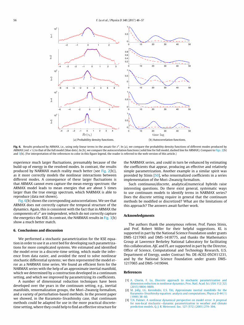
(a) Probability density functions. (b) Autocorrelation functions.

Fig. 6. Results produced by ARMAX, i.e., using only linear terms in the ansatz for zn . In (a), we compare the probability density functions of different modes produced byARMAX (red⇥’s) to that of the full model (blue dots). In (b), we compare the autocorrelation functions (solid line for full model, dashed line for ARMAX). Compare to Figs. 2(b)and 3(b). (For interpretation of the references to color in this figure legend, the reader is referred to the web version of this article.)

experience much larger fluctuations, presumably because of thebuild-up of energy in the resolved modes. In contrast, the resultsproduced by NARMAX match reality much better (see Fig. 2(b)),as it more correctly models the nonlinear interactions betweendifferent modes. A consequence of these larger fluctuations isthat ARMAX cannot even capture the mean energy spectrum: theARMAX model leads to mean energies that are about 5 timeslarger than the true energy spectrum, which NARMAX is able toreproduce (data not shown).

Fig. 6(b) shows the corresponding autocorrelations.We see thatARMAX does not correctly capture the temporal structure of thedynamics. Again, this is consistent with the fact that in ARMAX thecomponents of zn are independent, which do not correctly capturethe energetics the KSE. In contrast, the NARMAX results in Fig. 3(b)show a much better match.

6. Conclusions and discussion

We performed a stochastic parametrization for the KSE equa-tion in order to use it as a test bed for developing such parametriza-tions for more complicated systems. We estimated and identifiedthe model error in a discrete-time setting, which made the infer-ence from data easier, and avoided the need to solve nonlinearstochastic differential systems; we then represented themodel er-ror as a NARMAX time series. We found an efficient form for theNARMAX series with the help of an approximate inertial manifold,which we determined by a construction developed in a continuumsetting, and which we improved by parametrizing its coefficients.

A number of dimensional reduction techniques have beendeveloped over the years in the continuum setting, e.g., inertialmanifolds, renormalization groups, the Mori–Zwanzig formalism,and a variety of perturbation-based methods. In the present paperwe showed, in the Kuramoto–Sivashinsky case, that continuummethods could be adapted for use in the more practical discrete-time setting,where they couldhelp to find an effective structure for

the NARMAX series, and could in turn be enhanced by estimatingthe coefficients that appear, producing an effective and relativelysimple parametrization. Another example in a similar spirit wasprovided by Stinis [50], who renormalized coefficients in a seriesimplementation of the Mori–Zwanzig formalism.

Such continuous/discrete, analytical/numerical hybrids raiseinteresting questions. Do there exist general, systematic waysto use continuum models to identify terms in NARMAX series?Does the discrete setting require in general that the continuummethods be modified or discretized? What are the limitations ofthis approach? The answers await further work.

Acknowledgments

The authors thank the anonymous referee, Prof. Panos Stinis,and Prof. Robert Miller for their helpful suggestions. KL issupported in part by the National Science Foundation under grantsDMS-1217065 and DMS-1418775, and thanks the MathematicsGroup at Lawrence Berkeley National Laboratory for facilitatingthis collaboration. AJC and FL are supported in part by the Director,Office of Science, Computational and Technology Research, U.S.Department of Energy, under Contract No. DE-AC02-05CH11231,and by the National Science Foundation under grants DMS-1217065 and DMS-1419044.

References

[1] A. Chorin, F. Lu, Discrete approach to stochastic parametrization anddimension reduction in nonlinear dynamics, Proc. Natl. Acad. Sci. USA 112 (32)(2015) 9804–9809.

[2] M. Jolly, I.G. Kevrekidis, E.S. Titi, Approximate inertial manifolds for theKuramoto–Sivashinsky equation: analysis and computations, Physica D 44 (1)(1990) 38–60.

[3] T.N. Palmer, A nonlinear dynamical perspective on model error: A proposalfor non-local stochastic—dynamic parametrization in weather and climateprediction models, Q. J. R. Meterorol. Soc. 127 (572) (2001) 279–304.

F. Lu et al. / Physica D 340 (2017) 46–57 57

[4] D. Wilks, Effects of stochastic parameterizations in the Lorenz’96 system, Q. J.R. Meteorol. Soc. 131 (606) (2005) 389–407.

[5] H. Arnold, I. Moroz, T. Palmer, Stochastic parametrization and modeluncertainty in the Lorenz’96 system, Phil. Trans. R. Soc. A 371 (2013)20110479.

[6] D. Crommelin, E. Vanden-Eijnden, Subgrid-scale parameterization withconditional Markov chains, J. Atmos. Sci. 65 (8) (2008) 2661–2675.

[7] F. Kwasniok, Data-based stochastic subgrid-scale parametrization: an ap-proach using cluster-weighted modeling, Phil. Trans. R. Soc. A 370 (2012)1061–1086.

[8] A. Majda, J. Harlim, Physics constrained nonlinear regression models for timeseries, Nonlinearity 26 (1) (2013) 201–217.

[9] A. Chorin, O. Hald, Estimating the uncertainty in underresolved nonlineardynamics, Math. Mech. Solids 19 (1) (2014) 28–38.

[10] M. Chekroun, D. Kondrashov, M. Ghil, Predicting stochastic systems by noisesampling, and application to the El Niño-Southern Oscillation, Proc. Natl. Acad.Sci. USA 108 (2011) 11766–11771.

[11] J. Duan, B. Nadiga, Stochastic parameterization for large eddy simulation ofgeophysical flows, Proc. Amer. Math. Soc. 135 (4) (2007) 1187–1196.

[12] A. Du, J. Duan, A stochastic approach for parameterizing unresolved scales ina system with memory, J. Algorithm Comput. Technol. 3 (3) (2009) 393–405.

[13] J. Harlim, Model error in data assimilation, in: C. Franzke, T. O’Kane (Eds.),Nonlinear and Stochastic Climate Dynamics, Cambridge University Press,Oxford, 2016, in press.

[14] D. Kondrashov, M. Chekroun, M. Ghil, Data-driven non-Markovian closuremodels, Physica D 297 (2015) 33–55.

[15] V. Yakhot, Large-scale properties of unstable systems governed by theKuramoto–Sivashinksi equation, Phys. Rev. A 24 (1) (1981) 642.

[16] M. Schmuck, M. Pradas, S. Kalliadasis, G. Pavliotis, New stochastic modereduction strategy for dissipative systems, Phys. Rev. Lett. 110 (24) (2013)244101.

[17] M. Schmuck, M. Pradas, G. Pavliotis, S. Kalliadasis, A new mode reductionstrategy for the generalized Kuramoto–Sivashinsky equation, IMA J. Appl.Math. 80 (2) (2015) 273–301.

[18] S. Toh, Statistical model with localized structures describing the spatio-temporal chaos of Kuramoto–Sivashinsky equation, J. Phys. Soc. Japan 56 (3)(1987) 949–962.

[19] M. Rost, J. Krug, A particle model for the Kuramoto–Sivashinsky equation,Physica D 88 (1) (1995) 1–13.

[20] P. Stinis, Stochastic optimal prediction for the Kuramoto–Sivashinskyequation, Multiscale Model. Simul. 2 (4) (2004) 580–612.

[21] R. Zwanzig, Nonequilibrium Statistical Mechanics, Oxford University Press,USA, 2001.

[22] A. Chorin, O. Hald, R. Kupferman, Optimal prediction with memory, Physica D166 (3) (2002) 239–257.

[23] A. Chorin, O. Hald, Stochastic tools in Mathematics and Science, third ed.,Springer, New York, NY, 2013.

[24] P. Constantin, C. Foias, B. Nicolaenko, R. Temam, Integral Manifolds andInertial Manifolds for Dissipative Partial Differential Equations, in: AppliedMathematics Sciences, No. 70, Springer, Berlin, 1988.

[25] J. Goodman, Stability of the Kuramoto–Sivashinsky and related systems,Comm. Pure Appl. Math. 47 (3) (1994) 293–306.

[26] J. Bronski, T. Gambill, Uncertainty estimates and L2 bounds for theKuramoto–Sivashinsky equation, Nonlinearity 19 (9) (2006) 2023.http://stacks.iop.org/0951-7715/19/i=9/a=002.

[27] J. Hyman, B. Nicolaenko, The Kuramoto–Sivashinsky equation: a bridgebetween PDE’s and dynamical systems, Physica D 18 (1) (1986) 113–126.

[28] J.-P. Eckmann, D. Ruelle, Ergodic theory of chaos and strange attractors, Rev.Modern Phys. 57 (3) (1985) 617.

[29] L.-S. Young, Mathematical theory of Lyapunov exponents, J. Phys. A Math.Theor. 46 (25) (2013) 254001.

[30] S. Cox, P. Matthews, Exponential time differencing for stiff systems, J. Comput.Phys. 176 (2) (2002) 430–455.

[31] A. Kassam, L. Trefethen, Fourth-order time stepping for stiff PDEs, SIAM J. Sci.Comput. 26 (4) (2005) 1214–1233.

[32] S. Orszag, On the elimination of aliasing in finite-difference schemesby filtering high-wavenumber components, J. Atmos. Sci. 28 (6) (1971)1074–1074.

[33] D. Gottlieb, S. Orszag, Numerical Analysis of Spectral Methods: Theory andApplications, SIAM, Philadelphia, 1977.

[34] Y. Pokern, A. Stuart, P. Wiberg, Parameter estimation for partially observedhypoelliptic diffusions, J. R. Stat. Soc. B 71 (1) (2009) 49–73.

[35] A. Samson, M. Thieullen, A contrast estimator for completely or partiallyobserved hypoelliptic diffusion, Stochastic Process. Appl. 122 (7) (2012)2521–2552.

[36] P. Kloeden, E. Platen, Numerical Solution of Stochastic Differential Equations,third ed., Springer, Berlin, 1999.

[37] G. Milstein, M. Tretyakov, Stochastic Numerics for Mathematical Physics,Springer-Verlag, 2004.

[38] S. Billings, Nonlinear System Identification: NARMAX Methods in The Time,Frequency, and Spatiotemporal Domains, John Wiley and Sons, 2013.

[39] E. Hannan, The identification and parameterization of ARMAX and state spaceforms, Econometrica 44 (1976) 713–723.

[40] J. Fan, Q. Yao, Nonlinear Time Series: Nonparametric and Parametric Methods,Springer, New York, NY, 2003.

[41] J. Robinson, Inertial manifolds for the Kuramoto–Sivashinsky equation, Phys.Lett. A 184 (2) (1994) 190–193.

[42] R. Temam, X. Wang, Estimates on the lowest dimension of inertial manifoldsfor the Kuramoto–Sivashinsky equation in the general case, DifferentialIntegral Equations 7 (3–4) (1994) 1095–1108.

[43] M. Jolly, R. Rosa, R. Temam, Evaluating the dimension of an inertial manifoldfor the Kuramoto–Sivashinsky equation, Adv. Differential Equations 5 (1–3)(2000) 31–66.

[44] M. Jolly, I. Kevrekidis, E. Titi, Preserving dissipation in approximate inertialforms for the Kuramoto–Sivashinsky equation, J. Dynam. Differential Equa-tions 3 (2) (1991) 179–197.

[45] R. Rosa, Approximate inertial manifolds of exponential order, Discrete Contin.Dyn. Syst. 3 (1) (1995) 421–448.

[46] C. Foias, O. Manley, R. Temam, Modelling of the interaction of smalland large eddies in two dimensional turbulent flows, RAIRO-Modélisationmathématique et analyse numérique 22 (1) (1988) 93–118.

[47] J. Hamilton, Time Series Analysis, Princeton University Press, Princeton, NJ,1994.

[48] F. Ding, T. Chen, Identification of Hammerstein nonlinear ARMAX systems,Automatica 41 (9) (2005) 1479–1489.

[49] P. Brockwell, R. Davis, Introduction to Time Series and Forecasting, Springer,New York, NY, 2002.

[50] P. Stinis, Renormalized Mori–Zwanzig reduced models for systems withoutscale separation, Proc. R. Soc. Lond. Ser. A Math. Phys. Eng. Sci. 471 (2015)20140446.