D. R. WiltonECE Dept.

ECE 6382 ECE 6382

Green’s Functions in Two and Three Dimensions

Static Potential of Point SourcesStatic Potential of Point Sources

0

2

0

( ) ,4

V

Q

Q

r r

rr r

It is well known that the free space static potential at an observation

point due to a point charge at is

On the other hand, should also satisfy Poisson's equation,

V

V Q

where is the volume charge density. Ques : How can we

define so as to incorporate a point charge, ?

We usually avoid explicitly introducing point charges into Poisson's

equation be

caus V

Q

e the volume charge density of a point charge is

except the charge location, where it is

(i.e., a finite charge exists within a volume of zero ).

zero everywhere infinite

Representation of Point Sources Representation of Point Sources

( ) ( ) ( )V Q x x y y z z

But we mathematically represent a point charge as a volume

charge density using delta functions. Setting

we can easily check that evaluating the net charge by integrating

can

( ) ( ) )

( )

(yz x

z y x

Q x x y y z z dxdydz Q

r

over any non- vanishing volume about yields the correct total charge :

Ques : Do units on RHS and LHS agree in the above eqs.?

Thus we can

2

0

2 2 20 0

( ) ( ) ( )

( )4 4 ( ) ( ) ( )

Qx x y y z z

Q Q

x x y y z z

rr r

say that the solution to Poisson's equation,

is

22

2( , , )x y z

Superposition of PotentialsSuperposition of Potentials

0

( )

( )( ) .

4

V

V

V

dq

V

dq dV

dVd

r

rr

r r

We further say that in a volume with a

distributed volume source density , every

infinitesimal volume element of charge,

, produces a potential

By th

0

0

( )( )

4

1( ) ( )

4

V

V

V

dV

r

rr r

r rr r

e linearity of the Poisson operator, we conclude by

that

is an integration of with a weighting factor , t

superimposing

the contributions of all sources

r r

he

potential at of a unit charge at .

rr

r r

V dV

V

O

A Green’s FunctionA Green’s Function

0

1( , )

4

( ) ( , ) ( )

( , )

V

V

G

G dV

G

r rr r

r r r r

r r r

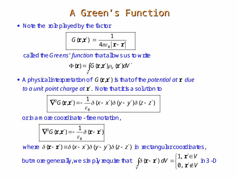
Note the role played by the factor

called the that allows us to write

A physical interpretation of is that of the

Greens' function

potential at du

2

0

2

0

.

1( , ) ( ) ( ) ( )

1( , ) ( )

( ) ( ) ( ) ( )

G x x y y z z

G

x x y y z z

r

r r

r r r r

r r

Note that it is a solution to

or in a more coordinate - free notation,

where in rect

e

to a unit point charge at

1,( )

0,V

VdV

V

rr r

r

angular coordinates,

but more generally, we simply require that in 3 -D

Green’s Function ConditionsGreen’s Function Conditions

0 0

2

1 1( , )

4 4

( , ) 0

(

Gr

G r

G

r

r 0r

r 0

To check our claims, it suffices to place at the coordinate origin so

spherical coordinates can be used :

Check that satisfies the homogeneous equation when :

2

22 2

0

1 1 1, )

4

G rr

r r r r r

r 02r

20

2

0 0

2

0 0 0

2

0

1 00, 0

4

1 1( , ) ( ) ,

ˆlim ( , ) lim ( , ) lim ( , )

( , )ˆ ˆlim sin

V V

rV V V

r

rr

G dV dV V

G dV G dV G dS

Gd d

r

r 0 r r 0

r 0 r 0 r 0 n

r 0r r

divergencetheorem

Next, check that encloses :

2

00 0

4lim

4 2

0 2

0

1,

.V

r 0 if encloses

r̂V

V

Green’s Function for a General Linear OperatorGreen’s Function for a General Linear Operator

( , ) ( )G

r r r r

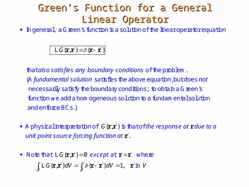
In general, a Green's function is a solution of the linear operator equation

that of the problem.

(A satisfies the above e

L

also satisfies any boundary conditions

fundamental solution

quation, but does

necessarily satisfy the boundary conditions; to obtain a Green's

function we add a homogeneous solution to a fundamental solution

and enforce BCs.)

A physical interpreta

not

( , )

.

( , ) 0

( , ) ( ) 1,V V

G

G

G dV dV V

r r r

r

r r r r

r r r r r

tion of is that of

Note that at where

in

L

L

the response at due to a

unit point source forcing function at

except

A Source-Weighted Superposition over the Unit A Source-Weighted Superposition over the Unit Source Response Provides a General Solution Source Response Provides a General Solution

( ) ( ) , ( )

( ) ( , ) ( )V

u f f

u G f dV

r r r

r r r r

The solution to the general problem

a general forcing function,

is then found by a source - weighted superposition of the f 'n response :

To check that this is

-

a so

Lu

u

( ) ( , ) ( ) ( , ) ( )

( ) ( )

( )

V V

V

u G f dV G f dV

f dV

f

r r r r r r r

r r r

r

lution, note that

Lu L L

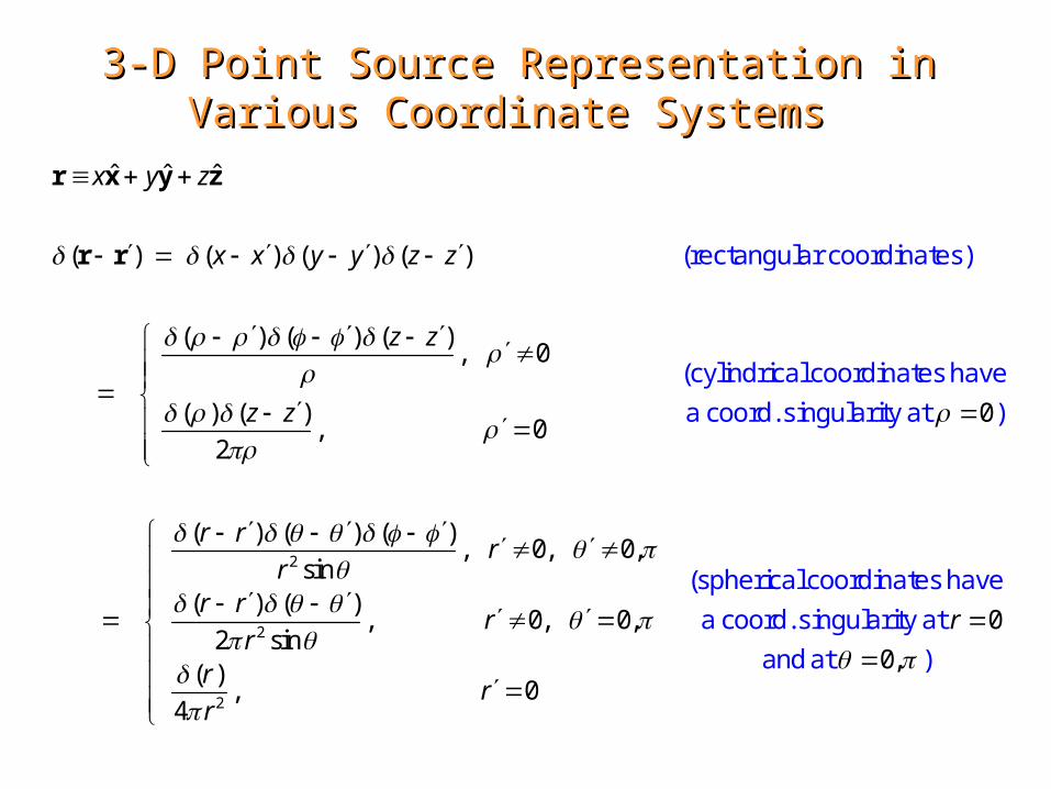
3-D Point Source Representation in Various 3-D Point Source Representation in Various Coordinate Systems Coordinate Systems

ˆ ˆ ˆ

( ) ( ) ( ) ( )

( ) ( ) ( ), 0

( ) ( ) 0, 0

2

( ) ( ) (

x y z

x x y y z z

z z

z z

r r

r x y z

r r (rectangular coordinates)

(cylindrical coordinates have

a coord. singularity at )

2

2

2

), 0, 0,

sin( ) ( )

, 0, 0, 02 sin

0,( ), 0

4

rr

r rr r

rr

rr

(spherical coordinates have

a coord. singularity at

and at )

2-D Line Source Representation in Various 2-D Line Source Representation in Various Coordinate Systems Coordinate Systems

ˆ ˆ

( ) ( ) ( )

( ) ( ), 0

( ) 0, 0

2

x y

x x y y

r x y

r r (rectangular coordinates)

(cylindrical coordinates have

a coord. singularity at )

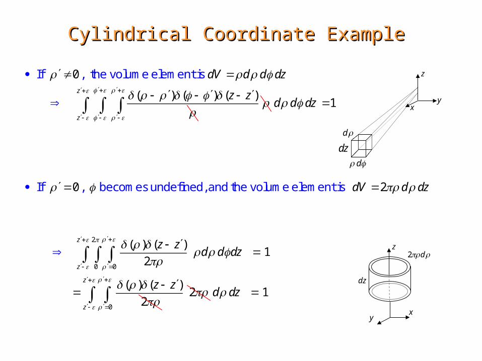
Cylindrical Coordinate ExampleCylindrical Coordinate Example

0

( ) ( ) ( )

dV d d dz

z z

If , the volume element is

2

0 0

1

0 2

( ) ( )1

2

( ) ( )

2

z

z

z

z

d d dz

dV d dz

z zd d dz

z z

If , becomes undefined, and the volume element is

20

1z

z

d dz

d

d dz

xy

z

dz

2 d z

xy

Example: A Simple Static Green’s Function with Example: A Simple Static Green’s Function with Boundary Conditions --- Charge over a Ground Boundary Conditions --- Charge over a Ground

PlanePlane

0 0

( , )

1 1( , )

4 4fundamental solution homogeneous soluti

The potential at due to a unit charge at

can be found from image theory. It is given by

G

G

r r r r

r rr r r r

above a ground plane

2 2

0 0 0

ˆ2 .

0 ( , )

1 1 1( , ) ( , ) ( , ) 0, 0

4

( , ) 0 0

onwhere

Note that for in the upper half space ( ), satisfies

(since )

at (since

z

z G

G z

G z

r r z

r r r

r r r r r rr r

r r r r r

and

0at ).z r

1 [C]r r

z

0 on ground plane

1 [C]r r

z

0 on ground plane

r

r r

-1 [C]

r r

Static Green’s Function with Boundary Static Green’s Function with Boundary Conditions (cont.)Conditions (cont.)

0

( )

1 1 1( ) ( , ) ( ) , ( , )

4

ˆ2 0

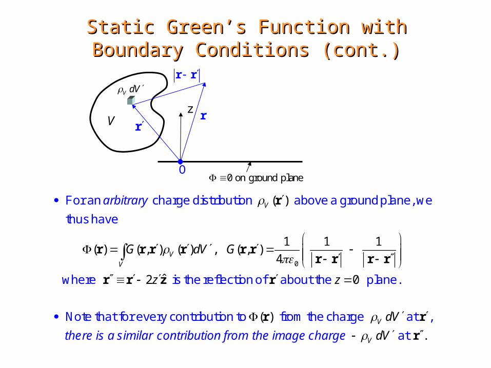
For an charge distribution above a ground plane, we

thus have

where is the reflection of about the plane.

V

V

V

G dV G

z z

r

r r r r r rr r r r

r r z r

arbitrary

( )

.

Note that for every contribution to from the charge at ,

at V

V

dV

dV

r r

r there is a similar contribution from the image charge

z

0 on ground plane

rr

r r

V dV

V

O

Example: Scalar Point Source in a Rectangular WaveguideExample: Scalar Point Source in a Rectangular Waveguide

2 2

2 2

( ) ( ) ,

( ) 0, 0, ; 0, ;

( , ) ( , )

i te

k f kv

x a y b z

G k G

r r r

r

r r r r r

We assume an time dependence and

a scalar wavefunction that satisfies

Hence the Green's function for the problem satisfies

2

22

,

( , ) 0, 0, ; 0, ;

( , )

0 sin ,x x

x x y y z z

G x a y b z z z

G X x Y y Z z

d Xk X X x A k x k

dx

r

r r

r r

with waves outgoing from

Assuming a separation - of - variables form

and applying boundary conditions yie

lds

22

2

2 2 2 2 2 22

22

2 2 2 2 2 2

, 1,2,

0 sin , , 1,2,

,,0 ,

, ,

z

z

x

y y y

ik z zx y x y

z zik z z

x y x y

mm

a

d Y nk Y Y y B k y k n

dy b

k k k k k kCe z zd Zk Z Z z k

dz De z z i k k k k k k

x , y ,z

y

z

x

a

b

Point Source in a Waveguide, cont’dPoint Source in a Waveguide, cont’d

,

,

1 1

1 1

2 2 2 22 2

,2 2 2 22 2

( , )

sin sin ,

( , )

sin sin ,

,

,

z mn

z mn

ik z z

mnm n

ik z z

mnm n

z mn

G

m x n yA e z z

a bG

m x n yB e z z

a b

k m a n b k m a n bk

i m a n b k k m a n b

r r

r r

Hence is of the form

0

1 1 1

( , ) lim

( , , ; , , ) ( , , ; , , ) ,

sin sin sin sinmn mnn m n

G z z z z

G x y z x y z G x y z x y z x y

m x n y m x n yA B

a b a b

r rContinuity of at requires ( )

(also derivatives w.r.t. are continuous!)

,

1

1 1

( , ) sin sin z mn

mn mnm

ik z zmn

m n

A B

m x n yG A e

a b

r r

x , y ,z

y

z

x

a

b

,

,

,

,

,

z mn

z mn

z mn

ik z zik z z

ik z z

e z ze

e z z

Point Source in a Waveguide, cont’dPoint Source in a Waveguide, cont’d

,

1 1

2 2

( , ) sin sin

( , ) ( , )

To determine the constants , note first that

To evaluate the LHS, note that

z mnik z zmn

m n

mn

z z

z z

m x n yG A e

a b

A

G k G dz x x y y z z dz

x x y y

r r

r r r r

2 2 22

2 2 2

2

2 0

, ,1 1 1 1

,1 1

,

( , ) ( , , ; ) ( , , ; )lim

sin sin sin sin

2 sin sin

z

z

z mn mn z mn mnm n m n

z mn mnm n

x y z

G G x y z G x y zdz

z z z

m x n y m x n yik A ik A

a b a b

m x n yik A

a b

r r r r

-

2 22

2 2

( , ) ( , )( , ) 0

( , ) ,

Note

since and hence w.r.t. are continuous at

z z z

z z z

G Gdz dz k G dz

x y

G x y z z

r r r r

r r

r r

-

its derivatives

Key result!

Key observation!

Point Source in a Waveguide, cont’dPoint Source in a Waveguide, cont’d

,

1 1

,1 1

2 2 ( , , ; ) ( , , ; )( , ) ( , )

( , ) sin sin

2 sin sin

z mnik z zmn

m n

z mn mnm n

z

z

G x y z G x y zG k G dzz z x x y y

m x n yG A e

a b

m x n yik A x x y y

a b

r rr r r r

r r

Hence

0 0

sin

sin sin sin sin4

"

mn

b a

mp nq

z

z

z z dz

A

p x m x q y n y abdxdy

a a b b

Finally, to determine use the orthogonality properties of the functions :

Project" both sides of the above onto the

,,

,

sin sin ,

, ,

22 sin sin sin sin

4

2( , ) sin sin sin

z mn mn mnz mn

z mn

p x q y

a bp m q n

ab m x n y m x n yik A A

a b ik ab a b

m x m x nG

ik ab a a

r r

functions use the

orthogonality properties, and finally substitute to obtain

,

1 1

sin z mnik z z

m n

y n ye

b b

2D Sources 2D Sources

( ) ( ) ( )

( ) ( ), 0

( ), 0

2

( ) ( )S

x x y y

dS dxdy

r r

r r r r

or

o

A two - dimensional (no - variation) "point" source

is actually a with unit line source density :

z

line source

( )

1,

0,

d d

S

S

S xy

r r

r

r

r

It is often convenient to treat the integration over in the -plane as a

integration over, say, a circular cylinder of and radius

volume unit height

.r centered about the point

ˆ ˆx y r x y(Reminder : In 2D, )

1[m]x

z

y

r

Example: Green’s Function for 2D Poisson’s Example: Green’s Function for 2D Poisson’s EquationEquation

2 2 22 2

2 2 2 20

0

1 1,

1( , ) ln

2

:

v

x y

G

r r

2 - D Poisson's equation

is the Green's

function for the 2D Poisson's equation with

unit line source density alon

Claim:

static

2

0 0

( ) ( )( , )

2

ˆˆ ˆ

G

x y

z

rr r

r x y ρ

g the - axis,

(Reminders : In 2 - D, ; here we have

neither a nor a variation!)

z

1[m]

y

x

z

““Proof” of Claim Proof” of Claim

0

( , )

1 1 1

2

G

d dG d

d d d

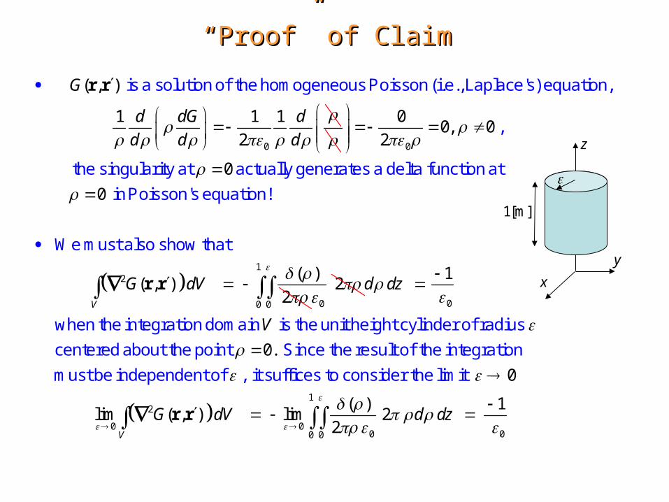
r r is a solution of the homogeneous Poisson (i.e., Laplace's) equation,

0

2

00, 0

2

0

0

( )( , )

2V

G dV

r r

,

the singularity at actually generates a delta function at

in Poisson's equation!

We must also show that

0

2

1

00 0

1

0.

d dz

V

when the integration domain is the unit height cylinder of radius

centered about the point Since the result of the integration

must be independent of , it suffices to c

1

2

0 00 00 0

0

( ) 1lim ( , ) lim 2

2V

G dV d dz

r r

onsider the limi

t

1[m]

y

x

z

““Proof” of Claim (cont.)Proof” of Claim (cont.)

2

0

0 0

2

0 0

lim ( , )

1 1ˆ( , ) ln , ( , )

2 2

lim ( , ) lim ( , )

V

V

G dV V

G G

G dV G

r r

r r r r ρ

r r r r

" f

To evaluate , unit height cylinder of radius , we note that

Hence th

e integral above is

0

00

ˆlim ( , )

1 1lim

2

V

V V dS

dV

G d dz

r r n

lux per unit vol. "

Flux

div thm.

boundary of

ˆ ˆ ρ ρ

1 2

00 0

12

0 00 00 0

1

( ) 1lim ( , ) lim 2

2V

d dz

G dV d dz

r r

Therefore we have finally,

ˆV V

dV dS

A A n

" Flux per Flux unit vol. "

div thm.

Solution Is Easily Extended to 2D Sources Off Solution Is Easily Extended to 2D Sources Off the the zz-Axis -Axis

0

2

0

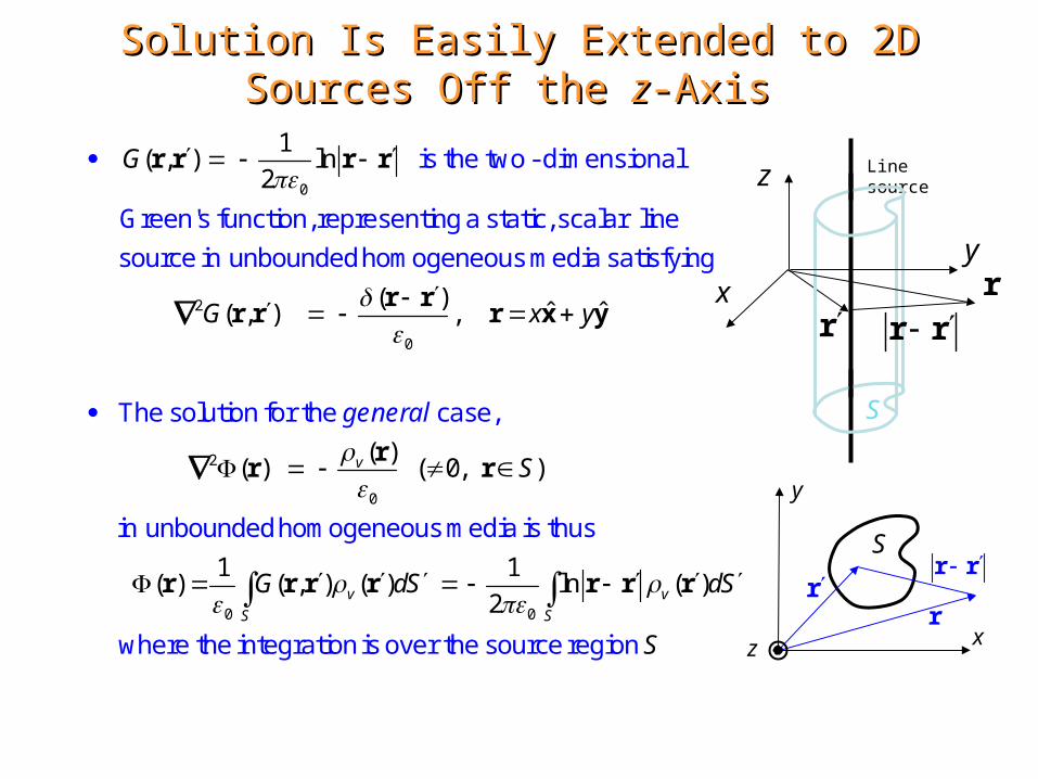
1( , ) ln

2

( )ˆ ˆ( , ) ,

G

G x y

r r r r

r rr r r x y

is the two - dimensional

Green's function, representing a static, scalar line

source in unbounded homogeneous medi

a satisfying

The solution

for

2

0

0 0

( )( ) ( 0, )

1 1( ) ( , ) ( ) ln ( )

2

v

v v

S S

S

G dS dS

S

rr r

r r r r r r r

the case,

in unbounded homogeneous media is thus

where the integration is over the source region

general

x

r r

y

rr

S

z

x

z

y

rr

Line source

r r

S

Example: Green’s Function for 2D Wave EquationExample: Green’s Function for 2D Wave Equation

(2)0

2 2

( )( , )

4

( )( , ) ( , ) ( )

2

H kG

i

G k G

r r

r r r r r

is the

Green's function for the 2D wave equation

with unit line source density along the - axis,

and a harmonic tim

outgoing - wave

z

Claim:

(2)0

2

.

ˆˆ ˆ

( )

10

i te

x y

z

H k

d dyk y

d d

r x y ρ

e variation of the form

(Reminders : In 2D, ; here we have

neither a nor a variation!)

The solution of Bessel's equation,

, which is singular at 0, actually

generates a delta function there!

1[m]

y

x

z

““Proof” of Claim Proof” of Claim

2 2

(2)0

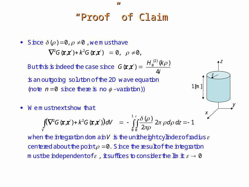
( ) 0, 0 ,

( , ) ( , ) 0, 0,

( )( , )

4

0

G k G

H kG

i

n

r r r r

r r

Since we must have

But this is indeed the case since

is an outgoing solution of the 2D wave equation

(note since there is no - variatio

1

2 2

0 0

( )( , ) ( , ) 2 1

2

0.

V

G k G dV d dz

V

r r r r

n))

We must next show that

when the integration domain is the unit height cylinder of radius

centered about the point Since the result of t

0 he integration

must be independent of , it suffices to consider the limit

1[m]

y

x

z

““Proof” of Claim (cont.)Proof” of Claim (cont.)

2 2

0lim ( , ) ( , )

0V

G k G dV V

r r r r

Evaluate , unit height cylinder of radius

Since we are integrating over a region near the origin , we may use

small argument approximations to the Hankel functi

0 0

2

0 0

21 ln

( ) ( ) 12ˆ( , ) , ( , )

4 4 2

lim ( , ) lim ( , ) limV V

ki

J k iN kG G

i i

G dV G dV

r r r r ρ

r r r r

" Flux per unit vol. "

div thm.

on,

Hence the first integral above is

0

1 2

00 0

1 202 2

0 00 0 0

2 2

00

ˆ( , )

1ˆ ˆlim 1

2

lnlim ( , ) lim

2

lim ln 0 ( , )

V V

V

G dS

d dz

k G dV k d d dz

k G

r r n

ρ ρ

r r

r r

Flux

boundary of

whereas the second i

s

2 ( , ) 1,V

k G dV V r r r

ˆV V

dV dS

A A n

" Flux per Flux unit vol. "

div thm.

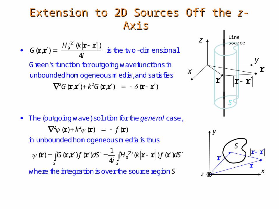
Extension to 2D Sources Off the Extension to 2D Sources Off the zz-Axis -Axis

(2)0

2 2

( )( , )

4

( , ) ( , ) ( )

is the two - dimensional

Green's function for outgoing wavefunctions in

unbounded homogeneous media, and satisfies

The (outgoing wave) solution

f

H kG

i

G k G

r rr r

r r r r r r

2 2

(2)0

( ) ( ) ( )

1( ) ( , ) ( ) ( ) ( )

4

or the case,

in unbounded homogeneous media is thus

where the integration is over the source region S S

k f

G f dS H k f dSi

S

r r r

r r r r r r r

general

x

r r

y

rr

S

z

x

z

y

rr

Line source

r r

S

Summary of Common 2D, 3D Greens FunctionsSummary of Common 2D, 3D Greens Functions

2 2

(2)0

2

2 2

2

0

( , ) ( , ) ( )

( )( , )

4

( , ) ( )

1( , ) ln

2

( , ) ( , ) ( )

( , )4

( ,

( )

) ( )

1( , )

4

ik

z z

G k G

H kG

i

G

G

G k G

eG

G

G

r r

r r r r r r

r rr r

r r r r

r r r r

r r r r r r

r rr r

r r r r

r rr r

2-D :

3 -D :

x

z

y

rr

Line source

r r

x

r r

y

r

r

z

Point source

These Green’s functions are actually fundamental solutions since there areno imposed boundary conditions

Line Source Illumination of a Circular Cylinder Line Source Illumination of a Circular Cylinder

x

y

a

Line source

(2)0inc ( )

ˆ( ) ,4

z

H k

i

r r

r r x

A line source illuminates a circular cylinder;

both are parallel to the -axis. Hence the

incident field is

The field satisfies the Dirichlet boundary

condition

totalinc sca

2 sca 2 sca

( ) ( ) ( ) 0

( ) ( ) 0.

a

k

r r r

r r

at

on the cylinder surface.

The scattered field is source - free and hence is an

outgoing solution to

In cylindrical coordinates it must have th r

e fo

sca (2)

0

( ) ( ) inn n

n

a H k e

r

m

The Addition TheoremThe Addition Theoreminc

(2) ( )

(2)0

( )

0.

( ) ( ) ,

( )

(

inn n

n

n

x y

H k J k e

H k

J k

r

r r

We need an expansion for in terms of cylindrical wavefunctions

about Such an expansion is provided by the addition theorem

(2) ( )) ( ) ,

0.

inn

n

H k e

x

where is the angular position of the line source relative to the -axis. For

our problem,

The addition theorem is analogous to the Laurent expansion abo

1

0

1

0

,1

,

n n

n

n n

n

z z

z z z z

z zz z z z

ut the origin

of a simple pole at :

x

y

Solution of the Line Source Scattering Problem Solution of the Line Source Scattering Problem

inc sca (2) (2)

(2)

(2)

:

1( ) ( ) ( ) ( ) ( ) 0

4

( ) ( )

4 (

in inn n n na

n n

n nn

n

a

J ka H k e a H ka ei

J ka H ka

i H k

r r

The addition theorem allows us to easily apply the Dirichlet boundary

condition at

(2)(2) (2)

(2)

(2)(2)

(2)

)

( ) ( )1( ) ( ) ( ) ,

4 ( )( , )

( ) ( )1( ) ( ) ,

4 ( )

inn nn n n

n n

inn nn n

n n

a

J ka H kH k J k H k e

i H ka

J ka H kJ k H k e

i H ka

The total field is thus

Interpretation as a Green’s FunctionInterpretation as a Green’s Function

The source is a unit strength line source

We can obtain the result for a line source

the x -axis by simply replacing by

Hence a Green's function for the cylinder scattering problem is

off

(2)(2) (2)

(2)

(2)(2)

(2)

(2)0

( ) ( )1( ) ( ) ( ) ,

4 ( )( , )

( ) ( )1( ) ( ) ,

4 ( )

( )

4fundamentalsolution

inn nn n n

n n

inn nn n

n n

J ka H kH k J k H k e

i H kaG

J ka H kJ k H k e

i H ka

H k

i

r r

r r

(2)

(2)(2)

( ) ( )1( )

4 ( )homogeneous solution

inn nn

n n

J ka H kH k e

i H ka

Line source

x

y

a