cusum techniques for technical trading in financial market · cusum techniques for technical...

1

CUSUM TECHNIQUES FOR TECHNICAL TRADINGIN FINANCIAL MARKET

It is discovered that the CUSUM techniques used by people in the

manufacturing industry can be adapted to yield a trading strategy in the

financial market. The filter trading strategy familiar to people in finance is

found to be a particular case of CUSUM procedures. A more general form of

the CUSUM techniques will yield new trading strategies which have intuitive

appeals . Trading characteristics of such strategies will be investigated using

CUSUM techniques.

keywords : CUSUM techniques, filter trading strategy, average run length.

1 IntroductionControl chart techniques were first developed in the 1930's. Since then it has become

an dispensable tool in the manufacturing industry used heavily in monitoring the quality of the

manufactured products. Some commonly used control charts are the Shewhart charts by

Shewhart (1939), the cumulative-sum control charts by Page (1954 a & b), the moving

average control charts and the geometric moving average control charts by Roberts (1959)

etc.

On the other hand, technical charts were very popular among people in the financial

market. A sizable proportion of traders in financial market are chartists who base their trading

strategy on price charts of the financial product. Despite the fact that the financial analysts and

quality controllers both rely on charts, they are treated as two different groups of people using

completely different techniques for their works. However, it will not take long to see that

there is a great similarity between the two charting approaches. People in quality control are

2

concerned with the quality of a product and wish to sound an early alarm when the quality is

out of control. When the quality is above (below) a target value, the control chart will

generate an upward (downward) shift warning. Upon the generation of a warning signal, the

production process has to be stopped and readjusted. For traders in the financial market, what

is important is the detection of an upward or downward price trend. Technical charts are used

to detect such trends. Whenever an upward (downward) trend is detected, the trader will take

long (short) position in the market.

Despite these similarities, linkages between the two have not been discussed in both

the quality control and financial literature. This paper will offer a first attempt to link up the

two fields of investigation. In particular, we will focus our attention to one popular trading

rule in the finance literature, which is the filter trading rule proposed by Alexander (1961). We

will show that the filter rule is equivalent to the CUSUM techniques in quality control. In

more general terms, any principle adopted in detecting a shift in product quality can also be

applied to detect upward or downward shift in prices in the financial market.

In section 2 of this paper, we will briefly review the CUSUM techniques and filter

trading rule. Then, we will show that the two approaches are equivalent. Along the line that a

quality control technique can be adopted to a trading rule in the financial market, we consider,

in section 3, the trading rule corresponding to the general CUSUM procedure and its trading

performance. Empirical evidence presented in section 4 shows that the general CUSUM

techniques also work well in the financial market and offers an improvement over the classical

filter trading rule.

The performance characteristic of a quality control technique can be described by the

average run length of the production process. The average run length has been tabulated by

Chiu (1974) for various parameter values. In section 5 of this paper, we compute the means

and variances of the run length to supplement some existing tables on the control charts

3

literature. When control chart techniques are applied to form a trading rule, the average run

length becomes important as it will be tied up with the trading profit. Given that the market is

in an upward trend, the longer is the average run length before the generation of a sell signal,

the larger is the profit. The variance of the run length will then control the variability of the

derived profit. In section 6 of this paper, the formulae derived in section 5 are used to obtain

the mean and variance of the profit of a trading strategy. The actual profit obtained empirically

can then be used to test whether the obtained profit is statistically significant or not. This could

have implications on market efficiency which is a central topic of research in the field of

finance. The paper ends with section 7 which contains a summary and discussion.

2. CUSUM techniques and filter trading rule

2.1 CUSUM techniques

CUSUM techniques were developed in the fifties, see for example Page (1954 a&b),

Kemp (1961, 1967 a&b) and the book by Van Dobben De Bruyn (1968), etc. The CUSUM

procedure is designed to detect a shift in the mean value of a measured quantity from a target

value. Consider independent observations y1, y2, ..., yn, ... arising from a manufacturing

process with mean level µ. Assume that we are interested in detecting an upward shift in the

mean level of the production process. A CUSUM procedure with parameters (k,h) that can

signal a warning of an upward shift can be described as follows. Fix a parameters k called the

reference value and a parameter h called the threshold value. Take observations y1, y2, ... and

let xi i y k= − . Quite often, k is set to be µ but, in general, k can be set at any level. The

cumulative sum is Sn = x1 + x2 + x3 + ...+ xn. Define Sn

' recursively as follows.

S

S S xn n n

0

1

0

0

'

' 'max( , )

== +

−

(1)

4

Note that Sn' = 0 whenever Sn i n i S≤

≤ ≤min0

. The CUSUM procedure would recommend

an action at the first n satisfying Sn' h≥ . The CUSUM techniques which can signal warning

of downward shift in mean value can be defined in a similar fashion.

2.2 The filter trading rule

The filter trading rule was one of the most investigated trading rule in the finance

literature. In the sixties, Alexander (1961, 1964), Fama and Blume (1966) and Dryden (1969)

considered a trading rule called the filter rule and empirically showed that after taking

transaction costs into account, the filter trading rule cannot outperform the buy-and-hold

strategy which simply buys the stock and hold it throughout the time period under

consideration. These findings lend considerable support to the market efficiency theory which

forms the basis of a wide range of research in the field of finance.

The filter trading rule is a mechanical trading rule which generates a sequence of buy

signals and sell signals alternately according to the following rule. If the daily closing price of a

particular stock moves up at least x percent from a low, a buy signal is generated. We then buy

and hold the stock until the closing price moves down at least x percent from a subsequent

high, at which time a sell signal is generated and we simultaneously sell and go short. Repeat

the process so that at the next buy signal we will cover up the short position and go long, etc.

Note that price movement of less than x percent (from a low or high) does not generate a

signal. x is called the filter size for the trading rule.

2.3 Filter rule treated as a CUSUM procedure

In this subsection, we will show that the filter rule is simply equivalent to the CUSUM

procedure. Let pt denote the closing price of a stock at day t ( t = 0, 1, 2, ...). Suppose a sell

signal has just been generated at time 0 and the filter trading rule is to generate the next buy

5

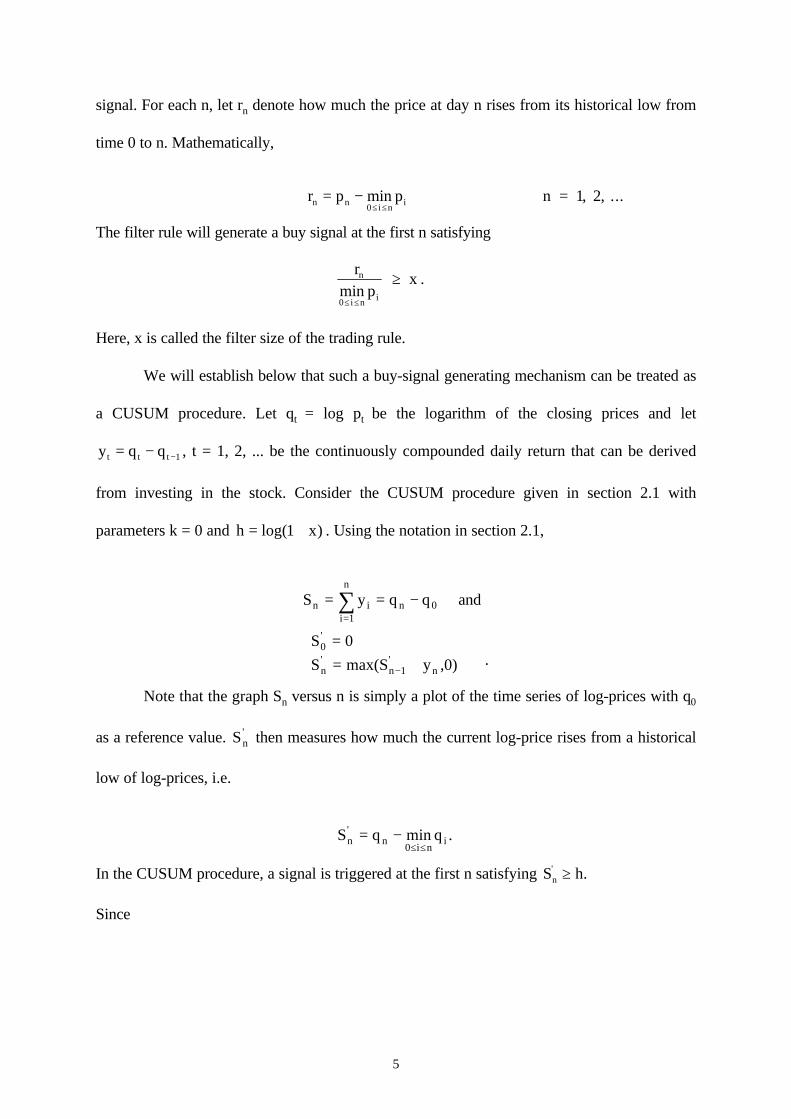
signal. For each n, let rn denote how much the price at day n rises from its historical low from

time 0 to n. Mathematically,

r p pn ni n

i= −≤ ≤

min0

1 2 n = , , ...

The filter rule will generate a buy signal at the first n satisfying

rp

n

i n imin0≤ ≤

≥ x .

Here, x is called the filter size of the trading rule.

We will establish below that such a buy-signal generating mechanism can be treated as

a CUSUM procedure. Let qt = log pt be the logarithm of the closing prices and let

y q qt t t= − −1 , t = 1, 2, ... be the continuously compounded daily return that can be derived

from investing in the stock. Consider the CUSUM procedure given in section 2.1 with

parameters k = 0 and h x= +log( )1 . Using the notation in section 2.1,

S y q q and

S 0

S max(S y ,0)

n ii 1

n

n 0

0'

n'

n 1'

n

= = −

== +

=

−

∑

.

Note that the graph Sn versus n is simply a plot of the time series of log-prices with q0

as a reference value. Sn' then measures how much the current log-price rises from a historical

low of log-prices, i.e.

S q min q .n'

n0 i n

i= −≤ ≤

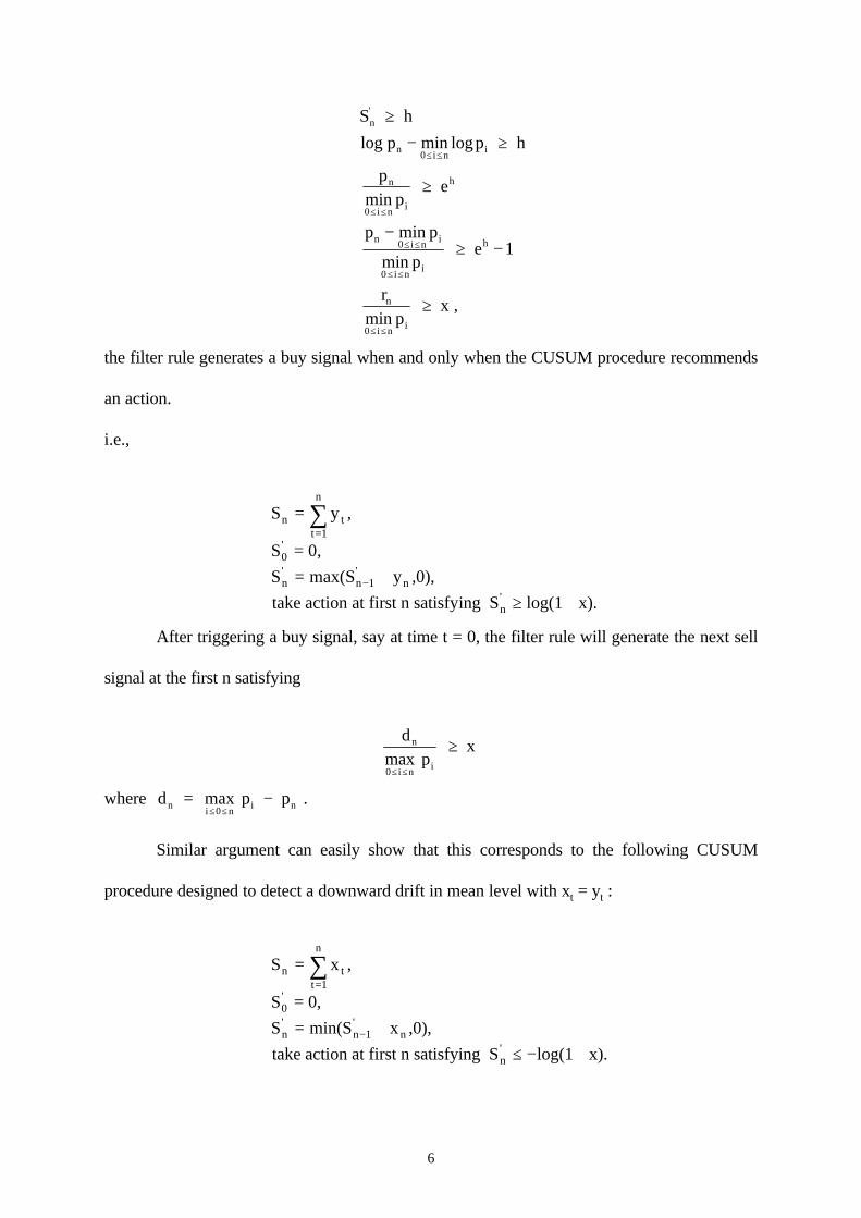
In the CUSUM procedure, a signal is triggered at the first n satisfying S h.n' ≥

Since

6

S h

log p h

e

e

x

n

n

i ni

n

i n i

h

n i n i

i ni

h

n

i n i

p

pp

p p

p

rp

'

min log

min

min

min

min,

≥

⇔ − ≥

⇔ ≥

⇔−

≥ −

⇔ ≥

≤ ≤

≤ ≤

≤ ≤

≤ ≤

≤ ≤

0

0

0

0

0

1

the filter rule generates a buy signal when and only when the CUSUM procedure recommends

an action.

i.e.,

S y ,

S 0,

S max(S y ,0),

take action at first n satisfying S log(1 x).

n tt 1

n

0'

n'

n 1'

n

n'

=

== +

≥ +

=

−

∑

After triggering a buy signal, say at time t = 0, the filter rule will generate the next sell

signal at the first n satisfying

dn

i nimax

0≤ ≤

≥ p

x

where dni n

i n p p= −≤ ≤

max0

.

Similar argument can easily show that this corresponds to the following CUSUM

procedure designed to detect a downward drift in mean level with xt = yt :

S x ,

S 0,

S min(S x ,0),

take action at first n satisfying S log(1 x).

n tt 1

n

0'

n'

n 1'

n

n'

=

== +

≤ − +

=

−

∑

7

3. Generalizing the filter trading rule

3.1 A generalized filter trading rule

The CUSUM procedure defined in section 2.1 is characterized by two parameters

(k,h), where k is the reference value and h is the threshold value. In section 2, we see that

there is a one to one correspondence between a CUSUM procedure with parameters (0,h) and

a filter trading rule with filter size x eh= − 1. Note that x ≈ h when h and x are close to zero.

Obviously, there is no reason why we should restrict ourselves to CUSUM procedure with k =

0. We can consider a general CUSUM procedure with k ≠ 0 and h > 0. Such CUSUM

procedures then give rise to a class of trading rules which is more general than the classical

filter trading rule. As far as the authors are aware, such trading rules have not appeared in

literature in financial research. The question remains as to whether such generalized filter

trading rules make enough investment sense or not.

3.2 Rational behind the trading rule

The ordinary filter rule is based on a trend following strategy. As Alexander (1961) put

it, " if the stock has moved up x% ( or move down y% ), it is likely to move up more than x%

further ( or move down more than y% further ) before it moves down by x% ( or moves up by

y% ) ". This forms the basis for using the filter rule as a practical trading rule in timing the

trading of a stock. To interpret the parameter k involved in a general filter rule, consider first

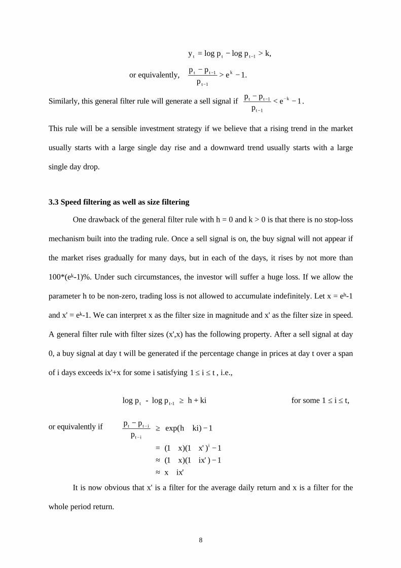
the case h = 0 and k > 0. It is easy to see that such a general filter rule will issue a buy signal

whenever the one day return exceeds k. In other words, we will buy a stock at the end of day t

whenever

8

y log p log p k,

or equivalently, p p

pe 1.

t t t 1

t t 1

t 1

k

= − >

−> −

−

−

−

Similarly, this general filter rule will generate a sell signal if p p

pet t

t

k−< −−

−

−1

1

1.

This rule will be a sensible investment strategy if we believe that a rising trend in the market

usually starts with a large single day rise and a downward trend usually starts with a large

single day drop.

3.3 Speed filtering as well as size filtering

One drawback of the general filter rule with h = 0 and k > 0 is that there is no stop-loss

mechanism built into the trading rule. Once a sell signal is on, the buy signal will not appear if

the market rises gradually for many days, but in each of the days, it rises by not more than

100*(ek-1)%. Under such circumstances, the investor will suffer a huge loss. If we allow the

parameter h to be non-zero, trading loss is not allowed to accumulate indefinitely. Let x = eh-1

and x' = ek-1. We can interpret x as the filter size in magnitude and x' as the filter size in speed.

A general filter rule with filter sizes (x',x) has the following property. After a sell signal at day

0, a buy signal at day t will be generated if the percentage change in prices at day t over a span

of i days exceeds ix'+x for some i satisfying 1 ≤ ≤i t , i.e.,

log p - log p h + kit t-1 ≥

for some 1 ≤ i ≤ t,

or equivalently if

p p

ph ki

x x

x ix

ix

t t i

t i

i

−≥ + −

+ + −≈ + + −≈ +

−

−

=

x

exp( )

( )( ' )

( )( ' )

'

1

1 1 1

1 1 1

It is now obvious that x' is a filter for the average daily return and x is a filter for the

whole period return.

9

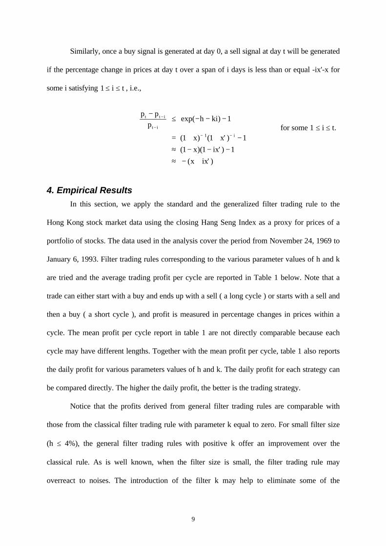
Similarly, once a buy signal is generated at day 0, a sell signal at day t will be generated

if the percentage change in prices at day t over a span of i days is less than or equal -ix'-x for

some i satisfying 1 ≤ ≤i t , i.e.,

p p

ph ki

x x

x ix

x ix

t t i

t i

−≤ − − −

= + + −≈ − − −≈ − +

−

−

− −

i

exp( )

( ) ( ' )

( )( ' )

( ' )

1

1 1 1

1 1 1

1

for some 1 ≤ i ≤ t.

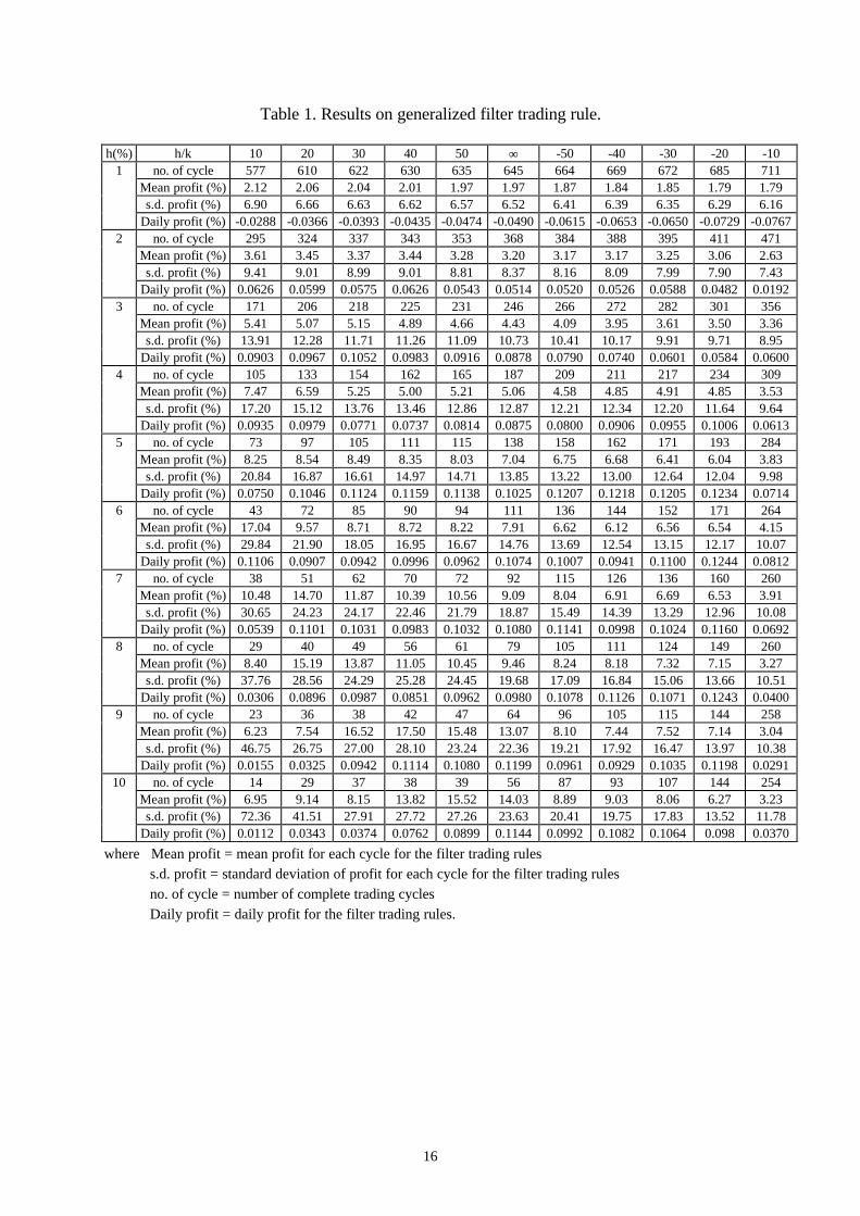
4. Empirical ResultsIn this section, we apply the standard and the generalized filter trading rule to the

Hong Kong stock market data using the closing Hang Seng Index as a proxy for prices of a

portfolio of stocks. The data used in the analysis cover the period from November 24, 1969 to

January 6, 1993. Filter trading rules corresponding to the various parameter values of h and k

are tried and the average trading profit per cycle are reported in Table 1 below. Note that a

trade can either start with a buy and ends up with a sell ( a long cycle ) or starts with a sell and

then a buy ( a short cycle ), and profit is measured in percentage changes in prices within a

cycle. The mean profit per cycle report in table 1 are not directly comparable because each

cycle may have different lengths. Together with the mean profit per cycle, table 1 also reports

the daily profit for various parameters values of h and k. The daily profit for each strategy can

be compared directly. The higher the daily profit, the better is the trading strategy.

Notice that the profits derived from general filter trading rules are comparable with

those from the classical filter trading rule with parameter k equal to zero. For small filter size

(h ≤ 4%), the general filter trading rules with positive k offer an improvement over the

classical rule. As is well known, when the filter size is small, the filter trading rule may

overreact to noises. The introduction of the filter k may help to eliminate some of the

10

unsuccessful buy-sell signals. On the other hand, when the filter size increases, the sensitivity

for detecting a small upward or downward trend will decrease. In this situation, the trading

system may not be sensitive enough for gradual increases or decreases. The introduction of a

negative filter k into the process can also help overcome this shortcoming. Therefore, for large

filter (5% ≤ h ≤ 8%), the general filter trading rules with negative parameter k perform better

than the classical filter trading rule. For very large filter size (h ≥ 8%), the general filter trading

strategy cannot outperform the classical one.

5. Run length

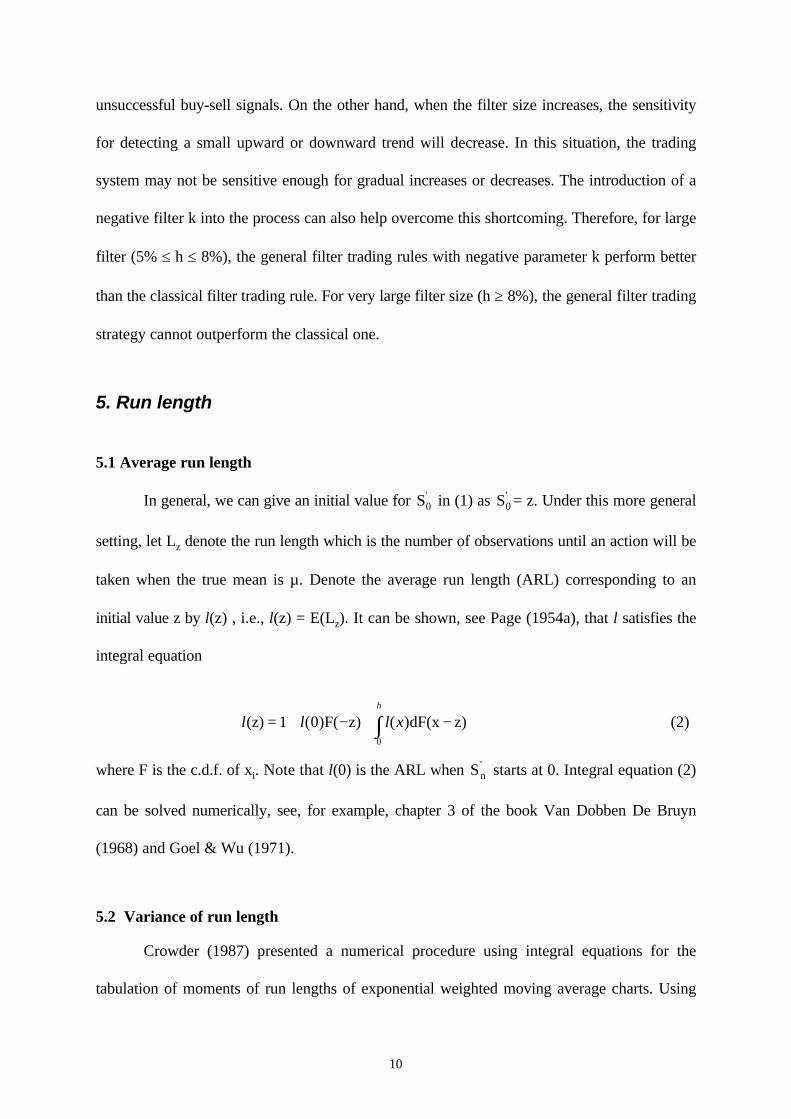
5.1 Average run length

In general, we can give an initial value for S0' in (1) as S0

' = z. Under this more general

setting, let Lz denote the run length which is the number of observations until an action will be

taken when the true mean is µ. Denote the average run length (ARL) corresponding to an

initial value z by l(z) , i.e., l(z) = E(Lz). It can be shown, see Page (1954a), that l satisfies the

integral equation

l l l xh

(z) 1 F( z) dF(x z)= + − + −∫( ) ( )00

(2)

where F is the c.d.f. of xi. Note that l(0) is the ARL when Sn' starts at 0. Integral equation (2)

can be solved numerically, see, for example, chapter 3 of the book Van Dobben De Bruyn

(1968) and Goel & Wu (1971).

5.2 Variance of run length

Crowder (1987) presented a numerical procedure using integral equations for the

tabulation of moments of run lengths of exponential weighted moving average charts. Using

11

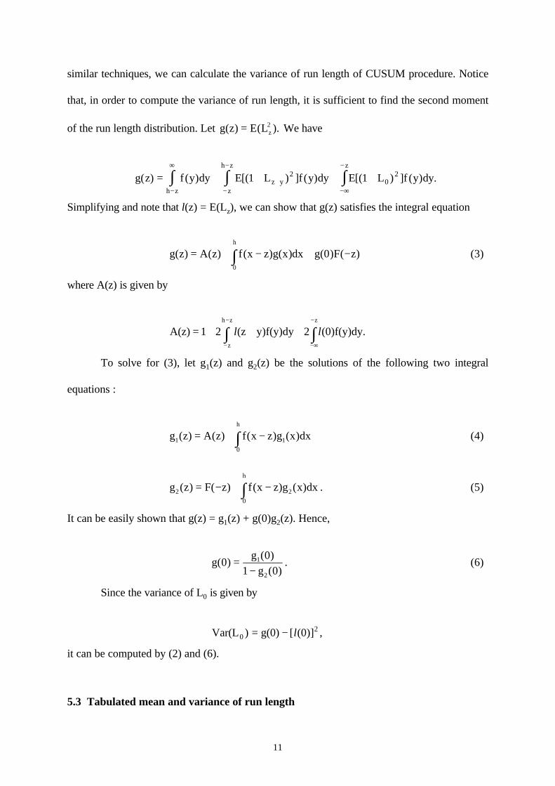
similar techniques, we can calculate the variance of run length of CUSUM procedure. Notice

that, in order to compute the variance of run length, it is sufficient to find the second moment

of the run length distribution. Let g(z E Lz) ( ).= 2 We have

g z f y dy E L f y dy E L f y dyz y

z

z

h z

h z

( ) ( ) [( ) ] ( ) [( ) ] ( ) .= + + + ++−∞

−

−

−

−

∞

∫∫∫ 1 120

2

Simplifying and note that l(z) = E(Lz), we can show that g(z) satisfies the integral equation

g(z A z f x z g(x dx g( F zh

) ( ) ( ) ) ) ( )= + − + −∫ 00

(3)

where A(z) is given by

A(z) 1 2 (z y)f(y)dy 2 (0)f(y)dy.z

z

h z

= + + +−∞

−

−

−

∫∫ l l

To solve for (3), let g1(z) and g2(z) be the solutions of the following two integral

equations :

g z A z f x z g x dxh

1 1

0

( ) ( ) ( ) ( )= + −∫ (4)

g z F z f x z g x dxh

2 2

0

( ) ( ) ( ) ( )= − + −∫ . (5)

It can be easily shown that g(z) = g1(z) + g(0)g2(z). Hence,

g(g

g0

01 0

1

2

)( )

( )=

−. (6)

Since the variance of L0 is given by

Var(L ) g(0) [ (0)]02= − l ,

it can be computed by (2) and (6).

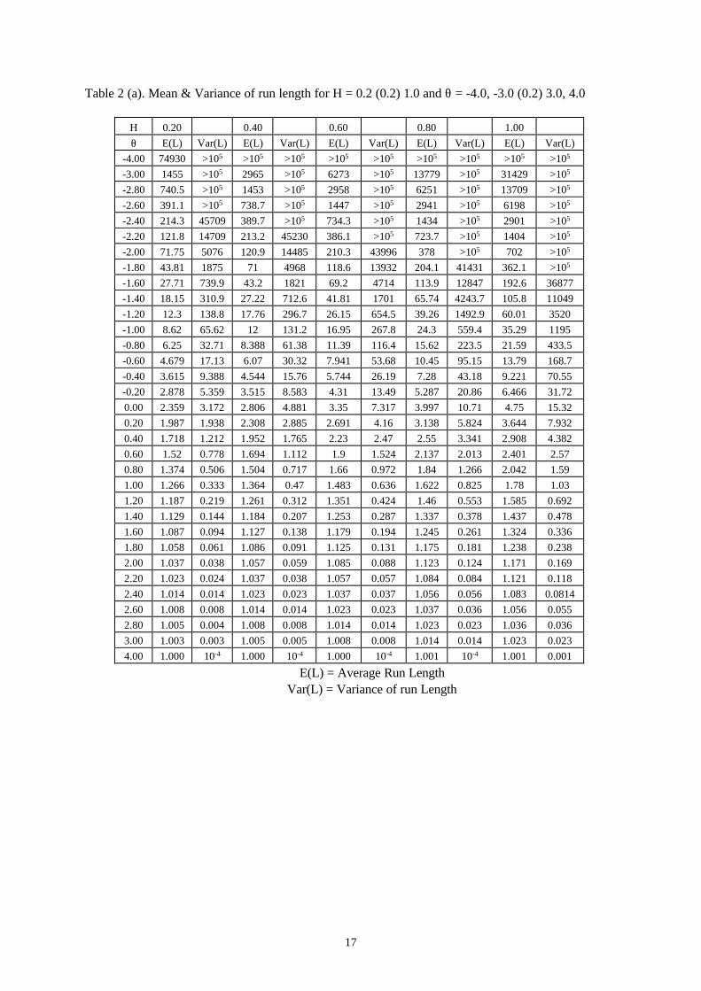
5.3 Tabulated mean and variance of run length

12

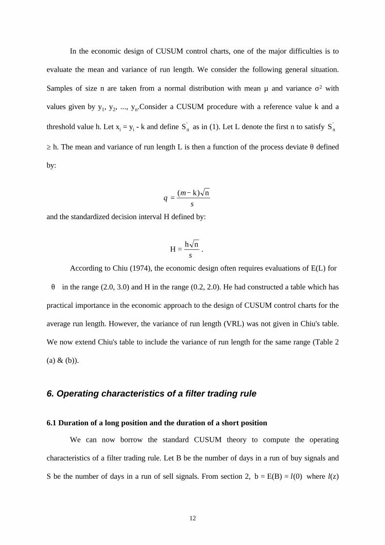
In the economic design of CUSUM control charts, one of the major difficulties is to

evaluate the mean and variance of run length. We consider the following general situation.

Samples of size n are taken from a normal distribution with mean µ and variance σ2 with

values given by y1, y2, ..., yn.Consider a CUSUM procedure with a reference value k and a

threshold value h. Let xi = yi - k and define Sn' as in (1). Let L denote the first n to satisfy Sn

'

≥ h. The mean and variance of run length L is then a function of the process deviate θ defined

by:

θµ

σ=

−( )k n

and the standardized decision interval H defined by:

Hh n

=σ

.

According to Chiu (1974), the economic design often requires evaluations of E(L) for

θ in the range (2.0, 3.0) and H in the range (0.2, 2.0). He had constructed a table which has

practical importance in the economic approach to the design of CUSUM control charts for the

average run length. However, the variance of run length (VRL) was not given in Chiu's table.

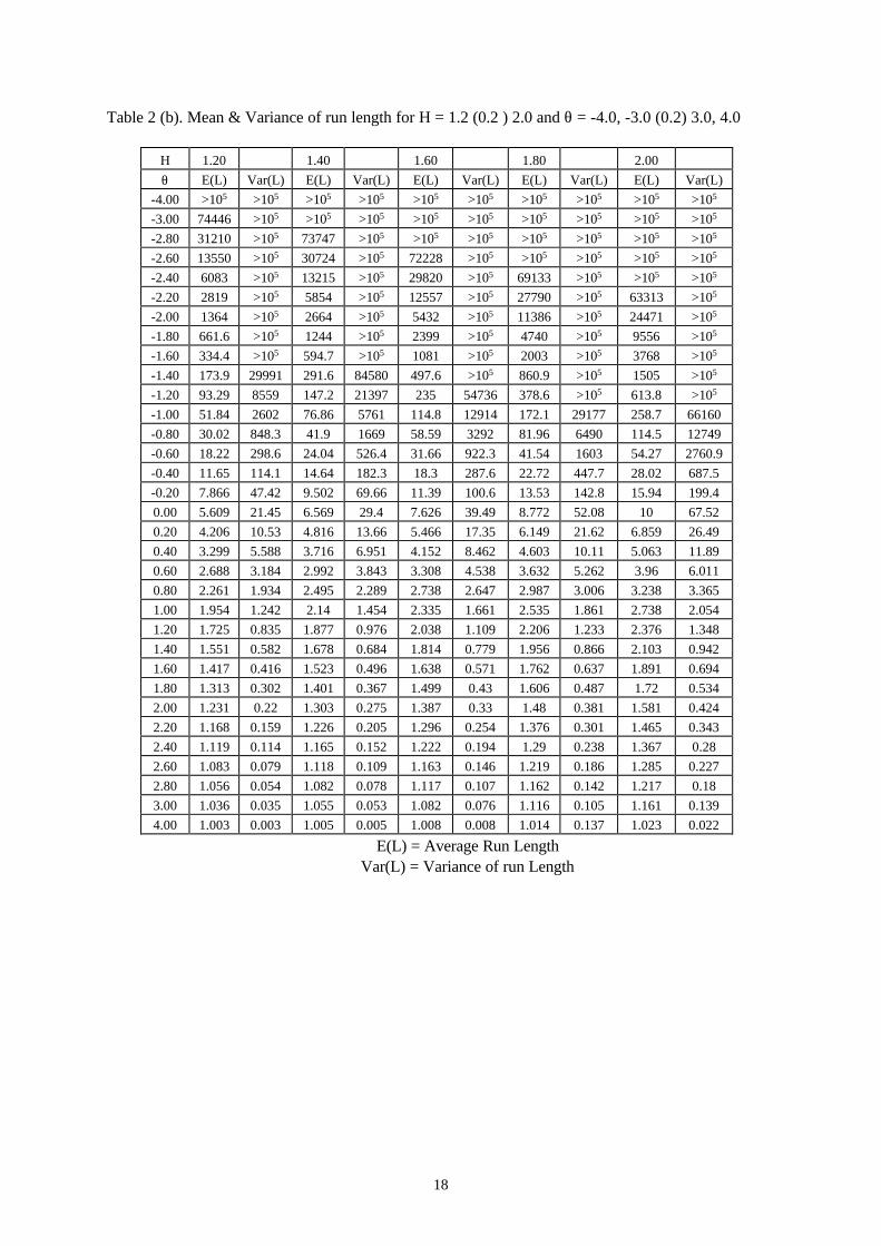
We now extend Chiu's table to include the variance of run length for the same range (Table 2

(a) & (b)).

6. Operating characteristics of a filter trading rule

6.1 Duration of a long position and the duration of a short position

We can now borrow the standard CUSUM theory to compute the operating

characteristics of a filter trading rule. Let B be the number of days in a run of buy signals and

S be the number of days in a run of sell signals. From section 2, b E(B) (0)= = l where l(z)

13

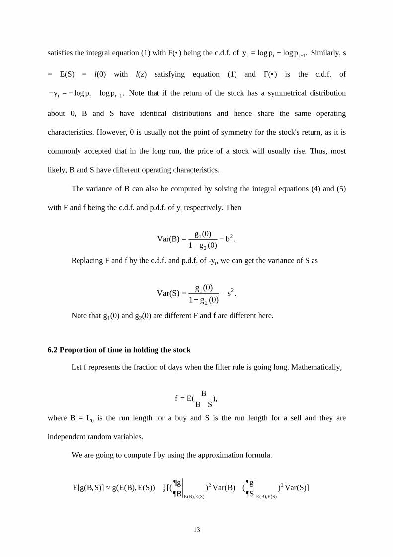
satisfies the integral equation (1) with F(•) being the c.d.f. of y p pt t t= − −log log .1 Similarly, s

= E(S) = l(0) with l(z) satisfying equation (1) and F(•) is the c.d.f. of

− = − + −y p pt t tlog log .1 Note that if the return of the stock has a symmetrical distribution

about 0, B and S have identical distributions and hence share the same operating

characteristics. However, 0 is usually not the point of symmetry for the stock's return, as it is

commonly accepted that in the long run, the price of a stock will usually rise. Thus, most

likely, B and S have different operating characteristics.

The variance of B can also be computed by solving the integral equations (4) and (5)

with F and f being the c.d.f. and p.d.f. of yt respectively. Then

Var(B)g (0)

1 g (0)b .1

2

2=−

−

Replacing F and f by the c.d.f. and p.d.f. of -yt, we can get the variance of S as

Var(S)g (0)

1 g (0)s .1

2

2=−

−

Note that g1(0) and g2(0) are different F and f are different here.

6.2 Proportion of time in holding the stock

Let f represents the fraction of days when the filter rule is going long. Mathematically,

f EB

B S=

+( ),

where B = L0 is the run length for a buy and S is the run length for a sell and they are

independent random variables.

We are going to compute f by using the approximation formula.

E g(B S g(E B E Sg

BVar B

g

SVar S

E B E S E B E S

[ , )] ( ), ( )) [( ) ( ) ( ) ( )]( ), ( ) ( ), ( )

≈ + +12

2 2∂∂

∂∂

14

Hence,

EB

B S

E B

E B E S E B E SE S Var B Var S( )

( )

( ) ( ) [ ( ) ( )]{[ ( )] ( ) ( )}

+≈

++

++

1

2 22 .

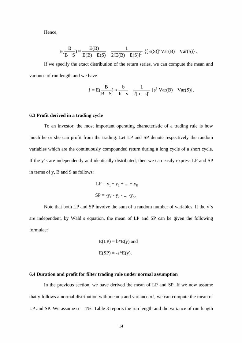
If we specify the exact distribution of the return series, we can compute the mean and

variance of run length and we have

f EB

B Sb

b s b ss B Var S=

+≈

++

++( )

[ ][ ( ) ( )]

12 2

2 Var .

6.3 Profit derived in a trading cycle

To an investor, the most important operating characteristic of a trading rule is how

much he or she can profit from the trading. Let LP and SP denote respectively the random

variables which are the continuously compounded return during a long cycle of a short cycle.

If the y’s are independently and identically distributed, then we can easily express LP and SP

in terms of y, B and S as follows:

LP = y1 + y2 + ... + yB

SP = -y1 - y2 - ... -yS.

Note that both LP and SP involve the sum of a random number of variables. If the y’s

are independent, by Wald’s equation, the mean of LP and SP can be given the following

formulae:

E(LP) = b*E(y) and

E(SP) = -s*E(y).

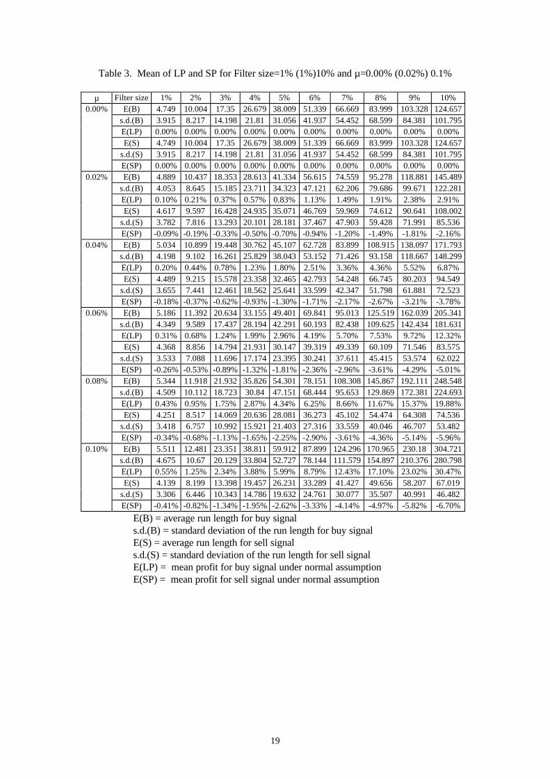
6.4 Duration and profit for filter trading rule under normal assumption

In the previous section, we have derived the mean of LP and SP. If we now assume

that y follows a normal distribution with mean µ and variance σ2, we can compute the mean of

LP and SP. We assume σ = 1%. Table 3 reports the run length and the variance of run length

15

for buy signal and sell signal. Furthermore, the mean of LP and SP are also reported.

7. Conclusion and DiscussionIn this paper, we find that there is a close relationship between the filter trading rule

and the CUSUM procedures used in the construction of industrial control charts. Applying

CUSUM techniques, we derive the mean and variance of the duration of a long position and

short position under filter trading rule. Furthermore, operating characteristics of the filter

trading profits have been constructed.

However, the ordinary filter trading rule is just the simplest case of CUSUM

techniques. Obviously, we can consider a general filter trading rule by using the general

version of CUSUM procedures. The generalized filter trading rule is compared with the

ordinary filter trading rule. Empirically, we find that the generalized filter trading rules have

satisfactory performance. This opens up the possibility of applying QC techniques to derive

technical trading rules in the financial market. The empirical results of applying the generalized

CUSUM techniques to technical trading are encouraging and further research along this

direction is suggested.

16

Table 1. Results on generalized filter trading rule.

h(%) h/k 10 20 30 40 50 ∞ -50 -40 -30 -20 -101 no. of cycle 577 610 622 630 635 645 664 669 672 685 711

Mean profit (%) 2.12 2.06 2.04 2.01 1.97 1.97 1.87 1.84 1.85 1.79 1.79s.d. profit (%) 6.90 6.66 6.63 6.62 6.57 6.52 6.41 6.39 6.35 6.29 6.16

Daily profit (%) -0.0288 -0.0366 -0.0393 -0.0435 -0.0474 -0.0490 -0.0615 -0.0653 -0.0650 -0.0729 -0.07672 no. of cycle 295 324 337 343 353 368 384 388 395 411 471


Daily profit (%) 0.0626 0.0599 0.0575 0.0626 0.0543 0.0514 0.0520 0.0526 0.0588 0.0482 0.01923 no. of cycle 171 206 218 225 231 246 266 272 282 301 356
















Daily profit (%) 0.0112 0.0343 0.0374 0.0762 0.0899 0.1144 0.0992 0.1082 0.1064 0.098 0.0370

where Mean profit = mean profit for each cycle for the filter trading rules s.d. profit = standard deviation of profit for each cycle for the filter trading rules no. of cycle = number of complete trading cycles Daily profit = daily profit for the filter trading rules.

17

Table 2 (a). Mean & Variance of run length for H = 0.2 (0.2) 1.0 and θ = -4.0, -3.0 (0.2) 3.0, 4.0

H 0.20 0.40 0.60 0.80 1.00

θ E(L) Var(L) E(L) Var(L) E(L) Var(L) E(L) Var(L) E(L) Var(L)

-4.00 74930 >105 >105 >105 >105 >105 >105 >105 >105 >105

-3.00 1455 >105 2965 >105 6273 >105 13779 >105 31429 >105

-2.80 740.5 >105 1453 >105 2958 >105 6251 >105 13709 >105

-2.60 391.1 >105 738.7 >105 1447 >105 2941 >105 6198 >105

-2.40 214.3 45709 389.7 >105 734.3 >105 1434 >105 2901 >105

-2.20 121.8 14709 213.2 45230 386.1 >105 723.7 >105 1404 >105

-2.00 71.75 5076 120.9 14485 210.3 43996 378 >105 702 >105

-1.80 43.81 1875 71 4968 118.6 13932 204.1 41431 362.1 >105

-1.60 27.71 739.9 43.2 1821 69.2 4714 113.9 12847 192.6 36877

-1.40 18.15 310.9 27.22 712.6 41.81 1701 65.74 4243.7 105.8 11049

-1.20 12.3 138.8 17.76 296.7 26.15 654.5 39.26 1492.9 60.01 3520

-1.00 8.62 65.62 12 131.2 16.95 267.8 24.3 559.4 35.29 1195

-0.80 6.25 32.71 8.388 61.38 11.39 116.4 15.62 223.5 21.59 433.5

-0.60 4.679 17.13 6.07 30.32 7.941 53.68 10.45 95.15 13.79 168.7

-0.40 3.615 9.388 4.544 15.76 5.744 26.19 7.28 43.18 9.221 70.55

-0.20 2.878 5.359 3.515 8.583 4.31 13.49 5.287 20.86 6.466 31.72

0.00 2.359 3.172 2.806 4.881 3.35 7.317 3.997 10.71 4.75 15.32

0.20 1.987 1.938 2.308 2.885 2.691 4.16 3.138 5.824 3.644 7.932

0.40 1.718 1.212 1.952 1.765 2.23 2.47 2.55 3.341 2.908 4.382

0.60 1.52 0.778 1.694 1.112 1.9 1.524 2.137 2.013 2.401 2.57

0.80 1.374 0.506 1.504 0.717 1.66 0.972 1.84 1.266 2.042 1.59

1.00 1.266 0.333 1.364 0.47 1.483 0.636 1.622 0.825 1.78 1.03

1.20 1.187 0.219 1.261 0.312 1.351 0.424 1.46 0.553 1.585 0.692

1.40 1.129 0.144 1.184 0.207 1.253 0.287 1.337 0.378 1.437 0.478

1.60 1.087 0.094 1.127 0.138 1.179 0.194 1.245 0.261 1.324 0.336

1.80 1.058 0.061 1.086 0.091 1.125 0.131 1.175 0.181 1.238 0.238

2.00 1.037 0.038 1.057 0.059 1.085 0.088 1.123 0.124 1.171 0.169

2.20 1.023 0.024 1.037 0.038 1.057 0.057 1.084 0.084 1.121 0.118

2.40 1.014 0.014 1.023 0.023 1.037 0.037 1.056 0.056 1.083 0.0814

2.60 1.008 0.008 1.014 0.014 1.023 0.023 1.037 0.036 1.056 0.055

2.80 1.005 0.004 1.008 0.008 1.014 0.014 1.023 0.023 1.036 0.036

3.00 1.003 0.003 1.005 0.005 1.008 0.008 1.014 0.014 1.023 0.023

4.00 1.000 10-4 1.000 10-4 1.000 10-4 1.001 10-4 1.001 0.001

E(L) = Average Run LengthVar(L) = Variance of run Length

18

Table 2 (b). Mean & Variance of run length for H = 1.2 (0.2 ) 2.0 and θ = -4.0, -3.0 (0.2) 3.0, 4.0

H 1.20 1.40 1.60 1.80 2.00

θ E(L) Var(L) E(L) Var(L) E(L) Var(L) E(L) Var(L) E(L) Var(L)

-4.00 >105 >105 >105 >105 >105 >105 >105 >105 >105 >105

-3.00 74446 >105 >105 >105 >105 >105 >105 >105 >105 >105

-2.80 31210 >105 73747 >105 >105 >105 >105 >105 >105 >105

-2.60 13550 >105 30724 >105 72228 >105 >105 >105 >105 >105

-2.40 6083 >105 13215 >105 29820 >105 69133 >105 >105 >105

-2.20 2819 >105 5854 >105 12557 >105 27790 >105 63313 >105

-2.00 1364 >105 2664 >105 5432 >105 11386 >105 24471 >105

-1.80 661.6 >105 1244 >105 2399 >105 4740 >105 9556 >105

-1.60 334.4 >105 594.7 >105 1081 >105 2003 >105 3768 >105

-1.40 173.9 29991 291.6 84580 497.6 >105 860.9 >105 1505 >105

-1.20 93.29 8559 147.2 21397 235 54736 378.6 >105 613.8 >105

-1.00 51.84 2602 76.86 5761 114.8 12914 172.1 29177 258.7 66160

-0.80 30.02 848.3 41.9 1669 58.59 3292 81.96 6490 114.5 12749

-0.60 18.22 298.6 24.04 526.4 31.66 922.3 41.54 1603 54.27 2760.9

-0.40 11.65 114.1 14.64 182.3 18.3 287.6 22.72 447.7 28.02 687.5

-0.20 7.866 47.42 9.502 69.66 11.39 100.6 13.53 142.8 15.94 199.4

0.00 5.609 21.45 6.569 29.4 7.626 39.49 8.772 52.08 10 67.52

0.20 4.206 10.53 4.816 13.66 5.466 17.35 6.149 21.62 6.859 26.49

0.40 3.299 5.588 3.716 6.951 4.152 8.462 4.603 10.11 5.063 11.89

0.60 2.688 3.184 2.992 3.843 3.308 4.538 3.632 5.262 3.96 6.011

0.80 2.261 1.934 2.495 2.289 2.738 2.647 2.987 3.006 3.238 3.365

1.00 1.954 1.242 2.14 1.454 2.335 1.661 2.535 1.861 2.738 2.054

1.20 1.725 0.835 1.877 0.976 2.038 1.109 2.206 1.233 2.376 1.348

1.40 1.551 0.582 1.678 0.684 1.814 0.779 1.956 0.866 2.103 0.942

1.60 1.417 0.416 1.523 0.496 1.638 0.571 1.762 0.637 1.891 0.694

1.80 1.313 0.302 1.401 0.367 1.499 0.43 1.606 0.487 1.72 0.534

2.00 1.231 0.22 1.303 0.275 1.387 0.33 1.48 0.381 1.581 0.424

2.20 1.168 0.159 1.226 0.205 1.296 0.254 1.376 0.301 1.465 0.343

2.40 1.119 0.114 1.165 0.152 1.222 0.194 1.29 0.238 1.367 0.28

2.60 1.083 0.079 1.118 0.109 1.163 0.146 1.219 0.186 1.285 0.227

2.80 1.056 0.054 1.082 0.078 1.117 0.107 1.162 0.142 1.217 0.18

3.00 1.036 0.035 1.055 0.053 1.082 0.076 1.116 0.105 1.161 0.139

4.00 1.003 0.003 1.005 0.005 1.008 0.008 1.014 0.137 1.023 0.022

E(L) = Average Run LengthVar(L) = Variance of run Length

19

Table 3. Mean of LP and SP for Filter size=1% (1%)10% and µ=0.00% (0.02%) 0.1%

µ Filter size 1% 2% 3% 4% 5% 6% 7% 8% 9% 10%0.00% E(B) 4.749 10.004 17.35 26.679 38.009 51.339 66.669 83.999 103.328 124.657

s.d.(B) 3.915 8.217 14.198 21.81 31.056 41.937 54.452 68.599 84.381 101.795E(LP) 0.00% 0.00% 0.00% 0.00% 0.00% 0.00% 0.00% 0.00% 0.00% 0.00%E(S) 4.749 10.004 17.35 26.679 38.009 51.339 66.669 83.999 103.328 124.657

s.d.(S) 3.915 8.217 14.198 21.81 31.056 41.937 54.452 68.599 84.381 101.795E(SP) 0.00% 0.00% 0.00% 0.00% 0.00% 0.00% 0.00% 0.00% 0.00% 0.00%

0.02% E(B) 4.889 10.437 18.353 28.613 41.334 56.615 74.559 95.278 118.881 145.489s.d.(B) 4.053 8.645 15.185 23.711 34.323 47.121 62.206 79.686 99.671 122.281E(LP) 0.10% 0.21% 0.37% 0.57% 0.83% 1.13% 1.49% 1.91% 2.38% 2.91%E(S) 4.617 9.597 16.428 24.935 35.071 46.769 59.969 74.612 90.641 108.002

s.d.(S) 3.782 7.816 13.293 20.101 28.181 37.467 47.903 59.428 71.991 85.536E(SP) -0.09% -0.19% -0.33% -0.50% -0.70% -0.94% -1.20% -1.49% -1.81% -2.16%

0.04% E(B) 5.034 10.899 19.448 30.762 45.107 62.728 83.899 108.915 138.097 171.793s.d.(B) 4.198 9.102 16.261 25.829 38.043 53.152 71.426 93.158 118.667 148.299E(LP) 0.20% 0.44% 0.78% 1.23% 1.80% 2.51% 3.36% 4.36% 5.52% 6.87%E(S) 4.489 9.215 15.578 23.358 32.465 42.793 54.248 66.745 80.203 94.549

s.d.(S) 3.655 7.441 12.461 18.562 25.641 33.599 42.347 51.798 61.881 72.523E(SP) -0.18% -0.37% -0.62% -0.93% -1.30% -1.71% -2.17% -2.67% -3.21% -3.78%

0.06% E(B) 5.186 11.392 20.634 33.155 49.401 69.841 95.013 125.519 162.039 205.341s.d.(B) 4.349 9.589 17.437 28.194 42.291 60.193 82.438 109.625 142.434 181.631E(LP) 0.31% 0.68% 1.24% 1.99% 2.96% 4.19% 5.70% 7.53% 9.72% 12.32%E(S) 4.368 8.856 14.794 21.931 30.147 39.319 49.339 60.109 71.546 83.575

s.d.(S) 3.533 7.088 11.696 17.174 23.395 30.241 37.611 45.415 53.574 62.022E(SP) -0.26% -0.53% -0.89% -1.32% -1.81% -2.36% -2.96% -3.61% -4.29% -5.01%

0.08% E(B) 5.344 11.918 21.932 35.826 54.301 78.151 108.308 145.867 192.111 248.548s.d.(B) 4.509 10.112 18.723 30.84 47.151 68.444 95.653 129.869 172.381 224.693E(LP) 0.43% 0.95% 1.75% 2.87% 4.34% 6.25% 8.66% 11.67% 15.37% 19.88%E(S) 4.251 8.517 14.069 20.636 28.081 36.273 45.102 54.474 64.308 74.536

s.d.(S) 3.418 6.757 10.992 15.921 21.403 27.316 33.559 40.046 46.707 53.482E(SP) -0.34% -0.68% -1.13% -1.65% -2.25% -2.90% -3.61% -4.36% -5.14% -5.96%

0.10% E(B) 5.511 12.481 23.351 38.811 59.912 87.899 124.296 170.965 230.18 304.721s.d.(B) 4.675 10.67 20.129 33.804 52.727 78.144 111.579 154.897 210.376 280.798E(LP) 0.55% 1.25% 2.34% 3.88% 5.99% 8.79% 12.43% 17.10% 23.02% 30.47%E(S) 4.139 8.199 13.398 19.457 26.231 33.289 41.427 49.656 58.207 67.019

s.d.(S) 3.306 6.446 10.343 14.786 19.632 24.761 30.077 35.507 40.991 46.482E(SP) -0.41% -0.82% -1.34% -1.95% -2.62% -3.33% -4.14% -4.97% -5.82% -6.70%

E(B) = average run length for buy signals.d.(B) = standard deviation of the run length for buy signalE(S) = average run length for sell signals.d.(S) = standard deviation of the run length for sell signalE(LP) = mean profit for buy signal under normal assumptionE(SP) = mean profit for sell signal under normal assumption

20

REFERENCES

ALEXANDER, S. (1961) Price Movements in Speculative Markets: Trends or Random Walk,

Industrial Management Review, 2, pp.7-26.

ALEXANDER, S. (1964) Price Movements in Speculative Markets: Trends or Random Walk, No.

2, Industrial Management Review, 5, pp.338-372.

CHIU, W. K. (1974) The Economic Design of CUSUM Charts for Controlling Normal Means,

Applied Statistics, 23,pp.420-433.

CROWDER, S. V. (1987) A Simple Method for Studying Run-Length Distributions of

Exponentially Weighted Moving Average Charts, Technometrics, 29, No.4, pp.401-407.

FAMA, E. & BLUME, M. (1966) Filter Rules and Stock Market Trading, Journal of Business,

40, pp.226-241.

FAMA, E. (1970) Efficient Capital Markets: A review of Theory and Empirical Work, Journal

of Finance, 25, pp.383-417.

GOEL, A. L. & WU, S. M. (1971) Determination of A.R.L. and a Contour Nomogram for

CUSUM Charts to Control Normal Mean, Technometrics, 13, No.2, pp.221-230.

JEGADEESH, N. and TITMAN, S. (1993) Return to buying winners and selling losers: Implications

for stock market efficiency, Journal of Finance, pp.65-91.

KANTOROVICH, L. V. & KRYLOV, V. I. (1958) Approximate Methods of Higher Analysis,

(Interscience Publishers, New York).

KEMP, K, W. (1961) The average run length of a cumulative sum chart when V-mask is used,

Journal of Royal Statistics Society B, 23, pp.149-153.

KEMP, K, W. (1962) The use of cumulative sums for sampling inspection schemes, Applied

Statistics, 11, pp.16-31.

LO, A., and MACKINLEY, A. C. (1988) Stock market prices do not follow random walks:

21

Evidence from a simple specification test, Review of Financial Studies 1, pp.41-66.

PAGE, E. S. (1954) Continuous Inspection Schemes, Biometrika, 41, pp.100-114.

PAGE, E. S. (1954) An improvement to Wald's approximation for some properties of

sequential tests, Journal of Royal Statistics Society B, 16, pp.136-139.

PRAETZ, Peter D. (1976) Rates of Return on Filter Tests, Journal of Finance, 31, pp.71-75.

PRAETZ, Peter D. (1979) A General Test of a Filter Effect, Journal of Financial and

Quantitative Analysis, 14, pp.385-394.

VAN DOBBEN DE BRUYN, C. S. (1968) Cumulative Sums tests: Theory and Practice, (Hafner

Publishing Company, New York).

cusum techniques for technical trading in financial market · cusum techniques for technical...

Documents