copyright by berkay kocababuc 2011
TRANSCRIPT

Copyright
by
Berkay Kocababuc
2011
The Thesis Committee for Berkay Kocababuc
Certifies that this is the approved version of the following thesis:
Finite Element Analysis of Wellbore Strengthening
APPROVED BY
SUPERVISING COMMITTEE:
Kenneth E. Gray
Evgeny Podnos
Supervisor:
Co-Supervisor:
Finite Element Analysis of Wellbore Strengthening
by
Berkay Kocababuc, B.S.
Thesis
Presented to the Faculty of the Graduate School of
The University of Texas at Austin
in Partial Fulfillment
of the Requirements
for the Degree of
Master of Science in Engineering
The University of Texas at Austin
December 2011

Dedication
To my father.

v
Acknowledgements
First and foremost, I would like to express my deepest gratitude to my supervisor,
Dr. Kenneth Gray for his guidance and encouragement on the project. His endless
patience and support resulted in the final product of this study.
I would also like to thank Dr. Eric Becker and Dr. Evgeny Podnos for taking the
time to provide valuable feedback and knowledge. This thesis would not have been
possible without their help and suggestions.
I want to offer my deepest gratitude to Dr. Paul Bommer for giving me the
opportunity to work as a teaching assistant in Blowout Prevention and Control course. It
was a valuable experience.
I’m also very thankful to Turkish Petroleum Corporation for their financial
support.
Finally, I’m very grateful to my family for their love, encouragement and support.
I would not have been able to accomplish any of this without them.
December 2, 2011

vi
Abstract
Finite Element Analysis of Wellbore Strengthening
Berkay Kocababuc, M.S.E
The University of Texas at Austin, 2011
Supervisor: Kenneth E. Gray
Co-Supervisor: Evgeny Podnos
As the world energy demand increases, drilling deeper wells is inevitable. Deeper
wells have abnormal pressure zones where the difference between pore pressure and
fracture pressure gradient, is very small. Smaller drilling margins make it harder to drill
the well and result in high operation costs due to the increase of non-productive time.
One of the major factors influence non-productive time in drilling operations is lost
circulation due to drilling induced fractures. The most common approach is still plugging
the fractures by using various loss circulation materials and there are several wellbore
strengthening techniques present in the literature to explain the physics behind this
treatment. This thesis focuses on development of a rock mechanics/hydraulic model for
quantifying the stress distribution around the wellbore and fracture geometry after
fracture initiation, propagation and plugging the fracture with loss circulation materials.
In addition, fracture behavior is investigated in different stress states, for different
vii
permeability values and in the presence of multiple fractures. The following chapters
contain detailed description of this model, and analysis results.

viii
Table of Contents
List of Tables ......................................................................................................... ix
List of Figures ..........................................................................................................x
1. Introduction .....................................................................................................1
1.1. Lost Circulation .....................................................................................2
1.2. Drilling Induced Fractures .....................................................................3
1.3. Wellbore Strengthening .........................................................................6
2. Finite Element Analysis of Wellbore Strengthening ......................................7
2.1. Two-Dimensional Model Description ...................................................7
2.1.1. Geometry of the Model ........................................................7
2.1.2. Accuracy of the Model and Mesh ........................................9
2.1.3. Fracture Modeling ..............................................................13
2.1.4. Multiple Fractures ..............................................................15
2.2. Three-Dimensional Model Description ...............................................16
2.2.1. Geometry of the Model ......................................................16
2.2.2. Initial and Boundary Conditions ........................................17
2.2.3. Accuracy of the Model and Mesh ......................................18
2.2.4. Fracture Modeling ..............................................................21
2.2.4.1. Mechanical Behavior of the Fracture Zone .................21
2.2.4.2. Pore Fluid Flow Properties at the Fracture Zone ........23
3. Results ...........................................................................................................25
3.1. Two-Dimensional Analysis of Wellbore Strengthening ......................25
3.2. Three-Dimensional Analysis of Wellbore Strengthening ....................39
4. Conclusions ...................................................................................................48
References ..............................................................................................................50
ix
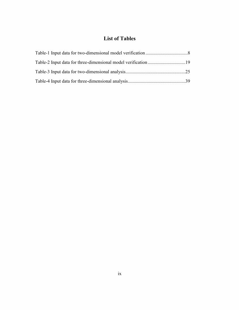
List of Tables
Table-1 Input data for two-dimensional model verification ....................................8
Table-2 Input data for three-dimensional model verification ................................19
Table-3 Input data for two-dimensional analysis ...................................................25
Table-4 Input data for three-dimensional analysis .................................................39
x
List of Figures
Figure-1.1. Problem incidents, Gulf of Mexico shelf gas wells (Grayson 2009) ....2
Figure-1.2. Stress states superposition for equal horizontal stresses (Hubert, M.K. and
Willis, D.G. 1957) ...............................................................................3
Figure-1.3. Stress fields for different horizontal stress ratios (Hubert, M.K. and
Willis, D.G. 1957) ...............................................................................4
Figure-1.4. Stress states superposition with wellbore pressure (Hubert, M.K. and
Willis, D.G. 1957) ...............................................................................5
Figure-2.1. Two-dimensional model geometry .......................................................7
Figure-2.2. Boundary conditions of the two-dimensional model ............................8
Figure-2.3. Quad shape elements with different geometric orders ..........................9
Figure-2.4. Mesh with different element densities ................................................10
Figure-2.5. Hoop stress distribution around the wellbore for different number of
elements ............................................................................................10
Figure-2.6. Hoop stress for different geometric order ...........................................11
Figure-2.7. Hoop Stress Error for Four Node Quad Elements ..............................12
Figure-2.8. Hoop stress error for different geometric order ..................................12
Figure-2.9. Hoop stress distribution with a fracture ..............................................13
Figure-2.10. Hoop stress distribution with a bridge at the fracture mouth ............14
Figure-2.11. Multiple fractures around the wellbore .............................................15
Figure-2.12. Three-dimensional model loads ........................................................16
Figure-2.13. Boundary conditions of the three-dimensional model ......................17
Figure-2.14. Hex shape elements with different geometric orders (Abaqus 6.10-EF
Documentation, 2010).......................................................................19
xi
Figure-2.15. Three-dimensional model mesh ........................................................20
Figure-2.16. Hoop stress distribution for different geometric order and mesh .....20
Figure-2.17. Three-dimensional cohesive element (Abaqus 6.10 Documentation,
2010) .................................................................................................21
Figure-2.18. Flow patterns of pore fluid within cohesive elements (Abaqus 6.10-EF
Documentation, 2010).......................................................................23
Figure-2.19. Permeable layers of a cohesive element ............................................23
Figure-3.1. Hoop stress distribution with zero wellbore pressure .........................26
Figure-3.2. Hoop stress distribution with initiation pressure applied to the wellbore
...........................................................................................................26
Figure-3.3. Radial stress distribution with zero wellbore pressure ........................27
Figure-3.4. Radial stress distribution with initiation pressure applied to the wellbore
...........................................................................................................27
Figure-3.5. Hoop stress change along the wellbore ...............................................28
Figure-3.6. Radial stress change along the wellbore .............................................28
Figure-3.7. Hoop stress distribution after fracture propagation (deformations
magnified 20 times) ..........................................................................29
Figure-3.8. Hoop stress distribution after plugging (deformations magnified 20 times)
...........................................................................................................30
Figure-3.9. Change in fracture opening after plugging..........................................31
Figure-3.10. Hoop stress distribution with initiation pressure applied to the wellbore
...........................................................................................................31
Figure-3.11. Hoop stress distribution with a lower wellbore pressure ..................31
Figure-3.12. Fracture opening for different wellbore pressures ............................32
Figure-3.13. Effects of stress anisotropy on fracture opening ...............................33

xii
Figure-3.14. Effects of stress anisotropy on hoop stress .......................................33
Figure-3.15. Hoop stress distribution after three fractures propagated (deformations
magnified 20 times) ..........................................................................34
Figure-3.16. Fracture lengths in multi fracture model ...........................................35
Figure-3.17. Fracture width comparison between single and multi fracture models35
Figure-3.18. Hoop stress distribution after plugging the primary fracture in multi
fractured model .................................................................................36
Figure-3.19. Change in primary fracture opening in multi fracture model ...........37
Figure-3.20. Change in secondary fracture opening in multi fracture model ........37
Figure-3.21. Hoop stress distribution for multi fracture model .............................38
Figure-3.22. Comparison of hoop stress increase between two models ................38
Figure-3.23. Hoop stress distribution at the end of first step in three-dimensional
model.................................................................................................40
Figure-3.24. Hoop stress distribution after fracture propagation in three-dimensional
model (deformation magnified 50 times) .........................................40
Figure-3.25. Hoop stress distribution after plugging the fracture in three-dimensional
model (deformation magnified 50 times) .........................................41
Figure-3.26. Fracture geometry in three-dimensional model ................................41
Figure-3.27. Hoop stress distributions during wellbore strengthening in three-
dimensional model ............................................................................42
Figure-3.28. Fracture geometry for different loss rates .........................................43
Figure-3.29. Hoop stress distribution after fracture propagation for different loss rates
...........................................................................................................44
Figure-3.30. Hoop stress distribution after plugging for different loss rates .........44
Figure-3.31. Effects of permeability on fracture growth .......................................45

xiii
Figure-3.32. Effects of permeability on hoop stress ..............................................45
Figure-3.33. Effects of mud cake permeability on fracture growth .......................46
Figure-3.34. Pore pressure distribution after fracture propagation ........................47

1
1. Introduction
In a drilling process, it is crucial to keep hydrostatic pressure gradient of the
drilling fluid in between pore pressure and fracture pressure gradients. When the
hydrostatic pressure of the drilling fluid is lower than the formation pore pressure at any
zone, formation fluid begins to flow into the wellbore. This influx can lead to a blowout
if it is not controlled. On the other hand, when the hydrostatic pressure of the drilling
fluid is higher than the fracture pressure, drilling fluid begins to flow into the formation
through drilling induced fractures. The flow of the drilling fluid into the formation
through drilling induced fractures can cause significant mud losses. To prevent influx and
mud losses, upper and lower limits of the operational hydrostatic pressure gradient of the
drilling fluid are defined by fracture pressure and pore pressure gradients. This margin,
between pore pressure and fracture pressure gradients, is known as mud-weight window.
Abnormalities in pressure zones result in smaller drilling margins. When the drilling
margin is small, it is harder to maintain drilling fluid gradient at desired levels which
increases the operation costs due to the increase of non-productive time. In addition, non-
productive time influences total drilling costs a lot more in deeper wells because daily
operating costs of deeper wells are much higher than shallower ones. According to the
data from James K. Dodson Company, average non-productive time for more than 1700
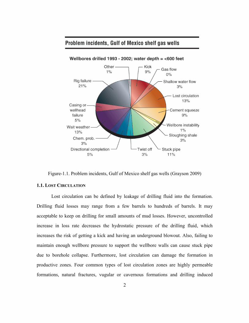
wells drilled between 1993 and 2002 in the Gulf of Mexico is 24% of the total drilling
time and 13% of the non-productive time caused by lost circulation (Grayson 2009).
2
Figure-1.1. Problem incidents, Gulf of Mexico shelf gas wells (Grayson 2009)
1.1. LOST CIRCULATION
Lost circulation can be defined by leakage of drilling fluid into the formation.
Drilling fluid losses may range from a few barrels to hundreds of barrels. It may
acceptable to keep on drilling for small amounts of mud losses. However, uncontrolled
increase in loss rate decreases the hydrostatic pressure of the drilling fluid, which
increases the risk of getting a kick and having an underground blowout. Also, failing to
maintain enough wellbore pressure to support the wellbore walls can cause stuck pipe
due to borehole collapse. Furthermore, lost circulation can damage the formation in
productive zones. Four common types of lost circulation zones are highly permeable
formations, natural fractures, vugular or cavernous formations and drilling induced

3
fractures. Seepage losses mostly occur at highly permeable formations located at shallow
depths. The fluid loss property of the mud cake has significant importance during
penetration of these highly permeable zones. Deeper formation matrices do not allow
fluid flow easily because they have lower permeability values compared to shallow zones
due to the overburden. However, severe lost circulation usually occurs through fractures
in deeper formations and the most common type of lost circulation is caused by induced
vertical fractures (Messenger, J. U. et al. 1981). In addition, 90% of the loss circulation
incidents are caused by fracture propagation (Dupriest 2005).
1.2.DRILLING INDUCED FRACTURES
Drilling induced fractures are tensile fractures which initiate when the tension due
to wellbore pressure exceeds the compressive stresses around the wellbore wall. Based on
the Kirsch solution, for an isotropic stress state in an infinite plate with a circular opening
tangential stress, which is often called hoop stress, is equal to two times to the horizontal
stress (Hubert, M.K. and Willis, D.G. 1957).
Figure-1.2. Stress states superposition for equal horizontal stresses (Hubert, M.K. and
Willis, D.G. 1957)
4
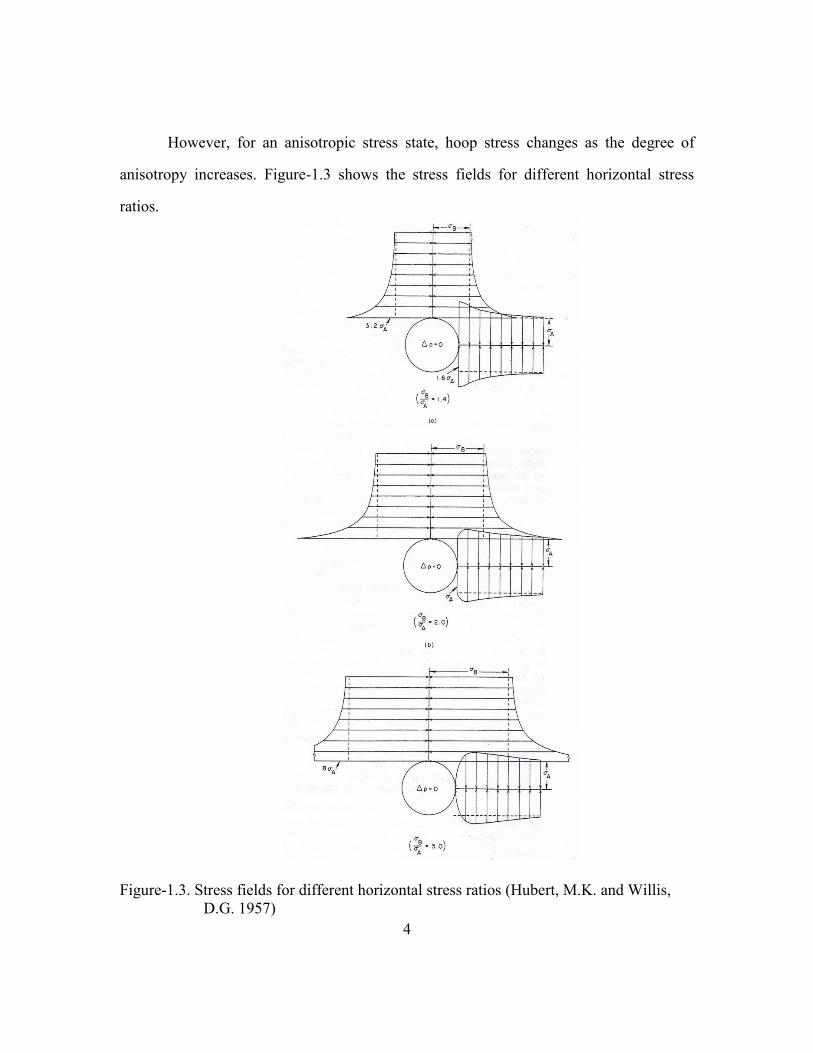
However, for an anisotropic stress state, hoop stress changes as the degree of
anisotropy increases. Figure-1.3 shows the stress fields for different horizontal stress
ratios.
Figure-1.3. Stress fields for different horizontal stress ratios (Hubert, M.K. and Willis,
D.G. 1957)
5
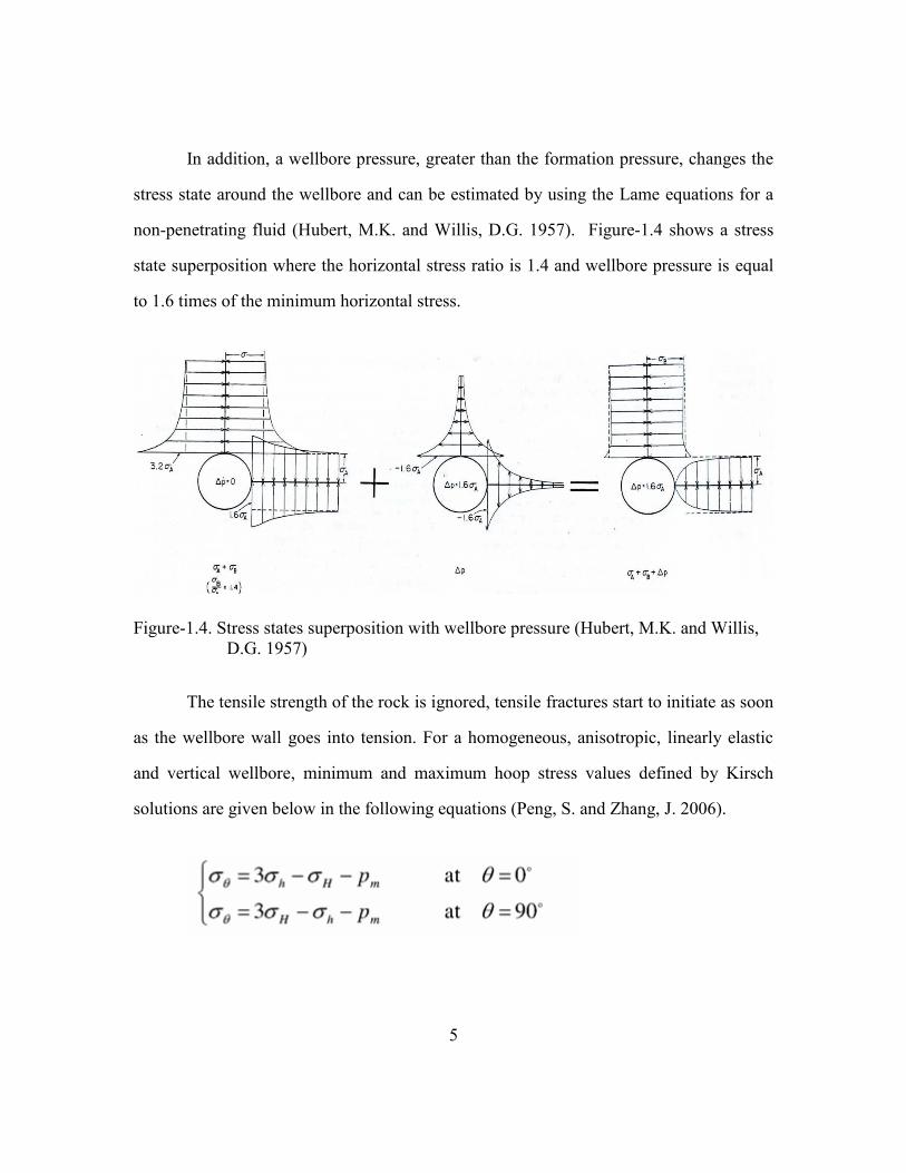
In addition, a wellbore pressure, greater than the formation pressure, changes the
stress state around the wellbore and can be estimated by using the Lame equations for a
non-penetrating fluid (Hubert, M.K. and Willis, D.G. 1957). Figure-1.4 shows a stress
state superposition where the horizontal stress ratio is 1.4 and wellbore pressure is equal
to 1.6 times of the minimum horizontal stress.
Figure-1.4. Stress states superposition with wellbore pressure (Hubert, M.K. and Willis,
D.G. 1957)
The tensile strength of the rock is ignored, tensile fractures start to initiate as soon
as the wellbore wall goes into tension. For a homogeneous, anisotropic, linearly elastic
and vertical wellbore, minimum and maximum hoop stress values defined by Kirsch
solutions are given below in the following equations (Peng, S. and Zhang, J. 2006).
6
1.3.WELLBORE STRENGTHENING
Wellbore Strengthening can be defined as increasing the resistance of the
formation to initiation or propagation of a fracture to obtain a wider mud window. There
are different techniques in the literature to strengthen a wellbore. Generally, wellbore
strengthening methods are either based on near wellbore region stress field alteration or
enhancing fracture propagation pressure by isolating the fracture tip (Van Oort et al.,
2009). The concepts “Stress Caging” and “Fracture Closure Stress” are two examples for
the wellbore strengthening methods based on near wellbore region stress field alteration
(Alberty and Mclean, 2004, Dupriest, 2005). Stress caging aims to plug the fracture
mouth with certain size materials to increase the tangential stress around the borehole
(Alberty and Mclean, 2004). In addition, the fracture closure stress method focuses on
fracture opening maximization and maintaining the width by filling the fractures with
wellbore strengthening materials where size of the particles is not important (Dupriest,
2005). On the other hand, “Fracture Propagation Resistance” is built on the pressure felt
at the fracture tip, which is the driving mechanism of fracture propagation, and it is
defined as extension of drilling margin by isolating fracture tip (Van Oort et al., 2009).
However, there will be no increase in fracture gradient; it can only stop propagation of an
existing fracture. In spite of successful field results reported for different approaches,
industry hasn’t found a common ground on factors effecting wellbore strengthening.
In the following chapters, a finite element model will be explained and simulation
results will be interpreted based on these approaches to identify which factors have the
most significant effect on wellbore strengthening. These factors can lead to design of the
best treatment for strengthening a wellbore.
7
2. Finite Element Analysis of Wellbore Strengthening
2.1.TWO-DIMENSIONAL MODEL DESCRIPTION
2.1.1. Geometry of the Model
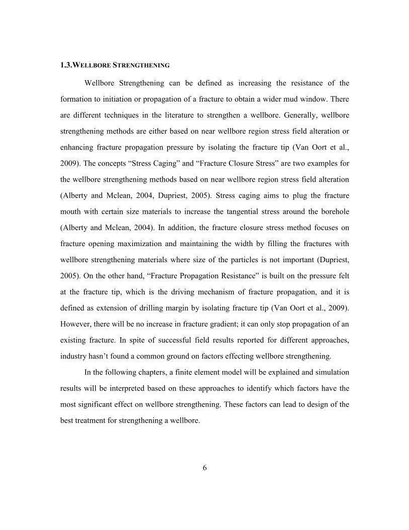
The model is constructed in two dimensions with plane strain elements by using
ABAQUS software. Only half of the wellbore is modeled due to symmetry. Length and
width of the model is shown in Figure-2.1.
Figure-2.1. Two-dimensional model geometry
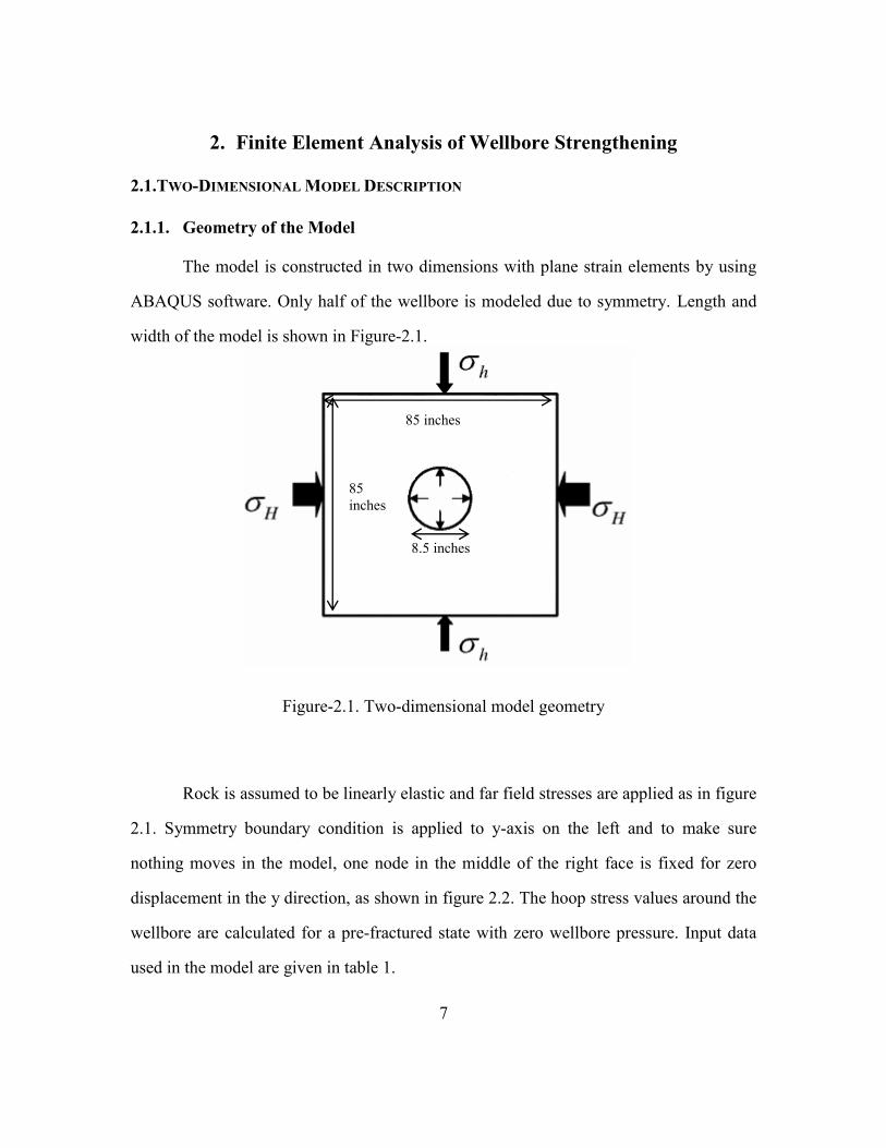
Rock is assumed to be linearly elastic and far field stresses are applied as in figure
2.1. Symmetry boundary condition is applied to y-axis on the left and to make sure
nothing moves in the model, one node in the middle of the right face is fixed for zero
displacement in the y direction, as shown in figure 2.2. The hoop stress values around the
wellbore are calculated for a pre-fractured state with zero wellbore pressure. Input data
used in the model are given in table 1.
85 inches
85
inches
8.5 inches
8
Figure-2.2. Boundary conditions of the two-dimensional model
Table-1 Input data for two-dimensional model verification
Wellbore diameter 8.5 inch
Max Horizontal Stress 2200 psi
Min Horizontal Stress 1800 psi
Young Modulus 1740000 psi
Poisson’s ratio 0.25
Displacement
of this node is
zero in y
direction
Symmetry
boundary
condition
9
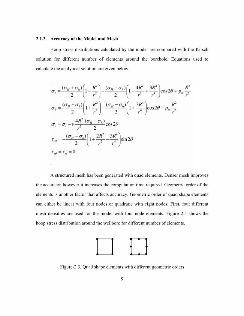
2.1.2. Accuracy of the Model and Mesh
Hoop stress distributions calculated by the model are compared with the Kirsch
solution for different number of elements around the borehole. Equations used to
calculate the analytical solution are given below.
A structured mesh has been generated with quad elements. Denser mesh improves
the accuracy; however it increases the computation time required. Geometric order of the
elements is another factor that affects accuracy. Geometric order of quad shape elements
can either be linear with four nodes or quadratic with eight nodes. First, four different
mesh densities are used for the model with four node elements. Figure 2.5 shows the
hoop stress distribution around the wellbore for different number of elements.
Figure-2.3. Quad shape elements with different geometric orders

10
Figure-2.4. Mesh with different element densities
Figure-2.5. Hoop stress distribution around the wellbore for different number of elements
2000
2500
3000
3500
4000
4500
5000
0 20 40 60 80 100
Ho
op
Str
ess
(p
si)
Angle (deg)
2D model with 4 node quad elements
Kirsch solution
160 elements around thehalf wellbore
120 elements around thehalf wellbore
80 elements around the halfwellbore
40 elements around the halfwellbore
11
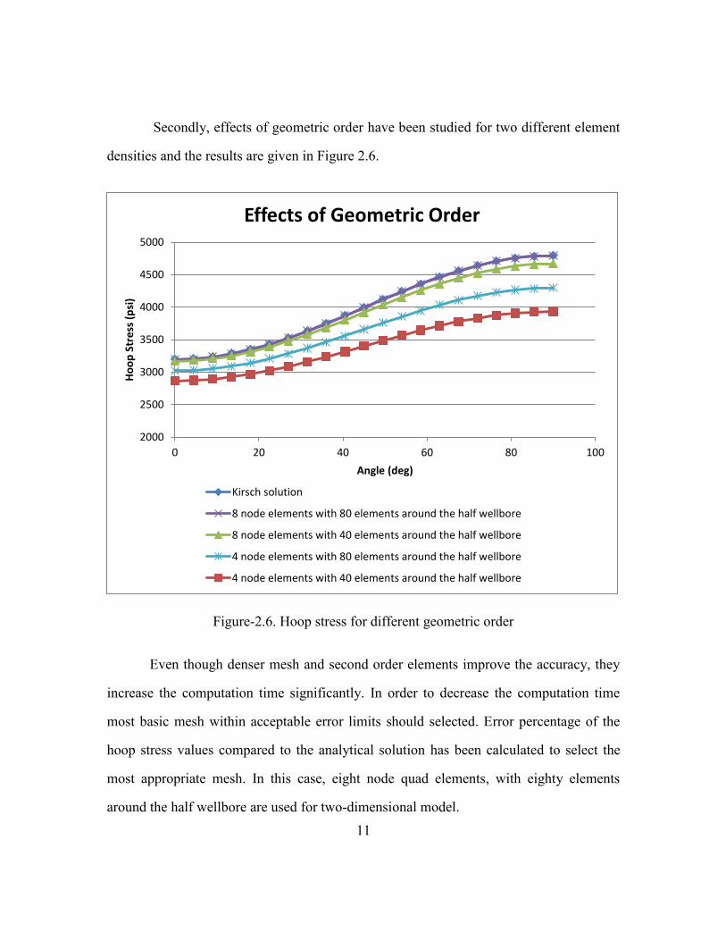
Secondly, effects of geometric order have been studied for two different element
densities and the results are given in Figure 2.6.
Figure-2.6. Hoop stress for different geometric order
Even though denser mesh and second order elements improve the accuracy, they
increase the computation time significantly. In order to decrease the computation time
most basic mesh within acceptable error limits should selected. Error percentage of the
hoop stress values compared to the analytical solution has been calculated to select the
most appropriate mesh. In this case, eight node quad elements, with eighty elements
around the half wellbore are used for two-dimensional model.
2000
2500
3000
3500
4000
4500
5000
0 20 40 60 80 100
Ho
op
Str
ess
(p
si)
Angle (deg)
Effects of Geometric Order
Kirsch solution
8 node elements with 80 elements around the half wellbore
8 node elements with 40 elements around the half wellbore
4 node elements with 80 elements around the half wellbore
4 node elements with 40 elements around the half wellbore
12
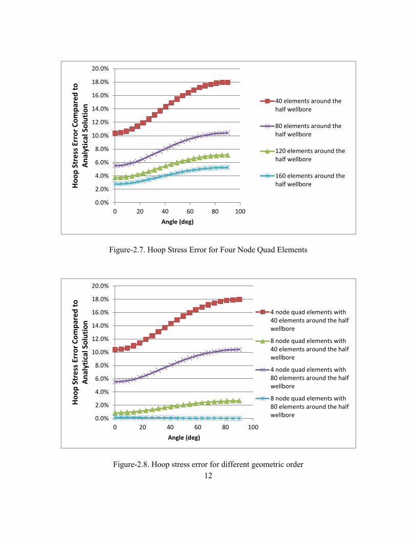
Figure-2.7. Hoop Stress Error for Four Node Quad Elements
Figure-2.8. Hoop stress error for different geometric order
0.0%
2.0%
4.0%
6.0%
8.0%
10.0%
12.0%
14.0%
16.0%
18.0%
20.0%
0 20 40 60 80 100
Ho
op
Str
ess
Erro
r C
om
par
ed t
o
An
alyt
ical
So
luti
on
Angle (deg)
40 elements around thehalf wellbore
80 elements around thehalf wellbore
120 elements around thehalf wellbore
160 elements around thehalf wellbore
0.0%
2.0%
4.0%
6.0%
8.0%
10.0%
12.0%
14.0%
16.0%
18.0%
20.0%
0 20 40 60 80 100
Ho
op
Str
ess
Erro
r C
om
par
ed t
o
An
alyt
ical
So
luti
on
Angle (deg)
4 node quad elements with40 elements around the halfwellbore
8 node quad elements with40 elements around the halfwellbore
4 node quad elements with80 elements around the halfwellbore
8 node quad elements with80 elements around the halfwellbore

13
2.1.3. Fracture Modeling
In stress caging, the pressure required for fracture reopening is considered
essentially to same as the pressure required to propagate a fracture, because it is assumed
that the drilling fluid can seep into the previous fracture even if the near wellbore region
is in compression (Alberty and Mclean, 2004). A fixed-length crack has been defined to
simulate this behavior in a two-dimensional, plane strain, linearly elastic model. To do
this, two quarters of the wellbore are sketched individually and then tied together by
using tie constraint except along the fracture zone. Not using the tie constraint along the
fracture would allow fracture faces to move freely. At the first step, wellbore pressure is
applied to the crack faces as fracture pressure. Figure 2.9 shows forces applied to the
model and the hoop stress distribution while there is a crack present. The dark blue region
is the region with maximum compression, while the red region is the region with
maximum tension.
Figure-2.9. Hoop stress distribution with a fracture
Pw
Pfrac
Pfrac

14
For the second step, a certain number of nodes at the fracture is fixed in terms of
displacement by using velocity boundary condition and a load which is equal to
formation pressure is applied to the fracture faces behind these nodes to simulate
bridging. By doing this, it is assumed that the drilling fluid inside the fracture fully
dissipated into the formation and there will be no increase in local formation pressure. In
addition, the bridge is considered incompressible and it provides an effective seal
between the wellbore pressure and fracture pressure. Location of the bridge and length of
the bridge is variable and can be changed by the user. If there is space between the bridge
and wellbore, wellbore pressure is applied to the fracture faces in front of the bridge. To
simulate closing of the fracture and prevent overlapping of the fracture faces after
bleeding off the pressure inside the fracture, hard contact interaction is defined along the
fracture.
Figure-2.10. Hoop stress distribution with a bridge at the fracture mouth
Pw
Po
Po
15
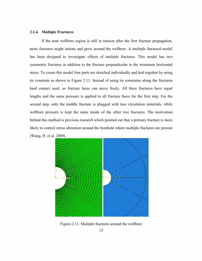
2.1.4. Multiple Fractures
If the near wellbore region is still in tension after the first fracture propagation,
more fractures might initiate and grow around the wellbore. A multiple fractured model
has been designed to investigate effects of multiple fractures. This model has two
symmetric fractures in addition to the fracture perpendicular to the minimum horizontal
stress. To create this model four parts are sketched individually and tied together by using
tie constrain as shown in Figure 2.11. Instead of using tie constrains along the fractures
hard contact used, so fracture faces can move freely. All three fractures have equal
lengths and the same pressure is applied to all fracture faces for the first step. For the
second step, only the middle fracture is plugged with loss circulation materials, while
wellbore pressure is kept the same inside of the other two fractures. The motivation
behind this method is previous research which pointed out that a primary fracture is more
likely to control stress alteration around the borehole where multiple fractures are present
(Wang, H. et al. 2009).
Figure-2.11. Multiple fractures around the wellbore
16
2.2.THREE-DIMENSIONAL MODEL DESCRIPTION
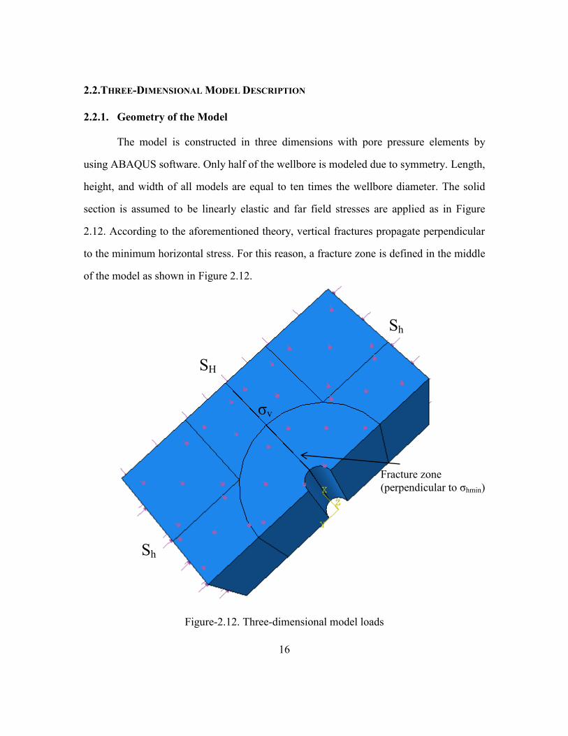
2.2.1. Geometry of the Model
The model is constructed in three dimensions with pore pressure elements by
using ABAQUS software. Only half of the wellbore is modeled due to symmetry. Length,
height, and width of all models are equal to ten times the wellbore diameter. The solid
section is assumed to be linearly elastic and far field stresses are applied as in Figure
2.12. According to the aforementioned theory, vertical fractures propagate perpendicular
to the minimum horizontal stress. For this reason, a fracture zone is defined in the middle
of the model as shown in Figure 2.12.
Figure-2.12. Three-dimensional model loads
SH
Sh
Sh
σv
Fracture zone
(perpendicular to σhmin)

17
2.2.2. Initial and Boundary Conditions
Symmetry boundary condition is applied in the y direction, bottom nodes are
fixed for zero displacement in the z axis, and to make sure nothing moves in the model,
one node in the middle is fixed for zero displacement in the y direction, as shown in
Figure 2.13. Pore pressure, and void ratio is assigned to all nodes as initial conditions.
Void ratio is defined as the ratio of the volume of voids to the volume of solid material.
Single phase flow is assumed and saturation is taken as unity for all simulations.
Permeability is defined in material properties as a function of void ratio and assumed
homogeneous and isotropic.
Figure-2.13. Boundary conditions of the three-dimensional model
Displacement of
this node is zero
in y direction
Displacements of
bottom nodes are
zero in z direction
Symmetry boundary
condition

18
2.2.3. Accuracy of the Model and Mesh
Hoop stress distributions are calculated by the three-dimensional model and
compared with the Kirsch solution for different number of elements around the borehole.
Effective stress components considering pore pressure are given below.
So, the effective stress at the wellbore wall is expressed as;

19
As the complexity of the model increases, element type and mesh become more
important. A structured mesh has been generated with hex shape elements. Denser mesh
improves the accuracy as in two-dimension models but increases the computation time
drastically in three-dimensional analysis. Geometric order of the elements is another
concern. Geometric order of hex shape elements can either be linear with eight nodes or
quadratic with twenty nodes.
Figure-2.14. Hex shape elements with different geometric orders (Abaqus 6.10-EF
Documentation, 2010)
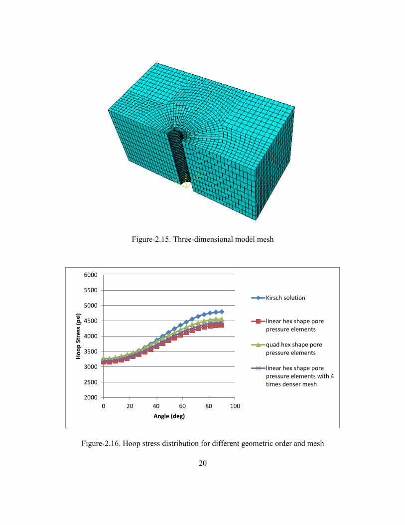
The hoop stress values around the wellbore are calculated for a pre-fractured state
with zero wellbore pressure for different geometric order and mesh. The results are given
in Figure 2.16. Input data used in the model is given in Table 2.
Table-2 Input data for three-dimensional model verification
Wellbore diameter 8.5 inch
Overburden Stress 3000 psi
Max Horizontal Stress 2200 psi
Min Horizontal Stress 1800 psi
Formation Pressure 870 psi
Young Modulus 1740000 psi
Poisson’s ratio 0.25
20
Figure-2.15. Three-dimensional model mesh
Figure-2.16. Hoop stress distribution for different geometric order and mesh
2000
2500
3000
3500
4000
4500
5000
5500
6000
0 20 40 60 80 100
Ho
op
Str
ess
(p
si)
Angle (deg)
Kirsch solution
linear hex shape porepressure elements
quad hex shape porepressure elements
linear hex shape porepressure elements with 4times denser mesh

21
2.2.4. Fracture Modeling
The fracture zone is modeled by using pore-pressure cohesive elements based on
traction-separation modeling. Cracks can only initiate and propagate along this zone and
there is no need of a crack to start with. A crack can initiate in cohesive zone as long as
the initiation criteria are satisfied. Similarly, damage evolution criterion must be satisfied
for fracture propagation.
Figure-2.17. Three-dimensional cohesive element (Abaqus 6.10 Documentation, 2010)
2.2.4.1.Mechanical Behavior of the Fracture Zone
The quadratic nominal stress criterion is used as fracture initiation criteria in the
model. This criterion is satisfied when the following quadratic interaction function
reaches one (Abaqus 6.10-EF Documentation, 2010).
Each term represents the square of nominal stress ratios. Each ratio is the nominal
stress value divided by maximum nominal stress value, where , and are the
maximum values of nominal stress.

22
Fracture propagation criteria are defined by using a damage evolution law. After
initiation criterion is satisfied, the damage evolution law represents the magnitude of
propagation. This magnitude is defined by D which is the overall damage in the material.
The value of D lies between 0 and 1, where D=1 means complete damage. Stress
components affected by the damage are given below (Abaqus 6.10-EF Documentation,
2010).
where, , and are the predicted stress components.
With tensile fractures, Benzeggagh-Kenane fracture criterion given below
describes the problem better than any other criteria, because the critical fracture energies
along the first and second shear directions are equal (Benzeggagh and Kenane, 1996,
Abaqus 6.10-EF Documentation, 2010).
where, GC is the fracture energy dissipated.
In this study all the elastic properties of the fracture zone are taken from a
hydraulically induced fracture problem in Abaqus example problems manual (Abaqus
6.10-EF Documentation, 2010).
23
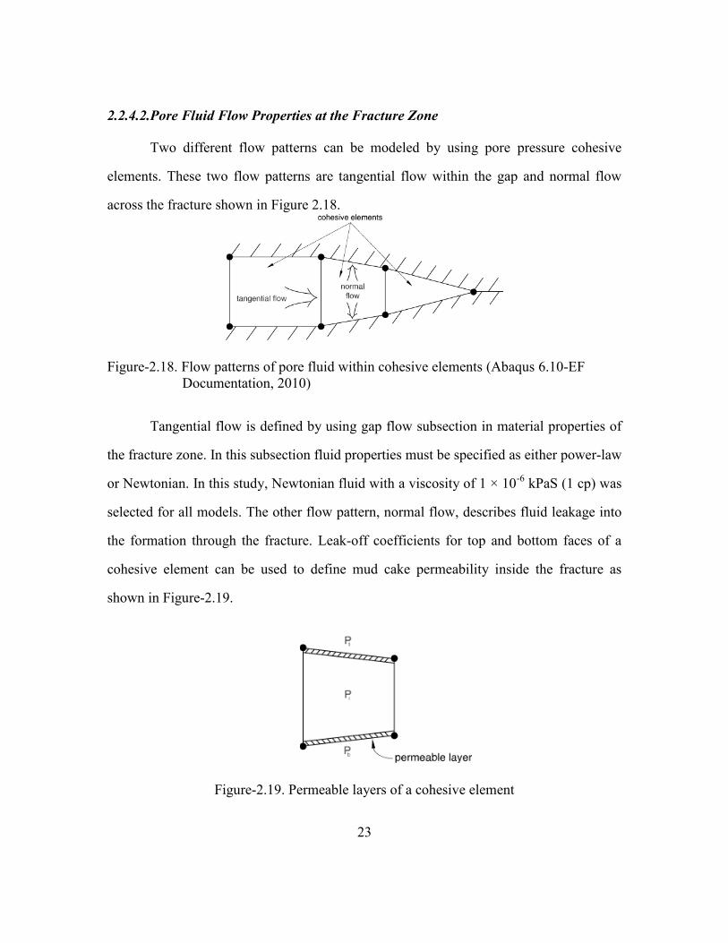
2.2.4.2.Pore Fluid Flow Properties at the Fracture Zone
Two different flow patterns can be modeled by using pore pressure cohesive
elements. These two flow patterns are tangential flow within the gap and normal flow
across the fracture shown in Figure 2.18.
Figure-2.18. Flow patterns of pore fluid within cohesive elements (Abaqus 6.10-EF
Documentation, 2010)
Tangential flow is defined by using gap flow subsection in material properties of
the fracture zone. In this subsection fluid properties must be specified as either power-law
or Newtonian. In this study, Newtonian fluid with a viscosity of 1 × 10⁻⁶
kPaS (1 cp) was
selected for all models. The other flow pattern, normal flow, describes fluid leakage into
the formation through the fracture. Leak-off coefficients for top and bottom faces of a
cohesive element can be used to define mud cake permeability inside the fracture as
shown in Figure-2.19.
Figure-2.19. Permeable layers of a cohesive element

24
In the modeled case, it is assumed that leak-off coefficients are equal for both
faces and normal flow is defined as;
( )
where, c is the leak-off coefficient and q is the flow rate into the formation.
Unfortunately, no experimental data have been reported in terms of leak-off
coefficient. Leak-off coefficient values used in this model are also taken from
hydraulically induced fracture problem in ABAQUS example problems manual.

25
3. Results
3.1.TWO-DIMENSIONAL ANALYSIS OF WELLBORE STRENGTHENING
First run of the two-dimensional model for an example application of wellbore
strengthening consists of three steps. First step gives the stress distribution around the
wellbore to identify fracture initiation pressure. In the second step, a fixed length crack
has been added to the model and the initiation pressure found at the first step is applied to
the wellbore and fracture faces. Fracture mouth is fixed by using velocity boundary
condition to simulate plugging at the last step. Input data used in the simulation is given
in Table 3.
Table-3 Input data for two-dimensional analysis
Wellbore diameter 8.5 inch 0.10795 m
Model Dimensions 85x85x85 inch 1.0795x1.0795x1.0795 m
Max Horizontal Stress 2200 psi 15150 kPa
Min Horizontal Stress 1800 psi 12400 kPa
Formation Pressure 870 psi 6000 kPa
Young Modulus 1740000 psi 1.2e7 kPa
Poisson’s ratio 0.25 0.25
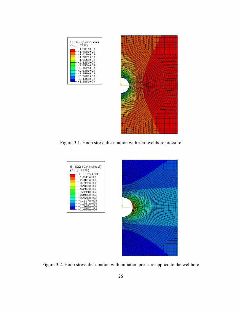
Second order quad shape elements are used for all two-dimensional analysis to
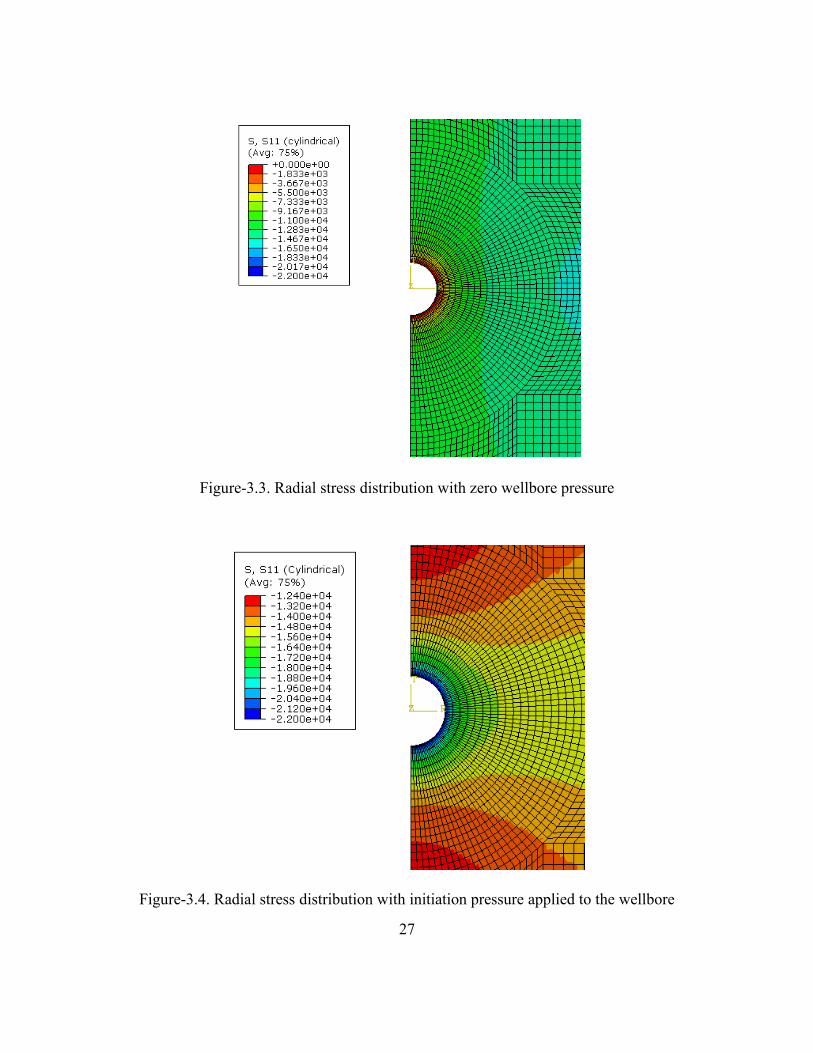
yield the most accurate results. For comparison, hoop stress and radial stress distributions
are given in Figure 3.1-3.4. These figures are taken from ABAQUS software. Negative
sign in ABAQUS corresponds to compression, while positive sign corresponds to
tension. Also, units in ABAQUS legend are kPA. ABAQUS stress values multiplied by
“–1” and units converted to field units in Excel graphs. No wellbore pressure is applied
in Figure 3.1 and 3.3. Hoop stress value at zero degree, from Figure 3.1 is used as the
fracture initiation pressure in the next step.
26
Figure-3.1. Hoop stress distribution with zero wellbore pressure
Figure-3.2. Hoop stress distribution with initiation pressure applied to the wellbore
27
Figure-3.3. Radial stress distribution with zero wellbore pressure
Figure-3.4. Radial stress distribution with initiation pressure applied to the wellbore
28
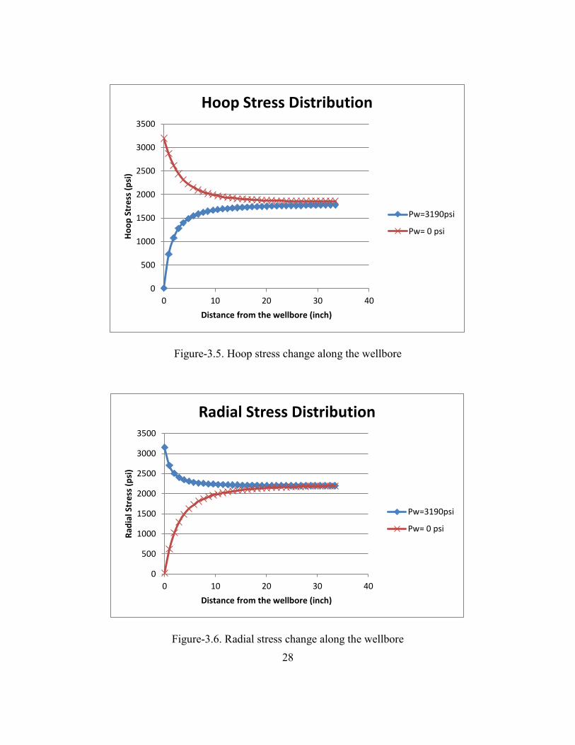
Figure-3.5. Hoop stress change along the wellbore
Figure-3.6. Radial stress change along the wellbore
0
500
1000
1500
2000
2500
3000
3500
0 10 20 30 40
Ho
op
Str
ess
(p
si)
Distance from the wellbore (inch)
Hoop Stress Distribution
Pw=3190psi
Pw= 0 psi
0
500
1000
1500
2000
2500
3000
3500
0 10 20 30 40
Rad
ial S
tre
ss (
psi
)
Distance from the wellbore (inch)
Radial Stress Distribution
Pw=3190psi
Pw= 0 psi

29
Figure-3.7. Hoop stress distribution after fracture propagation (deformations magnified
20 times)
During the second step, a fixed length fracture propagates instantly. Figure 3.7
shows the hoop distribution with a propagated fracture. Compression around the wellbore
increases as the fracture gains width. The increase in compression is much higher in the
region close to the fracture as shown in Figure 3.7. The fracture tip is the region with
high tension. If this tension is higher than rock can withstand, fracture growth is
expected. In this case, fracture is not growing regardless of high tension because the
fracture length is fixed in the two-dimension model. The third step simulates wellbore
strengthening by plugging the fracture with loss circulation materials. For this case, the
location of the bridge is the first element at the fracture mouth. Also, length of the bridge
equals to the length of this element. The particle diameter is assumed to be the same size
as the fracture width and it is not moving or losing volume inside the fracture. After
30
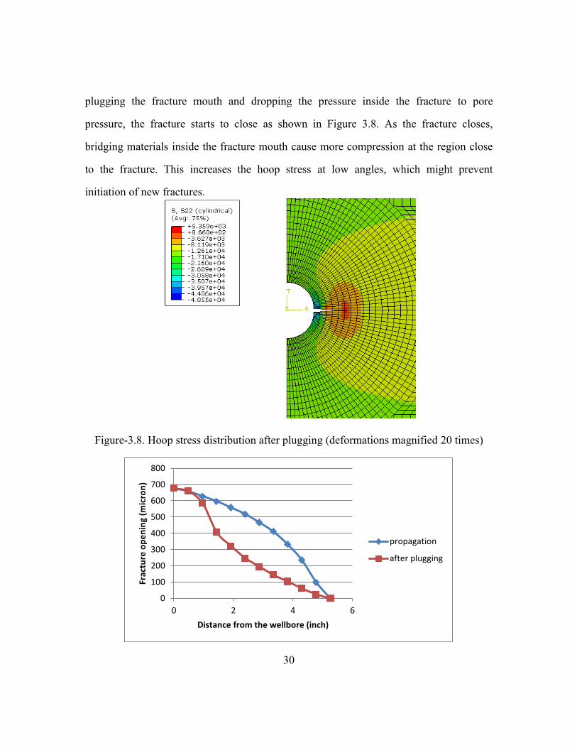
plugging the fracture mouth and dropping the pressure inside the fracture to pore
pressure, the fracture starts to close as shown in Figure 3.8. As the fracture closes,
bridging materials inside the fracture mouth cause more compression at the region close
to the fracture. This increases the hoop stress at low angles, which might prevent
initiation of new fractures.
Figure-3.8. Hoop stress distribution after plugging (deformations magnified 20 times)
0
100
200
300
400
500
600
700
800
0 2 4 6
Frac
ture
op
en
ing
(mic
ron
)
Distance from the wellbore (inch)
propagation
after plugging
31
Figure-3.9. Change in fracture opening after plugging
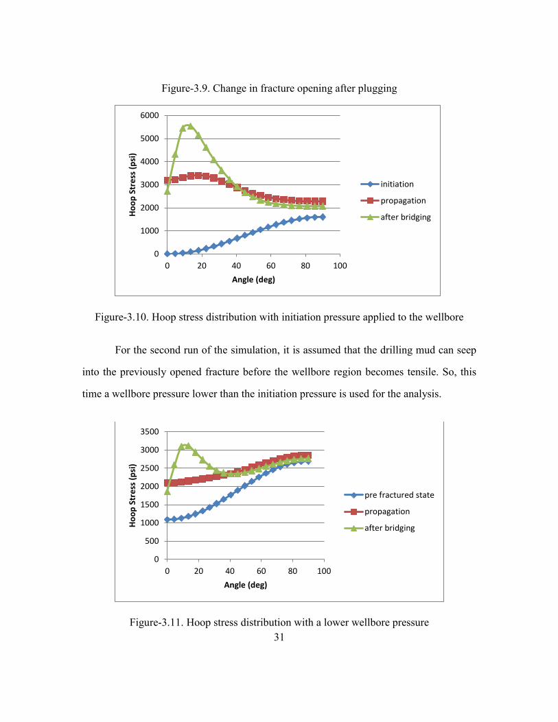
Figure-3.10. Hoop stress distribution with initiation pressure applied to the wellbore
For the second run of the simulation, it is assumed that the drilling mud can seep
into the previously opened fracture before the wellbore region becomes tensile. So, this
time a wellbore pressure lower than the initiation pressure is used for the analysis.
Figure-3.11. Hoop stress distribution with a lower wellbore pressure
0
1000
2000
3000
4000
5000
6000
0 20 40 60 80 100
Ho
op
Str
ess
(p
si)
Angle (deg)
initiation
propagation
after bridging
0
500
1000
1500
2000
2500
3000
3500
0 20 40 60 80 100
Ho
op
Str
ess
(p
si)
Angle (deg)
pre fractured state
propagation
after bridging

32
Figures 3.10 and 3.11 have similar trend, the difference in the compressive trend
after fracture propagation is due to the change in fracture width. As the pressure applied
to the fracture faces increase, fracture width increases.
Figure-3.12. Fracture opening for different wellbore pressures
However wellbore pressure is not the only factor affecting the fracture width.
Stress anisotropy can also change the fracture width. For this reason, another simulation
is designed to investigate effects of stress anisotropy. Three different horizontal stress
ratios are used in the simulations by changing minimum horizontal stress. All data
besides minimum horizontal stress are taken constant. Fracture openings for different
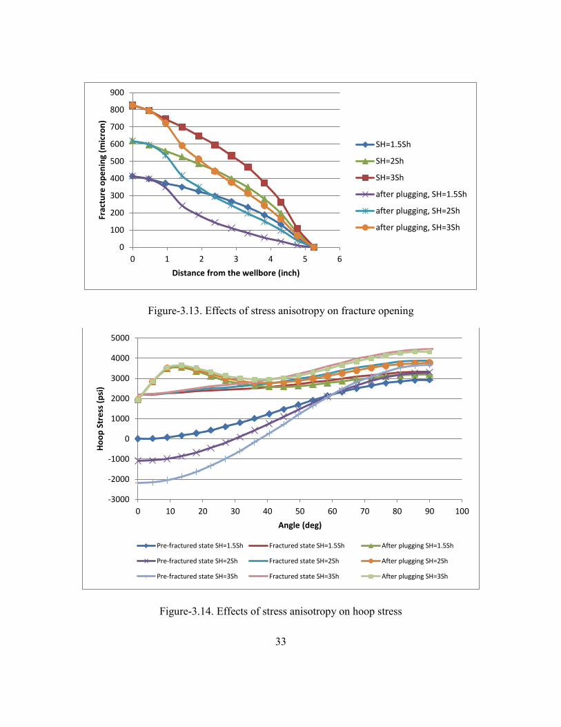
stress ratios are given in Figure 3.13. It can be seen that fracture width is directly
proportional to the degree of anisotropy. Hoop stress values calculated for pre-fractured
state, with a fracture present and after plugging show similar trends in Figure 3.14. Even
though the fracture width increases, lower horizontal stress is results in lower
compression. Therefore, they compensate each other and generate the trend in Figure
3.14.
0
100
200
300
400
500
600
700
800
0 1 2 3 4 5 6
Frac
ture
op
en
ing
(mic
ron
)
Distance from the wellbore (inch)
Pw=3190 psi
Pw=2650 psi
Pw=2100 psi
33
Figure-3.13. Effects of stress anisotropy on fracture opening
Figure-3.14. Effects of stress anisotropy on hoop stress
0
100
200
300
400
500
600
700
800
900
0 1 2 3 4 5 6
Frac
ture
op
en
ing
(mic
ron
)
Distance from the wellbore (inch)
SH=1.5Sh
SH=2Sh
SH=3Sh
after plugging, SH=1.5Sh
after plugging, SH=2Sh
after plugging, SH=3Sh
-3000
-2000
-1000
0
1000
2000
3000
4000
5000
0 10 20 30 40 50 60 70 80 90 100
Ho
op
Str
ess
(p
si)
Angle (deg)
Pre-fractured state SH=1.5Sh Fractured state SH=1.5Sh After plugging SH=1.5Sh
Pre-fractured state SH=2Sh Fractured state SH=2Sh After plugging SH=2Sh
Pre-fractured state SH=3Sh Fractured state SH=3Sh After plugging SH=3Sh
34
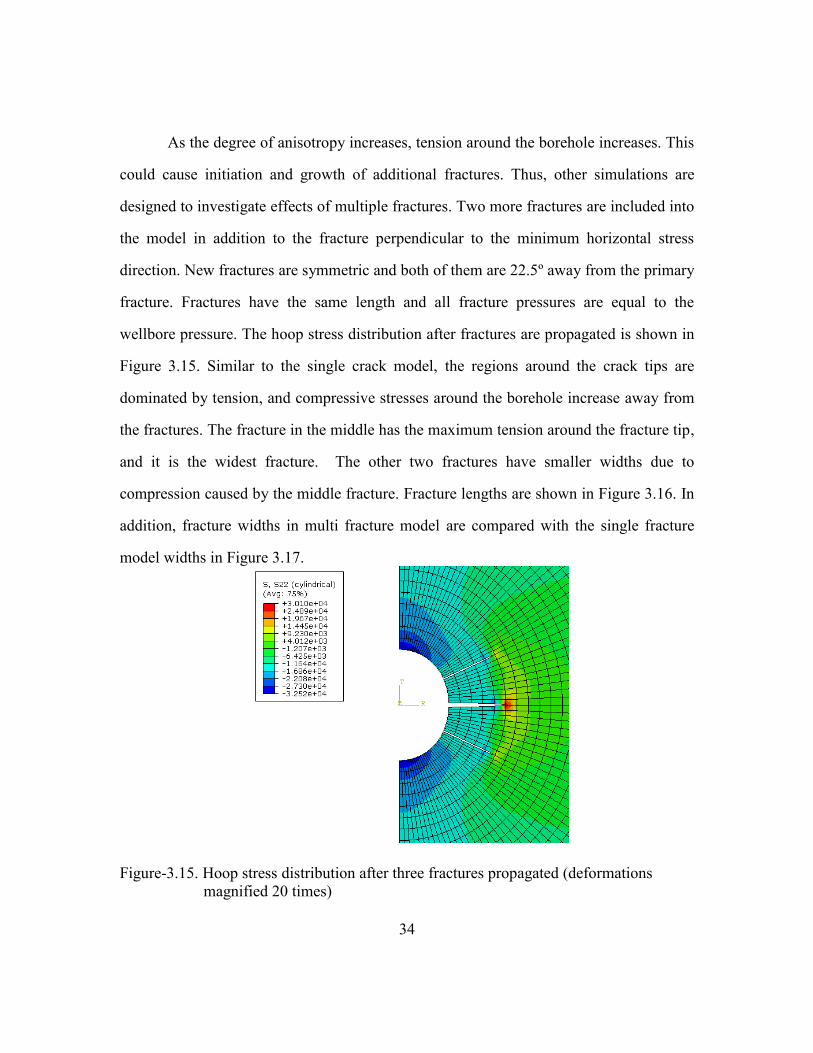
As the degree of anisotropy increases, tension around the borehole increases. This
could cause initiation and growth of additional fractures. Thus, other simulations are
designed to investigate effects of multiple fractures. Two more fractures are included into
the model in addition to the fracture perpendicular to the minimum horizontal stress
direction. New fractures are symmetric and both of them are 22.5º away from the primary
fracture. Fractures have the same length and all fracture pressures are equal to the
wellbore pressure. The hoop stress distribution after fractures are propagated is shown in
Figure 3.15. Similar to the single crack model, the regions around the crack tips are
dominated by tension, and compressive stresses around the borehole increase away from
the fractures. The fracture in the middle has the maximum tension around the fracture tip,
and it is the widest fracture. The other two fractures have smaller widths due to
compression caused by the middle fracture. Fracture lengths are shown in Figure 3.16. In
addition, fracture widths in multi fracture model are compared with the single fracture
model widths in Figure 3.17.
Figure-3.15. Hoop stress distribution after three fractures propagated (deformations
magnified 20 times)

35
Figure-3.16. Fracture lengths in multi fracture model
Figure-3.17. Fracture width comparison between single and multi fracture models
0
100
200
300
400
500
600
0 1 2 3 4 5 6
Frac
ture
Wid
th (
mic
ron
)
Fracture Length (inch)
primary fracture(SH=3Sh)
secondary fracture(SH=3Sh)
primary fracture(SH=2Sh)
secondary fracture(SH=2Sh)
primary fracture(SH=1.5Sh)
secondary fracture(SH=1.5Sh)
0
100
200
300
400
500
600
700
800
900
0 1 2 3 4 5 6
Frac
ture
Wid
th (
mic
ron
)
Fracture Length (inch)
single fracture model(SH=3Sh)
single fracture model(SH=2Sh)
single fracture model(SH=1.5Sh)
multi fracture model(SH=3Sh)
multi fracture model(SH=2Sh)
multi fracturemodel(SH=1.5Sh)
36
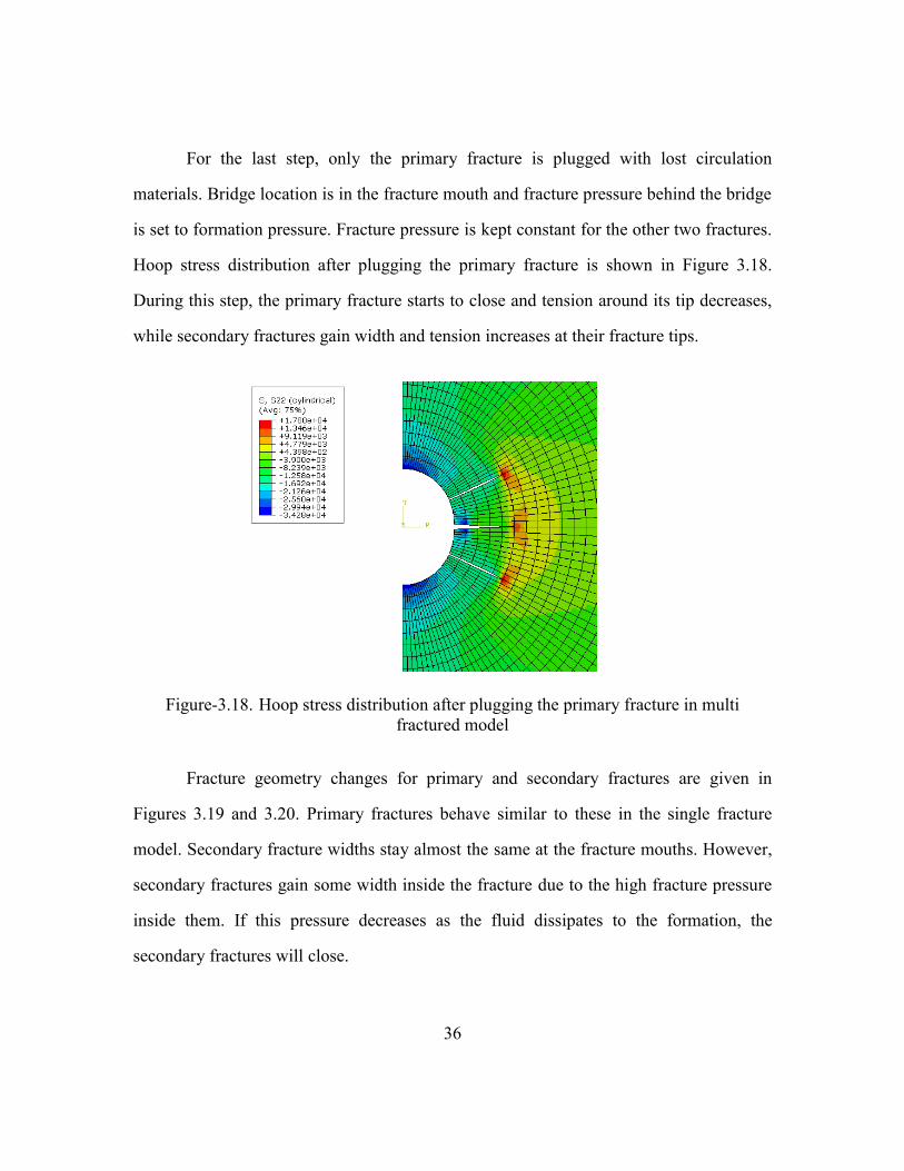
For the last step, only the primary fracture is plugged with lost circulation
materials. Bridge location is in the fracture mouth and fracture pressure behind the bridge
is set to formation pressure. Fracture pressure is kept constant for the other two fractures.
Hoop stress distribution after plugging the primary fracture is shown in Figure 3.18.
During this step, the primary fracture starts to close and tension around its tip decreases,
while secondary fractures gain width and tension increases at their fracture tips.
Figure-3.18. Hoop stress distribution after plugging the primary fracture in multi
fractured model
Fracture geometry changes for primary and secondary fractures are given in
Figures 3.19 and 3.20. Primary fractures behave similar to these in the single fracture
model. Secondary fracture widths stay almost the same at the fracture mouths. However,
secondary fractures gain some width inside the fracture due to the high fracture pressure
inside them. If this pressure decreases as the fluid dissipates to the formation, the
secondary fractures will close.

37
Figure-3.19. Change in primary fracture opening in multi fracture model
Figure-3.20. Change in secondary fracture opening in multi fracture model
0
100
200
300
400
500
600
0 1 2 3 4 5 6
Frac
ture
Wid
th (
mic
ron
)
Fracture Length (inch)
primary fracture (SH=3Sh)
primary fracture afterplugging (SH=3Sh)
primary fracture (SH=2Sh)
primary fracture afterplugging (SH=2Sh)
primary fracture (SH=1.5Sh)
primary fracture afterplugging (SH=1.5Sh)
0
50
100
150
200
250
0 2 4 6
Frac
ture
Wid
th (
mic
ron
)
Fracture Length (inch)
secondary fracture (SH=1.5Sh)
secondary fracture after pluggingthe middle fracture (SH=1.5Sh)
secondary fracture (SH=3Sh)
secondary fracture after pluggingthe middle fracture (SH=3Sh)
secondary fracture (SH=2Sh)
secondary fracture after pluggingthe middle fracture (SH=2Sh)
38
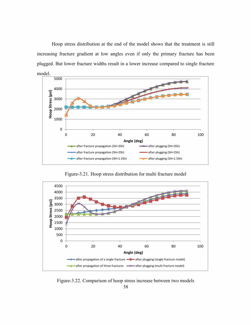
Hoop stress distribution at the end of the model shows that the treatment is still
increasing fracture gradient at low angles even if only the primary fracture has been
plugged. But lower fracture widths result in a lower increase compared to single fracture
model.
Figure-3.21. Hoop stress distribution for multi fracture model
Figure-3.22. Comparison of hoop stress increase between two models
0
1000
2000
3000
4000
5000
0 20 40 60 80 100
Ho
op
Str
ess
(p
si)
Angle (deg) after fracture propagation (SH=3Sh) after plugging (SH=3Sh)
after fracture propagation (SH=2Sh) after plugging (SH=2Sh)
after fracture propagation (SH=1.5Sh) after plugging (SH=1.5Sh)
0
500
1000
1500
2000
2500
3000
3500
4000
4500
0 20 40 60 80 100
Ho
op
Str
ess
(p
si)
Angle (deg)
after propagation of a single fracture after plugging (single fracture model)
after propagation of three fractures after plugging (multi fracture model)
39
3.2.THREE-DIMENSIONAL ANALYSIS OF WELLBORE STRENGTHENING
To investigate factors effecting wellbore strengthening more precisely, results
from a three-dimensional model with pore pressure needs to be studied carefully. A tree-
dimensional model for this study consists of three steps. Fracture initiation pressure is
applied to the wellbore for the first step to create tension at the fracture zone. After
initiation criterion is satisfied, fluid flow into the fracture is defined and fracture
propagation is observed in the second step. In the third and final step, the fracture is
plugged with lost circulation materials. These materials create an effective sealing
between wellbore pressure and fracture tip. At the end of the third step, pressure inside
the fracture is dissipated to the formation. Input data used in the following simulations
are given in Table 4.
Table-4 Input data for three-dimensional analysis
Wellbore diameter 8.5 inch 0.10795 m
Model Dimensions 85x85x85 inch 1.0795x1.0795x1.0795 m
Overburden Stress 3000 psi 20700 kPa
Max Horizontal Stress 2200 psi 15150 kPa
Min Horizontal Stress 1465 psi 10100 kPa
Formation Pressure 870 psi 6000 kPa
Porosity 0.32 0.32
Permeability 160 md 16x10-14m2
viscosity 1cp 1x10⁻⁶ kPas
Young Modulus 1740000 psi 1.2e7 kPa
Poisson’s ratio 0.25 0.25
Flow rate into the fracture 0.015 bbl/min 4x10⁻⁵ m3/s
40
Figure-3.23. Hoop stress distribution at the end of first step in three-dimensional model
Figure-3.24. Hoop stress distribution after fracture propagation in three-dimensional
model (deformation magnified 50 times)
41
Figure-3.25. Hoop stress distribution after plugging the fracture in three-dimensional
model (deformation magnified 50 times)
Figure-3.26. Fracture geometry in three-dimensional model
0
50
100
150
200
250
300
350
400
450
0 10 20 30 40 50
Frac
ture
Wid
th (
mic
ron
)
Fracture Length (inch)
after fracture propagation
after plugging
42
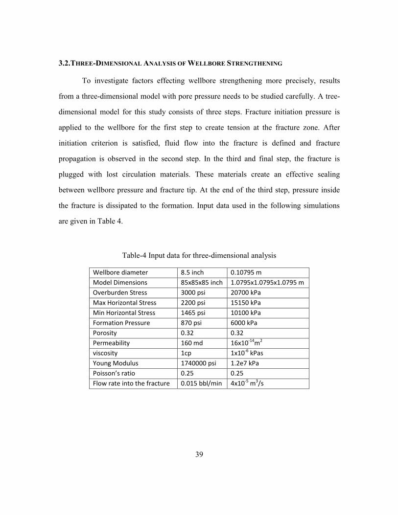
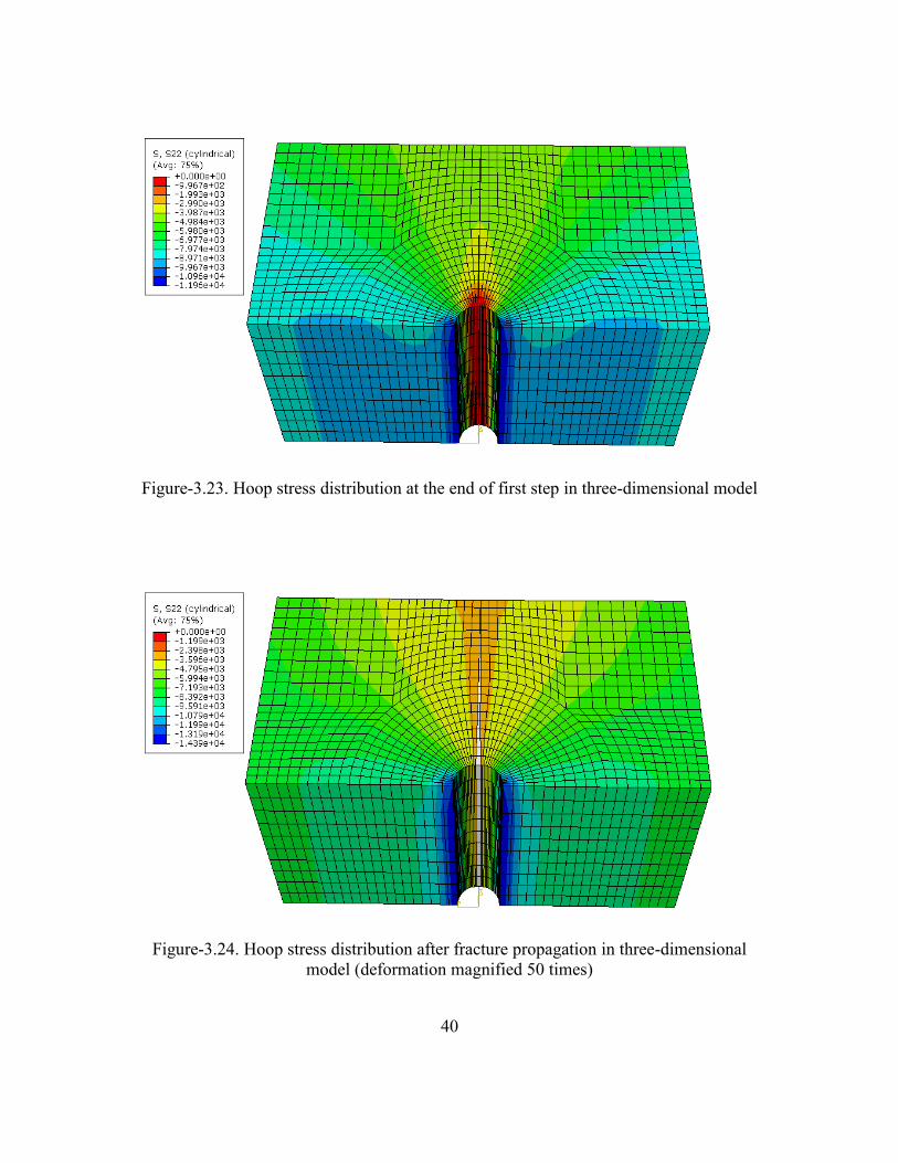
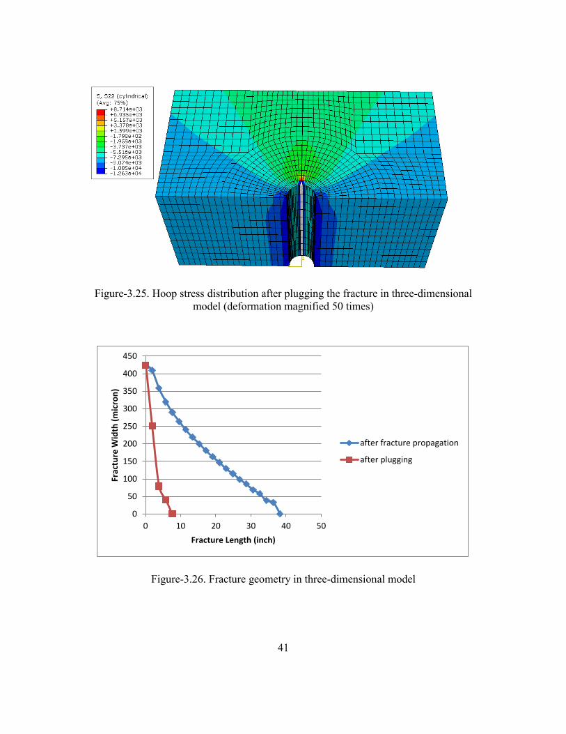
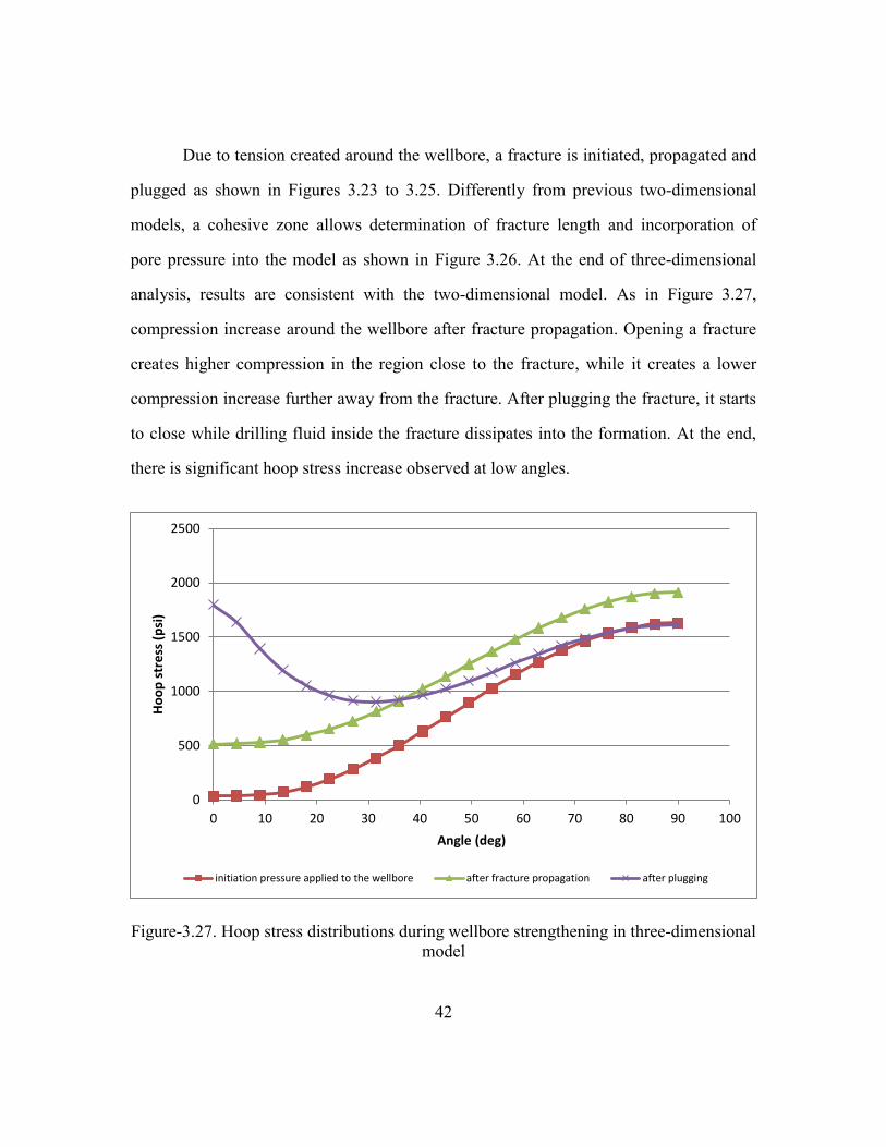
Due to tension created around the wellbore, a fracture is initiated, propagated and
plugged as shown in Figures 3.23 to 3.25. Differently from previous two-dimensional
models, a cohesive zone allows determination of fracture length and incorporation of
pore pressure into the model as shown in Figure 3.26. At the end of three-dimensional
analysis, results are consistent with the two-dimensional model. As in Figure 3.27,
compression increase around the wellbore after fracture propagation. Opening a fracture
creates higher compression in the region close to the fracture, while it creates a lower
compression increase further away from the fracture. After plugging the fracture, it starts
to close while drilling fluid inside the fracture dissipates into the formation. At the end,
there is significant hoop stress increase observed at low angles.
Figure-3.27. Hoop stress distributions during wellbore strengthening in three-dimensional
model
0
500
1000
1500
2000
2500
0 10 20 30 40 50 60 70 80 90 100
Ho
op
str
ess
(p
si)
Angle (deg)
initiation pressure applied to the wellbore after fracture propagation after plugging

43
As mentioned before, rate of fluid loss must be defined in the model to determine
fracture geometry. Figure 3.28 shows fracture geometry for different fluid losses.
Fluctuation in the figure is because of model length. Some fractures are actually longer
than the model but boundary conditions restricted into growth. In this case, a trend-line
can be added to determine actual fracture length instead of using a longer model.
Figure-3.28. Fracture geometry for different loss rates
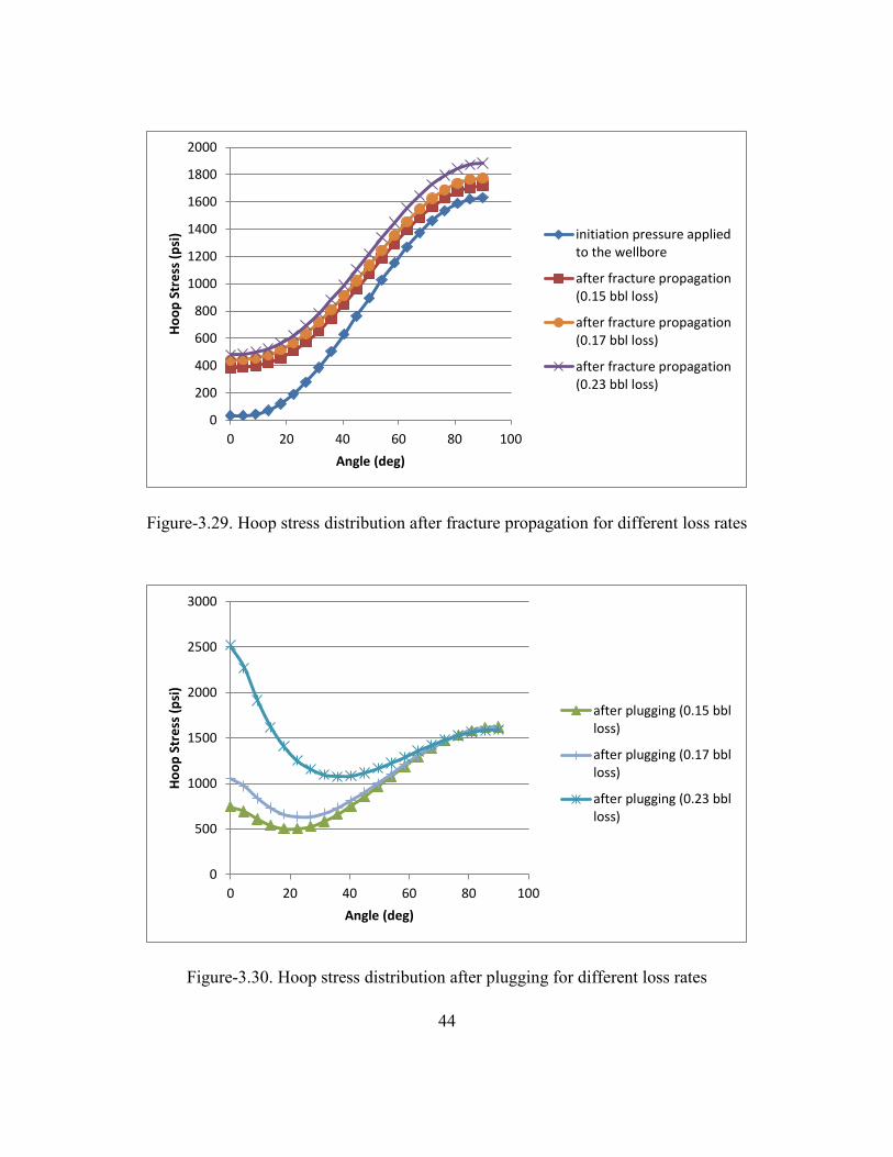
Compression created around the wellbore due to a fracture is directly related with
the fracture width. Wider fractures cause higher compression around the wellbore as
shown in Figure 3.29. Moreover, plugging a wider fracture creates a higher hoop stress
increase during wellbore strengthening as shown in Figure 3.30.
0
100
200
300
400
500
600
0 10 20 30 40 50
Frac
ture
Wid
th (
mic
ron
)
Fracture Length (inch)
after fracturepropagation (0.23bbl loss)
after fracturepropagation (0.17bbl loss)
after fracturepropagation (0.15bbl loss)
44
Figure-3.29. Hoop stress distribution after fracture propagation for different loss rates
Figure-3.30. Hoop stress distribution after plugging for different loss rates
0
200
400
600
800
1000
1200
1400
1600
1800
2000
0 20 40 60 80 100
Ho
op
Str
ess
(p
si)
Angle (deg)
initiation pressure appliedto the wellbore
after fracture propagation(0.15 bbl loss)
after fracture propagation(0.17 bbl loss)
after fracture propagation(0.23 bbl loss)
0
500
1000
1500
2000
2500
3000
0 20 40 60 80 100
Ho
op
Str
ess
(p
si)
Angle (deg)
after plugging (0.15 bblloss)
after plugging (0.17 bblloss)
after plugging (0.23 bblloss)

45
Effects of permeability can be observed in this finite element model. During
propagation of a fracture, more fluid flows into the formation in highly permeable rocks.
This will reduce the fracture pressure and decreases fracture growth. Decrease in fracture
growth then decreases compression around the wellbore.
Figure-3.31. Effects of permeability on fracture growth
Figure-3.32. Effects of permeability on hoop stress
-10
0
10
20
30
40
50
60
70
0 10 20 30 40 50
Frac
ture
Wid
th (
mic
ron
)
Fracture Length (inch)
160 md
80 md
0
500
1000
1500
2000
0 20 40 60 80 100
Ho
op
str
ess
(p
si)
Angle (deg)
initiation pressure applied to the wellbore (160 md) after fracture propagation (160 md)
after plugging (160 md) initiation pressure applied to the wellbore (80 md)
after fracture propagation (80 md) after plugging (80 md)

46
Another important factor is mud cake permeability inside the fracture. The
aforementioned leak-off option is used to simulate this behavior by defining a leak-off
coefficient. A low leak-off coefficient corresponds to low mud cake permeability.
Similarly, as rock permeability, more fluid flow into the formation reduces fracture
pressure and growth.
Figure-3.33. Effects of mud cake permeability on fracture growth
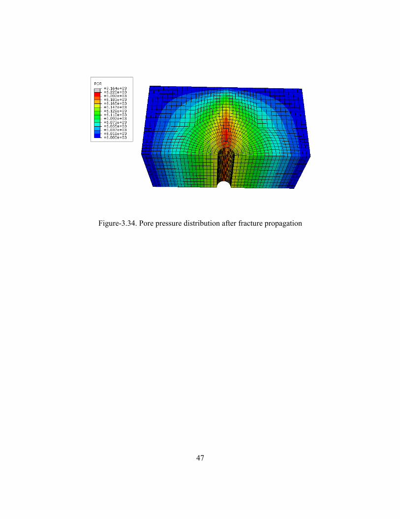
Furthermore, the leak-off coefficient is a very important factor that determines pore
pressure distribution around the wellbore during fracture propagation as well as the rate
of fluid loss. However, there are no correlations between this value and lab experiments
yet (Salehi and Nygaard, 2010). In the simulation in this thesis, the leak-off coefficient is
an arbitrary number. The pore pressure distributions using this value are shown in figure
3.34. The highest values correspond to color grey is the pressure inside the fracture.
-20
0
20
40
60
80
100
120
140
160
0 10 20 30 40 50
Frac
ture
Wid
th (
mic
ron
)
Fracture Length (inch)
high mud cakepermeability
low mud cakepermeability
47
Figure-3.34. Pore pressure distribution after fracture propagation
48
4. Conclusions
The objective of this thesis was to develop detailed finite element models and
procedures to investigate factors effecting wellbore strengthening. ABAQUS software
was used to develop finite element models. Development started with a two-dimensional,
plane strain, linearly elastic model and upgraded to a three-dimensional model with
consideration of pore pressure effects. The models developed can simulate initiation and
propagation of a fracture. Furthermore, the models can quantify stress distributions
around the wellbore after plugging the fracture with loss circulation materials. Moreover,
fracture geometry length and width can be observed in three-dimensional model. The
following conclusions can be drawn from the simulation results;
Opening a fracture increases compression around the wellbore. This
increase is highest in regions close to the fracture compared to regions
further away.
Plugging the fracture mouth with loss circulation materials does not
increase the hoop stress everywhere around the wellbore. It increases the
hoop stress at the near wellbore region close to the fracture and it may
prevent opening and growth of additional fractures.
Fracture width is the most significant factor to increase hoop stress, if the
bridging material can keep the fracture open and sealed.
After plugging the fracture mouth, the weakest point around the wellbore
changes. Because of this, if the wellbore pressure is increased to new
initiation pressures after treatment, new fractures grow in new directions.
If there is more than one fracture present, fractures will be smaller than
expected and their size differs based on fracture location.
49
As the formation permeability or mud cake permeability increases,
fracture length and width decreases, because more fluid will flow into the
formation. Thus, pressure felt by the fracture tip decreases.
Finally, for future work, finite element models should be tested with detailed field
data and confirmed by using field results of wellbore strengthening applications.
Moreover, additional experimental studies are required to calibrate the models.

50
References
ABAQUS/CAE 6.10 EF, Analysis User’s Manual, 2010.
Aadnoy, B.S.; Belayneh, M. “A New Fracture Model That Includes Load History,
Temperature, and Poisson’s Effects”, SPE Drilling & Completion, 452-455,
September, 2009.
Alberty, M.W. and Mclean, M. R. “A Physical Model for Stress Cages”, SPE 90493, SPE
Annual Technical Conference, Houston, September 26-29, 2004.
Aston, M. S., Alberty, M.W., Mclean, M. R., de Jong, H.J. and Armagost, K. “Drilling
Fluids for Wellbore Strengthening”, SPE 87130, SPE/IADC Drilling Conference,
Dallas, March 2-4,2004.
Aston, M.S. et al. “A New Treatment for Wellbore Strengthening in Shale”, SPE 110713,
SPE Annual Technical Conference and Exhibition, Anaheim California, USA,
November 11-14, 2007.
Benzeggagh, M.L. and Kenane, M. “Measurement of Mixed-Mode Delamination
Fracture Toughness of Unidirectional Glass/Epoxy Composites with Mixed-Mode
Bending Apparatus,” Composite Science and Technology, vol. 56, p. 439, 1996.
Dupriest, F.E. “Fracture Closure Stress (FCS) and Lost Returns Practices” SPE 92192,
SPE/IADC Drilling Conference, Amsterdam, February 23-25, 2005.
Dupriest, F.E., Smith, M.V. and Zeilinger, S. “Method to Eliminate Lost Returns and
Build Integrity Continuously with High-Filtration-Rate Fluid.” SPE 112656,
SPE/IADC Drilling Conference, Orlando, Florida, 4-6 March 2008.
Fuh, G-F., Morita, N. Boyd, P.A. and McGoffin, S.J. “A New Approach to Preventing
Lost Circulation while Drilling,” SPE 24599, 67th
Annual Technical Conference
and Exhibition, Washington D.C., October 4-7, 1992.
Grayson, B., 2009 “Increased Operational Safety and Efficiency with Managed Pressure
Drilling”, IADC/SPE 120982, SPE Americas E&P Environmental Safety
Conference, San Antonio, Texas, USA, 23-25 March 2009.

51
Hubbert, M. K. and Willis, D. G., “Mechanics of Hydraulic Fracturing”, Trans. AIME,
Vol 210, pp-153-166, 1957.
Messenger, J. U.: Lost Circulation, PennWell Publishing Company, Tulsa, Oklahoma,
1981.
Morita, N., Black, A. D., and Fuh, G. F., "Theory of Lost Circulation Pressure," SPE
20409, 65th Annual Technical Conference and Exhibition of the Society of
Petroleum Engineers, pp. 43-58, 1990.
Peng, S., Zhang, J. “Engineering Geology for Underground Rocks”, Springer, July, 2007.
Salehi, S., Nygaard, R., “Finite-element analysis of deliberately increasing the wellbore
fracture gradient”, ARMA 10-202, 44th
US Rock Mechanics Symposium and 5th
U.S.-Canada Rock Mechanics Symposium, Salt Lake City, UT June 27-30, 2010.
Salehi, S., Nygaard, R., “Evaluation of New Drilling Approach for Widening Operational
Window: Implications for Wellbore Strengthening”, SPE 140753, SPE Production
and Operations Symposium, Oklahoma City, Oklahoma, USA, March 27-29,
2011.
Van Oort, E. Friedheim, J., Pierce, T., Lee, J., “Avoiding Losses in Depleted and Weak
Zones by Constantly Strengthening Wellbores”, SPE 125093, SPE Annual
Technical Conference and Exhibition, New Orleans, Louisiana, USA, October
4-7, 2009.
Wang, H. et al. “Fractured Wellbore Stress Analysis- Can Sealing Micro-Cracks Really
Strengthen a Wellbore?”, SPE/IADC 104947, SPE/AIDC Drilling Conference,
Amsterdam, February 20-22, 2007.
Wang, H, Tower, B.F. and Mohamed, S.Y. “Near Wellbore Stress Analysis and Wellbore
Strengthening for Drilling Depleted Formations”, SPE 102719, SPE Rocky
Mountain Oil & Gas Technology Symposium, Denver, Colorado, USA, April
16-18, 2007.
52
Wang, H., et al. “Investigation of Factors for Strengthening a Wellbore by Propping
Fractures”, SPE/IADC 112629, IADC/SPE Drilling Conference, Orlando, Florida,
March 4-6, 2008.
Wang, H., Soliman, M.Y., Towler, B.F., Shan, Z., “Strengthening a Wellbore with
Multiple Fractures: Further Investigation of Factors for Strengthening a
Wellbore”, ARMA 09-67, 43rd
US Rock Mechanics Symposium and 4th
U.S.-
Canada Rock Mechanics Symposium, Asheville, NC June 28th
- July 1, 2009.