contents n - university of california, berkeley · pdf filecontents 3. nonlinear ... kkt...

Preliminarydraftonly:pleasecheckforfinalversion

ARE211, Fall2015

NPP1: THU, SEP 17, 2015 PRINTED: AUGUST 25, 2015 (LEC# 7)

Contents

3. Nonlinear Programming Problems and the Karush Kuhn Tucker conditions 2

3.1. KKT conditions and the Lagrangian: a “cook-book” example 4

3.1. Separating Hyperplanes 7

3.2. Convex sets, quasi- functions and constrained optimization 8

3.3. The setup 10

3.4. Existence and Uniqueness 11

3.5. Necessary conditions for a solution to an NPP 13

3.6. KKT conditions and the Lagrangian approach 15

3.7. Role of the Constraint Qualification 17

3.8. Binding constraints vs constraints satisfied with equality 20

3.9. Interpretation of the Lagrange Multiplier 22

3.10. Demonstration that KKT conditions are necessary 24

3.11. KKT conditions with equality constraints 29

1

2 NPP1: THU, SEP 17, 2015 PRINTED: AUGUST 25, 2015 (LEC# 7)

3. Nonlinear Programming Problems and the Karush Kuhn Tucker conditions

Key points:

(1) The issues

(a) convex sets, quasi- functions and constrained optimization

(b) conditions for existence of a unique solution

(c) necessary conditions for x to be a unique solution

(d) sufficient conditions for x to be a unique solution

(2) The canonical form of the nonlinear programming problem (NPP)

maximize f(x) subject to g(x) ≤ b,

(3) Conditions for existence of a solution the NPP:

Theorem: If f : A → R is continuous and strictly quasi-concave, and A is compact, nonempty

and convex, then f attains a unique maximum on A.

(4) Necessity Conditions relating a local maximum on the constraint set to a unique solution

to the NPP:

Theorem: If f : Rn → R is continuous and strictly quasi-concave and gj : Rn → R is quasi-

convex for each j, then if f attains a local maximum on A = {x ∈ Rn : ∀j, gj(x) ≤ bj}, this

max is the unique global maximum of f on A.

(5) The KKT conditions in Mantra format:

(Except for a bizarre exception) a necessary condition for x to solve a constrained maxi-

mization problem is that the gradient vector of the objective function at x belongs to the

nonnegative cone defined by the gradient vectors of the constraints that are satisfied with

equality at x.

(6) The KKT conditions in math format:

If x solves the maximization problem and the constraint qualification holds at x then there

exists a vector λλλ ∈ Rm+ such that

▽f(x)T = λλλTJg(x)

Moreover, λλλ has the property that λj = 0, for each j such that gj(x) < bj.

ARE211, Fall2015 3

(7) The distinction between a constraint satisfied with equality and a binding constraint.

(8) The role of the constraint qualification (CQ):

(a) it ensures that the linearized version of the constraint set is, locally, a good approxi-

mation of the true nonlinear constraint set.

(b) the CQ will be satisfied at x if the gradients of the constraints that are satisfied with

equality at x form a linear independent set

(9) Why the KKT conditions are necessary: three special cases.


3.1. KKT conditions and the Lagrangian: a “cook-book” example

The following simple example is included as a stop gap, to give you a template for solving KKT

problems, since you need to be able to do this well before we get to the point in the course where you

can really understand what’s going on. In the standard introductory problem—maximize utility

on a budget set—the budget constraint is virtually always binding. In the following example, it’s

not necessarily the case.

Consider the problem of choosing what to eat, when you are on a diet. You have a utility function

over three kinds of food—bread, cheese and tomatoes—and you have a calorie constraint. To make

this problem look like the standard optimization problem, let pi denote the number of calories per

unit of good i. You’re not allowed to consume more than y calories per day. You have a utility

function u(x) over food vectors, and your goal is to solve the following problem

maxx

u(x) s.t.n∑

i=1

pixi ≤ y, x ≥ 0 (1)

For this example, we’ll assume the consumer has “Euclidean” preferences, i.e.,

u(x) = − 0.5

n∑

i=1

(xi − xi)2 (2)

That is, she has a “bliss-point” of x which yields her zero utility, and her utility declines quadrati-

cally as her consumption bundle moves away from this bliss point. It’s easy to check that

(1) her indifference curves are concentric circles around her bliss point.

(2) whether or not her calorie constraint will be binding depends on whether or not the calorie

constraint cuts her indifference map to the north east, or south west of her bliss point. In

other words, the calorie constraint will be non-binding iff the calorie content of her bliss

point, i.e., y =∑n

i=1 pixi, is weakly less than her diet constraint, i.e., iff y ≤ y.

How to proceed:

ARE211, Fall2015 5

(1) Set up the Lagrangian:

L(x, λ) = u(x) + λ(y −

n∑

i=1

pixi) = −

n∑

i=1

0.5(xi − xi)2 + λ(y −

n∑

i=1

pixi)

(2) Differentiate the Lagrangian function w.r.t. each element of x and also λ.

∂L(x, λ)

∂xi=

∂u(x)

∂xi− λpi = (xi − xi)− λpi ≤ 0 (3a)

∂L(x, λ)

∂λ= (y −

n∑

i=1

pixi) ≥ 0 (3b)

In addition to these conditions we also have the complementary slackness conditions

∂L(x, λ)

∂xixi = 0 (3c)

∂L(x, λ)

∂λλ = 0 (3d)

At this point, we needn’t talk to much about the meaning of the inequalities or the comple-

mentary slackness conditions on the x’s. Note simply that the condition ∂L(x,λ)∂λ

≥ 0 says

that the dietary constraint must be satisfied: you are allowed to consume less than your

allotted calories, but not more.

(3) First, we’ll check if the calorie constraint is going to be nonbinding, i.e., if y ≤ y. If it

is then the solution is trivial: xi = xi, for each i. (In general, in order to check whether

any of the constraints are binding, you would have to solve for the unconstrained (no-diet)

solution to the problem. In this simple setting, the solution to the unconstrained problem

is, trivially, consume your bliss point.)

(4) Now assume that the constraint is binding, i.e., that y > y, so that we’re going to be on

the calorie constraint line. We’ll solve the problem for n = 2. How does this assumption

change our equality/inequality system (3)?

(a) We replace the inequality in (3b) with an equality

(b) We can ignore (3d) because it’s now satisfied by assumption.

The next step is to see if we can get a solution to the problem which satisfies the nonnega-

tivity constraints, That is, we will assume that there exists a vector x such that our system


(3a), (3b), and (3c) is satisfied with equalities and see if we reach a contradiction. We’ll do

it for n = 2. (Can also do this for arbitrary n, but it’s just more, very tedious algebra.)

Specifically, we’re going to ignore (3c), replace the inequalities in (3a) with equalities. and

solve the three equation system (3a) and (3b) for the three unknowns, x1, x2 and λ.

The cookbook recipe now says

(a) eliminate λ from the system. This step is particularly easy when the constraint is linear

in the x vector

(b) solve a system of two equations in two unknowns.

Before proceeding, I want to emphasize that for most consumer demand problems, we can’t

do the step I’m going to go through below. The reason is that it’s very unusual that you can

get an explicit solution to the equation system, as we do below. We can do it here because

the problem is intentionally simple. But if the utility function were more complicated, e.g.,

if it were v(x) = −∑n

i=1(xi − xi)n/n, for n > 3, we wouldn’t ever try to get an explicit

solution to the problem. Instead we would invoke the implicit function theorem to obtain an

implicit relationship between endogenous and exogenous variables, and explicit expressions

for the derivatives of these implicit functions w.r.t. exog variables. That is, we wouldn’t be

able to write down explicitly what the demand function was, but we would be able to state

explicitly what it’s derivatives were. You’ll see much, much more of this implicit approach

before the year’s over. Having said that, back to solving this very special problem explicitly

for the demand function.

(a) From the two equations in (3a), we get that x1−x1

p1= x2−x2

p2, i.e., that

p1(x2 − x2) = p2(x1 − x1). (4)

(b) Letting γ = p1x2 − p2x1, we rearrange (4) to get p1x2 − p2x1 = γ. (Note that γ could

be negative!)

(c) Now, combining this expression with (3b) (replacing “≥” with “=”) we have two

equations in two unknowns

p1x2 − p2x1 = γ (5a)

p2x2 + p1x1 = y (5b)

ARE211, Fall2015 7

To solve for x∗1, eliminate x2 by subtracting p2× (5a) from p1× (5b). This will give us

x∗1(p22 + p21) = p1y − p2γ =⇒ x∗1 =

p1y − p2γ

p22 + p21(5c)

To solve for x∗2, eliminate x1 by adding p1 × (5a) to p2 × (5b)

x∗2(p22 + p21) = p2y + p1γ =⇒ x∗2 =

p2y + p1γ

p22 + p21(5d)

(d) Now, we have to check whether we’ve reached contradiction. There’s no contradiction

iff x∗i ≥ 0.

(e) Finally, we’ll solve for λ∗. From (3b), we have (x1 − x1)− λp1 = 0, so that

λ∗ =x1 − x∗1

p1=

(p22 + p21)x1 − (p1y − p2γ)

p1(p22 + p21)

3.1. Separating Hyperplanes

A very important property of convex sets is that if they are “almost” disjoint—more precisely, the

intersection of their interiors is empty—then they can be separated by hyperplanes. For now, we

won’t be technical about what a hyperplane is. It’s enough to know that lines, planes and their

higher-dimensional equivalents are all hyperplanes. As Fig. 1 illustrates, this property is completely

intuitive in two dimensions.

• In the top two panels, we have convex sets whose interiors do not intersect, and we can put

a line between them. Note that it doesn’t matter if the sets are disjoint or not. However,

– if the sets are disjoint, then there will be many hyperplanes that separate them.

– if they are not disjoint, but their interiors do not intersect, then there may be a

unique hyperplane separating them. What condition guarantees a unique hyperplane?

Differentiability of the boundaries of the sets.

• In the bottom two panels, we can’t separate the sets by a hyperplane. In the bottom left

panel, it’s because the sets have common interior points; in the bottom right it’s because

one set isn’t convex.


DISJOINTINTERIORS HAVE EMPTY INTERSECTION

INTERIORS INTERSECT ONE SET ISN’T CONVEX

Figure 1. Convex sets whose intersection is empty can be separated by a hyperplane

Why do we care about them? They crop up all over the place in economics, econometrics and

finance. Two examples will suffice here

(1) The budget set and the upper contour set of a utility function

(2) The Edgeworth box

Telling you any more would mean teaching you economics, and I don’t want to do that!!

3.2. Convex sets, quasi- functions and constrained optimization

Economists what to have a unique solution to the problem of maximizing an objective function

subject to a bunch of constraints. For this reason they love convexity.

ARE211, Fall2015 9

• Want upper contour sets of objective function always to be convex sets

• Want feasible set to be a convex set

Why? Because bad things happen if either isn’t true: loosely

• Would like to be able to separate objective and upper contour set with a hyperplane.

• Everything above the hyperplane is preferred to what’s on the hyperplane

• All of the feasible stuff is on or below the hyperplane

• Implication: optimum on the feasible set has to lie on the hyperplane.

• Analytically, your task then becomes: find the hyperplane.

• unless both upper contour set of objective and feasible set are convex, can’t necessarily

separate the sets

Role of quasi-ness properties of functions

• A function is quasi-concave (quasi-convex) if all of its upper (lower) contour sets are convex

• A function is strictly quasi-concave (convex) if

– all of its upper (lower) contour sets are “strictly” convex sets (no flat edges)

– all of its level sets have non-empty interior

The connection between quasi-ness and the constrained optimization problem

(1) Assume quasi-concave objective function by definition buys you convex upper contour sets

(2) Define your feasible set as the intersection of lower contour sets of quasi-convex functions,

e.g., gj(x) ≤ bj, for j = 1, ...m.

• each lower contour set is a convex set

• intersection of convex sets is convex

So now you have ensured that your feasible set is convex.

(3) It’s often not natural to describe your feasible set as a bunch of lower contour sets

• budget set is p · x ≤ y; x ≥ 0.

• i.e., intersection of a lower contour set with a bunch of upper contour sets

• but

– upper contour sets of g : Rn → R are always the lower contour sets of (−g).


– level sets of g : Rn → R are always the intersection of a lower and an upper

contour set

• so long as all of your constraint functions are quasi-something, you can always express

your feasible set as the intersection of lower contour sets.

3.3. The setup

The general nonlinear programming problem (NPP) is the following:

maximize f(x) subject to g(x) ≤ b,

where f : Rn → R and g : Rn → Rm

Terminology:• f is called the objective function;

• g is a vector of m constraint functions, and, of course, b ∈ Rm. That is, the individual

constraints are stacked together to form a vector-valued function.

• The set of x such that g(x) ≤ b is called the feasible set or constraint set for the problem.

For the remainder of the course, unless otherwise notified, we will assume that both the objective

function and the constraint functions are continuously differentiable. Indeed, we will in fact assume

that they are as many times continuously differentiable as we could ever need.

Emphasize that this setup is quite general, i.e., covers every problem you are ever likely to encounter,

although for problems involving equality constraints you have to modify the conditions.• can handle constraints of the form g(x) ≥ b;

• can handle constraints of the form x ≥ 0;

• for constraints of the form g(x) ≥ b, you have to remove the nonnegativity condition on

the λ’s.

However,

ARE211, Fall2015 11

For example, given u : R2 → R, consider the problem

maximize u(x) subject to p · x ≤ y,x ≥ 0;

What’s g: in this case, g is a linear function, defined as follows:

g0(x) = p · x

g1(x) = −x1

g2(x) = −x2

so that the problem can be written as

maximize u(x) subject to Gx ≤ b,

where G =

p1 p2

−1 0

0 −1

and b =

y

0

0

While there are many advantages to having a single, general version of the KKT conditions, the

generality comes at a (small) cost. When it comes to actually computing the solution to an NPP

problem (as opposed to just understanding what’s going on), it’s very convenient to treat equality

constraints differently from inequality constraints. This is what matlab does, for example.

3.4. Existence and Uniqueness

The first step is: under what conditions does the NPP have a solution at all? Under what conditions

will the solution be unique? We’ll answer this question by considering when a function defined on

an arbitrary set A attains a maximum and when this maximum is unique. Then we’ll apply these

results to the NPP, letting A denote the constraint set for the problem. Recall the following

theorem, also known as the extremum value theorem.

Theorem (Weierstrass): If f : A → R is continuous and A is compact, nonempty, then f attains a

maximum on A.


• relationship between A and the constraint sets of the NPP: A is the intersection of the lower

contour sets defined by the NPP, i.e., gj(·) ≤ bj , for all j.

• role of compact, i.e., closed and bounded, and nonempty; not guaranteed in the specification

of the NPP.

– example of why existence of a maximum may fail if A is not closed: try to maximize

f(x) = 1/x on the interval (0, 1].

– example of why existence of a maximum may fail if A is not bounded try to maximize

f(x) = x on R+.

• when you set up the problem, have to make sure the constraint set you end up with is

nonempty and compact, otherwise you may not get a solution.

Theorem: If f : A → R is continuous and strictly quasi-concave, and A is compact, nonempty and

convex, then f attains a unique maximum on A.

• example of why uniqueness may fail if f is not quasi-concave: let A be a circle and construct

a function f which has a level set that has two points of tangency with the ball.

• example of why uniqueness may fail if A is not convex: let A be a ball with a bite out of

it, and let f be a quasi-concave function whose level set touches the edge of the constraint

surface, where the surface has been bitten, at two distinct points.

Theorem: If f : Rn → R is continuous and strictly quasi-concave and gj : Rn → R is quasi-convex

for each j, then if f attains a local maximum on A = {x ∈ Rn : ∀j, gj(x) ≤ bj}, this max is the

unique global maximum of f on A.

Proof:

• recall that the upper contour sets of a quasi-concave function are convex sets.

• similarly, the lower contour sets of a quasi-convex function are convex sets.

• the condition that gj(x) ≤ bj is the condition that x lie in the lower contour set of the j’th

constraint identified by bj .

ARE211, Fall2015 13

x1

x2

Figure 2. The KKT conditions

• finally, the intersection of convex sets is convex.

• now apply previous theorem about uniqueness given conditions on A.

Thus, quasi-convexity of gj ’s guarantees convexity of A. However, it doesn’t imply COMPACT-

NESS, hence existence isn’t guaranteed.

Take stock: haven’t told you how to solve one of these problems, only when it will have a solution

and when that solution will be unique.

3.5. Necessary conditions for a solution to an NPP

In this topic, we’ll give two theorems, one is necessary and one is sufficient for x to be a maximum.

For now, we’re focusing on necessary conditions. First, the theorem in words, in Mantra format:


Theorem (Kuhn Tucker necessary conditions) as a Mantra: (Except for a bizarre exception) a nec-

essary condition for x to solve a constrained maximization problem is that the gradient vector of

the objective function at x belongs to the nonnegative cone defined by the gradient vectors of the

constraints that are satisfied with equality at x.

The bizarre exception is called the constraint qualification. We’ll get to it in a minute.

Now for the formal statement of the theorem.

Theorem (Kuhn Tucker necessary conditions):1 If x solves the maximization problem and the con-

straint qualification holds at x then there exists a vector λλλ ∈ Rm+ such that

▽f(x)T = λλλTJg(x) (6)

Moreover, λλλ has the property that λj = 0, for each j such that gj(x) < bj .

The scalar λj is known as the lagrange multiplier corresponding to the j’th constraint. Note that

λλλT denotes the transpose of λλλ, i.e., if λλλ is assumed to be a column vector, then λλλT will be a row

vector. Why didn’t I write Jg(x)λλλ?

• Recall that if b = Aw, then b is a weighted linear combination of the columns of A.

• Imagine if you wrote b = w′A, then what would b be? Ans.: it would be a weighted linear

combination of the rows of A. (In our case

– b is ▽f(x)

– A is a matrix, each row of which is the gradient of one constraint

– w corresponds to the vector of weights λλλ.)

• That’s what we want here: in words, the theorem says: if x solves the maximization problem

and the constraint qualification holds then the gradient of f at x is a nonnegative weighted

linear combination of the gradients of the constraints that are satisfied with equality.

1 Actually, this is not the Kuhn Tucker theorem but the Karusch Kuhn Tucker theorem. Karusch was a graduate studentwho was partly responsible for the result. Somehow, his name has been forgotten. A regrettable thing for graduate students

ARE211, Fall2015 15

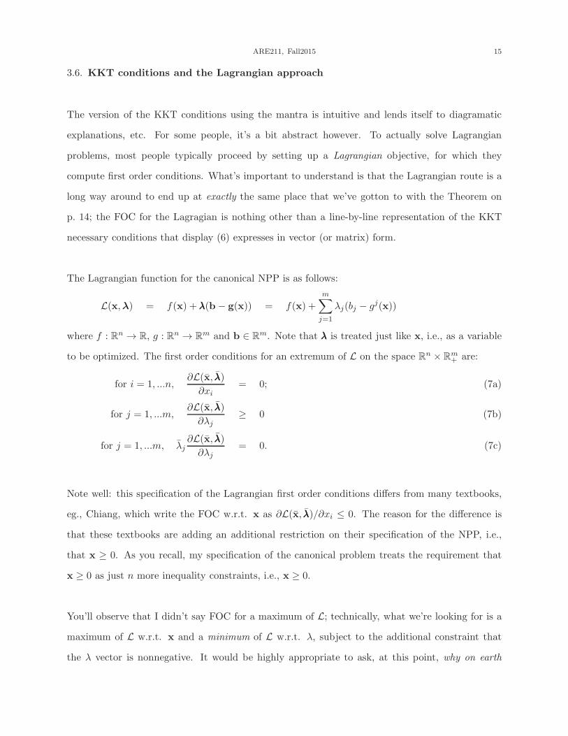
3.6. KKT conditions and the Lagrangian approach

The version of the KKT conditions using the mantra is intuitive and lends itself to diagramatic

explanations, etc. For some people, it’s a bit abstract however. To actually solve Lagrangian

problems, most people typically proceed by setting up a Lagrangian objective, for which they

compute first order conditions. What’s important to understand is that the Lagrangian route is a

long way around to end up at exactly the same place that we’ve gotton to with the Theorem on

p. 14; the FOC for the Lagragian is nothing other than a line-by-line representation of the KKT

necessary conditions that display (6) expresses in vector (or matrix) form.

The Lagrangian function for the canonical NPP is as follows:

L(x,λ) = f(x) + λλλ(b− g(x)) = f(x) +

m∑

j=1

λj(bj − gj(x))

where f : Rn → R, g : Rn → Rm and b ∈ R

m. Note that λλλ is treated just like x, i.e., as a variable

to be optimized. The first order conditions for an extremum of L on the space Rn × R

m+ are:

for i = 1, ...n,∂L(x, λλλ)

∂xi= 0; (7a)

for j = 1, ...m,∂L(x, λλλ)

∂λj≥ 0 (7b)

for j = 1, ...m, λj∂L(x, λλλ)

∂λj

= 0. (7c)

Note well: this specification of the Lagrangian first order conditions differs from many textbooks,

eg., Chiang, which write the FOC w.r.t. x as ∂L(x, λλλ)/∂xi ≤ 0. The reason for the difference is

that these textbooks are adding an additional restriction on their specification of the NPP, i.e.,

that x ≥ 0. As you recall, my specification of the canonical problem treats the requirement that

x ≥ 0 as just n more inequality constraints, i.e., x ≥ 0.

You’ll observe that I didn’t say FOC for a maximum of L; technically, what we’re looking for is a

maximum of L w.r.t. x and a minimum of L w.r.t. λ, subject to the additional constraint that

the λ vector is nonnegative. It would be highly appropriate to ask, at this point, why on earth


would anybody ever consider looking for such a weird object as a max w.r.t. x and a min w.r.t. λλλ

s.t. λλλ ≥ 0? It’s not highly intuitive. In fact, everybody always just talks about “the first order

conditions for the Lagrangian” and nobody bothers to wonder what it means, except in classes like

this. I strongly recommend not bothering to ask this highly appropriate question; instead, think

of the Lagrangian is nothing but a construction that delivers us the KTT conditions, i..e,

Theorem: A vector (x, λλλ) satisfies the KTT conditions (6) iff it satisfies (7)

To prove the theorem, recall the part of the KKT condition which states

▽f(x)T = λλλTJg(x) (6)

On the other hand, writing out ∂L(x,λλλ)∂xi

= 0, we have

∂f(x)

∂xi=

m∑

j=1

λj ·∂gj(x)

∂xi(8)

The left hand side of (8) is the i’th element of the vector ▽f(x). The right hand side is the inner

product of λλλ with the i’th row of the matrix Jg(x). Thus, the first order conditions for the xi’s are

simply a long-hand way of writing out what (6) states concisely in vector notation. Now consider

the m conditions on the λj ’s, i.e.,∂L(x,λλλ)

∂λj≥ 0, or bj ≥ gj(x). Taken together these m conditions

state that x belongs to the intersection of the lower contour sets of the gj ’s corresponding to the

bj ’s. Finally, consider the condition λj∂L(x,λλλ)

∂λj= 0, which is known as a complementary slackness

condition. This condition will be satisfied iff either λj = 0. or bj = gj(x) or both equalities are

satisfied simultaneously.

An important property of the Lagrangian specification is that the value of the Lagrangian function

at the solution to the NPP is equal to the maximized value of the objective function on the constraint

set. In symbols:

Theorem: At a solution (x, λλλ) to the NPP, L(x, λλλ) = f(x).

To see that this is correct note that L(x,λ) = f(x) + λλλ(b − g(x)). Each component of the inner

product λλλ(b− g(x)) is zero, since either (bj − gj(x)) is zero or λj is zero. Hence the entire second

term on the right hand side of the Lagrangian is zero.

ARE211, Fall2015 17

▽g1(x∗) ▽g2(x∗)

▽f(x∗)

constraint set

linearized constraint set

Figure 3. Varian’s “Hershey Kiss” example: the Constraint Qualification is violated

3.7. Role of the Constraint Qualification

We’ll now show that in the absence of the caveat about the constraint qualification, the KKT

theorem above would be false.

• the constraint qualification relates to the mysterious “bizarre exception” that is added as a

caveat to the mantra.

• In Fig. 3 below, the gradient vectors for the constraints satisfied with equality are not

linearly independent, and don’t span the domain of the objective function, so that you

can’t write the objective function as a linear combination of them. This doesn’t mean that

we don’t have a maximum at the tip of the constraint set.

• A sufficient condition for the CQ to be satisfied is that the gradients of the constraints

satisfied with equality at x form a linearly independent set.

• Another way of stating the above is as follows: let M(x) denote what’s left of Jg(x) (i.e.,

the Jacobian matrix of g evaluated at x), after you’ve eliminated all rows of this matrix

corresponding to constraints satisfied with strict inequality at x; a sufficient condition for

the CQ to be satisfied at x is that the matrix M(x) has full rank.

• If the constraint qualification isn’t satisfied then you could have a maximum at x but

wouldn’t know about it by looking at the KKT conditions. at this point.


• The right way to think about what goes wrong is that when the CQ is violated, the infor-

mation conveyed by the gradient vectors doesn’t accurately describe the constraint set.

• Saying this more precisely, when we use the KKT conditions to solve an NPP, what we are

actually doing is solving the linearized version of the problem. By this I mean, we replace

the boundary of the constraint set, as defined by the level sets of the constraint functions,

by the piecewise linear surface defined by the tangent planes to the level sets. In order for

the KKT conditions to do their job, it had better be the case that in a neighborhood of the

solution you are considering, this “linear shape” looks, locally, pretty much like the shape

of the true nonlinear constraint set for the problem.

• In the case of our example, the tangent lines to the two level sets, at the tip of the pointy

cone, are parallel to each other, so that the “linearized problem” is a line that goes on for

ever.

– Given the objective function that we’ve drawn, the linearized problem has no solution,

you just go on and on forever along the line.

– the constraint set for the true problem doesn’t look anything like a line, so that the

linearized problem is completely misleading

– observe that if you “bumped” the original problem a little bit, so that the tangent

planes at the tip were not parallel to each other, then the close relationship between

the original and the linearized problmes would be restored.

– what determines whether the linearized problem accurately represents the original

problem? Answer is apparent from comparing the relatinoship between the gradient

vectors to the tangent planes for the original, pathological problem to this relationship

for the bumped, well-behaved problem: in the former case, the two gradient vectors

are collinear.

– More generally, the linearized problem will locally accurately represent the original

nonlinear problem at a point if the gradient vectors of the constraints that are satisfied

with equality at that point form a linear independent set.

• You’ll notice that neither of the constraint functions are quasi-convex, and that the con-

straint set is not convex. A natural thing to hope is that imposing quasi-convexity of the

ARE211, Fall2015 19

▽g1(x∗) ▽g2(x∗)

▽f(x∗)

constraint set

linearized constraint set

Figure 4. An NPP with quasi-convex constraints which fails the CQ

constraint functions (convexity of the constraint set) would make this problem go away.

It doesn’t, as Fig. 4 illustrates: it’s a silly NPP problem because the constraint set is a

singleton. With some fiddling, however, we could easily fix that and make the constraint

set bigger.

It follows from the above that there are two special cases in which the constraint qualification is

satisfied vacuously.

(1) if all of the constraints are linear, (more precisely, if all of the constraint functions have affine

level sets). In this case, trivially, the linearized problem will be identical to the original

problem.

(2) if there is only one constraint, whose gradient is non-zero

It’s important to keep in mind that the constraint qualification is a sufficient condition that ensures

that the KKT conditions are necessary for a solution. Some people have wondered the following:

“could I find a point that satisfies the KKT conditions, leading me to believe that I’ve found a

solution to the NPP, but then the constraint qualification turns out to be violated, so that candidate

solution turns out not to be a solution?” The answer to this question is a resounding NO. If the

constraint qualification is violated, there may be solutions to the NPP that don’t satisfy the KKT

conditions.


If you say that finding a point that satisfies the KKT conditions is a “positive” and not finding

such a point is a “negative”, then we can talk about “false positives” (in the sense of a positive

result of a test, even though the thing you’re testing for (say pregnancy) hasn’t happened) and

“false negatives” (the test says you aren’t pregnant when you are).

In KKT theory, we’ve seen both kinds of “falseness”: there are several ways that we can get “false

positives” in the sense that the KKT conditions are satisfied at some point which does not solve the

NPP. We’ll see some of these in a minute. However, provided your function is differentiable and

the constraint set is compact, the only way to get a “false negative” is for the CQ to be violated

(e.g., Varian’s “Hershey Kiss” example (Fig. 3 below)). Thus, provided the CQ is not violated,

there will be no “false negatives” and the maximum (if it exists) must satisfy KKT.

3.8. Binding constraints vs constraints satisfied with equality

In some math-for-economists text-books (e.g., Simon and Blume), the term “constraint satisfied

with equality” is (unfortunately) replaced by “binding constraints”. This is unfortunate because

in practice, economists almost always reserve the term “binding” for a subclass of the constraints

satisfied with equality. Specifically, a constraint is said to be binding if the maximized value of the

objective function increases when the constraint is relaxed a little bit. (A constraint is relaxed by

increasing the constant on the right hand side of the constraint inequality.) For example in Fig. 5,

both constraints are satisfied with equality, but only g1 is binding; if you relax constraint g1 (left

panel of Fig. 6) the optimum moves to the north-east; if you relax constraint g2 (right panel of

Fig. 6) , the solution is unchanged.

Formally, consider the problem

max f(x) s.t. g(x) ≤ b

Let µ(b) denote the solution to the problem with constraint vector b. We now say that constraint

j is binding if there exists ǫ > 0 such that ∀ǫ ∈ (0, ǫ), µ(b+ ǫej) > µ(b), where ej denotes the j’th

unit vector. In this course we’ll always say that a constraint is “satisfied with equality” unless we

know that it’s actually binding in the sense above.

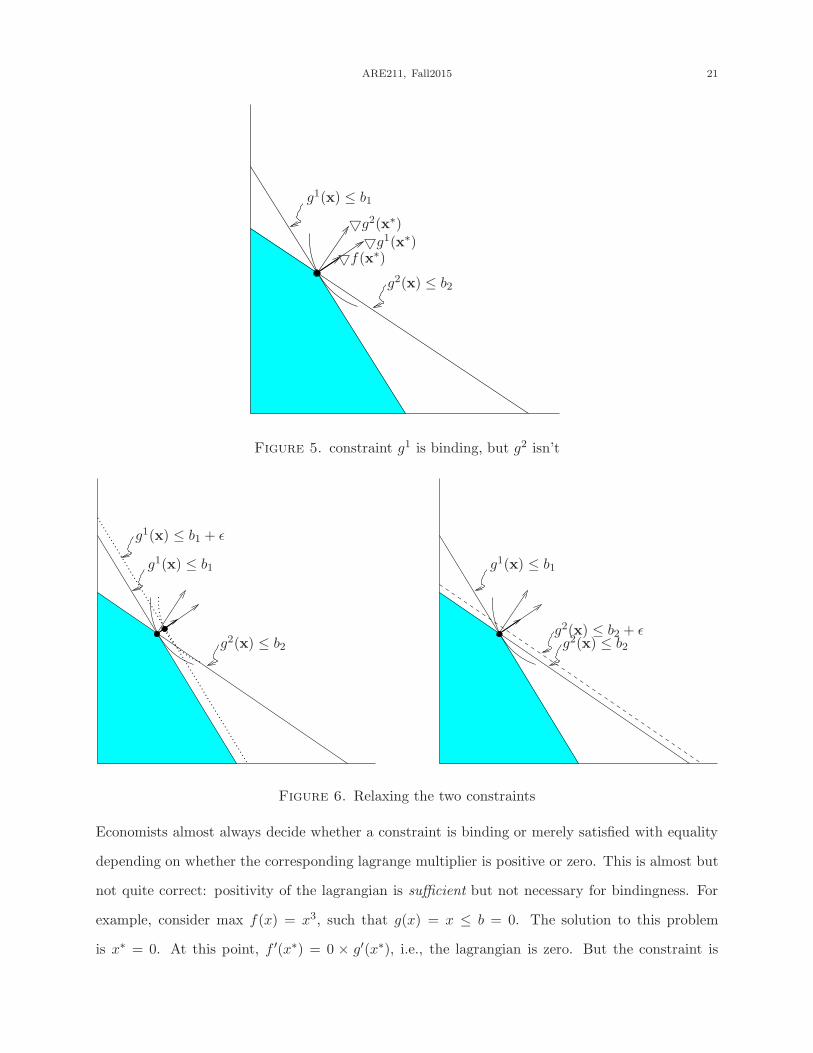
ARE211, Fall2015 21

g1(x) ≤ b1

g2(x) ≤ b2

▽g1(x∗)

▽g2(x∗)

▽f(x∗)

Figure 5. constraint g1 is binding, but g2 isn’t

g1(x) ≤ b1

g1(x) ≤ b1 + ǫ

g2(x) ≤ b2

g1(x) ≤ b1

g2(x) ≤ b2g2(x) ≤ b2 + ǫ

Figure 6. Relaxing the two constraints

Economists almost always decide whether a constraint is binding or merely satisfied with equality

depending on whether the corresponding lagrange multiplier is positive or zero. This is almost but

not quite correct: positivity of the lagrangian is sufficient but not necessary for bindingness. For

example, consider max f(x) = x3, such that g(x) = x ≤ b = 0. The solution to this problem

is x∗ = 0. At this point, f ′(x∗) = 0 × g′(x∗), i.e., the lagrangian is zero. But the constraint is


certainly binding. We’ve seen this distinction over and over again in this course. What’s going on

here is exactly the same as what’s going on when we say that negative definiteness of the Hessian

is sufficient but not necessary for strict concavity.

3.9. Interpretation of the Lagrange Multiplier

The Lagrangian λj has an interpretation that proves to be important in a wide variety of economic

applications.

• it is a measure of how much bang for the buck you get when you relax the j’th constraint.

That is, if you increase bj by one unit, then the maximized value of your objective function

will go up by λj units.

• Example: think of maximizing utility on a budget constraint. the higher are prices the

longer is the gradient vector, and so the shorter is λ, i.e., the less bang for the buck you get,

literally. I.e., relaxing your budget constraint by a dollar doesn’t by much more of a bundle,

so that your utility can’t go up by much. On the other hand, for a fixed price vector, the

length of the gradient of your utility function is a measure of how easy to please you are.

If you are a kid who gets a lot of pleasure out of penny candy, then relaxing the budget

constraint by a dollar will buy you a lot.

• the importance of this in economic applications is that you often want to know what the

economic cost of a constraint is, e.g., suppose you are maximizing output subject to a

resource constraint: what’s it worth to you to increase the level of available resources by

one unit. Get answer by looking at the Lagrangian.

• The mathematical proof is as usual completely trivial. Let M(b) denote the maximized

value of the objective function when the constraint vector is b.

M(b) = f(x(b)) = L(x(b), λλλ(b)) = f(x) + λλλ(b− g(x)).

ARE211, Fall2015 23

we have

dM(b)

dbj=

dL(x(b), λλλ(b))

dbj=

n∑

i=1

{

fi(x(b)) −

m∑

k=1

λkgki (x(b))

}

dxidbj

+m∑

k=1

dλk

dbj(bk − gk(x)) + λj

– For each i, the term in curly brackets is zero, by the KKT conditions.

– For each k,

∗ If (bk − gk(x)) = 0, then dλk

dbj(bk − gk(x)) is zero.

∗ If (bk − gk(x)) < 0, then λk(·) will be zero on a neighborhood of b, so that

dλk(·)dbj

= 0.

– The only term remaining is λj .

– Conclude that dM(b)dbj

= λj

• Here’s a more intuitive approach for the case of a single binding constraint.

– increase the constraint b to b+ db.

– you should respond by moving from solution x in the direction of steepest ascent, i.e.,

in the direction that the gradient is pointing.

– move from x in the direction that ▽f(x) is pointing until you reach the new constraint,

i.e., define dx by g(x+ dx) = b+ db. Now initially we had g(x) = b. Hence

db = g(x + dx)− g(x) ≈ ▽ g(x)dx

while

df = ▽ f(x)dx

which by the KKT conditions

= λ▽ g(x)dx

Hence

df = λdb


Hence (being a little fast and loose with infinitesimals), df/db = λ.

Note that λ will be larger

• the more rapidly f increases with x (i.e., the longer is the vector ▽f(x)).

• the less rapidly g increases with x (i.e., the shorter is the vector ▽g(x)).

Note also that the above “proves” the 2nd part of the mantra, i.e., if constraint j is satisfied with

equality but is not binding, then the weight on this constraint must be zero when you write ▽f(x)

as a nonnegative linear combination of the ▽gj(x)’s. The following argument proves this rather

sloppily: (a) if constraint j is satisfied with equality but is not binding, then by definition dfdbj

= 0;

(b) since dfdbj

= λj , then λj must be zero.

Fig. 7 illustrates what’s going on. In the left panel,

• || ▽ f || is small and || ▽ g|| is big;

• since || ▽ g|| is big, only a small dx is required in order to increase g by one unit.

• since || ▽ f || is small, this small dx increases f by only a little bit.

In the right panel, everything is reversed:

• || ▽ g|| is small and || ▽ f || is big;.

• Since || ▽ g|| is small, a big dx is required in order to increase g by one unit.

• Since || ▽ f || is big, this big dx increases f by a lot.

3.10. Demonstration that KKT conditions are necessary

Rather than prove the result generally, we are just going to look at special cases. Throughout this

subsection, we are going to ignore the question of whether the KTT conditions are sufficient for a

solution. The pictures we are going to consider are of functions so well behaved that if the KTT

conditions are satisfied at a point then that point is a solution.

The case of one inequality constraint: With one constraint, the picture is easy: the condition is

ARE211, Fall2015 25

g(x∗) = b+ 1 (g ↑↑ given dx)

g(x∗) = b

▽g(x∗)

▽f(x∗)

f(·) = f(x∗)f(·) = f(x∗) + small ∆f

λ = ||▽f(x∗)||||▽g(x∗)|| is small

g(x∗) = b+ 1 (g↑ given dx)

g(x∗) = b

▽f(x∗)

▽g(x∗)

f(·) = f(x∗)

f(·) = f(x∗) + BIG ∆f

λ = ||▽f(x∗)||||▽g(x∗)|| is big

Figure 7. Interpretation of the Lagrangian

in same

point

direction

arrows

constraint arrow

objective arrow

Lower contour set of g

corresponding to b

y

x1

x2

g(x) = b

x1

x2

x3

Figure 8. Constrained max problem with one inequality constraint

that ▽f(x) = λ ▽ g(x), for some nonnegative scalar λ. Also, with one constraint the CQ is

vacuous. In Fig. 8


• The constraint is the condition that g(x) ≤ b. That is, the only x’s we are allowed to

consider are x’s for which the function g assigns values weakly less than b.

• Three candidates in the picture x1, x2 and x3. Each curve represents a level set of some

function thru one of these points. Note: each level set belongs to a different function!

• Point x2 isn’t a maximum; upper contour set intersects with constraint set; Point x3 isn’t

either. Point x1 is the only one with the property that there’s nothing in the strict upper

contour set that is also in the constraint set.

• Now put in the arrows. Call the first the objective arrow (i.e., the gradient of the objective

function) and the second the constraint arrow (i.e., the gradient of the constraint function).

Which way do the objective arrows point?

– arrow points in direction of increase

– this must be the upper contour set

– upper contour set is convex

– Conclude: we know that the arrow for a level set points into the corresponding upper

contour set, which for a quasi-concave function is the convex set bounded by the set.

• Which way does the constraint arrow point? Must be NE because the lower contour set is

SW.

• Now characterize the condition for a maximum in terms of the arrows. Answer is that

arrows lie on top of each other and point in the same direction (as opposed to lying on top

of each other but point at 180 degrees to each other).

• Conclude in terms of the mantra: arrow lies in the positive cone defined by the unique

binding constraint.

Question: Suppose that for each of the level sets of f , the gradient vector at every point on this

level set points SW as in point x3? What can you conclude about the solution to the maximization

problem?

ARE211, Fall2015 27

▽g1

▽g2

▽f

dx

θ(dx,▽f) < 90◦

θ(dx,▽g2) > 90◦

Figure 9. Graphical Illustration of the KKT conditions: two constraints

Answer: There is no solution. Certainly there can’t be a solution in which the constraint is

binding. And there can’t be an unconstrained solution either. You can always move a bit further

southwest and increase the value of f

More formally, for the case of one inequality constraint, the KKT condition is that there is a

nonnegative collinear relationship between the gradients of the objective and the constraint func-

tions. To see that this condition is necessary, suppose you don’t have nonnegative collinearity, i.e.,

▽f(x) is not a nonnegative scalar multiple of ▽g(x). Then you can find a vector dx such that

▽g(x) · dx < 0 and ▽f(x) · dx > 0. (Takes a bit of linear algebra work to prove this but it’s

obvious diagramatically.) But this means that x + dx satisfies the inequality constraint and (by

Taylor’s theorem) increases f provided dx is sufficiently small.

The two constraint case: With two constraints the condition says that at the solution the gradient

vector ▽f(x), can be written as a nonnegative linear combination of the gradients of the constraints

that are satisfied with equality

What does this mean geometrically:


• means that the gradient vector of the objective function points into the cone defined by the

gradients of the constraints that are satisfied with equality. Go over what it means for a

vector to be inside the positive cone defined by two others. Show geometrically that if a

vector x is inside the cone, you can take positive scalar multiples of the vectors that define

the cone, and reconstruct x. Otherwise, you can’t reconstruct x with positive coefficients.

• to see why must this condition hold geometrically, we draw a picture (Fig. 9) that has only

the gradients drawn in (none of the constraint sets or indifference curves will be drawn in)

and argue from the vectors alone why the above condition is necessary.

• Suppose the above condition is violated, so that ▽f(x) lies outside the cone defined by the

gradients of the constraints that are satisfied with equality. Clearly, we can then draw a line

(the horizontal dotted line in Fig. 9) such that the gradient vectors of all of the constraints

lie on one side of the line, and the gradient vector of the objective function lies on the other

side. (Again this is obvious geometrically, but requires some work to prove rigorously.)

• We can now draw a vector dx that makes an acute angle with ▽f(x) but an obtuse angle

with all of the constraint vectors. We can always do this: make dx arbitrarily close to the

line perpendicular to the first dotted line, which ensures that dx will make an obtuse angle

with the constraint gradients, but must make an acute angle with ▽f(x) since both vectors

are trapped within the quadrant defined by the dotted lines.

• Observe that it makes an obtuse angle with all of the constraint vectors.

• Reason from there:

– add dx to x

– observe that f(x+ dx)− f(x) ≈ ▽f(x) · dx > 0;

– i.e., moving in this direction increases the objective function.

– similarly, for all j such that the j’th constraint is satisfied with equality, observe that

gj(x + dx) − gj(x) ≈ ▽gj(x) · dx < 0, i.e., reduces the value of all of the constraints

that are satisfied with equality.

– for j’s that aren’t, if dx is sufficiently small, then you can increase the value of gj(·) a

little bit and still be less than bj.

ARE211, Fall2015 29

Lower contour set of g corresponding to b

Upper contour set of g corresponding to b

x1

x2

g(x) = b

x1

x2

x3

▽g(x)

▽f(x)

▽f(x)

−▽ g(x)

Figure 10. Maximization subject to an equality constraint

– in other words, you can move a little in the direction of dx and stay within the

constraint set, yet increase the value of f .

– This establishes that x couldn’t have been a maximum.

3.11. KKT conditions with equality constraints

One equality constraint, g(x) = b: Consider the problem

max f(x) subject to g(x) = b;

• This is a much more restrictive problem than the corresponding problem with inequality

constraints:

– in this problem the solution has to belong to the level set of g(·) corresponding to b.

– if the constraint were an inequality, x could be anywhere in the lower contour set of

g(·) corresponding to b.

• as the picture illustrates

– it’s still the case that a necessary condition for x to solve the problem is that ▽f(x)

and ▽g(x) are colinear


– but in this problem, it’s possible for ▽g(x) to be a negative scalar multiple of ▽f(x).

∗ in this case, the ▽f(x) would point into the lower contour set of g corresponding

to b.

– in other words, the nonnegativity constraint on λ no longer applies.

– the necessary condition is now

▽f(x) = λ▽ g(x), λ ∈ R

In terms of the mantra, we replace the term “nonnegative cone” with “subspace”.

Multiple equality constraints: g(x) = b:

The KKT conditions for equality constrained problems: Mantra format:

(Except for a bizarre exception) a necessary condition for x to solve a constrained maximization

problem in which all constraints must hold with equality is that the gradient vector of the objective

function at x belongs to the subspace defined by the gradient vectors of the constraints that are

satisfied with equality at x.

The KKT conditions for pure equality constrained problems: math format:

maximize f(x) subject to g(x) = b,

where f : Rn → R and g : Rn → Rm

If x solves the maximization problem and the constraint qualification holds at x then there exists

a vector λλλ ∈ Rm such that

▽f(x)T = λλλTJg(x)

Equality and Inequality constraints

The KKT conditions for problems with equality and inequality constraints: math format:

maximize f(x) subject to g1(x) ≤ b1,g2(x) = b2 where f : Rn → R and gi : Rn → Rmi

ARE211, Fall2015 31

If x solves the maximization problem and the constraint qualification holds at x then there exists

vectors λλλ1 ∈ Rm1

+ , λλλ2 ∈ Rm2

such that

▽f(x) = λλλ1Jg1(x) + λλλ2Jg2(x)

Moreover, λλλ1 has the property that λ1j = 0, for each j such that g1j (x) < b1j .

contents n - university of california, berkeley · pdf filecontents 3. nonlinear ... kkt...

Documents