civil engineering department - cive 711 · cive 711 - dr. t. hegazy 4 cive 711- current research...

CIVE 711 - Dr. T. Hegazy 1

Civil Engineering Department - CIVE 711

CIV E 711 - COMPUTER-AIDED PROJECT ORGANIZATION & MANAGEMENT Instructor: Dr. Tarek Hegazy, CPH 2369CG, Ext.: 32174, E-mail: [email protected]

Description: Application of traditional and Artificial Intelligence-based computerized tools for effectively managing the time, money, and resources of projects. It covers: review of the CPM method, project management software, optimization using Excel Solver, Expert Systems, Neural Networks, OOP programming, Genetic Algorithms, Fuzzy Logic, integrated project management tools, Asset Management Systems, various case studies and hands-on computer workshops. The course involves assignments, computer workshops, a project, and a final examination. Suggested Texts: (1) Hegazy 2002, “Computer-Based Construction Project Management,” Prentice Hall. (2) Negnevitsky, M. 2005 “Artificial Intelligence” A guide to intelligent systems, 2nd Ed., Addison Wesley. (3) Hendrickson, C. and Au, T. “Project management for Construction: Fundamental Concepts for

Owners, Engineers, Architects, and Builders,” Prentice Hall, 1989. (4) Ahuja, H.N. “Construction Performance Control by Networks,” John Wiley & Sons, 1976. (5) Clough, R.H. and Sears, E. “Construction Project Management,” Second Edition, John Wiley &

Sons, Toronto, 1979.

Tentative Content: Week Subject

1 • Introduction to Project Management.2 • Optimization using Excel Solver.3 • EasyPlan & Microsoft Project Software. 4 • Genetic Algorithms.5 • AI & Expert Systems.6 • Neural Networks. 7 • Fuzzy Logic.8 • Hybrid AI tools.9 • Asset Management.10 • Planning of repetitive projects.11 • Project control techniques & Earned-12 • Class presentations.


References on Project Management:

• Books on Project Management and Construction Management;

• Trade magazines (e.g., ENR);

• International journals such as:

o Construction Engineering and Management (ASCE);

o Computing in Civil Engineering (ASCE);

o Infrastructure Systems (ASCE);

o Computer-Aided Civil and Infrastructure Engineering;

o Automation in Construction;

o Cost Engineering (AACE);

o Construction Management and Economics;

o Knowledge-Based Systems;

o Quality in Maintenance & Engineering; and

o Computers in Industry.

• Databases such as "current contents" , "compendex" & "CISTI";

• International organizations such as Project Management Institute (PMI) and American Association of Cost Engineers (AACE);

• A lot of computer software programs;

• Internet search;

• News groups; and

• Government publications such as statistics Canada, etc.


Interesting Project Management Proverbs:

- If you fail to plan, you plan to fail.

- There are no good project managers - only lucky ones. The more you plan the luckier you get.

- Fast - cheap - good: you can have any two, not all three.

- Be realistic. If it takes 1 person 1 hour to go to Toronto, it does not take half an hour from 2 people.

- The person who says it will take the longest and cost the most is the most knowledgeable.

- The most valuable and least used WORD in a project manager's vocabulary is "NO".

- The most valuable and least used PHRASE in a project manager's vocabulary is "I don't know".

- If it happens once it's ignorance, if it happens twice it's neglect, if three times it's policy.

- You can get someone to commit to a strict deadline, but you cannot get him into meeting it.

- A badly planned project will take three times than expected - a well planned project only twice.

- The sooner you get behind schedule, the more time you have to make it up.

- A problem shared is a buck passed.

- Of several possible interpretations of a communication, the least convenient is the correct one.

- If everything is going exactly to plan, something somewhere is going massively wrong.

- Project management tools are used most for predicting, not preventing, cost & schedule overruns.

- For a project manager, overruns are as certain as death and taxes.

- Some projects finish on time in spite of project management best practices.

- When the project’s paperwork weighs as much as the project itself, the project is complete.

- If you can interpret project status in several different ways, the most painful will be correct.

- A project ain't over until the fat cheque is cashed.

- No project has ever finished on time, within budget, to requirement - yours won't be the first.

- Good control reveals problems early - which means you'll have longer to worry about them.

- If it can go wrong, it will - Murphy's Law.

- Work expands to fill the time available for its completion - Parkinson's Law.

- The common 7 phases of a project are: Wild enthusiasm; Disillusionment; Confusion; Panic; Search

for the guilty; Punishment of the innocent; and Promotion of non-participants.


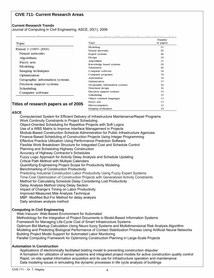
CIVE 711- Current Research Areas

Current Research Trends Journal of Computing in Civil Engineering, ASCE, 20(1), 2006 Titles of research papers as of 2005 ASCE

Computerized System for Efficient Delivery of Infrastructure Maintenance/Repair Programs Work Continuity Constraints in Project Scheduling Object-Oriented Scheduling for Repetitive Projects with Soft Logics Use of a WBS Matrix to Improve Interface Management in Projects Module-Based Construction Schedule Administration for Public Infrastructure Agencies Finance-Based Scheduling of Construction Projects Using Integer Programming Effective Practice Utilization Using Performance Prediction Software Flexible Work Breakdown Structure for Integrated Cost and Schedule Control Planning and Scheduling Highway Construction Accuracy of Highway Contractor’s Schedules Fuzzy Logic Approach for Activity Delay Analysis and Schedule Updating Critical Path Method with Multiple Calendars Quantifying Engineering Project Scope for Productivity Modeling Benchmarking of Construction Productivity Predicting Industrial Construction Labor Productivity Using Fuzzy Expert Systems Time-Cost Optimization of Construction Projects with Generalized Activity Constraints Method for Calculating Schedule Delay Considering Lost Productivity Delay Analysis Method Using Delay Section Impact of Change’s Timing on Labor Productivity Improved Measured Mile Analysis Technique MBF: Modified But-For Method for delay analysis Daily windows analysis method

Computing in Civil Engineering

Web-Vacuum: Web-Based Environment for Automated Methodology for the Integration of Project Documents in Model-Based Information Systems Framework for Managing Life-Cycle Cost of Smart Infrastructure Systems Optimum Bid Markup Calculation Using Neuro fuzzy Systems and Multidimensional Risk Analysis Algorithm Modeling and Predicting Biological Performance of Contact Stabilization Process Using Artificial Neural Networks Building Project Model Support for Automated Labor Monitoring Parallel Computing Framework for Optimizing Construction Planning in Large-Scale Projects

Automation in Construction

Applications of electronically facilitated bidding model to preventing construction disputes A formalism for utilization of sensor systems and integrated project models for active construction quality control Rapid, on-site spatial information acquisition and its use for infrastructure operation and maintenance Data modeling issues in simulating the dynamic processes in life cycle analysis of buildings


Content-Based Search Engines for construction image databases Object-oriented framework for durability assessment and life cycle costing of highway bridges Dynamic planning and control methodology for strategic and operational construction project management Planning gang formwork operations for building construction using simulations Application of integrated GPS and GIS technology for reducing construction waste and improving construction efficiency Maintenance optimization of infrastructure networks using genetic algorithms A computer-based scoring method for measuring the environmental performance of construction activities Model-based dynamic resource management for construction projects 4D dynamic management for construction planning and resource utilization PPMS: a Web-based construction Project Performance Monitoring System Automated project performance control of construction projects A cooperative Internet-facilitated quality management environment for construction A process-based quality management information system System development for non-unit based repetitive project scheduling Simulation-based optimization for dynamic resource allocation A WICE approach to real-time construction cost estimation

Construction Management and Economics

Integrated maintenance management of hospital buildings: a case study Web-based integrated project control system Service quality performance of design/build contractors using quality function deployment Safety and production: an integrated planning and control model Trends of 4D CAD applications for construction planning An integrated construction project cost information system using MS Access and MS Project Production arrangements by US building and non-building contractors: an update A typology for clients' multi-project environments Combining various facets of uncertainty in whole-life cost modeling Grey relation analysis of causes for change orders in highway construction Development of a model to estimate the benefit-cost ratio performance of housing Scheduling system with focus on practical concerns in repetitive projects Managing knowledge: lessons from the oil and gas sector Simulation of maintenance costs in UK local authority sport centers Project management decisions with multiple fuzzy goals Service life prediction of exterior cladding components under standard conditions Documentation, standardization and improvement of the construction process in house building Innovative construction technology for affordable mass housing in Tanzania, East Africa Selection of vertical formwork system by probabilistic neural networks models Project cost estimation using principal component regression Using linear model for learning curve effect on highrise floor construction Accelerating linear projects Predicting the risk of contractor default in Saudi Arabia utilizing artificial neural network (ANN) and genetic algorithm (GA) techniques Forecasting the residual service life of NHS hospital buildings: a stochastic approach Using the principal component analysis method as a tool in contractor pre qualification The JIT materials management system in developing countries Use of information and communication technologies by small and medium sized enterprises (SMEs) in building construction Identifying management research priorities A linear discrete scheduling model for the resource constrained project scheduling problem Justification time management in the ready mixed concrete industries of Chongqing, China and Singapore A model for automated monitoring of road construction Improvement tools in the UK construction industry Time series forecasts of the construction labour market in Hong Kong: the Box Jenkins approach


Basics of Scheduling


Another Example


CIVE 711 – Scheduling Assignment 1. For the following project:

A. Manually draw the logic network and identify the critical path. B. Manually draw a “late” bar chart. C. What is the effect of delaying activity G by 6 days? D. Enter the project into EasyPlan, print the schedule, the network, and the cash flow chart.

Activity

Predecessors Duration (days)

Cost (x$1000)

A B C D E F G H I J

---- A A A B D B C, E F G, H, I

4 6 4 9 3 8 10 2 4 2

5 3 4 2 4 5 2 2 4 3

2. Manually calculate the schedule for the following network. Enter the data into Microsoft Project and

print the resulting schedule. 3. In EasyPlan, use the “Web Tutorial” and load Pr7 (as discussed in the project management article).

Solve the exercise and print your score and the optimum schedule. Note that the part of dealing with actual progress data is not part of the assignment.

A

8

4

E

6

C

6

Y

4

X

2

Overlap between finish of X & start of Y

3

Activity duration (Overlaps and durations in days)

TF= TF=

2 5

K

4 TF=

H

7TF=

F

8TF=

D

8 TF=

B

7 TF=

J

3TF=

I

9TF=

TF= G

6TF=

Activity


Introduction to Artificial Intelligence

-Take a minute to calculate the following manually: 45.32 (98.2 x123.59)12 / 27.2 = ? If not done, give it to a cheap $1 calculator. Who is smart now? - Consider the example of O.J. Simpson’s Trial and the conflicting evidence. How did the jury and judge make a decision? Can the judge explain the logic? Was any calculation involved? How much time needed? - Can you guess the age of this person by looking at the picture for only 2 seconds? Was any calculation involved? Can you explain your logic? Can your computer do that?

************************************************************ Can you read this ?

can uoy blveiee taht I cluod auclaly uesdnatnrd waht I was redanieg. The

phaonmneal pweor of the hmuan mnid, aoccdrnig to a rscheearch at Cmabrigde

Uinervtisy, it deosn't mttaer in waht oredr the ltteers in a wrod are, the olny

iprmoatnt thing is taht the frist and lsat ltteer be in the rghit pclae. The rset can be

a taotl mses and you can sitll raed it wouthit a porbelm. Tihs is bcuseae the huamn

mnid deos not raed ervey lteter by istlef, but the wrod as a wlohe. Amzanig huh?

Yaeh and I awlyas tghuhot slpeling was ipmorantt!

************************************************************ Who has more processing power: A supercomputer or the brain of a fly? Who is more intelligent? How to add intelligence to computers?


Solving Optimization Problems: Evolutionary Systems? Compromise between Local versus Global search strategies.


Optimization Using Excel Solver

Solve the following two questions using Excel Solver Question 1: A concrete manufacturer is concerned about how many units of two types of concrete elements should be produced during the next time period to maximize profit. Each concrete element of type I generates a profit of $60, while each element of type II generates a profit of $40. 2 and 3 units of raw materials are needed to produce one concrete element of type I and II, respectively. Also, 4 and 2 units of time are required to produce one concrete element of type I and II, respectively. If 100 units of raw materials and 120 units of time are available, how many units of each type of concrete element should be produced to maximize profit and satisfy all constraints? Use Excel solver for the solution.

Question 2: A building contractor produces two types of houses: detached and semidetached. The customer is offered several choices of architectural design and layout for each type. The proportion of each type of design sold in the past is shown in the following table. The profit on a detached house and a semidetached house is $1,000 and $800 respectively.

Design Detached Semidetach

ed Type A Type B Type C

0.1 0.4 0.5

0.33 0.67 -----

The builder has the capacity to build 400 houses per year. However, an estate of housing will not be allowed to contain more than 75% of the total housing as detached. Furthermore, because of the limited supply of bricks available for type B designs, a 200-house limit with this design is imposed. Use Excel to develop a model of this problem and then use SOLVER to determine how many detached and semidetached houses should be constructed in order to maximize profits. State the optimum profit.


Example on Genetic Algorithms Problem: A square construction site is divided into 9 grid units. We need to use GAs to determine the best

location of two temporary facilities A and B, so that:

- Facility A is as close as possible to facility B. - Facility A is as close as possible to the fixed facility F. - Facility B is as far as possible to the fixed facility F.

Step 1: Problem Representation (how to define a facility location) Option 1 Option 2 Using coordinates Using location index A has X = 2 and Y = 1 A is in Location index 2 B has X = 1 and Y = 3 B is in Location index 7 Step 2: Chromosome Structure The variables in our problem are the locations of facilities A & B. Then, the chromosome structure for each of the two options in Step 1 are as follows. Note that the genes of a chromosome are the variables. 4 Genes 2 Genes (Values range from 1 to 3) (Values range from 1 to 8) Step 3: Generate Population (50 to 100 is reasonable diversity & processing time) (note: for this exercise, let’s consider option 1 representation and a population of 3) P1 P2 P3

A B F

x

y

A B F

1 2 3

4 5 6

7 8 9

XA

YA

XB YB

2 1 1 3

Index A

Index B

2 7

XA

YA

XB YB

1 1 3 2

XA

YA

XB YB

2 1 1 3

XA

YA

XB YB

1 3 2 2

A B F

A B F

B A F


Step 4: Evaluate the Population P1 P2 P3 Objective function = Minimize site score = Minimum of ∑ d . W

Score = dAB . WAB + dAF . WAF + dBF . WBF

Let’s consider the closeness weights (W) as follows (from past notes): WAB = 100 (positive means A & B close to each other) WAF = 100 (A & F close to each other) WBF = -100 (negative means B & F far from each other)

Let’s also consider the distance (d) between two facilities as the number of horizontal and vertical blocks between them.

P1 Score = dAB . WAB + dAF . WAF + dBF . WBF = 3 . 100 + 4 . 100 + 1 . -100 = 600 P2 Score = dAB . WAB + dAF . WAF + dBF . WBF = 3 . 100 + 3 . 100 + 2 . -100 = 400 P3 Score = dAB . WAB + dAF . WAF + dBF . WBF = 2 . 100 + 2 .100 + 2 . -100 = 200

Step 5: Calculate the Merits of Population Members Merit of P1 = (600+400+200) / 600 = 2 Merit of P2 = (600+400+200) / 400 = 3 Merit of P1 = (600+400+200) / 200 = 6 Notice the sum of merits = 11

Notice that smaller score gives higher merit because we are interested in minimization. In case of maximization, we use the inverse of the merit calculation.

Step 6: Calculate the Relative Merits of Population Members RM of P1 = merit * 100 / Sum of merits = 2 . 100 / 11 = 18 RM of P2 = merit * 100 / Sum of merits = 3 . 100 / 11 = 27 RM of P3 = merit * 100 / Sum of merits = 6 . 100 / 11 = 55 Step 7: Randomly Select Operator (Crossover or Mutation) Crossover rate = 96% (marriage is the main avenue for evolution)

Mutation rate = 4% (genius people are very rare) To select which operator to use in current cycle, we generate a random number (from 0 to 100). If the value is between 0 to 96, then crossover, otherwise, mutation. Step 8: Use the Selected Operator (Assume Crossover)

A B F

A B F

B A F


8.a) Randomly select two parents according to their relative merits of Step 6 0 18 45 100 Relative merits on a cumulative horizontal scale. For first parent, we generate a random number (0 to 100). According to its value, we pick the parent. For example, assume value is 76, then P3 is selected. For the 2nd parent, get a random number (0 to 100). Assume 39, Then P2 is picked. 8.b) Let’s apply crossover to generate an offspring P3 P2 Step 9: Evaluate the Offspring Offspring 1

Notice that Offspring 2 is invalid because both facilities A & B are at same coordinates (x = 2 and Y = 3) and this is not allowed

Offspring Score = dAB.WAB + dAF.WAF + dBF.WBF = 1.100 + 4.100 + 3. -100 = 200 Step 10: Compare the Offspring with the Population (Evolve the Population) Since the offspring score = 200 is better than the worst population member (P1 has a score of 600), then the offspring survives and P1 dies (will be replaced by the offspring).

Accordingly, P1 becomes:

At the end of this step, we GOTO STEP 4 , repeating the process thousands of times until the best solution is determined. One of the top solutions is as follows:

Score = 0

P1 P2 P3

2 1 1 3

1 3 2 2

2 3 2 3

1 1 1 2 For the crossover

range, we get 2 random numbers, say 2 and 3

Offspring 1 Offspring 2 (Invalid)

A B F

B A F

1 1 1 2


Comparison among five evolutionary-based optimization algorithms by

Emad Elbeltagi; Tarek Hegazy; and Donald Grierson

ABSTRACT: Evolutionary algorithms are stochastic search methods that mimic the natural biological evolution and/or the social behavior of species. Such algorithms have been developed to arrive at near-optimum solutions to large-scale optimization problems, for which traditional mathematical techniques may fail. This paper compares the formulation and results of five recent evolutionary-based algorithms: genetic algorithms, memetic algorithms, particle swarm, ant colony systems, and shuffled frog leaping. A brief description of each algorithm is presented along with a pseudocode to facilitate the implementation and use of such algorithms by researchers and practitioners. Benchmark comparisons among the algorithms are presented for both continuous and discrete optimization problems, in terms of processing time, convergence speed, and quality of the results. Based on this comparative analysis, the performance of evolutionary algorithms is discussed along with some guidelines for determining the best operators for each algorithm. The study presents sophisticated ideas in a simplified form that should be is beneficial to both practitioners and researchers involved in solving optimization problems. 1. Introduction The difficulties associated with using mathematical optimization on large scale engineering problems have contributed to the development of alternative solutions. Linear programming and dynamic programming techniques, for example, often fail (or reach local optimum) in solving NP-hard problems with large number of variables and non-linear objective functions [1]. To overcome these problems, researchers have proposed evolutionary-based algorithms for searching near-optimum solutions to problems. Evolutionary Algorithms are stochastic search methods that mimic the metaphor of natural biological evolution and/or the social behavior of species. Examples include how ants find the shortest route to a source of food and how birds find their destination during migration. The behaviour of such species is guided by learning, adaptation, and evolution [1]. To mimic the efficient behaviour of these species, various researchers have developed computational systems that seek fast and robust solutions to complex optimization problems. The first evolutionary-based technique introduced in the literature was the Genetic Algorithms, [2]. Genetic Algorithms (GAs) were developed based on the Darwinian principle of the “survival of the fittest” and the natural process of evolution through reproduction. Based on its demonstrated ability to reach near-optimum solutions to large problems, the GAs technique has been used in many applications in science and engineering [e.g.,3,4,5]. Despite their benefits, GAs may require long processing time for a near-optimum solution to evolve. Also, not all problems lend themselves well to a solution with GAs [6]. In an attempt to reduce processing time and improve the quality of solutions, particularly to avoid being trapped in local optima, other Evolutionary Algorithms (EAs) have been introduced during the past 10 years. In addition to various GA improvements, recent developments in EAs include four other techniques inspired by different natural processes: memetic algorithms [7], particle swarm optimization [8], ant colony systems [9], and shuffled frog leaping [10]. A schematic diagram of the natural processes that the five algorithms mimic is shown in Fig. 1. In this paper, the five EAs presented in Fig. 1 are reviewed and a pseudocode for each algorithm is presented to facilitate its implementation. Performance comparison among the five algorithms is then presented. Guidelines are then presented for determining the proper parameters to use with each algorithm. 2. Five evolutionary algorithms In general, EAs share a common approach for their application to a given problem The problem first requires some representation to suit each method. Then, the evolutionary search algorithm is applied iteratively to arrive at a near-optimum solution. A brief description of the five algorithms is presented in the following subsections.

2.1. Genetic algorithms Genetic algorithms (GAs) are inspired by biological systems’ improved fitness through evolution [2]. A solution to a given problem is represented in the form of a string, called “chromosome”, consisting of a set of elements, called “genes”, that hold a set of values for the optimization variables [11]. GAs work with a random population of solutions (chromosomes). The fitness of each chromosome is determined by evaluating it against an objective function. To simulate the natural “survival of the fittest” process, best chromosomes exchange information (through crossover or mutation) to produce offspring chromosomes. The offspring solutions are then evaluated and used to evolve the population if they provide better solutions than weak population members. Usually, the process is continued for a large number of generations to obtain a best-fit (near-optimum) solution. More details on the mechanism of GAs can be found in Goldberg [11] and Al-Tabtabai and Alex [3].


Fig. 1. Schematic diagram of natural evolutionary systems A pseudocode for the GAs algorithm is shown in Appendix I. Four main parameters affect the performance of GAs: population size, number of generations, crossover rate, and mutation rate. Larger population size (i.e., hundreds of chromosomes) and large number of generations (thousands) increase the likelihood of obtaining a global optimum solution, but substantially increase processing time.

Crossover among parent chromosomes is a common natural process [12] and traditionally is given a rate that ranges from 0.6 to 1.0. In crossover, the exchange of parents’ information produces an offspring, as shown in Fig. 2. As opposed to crossover, mutation is a rare process that resembles a sudden change to an offspring. This can be done by randomly selecting one chromosome from the population and then arbitrarily changing some of its information. The benefit of mutation is that it randomly introduces new genetic material to the evolutionary process, perhaps thereby avoiding stagnation around local minima. A small mutation rate less than 0.1 is usually used [11].

The GA used in this study is steady state (an offspring replaces the worst chromosome only if is better than it) and real coded (the variables are represented in real numbers). The main parameters used in the GA procedure are population size, number of generations, crossover rate and mutation rate.

Parent gene (A) Parent gene (B) Generate random range (e.g., 3 – 5)

Offspring A2 B3 B4 B5 A6 AN. . .A1

B2 B3 B4 B5 B6 BN. . .B1

A2 A3 A4 A5 A6 AN. . .A1

a) Genetic algorithms: Survival of the genetically fittest (i.e., tallest)

d) Ant colony: Shortest path to food source c) Particle swarm: Flock migration

e) Shuffled Frog Leaping: Group search for food

b) Memetic algorithms: Survival of the genetically fittest and most experienced

Destination

Migration path

Local search Nest

FoodA B Selected path

Food

Search space: each group performing local search, then they change information with other groups.

Group 1Group 2

Group 3

Group 4

Group 5


Fig. 2. Crossover operation to generate offspring 2.2. Memetic algorithms Memetic algorithms (MAs) are inspired by Dawkins’ notion of a meme [13]. MAs are similar to GAs but the elements that form a chromosome are called memes, not genes. The unique aspect of the MAs algorithm is that all chromosomes and offsprings are allowed to gain some experience, through a local search, before being involved in the evolutionary process [14]. As such, the term MAs is used to describe GAs that heavily use local search [15]. A pseudocode for a MA procedure is given in Appendix II. Similar to the GAs, an initial population is created at random. Afterwards, a local search is performed on each population member to improve its experience and thus obtain a population of local optimum solutions. Then, crossover and mutation operators are applied, similar to GAs, to produce offsprings. These offsprings are then subjected to the local search so that local optimality is always maintained. Merz and Freisleben [14] proposed one approach to perform local search through a pair-wise interchange heuristic (Fig. 3). In this method, the local search neighborhood is defined as the set of all solutions that can be reached from the current solution by swapping two elements (memes) in the chromosome. For a chromosome of length n, the neighborhood size for the local search i:

N = ½ . n . (n - 1) (1)

Fig. 3. Applying local search using pair-wise interchange The number of swaps and consequently the size of the neighborhood grow quadratically with the chromosome length (problem variables). In order to reduce processing time, Merz and Freisleben [14] suggested stopping the pair-wise interchange after performing the first swap that enhances the objective function of the current chromosome. The local search algorithm, however, can be designed to suit the problem nature. For example, another local search can be conducted by adding or subtracting an incremental value from every gene and testing the chromosome’s performance. The change is kept if the chromosome’s performance improves; otherwise, the change is ignored. A pseudocode of this modified local search is given in Appendix III. As discussed, the parameters involved in MAs are the same four parameters used in GAs: population size, number of generations, crossover rate, and mutation rate in addition to a local search. 2.3. Particle swarm optimization Particle swarm optimization (PSO) was developed by Kennedy and Eberhart [8]. The PSO is inspired by the social behavior of a flock of migrating birds trying to reach an unknown destination. In PSO, each solution is a “bird” in the flock and is referred to as a “particle”. A particle is analogous to a chromosome (population member) in GAs. As opposed to GAs, the evolutionary process in the PSO doesn’t create new birds from parent ones. Rather, the birds in the population only evolve their social behavior and accordingly their movement towards a destination [16]. Physically, this mimics a flock of birds that communicate together as they fly. Each bird looks in a specific direction, and then when communicating together, they identify the bird that is in the best location. Accordingly, each bird speeds towards the best bird using a velocity that depends on its current position. Each bird, then, investigates the search space from its new local position, and the process repeats until the flock reaches a desired destination. It is important to note that the process involves both social interaction and intelligence so that birds learn from their own experience (local search) and also from the experience of others around them (global search). The pseudocode for the PSO is shown in Appendix IV. The process is initialized with a group of random particles (solutions), N. The ith particle is represented by its position as a point in a S-dimensional space, where S is the number of variables. Throughout the process, each particle i monitors three values: its current position (Xi); the best position it reached in previous cycles (Pi); and its flying velocity (Vi). These three values are represented as follows:

Current position Xi = (xi1, xi2, ……………………....., xiS) Best previous position Pi = (pi1, pi2, ...................................., piS) (2)

Flying velocity Vi = (vi1, vi2, …………………….…, viS)

A2 A5 A4 A3 A6 AN. . . A1

A2 A3 A4 A5 A6 AN. . . A1

Chromosome A (before local search)

Chromosome A’ (after local search)


In each time interval (cycle), the position (Pg) of the best particle (g) is calculated as the best fitness of all particles. Accordingly, each particle updates its velocity Vi to catch up with the best particle g, as follows [16]:

New Vi = ω . current Vi + c1 . rand() x (Pi – Xi) + c2 . Rand() х (Pg – Xi) (3) As such, using the new velocity Vi, the particle’s updated position becomes:

New position Xi = current position Xi + New Vi ; Vmax ≥ Vi ≥ - Vmax (4)

where c1 and c2 are two positive constants named learning factors (usually c1= c2= 2); rand() and Rand() are two random functions in the range [0, 1], Vmax is an upper limit on the maximum change of particle velocity [8], and ω is an inertia weight employed as an improvement proposed by Shi and Eberhart [16] to control the impact of the previous history of velocities on the current velocity. The operator ω plays the role of balancing the global search and the local search; and was proposed to decrease linearly with time from a value of 1.4 to 0.5 [16]. As such, global search starts with a large weight and then decreases with time to favor local search over global search [17]. It is noted that the second term in Eq. 3 represents “cognition”, or the private thinking of the particle when comparing its current position to its own best. The third term in Eq. 3, on the other hand, represents the “social” collaboration among the particles, which compares a particle’s current position to that of the best particle [18]. Also, to control the change of particles’ velocities, upper and lower bounds for velocity change is limited to a user-specified value of Vmax. Once the new position of a particle is calculated using Eq. 4, the particle, then, flies towards it [16]. As such, the main parameters used in the PSO technique are: the population size (number of birds); number of generation cycles; the maximum change of a particle velocity Vmax; and ω. 2.4. Ant colony optimization Similar to PSO, Ant colony optimization (ACO) Algorithms evolve not in their genetics but in their social behavior. ACO was developed by Dorigo et al. [9] based on the fact that ants are able to find the shortest route between their nest and a source of food. This is done using pheromone trails, which ants deposit whenever they travel, as a form of indirect communication. As shown in Fig. 1-d, when ants leave their nest to search for a food source, they randomly rotate around an obstacle, and initially the pheromone deposits will be the same for the right and left directions. When the ants in the shorter direction find a food source, they carry the food and start returning back, following their pheromone trails, and still depositing more pheromone. As indicated in Fig. 1-d, an ant will most likely choose the shortest path when returning back to the nest with food as this path will have the most deposited pheromone. For the same reason, new ants that later starts out from the nest to find food will also choose the shortest path. Over time, this positive feedback (autocatalytic) process prompts all ants to choose the shorter path [19]. Implementing the ACO for a certain problem requires a representation of S variables for each ant, with each variable i has a set of ni options with their values lij, and their associated pheromone concentrations {�ij}; where i = 1, 2,….S, and j = 1, 2,…ni. As such, an ant is consisted of S values that describe the path chosen by the ant as shown in Fig. 4 [20]. A pseudocode for the ACO is shown in Appendix V. Other researchers use a variation of this general algorithm, incorporating a local search to improve the solution [21].

Fig. 4. Ant representation In the ACO, The process starts by generating m random ants (solutions). An ant k (k=1, 2, …., m) represents a solution string, with a selected value for each variable. Each ant is then evaluated according to an objective function. Accordingly, pheromone concentration associated with each possible route (variable value) is changed in a way to reinforce good solutions, as follows [9]:

τi1

τij

l2j l3j lij LSj . . . l1j

Possible values:

1 2 3 i

τ1ni

An Ant k

Variable 1 Variable i

. . . . . . .

Pheromone concentration: τ11

τ1j

τini

Pheromone concentration:

l1j

l1ni

l11

Possible values:

Lij

Lini

Li1

….

….

….

….

….

….

….

….


∑ ×

×=

ijlijij

ijijij t

ttkP βα

βα

ητητ

][)]([][)]([

),(

ijijij tt τρττ ∆+−= )1()(

(5) where T is the number of iterations (generation cycles); �ij(t) is the revised concentration of pheromone associated with option lij at iteration t;�ij(t-1) is the concentration of pheromone at the previous iteration (t-1); ��ij = change in pheromone concentration; and � = pheromone evaporation rate (0 to 1). The reason for allowing pheromone evaporation is to avoid too strong influence of the old pheromone to avoid premature solution stagnation [22]. In Eq. 5, the change in pheromone concentration ��ij is calculated as [9]:

(6)

where R is a constant called the pheromone reward factor; and fitnesskis the value of the objective function (solution performance) calculated for ant k. It is noted that the amount of pheromone gets higher as the solution improves. Therefore, for minimization problems, Eq. 6 shows the pheromone change as proportional to the inverse of the fitness. In maximization problems, on the other hand, the fitness value itself can be directly used. Once the pheromone is updated after an iteration, the next iteration starts by changing the ants’ paths (i.e., associated variable values) in a manner that respects pheromone concentration and also some heuristic preference. As such, an ant k at iteration t will change the value for each variable according to the following probability [9]: (7) where Pij(k,t) = probability that option lij is chosen by ant k for variable i at iteration t; �ij(t) = pheromone concentration associated with option lij at iteration t; ηij = heuristic factor for preferring among available options and is an indicator of how good it is for ant k to select option lij (this heuristic factor is generated by some problem characteristics and its value is fixed for each option lij); and α and β are exponent parameters that control the relative importance of pheromone concentration versus the heuristic factor [20]. Both α and β can take values greater than zero and can be determined by trial and error. Based on the previous discussion, the main parameters involved in ACO are: number of ants m; number of iterations t; exponents α and β; pheromone evaporation rate �; and pheromone reward factor R. 2.5. Shuffled frog leaping algorithm The shuffled frog leaping (SFL) algorithm, in essence, combines the benefits of the genetic-based memetic algorithms and the social behavior-based particle swarm optimization algorithms. In the SFL, the population consists of a set of frogs (solutions) that is partitioned into subsets referred to as memeplexes. The different memeplexes are considered as different cultures of frogs, each performing a local search. Within each memeplex, the individual frogs hold ideas, that can be influenced by the ideas of other frogs, and evolve through a process of memetic evolution. After a defined number of memetic evolution steps, ideas are passed among memeplexes in a shuffling process [23]. The local search and the shuffling processes continue until defined convergence criteria are satisfied [10]. As described in the pseudocode of Appendix VI, an initial population of “P” frogs is created randomly. For S-dimensional problems (S variables), a frog i is represented as Xi = (xi1, xi2, ......, xiS). Afterwards, the frogs are sorted in a descending order according to their fitness. Then, the entire population is divided into m memeplexes, each containing n frogs (i.e., P = m × n). In this process, the first frog goes to the first memeplex, the second frog goes to the second memeplex, frog m goes to the mth memeplex, and frog m+1 goes back to the first memeplex, etc. Within each memeplex, the frogs with the best and the worst fitnesses are identified as Xb and Xw, respectively. Also, the frog with the global best fitness is identified as Xg. Then, a process similar to PSO is applied to improve only the frog with the worst fitness (not all frogs) in each cycle. Accordingly, the position of the frog with the worst fitness is adjusted as follows:

Change in frog position (Di) = rand() . (Xb – Xw) (8) New position Xw = current position Xw + Di; Dmax ≥ Di ≥ - Dmax (9)

where rand() is a random number between 0 and 1; and Dmax is the maximum allowed change in a frog’s position. If this process produces a better solution, it replaces the worst frog. Otherwise, the calculations in Eqs. 8 and 9 are repeated but with respect to the global best frog (i.e., Xg replaces Xb). If no improvement becomes possible in this case, then a new solution is randomly generated to replace that frog. The calculations then continue for a specific number of iterations [10]. Accordingly, the main parameters of SFL are: number of frogs P; number of memeplexes; number of generation for each

⎩⎨⎧

=∆ ∑= 0

/

1

km

kij

fitnessRτ

if option lij is chosen by ant k

otherwise

; t =1, 2,….., T


)10())/(cos(4000

1)(11

2

,1| ∏∑==

= −+=N

ii

N

i

iNii ixxxf

)11(]1))(50([sin)(),(10 1.022225.022 +++= yxyxyxf

)12(),()(1 1

| j

N

j

N

iiNii xxFxEF ∑∑

= == =

)13(]1))(50([sin)()(10 1.021

2225.021

1

1

2,1| +++= ++

−

== ∑ iii

N

iiNii xxxxxEF

memeplex before shuffling; number of shuffling iterations; and maximum step size.

3. Comparison among evolutionary algorithms’ results All the EAs described earlier have been coded using the Visual Basic programming language and all experiments took place on a 1.8 GHz AMD Laptop machine. The performance of the five evolutionary algorithms is compared using two benchmark problems for continuous optimization and a third problem for discrete optimization. A description of these test problems is given in the following. 3.1. Continuous optimization Two well-known continuous optimization problems are used to test four of the EAs: F8 (Griewank’s) function and the F10 function. Details of these functions are as follows: F8 (Griewank’s function): The objective function to be optimized is a scalable, non-linear, and non-separable function that may take any number of variables (xi s), i.e., The summation term of the F8 function (Eq. 10) includes a parabolic shape while the cosine function in the product term creates waves over the parabolic surface. These waves create local optima over the solution space [24]. The F8 function can be scaled to any number of variables N. The values of each variable are constrained to a range (-512 to 511). The global optimum (minimum) solution for this function is known to be zero when all N variables equal zero. F10 Function: This function is non-linear, non-separable, and involves two variables x and y., i.e., To scale this function (Eq. 11) to any number of variables, an extended EF10 function is created using the following relation, [24], Accordingly, the extended F10 function is: Similar to the F8 function, the global optimum solution for this function is known to be zero when all N variables equal zero, for the variable values ranging from -100 to 100. 3.2. Discrete optimization In this section, a time-cost trade-off (TCT) construction management problem is used to compare among the five EAs with respect to their ability to solve discrete optimization problems. The problem relates to an 18-activity construction project that was described in [25]. The activities, their predecessors, and durations are presented in Table 1 along with five optional methods of construction that vary from cheap and slow (option 5) to fast and expensive (option1). The 18 activities were input to a project management software (Microsoft Project) with activity durations being set to those of option 5 (least costs and longest durations among the five options). The total direct cost of the project in this case is $99,740 (sum of all activities’ costs for option 5) with the project duration being 169 days (respecting the precedence relations in Table 1). The indirect cost of $500/day was then added to obtain a total project cost of $184,240. With the initial schedule exceeding a desired deadline of 110-days, it is required to search for the optimum set of construction options that meet the deadline at minimum total cost. In this problem, the decision variables are the different methods of construction possible for each activity (i.e., five discrete options, 1 to 5, with associated durations and costs). The objective function is to minimize the total project cost (direct and indirect) and is formulated as follows:

(14) where n = number of activities; Cij = direct cost of activity i using its method of construction j; T = total project duration; and I = daily indirect cost. To facilitate the optimization using the different EAs, macro programs of the 5 EAs were written using the VBA language that comes with the Microsoft Project software. The data in Table 1 were stored in one of the tables associated with the software. When any one of the EA routines is activated, the evolutionary process selects one of the

)1

.( ∑=

+n

iCITMin ij


five construction options to set the activities’ durations and costs. Accordingly, the project’s total cost (objective function) and duration changes. The evolutionary process then continues to attempt to optimize the objective function. Table 1: Test problem for discrete optimization

Option 1 Option 2 Option 3 Option 4 Option 5

Activity No.Depends On

Duration

(days)

Cost ($)

Duration

(days)

Cost ($)

Duration

(days)

Cost ($)

Duration

(days)

Cost ($)

Duration

(days)

Cost ($)

1 2 3 4 5 6 7 8 9 10 11 12 13 14 15 16 17 18

- - - - 1 1 5 6 6 2, 6 7, 8 5, 9, 10 3 4, 10 12 13, 14 11, 14, 15 16, 17

14 15 15 12 22 14 9 14 15 15 12 22 14 9 12 20 14 9

2 400 3 000 4 500

45 000 20 000 40 000 30 000

220 300 450 450

2 000 4 000 3 000 4 500 3 000 4 000 3 000

15 18 22 16 24 18 15 15 18 22 16 24 18 15 16 22 18 15

2 150 2 400 4 000

35 000 17 500 32 000 24 000

215 240 400 350

1 750 3 200 2 400 3 500 2 000 3 200 2 400

16 20 33 20 28 24 18 16 20 33 20 28 24 18 — 24 24 18

1 900 1 800 3 200

30 000 15 000 18 000 22 000

200 180 320 300

1 500 1 800 2 200

— 1 750 1 800 2 200

21 23 — — 30 — — 21 23 — — 30 — — — 28 — —

1 500 1 500

— —

10 000 — —

208 150 — —

1 000 — — —

1 500 — —

24 25 — — — — — 24 25 — — — — — — 30 — —

1 2001 000

— — — — —

120 100 — — — — — —

1 000— —

3.3. Parameter settings for evolutionary algorithms As discussed earlier, each algorithm has its own parameters that affect its performance in terms of solution quality and processing time. To obtain the most suitable parameter values that suit the test problems, a large number of experiments were conducted. For each algorithm, an initial setting of the parameters was established using values previously reported in the literature[Emad, list the source references here]. Then, the parameter values were changed one by one and the results were monitored in terms of the solution quality and speed. The final parameter values for the five EAs are: Genetic Algorithms: The crossover probability (CP) and the mutation probability (MP) were set to 0.8 and 0.08, respectively. The population size was set at 200 and 500 offsprings. The evolutionary process was kept running until no improvements were made in the objective function for 10 consecutive generation cycles (i.e., 500 * 10 offsprings or the objective function reached its known target value, whichever comes first. Memetic Algorithms: MAs are similar to GAs but apply local search on chromosomes and offsprings. The standard pair-wise interchange search does not suit the continuous functions F8 and F10, and the local search procedure in Appendix III is used instead. For the discrete problem, on the other hand, the pair-wise interchange was used. The same values of CP = 0.8 and MP = 0.08 that were used for the GAs are applied to the MAs. After experimenting with various values, a population size of 100 chromosomes was used for the MAs. Particle Swarm Optimization: Upon experimentation, the suitable numbers of particles and generations were found to be 40 and 10000, respectively. Also, the maximum velocity was set as 20 for the continuous problems and 2 for the discrete problem. The inertia weight factor ω was also set as a time-variant linear function decreasing with the increase of number of generations where, at any generation i,

ω = 0.4 + 0.8 * (number of generations – i) / (number of generations – 1) (15) such that ω =1.2 and 0.4 at the first and last generation, respectively. Ant Colony Optimization: As the ACO algorithm is suited to discrete problems alone, no experiments were done using it for the F8 and F10 test functions. However, the TCT discrete problem was used for experimentation with the ACO. After extensive experimentation, 30 ants and 100 iterations were found suitable. Also, the other parameters were set as follows: α = 0.5; β = 2.5; � (pheromone evaporation rate) = 0.4; and R (reward factor depends on problem nature) = 10. Shuffled Frog Leaping: Different settings were experimented with to determine suitable values for parameters to solve the


test problems using the SFL algorithm. A population of 200 frogs, 20 memeplexes, and 10 iterations per memeplex were found suitable to obtain good solutions. 3.4. Results and discussions The results found from solving the three test problems using the five evolutionary algorithms, which represents a fairly wide class of problems, are summarized in Tables 2 and 3, and Fig. 5 (the Y axis of Fig. 5 is a log scale to show long computer run times). It is noted that the processing time for solving the EF10 function was similar to that of the F8 function and follows the same trend as shown in Fig. 5. Twenty trial runs were performed for each problem. The performance of the different algorithms was compared using three criteria: 1) the percentage of success, as represented by the number of trials required for the objective function to reach its known target value; 2) the average value of the solution obtained in all trials; and 3) the processing time to reach the optimum target value. The processing time, and not the number of generation cycles, was used to measure the speed of each EA because the number of generations in each evolutionary cycle is different from one algorithm to another. In all experiments, the solution stopped when one of two following criteria was satisfied: 1) the F8 and EF10 objective functions reached a target value of 0.05 or less (i.e., to within an acceptable tolerance of the known optimum value of zero), or 110 days for the TCT problem; or 2) the objective function value did not improve in ten consecutive generations. To experiment with different problem sizes, the F8 test function in Eq. (10) was solved using 10, 20, 50, and 100 variables, while the EF10 test function in Eq. (13) was solved using 10, 20, and 50 variables (it becomes too complex for larger numbers of variables). Table 2 - Results of the continuous optimization problems

Number of variables F8 EF10 Comparison

criteria Algorithm 10 20 50 100 10 20 50

% Success

GAs (Evolver) MAs PSO ACO SFL

50 90 30 - 50

30 100 80 - 70

10 100 100 - 90

0 100 100 - 100

20 100 100 - 80

0 70 80 - 20

0 0 60 - 0

Mean solution

GAs (Evolver) MAs PSO ACO SFL

0.060 0.014 0.093 - 0.080

0.097 0.013 0.081 - 0.063

0.161 0.011 0.011 - 0.049

0.432 0.009 0.011 - 0.019

0.455 0.014 0.009 - 0.058

1.128 0.068 0.075 - 2.252

5.951 0.552 2.895 - 6.469

Table 3 - Results of the discrete optimization problem

Algorithm Minimum Project Duration (days)

Average Project Duration (days)

Minimum Cost ($)

Average Cost ($)

% Success Rate

Processing Time (second)

GAs MAs PSO ACO SFL

113 110 110 110 112

120 114 112 122 123

162 270 161 270 161 270 161 270 162 020

164 772 162 495 161 940 166 675 166 045

0 20 60 20 0

16 21 15 10 15

Surprisingly, the GA performed more poorly than all the other four algorithms. In fact, it was found to perform more poorly than even that reported in Whitley et al. [24] and Raphael and Smith [26] when using the CHC and Genitor genetic algorithms, while it performed better than the ESGAT genetic algorithm version. A commercial GA package, Evolver [27],


was used to verify the results. Evolver is an add-in program to Microsoft Excel, where the objective function, variables (adjustable cells), and the constraints are readily specified by highlighting the corresponding spreadsheet cells. Evolver performed almost the same way as the VB code with slight improvement. The results of using Evolver are reported in Table 2. The difference in Evolver’s results compared to those of the other EA algorithms may in part be because Evolver uses binary rather than real coding. As shown in Table 2 for the F8 function, the GA was able to reach the target for 50% of the trials with 10 variables, and the number of successes decreased as the number of variables increased. Despite its inability to reach the optimum value of zero with the larger number of 100 variables, the GA was able to achieve a solution close to the optimum (0.432 for the F8 function with 100 variables). Also, it is noticed from Fig 5 that as the number of variables increased, the processing time to reach the target also increased (from 5min:12sec with 10 variables to 40min:27sec with 50 variables). As shown in Table 2 for the EF10 test function, the GA was only able to achieve 20% success using 10 variables, and that the solution quality decreased as the number of variables increased (e.g., the objective function = 5.951 using 50 variables). Using the GA to solve the TCT problem, the minimum solution obtained was 113 days with a minimum total cost of $162,270 and the success rate for reaching the optimum solution was zero, as shown in Table 3. Upon applying the MA, the results improved significantly compared to those obtained using the GA, in terms of both the success rate (Table 2) and the processing time (Fig. 5). Solving the F8 function using 100 variables, for example, the success rate was 100% with a processing time of 7min:08 sec. Even for the trials with less success rate, as shown in Table 2, the solutions were very close to the optimum. That is to say, the local search of the MA improved upon the performance of the GA. When applying the MA to the TCT problem, it was able to reach the optimum project duration of 110 days and a total cost of $161,270, with a 20% success rate and an average cost that improved upon that of the GA (Table 3). It is to be noted that the local search module presented in Appendix III was applied for the F8 and EF8 functions, while the pair-wise interchange local search module was applied to the TCT problem. The PSO algorithm outperformed the GA and the MA in solving the EF10 function in terms of the success rate (Table 2), the processing time (Fig. 5), while it was less successful than the MA in solving the F8 function. Also, the PSO algorithm outperformed all other algorithms when used to solve the TCT problem, with a success rate of 60% and average total cost of $161,940, as shown in Table 3. The ACO algorithm was applied only to the TCT discrete optimization problem. While it was able to achieve the same success rate as the GA (20%), the average total cost of the 20 runs was greater than that of all other algorithms (Table 3). This is due to the scattered nature of the obtained results (minimum duration of 110 days, and maximum duration of 139 days) caused by premature convergence that happened in some runs. To avoid premature convergence, the pair-wise inter-change local search module was applied and the results obtained were greatly improved with a success rate of 100%, but the average processing time increased from 10 to 48 seconds. When solving the F8 and EF10 test functions using the SFL algorithm, it was found that the success rate (Table 2) was better than the GA and similar to that for PSO. However, it performed less well when used to solve the EF10 function. As shown in Fig. 5, the SFL processing times were the least among all algorithms. Interestingly, it is noticed from Table 2 that as the number of variables increased for the F8 function, the success rates for SFL, MA and PSO all increased. This is because the F8 function becomes smoother as its dimensions increase [2]. As opposed to this trend, the success rate decreased for the GA as the number of variables increased. The same trend for the GA was also reported in [24] and [26] when used to solve the F8 function. Also, using the SFL algorithm to solve the TCT problem, the minimum duration obtained was 112 days with minimum total cost of $162,020 (Table 3). While the success rate for the SFL was zero, its performance was better than the GA.

It is interesting to observe that the behavior of each optimization algorithm in all test problems (continuous and discrete) was consistent. In particular, the PSO algorithm generally outperformed all other algorithms in solving all the test problems in terms of solution quality (except for the F8 function with 10 and 50 variables). Accordingly, it can be concluded that the PSO is a promising optimization tool, in part due to the effect of the inertia weight factor ω. In fact, to take advantage of the fast speed of the SFL algorithm, the authors suggest using a weight factor in Eq. (3) for SFL that is similar to that used for PSO (some preliminary experiments conducted by the authors in this regard have shown good results). 4. Conclusions In this paper, five evolutionary-based search methods were presented. These include: genetic algorithm (GA), memetic algorithm (MA), particle swarm optimization (PSO), ant colony optimization (ACO), and shuffled frog leaping (SFL). A brief description of each method is presented along with a pseudocode to facilitate their implementation. Visual Basic programs were written to implement each algorithm. Two benchmark continuous optimization test problems were solved using all but the ACO algorithm, and the comparative results were presented. Also presented were the comparative results found when a discrete optimization test problem was solved using all five algorithms. The PSO method was generally found to perform better than other algorithms in terms of success rate and solution quality, while being second best in terms of processing time.


Appendix I. Pseudocode for a GA Procedure Begin; Generate random population of P solutions (chromosomes); For each individual i є P: calculate fitness (i); For i = 1 to number of generations; Randomly select an operation (crossover or mutation); If crossover; Select two parents at random ia and ib; Generate on offspring ic = crossover (ia and ib); Else If mutation; Select one chromosome i at random; Generate an offspring ic = mutate (i); End if; Calculate the fitness of the offspring ic; If ic is better than the worst chromosome then replace the worst chromosome by ic; Next i; Check if termination = true; End; Appendix II. Pseudocode for a MA Procedure Begin; Generate random population of P solutions (chromosomes); For each individual i є P: calculate fitness (i); For each individual i є P: do local-search (i); For i = 1 to number of generations; Randomly select an operation (crossover or mutation); If crossover; Select two parents at random ia and ib; Generate on offspring ic = crossover (ia and ib); ic = local-search (ic); Else If mutation; Select one chromosome i at random; Generate an offspring ic = mutate (i); ic = local-search (ic); End if; Calculate the fitness of the offspring; If ic is better than the worst chromosome then replace the worst chromosome by ic; Next i; Check if termination = true; End; Appendix III. Pseudocode for the Memetic Local Search Begin; Select an incremental value d= a * Rand ( ), where a is a constant that suits the variable values; For a given chromosome i є P: calculate fitness (i); For j = 1 to number of variables in chromosome i; Value (j) = value (j) + d; If chromosome fitness not improved then value (j) = value (j)-d; If chromosome fitness not improved then retain the original value (j);


Next j; End; Appendix IV. Pseudocode for a PSO Procedure Begin; Generate random population of N solutions (particles); For each individual i є N: calculate fitness (i); Initialize the value of the weight factor, ω; For each particle; Set pBest as the best position of particle i; If fitness (i) is better than pBest; pBest (i) = fitness (i); End; Set gBest as the best fitness of all particles; For each particle; Calculate particle velocity according to Eq. 3; Update particle position according to Eq. 4; Update the value of the weight factor, ω; Check if termination = true; End; Appendix V. Pseudocode for an ACO Procedure Begin; Initialize the pheromone trails and parameters; Generate population of m solutions (ants); For each individual ant k є m: calculate fitness(k); For each ant determine its best position; Determine the best global ant; Update the pheromone trail; Check if termination = true; End; Appendix VI. Pseudocode for a SFL Procedure Begin; Generate random population of P solutions (frogs); For each individual i є P: calculate fitness (i); Sort the population P in descending order of their fitness; Divide P into m memeplexes; For each memeplex; Determine the best and worst frogs; Improve the worst frog position using Eqs. 4 or 5; Repeat for a specific number of iterations; End; Combine the evolved memeplexes; Sort the population P in descending order of their fitness; Check if termination = true; End; References [1] Lovbjerg M. Improving particle swarm optimization by hybridization of stochastic search heuristics and self-organized

criticality. Masters Thesis, Aarhus Universitet, Denmark; 2002. [2] Holland J. Adaptation in natural and artificial systems. University of Michigan Press, Ann Arbor, MI; 1975. [3] Al-Tabtabai H, Alex PA. Using genetic algorithms to solve optimization problems in construction. Engineering,

Construction, and Architectural Management 1999;6(2):121–32.


[4] Hegazy T. Optimization of construction time-cost trade-off analysis using genetic algorithms. Canadian J of Civil Engineering 1999;26:685-97.

[5] Grierson DE, Khajehpour S. Method for conceptual design applied to office buildings. J of Computing in Civil Engineering 2002;16(2):83-103.

[6] Joglekar A, Tungare M. Genetic algorithms and their use in the design of evolvable hardware. http://www.manastungare.com/articles/genetic/genetic-algorithms.pdf, 2003, accessed on May 20, 2004, 15 pages.

[7] Moscato P. On evolution, search, optimization, genetic algorithms and martial arts: towards memetic algorithms. Technical Report Caltech Concurrent Computation Program, Report. 826, California Institute of Technology, Pasadena, California; 1989.

[8] Kennedy J, Eberhart R. Particle swarm optimization. Proceedings of the IEEE International Conference on Neural Networks (Perth, Australia), IEEE Service Center, Piscataway, NJ;1942-48;1995.

[9] Dorigo M, Maniezzo V, Colorni A. Ant system: optimization by a colony of cooperating agents. IEEE Transactions on Systems, Man and Cybernetics 1996;26(1):29-41.

[10] Eusuff MM, Lansey KE. Optimization of water distribution network design using the shuffled frog leaping algorithm. J of Water Resources Planning and Management 2003;129(3):210-25.

[11] Goldberg DE. Genetic algorithms in search, optimization and machine learning. Reading, Mass: Addison-Wesley Publishing Co; 1989.

[12] Caudill M. Evolutionary neural networks. AI Expert 199; March:28-33. [13] Dawkins R. The selfish gene. Oxford: Oxford University Press; 1976. [14] Merz P, Freisleben B. A genetic local search approach to the quadratic assignment problem. Proceedings of the 7th

International Conference on Genetic Algorithms, (CT. Bäck, Ed.), Morgan Kaufmann; 465-72; 1997. [15] Moscato P, Norman MG. A memetic approach for the traveling salesman problem – implementation of a

computational ecology for combinatorial optimization on message-passing systems. In: M. Valero, E. Onate, M. Jane, J.L. Larriba, B. Suarez, editors. International Conference on parallel computing and transputer application. Amsterdam, Holland; IOS Press; 1992; 177-86,

[16] Shi Y, Eberhart R. A modified particle swarm optimizer. Proceedings of the IEEE International Conference on Evolutionary Computation, Piscataway, NJ; IEEE Press; 1998; 69-73.

[17] Eberhart R, Shi Y. Comparison between genetic algorithms and particle swarm optimization. Proceedings of the 7th Annual Conference on Evolutionary Programming, Springer Verlag; 1998; 611-8.

[18] Kennedy J. The particle swarm: social adaptation of knowledge. Proceedings of the IEEE International Conference on Evolutionary Computation (Indianapolis, Indiana), Piscataway, NJ; IEEE Service Center; 1997; 303-8.

[19] Dorigo M, Gambardella, LM. Ant colonies for the traveling salesman problem. Biosystems, Elsevier Science 1997;43(2):73-81.

[20] Maier HR, et al. Ant colony optimization for design of water distribution systems. J of Water Resources Planning and Management 2003;129(3):200-9.

[21] Rajendran C, Ziegler H. Ant-colony algorithms for permutation flowshop scheduling to minimize makespan/total flowtime of Jobs. European J of Operational Research 2004;155(2):426-38.

[22] Merkle D, Middendorf M, Schmeck H. Ant colony optimization for resource-constrained project scheduling. Proceedings of the Genetic and Evolutionary Computation Conference (GECCO-2000); 2000; 893-900.

[23] Liong S-Y, Atiquzzaman, Md. Optimal design of water distribution network using shuffled complex evolution. J of the Institution of Engineers, Singapore; 2004;44(1): 93-107.

[24] Whitley D, Beveridge R, Graves C, Mathias K. Test driving three 1995 genetic algorithms: new test functions and geometric matching. J of Heuristics 1995;1: 77-104.

[25] Feng C, Liu L, Burns S. Using genetic algorithms to solve construction time–cost trade-off problems. J of computing in civil engineering 1997;11(3):184–9.

[26] Raphael B, Smith IFC. A direct stochastic algorithm for global search. J of applied mathematics and computation 2003;146(2-3):729-58.

[27] Evolver, Evolver Version 4.0.2, Palisade Corporation; 1998.


Knowledge-Based Expert Systems Why?

Components?

Sources of Knowledge?

Inference Mechanisms?

How to Build a KBES?

Knowledge Acquisition

Inference Engine

Consultation

Challenges?

Variations?

Case-Based Systems


Artificial Intelligence Tools Artificial Neural Networks Why?

Components & Benefits?

Model Development Cycle? _________________________________________________

Does training work?

Purpose of Training is: _________________________________________________

Learning Rule: _________________________________________________

Example Design a simple ANN that takes the coordinates of a point

and accordingly will be able to tell if the point is on the top

or the bottom surface. Train the ANN on a number of cases.

Training rule is: Wnew = Wold ± Error (∆) . X

Desired Actual

0

1

0

0

1

0

1

0

1

0

0

1

1

0

0

1

Can we write Equation? Comparison with regression?

Challenges?

Design parameters?

Generalization versus over-training?

Variations? Optimization? Sensitivity? Integration?

Computer Implementation?

Three Important References (Please print them): Adeli, H. (2001) “Neural Networks in Civil Engineering; 1989-2000,” Computer-Aided Civil and Infrastructure

Engineering, Vol. 16, pp. 126-142 Hegazy, T., Fazio, P., and Moselhi, O., (1994) "Developing Practical NN Applications Using Backpropagation,"

Journal of Microcomputers in Civil Engineering, Vol. 9, No. 2, pp. 145-159. Hegazy T. and Ayed, A., (1998) "A Neural Network Model for Parametric Cost Estimation of Highway Projects,"

Journal of Construction Engineering and Management, ASCE, Vol. 24, No. 3, pp. 210-218.

z

x

y

-1

3

-5


Exercise Develop an ANN to estimate the cost per square foot for one-story homes. Enter data for 40 houses but use only 30 training cases and 10 test cases. After you enter the data, erase or initialize the weights. Then, use solver to obtain an average error of 10% and add a constraint that each individual case has only 15% error. Test the accuracy of the ANN on the 10 test cases. If you train the 30 cases on an error level of 20%, what is the impact on the error of the test cases?


Exercise For the above ANN, develop and sensitivity analysis sheet with 100 scenarios that are have ± 5% random variability (as done in class. Also, develop an Excel sheet for an ANN with an input buffer, 2-hidden layers, and an output layer. The layers have 7, 4, 3, and 2 elements, respectively. Consider bias elements as in the ANN template on the course web site.


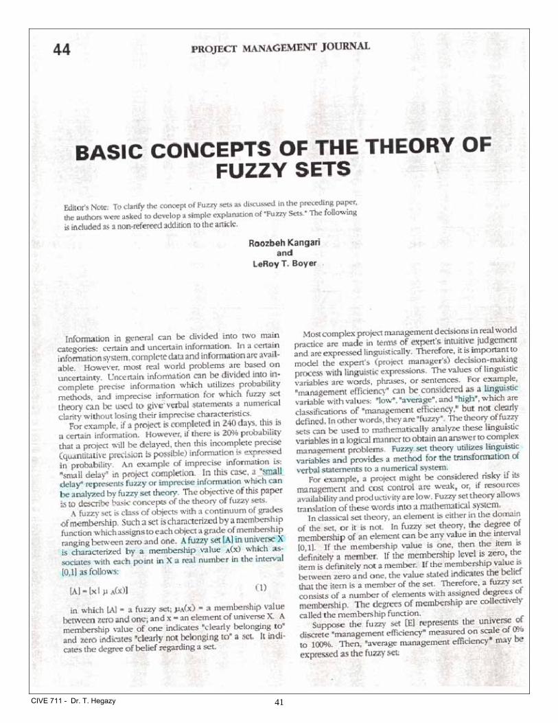
Fuzzy Sets & Fuzzy Logic 1965 Lotfi Zadeh – Fuzzy Sets (Loose Boundaries) i.e., everything is a matter of degree not True/False.

14 70 13 18 55 65 100 Other Shapes: Membership Functions: Height Young: X: ( 0, 13, 18);

µ: ( 1, 1 , 0) = Degree of membership

Set = X / µ = ( 0 / 1, 13 / 1 , 18 / 0 ) Middle: ( ) Old: ( )

Operations of Fuzzy Sets: AND OR NOT Example….Paper

100% = 1

Young Middle

100% = 1

Young Middle Old

1

0

Karate Baseball Volleyball

Young Middle Old

X

1

0

µ

13 18 55 65 100


1973 Fuzzy Logic (Linguistic variables):

Fuzzy Logic = Precisation of approximate reasoning.

- Car driving; Understanding language

- In Engineering, it is better to be approximately right than precisely wrong. Does it make sense to say that our project

will cost from $780,412.6 to $816,764.9?

- Many practical applications on machines and systems involving linguistic variables

- Natural language applications + Better web search engines based on Perception.

- In Google, How many horses got Ph.D. from the UW?

- What is the distance between the largest city in Spain and the largest city in France?

- Fuzzy Logic process: Fuzzification – IF-THEN rules – Defuzzification

- Example on Fuzzy Logic: Layout of Temporary Facilities

Code Facility Name A (M2) Type

11 8 9 3 10 6 12 5 1 7 2 4

Machine Room Parking Lot Tank Information and Guard Long Term Laydown Yard Cement Warehouse Scaffold Storage Yard Rebar Fab/Storage Yard Offices Testing Laboratory First Aid Toilet on Site

60 60 40 20 400 320 220 60 40 40 20 20

Fixed Fixed Fixed Fixed

Normal Normal Normal Normal Normal Normal Normal Normal

Men are mortal Joe is a man Then, Joe is Mortal

Most Sweeds are tall Joe is Sweed Then, Joe is likely to be tall


Fuzzy Decision Rules

Rule no. Work Flow

Safety/Environmental Concerns User's Preference Closeness

Rating

1 2 3 4 5 6 7 8 9 10 11 12 13 14 15 16 17 18 19 20 21 22 23 24 25 26 27

Low (L) Low (L) Low (L) Low (L) Low (L) Low (L) Low (L) Low (L) Low (L) Medium (M) Medium (M) Medium (M) Medium (M) Medium (M) Medium (M) Medium (M) Medium (M) Medium (M) High (H) High (H) High (H) High (H) High (H) High (H) High (H) High (H) High (H)

Low (L) Low (L) Low (L) Medium (M) Medium (M) Medium (M) High (H) High (H) High (H) Low (L) Low (L) Low (L) Medium (M) Medium (M) Medium (M) High (H) High (H) High (H) Low (L) Low (L) Low (L) Medium (M) Medium (M) Medium (M) High (H) High (H) High (H)

Low (L) Medium (M) High (H) Low (L) Medium (M) High (H) Low (L) Medium (M) High (H) Low (L) Medium (M) High (H) Low (L) Medium (M) High (H) Low (L) Medium (M) High (H) Low (L) Medium (M) High (H) Low (L) Medium (M) High (H) Low (L) Medium(M) High (H)

Ordinary (O) Important (I) Especially Important (E) Unimportant (U) Ordinary (O) Important (I) Undesirable (X) Unimportant (U) Ordinary (O) Important (I) Especially Important (E) Absolutely Important (A) Ordinary (O) Important (I) Especially Important (E) Unimportant (U) Ordinary (O) Important (I) Especially Important (E) Absolutely Important (A) Absolutely Important (A) Important (I) Especially Important (E) Absolutely Important (A) Ordinary (O) Important (I) Especially Important (E)

C.O.G = Σ (µ.x) / Σ µ


Hybrid Applications:


Infrastructure Asset Management While the civil infrastructure is the foundation for economic growth, a large percentage of its assets are rapidly deteriorating due to age, aggressive environment, and insufficient capacity for population growth. In 2003, the American Society of Civil Engineers released a report card on the infrastructures in the USA that gave failing grades to many infrastructure systems, and identified the need for $1.6 trillion (US) to bring the assets to acceptable condition (ASCE 2003). Similarly, the environmental, social, and transportation infrastructure systems in Canada require huge investments that amount to approximately $10 billion (US) annually for 10 years (Federation of Canadian Municipalities 1999). Since the environmental, social, and transportation sectors represent about 25% of the Canadian infrastructure expenditures (Figure1, Statistics Canada 1995), it can be assumed that the infrastructure system as whole requires an investment of about $40 billion per year for ten years. Despite of this large need, the Infrastructure Canada Program allocated only $2 billion (US) for the year 2000 to all infrastructure sectors (Federation of Canadian Municipalities 2001), thus covering only about 5% of the need. With the non-residential buildings being largest sector of the infrastructure (approximately 40%), such sector is expected to suffer the largest shortfall in expenditures on rehabilitation and repair.

Average yearly expenditures by type of infrastructure

Important Questions:

- What assets do you own? - What is it worth of each asset? - What is its current condition of asset components? - What is the remaining service life of the asset? - What is the predicted condition in the future? - What do you fix first? - How do you fix it? - What is the condition after the repair? - How will you execute the many repairs?

Important references: Please download from the course web page.

a) USA b) Canada

Marine 1%

Non- Residential

Buildings 40%

Other 5%

Oil and Gas 21%

Communication 4%

Electric 10%

Transportatin14%

Water 2% Sewage 3%

Transportation 14%

Non- Residential

Buildings 63%

Other 8%

Oil and Gas 2%Communication 4%

Water 2% Sewage 3%

Electric 4%


- Problems with CPM & PDM - Resource-Driven Scheduling - Crew Work Continuity - Learning Phenomenon

Integrated CPM & LOB Calculations:

New Representation:

Crew Synchronization Calculations:

Crews (C) = (D) x (R)

Calculating a Desired

Progress Rate (R):

Scheduling Repetitive & Linear Projects

Time

n

.

.

.

2

1

Uni

ts

R


Example:

For this small project, the work hours and the number of workers for each activity are shown. if you are to construct these tasks for 5 houses in 21 days, calculate the number of crews that need in each activity. Draw the schedule and show when each crew enters and leaves the site;

Step 1: CPM Calculation

Step 2: LOB Calculations Deadline TL = 21; T1 = ___ ; n = 5

Activity

Duration (D)

Total Float (TF)

Desired Rate (R) (n-1) / (TL-T1+TF)

Min. Crews

(C) = D x R

Actual Crews

(Ca)

Actual Rate

(Ra) = Ca / D A

B

C

D

E

F

Step 3: Draw the Chart

A. Excavation 48 hrs, 3 W

C. Footing 1 64 hrs, 2 W

E. Wall 1 72 hrs, 3 W

F. Wall 2 72 hrs, 3 W

B. Sanit. Main48 hrs, 3 W

D. Footing 2 64 hrs, 2 W

1 2 3 4 5 6 7 8 9 10 11 12 13 14 15 16 17 18 19 20 21 22 23 24 25

1 2 3 4 5 6 7 8 9 10 11 12 13 14 15 16 17 18 19 20 21 22 23 24 25

Assume:

- Same no. of Crews - Activity A in unit 2 has double the duration - Unit 4 does not need excavation.

Draw the critical path


More Advanced Linear scheduling Model Flexible features for scheduling the activities include: color-coded or pattern-coded crews; varying quantities; productivity impact; crew interruption time; crew staggering; crew work sequence; and activities’ progress speeds (slopes of lines). It is noted that the schedule is efficiently arranged with crew work continuity maintained. Also, overlapping is avoided by simply showing the activities of each path in the work network separately. In addition:

1. Activities are not necessarily repeated at all sections.

2. Activities can proceed in an ascending or descending flow. This provides work flow flexibility and

provides for a way to fast-track projects;

3. Each activity has up to 3 methods of construction (e.g., normal work, overtime, or subcontractor) with

associated time, cost, and crew constraints. The model can then be used to select the proper

combination of methods that meet the deadline, cost, and crew constraints;

4. Activities can have non-standard durations and costs at selected sections;

5. Work interruption (layoff period) can be specified by the user at any unit of any activity; and

6. Conditional methods of construction can be specified by the user.

Top crew works from

station 9 to 5, while bottom crew works

from station 1 to 4.

UN

IT N

O.

TIME1

4

5

3

6

2

9

8

7

Crew 3

Crew 2

No work at station 8.

Small quantity at Station 4.

Low productivity at Station 2 (Large

duration).Crew 1

Crew 2

Crew 1

Crew 1

Crew 3

Work proceeds from station 3 to

8 only, with interruption at

station 5.

Work proceeds forward from

station 3 to 8 only.

Activity A Activity B Activity C Activity D


2 PARALLEL CREWS

3 Staggered

Inde

x to

Site

Num

ber

TIME1

4

5

3

6

2

9

8

7

Crew 1

Crew 2

Out-Tasked

Crew 1

Crew 2

Crew 1

Crew 2

Crew 1

Crew 2

Crew 3

Crew 1

Crew 2

Crew 3

Crew 1

Crew 1

Crew 2

Crew 3

Crew 1

Crew 2

Crew 2

Crew 3

Outsourced site

Outsourced site

Available crew is assigned

Infrastructure Networks with Distributed Sites: A Bigger Challenge Buildings, Hispitals, Schools, Highway Spots, Bridges

Delivery approaches for MR&R programs

Effect of Site order

Scheduling of crews along multiple sites


Baseline

Current schedule

Project Control

Organize site? Recording of site events? Work Status? Comparing Planned versus Actual? Progress Payments? Managing Changes? Updating? Corrective Actions? Delay Resposibility? Forecasting/

Time Extension? Cost compensation? Productivity Assessment? Saving All As-Built Details? Lessons Learned? a) Organized Site = Safety + Productivity + Good Circulation + Cost & Time Savings

(1) identifying necessary facilities and determining their appropriate sizes; (2) determining the inter-relationships among the facilities on the site; and (3) optimizing the placement of the facilities on the site plan.

b) Recording Site events Calculate activity % complete, Camcorders, Time-Lapse Camera, Minutes, Project Web Site

Calculating activity % complete: pages 291& 292

Calculating the overall project % complete: page 293 c) Using Software

How to show Delays? Slow versus Fast? Reasons for work stops?

Can we readily decide which party is responsible for the two days delay beyond the deadline?

Work Stop Acceleration Slow-down

• Reason? • Owner Directed?• Contractor own? • Document?

Activity % Complete

% complete % complete actual planned ⟨

% Actual complete = 0 ⟩

% complete % complete actual planned

Owner (O)

Contractor (C)

Neither (N)

Responsibility and reason

• Reason? • Document?


d) Techniques for Performance Evaluation

1. S-Curve Envelope:

Early versus Late bar chart

2. Earned-Value Analysis:

Schedule Performance Index (SPI) = BCWP BCWS

Cost Performance Index (CPI) = BCWP ACWP

BCWS Budget Price

ACWP Actual Cost

BCWP (EV) Time

$

Direct + Indirect Costs

Time

Contractor’s cost Control

3 piles = $ 7 piles = $ 3 piles = $ Progress Date

Budget for 1 pile = $10,000; Actual cost of 1 pile = $40,000 On Progress Date:

Work Scheduled = 7 Piles; Work Performed= 3 Piles

- Time variance? - Estimate at completion?


e) Agenda for Success:

- Get Good Designers: Beware of Bargain Shopping; - Watch Low Bids Carefully: Work at Cost Spells Trouble; - Fail to Plan and you Plan to Fail; - Keep the Work Site Organized; - Monitor the Gaps; - No Pay Causes Delay; - Time = Money; - Communication; and Documentation.

f) New Concept For Project Control (Critical Chain):

- Estimate with safety removed (50% chance); - Incentive for early finish; - Focus on predecessors’ finish; - Project buffer (50%); - Simple monitoring of buffer penetration; - Earned-Value for cost analysis.

CPI

1.1

1.2

1.0

1.1 1.2 0.9 0.8

0.9

0.8

SPI

Over Cost, Ahead of Schedule

Under Cost, Ahead of Schedule

Under Cost, Behind Schedule

Over Cost, Behind Schedule

Start