cfx12 03 physics1
TRANSCRIPT
3-1ANSYS, Inc. Proprietary© 2009 ANSYS, Inc. All rights reserved.
April 28, 2009Inventory #002598
Chapter 3
Domains andBoundary Conditions
Introduction to CFX
Boundary Conditions
3-2ANSYS, Inc. Proprietary© 2009 ANSYS, Inc. All rights reserved.
April 28, 2009Inventory #002598
Training ManualDomains
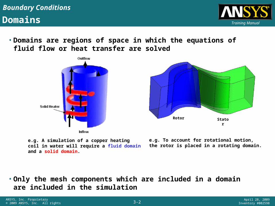
• Domains are regions of space in which the equations of fluid flow or heat transfer are solved
• Only the mesh components which are included in a domain are included in the simulation
e.g. A simulation of a copper heating coil in water will require a fluid domain and a solid domain.
e.g. To account for rotational motion, the rotor is placed in a rotating domain.
Rotor Stator

Boundary Conditions
3-3ANSYS, Inc. Proprietary© 2009 ANSYS, Inc. All rights reserved.
April 28, 2009Inventory #002598
Training ManualHow to Create a Domain (as shown earlier)
Define Domain Properties– Right-click on the domain and pick Edit– Or right-click on Flow Analysis 1 to insert a new domain
When editing an item a new tab panel opens containing the properties. You can switch between open tabs.
Sub-tabs contain various different properties
Complete the required fields on each sub-tab to define the domain
Optional fields are activated by enabling a check box
Boundary Conditions
3-4ANSYS, Inc. Proprietary© 2009 ANSYS, Inc. All rights reserved.
April 28, 2009Inventory #002598
Training ManualDomain Creation
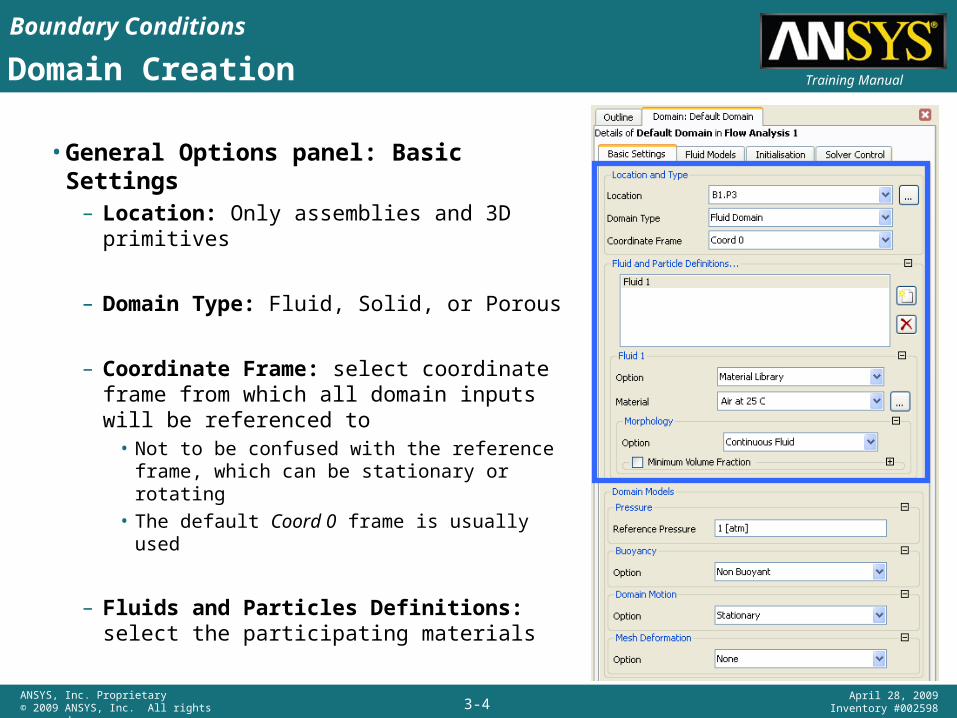
• General Options panel: Basic Settings– Location: Only assemblies and 3D
primitives
– Domain Type: Fluid, Solid, or Porous
– Coordinate Frame: select coordinate frame from which all domain inputs will be referenced to
• Not to be confused with the reference frame, which can be stationary or rotating
• The default Coord 0 frame is usually used
– Fluids and Particles Definitions: select the participating materials

Boundary Conditions
3-5ANSYS, Inc. Proprietary© 2009 ANSYS, Inc. All rights reserved.
April 28, 2009Inventory #002598
Training Manual
Ex. 2: Preference= 100,000 Pa
Domain Creation – Reference Pressure• General Options panel: Domain Models
– Reference Pressure • Represents the absolute pressure datum from
which all relative pressures are measured
Pabs = Preference + Prelative
• Pressures specified at boundary and initial conditions are relative to the Reference Pressure
• Used to avoid problems with round-off errors which occur when the local pressure differences in a fluid are small compared to the absolute pressure level
PressurePressure
Ex. 1: Preference= 0 Pa
Pref
Prel,max=100,001 Pa
Prel,min=99,999 Pa
Prel,max=1 Pa
Prel,min=-1 Pa
Pref
Boundary Conditions
3-6ANSYS, Inc. Proprietary© 2009 ANSYS, Inc. All rights reserved.
April 28, 2009Inventory #002598
Training ManualDomain Creation - Buoyancy
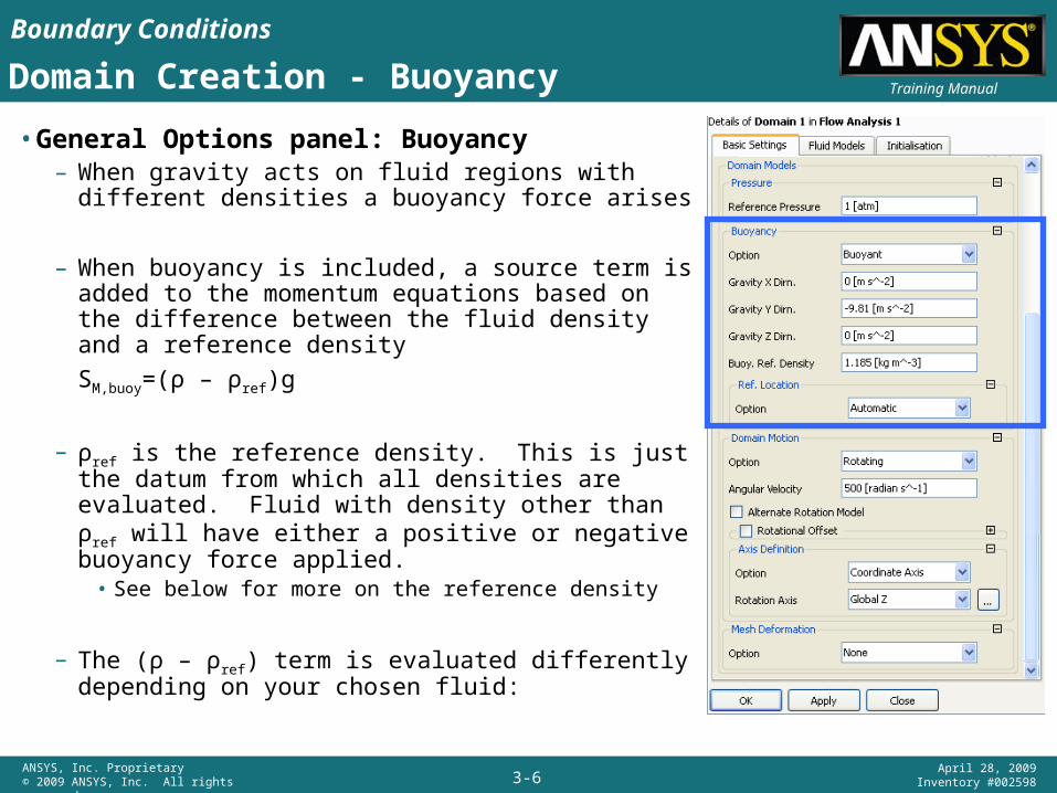
• General Options panel: Buoyancy– When gravity acts on fluid regions with different
densities a buoyancy force arises
– When buoyancy is included, a source term is added to the momentum equations based on the difference between the fluid density and a reference density
SM,buoy=(ρ – ρref)g
– ρref is the reference density. This is just the datum from which all densities are evaluated. Fluid with density other than ρref will have either a positive or negative buoyancy force applied.
• See below for more on the reference density
– The (ρ – ρref) term is evaluated differently depending on your chosen fluid:
Boundary Conditions
3-7ANSYS, Inc. Proprietary© 2009 ANSYS, Inc. All rights reserved.
April 28, 2009Inventory #002598
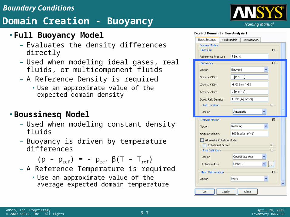
Training ManualDomain Creation - Buoyancy• Full Buoyancy Model
– Evaluates the density differences directly– Used when modeling ideal gases, real fluids, or
multicomponent fluids– A Reference Density is required
• Use an approximate value of the expected domain density
• Boussinesq Model– Used when modeling constant density fluids– Buoyancy is driven by temperature differences
(ρ – ρref) = - ρref β(T – Tref)– A Reference Temperature is required
• Use an approximate value of the average expected domain temperature
Boundary Conditions
3-8ANSYS, Inc. Proprietary© 2009 ANSYS, Inc. All rights reserved.
April 28, 2009Inventory #002598
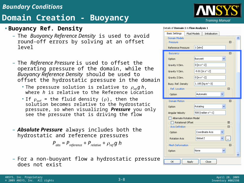
Training ManualDomain Creation - Buoyancy• Buoyancy Ref. Density
– The Buoyancy Reference Density is used to avoid round-off errors by solving at an offset level
– The Reference Pressure is used to offset the operating pressure of the domain, while the Buoyancy Reference Density should be used to offset the hydrostatic pressure in the domain
• The pressure solution is relative to ref g h, where h is relative to the Reference Location
• If ref = the fluid density (), then the solution becomes relative to the hydrostatic pressure, so when visualizing Pressure you only see the pressure that is driving the flow
– Absolute Pressure always includes both the hydrostatic and reference pressures
Pabs = Preference + Prelative + ref g h
– For a non-buoyant flow a hydrostatic pressure does not exist
Boundary Conditions
3-9ANSYS, Inc. Proprietary© 2009 ANSYS, Inc. All rights reserved.
April 28, 2009Inventory #002598
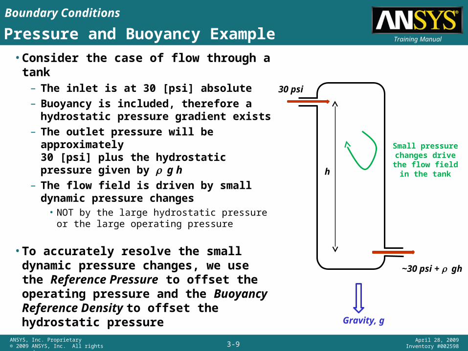
Training ManualPressure and Buoyancy Example
• Consider the case of flow through a tank– The inlet is at 30 [psi] absolute– Buoyancy is included, therefore a
hydrostatic pressure gradient exists– The outlet pressure will be approximately
30 [psi] plus the hydrostatic pressure given by g h
– The flow field is driven by small dynamic pressure changes
• NOT by the large hydrostatic pressure or the large operating pressure
• To accurately resolve the small dynamic pressure changes, we use the Reference Pressure to offset the operating pressure and the Buoyancy Reference Density to offset the hydrostatic pressure
30 psi
h
~30 psi + gh
Gravity, g
Small pressure changes drive the
flow field in the tank
Boundary Conditions
3-10ANSYS, Inc. Proprietary© 2009 ANSYS, Inc. All rights reserved.
April 28, 2009Inventory #002598
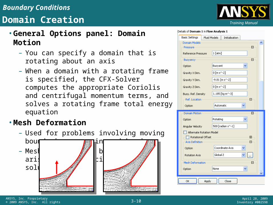
Training ManualDomain Creation• General Options panel: Domain Motion
– You can specify a domain that is rotating about an axis
– When a domain with a rotating frame is specified, the CFX-Solver computes the appropriate Coriolis and centrifugal momentum terms, and solves a rotating frame total energy equation
• Mesh Deformation– Used for problems involving moving boundaries
or moving subdomains– Mesh motion could be imposed or arise as an
implicit part of the solution
Boundary Conditions
3-11ANSYS, Inc. Proprietary© 2009 ANSYS, Inc. All rights reserved.
April 28, 2009Inventory #002598
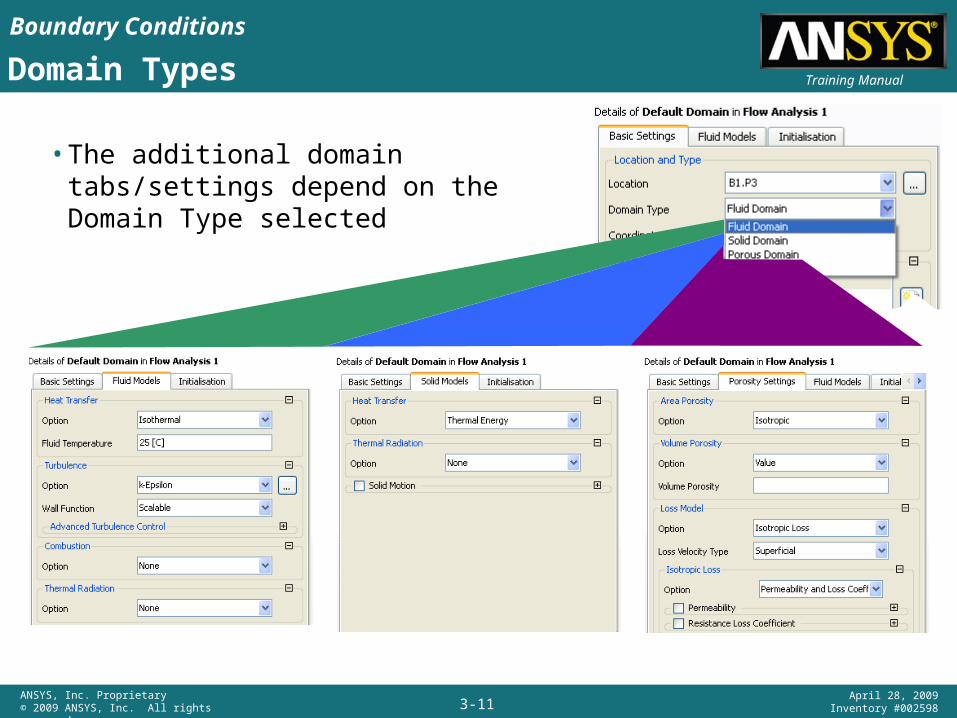
Training ManualDomain Types
• The additional domain tabs/settings depend on the Domain Type selected
Boundary Conditions
3-12ANSYS, Inc. Proprietary© 2009 ANSYS, Inc. All rights reserved.
April 28, 2009Inventory #002598
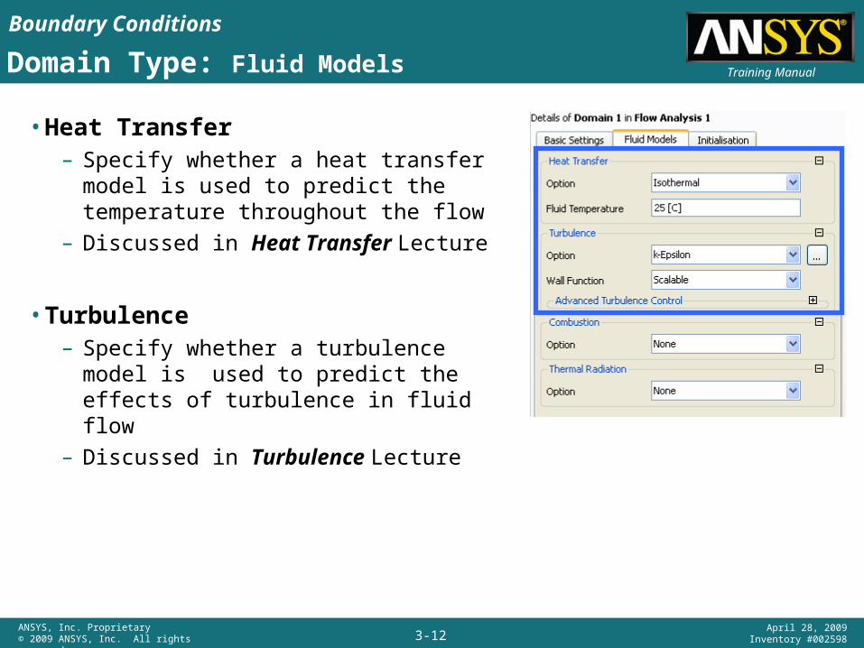
Training ManualDomain Type: Fluid Models
• Heat Transfer– Specify whether a heat transfer model is
used to predict the temperature throughout the flow
– Discussed in Heat Transfer Lecture
• Turbulence – Specify whether a turbulence model is
used to predict the effects of turbulence in fluid flow
– Discussed in Turbulence Lecture

Boundary Conditions
3-13ANSYS, Inc. Proprietary© 2009 ANSYS, Inc. All rights reserved.
April 28, 2009Inventory #002598
Training ManualDomain Type: Fluid Models
Reaction or Combustion Models– CFX includes combustion models to allow the
simulation of flows in which combustion reactions occur
– Available only if Option = Material Definition on the Basic Settings tab
– Not covered in detail in this course
Boundary Conditions
3-14ANSYS, Inc. Proprietary© 2009 ANSYS, Inc. All rights reserved.
April 28, 2009Inventory #002598
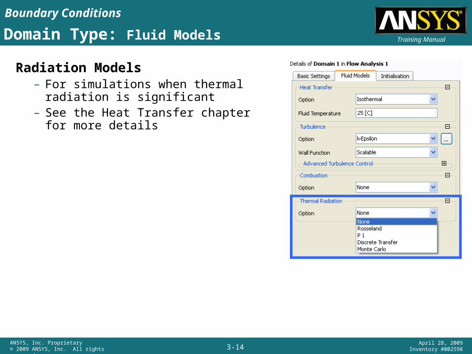
Training ManualDomain Type: Fluid Models
Radiation Models– For simulations when thermal radiation is
significant– See the Heat Transfer chapter for more
details
Boundary Conditions
3-15ANSYS, Inc. Proprietary© 2009 ANSYS, Inc. All rights reserved.
April 28, 2009Inventory #002598
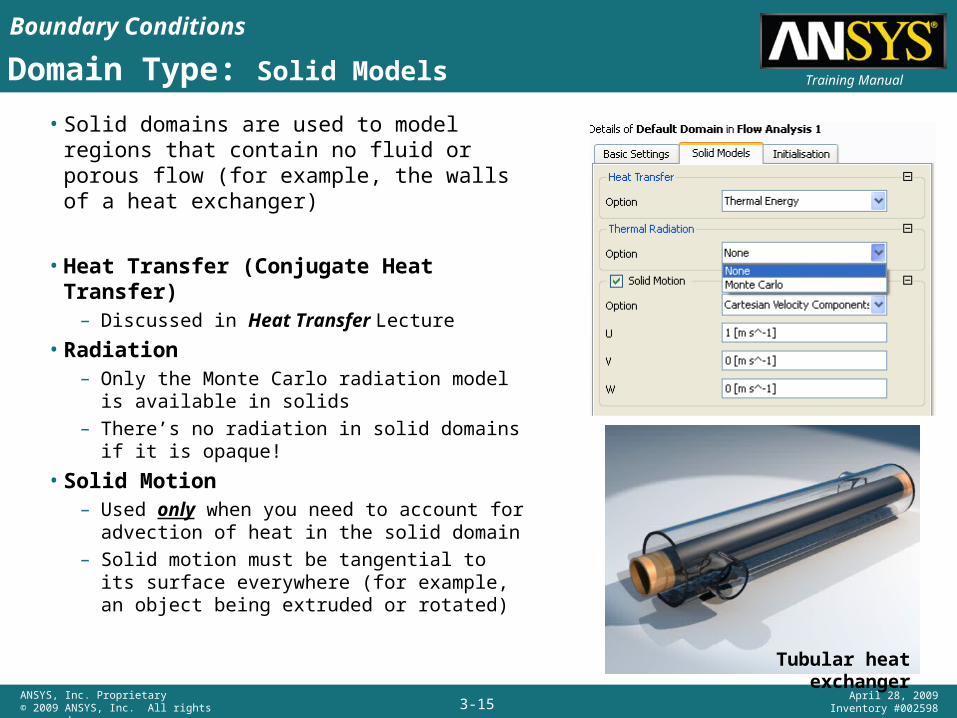
Training ManualDomain Type: Solid Models
• Solid domains are used to model regions that contain no fluid or porous flow (for example, the walls of a heat exchanger)
• Heat Transfer (Conjugate Heat Transfer)– Discussed in Heat Transfer Lecture
• Radiation – Only the Monte Carlo radiation model is
available in solids– There’s no radiation in solid domains if it is
opaque!
• Solid Motion– Used only when you need to account for
advection of heat in the solid domain– Solid motion must be tangential to its
surface everywhere (for example, an object being extruded or rotated)
Tubular heat exchanger

Boundary Conditions
3-16ANSYS, Inc. Proprietary© 2009 ANSYS, Inc. All rights reserved.
April 28, 2009Inventory #002598
Training Manual
Images Courtesy of Babcock and Wilcox, USA
Domain Type: Porous Domains
• Used to model flows where the geometry is too complex to resolve with a grid
• Instead of including the geometric details, their effects are accounted for numerically

Boundary Conditions
3-17ANSYS, Inc. Proprietary© 2009 ANSYS, Inc. All rights reserved.
April 28, 2009Inventory #002598
Training ManualDomain Type: Porous Domains
• Area Porosity– The area porosity (the fraction of physical
area that is available for the flow to go through) is assumed isotropic
• Volume Porosity– The local ratio of the volume of fluid to the
total physical volume (can vary spatially)– By default, the velocity solved by the code
is the superficial fluid velocity. In a porous region, the true fluid velocity of the fluid will be larger because of the flow volume reduction Superficial Velocity = Volume Porosity * True Velocity This setting should be
consistent with the velocity used when
the Loss Coefficients (next slide) were
calculated
Boundary Conditions
3-18ANSYS, Inc. Proprietary© 2009 ANSYS, Inc. All rights reserved.
April 28, 2009Inventory #002598
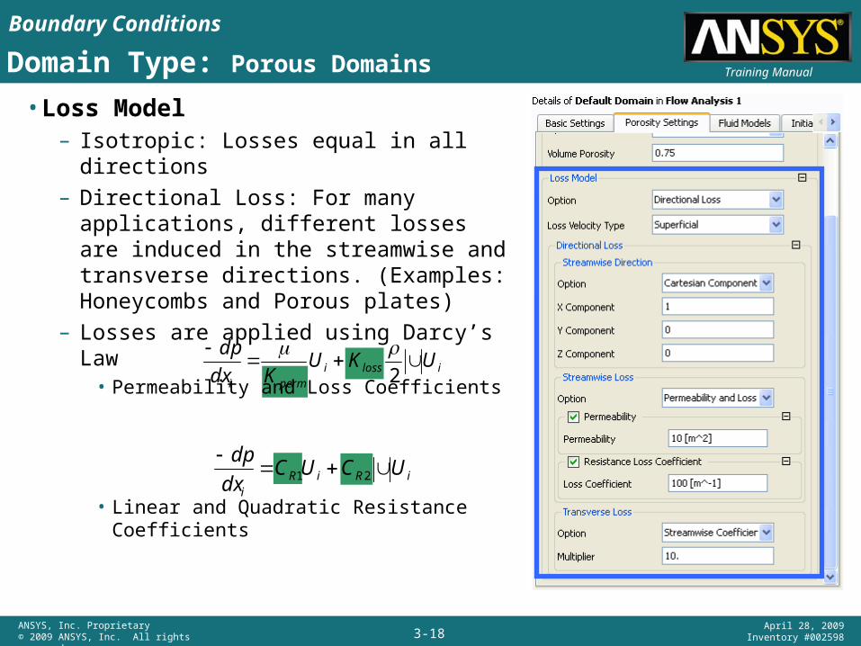
Training ManualDomain Type: Porous Domains
• Loss Model– Isotropic: Losses equal in all directions– Directional Loss: For many applications,
different losses are induced in the streamwise and transverse directions. (Examples: Honeycombs and Porous plates)
– Losses are applied using Darcy’s Law• Permeability and Loss Coefficients
• Linear and Quadratic Resistance Coefficients
ilossipermi
UKUKdx
dp
2
ilossipermi
UKUKdx
dp
2
iRiRi
UCUCdx
dp21
Boundary Conditions
3-19ANSYS, Inc. Proprietary© 2009 ANSYS, Inc. All rights reserved.
April 28, 2009Inventory #002598
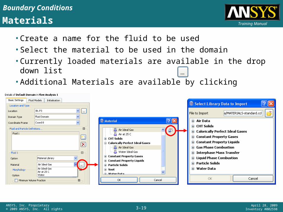
Training ManualMaterials
• Create a name for the fluid to be used• Select the material to be used in the domain• Currently loaded materials are available in the drop down list• Additional Materials are available by clicking
Boundary Conditions
3-20ANSYS, Inc. Proprietary© 2009 ANSYS, Inc. All rights reserved.
April 28, 2009Inventory #002598
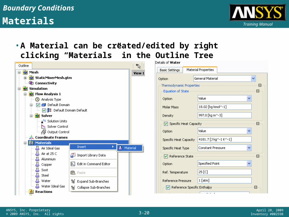
Training ManualMaterials
• A Material can be created/edited by right clicking “Materials” in the Outline Tree
Boundary Conditions
3-21ANSYS, Inc. Proprietary© 2009 ANSYS, Inc. All rights reserved.
April 28, 2009Inventory #002598
Training ManualMulticomponent/Multiphase Flow
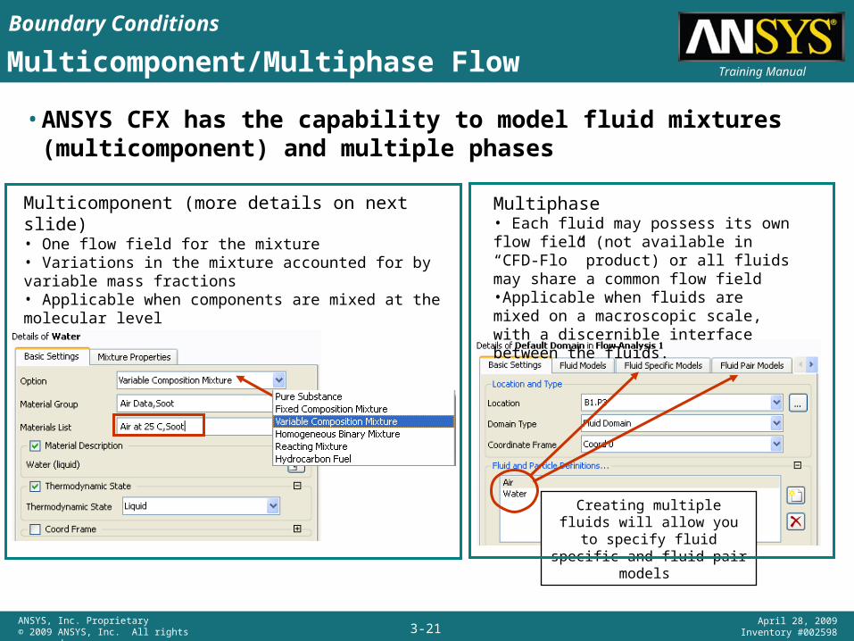
• ANSYS CFX has the capability to model fluid mixtures (multicomponent) and multiple phases
Multicomponent (more details on next slide)• One flow field for the mixture• Variations in the mixture accounted for by variable mass fractions • Applicable when components are mixed at the molecular level
Multiphase• Each fluid may possess its own flow field (not available in “CFD-Flo” product) or all fluids may share a common flow field•Applicable when fluids are mixed on a macroscopic scale, with a discernible interface between the fluids.
Creating multiple fluids will allow you to specify fluid
specific and fluid pair models
Boundary Conditions
3-22ANSYS, Inc. Proprietary© 2009 ANSYS, Inc. All rights reserved.
April 28, 2009Inventory #002598
Training ManualMulticomponent Flow
• Each component fluid may have a distinct set of physical properties
• The ANSYS CFX-Solver will calculate appropriate average values of the properties for each control volume in the flow domain, for use in calculating the fluid flow
• These average values will depend both on component property values and on the proportion of each component present in the control volume
• In multicomponent flow, the various components of a fluid share the same mean velocity, pressure and temperature fields, and mass transfer takes place by convection and diffusion
Boundary Conditions
3-23ANSYS, Inc. Proprietary© 2009 ANSYS, Inc. All rights reserved.
April 28, 2009Inventory #002598
Training ManualCompressible Flow Modelling
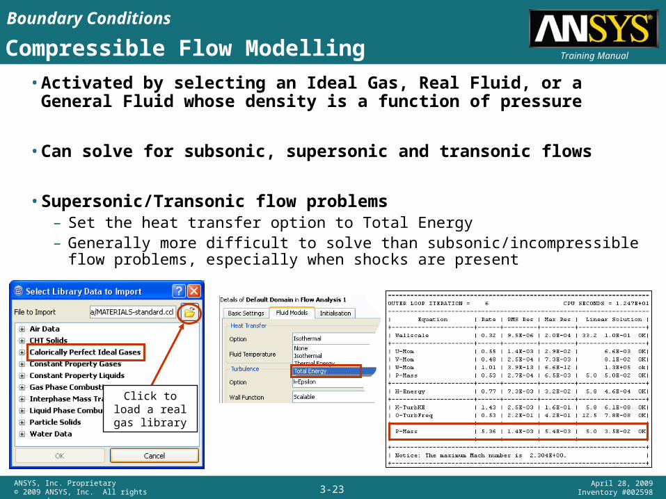
• Activated by selecting an Ideal Gas, Real Fluid, or a General Fluid whose density is a function of pressure
• Can solve for subsonic, supersonic and transonic flows
• Supersonic/Transonic flow problems – Set the heat transfer option to Total Energy– Generally more difficult to solve than subsonic/incompressible flow problems,
especially when shocks are present
Click to load a real gas library

3-24ANSYS, Inc. Proprietary© 2009 ANSYS, Inc. All rights reserved.
April 28, 2009Inventory #002598
Boundary Conditions
Boundary Conditions
3-25ANSYS, Inc. Proprietary© 2009 ANSYS, Inc. All rights reserved.
April 28, 2009Inventory #002598
Training ManualDefining Boundary Conditions
• You must specify information on the dependent (flow) variables at the domain boundaries
– Specify fluxes of mass, momentum, energy, etc. into the domain.
• Defining boundary conditions involves:– Identifying the location of the boundaries (e.g., inlets, walls, symmetry)– Supplying information at the boundaries
• The data required at a boundary depends upon the boundary condition type and the physical models employed
• You must be aware of types of the boundary condition available and locate the boundaries where the flow variables have known values or can be reasonably approximated
– Poorly defined boundary conditions can have a significant impact on your solution
Boundary Conditions
3-26ANSYS, Inc. Proprietary© 2009 ANSYS, Inc. All rights reserved.
April 28, 2009Inventory #002598
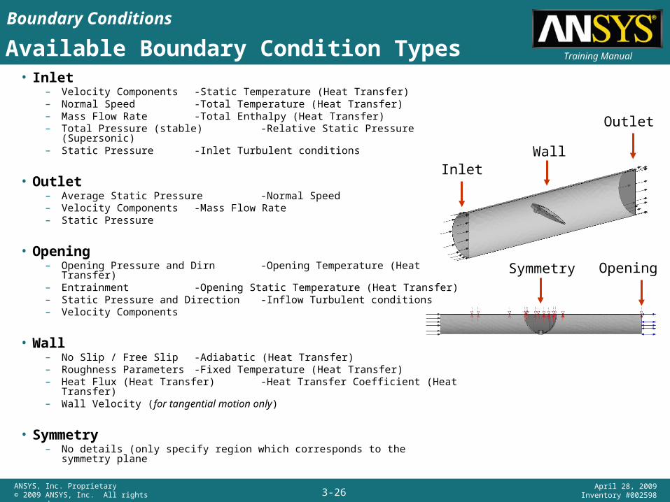
Training ManualAvailable Boundary Condition Types• Inlet
– Velocity Components -Static Temperature (Heat Transfer)– Normal Speed -Total Temperature (Heat Transfer)– Mass Flow Rate -Total Enthalpy (Heat Transfer)– Total Pressure (stable) -Relative Static Pressure (Supersonic)– Static Pressure -Inlet Turbulent conditions
• Outlet– Average Static Pressure -Normal Speed– Velocity Components -Mass Flow Rate– Static Pressure
• Opening– Opening Pressure and Dirn -Opening Temperature (Heat Transfer)– Entrainment -Opening Static Temperature (Heat Transfer)– Static Pressure and Direction-Inflow Turbulent conditions– Velocity Components
• Wall– No Slip / Free Slip -Adiabatic (Heat Transfer)– Roughness Parameters -Fixed Temperature (Heat Transfer)– Heat Flux (Heat Transfer) -Heat Transfer Coefficient (Heat Transfer)– Wall Velocity (for tangential motion only)
• Symmetry– No details (only specify region which corresponds to the symmetry plane
Inlet
Opening
Outlet
Wall
Symmetry
Boundary Conditions
3-27ANSYS, Inc. Proprietary© 2009 ANSYS, Inc. All rights reserved.
April 28, 2009Inventory #002598
Training Manual
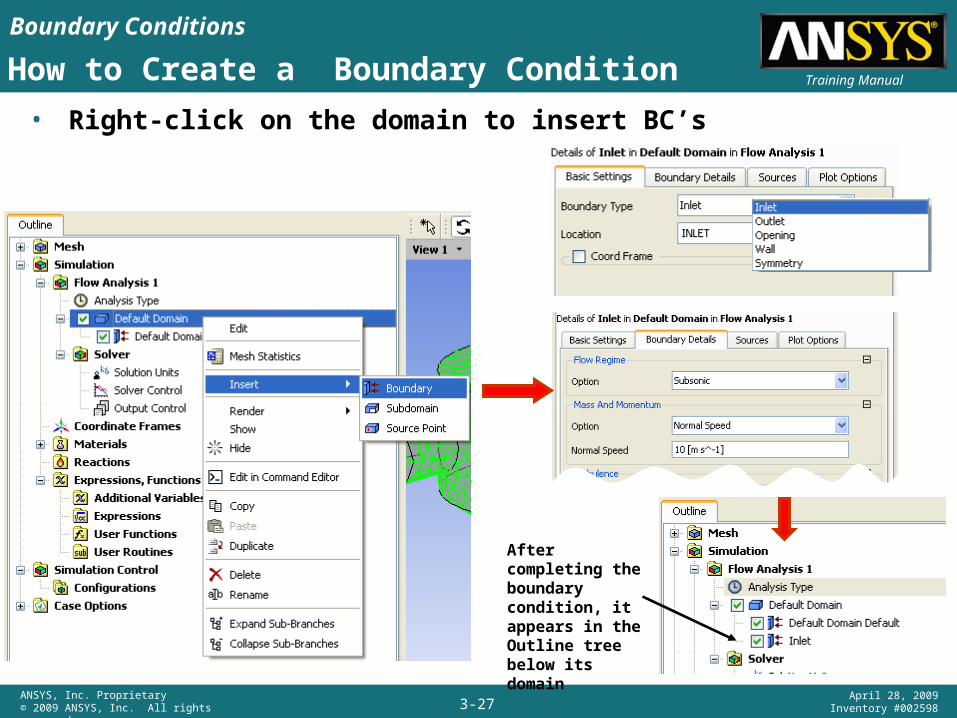
• Right-click on the domain to insert BC’s
How to Create a Boundary Condition
After completing the boundary condition, it appears in the Outline tree below its domain
Boundary Conditions
3-28ANSYS, Inc. Proprietary© 2009 ANSYS, Inc. All rights reserved.
April 28, 2009Inventory #002598
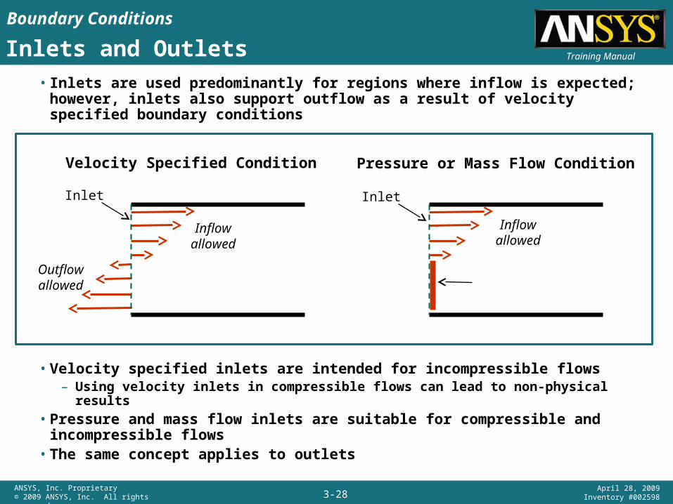
Training ManualInlets and Outlets
• Inlets are used predominantly for regions where inflow is expected; however, inlets also support outflow as a result of velocity specified boundary conditions
• Velocity specified inlets are intended for incompressible flows– Using velocity inlets in compressible flows can lead to non-physical results
• Pressure and mass flow inlets are suitable for compressible and incompressible flows
• The same concept applies to outlets
Velocity Specified Condition Pressure or Mass Flow Condition
Inlet Inlet
Inflow allowed
Inflowallowed
Outflowallowed
Boundary Conditions
3-29ANSYS, Inc. Proprietary© 2009 ANSYS, Inc. All rights reserved.
April 28, 2009Inventory #002598
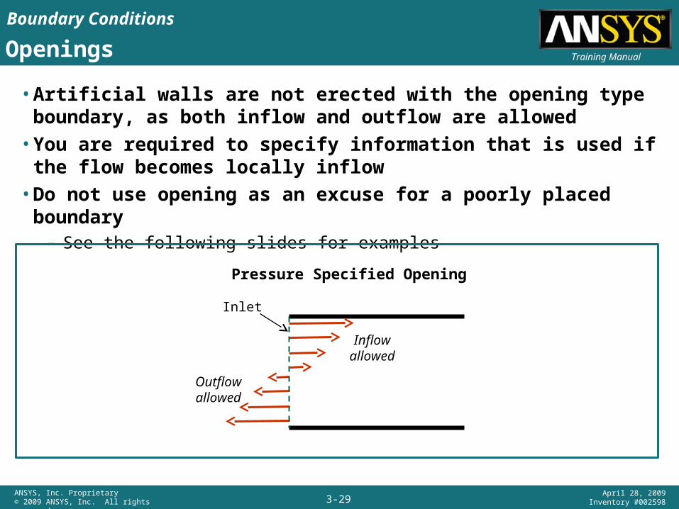
Training ManualOpenings
• Artificial walls are not erected with the opening type boundary, as both inflow and outflow are allowed
• You are required to specify information that is used if the flow becomes locally inflow
• Do not use opening as an excuse for a poorly placed boundary– See the following slides for examples
Pressure Specified Opening
Inlet
Inflow allowed
Outflowallowed

Boundary Conditions
3-30ANSYS, Inc. Proprietary© 2009 ANSYS, Inc. All rights reserved.
April 28, 2009Inventory #002598
Training ManualSymmetry
• Used to reduce computational effort in problem.
• No inputs are required.
• Flow field and geometry must be symmetric:– Zero normal velocity at symmetry plane– Zero normal gradients of all variables at symmetry plane– Must take care to correctly define symmetry boundary locations
• Can be used to model slip walls in viscous flow
symmetry planes
Boundary Conditions
3-31ANSYS, Inc. Proprietary© 2009 ANSYS, Inc. All rights reserved.
April 28, 2009Inventory #002598
Training Manual
Fuel
Air
Manifold box1Nozzle
1
23
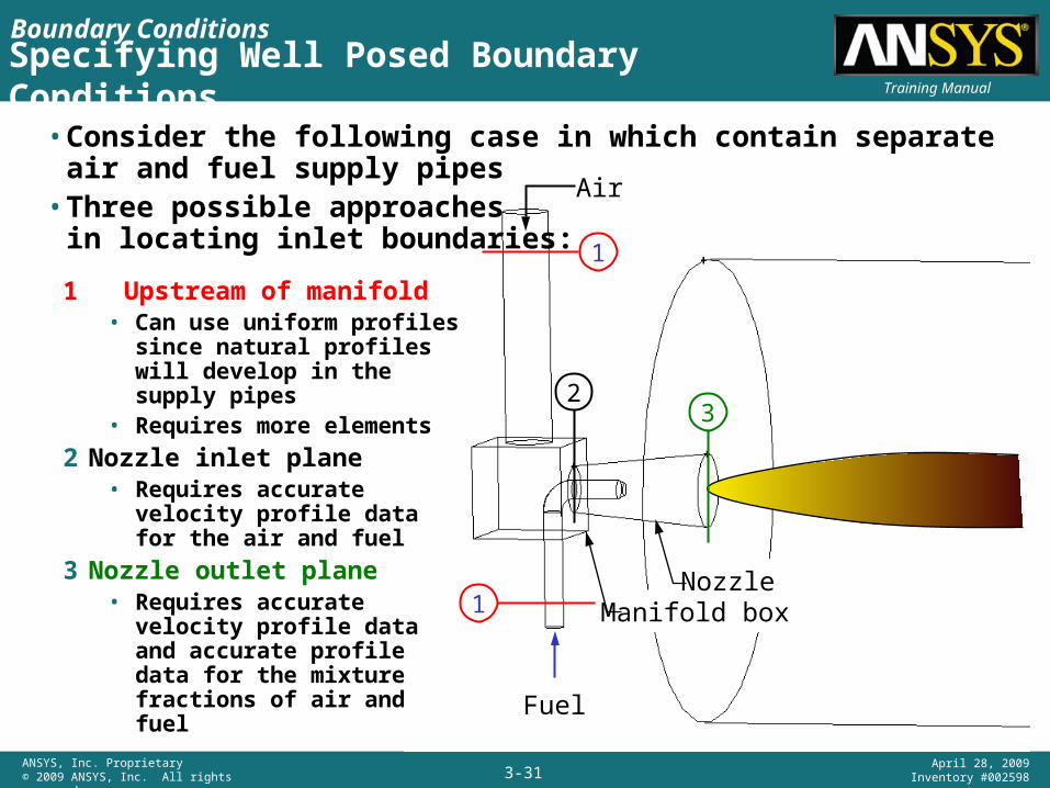
Specifying Well Posed Boundary Conditions
1 Upstream of manifold• Can use uniform profiles
since natural profiles will develop in the supply pipes
• Requires more elements
2 Nozzle inlet plane• Requires accurate velocity
profile data for the air and fuel
3 Nozzle outlet plane• Requires accurate velocity
profile data and accurate profile data for the mixture fractions of air and fuel
• Consider the following case in which contain separate air and fuel supply pipes
• Three possible approachesin locating inlet boundaries:
Boundary Conditions
3-32ANSYS, Inc. Proprietary© 2009 ANSYS, Inc. All rights reserved.
April 28, 2009Inventory #002598
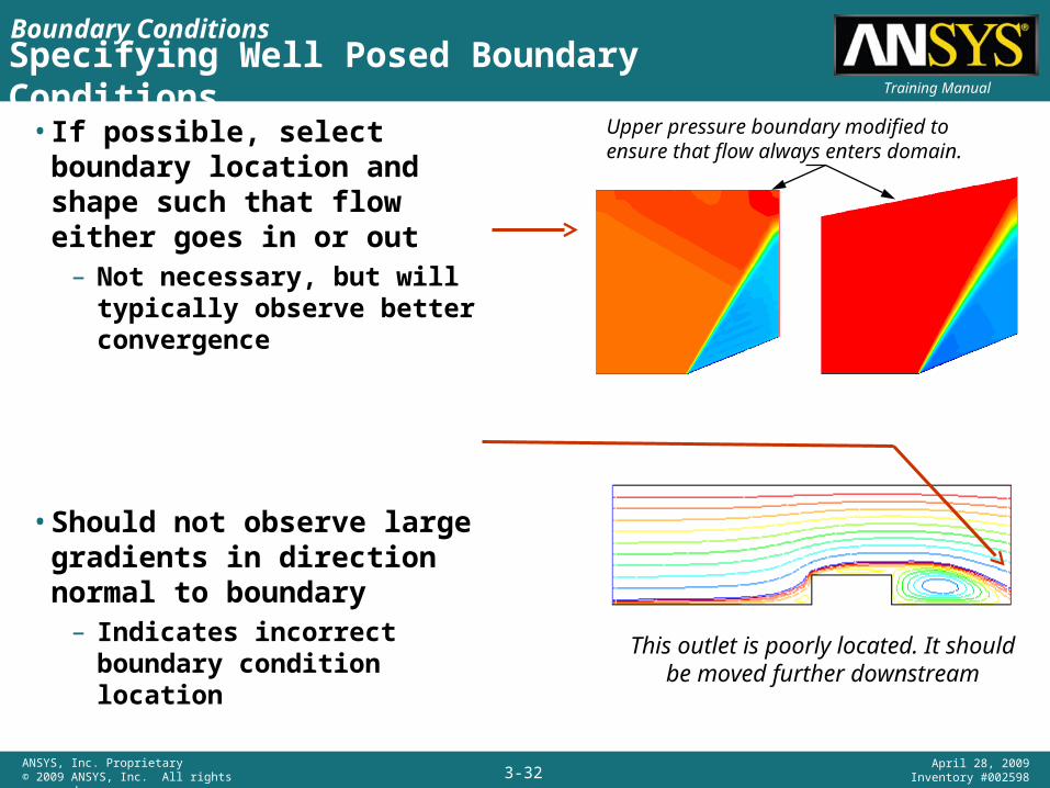
Training ManualSpecifying Well Posed Boundary Conditions
• If possible, select boundary location and shape such that flow either goes in or out
– Not necessary, but will typically observe better convergence
• Should not observe large gradients in direction normal to boundary
– Indicates incorrect boundary condition location
Upper pressure boundary modified to ensure that flow always enters domain.
This outlet is poorly located. It should be moved further downstream
Boundary Conditions
3-33ANSYS, Inc. Proprietary© 2009 ANSYS, Inc. All rights reserved.
April 28, 2009Inventory #002598
Training Manual
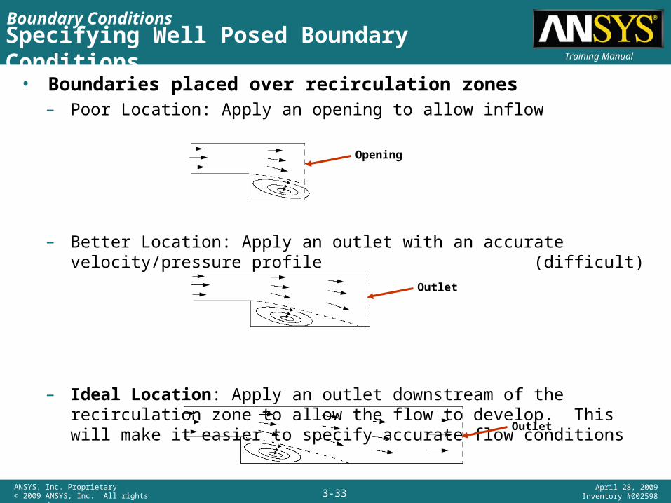
• Boundaries placed over recirculation zones– Poor Location: Apply an opening to allow inflow
– Better Location: Apply an outlet with an accurate velocity/pressure profile (difficult)
– Ideal Location: Apply an outlet downstream of the recirculation zone to allow the flow to develop. This will make it easier to specify accurate flow conditions
Specifying Well Posed Boundary Conditions
Opening
Outlet
Outlet
Boundary Conditions
3-34ANSYS, Inc. Proprietary© 2009 ANSYS, Inc. All rights reserved.
April 28, 2009Inventory #002598
Training Manual
• Turbulence at the Inlet– Nominal turbulence intensities range from 1% to 5% but will depend
on your specific application.
– The default turbulence intensity value of 0.037 (that is, 3.7%) is sufficient for nominal turbulence through a circular inlet, and is a good estimate in the absence of experimental data.
– For situations where turbulence is generated by wall friction, consider extending the domain upstream to allow the walls to generate turbulence and the flow to become developed
Specifying Well Posed Boundary Conditions
Boundary Conditions
3-35ANSYS, Inc. Proprietary© 2009 ANSYS, Inc. All rights reserved.
April 28, 2009Inventory #002598
Training Manual
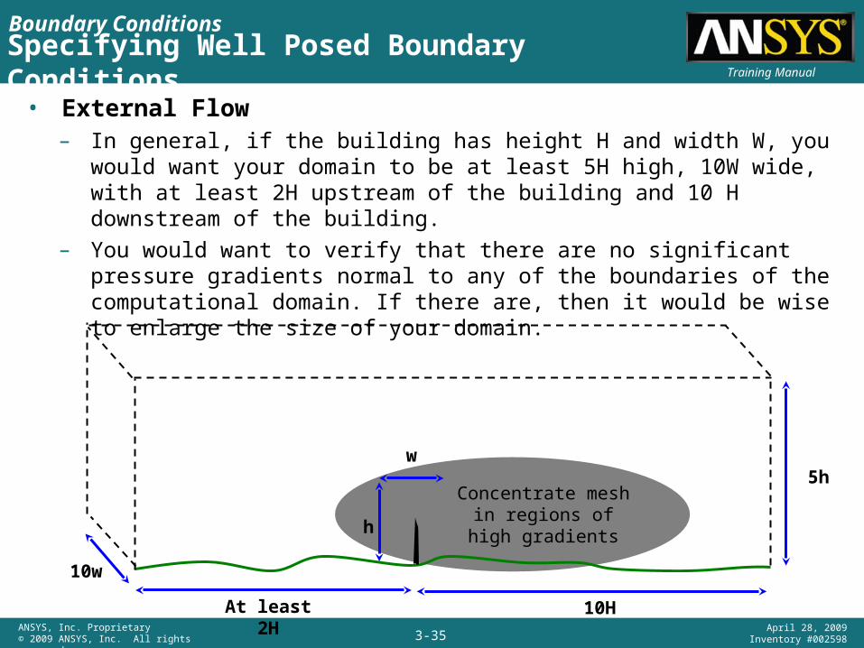
• External Flow– In general, if the building has height H and width W, you would want your
domain to be at least 5H high, 10W wide, with at least 2H upstream of the building and 10 H downstream of the building.
– You would want to verify that there are no significant pressure gradients normal to any of the boundaries of the computational domain. If there are, then it would be wise to enlarge the size of your domain.
Specifying Well Posed Boundary Conditions
w
h
5h
10HAt least 2H
10w
Concentrate mesh in regions of high
gradients
Boundary Conditions
3-36ANSYS, Inc. Proprietary© 2009 ANSYS, Inc. All rights reserved.
April 28, 2009Inventory #002598
Training Manual
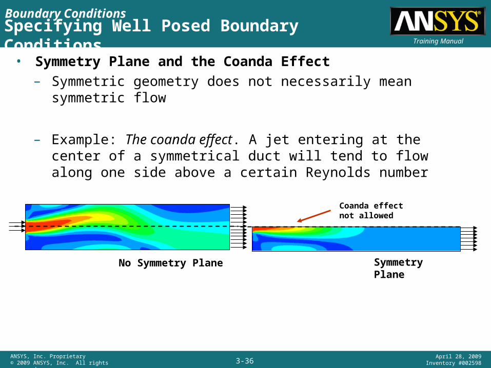
• Symmetry Plane and the Coanda Effect– Symmetric geometry does not necessarily mean symmetric flow
– Example: The coanda effect. A jet entering at the center of a symmetrical duct will tend to flow along one side above a certain Reynolds number
Specifying Well Posed Boundary Conditions
No Symmetry Plane Symmetry Plane
Coanda effect not allowed
Boundary Conditions
3-37ANSYS, Inc. Proprietary© 2009 ANSYS, Inc. All rights reserved.
April 28, 2009Inventory #002598
Training Manual
• When there is 1 Inlet and 1 Outlet– Most Robust: Velocity/Mass Flow at an Inlet; Static Pressure at an Outlet.
The Inlet total pressure is an implicit result of the prediction.
– Robust: Total Pressure at an Inlet; Velocity/Mass Flow at an Outlet. The static pressure at the Outlet and the velocity at the Inlet are part of the solution.
– Sensitive to Initial Guess: Total Pressure at an Inlet; Static Pressure at an Outlet. The system mass flow is part of the solution
– Very Unreliable: Static Pressure at an Inlet; Static Pressure at an Outlet. This combination is not recommended, as the inlet total pressure level and the mass flow are both an implicit result of the prediction (the boundary condition combination is a very weak constraint on the system).
Specifying Well Posed Boundary Conditions
Boundary Conditions
3-38ANSYS, Inc. Proprietary© 2009 ANSYS, Inc. All rights reserved.
April 28, 2009Inventory #002598
Training ManualSpecifying Well Posed Boundary Conditions
• At least one boundary should specify Pressure (either Total or Static)– Unless it’s a closed system– Using a combination of Velocity and Mass Flow conditions at all boundaries
over constrains the system
• Total Pressure cannot be set at an Outlet– It is unconditionally unstable
• Outlets that vent to the atmosphere typically use a Static Pressure = 0 boundary condition
– With a domain Reference Pressure of 1 [atm]
• Inlets that draw flow in from the atmosphere often use a Total Pressure = 0 boundary condition (e.g. an open window)
– With a domain Reference Pressure of 1 [atm]
Boundary Conditions
3-39ANSYS, Inc. Proprietary© 2009 ANSYS, Inc. All rights reserved.
April 28, 2009Inventory #002598
Training ManualSpecifying Well Posed Boundary Conditions
• Mass flow inlets result in a uniform velocity profile over the inlet– Fully developed flow is not achieved– You cannot specify a mass flow profile
• Mass flow outlets allow a natural velocity profile to develop based on the upstream conditions
• Pressure specified boundary conditions allow a natural velocity profile to develop