case study of gis data integration and visualization

Goldfinger et al., Marine Geodesy v. 20, p. 267-289, 1997

Case Study of GIS Data Integration And Visualization in Marine Tectonics:

The Cascadia Subduction Zone

CHRIS GOLDFINGER College of Oceanic and Atmospheric Sciences Oregon State University Corvallis Oregon 97331 LISA C. MCNEILL Department of Geosciences Oregon State University Corvallis Oregon 97331 CHERYL HUMMON Department of Geosciences Oregon State University Corvallis Oregon 97331

A raster/vector GIS has been developed at the College of Oceanic and Atmospheric Sciences at Oregon State University to support investigations of the active tectonics and earthquake potential of the Cascadia subduction zone. The Cascadia marine GIS uses Erdas Imagine as its core display and database software. Supporting software includes specialized processing packages for multibeam bathymetric data, deep-towed sidescan sonar data, file conversion, and 3D stereo visualization. The GIS is used in all phases of the Cascadia project, including assessment of target sites for submersible and sidescan fieldwork, submersible and towfish navigation, and visualization and interpretation. The GIS, along with its supporting components, is used in interpretation of geologic structure, a highly interpretive and largely visual process. The integration of geologic, geophysical, and morphologic data has led to the determination of slip-rates of offshore faults, an estimate of the potential seismogenic zone on the Cascadia subduction thrust, and the discovery of massive failure of the continental slope off southern Oregon.

Received 23 February 1996; accepted 8 June, 1996. Keywords GIS, 3D visualization, active tectonics, sidescan sonar, multibeam bathymetry Introduction Although the use of GIS on land is commonplace, and the use of GIS for tectonic studies is becoming more common, GIS is a relative newcomer to tectonic investigations in the marine environment. In the marine environment, there have emerged few standard data formats,


datasets are large, and are often collected and processed with customized software packages, inhibiting the use of commercial GIS systems. Commercial GIS packages are driven by economics, and thus are geared toward data in standardized raster and vector formats for the most used land-base applications. Nevertheless, GIS is a useful tool for integrating various forms of marine data allowing geologic interpretation with the aid of integrated datasets in a geographic context (e.g. Hatcher, 1992; Li and Saxena, 1993; Wright et al., in press). In this paper, we describe a case study of the integration of marine data in a long term study of the active tectonics of the Cascadia subduction zone off the Pacific Northwest coasts of Oregon and Washington. Similar methods have been used GIS for landslide and hazard mapping (e.g. Rengers et al., 1992; Leroi et al., 1992 ), marine field studies (e.g. Li and Saxena, 1993; Hatcher, 1992; Wright et al., in press; Hall et al., 1995), and underwater search operations (e.g. Caswell, 1992). The project began as a mapping project in which seismic reflection data was to be used to map active folds and faults on the Oregon margin. The trackline maps for the reflection profiles were digitized and plotted at 1:500,000 scale. The structural map was constructed on a mylar sheet overlaying the trackline maps. Midway through this initial phase, we were overwhelmed by the enormous quantity of data and the daunting task of mapping 80,000 km2 of the continental margin using about 30,000 km of seismic profiles (Figure 1). The first step toward data integration was to complete the initial mapping on a CAD system, vastly improving the mapping procedure and making the map less scale dependant. When multibeam bathymetric data became available on the Oregon margin, the CAD system was soon outclassed and GIS became the only viable way to integrate the interpretation of seismic reflection data and high-resolution bathymetry. We acquired a raster/vector GIS system (ERDAS Imagine) that emphasized raster data manipulation and analysis, with a vector data model compatible with other systems in common usage (Arc/Info). With the introduction of a GIS to the project, we integrated several types of sidescan sonar imagery, gravity, magnetics, core, well and dredge sample locations, and submersible tracks. The Cascadia GIS now consists of about 20 GB of imagery, bathymetry and vector data. While the GIS made it possible to store, view, and make maps using any combination of the georeferenced datasets, we found that GIS could not do everything. The inherent 2D layering of most GIS systems limited use of the third dimension, and the vector capabilities fell far short of the CAD system (Intergraph Microstation) we were already using. Visualization capabilities in most GIS systems also lagged far behind state of the art visualization packages. We also found that land-oriented GIS systems were incapable of processing and georeferencing marine multibeam bathymetric and sidescan sonar data. Conversely, software available for processing these data were not oriented toward integration with a GIS system. To accomplish our scientific goals, we use the GIS as the central database for viewing and manipulating final or near final data products created in CAD, visualization, and specialized data processing software. In the following sections we describe the development and use of the Cascadia marine GIS system. Our goal was to support continuing tectonic studies of the continental margin, not to develop innovative software or data structures. As such, we made as much use as possible of off the shelf software, and only developed custom applications when nothing suitable existed, or to bridge the gaps between existing packages.


Figure 1. Partial trackline map showing seismic reflection tracklines used in the Cascadia GIS. The shotpoints for all lines are in vector layers, which are used with the seismic records and bathymetry layers for on-screen mapping.


The Cascadia Subduction Zone Project And GIS System The Cascadia subduction zone is a convergent margin at which the oceanic Juan de Fuca and Gorda plates subduct beneath the continental North American plate off the coast of northern California, Oregon, Washington, and Vancouver Island (Figure 2). To date, no historic earthquakes have been recorded on the plate interface (Ludwin et al., 1991), leading early researchers to conclude that subduction had either stopped or was aseismic (Ando and Balazs, 1979; West and McCrumb, 1988). Geologic evidence (Kulm and Fowler, 1974; Barnard, 1978) proves that the former cannot be true and onshore evidence suggests that large subduction earthquakes have occurred during the Holocene (Figure 2; Atwater, 1987; Atwater et al., 1995; Nelson et al., 1995). The magnitude and rupture location of a potential subduction zone earthquake on the Cascadia subduction zone is still hotly debated. During the last 5 years, our research has focused on identifying active (within the last 1 Ma) faults of the submarine Cascadia forearc and the subducting Juan de Fuca plate. We have been using remote and geophysical methods to characterize the style and rate of deformation of both converging plates in order to assess the seismic potential of the Cascadia plate boundary. Data Collection And Near Real Time Processing New data collected for this project consisted principally of sidescan sonar, multibeam bathymetry, video and still images, and observations and samples from shallow and deep-diving submersibles. In 1993, we collected deep-towed SeaMARC 1A sidescan sonar data and Hydrosweep multibeam bathymetry on the continental slope and abyssal plain off Oregon and Washington. A significant part of the data was collected during a series of cruises on the Oregon and Washington continental shelf and upper slope region using the shallow-diving submersible DELTA in conjunction with AMS-150 kHz sidescan sonar. Prior to each cruise, targets relevant to the project, such as active faults, were identified from the existing database of seismic reflection data. At sea, we employed the sidescan sonar at night to survey the target area, simultaneously collecting bathymetric data. DELTA was then used to collect field observations and samples from the target sites, providing both detailed geologic field relationships and "ground truthing" of the sonar imagery. Since our targets were both numerous and geographically separated, limited time and resources were available for each target. This cruise format allowed good utilization of ship time, but created a challenge in that the pace of operations required rapid processing and assimilation of data in order to plan upcoming dives and sonar surveys. Sonar Surveys We used a deep water SeaMARC 1A (30 kHz) system for work on the continental slope and abyssal plain, and an AMS 150SI (150 kHz) system on the continental shelf and upper slope. The SeaMARC 1A system can collect a 5 km or 2 km swath width and collects 2048 pixels per ping, giving across track pixel sizes of 0.97 m and 2.4 m respectively. We used a 1 km swath with the AMS 150, yielding an across track pixel size of 0.49 m. The actual resolution of final imagery of these and other sidescan systems is a complex function of acquisition, system, and image processing parameters (Johnson and Helferty, 1990). Initial processing of the sidescan data carried out during acquisition consisted of slant-range correction, and a time-varying gain (TVG) correction for spherical spreading of the signal. During much of the 1993 cruise off the Washington coast, we were conducting reconnaissance surveys of active faults in areas for which no detailed bathymetry is available.


Figure 2. Active tectonic map of the Oregon-Washington continental margin. Faults and anticlines shown; synclines deleted for clarity. JDF-NOAM vector of DeMets et al. (1990) is shown. Dashed line is inferred edge of Siletzia terrane based on magnetics and reflection-refraction data. Strike-slip faults, shown with slip rates in mm/yr: NNF = North Nitinat fault; SNF = South Nitinat fault; WCF = Willapa Canyon fault; WF = Wecoma fault; DBF = Daisy Bank fault; ACF = Alvin Canyon fault; HSF = Heceta South fault; CBF = Coos Basin fault; TRF = Thompson Ridge fault. NF = Nitinat Fan; AF = Astoria Fan. Major depocenters shown in stipple: WB = Willapa Basin; AB = Astoria Basin; NB = Newport Basin; CBB = Coos Bay Basin. Submarine Banks: NB = Nehalem Bank; HB = Heceta Bank; CB = Coquille Bank. All offshore seismicity from composite catalog is shown, with Blanco Fracture Zone and Gorda plate events removed. Selected marsh burial sites from Atwater et al. (1995) are shown.


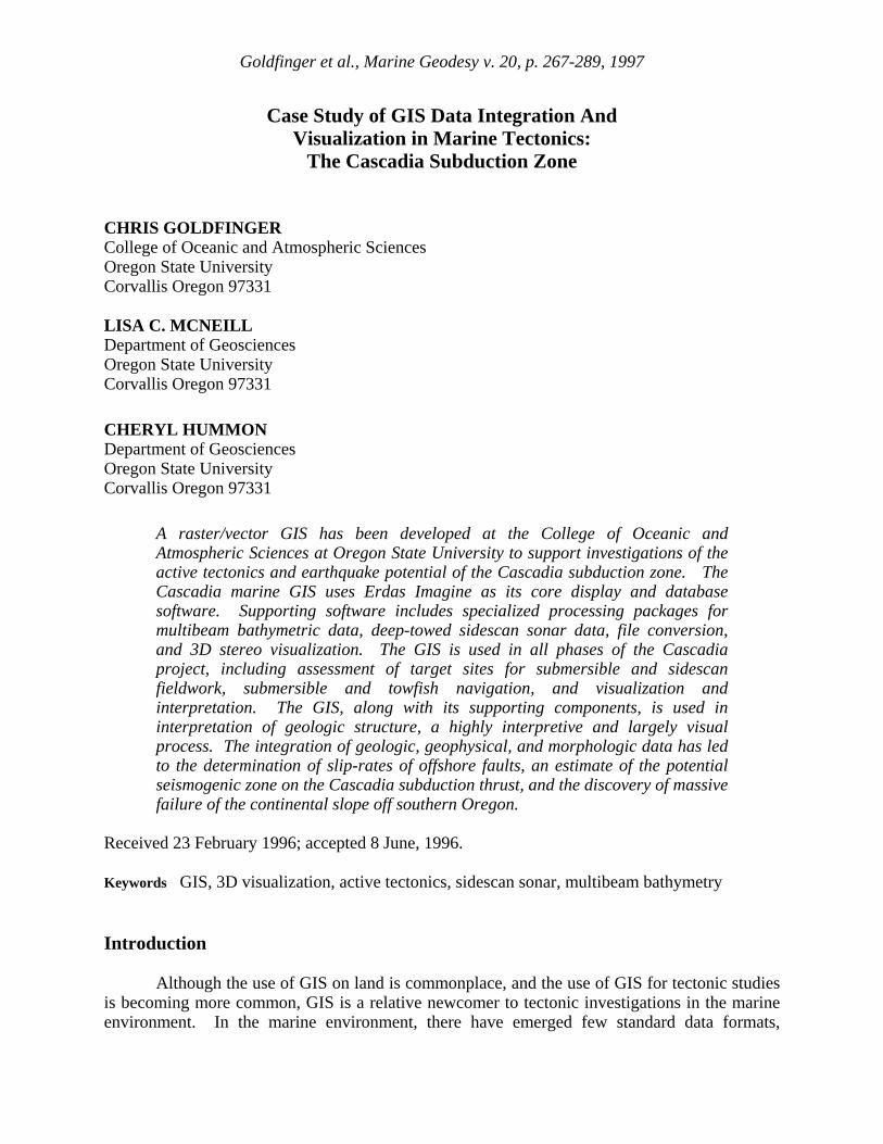
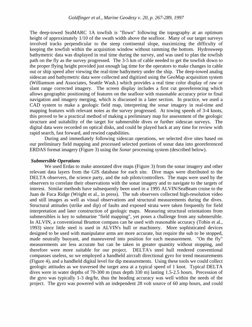
The deep-towed SeaMARC 1A towfish is "flown" following the topography at an optimum height of approximately 1/10 of the swath width above the seafloor. Many of our target surveys involved tracks perpendicular to the steep continental slope, maximizing the difficulty of keeping the towfish within the acquisition window without ramming the bottom. Hydrosweep bathymetric data was displayed in real time during the survey, and was used to plan the towfish path on the fly as the survey progressed. The 3-5 km of cable needed to get the towfish down to the proper flying height provided just enough lag time for the operators to make changes in cable out or ship speed after viewing the real-time bathymetry under the ship. The deep-towed analog sidescan and bathymetric data were collected and digitized using the GeoMap acquisition system (Williamson and Associates, Seattle Wash.) which provides a real time color display of raw or slant range corrected imagery. The screen display includes a first cut georeferencing which allows geographic positioning of features on the seafloor with reasonable accuracy prior to final navigation and imagery merging, which is discussed in a later section. In practice, we used a CAD system to make a geologic field map, interpreting the sonar imagery in real-time and mapping features with relevant notes as the survey progressed. At towing speeds of 3-4 knots, this proved to be a practical method of making a preliminary map for assessment of the geologic structure and suitability of the target for submersible dives or further sidescan surveys. The digital data were recorded on optical disks, and could be played back at any time for review with rapid search, fast forward, and rewind capabilities. During and immediately following sidescan operations, we selected dive sites based on our preliminary field mapping and processed selected portions of sonar data into georeferenced ERDAS format imagery (Figure 3) using the Sonar processing system (described below). Submersible Operations We used Erdas to make annotated dive maps (Figure 3) from the sonar imagery and other relevant data layers from the GIS database for each site. Dive maps were distributed to the DELTA observers, the science party, and the sub pilots/controllers. The maps were used by the observers to correlate their observations with the sonar imagery and to navigate to the targets of interest. Similar methods have subsequently been used in a 1995 ALVIN/SeaBeam cruise to the Juan de Fuca Ridge (Wright et al., in press). The sub observers collected high-resolution video and still images as well as visual observations and structural measurements during the dives. Structural attitudes (strike and dip) of faults and exposed strata were taken frequently for field interpretation and later construction of geologic maps. Measuring structural orientations from submersibles is key to submarine "field mapping", yet poses a challenge from any submersible. In ALVIN, a conventional Brunton compass can be used with reasonable accuracy (Tobin et al., 1993) since little steel is used in ALVIN's hull or machinery. More sophisticated devices designed to be used with manipulator arms are more accurate, but require the sub to be stopped, made neutrally buoyant, and maneuvered into position for each measurement. "On the fly" measurements are less accurate but can be taken in greater quantity without stopping, and therefore were more suitable for our project. DELTA's steel hull rendered conventional compasses useless, so we employed a handheld aircraft directional gyro for trend measurements (Figure 4), and a handheld digital level for dip measurements. Using these tools we could collect geologic attitudes as we traversed the target area at a typical speed of 1 knot. Typical DELTA dives were in water depths of 70-300 m (max depth 330 m) lasting 1.5-2.5 hours. Precession of the gyro was typically 1-3 deg/hr, thus the heading accuracy was well within the needs of the project. The gyro was powered with an independent 28 volt source of 60 amp hours, and could


Figure 3. Dive map from DELTA dive 3040 at Stonewall Bank on the central Oregon continental shelf. The dive site is a region of exposed east-dipping Miocene strata that were incised by a late Pleistocene subaerial channel during the Wisconsin sea-level lowstand. The dive map is carried in the submersible, and used as a backdrop for real-time plotting of sub position using the Seaview application. last an entire dive day (3-6 dives) with negligible voltage drop. We calibrated the handheld gyro with the ships gyro before and after each dive to monitor the precession of the instrument. During the dives, the same digital dive map was used as a backdrop for real-time plotting of submersible position. Sub position was derived by merging DGPS ship position with range and bearing information from a Trackpoint (ORE Industries) ultrashort baseline system. The sub position fixes were then plotted every two seconds on the sidescan dive map using Seaview, an application modified from an existing program written by the Woods Hole Oceanographic Institution Deep Submergence Group. If bathymetric data are available in advance, navigation plotting can also be done using a companion 3D program, with sidescan imagery draped over the bathymetry. This real-time display on the support vessel, in conjunction with dive maps in the submersible, proved to be adequate to locate and investigate targets without the need for bottom transponder deployment, greatly speeding data collection and increasing flexibility and efficiency. Bathymetry Post-Processing Bathymetric data are a key layer in the Cascadia GIS database. The morphology of the actively deforming continental margin is a direct result of faulting and folding, with modification by sedimentation and erosion. Therefore, the best possible bathymetric/topographic base is


Figure 4. Aircraft electric directional gyro used in the DELTA submersible for collecting structural orientations of bedding planes and fault surfaces. The gyro is set by the ship's gyro prior to a dive. The unit is hand-held and used to sight along the strike plane of bedding or a fault while reading the heading indicator. Dip was measured using a digital level in the same manner. These measurements were within ~5° of true strike. essential to understanding the map view and/or three-dimensional nature of a tectonically active region. Several commercial and public domain software packages can process multibeam bathymetric and coincident backscatter data, which are collected with ship mounted or shallow towed systems. We used the MB System software available from Lamont Doherty Geological Observatory to process Hydrosweep data collected during this project. Navigation is relatively straightforward in that ship position and sensor position are usually the same, allowing simple merging of ship navigation data with the ping files of depth/backscatter collected by the multibeam system. Compensation for motion of the platform is usually integrated into the acquisition software/hardware of newer systems, such as Hydrosweep and SeaBeam 2000 series instruments, but must be corrected for in post processing with older systems . The merging process considers the effects of the velocity structure of the water column on the path of each beam. Calculation of the position of each beam is done using a water velocity model derived from actual casts or from historical water mass data. A file is generated of X, Y and depth, which is then gridded and incorporated in GIS and visualization software, discussed in a later section. Bathymetric data were also collected from deep-towed vehicles while simultaneously collecting sidescan sonar imagery using an isophase interferometric technique. This type of bathymetry is derived from the same signal as the sonar imagery by two sets of parallel transducers mounted on each side of the towfish. The parallel transducers detect phase differences in the received pulse, from which the return angle to the transducers, and therefore depth, can be calculated using the two-way travel time of the signal and the known water velocity (e.g. Reed and Hussong, 1989).


Deep-Towed Sidescan Sonar Post-Processing Deep-towed sidescan sonar systems have much greater resolution than surface-towed or hull mounted systems, and are thus needed in mature field areas where regional data already exist. The processing of deep-towed sidescan sonar data, however, is more complex than that of multibeam bathymetric data. The spatial aspects of deep-towed sidescan data processing are essentially similar to bathymetry processing, described above, but with the added complications of the sensor traveling a "water skier" path behind the vessel, and having a pitch, roll, and yaw that must be considered during processing. Water velocity effects, however, are minimized because of the short travel path between the towfish and the bottom, which also minimizes the raypath bending in a stratified water column. Positioning of the towfish is critical not only in placing features in their correct position on the seafloor, but for producing visually usable imagery. We found processing software for this type of data was rare, and what existed did not read the data formats we worked with, or output useful formats for GIS. We therefore elected to write our own processing package, Sonar, the sole case where off the shelf software did not substantially meet our needs. Since we anticipated a multiyear data collection effort, this proved worthwhile and we were able to incorporate the processing algorithms and file formats we needed. Complete descriptions of sidescan sonar processing techniques and algorithms are beyond the scope of this paper (see Reed and Hussong, 1989; Johnson and Helferty, 1990; De Moustier and Matsumoto, 1993). The Sonar package takes two files as input: (1) slant-range corrected sonar backscatter data files with included towfish attitude, depth, altitude, and heading telemetry; and (2) towfish navigation files. Towfish navigation can be provided by several methods. Ultrashort baseline tracking systems (e.g. Edwards, 1989) that merge the ship's position (GPS or DGPS) with range and bearing to the towfish derived from a "pinger" are the simplest for shallow to moderate water depths. For deep water surveys, a medium length baseline system using bottom transponders well suited for precision surveys, but has the disadvantage of considerable overhead time in setting and recovering transponders. Towfish position can also be calculated from ship position with reasonable accuracy for reconnaissance surveys. We employed this method for SeaMARC 1A surveys in deep water where the cable length exceeded the range of pingers, and where our survey targets were numerous and widely separated, making bottom transponder deployment impractical. The algorithm employed in the Sonar program uses cable out, towfish speed, heading, altitude, and depth, wire catenary, and ship heading and turn rate to calculate towfish position. Post-processing tests of this algorithm by comparison with GPS navigated multibeam bathymetry proved that this method could place the towfish with sufficient accuracy such that errors relative to the bathymetry were not detectable. Suitability of this technique requires negligible ocean currents for good results. Image processing steps carried out during post-processing can vary, but usually included a histogram correction dependant on the characteristics of the sonar system, a routine to adjust intensity values for occasional bad pings with skewed gain, and an intensity correction to produce a flat across track average pixel intensity profile. The latter correction helps to remove the across track intensity variations that often dominate mosaics with many parallel swaths. Other settable parameters from the user interface include smoothing windows for towfish altitude, attitude, grid node spacing, and selectable grid search methods. The processing system can distribute processing jobs to different machines over a network, and we typically make use of an IBM RS-6000/SP-2 cluster of 10 CPU's. The processing software has been used on Sun, SGI, IBM RS-6000/SP2 and Linux/PC platforms.


Figure 5. SeaMARC 1A sidescan sonar image of the intersection of the North Nitinat fault and the plate boundary off the central Washington coast. Light tones are high backscatter. Fault offsets the landward-vergent thrust ridge, slump debris, slump headwall scarps, and an abyssal plain channel. The fault is not offset laterally at the plate boundary thrust. Swath width 5 km. Lower panel shows interpretation of the sidescan image. A local 20° bend in the strike of accretionary wedge anticlines occurs across the fault, which widens and branches into multiple traces east of the deformation front. Extensive slumping of the backlimb of the landward-vergent frontal anticline of the accretionary wedge may be triggered by strike-slip faulting. Two episodes of slumping are indicated by the glide paths of the younger slump blocks which have overridden earlier slump debris. Some interpretation details are based on 3-D stereo visualization of the imagery and co-registered swath bathymetry. Output from the Sonar program is georeferenced gray-scale imagery in Erdas Imagine format which requires no further post processing or conversion to be used in the GIS system (Figure 5). Simultaneous output is also available in Sun raster and raw RGB formats. The Sun raster output, and an associated header file generated by Sonar, are used directly by the Seaview real-time navigation plotting software discussed previously. The RGB image format is used by a 3D visualization system discussed in a following section.


GIS And Visualization For Tectonic Applications Integration Of Data The current GIS database for Cascadia Subduction Zone tectonics consists of published datasets and data collected during NSF and NOAA/NURP (National Undersea Research Program) sponsored offshore fieldwork. The GIS database, in Erdas Imagine 8.2, is continually updated as new data becomes available. Publicly available datasets include: swath bathymetry; seismicity catalogs; GLORIA (Geologic LOng Range Inclined Asdic) sidescan sonar imagery; USGS 3 arc-second digital elevation models (DEM); gravity and magnetic anomaly data; seismic reflection survey tracklines; published geologic maps; and DSDP/ODP drill hole data. Data collected specifically for Cascadia neotectonic-related studies include: sidescan sonar data collected between 1989 and 1995; Hydrosweep swath bathymetry of key areas of the Washington margin; sample sites including box cores, piston cores, dredge hauls, and submersible samples; submersible tracks from fieldwork between 1989 and 1995; and offshore neotectonic and lithologic maps. Bathymetry of the Oregon continental margin and abyssal plain has been gridded with onshore 3' DEM's obtained from the U.S. Geological Survey, with 100m and 300m grid centers. Bathymetric data of the continental slope, between water depths of 600 and 3000 m, were collected during the Deep Water SeaBeam surveys of the EEZ Bathymetric Mapping Program (1984 - 1992) conducted by NOAA (National Oceanic and Atmospheric Administration) and NOS (National Ocean Service), (Lockwood and Hill, 1989). Some areas of the outer continental shelf and upper slope (150-600m water depths) were surveyed with a shallow water 36 kHz multibeam system (BSSS; S. Mutula, NOAA, pers. comm. 1993). The BSSS data have been made available to the OSU group and have been incorporated into the 100m grid. SeaBeam multibeam bathymetric surveys conform to International Hydrographic Organization standards, which require a 75m maximum horizontal positioning error and sounding depth accuracy within 1% of the water depth. The horizontal circular position error of the EEZ survey is 50m. Navigation for the EEZ bathymetric data used a shore-based ARGO DM-54 navigation system. Comparisons with a 1989 Digicon multichannel seismic reflection survey of the northern Oregon continental slope, which utilized a continuous commercial satellite navigation system, shows good positional agreement. Continental shelf bathymetry consists of digitized contours from NOS publications that were regridded using a continuous curvature splines in tension routine in the GMT plotting software package (Smith and Wessel, 1990). Additional SeaBeam data was collected on the N. California continental slope by NOAA in 1995 (C. Fox, NOAA PMEL, pers, comm. 1995) which has also been incorporated into the GIS database. An unmapped region remains on the northern California margin which we hope to complete in 1997 using the SeaBeam 2000 system. Currently, multibeam bathymetric data on the Washington margin is classified by the U.S. Navy. We plan to extend our 100 m bathymetric grid to include the entire Cascadia subduction zone, from offshore northern California to Vancouver Island, using the best available data on the Washington margin. We use both the raw height data and shaded relief imagery as separate layers in our GIS. The height data can be used for slope profiling, stream profiling along submarine channels, and for generation of slope and aspect maps, also discussed below. Profiling of submarine channels can lead to determination of deformation rates, since active growing folds deform the thalweg profile, which can in some instances be dated with core samples (Figure 6; Goldfinger et al., 1992). The shaded relief imagery is used to make correlations of structures that have topographic relief between seismic profiles, and to identify and interpret the tectonic geomorphology of active folds and faults (Figures 2 and 7).


Figure 6. Shaded-relief NOAA SeaBeam bathymetry (100m grid) of the Astoria canyon and channel on the lower continental slope and abyssal plain, N. Oregon. The canyon thalweg is deformed by active accretionary wedge structures, as shown on the bathymetric profile (B-B') along the thalweg. The deformation front steps to the right on a NE-trending fault (F) that deforms the Astoria canyon. Three landward-vergent anticlines (A1, A2, A3), also deform the canyon floor. The steep canyon walls are prone to collapse or slumping; the debris pile from one slump (S) is visible on the bathymetric profile. Gridded gravity and magnetic anomaly data from the Decade of North American Geology (DNAG) geophysical dataset have been incorporated into the Cascadia GIS database. However, these data were found to have a significant shift in position relative to known bathymetric features and individual ship track data. The nature and magnitude of this shift have not entirely been resolved as of this writing. Gridded bathymetric, gravity, and magnetics data provide raster basemaps for our georeferenced multilayer Cascadia GIS database. Additional raster layers include sidescan sonar images: GLORIA long-range sidescan collected as part of the EEZ project throughout the Cascadia continental slope (EEZ-SCAN 84 Scientific Staff, 1988); deep-towed SeaMARC-1A 30 kHz sidescan on the Oregon and Washington continental slope, and AMS 150 kHz sidescan on the Oregon and Washington continental shelf. Individual high-resolution sidescan images can be mosaiced and displayed in any overlapping order. GLORIA sidescan data was mosaiced and georeferenced by USGS (EEZ-SCAN 84 Scientific Staff, 1988). We have used multibeam bathymetric data where appropriate to georeference the GLORIA data to these reliably-navigated datasets for consistency within our database. Published geologic maps of the coastal and


offshore regions of Oregon and Washington have been scanned and georeferenced as raster layers within the Cascadia database. Vector layers within Erdas can be overlain on the aforementioned raster layers allowing interpretation of spatial relationships. Vector layers include: sample sites; tracklines of seismic reflection surveys; structural and geologic maps; submersible dive and sidescan tracks; and seismicity data. Seafloor samples (dredge hauls, box cores, submersible grabs, etc.) in the northeast Pacific have been collected and stored at OSU in the COAS Core Laboratory. Grouped sampling sites are represented as vector layers, with associated attribute tables providing information on sample ID, latitude, longitude, sample lithology, sample type (core, grab, submersible, etc), water depth, and paleo-water depth and sample age where available (Table 1). In addition, locations and attributes of Deep Sea Drilling Project (DSDP) and Ocean Drilling Program (ODP) sites and oil-exploratory wells are stored as vector layers. Our non-digital database includes all publicly available industry, government, and academic seismic reflection profiles. Shotpoint location maps are stored within the GIS as additional vector layers. This allows cross-correlation with the seismic reflection profiles, which are a hardcopy dataset independent of the GIS. The large number of records and lack of intrinsic 3D spatial capability in ERDAS preclude the inclusion of seismic reflection profiles as digital data in the GIS. Only a small fraction of these data are available in digital form, the majority are paper records which would have to be scanned, requiring resources beyond the scope of the project. Submersible tracklines are separated and stored according to the year of fieldwork, allowing differentiation between individual study areas and the ability to cross-correlate with data stored outside the GIS database. Each submersible dive has an associated videotape and textual record of measurements and observations made by the observer as well as photographic data, and sediment and rock samples. The trackline vector layers are presently time coded to key sample sites to these external databases. Using the ArcView display software, these sample sites can be linked directly to sample video clips, still images, or other visual or tabular data so that an investigator can simply click on a point along the submersible track to display relevant data or imagery from that sample site. A seismicity layer has been compiled from all publicly available catalogues: ISC/Harvard; PNSN; NEIC; NCSN; and additional SOSUS (SOund SUrveillance System) hydrophone array T-phase events from NOAA with a minimum resolvable magnitude of 2 (Fox et al., 1993). The seismicity vector layer can, to some extent, be overlain on the neotectonic map to identify which faults are seismically active. The events recorded by onshore seismic networks are not well located due to the poor azimuthal station coverage of the land networks for offshore events. The NOAA SOSUS data give excellent locations, and can be used to relocate events recorded on land, thus comparisons of seismicity to structures in Cascadia will become a more useful technique as time goes on (C. Fox, R. Dziak, pers. comm., 1996). Stereo And Real-Time Fly-Through Visualization Visualization is one of the most important techniques available to geologists. This is even more so in tectonic geomorphology, the study of active faults and the morphology they create. As Van Driel (1989) pointed out, a plot of elevations does little to aid the brain in interpretation, while a contour plot is a little better, but still requires most of our interpretive powers to simply see the represented surface. Wireframe plots are better still, but a shaded relief surface plot presents all the data in a form easily interpretable to the geologist. Best of all is a shaded relief plot, viewable from any angle with variable light source direction and incidence angle.


Three-dimensional visualization of single or multiple GIS datasets can be performed in Erdas Imagine and Fledermaus, a real-time fly-through visualization tool developed by Larry Mayer (Interactive Visual Systems, New Brunswick). The Perspective View function in Erdas can be used to view datasets of x, y, z data, such as topography layers, with additional overlain raster layers, such as sidescan and/or shaded relief bathymetry. The overlain raster layers must be in the same projection as the underlying topographic layer, but may have different resolution and coverage than the height data, a powerful feature. These combined datasets can then be viewed from any direction while controlling the viewpoint height, vertical exaggeration, and angle and direction of illumination. Drawbacks are that the display is not interactive, and must be redrawn for any change in settings, nor can other objects be displayed in relation to the height data and overlaid raster image. Fledermaus also allows three-dimensional and stereo visualization, but can be used, in addition, to fly through the datasets in real time. A shaded relief surface image is produced and displayed in 3D with gridded height data. Fledermaus uses a binary grid which can be generated from xyz data. Gridded height data is then incorporated with a raw RGB image file to produce a shaded relief image of the height data. The image can be edited by adding annotations within a suitable graphics package or merging with other image files such as overlaid sidescan sonar imagery (Figure 8). Fledermaus can be used in a "turntable" mode, where the mouse is used to rotate and adjust the view of the data objects. Coupled with a 6 degree of freedom mouse or "bat" (up, down, right, left, roll, pitch, yaw), one can "fly" through and around data objects at will, directing the pointing device in relation to the data as if it were a toy airplane. Fledermaus was designed to handle large datasets with the speed required for real-time fly-throughs (Paton, 1995). Fly-throughs can be done in stereo mode, using LCD shutter glasses triggered by the computer to show the viewer's eyes rapidly alternating right and left views, producing the stereo effect. Fledermaus can also display digital seismic reflection data, cable routes, and time series data as 3D objects that can be georeferenced. Stereo and 3D images permit structural interpretations that cannot be made in two dimensions. In particular, identification of topographic and structural features in sidescan sonar images is often complicated by the variation in reflectivity produced by different surface lithologies. For example, a facing slope has high acoustic reflectivity but can be confused with an area of high reflectivity material such as calcium carbonate. Complex procedures can sometimes be applied to the sidescan data to separate these effects (e.g. Carson et al., 1994). However, by overlaying georeferenced sidescan sonar images on topographic data and viewing in 3D, structurally-related topography is clearly revealed (Figure 8), frequently reducing the need for complex assumption-based secondary processing. These techniques allow the observation of subtle features upon which tectonic geomorphology is dependent, and the complex inter-relationships between topographic features and fault geometry to be resolved. Geologic Results Structural Geology and Interplate Earthquake Potential Until fairly recently, subduction zones have been viewed with an emphasis on 2D cross sections perpendicular to the margin. This view was the result of widely spaced seismic reflection profiles that could not be correlated very far in any direction with other profiles, or othert datasets. A cross section view does little to address structures parallel to or at angles to the margin, which are particularly important in obliquely convergent settings like the Cascadia subduction zone. The integration of multiple datasets into the Cascadia GIS database and the


Figu

re 7

. St

ruct

ure

map

of t

he w

este

rn p

ortio

n of

the

Wec

oma

faul

t and

fron

tal a

ccre

tiona

ry w

edge

. St

ruct

ure

com

pile

d fr

om m

igra

ted

and

unm

igra

ted

seis

mic

refle

ctio

n pr

ofile

s, Se

aBea

m b

athy

met

ry, A

LVIN

obs

erva

tions

, and

Sea

MA

RC

1A

si

desc

an im

ager

y. A

= in

ters

ectio

n of

"po

p-up

" st

ruct

ure

with

the

Wec

oma

faul

t; PU

= p

op-u

p; P

R =

pre

ssur

e rid

ge

antic

line;

OC

= o

ffse

t cha

nnel

; OS

= of

fset

slum

p sc

ar.

Figu

re 7

. St

ruct

ure

map

of t

he w

este

rn p

ortio

n of

the

Wec

oma

faul

t and

fron

tal a

ccre

tiona

ry w

edge

. St

ruct

ure

com

pile

d fr

om m

igra

ted

and

unm

igra

ted

seis

mic

refle

ctio

n pr

ofile

s, Se

aBea

m b

athy

met

ry, A

LVIN

obs

erva

tions

, and

Sea

MA

RC

1A

si

desc

an im

ager

y. A

= in

ters

ectio

n of

"po

p-up

" st

ruct

ure

with

the

Wec

oma

faul

t; PU

= p

op-u

p; P

R =

pre

ssur

e rid

ge

antic

line;

OC

= o

ffse

t cha

nnel

; OS

= of

fset

slum

p sc

ar.


Tabl

e 1.

Vec

tor a

ttrib

ute

tabl

e fr

om O

SU c

ore

sam

ples

from

the

cont

inen

tal s

helf.

Sam

ples

may

be

sele

cted

by

one

or m

ore

attri

bute

, in

clud

ing:

loc

atio

n, d

epth

, sam

ple

type

, lith

olog

ic c

hara

cter

istic

s. A

ttrib

utes

may

als

o be

use

d to

vis

ually

cod

e th

e sa

mpl

es fo

r scr

een

di

spla

y, u

sing

col

ors a

nd sy

mbo

ls.

O

SU_C

OR

ES-I

D L

AT

(DEG

) LA

T (M

IN)

LON

G

(DEG

) LO

NG

(M

IN)

CO

RE_

LAB

-ID

SA

MPL

E TY

PE

D

EPTH

(M

) LI

THO

LOG

Y

LITH

C

OD

E R

OC

K

GR

AV

EL

SAN

D

SILT

C

LAY

1

45

33.6

0 -1

25

02.2

2 W

7710

A-2

0 B

C

1614

si

lt/cl

ay

0001

1 0

0 0

9 45

48

.00

-125

24

.00

007-

007

GC

20

12

silt/

clay

00

011

0 0

0 12

45

28

.80

-125

31

.20

044-

044

GC

24

51

silt/

clay

00

011

0 0

0 14

45

49

.20

-124

51

.00

058-

058

GC

11

89

silt/

clay

00

011

0 0

0 16

45

28

.20

-125

00

.60

064-

064

GC

16

46

silt/

clay

00

011

0 0

0 17

45

10

.80

-125

28

.38

AT9

009-

1 G

C

2644

sa

nd/s

ilt/c

lay

0011

1 0

0 1

18

45

09.0

0 -1

25

26.2

8 A

T900

9-2

GC

26

24

sand

/silt

/cla

y 00

111

0 0

1 19

45

11

.40

-125

26

.40

AT9

009-

3 G

C

2609

sa

nd/s

ilt/c

lay

0011

1 0

0 1

20

45

10.8

0 -1

25

28.4

4 A

T900

9-4

GC

26

81

sand

/silt

/cla

y 00

111

0 0

1 31

45

40

.80

-124

53

.10

W79

05A

-121

G

C

919

clay

00

001

0 0

0 32

45

21

.00

-125

03

.90

W79

05A

-122

G

C

1671

cl

ay

0000

1 0

0 0

33

45

21.0

0 -1

25

19.0

2 W

7905

A-1

23

GC

17

32

clay

00

001

0 0

0 38

45

20

.40

-125

26

.82

W89

08A

-01G

G

C

2400

cl

ay

0000

1 0

0 0

39

45

12.0

0 -1

25

34.8

0 W

8908

A-0

2G

GC

26

74

clay

00

001

0 0

0 40

45

13

.20

-125

34

.50

W89

08A

-03G

G

C

2649

cl

ay

0000

1 0

0 0

41

45

33.6

0 -1

25

03.0

0 W

7710

A-2

1 K

C

1610

si

lt/cl

ay

0001

1 0

0 0

56

45

33.0

0 -1

25

09.4

8 W

7710

A-1

7 M

C

1018

gr

avel

/san

d/si

lt/cl

ay

0111

1 0

1 1

57

45

34.8

0 -1

25

04.0

2 W

7710

A-1

8-1

MC

15

79

silt/

clay

00

011

0 0

0 58

45

34

.80

-125

04

.02

W77

10A

-18-

2 M

C

1579

si

lt/cl

ay

0001

1 0

0 0

59

45

34.8

0 -1

25

04.0

2 W

7710

A-1

8-3

MC

15

79

silt/

clay

00

011

0 0

0 60

45

34

.80

-125

04

.02

W77

10A

-18-

4 M

C

1579

si

lt/cl

ay

0001

1 0

0 0

61

45

35.4

0 -1

25

02.5

2 W

7710

A-1

9-1

MC

15

94

sand

/silt

/cla

y 00

111

0 0

1 62

45

35

.40

-125

02

.52

W77

10A

-19-

2 M

C

1594

sa

nd/s

ilt/c

lay

0011

1 0

0 1

63

45

35.4

0 -1

25

02.5

2 W

7710

A-1

9-3

MC

15

94

sand

/silt

/cla

y 00

111

0 0

1 64

45

35

.40

-125

02

.52

W77

10A

-19-

4 M

C

1594

sa

nd/s

ilt/c

lay

0011

1 0

0 1

7545

4860

125

3690

D10

PC22

14sa

nd/s

ilt/c

lay

0011

10

01


ability to view multiple datasets in a spatial context permits (the scientist) to interpret the submarine geomorphology and view the margin in both cross section and plan view. We use these techniques to assess the tectonic response of the margin to oblique subduction, specifically focusing on earthquake potential. A neotectonic map of the Oregon and Washington margins has been compiled from analysis and interpretation of the above datasets during the last 5 years (Figure 2). Throughout the project, the map has been continually updated as new data becomes available. The Oregon part of the neotectonic map was published in 1992 (Goldfinger et al., 1992a) and the Washington neotectonic map will be published shortly (Figure 2). The map gives the locations of mapped geologic structures, including faults, that can be identified from available data, with particular emphasis on recently active structures. Within the GIS, faults and folds are grouped as layers, which are then further subdivided by age as having been active in the Holocene and Late Pleistocene (<1 Ma), Pleistocene (1.8-1.0 Ma) and pre-Pleistocene. The development and study of this map has enabled us to analyze how the Cascadia continental margin has been deforming under oblique convergence between the Juan de Fuca and North American plates. Of particular interest, are a group of transverse faults with left-lateral offset (Figures 2, 5, and 7) which may geomorphically and/or tectonically divide the margin into segments (Goldfinger, 1994; McCaffrey and Goldfinger, 1995). Structural segmentation of the margin is of particular relevance to earthquake potential of the Cascadia subduction zone, since segmentation is one mechanism that can limit the propagation of rupture along a fault (e.g. Ryan and Scholl, 1993; Yeats et al., in press). The left-lateral faults may also indicate that the submarine forearc is weak, which would act to reduce the maximum subduction earthquake magnitude (McCaffrey and Goldfinger, 1995). Fold trends and spacing have also been used to estimate the location of the well-coupled zone of the plate interface from which plate boundary earthquakes originate (Goldfinger et al., 1992a, Clarke and Carver, 1992). The current version of the neotectonic map is made available in digital form, for Sun, Mac, and PC, at our World Wide Web site (http://pandora.oce.orst.edu) and by anonymous ftp from the same site. Predictive GIS Mapping Recently we performed an analysis of the route of a trans-pacific telephone cable which was deployed prior to the availability of high resolution SeaBeam bathymetry. The object of this study was to analyze areas where cable suspensions above the seafloor might occur along the route (undesirable), and where the cable might drape over hard outcropping rock (also undesirable). A major constraint on this study was that economics did not allow collection of new sidescan sonar data, therefore existing SeaBeam data and low resolution GLORIA sidescan were the only available seafloor datasets. To address these problems, we generated slope and predicted-outcrop maps from the SeaBeam bathymetric data that were used to evaluate problem areas along the cable route. The slope map is a raster layer generated from the height data, and is shaded or colored by slope angle calculated between bathymetric data points. The accuracy of the slope map is controlled by the resolution of the original bathymetric data. By combining slope and bathymetric raster layers with vector layers of sample sites, with associated attribute tables providing lithologic information, a geologic map of sediment type was developed (Figure 9). Surficial sediment types were highly generalized and categorized into soft sediment, rock outcrop with thin sediment cover, and rock outcrop with little or no sediment cover. To extrapolate the sparse core and dredge data, we estimated sediment cover and rock outcrop area by classifying slope angle from


Figure 8. 3-D visualization applied to tectonic interpretation. SeaMarc 1A sidescan sonar image (5 km swath) draped over shaded relief Hydrosweep multibeam bathymetric data. This view is looking northeast toward the frontal thrust at the base of the Washington accretionary wedge. The North Nitinat strike-slip fault probably triggered slumping of the frontal anticline. The slide blocks left “skid marks” on the abyssal plain as they slid 5 km west onto the abyssal plain. The area shown is the same as that in Figure 5 for comparison. SeaMARC swath width is 5 km. the bathymetric data. We determined the cutoff slope values for the three lithologic domains by iteratively testing our classification scheme with the bottom sample data and submersible dive sites where slope and outcrop patterns were both known. The crude classification scheme was further refined to incorporate active tectonic structures, which were sometimes in conflict with the simple slope angle classification scheme. On the final map, steeper slopes (> 10°) and fault scarps were classified as probable rock outcrops with little or no sediment cover. Structural highs, such as anticlinal folds regardless of slope angle, were predicted to have rock outcrop with thin sediment cover (< 1 m). Low-lying, shallow-gradient synclinal basins located between anticlinal ridges, with slopes less than 10° were predicted to have soft sediment cover (> 1m thickness). The final map honored the sample data and submersible observations, supporting the empirical method used in generating the map. We also used the slope map and shaded relief bathymetric plot to determine regions of slope instability along the cable route. A number of anticlinal ridges on the continental slope have become oversteepened, leading to slope failure and slumping. The bathymetric grids clearly


Figure 9. Predicted outcrop map of part of the northern Oregon continental slope. Lightest tones are predicted rock outcrops, and have surface slopes > 10°. Darkest tones are moderate slopes and anticlinal ridges and faults scarps, predicted to have thin (<1m) sediment cover. All other areas predicted to have > 1m sediment cover and no rock outcrops. Circle and triangle symbols indicate core and dredge sample sites. ALVIN submersible observations near the Wecoma fault and core data were used to constrain the slope classification scheme used to produce this map.


Figure 10. Shaded relief image of the central Oregon continental margin from 100m gridded bathymetry. Construction of this grid resulted in the discovery of massive slope failures encompassing most of the continental slope (Goldfinger et al., 1995). Proposed headwall scarp of the northernmost slump marked with triangles. The listric detachments are well imaged in seismic reflection data, as are buried packages of debris beneath the abyssal plain (dotted pattern). The frontal thrust (dashed line) is buried by the debris slide, and much of the base of the slope is apparently a debris front. PL = progradational fan lobes; SF = secondary failures; RS = recent slump. Morpho-tectonic indicators of massive slope failure include: 1) Lack of coherent fold and thrust belt typical of accretionary wedges; 2) Chaotic surficial morphology of area enclosed by scar; 3) Sharply contrasting surface morphology across the scar; 4) Blocky, convoluted base of slope; 5) Lack of frontal thrust fault at base of slope. show large slump areas (~8 x 8 km) off the seaward flank of the youngest thrust ridge and smaller, but more numerous slope failures on older anticlinal ridges to the east. Gravitational


failure produces a steep headwall scarp where material has been removed and transported downslope, and slump scarps are invariably associated with the highest slope values (> 15° on average). High slope values are also predicted for incipient slumps, and hence areas of imminent slope failure can be determined quantitatively by analyzing the slope map in conjunction with morphologic analysis of the bathymetric map. Slope failure on the continental slope is invariably a function of growth of accretionary wedge anticlines and underlying thrust faults, but is also associated with the transverse faults mentioned above. Subsequent to the completion of the cable survey, the cable was damaged and a cable ship deployed to survey and repair the damage. During this operation, sediment cover observed during video trawls made along the cable route were consistent with the predictive lithologic map. Cable suspensions and other problem areas were also closely correlated with predicted problem areas compiled from the slope, lithologic, and slope failure maps. Discovery of Super-Scale Failure Of The Continental Slope Large regions of slumping and detachment faulting have recently been identified on the central and southern Oregon continental slope using the previously described 100 m bathymetric grid of the Oregon margin (Goldfinger et al., 1995). Three major slump scars are 60-80 km in length and 30-50 km in width (Figure 10). Seismic reflection profiles clearly image slump debris buried beneath the abyssal plain, which traveled at least 30 km westward onto the abyssal plain during a series of apparently catastrophic events. Slump debris from older events is currently being subducted and reaccreted. These major features detach most of the continental slope, and were not discovered until a comprehensive bathymetric shaded relief plot was constructed. The slope map is also critical for the identification of slump scarps (high slope values), which will be targets for ROV and submersible investigations during the summer of 1996. Submarine slumps and debris flows of this scale may have been triggered by earthquakes, and would undoubtedly have produced large tsunamis. Large scale slumping of this type complicates the study of subduction earthquakes, since the size of the generated tsunami may not be well linked to the size of the triggering earthquake. Investigation of these large slope failures and identification of incipient slumps on the continental slope is therefore critical to the assessment of tsunami hazards to Pacific Northwest coastal communities. Acknowledgements We thank the crews of the research vessels Thomas Thompson (University of Washington), and support vessels Cavalier and Jolly Roger; DELTA pilots Rich and Dave Slater, Chris Ijames, and Don Tondrow; Hiroyuki Tsutsumi, Craig Schneider, Margaret Mumford, Gary Huftile, Alan Niem, John Chen, Stacey Moore, Bruce Dougan, and Wayne Bloechl, members of the Scientific Party on cruises from 1992-1993 during which most of the data were collected; Kevin Redman, David Wilson, Tim McGiness, Wolf Krieger, Chris Center, Kirk O'Donnell from Williamson and Associates of Seattle Washington, our sidescan contractors; Ed Llewellyn for co-writing Sonar, OSU's sidescan-sonar processing software; Chris Fox, and Steve Mutula of NOAA for their assistance with the multibeam data. Multibeam bathymetry data was collected by NOAA and processed by the NOAA Pacific Marine and Environmental Laboratory, Newport OR. This research was supported by National Science Foundation grants OCE-8812731 and OCE-9216880; U.S. Geological Survey National Earthquake Hazards Reduction Program awards 14-08-0001-G1800, 1434-93-G-2319, and 1434-93-G-2489, and the NOAA Undersea Research Program at the West Coast National Undersea Research at the University of Alaska grants UAF-92-0061 and UAF-93-0035.


References Ando, M. and Balazs, E.I. 1979. Geodetic evidence for aseismic subduction of the Juan de Fuca plate. J. Geophys. Res. 84(3023-3027). Atwater, B.F. 1987. Evidence for great Holocene earthquakes along the outer coast of Washington State. Science 236 (942-944). Atwater, B.F., Nelson, A.R., Clague, J.J., Carver, G.A., Yamaguchi, D.K., Bobrowsky, P.T., Bourgeois, J., Darienzo, M.E., Grant, W.C., Hemphill-Haley, E., Kelsey, H.M., Jacoby, G.C., Nishenko, S.P., Palmer, S.P., Peterson, C.D. and Reinhart, M.A. 1995. Summary of coastal geologic evidence for past great earthquakes at the Cascadia subduction zone. Earthquake Spectra. 11(1-18). Barnard, W.D. 1978. The Washington continental slope: Quaternary tectonics and sedimentation. Mar. Geol. 27(79-114). Carson, B., Seke, E., Paskevich, V. and Holmes, M.L. 1994. Fluid expulsion sites on the Cascadia accretionary prism: Mapping diagenetic deposits with processed GLORIA imagery. J. Geophys. Res. 99(11,959-11,969). Caswell, D.A. 1992. GIS: the 'big picture' in underwater search operations. Sea Tech. 33(40-47). Clarke, S.H., Jr. and Carver, G.A. 1992. Late Holocene tectonics and paleoseismicity, southern Cascadia subduction zone. Science 255(188-192). DeMets, C., Gordon, R.G., Argus, D.F. and Stein, S. 1990. Current plate motions. Geophys. J. Int.� 101(425-478). De Moustier, C. and Matsumoto, H. 1993. Seafloor acoustic remote sensing with multibeam echo-sounders and bathymetric sidescan sonal systems. Mar. Geophys. Res. 15(27-42). Edwards, C.D. 1989. Angular navigation on short baselines using phase delay interferometry. IEEE Trans. Instr. Meas. 38(665-681). EEZ-SCAN 84 Scientific Staff. 1988. Physiography of the western United States Exclusive Economic Zone. Geology. 16(131-134). Fox, C.G., Dziak, R.P., Matsumoto, H. and Schreiner, A.E. 1993. Potential for monitoring low-level seismicity on the Juan de Fuca Ridge using military hydrophone arrays. Mar. Tech. Soc. Jour. 27(22-30).


Goldfinger, C., Kulm, L.D., Yeats, R.S., Appelgate, B., MacKay, M. and Moore, G.F. 1992. Transverse structural trends along the Oregon convergent margin: implications for Cascadia earthquake potential. Geology. 20(141-144). Goldfinger, C., Kulm, L.D., and Yeats, R.S. 1992a. Neotectonic map of the Oregon continental margin and adjacent abyssal plain: Oregon Department of Geology and Mineral Industries, Open-File Report O-92-4, scale 1:500,000. Goldfinger, C. 1994. Active deformation of the Cascadia forearc: Implications for great earthquake potential in Oregon and Washington. PhD Thesis, Oregon State University. Goldfinger, C., Kulm, L.D. and McNeill, L.C. 1995. Super-scale slumping of the southern Oregon Cascadia margin: Tsunamis, tectonic erosion, and extension of the forearc. EOS, Trans. Am. Geophys. Un. 76(F361). Hall, R.K., Ota, A.Y. and Hashimoto, J.Y. 1994. Geographical information systems (GIS) to manage oceanographic data for site designation and site monitoring. Mar. Geod. 18(161-171). Hatcher, G.A., Jr. 1992. A geographic information system as a data management tool for seafloor mapping. M.S. thesis, University of Rhode Island. Johnson, H.P. and Helferty, M. 1990. The geological interpretation of sidescan sonar. Rev. Geophys. 28(357-380). Kulm, L.D. and Fowler, G.A. 1974. Oregon continental margin structure and stratigraphy: a test of the imbricate thrust model. in The Geology of Continental Margins. C.A. Burk and C.L. Drake eds. New York: Springer-Verlag. (261-284). Leroi, E., Rouzeau, O., Scanvic, J.-Y., Weber, C.C. and Vargas C., G. 1992. Remote sensing and GIS technology in landslide hazard mapping in the Colombian Andes. Episodes. 15(32-34). Li, R. and Saxena, N.K. 1993. Development of an integrated marine geographic information system. Mar. Geod. 16(293-307). Lockwood, M. and Hill, G.W. 1989. Exclusive economic Zone Symposium: Summary and Recommendations. Mar. Geod. 13(347-350). Ludwin, R.S., Weaver, C.S. and Crosson, R.S. 1991. Seismicity of Washington and Oregon. Neotectonics of North America. DNAG CSMV-1. Slemmons, D.B., Engdahl, E.R., Blackwell, D., Schwartz, D. eds. Boulder, Colorado: Geological Society of America (77-98). McCaffrey, R. and Goldfinger, C. 1995. Forearc deformation and great subduction earthquakes: Implication for Cascadia earthquake potential. Science. 267(856-859). Nelson, A.R., Atwater, B.F., Brobowski, P.T., Bradley, L.A., Clague, J.J., Carver, G.A., Darienzo, M.E., Grant, W.C., Krueger, H.W., Sparks, R., Stafford, T.W. and Stuiver, M. 1995. Radiocarbon evidence for extensive plate-boundary rupture about 300 years ago at the Cascadia subduction zone. Nature. 378(371-374).


Paton, M.A. 1995. An object oriented framework for interactive 3-D visualization. M.Sc. Thesis, University of New Brunswick. 112 p. Reed, T.B.I. and Hussong, D. 1989. Digital image processing techniques for enhancement and classification of SeaMARC II side scan sonar imagery. J. Geophys. Res. 94(7469-7490). Rengers, N., Soeters, R. and van Westen, C.J. 1992. Remote sensing and GIS applied to mountain hazard mapping. Episodes. 15(36-44). Ryan, H.F. and Scholl, D.W. 1993. Geologic implications of great interplate earthquakes along the Aleutian arc. J. Geophys. Res. 98(22,135-22,146). Smith, W.H.F. and Wessel, P. 1990. Gridding with continuous curvature splines in tension. Geophysics. 55(293-305). Tobin, H.J., Moore, J.C., MacKay, M.E., Orange, D.L. and Kulm, L.D. 1993. Fluid flow along a strike-slip fault at the toe of the Oregon accretionary prism: Implications for the geometry of frontal accretion. Geol. Soc. Am. Bull. 105(569-582). Van Driel, J.N. 1989. Three-dimensional display of geologic data. in Digital Geologic and Geographic Information Sytems. J.N.Van Driel, and J.C.Davis eds. Short Course in Geology, v.10. Am. Geophys. Un. (57-62). West, D.O. and McCrumb, D.R. 1988. Coastline uplift in Oregon and Washington and the nature of Cascadia subduction zone tectonics. Geology. 16(169-172). Wright, D.J., Fox, C.G. and Bobbitt, A.M. In Press. A scientific information model for deepsea mapping and sampling. Mar. Geod. Yeats, R.S., Sieh, K.E. and Allen, C.R. In Press.Geology of Earthquakes. Oxford: Oxford University Press.

case study of gis data integration and visualization

Documents