Cascading Failures in Power Grids -

Analysis and Algorithms

Saleh Soltan1, Dorian Mazaruic2, Gil Zussman1

1 Electrical Engineering, Columbia University

2 INRIA Sophia Antipolis

Cascading Failures in Power Grids

Power grids rely on physical infrastructure - Vulnerable to physical attacks/failures

Failures may cascade

An attack/failure will have a significant effect on many interdependent systems (communications, transportation, gas, water, etc.)

Interdependent Networks

Hurricane Sandy Update

IEEE is experiencing significant

power disruptions to our U.S.

facilities in New Jersey and New

York. As a result, you may

experience disruptions in service

from IEEE.

Physical Attacks/Disasters

EMP (Electromagnetic Pulse) attack

Solar Flares - in 1989 the Hydro-Quebec system collapsed within 92 seconds leaving 6 Million customers without power

Other natural disasters

Physical attacks

Source: Report of the Commission to Assess the threat to the United States from Electromagnetic Pulse (EMP) Attack, 2008

FERC, DOE, and DHS, Detailed Technical Report on EMP and Severe Solar Flare Threats to the U.S. Power Grid, 2010

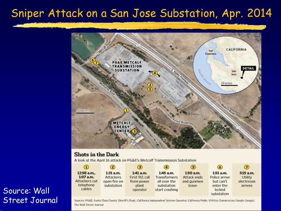
Sniper Attack on a San Jose Substation, Apr. 2014

Source: Wall Street Journal

Cascading Failures - Related Work

Report of the Commission to Assess the threat to the United States from Electromagnetic Pulse (EMP) Attack, 2008

Federal Energy Regulation Commission, Department of Energy, and Department of Homeland Security, Detailed Technical Report on EMP and Severe Solar Flare Threats to the U.S. Power Grid, Oct. 2010

Cascading failures in the power grid Dobson et al. (2001-2010), Hines et al. (2007-2010),

Chassin and Posse (2005), Gao et al. (2011),…

The N-k problem where the objective is to find the k links whose failures will cause the maximum damage: Bienstock et al. (2005, 2009)

Interdiction problems: Bier et al. (2007), Salmeron et al. (2009), …

Cascade control: Pfitzner et al. (2011), …

Mostly do not consider computational aspects

Outline

Background

Power flows and cascading failures

Real events, models, and simulations

Impact of single line failures

Pseudo-inverse of the admittance matrix and

resistance distance

Efficient algorithm for cascade evolution

Vulnerability analysis

Power Grid Vulnerability and Cascading Failures

Power flow follows the laws of physics

Control is difficult

It is difficult to “store packets” or “drop packets”

Modeling is difficult

Final report of the 2003 blackout – cause #1 was

“inadequate system understanding”

(stated at least 20 times)

Power grids are subject to cascading failures:

Initial failure event

Transmission lines fail due to overloads

Resulting in subsequent failures

Recent Major Blackout Event: San Diego, Sept. 2011

Blackout description (source: California Public Utility Commission)with the model

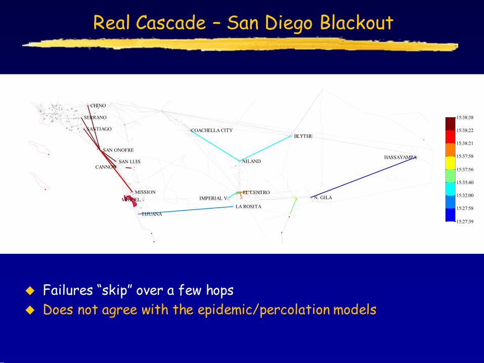
Real Cascade – San Diego Blackout

2100 2200 2300 2400 2500 2600 27001100

1150

1200

1250

1300

1350

HASSAYAMPA

N. GILA

LA ROSITA

TIJUANA

IMPERIAL V. MIGUEL

EL CENTRO

NILAND

BLYTHE

SAN ONOFRE

CANNON SAN LUIS

MISSION

SANTIAGO

SERRANO

CHINO

COACHELLA CITY

15:27:39

15:27:58

15:32:00

15:35:40

15:37:56

15:37:58

15:38:21

15:38:22

15:38:38

Failures “skip” over a few hops

Does not agree with the epidemic/percolation models

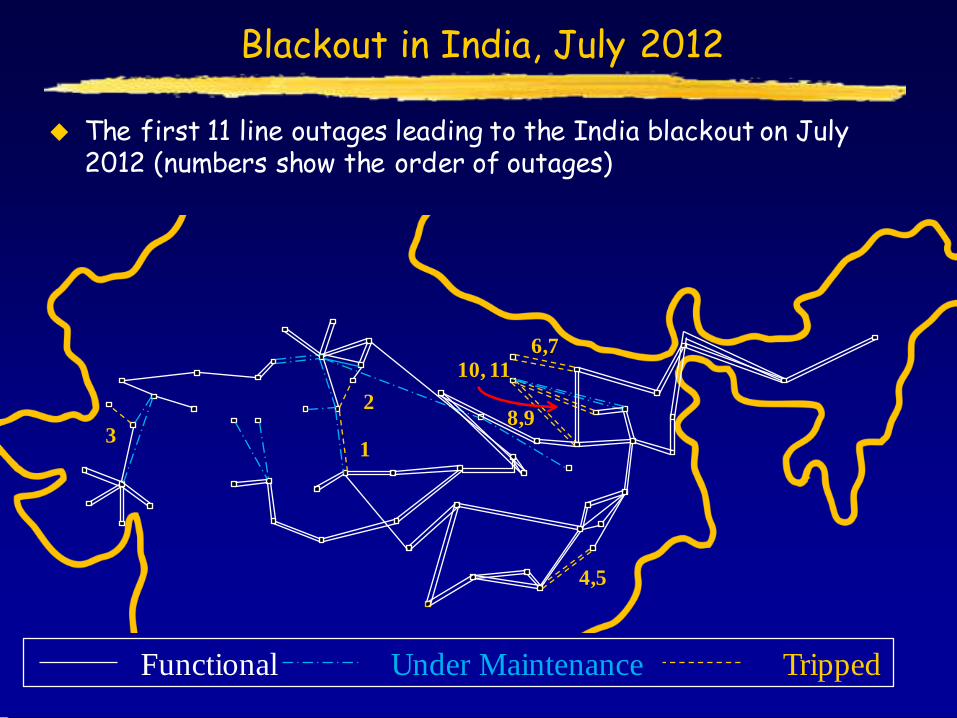
Blackout in India, July 2012

1

2

3

4,5

6,7

8,9

10, 11

Functional Under Maintenance Tripped

The first 11 line outages leading to the India blackout on July 2012 (numbers show the order of outages)

Power Flow Equations - DC Approximation

Exact solution to the AC model is infeasible

𝑓𝑖𝑗 = 𝑈𝑖2𝑔𝑖𝑗 − 𝑈𝑖𝑈𝑗𝑔𝑖𝑗 cos 𝜃𝑖𝑗 − 𝑈𝑖𝑈𝑗𝑏𝑖𝑗 sin 𝜃𝑖𝑗

𝑄𝑖𝑗 = −𝑈𝑖2𝑏𝑖𝑗 + 𝑈𝑖𝑈𝑗𝑏𝑖𝑗 cos𝜃𝑖𝑗 − 𝑈𝑖𝑈𝑗𝑔𝑖𝑗 sin 𝜃𝑖𝑗

and 𝜃𝑖𝑗 = 𝜃𝑖 − 𝜃𝑗 .

We use DC approximation which is based on:

𝑈𝑖 = 1 𝑝.𝑢. for all 𝑖

Pure reactive transmission lines – each line is characterized only by its reactance 𝑥𝑖𝑗 = −1/𝑏𝑖𝑗

Phase angle differences are “small”, implying that sin𝜃𝑖𝑗 ≈ 𝜃𝑖𝑗

Known as a reasonably good approximation

Frequently used for contingency analysis Do the assumptions hold during a cascade?

𝑗 𝑈𝑖 ≡ 1, ∀𝑖 𝑥𝑖𝑗

sin 𝜃𝑖𝑗 ≈ 𝜃𝑖𝑗

𝑖

𝑗

Load

Generator

𝑈𝑖, 𝜃𝑖, 𝑃𝑖, 𝑄𝑖

Power Flow Equations - DC Approximation

A power flow is a solution (𝑓,𝜃) of:

𝑓𝑢𝑣 = 𝑝𝑢

𝑣∈𝑁 𝑢

, ∀ 𝑢 ∈ 𝑉

𝜃𝑢 − 𝜃𝑣 − 𝑥𝑢𝑣𝑓𝑢𝑣 = 0,∀ 𝑢,𝑣 ∈ 𝐸

Matrix form: 𝐴Θ = 𝑃

𝐴 is the admittance matrix of the grid defined as:

𝑎𝑢𝑣 =

0, 𝑢 ≠ 𝑣 𝑎𝑛𝑑 𝑢, 𝑣 ∉ 𝐸

−1

𝑥𝑢𝑣, 𝑢 ≠ 𝑣 𝑎𝑛𝑑 𝑢, 𝑣 ∉ 𝐸

− 𝑎𝑣𝑤

𝑤∈𝑁 𝑢

, 𝑢 = 𝑣

If 𝐴+ is its pseudo-inverse Θ = 𝐴+𝑃

𝑢

𝑣

Load (𝑝𝑢 < 0)

Generator (𝑝𝑢 > 0)

𝜃𝑢,𝑝𝑢

Line Outage Rule

Different factors can be considered in modeling outage rules The main is thermal capacity 𝑢𝑖𝑗

Simplistic approach: fail lines with 𝑓𝑖𝑗 > 𝑢𝑖𝑗

Not part of the power flow problem constraints More realistic policy:

Compute the moving average 𝑓 𝑖𝑗 ≔ 𝛼 𝑓𝑖𝑗 + 1− 𝛼 𝑓 𝑖𝑗 (0 ≤ 𝛼 ≤ 1 is a parameter)

Deterministic outage rule: Fail lines with 𝑓 𝑖𝑗 > 𝑢𝑖𝑗

Stochastic outage rules

0

5

10

15

20

1 2 3 4 5 6

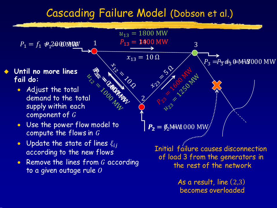
Cascading Failure Model (Dobson et al.)

𝑃1 = 𝑓1 = 2000 MW

𝑃2 = 𝑓2 = 1000 MW

𝑃13 = 1400 MW

𝑃3 = −𝑑3 = −3000 MW 𝑥13 = 10 Ω

1 3

2

𝑢13 = 1800 MW

𝑃13 = 3000 MW

𝑃3 = 0 MW

𝑃1 = 0 MW

𝑃2 = 0 MW

Until no more lines fail do:

Adjust the total demand to the total supply within each component of 𝐺

Use the power flow model to compute the flows in 𝐺

Update the state of lines 𝜉𝑖𝑗 according to the new flows

Remove the lines from 𝐺 according to a given outage rule 𝑂

Initial failure causes disconnection of load 3 from the generators in

the rest of the network

As a result, line 2,3 becomes overloaded

Numerical Results (Bernstein et al., IEEE INFOCOM’14)

Obtained from the GIS (Platts Geographic Information System)

Substantial processing of the raw data

Used a modified Western Interconnect system, to avoid exposing the vulnerability of the real grid

13,992 nodes (substations), 18,681 lines, and 1,920 power stations.

1,117 generators (red), 5,591 loads (green)

Assumed that demand is proportional to the population size

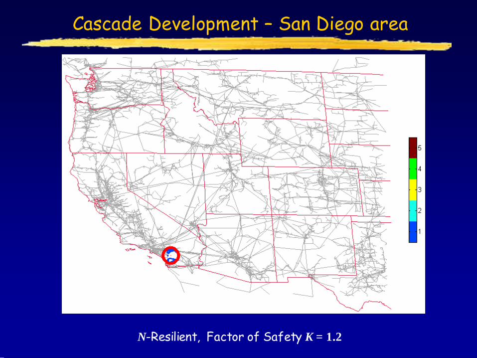
Cascade Development – San Diego area

N-Resilient, Factor of Safety K = 1.2

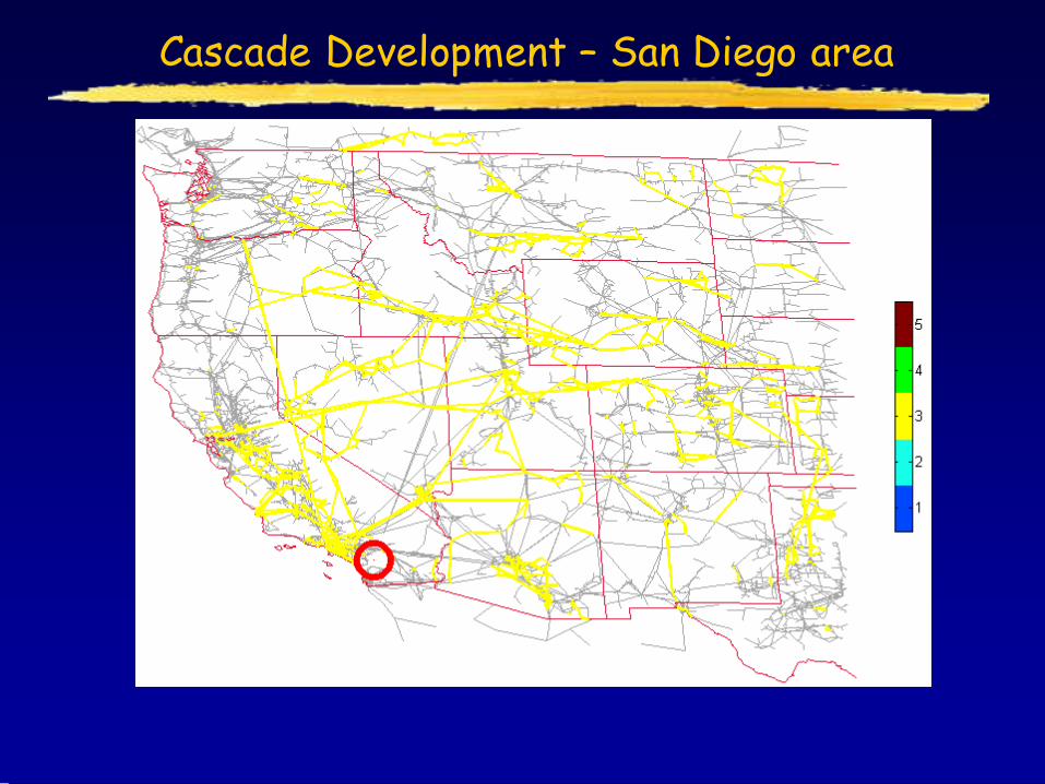
Cascade Development – San Diego area

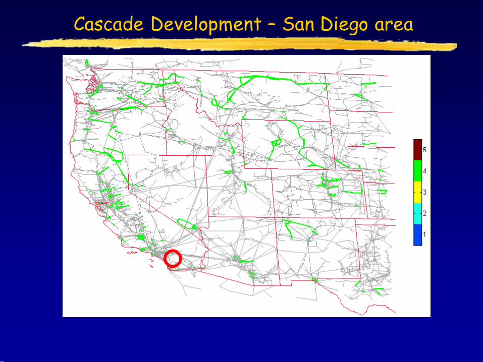
Cascade Development – San Diego area

Cascade Development – San Diego area

Cascade Development – San Diego area

Cascade Development – San Diego area

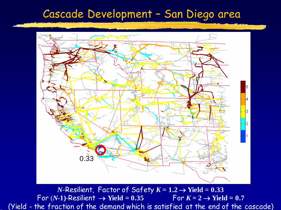
0.33

N-Resilient, Factor of Safety K = 1.2 Yield = 0.33

For (N-1)-Resilient Yield = 0.35 For K = 2 Yield = 0.7

(Yield - the fraction of the demand which is satisfied at the end of the cascade)

Outline

Background

Power flows and cascading failures

Real events, models, and simulations

Impact of single line failures

Pseudo-inverse of the admittance matrix and

resistance distance

Efficient algorithm for cascade evolution

Vulnerability analysis

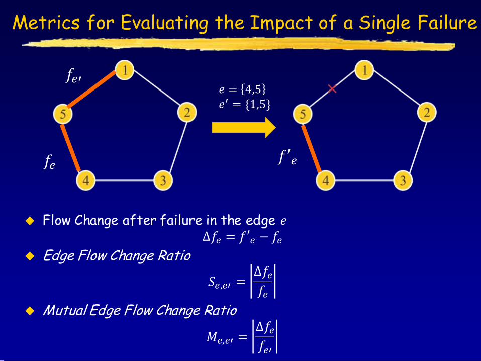
Metrics for Evaluating the Impact of a Single Failure

Flow Change after failure in the edge 𝑒 Δ𝑓𝑒 = 𝑓′𝑒 − 𝑓𝑒

Edge Flow Change Ratio

𝑆𝑒,𝑒′ =Δ𝑓𝑒

𝑓𝑒

Mutual Edge Flow Change Ratio

𝑀𝑒,𝑒′ =Δ𝑓𝑒

𝑓𝑒′

𝑒 = 4,5 𝑒′ = {1,5}

𝑓𝑒

𝑓𝑒′

𝑓′𝑒

Graph Used in Simulations

Western interconnection: 1708-edge connected subgraph of the U.S. Western interconnection

Erdos-Renyi graph: A random graph where each edge appears with probability 𝑝 = 0.01

Watts and Strogatz graph: A small-world random graph where each node connects to 𝑘 = 4 other nodes and the probability of rewiring is 𝑝 = 0.1

Barabasi and Albert graph: A scale-free random graph where each new node connects to 𝑘 = 3 other nodes at each step following the preferential attachment mechanism

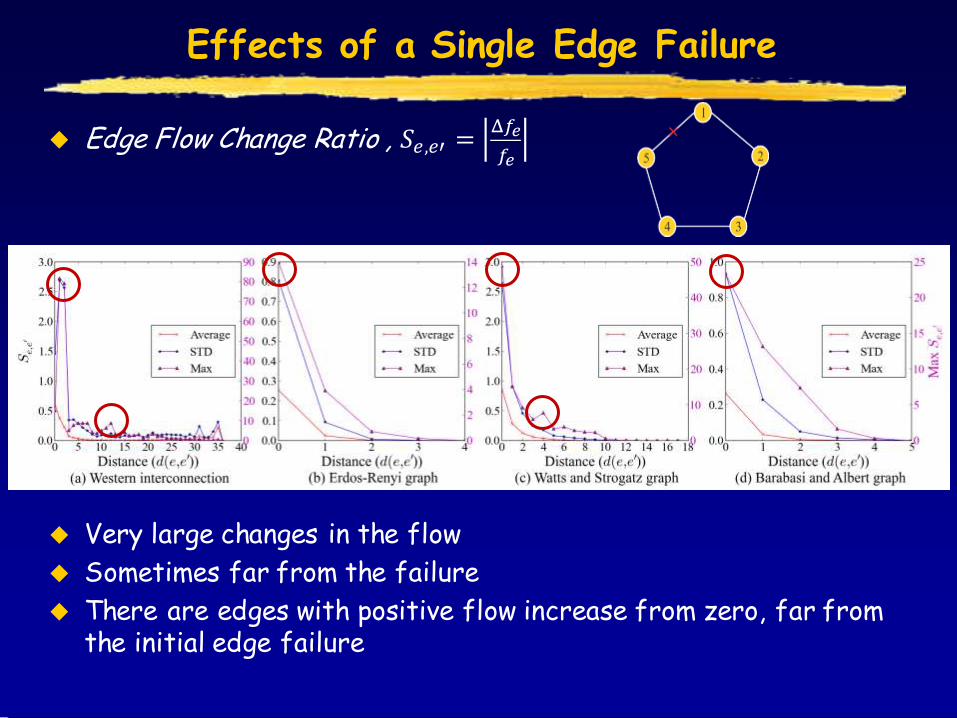
Effects of a Single Edge Failure

Edge Flow Change Ratio , 𝑆𝑒,𝑒′ =Δ𝑓𝑒

𝑓𝑒

Very large changes in the flow

Sometimes far from the failure

There are edges with positive flow increase from zero, far from the initial edge failure

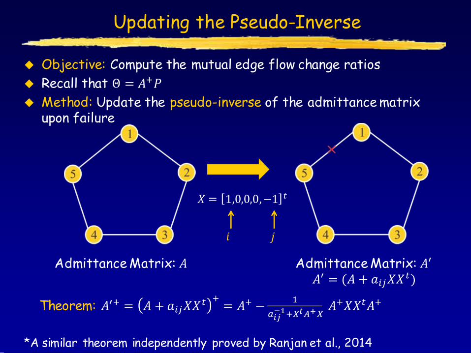
Objective: Compute the mutual edge flow change ratios

Recall that Θ = 𝐴+𝑃

Method: Update the pseudo-inverse of the admittance matrix upon failure

*A similar theorem independently proved by Ranjan et al., 2014

Updating the Pseudo-Inverse

Admittance Matrix: 𝐴 Admittance Matrix: 𝐴′ 𝐴′ = (𝐴 + 𝑎𝑖𝑗𝑋𝑋𝑡)

𝑋 = 1,0,0,0,−1 𝑡

𝑖 𝑗

Theorem: 𝐴′+ = 𝐴 + 𝑎𝑖𝑗𝑋𝑋𝑡 += 𝐴+ −

1

𝑎𝑖𝑗−1+𝑋𝑡𝐴+𝑋

𝐴+𝑋𝑋𝑡𝐴+

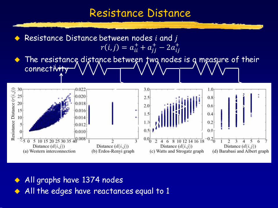
Resistance Distance

Resistance Distance between nodes 𝑖 and 𝑗 𝑟 𝑖, 𝑗 = 𝑎𝑖𝑖

+ + 𝑎𝑗𝑗+ − 2𝑎𝑖𝑗

+

The resistance distance between two nodes is a measure of their connectivity

All graphs have 1374 nodes

All the edges have reactances equal to 1

𝑟 𝑖, 𝑗

𝑗

𝑖

Effects of a Single Edge Failure

Mutual Edge Flow Change Ratio

𝑀𝑒,𝑒′ =Δ𝑓𝑒

𝑓𝑒′

Using pseudo-inverse of the admittance matrix, 𝑒 = 𝑖, 𝑗 , 𝑒′ = {𝑝,𝑞}

𝑀𝑒,𝑒′ =1

2

−𝑟 𝑖,𝑝 + 𝑟 𝑖, 𝑞 + 𝑟 𝑗, 𝑝 − 𝑟(𝑗, 𝑞)

1 − 𝑟 𝑝, 𝑞

Mutual Edge flow change ratios (𝑀𝑒,𝑒′) are independent of the supply and demand

Initial Failure Represented by a black wide line

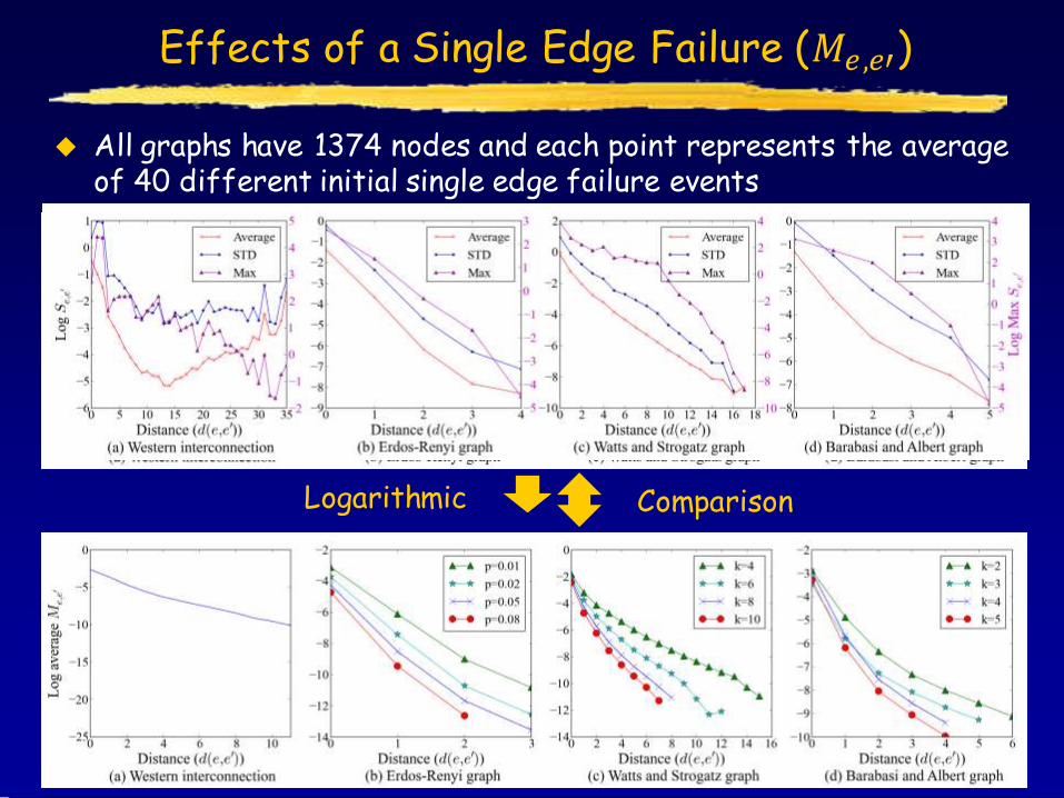
Effects of a Single Edge Failure (𝑀𝑒,𝑒′)

Logarithmic

All graphs have 1374 nodes and each point represents the average of 40 different initial single edge failure events

Comparison

Efficient Cascading Failure Evolution Computation

𝐴 =

2 −1 0 0 0−1 2 −1 0 00 −1 2 −1 00 0 −1 2 −1

−1 0 0 −1 2

𝐴+ =

0.4 0 −0.2 −0.2 00 0.4 0 −0.2 −0.2

−0.2 0 0.4 0 −0.2−0.2 −0.2 0 0.4 0

0 −0.2 −0.2 0 0.4

𝐴′ =

1 −1 0 0 0−1 2 −1 0 00 −1 2 −1 00 0 −1 2 −10 0 0 −1 1

𝐴′+ =

1.2 0.4 −0.2 −0.6 −0.80.4 0.6 0 −0.4 −0.6

−0.2 0 0.4 0 −0.2−0.6 −0.4 0 0.6 0.4−0.8 −0.6 −0.2 0.4 .2

• Case I: Failure of an edge

which is not a cut-edge

Update 𝐴+ after

removing the edge

{1,5}, in 𝑂( 𝑉 2)

Efficient Cascading Failure Evolution Computation

𝐴′ =

1 −1 0 0 0−1 2 −1 0 00 −1 2 −1 00 0 −1 2 −10 0 0 −1 1

𝐴′+ =

1.2 0.4 −0.2 −0.6 −0.80.4 0.6 0 −0.4 −0.6

−0.2 0 0.4 0 −0.2−0.6 −0.4 0 0.6 0.4−0.8 −0.6 −0.2 0.4 .2

Detect the cut-edge and

connected components in

𝑂 𝑉

Adjust the total demand to

equal the total supply within

each connected component

No need to update 𝐴+

• Case II: Failure of a

cut-edge

𝐴′′ =

1 −1 0 0 0−1 1 0 0 00 0 1 −1 00 0 −1 2 −10 0 0 −1 1

𝑎′23−1 − 2𝑎′23

+ + 𝑎′22+ + 𝑎′33

+ = 0

𝐴2′+ − 𝐴3

′+ = 0.6 0.6 −0.4 −0.4 −0.4

𝐺1 𝐺2

𝐺1

𝐺2

Efficient Cascading Failure Evolution Computation

The Pseudo-inverse Based Algorithm identifies the evolution of

the cascade in 𝑂( 𝑉 3 + 𝐹𝑡∗ 𝑉 2)

Compared to the classical algorithm which runs in 𝑂(𝑡 𝑉 3)

If 𝑡 = |𝐹𝑡∗| (one edge fails at each round), our algorithm performs

𝑂(min {|𝑉|, 𝑡}) faster

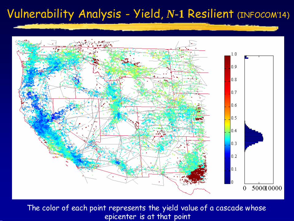
Vulnerability Analysis - Yield, N-1 Resilient (INFOCOM’14)

The color of each point represents the yield value of a cascade whose epicenter is at that point

Heuristic Algorithm for Min Yield Problem

Yield: The ratio between the demand supplied at stabilization and its original value

The minimum Yield problem is NP-hard

Based on our results, after failure on an edge {𝑝, 𝑞}, the flow

changes can be bounded by Δ𝑓𝑖𝑗 ≤𝑟 𝑝,𝑞

1−𝑟 𝑝,𝑞 𝑓𝑝𝑞

Edges with large 𝑟 𝑝,𝑞 𝑓𝑝𝑞 have large impact on flow changes

The algorithm removes edges with large 𝑟 𝑝, 𝑞 𝑓𝑝𝑞

The yield at stabilization

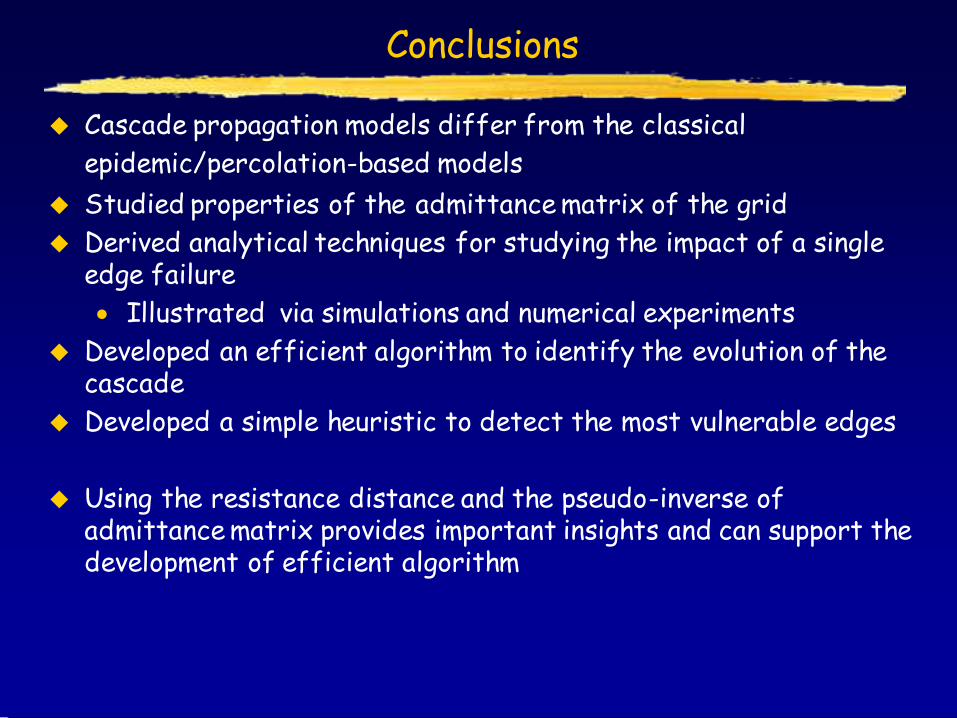
Conclusions

Cascade propagation models differ from the classical

epidemic/percolation-based models

Studied properties of the admittance matrix of the grid

Derived analytical techniques for studying the impact of a single edge failure

Illustrated via simulations and numerical experiments

Developed an efficient algorithm to identify the evolution of the cascade

Developed a simple heuristic to detect the most vulnerable edges

Using the resistance distance and the pseudo-inverse of admittance matrix provides important insights and can support the development of efficient algorithm