sample average approximation and cascading failures … · sample average approximation and...
TRANSCRIPT

Sample average approximation and cascadingfailures of power grids
Daniel Bienstock, Guy Grebla, Tingjun Chen, Columbia UniversityGraphEx ’15
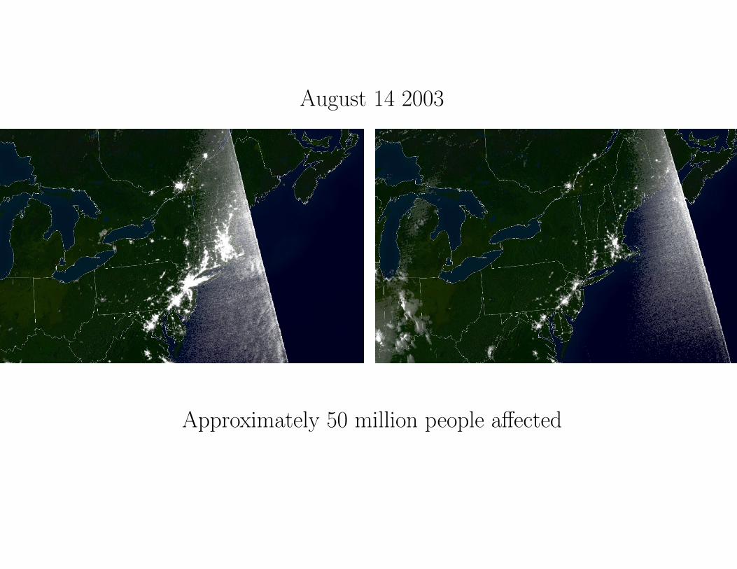
August 14 2003
Approximately 50 million people affected

Other large-scale cascading failures
• Italy, 2003
• San Diego, 2011
• India, 2012
At fault:
unexpected event, cascading mechanism, noise and human error

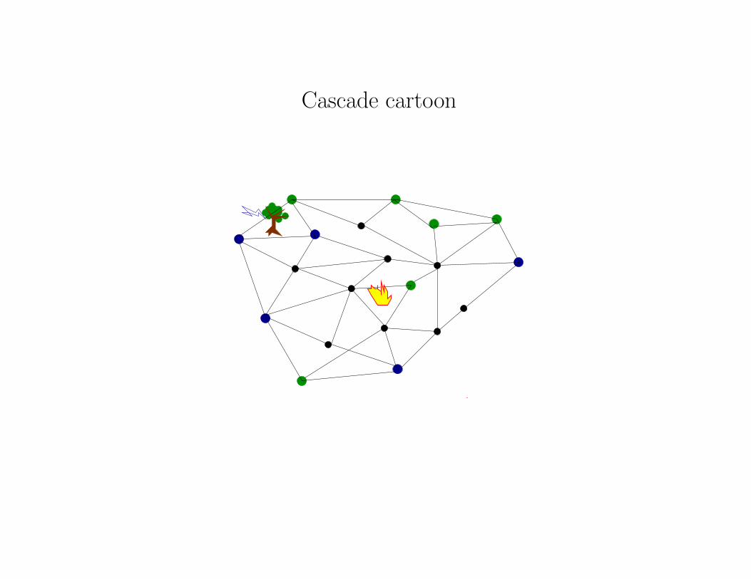
Cascade cartoon
Generator
Load (demand)
Cascade cartoon
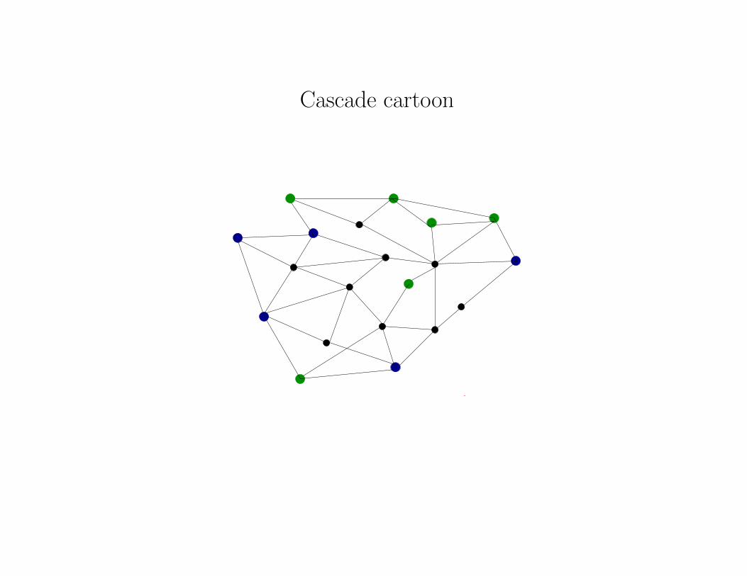
Cascade cartoon

Cascade cartoon
Cascade cartoon

Cascade cartoon
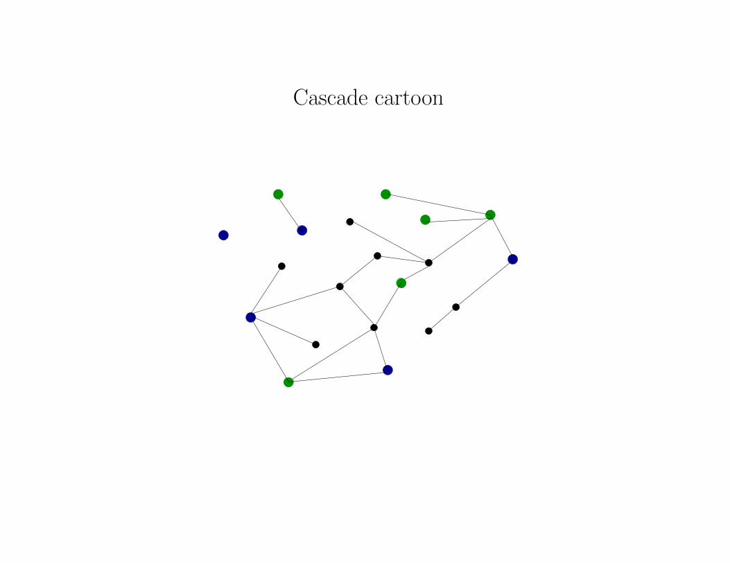
= lost demand

Cascade cartoon

Cascade cartoon
A quote from:
Final Report on the August 14, 2003 Blackout in the UnitedStates and Canada: Causes and Recommendations,
(U.S.-Canada Power System Outage Task Force)
Cause 1 of the blackout was “inadequate system understanding”
A quote from:
Final Report on the August 14, 2003 Blackout in the UnitedStates and Canada: Causes and Recommendations,
(U.S.-Canada Power System Outage Task Force)
Cause 1 of the blackout was “inadequate system understanding”
(stated at least twenty times)

A quote from:
Final Report on the August 14, 2003 Blackout in the UnitedStates and Canada: Causes and Recommendations,
(U.S.-Canada Power System Outage Task Force)
Cause 1 of the blackout was “inadequate system understanding”
(stated at least twenty times)
Cause 2 of the blackout was “inadequate situational awareness”

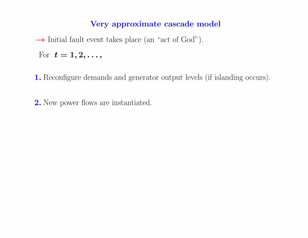
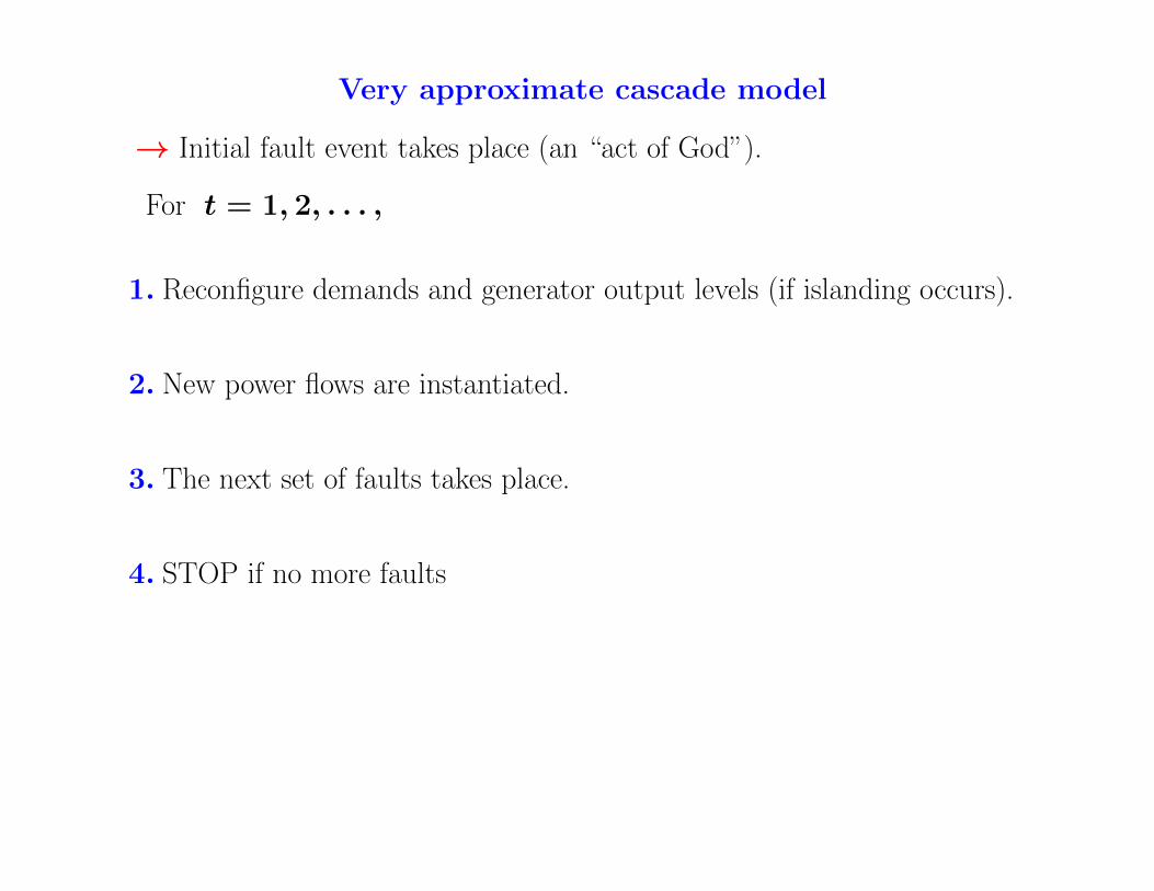
Very approximate cascade model
→ Initial fault event takes place (an “act of God”).
For t = 1, 2, . . . ,
1. Reconfigure demands and generator output levels (if islanding occurs).

Islanding
supply > demand

The “swing” equation
• A second-order differential equation used to explain swings in a motor’sfrequency in response to a change of loads.
• To properly analyize islanding, we need to consider systems of swing equa-tions, plus physics of power flows.
•Which is a very difficult computational problem.
• Primary, secondary frequency response.
Very approximate cascade model
→ Initial fault event takes place (an “act of God”).
For t = 1, 2, . . . ,
1. Reconfigure demands and generator output levels (if islanding occurs).
2. New power flows are instantiated.

Power flow problem in rectangular coordinates, simplest form
Variables: Complex voltages ek + jfk, power flows Pkm, Qkm
Notation: For a bus k, δ(k) = set of lines incident with k;V = set of buses
∀km : Pkm = gkm(e2k + f 2k )− gkm(ekem + fkfm) + bkm(ekfm − fkem) (1a)
∀km : Qkm = −bkm(e2k + f 2k ) + bkm(ekem + fkfm) + gkm(ekfm − fkem) (1b)
∀km : |Pkm|2 + |Qkm|2 ≤ Ukm (1c)
∀k : Pmink ≤
∑km∈ δ(k)
Pkm ≤ Pmaxk (1d)
∀k : Qmink ≤
∑km∈ δ(k)
Qkm ≤ Qmaxk (1e)
∀k : V mink ≤ e2k + f 2k ≤ V max
k . (1f)
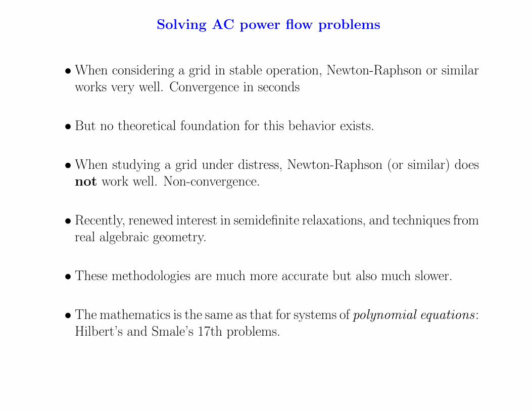
Solving AC power flow problems
•When considering a grid in stable operation, Newton-Raphson or similarworks very well. Convergence in seconds
• But no theoretical foundation for this behavior exists.
•When studying a grid under distress, Newton-Raphson (or similar) doesnot work well. Non-convergence.
• Recently, renewed interest in semidefinite relaxations, and techniques fromreal algebraic geometry.
• These methodologies are much more accurate but also much slower.
• The mathematics is the same as that for systems of polynomial equations :Hilbert’s and Smale’s 17th problems.

Very approximate cascade model
→ Initial fault event takes place (an “act of God”).
For t = 1, 2, . . . ,
1. Reconfigure demands and generator output levels (if islanding occurs).
2. New power flows are instantiated.
3. The next set of faults takes place.

Line tripping
1. If a power line carries too much power, it will overheat.
2. At a critical temperature, the line will fail.
3. Before that point, the line will sag. A physical contact would lead toimmeadite tripping.
4. If a line is overloaded for too long, it will be protectively tripped.
5. Simplification: there is a line limit beyond which a line is consideredoverloaded.
5. IEEE Standard 738. An adaptation of the heat equation so as to takeinto account ...

Line tripping
1. If a power line carries too much power, it will overheat.
2. At a critical temperature, the line will fail.
3. Before that point, the line will sag. A physical contact would lead toimmeadite tripping.
4. If a line is overloaded for too long, it will be protectively tripped.
5. Simplification: there is a line limit beyond which a line is consideredoverloaded.
5. IEEE Standard 738. An adaptation of the heat equation so as to takeinto account ... the state of the universe, pretty much
(current work: appropriate stochastic variants of the heat equation)
Very approximate cascade model
→ Initial fault event takes place (an “act of God”).
For t = 1, 2, . . . ,
1. Reconfigure demands and generator output levels (if islanding occurs).
2. New power flows are instantiated.
3. The next set of faults takes place.
4. STOP if no more faults
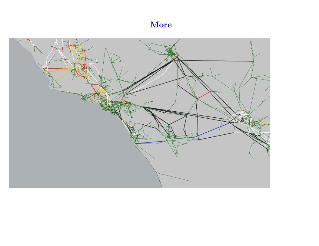
Simulation of 2011 San Diego Event
Joint work with A. Bernstein, D. Hay, G. Zussman, M. Uzunoglu(EE Dept. Columbia)
• Initiating event: human error
•We do not have complete or exact data
•Nevertheless, in our simulations a cascade does take place,with similar characteristics at the initial stages
• “inadequate system understanding”
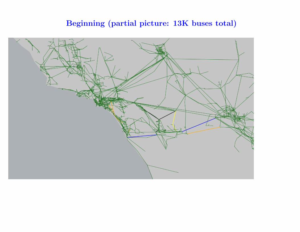
Beginning (partial picture: 13K buses total)

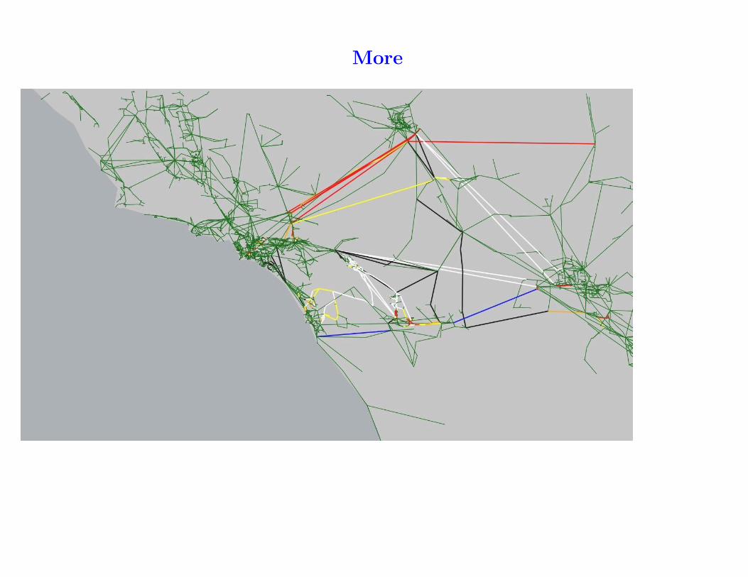
More
More
More

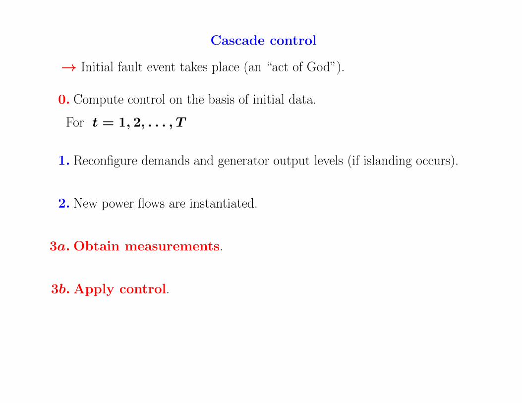
Cascade control
→ Initial fault event takes place (an “act of God”).
0. Compute control on the basis of initial data.

Cascade control
→ Initial fault event takes place (an “act of God”).
0. Compute control on the basis of initial data.
For t = 1, 2, . . . , T
1. Reconfigure demands and generator output levels (if islanding occurs).
2. New power flows are instantiated.

Cascade control
→ Initial fault event takes place (an “act of God”).
0. Compute control on the basis of initial data.
For t = 1, 2, . . . , T
1. Reconfigure demands and generator output levels (if islanding occurs).
2. New power flows are instantiated.
3a.Obtain measurements.
Cascade control
→ Initial fault event takes place (an “act of God”).
0. Compute control on the basis of initial data.
For t = 1, 2, . . . , T
1. Reconfigure demands and generator output levels (if islanding occurs).
2. New power flows are instantiated.
3a.Obtain measurements.
3b.Apply control.

Cascade control
→ Initial fault event takes place (an “act of God”).
0. Compute control on the basis of initial data.
For t = 1, 2, . . . , T
1. Reconfigure demands and generator output levels (if islanding occurs).
2. New power flows are instantiated.
3a.Obtain measurements.
3b.Apply control.
3. The next set of faults takes place.
4. If t = T proportionally shed enough load to stop cascade.

A basic form of affine control
• Control consists of nonnegative parameters u1, u2, . . . , uT .
• At time t, on an island C with max line overload κC, scale demandsby
1 + ut (1 − κC)
• κC > 1 implies loss of demand
• Easy to apply?

Clairvoyant control
• For any island C that exists at time t, a parameter ut,C.
• At time t, on island C with max line overload κC, scale demands by
1 + ut,C (1 − κC)
• κC > 1 implies loss of demand
• Easy to apply? Does it even make sense?

A basic form of affine control
• Control consists of nonnegative parameters u1, u2, . . . , uT .
• At time t, on an island C with max line overload κC, scale demandsby
1 + ut (1 − κC)
• κC > 1 implies loss of demand
• Easy to apply?

An even simpler form of affine control
• Control consists of nonnegative parameters λ1, λ2, . . . , λT .
• At time t, all demands scaled by λt
• Easy to apply.
• But conservative?
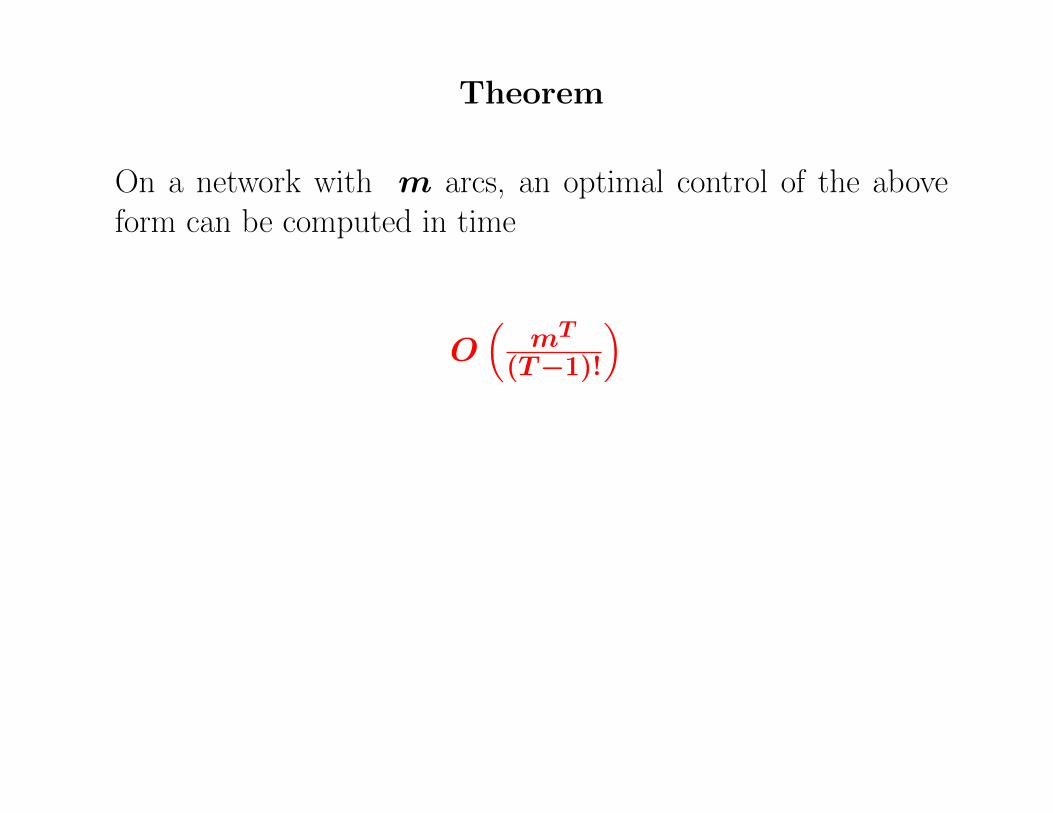
Theorem
On a network with m arcs, an optimal control of the aboveform can be computed in time
O(
mT
(T−1)!
)

Theorem
On a network with m arcs, an optimal control of the aboveform can be computed in time
O(
mT
(T−1)!
)
→ What is the mathematics to explain “games” of this sort?

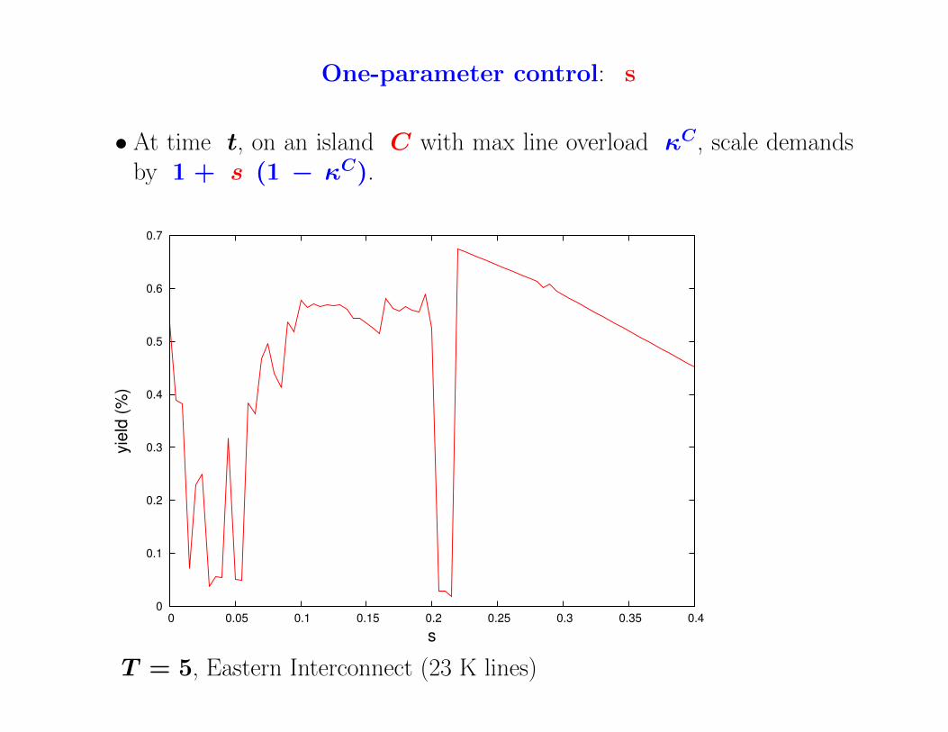
One-parameter control: s
• At time t, on an island C with max line overload κC, scale demandsby 1 + s (1 − κC).
One-parameter control: s
• At time t, on an island C with max line overload κC, scale demandsby 1 + s (1 − κC).
0
0.1
0.2
0.3
0.4
0.5
0.6
0.7
0 0.05 0.1 0.15 0.2 0.25 0.3 0.35 0.4
yie
ld (
%)
s
T = 5, Eastern Interconnect (23 K lines)
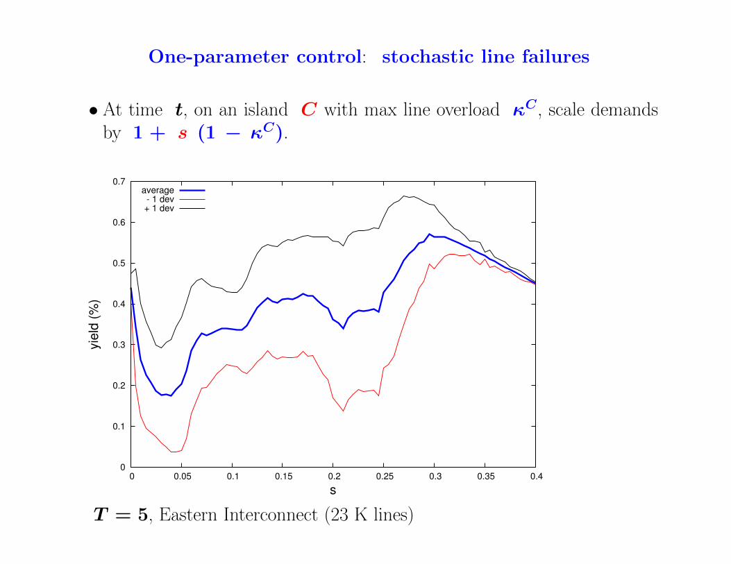
One-parameter control: stochastic line failures
• At time t, on an island C with max line overload κC, scale demandsby 1 + s (1 − κC).
0
0.1
0.2
0.3
0.4
0.5
0.6
0.7
0 0.05 0.1 0.15 0.2 0.25 0.3 0.35 0.4
yie
ld (
%)
s
average- 1 dev+ 1 dev
T = 5, Eastern Interconnect (23 K lines)

Robustness through noise: the sample average approach
• Let L̂j be the limit of line j, j = 1, . . . ,m (= number of lines).
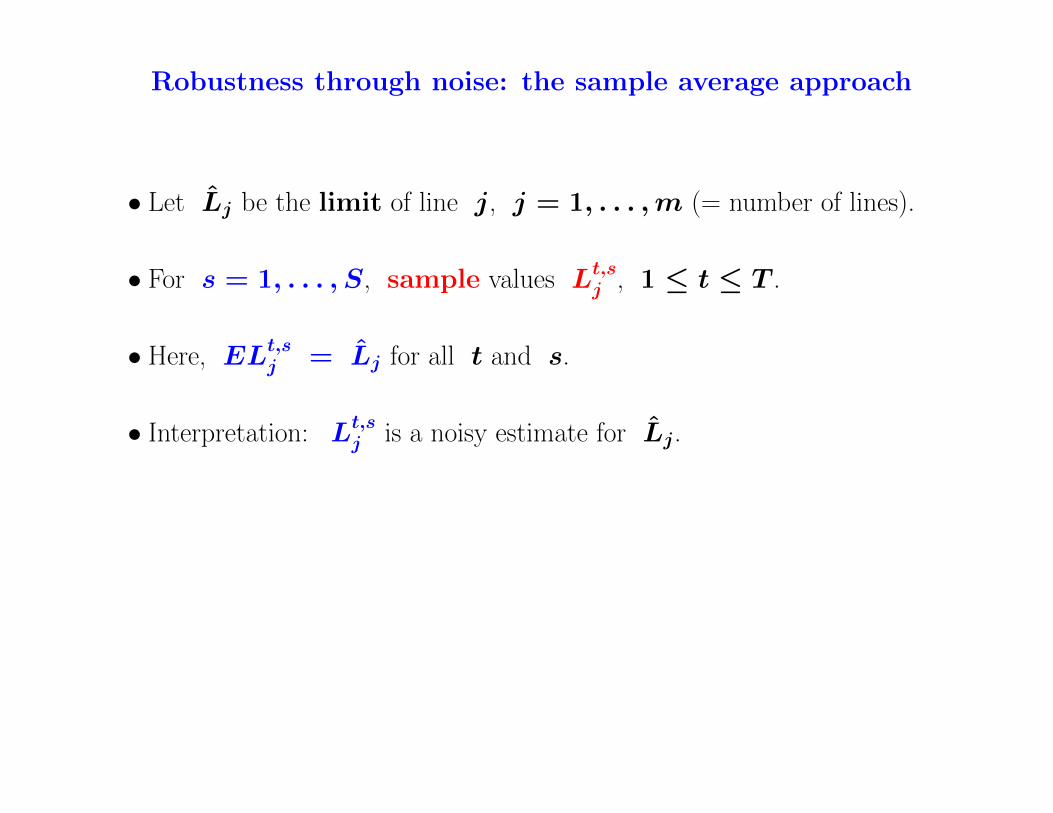
Robustness through noise: the sample average approach
• Let L̂j be the limit of line j, j = 1, . . . ,m (= number of lines).
• For s = 1, . . . , S, sample values Lt,sj , 1 ≤ t ≤ T .
• Here, ELt,sj = L̂j for all t and s.
• Interpretation: Lt,sj is a noisy estimate for L̂j.
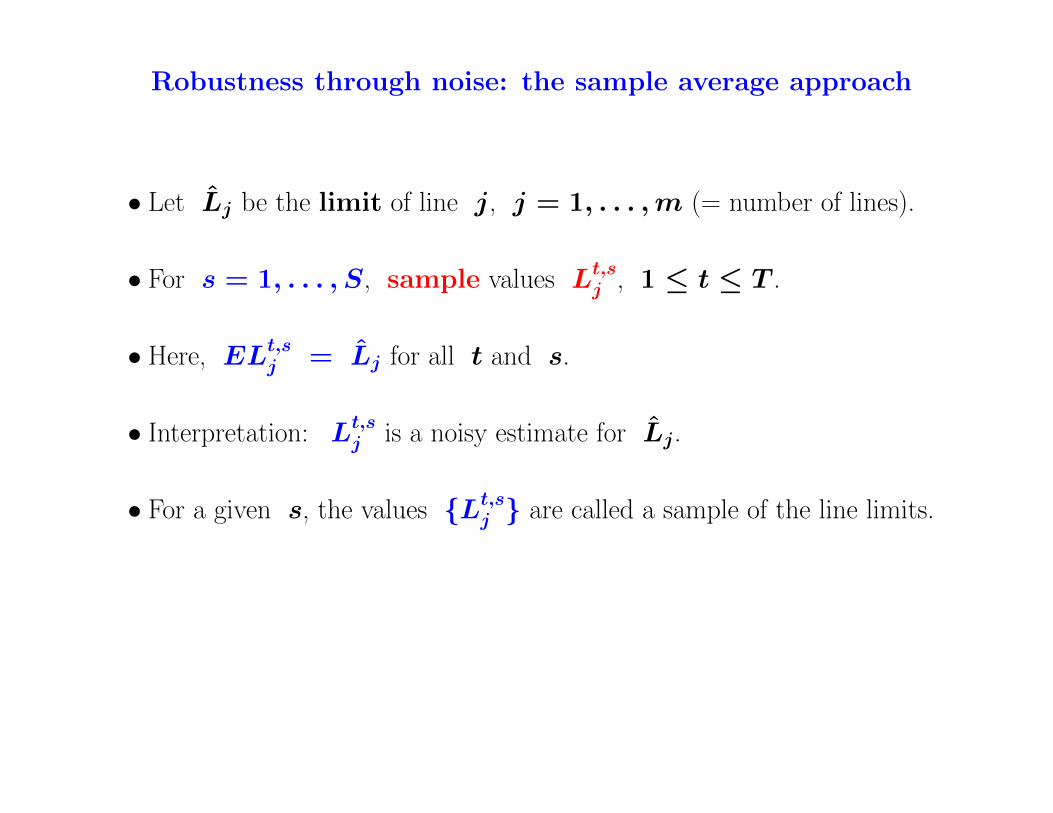
Robustness through noise: the sample average approach
• Let L̂j be the limit of line j, j = 1, . . . ,m (= number of lines).
• For s = 1, . . . , S, sample values Lt,sj , 1 ≤ t ≤ T .
• Here, ELt,sj = L̂j for all t and s.
• Interpretation: Lt,sj is a noisy estimate for L̂j.
• For a given s, the values {Lt,sj } are called a sample of the line limits.
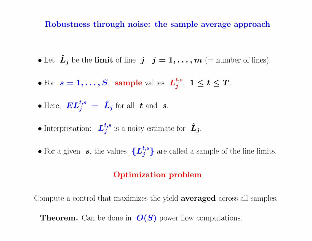
Optimization problem
Compute a control that maximizes the yield averaged across all samples.
Theorem. Can be done in O(S) power flow computations.
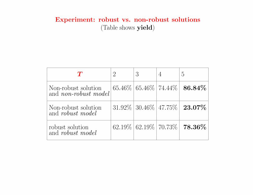
Experiment: robust vs. non-robust solutions(Table shows yield)
T 2 3 4 5
Non-robust solution 65.46% 65.46% 74.44% 86.84%and non-robust model
Non-robust solution 31.92% 30.46% 47.75% 23.07%and robust model
robust solution 62.19% 62.19% 70.73% 78.36%and robust model