cascading failures in power grids – analysis and...
TRANSCRIPT
Cascading Failures in Power Grids –Analysis and Algorithms
Saleh SoltanElectrical EngineeringColumbia University
New York, [email protected]
Dorian MazauricLaboratoire d’InformatiqueFondamentale de Marseille
Marseille, [email protected]
Gil ZussmanElectrical EngineeringColumbia University
New York, [email protected]
ABSTRACTThis paper focuses on cascading line failures in the trans-mission system of the power grid. Recent large-scale poweroutages demonstrated the limitations of percolation- andepidemic-based tools in modeling cascades. Hence, we studycascades by using computational tools and a linearized powerflow model. We first obtain results regarding the Moore-Penrose pseudo-inverse of the power grid admittance matrix.Based on these results, we study the impact of a single linefailure on the flows on other lines. We also illustrate via sim-ulation the impact of the distance and resistance distance onthe flow increase following a failure, and discuss the differ-ence from the epidemic models. We use the pseudo-inverse ofadmittance matrix to develop an efficient algorithm to iden-tify the cascading failure evolution, which can be a buildingblock for cascade mitigation. Finally, we show that findingthe set of lines whose removal results in the minimum yield(the fraction of demand satisfied after the cascade) is NP-Hard and introduce a simple heuristic for finding such a set.Overall, the results demonstrate that using the resistancedistance and the pseudo-inverse of admittance matrix pro-vides important insights and can support the developmentof efficient algorithms.
Categories and Subject DescriptorsC.4 [Performance of Systems]: Reliability, availability,and serviceability; G.2.2 [Discrete Mathematics]: GraphTheory—Graph algorithms, Network problems
KeywordsPower Grid; Pseudo-inverse; Cascading Failures; Algorithms
Permission to make digital or hard copies of all or part of this work for personal orclassroom use is granted without fee provided that copies are not made or distributedfor profit or commercial advantage and that copies bear this notice and the full citationon the first page. Copyrights for components of this work owned by others than theauthor(s) must be honored. Abstracting with credit is permitted. To copy otherwise, orrepublish, to post on servers or to redistribute to lists, requires prior specific permissionand/or a fee. Request permissions from [email protected]’14, June 11–13, 2014, Cambridge, UK.Copyright is held by the owner/author(s). Publication rights licensed to ACM.ACM 978-1-4503-2819-7/14/067 ...$15.00.http://dx.doi.org/10.1145/2602044.2602066.
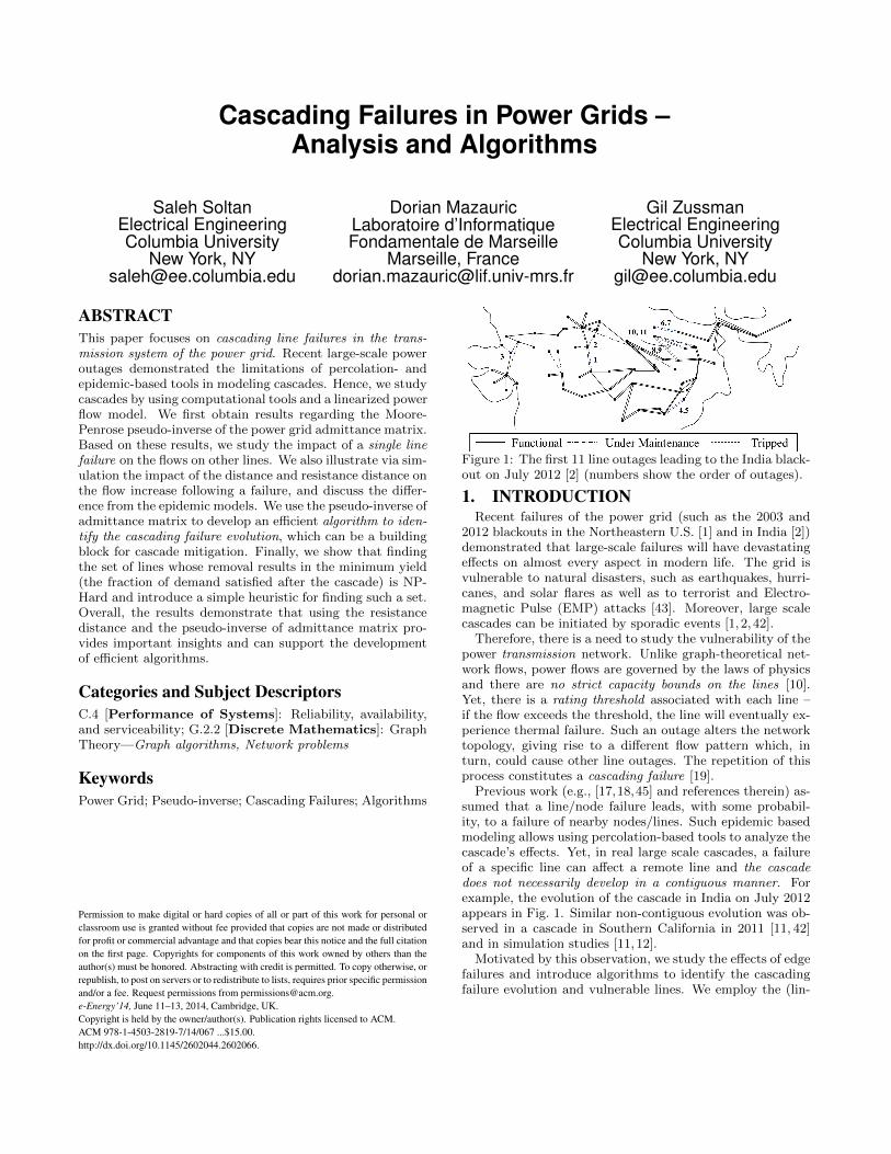
Figure 1: The first 11 line outages leading to the India black-out on July 2012 [2] (numbers show the order of outages).
1. INTRODUCTIONRecent failures of the power grid (such as the 2003 and
2012 blackouts in the Northeastern U.S. [1] and in India [2])demonstrated that large-scale failures will have devastatingeffects on almost every aspect in modern life. The grid isvulnerable to natural disasters, such as earthquakes, hurri-canes, and solar flares as well as to terrorist and Electro-magnetic Pulse (EMP) attacks [43]. Moreover, large scalecascades can be initiated by sporadic events [1, 2, 42].
Therefore, there is a need to study the vulnerability of thepower transmission network. Unlike graph-theoretical net-work flows, power flows are governed by the laws of physicsand there are no strict capacity bounds on the lines [10].Yet, there is a rating threshold associated with each line –if the flow exceeds the threshold, the line will eventually ex-perience thermal failure. Such an outage alters the networktopology, giving rise to a different flow pattern which, inturn, could cause other line outages. The repetition of thisprocess constitutes a cascading failure [19].
Previous work (e.g., [17,18,45] and references therein) as-sumed that a line/node failure leads, with some probabil-ity, to a failure of nearby nodes/lines. Such epidemic basedmodeling allows using percolation-based tools to analyze thecascade’s effects. Yet, in real large scale cascades, a failureof a specific line can affect a remote line and the cascadedoes not necessarily develop in a contiguous manner. Forexample, the evolution of the cascade in India on July 2012appears in Fig. 1. Similar non-contiguous evolution was ob-served in a cascade in Southern California in 2011 [11, 42]and in simulation studies [11,12].
Motivated by this observation, we study the effects of edgefailures and introduce algorithms to identify the cascadingfailure evolution and vulnerable lines. We employ the (lin-
earized) direct-current (DC) power flow model,1 which is apractical relaxation of the alternating-current (AC) model,and the cascading failure model of [25] (see also [11–14]).Specifically, we first review the model and the CascadingFailure Evolution (CFE) Algorithm that has been used toidentify the evolution of the cascade [13,14,19] (its complex-ity is O(t|V |3), where |V | is the number of nodes and t isthe number of cascade rounds).
Then, in order to investigate the impact of a single edgefailure on other edges, we use matrix analysis tools to studythe properties of the admittance matrix of the grid2 andMoore-Penrose Pseudo-inverse [4] of the admittance matrix.In particular, we provide a rank-1 update of the pseudo-inverse of the admittance matrix after a single edge failure.
We use these results along with the resistance distance andKirchhoff’s index notions3 to study the impact of a singleedge failure on the flows on other edges. We obtain upperbounds on the flow changes after a single failure and studythe robustness of specific graph classes. We also illustratevia simulations the relation between the flow changes aftera failure and the distance (in hop count) and resistance dis-tance from the failure in the U.S. Western interconnectionas well as Erdos-Renyi [26], Watts and Strogatz [44], andBarabasi and Albert [9] graphs. These simulations showthat there are cases in which an edge flow far away from thefailure significantly increases. These observations are clearlyin contrast to the epidemic-based models.
Once lines fail, there is a need for low complexity al-gorithms to control and mitigate the cascade. Hence, wedevelop the low complexity Cascading Failure Evolution –Pseudo-inverse Based (CFE-PB) Algorithm for identifyingthe evolution of a cascade that may be initiated by a fail-ure of several edges. The algorithm is based on the rank-1update of the pseudo-inverse of the admittance matrix. Weshow that its complexity is O(|V |3 + |F ∗t ||V |2) (|F ∗t | is thenumber of edges that eventually fail). Namely, if t = |F ∗t |(one edge fails at each round), the complexity of the CFE-PB Algorithm is O(min|V |, t) times lower than that of theCFE Algorithm. The main advantage of the CFE-PB Algo-rithm is that it leverages the special structure of the pseudo-inverse to identify properties of the underlying graph and torecompute an instance of the pseudo-inverse from a previousinstance.
Finally, we prove that the problem of finding the set ofinitial failures of size k that causes a cascade with the min-imum possible yield (the fraction of demand satisfied af-ter the cascade) is NP-hard. We introduce a very simpleheuristic termed the Most Vulnerable Edges Selection – Re-sistance distance Based (MVES-RB) Algorithm. We numer-ically show that solutions obtained by it lead to a much loweryield than the solutions obtain by selecting the initial edgefailures randomly. Moreover, in some small graphs with asingle edge failure, it obtains the optimal solution.
The main contribution of this paper is the development ofnew tools, based on matrix analysis, for assessing the impactof a single edge failure. Using these tools, we (i) obtain upperbounds on the flow changes after a single failure, (ii) develop
1The DC model is commonly used in large-scale contin-gency analysis of power grids [13,14,38].
2An n× n admittance matrix represents the admittanceof the lines in a power grid with n nodes.
3These notions originate from Circuit Theory and arewidely used in Chemistry [29].
a fast algorithm for identifying the evolution of the cascade,and (iii) develop a heuristic algorithm for the minimum yieldproblem.
This paper is organized as follows. Section 2 reviews re-lated work. Section 3 describes the power flow, cascademodel, metrics, and the graphs used in the simulations. InSection 4, we derive the properties of the admittance ma-trix of the grid. Section 5 presents the effects of a singleedge failure. Section 6 introduces the CFE-PB Algorithm.Section 7 discusses the hardness of the minimum yield prob-lem and introduces the MVES-RB Algorithm. Section 8provides concluding remarks and directions for future work.The proofs appear in the Appendix.
2. RELATED WORKNetwork vulnerability to attacks has been thoroughly stud-
ied (e.g., [3, 30, 37] and references therein). However, mostprevious computational work did not consider power gridsand cascading failures. Recent work on cascades focusedon probabilistic failure propagation models (e.g., [17,18,45],and references therein). However, real cascades [1,2,42] andsimulation studies [11, 12] indicate that the cascade propa-gation is different than that predicted by such models.
In Sections 4 and 6, we use the admittance matrix of thegrid to compute flows. This is tightly connected to the prob-lem of solving Laplacian systems. Solving these systems canbe done with several techniques, including Gaussian elim-ination and LU factorization [27]. Recently, [20] designedalgorithms that use preconditioning, to provide highly pre-cise approximate solutions to Laplacian systems in nearlylinear time. However, this approach only provides approx-imate solutions and is not suitable for analytical studies ofthe effects of edge failures.
In Section 5, we obtain upper bounds on the flow changesafter a single failure and study the robustness of graph classesbased on resistance distance and Kirchhoff’s index [16, 29].Recently, these notions have gained attention outside theChemistry community. For instance, they were used in net-work science for detecting communities within a network,and more generally the strength of the connection betweennodes in a network [34,35]. Moreover, [22] recently used theresistance distance to partition power systems into zones.
The problem of identifying the set of failures with thelargest impact was studied in [13, 14, 32, 38]. In particu-lar, [14] studies the N − k problem which focuses on find-ing a small cardinality set of links whose removal disablesthe network from delivering a minimum amount of demand.A broader network interdiction problem in which all thecomponents of the network are subject to failure was stud-ied in [41]. A similar problem is studied in [38] using thealternating-current (AC) model. However, none of the pre-vious works consider the cascading failures. Moreover, whilethe optimal power flow problem has been shown to be NP-hard [31], the complexity of the cascade-related problemswas not studied yet.
Finally, for the simulations, we use graphs that can rep-resent the topology of the power grid. The structure of thepower grids has been widely studied [5, 6, 9, 18, 23, 24, 44].In particular, Watts and Strogatz [44] suggested the small-world graph as a good representative of the power grid,based on the shortest paths between nodes and the clus-tering coefficient of the nodes. Barabasi and Albert [9,18] showed that scale-free graphs are better representatives
based on the degree distribution. However, [23] indicatedthat none of these models can represent U.S. Western in-terconnection properly. Following these papers, we considerthe Erdos-Renyi graph [26] in addition to these graphs.
3. MODELS AND METRICS3.1 DC Power Flow Model
We adopt the linearized (or DC) power flow model, whichis widely used as an approximation for the more accuratenon-linear AC power flow model [10]. In particular we fol-low [11–14] and represent the power grid by an undirectedgraph G = (V,E) where V and E are the set of nodes andedges corresponding to the buses and transmission lines, re-spectively. pv is the active power supply (pv > 0) or demand(pv < 0) at node v ∈ V (for a neutral node pv = 0). We as-sume pure reactive lines, implying that each edge u, v ∈ Eis characterized by its reactance xuv = xvu > 0.
Given the power supply/demand vector P ∈ R|V |×1 andthe reactance values, a power flow is a solution (f, θ) of:∑
v∈N(u)
fuv = pu, ∀ u ∈ V (1)
θu − θv − xuvfuv = 0, ∀ u, v ∈ E (2)
where N(u) is the set of neighbors of node u, fuv is the powerflow from node u to node v, and θu is the phase angle of nodeu. Eq. (1) guarantees (classical) flow conservation and (2)captures the dependency of the flow on the reactance valuesand phase angles. Additionally, (2) implies that fuv = −fvu.Note that the edge capacities are not taken into account indetermining the flows. When the total supply equals thetotal demand in each connected component of G, (1)-(2) hasa unique solution [14, lemma 1.1].4 Eq.(1)-(2) are equivalentto the following matrix equation:
AΘ = P (3)
where Θ ∈ R|V |×1 is the vector of phase angles and A ∈R|V |×|V | is the admittance matrix of the graph G, definedas follows:
auv =
0 if u 6= v and u, v /∈ E−1/xuv if u 6= v and u, v ∈ E−∑w∈N(u) auw if u = v.
If there are k multiple edges between nodes u and v, thenauv = −
∑ki=1 1/xuvi . Notice that when xuv = 1 ∀u, v ∈
E, the admittance matrix A is the Laplacian matrix of thegraph [15]. Once Θ is computed, the power flows, fuv, canbe obtained from (2).
Throughout this paper ‖.‖ denotes the Euclidean norm ofthe vector and the operator matrix norm. For matrix Q, qijdenotes its ijth entry, Qi its ith row, and Qt its transpose.
3.2 Cascading Failure ModelThe Cascading Failure Evolution (CFE) Algorithm de-
scribed here is a slightly simplified version of the cascademodel used in [12, 14, 25]. We define fe = |fuv| = |fvu| andassume that an edge e = u, v ∈ E has a predeterminedpower capacity ce = cuv = cvu, which bounds its flow (thatis, fe ≤ ce). The cascade proceeds in rounds. Denote by
4The uniqueness is in the values of fuv-s rather than θu-s(shifting all θu-s by equal amounts does not violate (2)).
Algorithm 1 - Cascading Failure Evolution (CFE)
Input: A connected graph G = (V,E) and an initial edge failuresevent F0 ⊆ E.1: F ∗0 ← F0 and i← 0.2: while Fi 6= ∅ do3: Adjust the total demand to equal the total supply within
each connected component of G = (V,E \ F ∗i ).4: Compute the new flows fe(F ∗i ) ∀e ∈ E \ F ∗i .5: Find the set of new edge failures Fi+1 = e|fe(F ∗i ) >
ce, e ∈ E \ F ∗i . F ∗i+1 ← F ∗i ∪ Fi+1 and i← i + 1.
6: return t = i− 1, (F0, . . . , Ft), and fe(F ∗t ) ∀e ∈ E\F ∗t .
Fi ⊆ E the set of edge failures in the ith round and byF ∗i = F ∗i−1 ∪ Fi the set of edge failures until the end ofthe ith round (i ≥ 1). We assume that before the initialfailure event F0 ⊆ E, the power flows satisfy (1)-(2), andfe ≤ ce ∀e ∈ E. Upon a failure, some edges are removedfrom the graph, implying that it may become disconnected.Thus, within each component, the total demand is adjustedto be equal to the total supply by decreasing the demand(supply) by the same factor at all demand (supply) nodes(Line 3). This corresponds to the load shedding/generationcurtailing process. For any set of failures F ⊆ E, we denoteby fe(F ) the flow along edges in G′ = (V,E \ F ) after theshedding/curtailing.
Following an initial failure event F0, the new flows fe(F0),∀e ∈ E\F0 are computed (by (1)-(2)) (Line 4). Then, theset of new edge failures F1 is identified (Line 5). Follow-ing [12, 14, 25], we use a deterministic outage rule and as-sume, for simplicity, that an edge e fails once the flow ex-ceeds its capacity: fe(F
∗0 ) > ce.
5 Therefore, F1 = e :fe(F
∗0 ) > ce, e ∈ E\F ∗0 .
If the set F1 of new edge failures is empty, then the cas-cade is terminated. Otherwise, the process is repeated whilereplacing the initial event F ∗0 = F0 by the failure event F ∗1 ,and more generally replacing F ∗i by F ∗i+1 at the ith round(Line 5). The process continues until the system stabilizes,namely until no edges are removed. Finally, we obtain thesequence (F0, F1, . . . , Ft) of the sets of failures associatedwith the initial event F0, and the power flows fe(F
∗t ) at
stabilization, where t is the number of rounds until the net-work stabilizes. Since solving a system of linear equationswith n variables, requires O(n3) time [27], the output canbe obtained in O(t|V |3) time.
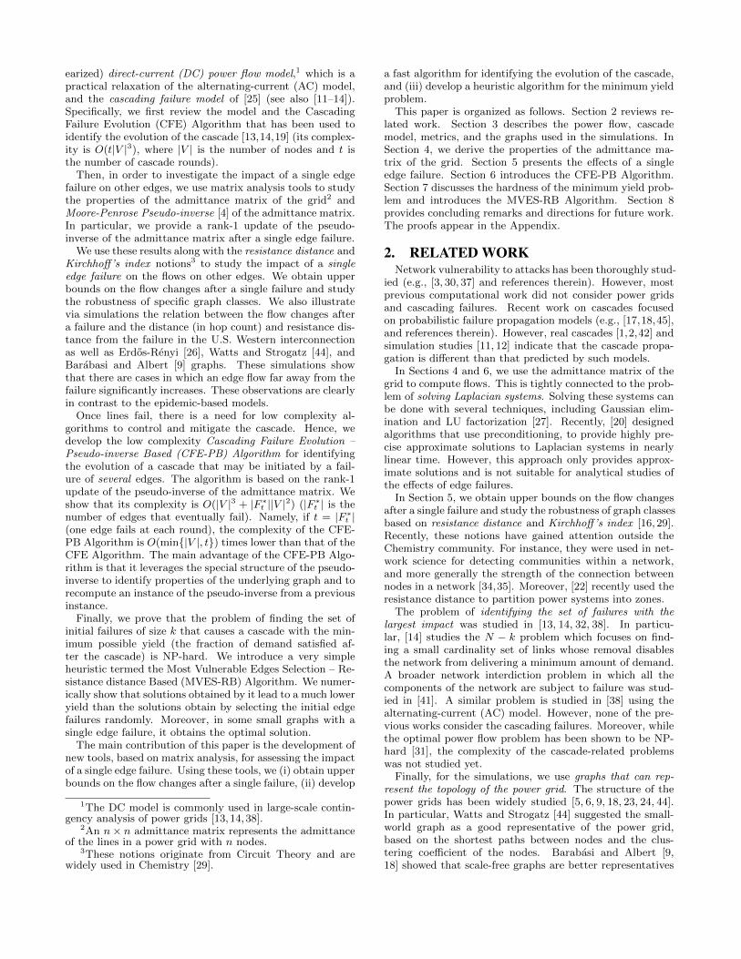
An example of a cascade can be seen in Fig. 2. Initially,the flows are fe = 0.5 for all edges. The initial set of failures(F0) disconnects a demand node from the graph. Hence,intuitively, one may not expect a cascade. However, thisinitial failure not only causes further failures but also causesfailures in all edges except for two. This example can begeneralized to a graph with 2n nodes where with the sameset of initial failures, all the edges fail except for two.
For simplicity, when the initial failure event contains asingle edge, F0 = e′, we denote the flows after the failureby f ′e ≡ fe(e′) and the flow changes by ∆fe = f ′e−fe ∀e ∈E\e′.
3.3 MetricsTo study the effects of a single edge (e′) failure after one
round, we define the ratio between the change of flow on anedge, e, and its original value or the flow value on the failededge, e′:
5Note that [12, 14, 25] maintain moving averages of thefe values to determine which edges fail.
F0
(a) Initial flows and the fail-ure event (F0).
F1
(b) Flows and failures due tooverload (F1).
F2
(c) Flows and failures (F2).
0
0
0
0
0
1/2
1/2
-1
1/2
1/2
(d) Stable state.
Figure 2: An example of a cascading failure initiated by outages of the edges connecting a demand node to the network. Theedge capacities and reactance values are ce = 0.6, xe = 1. Numbers in nodes indicate power supply or demand (pv), numberson edges indicate flows (fe), and arrows indicate flow direction.
Edge flow change ratio: Se,e′ = |∆fe/fe|.Mutual edge flow change ratio: Me,e′ = |∆fe/fe′ |.
Below, we define a metric related to the evaluation of thecascade severity for a given instance G, an initial failureevent F0 ⊆ E, and an integer k ≥ 1. An instance is com-posed of a connected graph G, supply/demand vector P ,capacities and reactance values ce, xe ∀e ∈ E. For brevity,an instance is represented by G.Yield (the ratio between the demand supplied at stabi-lization and the original demand): Y (G,F0), Y (G, k) =minF0⊆E,|F0|≤k Y (G,F0).
3.4 Graphs Used in SimulationsThe simulation results are presented for the graphs de-
scribed below. All graphs have 1,374 nodes to correspondthe subgraph of the Western interconnection. The parame-ters are as indicted below, unless otherwise mentioned.Western interconnection: 1708-edge connected subgraphof the U.S. Western interconnection. The data is from thePlatts Geographic Information System (GIS) [39].Erdos-Renyi graph [26]: A random graph where each edgeappears with probability p = 0.01.Watts and Strogatz graph [44]: A small-world randomgraph where each node connects to k = 4 other nodes andthe probability of rewiring is p = 0.1.Barabasi and Albert graph [9]: A scale-free randomgraph where each new node connects to k = 3 other nodes ateach step following the preferential attachment mechanism.
4. ADMITTANCE MATRIX PROPERTIESIn this section, we use the Moore-Penrose Pseudo-inverse
of the admittance matrix [4] in order to obtain results thatare used throughout the rest of the paper. Specifically theyare used in Section 5 to study the impact of a single edgefailure on the flows on other edges and in Section 6 to intro-duce an efficient algorithm to identify the evolution of thecascade. We prove several properties of the Pseudo-inverseof the admittance matrix A, denoted by A+.6 A+ always ex-ists regardless of the structure of the graph G. Some proofsand results that are used in the proofs appear in the Ap-pendix.
Observation 1 shows that the power flow equations can besolved by using A+.
6A+ = limδ→0 At(AAt+δ2I)−1 [4]. For more information
regarding the definition, see Appendix.
Observation 1. If (3) has a feasible solution, Θ = A+Pis a solution for (3).7
Proof. According to Theorem A.1, Θ = A+P minimizes‖P − AΘ‖. On the other hand, since (3) has a solution,
‖P − AΘ‖ = minΘ ‖P − AΘ‖ = 0. Thus, Θ = A+P is asolution for (3).
Jointly verifying whether an edge is a cut-edge and findingthe connected components of the graph takes O(|E|) (us-ing Depth First Search [21]). The following two Lemmasshow that by using the precomputed pseudo-inverse of theadmittance matrix, these operations can be done in O(1)and O(|V |), respectively. The algorithm in Section ?? usesthe results to check if the pseudo-inverse should be recom-puted. Moreover, Lemma 1 is crucial for the proof of theTheorem 1, below.
Lemma 1 (Bapat [8]). Given G = (V,E) and A+, allthe cut-edges of the graph G can be found in O(|E|) time.Specifically, an edge i, j ∈ E is a cut-edge if, and only if,a−1ij − 2a+
ij + a+ii + a+
jj = 0.
Lemma 2. Given G = (V,E), A+, and the cut-edge i, j,the connected components of G\i, j can be identified inO(|V |).
In the following, we denote by A′ the admittance matrix ofthe graph G′ = (V,E\i, j) and by P ′ the power vector af-ter removing an arbitrary edge e′ = i, j from the graph Gand conducting the corresponding load shedding/generationcurtailing.
Lemma 3 shows that after the removal of a cut-edge, A+
can be used to solve (3) and A′+ is not required.Lemma 3. Given graph G = (V,E), A+, and a cut-edge
i, j, then Θ = A+P ′ is a solution of (3) in G′.The following theorem gives an analytical rank-1 update ofthe pseudo-inverse of the admittance matrix. Using Theo-rem 1 and Corollary 1, in Section 5 we provide upper boundson the mutual edge flow change ratios (Me,e′). We note thata similar result to Theorem 1 was independently proved ina very recent technical report [40].
Theorem 1. Given graph G = (V,E), the admittancematrix A, and A+, if i, j is not a cut-edge, then,
A′+ = (A+ aijXXt)+ = A+ − 1
a−1ij +XtA+X
A+XXtA+
in which X is an n× 1 vector with 1 in ith entry, −1 in jth
entry, and 0 elsewhere.7Recall from Section 3 that (1)-(2) have a unique solu-
tion with respect to power flows but not in respect to phaseangles. Therefore, the solution to (3) may not be unique.
−5 0 5 10 15 20 25 30 35 40Distance (d(i,j))
(a) Western interconnection
−5
0
5
10
15
20
25
30
35
Res
ista
nce
Dis
tan
ce (r(i,j))
1 2 3Distance (d(i,j))
(b) Erdos Renyi graph
0.008
0.010
0.012
0.014
0.016
0.018
0.020
0.022
0 5 10 15 20Distance (d(i,j))
(c) Watts and Strogatz graph
0.0
0.5
1.0
1.5
2.0
2.5
3.0
0 1 2 3 4 5 6 7Distance (d(i,j))
(d) Barabasi and Albert graph
−0.2
0.0
0.2
0.4
0.6
0.8
1.0
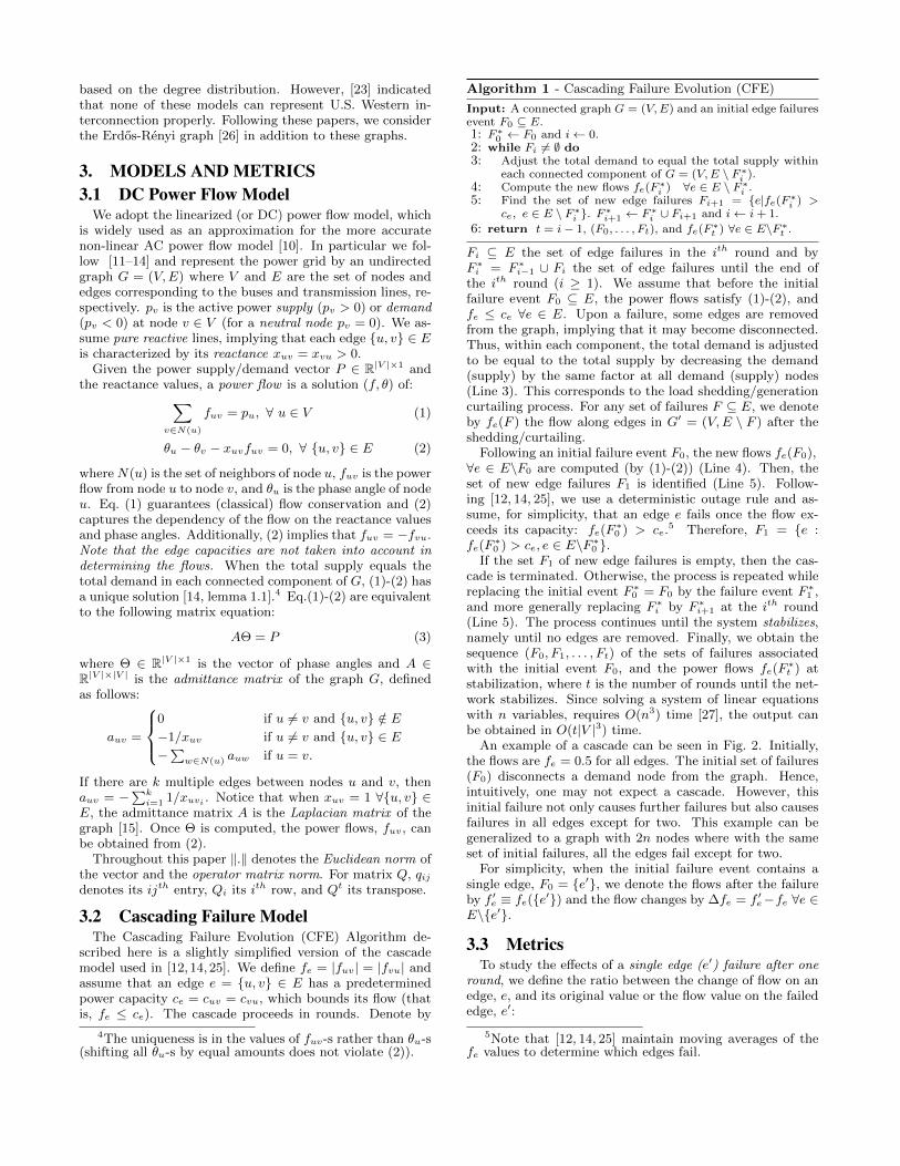
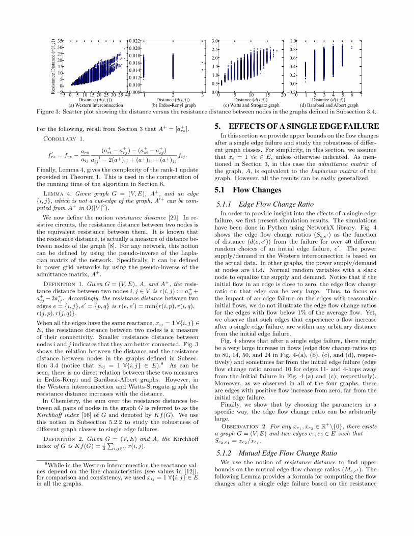
Figure 3: Scatter plot showing the distance versus the resistance distance between nodes in the graphs defined in Subsection 3.4.
For the following, recall from Section 3 that A+ = [a+rs].
Corollary 1.
f ′rs = frs −arsaij
(a+ri − a
+rj)− (a+
si − a+sj)
a−1ij − 2(a+)ij + (a+)ii + (a+)jj
fij .
Finally, Lemma 4, gives the complexity of the rank-1 updateprovided in Theorem 1. This is used in the computation ofthe running time of the algorithm in Section 6.
Lemma 4. Given graph G = (V,E), A+, and an edgei, j, which is not a cut-edge of the graph, A′+ can be com-puted from A+ in O(|V |2).
We now define the notion resistance distance [29]. In re-sistive circuits, the resistance distance between two nodes isthe equivalent resistance between them. It is known thatthe resistance distance, is actually a measure of distance be-tween nodes of the graph [8]. For any network, this notioncan be defined by using the pseudo-inverse of the Lapla-cian matrix of the network. Specifically, it can be definedin power grid networks by using the pseudo-inverse of theadmittance matrix, A+.
Definition 1. Given G = (V,E), A, and A+, the resis-tance distance between two nodes i, j ∈ V is r(i, j) := a+
ii +a+jj − 2a+
ij. Accordingly, the resistance distance between two
edges e = i, j, e′ = p, q is r(e, e′) = minr(i, p), r(i, q),r(j, p), r(j, q).When all the edges have the same reactance, xij = 1 ∀i, j ∈E, the resistance distance between two nodes is a measureof their connectivity. Smaller resistance distance betweennodes i and j indicates that they are better connected. Fig. 3shows the relation between the distance and the resistancedistance between nodes in the graphs defined in Subsec-tion 3.4 (notice that xij = 1 ∀i, j ∈ E).8 As can beseen, there is no direct relation between these two measuresin Erdos-Renyi and Barabasi-Albert graphs. However, inthe Western interconnection and Watts-Strogatz graph theresistance distance increases with the distance.
In Chemistry, the sum over the resistance distances be-tween all pairs of nodes in the graph G is referred to as theKirchhoff index [16] of G and denoted by Kf(G). We usethis notion in Subsection 5.2.2 to study the robustness ofdifferent graph classes to single edge failures.
Definition 2. Given G = (V,E) and A, the Kirchhoffindex of G is Kf(G) = 1
2
∑i,j∈V r(i, j).
8While in the Western interconnection the reactance val-ues depend on the line characteristics (see values in [12]),for comparison and consistency, we used xij = 1 ∀i, j ∈ Ein all the graphs.
5. EFFECTS OF A SINGLE EDGE FAILUREIn this section we provide upper bounds on the flow changes
after a single edge failure and study the robustness of differ-ent graph classes. For simplicity, in this section, we assumethat xe = 1 ∀e ∈ E, unless otherwise indicated. As men-tioned in Section 3, in this case the admittance matrix ofthe graph, A, is equivalent to the Laplacian matrix of thegraph. However, all the results can be easily generalized.
5.1 Flow Changes
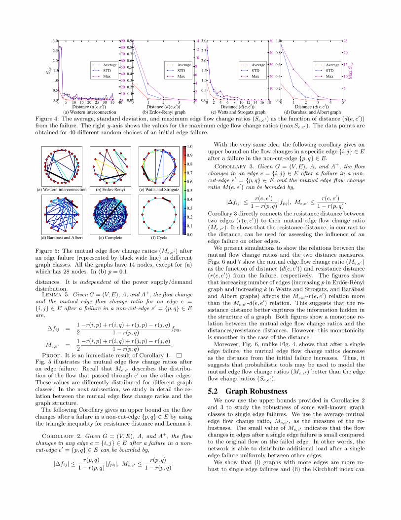
5.1.1 Edge Flow Change RatioIn order to provide insight into the effects of a single edge
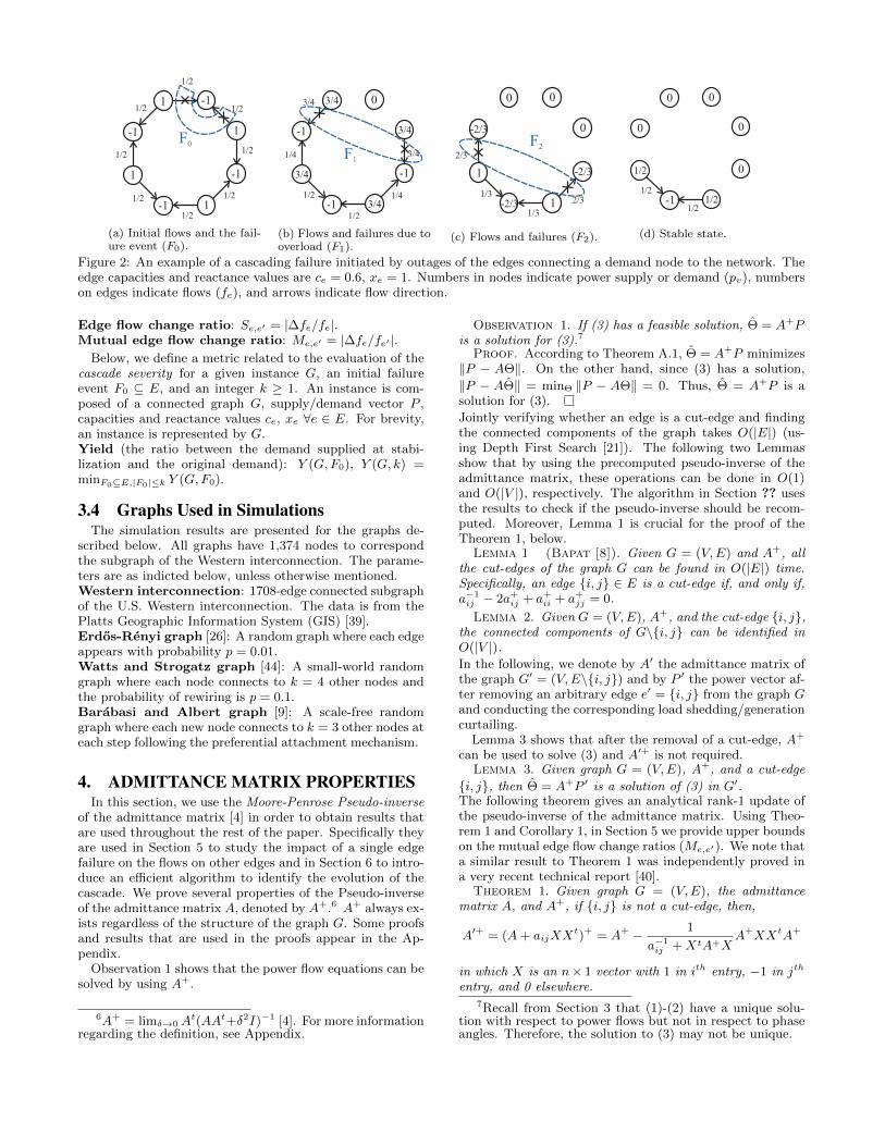
failure, we first present simulation results. The simulationshave been done in Python using NetworkX library. Fig. 4shows the edge flow change ratios (Se,e′) as the functionof distance (d(e, e′)) from the failure for over 40 differentrandom choices of an initial edge failure, e′. The powersupply/demand in the Western interconnection is based onthe actual data. In other graphs, the power supply/demandat nodes are i.i.d. Normal random variables with a slacknode to equalize the supply and demand. Notice that if theinitial flow in an edge is close to zero, the edge flow changeratio on that edge can be very large. Thus, to focus onthe impact of an edge failure on the edges with reasonableinitial flows, we do not illustrate the edge flow change ratiosfor the edges with flow below 1% of the average flow. Yet,we observe that such edges that experience a flow increaseafter a single edge failure, are within any arbitrary distancefrom the initial edge failure.
Fig. 4 shows that after a single edge failure, there mightbe a very large increase in flows (edge flow change ratios upto 80, 14, 50, and 24 in Fig. 4-(a), (b), (c), and (d), respec-tively) and sometimes far from the initial edge failure (edgeflow change ratio around 10 for edges 11- and 4-hops awayfrom the initial failure in Fig. 4-(a) and (c), respectively).Moreover, as we observed in all of the four graphs, thereare edges with positive flow increase from zero, far from theinitial edge failure.
Finally, we show that by choosing the parameters in aspecific way, the edge flow change ratio can be arbitrarilylarge.
Observation 2. For any xe1 , xe2 ∈ R+\0, there existsa graph G = (V,E) and two edges e1, e2 ∈ E such thatSe2,e1 = xe2/xe1 .
5.1.2 Mutual Edge Flow Change RatioWe use the notion of resistance distance to find upper
bounds on the mutual edge flow change ratios (Me,e′). Thefollowing Lemma provides a formula for computing the flowchanges after a single edge failure based on the resistance
0 5 10 15 20 25 30 35 40Distance (d(e,e′))
(a) Western interconnection
0.0
0.5
1.0
1.5
2.0
2.5
3.0
Se,e
′
Average
STD
Max
0
10
20
30
40
50
60
70
80
90
0 1 2 3 4Distance (d(e,e′))
(b) Erdos-Renyi graph
0.0
0.1
0.2
0.3
0.4
0.5
0.6
0.7
0.8
0.9
Average
STD
Max
0
2
4
6
8
10
12
14
0 2 4 6 8 10 12 14 16 18Distance (d(e,e′))
(c) Watts and Strogatz graph
0.0
0.5
1.0
1.5
2.0
2.5
3.0
Average
STD
Max
0
10
20
30
40
50
0 1 2 3 4 5
Distance (d(e,e′)) (d) Barabasi and Albert graph
0.0
0.2
0.4
0.6
0.8
1.0
Average
STD
Max
0
5
10
15
20
25
Max
Se,e
′
Figure 4: The average, standard deviation, and maximum edge flow change ratios (Se,e′) as the function of distance (d(e, e′))from the failure. The right y-axis shows the values for the maximum edge flow change ratios (maxSe,e′). The data points areobtained for 40 different random choices of an initial edge failure.
(a) Western interconnection (b) Erdos-Renyi
(f) Cycle(e) Complete(d) Barabasi and Albert
(c) Watts and Strogatz
0.0
0.1
0.2
0.3
0.4
0.5
0.6
0.7
0.8
0.9
1.0
Figure 5: The mutual edge flow change ratios (Me,e′) afteran edge failure (represented by black wide line) in differentgraph classes. All the graphs have 14 nodes, except for (a)which has 28 nodes. In (b) p = 0.1.
distances. It is independent of the power supply/demanddistribution.
Lemma 5. Given G = (V,E), A, and A+, the flow changeand the mutual edge flow change ratio for an edge e =i, j ∈ E after a failure in a non-cut-edge e′ = p, q ∈ Eare,
∆fij =1
2
−r(i, p) + r(i, q) + r(j, p)− r(j, q)1− r(p, q) fpq,
Me,e′ =1
2
−r(i, p) + r(i, q) + r(j, p)− r(j, q)1− r(p, q) .
Proof. It is an immediate result of Corollary 1.Fig. 5 illustrates the mutual edge flow change ratios afteran edge failure. Recall that Me,e′ describes the distribu-tion of the flow that passed through e′ on the other edges.These values are differently distributed for different graphclasses. In the next subsection, we study in detail the re-lation between the mutual edge flow change ratios and thegraph structure.
The following Corollary gives an upper bound on the flowchanges after a failure in a non-cut-edge p, q ∈ E by usingthe triangle inequality for resistance distance and Lemma 5.
Corollary 2. Given G = (V,E), A, and A+, the flowchanges in any edge e = i, j ∈ E after a failure in a non-cut-edge e′ = p, q ∈ E can be bounded by,
|∆fij | ≤r(p, q)
1− r(p, q) |fpq|, Me,e′ ≤r(p, q)
1− r(p, q) .
With the very same idea, the following corollary gives anupper bound on the flow changes in a specific edge i, j ∈ Eafter a failure in the non-cut-edge p, q ∈ E.
Corollary 3. Given G = (V,E), A, and A+, the flowchanges in an edge e = i, j ∈ E after a failure in a non-cut-edge e′ = p, q ∈ E and the mutual edge flow changeratio M(e, e′) can be bounded by,
|∆fij | ≤r(e, e′)
1− r(p, q) |fpq|, Me,e′ ≤r(e, e′)
1− r(p, q) .
Corollary 3 directly connects the resistance distance betweentwo edges (r(e, e′)) to their mutual edge flow change ratio(Me,e′). It shows that the resistance distance, in contrast tothe distance, can be used for assessing the influence of anedge failure on other edges.
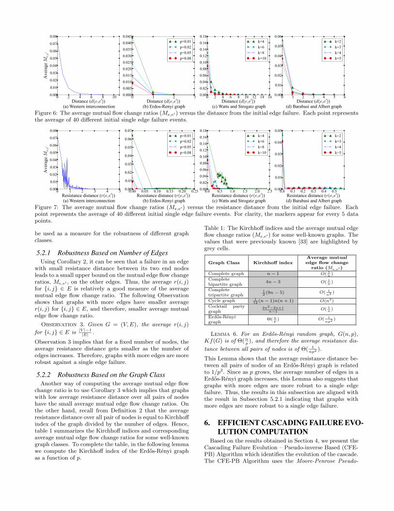
We present simulations to show the relations between themutual flow change ratios and the two distance measures.Figs. 6 and 7 show the mutual edge flow change ratio (Me,e′)as the function of distance (d(e, e′)) and resistance distance(r(e, e′)) from the failure, respectively. The figures showthat increasing number of edges (increasing p in Erdos-Renyigraph and increasing k in Watts and Strogatz, and Barabasiand Albert graphs) affects the Me,e′ -r(e, e
′) relation morethan the Me,e′ -d(e, e′) relation. This suggests that the re-sistance distance better captures the information hidden inthe structure of a graph. Both figures show a monotone re-lation between the mutual edge flow change ratios and thedistances/resistance distances. However, this monotonicityis smoother in the case of the distance.
Moreover, Fig. 6, unlike Fig. 4, shows that after a singleedge failure, the mutual edge flow change ratios decreaseas the distance from the initial failure increases. Thus, itsuggests that probabilistic tools may be used to model themutual edge flow change ratios (Me,e′) better than the edgeflow change ratios (Se,e′).
5.2 Graph RobustnessWe now use the upper bounds provided in Corollaries 2
and 3 to study the robustness of some well-known graphclasses to single edge failures. We use the average mutualedge flow change ratio, Me,e′ , as the measure of the ro-bustness. The small value of Me,e′ indicates that the flowchanges in edges after a single edge failure is small comparedto the original flow on the failed edge. In other words, thenetwork is able to distribute additional load after a singleedge failure uniformly between other edges.
We show that (i) graphs with more edges are more ro-bust to single edge failures and (ii) the Kirchhoff index can
0 2 4 6 8 10Distance (d(e,e′))
(a) Western interconnection
0.00
0.01
0.02
0.03
0.04
0.05
0.06
0.07
0.08
Aver
age M
e,e
′
0 1 2 3Distance (d(e,e′))
(b) Erdos-Renyi graph
0.000
0.005
0.010
0.015
0.020
0.025
0.030
0.035
0.040
0.045
p=0.01
p=0.02
p=0.05
p=0.08
0 2 4 6 8 10 12 14 16Distance (d(e,e′))
(c) Watts and Strogatz graph
0.00
0.02
0.04
0.06
0.08
0.10
0.12
0.14
0.16
0.18
k=4
k=6
k=8
k=10
0 1 2 3 4 5 6Distance (d(e,e′))
(d) Barabasi and Albert graph
0.00
0.01
0.02
0.03
0.04
0.05
0.06
k=2
k=3
k=4
k=5
Figure 6: The average mutual flow change ratios (Me,e′) versus the distance from the initial edge failure. Each point representsthe average of 40 different initial single edge failure events.
0 1 2 3 4 5
Resistance distance (r(e,e′)) (a) Western interconnection
0.00
0.01
0.02
0.03
0.04
0.05
0.06
0.07
0.08
Aver
age M
e,e
′
0.00 0.05 0.10 0.15 0.20 0.25Resistance distance (r(e,e′))
(b) Erdos-Renyi graph
0.00
0.01
0.02
0.03
0.04
0.05
0.06
0.07
p=0.01
p=0.02
p=0.05
p=0.08
0.0 0.5 1.0 1.5 2.0 2.5Resistance distance (r(e,e′)) (c) Watts and Strogatz graph
0.00
0.02
0.04
0.06
0.08
0.10
0.12
0.14
0.16
0.18
k=4
k=6
k=8
k=10
0.0 0.1 0.2 0.3 0.4 0.5Resistance distance (r(e,e′))
(d) Barabasi and Albert graph
0.00
0.01
0.02
0.03
0.04
0.05
k=2
k=3
k=4
k=5
Figure 7: The average mutual flow change ratios (Me,e′) versus the resistance distance from the initial edge failure. Eachpoint represents the average of 40 different initial single edge failure events. For clarity, the markers appear for every 5 datapoints.
be used as a measure for the robustness of different graphclasses.
5.2.1 Robustness Based on Number of EdgesUsing Corollary 2, it can be seen that a failure in an edge
with small resistance distance between its two end nodesleads to a small upper bound on the mutual edge flow changeratios, Me,e′ , on the other edges. Thus, the average r(i, j)for i, j ∈ E is relatively a good measure of the averagemutual edge flow change ratio. The following Observationshows that graphs with more edges have smaller averager(i, j) for i, j ∈ E, and therefore, smaller average mutualedge flow change ratio.
Observation 3. Given G = (V,E), the average r(i, j)
for i, j ∈ E is |V |−1|E| .
Observation 3 implies that for a fixed number of nodes, theaverage resistance distance gets smaller as the number ofedges increases. Therefore, graphs with more edges are morerobust against a single edge failure.
5.2.2 Robustness Based on the Graph ClassAnother way of computing the average mutual edge flow
change ratio is to use Corollary 3 which implies that graphswith low average resistance distance over all pairs of nodeshave the small average mutual edge flow change ratios. Onthe other hand, recall from Definition 2 that the averageresistance distance over all pair of nodes is equal to Kirchhoffindex of the graph divided by the number of edges. Hence,table 1 summarizes the Kirchhoff indices and correspondingaverage mutual edge flow change ratios for some well-knowngraph classes. To complete the table, in the following lemmawe compute the Kirchhoff index of the Erdos-Renyi graphas a function of p.
Table 1: The Kirchhoff indices and the average mutual edgeflow change ratios (Me,e′) for some well-known graphs. Thevalues that were previously known [33] are highlighted bygrey cells.
Graph Class Kirchhoff indexAverage mutualedge flow change
ratio (Me,e′)
Complete graph n − 1 O( 1n )
Completebipartite graph
4n − 3 O( 1n )
Completetripartite graph
12 (9n − 5) O( 1
n2 )
Cycle graph 112 (n − 1)n(n + 1) O(n2)
Cocktail partygraph
2n2−2n+1n−1
O( 1n )
Erdos-Renyigraph
Θ( np ) O( 1
np2)
Lemma 6. For an Erdos-Renyi random graph, G(n, p),Kf(G) is of Θ(n
p), and therefore the average resistance dis-
tance between all pairs of nodes is of Θ( 1np2
).
This Lemma shows that the average resistance distance be-tween all pairs of nodes of an Erdos-Renyi graph is relatedto 1/p2. Since as p grows, the average number of edges in aErdos-Renyi graph increases, this Lemma also suggests thatgraphs with more edges are more robust to a single edgefailure. Thus, the results in this subsection are aligned withthe result in Subsection 5.2.1 indicating that graphs withmore edges are more robust to a single edge failure.
6. EFFICIENT CASCADING FAILURE EVO-LUTION COMPUTATION
Based on the results obtained in Section 4, we present theCascading Failure Evolution – Pseudo-inverse Based (CFE-PB) Algorithm which identifies the evolution of the cascade.The CFE-PB Algorithm uses the Moore-Penrose Pseudo-
Algorithm 2 - Cascading Failure Evolution – Pseudo-inverse Based (CFE-PB)
Input: A connected graph G = (V,E) and an initial edge failuresevent F0 ⊆ E.1: Compute A+, F ∗0 ← F0 and i← 0.2: while Fi 6= ∅ do3: for each r, s ∈ Fi do4: if r, s is a cut-edge (see Lemma 1) then5: Find the connected components after removing r, s.
(see Lemma 2)6: Adjust the total demand to equal the total supply
within each connected component.7: else update A+ after removing r, s. (see Lemma 4)
8: Compute the phase angles Θ = A+P and compute newflows fe(F ∗i ) from the phase angles.
9: Find the set of new edge failures Fi+1 = e|fe > ce, e ∈E \ F ∗i . F ∗i+1 ← F ∗i ∪ Fi+1 and i← i + 1.
10: return t = i− 1, (F0, . . . , Ft), and fe(F ∗t ) ∀e ∈ E\F ∗t .
inverse of the admittance matrix for solving (3). Comput-ing the pseudo-inverse of the admittance matrix requiresO(|V |3) time. However, the algorithm obtains the pseudo-inverse of the admittance matrix in round i from the oneobtained in round (i− 1), in O(|Fi||V |2) time. Moreover, insome cases, the algorithm can reuse the pseudo-inverse fromthe previous round. Since once lines fail, there is a need forlow complexity algorithms to control and mitigate the cas-cade, the CFE-PB Algorithm may provide insight into thedesign of efficient cascade control algorithms.
We now describe the CFE-PB Algorithm. It initiallycomputes the pseudo-inverse of the admittance matrix (inO(|V |3) time) and this is the only time in which it computesA+ without using a previous version of A+. Next, startingfrom F0, at each round of the cascade, for each e ∈ Fi, itchecks whether e is a cut-edge (Line 4). This is done in O(1)(Lemma 1). If yes, based on Lemma 3, in Lines 5 and 6, thetotal demand is adjusted to equal the total supply withineach connected component (in O(V ) time). Else, in Line 7,A+ after the removal of e is computed in O(|V |2) time (seeLemma 4). After repeating this process for each e ∈ Fi, thephase angles and the flows are computed in O(|V |2) time(Line 8). The rest of the process is similar to the CFE Al-gorithm.
The following theorem provides the complexity of the al-gorithm (the proof is based on the Lemmas 1–4). We showthat the algorithm runs in O(|V |3 + |F ∗t ||V |2) time (com-pared to the CFE Algorithm which runs inO(t|V |3)). Namely,if t = |F ∗t | (one edge fails at each round), the CFE-PB Algo-rithm outperforms the CFE Algorithms by O(min|V |, t).
Theorem 2. CFE-PB Algorithm runs in O(|V |3+|F ∗t ||V |2)time.We notice that a similar approach (the step by step rank-1update) can also be applied to other methods for solving lin-ear equations (e.g., LU factorization [27]). However, as weshowed in Section 5, using the pseudo-inverse allows devel-oping tools for analyzing the effect of a single edge failure.Moreover, it supports the development of an algorithm forfinding the most vulnerable edges.
7. HARDNESS AND HEURISTICIn this section, we prove that the decision problem asso-
ciated with the minimum yield is NP-complete. Using theresults from Section 5, we introduce a heuristic algorithmfor the problem of finding the set of initial failures of size
Algorithm 3 - Most Vulnerable Edges Selection – Resis-tance distance Based (MVES-RB)
Input: A connected graph G = (V,E) and an integer k ≥ 1.1: Compute A+.
2: Compute the phase angles Θ = A+P and compute flows fefrom the phase angles.
3: Compute the resistance distance r(i, j) = r(e) ∀e = i, j ∈E.
4: Sort edges e1, e2, . . . , e|E| such that p ≤ q iff fepr(ep) ≥feq r(eq).
5: return e1, e2, . . . , ek.
k that causes a cascade resulting with the minimum possi-ble yield (minimum yield problem). We numerically showthat solutions obtained by the heuristic algorithm lead toa much lower yield than the solutions obtain by selectingthe initial edge failures randomly. Moreover, in some smallgraphs with a single edge failure, this algorithm obtains theoptimal solution.
First, we show that deciding if there exists a failure event(of size at most a given value) such that the yield after sta-bilization is less than a given threshold, is NP-complete.
Lemma 7. Given a graph G, a real number y, 0 ≤ y ≤ 1,and an integer k ≥ 1, the problem of deciding if Y (G, k) ≤ yis NP-complete.
We now present a heuristic algorithm for solving this prob-lem. We refer to it as the Most Vulnerable Edge Selection– Resistance distance Based (MVES-RB) Algorithm. FromCorollary 2, it seems that edges with large r(i, j) × |fij |have greater impact on the flow changes on the other edges.Based on this result, the MVES-RB Algorithm selects the kedges with highest r(i, j) × |fij | values as the initial set offailures.
The MVES-RB Algorithm is in the same category as thealgorithms that identify the set of failures with the largestimpact (i.e., algorithms that solve the N−k problem [14,32,38]). However, none of the previous works focusing on theN−k problem, considers cascading failures. The MVES-RBAlgorithm is simpler than most of the algorithms proposedin the past. However, it is not possible to compare its per-formance to that of algorithms in [14, 32, 38, 41] since theyuse different formulations of the power flow problem.
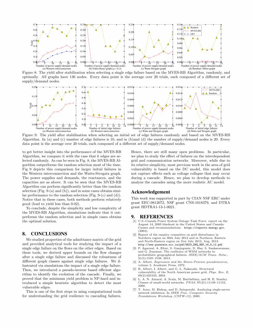
We first compare via simulation the MVES-RB Algorithmto the optimal solution in small graphs and for a single initialedge failure. Fig. 8 shows the yield after stabilization whenselecting a single edge failure based on the MVES-RB Al-gorithm, randomly, and optimally. All the graphs have 136nodes. For all the edges the reactance, xe = 1,9 and the ca-pacity ce = 1.1fe,
10 where fe is the initial flow on the edge.At each point, equal number of power supply and demandnodes are randomly selected and assigned values of 1 and -1.As can be seen, the MVES-RB Algorithm obtains the op-timal solution in Erdos-Renyi and Barabasi-Albert graphs.However, it does not achieve the optimal solution in theWestern interconnection and Watts-Strogatz graph.
Finding the optimal solution for the minimum yield prob-lem in the general case is impossible in practice. Therefore,
9While in the Western interconnection the reactance val-ues depend on the line characteristics (see values in [12]),for comparison and consistency, we used xij = 1 ∀i, j ∈ Ein all the graphs.
10Following [12], we assume that the capacities are Ktimes the initial flows on the edges. K is often referredto as the Factor of Safety (FoS) of the grid. Here, K = 1.1as in [12].
0 5 10 15 20 25Number of power supply/demand nodes
(a) Western interconnection
0.0
0.1
0.2
0.3
0.4
0.5
0.6
0.7
Yie
ld
0 5 10 15 20 25Number of power supply/demand nodes
(b) Erdos-Renyi graph (p=0.2)
0.00
0.05
0.10
0.15
0.20
0.25
0.30
0.35
0 5 10 15 20 25Number of power supply/demand nodes
(c) Watts-Strogatz graph
0.00
0.05
0.10
0.15
0.20
0.25
0 5 10 15 20 25Number of power supply/demand nodes
(d) Barabasi-Albert graph
0.00
0.02
0.04
0.06
0.08
0.10
0.12
0.14
0.16Random
MVES-RB
OPT
Figure 8: The yield after stabilization when selecting a single edge failure based on the MVES-RB Algorithm, randomly, andoptimally. All graphs have 136 nodes. Every data point is the average over 20 trials, each composed of a different set ofsupply/demand nodes.
0 5 10 15 20 25 30Number of power supply/demand nodes
(a) Western interconnection
0.00
0.05
0.10
0.15
0.20
Yie
ld
0 2 4 6 8 10 12 14Number of initial edge failures (b) Western interconnection
0.0
0.1
0.2
0.3
0.4
0.5
0.6
0.7
0 5 10 15 20 25 30Number of power supply/demand nodes
(c) Watts and Strogatz graph
0.000
0.002
0.004
0.006
0.008
0.010
0.012
0 2 4 6 8 10 12 14Number of initial edge failures (d) Watts and Strogatz graph
0.004
0.006
0.008
0.010
0.012
0.014
0.016MVES-RB
Random
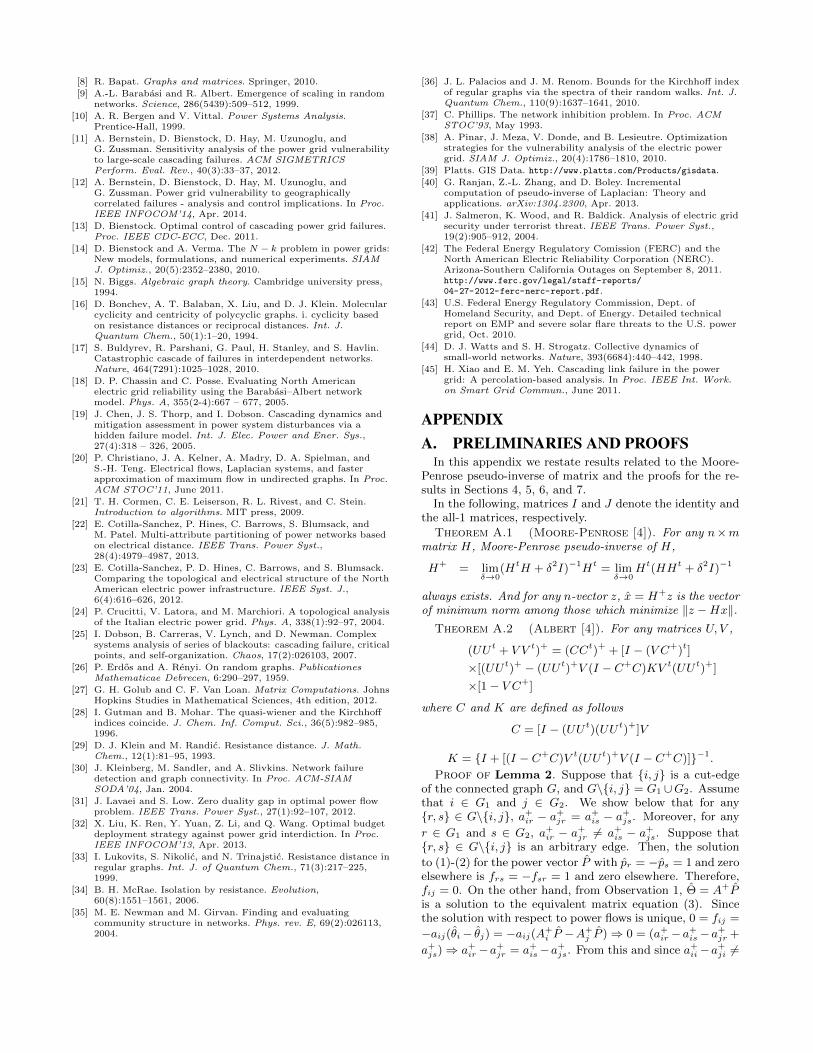
Figure 9: The yield after stabilization when selecting an initial set of edge failures randomly and based on the MVES-RBAlgorithm. In (a) and (c) number of edge failures is 10, and in (b)and (d) the number of supply/demand nodes is 20. Everydata point is the average over 20 trials, each composed of a different set of supply/demand nodes.
to get better insight into the performance of the MVES-RBAlgorithm, we compare it with the case that k edges are se-lected randomly. As can be seen in Fig. 8, the MVES-RB Al-gorithm outperforms the random selection most of the time.Fig 9 depicts this comparison for larger initial failures inthe Western interconnection and the Watts-Strogatz graph.The power supplies and demands, the reactances, and thecapacities are as above. It can be seen that the MVES-RBAlgorithm can perform significantly better than the randomselection (Fig. 9-(a) and (b)), and in some cases obtains simi-lar performance to the random selection (Fig. 9-(c) and (d)).Notice that in these cases, both methods perform relativelygood (lead to yield less than 0.02).
To conclude, despite the simplicity and low complexity ofthe MVES-RB Algorithm, simulations indicate that it out-performs the random selection and in simple cases obtainsthe optimal solution.
8. CONCLUSIONSWe studied properties of the admittance matrix of the grid
and provided analytical tools for studying the impact of asingle edge failure on the flows on the other edges. Based onthese tools, we derived upper bounds on the flow changesafter a single edge failure and discussed the robustness ofdifferent graph classes against single edge failures. We il-lustrated via simulations the impact of a single edge failure.Then, we introduced a pseudo-inverse based efficient algo-rithm to identify the evolution of the cascade. Finally, weproved that the minimum yield problem is NP-hard and in-troduced a simple heuristic algorithm to detect the mostvulnerable edges.
This is one of the first steps in using computational toolsfor understanding the grid resilience to cascading failures.
Hence, there are still many open problems. In particular,we plan to study the effect of failures on the interdependentgrid and communication networks. Moreover, while due toits relative simplicity, most previous work in the area of gridvulnerability is based on the DC model, this model doesnot capture effects such as voltage collapse that may occurduring a cascade. Hence, we plan to develop methods toanalyze the cascades using the more realistic AC model.
AcknowledgementThis work was supported in part by CIAN NSF ERC undergrant EEC-0812072, NSF grant CNS-1018379, and DTRAgrant HDTRA1-13-1-0021.
9. REFERENCES[1] U.S.-Canada Power System Outage Task Force. report on the
August 14, 2003 blackout in the United States and Canada:Causes and recommendations. https://reports.energy.gov,(2004).
[2] Report of the enquiry committee on grid disturbance inNorthern region on 30th July 2012 and in Northern, Easternand North-Eastern region on 31st July 2012, Aug. 2012.http://www.powermin.nic.in/pdf/GRID_ENQ_REP_16_8_12.pdf.
[3] P. Agarwal, A. Efrat, S. Ganjugunte, D. Hay, S. Sankararaman,and G. Zussman. The resilience of WDM networks toprobabilistic geographical failures. IEEE/ACM Trans. Netw.,21(5):1525–1538, 2013.
[4] A. Albert. Regression and the Moore-Penrose pseudoinverse,volume 3. Academic Press, 1972.
[5] R. Albert, I. Albert, and G. L. Nakarado. Structuralvulnerability of the North American power grid. Phys. Rev. E,69(2):025103, 2004.
[6] L. A. N. Amaral, A. Scala, M. Barthelemy, and H. E. Stanley.Classes of small-world networks. PNAS, 97(21):11149–11152,2000.
[7] T. Aura, M. Bishop, and D. Sniegowski. Analyzing single-servernetwork inhibition. In IEEE Proc. Computer SecurityFoundations Workshop (CSFW-13), 2000.
[8] R. Bapat. Graphs and matrices. Springer, 2010.
[9] A.-L. Barabasi and R. Albert. Emergence of scaling in randomnetworks. Science, 286(5439):509–512, 1999.
[10] A. R. Bergen and V. Vittal. Power Systems Analysis.Prentice-Hall, 1999.
[11] A. Bernstein, D. Bienstock, D. Hay, M. Uzunoglu, andG. Zussman. Sensitivity analysis of the power grid vulnerabilityto large-scale cascading failures. ACM SIGMETRICSPerform. Eval. Rev., 40(3):33–37, 2012.
[12] A. Bernstein, D. Bienstock, D. Hay, M. Uzunoglu, andG. Zussman. Power grid vulnerability to geographicallycorrelated failures - analysis and control implications. In Proc.IEEE INFOCOM’14, Apr. 2014.
[13] D. Bienstock. Optimal control of cascading power grid failures.Proc. IEEE CDC-ECC, Dec. 2011.
[14] D. Bienstock and A. Verma. The N − k problem in power grids:New models, formulations, and numerical experiments. SIAMJ. Optimiz., 20(5):2352–2380, 2010.
[15] N. Biggs. Algebraic graph theory. Cambridge university press,1994.
[16] D. Bonchev, A. T. Balaban, X. Liu, and D. J. Klein. Molecularcyclicity and centricity of polycyclic graphs. i. cyclicity basedon resistance distances or reciprocal distances. Int. J.Quantum Chem., 50(1):1–20, 1994.
[17] S. Buldyrev, R. Parshani, G. Paul, H. Stanley, and S. Havlin.Catastrophic cascade of failures in interdependent networks.Nature, 464(7291):1025–1028, 2010.
[18] D. P. Chassin and C. Posse. Evaluating North Americanelectric grid reliability using the Barabasi–Albert networkmodel. Phys. A, 355(2-4):667 – 677, 2005.
[19] J. Chen, J. S. Thorp, and I. Dobson. Cascading dynamics andmitigation assessment in power system disturbances via ahidden failure model. Int. J. Elec. Power and Ener. Sys.,27(4):318 – 326, 2005.
[20] P. Christiano, J. A. Kelner, A. Madry, D. A. Spielman, andS.-H. Teng. Electrical flows, Laplacian systems, and fasterapproximation of maximum flow in undirected graphs. In Proc.ACM STOC’11, June 2011.
[21] T. H. Cormen, C. E. Leiserson, R. L. Rivest, and C. Stein.Introduction to algorithms. MIT press, 2009.
[22] E. Cotilla-Sanchez, P. Hines, C. Barrows, S. Blumsack, andM. Patel. Multi-attribute partitioning of power networks basedon electrical distance. IEEE Trans. Power Syst.,28(4):4979–4987, 2013.
[23] E. Cotilla-Sanchez, P. D. Hines, C. Barrows, and S. Blumsack.Comparing the topological and electrical structure of the NorthAmerican electric power infrastructure. IEEE Syst. J.,6(4):616–626, 2012.
[24] P. Crucitti, V. Latora, and M. Marchiori. A topological analysisof the Italian electric power grid. Phys. A, 338(1):92–97, 2004.
[25] I. Dobson, B. Carreras, V. Lynch, and D. Newman. Complexsystems analysis of series of blackouts: cascading failure, criticalpoints, and self-organization. Chaos, 17(2):026103, 2007.
[26] P. Erdos and A. Renyi. On random graphs. PublicationesMathematicae Debrecen, 6:290–297, 1959.
[27] G. H. Golub and C. F. Van Loan. Matrix Computations. JohnsHopkins Studies in Mathematical Sciences, 4th edition, 2012.
[28] I. Gutman and B. Mohar. The quasi-wiener and the Kirchhoffindices coincide. J. Chem. Inf. Comput. Sci., 36(5):982–985,1996.
[29] D. J. Klein and M. Randic. Resistance distance. J. Math.Chem., 12(1):81–95, 1993.
[30] J. Kleinberg, M. Sandler, and A. Slivkins. Network failuredetection and graph connectivity. In Proc. ACM-SIAMSODA’04, Jan. 2004.
[31] J. Lavaei and S. Low. Zero duality gap in optimal power flowproblem. IEEE Trans. Power Syst., 27(1):92–107, 2012.
[32] X. Liu, K. Ren, Y. Yuan, Z. Li, and Q. Wang. Optimal budgetdeployment strategy against power grid interdiction. In Proc.IEEE INFOCOM’13, Apr. 2013.
[33] I. Lukovits, S. Nikolic, and N. Trinajstic. Resistance distance inregular graphs. Int. J. of Quantum Chem., 71(3):217–225,1999.
[34] B. H. McRae. Isolation by resistance. Evolution,60(8):1551–1561, 2006.
[35] M. E. Newman and M. Girvan. Finding and evaluatingcommunity structure in networks. Phys. rev. E, 69(2):026113,2004.
[36] J. L. Palacios and J. M. Renom. Bounds for the Kirchhoff indexof regular graphs via the spectra of their random walks. Int. J.Quantum Chem., 110(9):1637–1641, 2010.
[37] C. Phillips. The network inhibition problem. In Proc. ACMSTOC’93, May 1993.
[38] A. Pinar, J. Meza, V. Donde, and B. Lesieutre. Optimizationstrategies for the vulnerability analysis of the electric powergrid. SIAM J. Optimiz., 20(4):1786–1810, 2010.
[39] Platts. GIS Data. http://www.platts.com/Products/gisdata.
[40] G. Ranjan, Z.-L. Zhang, and D. Boley. Incrementalcomputation of pseudo-inverse of Laplacian: Theory andapplications. arXiv:1304.2300, Apr. 2013.
[41] J. Salmeron, K. Wood, and R. Baldick. Analysis of electric gridsecurity under terrorist threat. IEEE Trans. Power Syst.,19(2):905–912, 2004.
[42] The Federal Energy Regulatory Comission (FERC) and theNorth American Electric Reliability Corporation (NERC).Arizona-Southern California Outages on September 8, 2011.http://www.ferc.gov/legal/staff-reports/04-27-2012-ferc-nerc-report.pdf.
[43] U.S. Federal Energy Regulatory Commission, Dept. ofHomeland Security, and Dept. of Energy. Detailed technicalreport on EMP and severe solar flare threats to the U.S. powergrid, Oct. 2010.
[44] D. J. Watts and S. H. Strogatz. Collective dynamics ofsmall-world networks. Nature, 393(6684):440–442, 1998.
[45] H. Xiao and E. M. Yeh. Cascading link failure in the powergrid: A percolation-based analysis. In Proc. IEEE Int. Work.on Smart Grid Commun., June 2011.
APPENDIXA. PRELIMINARIES AND PROOFS
In this appendix we restate results related to the Moore-Penrose pseudo-inverse of matrix and the proofs for the re-sults in Sections 4, 5, 6, and 7.
In the following, matrices I and J denote the identity andthe all-1 matrices, respectively.
Theorem A.1 (Moore-Penrose [4]). For any n×mmatrix H, Moore-Penrose pseudo-inverse of H,
H+ = limδ→0
(HtH + δ2I)−1Ht = limδ→0
Ht(HHt + δ2I)−1
always exists. And for any n-vector z, x = H+z is the vectorof minimum norm among those which minimize ‖z −Hx‖.
Theorem A.2 (Albert [4]). For any matrices U, V ,
(UU t + V V t)+ = (CCt)+ + [I − (V C+)t]
×[(UU t)+ − (UU t)+V (I − C+C)KV t(UU t)+]
×[1− V C+]
where C and K are defined as follows
C = [I − (UU t)(UU t)+]V
K = I + [(I − C+C)V t(UU t)+V (I − C+C)]−1.
Proof of Lemma 2. Suppose that i, j is a cut-edgeof the connected graph G, and G\i, j = G1 ∪G2. Assumethat i ∈ G1 and j ∈ G2. We show below that for anyr, s ∈ G\i, j, a+
ir − a+jr = a+
is − a+js. Moreover, for any
r ∈ G1 and s ∈ G2, a+ir − a
+jr 6= a+
is − a+js. Suppose that
r, s ∈ G\i, j is an arbitrary edge. Then, the solution
to (1)-(2) for the power vector P with pr = −ps = 1 and zeroelsewhere is frs = −fsr = 1 and zero elsewhere. Therefore,fij = 0. On the other hand, from Observation 1, Θ = A+Pis a solution to the equivalent matrix equation (3). Sincethe solution with respect to power flows is unique, 0 = fij =
−aij(θi− θj) = −aij(A+i P −A
+j P )⇒ 0 = (a+
ir−a+is−a
+jr +
a+js)⇒ a+
ir−a+jr = a+
is−a+js. From this and since a+
ii−a+ji 6=
a+ij − a+
jj (Lemma 1), for any r ∈ G1 and s ∈ G2, a+ir −
a+jr 6= a+
is − a+js. Thus, by using the precomputed pseudo-
inverse of the admittance matrix, computing A+i −A
+j , and
dividing the entries into two groups with equal values, theconnected components of G\i, j can be identified. Thisprocess requires O(|V |) time.
Proof of Lemma 3. First, from Observation 1, Θ =A+P ′ is a solution to (3) for the power vector P ′ in thegraph G. Since the solution to (1)-(2) with respect to power
flows is unique, if fij = 0, then Θ = A+P ′ is also a solutionto (3) for the power vector P ′ in the graph G′. Therefore, we
only need to prove that θi = θj from Θ = A+P ′. To prove
this, we prove that θi − θj = (A+i − A
+j )P ′ = 0. However,
from the proof of Lemma 2, since i, j is a cut-edge, theentries of A+
i − A+j have equal values at the entries in the
same connected component. On the other hand, since P ′ isthe power vector after load shedding/generation curtailing,then the sum of the supplies and demands at each connectedcomponent is zero. Thus, (A+
i −A+j )P ′ = 0.
Proof of Theorem 111. First we show that if G is con-nected, then AA+ = I− 1
nJ . A is a real and symmetric ma-
trix, therefore there exist an orthogonal and unitary matrixU such that A = U tDU , in which D = diag(λ1, λ2, . . . , λn)is the diagonal matrix of eigenvalues of A and Ui is thenormalized eigenvector related to eigenvalue λi. It is well-known that when G is connected and unweighted, then themultiplicity of eigenvalue 0 of the Laplacian matrix is 1 [15].Exactly the same result with the same approach can be ob-tained for weighted graph, therefore we can assume thatλ1 = 0 and all other eigenvalues are nonzero. In this caseU1 = [ 1√
n, 1√
n, . . . , 1√
n]. On the other hand, A+ = U tD+U ,
therefore
AA+ = U tDUU tD+U = U tDD+U
= U tdiag(λ1λ+1 , λ2λ
+2 , . . . , λnλ
+n )U
= U t(I − diag(1, 0, . . . , 0))U
= I − U t[U t1|0| . . . |0]t = I − 1
nJ
in which [U t1|0| . . . |0]t is an n×n matrix with U1 in the firstrow and 0 elsewhere.
Similarly we show that if G has k connected componentswith m1,m2, . . . ,mk nodes, then AA+ = I − Jk in which
Jk = diag(1
m1Jm1×m1 ,
1
m2Jm2×m2 , . . . ,
1
mkJmk×mk )
is a block matrix with matrices on the diagonal entries (withproper node indexing). Suppose G has k ≤ n connectedcomponents. Again it is well-known that when G is un-weighted, multiplicity of eigenvalue 0 of the Laplacian ma-trix is equal to the number of connected components ofgraph G [15]. With exactly the same reasoning it can beshown that it is also the case for weighted graph. There-fore, in this case λ1 = λ2 = · · · = λk = 0. Supposemi is the size of the ith connected component. With aproper indexing of nodes, it is easy to verify that Ui =[0, . . . , 0, 1√
mi, . . . , 1√
mi, 0, . . . , 0], in which uij = 1√
mifor
11The proof provided could be simplified, if the form ofthe A′+ was known in advance. However, the proof showsthe derivation of A′+.
∑i−1k=1 mk < j ≤
∑ik=1 mk, and zero elsewhere. Now similar
to previous part,
AA+ = I − U t[U t1|U t2| . . . |U tk|0| . . . |0]t = I − Jk.
Now we can prove the theorem. A is a real and symmetricmatrix, therefore there exist an n × n matrix B such thatBBt = A. Now using Theorem A.2,
(A+ aijXXt)+ = (CCt)+ + [I − (
√aijXC
+)t]
×[A+ − aijA+X(I − C+C)KXtA+]
×[1−√aijXC+].12
Therefore, all we need to compute is matrices C and K.Using previous part,
C = [I −AA+]X = [I − I + Jk]X = JkX.
Since i, j ∈ E, nodes i and j should be in the same con-nected component of G. Therefore, from the structure ofJk, JkX = 0 and so C = 0. Using this,
K = I + aij [(I − C+C)XtA+X(I − C+C)]−1
= I + aij [IXtA+XI]−1 = 1 + aijX
tA+X−1.
Notice that X is an n × 1 vector, therefore XtA+X is anscaler and I in the second equation is 1× 1. This is why itis written 1 instead of I in the last equation. Since i, j isnot a cut edge, from Lemma 1 we have, 1 + aijX
tA+X =aij [a
−1ij −2(a+)ij + (a+)ii+ (a+)jj ] 6= 0, therefore K is well-
defined. Replacing K and C,
(A+ aijXXt)+
= A+ − aijA+X1 + aijXtA+X−1XtA+
= A+ − 1
a−1ij +XtA+X
A+XXtA+
which is what we wanted to prove.
Proof of Corollary 1. It is easy to see from Theorem 1,
A′+r = A+r −
(a+ri − a
+rj)
a−1ij − 2(a+)ij + (a+)ii + (a+)jj
(A+i −A
+j ).
Using this in f ′rs = −ars(A′+r −A′+s )P completes the proof.
Proof of Lemma 4. Based on Corollary 1, after the re-moval of a non-cut edge i, j, each entry of the pseudo in-verse of the admittance matrix can be updated in O(1) time.Thus, computing A′+ from A+ takes O(|V |2) time.
Proof of Observation 2. We construct the graph G =(V,E) as follows, V = s, t, Ps = −Pt = 1, and thereare two parallel edges e1 and e2 between s and t. Set thecapacities ce1 = ce2 = 1. Assume the reactances xe1 , xe2 aresuch that 0 < xe1 < xe2 .
By Eq. (1)-(2), we get fe1 =xe2
xe2+xe1and fe2 =
xe1xe1+xe2
.
If F0 = e1, then fe2(F0) = 1 and Se2,e1 =xe2xe1
.
Proof of Corollary 2. Using triangle inequality for re-sistance distance, we can write,
−r(i, p) + r(i, q) ≤ r(p, q)r(j, p)− r(j, q) ≤ r(p, q).
Apply these to Lemma 5 completes the proof.
12√aij might be an imaginary number.
Proof of Corollary 3. Notice that r(i, j, p, q) =minr(i, q), r(i, p), r(j, q), r(j, p). The proof is exactly thesame as the proof of Corollary 2.
Proof of Observation 3. From [8, Lemma 9.9], we have∑i,j∈E r(i, j) = |V | − 1 [8].
Proof of Lemma 6. It is known that the Kirchhoff in-dex of the graph G can be written in terms of the eigen-values of the Laplacian matrix of the graph as Kf(G) =n∑n−1i=1
1λi
[28]. On the other hand,
n2 ≤ (
n−1∑i=1
1
λi)(
n−1∑i=1
λi) = (
n−1∑i=1
1
λi)tr(A).
However, when n is relatively big, then each node has thedegree equal to Θ(np), therefore tr(A) = Θ(n2p). Combin-ing this with the equations above, we can easily see thatKf(G) = Ω(n/p). Thus, the average resistance distance isof Kf(G)/|E| = Ω( 1
np2).
As for the upper bound, it is shown in [36] that for a
d-regular graph H with n nodes, Kf(H) ≤ 3n2
d. Using
this bound for Erdos-Renyi graph, we can write Kf(G) =O(n/p). Thus, the average resistance distance is ofO( 1
np2).
Proof of Theorem 2. Finding the pseudo inverse ofthe matrix requires O(|V |3) time. Therefore, Line 1 takesO(|V |3) time. Lines 5 and 6 in the algorithm take O(|V |)time and Line 7 takes O(|V |2), therefore the whole for looptakes at most O(|Fi||V |2) time at each step. Using A+ com-puted in the for loop, Lines 8 and 9 takeO(|V |2) time. Thus,the total running time of the algorithm is at most O(|V |3)+O((|F0|+ |F1|+ · · ·+ |Ft|)|V |2) = O(|V |3)+O(|F ∗t ||V |2).
Proof of Lemma 7. Consider following problem:
Problem 1. Suppose G = (V,E) is an instance of theclassical flow problem, with a single source node s and setof sink nodes T . Assume demands are equal to 1 and lineshave unbounded capacity (O(|V |)). Does a subset of edgesA ⊆ E with |A| ≤ k exist such that |Tfail| ≥ m? (Tfailis set of sink nodes which get disconnected from the sourcenode s after removing set of edges A.)
It is proved in [7, Theorem 7], that problem 1 is NP-complete.We want to use this result to proof Lemma 7. For this rea-son we provide a polynomial time reduction from problemabove to minimum yield problem.
Problem 2. Suppose G = (V,E) is an instance of thepower flow problem, with set of supply node S = s and setof demand nodes T . Assume Pt = −1 for all t ∈ T , andPs = |T |. Assume all the lines have capacities equal to |T |and reactances equal to 1. Is Y (G, k) ≤ 1− m
|T |?
Claim 1. Suppose the graphs in problems 1 and 2 are thesame, then the answer to problem 1 is yes if, and only if,the answer to problem 2 is yes.
Proof. (⇒) Assume the answer to problem 1 is yes. It meansthat there exists a set of edges A ⊆ E with |A| ≤ k suchthat their removal disconnects at least m of the sink nodesfrom the source node. Now in problem 2, choose F0 = A.Since two graphs are the same, at least m of the demandnodes are disconnected from the supply node s. As a result,final yield is at most |T | − m. Since initial yield was |T |,Y (G,F0) ≤ 1− m
|T | . Hence, Y (G, k) ≤ 1− m|T | .
(⇐) Now the other way, assume the answer to problem 2 isyes. It means that there is an initial set of edge failures F0 ⊆
E with |F0| ≤ k such that Y (G,F0) ≤ 1 − m|T | . First, since
all the edges have capacity equal to |T | which is an upperbound for a flow in an edge, after initial set of failures, thereis no cascade. Therefore, there is no further edge failures.Second, with the same reason, as long as a demand node isconnected to the supply node, its demand can be satisfied.Now since Y (G,F0) ≤ 1− m
|T | , with initial set of failure F0, at
least m of the demand nodes are disconnected from supplynode s. In problem 1 choose A = F0, since the graphs intwo problems are the same, by removing set of edges A fromG, at least m of the sink nodes are disconnected from sourcenode s. Since |A| = |F0| ≤ k, the answer to problem 1 isalso yes.
It can be concluded from this claim that problems 1 and2 are equivalent. Therefore, problem 2 is also NP-complete.Now since problem 2 is an special case of the minimum yieldproblem, the minimum yield problem is NP-hard, and henceits decision version is NP-complete.