calibration procedures and instrumental accuracies for ... · pdf filecalibration procedures...

NOAA Technical Memorandum OAR PMEL-119

Calibration procedures and instrumental accuracies for

ATLAS wind measurements

H.P. Freitag1, M. O’Haleck1,2, G.C. Thomas1,2, and M.J. McPhaden1

1Pacific Marine Environmental Laboratory7600 Sand Point Way NESeattle, WA 98115-6349

2Joint Institute for the Study of the Atmosphere and Ocean (JISAO)University of WashingtonBox 351640Seattle, WA 98195

June 2001

Contribution 2339 from NOAA/Pacific Marine Environmental LaboratoryContribution 839 from the Joint Institute for the Study of the Atmosphereand Ocean (JISAO)

NOTICE

Mention of a commercial company or product does not constitute an endorsement byNOAA/OAR. Use of information from this publication concerning proprietary productsor the tests of such products for publicity or advertising purposes is not authorized.

Contribution No. 2339 from NOAA/Pacific Marine Environmental LaboratoryContribution No. 839 from the Joint Institute for the Study of the Atmosphere and Ocean

(JISAO)

For sale by the National Technical Information Service, 5285 Port Royal RoadSpringfield, VA 22161

ii

Contents iii

Contents

1. Introduction . . . . . . . . . . . . . . . . . . . . . . . . . . . . 12. Sensor Operation and Calibration . . . . . . . . . . . . . . . 2

2.1 Wind speed . . . . . . . . . . . . . . . . . . . . . . . . . . . . 22.2 Wind vane . . . . . . . . . . . . . . . . . . . . . . . . . . . . 42.3 Compass . . . . . . . . . . . . . . . . . . . . . . . . . . . . . 7

3. Data Acquisition . . . . . . . . . . . . . . . . . . . . . . . . . 84. Estimation of Sensor Accuracy . . . . . . . . . . . . . . . . . 8

4.1 Wind speed . . . . . . . . . . . . . . . . . . . . . . . . . . . . 84.2 Wind vane . . . . . . . . . . . . . . . . . . . . . . . . . . . . 104.3 Compass . . . . . . . . . . . . . . . . . . . . . . . . . . . . . 124.4 Wind direction . . . . . . . . . . . . . . . . . . . . . . . . . . 13

5. Summary . . . . . . . . . . . . . . . . . . . . . . . . . . . . . . 146. Acknowledgments . . . . . . . . . . . . . . . . . . . . . . . . . 157. References . . . . . . . . . . . . . . . . . . . . . . . . . . . . . 15Appendix A: Sample wind speed calibration . . . . . . . . . . . . 16Appendix B: Sample wind vane calibration check . . . . . . . . . 17Appendix C: Sample compass calibration . . . . . . . . . . . . . . 18

iv Contents

Calibration procedures and instrumental accuracies for ATLASwind measurements

H.P. Freitag1, M. O’Haleck1,2, G.C. Thomas1,2, and M.J. McPhaden1

Abstract. We describe calibration procedures and instrumental accuracies for wind speed anddirection on Autonomous Temperature Line Acquisition System (ATLAS) buoys deployed in thetropical Pacific and Atlantic Oceans. Accuracy of wind speed measurements over a range of 1 m s−1

to 20 m s−1 is estimated as 0.3 m s−1 or 3% of the speed, whichever is greater. A conservativeestimate for root-mean-square (RMS) wind direction error for sensors deployed before November2000 is 7.8, of which 6.8 is a mean error in a counterclockwise direction. Beginning in November2000, wind sensors on ATLAS moorings were modified to correct for this direction bias. Winddirection errors from modified sensors are expected to be reduced to about 5 RMS with minimalbias.

1. Introduction

The Tropical Atmosphere Ocean (TAO) Array was initiated as an in situobserving system contribution to the Tropical Ocean-Global Atmosphere(TOGA) Program, a 10-year (1985–1994) study of climate variability onseasonal to interannual timescales, the most pronounced mode of which isthe El Nino/ Southern Oscillation (ENSO) phenomenon (McPhaden et al.,1998). The array consists of approximately 70 deep-ocean moorings span-ning the equatorial Pacific Ocean between 8S and 8N from 95W to 137Eand typically separated by 2–3 latitude and 10–15 longitude (Fig. 1a).The majority of moorings are ATLAS moorings (Hayes et al., 1991). Thearray has continued after TOGA as a major component of the ENSO Ob-serving System under the auspices of the international Climate Variabilityand Predictability (CLIVAR), Global Ocean Observing System (GOOS),and Global Climate Observing System (GCOS) programs. As of January2000, the westernmost portion of the array is maintained by Japan Ma-rine Science and Technology Center (JAMSTEC), which deploys TriangleTrans-Ocean buoy network (TRITON) moorings between 138E and 156E.The TAO/TRITON array, as it is now known, is supported primarily bythe United States (NOAA) and Japan (JAMSTEC) with contributions fromFrance via the L’Institut de Recherche pour le Developpement (IRD). TAOcollaboration with France (through IRD) and Brazil (through the InstitutoNacional de Pesquisas Espaciais or INPE) led to the development of thePilot Research Moored Array in the Tropical Atlantic (PIRATA), a similararray of ATLAS moorings in the tropical Atlantic (Fig. 1b) (Servain et al.,1998).

ATLAS moorings were developed by NOAA’s Pacific Marine Environ-mental Laboratory (PMEL). Standard ATLAS measurements include sur-face wind, air temperature, relative humidity, sea surface temperature, andsubsurface temperature to a depth of 500 m. Recent development of Next

1NOAA/Pacific Marine Environmental Laboratory, 7600 Sand Point Way NE, Seattle,WA 98115

2Joint Institute for the Study of the Atmosphere and Ocean (JISAO), University ofWashington, Box 351640, Seattle, WA 98195

2 Freitag et al.

Table 1: Manufacturer’s specifications for TAO wind speed anddirection sensors.

Measurement Sensor type Manufacturer/Model Specifications

Wind speed Propeller R.M. Young/05103 Maximum Speed: 60 m s−1

Threshold: 1.0 m s−1

Accuracy: ±0.3 m s−1

Wind direction Vane R.M. Young/05103 Range: 0–355

Threshold: 1.1 m s−1

Accuracy: ±3

Fluxgate compass EG&G/63764 or Range: 0–360

KVH/LP101-5 Accuracy: 5

Generation ATLAS moorings added the option to measure rainfall, short-and long-wave radiation, barometric pressure, salinity, and ocean currents.Data are transmitted daily to shore via NOAA polar-orbiting satellite byService Argos and made available on the World Wide Web at http://www.pmel.noaa.gov/tao/. Data are also submitted to the Global Telecom-munications System (GTS) by Service Argos. Moorings are generally de-signed for a nominal 1-year deployment.

Calibration techniques and estimated accuracy for TAO temperature,relative humidity, and short-wave radiation measurements are described byFreitag et al. (1994). This report covers the calibration techniques and es-timated accuracies of wind speed and direction measurements from TAOmoorings as performed at PMEL by TAO technicians. Calibrations of sen-sors are performed both prior to deployment and after recovery, unless lostor damaged.

Wind speed and direction relative to the buoy are measured with an R.M.Young Co. model 05103 propeller/vane wind monitor on both Standard andNext Generation ATLAS moorings. Buoy orientation relative to magneticnorth is measured by a fluxgate compass, either EG&G model 63764 or KVHmodel LP101-5. Manufacturer’s specifications are listed in Table 1. The elec-tronics hardware and firmware components that digitize and record sensoroutputs and transmit averaged data were designed by PMEL’s EngineeringDevelopment Division (EDD) and constructed by TAO Project technicians.

2. Sensor Operation and Calibration

2.1 Wind speed

Wind speed is measured with a four blade, 18 cm diameter × 30 cm pitchhelicoid propeller anemometer (Fig. 2), manufactured by R.M. Young of Tra-verse City, Michigan. Rotation of a magnet on the propeller shaft producesan AC sine wave with output frequency proportional to the wind speed.The output signal is induced in a centrally mounted coil by a six-pole per-manent magnet attached to the propeller shaft; thus for every rotation ofthe propeller, there are three complete cycles of output.

ATLAS Wind Calibration Procedures and Instrumental Accuracies 3

Figure 1a: Map of the TAO/TRITON Array. In addition to the ATLAS and TRITON moorings there are5 subsurface ADCP (Acoustic Doppler Current Profiler) moorings deployed along the equator.

Figure 1b: Map of the PIRATA Array.

4 Freitag et al.

Figure 2: Repairing sensors on an ATLAS Mooring.

Speed calibrations are performed in an on-site wind tunnel. The PMELstandard anemometer is an R.M. Young model 27106T propeller anemome-ter, which is calibrated by R.M. Young on an annual basis by comparison toan identical model calibrated by the National Institute of Standards. Thewind tunnel has a 1.08 square meter rectangle closed test section 8 m longwith straight walls and an open return. The test instrument and a standardare attached on side-by-side stands in the wind tunnel test section. Thetwo are monitored for 90 s at each of 8 settings from approximately 1 to20 m s−1. A software program reads the voltage output from the standardand the frequency output (expressed in counts) from the test instrument.The frequency output of the test instrument is digitized by circuitry iden-tical to that used on the moorings. Voltage from the standard is convertedto speed using a calibration transfer function as determined by R.M. Young.Calibration coefficients for the test instrument are computed from a linearleast-squares fit between the wind speed from the standard and the countsfrom the test instrument. Residual differences between the speed of thestandard and that predicted by the linear least-squares fit to the test sensoroutput are used to evaluate the test sensor performance. Generally a sensorfails the calibration and is not used on a mooring if the residual at any testpoint is greater than 0.2 m s−1. A sample calibration is shown in Figs. 3aand 3b and included in Appendix A.


Figure 3: Sample pre-deployment calibrations. (a) Wind speed versus sensor counts (solid circles) andcomputed calibration equation (line). (b) Residual difference between calibration fit and measured windspeed. (c) Residual between wind vane set point and sensor output. (d) Residual between compass set pointand sensor output. Open circles are uncorrected. Solid circles are corrected.

6 Freitag et al.

2.2 Wind vane

The vane measurement is made with a potentiometer within the anemometerassembly. The vane assembly rotates freely on a vertical shaft and is coupledto the middle arm of a 10 kΩ precision potentiometer. A regulated constantvoltage is applied to the ends of the potentiometer and the resulting outputvoltage from the middle arm is directly proportional to the angle of the vane.The potentiometer has an open section resulting in a dead zone of nominally5 which is near the 0 orientation.

Prior to deployment, calibration checks are performed by TAO techni-cians, during which a voltage of 3.55 V is applied across the potentiometer.The orientation of the potentiometer is then adjusted such that an outputreading of 1.8 V from the middle arm corresponds to a vane orientation of180. The output voltage is then read at 15 intervals through its entirerange. In general, if the error at any test point is greater than 5 the sensorfails the calibration and is not used until it is repaired. For sensors that passpre-deployment tests and are subsequently deployed, the calibration checkis repeated after the sensor is recovered. If a wind sensor has been deployedfor more than 6 months the potentiometer is replaced when returned tothe lab and its calibration rechecked before re-deployment. A sample vanecalibration check is shown in Fig. 3c and included in Appendix B.

Vane calibrations as described above check the accuracy of the vane po-tentiometer alone. In this regard, vane calibrations differ from those of thecompass which combine sensor and digitization electronics. Analog to digital(A/D) converters and their related electronic components were designed tobe linear to within 1 bit (∼1.4). For Standard ATLAS systems, individualA/Ds were not routinely checked for accuracy. On Next Generation systems,however, each A/D circuit is checked for accuracy and RMS errors have beenconfirmed to be within the 1 bit design criteria.

While documenting the vane calibration procedures for this report, itwas found that the potentiometer polarity was reversed during calibrationsrelative to that during field measurements. The effect of this error was suchthat the dead zone, which was thought to be near the range 355 to 0,was in fact near 0 to 5. This rotation introduced a counterclockwise biaswhen deployed, i.e., the vane output would be about 5 lower than the trueorientation. We refer to this as the alignment error.

An error in the digitization of the vane output was also found duringthe preparation of this document. When computing vector components ofwind velocity (see section 3) the instrument software assumed that each vanecount represented approximately 1.4, so that the full range of values (360)was represented by counts from 0 to 255. In actuality, the digitization didnot account properly for the 5 dead zone, so that the full range of counts(255) was output over a range of 355. This firmware error, which was onlypresent in Next Generation ATLAS systems, caused vane values to be highby about 1%.

It was also found that modification of a component in the vane digitiza-tion circuitry would improve its accuracy. The circuitry employs a pulldownresistor to force the vane output to zero when in the 5 dead zone. The


value of the resistor caused vane values to be low by about 1% when outsidethe dead zone. By changing the value of the pulldown resistor, this circuitryerror was decreased to about 0.2%. This circuitry error was in both Stan-dard and Next Generation ATLAS systems. Both firmware and circuitryerrors are gain errors and theoretically range from negligible values for vaneorientations near 0 to a maximum of 3.6 at an orientation of 355. Notealso that firmware and circuitry errors are of opposite sign, and in theorywould compensate each other on Next Generation systems.

In late 2000, modifications were made to the vane alignment, firmwareand circuitry to correct for these errors. The calibration procedure was alsomodified so that the vane output is now digitized with circuitry identicalto that used on the moorings, as opposed to the previous method of onlyrecording the analog output of the sensor.

2.3 Compass

The compass bearing of the buoy is measured with a magnetic flux gatecompass. Standard ATLAS buoys were typically equipped with model 63764compasses manufactured by EG&G of Herndon, Virginia. EG&G stoppedthe manufacture of this compass around 1996, just as the Next GenerationATLAS was being developed. New Next Generation buoys were typicallyequipped with model LP101-5 compasses manufactured by KVH of Middle-town, Rhode Island. However, the different compasses can be used inter-changeably in either type of ATLAS buoy, and EG&G compasses are usedin Next Generation buoys as Standard ATLAS systems are retired.

Primary coils in the compass are driven with a 400 Hz square waveexcitation signal. Secondary coils produce an 800 Hz square wave outputwith a phase shift proportional to the direction of the ambient magneticfield. The phase shift is measured by a counter which measures the timebetween the leading edges of the 400 Hz excitation signal and the 800 Hzsensing signal. More details on the general operation of fluxgate compassescan be found in Watson (1992).

The fluxgate compass is housed in an aluminum tube with sensor I/Oboards, memory, and batteries. To account for the field created by otherelectronics within this tube, the compass is calibrated after assembly of thetube is complete. Calibrations are performed prior to deployment and arechecked again after recovery.

To calibrate the compass, the tube is attached to a compass calibrationstand and aligned to magnetic north. The area near the calibration standwas surveyed for magnetic anomalies before installation and the stand wascarefully orientated relative to local magnetic north. An independent checkof the stand in April 2001 indicated that its orientation was correct to within0.25 (Capt. Keith Sternberg, Sternberg Compass Adjusting and NauticalInstrument Repair, personal communication).

During the compass calibration, the tube is rotated in 45 incrementsthrough 360 clockwise then repeated counterclockwise. An average of theclockwise and counterclockwise readings are made for each increment. Fromdifferences between the raw compass output and its known orientation,

8 Freitag et al.

firmware internal to the tube (based upon a method outlined in DefenseMapping Agency Publication No. 226) then creates a table of correctionsto reduce the size of the raw compass errors. Using the table, the compassis retested at 15 increments. Residual errors (differences between the setorientation and that reported by the corrected compass) are recorded to thenearest degree. Prior to deployment, the maximum residual error allowed atany test point is 5. Instruments with residuals larger than 5 are generallynot deployed. In a few rare cases, compasses with pre-deployment errors ofup to 8 at one or two calibration points, but with mean errors less than1 and RMS errors less than 4 were deployed when no other compass wasavailable. A sample calibration is shown in Fig. 3d included in Appendix C.

3. Data Acquisition

Anemometer and compass outputs are measured simultaneously at a 2-Hzrate and converted to vector-averaged orthogonal wind components. Meanwind components are recorded over averaging periods of 6 min once per houron standard ATLAS moorings and 2 min every 10 min on Next GenerationATLAS moorings.

The onboard processing of the wind velocity components is a multi-stageprocess. First, the sensors sample the environment and generate an analogsignal. Next, input/output (I/O) boards, designed at PMEL, convert theanalog signals to digital counts. The analog signal from the wind speedsensor is digitized by a frequency counter, reporting the number of cyclescounted in a 0.5 s interval. Resolution is approximately 0.2 m s−1 per count.At the same 2-Hz rate, voltage from the anemometer vane is passed throughan A/D converter, and stored in memory, with a resolution of approximately1.4 per count. The phase shift of the compass is likewise digitized to avalue with resolution of approximately 1.4 per count. Compass and vaneare summed to give wind direction relative to magnetic north. Orthogonalcomponents of the wind direction are obtained from a set of trigonometriclookup tables which are then applied to the wind speed to give zonal (east–west) and meridional (north–south) wind components. These componentsare accumulated at the 2-Hz rate, averaged, and stored.

Wind direction as reported by the mooring is relative to magnetic north.Rotation to true north is performed after the data are telemetered to shore,by applying the magnetic variation for the specific location of the buoy.

4. Estimation of Sensor Accuracy

Accuracies are estimated from an ensemble of pre-deployment and post-recovery calibrations performed on each of the three types of sensors; windspeed, wind vane, and compass. Calibration residuals of pre-deployment cal-ibrations are used to estimate expected instrumental errors when mooringsare first deployed. Differences between pre-deployment and post-recoverycalibrations are used to estimate calibration stability while deployed.


Table 2: Wind sensor calibration statistics. Coefficients A0 andA1 are the y-intercept and slope of the linear calibration equation.The maximum residual for a given calibration is the largest absolutedifference between the wind tunnel speed and that predicted by thecalibration equation. N is the number of instruments calibratedover which the statistics are computed. Units of A0 and maximumresidual are m s−1, and m s−1 per count for A1.

StandardN Minimum Maximum Mean deviation RMS

Pre-deployment A0 856 –0.11 0.57 0.21 0.11 0.23Pre-deployment A1 0.179 0.206 0.195 0.004 0.195Pre-deployment –0.26 0.33 0.05 0.13 0.14

maximum residual

Post-recovery A0 240 –0.13 0.75 0.08 0.10 0.13Post-recovery A1 0.183 0.206 0.197 0.004 0.197Post-recovery –0.32 0.69 0.02 0.14 0.14

maximum residual

All A0 1096 –0.13 0.75 0.18 0.12 0.21All A1 0.179 0.206 0.195 0.004 0.195All maximum –0.32 0.69 0.04 0.14 0.14

residual

4.1 Wind speed

A total of 1096 wind speed calibrations performed between 1991 and 1999were analyzed, of which 856 were pre-deployment calibrations and 240 werepost-recovery calibrations (Table 2). Wind sensor calibration coefficientsconsist of a y-intercept (A0) and slope (A1) of the linear calibration equation.Most of the calibration statistics were not significantly different between thepre-deployment and post-recovery calibrations. The RMS of maximum cal-ibration residuals (0.14 m s−1) did not vary between pre-deployment andpost-recovery calibrations. The mean slope coefficient, A1, increased byonly 1% between pre-deployment and post-recovery calibrations and thestandard deviation of A1 did not differ between the two. The mean y-intercept coefficient, A0, for post-recovery calibrations was less than halfthe pre-deployment value (0.08 m s−1 vs. 0.21 m s−1). However, the differ-ence (0.13 m s−1) is small in absolute terms. Mean differences in A0 and A1compensate each other, so that computed wind speeds, if based on eitherpre-deployment or post-recovery mean values, would be nearly the same. Atwind speeds of 1 m s−1, values computed from mean pre-deployment coef-ficients are about 0.1 m s−1 larger than values computed from mean post-recovery coefficients; at 10 m s−1 differences are near zero, and at 20 m s−1

speeds computed from pre-deployment values are about 0.1 m s−1 smaller.From the 1096 calibrations above, 168 pre-deployment/post-recovery cal-

ibration pairs were analyzed for individual sensor calibration drift. Foreach calibration pair, differences in wind speed from application of pre-

10 Freitag et al.

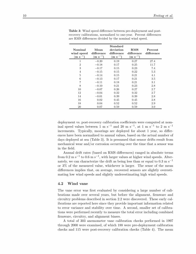
Table 3: Wind speed difference between pre-deployment and post-recovery calibrations, normalized to one-year. Percent differencesare RMS differences divided by the nominal wind speed.

StandardNominal Mean deviation RMS Percent

wind speed difference difference difference difference(m s−1) (m s−1) (m s−1) (m s−1)

1 −0.20 0.19 0.27 27.42 −0.18 0.17 0.25 11.73 −0.17 0.15 0.23 7.44 −0.15 0.15 0.22 5.35 −0.14 0.15 0.21 4.16 −0.13 0.17 0.21 3.57 −0.11 0.18 0.21 3.18 −0.10 0.21 0.23 2.8

10 −0.07 0.26 0.27 2.712 −0.04 0.32 0.32 2.714 −0.01 0.39 0.39 2.816 0.02 0.45 0.45 2.818 0.04 0.52 0.52 2.920 0.07 0.59 0.59 3.0

deployment vs. post-recovery calibration coefficients were computed at nom-inal speed values between 1 m s−1 and 20 m s−1, at 1 m s−1 to 2 m s−1

increments. Typically, moorings are deployed for about 1 year, so differ-ences have been normalized to annual values, based on the actual number ofdays deployed at sea (Table 3). It is presumed that sensor drifts result frommechanical wear and/or corrosion occurring over the time that a sensor wasin the field.

Annual drift rates (based on RMS differences) ranged in absolute termsfrom 0.2 m s−1 to 0.6 m s−1, with larger values at higher wind speeds. Alter-nately, we can characterize the drift as being less than or equal to 0.3 m s−1

or 3% of the measured value, whichever is larger. The sense of the meandifferences implies that, on average, recovered sensors are slightly overesti-mating low wind speeds and slightly underestimating high wind speeds.

4.2 Wind vane

The vane error was first evaluated by considering a large number of cali-brations made over several years, but before the alignment, firmware andcircuitry problems described in section 2.2 were discovered. These early cal-ibrations are reported here since they provide important information relatedto error variance and stability over time. A second, smaller set of calibra-tions were performed recently to measure the total error including combinedfirmware, circuitry, and alignment biases.

A total of 303 anemometer vane calibration checks performed in 1997through 2000 were examined, of which 188 were pre-deployment calibrationchecks and 115 were post-recovery calibration checks (Table 4). The mean


Table 4: Vane calibration error statistics for calibration checksmade before firmware, circuitry, and alignment errors were discov-ered. N is the number of instruments calibrated. Negative valuesimply that measured orientation is clockwise, or to the right, of thetrue orientation.

StandardType N Minimum Maximum mean Deviation RMS

(deg.) (deg.) (deg.) (deg.) (deg.)

Pre-deployment 188 –5.7 5.8 −0.28 1.13 1.16Post-recovery 115 −22.5 14.0 −1.01 3.19 3.23All 303 −22.5 14.0 −0.56 2.14 2.19

error was small (−0.28) for pre-deployment calibration checks, and onlyslightly larger (−1.01) for post-recovery calibration checks. Thus the meanerror did not change appreciably during deployment. Since mean errors weresmall, standard deviation and RMS error were nearly the same. The errorstandard deviation was 1.13 for pre-deployment calibration checks with arange of maximum errors of about ±6. As would be expected, errors werelarger for recovered sensors, with an error standard deviation of 3.19 andrange from −22 to +14. The error standard deviation was 2.14 for thecombined set of pre-deployment and post-recovery instruments.

The location of the wind vane dead zone was also checked before deploy-ment and after recovery of the sensors. The values presented here (Table 5)have been adjusted to reflect the alignment bias described in section 2.2.On average, the width of the dead zone was 3.9 for both pre-deploymentand post-recovery checks, compared to a nominal value of 5 as specified bythe manufacturer. The location of the dead zone typically rotated counter-clockwise about 1 during deployment, which is consistent with the changein mean error in Table 4.

When in the dead zone, the vane orientation is reported as 0. Therefore,on average, errors when in the dead zone would range from about −1 to+3 at deployment and about ±2 at recovery. These values are comparablein magnitude to ensemble errors outside the dead zone (given in Table 4).

Once the errors due to firmware, circuitry, and alignment errors werediscovered, we checked 23 vanes by recording their digitized output with thealignment correctly measured. Of these, 21 had not been used in the field,and two had been used for a 2-month long test on land at the Woods Hole

Table 5: Average location of the vane dead zone. N is the numberof instruments tested.

Type N Start End Width(deg.) (deg.) (deg.)

Pre-deployment 188 359.1 3.0 3.9Post-recovery 115 358.2 2.1 3.9All 303 358.8 2.7 3.9

12 Freitag et al.

Table 6: Vane calibration error statistics for calibration checksmade after measurement errors were discovered. N is the numberof instruments calibrated. Negative values imply that measuredorientation is counterclockwise, or to the left, of the true orienta-tion.

StandardType N Minimum Maximum Mean deviation RMS


Uncorrected 23 0.0 10.8 −6.8 2.0 7.1Corrected for alignment 10 −0.9 9.8 −4.1 2.2 4.6Corrected for alignment, firmware,

and circuitry20 −2.3 5.6 −1.0 1.3 1.6

Oceanographic Institution, near the seashore. The mean error for these vanesis clearly larger than that presented in Table 4 and is a better indicationof true mean error characteristics. The mean error was −6.8 (Table 6),the sign of which implies that vane readings were biased in the counterclockwise direction. For example, if the reported direction was 90, the truedirection would have been 96.8. The error standard deviation was 2.0, only1 larger than the error standard deviation for pre-deployment calibrationchecks made previously (Table 4). This suggests that the combined firmware,circuitry, and misalignment errors can be characterized mainly as a meanbias.

Beginning in fall 2000 the vane alignment method, firmware, and cir-cuitry were modified to improve the accuracy of the vane measurement.First, ten vanes were realigned and checked with the original firmware andcircuitry. Compared to the uncorrected vanes, the mean and RMS error ofthis group decreased by 2.7 and 2.5, respectively. Four anemometers fromthis group were deployed on moorings in October–November 2000. Soon af-ter, a group of 20 vanes were evaluated using corrected alignment, firmwareand circuitry. These modifications reduced the mean error for the ensem-ble to 1.0 and the RMS error to 1.6, values that are comparable to theresolution (1.4) of the digitization circuitry. Most moorings deployed inNovember 2000 and all moorings deployed thereafter had or will have vanescorrected for alignment, firmware, and circuitry.

4.3 Compass

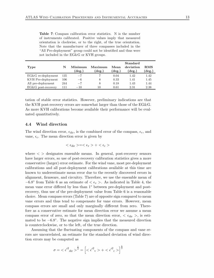
A total of 355 compass calibrations performed in 1997 through 1999 wereexamined. Of these 244 were pre-deployment calibrations and 111 were post-recovery calibration tests. Pre-deployment calibrations for the two types ofcompass were similar with an overall RMS error of 1.44 for 244 calibrations(Table 7).

The RMS error for 111 EG&G post-recovery calibration tests was 2.38.Note that while the mean error is small (0.61), its sign is opposite to themean vane error in Table 6. At the time of this analysis the number ofrecovered KVH compasses was much smaller and did not allow the compu-


Table 7: Compass calibration error statistics. N is the numberof instruments calibrated. Positive values imply that measuredorientation is clockwise, or to the right, of the true orientation.Note that the manufacturer of three compasses included in the“All Pre-deployment” group could not be identified and thus werenot included in the EG&G or KVH groups.

StandardType N Minimum Maximum Mean deviation RMS


EG&G re-deployment 135 −7 7 0.04 1.42 1.42KVH Pre-deployment 106 −6 8 0.33 1.41 1.45All pre-deployment 244 −7 8 0.18 1.43 1.44EG&G post-recovery 111 −10 10 0.61 2.31 2.38

tation of stable error statistics. However, preliminary indications are thatthe KVH post-recovery errors are somewhat larger than those of the EG&G.As more KVH calibrations become available their performance will be eval-uated quantitatively.

4.4 Wind direction

The wind direction error, εdir, is the combined error of the compass, εv, andvane, εc. The mean direction error is given by

< εdir >=< εv > + < εc >

where < > designates ensemble means. In general, post-recovery sensorshave larger errors, so use of post-recovery calibration statistics gives a moreconservative (larger) error estimate. For the wind vane, most pre-deploymentcalibrations and all post-deployment calibrations available at this time areknown to underestimate mean error due to the recently discovered errors inalignment, firmware, and circuitry. Therefore, we use the ensemble mean of−6.8 from Table 6 as an estimate of < εv >. As indicated in Table 4, themean vane error differed by less than 1 between pre-deployment and post-recovery, thus use of the pre-deployment value from Table 6 is a reasonablechoice. Mean compass errors (Table 7) are of opposite sign compared to meanvane errors and thus tend to compensate for vane errors. However, meancompass errors are small and only marginally different from zero. There-fore as a conservative estimate for mean direction error we assume a meancompass error of zero, so that the mean direction error, < εdir >, is esti-mated to be −6.8. The negative sign implies that the measured directionis counterclockwise, or to the left, of the true direction.

Assuming that the fluctuating components of the compass and vane er-rors are uncorrelated, an estimate for the standard deviation of wind direc-tion errors may be computed as

σ = < ε′2dir >12 =

[< ε′2v > + < ε′2c >

] 12

14 Freitag et al.

where < ε′2v > is the standard deviation of the vane errors about its mean,and < ε′2c > is the standard deviation of the compass errors about its mean.

A conservative estimate is obtained by using post-recovery values since,at the beginning of a deployment and for some time thereafter, errors wouldbe smaller. Thus, we use 3.2 as the standard deviation for vane errors(Table 4) and 2.3 as the standard deviation of compass errors. This leadsto an overall standard deviation of direction errors of 3.9. Combining themean and fluctuating components of the wind direction error then gives aconservative estimate of total direction error of

RMS Wind Direction Error = ((6.8)2 + (3.9)2)12 = 7.8

As noted in section 3.2, most sensors deployed in November 2000 and allthereafter have improved vane alignment, firmware, and circuitry. Initialcalibrations of these modified systems indicate that post-recovery RMS vaneerrors should be reduced to around 3 with little or no mean bias. In thefuture, therefore, we expect that wind direction errors will be around 5 orless.

5. Summary

The RMS error estimate for wind speed measured on Standard and NextGeneration ATLAS moorings was found to be less than or equal to 0.3 ms−1 or 3% of the speed, whichever is greater. This is a conservative estimateof overall instrumental error, as it was based upon the sensors’ recoveredstate. When first deployed, the RMS error is estimated to be 0.14 m s−1

over wind speeds from 1 m s−1 to 20 m s−1.The RMS error estimate for ATLAS mooring wind direction was found

to be 7.8, most of which was due to a mean wind direction error of –6.8

(counterclockwise, or to the left, of the true direction). This bias was pri-marily due to a misalignment of the vane and a bias in the vane digitizationfirmware and circuitry. Calibration procedures and firmware versions havechanged with time since the first ATLAS mooring was deployed in 1984.However, we believe that some mean direction bias has been present in themajority of historical ATLAS data, even though the time history of the erroris not exactly known. Given the uncertainty in mean bias for older data, nocorrection will be made to archived data from Standard ATLAS systems.

On the other hand, calibration procedures and firmware versions forNext Generation ATLAS systems have been consistent with regard to vaneprocessing. For this reason we plan to apply a mean direction correctionto all data from Next Generation moorings. These moorings began enter-ing the TAO Array in 1996 and will comprise 100% of the array after fall2001. All moorings in PIRATA have been Next Generation systems. The6.8 correction to be applied (Table 6) will be a significant improvement todata obtained from systems deployed before new alignment procedures andfirmware were developed. It is estimated that the new alignment proceduresand firmware will essentially eliminate the directional bias and lower RMSwind direction errors to about 5 or less in future deployments.


Direction bias between buoy winds and NSCAT satellite observationshave been reported to be of order 8 (Dickinson et al., 2001; Wentz andSmith, 1999). This bias is of similar magnitude and sign as that found inthis study, indicating that a significant amount of the satellite-buoy biasreported previously may be due to the vane errors reported here. To ourknowledge, however, no scientific study has been compromised as a result ofbiases in ATLAS wind directions.

6. Acknowledgments

We would like to thank Pat McLain of PMEL, who designed the ATLASelectronics and firmware and provided the authors with valuable details andinsights into their operation. This work was supported by NOAA’s Officeof Oceanic and Atmospheric Research, and by the Joint Institute for theStudy of the Atmosphere and Ocean (JISAO) under NOAA CooperativeAgreement #NA67RJO155.

7. References

Anonymous (1980): Handbook of magnetic compass adjustment. Defense MappingAgency Pub. No. 226, 96 pp.

Dickinson, S., K.A. Kelly, M.J. Caruso, and M.J. McPhaden (2001): A note on com-parisons between TAO buoy and NASA scatterometer wind vectors. J. Atmos.Oceanic Tech., 18, 799–806.

Freitag, H.P., Y. Feng, L.J. Mangum, M.P. McPhaden, J. Neander, and L.D. Strat-ton (1994): Calibration procedures and instrumental accuracy estimates ofTAO temperature, relative humidity and radiation measurements. NOAA Tech.Memo. ERL PMEL-104, 32 pp.

Hayes, S.P., L.J. Mangum, J. Picaut, A. Sumi, and K. Takeuchi (1991): TOGA-TAO: A moored array for real-time measurements in the tropical Pacific Ocean.Bull. Am. Meteorol. Soc., 72, 339–347.

McPhaden, M.J., A.J. Busalacchi, R. Cheney, J.R. Donguy, K.S. Gage, D. Halpern,M. Ji, P. Julian, G. Meyers, G.T. Mitchum, P.P. Niiler, J. Picaut, R.W.Reynolds, N. Smith, and K. Takeuchi (1998): The Tropical Ocean-Global At-mosphere (TOGA) observing system: A decade of progress. J. Geophys. Res.,103, 14,169–14,240.

Servain, J., A.J. Busalacchi, M.J. McPhaden, A.D. Moura, G. Reverdin, M. Vianna,and S.E. Zebiak (1998): A Pilot Research Moored Array in the Tropical Atlantic(PIRATA). Bull. Am. Meteorol. Soc., 79, 2019–2031.

Watson, J.D. (1992): Fluxgate compass limitations at high magnetic latitudes.APL-US Tech. Memo. TM 8-92, 34 pp.

Wentz, F.J., and D.K. Smith (1999): A model function for the ocean-normalizedradar cross section at 14 GHz derived from NSCAT observations. J. Geophys.Res., 104, 11,499–11,514.

16 Freitag et al.

Appendix A: Sample wind speed calibration

The results of a wind speed calibration of a TAO anemometer. A0 and A1are the calibration coefficients computed from a linear least-squares fit ofthe sensor output (counts) to the wind tunnel speed reported by a standardanemometer. Units (other than the sensor counts) are m s−1.

Sensor serial number: 28510

A0 = 2.3924703e-01A1 = 1.8729044e-01

Tunnel SensorCounts Speed Speed Residual

5.734 1.439 1.313 0.12611.941 2.402 2.476 -0.07321.311 4.188 4.231 -0.04232.983 6.415 6.417 -0.00241.095 7.951 7.936 0.01554.896 10.477 10.521 -0.04475.747 14.401 14.426 -0.025

104.812 19.916 19.870 0.046

MAXIMUM RESIDUAL = 0.1257


Appendix B: Sample wind vane calibration check

In the upper half of the form the sensor output (volts) is checked at 15

increments as recovered after use. In the lower half the sensor is recheckedafter replacement and reorientation of the potentiometer. The location ofthe potentiometer dead zone is also measured.

18 Freitag et al.

Appendix C: Sample compass calibration

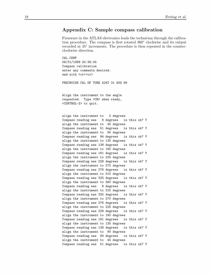
Firmware in the ATLAS electronics leads the technician through the calibra-tion procedure. The compass is first rotated 360 clockwise and its outputrecorded at 45 increments. The procedure is then repeated in the counter-clockwise direction.

CAL.COMP08/31/1999 20:36:04Compass calibrationenter any comments desired.end with <cr><cr>

PRECRUISE CAL OF TUBE 424T 31 AUG 99

Align the instrument to the anglerequested. Type <CR> when ready,<CONTROL-Z> to quit.

align the instrument to 0 degreesCompass reading was 8 degrees is this ok? Yalign the instrument to 45 degreesCompass reading was 51 degrees is this ok? Yalign the instrument to 90 degreesCompass reading was 94 degrees is this ok? Yalign the instrument to 135 degreesCompass reading was 138 degrees is this ok? Yalign the instrument to 180 degreesCompass reading was 181 degrees is this ok? Yalign the instrument to 225 degreesCompass reading was 228 degrees is this ok? Yalign the instrument to 270 degreesCompass reading was 276 degrees is this ok? Yalign the instrument to 315 degreesCompass reading was 325 degrees is this ok? Yalign the instrument to 360 degreesCompass reading was 8 degrees is this ok? Yalign the instrument to 315 degreesCompass reading was 325 degrees is this ok? Yalign the instrument to 270 degreesCompass reading was 276 degrees is this ok? Yalign the instrument to 225 degreesCompass reading was 228 degrees is this ok? Yalign the instrument to 180 degreesCompass reading was 181 degrees is this ok? Yalign the instrument to 135 degreesCompass reading was 136 degrees is this ok? Yalign the instrument to 90 degreesCompass reading was 94 degrees is this ok? Yalign the instrument to 45 degreesCompass reading was 51 degrees is this ok? Y


Next the firmware calculates a table of corrected compass values for eachof the 256 possible raw compass output values. This table is stored onboardthe instrument and corrects the compass in real time. The coefficients, P0through P4 may be used to rebuild the table, should it be corrupted in thefirmware.

Calculating table...P0= -312P1= 50P2= -100P3= 50P4= 75

0 1 2 3 4 5 6 7 8 9 A B C D E FF10000 FD FD FF 00 01 02 03 04 05 06 07 08 09 0A 0B 0CF10010 0D 0E 0F 10 11 12 13 14 15 16 17 18 19 1A 1B 1CF10020 1D 1E 1F 20 21 22 23 24 25 26 27 28 29 2A 2B 2CF10030 2D 2E 2F 30 31 32 33 34 35 36 37 38 39 3A 3B 3CF10040 3D 3E 3F 40 41 42 43 44 45 46 47 48 49 4A 4B 4CF10050 4D 4E 4F 50 51 52 53 54 55 56 57 58 59 5A 5B 5CF10060 5D 5E 60 61 62 63 64 65 66 67 68 69 6A 6B 6C 6DF10070 6E 6F 70 71 72 73 74 75 76 77 78 7A 7B 7C 7D 7EF10080 7F 80 81 82 83 84 85 86 87 88 89 8A 8B 8C 8D 8EF10090 8E 8F 90 91 92 93 94 95 96 97 98 99 9A 9B 9C 9DF100A0 9E 9F A0 A1 A1 A2 A3 A4 A5 A6 A7 A8 A9 AA AB ACF100B0 AD AE AE AF B0 B1 B2 B3 B4 B5 B6 B7 B8 B9 BA BBF100C0 BC BD BE BE BF C0 C1 C2 C3 C4 C5 C6 C7 C8 C9 CAF100D0 CB CC CD CE CF D0 D1 D2 D3 D4 D5 D6 D7 D8 D9 DAF100E0 DB DC DD DE DF E0 E2 E3 E4 E5 E6 E7 E8 E9 EA EBF100F0 EC ED EE EF F0 F1 F2 F3 F4 F5 F6 F7 F8 FA FB FCF10100 08 31 19 99 00 00 7F 69 FF FF FF FF FF FF FF FF

20 Freitag et al.

The compass is rotated again. This time the corrected compass output isrecorded at 15 increments. Angles are computed from the compass output(counts) by application of the factor 360/256.

do you want a cal test? Y08/31/1999 20:39: 27Compass calibrationenter any comments desired.end with <cr><cr>

TEST 424 31 AUG 99

Enter the test angle value, then <enter>.The system will respond with the calibratedvalue for that angle.TO QUIT enter an angle value of 999.

TEST ANGLE CORRECTED ANGLE RAW ANGLE CORRECTED CNTS RAW CNTS0 4 8 3 6

15 18 23 13 1630 32 37 23 2645 46 51 33 3660 60 65 43 4675 76 80 54 5790 89 93 63 66

105 104 108 74 77120 120 124 85 88135 135 138 96 98150 149 152 106 108165 163 166 116 118180 180 181 128 129195 195 197 139 140210 210 212 149 151225 225 228 160 162240 239 243 170 173255 255 260 181 185270 270 277 192 197285 285 293 203 208300 301 308 214 219315 319 325 227 231330 335 340 238 242345 349 354 248 252360 4 8 3 6999

done testing

calibration procedures and instrumental accuracies for ... · pdf filecalibration procedures...

Documents