calibration-constrained monte carlo uncertainty analysis ... · 2018. calibration-constrained monte...

GNS Science Consultancy Report 2017/219 March 2018

Calibration-constrained Monte Carlo uncertainty analysis of groundwater flow and contaminant transport models of the Heretaunga Plains

MJ Knowling P Rakowski

K Hayley BJC Hemmings

CR Moore

Project Number 630W0315-00

M.J. Knowling, GNS Science, Lower Hutt, New Zealand.K. Hayley, Groundwater Solutions Pty Ltd, Melbourne, Australia.C.R. Moore, GNS Science, Lower Hutt, New Zealand.P. Rakowski, Hawke’s Bay Regional Council, Napier, New Zealand.B.J.C. Hemmings, GNS Science, Lower Hutt, New Zealand.

DISCLAIMER

This report has been prepared by the Institute of Geological and Nuclear Sciences Limited (GNS Science) exclusively for and under contract to Hawke’s Bay Regional Council. Unless otherwise agreed in writing by GNS Science, GNS Science accepts no responsibility for any use of or reliance on any contents of this report by any person other than Hawke’s Bay Regional Council and shall not be liable to any person other than Hawke’s Bay Regional Council, on any ground, for any loss, damage or expense arising from such use or reliance.

Use of Data:

Date that GNS Science can use associated data: March 2018

BIBLIOGRAPHIC REFERENCE

Knowling MJ, Hayley K, Moore CR, Rakowski P, Hemmings BJC. 2018. Calibration-constrained Monte Carlo uncertainty analysis of groundwater flow and contaminant transport models of the Heretaunga Plains. Lower Hutt (NZ): GNS Science. 320 p. (GNS Science consultancy report; 2017/219).

Confidential 2018

GNS Science Consultancy Report 2017/219 i

CONTENTS

EXECUTIVE SUMMARY .............................................................................................. III

1.0 INTRODUCTION ............................................................................................... 1

2.0 THE GROUNDWATER MODELS ...................................................................... 2

2.1 EXISTING CALIBRATED FLOW MODEL AND SIMULATIONS ............................... 2 2.2 PARTICLE TRACKING MODEL AND MRT SIMULATIONS ................................... 3 2.3 NITRATE TRANSPORT MODEL AND “WORST CASE” PREDICTIVE SIMULATIONS . 4

3.0 CALIBRATION-CONSTRAINED MONTE CARLO ANALYSIS ......................... 6

3.1 LINEAR-ASSISTED MONTE CARLO .............................................................. 6 3.2 WORKFLOW ............................................................................................. 7

3.2.1 Approximate posterior (parameter) probability distribution ..................... 7 3.2.2 Monte Carlo analysis ............................................................................... 8 3.2.2.1. Sampling from C’(k) ................................................................................ 8 3.2.2.2. Re-calibration ......................................................................................... 8 3.2.2.3. Filtering ................................................................................................... 9 3.2.2.4. Uncertainty propagation ....................................................................... 10

3.3 HIGH PERFORMANCE COMPUTING RESOURCES ......................................... 10

4.0 RESULTS ........................................................................................................ 11

4.1 POSTERIOR PARAMETER PROBABILITY DISTRIBUTIONS .............................. 11 4.2 MODEL-TO-MEASUREMENT MISFIT ........................................................... 11

4.2.1 First filter: Φm1 ........................................................................................ 11 4.2.2 Second filter: Φm2 .................................................................................. 13 4.2.3 MRT misfit ............................................................................................. 15

4.3 DEMONSTRATION OF PARAMETER VARIABILITY AMONG CALIBRATED REALISATIONS ........................................................................................ 16

4.4 UNCERTAINTY OF “WORST-CASE” GROUNDWATER NITRATE DISTRIBUTION .. 16

5.0 DISCUSSION AND RECOMMENDATIONS .................................................... 17

6.0 REFERENCES ................................................................................................ 20

FIGURES

Figure 2.1 Pre-calibration scatterplot of simulated versus MRT estimates. ....................................... 4 Figure 4.1 Histogram of pre- and post-re-calibration (log-transformed) Φm1 among the 1,000

realisations. Four-hundred-and-sixty-two (462) of the realisations following re-calibration (orange) were deemed “acceptable” or “calibrated” on the basis of the first filter. .......... 12

Figure 4.2 Boxplot of observation group-based contributions to (log-transformed) Φm1 among the 362 acceptable realisations (blue) and the 578 non-acceptable realisations (red). ............... 13

Figure 4.3 Histogram of (log-transformed) Φm2 among the 362 realisations deemed to be acceptable following the first filter. One-hundred-and-seven (107) of the realisations were deemed “acceptable” or “calibrated” on the basis of the second filter. ......................................... 14

Confidential 2018

ii GNS Science Consultancy Report 2017/219

Figure 4.4 Boxplot of spring discharge observation group contributions to (log-transformed) Φm2 among the 107 realisations satisfying filter two (blue) versus those that satisfy filter one but not two (red). ............................................................................................................ 15

Figure 4.5 Boxplot of the mean-residence-time (MRT) observation-group contribution to (log-transformed) Φm (ΦMRT) among the (107) acceptable realisations. The base-calibrated model ΦMRT is shown by the black marker. .................................................................... 16

TABLES

Table 3.1 Modified PEST variables. ................................................................................................. 8

APPENDICES

A1.0 APPENDIX A: PRIOR PARAMETER UNCERTAINTY STANDARD DEVIATION ........................................................................................................... 24

A2.0 APPENDIX B: PRIOR AND POSTERIOR PROBABILITY DISTRIBUTIONS FOR MODEL PARAMETERS ............................................................ 25

A3.0 APPENDIX C: DEMONSTRATION OF PARAMETER VARIABILITY AMONG CALIBRATED REALISATIONS ....................................................... 183

A4.0 APPENDIX D: SIMULATED “WORST-CASE” GROUNDWATER NITRATE CONCENTRATIONS AMONG CALIBRATED MODEL REALISATIONS ............................................................................... 211

APPENDIX FIGURES

Figure A2.1 Prior and posterior parameter probability distributions. .................................................. 25 Figure A3.1 Horizontal aquifer hydraulic conductivity for each model layer (1-2; left and middle,

respectively) and riverbed conductance (right) for each of the 107 calibrated model realisations (7-1000) (1 rows per realisation). Consistent colour bars are used for reference. ..................................................................................................................... 183

Figure A4.1 Simulated “worst-case” nitrate concentration distributions for each model layer (1-6) for each of the 107 calibrated model realisations (indexed 7-1000) (2 rows per realisation; 2 realisations per page). A consistent colour bar, spanning from 0.0 to 20.0 mg/L (the maximum simulated nitrate concentration occurring across all realisations) is used for reference. ..................................................................................................................... 211

Figure A4.2 Simulated “worst-case” (log10-transformed) nitrate concentration distributions for each model layer (1-6) for each of the 107 calibrated model realisations (indexed 7-1000) (2 rows per realisation; 2 realisations per page). A consistent colour bar, spanning from -2 to 2.1 log-N mg/L, is used for reference. .......................................................................... 266

APPENDIX TABLES

Table A1.1 Group-based prior parameter uncertainty standard deviations. ...................................... 24

Confidential 2018

GNS Science Consultancy Report 2017/219 iii

EXECUTIVE SUMMARY

This report summarises the outcomes of a formal uncertainty analysis of groundwater flow and contaminant transport models of the Heretaunga Plains aquifer system (Hawke’s Bay, New Zealand). The objective of this work is to produce a suite of calibration-constrained groundwater model parameter realisations that can be used collectively for the purposes of quantifying the uncertainty surrounding model parameters and predictions of management interest made on the basis of these model parameter realisations. This work contributes to the development of decision support, incorporating risk assessment, for water- and land-use management in the Heretaunga Plains. The analyses described in this report complement a number of groundwater science investigations toward sustainable water resource management within the Tutaekuri, Ahuriri, Ngaruroro and Karamu catchments, which are hydrologically connected via the Heretaunga Plains aquifers.

A calibration-constrained non-linear uncertainty quantification methodology was employed for the analyses described in this report. The method, referred to as “linear-assisted Monte Carlo” or LAMC, involves the propagation of a Bayesian linear approximation to the posterior parameter probability distribution (Doherty, 2015). Application of this method ultimately results in the development of a suite of “calibrated” model parameter realisations. Each of these “calibrated” parameter realisations produce satisfactory matches to field observation data, while differing in parameter values that are not well informed (but may be important in the context of making predictions). Differences among these parameter realisations occur as a result of parameter non-uniqueness, which is caused by a combination of parameter correlation, data scarcity and measurement uncertainty. Predictions of management interest in the Heretaunga Plains, e.g., nitrate concentrations, can then be simulated on the basis of all of these parameter realisations, thus allowing for the uncertainty surrounding these predictions to be expressed in a probabilistic fashion. The analysis takes into account the uncertainty associated with the following sources:

• Non-uniqueness in calibrated flow-model parameter values (e.g., rainfall recharge and irrigation-well pumping rate multipliers, drain conductance, etc.) and distributions (e.g., hydraulic conductivity, river-bed conductance, aquifer storativity, etc.);

• Measurement error associated with groundwater-level observations, surface water-groundwater exchange estimates, etc.;

• Effective aquifer porosity and its spatial variability; and

• Nitrate concentration in rainfall recharge (or “load”) and river recharge and their spatial variabilities.

Generally, the posterior parameter probability distributions displayed only subtle changes relative to the prior probability distributions (i.e., prior to history matching). This indicates a generally low ability to uniquely estimate these model parameters based on the (relatively sparse) information content of the calibration dataset. Parameters displaying the largest degree of constraint (i.e., narrowing and heightening of the probability distributions) through history matching are generally those that aggregate model quantities over large spatial (or temporal) scales, as expected.

Following parameter upgrading for each realisation on the basis of the existing “calibrated” Jacobian matrix (i.e., a sort-of “re-calibration”), and a two-stage “filtering” process (i.e., removing model realisations that produce poor model-to-measurement fit), a total of 107 “calibrated” parameter realisations were obtained from some 1,000 prior (i.e., unconstrained) parameter realisations. These realisations collectively display vast differences in parameter values, in

Confidential 2018

iv GNS Science Consultancy Report 2017/219

particular for spatially distributed aquifer parameter values that are poorly informed by field observations (e.g., aquifer hydraulic conductivity). The model outputs based on these 107 realisations all display an acceptable level of model-to-measurement misfit, on the basis of the overall objective function, and also reproduce a select number of important observation groups acceptably well. To the extent that a model prediction of interest is sensitive to parameters that display a large degree of uncertainty, the prediction will also be largely uncertain.

The uncertainty surrounding a “worst-case” nitrate concentration predictive scenario simulation (involving assumptions of steady-state and zero denitrification) was also explored using the parameter realisation suite. It was shown that, among the calibrated realisations, simulated nitrate concentrations display a significant degree of spatial variability. Despite the “worst case” nature of the predictive scenario, relatively low nitrate concentrations (e.g., <5 mg/L) were simulated to occur across large portions of the model domain among the model realisations, particularly in the plains and at depth. Localised nitrate concentrations that exceed the Ministry of Health’s (2008) drinking water guideline threshold value of 11.3 mg/L, were also simulated, generally occurring within the valley reaches of the model domain. These outcomes can be used to identify regions of nitrate-contamination susceptibility, e.g., vulnerability maps.

This work provides HBRC with the capability to conduct risk assessments associated with a wide variety of water- and land-use management predictive scenarios in the future. Such investigations have already begun. For example, the suite of calibrated parameter realisations presented here is currently being used to explore and map the vulnerability of streamflow to groundwater abstraction (White et al., in prep). The uncertainty of groundwater discharge rates at culturally and environmentally significant streams and springs within the area are also of significant interest, and are expected to be investigated in the future using the same suite of model parameter realisations produced as part of this work.

Confidential 2018

GNS Science Consultancy Report 2017/219 1

1.0 INTRODUCTION

Hawke’s Bay Regional Council (HBRC) commissioned GNS Science to undertake a formal model parameter and predictive uncertainty analysis for groundwater flow and contaminant transport models of the Heretaunga Plains aquifer system. This work complements previous and concurrent modelling work, including Rakowski and Knowling (in prep) and Anderson (2017), undertaken as part of a number of groundwater science investigations toward sustainable water resource management within the Tutaekuri, Ahuriri, Ngaruroro and Karamu catchments (TANK), which are hydrologically connected via the Heretaunga Plains aquifer system. The primary focus of previous and concurrent modelling has been to assess the impacts of water- and land-use allocation on surface and groundwater quality and quantity.

The models developed and applied prior to this work had not undergone uncertainty quantification analyses. This is a requirement for numerical models to be able to reliably and robustly support environmental management decision-making, i.e., from a risk-based perspective. Such analyses are therefore needed for the modelling carried out within the TANK investigations to support water and land-use management within the Hawke’s Bay region.

This study presents a calibration-constrained non-linear uncertainty analysis, using the flow and transport models developed previously, as well as various models developed as part of this study, together with existing historical hydrological data. The analysis methodology employed is considered to be the “best practice” approach within the groundwater modelling and management context (e.g., Australian Groundwater Modelling Guidelines; Barnett et al., 2012).

This study provides a numerically robust platform for improved groundwater quantity and quality management in the Heretaunga Plains. The primary output of this study is the suite of calibration-constrained groundwater model parameter realisations. Prediction uncertainty can be explored by running the predictive simulation model with each of these parameter realisations. This allows the risks associated with various scenarios and impact assessments to be explored, and some of these assessments are already underway (e.g., White et al., in prep).

Confidential 2018

2 GNS Science Consultancy Report 2017/219

2.0 THE GROUNDWATER MODELS

This study involves the quantification of the uncertainty associated with the parameters employed by three different groundwater flow and transport models. These three models were each deployed in various model simulations, for the calibration and predictive phases of the uncertainty analysis. The details of these models and model simulations are described below. The uncertainty analysis methodology workflow which combines these models is described in Section 3.2.

2.1 EXISTING CALIBRATED FLOW MODEL AND SIMULATIONS

A suite of nine different calibrated groundwater flow model simulations of the Heretaunga Plains, which represent different historical conditions and temporal discretisations, were considered within the calibration phase of the uncertainty analysis (Section 3.2.2.2). The reader is directed to Rakowski and Knowling (2017) for a detailed description of the development and calibration of the model and these simulations. They are as follows:

1. “HPM”. A steady-state model simulation representing contemporary climate and water-use conditions (time-averaged stresses between 2005 and 2015). This is used primarily for parameter estimation purposes.

2. “HPM_80”. A steady-state model simulation representing climate and water-use conditions during the 1980s (time averaged stresses between 1980 and 1989). This is used for providing initial conditions for “HPM_A”.

3. “HPM_6”. This is a six-layer equivalent to the (two-layer) HPM model. This alternative model structure is used for generating cell-by-cell flow budgets required for contaminant transport and particle tracking models.

4. “HPM_A”. An annual transient model simulation, spanning the period 1 July 1980–30 June 2015. This was used both for calibration purposes and for investigating long-term groundwater storage trends. It is also used for generating initial conditions for the following transient models.

5. “HPM_M1”. A monthly transient model simulation spanning the period 1 April 1997–31 March 1999 (when monthly water-level data are plentiful). This model simulation was used primarily for calibration purposes.

6. “HPM_M2”. A monthly transient model simulation spanning the period 1 April 2011–31 March 2015 (when monthly water-level data are plentiful). This model simulation was used primarily for calibration purposes.

7. “HPM_E1”. A 7-day transient model simulation representing flood-event conditions during the period starting on 25 May 2001.

8. “HPM_E2”. A 7-day transient model simulation representing flood-event conditions during the period starting on 20 September 2001.

9. “HPM_E3”. A 7-day transient model simulation representing flood-event conditions during the period starting on 20 September 2015.

A total of 1062 parameters (822 of which are adjustable) are linked to the flow model simulations described above. Parameter groups are given in Table A1 (Appendix A).

Two modifications to the existing flow-model parameterisation set-up were necessary during the course of the current work. They are as follows:

Confidential 2018


1. The use of the SCALE variable in PEST for the following nine parameters: “irng”; “rapr”; “karm”; “mngt”; “krwg”; “krwl”; “tt-w”; “qfac”; and “rch”. A SCALE value of 0.01 was adopted. This effectively means that the sensitivity of model outputs with respect to these parameters was reduced, which was necessary in mitigating non-credible posterior probability distributions, particularly for the parameters “qfac” and “rch”. The use of SCALE was found to be more effective than log-transforming these parameters in terms of the reasonableness of the resulting posterior probability distributions.

2. The removal of the "fixed” status of two of the specific yield pilot point parameters (“ppsy78” and “ppsy90”) that were used during the original model calibration. This was so that their uncertainties could be explored.

2.2 PARTICLE TRACKING MODEL AND MRT SIMULATIONS

To provide a basis for incorporating recent mean-residence time (MRT) estimates (Morgenstern et al., 2018) into the current project, a particle-tracking model was developed. This model provided a means by which MRT estimates could inform, through a partial model parameter calibration, aquifer effective porosity values and their spatial variability, which is otherwise uninformed by the other available observation data. This was achieved using the methodology discussed in Section 3.2.1, despite not being part of the initial model calibration effort described in Section 2.1. Effective porosity is parameterised using (235) pilot points. MRT estimates are also used to inform other aquifer parameters, e.g., hydraulic conductivity. The use of a particle-tracking model in this context should, however, be considered approximate due to its representation of advective transport processes only (i.e., diffusion, dispersion and retardation are neglected).

Reverse particle tracking simulations were performed using MODPATH (version 6; Pollock, 2012). The locations where MRT observations were made were correlated with model cells of the 6-layer flow model (HPM_6). For the MRT estimate locations within the model domain (of which there are 52), a 10 x 10 grid of particles was released on each face of the model cells associated with the observation well-screen location (600 particles each). The average simulated exit time of the 600 particles for each observation location was compared with the estimated MRT via calibration. A log-transformation was applied to both observation and simulation data to improve the performance of the calibration by linearising these quantities.

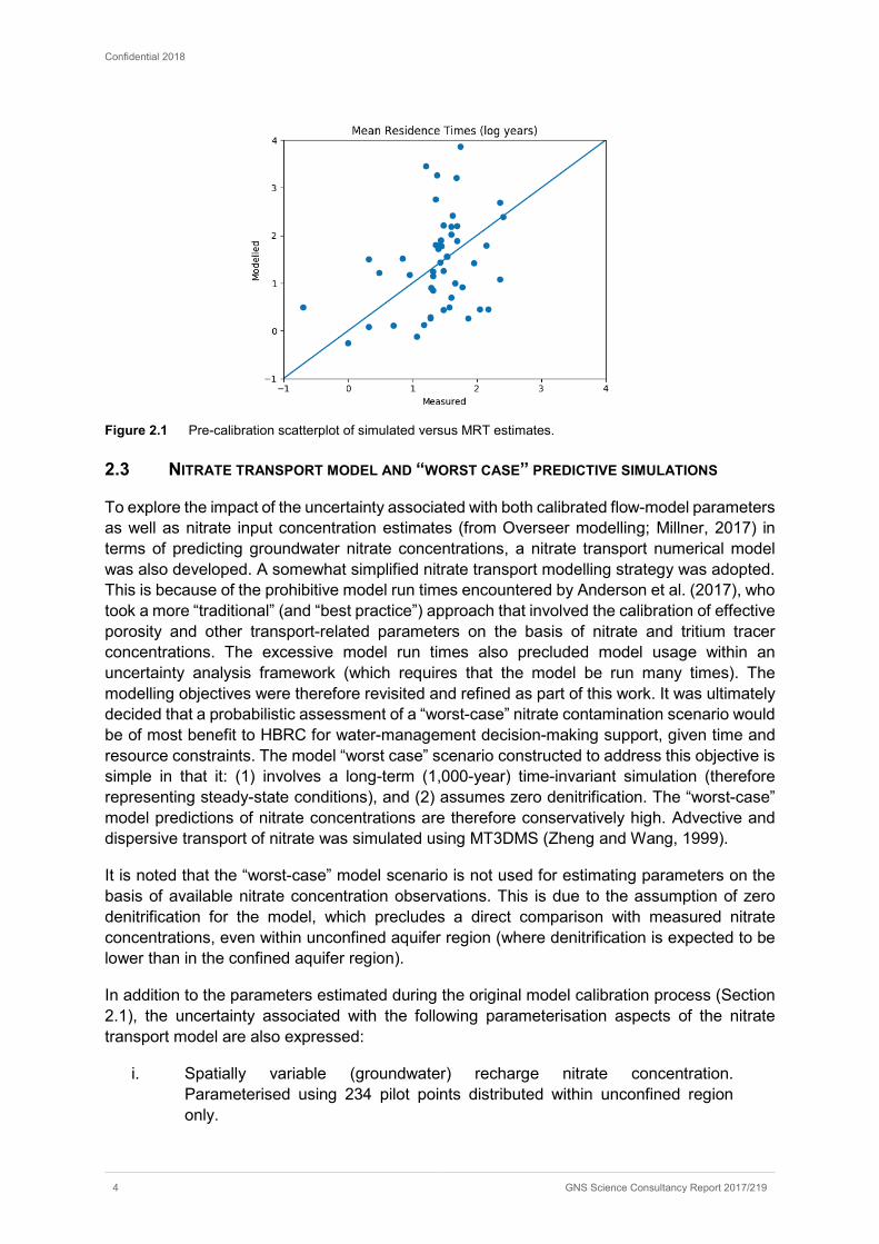
Figure 2.1 shows particle tracking results in terms of MRT based on the calibrated contemporary steady-state flow model (HPM) and a uniform effective aquifer porosity value of 0.1. While the assumption of a uniform porosity distribution is not appropriate, this case nevertheless represents an initial condition for the partial calibration which was undertaken (Section 3.2.1).

Confidential 2018


Figure 2.1 Pre-calibration scatterplot of simulated versus MRT estimates.

2.3 NITRATE TRANSPORT MODEL AND “WORST CASE” PREDICTIVE SIMULATIONS

To explore the impact of the uncertainty associated with both calibrated flow-model parameters as well as nitrate input concentration estimates (from Overseer modelling; Millner, 2017) in terms of predicting groundwater nitrate concentrations, a nitrate transport numerical model was also developed. A somewhat simplified nitrate transport modelling strategy was adopted. This is because of the prohibitive model run times encountered by Anderson et al. (2017), who took a more “traditional” (and “best practice”) approach that involved the calibration of effective porosity and other transport-related parameters on the basis of nitrate and tritium tracer concentrations. The excessive model run times also precluded model usage within an uncertainty analysis framework (which requires that the model be run many times). The modelling objectives were therefore revisited and refined as part of this work. It was ultimately decided that a probabilistic assessment of a “worst-case” nitrate contamination scenario would be of most benefit to HBRC for water-management decision-making support, given time and resource constraints. The model “worst case” scenario constructed to address this objective is simple in that it: (1) involves a long-term (1,000-year) time-invariant simulation (therefore representing steady-state conditions), and (2) assumes zero denitrification. The “worst-case” model predictions of nitrate concentrations are therefore conservatively high. Advective and dispersive transport of nitrate was simulated using MT3DMS (Zheng and Wang, 1999).

It is noted that the “worst-case” model scenario is not used for estimating parameters on the basis of available nitrate concentration observations. This is due to the assumption of zero denitrification for the model, which precludes a direct comparison with measured nitrate concentrations, even within unconfined aquifer region (where denitrification is expected to be lower than in the confined aquifer region).

In addition to the parameters estimated during the original model calibration process (Section 2.1), the uncertainty associated with the following parameterisation aspects of the nitrate transport model are also expressed:

i. Spatially variable (groundwater) recharge nitrate concentration. Parameterised using 234 pilot points distributed within unconfined region only.

Confidential 2018


ii. Spatially variable river nitrate concentration. Parameterised river reach-by-reach.

iii. Global dispersivity parameters (longitudinal, transverse-longitudinal ratio, vertical transverse-longitudinal ratio).

The prior uncertainty standard deviations associated with these parameters, supplied by HBRC, are given in Table A1.1 (Appendix A).

Confidential 2018


3.0 CALIBRATION-CONSTRAINED MONTE CARLO ANALYSIS

The industry-standard groundwater-model calibration and uncertainty analysis software PEST (Doherty, 2016) offers means by which calibration-constrained non-linear uncertainty quantification can be achieved in a computationally efficient manner (e.g., Tonkin and Doherty, 2009). It is worth noting that the approaches offered by PEST are unique and well-regarded within international scientific literature due to their efficiency in highly parameterised modelling contexts. High parameter dimensionality is often required when calibrating groundwater models, and when analysing predictive uncertainty. This is because groundwater observations and predictions such as groundwater levels, surface water- groundwater fluxes, and concentrations, are frequently sensitive to fine-scale system detail that cannot be represented with more lumped parameterisations.

Calibration-constrained Monte Carlo analyses ultimately produce a suite of model parameter realisations that are all considered to produce satisfactory matches to field observation data, yet differ where parameters are not well informed by the field observation data. Collectively, these model realisations provide an expression of model parameter uncertainty, and can be used to explore the uncertainty associated with model predictions. This constitutes probabilistic model usage.

3.1 LINEAR-ASSISTED MONTE CARLO

This study employs the “linear-assisted Monte Carlo” (LAMC) methodology (e.g., Doherty, 2015; Tarantola, 2005). The LAMC method involves the propagation of a linear approximation (also known as Schur’s complement; White et al., 2016) to the posterior parameter probability distribution. The use of the (albeit approximate) posterior probability distributions constitutes the calibration-constrained nature of this uncertainty method, as described above.

It is worth noting here the need to approximate the posterior parameter probability distribution in the context of complex and highly parameterised groundwater models. Purer (i.e., less approximate) means of determining the posterior probability distribution, such as Markov-chain Monte Carlo (e.g., Vrugt, 2016), involve significantly greater computational expense; these methods are therefore deemed inappropriate for the purposes of the current study.

The posterior covariance matrix of model parameters, C’(k), can be expressed via a linearised form of Bayes equation (Christensen and Doherty, 2008):

)()]()([)()()( 1 kXCεCXkXCXkCkCkC −+−=′ tt (3.1)

Where C(k) is the prior (i.e., pre-history matching) covariance matrix of k, and is user-specified based on expert knowledge pertaining to geological (or otherwise) site characteristics, X is a matrix that represents the action of a (linear) model (the tangential linear operator), C(ε) is the covariance matrix of epistemic noise (i.e., including effects of model structural errors and measurement errors) (often assumed to have non-zero diagonal elements only).

Equation 3.1 assumes a linear relation between model parameters and observations (i.e., the X matrix is independent of the parameter values k). It also assumes that parameter and epistemic error distributions are Gaussian. In as much as these assumptions hold, Monte Carlo sampling from the (approximated) posterior covariance matrix C’(k) should, theoretically, produce a range of model-to-measurement misfit statistics that are, on average, similar to that of the base calibrated model, and that span both above and below that of the base calibrated model objective function value. However, even slight nonlinearities in the inverse problem can

Confidential 2018


increase the model-to-measurement misfit for certain realisations. Therefore, to further reduce the model-to-measurement misfit, each model realisation may need to be subject to re-calibration (e.g., Herckenrath et al., 2011).

3.2 WORKFLOW

The LAMC methodology workflow adopted here involves a number of distinct steps. These are described below.

3.2.1 Approximate posterior (parameter) probability distribution

The approximation of C’(k) was carried out using the PREDUNC7 utility (Doherty, 2016). This required the specification of three matrices C(k), X and C(ε), as per Equation (3.1). This involved the following steps:

a. Populate C(k). The prior parameter covariance matrix C(k) was populated based on hydrological and geological expert knowledge. C(k) was assumed to be a diagonal matrix (i.e., C(k) does not contain off-diagonal elements). Note that this means that zero spatial correlation was assumed to exist between pilot points used to parameterised aquifer hydraulic property fields such as hydraulic conductivity, storage parameters, effective porosity, etc. This is regarded to be a conservative approach (in terms of parameter field reasonableness) given that assuming zero spatial correlation allows for more extreme contrasts within parameter fields. This approach is considered to be appropriate given both the limited spatial coverage of aquifer property information and the highly heterogeneous nature of the Heretaunga Plains aquifer sediments. The diagonal elements of C(k), i.e., the standard deviation of prior parameter uncertainty, were supplied by HBRC. These values are listed in Table A1.1.

b. Populate X. The Jacobian matrix X was computed with respect to the base calibrated model parameter values using one-percent (1%) two-point derivative increments. The PEST variable DERFORGIVE was enabled for this step. Parameter perturbations that cause model non-convergence are therefore assigned a sensitivity of zero in the Jacobian matrix, i.e., instead of PEST terminating. Regularisation constraints were then removed using the utilities SUBREG1 and subsequently JCO2JCO (Doherty, 2016) for the purposes of the ensuing analysis.

c. Populate C(ε). The covariance matrix of epistemic noise C(ε) (assumed to be diagonal) was specified in accordance with:

12)( −= QεC rσ (3.2) where Q is a matrix whose diagonal elements correspond to (the square of) observation weights, and σr

2 (a scalar) is the so-called “reference variance”. The Q matrix is specified here following use of the PWTADJ2 utility (Doherty, 2016). This sets observation weights in such a way that they are approximately inversely proportional to the standard deviation of epistemic uncertainty standard deviation. This approach results in a base calibration measurement objective function equal to the number of non-zero weighted observations, as each squared-weighted-residual contributes one to the objective function. This approach also preserved intra-group relative weighting, and generally caused only relatively minor adjustments to observation weighting (because the existing

Confidential 2018


weights were prescribed during the flow model calibration in such a way that reflects the confidence with which observations are considered). A reference variance value of 1.0 was assigned. This value is deemed to be conservative given that the suggested (albeit approximate) value equals 0.05 (based on the base-calibrated model measurement objective function divided by the number of non-zero weighted observations; Doherty, 2015). The value assigned is therefore expected to give rise to conservative uncertainty intervals, which is considered to be a desirable output from this first step within the LAMC methodology.

3.2.2 Monte Carlo analysis

The Monte Carlo-aspect of the analysis involves the following steps, described in detail below.

3.2.2.1. Sampling from C’(k)

The RANDPAR utility (Doherty, 2016) was used to generate parameter set realisations using a random number generator algorithm. One-thousand (1,000) realisations were generated. This number of realisations was sufficient to satisfy HBRC’s request for at least 100 calibration-constrained models. Gaussian probability distributions were assumed for all parameters or their log-10-transformations. The expected value was centred at the base calibrated model parameter value. The was necessary to achieve an adequate number of models that can be considered “calibrated”. Parameter-value bounds were respected in all cases.

3.2.2.2. Re-calibration

The models are then run with each of the RANDPAR-generated parameter-set realisations; however, unsurprisingly, the model outputs associated with these realisations generally displayed poor matches to observation data. A parameter upgrading step was therefore conducted for each of the model parameter realisations (this step is referred to herein as “re-calibration” for conciseness). Note that the observation weights used for the re-calibration step are those that were PWTADJ2-adjusted for the posterior parameter distribution approximation (Section 3.2.1). Parameter upgrade vectors were computed based on the previously established base-model “calibrated” Jacobian matrix only; i.e., a single “optimisation iteration” was run (the maximum number of iterations (NOPTMAX) was set to one). This allows for a reduction in model-to-measurement misfit at a relatively very small computational cost (Tonkin and Doherty, 2009). Table 3.1 below lists PEST variables specified that are relevant to the re-calibration step. The JACUPDATE setting of 999 means that the Broyden rank-one Jacobian-matrix update (e.g., Skahill et al., 2009) is undertaken after every parameter upgrade attempt. The JACUPDATE and PHIRATSUF variable settings effectively maximise the potential for reducing the objective function during the re-calibration step. During the re-calibration step, the ADDREG1 utility (Doherty, 2016) was used to impose Tikhonov regularisation constraints such that the deviation from sampled parameter values is limited to where it is necessary to achieve a fit with observation data.

Because not all model parameter realisations provided good model-to-measurement matches, even after the re-calibration step, additional filters were applied, as discussed below.

Table 3.1 Modified PEST variables.

PEST variable Current value

JACUPDATE 999

PHIREDLAM 0.01

Confidential 2018


FRACPHIM 0.0

3.2.2.3. Filtering

A two-stage “filtering” process (i.e., whereby a sub-set of model parameter realisations is derived following the rejection of those that produce poor model-to-measurement fit) was performed across all of the realisations. Filtering in such a way represents the basis for the widely applied Generalised Likelihood Uncertainty Estimation (GLUE) method (e.g., Beven and Binley, 1992). This approach was used in order to establish a set of model parameter realisations that are deemed to be “acceptable”, in terms of their model-to-measurement misfit. Model-to-measurement misfit is quantified in accordance with a least-squares weighted measurement objective function Φm. Note that the observation weights used for filtering are also those following PWTADJ2-adjustment (Section 3.2.1), and that this differs from that used in the original base model calibration. Φm is comprised up of multiple components, each of which represents the degree of misfit for a given observation type or group. These observation-groups include mean-in-time heads, temporal deviation-from-the-mean heads, vertical head differences, spring discharge rates during summer, spring discharge rates during winter, river-aquifer exchange fluxes, long-term transient head trend, and MRT estimates.

The two filters used for refining the model realisation suite are now described. The filtering process was performed and automated using Python scripts.

a. Filter One: All observation-group contributions to Φm except “springs_sum”, “springs_win” and “MRT”. Firstly, all observation group components of Φm except those pertaining to seasonal spring discharge measurements (“spring_sum” and “spring_win” observation groups) and MRT estimates (“MRT” observation group) were collated. The sum of the Φm contribution from these selected groups, expressed herein as Φm1, was then compared to that of the base calibrated model, for each model realisation. A threshold of 10% above the base-calibrated model Φm1 (6217.7 + 621.77 = 6839.52) was used to define a “acceptable level of misfit”, under which the models are deemed to be “calibrated”. This acceptable-misfit threshold was agreed between HBRC and GNS Science. “Filtered” (or “behavioural”) realisations, i.e., those meeting the above criterion were then tested against the second filter (see below). It is worth noting that the acceptance threshold of 10% above the base-model Φm1 represents the effect of not only measurement uncertainty, but also model structural errors; Doherty and Welter (2010); to this end, larger percentage thresholds have also been adopted by, e.g., Tonkin and Doherty (2009) and Herckenrath et al. (2011). This threshold could therefore be relaxed to achieve a large number of calibrated realisations for future studies.

b. Filter Two: Observation groups “springs_sum” and “springs_win” contributions to Φm. Secondly, the seasonal spring discharge-related observation group (“spring_sum” and “spring_win”) components of Φm were collated into a second filter (the sum of the Φm contribution from these two groups is expressed herein as Φm2). An assessment of absolute spring flow residuals for a number of realisations with different Φm2 values were used to identify an “acceptable” level of spring flow misfit. The Φm2 value threshold for defining this acceptable level was taken as 16,000 (note that this is significantly higher than the base-calibrated model Φm2 value of 63.0, for the reasons discussed in Section 4.2.2). This

Confidential 2018


threshold was agreed between HBRC and GNS Science. The larger threshold value applied here is to better reflect the uncertainty surrounding spring flow observations contained within these groups, particularly for low flow rates, as well as the relatively approximate model representation of springs compared to the complexity of a natural spring discharge process.

Note that MRT estimates were not used as a basis for filtering model realisations. This is because a minimised objective function for this observation group had not been previously established (i.e., these data were not previously calibrated to).

3.2.2.4. Uncertainty propagation

The predictive nitrate transport model was then run using each of the model parameter realisations that satisfy the filters (referred to herein as “acceptable” or “calibrated” realisations) (Section 3.2.2.3), plus the “un-calibrated” nitrate transport-related parameters (Section 2.3), to assess predictive uncertainty. All model output quantities of interest, as well as for the re-calibration step described above, are collected for each realisation using shell/bash scripts.

3.3 HIGH PERFORMANCE COMPUTING RESOURCES

All model runs conducted during the course of this work were performed using HBRC’s computing resource allocation on the New Zealand eScience Infrastructure’s (NeSI) “Pan” high-performance cluster. A total of approximately 100,000 processing hours were used.

Confidential 2018


4.0 RESULTS

4.1 POSTERIOR PARAMETER PROBABILITY DISTRIBUTIONS

Figure A2.1 (Appendix B) shows the sampled prior and posterior probability distributions for the 1,878 model parameters integrated within the PEST framework (1,640 of which are adjustable and not “tied” parameters). The prior probability distributions for each parameter (left) are governed solely by C(k), which is user-defined a priori. The mean of the probability distributions coincides with base calibrated model parameter values (Section 3.2.1). Note that for parameter values that have not been subject to estimation through calibration (e.g., effective porosity), the mean of the prior distribution is the midpoint between the user-specified upper and lower parameter bounds. The posterior probability distributions (right) is produced using Equation 3.1. As described, to the extent that a parameter is well-informed by field observations contained within the calibration dataset, the posterior probability distribution will be narrower and taller than that of the prior.

Figure A2.1 indicates that the vast majority of parameters display only subtle narrowing and heightening of the probability distribution through history matching. This is the case in particular for parameters representing relatively high-resolution parameter variability (e.g., aquifer conductivity parameters “ppkx168”-“ppkx181”, “ppkz1”-“ppkz81”, etc.). This indicates an inability to uniquely estimate model parameters based on the (relatively sparse) information content of the calibration dataset. However, some exceptions exist. For example, aquifer conductivity parameters “ppkx12”, “ppkx72, “ppkx214”, and “ppkz282” display considerable difference between the prior and posterior distributions; this is due to the spatially localised nature of the information contained within field observations of, e.g., groundwater-levels. Parameters displaying a larger degree of constraint through history matching are generally those that aggregate model quantities over larger spatial (or temporal) scales (e.g., “qfac”, “rch”, “dr0”, “rv13”, and “irng”). This is because these large-scale parameters are informed by a relatively large number of observations.

4.2 MODEL-TO-MEASUREMENT MISFIT

4.2.1 First filter: Φm1

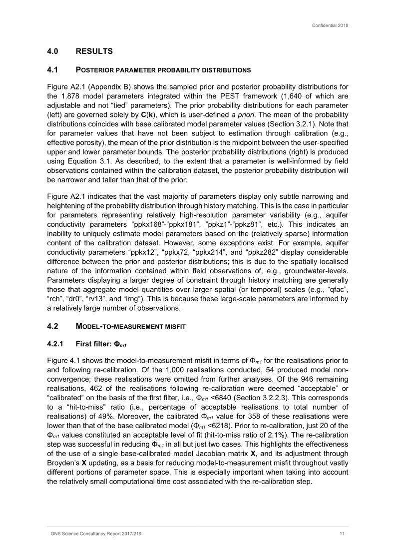
Figure 4.1 shows the model-to-measurement misfit in terms of Φm1 for the realisations prior to and following re-calibration. Of the 1,000 realisations conducted, 54 produced model non-convergence; these realisations were omitted from further analyses. Of the 946 remaining realisations, 462 of the realisations following re-calibration were deemed “acceptable” or “calibrated” on the basis of the first filter, i.e., Φm1 <6840 (Section 3.2.2.3). This corresponds to a “hit-to-miss" ratio (i.e., percentage of acceptable realisations to total number of realisations) of 49%. Moreover, the calibrated Φm1 value for 358 of these realisations were lower than that of the base calibrated model (Φm1 <6218). Prior to re-calibration, just 20 of the Φm1 values constituted an acceptable level of fit (hit-to-miss ratio of 2.1%). The re-calibration step was successful in reducing Φm1 in all but just two cases. This highlights the effectiveness of the use of a single base-calibrated model Jacobian matrix X, and its adjustment through Broyden’s X updating, as a basis for reducing model-to-measurement misfit throughout vastly different portions of parameter space. This is especially important when taking into account the relatively small computational time cost associated with the re-calibration step.

Confidential 2018


Figure 4.1 Histogram of pre- and post-re-calibration (log-transformed) Φm1 among the 1,000 realisations. Four-hundred-and-sixty-two (462) of the realisations following re-calibration (orange) were deemed “acceptable” or “calibrated” on the basis of the first filter.

Figure 4.2 shows the contribution to Φm1 from various observation groups for both the 462 “calibrated” models (on the basis of the first filter) and the remaining 484 realisations. Φm1 contributions among the acceptable models (shown in blue) are generally lower across the observation groups. Observation groups “ar_diff_2”, “h_diff_3”, “h_tr_a”, “h_tr_1”, “h_tr_2”, “trend_1” and “trend_2” display relatively consistent Φm1 contributions among all realisations. This suggests that the model outputs related to these groups are relatively insensitive to the sources of uncertainty expressed in the model and accompanying observations. For example, for observation groups representing deviation-from-the-mean monthly head variability (“h_tr_m1” and “h_tr_m2”), this means that temporal fluctuations in head are dependent largely on parameters unrepresented by the model, in this case, likely transient stress (e.g., recharge, pumping) multipliers. The lack of transient stress multipliers also explains the consistent Φm1 contribution from observation groups that relate to long-term climate trends and groundwater usage variability, i.e., “h_tr_a”, “trend_1” and “trend_2”. Conversely, relatively large Φm1 contribution differences among the realisations are apparent for observation groups “difu_drain”, “discr_river”, “h_deep”, “h_diff_e2”, “h_laydiff”, “h_primary”, “h_secondary”, “h_tr_a_uv”, “h_tr_m2_uv”, “h_upvall”, and “habs_tr_a”-“habs_tr_m2_u”, indicating that model outputs related to these groups are sensitive to the sources of uncertainty represented here. To the extent that predictions of interest are dependent on parameters that the model does not have at its disposal, the uncertainty associated with such predictions will be estimated.

Confidential 2018


Figure 4.2 Boxplot of observation group-based contributions to (log-transformed) Φm1 among the 362 acceptable realisations (blue) and the 578 non-acceptable realisations (red).

4.2.2 Second filter: Φm2

Figure 4.3 shows the model-to-measurement misfit in terms of Φm2 for the (462) realisations satisfying the first filter. It can be clearly seen that Φm2 for all of the realisations exceeds considerably that of the base calibrated model (solid black line). An explanation for this result is that the base calibration fit to spring-fed stream flows, while very good, was only achieved by a relatively extreme parameter combination (e.g., many calibrated riverbed conductance parameter values are at their bounds; Figure A2.1). This level of fit was achieved with a different observation weighting strategy than that which was adopted in the Monte Carlo analysis (PWTADJ2-adjusted; Section 3.2.1). The parameter realisation set explored in this work was not sufficiently extensive to resample this extreme parameter combination. Concurrent work (White et al., in prep) will test this. Nevertheless, as described in Section 3.2.2.3, the second filter threshold was defined based on a series of individual simulated-versus-observed spring flow time series. It therefore represents what can be considered to be an “acceptable” model, when taking into account both the uncertainty surrounding spring discharge observations (particularly low flows) and the relatively approximate model representation of springs compared to the complexity of a natural spring discharge process. Of the 462 realisations, 107 were deemed “acceptable” in terms of model fit on the basis of this second filter. This corresponds to a second-filter hit-to-miss ratio of 23% and an overall (i.e., of the original 946 realisations) hit-to-miss ratio of 11%. Note that, as a result of the subjective Φm2 threshold value specified for filter two, the number of models deemed acceptable on the basis of the degree of spring discharge misfit could have been different (larger or smaller).

Confidential 2018


Figure 4.3 Histogram of (log-transformed) Φm2 among the 362 realisations deemed to be acceptable following the first filter. One-hundred-and-seven (107) of the realisations were deemed “acceptable” or “calibrated” on the basis of the second filter.

Figure 4.4 shows the contribution to Φm2 from the “springs_sum” and “springs_win” observation groups among the (107) “acceptable” realisations satisfying both filter one and two, and the (355) realisations satisfying filter one but not two. While contributions to Φm2 from the “spring_sum” and “spring_win” observation groups vary significantly from realisation-to-realisation, the contribution to Φm2 from “springs_sum” is much greater than that of “springs_win”. The observation-group based contributions to Φm1 among the final acceptable realisations display very similar trends to those shown in Figure 4.2; these are therefore not shown here for brevity.

Confidential 2018


Figure 4.4 Boxplot of spring discharge observation group contributions to (log-transformed) Φm2 among the 107 realisations satisfying filter two (blue) versus those that satisfy filter one but not two (red).

4.2.3 MRT misfit

Figure 4.5 shows the contribution to Φm from the “MRT” observation group, herein referred to as ΦMRT, among the acceptable realisations compared to the (re-weighted) base-calibrated model ΦMRT (=52.0). A general improvement in the fit to MRT data compared to the base model is indicated by the fact that the vast majority (88%) of these realisations display lower ΦMRT values.

While the fit to MRT data is generally considerably improved, the degree of misfit is still significant (e.g., even the lowest ΦMRT across the realisation is still approximately half the pre-calibration ΦMRT, which is considered to be a very large misfit; Figure 2.1). This is expected given that these data were not used for calibration prior to the parameter-upgrade step. To achieve a good fit to MRT data, a separate and more targeted model calibration effort would be required. This would involve minimising the MRT-model misfit as part of a base model re-calibration that includes effective porosity. Note that: (1) the degree of MRT misfit across the acceptable realisations is effectively equivalent to that across the non-acceptable realisations, as expected, due to the fact that MRT data were not used for filtering; and (2) the base-calibrated model Φm contributions from other groups are not shown elsewhere in the Section 4.2 because the base-model fits were achieved with a different observation weighting strategy.

Confidential 2018


Figure 4.5 Boxplot of the mean-residence-time (MRT) observation-group contribution to (log-transformed) Φm (ΦMRT) among the (107) acceptable realisations. The base-calibrated model ΦMRT is shown by the black marker.

4.3 DEMONSTRATION OF PARAMETER VARIABILITY AMONG CALIBRATED REALISATIONS

Figure A3.1 (Appendix C) provides a demonstration of the degree to which parameter spatial distributions (or “fields”) vary among the suite of calibrated models. Only hydraulic conductivity and riverbed conductance fields are shown for the purpose of this demonstration (and for brevity). Inspection of Figure A3.1 reveals that there exists a significant degree of parameter variability between the “calibrated” models over most of the model domain. This is expected given that the vast majority of the posterior parameter probability distributions display widely varying values (Figure A2.1). The only visible exception being that riverbed conductance values for some reaches (e.g., Ngaruroro River near Roy’s Hill) appear to be relatively constant between realisations, indicating that such parameters are relatively well constrained. The fact that an acceptable match to field observations can be achieved with such different parameter sets indicates a high degree of parameter non-uniqueness and a large parameter “null-space”. This is discussed in more detail in Section 5.

4.4 UNCERTAINTY OF “WORST-CASE” GROUNDWATER NITRATE DISTRIBUTION

Figure A4.1 and A4.2 (Appendix D) shows the simulated “worst-case” nitrate concentration distribution (for each of the six model layers) for the filtered model realisations. Note here that MT3D failed to converge for one of the 107 model realisations; the results from 106 model realisations are therefore only considered herein. A significant degree of variability in the spatial patterns of nitrate concentrations is apparent among the realisations.

Relatively low nitrate concentrations (e.g., <5 mg/L) are generally found across large portions of the model domain, particularly in the plains and with greater depth, despite the “worst-case” nature of the predictive scenario. However, in other areas, distributed nitrate concentrations that exceed the Ministry of Health’s (2008) drinking water guideline threshold value of 11.3 mg/L, occur in all of the realisations. Concentrations as high as 30 mg/L are evident in 30% of the realisations. These high concentrations generally occur in the valley reaches of the model domain. A brief discussion on these results is given in the following section.

Confidential 2018


5.0 DISCUSSION AND RECOMMENDATIONS

The calibration-constrained uncertainty analysis methodology applied in this work (referred to as “linear-assisted Monte Carlo” or LAMC), which is a new alternative to the well-established null-space Monte Carlo methodology (NSMC; Tonkin and Doherty, 2009), has been shown to perform effectively. It is recommended that future work compare the performance of these methods and such work is currently being undertaken at GNS Science and is in its early stages.

The minor reduction in the range of uncertainty that is achieved through the history matching process, for the majority of model parameters (Figure A2.1), is not a surprising outcome; similar results have been observed in many studies, e.g., Hill and Østerby (2003), Keating et al. (2010). This is a result of the insufficient information content of the calibration dataset, which is invariably the case in the context of groundwater problems, where datasets are sparse and noisy compared to the number of uncertain model inputs (e.g., parameters). This prohibits the unique estimation of a large number of model parameter values; note that even unique parameter estimation does not necessarily correspond to error-free parameter estimates. It follows that the posterior uncertainty for these unconstrained parameters are essentially equivalent to the prior uncertainty, which is defined by the hydrogeologist and/or modeller a priori. It is also important to note the very approximate nature of the description of prior parameter uncertainty, which typically rely on; unconstrained parameter standard deviations, an absence of any analysis describing the extent of spatial parameter correlation, the assumption of Gaussian distributions. The application of innovate aquifer characterisation techniques such as skyTEM (e.g., Sørensen and Auken, 2004; Christensen et al., 2017), which is planned by HBRC for the Heretaunga Plains region in collaboration with GNS Science, is expected to significantly improve the current level of knowledge of the relative spatial distribution of subsurface properties, thereby decreasing the prior (and posterior) parameter uncertainty. Future work is recommended to investigate within a formal uncertainty analysis (e.g., Wallis et al., 2014) the “worth” of the airborne electromagnetic data acquisition in constraining key model predictions. This analysis could also be used to optimise the airborne electromagnetic survey itself, for selected model prediction contexts.

The extent to which parameter values and parameter spatial distributions (or “fields”) vary among the suite of calibrated models was shown to be significant (Figure A3.1). The fact that an adequate match to field observations can be achieved with such different parameter sets highlights the high degree of non-uniqueness of the present inverse groundwater modelling problem; non-uniqueness arises due to parameter correlation and insufficient information content of the calibration dataset (e.g., Hill and Tiedeman, 2007; Knowling and Werner, 2016). For example, aquifer hydraulic conductivity parameter values across large portions of the model domain exhibit significant variability among the realisations; such parameters are said to reside within the “null space” (i.e., the portion of parameter space comprising parameters that are not informed by the information contained in the calibration dataset). Initial work, employing the NSMC methodology suggested that the solution-space, as defined through the process of singular-value decomposition (SVD) had a dimensionality of approximately 40, i.e., just 40 parameter combinations are uniquely estimable, or, put another way, the observation dataset used for calibration contains 40 unique “pieces” of information. This is also not particularly surprising, as similar results have been presented by others, e.g., Keating et al., 2010.

To the extent that predictions of interest are dependent on parameters that are uncertain (including following calibration), predictions will also be uncertain. This study explores the uncertainty surrounding a “worst-case” nitrate transport predictive scenario; see discussion

Confidential 2018


below on this. Recent literature has demonstrated the need for various modelling aspects, in particular, model parameterisation, objective function formulation and calibration, to be prediction-specific (e.g., Doherty and Christensen, 2011; White et a., 2014). For example, while predictions of long-term averaged nitrate distributions in the Heretaunga Plains may not require, e.g., temporal discretisation, model grid and input resolution refinement, and increased parameterisation density, these modifications may be critical for other predictions, such as those related to pathogen transport (Moore et al., 2010). By the same token, there may exist detail that is represented in the models applied here that are not necessary to robustly express the uncertainty associated with other predictions of spatially and temporally integrated nature.

To the extent that predictions of interest are dependent on parameters that the model does not have at its disposal, the uncertainty associated with such predictions will not be fully captured and therefore under-estimated (e.g., Doherty and Christensen, 2011; White et al., 2014). Some model “defects” were identified during the course of this work. For example, model outputs of head fluctuations and long-term head trends were relatively insensitive to all model parameters. This indicated that these model outputs are dependent on parameters that are not included in the model (e.g., transient recharge and pumping multipliers) (Section 4.2). The reader is referred to Rakowski and Knowling (in prep) for a more general discussion on the conceptual and numerical limitations of the suite of groundwater models applied here.

The “worst-case” nitrate transport predictive simulation indicated that a significant degree of spatial variability in simulated nitrate concentrations was apparent among the model outputs based on calibrated-constrained parameter realisations. Relatively low nitrate concentrations (e.g., <5 mg/L) are generally found across large portions of the model domain among the model realisations, particularly in the plains and with greater depth. This is despite the “worst-case” (i.e., conservative) nature of the predictive scenario. However, all of the realisations displayed distributed nitrate concentrations that exceed the Ministry of Health’s (2008) drinking water guideline threshold value of 11.3 mg/L. Concentrations as high as 30 mg/L were evident in 30% of the realisations. High concentrations generally occurred in the valley reaches of the model domain. These outcomes are important in that they can be used to identify regions of particular nitrate-contamination susceptibility, e.g., vulnerability maps. While the extent to which these “worst-case” predictions over-estimate nitrate concentrations remains unquantified, the fact that these predictions indicate the potential for nitrate concentrations to exceed acceptable levels suggests that further investigation is required for characterising the nitrate contamination risk in the Heretaunga Plains. This could be achieved using the model parameter realisation suite presented here with a revised version of the transient nitrate transport model (Section 2.3).

The “worst-case” predictive analysis presented here could be easily extended to consider nitrate concentrations at a key location or a set of key locations that are of particular water and/or land-use management interest or cultural value, e.g., to investigate the potential for land-use practices to result in unacceptably high groundwater nitrate concentrations. Using the suite of 107 acceptable realisations presented in this report, it would be possible to provide a probabilistic expression of the likelihood that nitrate-concentration thresholds will be exceeded, under the “worst-case” scenario considered, at any point within the model domain. It is worth noting here that the number of model parameter realisations deemed acceptable on the basis of the degree of spring discharge misfit could have been different (larger or smaller). This is due to the (inevitably high) level of subjectivity involved within the realisation filtering process, in particular the second filter, which was designed in such a way to reflect the high degree of uncertainty surrounding spring discharge observations (particularly low flows) and the

Confidential 2018


relatively approximate representation of springs within the model compared to the complexity of a natural spring discharge process (Section 3.2.2.3).

The calibration-constrained parameter realisations arrived at through this work can be used by HBRC as a basis for quantifying the uncertainty surrounding a wide variety of water- and land-use management-related predictions beyond that considered in the present study. Such investigations have already begun. For example, the model parameter realisation suite presented here is currently being used to explore and map the vulnerability of streamflow to groundwater abstraction (White et al., in prep). The uncertainty of groundwater discharge rates at culturally and environmentally significant streams and springs within the area are also of significant interest, and are expected to be investigated in the future using the calibrated model suite.

Confidential 2018


6.0 REFERENCES Anderson DJ, Tucker TA, Rahman PF. 2017. Heretaunga Plains Aquifer, New Zealand – Preliminary

data and gaps analysis, transport model development and recommendations for flow and transport modelling. Sydney (AU): University of New South Wales. Water Research Laboratory Technical Report No.: 2017/15.

Barnett B, Townley LR, Post V, Evans RE, Hunt RJ, Peeters L, Richardson S, Werner AD, Knapton A, Boronkay A. 2012. Australian groundwater modelling guidelines. Canberra (AU): National Water Commission. Waterlines Report.

Beven K, Binley A. 1992. The future of distributed models: model calibration and uncertainty prediction. Hydrological Processes. 6:279–298. doi:10.1002/hyp.3360060305.

Christensen S, Doherty J. 2008. Predictive error dependencies when using pilot points and singular value decomposition in groundwater model calibration. Advances in Water Resources. 31:674–700.

Christensen NK, Ferre TPA, Fiandaca G, Christensen S. 2017. Voxel inversion of airborne electromagnetic data for improved groundwater model construction and prediction accuracy. Hydrology and Earth System Sciences. 21(2):1321–1337.

Doherty J, Welter D. 2010. A short exploration of structural noise. Water Resources Research. 46:W05525. doi10.1029/2009WR008377.

Doherty J, Christensen S. 2011. Use of paired simple and complex models to reduce predictive bias and quantify uncertainty. Water Resources Research. 47:W12534. doi:10.1029/2011WR010763.

Doherty J. 2015. Calibration and uncertainty analysis for complex environmental models - PEST: complete theory and what it means for modelling the real world. Brisbane (AU): Watermark Numerical Computing.

Doherty J. 2016. PEST User Manual. Part I and II. Brisbane (AU): Watermark Numerical Computing.

Herckenrath D, Langevin CD, Doherty J. 2011. Predictive uncertainty analysis of a saltwater intrusion model using null-space Monte Carlo. Water Resources Research. 47:W05504. doi:10.1029/2010WR009342.

Hill MC, Østerby O. 2003. Determining extreme parameter correlation in ground water models. GroundWater. 41(4):420-430.

Hill MC, Tiedeman CR. 2007. Effective groundwater model calibration: with analysis of data, sensitivities, predictions, and uncertainty. Hoboken (NJ): John Wiley and Sons Inc.

Keating EH, Doherty J, Vrugt JA, Kang Q. 2010. Optimization and uncertainty assessment of strongly nonlinear groundwater models with high parameter dimensionality. Water Resources Research. 46:W10517.

Knowling MJ, Werner AD. 2016. Estimability of recharge through groundwater model calibration: insights from a field-scale steady-state example. Journal of Hydrology. 540:973-987. doi:10.1016/j.jhydrol.2016.07.003.

Millner I. 2017. Catchment scale Nutrient modelling for the Tutaekuri, Ahuriri, Ngaruroro, Karamu (TANK) catchments. Napier (NZ): Hawke’s Bay Regional Council. Technical Report (DRAFT).

Ministry of Health. 2008. Drinking-water Standards for New Zealand 2005 (Revised 2008). Wellington (NZ): Ministry of Health. [accessed 2018 Feb 28]. https://www.health.govt.nz/system/files/documents/publications/drinking-water-standards-2008-jun14.pdf.

Confidential 2018


Moore C., Nokes C., Loe B., Close M., Pang L., Smith V., Osbaldiston S., 2010. Guidelines for separation distances based on virus transport between on-site domestic wastewater systems and wells. ESR Client Report No. CSC1001. ISBN 978-1-877166-08-2 (PDF). http://www.envirolink.govt.nz/assets/Envirolink/Guidelines-for-separation-distances-based-on-virus-transport-.pdf.

Morgenstern U, Begg JG, van der Raaij RW, Moreau MF, Martindale H, Daughney CJ, Franzblau RE, Stewart MK, Knowling MJ, Toews MW, et al. 2017. Heretaunga Plains aquifers: groundwater dynamics, source and hydrochemical processes from age tracers and hydrochemistry. Lower Hutt (NZ): GNS Science. 45 p. (GNS Science consultancy report; 2017/145).

Pollock DW. 2012. User Guide for MODPATH Version 6—A Particle-Tracking Model for MODFLOW. Reston (VA): U.S. Geological Survey. 58 p. (Techniques and Methods; 6–A41).

Rakowski P, Knowling MJ. in prep. Heretaunga aquifer system groundwater model, development report. Napier (NZ): Hawke’s Bay Regional Council. Technical Report.

Skahill BE, Baggett JS, Frankenstein S, Downer CW. 2009. More efficient PEST compatible model independent model calibration, Environmental Modelling & Software. 24:517–529.

Sørensen KI, Auken E. 2004. SkyTEM-a new high-resolution helicopter transient electromagnetic system. Exploration Geophysics. 35(3):191–199.

Tarantola, A. 2005. Inverse problem theory and methods for model parameter estimation SIAM, Philadelphia.

Tonkin M, Doherty J. 2009. Calibration-constrained Monte Carlo analysis of highly parameterized models using subspace techniques. Water Resources Research. 45:W00B10. doi:10.1029/2007WR006678.

Vrugt JA. 2016. Markov chain Monte Carlo simulation using the DREAM software package: theory, concepts, and MATLAB implementation. Environmental Modelling & Software, 75:273-316.

White JT, Doherty JE, Hughes JD. 2014. Quantifying the predictive consequences of model error with linear subspace analysis. Water Resources Research. 50(2):1152–1173. doi:10.1002/2013WR014767.

White JT, Knowling MJ, Rakowski P. in prep. Stream depletion vulnerability zones in the Heretaunga Plains. Lower Hutt (NZ): GNS Science. (GNS Science consultancy report).

Zheng C, Wang PP. 1999. MT3DMS: A modular three-dimensional multispecies transport model for simulation of advection, dispersion, and chemical reactions of contaminants in groundwater systems: documentation and user’s guide. Washington (DC): U.S. Army Corps of Engineers. 169 p. + appendices. Contract Report No.: SERDP-99-1. Monitored by Environmental Laboratory, U.S. Army Engineer Research and Development Center.

calibration-constrained monte carlo uncertainty analysis ... · 2018. calibration-constrained monte...

Documents