uncertainty and financially constrained investment: theory

Uncertainty and Financially Constrained Investment:Theory and Evidence∗

Congyan Tan†

Department of Economics

University of California at Berkeley

October 19, 2010

AbstractThis paper shows that the effect of high economic uncertainty on firms’ investment is much higher

if firm are financially constrained than if they are not. Firm decisions are studied under the frameworkof non-convex adjustment cost and time-varying second moment shocks, with financial constraints. Inmy model uncertainty makes financial constrained firms cautious in capital spending and creates longperiods of under-investment while unconstrained firms are less affected. Estimates from firm-leveldata show that publicly-traded companies’ investment-to-capital ratio on average falls over 10% inresponse to a one standard deviation increase in uncertainty. Interestingly, firms with easier accessto credit are found to be much less responsive to uncertainty and this is consistent with the model’spredictions. This implies that the effectiveness of a policy stimulus may largely depend on firms’accessibility to credit in an episode of high uncertainty.

Keywords: Investment, financial constraint, uncertainty, corporate saving, real options

JEL Classification Numbers: E22, E27, G01, G31, G32

∗I am very grateful to my two advisors, Yuriy Gorodnichenko and Ulrike Malmendier, and the committee memberBob Anderson, for their continuous guidance, support and encouragement. I am also indebted to George Akerlof,Pierre-Olivier Gourinchas, Dmitry Livdan, Christina Romer, David Romer, Adam Szeidl and Neng Wang for veryuseful comments and discussions. All errors are my own.†email: [email protected].

1 INTRODUCTION 2

1 Introduction

frictions and firm investment. In particular, my study shows that firm’s credit condition is im-portant to determine the effect of uncertainty on investment. In the empirical section I shows thatfirms’ investment is much more sensitive to uncertainty if firms are financially constrained than ifthey are not. A model that features time-varying uncertainty, capital adjustment cost, financing costand internal liquidity management is developed to provide an explanation for my empirical finding.Due to the asymmetry nature of financing cost, firms will wait longer period before investing andinvestment is largely depressed. The empirical results from publicly-traded firms suggest an overfifteen percentage drop in investment-to-capital ratio. The point to emphasize is that magnitude ofimvestment response to uncetainty depends crucially on how financially constrained a firm is. It hasimportant implication for effectivenss of a stimulus policy in an episode of high uncertainty.

The current credit crisis sees a huge surge in uncertainty. The increase in stock market impliedvolatility is comparable in magnitudes only to the Great Depression in the 1930s (Bloom (2009)).The meltdown of financial system prevented banks from lending, making the credit condition direfor many firms. Since 2007Q4 firms have cut their capital spending drastically and aggregate fixedprivate investment dropped 25%1 in a two year period from the fourth quarter of 2007 to the fourthquarter of 2009. Although both high economic uncertainty and worsening of financing constraintsignificantly impact my economy, how these two factors interact and by which mechanism contributeto the reduction in economic activities is complicated and far less understood. In particular, howa sudden rise in economic uncertainty affects firm investment if the firm faces difficult financingconditions? What if the firm has easy access to credit? These are the questions both the academicsand policy makers do not have a clear answer to. Furthermore, these questions are also of great policyimportance, in light of the current discussions on how to make firms spend to stimulate economicrecovery, when future economic outlook is highly uncertain. Policy implications are derived from mystudy to contribute both theoretically and empirically to this discussion.

The first contribution of this study is to develop a new model in which it incorporates a macroe-conomic firm investment problem under time-varying uncertainty and a corporate finance model ofinvestment under external financing constraints. The former is done by Bloom (2009). He docu-mented the importance of time-varying uncertainty for economic activities in an investment real-option model, with parameter estimates from time-series data. The latter is from an area of decadesof active research since the seminal paper by Modigliani and Miller (1958, 1961). Although time-varying uncertainty and financial constraints are important determinants of firm investment, thereis little if any research trying to merge the two models. By incorporating both these two featuressimultaneously, I am able to study the mechanism how investment is shaped by both. To the bestof my knowledge, this paper is the first to study the interactions of time-varying uncertainty, credit

1The National Income and Product Account (NIPA) from Bureau of Economic Analysis (BEA) shows that thenominal fixed private investment for 2007Q4 and 2009Q4 are 2247.9 billion dollars and 1681.9 billion dollars, respec-tively.

1 INTRODUCTION 3

constraints and firm investment in the firm-level data. Firms’ responsiveness of investment to un-certainty shocks depend on firms’ financial constraints and that the extent of this dependence issignificantly large than previous models imply.

The model incorporates an important feature of time-varying uncertainty that has only recentlybeen given more attention in the literature. A firm-level volatility measure2 indicates that there isa drastic increase in the number of firms that experiences an abnormally high volatility since 2008.This supplements and confirms Bloom (2009)’s3 finding that high uncertainty is a salient fact ofcurrent economic recession. My model features a time-varying second moment of the driving processof productivity and a mix of convex and non-convex adjustment cost on capital. Models with non-convex adjustment cost essentially generate a region of inaction in capital spending and hiring: Firmsonly investment when the business condition are sufficiently good and only disinvest when they aresufficiently bad. Upon the arrival of an uncertainty shock, firms expand the region of waiting–theyscale back capital spending and this behavir could lead to a sharp decline in aggregate investment.These results are similar to Bloom (2009).

External financial constraints are added on top of time-varying uncertainty in the model. As iswell known, external financing constraint plays an important role in the decision process of firm in-vestment. The current crisis also features shortage of credit for firms so models to analyze the currentevent might be incomplete without financial constraints. There is a large literature that documentsthe difference in investment between financially constrained versus financially unconstrained firms.Theoretical work in corporate finance (Gomes (2001), Hennessy and Whited (2007)) show that costlyexternal financing work as an adjustment cost that makes firms cautious and choose to spend lesson capital. The modeling of financial constraint is challenging since there could be many ways toraise external funds. In order to incorporate such heterogeneity in my model, I would need a modelwith many state variables and such a model would be associated with a very high computationalcost. Instead of a model with debt contracts and equity issuance as in Hennessy and Whited (2007)and Livdan et al. (2009), my model incorporates financial frictions using the financing gap. A newstate variable, internal cash holding, is included and the financing gap is defined as the differencebetween the investment funds needed and the internal funds available. In my model, financial con-straint is essentially modeled as a cost function imposed on the financing gap. This cost functioncould be non-convex or convex. The non-convexity could mean that there is a fixed cost associatedwith raising external funds, whereas the linearity or convexity would make the borrowing more costlyif firms borrow more. Such models provide a way to capture the cost of raising external financewithout the complication of bond and equity finance (Whited (2006), Riddick and Whited (2009))and this makes the problem much more feasible computationally. Different from Bloom (2009)’s con-struction of Brownian motions for productivity/demand processes, my model takes the process as a

2The measure of uncertainty shock is defined in Section 6.3Using S&P 100 implied volatility, he shows that there is a tremendous volatility shoot-up in the recent credit

crunch, highest in the past 40 years. In terms of the effect of an uncertainty shock, Bloom (2009) argues that it has alarge real impact estimated it to be a substantial drop of around two percent of GDP and rebound over the followingsix months up to one year.

1 INTRODUCTION 4

stationary process as in Cooper and Haltiwanger (2006). Essentially this model features two differenttypes of adjustment costs: cost of capital adjustment and cost of external finance. And I show thatadding external finance makes firms more cautious, amplifying the real-options effect which makesthe inaction region of under-investment expand more. However, external financing cost is differentfrom investment adjustment cost in nature – it amplies the real-option effect in an asymmetric way:It depresses investment but not disinvestment. Since the investment decisions depend on both thecapital adjustment cost and external financing cost, the magnitude of real-option under-investmentwill depend on the sizes of these costs. Comparative statistics from this model will show how thesecosts impact investment.

The following implications and predictions are derived from the model: Firms that are measuredto be more financially constrained experience larger expansion of investment inaction region underuncertainty shocks. In contrast, financially unconstrained firms tend to adjust investment morefrequently and appear less responsive to uncertainty shocks. Another implication is that financiallyconstrained firms, more reluctant to pay cost to raise external financing in the future, will hold moreliquid asset in episodes of high uncertainty. These predictions are conducive to emprical research.Compared to capital adjustment cost, financial cost may be much easier to proxy for4. There isa commonly-used set of measures for financial constraints in the corporate finance literature. Theestimated coefficients across different subsamples will be evaluated to determine the impact of financialconstraint on the uncertainty-investment relationship.

The empirical part confirms the predictions from my model in firm-level data. For each firm-year,I construct the measure of uncertainty as the standard deviation of daily stock returns, a measureprecedented by Leahy and Whited (1996) and Bloom et al. (2007). Empirical results show thatinvestment-to-capital ratio of public-traded companies on average has a percentage drop of 15% inresponse to a one standard deviation increase in uncertainty. The drop in growth rate of investment-to-capital ratio is around 50%. Common measures of financial constraint are adopted to study theeffect of financial constraintsfrom the corporate finance literature (Fazzari et al. (1988), Whited(1992), Kaplan and Zingales (1997)): firm size, bond rating, dividend payout and Kaplan-Zingalesindex. The finding is that investment from subsets of the firms with larger firm size, existence ofbond rating and higher dividend payout, which all proxy for easier access to credit, is much lessresponsive to uncertainty. This result is consistent with my theory that firms with lower cost ofexternal financing tend to have smaller real-option effect and less affected by uncertainty shocks.

This paper also contributes to the current debates about the effectiveness of the fiscal stimulus.The time-varying uncertainty and the real-option theory suggest that in episodes of high uncertainty,the inaction zone moves by a significant amount against investment so that it is less likely for firmsto reach the investment bound. By assuming that stimulus works as demand or productivity shockto firms, such policies will be less effective than normal times because it will take a lot more to movefirms out of inaction zone when uncertainty is high. However, the policy implications this study offer

4Cooper and Haltiwanger (2006) construct a structural investment model with capital adjustment costs. Theyestimate various cost parameters by matching model moments with moments from panel-level data.

1 INTRODUCTION 5

is that the effectiveness of stimulus may depend on how financially constrained firms are. If firms arefinancially constrained then the real-option effect will be largely amplified. During the current crisisthe cost of external financing is prohibitively high, which makes stimulus a lot less effective. Andbecause of the heterogeneity from financial constraints, maybe different policies could be customizeddifferently for constrained and unconstrained firms. The model also indicates that an improvementin credit conditions could help to catalyze firm response, especially in an episode of high uncertainty.This could be especially effective for financially constrained firms. To this end this paper couldprovide a justification of the creation of the Term Asset-Backed Securities Loan Facility (TALF) inNovember 2008, which helps to provide credit to small businesses by supporting the issuance of loansguaranteed by the Small Business Administration (SBA). Federal Reserve Governor Elizabeth A.Duke in her February 26, 2010 testimony stated:

...the TALF program has helped finance 480,000 loans to small businesses ... and 100,000loans to larger businesses ... About half of the SBA securities issued in recent months–corresponding to roughly $250 million in loans a month–were sold to investors that fi-nanced the acquisitions in part with TALF loans ... Thus, the TALF and other FederalReserve programs provided critical liquidity support to the economy until the financialsystem stabilized ... credit conditions for many small businesses are likely to remain chal-lenging this year (2010). That is why the Federal Reserve has been placing particularemphasis on ensuring that its supervision and examination policies do not inadvertentlyimpede sound small business lending. If financial institutions retreat from sound lendingopportunities because of concerns about criticism from their examiners, their long-terminterests and those of small businesses and the economy in general could be negativelyaffected, as businesses are unable to maintain or expand payrolls or to make otherwiseprofitable and productive investments.

The Federal Reserve Bank, by providing direct liquidity to financially constrained firms, could makethose firms less binding on their credit constraint. My model would suggest that such an injectionof liquidity could make credit constrained firms invest more and become more responsive to stimuluspolicies. Moreover, when uncertainty is high, financial friction may amplify the real option effect tomake firms invest even less. Therefore in recessions with high uncertainty, it could be important tolauch such a liquidity-provision policy along with any stimulus policy.

The paper is organized as follows. I summarize related literature in Section 2. Section 3 presentsmy model and solutions. Section 4 shows the simulation results from the model. In Section 5 Ioutline the predictions from my model. Section 6 shows the construction of uncertainty and somepreliminary results. The major empirical work is in Section 7. I derive policy implications in Section8. Section 9 concludes.

2 RELATED LITERATURE 6

2 Related Literature

Since there are a large number of studies related to this paper, I contribute this section to acomplete and concise literature review. This paper is related to two strands of literature: literaturestudying firm investment dynamics under macroeconomic uncertainty and the literature in corporatefinance studying investment under financial constraints.

The large literature on macroeconomic models for firm production under uncertainty lay thefoundation of this analysis. In particular, the real options effect (Dixit and Pindyck (1994)) is atwork in my model: Because of the investment irreversibility, an inaction zone is created so thatfirms invest only when productivity5 reaches an upper bound (sufficiently good), disinvest only whenproductivity reaches a lower bound (sufficiently bad) and firm do nothing if productivity is in themiddle. My theoretial study is also in line with studies of Hassler (1996) and Bloom (2009). Bothof them study the time-varying uncertainty under a real option framework. I extend their firmproduction models to include firms’ financing behavior and external financial constraints to studyhow financial friction contributes to the real-option effects.

Recently there have been renewed interest in studying the impact of volatility movement on firminvestment. Uncertainty has always been a subject of interest and its relationship with corporateinvestment has been studied by many. Leahy and Whited (1996) is the first paper to explore theirrelationship empirically. By using a dynamic panel regression technique, they find no evidence thatuncertainty has an impact on investment. However, Bond and Cummins (2004) and Baum et al.(2008) find evidence that uncertainty affects investment. This paper also studies the correlationbetween uncertainty and investment. My results are in favor of Bond and Cummins (2004) andBaum et al. (2008) on average. This paper goes further to show that the magnitude of impactis different across different subgroups. Bloom et al. (2007) and Bloom (2009) study the effect ofuncertainty on firm investment theoretically and emprically. This study is based on their results onhow unceraintys reduce economic activities, but I extend their work by showing both theoreticallyand empirically that financial frictions play an important role on firms’ investment responsiveness touncertainty shocks.

Modigliani and Miller (1958) shows that firm value cannot be changed by financial decisionsif external financing is frictionless. Research in corporate finance has been studying how financialfrictions affect firm’s behavior, primary investment behavior under the MM framework. Notableresearches include Fazzari et al. (1988), Gilchrist and Himmelberg (1995), Kaplan and Zingales (1997),Gomes (2001), Malmendier and Tate (2005) and Hennessy and Whited (2007). This paper contributesto the list of corporate finance literature by showing how this investment-financial friction relationshipis further complicated by the time-varying uncertainty. And I show that this additional relationshipis important for firm investment.

In terms of theory, models in Bloom (2009) and Riddick and Whited (2009) are the closest to themodel in this paper. My model combines different features from those two models. Cash saving and

5Productivity could be thought of as determined by technology and demand.

3 MODEL 7

external financing cost are constructed based on Riddick and Whited (2009) and a modified version oftime-varying second moment process is from Bloom (2009). Such a model allows me to ask questionthat are different from those two paper. Bloom (2009) is among the first to analyze the effect ofuncertainty shocks on real economic activities, such as investment. My model extends his analysis toinclude financial constraints, because financial constraint provides the interesting heterogeneity in theanalysis of firm investment decisions. In this paper, labor and other materials are modeled as flexibleand can be contemporaneously adjusted in response to economic shocks. Riddick and Whited (2009)study corporate saving in their paper. Although they have uncertainty in their model, there is nodynamics in uncertainty–This makes their paper difficult to see the time-varying uncertainty whichthe current crisis features. Whited (2006) is another paper closely related to this paper. She finds inmicro data that the presence of external finance constraints lower a firm’s investment hazard. In otherwords, external finance constraints tend to work as additional costs of adjustment and contribute tothe real-options effect of investment. Therefore, firms with easier access to credit appear to bear lowertotal costs6 of adjustment and respond more frequently to business conditions. Her work presents botha model and evidence on how the financial frictions adds to the total adjustmeng cost of investmentfor firms. It is the first step towards the understanding that credit conditions act as an importantdeterminant of how firm investment responds to uncertainty.

3 Model

In this section I develop a discrete time and infinite horizon partial equilibrium model of dynamicdecisions in capital spending, saving, as well as external financing. my model is a mixture betweenmodels with elements of uncertainty shocks (Bloom et al. (2007), Bloom (2009)) and models with areduced form of financial constants (Whited (2006), Riddick and Whited (2009)). First I describe myassumptions on productivity and financing. Then I solve it using dynamic programming and discussthe optimal policy functions.

3.1 Technology

A risk-neutral infinite-horizon firm owns and uses capital Kt along with variable factor of produc-tion Lt to produce output. It faces technology, productivity and demand shocks, which is capture inAt. Similar to Cooper and Haltiwanger (2006), I assume that it incurs no cost adjusting the variablefactor, so that I could omit this variable factor without the loss of generality. The profit functionπ(At, Kt) is continuous with normal properties. I assume concavity in profit function, either becausedecreasing-return-to-scale in production or downward-sloping demand curve, or both. It takes theform of AtKθ

t , which θ determines the level of concavity.

π(At, Kt) = AtKθt (1)

6both capital adjustment cost and financing cost

3 MODEL 8

The logarithm of productivity follows an AR(1) process, with At+1 denotes the state of produc-tivity next period. To incorporate time-varying uncertainty in the model, I specify an AR(1) processwith a time-varying standard deviation:

log(At+1) = µ+ ρlog(At) + vt, vt ∼ N(0, σ2t ) (2)

For simplicity the stochastic volatility process follows a two point Markov Chain switching betweenlow uncertainty σL and high uncertainty σH

σt ∈ {σL, σH} , where Pr(σt+1 = σj|σt = σk) = pσk,j (3)

Every period firms make investment decisions at the capital price of unity and the law of motionfor capital stock is as follows:

Kt+1 = (1− δ)Kt + It (4)

Consistent with Cooper and Haltiwanger (2006) on the capital adjustment cost, the model takesboth convex and non-convex capital adjustment cost. The assumption that fixed cost is proportionalto capital is to ensure that firm do not grow out of the fixed cost7

C(It, Kt) = 1{It 6= 0}ψ0Kt + ψ1

2

(ItKt

)ηKt (5)

3.2 Financing

Following Riddick and Whited (2009), firm can hold cash, Pt, via a riskless one-period discountbond that earn interest r(1 − τ). This cost τ is modeled to ensure that firms do not hold infiniteamount of cash. Whited (2006) models τ as the tax penalty, consistent with previous studies showingcash retentions are tax disadvantaged. Graham (2000) and Faulkender and Wang (2006) show thattax rates on cash retentions are higher than tax on interest income. Bolton et al. (2009) shows that τcould reflect agency costs associated with free cash (Jensen (1986), Eisfeldt and Rampini (2009)). Inthe presence of such a cost of holding cash, shareholder value is increased when the firm distributescash back to shareholders should its cash inventory grow too large. I define financial gap as thedifference between the cash spending (both capital spending and saving for the future) and internalcash:

g(Kt, It, Pt, Pt+1, At, σt) = Pt+1

1 + (1− τ)r + It + C(It, Kt)− (1− τ)π(At, Kt)− Pt (6)

One can think of (6) as dividend when gt < 0 and equity issuance when gt > 0. Firms have toraise external funds to fill this gap and it is costly to obtain external financing, that is when financinggap is greater than 0: gt > 0 (borrowing). The adjustment cost of external financing φ(·) is a function

7The analysis does not change much if ψ1Kt is replaced by a fixed number F .

3 MODEL 9

of the financing gap gt. For simplicity, I first assume a quadratic cost:

Φ(gt) =(λ0 + λ1gt + 1

2λ2g2t

)1{gt > 0} (7)

When gt < 0, it is when firms payout cash and I assume that there is no cost for distribution .Sucha construction of financial constraint is similar to Whited (2006) and Riddick and Whited (2009).Because most financial constraints are various costs imposed on the financial gap, they argue that itdoes not affect the qualitative outcome of the model. Such a model internal-fundAnd I expect to seethat firms accumulate cash reserves to avoid future cash stock-outs, in which case they have to facecost for external finance.

Define the net dividend as the dividend payout (−gt) minus adjustment cost Φ (gt).

dt ≡ −gt − Φ (gt) (8)

3.3 Firm Maximization Problem

Firms maximizes all future discounted net dividend subject to the driving process of technology(2) along with uncertainty (3), the law of motion for capital stock (4), with equations for net dividendand profit (5), (6), (7), (8).

maxIt,Pt+1

Et

∞∑j=0

dt+j

(1 + r)j

(9)

3.4 Dynamic Programming

Because of the non-linearity of the problem with the non-convexity in capital expenditure andexternal financing, the firm problem needs to be solved numerically by dynamic programming. As afirst step, I formulate the problem as a Bellman function. There are fmy state variables to keep trackof: A,K, P and σ. The next periods’ value is denoted as A′, K ′, P ′ and σ′. K and P are endogenousstates while dynamics of A and σ are determined exogeneously. The firm chooses (K ′, P ′) each periodto maximize the sum of expected future cash flows, discounted by r. So the value function is as followsand the motions of A and σ are described in the above.

V (K,P,A, σ) = max{V i(K,P,A, σ), V n(K,P,A, σ)

}(10)

where V i denotes the value with investment and V n is the value without investment. The netdividend is the dividend payout minus adjustment cost.

d(K,K ′, P, P ′, A, σ) ≡ −g(K,K ′, P, P ′, A, σ)− Φ (g(K,K ′, P, P ′, A, σ)) (11)

Their Bellman equations are as follows:

3 MODEL 10

V i(K,P,A, σ) = maxK′,P ′

{d(K,K ′, P, P ′, A, σ) + 1

1 + rEV (K ′, P ′, A′, σ′|A, σ)

}(12)

V n(K,P,A, σ) = maxP ′

{d(K, (1− δ)K,P, P ′, A, σ) + 1

1 + rEV ((1− δ)K,P ′, A′, σ′|A, σ)

}(13)

s.t

log(A′) = µ+ ρ log(A) + v, v ∼ N(0, σ2) (14)

σ ∈ {σL, σH}, where Pr(σ′ = σj|σ = σk) = pσk,j (15)

The first negative term on the right of the equation denotes a distribution of funds such asdividend payout (g < 0) or an influx of funds such as equity issuance (g > 0). This model satisfiesthe conditions for Theorem 9.6 and 9.8 in Lucas and Stokey (1989), which ensures a unique optimalpolicy function, (K ′, P ′) = policy(K,P,A, σ), if V iand V n are weakly concave in K and P .

3.5 Solution

50 grid points are used for each variable in (K,K ′, P, P ′, A) for numerical solutions8. In order tomake V n stay on grid, I adopt a similar grid choices for capital from Riddick and Whited (2009):[(1− δ)jK̄, ..., (1− δ)K̄, K̄

]. For the productivity process, I use the technique in Tauchen (1986),

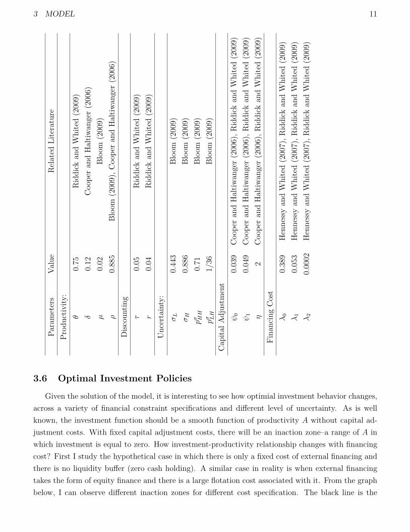
Tauchen and Hussey (1991)and Adda and Cooper (2003) to form a markov-chain estimate of theAR(1) process with time-varying uncertainty. This paper primarily uses the quadrature constructedby Tauchen (1986) extended to include the time-varying uncertainty. In Appendix A, a quadraticbased on Adda and Cooper (2003) with time-varying uncertainty is also constructed. The modelparameterization is from previous literature. They are listed in the following table:

8Because there are 6 variables (4 states and 2 choices), I make uncertainty binary states. In this case a matrix iscreated with 50× 50× 50× 50× 50× 2 entries for each iteration.

3 MODEL 11

Parameters

Value

Related

Literature

Prod

uctiv

ity:

θ0.75

Riddick

andW

hited(2009)

δ0.12

Coo

peran

dHaltiw

anger(2006)

µ0.02

Bloo

m(2009)

ρ0.885

Bloo

m(2009),C

oope

ran

dHaltiw

anger(2006)

Disc

ounting

τ0.05

Riddick

andW

hited(2009)

r0.04

Riddick

andW

hited(2009)

Uncertainty:

σL

0.443

Bloo

m(2009)

σH

0.886

Bloo

m(2009)

pσ HH

0.71

Bloo

m(2009)

pσ LH

1/36

Bloo

m(2009)

Cap

italA

djustm

ent

ψ0

0.039

Coo

peran

dHaltiw

anger(2006),R

iddick

andW

hited(2009)

ψ1

0.049

Coo

peran

dHaltiw

anger(2006),R

iddick

andW

hited(2009)

η2

Coo

peran

dHaltiw

anger(2006),R

iddick

andW

hited(2009)

Fina

ncingCost

λ0

0.389

Hennessyan

dW

hited(2007),R

iddick

andW

hited(2009)

λ1

0.053

Hennessyan

dW

hited(2007),R

iddick

andW

hited(2009)

λ2

0.0002

Hennessyan

dW

hited(2007),R

iddick

andW

hited(2009)

3.6 Optimal Investment Policies

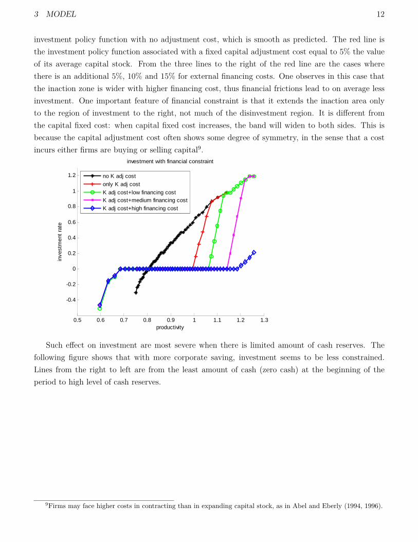
Given the solution of the model, it is interesting to see how optimial investment behavior changes,across a variety of financial constraint specifications and different level of uncertainty. As is wellknown, the investment function should be a smooth function of productivity A without capital ad-justment costs. With fixed capital adjustment costs, there will be an inaction zone–a range of A inwhich investment is equal to zero. How investment-productivity relationship changes with financingcost? First I study the hypothetical case in which there is only a fixed cost of external financing andthere is no liquidity buffer (zero cash holding). A similar case in reality is when external financingtakes the form of equity finance and there is a large flotation cost associated with it. From the graphbelow, I can observe different inaction zones for different cost specification. The black line is the

3 MODEL 12

investment policy function with no adjustment cost, which is smooth as predicted. The red line isthe investment policy function associated with a fixed capital adjustment cost equal to 5% the valueof its average capital stock. From the three lines to the right of the red line are the cases wherethere is an additional 5%, 10% and 15% for external financing costs. One observes in this case thatthe inaction zone is wider with higher financing cost, thus financial frictions lead to on average lessinvestment. One important feature of financial constraint is that it extends the inaction area onlyto the region of investment to the right, not much of the disinvestment region. It is different fromthe capital fixed cost: when capital fixed cost increases, the band will widen to both sides. This isbecause the capital adjustment cost often shows some degree of symmetry, in the sense that a costincurs either firms are buying or selling capital9.

0.5 0.6 0.7 0.8 0.9 1 1.1 1.2 1.3

-0.4

-0.2

0

0.2

0.4

0.6

0.8

1

1.2

investment with financial constraint

productivity

inve

stm

ent

rate

no K adj cost

only K adj cost

K adj cost+low financing costK adj cost+medium financing cost

K adj cost+high financing cost

Such effect on investment are most severe when there is limited amount of cash reserves. Thefollowing figure shows that with more corporate saving, investment seems to be less constrained.Lines from the right to left are from the least amount of cash (zero cash) at the beginning of theperiod to high level of cash reserves.

9Firms may face higher costs in contracting than in expanding capital stock, as in Abel and Eberly (1994, 1996).

3 MODEL 13

0.5 0.6 0.7 0.8 0.9 1 1.1 1.2 1.3-0.6

-0.4

-0.2

0

0.2

0.4

0.6

0.8

1investment with cash holding

productivity

inve

stm

ent

rate

no cash

low cash

financing cost 5%financing cost 10%

financing cost 15%

However, the pattern changes when cash holding is introduced. A liquidity buffer sufficientlylarge provides leeway in capital spending. With the fixed financing cost combined, firms will find itcostless to spend up to their cash reserves, but any amount of investment greater than that will resultin financing costs. Therefore, if the cash reserves are sufficiently large, there will be an additonalrange of productivity for which a flat investment policy function is observed and this region mightnot coincide with the investment inaction zone.

0.6 0.7 0.8 0.9 1 1.1 1.2 1.30

0.5

1

1.5

2

2.5investment with financial constraint

productivity

inve

stm

ent

rate

no K adj cost

only K adj cost



The analysis above indicates that fixed financing cost further constrain investment in two ways:First it induces more inaction on capital expansion but no symmetric effect on capital contraction.Second it creates more inertia in capital spending, which further exacerbate underinvestment. More-over, corporate saving works as means to alleviate this problem–with more liquidity I see shrinkingof the inaction and inertia regions.

3 MODEL 14

3.6.1 Uncertainty

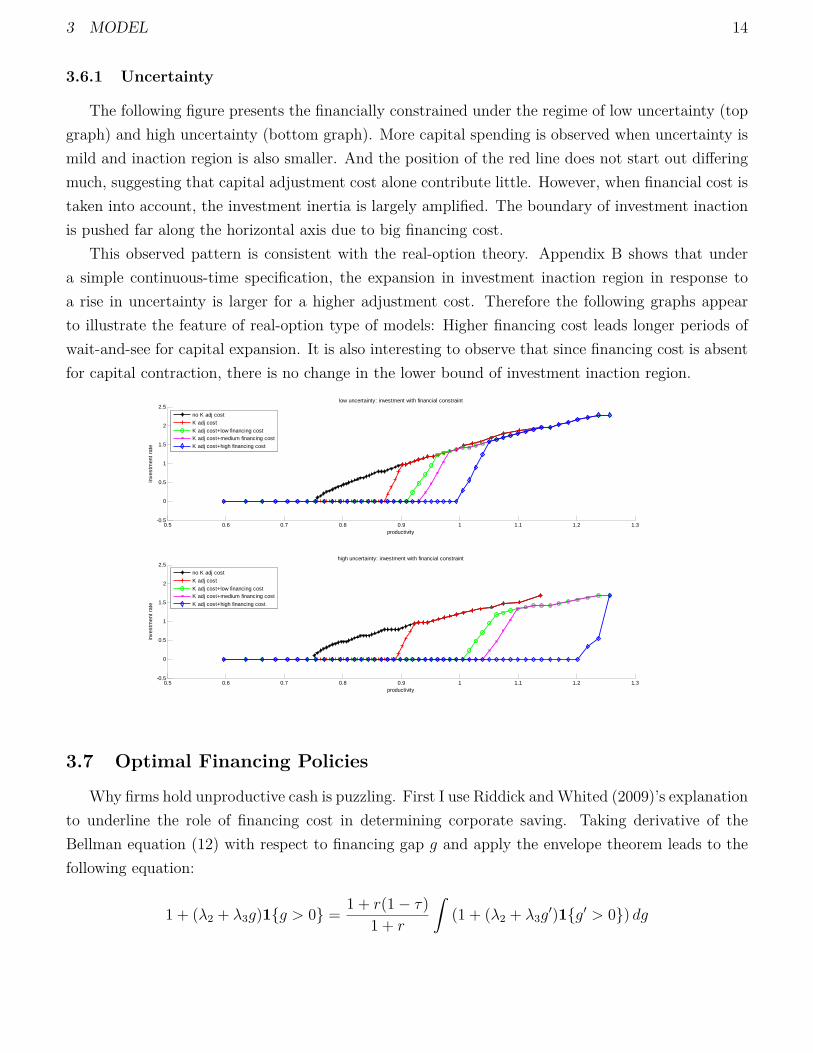
The following figure presents the financially constrained under the regime of low uncertainty (topgraph) and high uncertainty (bottom graph). More capital spending is observed when uncertainty ismild and inaction region is also smaller. And the position of the red line does not start out differingmuch, suggesting that capital adjustment cost alone contribute little. However, when financial cost istaken into account, the investment inertia is largely amplified. The boundary of investment inactionis pushed far along the horizontal axis due to big financing cost.

This observed pattern is consistent with the real-option theory. Appendix B shows that undera simple continuous-time specification, the expansion in investment inaction region in response toa rise in uncertainty is larger for a higher adjustment cost. Therefore the following graphs appearto illustrate the feature of real-option type of models: Higher financing cost leads longer periods ofwait-and-see for capital expansion. It is also interesting to observe that since financing cost is absentfor capital contraction, there is no change in the lower bound of investment inaction region.

0.5 0.6 0.7 0.8 0.9 1 1.1 1.2 1.3-0.5

0

0.5

1

1.5

2

2.5low uncertainty: investment with financial constraint

productivity

inve

stm

ent

rate

no K adj cost

K adj cost



0.5 0.6 0.7 0.8 0.9 1 1.1 1.2 1.3-0.5

0

0.5

1

1.5

2

2.5high uncertainty: investment with financial constraint

productivity

inve

stm

ent

rate

no K adj cost

K adj cost



3.7 Optimal Financing Policies

Why firms hold unproductive cash is puzzling. First I use Riddick andWhited (2009)’s explanationto underline the role of financing cost in determining corporate saving. Taking derivative of theBellman equation (12) with respect to financing gap g and apply the envelope theorem leads to thefollowing equation:

1 + (λ2 + λ3g)1{g > 0} = 1 + r(1− τ)1 + r

ˆ(1 + (λ2 + λ3g

′)1{g′ > 0}) dg

4 EMPIRICAL PREDICTIONS 15

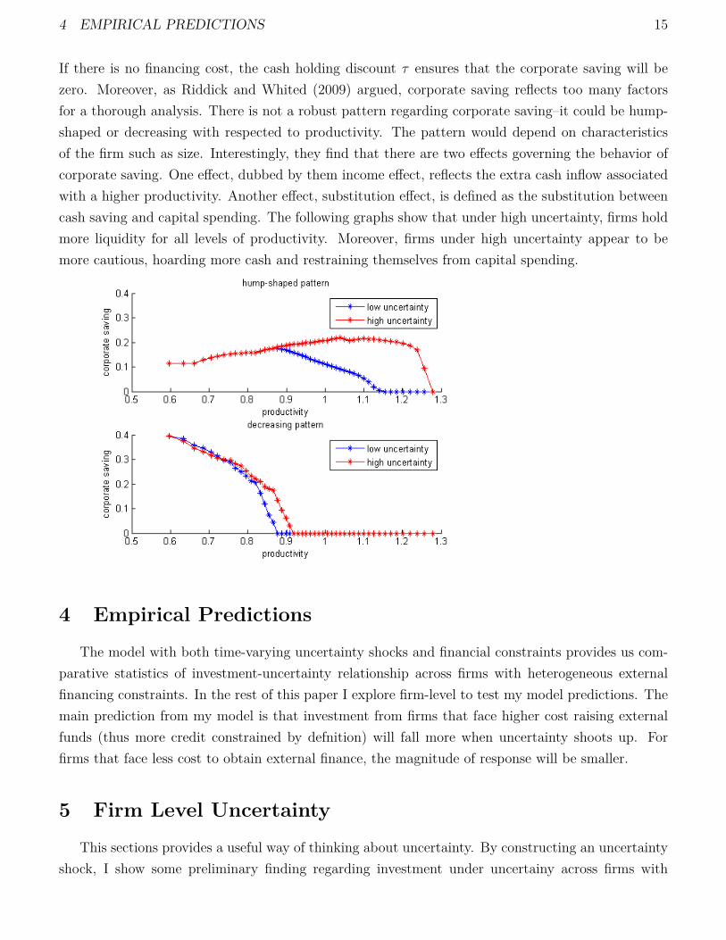
If there is no financing cost, the cash holding discount τ ensures that the corporate saving will bezero. Moreover, as Riddick and Whited (2009) argued, corporate saving reflects too many factorsfor a thorough analysis. There is not a robust pattern regarding corporate saving–it could be hump-shaped or decreasing with respected to productivity. The pattern would depend on characteristicsof the firm such as size. Interestingly, they find that there are two effects governing the behavior ofcorporate saving. One effect, dubbed by them income effect, reflects the extra cash inflow associatedwith a higher productivity. Another effect, substitution effect, is defined as the substitution betweencash saving and capital spending. The following graphs show that under high uncertainty, firms holdmore liquidity for all levels of productivity. Moreover, firms under high uncertainty appear to bemore cautious, hoarding more cash and restraining themselves from capital spending.

4 Empirical Predictions

The model with both time-varying uncertainty shocks and financial constraints provides us com-parative statistics of investment-uncertainty relationship across firms with heterogeneous externalfinancing constraints. In the rest of this paper I explore firm-level to test my model predictions. Themain prediction from my model is that investment from firms that face higher cost raising externalfunds (thus more credit constrained by defnition) will fall more when uncertainty shoots up. Forfirms that face less cost to obtain external finance, the magnitude of response will be smaller.

5 Firm Level Uncertainty

This sections provides a useful way of thinking about uncertainty. By constructing an uncertaintyshock, I show some preliminary finding regarding investment under uncertainy across firms with

5 FIRM LEVEL UNCERTAINTY 16

heterogeneous financial constraints before going into a full-fledged panel estimation.

5.1 Measuring Firm-Level Uncertainty

Uncertainty comes in many forms. When firms make investment decisions, the future productivity,price, wage, demand, regulations, exchange rates and taxes are all uncertain. An ideal measure ofuncertainty would includes all of those uncertainty. These data are hard to construct and I lackdisaggregate measures of these uncertainty. The uncertainty I try to capture is aimed to reflectfuture expectations. Following Leahy and Whited (1996), Bond and Cummins (2004)and Bloom etal. (2007), I argue that the volatility of firm’s securities summarizes the firm’s uncertainty. Theadvantage is that since this is a stock market based measure, it reflects all the information investorscare about and it is a forward-looking measure. Since the uncertainty I are measuring is relatedto the information in the future, it is important to exlude the ex-post information. The implied-volatility is another natural measure of that but the limitation of the data availability preventedus from constructing uncertainty based on that. Instead I have sufficient disaggregate and highfreqency date from CRSP stock price data and under the assumption that a company’s stock pricereflect information regarding all the uncertainty listed above, I can construct a general measure ofuncertainty. However, my measure of uncertainty is not exactly the same as Leahy and Whited (1996)and Bond and Cummins (2004), because I are concerned about their normalization of the uncertaintyby the debt-to-equity ratio (See Appendix C for details).

The downside of this measure of uncertainty is that such measure tends to be noisy. It maydepart from the fundamental economic uncertainty due to a variety of observations in the market,such as bubbles, noise trading etc. To address this concern, I take the difference between daily returnand the S&P 500 market return to control for the aggregate market bubble, panic and noise. I alsoconstruct a measure of uncertainty based on monthly stock returns. I argue that such a measuremight be better if high-frequency data are more likely to be impacted by market irrational behaviors.Bond and Cummins (2004) study three uncertainty measures: the measure I use–volatility from dailystock returns, the disagreement among securities analysts on future profitability, and the variance offorecast errors. They show that all three measures are positively correlated and to some extent theyall capture the underlying movements in uncertainty. From their results, I argue that this measureof uncertainty, despite the fact that it is noisy, reflect the economic uncertainty I deem important.

5.2 Uncertainty Shocks

Before I do a rigorous econometric analysis, I would like to explore graphically the propertyof uncertainty and its relationship with firm investment. Leahy and Whited (1996) and Bloom etal. (2007) use year-around standard deviation of daily stock returns as a measure of firm-specificuncertainty. To reconcile my result with Bloom (2009), I need to construct a shock of uncertaintyat firm-level. However, the measure of a firm-level uncertainty shock requires thought. To this end I


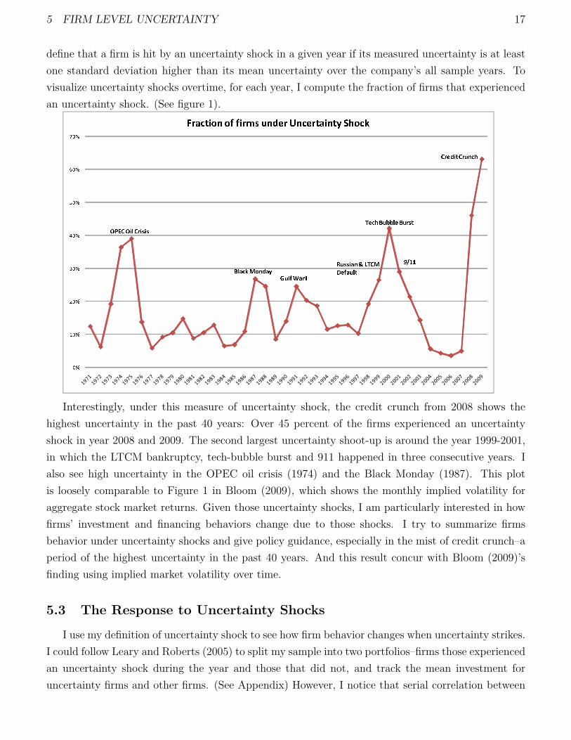
define that a firm is hit by an uncertainty shock in a given year if its measured uncertainty is at leastone standard deviation higher than its mean uncertainty over the company’s all sample years. Tovisualize uncertainty shocks overtime, for each year, I compute the fraction of firms that experiencedan uncertainty shock. (See figure 1).

�� !��"��#

Interestingly, under this measure of uncertainty shock, the credit crunch from 2008 shows thehighest uncertainty in the past 40 years: Over 45 percent of the firms experienced an uncertaintyshock in year 2008 and 2009. The second largest uncertainty shoot-up is around the year 1999-2001,in which the LTCM bankruptcy, tech-bubble burst and 911 happened in three consecutive years. Ialso see high uncertainty in the OPEC oil crisis (1974) and the Black Monday (1987). This plotis loosely comparable to Figure 1 in Bloom (2009), which shows the monthly implied volatility foraggregate stock market returns. Given those uncertainty shocks, I am particularly interested in howfirms’ investment and financing behaviors change due to those shocks. I try to summarize firmsbehavior under uncertainty shocks and give policy guidance, especially in the mist of credit crunch–aperiod of the highest uncertainty in the past 40 years. And this result concur with Bloom (2009)’sfinding using implied market volatility over time.

5.3 The Response to Uncertainty Shocks

I use my definition of uncertainty shock to see how firm behavior changes when uncertainty strikes.I could follow Leary and Roberts (2005) to split my sample into two portfolios–firms those experiencedan uncertainty shock during the year and those that did not, and track the mean investment foruncertainty firms and other firms. (See Appendix) However, I notice that serial correlation between


uncertainty shocks and its first lag is 0.15, and the rest of lags negative and close to zero. This imposesa serious problem with this methodology, making the pre- and post-uncertainty-shock investment fallas well. Therefore, I construct a simple model to account for serial correlation in uncertainty. mychoice is a reduce-form specification of autoregressive distributed lag (ADL) model and impose anAR(1) structure on uncertainty shocks:

(I

K

)it

= α(I

K

)it−1

+ βXit +k∑j=0

γjσit−j + uit

σit = φσit−1 + εit

In this construction,(IK

)itis the investment rate, Xit is the vector of control variables and σit is the

uncertainty shocks. I use firms’ cash flow and its lags, its interaction with uncertainty, average Qand year dummy for control variables. The variables I choose is based on Lamont (1997). This isthe regression studies typically use for estimation on a panel data. Three lags in the uncertainty lagspecification are chosen to show the time dynamics and ensure not many data points are dropped dueto length and consistency of the data. For simplicity, I assume the error terms from the two equations,uit and εit are uncorrelated. An impulse response and its corresponding 95% confidence band areconstructed based on the panel coefficient estimates (See Appendix). The horizontal axis indicatesthe year pre and post uncertainty shock with zero the year of impact. I see a 10% contemporaneoussharp decline in investment rate when an uncertainty shock arrives. And after 2 years it reverts backto its orginal level and overshoots after. And the changes at the year of impact and the year afterare significant in terms of the confidence band. This is consistent with Bloom (2009)’s finding onaggregate time series.


-.15

-.1

-.05

0.0

5.1

.15

inve

stm

ent r

ate

-1 0 1 2 3year

Uncertainty Impulse Response

As a first pass to study the impact of financial frictions, I decompose my sample to five subgroupsbased on size (capital). In corporate finance literature, size is found to be an important determinantfor financial frictions. For example, Fazzari et al. (1988) found systematic evidence that liquidityconstraints tend to be more binding for smaller firms. In a seminar paper on financial frictions,Petersen and Rajan (1994) observe that small and young firms are most likely to face more informationasymmetry in lending relationship and therefore credit rationed. Bernanke et al. (1999) explicitlyuse firm size (capital) as a collateral for external financing and suggested that bigger firms are ableto obtain more financing. Firm size, albeit imperfect, is a measure researchers commonly used forempirical studies of corporate financing constraints10. my results for different size quintiles show thatfor the firms in the top quintile (top 20% percentile), the drop is merely 3% and it moves back quicklyafter one year and the drop is not statistically significant. The firms in the bottom quintile (bottom20 percentile), however, has experience large and statistically significant fall in investment rate (closeto 15%) and reverts slowly back to its orginal level after three years.

10An imcomplete list is Devereux and Schiantarelli (1990) for UK firms, Athey and Laumas (1994) for indian firms,Gilchrist and Himmelberg (1995) for US data, Kadapakkam et al. (1998) for firms from six OECD countries, etc.


-.2

-.15

-.1

-.05

0.0

5.1

.15

.2

-1 0 1 2 3year

0-20%

-.2

-.15

-.1

-.05

0.0

5.1

.15

.2

-1 0 1 2 3year

20%-40%

-.2

-.15

-.1

-.05

0.0

5.1

.15

.2

-1 0 1 2 3year

40%-60%

-.2

-.15

-.1

-.05

0.0

5.1

.15

.2-1 0 1 2 3

year

60%-80%

-.2

-.15

-.1

-.05

0.0

5.1

.15

.2

-1 0 1 2 3year

80%-100%

Vertical Axis: Investment RateSize Quintiles From Left to Right: <20%, 20%-40%, 40%-60%, 60%-80%, >80%

Uncertainty Impulse Response, by Size

Whited (1992) split sample into firms with bond rating and firms without bond rating to studyliquidity constraint and firm investment. She argues that firms with bond rating have less informationasymmetry, so it is easier for them to obtain debt financing and they are in this sense less financiallyconstrained. Following her criteria, I divide my sample based on whether a firm has a bond ratingor not. In this cas I see more striking results: Firms with bond rating virtually do not fall andinsignificantly from zero for all the years after impact. whereas all the drop are from firms with nobond rating.


-.15

-.1

-.05

0.0

5.1

.15

-1 0 1 2 3year

Unrated

-.15

-.1

-.05

0.0

5.1

.15

-1 0 1 2 3year

Rated

Vertical Axis: Investment Rate

Uncertainty Impulse Response, by Bond Rating

In an influential paper, Fazzari et al. (1988) categorize firms according to dividend payouts tostudy financing constraints and corporate investment. I do the same exercises in terms of the amountof dividend paid. For firms that pays a lot of dividends, the decline in investment rate is very minimal(2%) and quickly reverts back. The fall in these two categories are insignificant from zero. Firmsthat do not pay dividend (<25%) or pay very little (25%-50%) experienced very large drop.

-.25

-.2

-.15

-.1

-.05

0.0

5.1

.15

.2

-1 0 1 2 3year

0-25%

-.25

-.2

-.15

-.1

-.05

0.0

5.1

.15

.2

-1 0 1 2 3year

25%-50%

-.25

-.2

-.15

-.1

-.05

0.0

5.1

.15

.2

-1 0 1 2 3year

50%-75%

-.25

-.2

-.15

-.1

-.05

0.0

5.1

.15

.2

-1 0 1 2 3year

75%-100%

Vertical Axis: Investment RateDividend Payout Quartiles From Left to Right: <25%, 25%-50%, 50%-75%, 75%-100%

Uncertainty Impulse Response, by Divdend Payout

6 EMPIRICAL RESULTS 22

All the results above are consistent with my predictions that investment from financially con-strained firms behaves very differently from financially unconstrained firms. Imposing a simple struc-ture on the dynamics of investment and uncertainty allows me to see the dynamics of how investmentbehaves upon an uncertainty shock and how they are different across firms with heterogeneous fi-nancial constraints. It is important for us to visualize the effect which allows for further empiricalinvestigations. The downside of such a simple specification is that it might be too restrictive for myanalysis. In the next section, I use more regressions and more proxies of financial frictions to test mypredictions.

6 Empirical Results

6.1 Data and Summary Statistics

In this section I study more of the response to uncertainty for publicly-traded companies. Thedata are from the US non-financial firms in the 2010 Standard and Poor’s Compustat industrialfiles. The firm-level data constitutes an unbalanced panel from 1971 to 2009. The Compustat datais augmented with standard deviation of daily stock return data from The Center for Research inSecurity Prices (CRSP) data.

I drop firm-year observations from my sample with missing or negative values for total asset andfirms that has observations for less than three consecutive years. I delete all firms whose primaryStandard Industrial Classification (SIC) code is between 4900 and 4999, between 6000 and 6999 orgreat than 9000, because my models of investment is inappropriate for regulated and financial firms.Firm-years that involved in significant merger and acquisitions (greater than 15% of book asset value)during the sample period are also excluded. I constructed the replacement value of capital stock usingthe perpetual inventory method described in Salinger and Summers (1983) (Appendix). I normalizefirm investment (capital expenditure), cash flow, cash holding by the replacement value of capitalstock at the end of last fiscal year. All the variables I use are winsorized 1% on both ends of thedistribution. It is important to include a measure of Tobin’s Q, which captures all future profitabilityfor a firm. According to Hayashi (1982), I use an average Q for Tobin’s Q, which is defined by themarket value divided by capital replacement value.

Summary statistics are in Table 1. Firms’ average investment rate is 0.76 and median is 0.42and it is quite right-skewed. my prediction is that rise in uncertainty leads to a fall in investment.In this case, the magnitude of the fall should be compared with the investment distribution here todetermine its significance. Similary, asset, capital stock and cash holding all have distributions thatare right-skewed.


6.2 Specification

I use three estimation strategies to identify the impact of uncertainty shock to investment: OLS,fixed effect and dynamic panel regression (Holtz-Eakin et al. (1988), Arellano and Bond (1991), Bond(2002)). For all three strategies, I add year dummies to control for time-specific effects. Dynamic panelregressions are used to partly address my endogeneity concern–it allows the regressors I used to beendogeneous. In addition, in this estimation I first-difference all the variables for GMM estimationand this removes unobserved firm-specific effects, which could be correlated with regressors andgenerate biased results. Following Arellano and Bond (1991) and Bond and Cummins (2004), I treatuncertainty as an endogenous variable and choose the second and third lags for investment, cashflow, uncertainty and their interactions as instruments. I use heteroskedasticity-consistent standarderrors and test statistics. I report the Hansen overidentification test and Arellano and Bond (1991)’stest for first order serial correlations. For comparison I find it useful to compare it to the resultsfrom OLS and fixed effect regressions. In terms of control variables, I use the cash flow and itslags, because the consensus in the literature that cash flow has strong relationship with corporateinvestment (Fazzari et al. (1988), Blanchard et al. (1994), Lamont (1997)). I also include cash flow’sinteraction with uncertainty. Here I do not include average Q for control variable because of theproblematic measurement issues with this measure as future investment opportunities. But I willinclude it later for my robustness checks.

6.3 Baseline Regressions

Table 2 (Left panel) shows the results of the regressions of investment-to-capital ratio ( ItKt−1

, alsocalled investment rate) on uncertainty (σt) and I observe that coefficients are significantly negativefor OLS, fixed effect and dynamic panel regresssions and their magnitudes are similar. However, sinceHansen’s overidentification test indicates that my instruments are rejected, the estimates under GMMin the dynamic panel regressions should be used with caution. Nonethelss, my estimates are consistentwith the theoretical predictions that uncertainty shocks lower investment. Given the magnitude ofthe coefficient and the mean of uncertainty and the regression coefficient, I infer that a one standarddeviation increase in volatility (uncertainty) leads to a drop of over 10% in investment-to-capitalratio, which loosely match the result in the impulse response of uncertainty shocks. I also observethat the interaction term for cash flow and uncertainty has a significant negative relationship withinvestment ratio. This is the evdence that higher uncertainty makes firms less responsive to cashflow. I notice that the drop of 10% in investment-to-capital ratio is in absolute term – but how isthis decrease measured in relative term? To answer this question, I also construct the change rateof investment rate. Because investment is a flow measure and it can be negative, in which case itcomplicates the measure of growth rate11 I dropped all investment that is negative at the beginning of

11When investment is negative, the investment growth measure of a negative investment at time t-1 and positiveincrement from time t-1 to time t would be yield the same sign as in the case where the investment at time t-1 ispositive the increment is negative.


the period, which is 11% of all my observations, construct the investment growth rate and winsorizeit at 1% and 99% to avoid outliers. I do the same regressions on the growth rate of investment rateand I find that a one standard deviation (33%) increase in uncertainty leads to a 35% drop in OLS,45% drop in fixed effect regressions and 43% in dynamic panel regressions for relative terms.

6.4 Regressions for Financially Constrained Firms

I use three criteria to obtain reasonable measures of financial frictions at the firm-level. Firm’sasset, bond rating, dividend payout and the Kaplan-Zingales index, albeit their imperfections, arewidely adopted to proxy for financial constraints. And I follow previous literature to use samplesplitting based upon each measure to study the behavior of firms with different access to financialconstraints. Following Bond et al. (2004) and Chen et al. (2010), each firm is marked in one subsamplein all its sample years.

Small firms are considered difficult to obtain external fund and big firms normally have easieraccess to various forms of financing, relationship banking, bond market etc.. I partition firms thatdiffer in their asset size to proxy for a spectrum of credit conditions. The median asset is calculatedfor a firm in all its sample years and use it to split my sample into 10 subsamples. Table 3 shows thesummary statistics of those subsamples. The investment rate across different groups are quite similar.It is only slightly smaller for larger firms. The standard deviation of investment rate, however, ishigher for smaller firms. For uncertainty, I observe an decreasing pattern: smaller firms seem tosubject to larger uncertainty. It is consistent with my understanding that smaller firms have morevolatile growth prospects than larger firms. Cash flow is on average monotonically larger for biggerfirms and its standard deviation higher for smaller firms. I also see that the asset holding is veryright skewed.

From the OLS regressions (Table 4A), I observe for subgroups from the first eight deciles, therelationship between investment rate and uncertainty shows a negative sign and statistically significantfrom zero. In contrast, largest firms in the top quintile (top two deciles) of the sample do not respondsignificantly to uncertainty shocks. Larger firms tend to have weaker response to uncertainty shocks,although the pattern is not monotonic. The R squared is smaller for smaller firms (less than tenpercent for the first three decile), and grow close to 40 percent for the largest decile. The interactionterm of cash flow and uncertainty does not have a significant impact on investment rate. In Table 4BI use fixed effect model to purge the time-invariant effect for each firm. The results are quite similarto those from OLS. Larger firms appear to have weaker relationship with the level of uncertainty butthe effect is not montonic. The R squared are very similar too. Table 4C shows us the results fromdynamic panel regressions. The pattern is similar to what I see in fixed effect regressions. However,there is no significant uncertainty-investment relationship for the smallest size decile. The coefficientfrom this specification is larger than the other regressions. However, the Hansen J-test tells us thatthe results is only instrument-proof for only top two quintiles These finding are largely consistentwith my prediction that firms that are credit constrained tend to fall more due to uncertainty while


unconstrained firms are less responsive.Borrowers use bond ratings to assess a firms’ credit quality. According to Whited (1992), firms

that use the corporate bond market are subject to more investor scrunity so that they are moretransparent and suffer less information asymmetries. By the same argument, firms without a bondrating are typically hard to raise funds on the debt market, therefore they tend to have more bindingfinancial constraint. Table 5 shows us the summary statistics: First, there are lot more firms withoutbond rating than firms with bond ratings–the ratio is 12 to 1, meaning there is only one firms thathave bond rating out of thirteen firms. Firms with bond ratings are more than ten times larger inasset. Investment rate is slightly bigger for firms without bond rating and the standard deviationfor unrated firms is twice the number of rated firms. Uncertainty on firms without rating is twiceas large as the firms with bond rating both in terms of mean and standard deviation. Average cashflow is much smaller (negative) for unrated firms and the difference in mean is almost 100%. Thestandard deviation of cash flow on firms without rating is fmy folds the firms with bond rating.

From the regressions results of Table 6, I observe that the coefficients on uncertainty are insignif-icant for firms without bond rating. Uncertainty of the bond rated firms, however, are negative andsignificant. The results are robust across OLS ,fixed effect estimations and dynamic panel estima-tions. R squares of firms with bond rating over 25 percent higher than firms without bond rating.The magnitude of the drop in investment rate with respect to uncertainty is quite similar to the creditconstrained firms defined in terms of sizes: A one standard deviation increase in standard deviationwould result in over ten percent lower investment rate. Given the assumption that bond rating is avalid measure of financial constraints, the results here is also consistent with my predictions.

Dividend payout has been an important measure used in corporate finance researches to identifyfinancial constraints. Fazzari et al. (1988) argues that the retention practice provides us a usefulmeasure, because cost disadvantage of external finance would have a larger effect on firms that retainmost of their earnings while firms that distribute a lot of their earnings would be less effected bythe cost of external finance. Other work in corporate finance also shows that firms that are moreconstrained financially tend to pay out less dividend (Bolton et al. (2009), Faulkender and Wang(2006)). However, I am well aware of the debate on whether dividend payout ratio provides a goodmeasure of financial constraint (Kaplan and Zingales (1997), Fazzari et al. (2000), Kaplan and Zingales(2000)). This paper does not provide additional insight on whether it is a good measure of financialconstraints. I make the assumption that dividend payout ratio reveals certain level of firms’ financialcondition and use their methodology to proxy for financian constraints. The sample is splitted intofour subsamples using the amount of dividend distribution. I also try the dividend-capital ratio Table7 is the summary statistics across these subgroups. The first subgroup virtually pay no dividend andthe second subgroup pay very little. The investment rate is not very different but the standarddeviation across subgroups is large. Uncertainty is higher for firms that pay less dividend but thestandard deviation is similar. Firms that pay less dividend have more negative cash flow and largerstandard deviations than firms that pay more dividend.


Table 8A, 8B and 8C show the regression output that the top quartile dividend distributors donot respond to uncertainty significantly in both OLS, fixed effect and dynamic panel specifications.Under OLS and fixed effect estimations, uncertainty coefficients on investment rate for subgroups inthe first three quartiles are negative and very significant. The R squares are lower for firms that payno or less dividend and it is over twenty percent for firms in the top quartile. However, the significanceon uncertainty is not there for non-dividend-payers in Table 8A. Again, the it is hard to be convincedbecause the Hansen test suggests instruments are not valid. All the above results provide anotherevidence that more financially constrained firms respond more negatively to an uncertainty shock.

Kaplan-Zingales Index (Kaplan and Zingales (1997), Kaplan and Zingales (2000)) is anothermeasure of financial friction, constructed based on a variety of variables. From a survey responseof financial conditions, they estimated a relationship of a given set of variables to firms’ financialstate. This provides an score of financial constrainedness for every firm based upon various variablesof interest as follows:

−1.001909 CFitAit−1

+ 3.139193LEVit − 39.3678DIVitAit−1

− 1.314759 CitAti−1

+ 0.2826389Qit

where CFitAit−1

is cash flow over lagged assets; DIVitAit−1

is cash dividends over assets; CitAti−1

is cash balancesover assets; LEVit is leverage; and Qit is the market value of equity (price times shares outstandingfrom CRSP) plus assets minus the book value of equity all over assets. And following Baker etal. (2003), I winsorize every variable at 1% and 99%. The Kaplan-Zingales index has been usedextensively as a measure of financial constraints (Lamont et al. (2001), Hennessy et al. (2007), Bakeret al. (2003) for example). However, Almeida et al. (2004), Whited and Wu (2006) and Hadlock andPierce (2010) question the validity of Kaplan-Zingales index as a measure of financial constrainedness.

Summary statistics is in Table 9. Investment rate appear to be an upper trend across deciles.The less financially constrained from the left, measure by KZ index, have lower average investmentrate and lower volatility of investment rate. The mean and standard deviation seem to be quiteclose. Cash flow is lower for financially constrained firms in the upper deciles and its correspondingstandard deviations higher. Financially unconstrained firms are larger in terms of size, especially forthe bottom decile (0-10%).

From Table 10A, I observe that there is only one coefficient on uncertainty that is not significant–That is the one for the most financially unconstrained firms measure by KZ index in the first decile.And coefficients on the second and third deciles have significance at 5% while the rest are significantat 1%. Although the result is not very impressive, it is suggestive of my story that investment ratefrom unconstrained firms, compared to investment rate from its constrained counterparts, are lessrepsonsive to an uncertainty shock. Table 10B presents a result that is in general consistent with mystory, although the coefficient on the second decile is quite significant and its magnitude surpassesthat of the third decile. Table 10C presents us with more interesting results. I find that top fortypercent of the firms’ investment behaviors are significantly affected by uncertainty. The magnitudesof investment adjustment are different across firms.

7 POLICY IMPLICATIONS 27

However, Leahy and Whited (1996) find insignificant investment response in a regression of in-vestment rates on the measure of uncertainty same as ours. From my results, I understand thatunconstrained firms will show a coefficient that is insignificant and constrained firms show significantcoefficient. Therefore, based on this reasoning, the overall regression might show a significant orinsignificant coeffcient depending on what kind of firms dominate.

6.5 Robustness

Because I are studying the second-moment effect, it is important to control for the first-ordereffect–the average profitability . Because I measure the second-moment shock using the stock returnvolatility, I try both the mean stock return and average q to control for the first-order effect. Leahyand Whited (1996) see their uncertainty effect disappear after they control for average Q and thusargue that uncertainty affects investment only through Q. But here I see that Q does not affect mymain results.

Firm size is the main determinant of financial frictions. But firm size is important affecting otherthings other than financial frictions, such as productivity and industry-level effects. my finding relatedto financial frictions might be driven solely by firm size. I include capital stock in every regression Irun, although it appears to be significant in most of regressions, my main finding remains robust.

7 Policy Implications

In the crisis starting the fourth quarter of 2007, I have been experiencing a dramatic increasein uncertainty, in magnitudes I find similar in the era of the Great Depression. In such a period ofhigh uncertainty, the usual policy instruments might not be as effective as it is in normal times. Inparticular,Bloom (2009) argues that high uncertainty induces more wait-and-see in investment andhiring for firm and stimulus policies in high-uncertainty espisodes may not be effective. From mystudy, I look closer into the uncertainty-investment relationship in the historical firm-level data. myresults are partially consistent with his argument. Interestingly, I find that the uncertainty-investmentrelationship is heterogeneous among firms with different access to credit market. For firms that haveeasier access to credit market, the uncertainty-investment relationship is much lower.

Therefore, there are two important policy implications. The first implication is related to hetero-geneity across firms: my study suggests that a stimulus policy might affect firms differently. Firmswith without much financing opportunities will be more affected in high-uncertainty episodes andthey may also be those firms that are not very responsive to any stimulus (either from demand sidestimulus such as ones stimulating consumer spending or firm stimulus such as tax benefits). I alsoshow that small firms are the ones more affected and a customized policy for those firms distinguish-ing those firms from those with good credit conditions might be important. To induce quick policyresponse from those firms facing high cost accessing credit markets, policy makers might want toimprove their credit standings and provide them with more access to liquidity.

8 CONCLUSION 28

The second implication is related to heterogeneity across time. Firms face different credit condi-tions in different times. Borrowing in 2008 in very difficult, however, just two years earlier in 2006,firms enjoy very good credit conditions. Although time-varying credit conditions is not a feature inmy model, nonetheless I try to make conjectures based on my results. Because I show that financingcondition may be an important factor that affects the uncertainty-investment relationship, I expectthat a credit crunch will amplify the impact of uncertainty on firm investment and hiring. Firms willbe even less willing to respond to stimulus. In this situation I suggest that either improving firms’credit condition or lowering the level of uncertainty could be useful to make firm spend on capital orhiring.

8 Conclusion

This paper study the relationship among uncertainty, financial constraint and investment. Themain finding is that investment from firms with different financial frictions responds differently touncertainty. I show that this finding is consistent with a model which incorporates non-convexadjustment cost, time-varying uncertainty and financial frictions.

my paper has important contributions. Theorectially this is among the first models to study theinteraction of the relationship of all three variables. I contribute to the macroeconomic productionmodels by incorporating both firm’s external financing and saving and time-varying uncertainty. mycontribution to the corporate finace literature is modeling the second-order volatility effect in a modelwith investment and financing decisions. On the empirical side, this is the first paper to study theuncertainty-investment relationship across different firm groups. I contribute to a long literaturestudying the relationship of firm investment and their financing conditions(Fazzari et al. (1988),Kaplan and Zingales (1997) etc). I find another way that financing condition affects firm investment.my empirical finding also adds to the list of studies for uncertainty-investment relationship (Leahyand Whited (1996), Baum et al. (2008), Bloom (2009)) .

I also derive interesting policy implications from my study. my model suggests that an effectivestimulus policy for firms would take into account the differentials on firms’ credit condtions. Smallerand more credit constrained firms are less responsive to policy in an episode of high uncertainty.Therefore policies targeted to effectivly stimulate those firms may also address their liquidity concerns.

A NUMERICAL SOLUTION 29

APPENDIX

A Numerical Solution

A.1 Algorithm

I use value function iteration (Judd (1998), Adda and Cooper (2003)) on the state variables(K,P,A, σ) to achieve convergence by the following algorithm:

Set grid points for each of the fmy states (K,P,A, σ). In this study I use 50×50×50×2 = 250, 000points for most of my results. I try finer grids up to 100× 100× 100× 2 = 2, 000, 000 points for somespecifications. The results are similar throughout. Grids of A and σare defined from a quadrature Iconstructed in the next section. And I also use a variant of quadrature from Tauchen (1986) that takeinto account the changing volatility and use a set of grids that are cluster more around the inactionregion, an effort to capture the change in inaction zone more accurately. The quality of quadratureis important for my study because the time-varying uncertainty largely influence expectations. Toensure thatK stay on the grid all the time and especially the case for inaction where investment isnull and the next period’s K becomes (1− δ)K, I specify grids for K as

[(1− δ)jK̄, ..., (1− δ)K̄, K̄

].

Because I define everything on the grids and their movement are also restricted to the specified grids,I do not do interpolation. And I think that this is an advantage and give us more robust results. Forthe productivity shock, because it is the logarithm of A has an AR(1) structure, I have to accountfor the Jensen correction term when taking exponential of it. I substract σ2/2 from the drift term ofthe AR(1) process.12 I define value function on the grid and iterate value function using the Bellmanequation. I start with an initial value for the value function that has the same value for every state.It takes on average 3 hours to solve the dynamic programming program, although the running timevaries with parameters.

A.2 Construction of Quadrature

In standard models with firm investment, firms make investment choices based upon their forecastof future profitability A. Because my model incorporates time-varying uncertainty, the expectationof the uncertainty change is also a deterministic factor for firms’ investment behavior. Therefore,I need to make sure that the numerical method captures the expectation well. I construct a newquadrature with time-varying volatilities based on Adda and Cooper (2003). Denote the logarithm

12In the appendix of Bloom (2009), he also address this problem by “...uncertaity effect on the drift rate is secondorder compared to the real-options effect, so the simulations are virtually unchanged if this correction is omitted”.


of technology shock A as x and x follows an AR(1) process with switching standard deviations:

x′ = µ+ ρx+ v, v ∼ N(0, σ2)

σ ∈ {σL, σH} , where Pr(σ′ = σj|σ = σk) = pk,j

µ ∈ {µL, µH} , with same transition probabilities

The reason I change µ when σ changes is because I need to account for the Jensen’s correctionterm in the mean if I want to control for the same level of change in A. The trick is that I need todefine a set of grids and transition probabilities that works for both σL and σH . First define

σ =(σLxσ

Hx

) 12

where σLx = σL√1− ρ2 and σHx = σH√

1− ρ2

µ = µLx + µHx2

where µLx = µL1− ρ and µHx = µH

1− ρ

Given the normality assumption, I define the cutoff points {xi}N+1i=1 as follows:

Φ(xi+1 − µ

σ

)− Φ

(xi − µσ

)= 1N, i = 1, ..., N

where Φ(·) is the normal cdf and solve it recursively,

xi = σΦ−1(i− 1N

)+ µ, i = 1, ..., N

=(σLxσ

Hx

) 12 Φ−1

(i− 1N

)+ µLx + µHx

2 , i = 1, ..., N

Then an important formula, which I am going to use extensively later, becomes the following:

Φ(xi+1 − µLx

σLx

)− Φ

(xi − µLxσLx

)= Φ

(σHxσLx

) 12

Φ−1(i

N

)+ µHx − µLx

2σLx

− Φ

(σHxσLx

) 12

Φ−1(i− 1N

)+ µHx − µLx

2σLx

Φ(xi+1 − µHx

σHx

)− Φ

(xi − µHxσHx

)= Φ

( σLxσHx

) 12

Φ−1(i

N

)− µHx − µLx

2σHx

− Φ

( σLxσHx

) 12

Φ−1(i− 1N

)− µHx − µLx

2σHx


Now for each interval, I define a value associated with it, zi:

zi = E(xt|xt ∈

[xi, xi+1

])= pLHpLH + pHL

σHxφ(xi−µHxσHx

)− φ

(xi+1−µHx

σHx

)Φ(xi+1−µHx

σHx

)− Φ

(xi−µHxσHx

) + µHx

+ pHLpLH + pHL

σLxφ(xi−µLxσLx

)− φ

(xi+1−µLx

σLx

)Φ(xi+1−µLx

σLx

)− Φ

(xi−µLxσLx

) + µLx

= pLHpLH + pHL

σHxφ(xi−µHxσHx

)− φ

(xi+1−µHx

σHx

)Φ((

σHxσLx

) 12 Φ−1

(iN

)+ µHx −µLx

2σLx

)− Φ

((σHxσLx

) 12 Φ−1

(i−1N

)+ µHx −µLx

2σLx

) + µHx

+ pHLpLH + pHL

σLxφ(xi−µLxσLx

)− φ

(xi+1−µLx

σLx

)Φ((

σLxσHx

) 12 Φ−1

(iN

)− µHx −µLx

2σHx

)− Φ

((σLxσHx

) 12 Φ−1

(i−1N

)− µHx −µLx

2σHx

) + µLx

Notice that for the third equation I replace expression that has Ai grids and normal in the

denominators with an expression that does not have Ai grids in it. This greatly improves accuracy.And lastly I calculate the transition probabilities. Now because I have two uncertainty states, thetransition probabilities from grid i to grid j are based on σ:

πi,j (σH) = Prob(xt ∈

[xj, xj+1

]|xt−1 ∈

[xi, xi+1

], σH

)

=´ xi+1

xie− (ε−µHx )2

2σHx{

Φ(xj+1−µH−ρε

σH

)− Φ

(xj−µH−ρε

σH

)}dε√

2πσH2x ·

{Φ(xi+1−µHx

σHx

)− Φ

(xi−µHxσHx

)}

=´ xi+1

xie− (ε−µHx )2

2σHx{

Φ(xj+1−µH−ρε

σH

)− Φ

(xj−µH−ρε

σH

)}dε√

2πσH2x ·

{Φ((

σHxσLx

) 12 Φ−1

(iN

)+ µHx −µLx

2σLx

)− Φ

((σHxσLx

) 12 Φ−1

(i−1N

)+ µHx −µLx

2σLx

)}

and

πi,j (σL) = Prob(At ∈

[Aj, Aj+1

]|At−1 ∈

[Ai, Ai+1

], σL

)

=´ xi+1

xie− (ε−µLx )2

2σLx{

Φ(xj+1−µL−ρε

σL

)− Φ

(xj−µL−ρε

σL

)}dε√

2πσL2x ·

{Φ(xi+1−µLx

σLx

)− Φ

(xi−µLxσLx

)}

=´ xi+1

xie− (ε−µLx )2

2σLx{

Φ(xj+1−µL−ρε

σL

)− Φ

(xj−µL−ρε

σL

)}dε√

2πσL2x ·

{Φ((

σLxσHx

) 12 Φ−1

(iN

)− µHx −µLx

2σHx

)− Φ

((σLxσHx

) 12 Φ−1

(i−1N

)− µHx −µLx

2σHx

)}

B INVESTMENT CRITICAL VALUE, UNCERTAINTY AND ADJUSTMENT COST 32

Thus the complete transition probabilities are

πij,LH = pLH · πi,j (σH) , πij,LL = pLL · πi,j (σL)

πij,HL = pHL · πi,j (σL) , πij,HH = pHH · πi,j (σH)

The uncertainty state here is binary. But my methodology can be extended to uncerainty statewith multiple grids.

B Investment Critical Value, Uncertainty and AdjustmentCost

This section studies the question how adjustment cost affects the relationship between investmentcritical value and uncertainty, under a simple continous-time framework. I show that in a simplereal-option framework, firms with higher adjustment cost will have larger investment inaction regionin response to high uncertainty shocks. The derivation closely follows Dixit and Pindyck (1994)Chapter 5. I consider the following problem: Firms decide when to invest with a fixed cost C in aproject of value V , which follows a geometric Brownian motion:

dV = µV dt+ σV dW (16)

Denote the present value of the project as F (V ):

F (V ) = maxE{e−ρT (VT − C)

}(17)

T is the (unkown) time the firm decides to invest and ρis the discount rate. Because there is nocash from the project until it is invested, the Bellman equation becomes

ρFdt = E(dF ) (18)

Appying Ito’s Lemma, I have

12σ

2V 2F ′′(V ) + µV F ′(V )− ρF = 0 (19)

subject to the following boundary conditions

F (0) = 0 (20)

F (V ∗) = V ∗ − C (21)

F ′(V ∗) = 1 (22)

C VARIABLE CONSTRUCTION 33

where V ∗denotes the critical value of investment, or equivalently the upper-bound for investmentinaction. And I use C to denote the cost associated with investment in this project. Firm investmentwhen the project value V exceeds V ∗. To formalize the argument V ∗satisfies V ∗ − F (V ∗) = C.

I guess the solution takes the simple form:

F (V ) = AV β (23)

By using all above equations, I have

V ∗ = β

β − 1C (24)

where β is the positive root to the quadratic equation below:

12σ

2β(β − 1) + µβ − ρ = 0 (25)

So I have a relationship betweent the investment critical value, V ∗, level of uncertainty σ2 and thenon-convex cost associated with investment C. In this paper I am interested in how the investment-critical-value-uncertainty relationship changes as I vary the capital adjustment cost C. This is asecond derivative of V ∗ with respect to both σ2 and C: ∂2V ∗

∂σ∂C. It is obvious from the formula for V ∗

that ∂V ∗

∂C= β

1−β . And if I define the quadratic equation of β as Q, then a total differentiation gives us

∂Q

∂β· ∂β∂σ

+ ∂Q

∂σ= 0 (26)

Because ∂Q∂β

and ∂Q∂σ

are both greater than zero, I have

∂β

∂σ< 0 (27)

Therefore∂2V ∗

∂σ∂C= ∂

[β

β − 1

]/∂σ = − ∂β/∂σ

(β − 1)2 > 0 (28)

This means that in this simple real-option model, the expansion of inaction region in response tohigh uncertainty, captured by ∂V ∗

∂σ, will be larger for firms with higher capital adjustment cost C.

C Variable Construction

1. Uncertainty: For each firm-year, I calculate the standard deviation of stock returns over thatfiscal year of a firm and match the financial statement information with the standard deviationof daily stock return data. For any uncertainty observation that is great than five, I trim it tofive. This construction of uncertainty is used by Bloom et al. (2007). However, unlike Leahyand Whited (1996) and Bond and Cummins (2004), I did not scale it by the debt-to-equity

D ADL IMPULSE RESPONSE 34

ratio, because I think this normalization is rather arbitrary. I do not want to complicate themeasure by adding company’s leverage, because I suspect that investment is affected by leverageratio. To illustrate my point I provide some statistics to justify this concern. The measure theyuse is σ ·

√equitydebt

. Calculations show that σ has a mean 0.038 and standard deviation 0.022while the mean and standard deviation for

√equitydebt

is more than 100× larger in comparison:5.42 and 15.76. I argue that if it is normalized, the variation of uncertainty is partly driven bythe debt-to-equity, which makes us question the validity of this uncertainty measure. Since theaverage leverage ratio is about ten percentage, my measure of uncertainty is only one tenth ofthe value in Leahy and Whited (1996)13 and Bond and Cummins (2004). Nevertheless, Bondand Cummins (2004) show results that are similar for the magnitude of investment change inresponse to a one standard deviation increase in uncertainty.

2. Replacement value of capital: Constructing an estimate of the firm’s replacement value capitalstock is necessary to correct for the bias introduced by historical cost accounting. The techniquethat I use to construct this estimate is a modification of the method used in Salinger andSummers. Several assumptions are required to construct the series and are discussed in moredetail in the Salinger and Summers paper. First, the equipment’s fixed capital has a commonuseful life (L). Second, because COMPUSTAT does not report the method that firms use todepreciate their capital stock in any detail, all firms are assumed to use straight line methodsfor book depreciation. Third, actual depreciation is exponential with rate 2/L, equivalent todouble-declining digits depreciation. Fourth, all investments are made at the beginning of theyear, and all depreciation is taken at the end of the year. Last, the value of reported grossproperty, plant and equipment in the initial year that the firm appears in the sample is equal toits replacement value, thus functioning as a seed value for the Salinger and Summers algorithm.The formula Lt = (Kt−1 + It)/DEPt provides an estimate of the useful lifetime of fixed capital.K represents the book value of gross property, plant and equipment, I is capital expenditures,and DEP is book depreciation. Instead of allowing the estimated useful life to fluctuate fromyear to year, I use each the average of each firms L. In addition, if reported depreciation is smallin any given year, L becomes implausibly large. I place an upper bound of forty years and alower bound of three years on L. The Salinger-Summers algorithm uses a method similar toperpetual inventory methods to create the replacement cost estimate of K. The actual formulais: Kit = (Kit−1

PtPt−1

+ Iit)(1− 2/Lit).

D ADL Impulse Response

The Autogressive Distributed Lag (ADL) to investigate for the investment-uncertainty relationshipis the following:

13They calculate variances rather than standard deviations.

D ADL IMPULSE RESPONSE 35

(I

K

)it

= α(I

K

)it−1

+ βXit +k∑j=0

γjσit−j + uit (29)

σit = φσit−1 + εit (30)

In this construction,(IK

)itis the investment rate, Xit is the vector of control variables and σit is

the uncertainty shocks. Given a one unit εit shock, the contemporaneous impact on investment rate(I

K

)it

= γ0 (31)

Investment rate for the first year(I

K

)it+1

= (α + φ)γ0 + γ1 (32)

Investment rate for the second year(I

K

)it+2

= α(I

K

)it+1

+ γ0φ2 + γ1φ+ γ2

= α ((α + φ)γ0 + γ1) + γ0φ2 + γ1φ+ γ2 (33)

Investment rate for the third year(I

K

)it+3

= α(I

K

)it+2

+ γ0φ3 + γ1φ

2 + γ2φ+ γ3

= α(α ((α + φ)γ0 + γ1) + γ0φ

2 + γ1φ+ γ2)

+ γ0φ3 + γ1φ

2 + γ2φ+ γ3 (34)

The number of lags for uncertainty shocks k = 3. Equation (29) and equation (30) are estimatedseparately. To justify this estimation, I show that the residuals term from equation (29) and equation(30) have a correlation of zero.

To construct the 95% confidence band, I randomly draw 10,000 times from (α, γ0, γ1, γ2, γ3) fromfrom a multivariate normal distribution with their estimated coefficients and variance-covariancematrix from equation (29). I also randomly draw 10,000 times from φ from from a normal distributionwith the estimated coefficient and variance-covariance matrix from equation (30). Then I calculatethe

(IK

)it,(IK

)it+1

,(IK

)it+2

,(IK

)it+3

from the above equations (31), (32), (33) and (34) using therandomly drawn coefficients, sort them. The 95% confidence interval is defined by the bottom 2.5%up to the top 97.5% of the sorted series.

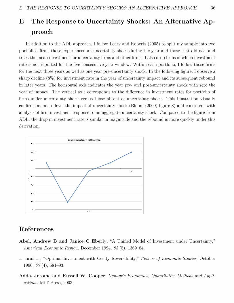
E THE RESPONSE TO UNCERTAINTY SHOCKS: AN ALTERNATIVE APPROACH 36

E The Response to Uncertainty Shocks: An Alternative Ap-proach

In addition to the ADL approach, I follow Leary and Roberts (2005) to split my sample into twoportfolios–firms those experienced an uncertainty shock during the year and those that did not, andtrack the mean investment for uncertainty firms and other firms. I also drop firms of which investmentrate is not reported for the five consecutive year window. Within each portfolio, I follow those firmsfor the next three years as well as one year pre-uncertainty shock. In the following figure, I observe asharp decline (8%) for investment rate in the year of uncertainty impact and its subsequent reboundin later years. The horizontal axis indicates the year pre- and post-uncertainty shock with zero theyear of impact. The vertical axis corresponds to the difference in investment rates for portfolio offirms under uncertainty shock versus those absent of uncertainty shock. This illustration visuallyconfirms at micro-level the impact of uncertainty shock (Bloom (2009) figure 8) and consistent withanalysis of firm investment response to an aggregate uncertainty shock. Compared to the figure fromADL, the drop in investment rate is similar in magnitude and the rebound is more quickly under thisderivation.

��

��

��

��

References

Abel, Andrew B and Janice C Eberly, “A Unified Model of Investment under Uncertainty,”American Economic Review, December 1994, 84 (5), 1369–84.

and , “Optimal Investment with Costly Reversibility,” Review of Economic Studies, October1996, 63 (4), 581–93.

Adda, Jerome and Russell W. Cooper, Dynamic Economics, Quantitative Methods and Appli-cations, MIT Press, 2003.

REFERENCES 37

Almeida, Heitor, Murillo Campello, and Michael S. Weisbach, “The Cash Flow Sensitivityof Cash,” Journal of Finance, 08 2004, 59 (4), 1777–1804.

Arellano, Manuel and Stephen Bond, “Some Tests of Specification for Panel Data: Monte CarloEvidence and an Application to Employment Equations,” The Review of Economic Studies, 1991,58 (2), pp. 277–297.

Athey, Michael J. and Prem S. Laumas, “Internal funds and corporate investment in India,”Journal of Development Economics, December 1994, 45 (2), 287–303.

Baker, Malcolm, Jeremy C. Stein, and Jeffrey Wurgler, “When Does The Market Matter?Stock Prices And The Investment Of Equity-Dependent Firms,” The Quarterly Journal of Eco-nomics, August 2003, 118 (3), 969–1005.

Baum, Christopher F., Mustafa Caglayan, and Oleksandr Talavera, “Uncertainty determi-nants of firm investment,” Economics Letters, March 2008, 98 (3), 282–287.

Bernanke, Ben S., Mark Gertler, and Simon Gilchrist, “The financial accelerator in a quan-titative business cycle framework,” in J. B. Taylor and M. Woodford, eds., Handbook of Macroeco-nomics, Vol. 1 of Handbook of Macroeconomics, Elsevier, April 1999, chapter 21, pp. 1341–1393.

Blanchard, Olivier Jean, Florencio Lopez de Silanes, and Andrei Shleifer, “What do firmsdo with cash windfalls?,” Journal of Financial Economics, December 1994, 36 (3), 337–360.

Bloom, Nicholas, “The Impact of Uncertainty Shocks,” Econometrica, 05 2009, 77 (3), 623–685.

Bloom, Nick, Stephen R. Bond, and John Van Reenen, “Uncertainty and Investment Dy-namics,” Review of Economic Studies, 04 2007, 74 (2), 391–415.

Bolton, Patrick, Hui Chen, and Neng Wang, “A Unified Theory of Tobin’s q, CorporateInvestment, Financing, and Risk Management,” NBER Working Papers 14845, National Bureauof Economic Research, Inc April 2009.

Bond, Stephen R., “Dynamic panel data models: a guide to microdata methods and practice,”CeMMAP working papers CWP09/02, Centre for Microdata Methods and Practice, Institute forFiscal Studies April 2002.

, Alexander Klemm, Rain Newton-Smith, Murtaza Syed, and Gertjan Vlieghe, “Theroles of expected profitability, Tobin’s Q and cash flow in econometric models of company invest-ment,” Bank of England working papers 222, Bank of England June 2004.

and Jason G. Cummins, “Uncertainty and investment: an empirical investigation using data onanalysts’ profits forecasts,” Finance and Economics Discussion Series 2004-20, Board of Governorsof the Federal Reserve System (U.S.) 2004.

REFERENCES 38

Chen, Kaiji, Zheng Song, and Yikai Wang, “Precautionary corporate liquidity,” Working Papersiewwp465, Institute for Empirical Research in Economics January 2010.

Cooper, Russell W. and John C. Haltiwanger, “On the Nature of Capital Adjustment Costs,”Review of Economic Studies, 07 2006, 73 (3), 611–633.

Devereux, Michael and Fabio Schiantarelli, “Investment, Financial Factors, and Cash Flow: Ev-idence from U.K. Panel Data,” in “Asymmetric Information, Corporate Finance, and Investment”NBER Chapters, National Bureau of Economic Research, Inc, 1990, pp. 279–306.

Dixit, Avinash K. and Robert Stephen Pindyck, Investment under uncertainty, Princeton, NJ:Princeton Univ. Press, 1994.

Duke, Elizabeth A., “Small Business Lending, Testimony Before the Committee on FinancialServices and Committee on Small Business, U.S. House of Representatives, Washington, D.C.,”February 26, 2010.

Eisfeldt, Andrea L. and Adriano A. Rampini, “Financing Shortfalls and the Value of AggregateLiquidity,” Working Paper, Duke University August 2009.

Faulkender, Michael and Rong Wang, “Corporate Financial Policy and the Value of Cash,”Journal of Finance, 08 2006, 61 (4), 1957–1990.

Fazzari, Steven M., R. Glenn Hubbard, and Bruce C. Petersen, “Financing Constraints andCorporate Investment,” Brookings Papers on Economic Activity, 1988, 1988 (1), pp. 141–206.

, , and , “Investment-Cash Flow Sensitivities Are Useful: A Comment On Kaplan AndZingales,” The Quarterly Journal of Economics, May 2000, 115 (2), 695–705.

Gilchrist, Simon and Charles P. Himmelberg, “Evidence on the role of cash flow for invest-ment,” Journal of Monetary Economics, December 1995, 36 (3), 541–572.

Gomes, Joao F., “Financing Investment,” American Economic Review, December 2001, 91 (5),1263–1285.

Graham, John R., “How Big Are the Tax Benefits of Debt?,” Journal of Finance, October 2000,55 (5), 1901–1941.

Hadlock, Charles J. and Joshua R. Pierce, “New Evidence on Measuring Financial Constraints:Moving Beyond the KZ Index,” Review of Financial Studies, 2010, 23 (5), 1909–1940.

Hassler, John A. A., “Variations in risk and fluctuations in demand: A theoretical model,” Journalof Economic Dynamics and Control, 1996, 20 (6-7), 1115–1143.

REFERENCES 39

Hayashi, Fumio, “Tobin’s Marginal q and Average q: A Neoclassical Interpretation,” Econometrica,January 1982, 50 (1), 213–24.

Hennessy, Christopher A., Amnon Levy, and Toni M. Whited, “Testing Q theory withfinancing frictions,” Journal of Financial Economics, March 2007, 83 (3), 691–717.

and Toni M. Whited, “How Costly Is External Financing? Evidence from a Structural Esti-mation,” Journal of Finance, 08 2007, 62 (4), 1705–1745.

Holtz-Eakin, Douglas, Whitney Newey, and Harvey S Rosen, “Estimating Vector Autore-gressions with Panel Data,” Econometrica, November 1988, 56 (6), 1371–95.

Jensen, Michael C, “Agency Costs of Free Cash Flow, Corporate Finance, and Takeovers,” Amer-ican Economic Review, May 1986, 76 (2), 323–29.

Judd, Kenneth L., Numerical Methods in Economics, MIT Press, 1998.

Kadapakkam, Palani-Rajan, P. C. Kumar, and Leigh A. Riddick, “The impact of cash flowsand firm size on investment: The international evidence,” Journal of Banking & Finance, March1998, 22 (3), 293–320.

Kaplan, Steven N. and Luigi Zingales, “Do Investment-Cash Flow Sensitivities Provide UsefulMeasures of Financing Constraints,” The Quarterly Journal of Economics, February 1997, 112 (1),169–215.

and , “Investment-Cash Flow Sensitivities Are Not Valid Measures Of Financing Constraints,”The Quarterly Journal of Economics, May 2000, 115 (2), 707–712.

Lamont, Owen, “Cash Flow and Investment: Evidence from Internal Capital Markets,” Journal ofFinance, March 1997, 52 (1), 83–109.

, Christopher Polk, and Jesus Saa-Requejo, “Financial Constraints and Stock Returns,”Review of Financial Studies, 2001, 14 (2), 529–54.

Leahy, John V and Toni M Whited, “The Effect of Uncertainty on Investment: Some StylizedFacts,” Journal of Money, Credit and Banking, February 1996, 28 (1), 64–83.

Leary, Mark T. and Michael R. Roberts, “Do Firms Rebalance Their Capital Structures?,”Journal of Finance, December 2005, 60 (6), 2575–2619.

Livdan, Dmitry, Horacio Sapriza, and Lu Zhang, “Financially Constrained Stock Returns,”Journal of Finance, 08 2009, 64 (4), 1827–1862.

Lucas, Robert E. and Nancy L. Stokey, Recursive Methods in Economic Dynamics, HarvardUniversity Press, 1989.

REFERENCES 40

Malmendier, Ulrike and Geoffrey Tate, “CEO Overconfidence and Corporate Investment,”Journal of Finance, 02 2005, 60 (6), 2661–2700.

Miller, Merton H. and Franco Modigliani, “Dividend Policy, Growth, and the Valuation ofShares,” Journal of Business, 1961, 34, 411.

Modigliani, Franco and Merton H. Miller, “The Cost of Capital, Corporation Finance and theTheory of Investment,” The American Economic Review, 1958, 48 (3), pp. 261–297.

Petersen, Mitchell A. and Raghuram G. Rajan, “The Benefits of Lending Relationships: Evi-dence from Small Business Data,” The Journal of Finance, 1994, 49 (1), pp. 3–37.

Riddick, Leigh A. and Toni M. Whited, “The Corporate Propensity to Save,” Journal of Fi-nance, 08 2009, 64 (4), 1729–1766.

Salinger, Michael and Lawrence H. Summers, “Tax Reform and Corporate Investment: AMicroeconometric Simulation Study,” in “Behavioral Simulation Methods in Tax Policy Analysis”NBER Chapters, National Bureau of Economic Research, Inc, 1983, pp. 247–288.

Tauchen, George, “Finite state markov-chain approximations to univariate and vector autoregres-sions,” Economics Letters, 1986, 20 (2), 177–181.

and Robert Hussey, “Quadrature-Based Methods for Obtaining Approximate Solutions toNonlinear Asset Pricing Models,” Econometrica, March 1991, 59 (2), 371–96.

Whited, Toni M., “Debt, Liquidity Constraints, and Corporate Investment: Evidence from PanelData,” Journal of Finance, September 1992, 47 (4), 1425–60.

, “External finance constraints and the intertemporal pattern of intermittent investment,” Journalof Financial Economics, September 2006, 81 (3), 467–502.

and Guojun Wu, “Financial Constraints Risk,” Review of Financial Studies, 2006, 19 (2), 531–559.

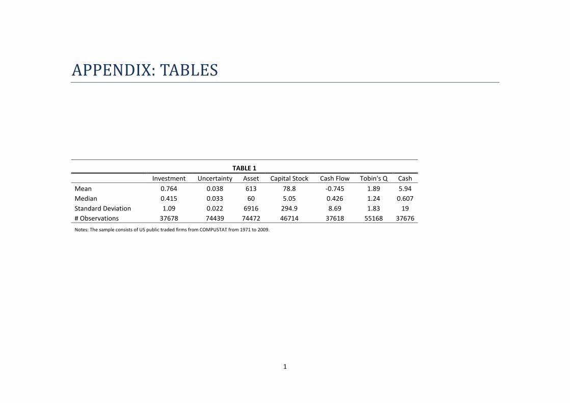
1

APPENDIX: TABLES

TABLE 1 Investment Uncertainty Asset Capital Stock Cash Flow Tobin's Q Cash Mean 0.764 0.038 613 78.8 ‐0.745 1.89 5.94 Median 0.415 0.033 60 5.05 0.426 1.24 0.607 Standard Deviation 1.09 0.022 6916 294.9 8.69 1.83 19 # Observations 37678 74439 74472 46714 37618 55168 37676

Notes: The sample consists of US public traded firms from COMPUSTAT from 1971 to 2009.

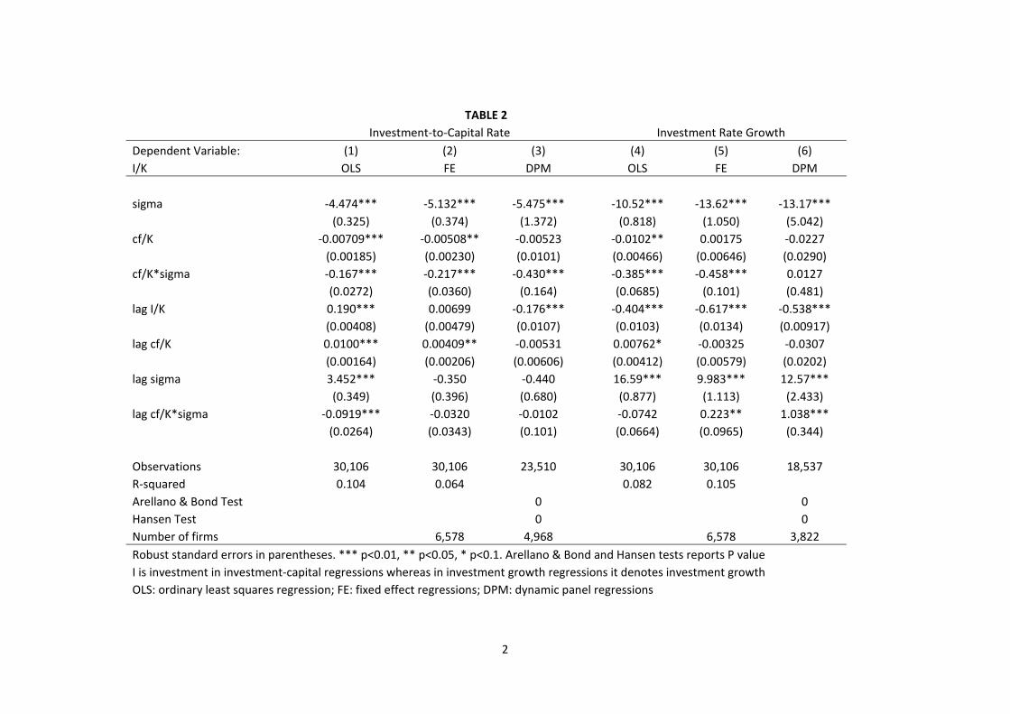
2

TABLE 2 Investment‐to‐Capital Rate Investment Rate Growth

Dependent Variable: (1) (2) (3) (4) (5) (6) I/K OLS FE DPM OLS FE DPM sigma ‐4.474*** ‐5.132*** ‐5.475*** ‐10.52*** ‐13.62*** ‐13.17***

(0.325) (0.374) (1.372) (0.818) (1.050) (5.042) cf/K ‐0.00709*** ‐0.00508** ‐0.00523 ‐0.0102** 0.00175 ‐0.0227

(0.00185) (0.00230) (0.0101) (0.00466) (0.00646) (0.0290) cf/K*sigma ‐0.167*** ‐0.217*** ‐0.430*** ‐0.385*** ‐0.458*** 0.0127

(0.0272) (0.0360) (0.164) (0.0685) (0.101) (0.481) lag I/K 0.190*** 0.00699 ‐0.176*** ‐0.404*** ‐0.617*** ‐0.538***

(0.00408) (0.00479) (0.0107) (0.0103) (0.0134) (0.00917) lag cf/K 0.0100*** 0.00409** ‐0.00531 0.00762* ‐0.00325 ‐0.0307

(0.00164) (0.00206) (0.00606) (0.00412) (0.00579) (0.0202) lag sigma 3.452*** ‐0.350 ‐0.440 16.59*** 9.983*** 12.57***

(0.349) (0.396) (0.680) (0.877) (1.113) (2.433) lag cf/K*sigma ‐0.0919*** ‐0.0320 ‐0.0102 ‐0.0742 0.223** 1.038***

(0.0264) (0.0343) (0.101) (0.0664) (0.0965) (0.344)

Observations 30,106 30,106 23,510 30,106 30,106 18,537 R‐squared 0.104 0.064 0.082 0.105 Arellano & Bond Test 0 0 Hansen Test 0 0 Number of firms 6,578 4,968 6,578 3,822 Robust standard errors in parentheses. *** p<0.01, ** p<0.05, * p<0.1. Arellano & Bond and Hansen tests reports P value I is investment in investment‐capital regressions whereas in investment growth regressions it denotes investment growth OLS: ordinary least squares regression; FE: fixed effect regressions; DPM: dynamic panel regressions

3

TABLE 3

Asset Percentiles: 0‐10% 10%‐20% 20%‐30% 30%‐40% 40%‐50% 50%‐60% 60%‐70% 70%‐80% 80%‐90% 90%‐100%

I/K mean 0.785 0.789 0.757 0.742 0.796 0.783 0.756 0.774 0.735 0.680 standard deviation 1.315 1.224 1.167 1.084 1.110 1.123 0.941 0.933 0.920 0.706 sigma mean 0.052 0.047 0.044 0.042 0.039 0.037 0.034 0.032 0.029 0.025 standard deviation 0.027 0.026 0.024 0.022 0.020 0.020 0.018 0.016 0.016 0.012 cf/K mean ‐3.610 ‐1.295 ‐1.151 ‐0.941 ‐0.454 ‐0.636 0.066 0.642 0.968 0.910 standard deviation 12.466 10.287 9.327 9.424 8.376 8.467 6.967 4.752 3.543 2.365 Asset mean 5 14 26 40 62 103 157 289 645 4794 standard deviation 7 23 58 48 76 185 224 332 766 5432

4

TABLE 4A: OLS Dependent Variable: (1) (2) (3) (4) (5) (6) (7) (8) (9) (10) I/K 0‐10% 10%‐20% 20%‐30% 30%‐40% 40%‐50% 50%‐60% 60%‐70% 70%‐80% 80%‐90% 90%‐100% sigma ‐4.804*** ‐4.930*** ‐4.093*** ‐4.533*** ‐7.702*** ‐3.577*** ‐3.611*** ‐3.634*** ‐1.104 ‐1.787

(0.845) (0.936) (0.943) (1.001) (1.221) (1.188) (1.050) (1.193) (1.375) (1.109) cf/K ‐0.0227*** ‐0.00181 0.00128 ‐0.0234*** ‐0.00106 0.0169** 0.00813 0.0108 0.0195* 0.110***

(0.00430) (0.00590) (0.00540) (0.00547) (0.00761) (0.00660) (0.00747) (0.0106) (0.0103) (0.0116) cf/K*sigma 0.0450 ‐0.359*** ‐0.220** ‐0.103 ‐0.286** ‐0.514*** ‐0.0163 ‐0.199 0.105 ‐1.455***

(0.0549) (0.0860) (0.0859) (0.0829) (0.139) (0.111) (0.156) (0.219) (0.197) (0.286) lag I/K 0.101*** 0.158*** 0.163*** 0.219*** 0.161*** 0.217*** 0.266*** 0.249*** 0.275*** 0.311***

(0.0120) (0.0123) (0.0114) (0.0127) (0.0140) (0.0127) (0.0121) (0.0133) (0.0150) (0.0124) lag cf/K 0.0109*** 0.00857* 0.00518 0.0153*** 0.0113* 0.0173*** ‐0.00593 0.00496 0.0740*** ‐0.0270***

(0.00385) (0.00507) (0.00492) (0.00550) (0.00651) (0.00564) (0.00598) (0.00786) (0.0123) (0.00957) lag sigma 1.874** 1.670* 2.326** 2.427** 7.564*** 3.063** 2.527** 7.206*** 3.988*** 4.707***

(0.923) (0.997) (1.007) (1.059) (1.311) (1.305) (1.130) (1.318) (1.538) (1.207) lag cf/K*sigma ‐0.148*** ‐0.0130 0.0265 ‐0.0903 ‐0.305*** ‐0.363*** ‐0.0105 ‐0.0911 ‐1.786*** 0.602***

(0.0538) (0.0797) (0.0793) (0.0979) (0.118) (0.106) (0.125) (0.153) (0.289) (0.214)

Observations 3,661 3,704 3,469 3,319 3,082 2,995 2,707 2,582 2,391 2,196 R‐squared 0.078 0.104 0.087 0.151 0.117 0.153 0.210 0.168 0.202 0.390 Standard errors in parentheses *** p<0.01, ** p<0.05, * p<0.1

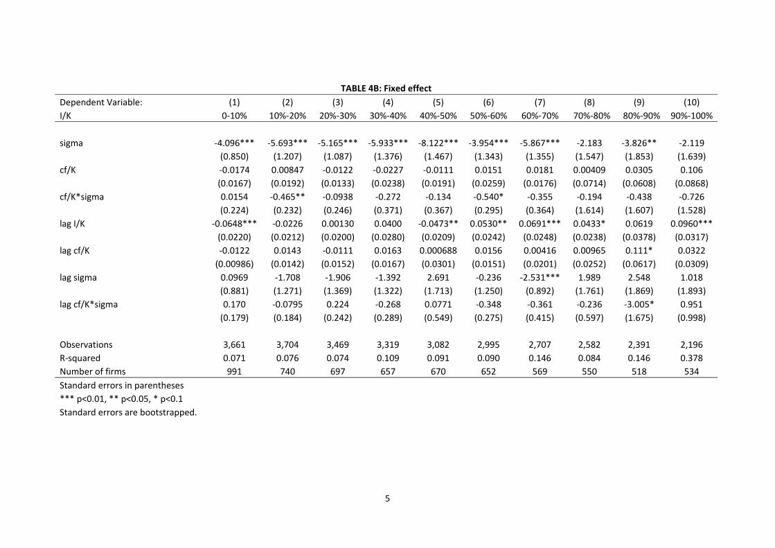
5

TABLE 4B: Fixed effect Dependent Variable: (1) (2) (3) (4) (5) (6) (7) (8) (9) (10) I/K 0‐10% 10%‐20% 20%‐30% 30%‐40% 40%‐50% 50%‐60% 60%‐70% 70%‐80% 80%‐90% 90%‐100% sigma ‐4.096*** ‐5.693*** ‐5.165*** ‐5.933*** ‐8.122*** ‐3.954*** ‐5.867*** ‐2.183 ‐3.826** ‐2.119

(0.850) (1.207) (1.087) (1.376) (1.467) (1.343) (1.355) (1.547) (1.853) (1.639) cf/K ‐0.0174 0.00847 ‐0.0122 ‐0.0227 ‐0.0111 0.0151 0.0181 0.00409 0.0305 0.106

(0.0167) (0.0192) (0.0133) (0.0238) (0.0191) (0.0259) (0.0176) (0.0714) (0.0608) (0.0868) cf/K*sigma 0.0154 ‐0.465** ‐0.0938 ‐0.272 ‐0.134 ‐0.540* ‐0.355 ‐0.194 ‐0.438 ‐0.726

(0.224) (0.232) (0.246) (0.371) (0.367) (0.295) (0.364) (1.614) (1.607) (1.528) lag I/K ‐0.0648*** ‐0.0226 0.00130 0.0400 ‐0.0473** 0.0530** 0.0691*** 0.0433* 0.0619 0.0960***

(0.0220) (0.0212) (0.0200) (0.0280) (0.0209) (0.0242) (0.0248) (0.0238) (0.0378) (0.0317) lag cf/K ‐0.0122 0.0143 ‐0.0111 0.0163 0.000688 0.0156 0.00416 0.00965 0.111* 0.0322

(0.00986) (0.0142) (0.0152) (0.0167) (0.0301) (0.0151) (0.0201) (0.0252) (0.0617) (0.0309) lag sigma 0.0969 ‐1.708 ‐1.906 ‐1.392 2.691 ‐0.236 ‐2.531*** 1.989 2.548 1.018

(0.881) (1.271) (1.369) (1.322) (1.713) (1.250) (0.892) (1.761) (1.869) (1.893) lag cf/K*sigma 0.170 ‐0.0795 0.224 ‐0.268 0.0771 ‐0.348 ‐0.361 ‐0.236 ‐3.005* 0.951

(0.179) (0.184) (0.242) (0.289) (0.549) (0.275) (0.415) (0.597) (1.675) (0.998)

Observations 3,661 3,704 3,469 3,319 3,082 2,995 2,707 2,582 2,391 2,196 R‐squared 0.071 0.076 0.074 0.109 0.091 0.090 0.146 0.084 0.146 0.378 Number of firms 991 740 697 657 670 652 569 550 518 534 Standard errors in parentheses *** p<0.01, ** p<0.05, * p<0.1 Standard errors are bootstrapped.

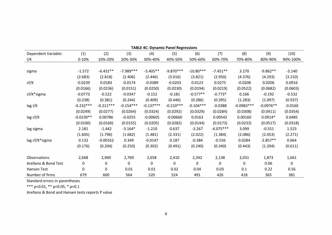
6

TABLE 4C: Dynamic Panel Regressions Dependent Variable: (1) (2) (3) (4) (5) (6) (7) (8) (9) (10) I/K 0‐10% 10%‐20% 20%‐30% 30%‐40% 40%‐50% 50%‐60% 60%‐70% 70%‐80% 80%‐90% 90%‐100% sigma ‐1.572 ‐6.431** ‐7.989*** ‐5.405** ‐9.870*** ‐10.80*** ‐7.451** 3.270 ‐9.862** ‐3.140

(2.683) (2.818) (2.406) (2.446) (3.016) (3.821) (2.950) (4.376) (4.293) (3.210) cf/K ‐0.0239 0.0183 ‐0.0174 ‐0.0389 ‐0.0203 0.0123 0.0275 ‐0.0208 0.0206 0.0916

(0.0166) (0.0236) (0.0151) (0.0250) (0.0230) (0.0194) (0.0219) (0.0522) (0.0682) (0.0603) cf/K*sigma ‐0.0773 ‐0.522 ‐0.0347 ‐0.152 ‐0.181 ‐0.577** ‐0.773* 0.166 ‐0.192 ‐0.532

(0.238) (0.381) (0.244) (0.409) (0.446) (0.286) (0.395) (1.283) (1.097) (0.937) lag I/K ‐0.232*** ‐0.211*** ‐0.154*** ‐0.137*** ‐0.210*** ‐0.104*** ‐0.0388 ‐0.0983*** ‐0.0976** ‐0.0160

(0.0249) (0.0277) (0.0264) (0.0324) (0.0292) (0.0329) (0.0284) (0.0308) (0.0411) (0.0354) lag cf/K ‐0.0230** 0.00786 ‐0.0255 ‐0.00605 ‐0.00660 0.0163 0.00542 0.00160 0.0914* 0.0485

(0.0100) (0.0160) (0.0155) (0.0205) (0.0282) (0.0144) (0.0173) (0.0233) (0.0517) (0.0318) lag sigma 2.181 ‐1.442 ‐3.164* ‐1.210 0.637 ‐3.267 ‐4.075*** 3.099 ‐0.551 1.523

(1.605) (1.796) (1.682) (1.481) (2.331) (2.022) (1.384) (2.086) (2.053) (2.271) lag cf/K*sigma 0.132 ‐0.00162 0.349 ‐0.0147 0.187 ‐0.384 ‐0.556 0.0284 ‐2.857** 0.664

(0.176) (0.204) (0.250) (0.302) (0.491) (0.240) (0.340) (0.443) (1.204) (0.611)

Observations 2,668 2,960 2,769 2,658 2,410 2,342 2,138 2,031 1,873 1,661 Arellano & Bond Test 0 0 0 0 0 0 0 0 0.06 0 Hansen Test 0 0 0.01 0.01 0.02 0.04 0.03 0.1 0.22 0.56 Number of firms 679 600 564 520 524 491 426 418 365 381 Standard errors in parentheses *** p<0.01, ** p<0.05, * p<0.1 Arellano & Bond and Hansen tests reports P value

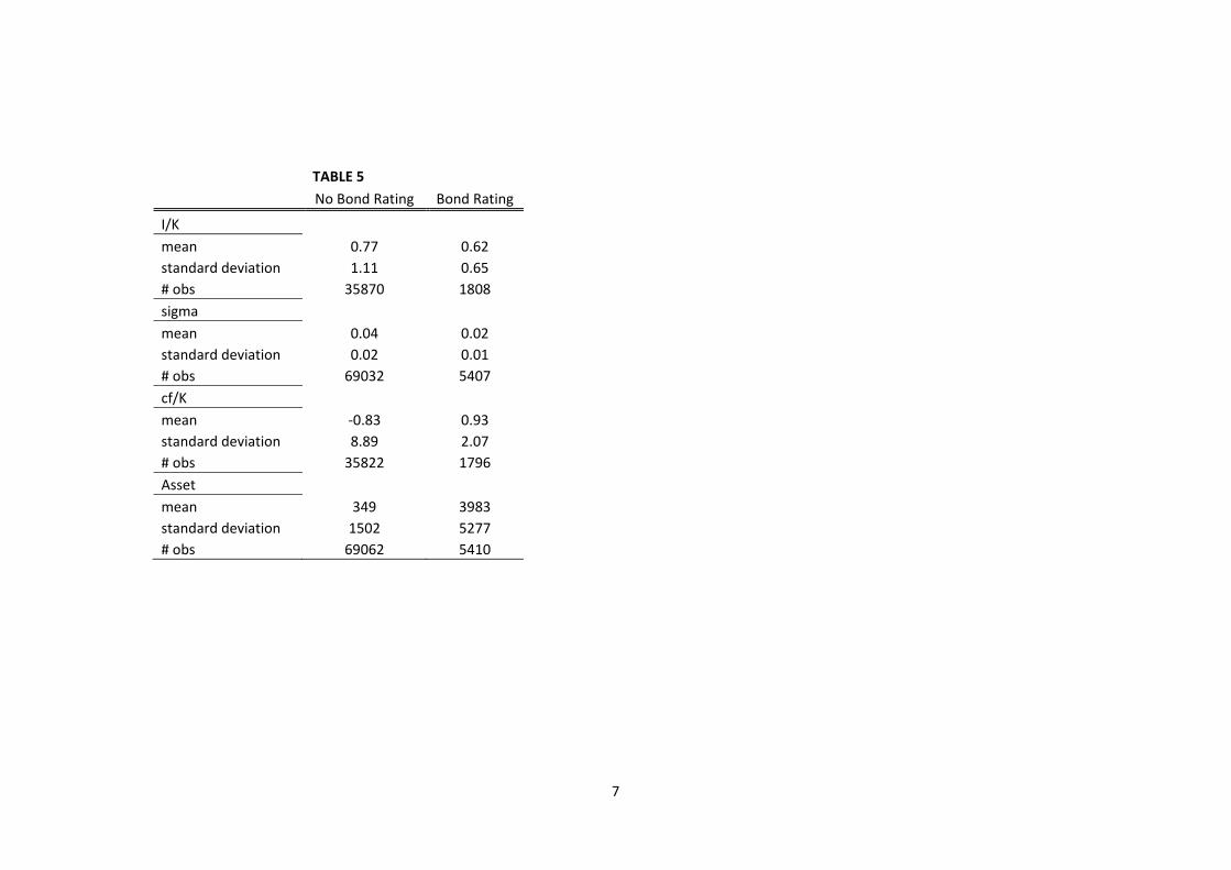
7

TABLE 5

No Bond Rating Bond Rating

I/K mean 0.77 0.62 standard deviation 1.11 0.65 # obs 35870 1808 sigma mean 0.04 0.02 standard deviation 0.02 0.01 # obs 69032 5407 cf/K mean ‐0.83 0.93 standard deviation 8.89 2.07 # obs 35822 1796 Asset mean 349 3983 standard deviation 1502 5277 # obs 69062 5410

8

TABLE 6 OLS Fixed Effect Dynamic Panel

Dependent Variable: (1) (2) (3) (4) (5) (6) I/K Unrated Rated Unrated Rated Unrated Rated sigma ‐4.565*** 0.718 ‐5.088*** ‐0.799 ‐6.678*** ‐6.760

(0.338) (3.257) (0.349) (2.089) (1.420) (5.107) cf/K ‐0.00798 0.182*** ‐0.00574 0.183 ‐0.0162 0.239**

(0.00604) (0.0609) (0.00730) (0.130) (0.0141) (0.0961)cf/K*sigma ‐0.159* ‐1.146* ‐0.210* ‐2.363 ‐0.157 ‐2.702

(0.0863) (0.612) (0.118) (3.040) (0.221) (1.740) lag I/K 0.187*** 0.304*** 0.00409 0.0386 ‐0.183*** 0.0574

(0.00735) (0.0450) (0.00578) (0.0972) (0.0114) (0.0458)lag cf/K 0.00999** ‐0.0245 0.00385 0.0696 0.00575 0.0780

(0.00471) (0.0587) (0.00537) (0.106) (0.00715) (0.0763)lag sigma 3.311*** 4.276 ‐0.413 1.248 ‐1.178* 0.314

(0.421) (3.443) (0.528) (2.031) (0.683) (1.935) lag cf/K*sigma ‐0.0906 0.113 ‐0.0298 ‐0.205 ‐0.126 ‐0.349

(0.0842) (1.196) (0.0917) (1.785) (0.118) (1.293)

Observations 28,636 1,470 28,636 1,470 20,911 1,118 R‐squared 0.103 0.382 0.064 0.314 Arellano & Bond Test 0 0.02 Hansen Test 0 1 Number of firms 6,345 348 4,530 252 Robust standard errors in parentheses. *** p<0.01, ** p<0.05, * p<0.1 Arellano & Bond and Hansen tests reports P value

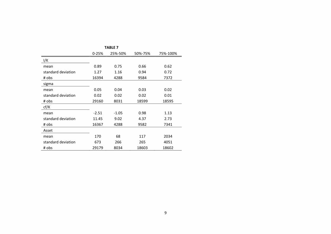
9

TABLE 7

0‐25% 25%‐50% 50%‐75% 75%‐100%

I/K mean 0.89 0.75 0.66 0.62 standard deviation 1.27 1.16 0.94 0.72 # obs 16394 4288 9584 7372 sigma mean 0.05 0.04 0.03 0.02 standard deviation 0.02 0.02 0.02 0.01 # obs 29160 8031 18599 18595 cf/K mean ‐2.51 ‐1.05 0.98 1.13 standard deviation 11.45 9.02 4.37 2.73 # obs 16367 4288 9582 7341 Asset mean 170 68 117 2034 standard deviation 673 266 265 4051 # obs 29179 8034 18603 18602

10

TABLE 8A: OLS Dependent Variable: I/K (1) (2) (3) (4)

0‐25% 25%‐50% 50%‐75% 75%‐100% sigma ‐6.206*** ‐5.309*** ‐1.411* ‐0.830

(0.448) (0.898) (0.833) (0.909) cf/K ‐0.0111* ‐0.0266 0.0640*** 0.148***

(0.00664) (0.0188) (0.0237) (0.0403) cf/K*sigma ‐0.113 ‐0.0591 ‐0.945** ‐1.945***

(0.0942) (0.280) (0.394) (0.633) lag I/K 0.169*** 0.133*** 0.212*** 0.243***

(0.00956) (0.0159) (0.0207) (0.0203) lag cf/K 0.0104* 0.00926 0.000818 0.00763

(0.00557) (0.0100) (0.0146) (0.0173) lag sigma 1.783*** 1.960** 2.498*** 3.860***

(0.578) (0.904) (0.960) (0.932) lag cf/K*sigma ‐0.105 ‐0.133 0.156 ‐0.878**

(0.0990) (0.164) (0.220) (0.371)

Observations 12,476 3,560 8,033 6,010 R‐squared 0.097 0.132 0.148 0.282 Number of firms Robust standard errors in parentheses *** p<0.01, ** p<0.05, * p<0.1

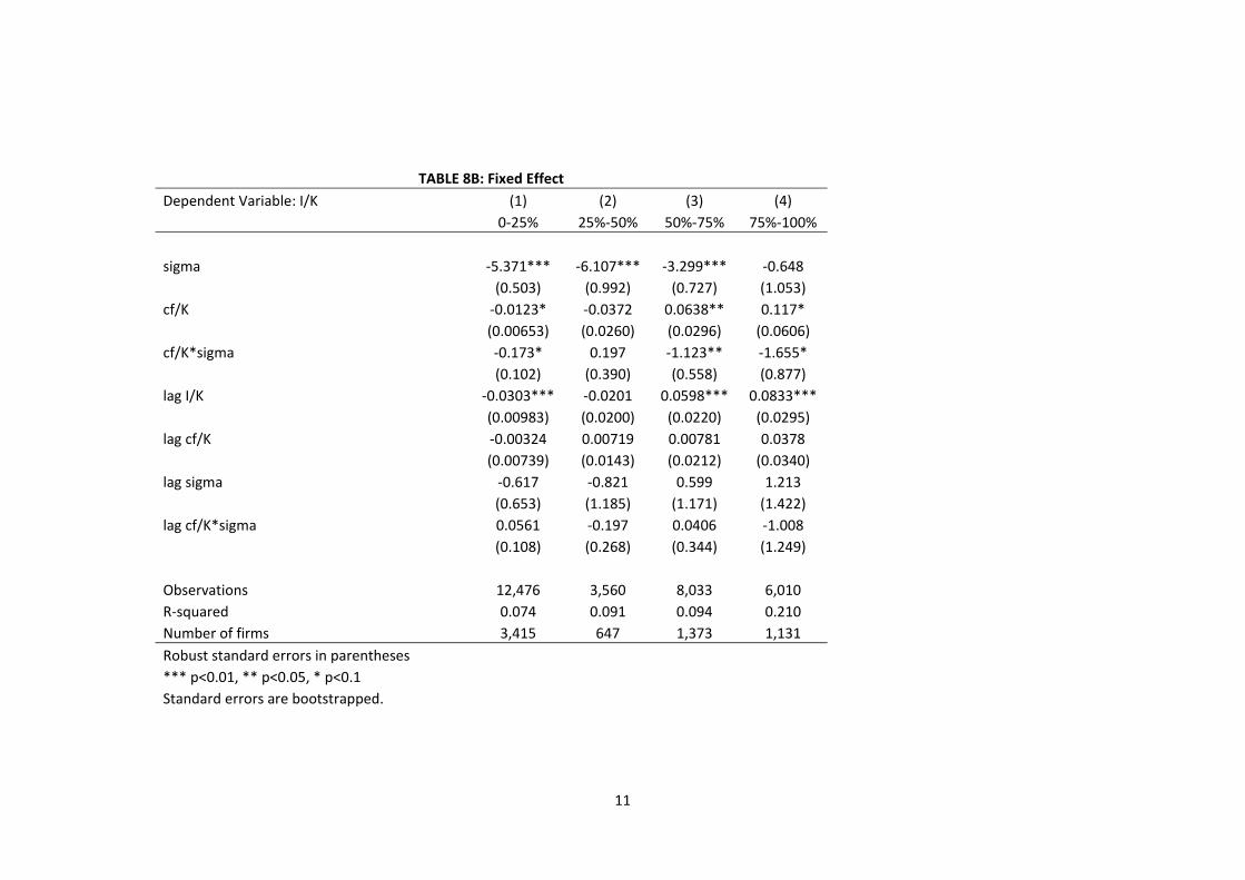
11

TABLE 8B: Fixed Effect Dependent Variable: I/K (1) (2) (3) (4)

0‐25% 25%‐50% 50%‐75% 75%‐100% sigma ‐5.371*** ‐6.107*** ‐3.299*** ‐0.648

(0.503) (0.992) (0.727) (1.053) cf/K ‐0.0123* ‐0.0372 0.0638** 0.117*

(0.00653) (0.0260) (0.0296) (0.0606) cf/K*sigma ‐0.173* 0.197 ‐1.123** ‐1.655*

(0.102) (0.390) (0.558) (0.877) lag I/K ‐0.0303*** ‐0.0201 0.0598*** 0.0833***

(0.00983) (0.0200) (0.0220) (0.0295) lag cf/K ‐0.00324 0.00719 0.00781 0.0378

(0.00739) (0.0143) (0.0212) (0.0340) lag sigma ‐0.617 ‐0.821 0.599 1.213

(0.653) (1.185) (1.171) (1.422) lag cf/K*sigma 0.0561 ‐0.197 0.0406 ‐1.008

(0.108) (0.268) (0.344) (1.249)

Observations 12,476 3,560 8,033 6,010 R‐squared 0.074 0.091 0.094 0.210 Number of firms 3,415 647 1,373 1,131 Robust standard errors in parentheses *** p<0.01, ** p<0.05, * p<0.1 Standard errors are bootstrapped.

12

TABLE 8C: Dynamic Panel Dependent Variable: I/K (1) (2) (3) (4)

0‐25% 25%‐50% 50%‐75% 75%‐100% sigma ‐0.645 ‐9.395*** ‐9.000*** 1.108

(1.821) (2.900) (1.973) (2.647) cf/K ‐0.0200* ‐0.0457* 0.107*** 0.101*

(0.0112) (0.0271) (0.0325) (0.0573) cf/K*sigma ‐0.336** 0.215 ‐1.911*** ‐1.271

(0.168) (0.404) (0.626) (0.886) lag I/K ‐0.220*** ‐0.156*** ‐0.120*** ‐0.0395

(0.0151) (0.0281) (0.0225) (0.0261) lag cf/K ‐0.0152** 0.000623 0.0261 0.0457**

(0.00680) (0.0132) (0.0218) (0.0230) lag sigma 1.199 ‐2.213 ‐1.418 1.863

(0.965) (1.961) (1.360) (1.479) lag cf/K*sigma 0.0964 ‐0.180 ‐0.483 ‐0.825***

(0.118) (0.219) (0.343) (0.293)

Observations 9,049 2,913 6,657 4,876 Arellano & Bond Test 0 0 0 0 Hansen Test 0 0 0 0 Number of firms 2,388 546 1,145 882 Robust standard errors in parentheses *** p<0.01, ** p<0.05, * p<0.1 Arellano & Bond and Hansen tests reports P value

13

TABLE 9

Asset Percentiles: 0‐10% 10%‐20% 20%‐30% 30%‐40% 40%‐50% 50%‐60% 60%‐70% 70%‐80% 80%‐90% 90%‐100%

I/K mean 0.61 0.69 0.76 0.78 0.77 0.78 0.80 0.79 0.77 0.83 standard deviation 0.87 0.90 1.01 1.01 1.06 1.11 1.15 1.13 1.18 1.30 sigma mean 0.03 0.03 0.04 0.04 0.04 0.04 0.04 0.04 0.04 0.05 standard deviation 0.01 0.02 0.02 0.02 0.02 0.02 0.02 0.02 0.02 0.03 cf/K mean 1.88 1.18 0.70 0.41 ‐0.37 ‐0.95 ‐0.90 ‐1.64 ‐1.85 ‐5.20 standard deviation 3.56 5.05 6.16 6.76 8.27 8.04 8.29 10.04 9.75 13.70 Asset mean 1086 634 517 634 785 471 574 467 461 446 standard deviation 3520 2302 1869 2156 2567 1745 2044 1648 1653 1959

14

TABLE 10A: OLS Dependent Variable: (1) (2) (3) (4) (5) (6) (7) (8) (9) (10) I/K 0‐10% 10%‐20% 20%‐30% 30%‐40% 40%‐50% 50%‐60% 60%‐70% 70%‐80% 80%‐90% 90%‐100% sigma 1.938 ‐3.114** ‐2.411** ‐3.220*** ‐5.011*** ‐3.381*** ‐5.586*** ‐5.394*** ‐5.266*** ‐4.637***

(1.445) (1.502) (1.088) (0.988) (1.307) (1.308) (1.209) (1.086) (0.835) (0.735) cf/K 0.197*** 0.0276 0.0211 0.00842 ‐0.0246 0.0270 ‐0.00298 0.00183 ‐0.0204 ‐0.0452***

(0.0369) (0.0205) (0.0242) (0.0410) (0.0191) (0.0226) (0.0155) (0.0134) (0.0207) (0.0111) cf/K*sigma ‐2.640*** ‐0.219 ‐0.119 ‐0.275 ‐0.112 ‐0.455 ‐0.244 ‐0.381** ‐0.138 0.242*

(0.811) (0.291) (0.327) (0.636) (0.348) (0.381) (0.254) (0.192) (0.216) (0.141) lag I/K 0.150*** 0.243*** 0.196*** 0.181*** 0.211*** 0.179*** 0.182*** 0.249*** 0.162*** 0.142***

(0.0306) (0.0339) (0.0239) (0.0241) (0.0241) (0.0203) (0.0208) (0.0235) (0.0210) (0.0188) lag cf/K ‐0.0427 0.0177 0.0323* 0.0459** 0.0227 0.00324 0.0129 ‐0.00716 ‐0.00131 0.0148*

(0.0262) (0.0184) (0.0172) (0.0209) (0.0149) (0.0142) (0.0167) (0.0122) (0.0123) (0.00836) lag sigma 0.406 6.499*** 2.427* 2.398** 4.325*** 1.814 5.031*** 2.895** 2.251** 1.419

(1.286) (2.024) (1.260) (1.054) (1.663) (1.390) (1.479) (1.156) (1.031) (1.082) lag cf/K*sigma 0.836 ‐0.511 ‐0.412 ‐0.709** ‐0.258 ‐0.203 ‐0.135 0.217 0.229 ‐0.149

(0.535) (0.394) (0.299) (0.358) (0.249) (0.264) (0.320) (0.180) (0.162) (0.136)

Observations 3,066 2,909 2,707 2,710 2,874 2,990 3,073 2,980 3,058 2,980 R‐squared 0.284 0.195 0.137 0.109 0.162 0.104 0.115 0.175 0.124 0.165 Standard errors in parentheses *** p<0.01, ** p<0.05, * p<0.1

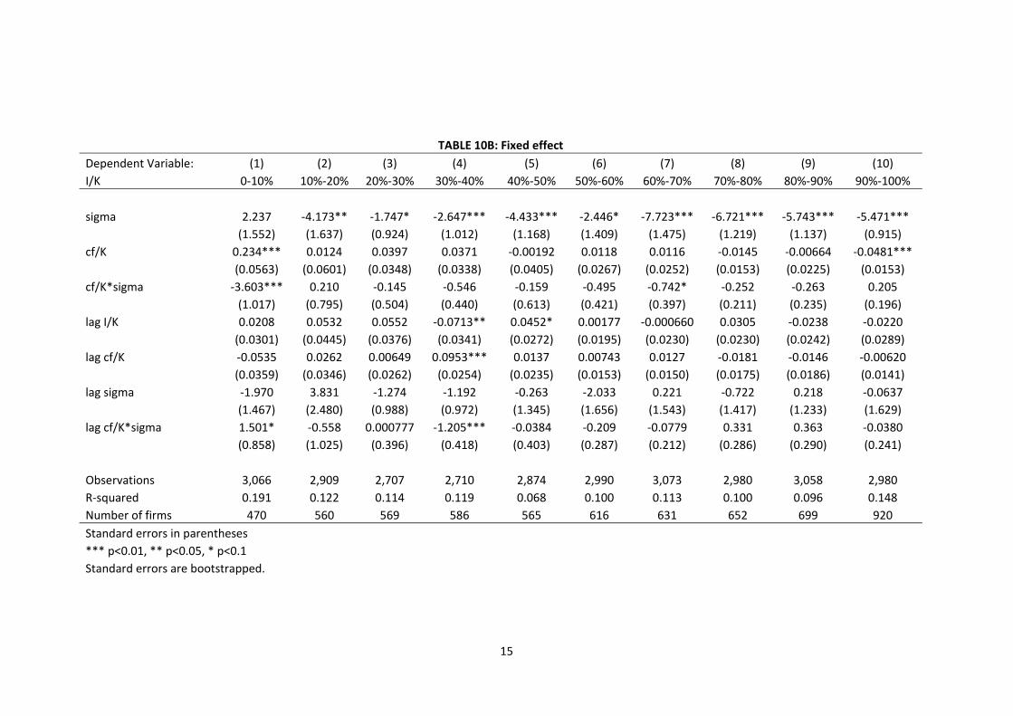
15

TABLE 10B: Fixed effect Dependent Variable: (1) (2) (3) (4) (5) (6) (7) (8) (9) (10) I/K 0‐10% 10%‐20% 20%‐30% 30%‐40% 40%‐50% 50%‐60% 60%‐70% 70%‐80% 80%‐90% 90%‐100% sigma 2.237 ‐4.173** ‐1.747* ‐2.647*** ‐4.433*** ‐2.446* ‐7.723*** ‐6.721*** ‐5.743*** ‐5.471***

(1.552) (1.637) (0.924) (1.012) (1.168) (1.409) (1.475) (1.219) (1.137) (0.915) cf/K 0.234*** 0.0124 0.0397 0.0371 ‐0.00192 0.0118 0.0116 ‐0.0145 ‐0.00664 ‐0.0481***

(0.0563) (0.0601) (0.0348) (0.0338) (0.0405) (0.0267) (0.0252) (0.0153) (0.0225) (0.0153) cf/K*sigma ‐3.603*** 0.210 ‐0.145 ‐0.546 ‐0.159 ‐0.495 ‐0.742* ‐0.252 ‐0.263 0.205

(1.017) (0.795) (0.504) (0.440) (0.613) (0.421) (0.397) (0.211) (0.235) (0.196) lag I/K 0.0208 0.0532 0.0552 ‐0.0713** 0.0452* 0.00177 ‐0.000660 0.0305 ‐0.0238 ‐0.0220

(0.0301) (0.0445) (0.0376) (0.0341) (0.0272) (0.0195) (0.0230) (0.0230) (0.0242) (0.0289) lag cf/K ‐0.0535 0.0262 0.00649 0.0953*** 0.0137 0.00743 0.0127 ‐0.0181 ‐0.0146 ‐0.00620

(0.0359) (0.0346) (0.0262) (0.0254) (0.0235) (0.0153) (0.0150) (0.0175) (0.0186) (0.0141) lag sigma ‐1.970 3.831 ‐1.274 ‐1.192 ‐0.263 ‐2.033 0.221 ‐0.722 0.218 ‐0.0637

(1.467) (2.480) (0.988) (0.972) (1.345) (1.656) (1.543) (1.417) (1.233) (1.629) lag cf/K*sigma 1.501* ‐0.558 0.000777 ‐1.205*** ‐0.0384 ‐0.209 ‐0.0779 0.331 0.363 ‐0.0380

(0.858) (1.025) (0.396) (0.418) (0.403) (0.287) (0.212) (0.286) (0.290) (0.241)

Observations 3,066 2,909 2,707 2,710 2,874 2,990 3,073 2,980 3,058 2,980 R‐squared 0.191 0.122 0.114 0.119 0.068 0.100 0.113 0.100 0.096 0.148 Number of firms 470 560 569 586 565 616 631 652 699 920 Standard errors in parentheses *** p<0.01, ** p<0.05, * p<0.1 Standard errors are bootstrapped.

16

TABLE 10C: Dynamic Panel Dependent Variable: (1) (2) (3) (4) (5) (6) (7) (8) (9) (10) I/K 0‐10% 10%‐20% 20%‐30% 30%‐40% 40%‐50% 50%‐60% 60%‐70% 70%‐80% 80%‐90% 90%‐100% sigma ‐0.796 ‐4.631* ‐1.788 ‐3.032 ‐7.272** ‐2.231 ‐10.28*** ‐8.484*** ‐7.324** ‐8.260***

(2.668) (2.431) (2.549) (2.207) (3.461) (3.792) (3.260) (2.989) (3.713) (2.854) cf/K 0.229*** 0.0691 0.0391 0.0237 ‐0.0202 0.00606 0.0121 ‐0.0418** 0.00406 ‐0.0446***

(0.0736) (0.0491) (0.0328) (0.0371) (0.0287) (0.0273) (0.0195) (0.0188) (0.0240) (0.0151) cf/K*sigma ‐3.648*** ‐0.750 ‐0.243 ‐0.503 0.0520 ‐0.481 ‐0.779*** 0.160 ‐0.619** ‐0.117

(1.397) (0.909) (0.488) (0.475) (0.341) (0.502) (0.295) (0.228) (0.255) (0.229) lag I/K ‐0.132*** ‐0.117*** ‐0.0735 ‐0.190*** ‐0.135*** ‐0.173*** ‐0.191*** ‐0.140*** ‐0.153*** ‐0.188***

(0.0426) (0.0323) (0.0464) (0.0308) (0.0387) (0.0301) (0.0315) (0.0312) (0.0308) (0.0300) lag cf/K ‐0.0329 0.0578 ‐0.00511 0.0906*** ‐0.00623 0.0142 0.0117 ‐0.0359** ‐0.0216 ‐0.0210**

(0.0398) (0.0364) (0.0259) (0.0294) (0.0250) (0.0153) (0.0160) (0.0140) (0.0214) (0.00963) lag sigma ‐3.362** 4.125 ‐1.729 ‐1.008 ‐1.208 ‐3.777* ‐1.617 ‐1.986 0.120 ‐1.000

(1.647) (3.043) (1.843) (1.264) (2.159) (2.275) (1.971) (1.598) (1.896) (1.979) lag cf/K*sigma 1.501* ‐1.006 0.102 ‐1.158** 0.148 ‐0.310 ‐0.200 0.587** 0.339 ‐0.00220

(0.906) (0.925) (0.435) (0.450) (0.356) (0.289) (0.206) (0.229) (0.309) (0.192)

Observations 2,594 2,348 2,137 2,121 2,308 2,372 2,440 2,327 2,359 2,056 Arellano & Bond Test 0 0 0 0 0 0 0 0.02 0.01 0 Hansen Test 0.3 0.1 0.04 0.04 0.03 0.03 0.05 0.03 0.03 0.01 Number of firms 385 445 441 448 437 483 492 514 528 606 Standard errors in parentheses *** p<0.01, ** p<0.05, * p<0.1 Arellano & Bond and Hansen tests reports P value

uncertainty and financially constrained investment: theory

Documents