chance constrained optimal power flow: …dano/papers/cc-opf3.pdfchance constrained optimal power...

CHANCE CONSTRAINED OPTIMAL POWER FLOW:RISK-AWARE NETWORK CONTROL UNDER UNCERTAINTY

DANIEL BIENSTOCK ∗, MICHAEL CHERTKOV † , AND SEAN HARNETT ‡

Abstract. When uncontrollable resources fluctuate, Optimum Power Flow (OPF), routinelyused by the electric power industry to re-dispatch hourly controllable generation (coal, gas and hy-dro plants) over control areas of transmission networks, can result in grid instability, and, potentially,cascading outages. This risk arises because OPF dispatch is computed without awareness of majoruncertainty, in particular fluctuations in renewable output. As a result, grid operation under OPFwith renewable variability can lead to frequent conditions where power line flow ratings are signifi-cantly exceeded. Such a condition, which is borne by simulations of real grids, would likely resultingin automatic line tripping to protect lines from thermal stress, a risky and undesirable outcomewhich compromises stability. Smart grid goals include a commitment to large penetration of highlyfluctuating renewables, thus calling to reconsider current practices, in particular the use of standardOPF. Our Chance Constrained (CC) OPF corrects the problem and mitigates dangerous renewablefluctuations with minimal changes in the current operational procedure. Assuming availability ofa reliable wind forecast parameterizing the distribution function of the uncertain generation, ourCC-OPF satisfies all the constraints with high probability while simultaneously minimizing the costof economic re-dispatch. CC-OPF allows efficient implementation, e.g. solving a typical instanceover the 2746-bus Polish network in 20s on a standard laptop.

Key words. Optimization, Power Flows, Uncertainty, Wind Farms, Networks

The power grid can be considered one of the greatest engineering achievementsof the 20th century, responsible for the economic well-being, social development, andresulting political stability of billions of people around the globe. The grid is ableto deliver on these goals with only occasional disruptions through significant controlsophistication and careful long-term planning.

Nevertheless, the grid is under growing stress and the premise of secure electricalpower delivered anywhere and at any time may become less certain. Even thoughutilities have massively invested in infrastructure, grid failures, in the form of large-scale power outages, occur unpredictably and with increasing frequency. In general,automatic grid control and regulatory statutes achieve robustness of operation asconditions display normal fluctuations, in particular approximately predicted inter-day trends in demand, or even unexpected single points of failure, such as the failureof a generator or tripping of a single line. However, larger, unexpected disturbancescan prove quite difficult to overcome. This difficulty can be explained by the factthat automatic controls found in the grid are largely of an engineering nature (i.e.the flywheel-directed generator response used to handle short-term demand changeslocally) and are largely not of a data-driven, algorithmic and distributed nature.Instead, should an unusual condition arise, current grid operation relies on humaninput. Additionally, only some real-time data is actually used by the grid to respondto evolving conditions.

All engineering fields can be expected to change as computing becomes ever moreenmeshed into operations and massive amounts of real-time data become available.

∗Department of Industrial Engineering and Operations Research and Department of AppliedPhysics and Applied Mathematics, Columbia University, 500 West 120th St. New York, NY 10027USA ([email protected]).

†Theoretical Division and Center for Nonlinear Studies, Los Alamos National Laboratory, NM87545 USA ([email protected]).

‡Department of Applied Physics and Applied Mathematics, Columbia University, 500 West 120thSt. New York, NY 10027 USA and Center for Nonlinear Studies, Los Alamos National Laboratory,NM 87545 USA.

1

2 Chance Constrained Optimal Power Flow

Fig. 0.1. Bonneville Power Administration [14] shown in outline under 9% wind penetration,where green dots mark actual wind farms. We set standard deviation to be 0.3 of the mean for eachwind source. Our CC-OPF (with 1% of overload set as allowable) resolved the case successfully (nooverloads), while the standard OPF showed 8 overloaded lines, all marked in color. Lines shownorange are at 4% chance of overload. There are two dark red lines which are at 50% of the overloadwhile other (dark orange) lines show values of overload around 10%.

In the case of the grid this change amounts to a challenge; namely how to migrateto a more algorithmic-driven grid in a cost-effective manner that is also seamless andgradual so as not to prove excessively disruptive – because it would be impossibleto rebuild the grid from scratch. One of the benefits of the migration, in particular,concerns the effective integration of renewables into grids. This issue is critical becauselarge-scale introduction of renewables as a generation source brings with it the riskof large, random variability – a condition that the current grid was not developed toaccommodate.

This issue becomes clear when we consider how the grid sets generator outputin “real time”. This is typically performed at the start of every fifteen-minute (toan hour) period, or time window, using fixed estimates for conditions during the pe-riod. More precisely, generators are dispatched so as to balance load (demand) andgenerator output at minimum cost, while adhering to operating limitations of thegenerators and transmission lines; estimates of the typical loads for the upcomingtime window are employed in this computation. This computational scheme, calledOptimum Power Flow (OPF) or economic dispatch, can fail, dramatically, when re-

D. Bienstock, M. Chertkov, S. Harnett 3

newables are part of the generation mix and (exogenous) fluctuations in renewableoutput become large. By “failure” we mean, in particular, instances where a com-bination of generator and renewable outputs conspire to produce power flows thatsignificantly exceed power line ratings. When a line’s rating is exceeded, the likeli-hood grows that the line will become tripped (be taken uncontrollably out of service)thus compromising integrity and stability of the grid. If several key lines becometripped a grid would very likely become unstable and possibly experience a cascadingfailure, with large losses in serviced demand. This is not an idle assumption, sincefirm commitments to major renewable penetration are in place throughout the world.For example, 20% renewable penetration by 2030 is a decree in the U.S. [24], andsimilar plans are to be implemented in Europe, see e.g. discussions in [20, 22, 29].At the same time, operational margins (between typical power flows and line ratings)are decreasing and expected to decrease.

A possible failure scenario is illustrated in Fig. 0.1 using as example the U.S.Pacific Northwest regional grid data (2866 lines, 2209 buses, 176 generators and 18wind sources), where lines highlighted in red are jeopardized (flow becomes too high)with unacceptably high probability by fluctuating wind resources positioned along theColumbia river basin (green dots marking existing wind farms). We propose a solu-tion that requires, as the only additional investment, accurate wind forecasts; but nochange in machinery or significant operational procedures. Instead, we propose an in-telligent way to modify the optimization approach so as to mitigate risk; the approachis implementable as an efficient algorithm that solves large-scale realistic examples ina matter of seconds, and thus is only slightly slower than standard economic dispatchmethods.

Maintaining line flows within their prescribed limits arises as a paramount opera-tional criterion toward grid stability. In the context of incorporating renewables intogeneration, a challenge emerges because a nominally safe way of operating a grid maybecome unsafe – should an unpredictable (but persistent) change in renewable outputoccur, the resulting power flows may cause a line to persistently exceed its rating. Itis natural to assess the risk of such an event in terms of probabilities, because of thenon-deterministic behavior of e.g. wind; thus in our proposed operational solution wewill rely on techniques involving both mathematical optimization and risk analysis.

When considering a system under stochastic risk, an extremely large variety ofevents that could pose danger might emerge. Recent works [18, 19, 2] suggest thatfocusing on instantons, or most-likely (dangerous) events, provides a practicable routeto risk control and assessment. However, there may be far too many comparablyprobable instantons, and furthermore, identifying such events does not answer thequestion of what to do about them. In other words, we need a computationallyefficient methodology that not only identifies dangerous, relatively probable events,but also mitigates them.

This paper suggests a new approach for handling the two challenges, that is tosay, searching for the most probable realizations of line overloads under renewablegeneration, and correcting such situations through control actions, simultaneouslyand efficiently in one step. Our approach relies on methodologies recently developedin the optimization literature and known under the name of ”Chance-Constrained”(CC) optimization [41]. Broadly speaking, CC optimization problems are optimizationproblems involving stochastic quantities, where constraints state that the probabilityof a certain random event is kept smaller than a target value.

To address these goals, we propose an enhancement of the standard OPF to be


used in the economic dispatch of the controllable generators. We model each bus thathouses a power source subject to randomness to include a random power injection,and reformulate the standard OPF in order to account for this uncertainty. The for-mulation minimizes the average cost of generation over the random power injections,while specifying a mechanism by which (standard, i.e. controllable) generators com-pensate in real-time for renewable power fluctuations; at the same time guaranteeinglow probability that any line will exceed its rating. This last constraint is naturallyformulated as a chance constraint – we term out approach Chance-Constrained OPF,or CC-OPF.

This paper is organized as follows. In Section 1 we motivate and present thevarious mathematical models used to describe how the grid operates, as well as ourproposed methodology. We explain how to solve the models in Section 2. We thenpresent, in Section 3 a number of examples to demonstrate the speed and usefulnessof our approach. Section 4 summarizes the results and discusses the path forward.

1. Formulating Chance-Constrained Optimum Power Flow Models.

1.1. Transmission Grids: Controls and Limits. The power systems we con-sider in this paper are transmission grids which operate at high voltages so as toconvey power economically, with minimal losses, over large distances. This is to becontrasted with distribution systems; typically residential, lower voltage grids used toprovide power to individual consumers. From the point of view of wind-power gen-eration, smooth operation of transmission systems is key since reliable wind sourcesare frequently located far away from consumption.

Transmission systems balance consumption/load and generation using a complexstrategy that spans three different time scales (see e.g. [5]). At any point in time,generators produce power at a previously computed base level. Power is generated(and transmitted) in the Alternating Current (AC) form. An essential ingredient to-ward stability of the overall grid is that all generators operate at a common frequency.In real time, changes in loads are registered at generators through (opposite) changesin frequency. A good example is that where there is an overall load increase. In thatcase generators will marginally slow down – frequency will start to drop. Then theso-called primary frequency control, normally implemented on gas and hydro planswith so-called “governor” capability will react so as to stop frequency drift (large coaland nuclear units are normally kept on a time constant output). This is achieved byhaving each responding generator convey more power to the system, proportionallyto the frequency change sensed. (In North America the proportionality coefficient isnormally set to 5% of the generator capacity for 0.5Hz deviation from the nominalfrequency of 60Hz.) This reaction is swift and local, leading to stabilization of fre-quency across the system, however not necessarily at the nominal 60Hz value. Thetask of the secondary, or Automatic Gain Control (AGC), is to adjust the commonfrequency mismatch and thus to restore the overall balance between generation andconsumption, typically in a matter of minutes. Only some of the generators in a localarea may be involved in this step. The final component in the strategy is the tertiarylevel of control, executed via the OPF algorithm, typically run as frequently as ev-ery fifteen minutes (to one hour), and using estimates for loads during the next timewindow, where base (controllable) generator outputs are reset. This is not an auto-matic step in the sense that a computation is performed to set these generator levels;the computation takes into account not only load levels but also other parametersof importance, such as line transmission levels. Tertiary control computation, whichis in the center of this paper, thus represents the shortest time scale where actual


off-line and network wide (in contrast to automatic primary and secondary controlsof frequency) optimal computations are employed. The three levels are not the onlycontrol actions used to operate a transmission system. Advancing further in the timescale, OPF is followed by the so-called Unit Commitment (UC) computation, whichschedules the switching on and off of large generation units on the scale of hours oreven days.

A critical design consideration at each of the three control levels is that of main-taining “stability” of the grid. The most important ingredient toward stable operationis synchrony – ultimately, all the generators of the network should stabilize thus lock-ing, after a perturbation followed by a seconds-short transient, at the same frequency.Failure to do so not only proves inefficient but, worse, it threatens the integrity ofthe grid, ultimately forcing generators to shut down for protective reasons – thus,potentially, causing a large, sudden change in power flow patterns (which may exceedequipment limits, see below) and possibly also an unrecoverable generation shortage.A second stability goal is that of maintaining large voltages. This is conducive to effi-ciency; lower voltage levels cause as a byproduct more generation (to meet the loads)and larger current values. Not only is this combination inefficient, but in an extremecase it may make impossible to meet existing loads (so-called “voltage collapse” isa manifestation of this problem). The third stability goal, from an operational per-spective, is that of maintaining (line) power flows within established bounds. In longtransmission lines, a large flow value will cause excessive voltage drop (an undesirableoutcome as discussed). On a comparatively shorter line, an excessively large powerflow across the line will increase the line temperature to the point that the line sags,and potentially arcs or trips due to a physical contact. For each line there is a givenparameter, the line rating (or limit) which upper bounds flow level during satisfactoryoperation.

Of the three “stability” criteria described above, the first two (maintaining syn-chrony and voltage) are a concern only in a truly nonlinear regime which under normalcircumstances occur rarely. Thus, we focus on the third – observing line limits.

1.2. OPF – Standard Generation Dispatch (tertiary control). OPF is akey underlying algorithm in power engineering; see the review in [33] and e.g. [35, 5].The task of OPF, usually executed off-line at periodic intervals, is to reset genera-tor output levels over a control area of the transmission grid, for example over theBonneville Power Administration (BPA) grid shown in Fig. 0.1. In order to describeOPF we will employ power engineering terms such “bus” to refer to a graph-theoreticvertex and “line” to refer to an edge. The set of all buses will be denoted by V, theset of lines, E and the set of buses that house generators, G. We let n = |V|. A linejoining buses i and j is denoted by (i, j) indicating an arbitrary but fixed ordering.We assume that the underlying graph is connected, without loss of generality.

The generic OPF problem can be stated as follows:

• The goal is to determine the vector p ∈ RG, where for i ∈ G, pi is the output

of generator i, so as to of minimize an objective function c(p). This functionis, usually, a convex, separable quadratic function of p:

c(p) =∑

i∈G

ci(pi),

where each ci is convex quadratic.


• The problem is endowed by three types of constraints: power flow, line limitand generation bound constraints.

Among the constraints, the simplest are the generation bounds, which are box con-straints on the individual pi. The thermal line limits place an upper bound on thepower flows in each line. We will return to these constraints later on; they are relatedto the physics model describing the transport of power in the given network, whichis described by the (critical) power flow constraints. In the most general form, theseare simply Kirchoff’s circuit laws stated in terms of voltages (potentials) and powerflows. In this context, for each bus i ∈ V its voltage Ui is defined as vie

jθi , wherevi and θi are the voltage magnitude and phase angle at bus i. Voltages can be usedto derive expression for other physical quantities, such as current and, in particular,power, obtaining in the simplest case a system of quadratic equations on the voltagereal and imaginary coordinates. See e.g. [35, 5].

The AC power flow equations can constitute an obstacle to solvability of OPF(from a technical standpoint, they give rise to nonconvexities). In transmission sys-tem analysis a linearized version of the power flow equations is commonly used, theso-called “DC-approximation”. In this approximation (a) all voltages are assumedfixed and re-scaled to unity; (b) phase differences between neighboring nodes are as-sumed small, ∀(i, j) ∈ E : |θi − θj | ≪ 1, (c) thermal losses are ignored (reactancedominates resistance for all lines). Then, the (real) power flow over line (i, j), withline susceptance βij (= βji) is related linearly to the respective phase difference,

fij = βij(θi − θj). (1.1)

Suppose, for convenience of notation, that we extend the vector p to include an entryfor every bus i ∈ V with the proviso that pi = 0 whenever i /∈ G. Likewise, denoteby d ∈ RV the vector of (possibly zero) demands and by θ ∈ RV the vector of phaseangles. Then, a vector f of power flows is feasible if and only if

∑

ij

fij = pi − di, for each bus i, (1.2)

and in view of equation (1.1), this can be restated as

θi

∑

ij

βij −∑

ij

βijθj = pi − di, for each bus i. (1.3)

In matrix form this equation can be rewritten as follows:

Bθ = p − d. (1.4)

where the n × n matrix B is a weighted-Laplacian defined as follows:

∀i, j : Bij =

−βij , (i, j) ∈ E∑

k;(k,j)∈Eβkj , i = j

0, otherwise

, (1.5)

(1.6)

For future reference, we state some well known properties of Laplacians and the powerflow system (1.4).


Lemma 1.1. The sum of rows of B is zero and under the connectedness assump-tion for the underlying graph the rank of B equals n−1. Thus system (1.4) is feasiblein θ if and only if

∑

i

pi =∑

i

di. (1.7)

In other words: under the DC model the power flow Eqs. (1.4) are feasible preciselywhen total generation equals total demand. Moreover, if Eqs. (1.4) are feasible, thenfor any index 1 ≤ j ≤ n there is a solution with θj = 0.

In summary, the standard DC-formulation OPF problem can be stated as thefollowing constrained optimization problem:

OPF: minp

c(p), s.t. (1.8)

Bθ = p − d, (1.9)

∀i ∈ G : pmini ≤ pi ≤ pmax

i , (1.10)

∀(i, j) ∈ E : |fij | ≤ fmaxij , (1.11)

Note that the pmini , pmax

i quantities can be used to enforce the convention pi = 0 foreach i /∈ G; if i ∈ G then pmin

i , pmaxi are lower and upper generation bounds which

are generator-specific. Here, Constraint (1.11) is the line limit constraint for (i, j);fmax

ij represents the line limit (typically a thermal limit), which is assumed to bestrictly enforced in constraint (1.11). This conservative condition will be relaxed inthe following.Problem (1.8) is a convex quadratic program, easily solved using modern optimizationtools. The vector d of demands is fixed in this problem and is obtained throughestimation. In practice, however, demand will fluctuate around d; generators thenrespond by adjusting their output (from the OPF-computed quantities) proportionallyto the overall fluctuation as will be discussed below.The scheme (1.8) works well in current practice, as demands do not substantiallyfluctuate on the time scale for which OPF applies. Thus the standard practice ofsolving (1.8) in the feasibility domain defined by Eq. (1.9),(1.5),(1.10),(1.11), usingdemand forecasts based on historical data (and ignoring fluctuations) has produced avery reliable result - generation re-dispatch covering a span of fifteen minutes to anhour, depending on the system.

1.3. Chance constrained OPF: motivation. To motivate the problem weoutline how generator output is modulated, in real time, in response to fluctuationsof demand. Suppose we have computed, using OPF, the output pi for each generatori assuming constant demands d. Let d(t) be the vector of real-time demands at time t.Then so-called “frequency control”, or more properly, primary and secondary controlsin combination that we will also call in the sequel “affine” control, will reset generatoroutputs to quantities pi(t) according to the following scheme

pi(t) = pi − ρi

∑

j

(dj − dj(t)) for each i ∈ G. (1.12)

In this equation, the quantities ρi ≥ 0 are fixed and satisfy∑

i

ρi = 1.


Thus, from (1.12) we obtain

∑

i

pi(t) =∑

i

pi −∑

j

(dj − dj(t)) =∑

j

dj(t),

from Eq. (1.7), in other words, demands are met. The quantities ρi ≥ 0 are generatordependent but essentially chosen far in advance and without regard to short-termdemand forecasts.

Thus, in effect, generator outputs are set in hierarchical fashion (first OPF, withadjustments as per (1.12) which is furthermore risk-unaware. This scheme has workedin the past because of the slow time scales of change in uncontrolled resources (mainlyloads). That is to say, frequency control and load changes are well-separated. Notethat a large error in the forecast or an under-estimation of possible d for the next–e.g., fifteen minute– period may lead to an operational problem in standard OPF(see e.g. the discussions in [15, 37]) because even though the vector p(t) is sufficient

to meet demands, the phase angles θ(t) computed from

Bθ(t) = p(t) − d(t)

give rise to real-time power flows

fij(t).= βij [θi(t) − θj(t)]

that violate constraints (1.11). In fact, even the generator constraints (1.10) mayfail to hold. This has not been considered a handicap, however, simply because linetrips due to overloading as a result of OPF-directed generator dispatch were (and still

are) rare, primarily because the deviations di(t) − di will be small in the time scaleof interest. In effect, the risk-unaware approach that assumes constant demands insolving the OPF problem has worked well.

This perspective changes when renewable power sources such as wind are incorpo-rated. We assume that a subset W of the buses holds uncertain power sources (windfarms); for each j ∈ W, write the amount of power generated by source j at time t asµj + ωj(t), where µj is the forecast output of farm j in the time period of interest.For ease of exposition, we will assume in what follows that G refers to the set of busesholding controllable generators, i.e. G ∩ W = ∅. Renewable generation can be seam-lessly incorporated into the OPF formulation (1.8)-(1.11) by simply setting pi = µi

for each i ∈ W. Assuming constant demands but fluctuating renewable generation,the application of the frequency control yields the following analogue to (1.12):

pi(t) = pi − ρi

∑

j∈W

ωj(t) for each i ∈ G, (1.13)

e.g. if∑

j∈Wωj(t) > 0, that is to say, there is a net increase in wind output, then

(controllable) generator output will proportionally decrease.Eq. (1.13) describes how generation will adjust to wind changes, under current

power engineering practice. The hazard embodied in this relationship is that thequantities ωj(t) can be large resulting in sudden and large changes in power flows,large enough to substantially overload power lines and thereby cause their tripping, ahighly undesirable feature that compromises grid stability. The risk of such overloadscan be expected to increase (see [20]); this is due to a projected increase of renewablepenetration in the future, accompanied by the decreasing gap between normal opera-tion and limits set by line capacities. Lowering of the TL limits (the fmax

ij quantities


in Eqs. (1.11)) can succeed in deterministically preventing overloads, but it also forcesexcessively conservative choices of the generation re-dispatch, potentially causing ex-treme volatility of the electricity markets. See e.g. the discussion in [46] on abnormalprice fluctuations in markets that are heavily reliant on renewables.

1.4. Using chance constraints. Power lines do not fail (i.e., trip) instantlywhen their flow thermal limits are exceeded. A line carrying flow that exceeds theline’s thermal limit will gradually heat up and possibly sag, increasing the probabilityof an arc (short circuit) or even a contact with neighboring lines, with ground, withvegetation or some other object. Each of these events will result in a trip. The preciseprocess is extremely difficult to calibrate (this would require, among other factors, anaccurate representation of wind strength and direction in the proximity of the line)1.Additionally, the rate at which a line overheats depends on its overload which maydynamically change (or even temporarily disappear) as flows adjust due to externalfactors; in our case fluctuations in renewable outputs. What can be stated withcertainty is that the longer a line stays overheated, the higher the probability that itwill trip – to put it differently, if a line remains overheated long enough, then, after aspan possibly measured in minutes, it will trip. In summary, (thermal) tripping of aline is primarily governed by the historical pattern of the overloads experienced by theline, and thus it may be influenced by the status of other lines (implicitly, via changesin power flows); further, exogenous factors can augment the impact of overloads.

Even though an exact representation of line tripping seems difficult, we can how-ever state a practicable alternative. Ideally, we would use a constraint of the form“for each line, the fraction of the time that it exceeds its limit within a certain timewindow is small”. Direct implementation of this constraint would require resolvingdynamics of the grid over the generator dispatch time window of interest. To avoidthis complication, we propose instead the following static proxy of this ideal model,a chance constraint: “we will require that the probability that a given line will exceedits limit is small”.

To formalize this notion, we assume:

W.1. For each i ∈ W, the (stochastic) amount of power generated by source i is ofthe form µi + ωi, where

W.2. µi is constant, assumed known from the forecast, and ωi is a zero meanindependent random variable with known standard deviation σi.

Here and in what follows, we use bold face to indicate uncertain quantities. Let fij

be the flow on a given line (i, j), and let 0 < ǫij be small. The chance constraint forline (i, j), is:

P (fij > fmaxij ) < ǫij and P (fij < −fmax

ij ) < ǫij ∀ (i, j). (1.14)

One could alternatively use

P (|fij | > fmaxij ) < ǫij ∀ (i, j), (1.15)

which is less conservative than (1.14). If (1.15) holds then so does (1.14), and if thelatter holds then P (|fij | > fmax

ij ) < 2ǫij . However, (1.14) proves more tractable, andmoreover we are interested in the regime where ǫij is fairly small; thus we estimate

1We refer the reader to [27] for discussions of line tripping during the 2003 Northeast U.S.-Canadacascading failure.


that there is small practical difference between the two constraints; this will be verifiedby our numerical experiments. Likewise, for a generator g we will require that

P (pg > pmaxg ) < ǫg and P (pg < pmin

g ) < ǫg. (1.16)

The parameter ǫg will be chosen extremely small, so that for all practical purposesthe generator’s will be guaranteed to stay within its bounds.

Chance constraints [45], [16], [38] are but one possible methodology for handlinguncertain data in optimization. Broadly speaking, this methodology fits within thegeneral field of stochastic optimization. Constraint (1.14) can be viewed as a “value-at-risk” statement; the closely-related “conditional value at risk” concept provides a(convex) alternative, which roughly stated constrains the expected overload of a lineto remain small, conditional on there being an overload (see [41] for definitions anddetails). Even though alternate models are possible, we would would argue that ourchance constrained approach is reasonable (in fact: compelling) in view of the natureof the line tripping process we discussed above.

[49] considers the standard OPF problem under stochastic demands, and describesa method that computes fixed generator output levels to be used throughout theperiod of interest, independent of demand levels. In order to handle variations indemand, [49] instead relies on the concept of a slack bus. A slack bus is a fixednode that is assumed to compensate for all generation/demand mismatches – whendemand exceeds generation the slack bus injects the shortfall, and when demandis smaller than generation the slack bus absorbs the generation excess. A vectorof generations is acceptable if the probability that each system component operateswithin acceptable bounds is high – this is a chance constraint. To tackle this problem[49] proposes a simulation-based local optimization system consisting of an outer loopused to assess the validity of a control (and estimate its gradient) together with aninner loop that seeks to improve the control. Experiments are presented using a 5-bus and a 30-bus example. The approach in [49], though universal (i.e., applicableto any type of exogenous distribution), requires a number of technical assumptionsand elaborations to guarantee convergence and feasibility and appears to entail a veryhigh computational cost.

Chance constrained optimization has also been discussed recently in relation tothe Unit Commitment problem, which concerns discrete-time planning for operationof large generation units on the scale of hours-to-months, so as to account for thelong-term wind-farm generation uncertainty [42, 47, 50].

1.5. Uncertain power sources. The physical assumptions behind our modelof uncertainty are as follows. Independence of fluctuations at different sites is due tothe fact that the wind farms are sufficiently far away from each other. For the typicalOPF time span of 15 min and typical wind speed of 10m/s, fluctuations of wind atthe farms more than 10km apart are not correlated. We also rely on the assumptionthat transformations from wind to power at different wind farms is not correlated.

To formulate and calibrate our models, we make simplifying assumptions thatare approximately consistent with our general physics understanding of fluctuationsin atmospheric turbulence; in particular we assume Gaussianity of ωi

2. We will

2Correlations of velocity within the correlation time of 15 min, roughly equivalent to the time spanbetween the two consecutive OPF, are approximately Gaussian. The assumption is not perfect, inparticular because it ignores significant up and down ramps possibly extending tails of the distributionin the regime of really large deviations.


also assume that only a standard weather forecast (coarse-grained on minutes andkilometers) is available, and no systematic spillage of wind in its transformation topower is applied3.

There is an additional and purely computational reason for the Gaussian assump-tion, which is that under this assumption chance constraint (1.14) can be capturedusing in an optimization framework that proves particularly computationally practi-cable. We will also consider a data-robust version of our chance-constrained problemwhere the parameters for the Gaussian distributions are assumed unknown, but lyingin a window. This allows both for parameter mis-estimation and for model error, thatis to say the implicit approximation of non-Gaussian distributions with Gaussians;our approach, detailed in Section 2.4, remains computationally sound in this robustsetting.

Other fitting distributions considered in the wind-modeling literature, e.g. Weibulldistributions and logistic distributions [12, 32], will be discussed later in the text aswell 4. In particular, we will demonstrate on out-of-sample tests that the computa-tionally advantageous Gaussian modeling of uncertainty allows as well to model effectsof other distributions.

1.6. Affine Control. Since the power injections at each bus are fluctuating, weneed a control to ensure that generation is equal to demand at all times within thetime interval between two consecutive OPFs. We term the joint result of the primaryfrequency control and secondary frequency control the affine control. The term willintrinsically assume that all governors involved in the controls respond to fluctuationsin the generalized load (actual demand which is assumed frozen minus stochasticwind resources) in a proportional way, however with possibly different proportionalitycoefficients. Then, the random variable ω dependent version of Eq. (1.13) becomes

∀bus i ∈ G : pi = pi − αi

∑

j∈W

ωj . αi ≥ 0. (1.17)

Here the quantities pi ≥ 0 and αi ≥ 0 are design variables satisfying (among otherconstraints)

∑

i∈Gαi = 1. Notice that we do not set any αi to a standard (fixed)

value, but instead leave the optimization to decide the optimal value. (In some casesit may even be advantageous to allow negative αi but we decided not to consider sucha drastic change of current policy in this study.) The generator output pi combines afixed term pi and a term which varies with wind, −αi

∑

j∈Wωj . Observe that

∑

i pi =∑

i pi −∑

i ωj , that is, the total power generated equals the average production ofthe generators minus any additional wind power above the average case.

This affine control scheme creates the possibility of requiring a generator to pro-duce power beyond its limits. With unbounded wind, this possibility is inevitable,though we can restrict it to occur with arbitrarily small probability, which we will do

3See [20], for some empirical validation.4Note that the fitting approach of [12, 32] does not differentiate between typical and atypical

events and assumes that the main body and the tail should be modeled using a simple distributionwith only one or two fitting parameters. Generally this assumption is not justified as the physicalorigin of the typical and anomalous contributions of the wind, contributing to the main body andthe tail of the distribution respectively, are rather different. Gaussian fit (of the tail) – or moreaccurately, faster than exponential decay of probability in the tail for relatively short-time (underone hour) forecast – would be reasonably consistent with phenomenological modeling of turbulencegenerating these fluctuations.


with additional chance constraints for all controllable generators, ∀g ∈ G,

P (pming ≤ pg − αg

∑

j∈W

wj ≤ pmaxg ) > 1 − ǫg. (1.18)

1.7. CC-OPF: Brief Discussion of Solution Methodology. Our method-ology applies and develops general ideas of [41] to the power engineering setting ofgeneration re-dispatch under uncertainty. In Section 2.1 we will provide a genericformulation of our chance-constrained OPF problem that is valid under the assump-tion of linear power flow laws and statistical independence of wind fluctuations atdifferent sites, while using control law (1.17) to specify standard generation responseto wind fluctuations. Under the additional assumption of Gaussianity, this genericformulation is reduced to a specific deterministic optimization problem of Section2.2. Moreover this deterministic optimization over p and α is a convex optimizationproblem, more precisely, a Second-Order Cone Program (SOCP) [13, 28], allowingan efficient computational implementation discussed in detail in Section 2.3. We willterm this SOCP, which assumes point estimates for the wind distributions, the nom-inal problem. As indicated above, we also discuss how the SOCP formulation canbe extended to account for data-related uncertainty in the parameters of the Gaus-sian distributions in Section 2.4, obtaining a robust version of the chance-constrainedoptimization problem.

Let us emphasize that many of our assumptions leading to the computationalefficient nominal formulation are not restrictive and allow natural generalizations. Inparticular, using techniques from [41], it is possible to relax the phenomenologicallyreasonable but approximately validated assumption of wind source Gaussianity (vali-dated according to actual measurements of wind, see [12, 32] and references therein).For example, using only the mean and variance of output at each wind farm, onecan use Chebyshev’s inequality to obtain a similar though more conservative formu-lation. And following [41] we can also obtain convex approximations to (1.14) whichare tighter than Chebyshev’s inequality, for a large number of empirical distribu-tions discussed in the literature. The data-robust version of our algorithm providesa methodologically sound (and computationally efficient) means to protect againstdata and model errors; moreover we will perform (below) out-of-sample experimentsinvolving the controls computed with the nominal approach; first to investigate theeffect of parameter estimation errors in the Gaussian case, and, second, to gauge theimpact of non-Gaussian wind distributions.

2. Solving the Models.

2.1. Chance-constrained optimal power flow: formal expression. Fol-lowing the W.1 and W.2 notations, Eqs. (1.17) explain the affine control, given thatthe αi are decision variables in our CC-OPF, additional to the standard pi decisionvariables already used in the standard OPF (1.8). For i /∈ W write µi = 0, therebyobtaining a vector µ ∈ R

n. Likewise, extend p and α to vectors in Rn by writing

pi = αi = 0 whenever i /∈ G.

Definition. We say that the pair p, α is viable if the generator outputs under controllaw (1.17), together with the uncertain outputs, always exactly match total demand.

The following simple result characterizes this condition as well as other basic proper-ties of the affine control. Here and below, e ∈ R

n is the vector of all 1’s.


Lemma 2.1. Under the control law (1.17) the net output of bus i equals

pi + µi − di + ω − αi(eT ω), (2.1)

and thus the (stochastic) power flow equations can be written as

Bθ = p + µ − d + ω − (eT ω)α. (2.2)

Consequently, the pair p, α is viable if and only if

∑

i∈V

(pi + µi − di) = 0. (2.3)

Proof. Eq. (2.1) follows by definition of the p, µ, d vectors and the control law. ThusEq. (2.2) holds. By Lemma 1.1 from Eq. (2.2) one gets that p, α is viable iff

0 =

n∑

i=1

(pi − (eT ω)αi + µi + ωi − di)

=∑

i

(pi + µi − di), (2.4)

since by construction∑

i αi = 1.

Remark. Equation (2.3) can be interpreted as stating the condition that expectedtotal generation must equal total demand; however the Lemma contains a rigorousproof of this fact.

As remarked before, any (n − 1) × (n − 1) matrix obtained by striking out thesame column and row of B is invertible. For convenience of notation we will assumethat bus n is neither a generator nor a wind farm bus, that is to say, n /∈ G ∪W, andwe denote by B the submatrix obtained from B by removing row and column n, andwrite

B =

(

B−1 00 0

)

. (2.5)

Further, by Lemma 1.1 we can assume without loss of generality that θn = 0. Thefollowing simple result will be used in the sequel.

Lemma 2.2. Suppose the pair p, α is viable. Then under the control law (1.17) avector of (stochastic) phase angles is

θ = θ + B(ω − (eT ω)α), where (2.6)

θ = B(p + µ − d). (2.7)

As a consequence,

Eωθ = θ, (2.8)

and given any line (i, j),

Eωfij = βij(θi − θj). (2.9)


Furthermore, each quantity θi or fij is an affine function of the random variablesωi.Proof. For convenience we rewrite system (2.2): Bθ = p + µ − d + ω − (eT ω)α.Since p, α is viable, this system is always feasible, and since the sum of rows of Bis zero, its last row is redundant. Therefore Eq. (2.6) follows since θn = 0, andEq. (2.8) holds since ω has zero mean. Since fij = βij(θi −θj) for all (i, j), Eq. (2.9)holds. From this fact and Eq. (2.6) it follows that θ and f are affine functions of ω.

Using this result we can now give an initial formulation to our chance-constrainedproblem; with discussion following.

CC-OPF: min Eω

[

c(p − (eT ω)α)]

(2.10)

s.t.∑

i∈G

αi = 1, α ≥ 0, p ≥ 0 (2.11)

∑

i∈V

(pi + µi − di) = 0 (2.12)

Bθ = p + µ − d, (2.13)

for all lines (i, j):

P(

βij(θi − θj + [B(ω − (eT ω)α)]i − [B(ω − (eT ω)α)]j ) > fmaxij

)

< ǫij

(2.14)

P(

βij(θi − θj + [B(ω − (eT ω)α)]i − [B(ω − (eT ω)α)]j ) < −fmaxij

)

< ǫij

(2.15)

for all generators g:

P(

pg − (eT ω)αi > pmaxg

)

< ǫg and P(

pg − (eT ω)αi < pming

)

< ǫg. (2.16)

The variables in this formulation are p, α and θ. Constraint (2.11) simply states basicconditions needed by the affine control. Constraint (2.12) is (2.3). Constraints (2.13),(2.14) and (2.15) express our chance constraint, in view of Lemma 2.2.

The objective function is the expected cost incurred by the stochastic generationvector

p = p − (eT ω)α

over the varying wind power output w. In standard power engineering practice gen-eration cost is convex, quadratic and separable, i.e. for any vector p, c(p) =

∑

i ci(pi)where each ci is convex quadratic. Note that for any i ∈ G we have

p2i = p2

i + (eT ω)2α2i − 2eT ωpiαi,

from which we obtain, since the ωi have zero mean,

Ew(p2i ) = p2

i + var(Ω)α2i ,

where “var” denotes variance and Ω.=∑

j ωj. It follows that the objective functioncan be written as

Eωc(p) =∑

i∈G

ci1

(

p2i + var(Ω)α2

i

)

+ ci2pi + ci3

(2.17)


where ci1 ≥ 0 for all i ∈ G. Consequently the objective function is convex quadratic,as a function of p and α.

The above formulation is the formal statement for our optimization problem.Even though its objective is convex in cases of interest, the formulation is not in aform that can be readily exploited by standard optimization algorithms. Below wewill provide an efficient approach to solve relevant classes of problems with the aboveform; prior to that we need a technical result. We will employ the following notation:

• For j ∈ W, the variance of ωj is denoted by σ2j .

• For 1 ≤ i, j ≤ n let πij denote the i, j entry of the matrix B given above, thatis to say,

πij =

[B−1]ij , i < n,0, otherwise.

, (2.18)

• Given α, for 1 ≤ i ≤ n write

δi.= [Bα]i =

[B−1α]i, i < n,0, otherwise.

(2.19)

Lemma 2.3. Assume that the ωi are independent random variables. Given α,for any line (i, j),

var(fij ) = β2ij

∑

k∈W

σ2k(πik − πjk − δi + δj)

2. (2.20)

Proof. Using fij = βij [θi − θj] and eq. (2.6) we have that

fij − Eωfij = βij([B(ω − (eT ω)α)]i − [B(ω − (eT ω)α)]j) = (2.21)

= βij

(

[Bω]i − [Bω]j − (eT ω)δi + (eT ω)δj

)

= (2.22)

= βij

∑

k∈W

(πik − πjk − δi + δj)ωk, (2.23)

since by convention ωi = 0 for any i /∈ W. The result now follows.

Remark. Lemma 2.3 holds for any distribution of the ωi so long as independence isassumed. Similar results are easily obtained for higher-order moments of the fij .

2.2. Formulating the chance-constrained problem as a conic program.In deriving the above formulation (2.10)-(2.16) for CC-OPF we assumed that theωi random variables have zero mean. To obtain an efficient solution procedure wewill additionally assume that they are (a) pairwise independent and (b) normallydistributed. These assumptions were justified in Section 1.5. Under the assumptions,however, since the fij are affine functions of the ωi (because the θ are, by eq. (2.6)),it turns out that there is a simple restatement of the chance-constraints (2.14), (2.15)and (2.16) in a computationally practicable form. See [41] for a general treatmentof linear inequalities with stochastic coefficients. For any real 0 < r < 1 we writeη(r) = φ−1(1 − r), where φ is the cdf of a standard normally distributed randomvariable.

Lemma 2.4. Let p, α be viable. Assume that the ωi are normally distributed andindependent. Then:


For any line (i, j), P (fij > fmaxij ) < ǫij and P (−fij > fmax

ij ) < ǫij if and only if

βij |θi − θj | ≤ fmaxij − η(ǫij)

[

β2ij

∑

k∈W


2

]1/2

(2.24)

where as before θ = B(p + µ − d) and δ = Bα.

For any generator g, P(

pg − (eT ω)αi > pmaxg

)

< ǫg and P(

pg − (eT ω)αi < pming

)

<ǫg iff

pming + η(ǫg)

(

∑

k∈W

σ2k

)1/2

≤ pg ≤ pmaxg − η(ǫg)

(

∑

k∈W

σ2k

)1/2

. (2.25)

Proof. By Lemma 2.2, fij is an affine function of the ωi; under the assumption itfollows that fij is itself normally distributed. Thus, P (fij > fmax

ij ) < ǫij iff

Eωfij + η(ǫij) var(fij ) ≤ fmaxij , (2.26)

and similarly, P (fij < −fmaxij ) < ǫij iff

Eωfij − η(ǫij) var(fij ) ≥ −fmaxij . (2.27)

Lemma 2.2 gives Eωfij = βij(θi−θj) while by Lemma 2.3, var(fij) = β2ij

∑

k∈Wσ2

k(πik−πjk − δi + δj)

2. Substituting these values into (2.26) and (2.27) yields (2.24). Theproof of (2.25) is similar.

Remarks Eq. (2.24) highlights the difference between e.g. our chance constraint forlines, which requires that P (fij > fmax

ij ) < ǫij and that P (fij < −fmaxij ) < ǫij , and

the stricter requirement that P (|fij | > fmaxij ) < ǫij which amounts to

P (fij > fmaxij ) + P (fij < −fmax

ij ) < ǫij . (2.28)

Unlike our requirement, which is captured by (2.24), the stricter condition (2.28) doesnot admit a compact statement.

We can now present a formulation of our chance-constrained optimization as a


convex optimization problem, on variables p, α, θ, δ and s:

min∑

i∈G

ci1p2i +

(

∑

k

σ2k

)

ci1α2i + ci2pi + ci3

(2.29)

for 1 ≤ i ≤ n − 1:

n−1∑

j=1

Bij δj = αi (2.30)

for 1 ≤ i ≤ n − 1:

n−1∑

j=1

Bij θj − pi = µi − di (2.31)

∑

i

αi = 1, α ≥ 0, p ≥ 0 (2.32)

pn = αn = δn = θn = 0 (2.33)

βij |θi − θj | + βijη(ǫij) sij ≤ fmaxij ∀ (i, j) (2.34)

[

∑

k∈W


2

]1/2

− sij ≤ 0 ∀ (i, j) (2.35)

−pg + η(ǫg)

(

∑

k∈W

σ2k

)1/2

≤ −pming ∀ g ∈ G (2.36)

pg + η(ǫg)

(

∑

k∈W

σ2k

)1/2

≤ pmaxg ∀ g ∈ G (2.37)

In this formulation, the variables sij are auxiliary and introduced to facilitate thediscussion below – since ηij ≥ 0 without loss of generality (2.35) will hold as anequality. Constraints (2.35), (2.36) and (2.37) are second-order cone inequalities [13].A problem of the above form is solvable in polynomial time using well-known methodsof convex optimization; several commercial software tools such as Cplex [21], Gurobi[31], Mosek [39] and others are available. Constraint (2.30) is equivalent to δi =[B−1α]i (as we did in (2.19)), however B−1 can be seen to be totally dense, whereasB is very sparse for typical grids. Constraint (2.35) can be relatively dense – the sumhas a term for each farm. However as a percentage of the total number of buses thiscan be expected to be small.

2.3. Solving the conic program. Even though optimization theory guaranteesthat the above problem is efficiently solvable, experimental testing shows that in thecase of large grids (thousands of lines) the problem proves challenging. For example,in the Polish 2003-2004 winter peak case5, we have 2746 buses, 3514 lines and 8wind farms, and Cplex [21] reports (after pre-solving) 36625 variables and 38507constraints, of which 6242 are conic. On this problem, a recent version of Cplex ona (current) 8-core workstation ran for 3392 seconds (on 16 parallel threads, makinguse of “hyperthreading”) and was unable to produce a feasible solution. On the sameproblem Gurobi reported “numerical trouble” after 31.1 cpu seconds, and stopped.

5Available with MATPOWER [51]


In fact, all of the commercial solvers [21, 31, 39] we experimented with reportednumerical difficulties with problems of this size. Anecdotal evidence indicates thatthe primary cause for these difficulties is not simply the size, but also to a large degreenumerics in particular poor conditioning due to the entries in the matrix B. Theseare susceptances, which are inverses of reactances, and often take values in a widerange.

To address this issue we implemented an effective algorithm for solving problem(2.29)-(2.37). For brevity we will focus on constraints (2.35) ((2.36) and (2.37) aresimilarly handled). For a line (i, j) define

Cij(δ).=

(

∑

k∈W


2

)1/2

.

Constraint (2.35) can thus be written as Cij(δ) ≤ sij . For completeness, we state thefollowing result:

Lemma 2.5. Constraint (2.35) is equivalent to the infinite set of linear inequalities

Cij(δ) +∂Cij(δ)

∂δi(δi − δi) +

∂Cij(δ)

∂δj(δi − δi) ≤ sij , ∀ δ ∈ R

n (2.38)

Constraints (2.38) express the outer envelope of the set described by (2.35) [13].Any vector δ ∈ Rn which satisfies (2.35) (for a given choice of sij) is guaranteed tosatisfy (2.38). Thus a a finite subset of the inequalities (2.38), used instead of (2.35),will give rise to a relaxation of the optimization problem and thus a lower bound onthe optimal objective value. Given Lemma 2.5 there are two ways to proceed, bothmotivated by the observation that at δ∗ ∈ R

n, the most constraint inequality fromamong the set (2.38) is that obtained by choosing δ = δ∗.

First, one can use inequalities (2.38) as cutting-planes in the context of the ellip-soid method [30], obtaining a polynomial-time algorithm. A different way to proceedyields a numerically practicable algorithm. For brevity, we will omit treatment of thegenerator conic constraints (2.36), (2.37) (which are similarly handled). Denote byF (p, α) the objective function in Eq. (2.29).

Procedure 2.6. CUTTING-PLANE ALGORITHMInitialization: The linear “master” system A(p, α, δ, θ, s)T ≥ b is defined toinclude constraints (2.30)-(2.34).

Iterate:

(1) Solve minF (p, α) : A(p, α, δ, θ, s)T ≥ b. Let (p∗, α∗, δ∗, θ∗, s∗) bean optimal solution.

(2) If all conic constraints are satisfied up to numerical tolerance by(p∗, α∗, δ∗, θ∗, s∗), Stop.

(3) If all chance constraints are satisfied up to numerical tolerance by(p∗, α∗), Stop.

(4) Otherwise, add to the master system the outer inequality (2.38) aris-ing from that constraint (2.35) which is most violated.


As the algorithm iterates the master system represents a valid relaxation of theconic program (2.30)-(2.35); thus the objective value of the solution computed inStep 1 is a valid lower bound on the value of problem. Each problem solved in Step1 is a linearly constrained, convex quadratic program. Computational experimentsinvolving large-scale realistic cases show that the algorithm is robust and rapidlyconverges to an optimum.

Note that Step 3 is not redundant. The stopping condition in Step 2 may failbecause the variance estimates are incorrect (too small), nevertheless the pair (p∗, α∗)may already satisfy the chance constraints. Checking that it does, for a given line(i, j), is straightforward since the flow fij is normally distributed (as noted in Lemma2.4) and its mean and variance can be directly computed from (p∗, α∗).

In our implementation termination is declared in Step 2 or Sep 3 when the cor-responding constraint violation is less than 10−6. Table 2.1 displays typical perfor-mance of the cutting-plane algorithm on (comparatively more difficult) large probleminstances. In the Table, ’Polish1’-’Polish3’ are the three Polish cases included in MAT-POWER [51] (in Polish1 we increased loads by 30%). All Polish cases have uniformrandom costs on [0.5, 2.0] for each generator and ten arbitrarily chosen wind sources.The average wind power penetration for the four cases is 8.8%, 3.0%, 1.9%, and 1.5%.’Iterations’ is the number of linearly-constrained subproblems solved before the algo-rithm converges. ’Barrier iterations’ is the total number of iterations of the barrieralgorithm in CPLEX over all subproblems, and ’Time’ is the total (wallclock) timerequired by the algorithm. For each case, line tolerances are set to two standard devi-ations and generator tolerances three standard deviations. These instances all proveunsolvable if directly tackled by CPLEX or Gurobi.

Table 2.1

Performance of cutting-plane method on a number of large cases.

Case Buses Generators Lines Time (s) Iterations Barrier iterations

BPA 2209 176 2866 5.51 2 256Polish1 2383 327 2896 13.64 13 535Polish2 2746 388 3514 30.16 25 1431Polish3 3120 349 3693 25.45 23 508

Table 2.2 provides additional, typical numerical performance for the cutting-planealgorithm on an instance of the Polish grid model. Each row of Table 2.2 shows thatmaximum relative error and objective value at the end of several iterations. Thetotal run-time was 25 seconds. Note the “flatness” of the objective. This makesthe problem nontrivial – the challenge is to find a feasible solution (with respectto the chance constraints); at the onset of the algorithm the computed solution isquite infeasible and it is this attribute that is quickly improved by the cutting-planealgorithm.

We note the (typical) small number of iterations needed to attain numerical con-vergence. Thus at termination only a very small number of conic constraints (2.35)have been incorporated into the master system. This validates the expectation thatonly a small fraction of the conic constraints in CC-OPF are active at optimality. Thecutting-plane algorithm can be viewed as a procedure that opportunistically discoversthese constraints.


Table 2.2

Typical convergence behavior of cutting-plane algorithm on a large instance.

Iteration Max rel. error Objective1 1.2e-1 7.0933e64 1.3e-3 7.0934e67 1.9e-3 7.0934e6

10 1.0e-4 7.0964e612 8.9e-7 7.0965e6

2.4. Data-robust chance constraints. Above we developed a formulation forour chance-constrained OPF problem as the conic program (2.29)-(2.37). This ap-proach assumed exact estimates for the mean µi and the variance σ2

i of each windsource ωi. In practice however the estimates at hand might be imprecise6; con-sequently jeopardizing the usefulness of our conic program, henceforth termed thenominal chance-constrained problem. In particular, the performance of the controlcomputed by the conic program might conceivably be sensitive to even small changesin the data. We will deal with this issue in two complimentary ways.

2.4.1. Out-of-sample analysis. Our first approach is the out-of-sample tests,implemented experimentally in Section 3.7. We assume that the µi and σ2

i have beenmis-estimated and explore the robustness of the affine control with respect to theestimation errors. The experiments of Section 3.7 show that the degradation of thechance constraints is small when small data errors are experienced. This empiricalobservation has a rigorous explanation discussed below.

Our chance constraints are represented by convex inequalities, for example inthe case of P (fij > fmax

ij ) < ǫij and P (fij < −fmaxij ) < ǫij we used e.g. (2.34)

and (2.35). Suppose that we have solved the chance-constrained problem assuming(incorrect) expectations µi and variances σ2

i (i ∈ W). Let µi and σ2i (i ∈ W) be the

exact (or realized) values. With some abuse of notation, we will write ξ (resp., ξ) forthe incorrect (exact) distribution. For a given line (i, j), write:

mij = Eξfij = βij([B(p + µ − d)]j − [B(p + µ − d)]j), (2.39)

σ2ij = varξfij = β2

ij

∑

k∈W


2. (2.40)

and similarly,

mij = Eξfij = βij([B(p + µ − d)]j − [B(p + µ − d)]j), (2.41)

σ2ij = varξfij = β2

ij

∑

k∈W


2. (2.42)

Using (2.41) and (2.42) we see that the “true” probability P (fij > fmaxij ) is that

value ǫ such that

mij + η(ǫ)σij = uij . (2.43)

We wish to evaluate how much larger this (realized) value ǫ is compared with thetarget value ǫij which was the goal in the chance-constrained computation. We will

6In particular since they would effectively be computed in real time.


do this assuming that the estimation errors are small, more precisely, there existnonnegative constants M and V such that

∀i ∈ W, |µi − µi| < Mµi and |σ2i − σ2

i | < V 2σ2i . (2.44)

Considering Eq. (2.43), we see that for data errors of a given magnitude, ǫ is maximizedwhen mij and σij are maximized. Further, considering Eqs. (2.41) and Eqs. (2.42)we see that to first order mij ≤ mij + O(M), and that σ2

ij ≤ (1 + V 2)σ2ij . From these

two observations and eq. (2.43) we obtain

ǫ =1√2π

∫ +∞

η(ǫ)

e−x2/2dx = ǫij +1√2π

∫ η(ǫij)

η(ǫ)

e−x2/2dx

= ǫij +1√2π

e−η(ǫij )2

2 [η(ǫij) − η(ǫ)] + smaller order errors. (2.45)

The quantity in brackets in the right-hand side of (2.45) equals

η(ǫij) −uij − mij

σij+

mij − mij

σij< (2.46)

η(ǫij)

(

1 − 1√1 + V 2

)

+mij − mij

σij< (2.47)

η(ǫij)O(V ) +O(M)

σij. (2.48)

Using (2.45) and (2.48) we obtain that ǫ = ǫij+O(V )+O(M), where the “O” notation“hides” solution-dependent constants.

2.4.2. Efficiently solvable data-robust formulations. As the preceding anal-ysis makes clear, the constants M and V may need to be quite small, for example ifthe σij are small. We thus seek a better guarantee of robustness. This justifies oursecond approach discussed below – to develop a version of CC-OPF which is method-ologically guaranteed to be insensitive to data errors. This approach puts CC-OPFwithin the scope of robust optimization; to be more precise we will be solving anambiguous chance-constrained problem in the language of [26].

We will write each µi in the form µi + ri, where the µi are point estimates ofthe µi and the ri are “errors” which are constrained to lie in some fixed set M with0 ∈ M. Likewise, we assume that there is a set S ⊆ RW including 0, such that eachσ2

i is of the form σ2i + vi where the vector of errors vi belongs to S. As an example

for how to construct M or S, one can use the following set parameterized by values0 < γi and 0 < Γ:

U(γ, Γ) =

r ∈ RW : |ri| ≤ γi ∀i ∈ W,

∑

i∈W

|ri|γi

≤ Γ

. (2.49)

This set was introduced in [7]. Another candidate is the ellipsoidal set

E(A, b) =

r ∈ RW : rT Ar ≤ b

, (2.50)

where A ∈ RW×W is positive-definite and b ≥ 0 is a real; see [3], [1]. We can now

formally proceed as follows:


Definitions. Let the estimates µ, σ2 and the sets M and S be given.

1. Let D = D(µ, M, σ2, S) be the set of vectors of random variables such that for eachpair π ∈ M and v ∈ S there is an element ξ ∈ D with coordinate-wise mean µ + πand variance σ2 + s.2. A pair p, α is called robust with respect to the pair M, S, if for each line (i, j)

maxξ∈D

P (fij > fmaxij ) < ǫij , and (2.51)

maxξ∈D

P (fij < −fmaxij ) < ǫij . (2.52)

Our task will be to replace, in our optimization problem formulation, the chanceconstraint (1.14) with one asking for robustness as in Eqs. (2.51)-(2.52)7. If theuncertainty sets M and S consist of a single point estimate each, then we recover thenominal chance-constrained problem we discussed above. As M or S become larger,the robust approach becomes more insensitive to estimation errors, albeit at the costof becoming more conservative. Thus, a reasonable balance should be attained bychoosing M and S small but of positive measure, thereby preventing trivial sensitivityof the control to changes in the data.

To indicate our approach, we focus on one of the statements for our chance con-straint for lines. Using Lemma 2.4, the robustness criterion (2.51) applied to a line(i, j) requires

βij maxξ∈D

(θi − θj) + η(ǫij)

[

∑

k∈W


2

]1/2

≤ fmaxij . (2.53)

We can see that (2.53) consists of a (possibly infinite) set of convex constraints; thusthe data-robust chance-constrained problem is a convex problem. However we need toexploit this fact in a computationally favorable manner. To motivate our approach, wewill first show that a methodology based on traditional robust optimization techniqueswill (likely) not succeed at this task. We will then describe our method.

Considering the expression in brackets in the left-hand side of Eq. (2.53) we recall

that θ = θ(µ) = B(p + µ− d) depends on the uncertainty set M, in fact we can write

θ = B(p + µ − d) + Br = θ(µ) + Br, (2.54)

where r ∈ M. Also, the π are constants, and δ = Bα which is deterministic thoughdependent on our decision variables α. In summary, constraint (2.53) can be rewrittenas

βij(θ(µ)i − θ(µ)j) + βij maxr∈M

eTijBr

+

η(ǫij)βij

[

∑

k∈W


2 + maxv∈S

∑

k∈W

vk(πik − πjk − δi + δj)2

]1/2

≤ fmaxij . (2.55)

where eTij ∈ R

n is the vector with a +1 entry in position i, a -1 entry in position j and0 elsewhere. Note that if in the left-hand side of (2.55) we ignore second term and

7And likewise with the generator chance-constraints (2.36), (2.37).


the second term inside the square brackets, we obtain the nominal (i.e. non-robust)version of chance-constraint (2.51); see Eqs. (2.34), (2.35). A similar constraint isobtained from Eqs. (2.52).

Constraint (2.55) can be incorporated into a formulation provided we can appro-priately represent the two maxima. Here, note that

mij.= max

r∈M

eTijBr

, (2.56)

is independent of all variables and can be solved beforehand for all lines (i, j); whenM is of the form U(γ, Γ) given above this is a linear programming problem and whenM = E(A, b) the task amounts to finding a point in the boundary of an ellipsoidwith normal parallel to a given vector and thus requires solving a linear system ofequations. We will likewise define a quantity mji using eji instead of eij .

It is the second maximization that presents some challenges.Lemma 2.7. Suppose S = U(γ, Γ), and suppose a vector δ ∈ Rn is given. Then

maxv∈S

∑

k∈W

vk(πik − πjk − δi + δj)2

= min Γa +∑

k∈W

γkbk

s.t. a + bk ≥ (πik − πjk − δi + δj)2 ∀ k ∈ W,

bk ≥ 0 ∀ k ∈ W; a ≥ 0.

Proof sketch. Since (πik − πjk − δi + δj)2 ≥ 0 without loss of generality in the maxi-

mum we will have that vk ≥ 0 for all k. Strong linear programming duality now givesthe result.

The use of linear programming duality as in Lemma 2.7 is key in the context ofsets of the form U(γ, Γ). In the case of an ellipsoidal set E(A, b) as in (2.50) there isan analogue to Lemma 2.7 that instead uses the S-Lemma [13], [1]. In the standardrobust optimization approach, Lemma 2.7 would be leveraged to produce a result ofthe following type:

Lemma 2.8. Suppose S = U(γ, Γ). The data-robust chance-constrained problemis obtained by replacing for each line (i, j) constraints (2.34), (2.35) of the nominalformulation with

βij(θ(µ)i − θ(µ)j) + βijmij + βijη(ǫij) sij ≤ fmaxij (2.57)

βij(θ(µ)j − θ(µ)i) + βijmji + βijη(ǫij) sij ≤ fmaxij (2.58)

[

∑

k∈W


2 + Γai,j +∑

k∈W

bi,jk

]1/2

≤ sij (2.59)

(πik − πjk − δi + δj)2 − ai,j − b

i,jk ≤ 0 ∀k ∈ W (2.60)

bi,jk ≥ 0 ∀k ∈ W; ai,j ≥ 0. (2.61)

Here, si,j , ai,j and bi,jk (k ∈ W) are additional variables. Proof sketch. Without

loss of generality at the optimum the ai,j and bi,jk are chosen so as to minimize

the left-hand side of (2.59) subject to all other variables held fixed, thereby obtainingthe “min” in Lemma 2.7.

Lemma 2.8 points out the difficulty that the standard robust optimization ap-proach would engender in the context of our problem. First, the number of con-straints (2.59) and (2.60) is large: it equals |E|(1 + |W|) and thus in the case of a


large transmission system it could approach many tens of thousands (or more). Thus,even though we obtain a compact formulation (i.e., of polynomial size) it is likely tobe proven too large for present-day solvers. But there is a second and more funda-mental problem: constraint (2.59) is not convex. This is a significant methodologicaldifficulty. A similar set of hurdles arises when using uncertainty sets E(A, b).

2.4.3. Efficient solution of the data-robust problem using cutting planes.To derive an algorithm for the data-robust chance-constrained problem that (a) hassome theoretical justification and (b) can prove numerically tractable, we return toinequality (2.55), and note that if we replace the set S with a finite subset S ⊆ S weobtain a valid relaxation. In other words

βij(θ(µ)i − θ(µ)j) + βijmij + βijη(ǫij) sij ≤ fmaxij (2.62)

βij(θ(µ)j − θ(µ)i) + βijmji + βijη(ǫij) sij ≤ fmaxij (2.63)

maxv∈S

[

∑

k∈W

(σ2k + vk)(πik − πjk − δi + δj)

2

]1/2

≤ sij (2.64)

constitutes a valid relaxation of the chance constraints (2.34), (2.35) of the nominalformulation for each line (i, j) for any given finite S ⊆ S. This observation can beused to formally obtain a polynomial-time algorithm for the data-robust problem inthe cases of interest. For a given v ∈ S let V v

i,j(δ) denote the expression inside the“max” in (2.64). For completeness, we state the following:

Lemma 2.9. In the case of uncertainty sets of the form U(γ, Γ) or E(A, b) thedata-robust chance-constrained problem can be solved in polynomial time.Proof. Suppose we are given quantities δi for each i ∈ V and sij for each line (i, j).Then as argued before, if S is of the form U(γ, Γ) or E(A, b) one can check in polyno-mial time whether maxv∈S

V vi,j(δ)

≤ sij . If the condition is violated for v ∈ S thentrivially

Lvij(δ) +

∂Lvij(δ)

∂δi(δi − δi) +

∂Lvij(δ)

∂δj(δi − δi) ≤ sij , (2.65)

is violated at δ, s. Since (2.65) is valid for the data-robust chance-constrained problem(by convexity) the result follows by relying on the ellipsoid method.

Lemma 2.9 describes a formally “good” algorithm. For computational purposeswe instead would rely on a cutting-plane algorithm much like Algorithm 2.6, developedin Section 2.3 so as to handle the nominal chance-constrained problem. In the data-robust setting the algorithm is almost identical, except that given quantities δi foreach i ∈ V and sij for each line (i, j) we proceed as in the proof of Lemma 2.9 by

finding a v ∈ S that proves most stringent for the pair δ, s and then add to the masterformulation constraint (2.65). Details are left to the reader.

3. Experiments/Results. Here we will describe qualitative aspects of our affinecontrol on small systems; in particular we focus on the contrast between standardOPF and nominal CC-OPF, on problematic features that can arise because of fluctu-ating wind sources and on out-of-sample testing of the CC-OPF solution, includingthe analysis of non-Gaussian distributions. Some of our tests involve the BPA gridand Polish Grid, which are large; we present additional set of tests to address thescalability of our solution methodology to the large cases.


3.1. Failure of standard OPF. Above (see Eq. (1.8)) we introduced the so-called standard OPF method for setting traditional generator output levels. Whenrenewables are present, the natural extension of this approach would make use of somefixed estimate of output (e.g., mean output) and to handle fluctuations in renewableoutput through the same method used to deal with changes in load: ramping outputof traditional generators up or down in proportion to the net increase or decreasein renewable output. This feature could seamlessly be handled using today’s controlstructure, with each generator’s output adjusted at a fixed (preset) rate. For the sakeof simplicity, in the experiments below we assume that all ramping rates are equal.

Different assumptions on these fixed rates will likely produce different numeri-cal results; however, this general approach entails an inherent weakness. The keypoint here is that mean generator output levels as well as in particular the ramp-ing rates would be chosen without considering the stochastic nature of the renewableoutput levels. Our experiments are designed to highlight the limitations of this “risk-unaware” approach. In contrast, our CC-OPF produces control parameters (the pand the α) that are risk-aware and, implicitly, also topology-aware – in the sense ofnetwork proximity to wind farms.

We first consider the IEEE 118-bus model with a quadratic cost function, andfour sources of wind power added at arbitrary buses to meet 5% of demand in the caseof average wind. The standard OPF solution is safely within the thermal capacitylimits for all lines in the system. Then we account for fluctuations in wind assumingGaussian and site-independent fluctuations with standard deviations set to 30% ofthe respective means. The results, which are shown in Fig. 3.1, illustrate that understandard OPF five lines (marked in red) frequently become overloaded, exceedingtheir limits 8% or more of the time. This situation translates into an unacceptablyhigh risk of failure for any of the five red lines. This problem occurs for grids of allsizes; in Fig. 3.2 we show similar results on a 2746-bus Polish grid. In this case, afterscaling up all loads by 10% to simulate a more highly stressed system, we added windpower to ten buses for a total of 2% penetration. The standard solution results insix lines exceeding their limits over 45% of the time, and in one line over 10% of thetime. For an additional and similar experiment using the Polish grid see Section 3.8.

3.2. Cost of reliability under high wind penetration. The New York Timesarticle “Wind Energy Bumps Into Power Grid’s Limits” [48] discusses how transmis-sion line congestion has forced temporary shutdown of wind farms even during timesof high wind. Our methodology suggests, as an alternative solution to curtailmentof wind power, an appropriate reconfiguration of standard generators. If successful,this solution can use the available wind power without curtailment, and thus resultin cheaper operating costs.

As a (crude) proxy for curtailment, we perform the following experiment, whichconsiders different levels of renewable penetration. Here, the mean power outputs ofthe wind sources are kept in a fixed proportion to one another and proportionallyscaled so as to vary total amount of penetration, and likewise with the standarddeviations. First, we run our CC-OPF under a high penetration level. Second, weadd a 10% buffer to the line limits and reduce wind penetration (i.e., curtail) so thatunder the standard OPF solution line overloads are reduced to an acceptable level.Assuming zero cost for wind power, the difference in cost for the high-penetration CC-OPF solution and the low-penetration standard solution are the savings produced byour model (generously, given the buffers).

For the 39-bus case, our CC-OPF solution is feasible under 30% of wind penetra-


Fig. 3.1. 118-bus case with four wind farms (green dots; brown are generators, black are loads).Shown is the standard OPF solution against the average wind case with penetration of 5%. Standarddeviations of the wind are set to 30% of the respective average cases. Lines in red exceed their limit8% or more of the time.

Fig. 3.2. Failure of the standard OPF shown for partial (left) and full (right) snapshot of thestandard OPF solution on Polish grid from MATPOWER [51]. Color coding and conditions of theexperiment are equivalent to these of Fig. 3.1.


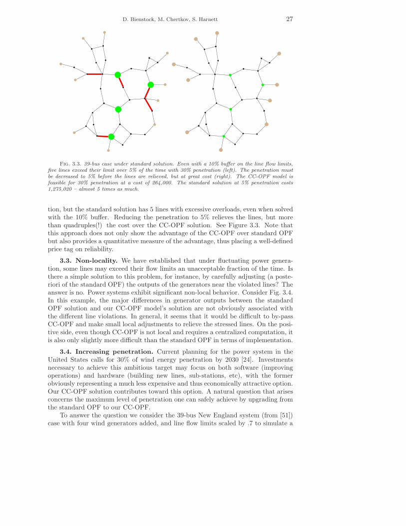
Fig. 3.3. 39-bus case under standard solution. Even with a 10% buffer on the line flow limits,five lines exceed their limit over 5% of the time with 30% penetration (left). The penetration mustbe decreased to 5% before the lines are relieved, but at great cost (right). The CC-OPF model isfeasible for 30% penetration at a cost of 264,000. The standard solution at 5% penetration costs1,275,020 – almost 5 times as much.

tion, but the standard solution has 5 lines with excessive overloads, even when solvedwith the 10% buffer. Reducing the penetration to 5% relieves the lines, but morethan quadruples(!) the cost over the CC-OPF solution. See Figure 3.3. Note thatthis approach does not only show the advantage of the CC-OPF over standard OPFbut also provides a quantitative measure of the advantage, thus placing a well-definedprice tag on reliability.

3.3. Non-locality. We have established that under fluctuating power genera-tion, some lines may exceed their flow limits an unacceptable fraction of the time. Isthere a simple solution to this problem, for instance, by carefully adjusting (a poste-riori of the standard OPF) the outputs of the generators near the violated lines? Theanswer is no. Power systems exhibit significant non-local behavior. Consider Fig. 3.4.In this example, the major differences in generator outputs between the standardOPF solution and our CC-OPF model’s solution are not obviously associated withthe different line violations. In general, it seems that it would be difficult to by-passCC-OPF and make small local adjustments to relieve the stressed lines. On the posi-tive side, even though CC-OPF is not local and requires a centralized computation, itis also only slightly more difficult than the standard OPF in terms of implementation.

3.4. Increasing penetration. Current planning for the power system in theUnited States calls for 30% of wind energy penetration by 2030 [24]. Investmentsnecessary to achieve this ambitious target may focus on both software (improvingoperations) and hardware (building new lines, sub-stations, etc), with the formerobviously representing a much less expensive and thus economically attractive option.Our CC-OPF solution contributes toward this option. A natural question that arisesconcerns the maximum level of penetration one can safely achieve by upgrading fromthe standard OPF to our CC-OPF.

To answer the question we consider the 39-bus New England system (from [51])case with four wind generators added, and line flow limits scaled by .7 to simulate a


Fig. 3.4. 39-bus case. Red lines indicate high probability of flow exceeding the limit underthe standard OPF solution. Generators are shades of blue, with darker shades indicating greaterabsolute difference between the chance-constrained solution and the standard solution.

heavily loaded system. The quadratic cost terms are set to rand(0,1) + .5. We fix thefour wind generator average outputs in a ratio of 5/6/7/8 and standard deviations at30% of the mean. We first solve our model using ǫ = .02 for each line and assumingzero wind power, and then increase total wind output until the optimization problembecomes infeasible. See Figure 3.5. This experiment illustrates that at least forthe model considered, the 30% of wind penetration with rather strict probabilisticguarantees enforced by our CC-OPF may be feasible, but in fact lies rather close tothe dangerous threshold. To push penetration beyond the threshold is impossiblewithout upgrading lines and investing in other (not related to wind farms themselves)hardware.

3.5. Changing locations for wind farms. In this example we consider theeffect of changing locations of wind farms. We take the MATPOWER 30-bus casewith line capacities scaled by .75 and add three wind farms with average power output


Fig. 3.5. 39-bus case with four wind farms (green dots; brown are generators, black are loads).Lines in red are at the maximum of ǫ = .02 chance of exceeding their limit. The three cases shownare left to right .1%, 8%, and 30% average wind penetration. With penetration beyond 30% theproblem becomes infeasible.

Fig. 3.6. 30-bus case with three wind farms. The case on the left supports only up to 10%penetration before becoming infeasible, while the one on the right is feasible for up to 55% penetration.

in a ratio of 2/3/4 and standard deviations at 30% of the average. Two choices oflocations are shown in figure 3.6. The first remains feasible for penetration up to 10%while the second can withstand up to 55% penetration. This experiment shows thatchoosing location of the wind farms is critical for achieving the ambitious goal of highrenewable penetration.

3.6. Reversal of line flows. Here we consider the 9-bus case with two windsources and 25% average penetration and standard deviations set to 30% of the av-erage case and analyze the following two somewhat rare but still admissible windconfigurations: (1) wind source (a) produces its average amount of power and source(b) three standard deviations below average; (2) the reverse of the case (1). Thisresults in a substantial reversal of flow on a particular line shown in Figure 3.7. Thisexample suggests that when evaluating and planning for grids with high-penetrationof renewables one needs to be aware of potentially fast and significant structural re-arrangements of power flows. Flow reversals and other qualitative changes of powerflows, which are extremely rare in the grid of today, will become significantly muchmore frequent (typical) in the grid of tomorrow.


9.716.21

Fig. 3.7. 9-bus case, 25% average penetration from two wind sources. With shifting winds, theflow on the orange line changes direction with a large absolute difference.

3.7. Out-of-sample tests. We now study the performance of the control com-puted using nominal CC-OPF when there are errors in the underlying distribution ofwind power. We consider two types of errors: (1) the true distribution is non-Gaussianbut our Gaussian fit is “close” in an appropriate sense, and (2) the true distributionis Gaussian but with different mean or standard deviation. The experiments in thissection use as data set the BPA grid, which as noted before has 2209 buses and 2866lines, and collected wind data; altogether constituting a realistic test-case.

We first consider the non-Gaussian case, using the following probability distribu-tions, all with fatter tails than Gaussian: (1) Laplace, (2) logistic, (3) Weibull (threedifferent shapes), (4) t location-scale with 2.5 degrees of freedom, (5) Cauchy. For theLaplace and logistic distributions, we simply match the mean and standard deviation.For the Weibull distribution, we consider shape parameters k = 1.2, 2, 4 and choosethe scale parameter to match the standard deviations. We then translate to matchmeans. For the t distribution, we fix 2.5 degrees of freedom and then choose the loca-tion and scale to match mean and standard deviation. For the Cauchy distribution,we set the location parameter to the mean and choose the scale parameter so as tomatch the 95th percentiles.

We use our model and solve under the Gaussian assumption, seeking a solutionwhich results in no line violations for cases within two standard deviations of the mean,i.e. a maximum of about 2.27% chance of exceeding the limit. We then perform MonteCarlo tests drawing from the above distributions to determine the actual rates ofviolation. See Figure 3.8. The worst-performer is the highly-asymmetric (and perhapsunreasonable) Weibull with shape parameter 1.2, which approximately doubles thedesired maximum chance of overload. Somewhat surprisingly, the fat-tailed logisticand Student’s t distributions result in a maximum chance of overload significantlyless than desired, suggesting that our model is too conservative in these cases.

Next we consider the Gaussian case with errors. We solve with nominal valuesfor the mean and standard deviation of wind power. We then consider the rate ofviolation after scaling all means and standard deviations (separately) . While the


Distribution Max. prob. violation

Normal 0.0227Laplace 0.0297logistic 0.0132Weibull, k = 1.2 0.0457Weibull, k = 2 0.0355Weibull, k = 4 0.0216t location-scale, ν = 2.5 0.0165Cauchy 0.0276

Fig. 3.8. Maximum probability of overload for out-of-sample tests. These are a result of MonteCarlo testing with 10,000 samples on the BPA case, solved under the Gaussian assumption anddesired maximum chance of overload at 2.27%.

−0.5 −0.25 0 0.25 0.50

0.1

0.2

0.3

0.4

0.5

Forecast error

Max

pro

b. li

ne o

verlo

ad

mean errorstandard deviation error

Fig. 3.9. BPA case solved with average penetration at 8% and standard deviations set to 30% ofmean. The maximum probability of line overload desired is 2.27%, which is achieved with 0 forecasterror on the graph. Actual wind power means are then scaled according to the x-axis and maximumprobability of line overload is recalculated (blue). The same is then done for standard deviations(green).

solution is sensitive to errors in the mean forecast, the sensitivity is well-behaved.With a desired safety level of ǫ = 2.27% for each line, an error in the mean of 25%results in a maximum 15% chance of exceeding the limit. The solution is quite robustto errors in the standard deviation forecast, with a 25% error resulting in less than6% chance of overload. See Figure 3.9.

3.8. Scalability. As an additional experiment illustrating scalability of the ap-proach we studied the Polish national grid (obtained from MATPOWER as explainedabove) under simulated 20 % renewable penetration spread over 18 wind farms, co-located with the 18 largest generators. This co-location should lessen the risk as-sociated with renewable fluctuation (which should be partially “absorbed” by theco-located generators). Figure 3.10 studies the resulting risk exposure under stan-dard OPF. The chart shows the number of lines that attain several levels of overloadprobability. The situation in the chart is unacceptable: it would lead to frequenttripping of at least four lines.

In contrast, Figure 3.11 shows the performance attained by the chance-constrainedOPF in the same setting as that of Figure 3.10. Notice the drastic reduction inoverload probabilities – the system is stable. Moreover, this is attained with a minorincrease in cost (less than one percent) while the computational time is on the order


of 10 seconds.

1 2 3 40

0.011

0.019

0.029

0.051

0.087

ProbabilityOverload

# of lines

Standard OPF

0.5

0.32

Fig. 3.10. Figure shows number of lines that are overloaded with given probability values insimulation of 2746 bus Polish power grid using standard OPF with 20% wind penetration distributedover 18 wind farms. In particular, two lines are overloaded half of the time, and one line is over-loaded one-third of the time, constituting a situation with unacceptable systemic risk.

1 3 40

ProbabilityOverload

# of lines

0.0017

0.0016

0.0021

0.002

0.0019

0.0018

Chance−constrained OPF

2

0.0024

Fig. 3.11. Same as Figure 3.10, but under chance-constrained OPF. Notice that the largestoverload probability is 200 times smaller than in the case of standard OPF. Moreover, the costincrease is by less than one percent

4. Discussions. This manuscript suggests a new approach to incorporating un-certainty in the standard OPF setting routinely used in the power industry to setgeneration during a time window, or period (typically 15 min to one hour duration).When uncertainty associated with renewable generation is quantified in terms of theprobability distribution of output during the next period, we incorporate it throughchance constraints - probabilistic conditions which require that any line of the sys-tem will not be overloaded for all but a small fraction of time (at most one minuteper hour, for example). Additionally, the modeling accounts for local frequency re-


sponse of controllable generators to renewable changes. The key technical result ofthis manuscript is that the resulting optimization problem, CC-OPF, can be stated asa convex, deterministic optimization problem. This result also relies on plausible as-sumptions regarding the exogenous uncertainty and linearity of the underlying powerflow approximations/equations. In fact, our CC-OPF is a convex (conic) optimizationproblem, which we solve very efficiently, even on realistic large-scale instances, usinga sequential linear cutting plane algorithm.

This efficient CC-OPF algorithm becomes an instrument of our (numerical) ex-periments which were performed on a number of standard (and nonstandard) powergrid data sets. Our experimental results are summarized as follows:

• We observe that CC-OPF delivers feasible results where standard OPF, runfor the average forecast, would fail in the sense that many lines would beoverloaded an unacceptably large portion of time.

• Not only is CC-OPF safer than standard OPF, but it also results in cheaperoperation. This is demonstrated by considering the optimal cost of CC-OPFunder sufficiently high wind penetration solution (where standard OPF wouldfail) and the low penetration solution (corresponding to the highest possiblepenetration where standard OPF would not fail).

• We discover that solutions produced by CC-OPF deviate significantly fromwhat amounts to a the naive adjustment of the standard OPF obtained bycorrecting dispatch just at those generators which are close to overloadedlines.

• We test the level of wind penetration which can be tolerated without upgrad-ing lines. This experiment illustrates that, at least for the model tested, the30% of wind penetration with rather strict probabilistic guarantees enforcedby our CC-OPF may be feasible; but much lower wind penetration remainsfeasible under the standard approach.

• We experiment with location of wind farms and discover strong sensitivity ofthe maximum level of penetration on the choice of location - optimal choiceof wind farm location is critical for achieving the ambitious goal of highrenewable penetration.

• Analyzing fluctuations of line flows within CC-OPF solution admissible underhigh wind penetration, we discover that these fluctuations may be significant,in particular resulting in reversal of power flows over some of the lines. Thisobservation suggests that flow reversals and other qualitative changes of powerflows, which are extremely rare in the grid of today, will become significantlymuch more frequent (typical) in the grid of tomorrow.

• We studied an out-of-sample test consisted in applying CC-OPF (modelingexogenous fluctuations as Gaussian) to other distributions. Overall these testssuggest that with a proper calibration of the effective Gaussian distributionour CC-OPF delivers a rather good performance. One finds that the worstCC-OPF performance is observed for the most asymmetric distributions.

• We also presented a computationally sound data-robust version of the CC-OPF where the parameters for the Gaussian distributions are assumed un-known, but lying in a window. This allows for parameter mis-estimation, formodel error, and it is also suggests a way to deal in a tractable way withnon-Gaussian fluctuations.

The nature of the problem discussed in the manuscript – principal design of anew paradigm for computationally efficient generation re-dispatch that accounts for


wind fluctuations – inevitably required incorporation of a number of assumptions andapproximations. In particular, we made simplifying assumptions about static forecastsand general validity of power flow linearization. We have also focused solely on failuresassociated with line congestion ignoring other possible difficulties, for example thoseassociated with loss of synchronicity and voltage variations. However, we would liketo emphasize that all of these assumptions made (admittedly natural for a first attackon the problem) also allow generalization within the approach just sketched:

• Accounting for time evolving forecast/loads/etc. Wind forecast, expressed interms of the mean and standard deviation at the wind farm sites, changeson the scales comparable to duration of the generation re-dispatch interval.Loads may also change at these time scales. When the slowly evolving, butstill not constant, wind and load forecasts are available we may keep thequasi-static power flow description and incorporate this slow evolution intime into the chance constrained scheme. These changes will simply result ingeneralizing the conic formulation (2.29)-(2.37) by splitting what used to bea single time interval into sub-intervals and allowing the regular generation tobe re-dispatched and parallel coefficients to be adjusted more often. Rampingrate constraints on the controllable generation may naturally be accountedin the temporal optimization scheme as well.

• Accounting for nonlinearity in power flows. Evolution of the base case inval-idates the linearization (DC-style) hypothesis. However, if variations aroundone base case becomes significant one may simply adjust the linearization pro-cedure doing it not once (as in the case considered in the manuscript) but asoften as needed. Slow adjustment of the base case may also be included intothe dynamical procedure mentioned one item above. Additionally, some inter-esting new methodologies for handling nonlinearities have recently emerged,see [36].

• Accounting for synchronization bounds. Loss of synchronicity and resultingdisintegration of the grid is probably the most acute contingency which canpossibly take place in a power system. The prediction of those conditionsunder which the power grid will lose synchronicity is a difficult nonlinear anddynamic problem. However, as shown recently in [23], one can formulate anaccurate linear and static necessary condition for the loss of synchronicity.A chance-constrained version of the linear synchronization conditions can beincorporated seamlessly in our CC-OPF framework.

Finally, we see many opportunities in utilizing the CC-OPF (possibly modified) asan elementary unit or an integral part of even more complex problems, such as com-bined unit commitment (scheduling large power plants normally days, weeks or evenmonths ahead) [47] with CC-OPF, planning grid expansion [4] while accounting forcost operation under uncertainty, or incorporating CC-OPF in mitigating emergencyof possible cascades of outages [17, 40, 44, 43, 9, 10, 25, 6]. In this context, it wouldbe advantageous to speed up our already very efficient CC-OPF even further. See,for example, [11], [8]. A different methodology, relying on distributed algorithms, canbe found in [34].

5. Acknowledgments. We are thankful to S. Backhaus and R. Bent for theircomments, and to K. Dvijotham for help with BPA data. The work at LANL wascarried out under the auspices of the National Nuclear Security Administration ofthe U.S. Department of Energy at Los Alamos National Laboratory under ContractNo. DE-AC52-06NA25396. MC and SH also acknowledge partial support of the


DTRA Basic Research grant BRCALL08-Per3-D-2-0022. DB and SH were partiallysupported by DOE award DE-SC0002676.

REFERENCES

[1] Robust portfolio selection problems.[2] S. Baghsorkhi and I. Hiskens, Analysis tools for assessing the impact of wind power on weak

grids, SysCon, (2012), pp. 1 –8.[3] R. Ben-Tal and A. Nemirovski, Robust solutions of linear programming problems contami-

nated with uncertain data, Mathematical Programming, 88 (2000), pp. 411–424.[4] R. Bent, G. Toole, and A. Berscheid, Transmission network expansion planning with com-

plex power flow models, Power Systems, IEEE Transactions on, 27 (2012), pp. 904 –912.[5] A. Bergen and V. Vittal, Power System Analysis, Prentice Hall. Inc, 2000.[6] A. Bernstein, D. Hay, M. Uzunoglu, and G. Zussman, Power grid vulnerability to geo-

graphically correlated failures - analysis and control implications. http://arxiv.org/abs/1206.1099, 2012.

[7] D. Bertsimas and M. Sim, Price of robustness, Operations Research, 52 (2004), pp. 35–53.[8] D. Bienstock, Potential Function Methods for Approximately Solving Linear Programming

Problems, Theory and Practice, Kluwer, 2002.[9] D. Bienstock, Adaptive online control of cascading blackouts, Proc. 2011 IEEE Power and

Energy Society General Meeting, (2011), pp. 1–8.[10] , Optimal control of cascading power grid failures, Proc 2011 CDC-ECC, (2011), pp. 2166

–2173.[11] D. Bienstock and G. Iyengar, Faster approximation algorithms for covering and packing

problems, SIAM Journal on Computing, 35 (2006), pp. 825–854.[12] H. Bludszuweit, J. Dominguez-Navarro, and A. Llombart, Statistical analysis of wind

power forecast error, Power Systems, IEEE Transactions on, 23 (2008), pp. 983 –991.[13] S. Boyd and L. Vandenberghe, Convex Optimization, Cambridge University Press, 2004.[14] BPA-WIND, Wind generation & total load in the bpa balancing authority. http://

transmission.bpa.gov/business/operations/wind/, 2012.[15] CAISO, Integration of renewable resources: Transmission and operating issues and rec-

ommendations for integrating renewable resources on the california iso-controlled grid.http://www.caiso.com/1ca5/1ca5a7a026270.pdf, 2007.

[16] A. Charnes, W. Cooper, and G. Symonds, Cost horizons and certainty equivalents: anapproach to stochastic programming of heating oil, Management Science, 4 (1958), pp. 235–263.

[17] J. Chen, J. Thorp, and I. Dobson, Cascading dynamics and mitigation assessment in powersystem disturbances via a hidden failure model, International Journal of Electrical Power;Energy Systems, 27 (2005), pp. 318 – 326.

[18] M. Chertkov, F. Pan, and M. Stepanov, Predicting failures in power grids: The case ofstatic overloads, IEEE Transactions on Smart Grids, 2 (2010), p. 150.

[19] M. Chertkov, M. Stepanov, F. Pan, and R. Baldick, Exact and efficient algorithm todiscover extreme stochastic events in wind generation over transmission power grids, CDC-ECC, (2011), pp. 2174 –2180.

[20] CIGRE, Technical brochure on grid integration of wind generation, International Conferenceon Large High Voltage Electric Systems, (2009).

[21] CPLEX, ILOG CPLEX Optimizer. http://www-01.ibm.com/software/integration/

optimization/cplex-optimizer/, 2012.[22] DENA, Energy management planning for the integration of wind energy into the grid in ger-

many, onshore and offshore by 2020, (2005).[23] F. Dorfler, M. Chertkov, and F. Bullo, Synchronization in Complex Oscillator Networks

and Smart Grids, http://arxiv.org/abs/1208.0045, (2012).[24] EERE, 20% of wind energy by 2030: Increasing wind energy’s contribution to us electricity

supply, Department of Energy (DOE), DOE/GO-102008-2567 (2008).[25] M. Eppstein and P. Hines, A ”random chemistry” algorithm for identifying collections of

multiple contingencies that initiate cascading failure, Power Systems, IEEE Transactionson, 27 (2012), pp. 1698–1705.

[26] E. Erdogan and G. Iyengar, Ambiguous chance constrained problems and robust optimiza-tion, Mathematical Programming, 107 (2007), pp. 37–61.

[27] U.-C. P. S. O. T. Force, Report on the august 14, 2003 blackout in the united states andcanada: Causes and recommendations. https://reports.energy.gov, (2004).


[28] D. Goldfarb and F. Alizadeh, Second-order cone programming, Mathematical Programming,95 (2003), pp. 3–51.

[29] G. Gonzalez and et al., Experience integrating and operating wind power in the peninsularspanish power system. point of view of the transmission system operator and a wind powerproducer, CIGRE, (2006).

[30] M. Grotschel, L. Lovasz, and A. Schrijver, Geometric Algorithms and CombinatorialOptimization, Springer-Verlag, 1998.

[31] GUROBI, Optimizer. http://www.gurobi.com/, 2012.[32] B.-M. Hodge and M. Milligan, Wind power forecasting error distributionsover multiple

timescales, Detroit Power Engineering Society Meeting, (2011), pp. 1–8.[33] M. Huneault, A survey of the optimal power flow literature, Power Systems, IEEE Transac-

tions, (1991).[34] M. Kraning, E. Chu, J. Lavaei, and S. Boyd, Message passing for dynamic network energy

management. http://www.stanford.edu/~boyd/papers/decen_dyn_opt.html, 2012.[35] P. Kundur, Power System Stability and Control, McGraw-Hill, New York, NY, USA, 1994.[36] J. Lavaei and S. Low, Zero duality gap in optimal power flow problem, IEEE Transactions on

Power Systems, 27 (2012), pp. 92–107.[37] Y. Makarov, C. Loutan, J. Ma, and P. de Mello, Operational impacts of wind generation

on california power systems, Power Systems, IEEE Transactions on, 24 (2009), pp. 1039–1050.

[38] L. Miller and H. Wagner, Chance-constrained programming with joint constraints, Opera-tions Research, 13 (1965), pp. 930–945.

[39] MOSEK, Optimizer. http://www.mosek.com/, 2012.[40] D. Nedic, I. Dobson, D. Kirschen, B. Carreras, and V. E. Lynch, Criticality in a cascad-

ing failure blackout model, International Journal of Electrical Power; Energy Systems, 28(2006), pp. 627 – 633.

[41] A. Nemirovski and A. Shapiro, Convex approximations of chance constrained programs,SIAM Journal on Optimization, 17 (2006), pp. 969–996.

[42] U. Ozturk and M. Mazumdar, A solution to the stochastic unit commitment problem usingchance constrained programming, Power Systems, IEEE, 19 (2004), pp. 1589–1598.

[43] R. Pfitzner, K. Turitsyn, and M. Chertkov, Controlled Tripping of Overheated LinesMitigates Power Outages, arxiv:1104.4558, (2011).

[44] R. Pfitzner, K. Turitsyn, and M. Chertkov, Statistical classification of cascading failuresin power grids, in Power and Energy Society General Meeting, 2011 IEEE, july 2011, pp. 1–8.

[45] A. Prekopa, On probabilistic constrained programming, Proc. Princeton Symposium on Math.Programming, (1970), pp. 113–138.

[46] G. Wang, M. Negrete-Pincetic, A. Kowli, E. Shafieepoorfard, S. Meyn, and

U. Shanbhag, Dynamic competitive equilibria in electricity markets, in Control and Op-timization Theory for Electric Smart Grids, A. Chakrabortty and M. Illic, eds., Springer,2011.

[47] J. Wang, M. Shahidehpour, and Z. Li, Security-constrained unit commitment with volatilewind power generation, Power Systems, IEEE Transactions on, 23 (2008), pp. 1319 –1327.

[48] M. Wyld, Wind energy bumps into power grid limits, New York Times, (2008/08/27).[49] H. Zhang, Chance Constrained Programming for Optimal Power Flow Under Uncertainty,

Power Systems, IEEE Transactions on, 26 (2011), pp. 2417–2424.[50] S. Zhang, Y. Song, Z. Hu, and L. Yao, Robust optimization method based on scenario analysis

for unit commitment considering wind uncertainties, in Power and Energy Society GeneralMeeting, 2011 IEEE, july 2011, pp. 1 –7.

[51] R. Zimmerman, C. Murillo-Sanchez, and R. Thomas, Matpower: Steady-state operations,planning, and analysis tools for power systems research and education, Power Systems,IEEE Transactions on, 26 (2011), pp. 12 –19.

chance constrained optimal power flow: …dano/papers/cc-opf3.pdfchance constrained optimal power...

Documents