chance constrained optimal power flow: …dano/papers/cc-opf4.pdf · chance constrained optimal...
TRANSCRIPT
CHANCE CONSTRAINED OPTIMAL POWER FLOW:RISK-AWARE NETWORK CONTROL UNDER UNCERTAINTY
DANIEL BIENSTOCK ∗, MICHAEL CHERTKOV † , AND SEAN HARNETT ‡
Abstract. When uncontrollable resources fluctuate, Optimum Power Flow (OPF), routinelyused by the electric power industry to re-dispatch hourly controllable generation (coal, gas and hy-dro plants) over control areas of transmission networks, can result in grid instability, and, potentially,cascading outages. This risk arises because OPF dispatch is computed without awareness of majoruncertainty, in particular fluctuations in renewable output. As a result, grid operation under OPFwith renewable variability can lead to frequent conditions where power line flow ratings are signifi-cantly exceeded. Such a condition, which is borne by simulations of real grids, would likely resultingin automatic line tripping to protect lines from thermal stress, a risky and undesirable outcomewhich compromises stability. Smart grid goals include a commitment to large penetration of highlyfluctuating renewables, thus calling to reconsider current practices, in particular the use of standardOPF. Our Chance Constrained (CC) OPF corrects the problem and mitigates dangerous renewablefluctuations with minimal changes in the current operational procedure. Assuming availability ofa reliable wind forecast parameterizing the distribution function of the uncertain generation, ourCC-OPF satisfies all the constraints with high probability while simultaneously minimizing the costof economic re-dispatch. CC-OPF allows efficient implementation, e.g. solving a typical instanceover the 2746-bus Polish network in 20 seconds on a standard laptop.
Key words. Optimization, Power Flows, Uncertainty, Wind Farms, Networks
The power grid, one of the greatest engineering achievements of the 20th century,delivers social development and resulting political stability of billions of people aroundthe globe through control sophistication and careful long-term planning, with onlyvery rare disruptions.
However, the grid is under growing stress and the premise of secure electricalpower may become less certain. Despite massive investments large-scale power out-ages occur unpredictably and with increasing frequency. Automatic grid control andregulations achieve robustness of operation as under normal fluctuations, in particu-lar under approximately predicted inter-day demand trends, or even single points offailure, such as the failure of a generator or tripping of a single line. However, larger,unexpected events can prove difficult to overcome. A case could be made that powergrids could have greater reliance on physical models and on data-driven algorithms.Despite remarkable sophistication, in particular highly efficient distributed frequencyand voltage controls, very often, should an unusual condition arise, current grid oper-ation relies on human input. Additionally, only some real-time data is actually usedby the grid to respond to evolving conditions.
A benefit of a cost-effective migration toward a more algorithmic-driven gridconcerns the effective integration of renewables. This issue is critical because large-scale introduction of renewables brings with it the risk of large, random variability –a condition that the current grid was not developed to accommodate.
This issue becomes clear when we considering so-called Optimal Power Flow(OPF) or economic dispatch, used to set generator output in typically 15-minute
∗Department of Industrial Engineering and Operations Research and Department of AppliedPhysics and Applied Mathematics, Columbia University, 500 West 120th St. New York, NY 10027USA ([email protected]).
†Theoretical Division and Center for Nonlinear Studies, Los Alamos National Laboratory, NM87545 USA ([email protected]).
‡Department of Applied Physics and Applied Mathematics, Columbia University, 500 West 120thSt. New York, NY 10027 USA and Center for Nonlinear Studies, Los Alamos National Laboratory,NM 87545 USA.
1
2 Chance Constrained Optimal Power Flow
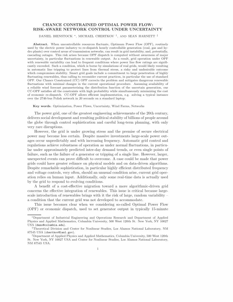
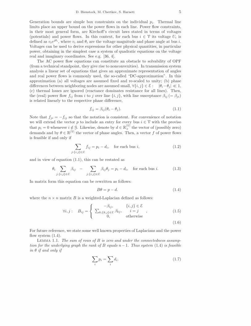
Fig. 0.1. Bonneville Power Administration [13] shown in outline under 9% wind penetration,where green dots mark actual wind farms. We set standard deviation to be 0.3 of the mean for eachwind source. Our CC-OPF (with 1% of overload set as allowable) resolved the case successfully (nooverloads) and was computed in seconds, while the standard OPF showed 8 overloaded lines, allmarked in color. Lines shown orange are at 4% chance of overload. There are two dark red lineswhich are at 50% of the overload while other (dark orange) lines show values of overload around10%.
windows (more frequently in some cases). OPF sets generator outputs so as to meetdemand at minimum cost, under operating limitations of generators and transmissionlines. Estimates of the typical loads for the upcoming time window are employed inthis computation. This scheme can fail, dramatically, when renewables are part of thegeneration mix and (exogenous) fluctuations in renewable output become large. By“failure” we mean, in particular, not accounting for instances where a combination ofgenerator and renewable outputs conspire to produce power flows that significantlyexceed power line ratings. When a line’s rating is exceeded, the line becomes morelikely to trip (be taken out of service) compromising the integrity and stability ofthe grid. To correct for this scenario an additional scheme, based on direct line flowmeasurements and requiring a human operator in the loop, is employed as a part ofthe current operational routine – after receiving a warning, the operator may initiatean emergency action, possibly disconnecting the overheated line.
Under the forthcoming high wind power penetration, significantly more frequentline overloads are likely, making the current operational paradigm clearly unsustain-
D. Bienstock, M. Chertkov, S. Harnett 3
able. If several key lines become tripped a grid would very likely become unstable andpossibly experience a cascading failure, with large losses in serviced demand. This isnot an idle assumption, since firm commitments to major renewable penetration arein place throughout the world. For example, 20% renewable penetration by 2030 is adecree in the U.S. [24], and similar plans are to be implemented in Europe, see e.g.discussions in [19, 21, 29]. At the same time, operational margins (between typicalpower flows and line ratings) are decreasing and expected to decrease in part dueto deregulation and difficulties in expanding transmission capacity [19]. A possiblefailure scenario is illustrated in Fig. 0.1 using as example the U.S. Pacific Northwestregional grid data (2866 lines, 2209 buses, 176 generators and 18 wind sources), wherelines highlighted in red are jeopardized (flow becomes too high) with unacceptablyhigh probability by fluctuating wind resources positioned along the Columbia riverbasin (green dots marking existing wind farms).
We propose a solution that requires, as the only additional investment, accuratewind forecasts; but no change in machinery or significant operational procedures.Instead, we propose to mitigate risk using an efficient algorithmic modification of theOPF approach. In computational experiments our algorithm solves realistic exampleswith thousands of buses and lines (such as the U.S. Pacific Northwest case) in a matterof seconds, and is thus only slightly slower than standard economic dispatch methodseven on large-scale case.
It is natural to assess the risk of an event such as a line overload in terms of prob-abilities, because of the non-deterministic behavior of e.g. wind; thus our proposedapproach relies on mathematical optimization and risk analysis. In a system understochastic risk, an extremely large variety of events that could pose danger mightemerge. Recent works [17, 18, 1] suggest that focusing on instantons, or most-likely(dangerous) events, provides a practicable route to risk control and assessment. How-ever, there may be far too many comparably probable instantons, and furthermore,we need a computationally efficient methodology that not only identifies dangerous,relatively probable events, but also mitigates them.
This paper suggests a new approach that searches for the most probable real-izations of line overloads under renewable generation, and corrects such situationsthrough control actions, simultaneously and efficiently in one step. Our approachrelies on “Chance-Constrained” (CC) optimization [42]. Broadly speaking, CC op-timization problems are optimization problems under uncertainty, with constraintsstating that the probability of a certain random event is kept smaller than a targetvalue.
We model each bus that houses a power source subject to randomness to include arandom power injection. Our reformulation of standard OPF so minimizes the averagecost of generation over the random power injections, while specifying a mechanism bywhich (standard, i.e. controllable) generators compensate in real-time for renewablepower fluctuations so as to guarantee low probability that any line will exceed itsrating. This last constraint is naturally formulated as a chance constraint – we termour approach Chance-Constrained OPF, or CC-OPF.
This paper is organized as follows. In Section 1 we motivate and present thevarious mathematical models used to describe how the grid operates, as well as ourproposed methodology. We explain how to solve the models in Section 2. We thenpresent, in Section 3 a number of examples to demonstrate the speed and usefulnessof our approach. Section 4 summarizes the results and discusses the path forward.
1. Formulating Chance-Constrained Optimum Power Flow Models.
4 Chance Constrained Optimal Power Flow
1.1. Transmission Grids: Controls and Limits. In this paper we considertransmission grids which operate at high voltages so as to convey power economically,with minimal losses, over large distances. In contrast distribution systems are typicallyresidential, lower voltage grids used to provide power to individual consumers. Fromthe point of view of wind-power generation, smooth operation of transmission systemsis key since reliable wind sources are frequently located far away from consumption.
Transmission systems balance consumption/load and generation using a complexstrategy that spans three different time scales (see e.g. [4]). At any point in time, gen-erators produce power at a previously computed base level; power is generated (andtransmitted) in the Alternating Current (AC) form. An essential stability ingredientsis that all generators operate at a common frequency (e.g. 60 Hz in North America).In real time, changes in loads are registered at generators through (opposing) changesin frequency. Consider the case of a sudden load increase. In that case generatorfrequency will start to drop. The so-called primary frequency control, normally im-plemented on some gas and hydro plants, will react so as to stop frequency drift, byhaving each responding generator convey more power to the system, proportionallyto the frequency change. This reaction is swift and local, leading to stabilizationof frequency across the system, however not necessarily at the nominal 60Hz value.The task of the secondary, or Automatic Generation Control (AGC), is to undertakethe adjustment of generation levels to return frequency to the nominal value.1 TheOPF algorithm typically runs as frequently as every 15 minutes providing informationfor AGC, which ultimately undertakes the adjustment of generation levels to achieveoptimal (or close to optimal) control. The OPF time-window thus represents theshortest time scale where actual off-line and network wide optimal computations areemployed.
1.2. OPF – Standard Generation Dispatch. As discussed above OPF [33,36, 4] is used to reset generator output levels over a control area of the transmissiongrid (for example over the Bonneville Power Administration (BPA) grid shown inFig. 0.1). In order to describe OPF we will employ power engineering terms such as“bus” to refer to a graph-theoretic vertex and “line” to refer to an edge. The set ofall buses will be denoted by V, the set of lines, E and the set of buses that house gen-erators, G. We let n = |V|. A line joining buses i and j is denoted by i, j indicatingan unordered pair. We assume that the underlying graph is connected, without lossof generality.
The generic OPF problem can be stated as follows:• The goal is to determine the vector p ∈ R
G, where for i ∈ G, pi is the outputof generator i, so as to minimize an objective function c(p). This function is,usually, a convex, separable quadratic function of p:
c(p) =∑
i∈G
ci(pi),
where each ci is convex quadratic.• The problem is endowed by three types of constraints: power flow, line limit
and generation bound constraints.
1AGC is based on SCADA communications, which is receiving an updated signal every 4s or so,however, the actual control action is computed based on integration of the SCADA communicatedsignal over a longer window of several minutes.
D. Bienstock, M. Chertkov, S. Harnett 5
Generation bounds are simple box constraints on the individual pi. Thermal linelimits place an upper bound on the power flows in each line. Power flow constraints,in their most general form, are Kirchoff’s circuit laws stated in terms of voltages(potentials) and power flows. In this context, for each bus i ∈ V its voltage Ui isdefined as vie
jθi , where vi and θi are the voltage magnitude and phase angle at bus i.Voltages can be used to derive expressions for other physical quantities, in particularpower, obtaining in the simplest case a system of quadratic equations on the voltagereal and imaginary coordinates. See e.g. [36, 4].
The AC power flow equations can constitute an obstacle to solvability of OPF(from a technical standpoint, they give rise to nonconvexities). In transmission systemanalysis a linear set of equations that gives an approximate representation of anglesand real power flows is commonly used, the so-called “DC-approximation”. In thisapproximation (a) all voltages are assumed fixed and re-scaled to unity; (b) phasedifferences between neighboring nodes are assumed small, ∀i, j ∈ E : |θi−θj| ≪ 1,(c) thermal losses are ignored (reactance dominates resistance for all lines). Then,the (real) power flow fij from i to j over line i, j, with line susceptance βij (= βji)is related linearly to the respective phase difference,
fij = βij(θi − θj). (1.1)
Note that fji = −fij so that the notation is consistent. For convenience of notationwe will extend the vector p to include an entry for every bus i ∈ V with the proviso
that pi = 0 whenever i /∈ G. Likewise, denote by d ∈ R|V|+ the vector of (possibly zero)
demands and by θ ∈ R|V| the vector of phase angles. Then, a vector f of power flows
is feasible if and only if∑
j:i,j∈E
fij = pi − di, for each bus i, (1.2)
and in view of equation (1.1), this can be restated as
θi
∑
j:i,j∈E
βij −∑
j:i,j∈E
βijθj = pi − di, for each bus i. (1.3)
In matrix form this equation can be rewritten as follows:
Bθ = p − d. (1.4)
where the n × n matrix B is a weighted-Laplacian defined as follows:
∀i, j : Bij =
−βij , i, j ∈ E∑
k;k,j∈Eβkj , i = j
0, otherwise, (1.5)
(1.6)
For future reference, we state some well known properties of Laplacians and the powerflow system (1.4).
Lemma 1.1. The sum of rows of B is zero and under the connectedness assump-tion for the underlying graph the rank of B equals n−1. Thus system (1.4) is feasiblein θ if and only if
∑
i
pi =∑
i
di. (1.7)
6 Chance Constrained Optimal Power Flow
In other words: under the DC model the power flow Eqs. (1.4) are feasible preciselywhen total generation equals total demand. Moreover, if Eqs. (1.4) are feasible, thenfor any index 1 ≤ j ≤ n there is a solution with θj = 0.
In summary, the standard DC-formulation OPF problem can be stated as thefollowing constrained optimization problem:
OPF: minp,θ
c(p), s.t. (1.8)
Bθ = p − d, (1.9)
∀i ∈ G : pmini ≤ pi ≤ pmax
i , (1.10)
∀i, j ∈ E : |βij(θi − θj)| ≤ fmaxij , (1.11)
Note that the pmini , pmax
i quantities can be used to enforce the convention pi = 0 foreach i /∈ G; if i ∈ G then pmin
i , pmaxi are lower and upper generation bounds which
are generator-specific. Constraint (1.11) is the line limit constraint for i, j; fmaxij
represents the line limit (typically a thermal limit), which is assumed to be strictlyenforced. This conservative condition will be relaxed in the sequel.
Problem (1.8) is a convex quadratic program, easily solved using modern opti-mization tools. The vector d of demands is fixed in this problem and is obtainedthrough estimation. In practice, however, demand will fluctuate around d; gener-ators then respond by adjusting their output (from the OPF-computed quantities)proportionally to the overall fluctuation as discussed above. This scheme works wellin current practice, as demands do not substantially fluctuate on the time scale forwhich OPF applies.
1.3. Chance constrained OPF: motivation. To motivate our approach weoutline how generator output is modulated, in real time, in response to demand fluc-tuations. Suppose we have computed, using OPF, the output pi for each generator iassuming constant demands d. Let d(t) be the vector of real-time demands at time t.Then so-called “frequency control”, or more properly, primary and secondary controlsin combination will achieve (altogether, on the scale of minutes) the following outputsto quantities pi(t)
pi(t) = pi − ρi
∑
j
(dj − dj(t)) for each i ∈ G. (1.12)
In this equation, the quantities ρi ≥ 0 are fixed and satisfy
∑
i
ρi = 1.
Thus, from (1.12) we obtain
∑
i
pi(t) =∑
i
pi −∑
j
(dj − dj(t)) =∑
j
dj(t),
from Eq. (1.7), in other words, demands are met. The quantities ρi ≥ 0 are generatordependent but essentially chosen far in advance and without regard to short-termdemand forecasts.
Thus, in effect, generator outputs are set in hierarchical fashion – using OPF tocompute a base level, with real-time adjustments as per (1.12) which is furthermore
D. Bienstock, M. Chertkov, S. Harnett 7
risk-unaware. This scheme has worked in the past because of the slow time scales ofchange in uncontrolled resources (mainly loads). That is to say, frequency control andload changes are well-separated. A large error in the forecast or an under-estimationof possible d for the next –e.g., fifteen minute– period may lead to an operationalproblem (see e.g. the discussions in [14, 38]) because even though the vector p(t) is
sufficient to meet average demands, the θ(t) computed from
Bθ(t) = p(t) − d(t)
may give rise to real-time power flows
fij(t).= βij [θi(t) − θj(t)]
that violate constraints (1.11). Even the generator constraints (1.10) may fail to hold.This has not been considered a handicap simply because any resulting line trips arerare, primarily because the deviations di(t) − di will be small in the time scale ofinterest. In effect, the risk-unaware approach that assumes constant demands hasworked well.
This perspective changes when renewable power sources such as wind are incor-porated. We assume that a subset W of the buses holds uncertain power sources(wind farms); for each j ∈ W, write the amount of power generated by source j attime t as µj + ωj(t), where µj is the forecast output of farm j in the time period ofinterest. For ease of exposition, we will assume in what follows that G refers to theset of buses holding controllable generators, i.e. G ∩ W = ∅. Renewable generationcan be incorporated into the OPF formulation (1.8)-(1.11) by simply setting pi = µi
for each i ∈ W. Assuming constant demands but fluctuating renewable generation,the application of the frequency control yields the following analogue to (1.12):
pi(t) = pi − ρi
∑
j∈W
ωj(t) for each i ∈ G, (1.13)
e.g. if∑
j∈Wωj(t) > 0, that is to say, there is a net increase in wind output, then
(controllable) generator output will proportionally decrease.Eq. (1.13) describes how generation will adjust to wind changes, under current
power engineering practice. The hazard embodied in this relationship is that the quan-tities ωj(t) can be large resulting in stochastic changes in power flows, significantenough to overload power lines. The risk of such overloads can be expected to increase(see [19]); this is due to a projected increase of renewable penetration in the future,accompanied by the decreasing gap between normal operation and limits set by linecapacities. Lowering of the thermal limits (the fmax
ij quantities in Eqs. (1.11)) cansucceed in deterministically preventing overloads, but it also forces excessively conser-vative choices of the generation re-dispatch, potentially causing extreme volatility ofthe electricity markets. See e.g. the discussion in [50] on abnormal price fluctuationsin markets that are heavily reliant on renewables.
1.4. Using chance constraints. Power lines do not fail (i.e., trip) instantlywhen their flow thermal limits are exceeded. A line carrying flow that exceeds theline’s thermal limit will gradually heat up and possibly sag, and through a variety ofprocesses (such as a contact), may then trip. The precise process is extremely difficultto calibrate.2 Additionally, the rate at which a line overheats depends on its overload
2We refer the reader to [22] for discussions of line tripping during the 2003 Northeast U.S.-Canadacascading failure.
8 Chance Constrained Optimal Power Flow
which may dynamically change (or even temporarily disappear) as flows adjust due toexternal factors; in our case fluctuations in renewable outputs. What can be statedwith certainty is that the longer a line stays overheated, the higher the probabilitythat it will trip – to put it differently, if a line remains overheated over a durationpossibly measured in minutes, it will trip.
Even though an exact representation of line tripping seems difficult, we can how-ever state a practicable alternative. Ideally, we would use a constraint of the form“for each line, the fraction of the time that it exceeds its limit within a certain timewindow is small”. Direct implementation of this constraint would require resolvingdynamics of the grid over the generator dispatch time window of interest. Instead wepropose the following static proxy of this ideal model, a chance constraint: we willrequire that the probability that a given line exceeds its limit is small.
To formalize this notion, we assume:
W.1. For each i ∈ W, the (stochastic) amount of power generated by source i is ofthe form µi + ωi, where
W.2. µi is constant, assumed known from the forecast, and ωi is a zero meanindependent random variable with known standard deviation σi.
Here and in what follows, we use bold face to indicate uncertain quantities. Let fij
be the flow on a given line i, j, and let 0 < ǫij be small. The chance constraint forline i, j, is:
P (fij > fmaxij ) < ǫij and P (fij < −fmax
ij ) < ǫij ∀ i, j. (1.14)
One could alternatively use
P (|fij | > fmaxij ) < ǫij ∀ i, j, (1.15)
which is more conservative than (1.14). If (1.15) holds then so does (1.14), and if thelatter holds then P (|fij | > fmax
ij ) < 2ǫij . However, (1.14) proves more tractable, andmoreover we are interested in the regime where ǫij is fairly small; thus we estimatethat there is small practical difference between the two constraints; this will be verifiedby our numerical experiments. Likewise, for a generator g we will require that
P (pg > pmaxg ) < ǫg and P (pg < pmin
g ) < ǫg. (1.16)
The parameter ǫg will be chosen extremely small, so that for all practical purposes allgenerator outputs will be guaranteed to stay within respective bounds.
Chance constraints [46], [15], [39] are but one possible methodology for handlinguncertain data in optimization. Broadly speaking, this methodology fits within thegeneral field of stochastic optimization. Constraint (1.14) can be viewed as a “value-at-risk” statement; the closely-related “conditional value at risk” concept provides a(convex) alternative, which roughly stated constrains the expected overload of a lineto remain small, conditional on there being an overload (see [42] for definitions anddetails).
One alternative model would insist on imposing the (much stronger) constraint
P (∃ line i, j s.t. |fij | > fmaxij ) < ǫ, (1.17)
where 0 < ǫ < 1. Nemirovski and Shapiro [42] develop a general framework fordeveloping, under appropriate assumptions, a convex optimization problem with an

D. Bienstock, M. Chertkov, S. Harnett 9
approximate version of constraint (1.17), using methodology inspired by the theoryLarge Deviations.
Reference [52] considers the standard OPF problem under stochastic demands,using chance constraints to guarantee high probability that the system operates withinacceptable bounds. The problem is tackled using a simulation-based local optimiza-tion system; with experiments using a 5-bus and a 30-bus example.
Another related study [49] describes a scenario-based system for reserve schedul-ing with fluctuating wind generation, using chance constraints to limit line or gener-ator overloads. This optimization is tackled via transformation to a convex problemplus a heuristic scheme, with no convergence to global optimum of the nonlinearproblem guaranteed.
Chance constrained optimization has also been discussed recently in relation tothe Unit Commitment problem, which concerns discrete-time planning for operationof large generation units on the scale of hours-to-months, so as to account for thelong-term wind-farm generation uncertainty [43, 51, 53].
1.5. Uncertain power sources. In our model we assume independence of windpower fluctuations at different sites; this is justified by the fact that the wind farmsare sufficiently far away from each other. For the typical OPF time span of 15 minand typical wind speed of 10m/s, fluctuations of wind at the farms more than 10kmapart are not correlated.
We make additional simplifying assumptions that are approximately consistentwith our general physics understanding of fluctuations in atmospheric turbulence;in particular we assume Gaussianity of ωi.
3 We will also assume that only a stan-dard weather forecast (coarse-grained on minutes and kilometers) is available, and nosystematic spillage of wind in its transformation to power is applied4.
Additionally, under the Gaussian assumption, chance constraint (1.14) can becaptured using an optimization framework that proves particularly efficient. We willalso consider a data-robust version of our chance-constrained problem where the pa-rameters for the Gaussian distributions are not precisely known. This allows both forparameter mis-estimation and for model error, that is to say the implicit approxima-tion of non-Gaussian distributions with Gaussians; our approach, detailed in Section2.4, remains computationally sound in this robust setting.
Other fitting distributions considered in the wind-modeling literature, e.g. Weibulldistributions and logistic distributions [11, 32], will be discussed later in the text aswell.5 In particular, we will demonstrate on out-of-sample tests that the computation-ally advantageous Gaussian modeling of uncertainty allows as well to model effects ofother distributions.
3Correlations of velocity within the correlation time of 15 min, roughly equivalent to the time spanbetween the two consecutive OPF, are approximately Gaussian. The assumption is not perfect, inparticular because it ignores significant up and down ramps possibly extending tails of the distributionin the regime of really large deviations. Also see [11, 32] and references therein.
4See [19], for some empirical validation.5Note that the fitting approach of [11, 32] does not differentiate between typical and atypical
events and assumes that the main body and the tail should be modeled using a simple distributionwith only one or two fitting parameters. Generally this assumption is not justified as the physicalorigin of the typical and anomalous contributions of the wind, contributing to the main body andthe tail of the distribution respectively, are rather different. Gaussian fit (of the tail) – or moreaccurately, faster than exponential decay of probability in the tail for relatively short-time (underone hour) forecast – would be reasonably consistent with phenomenological modeling of turbulencegenerating these fluctuations.
10 Chance Constrained Optimal Power Flow
1.6. Affine Control. Since the power injections at each bus are fluctuating, weneed a control scheme to ensure that generation is equal to demand at all times withinthe time window of interest. We assume that all governors involved in the controlsrespond to fluctuations in the generalized load (actual demand which is assumedfrozen minus stochastic wind resources) in a proportional way, however with possiblydifferent proportionality coefficients. Thus, we term the joint result of the primaryfrequency control and secondary frequency control the affine control. The stochasticversion of Eq. (1.13) thus becomes
∀bus i ∈ G : pi = pi − αi
∑
j∈W
ωj . αi ≥ 0. (1.18)
Here the quantities pi ≥ 0 and αi ≥ 0 are design variables satisfying (among otherconstraints)
∑
i∈Gαi = 1. Thus the generator output pi combines a fixed term pi and
a term which varies with wind, −αi
∑
j∈Wωj . Observe that
∑
i pi =∑
i pi −∑
i ωj ,that is, the total power generated equals the average production of the generatorsminus any additional wind power above the average case. Allowing α to change doesnot reflect current practice. We allow this degree of freedom because (a) control ofα is available, in principle; (b) we do not set any αi to a standard (fixed) value, butinstead leave it to the optimization to decide the optimal value. (In some cases itmay even be advantageous to allow negative αi but we decided not to consider sucha drastic change of current policy in this study.)
This affine control scheme creates the possibility of requiring a generator to pro-duce power beyond its limits. With unbounded wind, this possibility is inevitable,though we can restrict it to occur with arbitrarily small probability, which we will dowith additional chance constraints for all controllable generators, ∀g ∈ G,
P (pming ≤ pg − αg
∑
j∈W
wj ≤ pmaxg ) > 1 − ǫg. (1.19)
1.7. CC-OPF: Brief Discussion of Solution Methodology. Our method-ology applies and develops general ideas on chance-constrained optimization [42] tothe setting of OPF under uncertainty. In Section 2.1 we will provide a generic formu-lation of our chance-constrained OPF problem that is valid under the assumption oflinear power flow laws and statistical independence of wind fluctuations at differentsites, while using control law (1.18) to specify standard generation response to windfluctuations. Under the additional assumption of Gaussianity, in Section 2.2 this for-mulation is reduced to a deterministic convex optimization problem, more precisely, aSecond-Order Cone Program (SOCP) [12, 27]; an efficient computational implemen-tation is discussed in Section 2.3. We will term this SOCP, which assumes knownvalues of the wind distribution parameters, the nominal problem. In Section 2.4 weextended the formulation to account for data-related uncertainty in the parametersof the Gaussian distributions.
Many of our assumptions are not restrictive and allow natural generalizations.Using techniques from [42], one can relax the assumption of wind source Gaussianity.For example, using only the mean and variance of output at each wind farm, onecan use Chebyshev’s inequality to obtain a similar though more conservative formu-lation. And following [42] we can also obtain convex approximations to (1.14) whichare tighter than Chebyshev’s inequality, for a large number of empirical distribu-tions discussed in the literature. The data-robust version of our algorithm providesa methodologically sound (and computationally efficient) means to protect against
D. Bienstock, M. Chertkov, S. Harnett 11
data and model errors. Additionally out-of-sample experiments (below) involving thecontrols computed with the nominal approach (first to investigate the effect of pa-rameter estimation errors in the Gaussian case, and, second, to gauge the impact ofnon-Gaussian wind distributions) indicate robustness.
2. Solving the Models.
2.1. Chance-constrained optimal power flow: formal expression. Fol-lowing the W.1 and W.2 notations, Eqs. (1.18) explain the affine control, given thatthe αi are decision variables in our CC-OPF, additional to the standard pi decisionvariables already used in the standard OPF (1.8). For i /∈ W write µi = σi = 0 (sothat ωi = 0), thereby obtaining vectors µ, σ, ω ∈ R
n. Likewise, extend p and α tovectors in R
n by writing pi = αi = 0 whenever i /∈ G.
Definition. We say that the pair p, α is viable if the generator outputs under controllaw (1.18), together with the uncertain outputs, always exactly match total demand.
The following simple result characterizes this condition as well as other basic proper-ties of the affine control. Here and below, e ∈ R
n is the vector of all 1’s.
Lemma 2.1. Under the control law (1.18) the net output of bus i equals
pi + µi − di + ωi − αi(eT ω), (2.1)
and thus the (stochastic) power flow equations can be written as
Bθ = p + µ − d + ω − (eT ω)α. (2.2)
Consequently, the pair p, α is viable if and only if
∑
i∈V
(pi + µi − di) = 0, (2.3)
α ≥ 0 and∑
i
αi = 1.
Proof. Eq. (2.1) follows by definition of the p, µ, d vectors and the control law. ThusEq. (2.2) holds. By Lemma 1.1 from Eq. (2.2) one gets that p, α is viable iff
0 =
n∑
i=1
(pi − (eT ω)αi + µi + ωi − di)
=∑
i
(pi + µi − di), (2.4)
since by construction∑
i αi = 1.
Remark. Equation (2.3) can be interpreted as stating the condition that expectedtotal generation must equal total demand; however the Lemma contains a rigorousproof of this fact.
As remarked before, any (n − 1) × (n − 1) matrix obtained by striking out thesame column and row of B is invertible. For convenience of notation we will assume
12 Chance Constrained Optimal Power Flow
that bus n is neither a generator nor a wind farm bus, that is to say, n /∈ G ∪W, andwe denote by B the submatrix obtained from B by removing row and column n, andwrite
B =
(
B−1 00 0
)
. (2.5)
Further, by Lemma 1.1 we can assume without loss of generality that θn = 0. Thefollowing simple result will be used in the sequel.
Lemma 2.2. Suppose the pair p, α is viable. Then under the control law (1.18) avector of (stochastic) phase angles is
θ = θ + B(ω − (eT ω)α), where (2.6)
θ = B(p + µ − d). (2.7)
As a consequence,
Eωθ = θ, (2.8)
and given any line i, j,
Eωfij = βij(θi − θj). (2.9)
Furthermore, each quantity θi or fij is an affine function of the random variablesωi.Proof. For convenience we rewrite system (2.2): Bθ = p + µ − d + ω − (eT ω)α.Since p, α is viable, this system is always feasible, and since the sum of rows of Bis zero, its last row is redundant. Therefore Eq. (2.6) follows since θn = 0, andEq. (2.8) holds since ω has zero mean. Since fij = βij(θi−θj) for all i, j, Eq. (2.9)holds. From this fact and Eq. (2.6) it follows that θ and f are affine functions of ω.
Using this result we can now give an initial formulation to our chance-constrainedproblem; with discussion following.
CC-OPF: min Eω
[
c(p − (eT ω)α)]
(2.10)
s.t.∑
i∈G
αi = 1, α ≥ 0, p ≥ 0 (2.11)
∑
i∈V
(pi + µi − di) = 0 (2.12)
Bθ = p + µ − d, (2.13)
for all lines i, j:P(
βij(θi − θj + [B(ω − (eT ω)α)]i − [B(ω − (eT ω)α)]j ) > fmaxij
)
< ǫij
(2.14)
P(
βij(θi − θj + [B(ω − (eT ω)α)]i − [B(ω − (eT ω)α)]j ) < −fmaxij
)
< ǫij
(2.15)
for all generators g:
P(
pg − (eT ω)αi > pmaxg
)
< ǫg and P(
pg − (eT ω)αi < pming
)
< ǫg. (2.16)
D. Bienstock, M. Chertkov, S. Harnett 13
The variables in this formulation are p, α and θ. Constraint (2.11) simply states basicconditions needed by the affine control. Constraint (2.12) is (2.3). Constraints (2.13),(2.14) and (2.15) express our chance constraint, in view of Lemma 2.2.
The objective function is the expected cost incurred by the stochastic generationvector
p = p − (eT ω)α
over the varying wind power output w. In standard power engineering practice gen-eration cost is convex, quadratic and separable, i.e. for any vector p, c(p) =
∑
i ci(pi)where each ci is convex quadratic. Note that for any i ∈ G we have
p2i = p2
i + (eT ω)2α2i − 2eT ωpiαi,
from which we obtain, since the ωi have zero mean,
Ew(p2i ) = p2
i + var(Ω)α2i ,
where “var” denotes variance and Ω.=∑
j ωj. It follows that the objective functioncan be written as
Eωc(p) =∑
i∈G
ci1
(
p2i + var(Ω)α2
i
)
+ ci2pi + ci3
(2.17)
where ci1 ≥ 0 for all i ∈ G. Consequently the objective function is convex quadratic,as a function of p and α.
The above formulation is the formal statement for our optimization problem.Even though its objective is convex in cases of interest, the formulation is not in aform that can be readily exploited by standard optimization algorithms. Below wewill provide an efficient approach to solve relevant classes of problems with the aboveform; prior to that we need a technical result. We will employ the following notation:
• For j ∈ W, the variance of ωj is denoted by σ2j .
• For 1 ≤ i, j ≤ n let πij denote the i, j entry of the matrix B given above, thatis to say,
πij =
[B−1]ij , i < n,0, otherwise.
, (2.18)
• Given α, for 1 ≤ i ≤ n write
δi.= [Bα]i =
∑n−1
1=j πijαj , i < n,
0, otherwise.(2.19)
Lemma 2.3. Assume that the ωi are independent random variables. Given α,for any line i, j,
var(fij ) = β2ij
∑
k∈W
σ2k(πik − πjk − δi + δj)
2. (2.20)
Proof. Using fij = βij [θi − θj] and eq. (2.6) we have that
fij − Eωfij = βij([B(ω − (eT ω)α)]i − [B(ω − (eT ω)α)]j) = (2.21)
= βij
(
[Bω]i − [Bω]j − (eT ω)δi + (eT ω)δj
)
= (2.22)
= βij
∑
k∈W
(πik − πjk − δi + δj)ωk, (2.23)
14 Chance Constrained Optimal Power Flow
since by convention ωi = 0 for any i /∈ W. The result now follows.
Remark. Lemma 2.3 holds for any distribution of the ωi so long as independence isassumed. Similar results are easily obtained for higher-order moments of the fij .
2.2. Formulating the chance-constrained problem as a conic program.In deriving the above formulation (2.10)-(2.16) for CC-OPF we assumed that theωi random variables have zero mean. To obtain an efficient solution procedure wewill additionally assume that they are (a) statistically independent and (b) normallydistributed. These assumptions were justified in Section 1.5. Under the assumptions,however, since the fij are affine functions of the ωi (because the θ are, by eq. (2.6)),it turns out that there is a simple restatement of the chance-constraints (2.14), (2.15)and (2.16) in a computationally practicable form. See [42] for a general treatmentof linear inequalities with stochastic coefficients. For any real 0 < r < 1 we writeη(r) = φ−1(1 − r), where φ is the cdf of a standard normally distributed randomvariable.
Lemma 2.4. Let p, α be viable. Assume that the ωi are normally distributed andindependent. Then:
For any line i, j, P (fij > fmaxij ) < ǫij and P (−fij > fmax
ij ) < ǫij if and only if
βij |θi − θj | ≤ fmaxij − η(ǫij)
[
β2ij
∑
k∈W
σ2k(πik − πjk − δi + δj)
2
]1/2
(2.24)
where as before θ = B(p + µ − d) and δ = Bα.
For any generator g, P(
pg − (eT ω)αi > pmaxg
)
< ǫg and P(
pg − (eT ω)αi < pming
)
<ǫg iff
pming + η(ǫg)
(
∑
k∈W
σ2k
)1/2
≤ pg ≤ pmaxg − η(ǫg)
(
∑
k∈W
σ2k
)1/2
. (2.25)
Proof. By Lemma 2.2, fij is an affine function of the ωi; under the assumption itfollows that fij is itself normally distributed. Thus, P (fij > fmax
ij ) < ǫij iff
Eωfij + η(ǫij) var(fij ) ≤ fmaxij , (2.26)
and similarly, P (fij < −fmaxij ) < ǫij iff
Eωfij − η(ǫij) var(fij ) ≥ −fmaxij . (2.27)
Lemma 2.2 gives Eωfij = βij(θi−θj) while by Lemma 2.3, var(fij) = β2ij
∑
k∈Wσ2
k(πik−πjk − δi + δj)
2. Substituting these values into (2.26) and (2.27) yields (2.24). Theproof of (2.25) is similar.
Remarks Eq. (2.24) highlights the difference between e.g. our chance constraint forlines, which requires that P (fij > fmax
ij ) < ǫij and that P (fij < −fmaxij ) < ǫij , and
the stricter requirement that P (|fij | > fmaxij ) < ǫij which amounts to
P (fij > fmaxij ) + P (fij < −fmax
ij ) < ǫij . (2.28)
D. Bienstock, M. Chertkov, S. Harnett 15
Unlike our requirement, which is captured by (2.24), the stricter condition (2.28) doesnot admit a compact statement.
We can now present a formulation of our chance-constrained optimization as a convexoptimization problem, on variables p, α, θ, δ and s. We will assume in what followsthat for all lines i, j, ǫij < 1/2, so that η(ǫij) > 0.
min∑
i∈G
ci1p2i +
(
∑
k
σ2k
)
ci1α2i + ci2pi + ci3
(2.29)
for 1 ≤ i ≤ n − 1:
n−1∑
j=1
Bij δj = αi (2.30)
for 1 ≤ i ≤ n − 1:
n−1∑
j=1
Bij θj − pi = µi − di (2.31)
∑
i
αi = 1, α ≥ 0, p ≥ 0 (2.32)
pn = αn = δn = θn = 0 (2.33)
βij |θi − θj | + βijη(ǫij) sij ≤ fmaxij ∀ i, j (2.34)
[
∑
k∈W
σ2k(πik − πjk − δi + δj)
2
]1/2
− sij ≤ 0 ∀ i, j (2.35)
−pg + η(ǫg)
(
∑
k∈W
σ2k
)1/2
≤ −pming ∀ g ∈ G (2.36)
pg + η(ǫg)
(
∑
k∈W
σ2k
)1/2
≤ pmaxg ∀ g ∈ G (2.37)
In this formulation, the variables sij are auxiliary and introduced to facilitate thediscussion below – since ηij ≥ 0 without loss of generality (2.35) will hold as anequality. Constraints (2.35), (2.36) and (2.37) are second-order cone inequalities [12].A problem of the above form is solvable in polynomial time using well-known methodsof convex optimization; several commercial software tools such as Cplex [20], Gurobi[31], Mosek [40] and others are available. Constraint (2.30) is equivalent to δi =∑n−1
1=j πijαj (as we did in (2.19)), however the πij can be seen to be all nonzero,
whereas B is very sparse for typical grids. Constraint (2.35) can be relatively dense– the sum has a term for each farm. However as a percentage of the total number ofbuses this can be expected to be small.
2.3. Solving the conic program. Even though optimization theory guaranteesthat the above problem is efficiently solvable, experimental testing shows that in thecase of large grids (thousands of lines) the problem proves challenging. For example,in the Polish 2003-2004 winter peak case6, we have 2746 buses, 3514 lines and 8
6Available with MATPOWER [54]
16 Chance Constrained Optimal Power Flow
wind farms, and Cplex [20] reports (after pre-solving) 36625 variables and 38507constraints, of which 6242 are conic. On this problem, a recent version of Cplex ona (current) 8-core workstation ran for 3392 seconds (on 16 parallel threads, makinguse of “hyperthreading”) and was unable to produce a feasible solution. On the sameproblem Gurobi reported “numerical trouble” after 31.1 cpu seconds, and stopped.
In fact, all of the commercial solvers [20, 31, 40] we experimented with reportednumerical difficulties with problems of this size. Anecdotal evidence indicates thatthe primary cause for these difficulties is not simply the size, but also to a large degreenumerics in particular poor conditioning due to the entries in the matrix B. Theseare susceptances, which are inverses of reactances, and often take values in a widerange.
To address this issue we implemented an effective algorithm for solving problem(2.29)-(2.37). For brevity we will focus on constraints (2.35) ((2.36) and (2.37) aresimilarly handled). For a line i, j define
Cij(δ).=
(
∑
k∈W
σ2k(πik − πjk − δi + δj)
2
)1/2
.
Constraint (2.35) can thus be written as Cij(δ) ≤ sij . For completeness, we state thefollowing result:
Lemma 2.5. Constraint (2.35) is equivalent to the infinite set of linear inequalities
Cij(δ) +∂Cij(δ)
∂δi(δi − δi) +
∂Cij(δ)
∂δj(δj − δj) ≤ sij , ∀ δ ∈ R
n (2.38)
Constraints (2.38) express the outer envelope of the set described by (2.35) [12].Any vector δ ∈ R
n which satisfies (2.35) (for a given choice of sij) is guaranteed tosatisfy (2.38). Thus a a finite subset of the inequalities (2.38), used instead of (2.35),will give rise to a relaxation of the optimization problem and thus a lower bound onthe optimal objective value. Given Lemma 2.5 there are two ways to proceed, bothmotivated by the observation that at δ∗ ∈ R
n, the most constraining inequality fromamong the set (2.38) (that is to say, the one whose left-hand side is largest) is that
obtained by choosing δ = δ∗.
First, one can use inequalities (2.38) as cutting-planes in the context of the ellip-soid method [30], obtaining a polynomial-time algorithm. A different way to proceedyields a numerically practicable algorithm. For a classical reference, see [34]. Forbrevity, we will omit treatment of the generator conic constraints (2.36), (2.37) (whichare similarly handled). Denote by F (p, α) the objective function in Eq. (2.29).

D. Bienstock, M. Chertkov, S. Harnett 17
Procedure 2.6. CUTTING-PLANE ALGORITHMInitialization: The linear “master” system A(p, α, δ, θ, s)T ≥ b is defined toinclude constraints (2.30)-(2.34).
Iterate:
(1) Solve minF (p, α) : A(p, α, δ, θ, s)T ≥ b. Let (p∗, α∗, δ∗, θ∗, s∗) bean optimal solution.
(2) If all conic constraints are satisfied up to numerical tolerance by(p∗, α∗, δ∗, θ∗, s∗), Stop.
(3) If all chance constraints are satisfied up to numerical tolerance by(p∗, α∗), Stop.
(4) Otherwise, add to the master system the outer inequality (2.38) aris-ing from that constraint (2.35) which is most violated.
As the algorithm iterates the master system represents a valid relaxation of the conicprogram (2.30)-(2.35); thus the objective value of the solution computed in Step 1 is avalid lower bound on the value of problem. Each problem solved in Step 1 is a linearlyconstrained, convex quadratic program. Computational experiments involving large-scale realistic cases show that the algorithm is robust and rapidly converges to anoptimum.
Note that Step 3 is not redundant. Recall that our formulation includes thevariables sij ; each such variable is lower bounded (via equation (2.35)) by the varianceof flow on line i, j. However in the cutting-plane algorithm we do not make explicituse of equation (2.35) – indeed, we progressively approximate it by means of cuttingplanes. At a typical intermediate iteration the current solution will still fail to satisfy(2.35), i.e. we may have, for some line (or lines) i, j,
[
∑
k∈W
σ2k(πik − πjk − δ∗i + δ∗j )2
]1/2
> s∗ij , (2.39)
(where “*” indicates the current values of the variables) which would normally in-dicate that the algorithm has not terminated because condition (2.35) has not beenadequately represented by the cutting-planes. However, in later stages of the algo-rithm it may be the case that (2.39) holds for some lines, and yet the pair (p∗, α∗)already satisfies the chance constraints for all lines. This situation will arise if in thecurrent solution some of the s∗ij quantities are artificially low, that is to say, they couldbe increased so as to match the right-hand side of (2.39) without jeopardizing feasibil-ity of the rest of the solution, that is to say, constraint (2.34). The underlying dynamicis that the conic constraints (2.35) are still somewhat loosely (outer-)approximatedby a set of linear inequalities, resulting in a range of possible values for a particularvariable sij . One such value will be picked by the underlying QP solver; and as justargued this value may be artificially low. A direct way to check that (p∗, α∗) satisfiesthe chance constraint for a given line i, j, is straightforward – the flows fij arenormally distributed (as noted in Lemma 2.4) and their means and variances can bedirectly computed from (p∗, α∗), and so we can directly compute the probability that,under (p∗, α∗), any given fij exceeds its corresponding line limit (additionally, this
18 Chance Constrained Optimal Power Flow
procedure computes said probability, a useful output parameter). If (p∗, α∗) indeedsatisfies all chance constraints it is optimal, since it attains a cost that matches a lowerbound to the overall problem (i.e. it attains the value of the current cutting-planerelaxation).
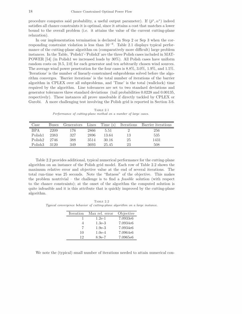
In our implementation termination is declared in Step 2 or Sep 3 when the cor-responding constraint violation is less than 10−6. Table 2.1 displays typical perfor-mance of the cutting-plane algorithm on (comparatively more difficult) large probleminstances. In the Table, ’Polish1’-’Polish3’ are the three Polish cases included in MAT-POWER [54] (in Polish1 we increased loads by 30%). All Polish cases have uniformrandom costs on [0.5, 2.0] for each generator and ten arbitrarily chosen wind sources.The average wind power penetration for the four cases is 8.8%, 3.0%, 1.9%, and 1.5%.’Iterations’ is the number of linearly-constrained subproblems solved before the algo-rithm converges. ’Barrier iterations’ is the total number of iterations of the barrieralgorithm in CPLEX over all subproblems, and ’Time’ is the total (wallclock) timerequired by the algorithm. Line tolerances are set to two standard deviations andgenerator tolerances three standard deviations (tail probabilities 0.0228 and 0.00135,respectively). These instances all prove unsolvable if directly tackled by CPLEX orGurobi. A more challenging test involving the Polish grid is reported in Section 3.6.
Table 2.1
Performance of cutting-plane method on a number of large cases.
Case Buses Generators Lines Time (s) Iterations Barrier iterations
BPA 2209 176 2866 5.51 2 256Polish1 2383 327 2896 13.64 13 535Polish2 2746 388 3514 30.16 25 1431Polish3 3120 349 3693 25.45 23 508
Table 2.2 provides additional, typical numerical performance for the cutting-planealgorithm on an instance of the Polish grid model. Each row of Table 2.2 shows themaximum relative error and objective value at the end of several iterations. Thetotal run-time was 25 seconds. Note the “flatness” of the objective. This makesthe problem nontrivial – the challenge is to find a feasible solution (with respectto the chance constraints); at the onset of the algorithm the computed solution isquite infeasible and it is this attribute that is quickly improved by the cutting-planealgorithm.
Table 2.2
Typical convergence behavior of cutting-plane algorithm on a large instance.
Iteration Max rel. error Objective1 1.2e-1 7.0933e64 1.3e-3 7.0934e67 1.9e-3 7.0934e6
10 1.0e-4 7.0964e612 8.9e-7 7.0965e6
We note the (typical) small number of iterations needed to attain numerical con-
D. Bienstock, M. Chertkov, S. Harnett 19
vergence. Thus at termination only a very small number of conic constraints (2.35)have been incorporated into the master system. This validates the expectation thatonly a small fraction of the conic constraints in CC-OPF are active at optimality. Thecutting-plane algorithm can be viewed as a procedure that opportunistically discoversthese constraints.
2.4. Data-robust chance constraints. Above we developed a formulation forour chance-constrained OPF problem as the conic program (2.29)-(2.37). This ap-proach assumed exact estimates for the mean µi and the variance σ2
i of each windsource ωi. In practice however the estimates at hand might be imprecise7; con-sequently jeopardizing the usefulness of our conic program, henceforth termed thenominal chance-constrained problem. In particular, the performance of the controlcomputed by the conic program might conceivably be sensitive to even small changesin the data. We will deal with this issue in two complimentary ways.
2.4.1. Out-of-sample analysis. Our first approach is the out-of-sample tests,implemented experimentally in Section 3.5. We assume that the µi and σ2
i have beenmis-estimated and explore the robustness of the affine control with respect to theestimation errors. The experiments of Section 3.5 show that the degradation of thechance constraints is small when small data errors are experienced. This empiricalobservation has a rigorous explanation discussed below.
Our chance constraints are represented by convex inequalities, for example inthe case of P (fij > fmax
ij ) < ǫij and P (fij < −fmaxij ) < ǫij we used e.g. (2.34)
and (2.35). Suppose that we have solved the chance-constrained problem assuming(incorrect) expectations µi and variances σ2
i (i ∈ W). Let µi and σ2i (i ∈ W) be the
exact (or realized) values. With some abuse of notation, we will write ξ (resp., ξ) forthe incorrect (exact) distribution. For a given line i, j, write:
mij = Eξfij = βij([B(p + µ − d)]j − [B(p + µ − d)]j), (2.40)
σ2ij = varξfij = β2
ij
∑
k∈W
σ2k(πik − πjk − δi + δj)
2. (2.41)
and similarly,
mij = Eξfij = βij([B(p + µ − d)]j − [B(p + µ − d)]j), (2.42)
σ2ij = varξfij = β2
ij
∑
k∈W
σ2k(πik − πjk − δi + δj)
2. (2.43)
Using (2.42) and (2.43) we see that the “true” probability P (fij > fmaxij ) is that
value ǫ such that
mij + η(ǫ)σij = fmaxij . (2.44)
We wish to evaluate how much larger this (realized) value ǫ is compared with thetarget value ǫij which was the goal in the chance-constrained computation. We willdo this assuming that the estimation errors are small, more precisely, there existnonnegative constants M and V such that
∀i ∈ W, |µi − µi| < Mµi and |σ2i − σ2
i | < V 2σ2i . (2.45)
7In particular since they would effectively be computed in real time.
20 Chance Constrained Optimal Power Flow
Considering Eq. (2.44), we see that for data errors of a given magnitude, ǫ is maximizedwhen mij and σij are maximized. Further, considering Eqs. (2.42) and Eqs. (2.43)we see that to first order mij ≤ mij + O(M), and that σ2
ij ≤ (1 + V 2)σ2ij . From these
two observations and eq. (2.44) we obtain
ǫ =1√2π
∫ +∞
η(ǫ)
e−x2/2dx = ǫij +1√2π
∫ η(ǫij)
η(ǫ)
e−x2/2dx
= ǫij +1√2π
e−η(ǫij )2
2 [η(ǫij) − η(ǫ)] + smaller order errors. (2.46)
The quantity in brackets in the right-hand side of (2.46) equals
η(ǫij) −fmax
ij − mij
σij+
mij − mij
σij< (2.47)
η(ǫij)
(
1 − 1√1 + V 2
)
+mij − mij
σij< (2.48)
η(ǫij)O(V ) +O(M)
σij. (2.49)
Using (2.46) and (2.49) we obtain that ǫ = ǫij + [η(ǫij)O(V )+O(M)]e−η(ǫij )2
2 , wherethe “O” notation contains solution-dependent constants.
2.4.2. Efficiently solvable data-robust formulations. As the preceding anal-ysis makes clear, the constants M and V may need to be quite small, for example ifthe σij are small. We thus seek a better guarantee of robustness. This justifies oursecond approach discussed below – to develop a version of CC-OPF which is method-ologically guaranteed to be insensitive to data errors. This approach puts CC-OPFwithin the scope of robust optimization; to be more precise we will be solving anambiguous chance-constrained problem in the language of [26].
We will write each µi in the form µi + ri, where the µi are point estimates ofthe µi and the ri are “errors” which are constrained to lie in some fixed set M with0 ∈ M. Likewise, we assume that there is a set S ⊆ R
|W| including 0, such that eachσ2
i is of the form σ2i + vi where the vector of errors vi belongs to S. As an example
for how to construct M or S, one can use the following set parameterized by values0 < γi and 0 < Γ:
U(γ, Γ) =
r ∈ RW : |ri| ≤ γi ∀i ∈ W,
∑
i∈W
|ri|γi
≤ Γ
. (2.50)
This set was introduced in [6]. Another candidate is the ellipsoidal set
E(A, b) =
r ∈ R|W| : rT Ar ≤ b
, (2.51)
where A ∈ R|W×W| is positive-definite and b ≥ 0 is a real; see [2], [28]. We can now
formally proceed as follows:
Definitions. Let the estimates µ, σ2 and the sets M and S be given.
D. Bienstock, M. Chertkov, S. Harnett 21
1. For each pair r ∈ M and v ∈ S we will consider a random variable ξ = ξ(r, v)with coordinate-wise mean µ(ξ) = µ + r and variance σ2(ξ) = σ2 + v. We term ξ arealization, and we denote by D = D(µ, M, σ2, S) be the set all realizations.2. A pair p, α is called robust with respect to the pair M, S, if for each line i, j
maxξ∈D
Pξ(fij > fmaxij ) < ǫij , and (2.52)
maxξ∈D
Pξ(fij < −fmaxij ) < ǫij , (2.53)
where we denote by Pξ the probability function under realization ξ.Our task will be to replace, in our optimization problem formulation, the chance
constraint (1.14) with one asking for robustness as in Eqs. (2.52)-(2.53)8. If theuncertainty sets M and S consist of a single point estimate each, then we recover thenominal chance-constrained problem we discussed above. As M or S become larger,the robust approach becomes more insensitive to estimation errors, albeit at the costof becoming more conservative. Thus, a reasonable balance should be attained bychoosing M and S small but of positive measure, thereby preventing trivial sensitivityof the control to changes in the data.
To indicate our approach, we focus on one of the statements for our chance con-straint for lines.
Consider a particular realization ξ ∈ D and denote by θ(ξ) the vector of averagephase angles under ξ (below we will provide an expression for this vector). Robustnesscriterion (2.52) applied to a given line i, j, requires that the chance constraintPξ(fij > fmax
ij ) < ǫij hold. By Lemma 2.4 this statement can be equivalently phrasedas
βij
θi(ξ) − θj(ξ) + η(ǫij)
[
∑
k∈W
σ2k(ξ)(πik − πjk − δi + δj)
2
]1/2
≤ fmaxij .
(2.54)
It follows that robustness criterion (2.52) can be succinctly stated as:
βij maxξ∈D
θi(ξ) − θj(ξ) + η(ǫij)
[
∑
k∈W
σ2k(ξ)(πik − πjk − δi + δj)
2
]1/2
≤ fmaxij .
(2.55)
We can see that (2.55) consists of a (possibly infinite) set of convex constraints;thus the data-robust chance-constrained problem is a convex problem. However weneed to exploit this fact in a computationally favorable manner. Toward this end,our next task is to obtain a more convenient restatement for (2.54). Given a specificξ ∈ D, recall that by definition we have
µ(ξ) = µ + r and σ2(ξ) = σ2 + v (2.56)
for some r ∈ M and v ∈ S. Hence
θ(ξ) = B(p + µ(ξ) − d) = B(p + µ − d) + Br = θ(µ) + Br. (2.57)
8And likewise with the generator chance-constraints (2.36), (2.37).
22 Chance Constrained Optimal Power Flow
Thus, we see that (2.54) can be equivalently rewritten as:
βij(θ(µ)i − θ(µ)j) + βijeTijBr +
η(ǫij)βij
[
∑
k∈W
σ2k(πik − πjk − δi + δj)
2 +∑
k∈W
vk(πik − πjk − δi + δj)2
]1/2
≤ fmaxij . (2.58)
Here, eTij ∈ R
n is the vector with a +1 entry in position i, a -1 entry in position jand 0 elsewhere. In order for (2.52) to hold, (2.58) must hold for all ξ ∈ D, in otherwords, it must hold for all pairs (r, v) with r ∈ M and v ∈ S. It follows that criterion(2.52) can be stated as:
βij(θ(µ)i − θ(µ)j) + βij maxr∈M
eTijBr
+
η(ǫij)βij
[
∑
k∈W
σ2k(πik − πjk − δi + δj)
2 + maxv∈S
∑
k∈W
vk(πik − πjk − δi + δj)2
]1/2
≤ fmaxij . (2.59)
Note that if in the left-hand side of (2.59) we ignore the term involving r andthe second term inside the square brackets, we obtain the nominal (i.e. non-robust)version of chance-constraint (2.52); see Eqs. (2.34), (2.35). A similar constraint (withthe θ terms switched in sign) is obtained from Eqs. (2.53).
Considering eq. (2.59), we see that the maximum over M is independent of alldecision variables and can be computed in advance. In what follows we write, for eachline i, j
Rij.= max
r∈M
eTijBr
. (2.60)
The second maximum in (2.59) presents a challenge. In a traditional robust optimiza-tion approach the next task would be to represent that maximum with an equivalent,compact (i.e. moderate-size) system of equivalent convex constraints. Such a trans-formation would rely on linear programming duality in the case of the uncertaintymodel U(γ, Γ), and on the conic duality or the S-Lemma [12], [28] in the case ofthe ellipsoidal model E(A, b). However, it can be shown that in the case of (2.59)such an approach will fail – it will produce a large formulation, which is additionallynon-convex. We refer the reader to the Appendix for a complete discussion. We nextdescribe an alternate approach that proves efficient.
2.4.3. Efficient solution of the data-robust problem using cutting planes.To derive an algorithm for the data-robust chance-constrained problem that (a) hassome theoretical justification and (b) can prove numerically tractable, we note that ifwe replace the set S with a finite subset S ⊆ S we obtain a valid relaxation for the op-timization problem. In other words the system made-up of the following constraints,for each line i, j,
βij(θ(µ)i − θ(µ)j) + βijRij + βijη(ǫij) sij ≤ fmaxij (2.61)
βij(θ(µ)j − θ(µ)i) − βijRij + βijη(ǫij) sij ≤ fmaxij (2.62)
[
∑
k∈W
(σ2k + vk)(πik − πjk − δi + δj)
2
]1/2
≤ sij ∀ v ∈ S (2.63)
D. Bienstock, M. Chertkov, S. Harnett 23
constitutes a valid relaxation of the chance constraints (2.34), (2.35) of the nominalformulation for each line i, j for any given finite S ⊆ S. This observation can beused to formally obtain a polynomial-time algorithm for the data-robust problem inthe cases of interest. For a given v ∈ S let
Lvij(δ)
.=
(
∑
k∈W
(σ2k + vk)(πik − πjk − δi + δj)
2
)1/2
(i.e., the expression inside the “max” in (2.63).) For completeness, we state thefollowing:
Lemma 2.7. In the case of uncertainty sets of the form U(γ, Γ) or E(A, b) thedata-robust chance-constrained problem can be solved in polynomial time.Proof. Suppose we are given quantities δi for each i ∈ V and sij for each line i, j.Then as argued before, if S is of the form U(γ, Γ) or E(A, b) one can check in polyno-mial time whether maxv∈S
Lvi,j(δ)
≤ sij . If the condition is violated for v ∈ S thentrivially
Lvij(δ) +
∂Lvij(δ)
∂δi(δi − δi) +
∂Lvij(δ)
∂δj(δi − δi) ≤ sij , (2.64)
is violated at δ, s. Since (2.64) is valid for the data-robust chance-constrained problem(by convexity) the result follows by relying on the ellipsoid method [30].
Lemma 2.7 describes a formally “good” algorithm. For computational purposeswe would instead rely on a cutting-plane algorithm much like Algorithm 2.6 developedin Section 2.3. Details are provided in the Appendix.
3. Experiments/Results. Here we will describe qualitative aspects of our affinecontrol on small systems; in particular we focus on the contrast between standard OPF(meaning here and below standard DC OPF) and nominal CC-OPF, on problematicfeatures that can arise because of fluctuating wind sources and on out-of-sample test-ing of the CC-OPF solution, including the analysis of non-Gaussian distributions.Some of our tests involve the BPA grid and Polish Grid, which are large; we presentadditional sets of tests to address the scalability of our solution methodology to thelarge cases. Additional experiments are provided in the Appendix, Section 6.3.
Above (see Eq. (1.8)) we introduced the so-called standard OPF method forsetting traditional generator output levels. When renewables are present, the naturalextension of this approach would make use of some fixed estimate of output (e.g., meanoutput) and to handle fluctuations in renewable output through the same method usedto deal with changes in load: ramping output of traditional generators up or downin proportion to the net increase or decrease in renewable output. This feature couldseamlessly be handled using today’s control structure, with each generator’s outputadjusted at a fixed (preset) rate. For the sake of simplicity, in the experiments belowwe assume that all ramping rates are equal.
Different assumptions on these fixed rates will likely produce different numeri-cal results; however, this general approach entails an inherent weakness. The keypoint here is that mean generator output levels as well as in particular the ramp-ing rates would be chosen without considering the stochastic nature of the renewableoutput levels. Our experiments are designed to highlight the limitations of this “risk-unaware” approach. In contrast, our CC-OPF produces control parameters (the p
24 Chance Constrained Optimal Power Flow
and the α) that are risk-aware and, implicitly, also topology-aware – in the sense ofnetwork proximity to wind farms.
As a technical point, we note that generator adjustment under standard OPFcan be viewed as a special case of our affine control mechanism, but with fixed αvalues. Above, (Lemmas 2.2 and 2.3) we have provided expressions for the mean andstandard deviation of the flow on any given line, under the independence assumptionfor the ωi. It follows that under the Gaussianity assumption, for any given vectors pand α we can compute the probability that any given line i, j is overloaded (bothunder CC-OPF and standard OPF): if z is a standard normal variable, and a > 0,Prob(z > a) = .5 ∗ (1 − erf(z/
√2)), where erf is the error function.
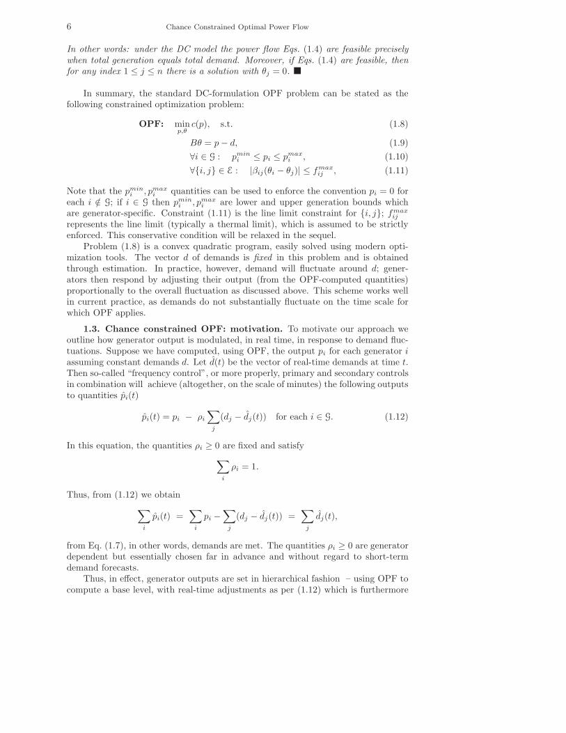
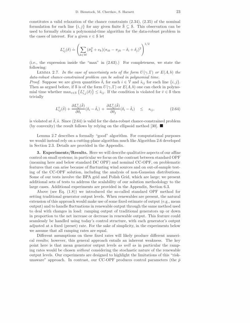
3.1. Failure of standard OPF. We first consider the IEEE 118-bus model witha quadratic cost function, and four sources of wind power added at arbitrary busesto meet 5% of demand in the case of average wind. The standard OPF solution issafely within the thermal capacity limits for all lines in the system. Then we accountfor fluctuations in wind assuming Gaussian and site-independent fluctuations withstandard deviations set to 30% of the respective means. The results, which are shownin Fig. 3.1, illustrate that under standard OPF five lines (marked in red) frequentlybecome overloaded, exceeding their limits 8% or more of the time. This situationtranslates into an unacceptably high risk of failure for any of the five red lines. Thisproblem occurs for grids of all sizes; similar results hold on the 2746-bus Polish grid(from MATPOWER [54]. In this case, after scaling up all loads by 10% to simulatea more highly stressed system, we added wind power to ten buses for a total of 2%penetration. The standard solution results in six lines exceeding their limits over 45%of the time, and in one line over 10% of the time. For an additional and similarexperiment using the Polish grid see Section 3.6.
3.2. Cost of reliability under high wind penetration. If we stay withincurrent operational paradigm, congestion of transmission lines may force temporaryshutdown of wind farms even during times of high wind. Our methodology suggests, asan alternative solution to curtailment of wind power, an appropriate reconfigurationof standard generators. If successful, this solution can use the available wind powerwithout curtailment, and thus result in cheaper operating costs.
As a (crude) proxy for curtailment, we perform the following experiment, whichconsiders different levels of renewable penetration. Here, the mean power outputs ofthe wind sources are kept in a fixed proportion to one another and proportionallyscaled so as to vary total amount of penetration, and likewise with the standarddeviations. First, we run our CC-OPF under a high penetration level (e.g., 30%).Under this penetration level, the standard OPF solution yields very high probabilityof line overloads. In order to obtain a comparison with CC-OPF, we increase line limitsby 10% while simultaneously reducing wind penetration (i.e., curtail wind) so thatunder the standard OPF solution line overloads are reduced to an acceptable level.Assuming zero cost for wind power, the difference in cost for the high-penetrationCC-OPF solution and the low-penetration standard solution represents the savingsproduced by our model (generously, given the 10% line limit increase).
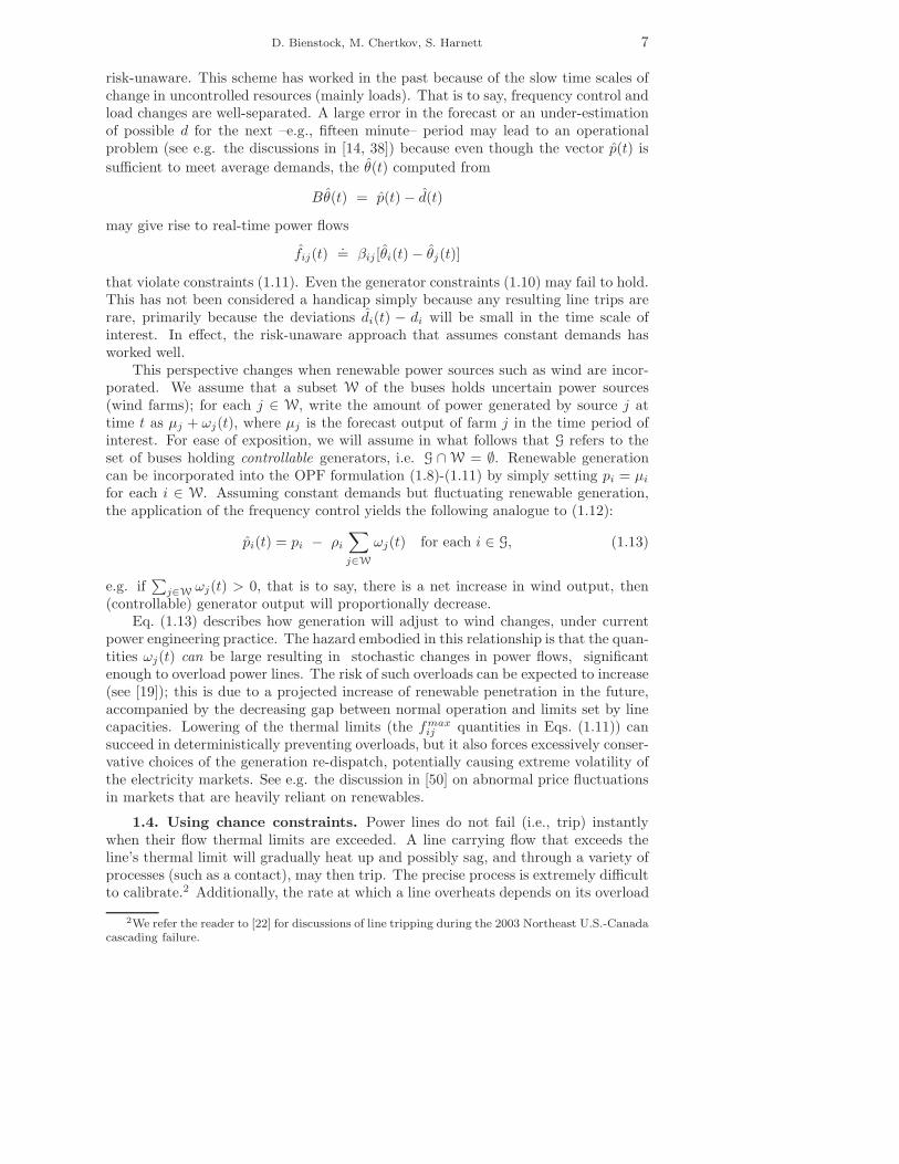
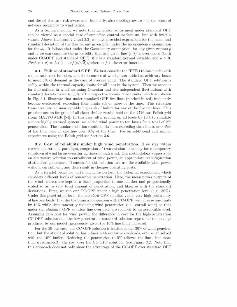
For the 39-bus case, our CC-OPF solution is feasible under 30% of wind penetra-tion, but the standard solution has 5 lines with excessive overloads, even when solvedwith the 10% buffer. Reducing the penetration to 5% relieves the lines, but morethan quadruples(!) the cost over the CC-OPF solution. See Figure 3.2. Note thatthis approach does not only show the advantage of the CC-OPF over standard OPF
D. Bienstock, M. Chertkov, S. Harnett 25
Fig. 3.1. 118-bus case with four wind farms (green dots; brown are generators, black are loads).Shown is the standard OPF solution against the average wind case with penetration of 5%. Standarddeviations of the wind are set to 30% of the respective average cases. Lines in red exceed their limit8% or more of the time.
but also provides a quantitative measure of the advantage, thus placing a well-definedprice tag on reliability.
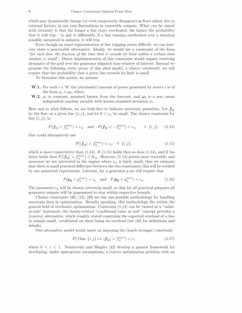
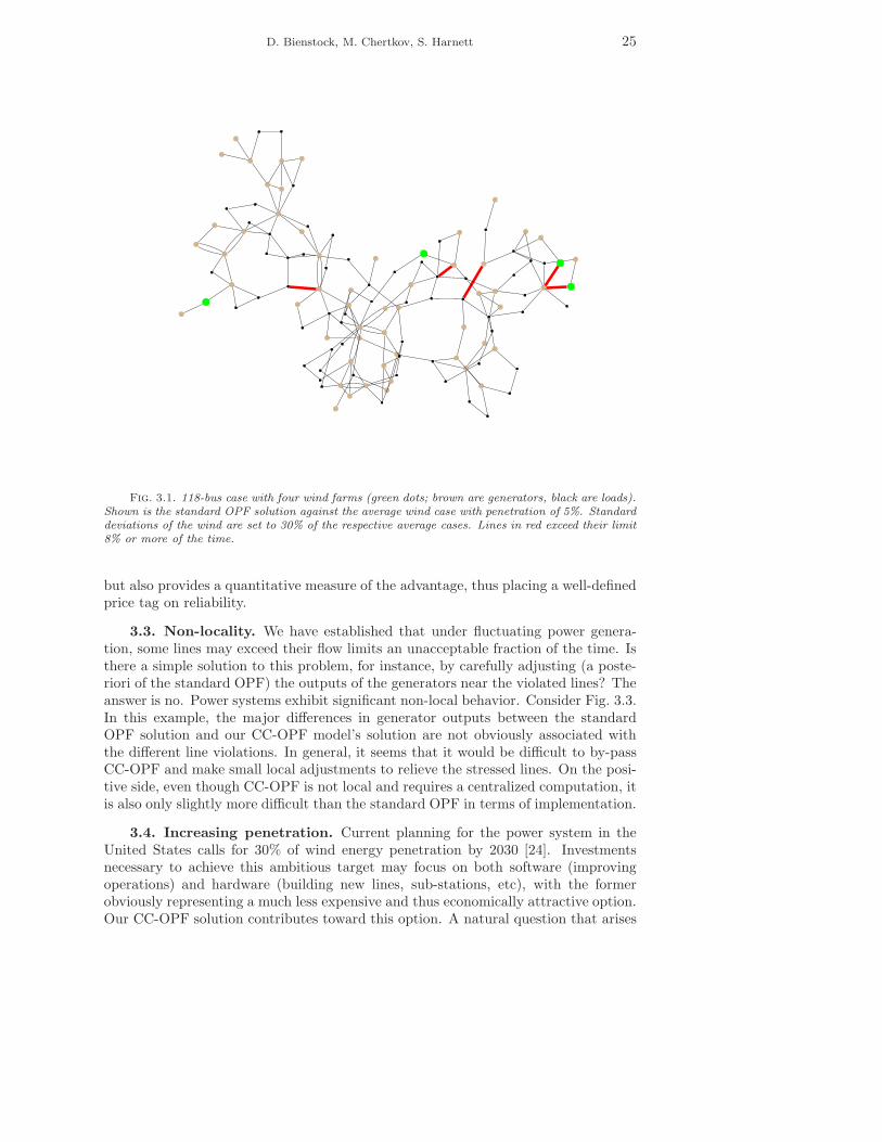
3.3. Non-locality. We have established that under fluctuating power genera-tion, some lines may exceed their flow limits an unacceptable fraction of the time. Isthere a simple solution to this problem, for instance, by carefully adjusting (a poste-riori of the standard OPF) the outputs of the generators near the violated lines? Theanswer is no. Power systems exhibit significant non-local behavior. Consider Fig. 3.3.In this example, the major differences in generator outputs between the standardOPF solution and our CC-OPF model’s solution are not obviously associated withthe different line violations. In general, it seems that it would be difficult to by-passCC-OPF and make small local adjustments to relieve the stressed lines. On the posi-tive side, even though CC-OPF is not local and requires a centralized computation, itis also only slightly more difficult than the standard OPF in terms of implementation.
3.4. Increasing penetration. Current planning for the power system in theUnited States calls for 30% of wind energy penetration by 2030 [24]. Investmentsnecessary to achieve this ambitious target may focus on both software (improvingoperations) and hardware (building new lines, sub-stations, etc), with the formerobviously representing a much less expensive and thus economically attractive option.Our CC-OPF solution contributes toward this option. A natural question that arises
26 Chance Constrained Optimal Power Flow
Fig. 3.2. 39-bus case under standard solution. Even with a 10% buffer on the line flow limits,five lines exceed their limit over 5% of the time with 30% penetration (left). The penetration mustbe decreased to 5% before the lines are relieved, but at great cost (right). The CC-OPF model isfeasible for 30% penetration at a cost of 264,000. The standard solution at 5% penetration costs1,275,020 – almost 5 times as much.
Fig. 3.3. 39-bus case. Red lines indicate high probability of flow exceeding the limit underthe standard OPF solution. Generators are shades of blue, with darker shades indicating greaterabsolute difference between the chance-constrained solution and the standard solution.
concerns the maximum level of penetration one can safely achieve by upgrading fromthe standard OPF to our CC-OPF.
To answer the question we consider the 39-bus New England system (from [54])case with four wind generators added, and line flow limits scaled by .7 to simulate aheavily loaded system. The quadratic cost terms are set to rand(0,1) + .5. We fix thefour wind generator average outputs in a ratio of 5/6/7/8 and standard deviations at30% of the mean. We first solve our model using ǫ = .02 for each line and assumingzero wind power, and then increase total wind output until the optimization problembecomes infeasible. See Figure 3.4. This experiment illustrates that at least forthe model considered, the 30% of wind penetration with rather strict probabilisticguarantees enforced by our CC-OPF may be feasible, but in fact lies rather close tothe dangerous threshold. To push penetration beyond the threshold is impossiblewithout upgrading lines and investing in other (not related to wind farms themselves)
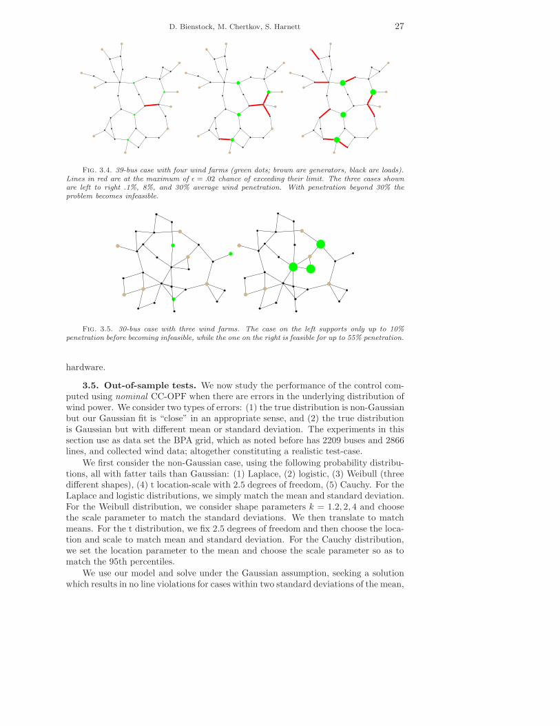
D. Bienstock, M. Chertkov, S. Harnett 27
Fig. 3.4. 39-bus case with four wind farms (green dots; brown are generators, black are loads).Lines in red are at the maximum of ǫ = .02 chance of exceeding their limit. The three cases shownare left to right .1%, 8%, and 30% average wind penetration. With penetration beyond 30% theproblem becomes infeasible.
Fig. 3.5. 30-bus case with three wind farms. The case on the left supports only up to 10%penetration before becoming infeasible, while the one on the right is feasible for up to 55% penetration.
hardware.
3.5. Out-of-sample tests. We now study the performance of the control com-puted using nominal CC-OPF when there are errors in the underlying distribution ofwind power. We consider two types of errors: (1) the true distribution is non-Gaussianbut our Gaussian fit is “close” in an appropriate sense, and (2) the true distributionis Gaussian but with different mean or standard deviation. The experiments in thissection use as data set the BPA grid, which as noted before has 2209 buses and 2866lines, and collected wind data; altogether constituting a realistic test-case.
We first consider the non-Gaussian case, using the following probability distribu-tions, all with fatter tails than Gaussian: (1) Laplace, (2) logistic, (3) Weibull (threedifferent shapes), (4) t location-scale with 2.5 degrees of freedom, (5) Cauchy. For theLaplace and logistic distributions, we simply match the mean and standard deviation.For the Weibull distribution, we consider shape parameters k = 1.2, 2, 4 and choosethe scale parameter to match the standard deviations. We then translate to matchmeans. For the t distribution, we fix 2.5 degrees of freedom and then choose the loca-tion and scale to match mean and standard deviation. For the Cauchy distribution,we set the location parameter to the mean and choose the scale parameter so as tomatch the 95th percentiles.
We use our model and solve under the Gaussian assumption, seeking a solutionwhich results in no line violations for cases within two standard deviations of the mean,
28 Chance Constrained Optimal Power Flow
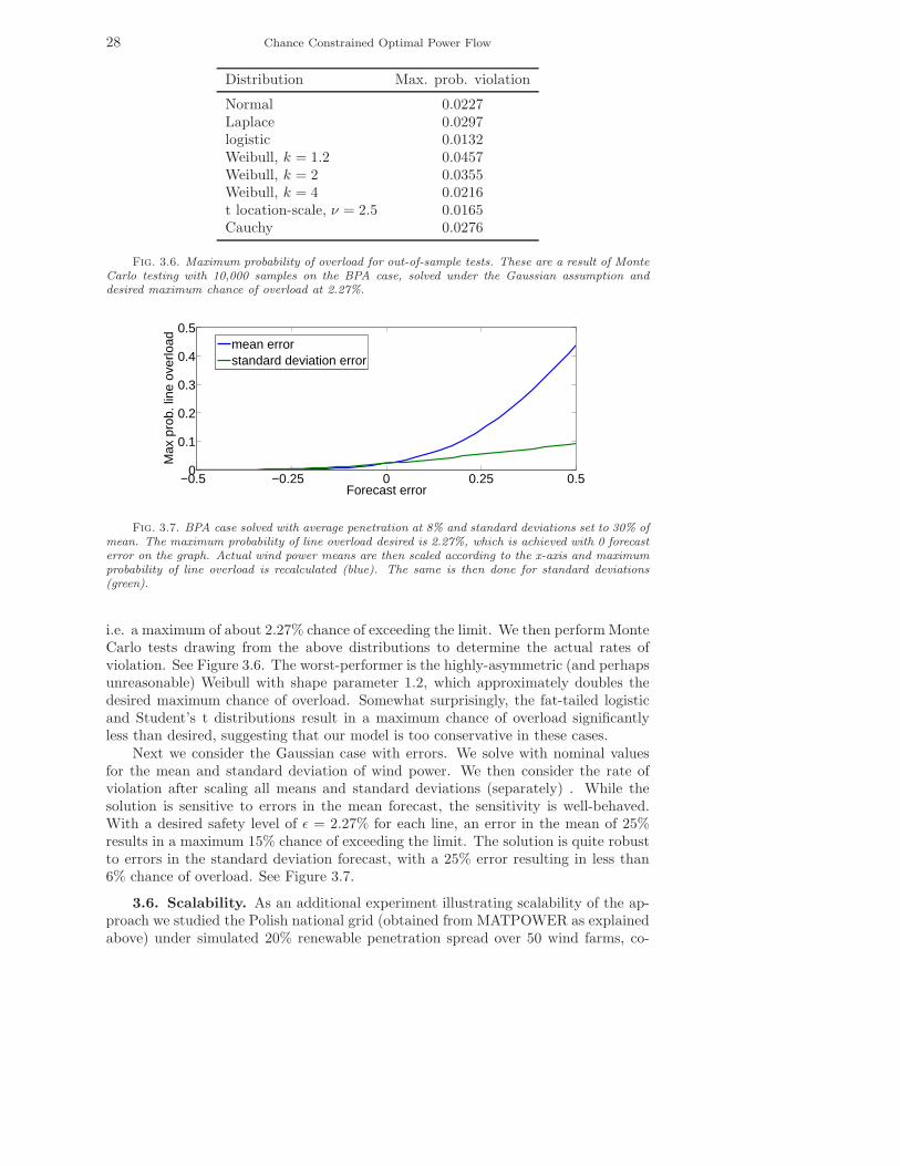
Distribution Max. prob. violation
Normal 0.0227Laplace 0.0297logistic 0.0132Weibull, k = 1.2 0.0457Weibull, k = 2 0.0355Weibull, k = 4 0.0216t location-scale, ν = 2.5 0.0165Cauchy 0.0276
Fig. 3.6. Maximum probability of overload for out-of-sample tests. These are a result of MonteCarlo testing with 10,000 samples on the BPA case, solved under the Gaussian assumption anddesired maximum chance of overload at 2.27%.
−0.5 −0.25 0 0.25 0.50
0.1
0.2
0.3
0.4
0.5
Forecast error
Max
pro
b. li
ne o
verlo
ad
mean errorstandard deviation error
Fig. 3.7. BPA case solved with average penetration at 8% and standard deviations set to 30% ofmean. The maximum probability of line overload desired is 2.27%, which is achieved with 0 forecasterror on the graph. Actual wind power means are then scaled according to the x-axis and maximumprobability of line overload is recalculated (blue). The same is then done for standard deviations(green).
i.e. a maximum of about 2.27% chance of exceeding the limit. We then perform MonteCarlo tests drawing from the above distributions to determine the actual rates ofviolation. See Figure 3.6. The worst-performer is the highly-asymmetric (and perhapsunreasonable) Weibull with shape parameter 1.2, which approximately doubles thedesired maximum chance of overload. Somewhat surprisingly, the fat-tailed logisticand Student’s t distributions result in a maximum chance of overload significantlyless than desired, suggesting that our model is too conservative in these cases.
Next we consider the Gaussian case with errors. We solve with nominal valuesfor the mean and standard deviation of wind power. We then consider the rate ofviolation after scaling all means and standard deviations (separately) . While thesolution is sensitive to errors in the mean forecast, the sensitivity is well-behaved.With a desired safety level of ǫ = 2.27% for each line, an error in the mean of 25%results in a maximum 15% chance of exceeding the limit. The solution is quite robustto errors in the standard deviation forecast, with a 25% error resulting in less than6% chance of overload. See Figure 3.7.
3.6. Scalability. As an additional experiment illustrating scalability of the ap-proach we studied the Polish national grid (obtained from MATPOWER as explainedabove) under simulated 20% renewable penetration spread over 50 wind farms, co-
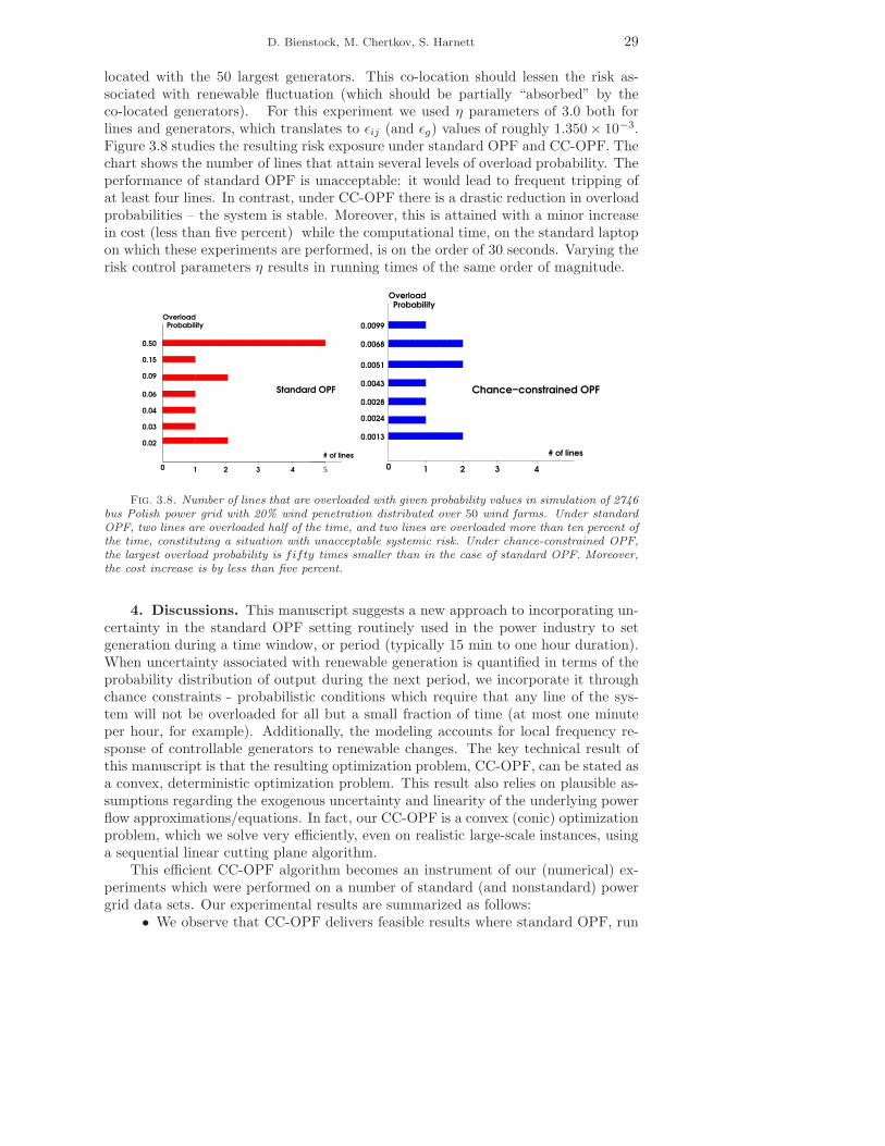
D. Bienstock, M. Chertkov, S. Harnett 29
located with the 50 largest generators. This co-location should lessen the risk as-sociated with renewable fluctuation (which should be partially “absorbed” by theco-located generators). For this experiment we used η parameters of 3.0 both forlines and generators, which translates to ǫij (and ǫg) values of roughly 1.350 × 10⁻³.Figure 3.8 studies the resulting risk exposure under standard OPF and CC-OPF. Thechart shows the number of lines that attain several levels of overload probability. Theperformance of standard OPF is unacceptable: it would lead to frequent tripping ofat least four lines. In contrast, under CC-OPF there is a drastic reduction in overloadprobabilities – the system is stable. Moreover, this is attained with a minor increasein cost (less than five percent) while the computational time, on the standard laptopon which these experiments are performed, is on the order of 30 seconds. Varying therisk control parameters η results in running times of the same order of magnitude.
1 2 3 40
ProbabilityOverload
Standard OPF
# of lines
5
0.50
0.09
0.15
0.06
0.04
0.03
0.02
1 3 40
ProbabilityOverload
# of lines
Chance−constrained OPF
2
0.0099
0.0068
0.0051
0.0043
0.0028
0.0024
0.0013
Fig. 3.8. Number of lines that are overloaded with given probability values in simulation of 2746bus Polish power grid with 20% wind penetration distributed over 50 wind farms. Under standardOPF, two lines are overloaded half of the time, and two lines are overloaded more than ten percent ofthe time, constituting a situation with unacceptable systemic risk. Under chance-constrained OPF,the largest overload probability is fifty times smaller than in the case of standard OPF. Moreover,the cost increase is by less than five percent.
4. Discussions. This manuscript suggests a new approach to incorporating un-certainty in the standard OPF setting routinely used in the power industry to setgeneration during a time window, or period (typically 15 min to one hour duration).When uncertainty associated with renewable generation is quantified in terms of theprobability distribution of output during the next period, we incorporate it throughchance constraints - probabilistic conditions which require that any line of the sys-tem will not be overloaded for all but a small fraction of time (at most one minuteper hour, for example). Additionally, the modeling accounts for local frequency re-sponse of controllable generators to renewable changes. The key technical result ofthis manuscript is that the resulting optimization problem, CC-OPF, can be stated asa convex, deterministic optimization problem. This result also relies on plausible as-sumptions regarding the exogenous uncertainty and linearity of the underlying powerflow approximations/equations. In fact, our CC-OPF is a convex (conic) optimizationproblem, which we solve very efficiently, even on realistic large-scale instances, usinga sequential linear cutting plane algorithm.
This efficient CC-OPF algorithm becomes an instrument of our (numerical) ex-periments which were performed on a number of standard (and nonstandard) powergrid data sets. Our experimental results are summarized as follows:
• We observe that CC-OPF delivers feasible results where standard OPF, run
30 Chance Constrained Optimal Power Flow
for the average forecast, would fail in the sense that many lines would beoverloaded an unacceptably large portion of time.
• Not only is CC-OPF safer than standard OPF, but it also results in cheaperoperation. This is demonstrated by considering the optimal cost of CC-OPFunder sufficiently high wind penetration solution (where standard OPF wouldfail) and the low penetration solution (corresponding to the highest possiblepenetration where standard OPF would not fail).
• We discover that solutions produced by CC-OPF deviate significantly fromwhat amounts to a naive adjustment of the standard OPF obtained by cor-recting dispatch just at those generators which are close to overloaded lines.
• We test the level of wind penetration which can be tolerated without upgrad-ing lines. This experiment illustrates that, at least for the model tested, the30% of wind penetration with rather strict probabilistic guarantees enforcedby our CC-OPF may be feasible; but much lower wind penetration remainsfeasible under the standard approach.
• We experiment with location of wind farms and discover strong sensitivity ofthe maximum level of penetration on the choice of location - optimal choiceof wind farm location is critical for achieving the ambitious goal of highrenewable penetration.
• Analyzing fluctuations of line flows within CC-OPF solution admissible underhigh wind penetration, we discover that these fluctuations may be significant,in particular resulting in reversal of power flows over some of the lines. Thisobservation suggests that flow reversals and other qualitative changes of powerflows, which are extremely rare in the grid of today, will become significantlymuch more frequent (typical) in the grid of tomorrow.
• We studied an out-of-sample test consisted in applying CC-OPF (modelingexogenous fluctuations as Gaussian) to other distributions. Overall these testssuggest that with a proper calibration of the effective Gaussian distributionour CC-OPF delivers a rather good performance. One finds that the worstCC-OPF performance is observed for the most asymmetric distributions.
• We also presented a computationally sound data-robust version of the CC-OPF where the parameters for the Gaussian distributions are assumed un-known, but lying in a window. This allows for parameter mis-estimation,for model error, and it is suggests a way to deal in a tractable way withnon-Gaussian fluctuations.
The nature of the problem discussed in the manuscript – the design of a newparadigm for computationally efficient generation re-dispatch that accounts for windfluctuations – inevitably required incorporation of a number of assumptions and ap-proximations. In particular, we made simplifying assumptions about static forecastsand general validity of power flow linearization. We have also focused solely on fail-ures associated with line congestion ignoring other possible difficulties, for examplethose associated with loss of synchronicity and voltage variations. However, we wouldlike to emphasize that all of these assumptions (admittedly natural for a first attackon the problem) also allow generalization within the approach just sketched:
• Accounting for time evolving forecast/loads/etc. Wind forecast, expressed interms of the mean and standard deviation at the wind farm sites, changeson the scales comparable to duration of the generation re-dispatch interval.Loads may also change at these time scales. When the slowly evolving, butstill not constant, wind and load forecasts are available we may keep the

D. Bienstock, M. Chertkov, S. Harnett 31
quasi-static power flow description and incorporate this slow evolution intime into the chance constrained scheme. These changes will simply result ingeneralizing the conic formulation (2.29)-(2.37) by splitting what used to bea single time interval into sub-intervals and allowing the regular generation tobe re-dispatched and parallel coefficients to be adjusted more often. Rampingrate constraints on the controllable generation may naturally be accountedin the temporal optimization scheme as well.
• Accounting for nonlinearity in power flows. Evolution of the base case in-validates the approximate linear model. However, one may simply adjustthe approximate linear models in a number of steps, therefore incorporatingit into the dynamical procedure mentioned one item above. Additionally,some interesting new methodologies for handling nonlinearities have recentlyemerged, see [37].
• Accounting for synchronization bounds. Loss of synchronicity and resultingdisintegration of the grid is probably the most acute contingency which canpossibly take place in a power system. The prediction of those conditionsunder which the power grid will lose synchronicity is a difficult nonlinear anddynamic problem. However, as shown recently in [23], one can formulate anaccurate linear and static necessary condition for the loss of synchronicity.A chance-constrained version of the linear synchronization conditions can beincorporated seamlessly in our CC-OPF framework.
Finally, we see many opportunities in utilizing the CC-OPF (possibly modified) asan elementary unit or an integral part of even more complex problems, such as com-bined unit commitment (scheduling large power plants normally days, weeks or evenmonths ahead) [51] with CC-OPF, planning grid expansion [3] while accounting forcost operation under uncertainty, or incorporating CC-OPF in mitigating emergencyof possible cascades of outages [16, 41, 45, 44, 8, 9, 25, 5]. In this context, it would beadvantageous to speed up our already very efficient CC-OPF even further. See, forexample, [10], [7]. A different methodology, relying on distributed algorithms, can befound in [35].
5. Acknowledgments. We are thankful to S. Backhaus and R. Bent for theircomments, and to K. Dvijotham for help with BPA data. The work at LANL wascarried out under the auspices of the National Nuclear Security Administration ofthe U.S. Department of Energy at Los Alamos National Laboratory under ContractNo. DE-AC52-06NA25396. MC and SH also acknowledge partial support of theDTRA Basic Research grant BRCALL08-Per3-D-2-0022. DB and SH were partiallysupported by DOE award DE-SC0002676.
The authors would like to acknowledge two recent preprints [48, 47], discussingrelated in general, but different in details (in particular, in what concern formulationand efficient implementation) CC-OPF ideas. The authors became aware of thesepreprints after posting the first version of this manuscript online.
REFERENCES
[1] S. Baghsorkhi and I. Hiskens, Analysis tools for assessing the impact of wind power on weakgrids, SysCon, (2012), pp. 1 –8.
[2] R. Ben-Tal and A. Nemirovski, Robust solutions of linear programming problems contami-nated with uncertain data, Mathematical Programming, 88 (2000), pp. 411–424.
[3] R. Bent, G. Toole, and A. Berscheid, Transmission network expansion planning with com-plex power flow models, Power Systems, IEEE Transactions on, 27 (2012), pp. 904 –912.

32 Chance Constrained Optimal Power Flow
[4] A. Bergen and V. Vittal, Power System Analysis, Prentice Hall. Inc, 2000.[5] A. Bernstein, D. Hay, M. Uzunoglu, and G. Zussman, Power grid vulnerability to geo-
graphically correlated failures - analysis and control implications. http://arxiv.org/abs/1206.1099, 2012.
[6] D. Bertsimas and M. Sim, Price of robustness, Operations Research, 52 (2004), pp. 35–53.[7] D. Bienstock, Potential Function Methods for Approximately Solving Linear Programming
Problems, Theory and Practice, Kluwer, 2002.[8] D. Bienstock, Adaptive online control of cascading blackouts, Proc. 2011 IEEE Power and
Energy Society General Meeting, (2011), pp. 1–8.[9] , Optimal control of cascading power grid failures, Proc 2011 CDC-ECC, (2011), pp. 2166
–2173.[10] D. Bienstock and G. Iyengar, Faster approximation algorithms for covering and packing
problems, SIAM Journal on Computing, 35 (2006), pp. 825–854.[11] H. Bludszuweit, J. Dominguez-Navarro, and A. Llombart, Statistical analysis of wind
power forecast error, Power Systems, IEEE Transactions on, 23 (2008), pp. 983 –991.[12] S. Boyd and L. Vandenberghe, Convex Optimization, Cambridge University Press, 2004.[13] BPA-WIND, Wind generation & total load in the bpa balancing authority. http://
transmission.bpa.gov/business/operations/wind/, 2012.[14] CAISO, Integration of renewable resources: Transmission and operating issues and rec-
ommendations for integrating renewable resources on the california iso-controlled grid.http://www.caiso.com/1ca5/1ca5a7a026270.pdf, 2007.
[15] A. Charnes, W. Cooper, and G. Symonds, Cost horizons and certainty equivalents: anapproach to stochastic programming of heating oil, Management Science, 4 (1958), pp. 235–263.
[16] J. Chen, J. Thorp, and I. Dobson, Cascading dynamics and mitigation assessment in powersystem disturbances via a hidden failure model, International Journal of Electrical Power;Energy Systems, 27 (2005), pp. 318 – 326.
[17] M. Chertkov, F. Pan, and M. Stepanov, Predicting failures in power grids: The case ofstatic overloads, IEEE Transactions on Smart Grids, 2 (2010), p. 150.
[18] M. Chertkov, M. Stepanov, F. Pan, and R. Baldick, Exact and efficient algorithm todiscover extreme stochastic events in wind generation over transmission power grids, CDC-ECC, (2011), pp. 2174 –2180.
[19] CIGRE, Technical brochure on grid integration of wind generation, International Conferenceon Large High Voltage Electric Systems, (2009).
[20] CPLEX, ILOG CPLEX Optimizer. http://www-01.ibm.com/software/integration/
optimization/cplex-optimizer/, 2012.[21] DENA, Energy management planning for the integration of wind energy into the grid in ger-
many, onshore and offshore by 2020, 2005.[22] DOE-Report, U.s.-canada power system outage task force. report on the august 14,
2003 blackout in the united states and canada: Causes and recommendations.https://reports.energy.gov, (2004).
[23] F. Dorfler, M. Chertkov, and F. Bullo, Synchronization in Complex Oscillator Networksand Smart Grids, Proceedings of National Academy of Sciences, 10.1073/pnas.1212134110(2013).
[24] EERE, 20% of wind energy by 2030: Increasing wind energy’s contribution to us electricitysupply, Department of Energy (DOE), DOE/GO-102008-2567 (2008).
[25] M. Eppstein and P. Hines, A ”random chemistry” algorithm for identifying collections ofmultiple contingencies that initiate cascading failure, Power Systems, IEEE Transactionson, 27 (2012), pp. 1698–1705.
[26] E. Erdogan and G. Iyengar, Ambiguous chance constrained problems and robust optimiza-tion, Mathematical Programming, 107 (2007), pp. 37–61.
[27] D. Goldfarb and F. Alizadeh, Second-order cone programming, Mathematical Programming,95 (2003), pp. 3–51.
[28] D. Goldfarb and G. Iyengar, Robust portfolio selection problems, Mathematical Program-ming, 28 (2001), pp. 1–38.
[29] G. Gonzalez and et al., Experience integrating and operating wind power in the peninsularspanish power system. point of view of the transmission system operator and a wind powerproducer, CIGRE, (2006).
[30] M. Grotschel, L. Lovasz, and A. Schrijver, Geometric Algorithms and CombinatorialOptimization, Springer-Verlag, 1998.
[31] GUROBI, Optimizer. http://www.gurobi.com/, 2012.[32] B.-M. Hodge and M. Milligan, Wind power forecasting error distributionsover multiple
D. Bienstock, M. Chertkov, S. Harnett 33
timescales, Detroit Power Engineering Society Meeting, (2011), pp. 1–8.[33] M. Huneault, A survey of the optimal power flow literature, Power Systems, IEEE Transac-
tions, (1991).[34] J. E. Kelley, The cutting-plane method for solving convex programs, Journal of the Society
for Industrial and Applied Mathematics, 8 (1960), pp. 703–712.[35] M. Kraning, E. Chu, J. Lavaei, and S. Boyd, Message passing for dynamic network energy
management. http://www.stanford.edu/~boyd/papers/decen_dyn_opt.html, 2012.[36] P. Kundur, Power System Stability and Control, McGraw-Hill, New York, NY, USA, 1994.[37] J. Lavaei and S. Low, Zero duality gap in optimal power flow problem, IEEE Transactions on
Power Systems, 27 (2012), pp. 92–107.[38] Y. Makarov, C. Loutan, J. Ma, and P. de Mello, Operational impacts of wind generation
on california power systems, Power Systems, IEEE Transactions on, 24 (2009), pp. 1039–1050.
[39] L. Miller and H. Wagner, Chance-constrained programming with joint constraints, Opera-tions Research, 13 (1965), pp. 930–945.
[40] MOSEK, Optimizer. http://www.mosek.com/, 2012.[41] D. Nedic, I. Dobson, D. Kirschen, B. Carreras, and V. E. Lynch, Criticality in a cascad-
ing failure blackout model, International Journal of Electrical Power; Energy Systems, 28(2006), pp. 627 – 633.
[42] A. Nemirovski and A. Shapiro, Convex approximations of chance constrained programs,SIAM Journal on Optimization, 17 (2006), pp. 969–996.
[43] U. Ozturk and M. Mazumdar, A solution to the stochastic unit commitment problem usingchance constrained programming, Power Systems, IEEE, 19 (2004), pp. 1589–1598.
[44] R. Pfitzner, K. Turitsyn, and M. Chertkov, Controlled Tripping of Overheated LinesMitigates Power Outages, arxiv:1104.4558, (2011).
[45] R. Pfitzner, K. Turitsyn, and M. Chertkov, Statistical classification of cascading failuresin power grids, in Power and Energy Society General Meeting, 2011 IEEE, july 2011, pp. 1–8.
[46] A. Prekopa, On probabilistic constrained programming, Proc. Princeton Symposium on Math.Programming, (1970), pp. 113–138.
[47] L. Roald, F. Oldewurtel, T. Krause, and G. Andersson, Analytical reformulation ofsecurity constrained optimal power flow with probabilistic constraints, in Proceedings ofthe Grenoble PowerTech, Grenoble, France, 2013.
[48] A. Sjodin, D. Gayme, and U. Topcu, Risk-mitigated optimal power flow with high windpenetration. http://smart.caltech.edu/papers/riskoptimal.pdf, 2012.
[49] M. Vrakopoulou, K. Margellos, J. Lygeros, and G. Andersson, A probabilistic frameworkfor security constrained reserve scheduling of networks with wind power generation, inEnergy Conference and Exhibition (ENERGYCON), 2012 IEEE International, sept. 2012,pp. 452 –457.
[50] G. Wang, M. Negrete-Pincetic, A. Kowli, E. Shafieepoorfard, S. Meyn, and
U. Shanbhag, Dynamic competitive equilibria in electricity markets, in Control and Op-timization Theory for Electric Smart Grids, A. Chakrabortty and M. Illic, eds., Springer,2011.
[51] J. Wang, M. Shahidehpour, and Z. Li, Security-constrained unit commitment with volatilewind power generation, Power Systems, IEEE Transactions on, 23 (2008), pp. 1319 –1327.
[52] H. Zhang, Chance Constrained Programming for Optimal Power Flow Under Uncertainty,Power Systems, IEEE Transactions on, 26 (2011), pp. 2417–2424.
[53] S. Zhang, Y. Song, Z. Hu, and L. Yao, Robust optimization method based on scenario analysisfor unit commitment considering wind uncertainties, in Power and Energy Society GeneralMeeting, 2011 IEEE, july 2011, pp. 1 –7.
[54] R. Zimmerman, C. Murillo-Sanchez, and R. Thomas, Matpower: Steady-state operations,planning, and analysis tools for power systems research and education, Power Systems,IEEE Transactions on, 26 (2011), pp. 12 –19.
6. Appendix.
6.1. Data-robust algorithm. Here we provide a description of our data-robustapproach for the CC-OPF problem discussed in Section 2.4.3. Our first task is toincorporate constraint (2.59) into an efficient solution procedure. To motivate ourapproach, we will first show that a methodology based on traditional robust opti-mization techniques will (likely) not succeed at this task. We will then describe the
34 Chance Constrained Optimal Power Flow
method we rely on.Constraint (2.59) can be incorporated into a formulation provided we can appro-
priately represent the two maxima. Here, note that
mij.= max
r∈M
eTijBr
, (6.1)
is independent of all variables and can be solved beforehand for all lines (i, j); whenM is of the form U(γ, Γ) given above this is a linear programming problem and whenM = E(A, b) the task amounts to finding a point in the boundary of an ellipsoidwith normal parallel to a given vector and thus requires solving a linear system ofequations. We will likewise define a quantity mji using eji instead of eij .
It is the second maximization that presents some challenges.Lemma 6.1. Suppose S = U(γ, Γ), and suppose a vector δ ∈ Rn is given. Then
maxv∈S
∑
k∈W
vk(πik − πjk − δi + δj)2
= min Γa +∑
k∈W
γkbk
s.t.1
γka + bk ≥ (πik − πjk − δi + δj)
2 ∀ k ∈ W,
bk ≥ 0 ∀ k ∈ W; a ≥ 0.
Proof. Since (πik − πjk − δi + δj)2 ≥ 0 without loss of generality in the maximum we
will have that vk ≥ 0 for all k. Thus, we can rewrite the maximum as
max∑
k∈W
vk(πik − πjk − δi + δj)2
s.t.∑
k∈W
1
γkvk ≤ Γ (6.2)
vk ≤ γk ∀ k ∈ W, (6.3)
0 ≤ v. (6.4)
This is a linear program; denoting by a the dual variable for (6.2) and by bk that for(6.3), strong linear programming duality now gives the result.
The use of linear programming duality as in Lemma 6.1 is key in the context ofsets of the form U(γ, Γ). In the case of an ellipsoidal set E(A, b) as in (2.51) there isan analogue to Lemma 6.1 that instead uses the S-Lemma [12], [28]. In the standardrobust optimization approach, Lemma 6.1 would be leveraged to produce a result ofthe following type:
Lemma 6.2. Suppose S = U(γ, Γ). The data-robust chance-constrained problemis obtained by replacing for each line (i, j) constraints (2.34), (2.35) of the nominalformulation with
βij(θ(µ)i − θ(µ)j) + βijmij + βijη(ǫij) sij ≤ fmaxij (6.5)
βij(θ(µ)j − θ(µ)i) + βijmji + βijη(ǫij) sij ≤ fmaxij (6.6)
[
∑
k∈W
σ2k(πik − πjk − δi + δj)
2 + Γai,j +∑
k∈W
bi,jk
]1/2
≤ sij (6.7)
(πik − πjk − δi + δj)2 − 1
γkai,j − b
i,jk ≤ 0 ∀k ∈ W (6.8)
bi,jk ≥ 0 ∀k ∈ W; ai,j ≥ 0. (6.9)
D. Bienstock, M. Chertkov, S. Harnett 35
Here, si,j , ai,j and bi,jk (k ∈ W) are additional variables.
Proof sketch. Without loss of generality at the optimum the ai,j and bi,jk are
chosen so as to minimize the left-hand side of (6.7) subject to all other variables heldfixed, thereby obtaining the “min” in Lemma 6.1.
Lemma 6.2 points out the difficulty that the standard robust optimization ap-proach would engender in the context of our problem. First, the number of constraints(6.7) and (6.8) is large: it equals |E|(1+ |W|) and thus in the case of a large transmis-sion system it could approach many tens of thousands (or more). Thus, even thoughwe obtain a compact formulation (i.e., of polynomial size) it is likely to be proven toolarge for present-day solvers. But there is a second and more fundamental problem:constraint (6.7) is not convex. This is a significant methodological difficulty. A similarset of hurdles arises when using uncertainty sets E(A, b).
6.2. Cutting-plane algorithm for the data-robust problem. Here we de-scribe a cutting-plane algorithm for the data-robust version of the CC-OPF problem,akin to Algorithm 2.6 used in Section 2.3 to solve the nominal (known data) case.
In the following description for brevity we assume that only line-limit chanceconstraints are incorporated (no generator-related chance constraints).
Procedure 6.3. CUTTING-PLANE ALGORITHM FOR DATA-ROBUSTPROBLEM
Initialization: The linear “master” system A(p, α, δ, θ, s)T ≥ b is defined toinclude constraints (2.30)-(2.34). For each line (i, j) compute the Rij parametersdefined in (2.60).
Iterate:
(1) Solve minF (p, α) : A(p, α, δ, θ, s)T ≥ b. Let (p∗, α∗, δ∗, θ∗, s∗) bean optimal solution.
(2) For each line (i, j) compute
V ∗ij
.= max
v∈S
∑
k∈W
vk(πik − πjk − δ∗i + δ∗j )2
,
with solution v = v(δ∗) ∈ S.
(3) If, for each line i, j,[
V ∗ij
]1/2 ≤ s∗ij , (within tolerance) Stop.
(4) Otherwise, add to the master system inequality (2.64).
Clearly the algorithm always maintains a valid (linear) relaxation to the data-robustoptimization problem – this follows because (2.64) is simply an outer approxima-tion (tangent hyperplane) to one of the conic sets defined by (2.63). Thus, in addi-tion, the stopping criterion in (3) is valid since it proves that the current solution(p∗, α∗, δ∗, θ∗, s∗) is in fact feasible. And, morevoer, when the stopping criterion doesnot apply, then clearly the cutting plane added in (4) does cut-off the current vectorδ∗. Finally, we point out that the optimization problem in (3) is a linear programin the case of the polyhedral uncertainty set, and a linear objective, ellipsoidallyconstrained program in the other case; both efficiently solvable.
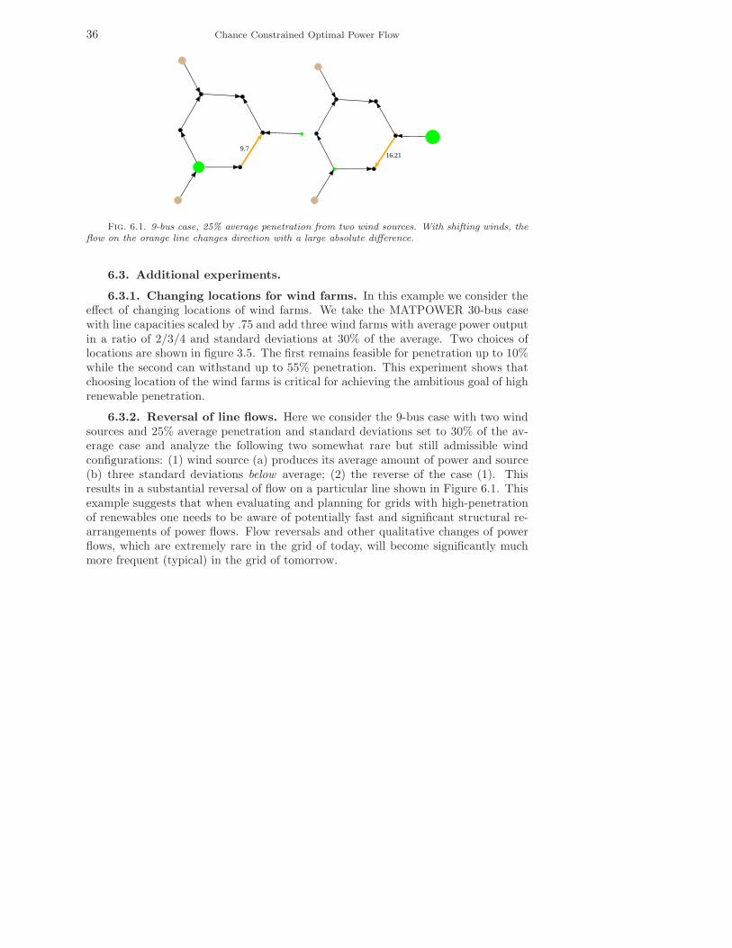
36 Chance Constrained Optimal Power Flow
9.716.21
Fig. 6.1. 9-bus case, 25% average penetration from two wind sources. With shifting winds, theflow on the orange line changes direction with a large absolute difference.
6.3. Additional experiments.
6.3.1. Changing locations for wind farms. In this example we consider theeffect of changing locations of wind farms. We take the MATPOWER 30-bus casewith line capacities scaled by .75 and add three wind farms with average power outputin a ratio of 2/3/4 and standard deviations at 30% of the average. Two choices oflocations are shown in figure 3.5. The first remains feasible for penetration up to 10%while the second can withstand up to 55% penetration. This experiment shows thatchoosing location of the wind farms is critical for achieving the ambitious goal of highrenewable penetration.
6.3.2. Reversal of line flows. Here we consider the 9-bus case with two windsources and 25% average penetration and standard deviations set to 30% of the av-erage case and analyze the following two somewhat rare but still admissible windconfigurations: (1) wind source (a) produces its average amount of power and source(b) three standard deviations below average; (2) the reverse of the case (1). Thisresults in a substantial reversal of flow on a particular line shown in Figure 6.1. Thisexample suggests that when evaluating and planning for grids with high-penetrationof renewables one needs to be aware of potentially fast and significant structural re-arrangements of power flows. Flow reversals and other qualitative changes of powerflows, which are extremely rare in the grid of today, will become significantly muchmore frequent (typical) in the grid of tomorrow.