Instrument Calibration andUncertainty Analysis

1 Calibration of an Instrument

The static performance charactertistics of an instrument can be determinedby ANSI/ISA Standard 51.1 “Process Instrumentation Terminology”. Thisstandard gives the definition for the following important characteristics:

1. Accuracy – the maximum difference between measurements and a stan-dard (or reference) as determined by testing over the range of the in-strument.

2. Repeatability – the maximum difference between repeated measure-ments of the same standard in the same direction of measurement (i.e.increasing or decreasing the input).

3. Resolution – the smallest increment you can read on the scale. If youcan see a ‘half’ increment (i.e. the space between the tick marks), thenthe resolution will be one half of the unit spacing.

4. Range – the maximum and minimum values you can measure (for ex-ample: 0 – 10 mm).

5. Span – the algebraic difference between the upper and lower rangevalues.

1

Example 1You wish to determine the accuracy and repeatability of your bathroom

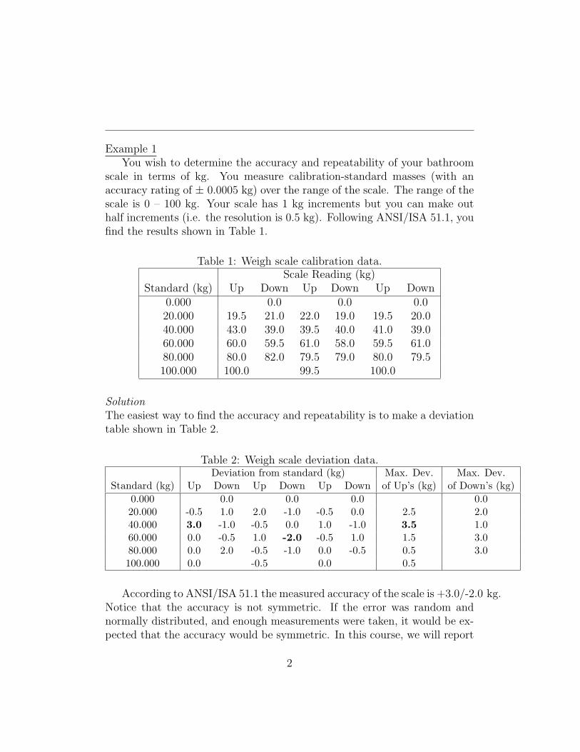
scale in terms of kg. You measure calibration-standard masses (with anaccuracy rating of ± 0.0005 kg) over the range of the scale. The range of thescale is 0 – 100 kg. Your scale has 1 kg increments but you can make outhalf increments (i.e. the resolution is 0.5 kg). Following ANSI/ISA 51.1, youfind the results shown in Table 1.

Table 1: Weigh scale calibration data.Scale Reading (kg)

Standard (kg) Up Down Up Down Up Down0.000 0.0 0.0 0.020.000 19.5 21.0 22.0 19.0 19.5 20.040.000 43.0 39.0 39.5 40.0 41.0 39.060.000 60.0 59.5 61.0 58.0 59.5 61.080.000 80.0 82.0 79.5 79.0 80.0 79.5100.000 100.0 99.5 100.0

SolutionThe easiest way to find the accuracy and repeatability is to make a deviationtable shown in Table 2.

Table 2: Weigh scale deviation data.Deviation from standard (kg) Max. Dev. Max. Dev.

Standard (kg) Up Down Up Down Up Down of Up’s (kg) of Down’s (kg)0.000 0.0 0.0 0.0 0.020.000 -0.5 1.0 2.0 -1.0 -0.5 0.0 2.5 2.040.000 3.0 -1.0 -0.5 0.0 1.0 -1.0 3.5 1.060.000 0.0 -0.5 1.0 -2.0 -0.5 1.0 1.5 3.080.000 0.0 2.0 -0.5 -1.0 0.0 -0.5 0.5 3.0100.000 0.0 -0.5 0.0 0.5

According to ANSI/ISA 51.1 the measured accuracy of the scale is +3.0/-2.0 kg.Notice that the accuracy is not symmetric. If the error was random andnormally distributed, and enough measurements were taken, it would be ex-pected that the accuracy would be symmetric. In this course, we will report

2

the accuracy symmetrically using the most conservative estimate. This wouldbe similar to the accuracy rating given by a manufacturer. This gives an ac-curacy of ±3.0 kg or ±3% “Full Scale” (or FS) or “Span”. We will state theaccuracy this way because: 1) it makes further uncertainty analysis easier,and 2) we rarely have time to repeat the experiment enough times to ensurerandom occurrences do not skew our results (typically a minimum of five upand five down traverses are used).

The repeatability is simply the maximum deviation between repeatedmeasurements of the same value approached from the same direction. In thiscase the repeatability is 3.5 kg or 3.5% of span.

Note: According to ANSI/ISA 51.1, if the accuracy rating of the standardis less than one tenth of the accuracy of the instrument tested, then theaccuracy rating (or inaccuracy) of the standard may be ignored. Since theaccuracy rating of the masses is ±0.0005 kg and the accuracy of the scale is±3.0 kg, the uncertainty in the masses is simply ignored.

2 Uncertainty in a Measurement

Let’s say you know the accuracy of an instrument and you use the instrumentto measure some property. What is the uncertainty in that measurement?This section will explain how to determine the uncertainty in an experimentalmeasurement, but first we must cover a few important definitions.

The error is defined as the difference between the true value and themeasured value. Since we can never know the true value of a property wecan NEVER know the error in the measurement. What we can do is estimatethe uncertainty in our estimate of the true value. The uncertainity is simplythe estimate of the error with a given confidence interval.

The International Standards Organization (ISO) defines two types of un-certainty:

1. Type A Uncertainty (Px) – The uncertainty estimated from the data,sometimes this is called ‘precision’ or ‘repeatability’ uncertainty. (How-ever, as we will see later, this is not the same ‘repeatability’ as definedabove in the ANSI/ISA standard. Therefore, I will try to stick to theterm ‘precision’ when discussing Type A uncertainty.)

2. Type B Uncertainty (Bx) – Uncertainties that can’t be analyzed from

3

the data and must be estimated from other sources. Sometimes this iscalled ‘systematic’ or ‘bias’ uncertainty.

The total uncertainty (Ux) in a measurement is:

Ux =√∑

B2x + P 2

x (1)

2.1 Precision Uncertainty (Px)

By taking repeated measurements of the property we are trying to determinewe will obtain a distribution of measurements. An important result fromstatistics is the central limit theorem (see Sec. 3.6 in Beckwith). Neglectingany bias error and for a large sample size, the central limit theorem states:

x− zc/2Sx√n< µ < x+ zc/2

Sx√n

(2)

where µ is the true mean value of the property, x is the mean of the mea-surements, zc/2 is the z-score of the normal distribution with c% confidence,Sx is the standard deviation of the measurements, and n is the number of

measurements taken. Therefore, the estimate of the true value is x± zc/2Sx√n

with c% confidence. The term zc/2Sx√n

is simply the precision uncertainty

(i.e. Px = zc/2Sx√n

).

If the sample size is small (n <30), the t-distribution must be used,therefore:

Px = tα2,νSx√n

(3)

where α = 1 − c, and ν = n − 1 is the degrees of freedom. Values for thet-distribution are shown in Figure 1.

Note: A confidence interval of 95% is almost universally used in calcula-tions.

2.2 Bias Uncertainty

Bias error will consistently introduce error in our measurement and since itis systematic there is no way to determine it from making repeated measure-ments. Therefore we are left to making estimates of this uncertainty (see

4

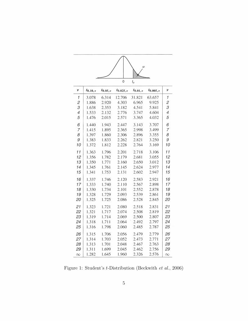
Figure 1: Student’s t-Distribution (Beckwith et al., 2006)

5

Sec. 3.9 in Beckwith). A very common estimate of the bias uncertainty isby using the manufacturer’s specification for accuracy or the accuracy deter-mined by your own calibration of an instrument. Regardless of the sourceof this estimate, it is important that the estimate of the bias uncertaintyhas the same confidence interval as the precision uncertainty. If we use theANSI/ISA 51.1 definition for accuracy we have no idea what the confidenceinterval is. However, most people assume that the accuracy rating has a95% confidence. In fact this will be a conservative estimate considering thataccuracy is defined as the maximum deviation from the standard.

Other bias errors might not be covered in the accuracy of the instrumentand must be accounted for elsewhere, such as spatial variation of the propertyor any effect the instrument might have on the system.

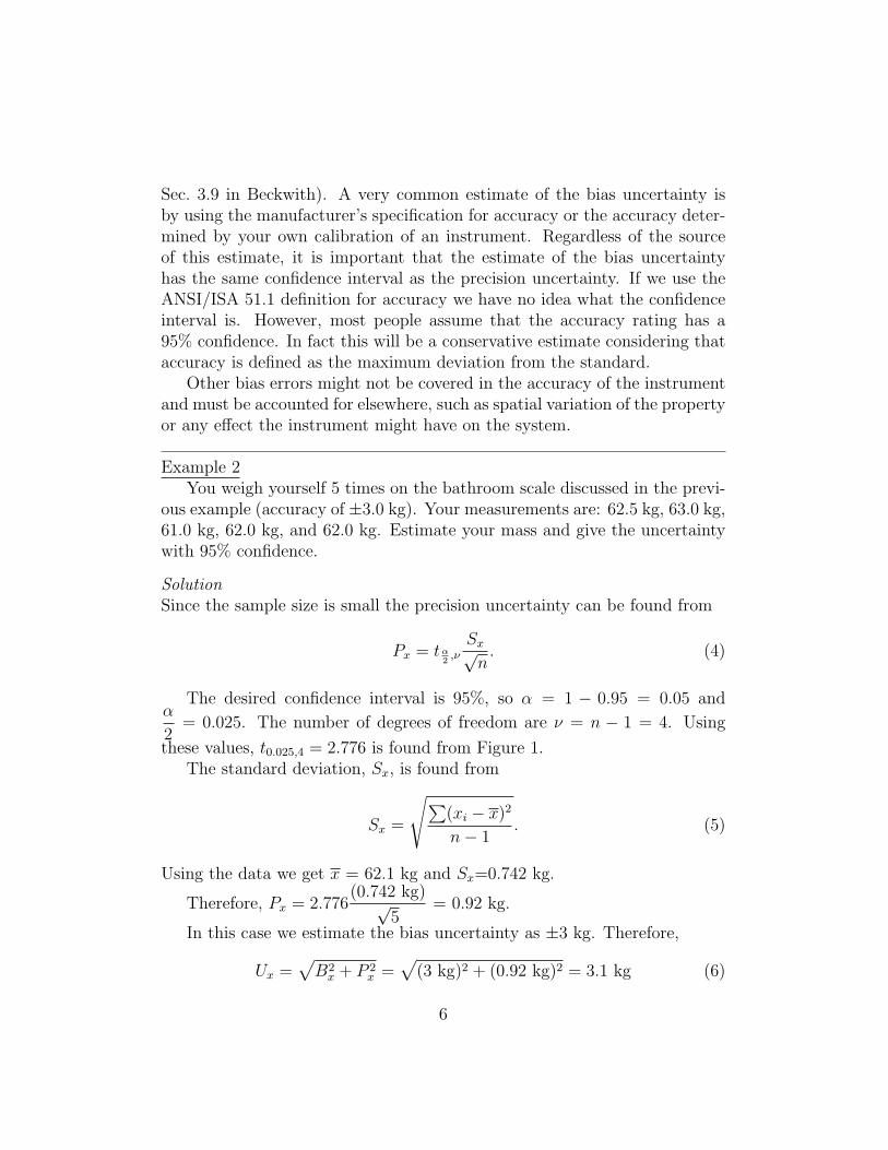
Example 2You weigh yourself 5 times on the bathroom scale discussed in the previ-

ous example (accuracy of ±3.0 kg). Your measurements are: 62.5 kg, 63.0 kg,61.0 kg, 62.0 kg, and 62.0 kg. Estimate your mass and give the uncertaintywith 95% confidence.

SolutionSince the sample size is small the precision uncertainty can be found from

Px = tα2,νSx√n. (4)

The desired confidence interval is 95%, so α = 1 − 0.95 = 0.05 andα

2= 0.025. The number of degrees of freedom are ν = n − 1 = 4. Using

these values, t0.025,4 = 2.776 is found from Figure 1.The standard deviation, Sx, is found from

Sx =

√∑(xi − x)2

n− 1. (5)

Using the data we get x = 62.1 kg and Sx=0.742 kg.

Therefore, Px = 2.776(0.742 kg)√

5= 0.92 kg.

In this case we estimate the bias uncertainty as ±3 kg. Therefore,

Ux =√B2x + P 2

x =√

(3 kg)2 + (0.92 kg)2 = 3.1 kg (6)

6

Therefore, your weight is estimated to be 62.1 ± 3.1 kg with a confidenceof 95%.

NOTE: In this case the precision uncertainty had little effect on the totaluncertainty. Therefore, less measurements could have been made withoutmuch compromise in the total uncertainty in the measurement. To make adrastic improvement in the measurement uncertainty a more accurate scalewould be required.

2.3 Single-Sample Precision Uncertainty

Ideally several measurements are taken of a property to minimize the pre-cision uncertainty. However, it may occur that only one measurement ispossible. If this is the case Eq. 3 will no longer hold because Sx and tα

2,ν are

undefined. In this case it is common to estimate the precision uncertaintyas,

Px ≈ zc/2σe ≈ 2σe, (7)

where σe is the standard deviation of measurements that were taken at someother time with the same instrument (e.g. when the instrument was cali-brated), and where the zc/2 ≈ 2 for a 95% confidence interval.

Example 3You weigh yourself once with the bathroom scale described in Example 1

and obtain a measurement of 62.5 kg. Estimate your mass and give theuncertainty with 95% confidence.

Solution

Since you have only made one measurement you must estimate the pre-cision uncertainty using the single-sample assumption. In this case you canuse the calibration data in Example 1 to find σe. The standard deviation ofall the data points in Table 2 is 1.02 kg. Therfore,

Px ≈ 2(1.02 kg) = 2.04 kg (8)

andUx =

√B2x + P 2

x =√

(3 kg)2 + (2.04 kg)2 = 3.6 kg (9)

7

Therefore, your weight is estimated to be 62.5 ± 3.6 kg with a confidenceof 95%.

3 Propagation of Uncertainty

If we know the equations that describe a system, it is possible to estimatethe probable uncertainty in a variable from the known uncertainties in othervariables. This is sometimes called an external estimate of error, because itcan be made without doing any experiments.

3.1 Analysis of Equations for Small Errors

Consider an output y that is a function of inputs x1, x2, etc. y = y(x1, x2, x3, . . . , xn)Then, take the derivative

dy =∂y

∂x1

dx1 +∂y

∂x2

dx2 + · · ·+ ∂y

∂xndxn (10)

Variation dy of y is produced by the variations dx1 etc. Interpret thesevariations as uncertainties, “ε”.

εy =∂y

∂x1

ε1 +∂y

∂x2

ε2 + · · ·+ ∂y

∂xnεn (11)

We can’t evaluate εy directly because we don’t know if the errors arepositive or negative. To get around this square both sides, and note that onaverage the cross product terms

· · ·+ ∂y

∂x1

∂y

∂x5

ε1ε5 + . . . (12)

will disappear. It can be proved that these cross products will vanish ifthe errors are symmetrically distributed random values that are statisticallyindependent of each other. Neglecting cross products leads to a simpleexpression for the mean square uncertainty

ε2y =

n∑i=1

(∂y

∂xi

)2

ε2i (13)

This result may be stated as:

8

The mean square uncertainty in a quantity y is found by addingthe mean square uncertainties of all variables contributing to y,as long as the errors are random and independent of each other.

Because ε2y and ε2

i are just the variances of each component, this is thesame as the theorem that states: “the variances of random components addto produce the function’s variance”.

3.2 Fractional Uncertainty in Purely Multiplicative Equa-tions

For equations that are purely multiplicative, the fractional or percentageuncertainty can be found without first calculating the partial derivatives inEq.13. The short cut method is as follows:

First take the natural logarithm of both sides of the equation.

Then take the derivative of both sides of the equation, notingthat for any variable xi,

d(lnxi) =dxixi

Interpret the differentials, dxi,as small uncertainties so that

dxi ≡ εi

Square both sides of the equation, discarding the cross products.(This is equivalent to simply squaring each term separately andsumming).

For example, consider the purely multiplicative equation

Q = A1FaGbHc (14)

where A1, a, b and c are constants that can be positive or negative. To findthe effect of uncertainties in F,G and H on the function Q follow the abovefour steps.

lnQ = ln(A1FaGbHc) (15)

9

Differentiate, noting A1=constant

dQ

Q= a

dF

F+ b

dG

G+ c

dH

H(16)

Interpret differentials as uncertainties and square each term to obtain(εQQ

)2

= a2(εFF

)2

+ b2(εGG

)2

+ c2(εHH

)2

(17)

Here we see the square of the fractional (or percentage) uncertainty in eachvariable is weighted by the square of its exponent.

This result is very helpful in planning an experiment. It tells us thatvariables that appear to large exponents should be measured much more ac-curately than those with small exponents. For example, if we were measuringF,G and H in an equation like

Q = A1F1/2G−3H−1/3

The percentage uncertainty in G is six times more important than uncertain-ties in F because G has an exponent of 3 and F has an exponent of 1

2.

Example 4The power P dissipated by an electrical resistor R is related to voltage

E and current I by P = EI where E = IR. If we know that the voltmeterhas an uncertainty of ±2% of reading and the resistance is known to ±1.5%,what is the percentage uncertainty in current I and in power P?

Solution

P =E2

R

ε2p =

(∂P

∂EεE

)2

+

(∂P

∂RεR

)2

ε2p =

(∂P

∂EεE

)2

+

(∂P

∂RεR

)2

= 4E2

R2ε2E +

E4

R4ε2R

Divide this equation by P 2 =E4

R2to get fractional uncertainty

10

ε2P

P 2= 4

(εEE

)2

+(εRR

)2

εPP

=√

4(0.02)2 + (0.015)2 = 0.043

which is a±4.3% probable error for power. For current, first solve E = IRfor I to make I the dependant variable.

I =E

R

ε2I =

(∂I

∂EεE

)2

+

(∂I

∂RεR

)2

=

(1

RεE

)2

+

(−ER2

εR

)2

Divide by I2 =E2

R2for fractional error(εI

I

)2

=(εEE

)2

+(εRR

)2

or (εII

)=√

(0.02)2 + (0.015)2 = 0.025

which is a 2.5% estimate of the error for current.

Alternate SolutionBecause the equations for power and current are purely multiplicative,

take ln value of both sides

P =E2

R

lnP = 2 lnE − lnR

differentiatedP

P= 2

dE

E− dR

R

Note that this equation shows that uncertainties in E are a factor of 2more important than uncertainties in R. This is because the exponent of Eis 2 in the equation for P . Interpret differentials as ε’s and square

11

(εPP

)2

=(

2εEE

)2

+(εRR

)2

(εPP

)=√

(2(0.02))2 + (0.015)2 = 0.043

Similarly, for the uncertainty in I, first solve the purely multiplicativeequation for I,

I =E

R

Then take the logarithm of both sides,

ln I = lnE − lnR

The derivation of this is

dI

I=dE

E− dR

R

Interpret dI as εI ect.(εII

)2

=(εEE

)2

+(εRR

)2

Using the given numerical values,

εII

=√

(0.02)2 + (0.015)2 = 0.025

Example 5Two electrical signals are combined, each having a random uncorrelated

RMS (root-mean-square) noise level:SIGNAL A 2.0 V with 3 mV RMS noiseSIGNAL B 6.0 V with 5 mV RMS noiseThe basic equation is E = EA + EB. What will the magnitude of the

combined signal and RMS noise be?

12

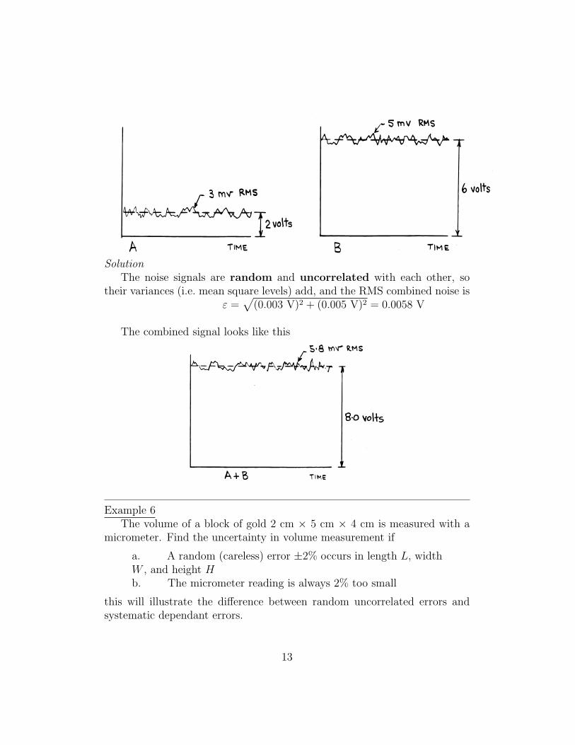
SolutionThe noise signals are random and uncorrelated with each other, so

their variances (i.e. mean square levels) add, and the RMS combined noise isε =

√(0.003 V)2 + (0.005 V)2 = 0.0058 V

The combined signal looks like this

Example 6The volume of a block of gold 2 cm × 5 cm × 4 cm is measured with a

micrometer. Find the uncertainty in volume measurement if

a. A random (careless) error ±2% occurs in length L, widthW , and height Hb. The micrometer reading is always 2% too small

this will illustrate the difference between random uncorrelated errors andsystematic dependant errors.

13

Solutiona. Volume V = LWH

ε2V =

(∂V

∂LεL

)2

+

(∂V

∂WεW

)2

+

(∂V

∂HεH

)2

= (WHεL)2 + (LHεW )2 + (LWεH)2

Divide by V 2 = (LWH)2

εVV

=

√(εLL

)+(εWW

)+(εHH

)=√

(0.02)2 + (0.02)2 + (0.02)2

= 0.035

This is 3.5% in volume

b. However if all three readings are too small by 2%, they combinesystematically

εVV

= 1.0− (0.98)3

= 1.0− 0.941

= 0.059

This is 5.9% in volume

To minimize this systematic summing effect it is best to design experimentsand connect instruments so errors remain independent of each other.

Example 7To illustrate how non-linear terms in an equation can alter the relativeimportance of errors, consider the volume flow rate Q of water over a weir.The water flows at depth H over a weir of width B.

Q = 3.33(BH3/2 − 0.2H5/2)

The constant 3.33 has the units of m1/2/s, the square root of gravitationalacceleration g.

14

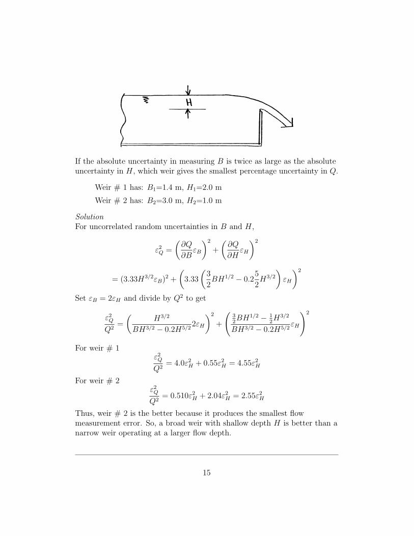
If the absolute uncertainty in measuring B is twice as large as the absoluteuncertainty in H, which weir gives the smallest percentage uncertainty in Q.

Weir # 1 has: B1=1.4 m, H1=2.0 m

Weir # 2 has: B2=3.0 m, H2=1.0 m

SolutionFor uncorrelated random uncertainties in B and H,

ε2Q =

(∂Q

∂BεB

)2

+

(∂Q

∂HεH

)2

= (3.33H3/2εB)2 +

(3.33

(3

2BH1/2 − 0.2

5

2H3/2

)εH

)2

Set εB = 2εH and divide by Q2 to get

ε2Q

Q2=

(H3/2

BH3/2 − 0.2H5/22εH

)2

+

(32BH1/2 − 1

2H3/2

BH3/2 − 0.2H5/2εH

)2

For weir # 1ε2Q

Q2= 4.0ε2

H + 0.55ε2H = 4.55ε2

H

For weir # 2ε2Q

Q2= 0.510ε2

H + 2.04ε2H = 2.55ε2

H

Thus, weir # 2 is the better because it produces the smallest flowmeasurement error. So, a broad weir with shallow depth H is better than anarrow weir operating at a larger flow depth.

15

Example 8The moment of inertia of a cylinder of radius r, length L and density ρ isgiven by

Ix =mr2

2

where the mass m = ρπr2L if the uncertainty in ρ is ±2% and theuncertainty in L is ±1%, how precisely must we measure r in order that theuncertainty in Ix is less than 5%?

SolutionCombining the two equations, the dependant variable, Ix, is

Ix =π

2ρr4L

Taking ln values of both sides of this purely multiplicative equation

ln(Ix) = lnπ

2+ ln ρ+ 4 ln r + lnL

ThendIxIx

= 0 +dρ

ρ+ 4

dr

r+dL

L

From which we can see that the uncertainty in radius r is four times asimportant as uncertainties in ρ of L.Squaring (

εIxIx

)2

=

(ερρ

)2

+ 16(εrr

)2

+(εLL

)2

(0.05)2 = (0.02)2 + 16(εrr

)2

+ (0.01)2

we findεrr

= 0.011

so the radius r must be in error no more than ±1.1%, and independent oferror in L (e.g. use a different ruler, and a different person to read it).

16