bungay castle - suffolk...

1

Bungay Castle Bungay, Suffolk Client: Olly Barnes, Bungay Castle Trust Date: September 2017 BUN 004 Geophysical Surveys Report SACIC Report No. 2017/078 Author: Timothy Schofield HND BSc MCIfA © SACIC

Bungay Castle, Bungay, Suffolk BUN 004

Geophysical Survey Report

SACIC Report No. 2017/078

Author: Timothy Schofield

Illustrator: Timothy Schofield

Editor: Stuart Boulter

Report Date: September 2017

HER Information Site Code: BUN 004

Event Number: ESF 25629

Site Name: Bungay Castle, Bungay, Suffolk

Report Number 2017/078

Planning Application No: n/a

Date of Fieldwork: July 13th – 16th Aug 2017

Grid Reference: TL 3350 8973

Oasis Reference: 289865

Curatorial Officer: Nick Carter, Will Fletcher, Historic England

Project Officer: Timothy Schofield

Client/Funding Body: Olly Barnes, Bungay Castle Trust

Client Reference: n/a

Digital report submitted to Archaeological Data Service:

http://ads.ahds.ac.uk/catalogue/library/greylit

Disclaimer Any opinions expressed in this report about the need for further archaeological work are those of Suffolk

Archaeology CIC. Ultimately the need for further work will be determined by the Local Planning Authority

and its Archaeological Advisors when a planning application is registered. Suffolk Archaeology CIC

cannot accept responsibility for inconvenience caused to the clients should the Planning Authority take a

different view to that expressed in the report.

Prepared By: Timothy Schofield

Date: September 2017

Approved By: Rhodri Gardner

Position: Director

Date: September 2017

Signed:

http://ads.ahds.ac.uk/catalogue/library/greylit

Contents Summary

1. Introduction 1

2. Geology and topography 3

3. Archaeology and historical background 4

4. Methodology 4

5. Results 8

6. Conclusion & archaeological potential 12

7. Archive deposition 13

8. Acknowledgements 13

9. Bibliography 14

List of Figures

Figure 1. Location map 2 Figure 2. Survey area (red) and grid location (purple) in relation to the Scheduled Monument (blue) 3 Figure 3. Survey grid, GPR traverses & georeferencing information 15 Figure 4. Raw magnetometer greyscale plot 16 Figure 5. Processed magnetometer greyscale plot 17 Figure 6. Processed magnetometer xy trace plot 18 Figure 7. Interpretation plot of magnetometer anomalies 19 Figure 8. Raw earth resistance meter greyscale plot 20 Figure 9. Processed earth resistance meter greyscale plot 21 Figure 10. Processed earth resistance meter xy trace plot 22 Figure 11. Interpretation plot of earth resistance meter anomalies 23 Figure 12. Processed GPR timeslice greyscale plots 24 Figure 13. Interpretation plot of GPR anomalies 25 Figure 14. Combined interpretation plot of geophysical survey anomalies 26

List of Appendices

Appendix 1. Metadata sheets Appendix 2. Technical data Appendix 3. OASIS form

Summary In July and August 2017 Suffolk Archaeology Community Interest Company (SACIC)

undertook detailed geophysical surveys within the bailey of Bungay Castle, Bungay,

Suffolk. Three techniques were requested by Historic England to be deployed over the

0.24hectare grass covered bailey, comprising fluxgate gradiometer, earth resistance

meter and ground penetrating radar surveys.

The three instruments highlighted a narrow range of geophysical anomalies that have

significant archaeological potential, including in-situ structural remains that may include

walls, floors and a potential well. Anomalies indicative of robbed-out or service trench

runs, rubbish pits or geological deposits, demolition or levelling deposits and an extant

Tarmacadam drive were further prospected.

1

1. Introduction In July and August 2017, detailed geophysical surveys covering an area of 0.24

hectares within the bailey of the scheduled monument of Bungay Castle (National

Heritage List for England Ref. 1006060), Bungay, Suffolk (Fig.1) were undertaken by

Suffolk Archaeology Community Interest Company (SACIC).

The detailed geophysical surveys were requested by Historic England, to identify areas

of high archaeological potential. Suffolk Archaeology CIC were commissioned to

undertake the project by Olly Barnes of the Bungay Castle Trust.

2

N

Contains Ordnance Survey data © Crown copyright and database right 2017

Figure 1. Location map

3

2. Geology and topography The geophysical survey area lies within the bailey of the Scheduled Monument of

Bungay Castle (National Heritage List for England Ref. 1006060). The survey was

undertaken at the request of Nick Carter and Will Fletcher of Historic England, who

provided the Section 42 Licence.

Superficial geology is described as sand and gravel river terrace deposits, overlying a

sedimentary bedrock of Crag Group sands (British Geological Survey, 2017). The site

is broadly flat and is located at a height of c. 10m above Ordnance Datum.

Crown Copyright. All rights reserved. Licence Number: 100019980

Figure 2. Survey area (red) and grid location (purple) in relation to the Scheduled Monument (blue)

4

3. Archaeology and historical background Bungay Castle was originally built in 1100 by Roger Bigod, a Norman invader who

assisted King William in conquering England in 1066, he was rewarded for his loyalty by

being given a large area of East Anglia. In around 1165, his second son Hugh Bigod

added a stone keep that had 5 - 7m thick walls and stood to a height of 33m. This

version of the castle was destroyed in 1174 during a revolt. Hugh Bigod died in 1178

and the castle remained uninhabited until 1269, when Roger Bigod inherited the title,

built the gate towers and renovated the castle, he died shortly after the castle was

completed in 1297 and the castle fell into disrepair.

In 1934 Dr Leonard Cane started a programme of excavation and repair, revealing

many features that were hidden. The Duke of Norfolk presented the castle to the town

in 1987 with an endowment to help towards its preservation; today it is owned and

administered by the Bungay Castle Trust.

A geophysical survey employing an earth resistance meter and a fluxgate gradiometer

was undertaken on the bailey by Geophysical Surveys of Bradford in 1990 (Gaffney and

Gater, 1990). Subtle anomalies were noted by the authors that included a wall and

made ground layers; however, their archaeological significance could not be

determined.

4. Methodology

Instrument types Three different instruments were used to undertake the geophysical survey. A

Bartington DualGrad 601-2 fluxgate gradiometer, a Geoscan Research RM85 advanced

earth resistance meter and an Utsi Electronics TriVue ground penetrating radar. The

weather for the magnetometer survey was sunny, however during the radar and

resistance meter surveys there were large downpours causing a degree of moist soil

conditions, despite this inclement weather the ground conditions were found to be

suitable.

Survey grid layout The detailed fluxgate gradiometer and earth resistance meter surveys were undertaken

5

on the same 20m grid (Fig. 3, blue grid), orientated east to west and geolocated

employing a Leica Viva GS08+ Smart Rover RTK GLONASS/GPS, allowing an

accuracy of +/- 0.03m. Data were converted to National Grid Transformation OSTN15.

The ground penetrating radar survey was undertaken along traverses that are also

illustrated in Figure 3 (cyan lines).

Survey grid restoration Three virtual survey grid stations were placed on survey grid nodes along the baselines

of the survey grid, this will allow both the grid and the anomalies to be accurately

relocated (Fig. 3).

Bartington DualGrad 601-2

The first instrument to be deployed over the bailey was the Bartington DualGrad 601-2,

the magnetic background was found to be very high during the initial site scan, therefore

it was decided to calibrate the instrument in the meadow further down slope from the

survey area.

Instrument calibration and settings

One hour was allocated to allow the instruments’ sensors to reach optimum operating

temperature before the survey commenced. Instrument sampling intervals were set to

0.125m along 1m traverses (eight readings per metre).

Data capture

Detailed fluxgate gradiometer survey data points were recorded on an internal data

logger that were downloaded and checked for quality at midday and in the evening,

allowing grids to be re-surveyed if necessary. A pro-forma survey sheet was completed

to allow data composites to be created. Data were filed in unique project folders and

backed-up onto an external storage device and then a remote server in the evening.

Data software, processing and presentation

The site had a high magnetic signature, however the strong anomalies contrasted well

6

with this increased magnetic background allowing good quality raw survey data to be

collected, which required minimal data processing. Datasets were composited and

processed using DW Consulting’s Terrasurveyor v.3.0.32.4; raw grid files, composites

and raster graphic plots will be stored and archived in this format. Minimal processing

algorithms were undertaken on the raw (Fig. 4 and processed datasets (Figs. 5 - 6);

schedules are presented in Appendix 1.

Data composites were exported as raster images into AutoCAD. An interpretation plan

based on the combined results of the raw, processed and xy trace plots (Figs. 4 - 6) has

been produced (Fig. 7).

Geoscan Research RM85 Advanced

The earth resistance meter survey was undertaken along the same grid as the fluxgate

gradiometer survey with only the Tarmacadam road being unsuitable for survey.

Sampling intervals were set to 0.5m along 0.5m traverses.


A three-parallel twin (six probe pole-pole) array was employed, gain was set to 10,

frequency was 122.5Hz with an output voltage of 45v, the auto-log delay was 300ms

and the high-pass filter was 0hz. Station readings were equalised when the remote

probes were moved to allow consistent data matching between the survey grids.

Data capture

Detailed earth resistance meter data points were recorded on an internal data logger

that were downloaded and checked for quality at midday and in the evening, allowing

grids to be re-surveyed if required. A pro-forma survey sheet was completed to allow

data composites to be created. Data were filed in unique project folders and backed-up

onto an external storage device and then a remote server in the evening.


The ground conditions for the earth resistance meter were found to be good, the level of

precipitation allowed the electrical current to pass through the sandy soil with relative

7

ease. Good quality raw survey data was therefore collected requiring minimal data

processing. Datasets were composited and processed using DW Consulting’s

Terrasurveyor v.3.0.32.4; raw grid files, composites and raster graphic plots will be

stored and archived in this format. Minimal processing algorithms were undertaken on

the raw (Fig. 8) and processed datasets (Figs. 9 - 10); schedules are presented in

Appendix 1.

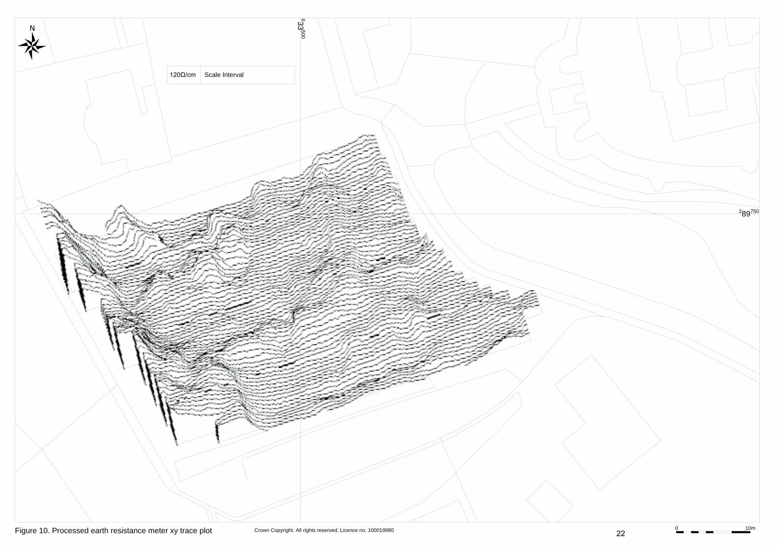
Data composites were exported as raster images into AutoCAD. An interpretation plan

based on the combined results of the raw, processed and xy trace plots (Figs. 8 – 10)

has been produced (Fig. 11).

UTSI TriVue multi-frequency ground penetrating radar

The ground penetrating radar (GPR) survey was undertaken along survey traverses that

were 0.50m apart, readings were taken at 0.05m intervals along the traverse. Ground

water issues were a concern on site with downpours occurring before and during the

survey, however the free draining nature of the sandy geology helped to disperse the

rainwater, allowing the conditions overall to be suitable for GPR survey.


The TriVue contains three antennas of 250MHz, 500MHz and 1GHz central frequency

within the casing, which allows the operator optimum flexibility when surveying. This

antenna casing is strapped to a four-wheeled cart, allowing traverses to be recorded

with relative ease, all three antennas were operated in unison, each of their recording

lengths were independently adjusted giving the operator optimum control over antenna

depths whilst allowing quality control measures to be implemented in the field.

Data capture

Ground penetrating radar survey points were recorded on a tablet linked to an odometer

trigger, data were recorded and checked for quality during the survey, and further

composited in the evenings, which allowed traverses to be re-surveyed if required. The

data recorded by all three antennas was recorded and processed, the 500MHz antenna

was found to be most suitable over this geology. A proforma survey sheet was created

8

to allow the traverse composite to be constructed. Data were filed in unique project

folders and backed up onto an external storage device and then a remote server in the

evening.


The ground conditions for the GPR were found to be suitable, allowing good quality data

to be recorded. Individual traverses were processed using ReflexW 2D, a 3D cube was

then created utilising ReflexW 3D, which enabled the production of timeslice data. The

geometry file, raw files, processed files, cube files, timeslices and .mpg files will be

stored and archived in this format. Processing algorithm schedules are presented in

Appendix 1.

Timeslice data was exported out of ReflexW, into Terrasurveyor as raster images, these

images were then imported into AutoCAD. An interpretation plan based on the

combined timeslice results (Fig. 12) has been produced (Fig. 13).

5. Results The three geophysical survey instruments will be discussed within their separate

headings below, further comparisons will be discussed where anomalies strongly

correlate between instruments (Fig. 14).

Fluxgate gradiometer survey (Fig’s 4 - 7) The site conditions for the fluxgate gradiometer survey were the most challenging of the

three techniques employed, predominantly due to the increased magnetic background

encountered within the bailey. A zero point was located in meadowland away from the

site that allowed the sensors to be successfully calibrated. Despite the ‘noisy’ magnetic

signature of the survey area a range of anomalies were recorded that have a high

degree of archaeological potential.

A corner of two adjoining linear anomalies of magnetic disturbance (red hatching),

orientated north-northwest to south-southeast and perpendicular were recorded in the

dataset running along the southern boundary of the survey area and to the west of the

9

Tarmacadam drive (dark blue hatching). These anomalies are similar to those caused

by services, however both appear to terminate within the survey area and are therefore

more likely to be of a structural derivation. Low resistance and intermittent high

resistance anomalies recorded by the earth resistance meter in the same location (Fig’s

8 - 11) indicate that these structures may have been partially robbed-out to reclaim

building materials for reuse sometime in the past.

One irregular area of magnetic disturbance (cyan hatching) located in the northeastern

corner of the dataset is indicative of a dump of building material, or potentially a building

platform. The ground penetrating radar survey recorded an area of high amplitude and

the earth resistance meter prospected a high resistance linear anomaly in this same

location, together this provides evidence for an anomaly of good archaeological

potential.

An oval area of magnetic disturbance (magenta hatching) prospected in the southern

half of the survey area is likely to record the location of a well-type structure, the

readings are strongly magnetic and may indicate that it was built of brick. In this same

location, the earth resistance meter records a blank area within structural remains and

the GPR survey prospected an oval high amplitude response.

Areas of magnetic disturbance (green hatching) located on the periphery of the survey

area record the presence of ferrous fences and benches positioned around the edge of

the bailey.

Isolated dipolar anomalies (grey spots) were recorded within the dataset that are

indicative of ferrous rubbish deposited within the bailey. It is possible that some of

these responses are caused by ferrous archaeological finds or equally could derive from

modern debris.

Earth resistance meter survey (Fig’s 8 - 11) The earth resistance meter survey was successful in recording a fairly narrow range of

geophysical anomalies, some of which correlate well with anomalies prospected by both

the magnetometer and GPR instruments.

10

High resistance linear anomalies (red hatching) were recorded in two orientations, the

first being north-northeast to south-southwest and perpendicular and the second west-

northwest to south-southeast and perpendicular. These responses are likely to be

caused by building construction and may prove to be walls or foundations that belong to

two separate phases of building activity. These results favourably correspond with

linear anomalies recorded during both the magnetometer and GPR surveys and

strongly suggest that the remains of buildings are still present below the ground surface

of the castle’s bailey.

Two areas of high resistance (magenta hatching) were recorded on the western and

eastern periphery of the survey area, the deposits here are likely to be made up of

moisture poor compacted materials. The larger high resistance anomaly located to the

west is interpreted as an area of made ground used to level the surface of the bailey. It

is possible that this material could derive from the demolition rubble of the structures

recorded to the east. The smaller area of high resistance recorded in the southeastern

corner of the dataset is of unknown origin.

Five linear areas of low resistance (dark blue hatching) record areas of moisture rich

material within the dataset. The longest of which correlates well with the linear area of

magnetic disturbance recorded by the fluxgate gradiometer (Fig. 7). The low resistance

readings recorded indicate that no compacted materials are present here, therefore the

anomaly is more likely to be a service trench or a robbed-out wall foundation trench.

Eleven discrete low resistance anomalies (cyan hatching) were prospected, many of

which are located close to the anomalies indicative of structural remains. The character

of this material indicates that it has a high moisture content and is therefore likely to be

saturated material abutting the walls or naturally occurring geological variations.

Ground penetrating radar survey (Fig’s 12 - 13) The ground penetrating radar performed favourably over the survey area, recording

anomalies of high archaeological potential. Its results correlate with those recorded by

the other two techniques, confirming the presence of anomalies in some areas and

increasing the detail of anomalies recorded (particularly those of a structural nature).

11

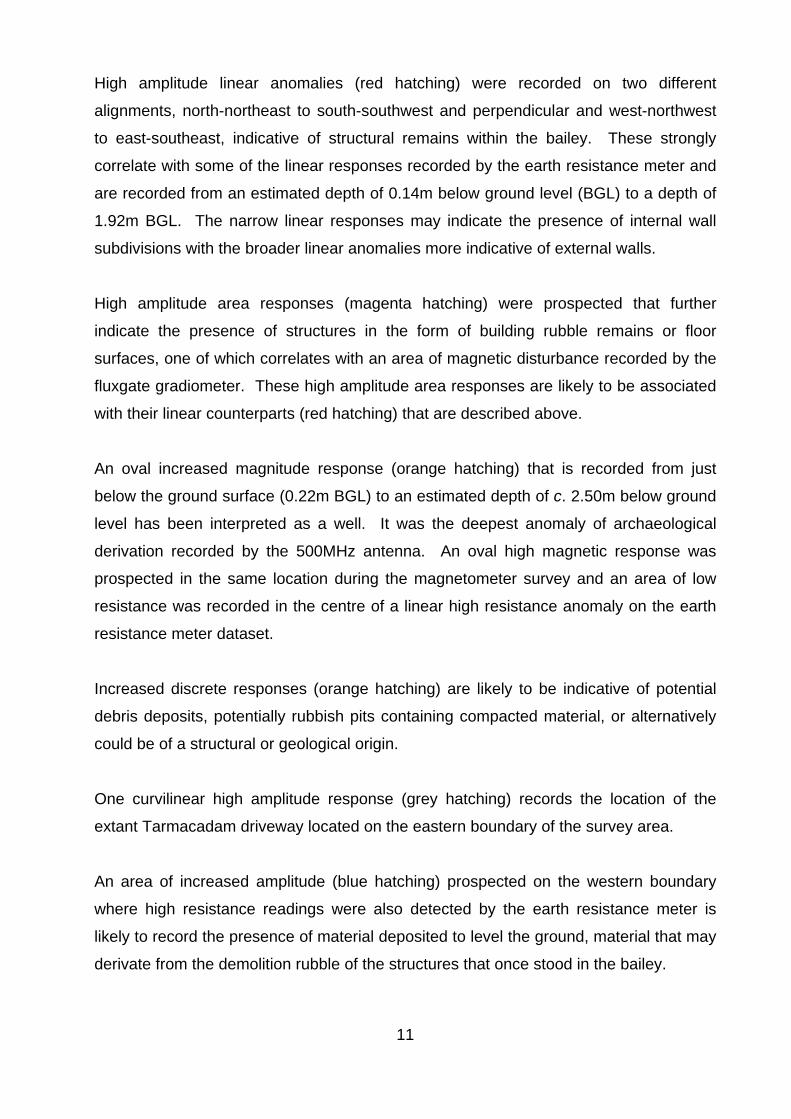
High amplitude linear anomalies (red hatching) were recorded on two different

alignments, north-northeast to south-southwest and perpendicular and west-northwest

to east-southeast, indicative of structural remains within the bailey. These strongly

correlate with some of the linear responses recorded by the earth resistance meter and

are recorded from an estimated depth of 0.14m below ground level (BGL) to a depth of

1.92m BGL. The narrow linear responses may indicate the presence of internal wall

subdivisions with the broader linear anomalies more indicative of external walls.

High amplitude area responses (magenta hatching) were prospected that further

indicate the presence of structures in the form of building rubble remains or floor

surfaces, one of which correlates with an area of magnetic disturbance recorded by the

fluxgate gradiometer. These high amplitude area responses are likely to be associated

with their linear counterparts (red hatching) that are described above.

An oval increased magnitude response (orange hatching) that is recorded from just

below the ground surface (0.22m BGL) to an estimated depth of c. 2.50m below ground

level has been interpreted as a well. It was the deepest anomaly of archaeological

derivation recorded by the 500MHz antenna. An oval high magnetic response was

prospected in the same location during the magnetometer survey and an area of low

resistance was recorded in the centre of a linear high resistance anomaly on the earth

resistance meter dataset.

Increased discrete responses (orange hatching) are likely to be indicative of potential

debris deposits, potentially rubbish pits containing compacted material, or alternatively

could be of a structural or geological origin.

One curvilinear high amplitude response (grey hatching) records the location of the

extant Tarmacadam driveway located on the eastern boundary of the survey area.

An area of increased amplitude (blue hatching) prospected on the western boundary

where high resistance readings were also detected by the earth resistance meter is

likely to record the presence of material deposited to level the ground, material that may

derivate from the demolition rubble of the structures that once stood in the bailey.

12

6. Conclusion & archaeological potential Figure 14 draws together the combined interpretations of all three instruments,

highlighting those anomalies that have significant archaeological potential. The

anomalies fall within five types: in-situ structural remains, robbed-out/service trench

runs, rubbish pits, demolition/levelling deposits, and extant modern furniture anomalies.

In-situ building structure remains (red hatching) are recorded on two different

orientations indicating that there could be at least two different building phases present

below the surface of the bailey at a depth ranging from c. 0.14 to 1.92m BGL.

Examples of both broad and narrow linear anomalies were recorded that are potentially

indicative of internal wall subdivisions and external wall remains. Associated with the

walls are remnant structural remains (magenta hatching) that are likely to consist of

highly compacted deposits, potentially demolition rubble from the former standing

structures and/or floor surfaces. An oval response (orange hatching) prospected by

both the magnetometer and GPR instruments has been interpreted as a brick-lined well,

recorded from c. 0.22m to approximately 2.50m below the ground surface.

Linear trench backfill anomalies (cyan hatching) may derive from robbed-out wall or

foundation trenches, however they could be indicative of service trench runs.

Two discrete moisture rich anomalies (dark blue hatching) recorded just to the

southeast of the well are potentially indicative of rubbish pits associated with the

building structures, a geological origin also cannot be ruled out.

Demolition and/or levelling deposits (green hatching) recorded by the GPR and earth

resistance meter surveys may derive from rubble associated with the demolished

building structures, or made ground material used to level the surface of the bailey.

The extant Tarmacadam drive (black hatching) is further depicted in Figure 14.

This programme of geophysical survey has for the first time provided strong evidence

that structural remains are present below the ground surface within the bailey at Bungay

Castle. The three instruments have proven to favourably complement each other with

each technique providing information that has helped to better identify the nature and

13

type of anomalies that were recorded.

7. Archive deposition The paper and digital archive will be kept at the SACIC office in Needham Market,

before deposition in the Suffolk County Council Stores in Bury St Edmunds.

8. Acknowledgements The fieldwork was carried out by Tim Schofield, Cameron Bate and Ed Palka and was

directed by Tim Schofield. Project management was undertaken by Rhodri Gardner.

The report illustrations were created by Tim Schofield and the report was edited by

Stuart Boulter.

14

9. Bibliography Ayala, G., et al, 2004, Geoarchaeology; Using Earth Sciences to Understand the

Archaeological Record. English Heritage. Brown, N., and Glazebrook, J, (eds), 2000, Research and Archaeology: A Framework

for the Eastern Counties, 2. Research Agenda and Strategy. East Anglian Archaeology Occasional Paper No. 8.

Chartered Institute for Archaeologists, 2014, Standard and Guidance for Archaeological Geophysical Survey.

Clark, A. J., 1996, Seeing Beneath the Soil, Prospecting Methods in Archaeology. BT Batsford Ltd. London.

David, A., et al, 2014, Geophysical Survey in Archaeological Field Evaluation. Historic England.

Gaffney, C., Gater. J., and Ovenden, S., 2002, The Use of Geophysical Techniques in Archaeological Evaluations. IFA Technical Paper No.6.

Gaffney, C., and Gater. J., 2003, Revealing the Buried Past, Geophysics for Archaeologists. Tempus Publishing Ltd.

Gaffney, C., and Gater. J., 1990, Report on Geophysical Survey, Bungay Castle. Geophysical Surveys Bradford, Report 90/60.

Historic England, 2015, Management of Research in the Historic Environment (MoRPHE).

Gurney, D., 2003, Standards for Field Archaeology in the East of England. East Anglian Archaeology Occasional Paper 14.

Medlycott, M. (ed), 2011, Research and Archaeology Revisited: A revised framework for the East of England. East Anglian Archaeology Occasional Paper 24.

Schmidt, A., 2001, Geophysical Data in Archaeology: A Guide to good Practice. Archaeology Data Service. Oxbow books.

Schmidt, A., et al, 2015, EAC Guidelines for the use of Geophysics in Archaeology; Questions to ask and Points to Consider. EAC Guidelines 2.

SCCAS, 2010, Deposition of Archaeological Archives in Suffolk. SCCAS, 2011, Requirements for a Geophysical Survey. Witten, A. J., 2006, Handbook of Geophysics and Archaeology. Equinox Publishing Ltd.

London. Websites British Geological Survey, 2017, http://mapapps.bgs.ac.uk/geologyofbritain/home.html

http://mapapps.bgs.ac.uk/geologyofbritain/home.html

0

1

0

2

0

3

0

5

0

4

0

6

STN 01

STN 02

STN 03

2 750

89

6 5

00

33

N

Crown Copyright. All rights reserved. Licence no. 100019980

Figure 3. Survey grid (dark blue), GPR traverses (cyan) & georeferencing information (magenta)


0 10m

Survey

Station

Easting Northing

STN 01 633465.394 289749.086

STN 02633522.395 289767.815

STN 03633528.639 289748.814

15

2 750

89

6 5

00

33

-30nT

+30nT

N


Figure 4. Raw magnetometer greyscale plot


0 10m16

2 750

89

6 5

00

33

-30nT

+30nT

N


Figure 5. Processed magnetometer greyscale plot


0 10m17

2 750

89

6 5

00

33

Scale Interval90nT/cm

N


Figure 6. Processed magnetometer xy trace plot


0 10m18

2 750

89

6 5

00

33N


Figure 7. Interpretation plot of magnetometer anomalies


Curvlinear magnetic

disturbance, Tarmacadam road

Discrete magnetic

disturbance, burnt pit?

0 10m

Magnetic disturbance, well

Magnetic disturbance, wall

foundations?

Isolated dipolar, ferrous spike

Magnetic disturbance, ferrous

boundary furniture

19

2 750

89

6 5

00

33

+65 Ω

+451 Ω

N


Figure 8. Raw earth resistance meter greyscale plot

0 10m20

2 750

89

6 5

00

33

+66Ω

+321 Ω

N


Figure 9. Processed earth resistance meter greyscale plot

0 10m21

2 750

89

6 5

00

33

Scale Interval120Ω/cm

N


Figure 10. Processed earth resistance meter xy trace plot

0 10m

22

2 750

89

6 5

00

33N


Figure 11. Interpretation plot of earth resistance meter anomalies

Low resistance linear, trench

backfill

High resistance linear, walls?

Low resistance discrete, pits?

0 10m

High resistance area

23

2 750

89

6 5

00

33N


Figure 12. Processed GPR timeslice greyscale plots


0.22m BGL

0.30m BGL

-2048mHz

+2048mHz

-2048mHz

+2048mHz

-2048mHz

+2048mHz

0 20m

-2048mHz

+2048mHz

-2048mHz

+2048mHz

-2048mHz

+2048mHz

-2048mHz

+2048mHz

-2048mHz

+2048mHz

-2048mHz

+2048mHz

0.26m BGL

0.37m BGL

0.53m BGL

0.76m BGL

0.90m BGL

1.60m BGL

1.74m BGL

2 750

89

6 5

00

33

6 5

00

33

2 750

89

2 750

89

2 750

89

6 5

00

33

6 5

00

33

6 5

00

33

6 5

00

33

6 5

00

33

6 5

00

33

24

2 750

89

6 5

00

33N


Figure 13. Interpretation plot of GPR anomalies


High amplitude, modern

Tarmacadam road

Increased amplitude, backfill

deposit

Oval, increased response,

remains of well

High amplitude linear, structural

remains

0 10m

High amplitude area, structural

remains

Increased response, discrete,

archaeology?

25

2 750

89

6 5

00

33N


Figure 14. Combined interpretation plot of geophysical survey anomalies


Tarmacadam road, high

amplitude curvilinear response

Levelling / demolition layer,

increased amplitude

Moisture rich loose material,

low amplitude response, pits?

In-situ structural remains, high

amplitude linear responses

0 10m

Remnant structural remains,

high amplitude area responses

Trench backfill, service /

robbed-out structure trench

In-situ well structure,

high amplitude oval response

26

Appendix 1. Metadata sheets

Fluxgate Gradiometer Survey Grids Source Grids: 6 1 Col:0 Row:0 grids\01.xgd 2 Col:0 Row:1 grids\02.xgd 3 Col:1 Row:0 grids\03.xgd 4 Col:1 Row:1 grids\04.xgd 5 Col:2 Row:0 grids\05.xgd 6 Col:2 Row:1 grids\06.xgd

Raw DataFilename Bungay Mag Raw.xcp Description Instrument Type Grad 601 (Gradiometer) Units nT Direction of 1st Traverse 90 deg Collection Method ZigZag Sensors 2 @ 1.00 m spacing. Dummy Value 2047.5 Dimensions Composite Size (readings) 240 x 40 Survey Size (meters) 60 m x 40 m Grid Size 20 m x 20 m X Interval 0.25 m Y Interval 1 m Stats Max 100.00 Min -100.00Std Dev 42.18 Mean -7.50Median -6.70Composite Area 0.24 ha Surveyed Area 0.1608 ha Program Name TerraSurveyor Version 3.0.32.4

Processes

Display Clip -30 +30

Graduated Shade

Processed Data Filename Bungay Mag Pro.xcp Description Instrument Type Grad 601 (Gradiometer) Units nT Direction of 1st Traverse 90 deg Collection Method ZigZag Sensors 2 @ 1.00 m spacing. Dummy Value 2047.5 Dimensions Composite Size (readings) 240 x 40 Survey Size (meters) 60 m x 40 m Grid Size 20 m x 20 m X Interval 0.25 m Y Interval 1 m Stats Max 129.96 Min -96.62 Std Dev 41.70 Mean 1.06 Median 0.00 Composite Area 0.24 ha Surveyed Area 0.1608 ha Program Name TerraSurveyor Version 3.0.32.4

Processes

Display Clip -30 +30

Graduated Shade

Destripe Median Sensors; All

Earth Resistance Meter Survey Grids Source Grids: 6 1 Col:0 Row:0 grids\01.xgd 2 Col:0 Row:1 grids\02.xgd 3 Col:1 Row:0 grids\03.xgd 4 Col:1 Row:1 grids\04.xgd 5 Col:2 Row:0 grids\05.xgd 6 Col:2 Row:1 grids\06.xgd

Raw Data

Filename Bun Res Raw.xcp Description Instrument Type GeoScan (Resistance) Units Ohm Direction of 1st Traverse 0 deg Collection Method ZigZag Sensors 1 Dummy Value 2047.5 Dimensions Composite Size (readings) 120 x 120 Survey Size (meters) 60 m x 60 m Grid Size 20 m x 30 m X Interval 0.5 m Y Interval 0.5 m Stats Max 451.00 Min 65.00 Std Dev 51.88 Mean 167.25 Median 158.00 Composite Area 0.36 ha Surveyed Area 0.15233 ha Program Name TerraSurveyor Version 3.0.32.4

Processes

n/a

Processed Data

Filename Bun Res Pro.xcp Description Instrument Type GeoScan (Resistance) Units Ohm Direction of 1st Traverse 0 deg Collection Method ZigZag Sensors 1 Dummy Value 2047.5 Dimensions Composite Size (readings) 120 x 120 Survey Size (meters) 60 m x 60 m Grid Size 20 m x 30 m X Interval 0.5 m Y Interval 0.5 m Stats Max 451.00 Min 66.00 Std Dev 51.24 Mean 166.98 Median 158.00 Composite Area 0.36 ha Surveyed Area 0.15233 ha Program Name TerraSurveyor Version 3.0.32.4

Processes

Despike, threshold 0.5m, window size 3 x 3, centre value median, replace with median

Display Clip +/-3SD (+66 / +321)

Graduated Shade

Ground Penetrating Radar Survey Traverses: 64

20170808_100_ch2

20170808_101_ch2

20170808_103_ch2

20170808_104_ch2

20170808_105_ch2

20170808_106_ch2

20170808_107_ch2

20170808_108_ch2

20170808_109_ch2

20170808_110_ch2

20170808_111_ch2

20170808_112_ch2

20170808_113_ch2

20170808_114_ch2

20170808_115_ch2

20170808_116_ch2

20170808_117_ch2

20170808_118_ch2

20170808_119_ch2

20170808_120_ch2

20170808_121_ch2

20170808_122_ch2

20170808_123_ch2

20170808_124_ch2

20170808_125_ch2

20170808_126_ch2

20170808_127_ch2

20170808_128_ch2

20170808_129_ch2

20170808_130_ch2

20170808_131_ch2

20170808_132_ch2

20170808_133_ch2

20170808_134_ch2

20170808_135_ch2

20170808_136_ch2

20170808_137_ch2

20170808_138_ch2

20170808_139_ch2

20170808_140_ch2

20170808_141_ch2

20170808_142_ch2

20170808_143_ch2

20170808_144_ch2

20170808_145_ch2

20170808_146_ch2

20170808_147_ch2

20170808_148_ch2

20170808_149_ch2

20170808_150_ch2

20170808_151_ch2

20170808_152_ch2

20170808_153_ch2

20170808_154_ch2

20170808_155_ch2

20170808_156_ch2

20170808_157_ch2

20170808_158_ch2

20170808_159_ch2

20170808_160_ch2

20170808_161_ch2

20170808_162_ch2

20170808_163_ch2

Processed Data Description

Instrument Type Surfer ASCII

Units MHz

Direction of 1st Traverse 0 deg

Collection Method ZigZag

Sensors 1 x 500MHz

Dummy Value 2047.5

Dimensions

Composite Size (readings) 1276 x 63

Survey Size (meters) 51 m x 31.5 m

Grid Size 51 m x 31.5 m

X Interval 0.04 m

Y Interval 0.5 m

Stats

Max 5624.00

Min -3178.00

Std Dev 473.26

Mean 0.29

Median 0.00

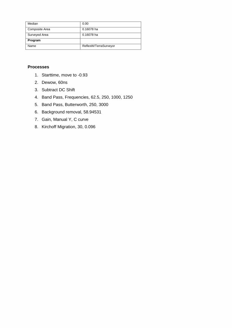
Composite Area 0.16078 ha

Surveyed Area 0.16078 ha

Program

Name ReflexW/TerraSurveyor

Processes

1. Starttime, move to -0.93

2. Dewow, 60ns

3. Subtract DC Shift

4. Band Pass, Frequencies, 62.5, 250, 1000, 1250

5. Band Pass, Butterworth, 250, 3000

6. Background removal, 58.94531

7. Gain, Manual Y, C curve

8. Kirchoff Migration, 30, 0.096

Appendix 2. Technical data Detailed magnetometer survey Detailed magnetometer survey is the most commonly employed archaeological

geophysical prospection method in Britain; sensitive sensors can cost-effectively cover

large areas of ground, rapidly recording anomalies that are indicative of cultural

settlement activity. These anomalies can then be further investigated by field

archaeologists to quantify a form and function. The magnetometer is a passive

instrument that detects both permanent thermoremanent and temporary magnetic

responses.

Thermoremanent magnetism When a material containing iron oxides, for example clay, is heated above the Curie

point, weakly magnetic compounds transform in to highly magnetic oxides that can be

detected by the sensors of a magnetometer (Clark, 1996). For instance, the iron oxide

haematite has a Curie temperature of 675 Celsius and magnetite 565 Celsius. Once

these temperatures are reached, the oxides become demagnetised, on cooling their

magnetic properties become permanently re-magnetised and align in the direction of the

Earth’s magnetic field (Gaffney and Gater, 2003). Over time the direction of the Earth’s

magnetic field changes allowing these directional differences to be detected by the

magnetometer.

Strongly heated features such as hearths, kilns or furnaces frequently reach the Curie

temperature and become permanently magnetised. These permanent magnetic

responses are some of the strongest cultural features that can be recorded.

Temporary magnetism Magnetic susceptibility is the ease with which a magnetic field can pass through a

material, therefore the higher the material’s magnetic susceptibility, the stronger the

induced magnetic field will be. Temporary magnetisation occurs within material that is

magnetically susceptible, this material acquires its own local magnetic field that

combines with the Earth’s magnetic field causing an anomaly to stand out from the

background noise (Clark, 1996). These anomalies are subtler in nature, being derived

from material that has been magnetically enhanced by cultural activity which has

become concentrated into features over time. Anomalies that have temporary

magnetisation include backfilled pits, ditches, field systems, occupation areas, land

drains, remnant and existing field boundaries (David et al, 2014).

The key to a successful survey is having good contrast between the magnetic

susceptibility of an archaeological feature with the surrounding superficial deposits. If

there is no discernible difference between the two mediums it may be unlikely that the

magnetometer will successfully prospect the feature. Archaeological features can also

be masked by high magnetically susceptible topsoil, or deep overlying subsoil and

colluvial deposits.

Ferrous anomalies Ferrous objects are a common source of permanent magnetism, usually isolated with a

strong dipolar signature. Some of these responses may have an archaeological

derivation, however they are probably more indicative of modern iron objects introduced

through manuring or lost within the topsoil.

Bartington DualGRAD 601-2 fluxgate gradiometers Fluxgate gradiometers are the most commonly employed class of instrument in the UK.

Two 1m sensitive sensors are affixed to a frame mounted 1m apart in a vertical plane

and harnessed to the trunk of a geophysical surveyor or attached to a cart. Each

sensor contains two fluxgate magnetometers with a 1m vertical separation. The sensor

above records the Earth’s magnetic field (magnetic background) while the sensor below

records the local magnetic field. The two sensors need aligning before recording can

begin and a zero station is located in an area with low magnetic variation for this

purpose. After the sensors have been aligned, the survey can begin. When differences

in the magnetic field strength occur between the two vertical magnetometers within

each sensor, a positive or negative reading is recorded that is relative to the magnetic

background of the zero station. Positive anomalies include pits, ditches and agricultural

furrows. Negative anomalies commonly prospected include earthwork embankments,

land drains and geological features.

Sensors are normally mounted to a height of 0.30m above the surface, and can detect

to a depth of between one and two metres below the ground. The first survey traverse is

commonly undertaken in an east to west direction.

Magnetic anomalies Isolated dipolar responses Isolated dipolar responses are commonly recorded throughout a dataset and are usually

indicative of modern ferrous material deposited within the topsoil horizon. In some

instances, the anomalies may be of an archaeological derivation. They are isolated,

strong and dipolar in character.

Areas of magnetic disturbance These anomalies are usually caused by building demolition rubble, ferrous boundaries,

slag waste dumps, modern buried rubbish, pylons and services. Strong and dipolar in

character, they are commonly recorded over a wide area.

Linear trends Linear trends can be either positive or negative magnetic responses depending on the

nature of the material present within the feature. If the anomaly is broad and weak, it is

more likely to be of geological origin. Stronger positive linear trends are more likely to

be of archaeological derivation, caused by settlement activity washing rich humic,

charcoal and fired deposits into a feature. Negative linear trends are more commonly

associated with bank deposits or land drains, with the less magnetically susceptible

superficial deposits deposited at the top of the feature. Curvilinear trends are usually of

archaeological origin, commonly interpreted as ring ditches or drip-gullies.

Discrete anomalies Discrete anomalies can either be positive or negative in nature recorded within a

localised area. Those that are positive are more likely to be of an archaeological origin,

with negative discrete anomalies more commonly interpreted as natural geological

variations.

Thermoremanent responses These responses are caused by the heating of material containing iron to above the

Curie temperature, they are strong and discrete in nature. In Britain high positive

readings are recorded to the south of the anomaly with high negative readings recorded

to the north.

Earth Resistance Meter Soil resistance The earth’s soil has an electrical property known as conductivity or low resistance, that

can be exploited by geophysical surveyors when prospecting for archaeological

features. Naturally occurring minerals within the soil can be broken down by rainwater

forming electrolytes, that further break down into positive and negative ions. When a

current is inserted into the ground these ions will either attract or repel the current,

driving it through the matrix along the path of least resistance.

Two sets of probes are employed to measure the relative resistance of the soil matrix;

the first are the current probes which inject an electrical signal into the soil that is

measured by a second set of potential probes recording the current’s density.

Archaeological features contain varying amounts of soil moisture, for example a loose

moisture-rich pit or ditch will allow an injected electrical current to pass through it with

relative ease, increasing the current density whilst decreasing the potential gradient and

recording a low resistance anomaly within the dataset. Conversely a wall or road that is

structurally dense, will repel the current, driving it above and below the feature on its

journey through the matrix, decreasing the current density and increasing the potential

gradient recording a high resistance anomaly.

Earth Resistance Meters A single twin (pole-pole) probe array was employed to undertake this survey, using one

set of mobile probes that along with the instrument box are mounted to the frame,

recording individual data points within the survey grid, and remote probes that are

located at least 15m beyond the edge of the grid to avoid feedback. The remote probes

act as a static control station that the mobile probe readings are measured against. A

50m cable connects the remote probes to the instrument box; to progress the survey

the static station will need to be moved. A control reading is taken before and after the

remote probes are moved, to enable grid matching from one section to another. The

mobile probes are mounted 0.5m apart on the frame, with the remote probes pushed

into the ground approximately 3 – 4m apart. Once the mobile probes are placed onto

the ground surface an electrical circuit is formed between the current electrodes of the

remote and mobile probes; the potential gradient between the remote and mobile

probes is then automatically recorded by the instrument. Removing the mobile probes

from contact with the ground resets the instrument ready for the next point, as soon as

the probes touch the ground a circuit is once again formed; this point is then auto-

logged by the instrument.

Resistance anomalies Discrete anomalies Discrete anomalies can be recorded with both high and low resistance, those with low

resistance are likely to be moisture-rich and those with high resistance are likely to have

low moisture content compared with the surrounding matrix. Examples of low

resistance anomalies include naturally occurring pockets of differing material within the

geology, tree hollows or throws, glacial infilling of natural hollows, ponds, culturally

excavated and backfilled storage or rubbish waste pits. High resistance anomalies are

recorded where naturally occurring stone deposits, structural post pads, kilns, oven and

hearth, furnace linings, rubble dumps and dried out hard or compacted fills are

encountered. Linear trends Linear anomalies can also be either high or low resistance. Once again those with low

resistance are likely to be moisture rich and conversely those with high resistance are

likely have a low moisture content. Examples of low resistance linear trends include

periglacial troughs, agricultural or settlement ditches, service run trenches. Examples of

high resistance linear anomalies include geological rock formations, buried foundations,

walls, metalled tracks or road surfaces, ditch banks.

Ground penetrating radar Electro-magnetic radiation Ground penetrating radar (GPR) uses radar pulses to image the subsurface with

electromagnetic radiation in the very high frequency (VHF) microwave band of the radio

spectrum, between 10 and 1000mhz. A transmitter is employed to emit an

electromagnetic pulse into the ground, when a change in the boundary between

materials or a buried object is encountered, the energy from the pulse is either reflected,

refracted or scattered back to the receiving antenna that records these variations.

The best results from a ground penetrating radar survey are achieved where well

defined changes in the electromagnetic properties of deposits are encountered, gradual

change is more complicated to detect. Ground penetrating radar is therefore good at

prospecting for service pipes, buried buildings and changes in stratigraphic soil

horizons, it can also record voids within structures.

Depth measurement can also be estimated depending on the soil types encountered.

Dry sandy soils or objects that contain low moisture content, for example building

materials or stone bedrock, tend to be resistive rather than conductive and therefore a

few meters of depth penetration can be gained. Conversely in moist and/or clayey soils

and in materials that have high electrical conductivity, penetration can be as little as a

few centimetres. The centre frequency transmitted by the antenna, and the radiated

power may also limit the effective depth range of the GPR survey.

Higher frequencies do not penetrate the ground as deep as lower frequency antennas,

however higher frequency antennas do provide better resolution compared with those of

a lower frequency. Therefore, the operating frequency will always be a compromise

between acquiring high enough resolution with the need for gaining sufficient depth

penetration.

Utsi TriVue ground penetrating radar An UTSI TriVue multi-frequency Ground Penetrating Radar (GPR) system will be used

employing three antennas of 250MHz, 500MHz and 1GHz central frequency, which will

allow optimum operator flexibility throughout the survey. The antennas are strapped to

a four-wheeled cart allowing traverses to be recorded with relative ease, all three

antennas are operated in unison, each of their recording lengths can be independently

controlled giving the operator greater control over data acquisition allowing quality

control measures to be implemented in the field.

Ground penetrating radar anomalies

High amplitude anomalies are strong and well defined, they can be caused by walls,

foundations, culverts, vaults and service pipes, these anomalies can be discrete or

linear trends.

Increased amplitude anomalies are usually weaker and less well defined but could be of

potential archaeological derivation, for example rubble spreads, or anomalies that form

good contrast patterns of potential archaeological derivation.

Low amplitude anomalies, offer little contrast and form incomplete patterns, they are of

potential archaeological origin however a modern or natural derivation cannot be ruled

out.

Appendix 3. OASIS form

OASIS DATA COLLECTION FORM: England List of Projects | Manage Projects | Search Projects | New project | Change your details | HER coverage |Change country | Log out

Printable version

OASIS ID: suffolka1-290477

Project details

Project name Bungay Castle, Bungay, Suffolk, Geophysical Survey

Short descriptionof the project

In July and August 2017 Suffolk Archaeology Community Interest Company (SACIC)undertook detailed geophysical surveys within the bailey of Bungay Castle, Bungay,Suffolk. Three techniques were requested by Historic England to be deployed over the0.24 hectare grass covered bailey, comprising fluxgate gradiometer, earth resistancemeter and ground penetrating radar surveys. The three instruments highlighted a narrowrange of geophysical anomalies that have significant archaeological potential, includingin-situ structural remains that may include walls, floors and a potential well. Anomaliesindicative of robbed-out or service trench runs, rubbish pits or geological deposits,demolition or levelling deposits and an extant Tarmacadam drive were further prospected.

Project dates Start: 13-07-2017 End: 16-08-2017

Previous/futurework

Yes / Not known

Any associatedproject referencecodes

BUN 004 - Sitecode

Any associatedproject referencecodes

ESF 25629 - HER event no.

Type of project Field evaluation

Site status Scheduled Monument (SM)

Current Land use Other 8 - Land dedicated to the display of a monument

Monument type ANOMALIES INDICATIVE OF A WATER WELL Uncertain

Monument type ANOMALIES INDICATIVE OF BUILDING STRUCTURES Uncertain

Monument type ANOMALIES INDICATIVE OF ROBBED-OUT WALLS Uncertain

Monument type ANOMALIES INDICATIVE OF DEMOLITION RUBBLE Uncertain

Monument type ANOMALIES INDICATIVE OF MADE GROUND LAYERS Uncertain

Significant Finds NONE None

Methods &techniques

''Geophysical Survey''

Development type Not recorded

Prompt Scheduled Monument Consent

Position in theplanning process

Not known / Not recorded

Solid geology(other)

Crag Group Sands

Drift geology RIVER TERRACE DEPOSITS

Techniques Magnetometry

https://oasis.ac.uk/form/index.cfm

https://oasis.ac.uk/form/stats.cfm

https://oasis.ac.uk/form/search.cfm

https://oasis.ac.uk/form/form.cfm

https://oasis.ac.uk/form/details.cfm

https://oasis.ac.uk/form/get_smr_areas.cfm

https://oasis.ac.uk/form/choose_country.cfm

https://oasis.ac.uk/form/logout.cfm?resetme=1

Techniques Resistivity - area

Techniques Ground penetrating radar

Project location

Country England

Site location SUFFOLK WAVENEY BUNGAY Bungay Castle

Study area 0.16 Hectares

Site coordinates TL 3350 8973 52.488741380202 -0.033595134403 52 29 19 N 000 02 00 W Point

Height OD / Depth Min: 10m Max: 10m

Project creators

Name ofOrganisation

Suffolk Archaeology CIC

Project brieforiginator

English Heritage/Department of Environment

Project designoriginator

Nick Carter

Projectdirector/manager

Rhodri Gardner

Project supervisor Tim Schofield

Type ofsponsor/fundingbody

Other Charitable Trust

Type ofsponsor/fundingbody

English Heritage

Name ofsponsor/fundingbody

Bungay Castle Trust and Historic England

Project archives

Physical ArchiveExists?

No

Digital Archiverecipient

Suffolk HER

Digital Contents ''Survey''

Digital Mediaavailable

''Database'',''Geophysics'',''Images raster / digital photography'',''Images vector'',''Movingimage'',''Survey'',''Text''

Paper Archiverecipient

Suffolk HER

Paper Contents ''Survey''

Paper Mediaavailable

''Map'',''Plan'',''Report'',''Survey '',''Unpublished Text''

Projectbibliography 1

Publication typeGrey literature (unpublished document/manuscript)

Title Bungay Castle, Bungay, Suffolk; Geophysical Survey

Author(s)/Editor(s) Schofield, T. P.

Other Report No. 2017/078

OASIS:Please e-mail Historic England for OASIS help and advice © ADS 1996-2012 Created by Jo Gilham and Jen Mitcham, email Last modified Wednesday 9 May 2012Cite only: http://www.oasis.ac.uk/form/print.cfm for this page

bibliographicdetails

Date 2017

Issuer orpublisher

Suffolk Archaeology CIC

Place of issue orpublication

Needham Market

Description Bound A4 Report with A3 fold-out figures

URL www.suffolkarchaeology.co.uk

Entered by Tim Schofield ([email protected])

Entered on 26 September 2017

mailto:[email protected]

mailto:[email protected]

Suffolk Archaeology CIC Unit 5 | Plot 11 | Maitland Road | Lion Barn Industrial Estate Needham Market | Suffolk | IP6 8NZ [email protected] 01449 900120

www.suffolkarchaeology.co.uk www.facebook.com/SuffolkArchCIC www.twitter.com/suffolkarchcic

http://www.famearchaeology.co.uk

http://www.archaeologists.net

http://www.facebook.com/SuffolkArchCIC

http://www.twitter.com/suffolkarchcic

http://www.suffolkarchaeology.co.uk

bungay castle - suffolk...

Documents