bucknell university using ode45 matlab helptang.eece.wustl.edu/kirk/maneval ode45.pdf · bucknell...

Bucknell University Using ODE45 1

Bucknell University Using ODE45 MATLAB Help MATLAB's standard solver for ordinary differential equations (ODEs) is the function ode45. This function implements a Runge-Kutta method with a variable time step for efficient computation. ode45 is designed to handle the following general problem

€

dydt

= f(t,y) y(to) = yo [1]

where t is the independent variable (time, position, volume) and y is a vector of dependent variables (temperature, position, concentrations) to be found. The mathematical problem is specified when the vector of functions on the right-hand side of Eq. [1],

€

f(t ,y) , is set and the initial conditions, y = yo at time to, are specified. The notes here apply to versions of MATLAB above 5.0 and cover the basics of using the function ode45. For more information on this and other ODE solvers in MATLAB, see the on-line help. Contents:

Syntax for ode45 ................................................................................................................................... 2 Integrating a single, first-order equation ................................................................................................ 3 Getting the solution at particular values of the independent variable .................................................... 4 Using in-line functions ........................................................................................................................... 4 Integrating a set of coupled first-order equations................................................................................... 5 Integrating a second-order initial-value problem (IVP) ......................................................................... 7 Integrating an Nth-order initial-value problem....................................................................................... 8 Changing model parameters ................................................................................................................... 9 Using anonymous functions ..................................................................................................................10 Integrating a second-order boundary-value problem (BVP) ................................................................ 12 Setting options in ode45 ...................................................................................................................... 14 Going beyond ode45 ........................................................................................................................... 14

Revised: August 2010


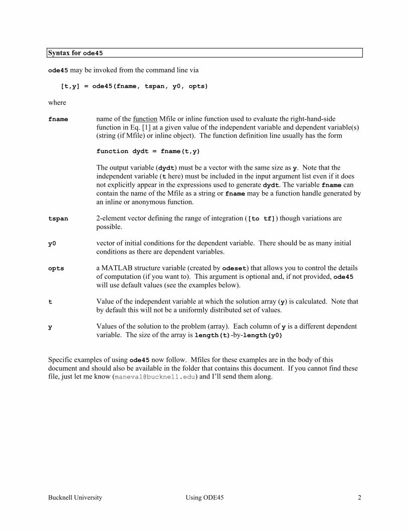
Syntax for ode45 ode45 may be invoked from the command line via [t,y] = ode45(fname, tspan, y0, opts) where fname name of the function Mfile or inline function used to evaluate the right-hand-side

function in Eq. [1] at a given value of the independent variable and dependent variable(s) (string (if Mfile) or inline object). The function definition line usually has the form function dydt = fname(t,y) The output variable (dydt) must be a vector with the same size as y. Note that the independent variable (t here) must be included in the input argument list even if it does not explicitly appear in the expressions used to generate dydt. The variable fname can contain the name of the Mfile as a string or fname may be a function handle generated by an inline or anonymous function.

tspan 2-element vector defining the range of integration ([to tf]) though variations are possible.

y0 vector of initial conditions for the dependent variable. There should be as many initial

conditions as there are dependent variables. opts a MATLAB structure variable (created by odeset) that allows you to control the details

of computation (if you want to). This argument is optional and, if not provided, ode45 will use default values (see the examples below).

t Value of the independent variable at which the solution array (y) is calculated. Note that

by default this will not be a uniformly distributed set of values. y Values of the solution to the problem (array). Each column of y is a different dependent

variable. The size of the array is length(t)-by-length(y0) Specific examples of using ode45 now follow. Mfiles for these examples are in the body of this document and should also be available in the folder that contains this document. If you cannot find these file, just let me know ([email protected]) and I’ll send them along.


Integrating a single, first-order equation The height of fluid in a tank (h(t)) whose outlet flow is dependent on the pressure head (height of fluid) inside the tank and whose inlet flow is a function of time may be modeled via the equation

€

dhdt

=α(t) − β h h(0) = ho [2]

Find the solution, h(t), for

€

0 < t < 30 if the following values for the parameters are given. Input flow:

€

α( t) =10+ 4 sin(t)

€

β = 2

€

ho =1 Step 1: Identify

€

f (t ,y) and write a MATLAB function Mfile to evaluate it. In this case, we have time as the independent variable and the tank height as the (single) dependent variable. Thus, we have

€

f (t,y)→ f (t,h) =α(t) − β h [3] From the given information for this problem, the required Mfile, named tankfill.m, is function dhdt = tankfill(t,h) % RHS function for tank-fill problem A = 10 + 4*sin(t); % alpha(t) H = 2*sqrt(h); % beta*sqrt(h) dhdt = A - H; % eof - tankfill.m Step 2: Use ode45 to solve the problem The initial condition has the height at 1 for t = 0 and we want to integrate until t = 30. The following set of commands show explicitly how the solution is put together. >> tspan = [0 30]; (integration range) >> h0 = 1; (initial condition, h(0)) >> [t,h] = ode45('tankfill',tspan,h0); (solve the problem) Step 3: Look at the solution The solution can be viewed via the plot command as in >> plot(t,h) The "curve" is a little choppy though it is accurate to the default relative tolerance (0.001). Note that the places where the solution is given are not uniformly spread out. See the next section for improving appearances.


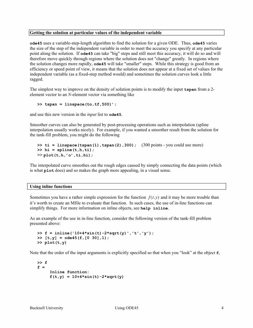
Getting the solution at particular values of the independent variable ode45 uses a variable-step-length algorithm to find the solution for a given ODE. Thus, ode45 varies the size of the step of the independent variable in order to meet the accuracy you specify at any particular point along the solution. If ode45 can take "big" steps and still meet this accuracy, it will do so and will therefore move quickly through regions where the solution does not "change" greatly. In regions where the solution changes more rapidly, ode45 will take "smaller" steps. While this strategy is good from an efficiency or speed point of view, it means that the solution does not appear at a fixed set of values for the independent variable (as a fixed-step method would) and sometimes the solution curves look a little ragged. The simplest way to improve on the density of solution points is to modify the input tspan from a 2-element vector to an N-element vector via something like >> tspan = linspace(to,tf,500)’; and use this new version in the input list to ode45. Smoother curves can also be generated by post-processing operations such as interpolation (spline interpolation usually works nicely). For example, if you wanted a smoother result from the solution for the tank-fill problem, you might do the following >> ti = linspace(tspan(1),tspan(2),300); (300 points - you could use more) >> hi = spline(t,h,ti); >> plot(t,h,’o’,ti,hi); The interpolated curve smoothes out the rough edges caused by simply connecting the data points (which is what plot does) and so makes the graph more appealing, in a visual sense. Using inline functions Sometimes you have a rather simple expression for the function

€

f (t,y) and it may be more trouble than it’s worth to create an Mfile to evaluate that function. In such cases, the use of in-line functions can simplify things. For more information on inline objects, see help inline. As an example of the use in in-line function, consider the following version of the tank-fill problem presented above:

>> f = inline('10+4*sin(t)-2*sqrt(y)','t','y'); >> [t,y] = ode45(f,[0 30],1); >> plot(t,y)

Note that the order of the input arguments is explicitly specified so that when you “look” at the object f,

>> f f = Inline function: f(t,y) = 10+4*sin(t)-2*sqrt(y)


you see that t (the independent variable) is the first input, as required by ode45 and other solvers. If you do not specify the order, inline will rely on a default method of setting the order that may not be what you want. As long as

€

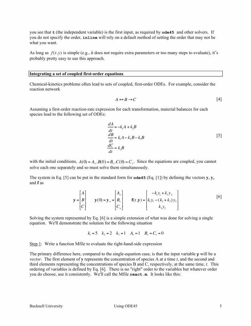
f (t,y) is simple (e.g., it does not require extra parameters or too many steps to evaluate), it’s probably pretty easy to use this approach. Integrating a set of coupled first-order equations Chemical-kinetics problems often lead to sets of coupled, first-order ODEs. For example, consider the reaction network

€

A↔B→C [4] Assuming a first-order reaction-rate expression for each transformation, material balances for each species lead to the following set of ODEs:

€

dAdt

= −k1A + k2B

dBdt

= k1A− k2B− k3B

dCdt

= k3B

[5]

with the initial conditions,

€

A(0) = Ao ,B(0) =Bo ,C(0) =Co . Since the equations are coupled, you cannot solve each one separately and so must solve them simultaneously. The system in Eq. [5] can be put in the standard form for ode45 (Eq. [1]) by defining the vectors y, yo and f as

€

y =

ABC

⎡

⎣

⎢ ⎢ ⎢

⎤

⎦

⎥ ⎥ ⎥

y(0) = y o =

Ao

BoCo

⎡

⎣

⎢ ⎢ ⎢

⎤

⎦

⎥ ⎥ ⎥

f(t ,y) =

−k1y1 + k2y 2k1y1 −(k2 + k3 )y2

k3y2

⎡

⎣

⎢ ⎢ ⎢

⎤

⎦

⎥ ⎥ ⎥

[6]

Solving the system represented by Eq. [6] is a simple extension of what was done for solving a single equation. We'll demonstrate the solution for the following situation

€

k1 = 5 k2 = 2 k3 =1 Ao =1 Bo =Co = 0 Step 1: Write a function Mfile to evaluate the right-hand-side expression The primary difference here, compared to the single-equation case, is that the input variable y will be a vector. The first element of y represents the concentration of species A at a time t, and the second and third elements representing the concentrations of species B and C, respectively, at the same time, t. This ordering of variables is defined by Eq. [6]. There is no "right" order to the variables but whatever order you do choose, use it consistently. We'll call the Mfile react.m. It looks like this:


function dydt = react(t,y) % Solve the kinetics example dydt = zeros(size(y)); % Parameters - reaction-rate constants k1 = 5; k2 = 2; k3 = 1; A = y(1); We'll be explicit about it here though you can do B = y(2); the calculations directly with the y-values. C = y(3); % Evaluate the RHS expression dydt(1) = -k1*A + k2*B; dydt(2) = k1*A - (k2+k3)*B; dydt(3) = k3*B; % eof - react.m

Note that the input arguments must be t and y (in that order) even though t is not explicitly used in the function. Step 2: Use ode45 to solve the problem No time interval is given so we'll pick one (0 to 4) and see what the solution looks like. If a longer or shorter interval is needed, we can simply re-execute the function with a new value for the ending time. Following the outline for the single-equation problem, the call to ode45 is, >> [t,y] = ode45('react',[0 4],[1 0 0]); Note that the initial condition is provided directly in the call to ode45. You could also have defined a variable y0 prior to the call to ode45 and used that variable as an input. Take a moment to look at the outputs. The number of points at which the solution is known is >> length(t) Also consider the shape of the output variable y: >> size(y) Is the result as stated above (i.e., is it length(t)-by-length(y0))? Step 3: Look at the solution If you want to see the time-course of all species, use the command >> plot(t,y) The blue line will be the first column of y (species A). The green and red lines will be the second and third columns of y (species B and C, respectively).


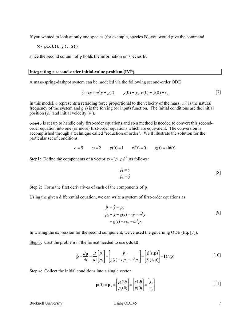
If you wanted to look at only one species (for example, species B), you would give the command >> plot(t,y(:,2)) since the second column of y holds the information on species B. Integrating a second-order initial-value problem (IVP) A mass-spring-dashpot system can be modeled via the following second-order ODE

€

˙ ̇ y + c ˙ y +ω 2y = g( t) y(0) = yo ,v (0) = ˙ y (0) = vo [7] In this model, c represents a retarding force proportional to the velocity of the mass,

€

ω2 is the natural frequency of the system and g(t) is the forcing (or input) function. The initial conditions are the initial position (yo) and initial velocity (vo). ode45 is set up to handle only first-order equations and so a method is needed to convert this second-order equation into one (or more) first-order equations which are equivalent. The conversion is accomplished through a technique called "reduction of order". We'll illustrate the solution for the particular set of conditions

€

c = 5 ω = 2 y(0) =1 v (0) = 0 g( t) = sin(t) Step1: Define the components of a vector

€

p =[p1 p2]T as follows:

€

p1 = yp2 = ˙ y

[8]

Step 2: Form the first derivatives of each of the components of p Using the given differential equation, we can write a system of first-order equations as

€

˙ p 1 = ˙ y = p2

˙ p 2 = ˙ ̇ y = g( t)− c ˙ y −ω2y= g(t) −cp2 −ω

2p1

[9]

In writing the expression for the second component, we've used the governing ODE (Eq. [7]). Step 3: Cast the problem in the format needed to use ode45.

€

˙ p = dpdt

=ddt

p1

p2

⎡

⎣ ⎢

⎤

⎦ ⎥ =

p2

g(t )− cp2 −ω2p1

⎡

⎣ ⎢

⎤

⎦ ⎥ =

f1 (t ,p)f 2( t, p)⎡

⎣ ⎢

⎤

⎦ ⎥ = f (t ,p) [10]

Step 4: Collect the initial conditions into a single vector

€

p(0) = po =p1 (0)p2 (0)⎡

⎣ ⎢

⎤

⎦ ⎥ =

y(0)˙ y (0)⎡

⎣ ⎢

⎤

⎦ ⎥ =

yo

vo

⎡

⎣ ⎢

⎤

⎦ ⎥ [11]


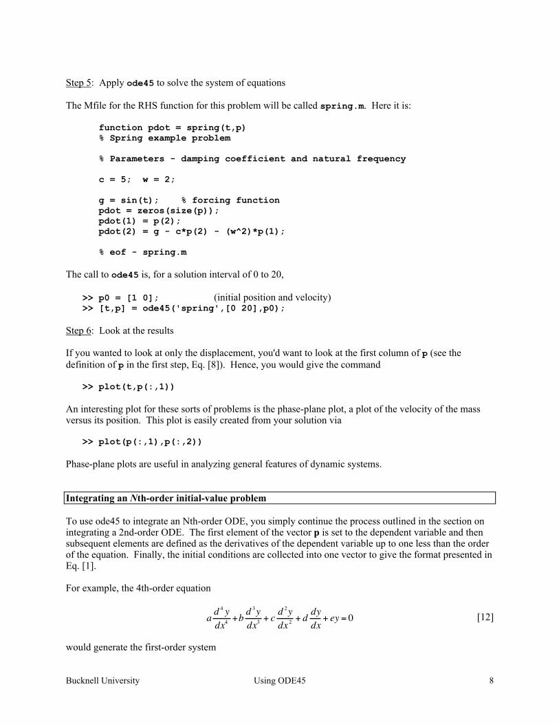
Step 5: Apply ode45 to solve the system of equations The Mfile for the RHS function for this problem will be called spring.m. Here it is:

function pdot = spring(t,p) % Spring example problem % Parameters - damping coefficient and natural frequency c = 5; w = 2; g = sin(t); % forcing function pdot = zeros(size(p)); pdot(1) = p(2); pdot(2) = g - c*p(2) - (w^2)*p(1); % eof - spring.m

The call to ode45 is, for a solution interval of 0 to 20, >> p0 = [1 0]; (initial position and velocity) >> [t,p] = ode45('spring',[0 20],p0); Step 6: Look at the results If you wanted to look at only the displacement, you'd want to look at the first column of p (see the definition of p in the first step, Eq. [8]). Hence, you would give the command >> plot(t,p(:,1)) An interesting plot for these sorts of problems is the phase-plane plot, a plot of the velocity of the mass versus its position. This plot is easily created from your solution via >> plot(p(:,1),p(:,2)) Phase-plane plots are useful in analyzing general features of dynamic systems. Integrating an Nth-order initial-value problem To use ode45 to integrate an Nth-order ODE, you simply continue the process outlined in the section on integrating a 2nd-order ODE. The first element of the vector p is set to the dependent variable and then subsequent elements are defined as the derivatives of the dependent variable up to one less than the order of the equation. Finally, the initial conditions are collected into one vector to give the format presented in Eq. [1]. For example, the 4th-order equation

€

a d4 ydx4

+b d3ydx3

+ c d2y

dx 2+ d dy

dx+ ey = 0 [12]

would generate the first-order system


€

ddt

p1p2p3p4

⎡

⎣

⎢ ⎢ ⎢ ⎢ ⎢

⎤

⎦

⎥ ⎥ ⎥ ⎥ ⎥

=

p2p3p4

−(bp4 +cp3 + dp2 + ep1 ) / a

⎡

⎣

⎢ ⎢ ⎢ ⎢ ⎢

⎤

⎦

⎥ ⎥ ⎥ ⎥ ⎥

[13]

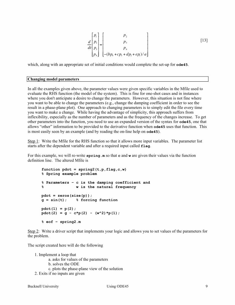
which, along with an appropriate set of initial conditions would complete the set-up for ode45. Changing model parameters In all the examples given above, the parameter values were given specific variables in the Mfile used to evaluate the RHS function (the model of the system). This is fine for one-shot cases and in instances where you don't anticipate a desire to change the parameters. However, this situation is not fine where you want to be able to change the parameters (e.g., change the damping coefficient in order to see the result in a phase-plane plot). One approach to changing parameters is to simply edit the file every time you want to make a change. While having the advantage of simplicity, this approach suffers from inflexibility, especially as the number of parameters and as the frequency of the changes increase. To get other parameters into the function, you need to use an expanded version of the syntax for ode45, one that allows “other” information to be provided to the derivative function when ode45 uses that function. This is most easily seen by an example (and by reading the on-line help on ode45). Step 1: Write the Mfile for the RHS function so that it allows more input variables. The parameter list starts after the dependent variable and after a required input called flag. For this example, we will re-write spring.m so that c and w are given their values via the function definition line. The altered Mfile is

function pdot = spring2(t,p,flag,c,w) % Spring example problem

% Parameters – c is the damping coefficient and % w is the natural frequency pdot = zeros(size(p)); g = sin(t); % forcing function pdot(1) = p(2); pdot(2) = g - c*p(2) - (w^2)*p(1); % eof – spring2.m

Step 2: Write a driver script that implements your logic and allows you to set values of the parameters for the problem. The script created here will do the following 1. Implement a loop that a. asks for values of the parameters b. solves the ODE c. plots the phase-plane view of the solution 2. Exits if no inputs are given


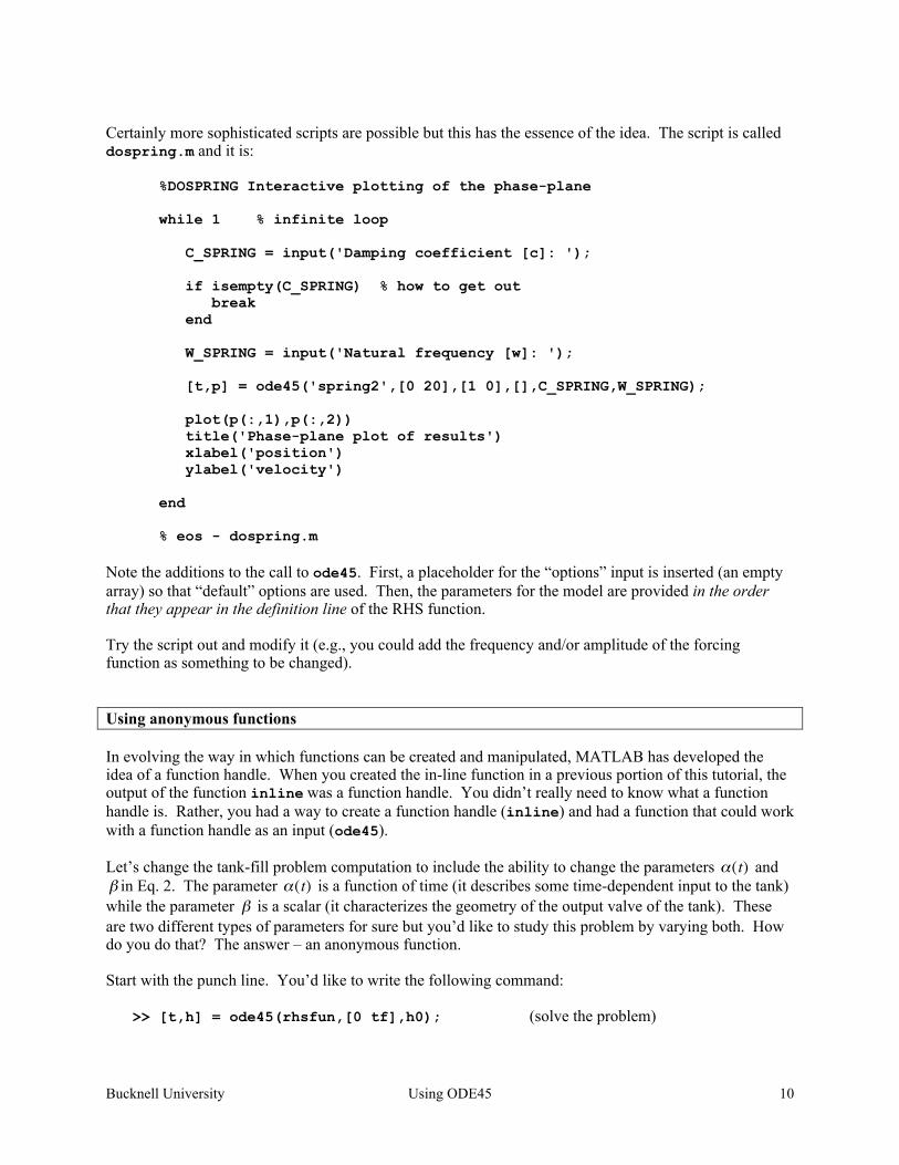
Certainly more sophisticated scripts are possible but this has the essence of the idea. The script is called dospring.m and it is:

%DOSPRING Interactive plotting of the phase-plane while 1 % infinite loop C_SPRING = input('Damping coefficient [c]: '); if isempty(C_SPRING) % how to get out break end W_SPRING = input('Natural frequency [w]: '); [t,p] = ode45('spring2',[0 20],[1 0],[],C_SPRING,W_SPRING); plot(p(:,1),p(:,2)) title('Phase-plane plot of results') xlabel('position') ylabel('velocity') end % eos - dospring.m

Note the additions to the call to ode45. First, a placeholder for the “options” input is inserted (an empty array) so that “default” options are used. Then, the parameters for the model are provided in the order that they appear in the definition line of the RHS function. Try the script out and modify it (e.g., you could add the frequency and/or amplitude of the forcing function as something to be changed). Using anonymous functions In evolving the way in which functions can be created and manipulated, MATLAB has developed the idea of a function handle. When you created the in-line function in a previous portion of this tutorial, the output of the function inline was a function handle. You didn’t really need to know what a function handle is. Rather, you had a way to create a function handle (inline) and had a function that could work with a function handle as an input (ode45). Let’s change the tank-fill problem computation to include the ability to change the parameters

€

α(t) and

€

β in Eq. 2. The parameter

€

α(t) is a function of time (it describes some time-dependent input to the tank) while the parameter

€

β is a scalar (it characterizes the geometry of the output valve of the tank). These are two different types of parameters for sure but you’d like to study this problem by varying both. How do you do that? The answer – an anonymous function. Start with the punch line. You’d like to write the following command: >> [t,h] = ode45(rhsfun,[0 tf],h0); (solve the problem)


The goal is to make sure that the object rhsfun (which will be a function handle) has everything needed to evaluate the right-hand side function for the ODE. There are several ways one might make this work. I’m going to approach it simply yet try and make it clear where you might make improvements of extensions – or apply the method to a problem of your own. As a first example, assume that the input function is a relatively simple expression, on for which an inline function might be a good match. Thus, create

€

α(t) as before and assign a value to

€

β :

a = inline('10 + 4*sin(t)','t'); b = 2;

Then create a function handle for the right-hand side function using the anonymous-function syntax

rhsfun = @(t,h) a(t)-b*sqrt(h); The syntax here is not the best (in my humble opinion) but you can get used to it – especially when it works for you. To understand what’s going on here, let’s break this line down. The @ operator (in this context) is the anonymous-function operator that creates a function handle (rhsfun) from the information that it finds to its right. Hence, you should read the line generically as

fhandle = @(<essential variable list>) <valid expression> The essential variables (t and h here) are enclosed in parentheses and are the variables in the expression that the function that uses this object (ode45 in this case) must provide in order to evaluate the expression (take a moment to let that sink in). The expression that follows is any MATLAB expression that was valid at the time the handle was created (hence the need to define the inline function a before the anonymous function was defined). The function handle that is created can then be used according to the syntax of the essential variable list. For example,

>> rhsfun(1,2) ans = 10.5375

Note that all the details of how the inputs 1 and 2 are used within the handle are disguised. You just need to provide them and the original definition of the expression (contained in the object rhsfun) does the work of sorting out how to do the evaluation. The solution to the problem can thus be compactly written as >> tf = 30; (maximum time for solution to run) >> h0 = 1; (initial condition, h(0)) >> a = inline('10 + 4*sin(t)','t'); (define the input function) >> b = 2; (the valve characteristic) >> rhsfun = @(t,h) (a(t) - b*sqrt(h)); (define the RHS function) >> [t,h] = ode45(rhsfun,[0 tf],h0); (solve the problem) >> plot(t,h) (show results)


As a final example of using anonymous function, let’s consider a case where the input is perhaps not so simple so that an inline function is just not going to cut it for computation. In addition, you have a valve with more complex characteristics than just

€

h . No problem – you are still in business. Assume that the RHS function could be computed by an Mfile you wrote that has the definition line

function a = tankfun(t,h,p1,p2) In your function, p1 and p2 are parameters you set to make the function do what it needs to do (and that’s up to you and your function). Then, an anonymous function will let you use your Mfile in the same way that the inline function was used previously. To repeat the example from above, >> tf = 30; (maximum time for solution to run) >> h0 = 1; (initial condition, h(0)) >> p1 = 2; p2 = 1; (a parameter set for this problem) >> rhsfun = @(t,h) tankfun(t,h,p1,p2); (define the RHS function) >> [t,h] = ode45(rhsfun,[0 tf],h0); (solve the problem) Note that as long as all variables used in the expression (beyond those in the essential variable list) are valid when the line defining rhsfun executes, you have successfully “captured” the expression for the right-hand side in an easy-to-evaluate version, rhsfun(t,h). Variations on this theme abound. What you do depends on the nature of the problem and the number of times you will use the model. Just be sure to follow the rule that the expression contained in the anonymous function should be valid at the time of the creation of the function handle. Integrating a second-order boundary-value problem (BVP) ode45 was written to solve initial-value problems (IVPs). Hence it cannot be (directly) used to solve, for example, the following problem derived from a model of heat-transfer in a rod:

d2ydx 2

− y = 0 y(0) = 1 dydx x =1

= 0 [14]

since the value of the derivative at x = 0 is not specified (it is known at x = 1, though). Equation [14] is a boundary-value problem (BVP) and is common in models based on transport phenomena (heat transfer, mass transfer and fluid mechanics). All is not lost because one way to solve a BVP is to pretend it is an IVP. To make up for the lack of knowledge of the derivative at the initial point, you can guess a value, do the integration and then check yourself by seeing how close you are to meeting the conditions at the other end of the interval. When you have guessed the right starting values, you have the solution to the problem. This approach is sometimes called the "shooting method" by analogy to the ballistics problem of landing an artillery shell on a target by specifying only it's set-up (powder charge and angle of the barrel). Step 1: Set up the problem so that ode45 can solve it Using the approach of turning a second order equation into a pair of coupled first-order equations, we have


€

ddx

p1p2

⎡

⎣ ⎢

⎤

⎦ ⎥ =

p2p1

⎡

⎣ ⎢

⎤

⎦ ⎥ p(0) =

1v⎡

⎣ ⎢ ⎤

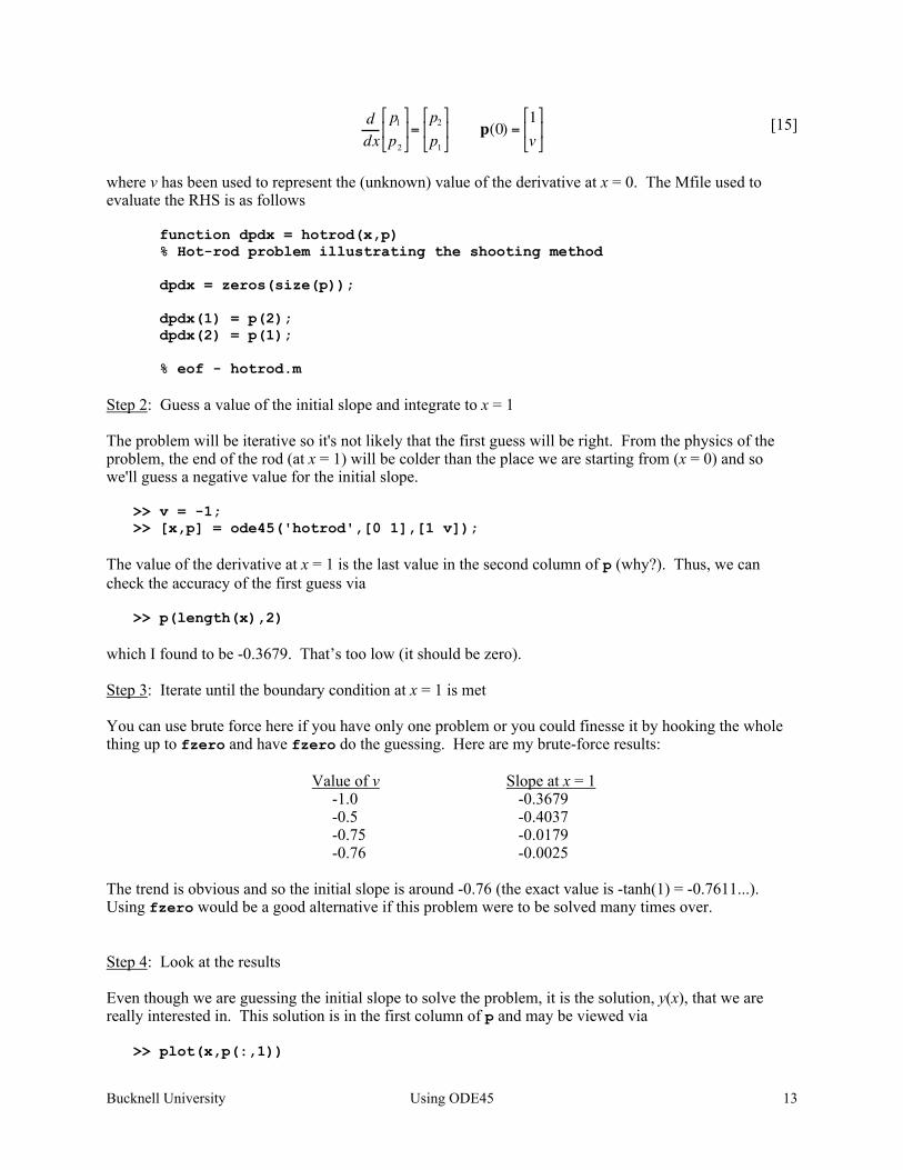
⎦ ⎥ [15]

where v has been used to represent the (unknown) value of the derivative at x = 0. The Mfile used to evaluate the RHS is as follows

function dpdx = hotrod(x,p) % Hot-rod problem illustrating the shooting method dpdx = zeros(size(p)); dpdx(1) = p(2); dpdx(2) = p(1); % eof - hotrod.m

Step 2: Guess a value of the initial slope and integrate to x = 1 The problem will be iterative so it's not likely that the first guess will be right. From the physics of the problem, the end of the rod (at x = 1) will be colder than the place we are starting from (x = 0) and so we'll guess a negative value for the initial slope. >> v = -1; >> [x,p] = ode45('hotrod',[0 1],[1 v]); The value of the derivative at x = 1 is the last value in the second column of p (why?). Thus, we can check the accuracy of the first guess via >> p(length(x),2) which I found to be -0.3679. That’s too low (it should be zero). Step 3: Iterate until the boundary condition at x = 1 is met You can use brute force here if you have only one problem or you could finesse it by hooking the whole thing up to fzero and have fzero do the guessing. Here are my brute-force results: Value of v Slope at x = 1 -1.0 -0.3679 -0.5 -0.4037 -0.75 -0.0179 -0.76 -0.0025 The trend is obvious and so the initial slope is around -0.76 (the exact value is -tanh(1) = -0.7611...). Using fzero would be a good alternative if this problem were to be solved many times over. Step 4: Look at the results Even though we are guessing the initial slope to solve the problem, it is the solution, y(x), that we are really interested in. This solution is in the first column of p and may be viewed via >> plot(x,p(:,1))


If BVP’s are a serious part of your computational problem, you should have a look at bvp4c. Setting options in ode45 The input opts is a MATLAB structure variable that con be used to control the performance of the various ODE-solvers in MATLAB. The most common option that you’ll likely want to alter is the accuracy to which solutions are computed. To make this process easy, a pair of functions are available – odeset for creating and changing options and odeget for displaying information on options. To see what the current settings are, try the command >> odeset Default values for any setting are denoted by the braces, {}. MATLAB uses two accuracy measures for solving ODEs – the relative tolerance (RelTol in opts) and the absolute tolerance (AbsTol in opts). Each step in the integration is taken so that it satisfies the condition

€

Error at step j ≤maxk(RelTol ⋅ y jk ,AbsTolk )

where the subscript k ranges over all the components of the solution vector at time step j. To alter the default settings, use commands such as >> oldOpts = odeset; >> newOpts = odeset(oldOpts,’RelTol’,1e-6) Information on the settings for the other options is available in the on-line help. Going beyond ode45 The solver ode45 is not the be-all and end-all of ODE-solvers. While ode45 should be your first choice for integration, there are problems that the function performs poorly on or even fails on. In such cases, there are fallback solvers that are available. All these solvers use the same syntax as ode45 (see page 2) but have options for handling more difficult or sophisticated problems. Here are some suggestions for handling non-standard ODE problems:

• If accuracy you desire is not obtainable via ode45, try the function ode113. This solver uses a variable order method that may be able to improve over what ode45 does.

• If ode45 is taking too long to compute a solution, your problem may be “stiff” (i.e., it involves a

system with a wide range of time constants). Try the function ode15s. • If your system of equations has the form

€

M dydt

= f( t,y)


where M is a (typically non-singular) matrix, try the function ode15s.

• In newer versions of MATLAB, the function bvp4c is available for solving boundary-value problems.

You’ll find more information on these functiona in the on-line help and documentation. For example, try the on-line function reference (available through the command helpdesk) on any of the solvers noted above.

bucknell university using ode45 matlab helptang.eece.wustl.edu/kirk/maneval ode45.pdf · bucknell...

Documents