biomechanics of sprint running: a methodological...

Co-tutoring PhD program in Bioengineering

XXIII Cycle – ING-INF/06

Administrative Universities: Università degli Studi di Bologna (Bologna) – Arts et Métiers ParisTech (Paris)

Associate University: Università degli Studi di Roma “Foro Italico”, ex Istituto Universitario di Scienze Motorie (Roma)

Biomechanics of sprint running:

a methodological contribution

Elena Bergamini

Supevisors: Prof. Aurelio Cappozzo Università degli Studi di Roma “Foro Italico”

Prof. Wafa Skalli Arts et Métiers ParisTech

Dr. Valentina Camomilla Università degli Studi di Roma “Foro Italico”

Dr. Hélène Pillet Arts et Métiers ParisTech

Coordinator: Prof. Angelo Cappello Università degli Studi di Bologna

Co-examiner: Prof. Luca Cristofolini Università degli Studi di Bologna

v

CONTENTS

PREFACE................................................................................................................................................ ix

ABSTRACT ............................................................................................................................................ xi

ENGLISH VERSION...................................................................................................................xi

ITALIAN VERSION.................................................................................................................. xii

FRENCH VERSION.................................................................................................................xiii

EXTENDED SUMMARY................................................................................................................... xv

CHAPTER 1 – THEORETICAL BACKGROUND .................................................................. - 1 -

ABSTRACT.............................................................................................................................. - 2 -

1.1 INTRODUCTION ........................................................................................................... - 4 -

1.2 SPRINT RUNNING BIOMECHANICS: PERFORMANCE AND INJURY-

RELATED VARIABLES ....................................................................................................... - 6 -

1.2.1 Block start phase............................................................................................. - 7 -

1.2.2 Acceleration or pick-up phase ..................................................................- 14 -

1.2.3 Maintenance phase ......................................................................................- 18 -

1.2.4 Deceleration phase .......................................................................................- 26 -

1.3 METHODS FOR SPRINT RUNNING ANALYSIS ................................................- 27 -

1.3.1 Electromyography ........................................................................................- 28 -

1.3.2 Motion analysis (Stereophotogrammetry)...........................................- 30 -

1.3.3 Force plates.....................................................................................................- 31 -

1.3.4 Pressure sensors ............................................................................................- 31 -

1.3.5 Accelerometers ..............................................................................................- 32 -

1.3.6 Gyroscopes.......................................................................................................- 34 -

1.3.7 Electrogoniometers ......................................................................................- 35 -

1.4 THEORETICAL BACKGROUND: DISCUSSION..................................................- 36 -

vi

CHAPTER 2 - AIM OF THE THESIS ..................................................................................... - 37 -

CHAPTER 3 - LOW RESOLUTION APPROACH .............................................................. - 39 -

ABSTRACT............................................................................................................................- 41 -

3.1 INTRODUCTION .........................................................................................................- 42 -

3.1.1 Sports biomechanics and in-field performance evaluation ............- 42 -

3.1.2 Wearable inertial sensors ..........................................................................- 45 -

3.2 STUDY 1: TRUNK INCLINATION DURING THE SPRINT START USING AN

INERTIAL MEASUREMENT UNIT ...............................................................................- 49 -

Abstract ......................................................................................................................- 49 -

3.2.1 Introduction....................................................................................................- 50 -

3.2.2 Materials and methods ...............................................................................- 52 -

3.2.3 Results...............................................................................................................- 58 -

3.2.4 Discussion ........................................................................................................- 60 -

3.3 STUDY 2: INSTANTANEOUS VELOCITY AND CENTER OF MASS

DISPLACEMENT OF IN-LAB SPRINT RUNNING USING AN INERTIAL

MEASUREMENT UNIT.....................................................................................................- 62 -

Abstract ......................................................................................................................- 62 -

3.3.1 Introduction....................................................................................................- 63 -


3.3.3 Results...............................................................................................................- 65 -

3.3.4 Discussion ........................................................................................................- 66 -

3.4 STUDY 3: TEMPORAL PARAMETERS OF IN-FIELD SPRINT RUNNING

USING AN INERTIAL MEASUREMENT UNIT..........................................................- 68 -

Abstract ......................................................................................................................- 68 -

3.4.1 Introduction....................................................................................................- 69 -


3.4.3 Results...............................................................................................................- 74 -

3.4.4 Discussion ........................................................................................................- 80 -

3.5 LOW RESOLUTION APPROACH: DISCUSSION................................................- 83 -

CHAPTER 4 - HIGH RESOLUTION APPROACH .............................................................- 85 -

ABSTRACT............................................................................................................................- 87 -

vii

4.1 INTRODUCTION .........................................................................................................- 88 -

4.1.1 Sport biomechanics and injury prevention ..........................................- 88 -

4.1.2 Joint dynamics estimation..........................................................................- 92 -

4.2 STUDY 4: TIBIO-FEMORAL JOINT CONSTRAINTS FOR BONE POSE

ESTIMATION DURING MOVEMENT USING MULTI-BODY OPTIMIZATION- 94 -

Abstract ......................................................................................................................- 94 -

4.2.1 Introduction....................................................................................................- 95 -


4.2.3 Results............................................................................................................ - 101 -

4.2.4 Discussion ..................................................................................................... - 104 -

4.3 HIGH RESOLUTION APPROACH: DISCUSSION............................................ - 107 -

CHAPTER 5 - CONCLUSIONS .............................................................................................. - 109 -

AKNOWLEDGEMENTS .......................................................................................................... - 113 -

REFERENCES ............................................................................................................................. - 117 -

ix

PREFACE

Sports biomechanics uses the scientific methods of mechanics to study the

internal and external forces acting on a human body and the effects produced by

these forces in sports activities. It is, therefore, concerned, with the ways in which

sports movements are performed, often referred to as sports techniques.

With this respect, sports biomechanics has an applicative nature and it has

an ultimate objective: the achievement of an effective technique. Indeed, while it is

often believed that the main goal of sports biomechanists and coaches is to obtain

the best athlete’s performance, it must be kept in mind that performance

enhancement and injury risk are strictly related. If improving the athlete’s

performance would entail increasing the risk of injury, no actual effective

improvement would be obtained. This is the reason why sports biomechanics is

often described as having two aims that may be perceived as incompatible: the

reduction of the risk of injury (such as identification of the causes of back injuries

in cricket, or the causes of knee joint injuries in sprint running) and the

improvement of performance (such as optimising gymnastics performance

through simulation of in-flight movements, or studying the effects of tennis racquet

stiffness on the performance of young athletes).

Although sports biomechanists and coaches, as well as athletes and

physicians, share exactly the same objectives, there is still a gap between

researchers and practitioners. Coaches commonly base their evaluation of athletes’

performance and of the efficacy of their training program on competition results,

field tests and qualitative visual inspection. Such evaluations are often readable,

easy to use and they provide information about the global performance.

Nevertheless, they are often not able to establish an understanding of causal

mechanisms for the selected movements (such as the role of internal rotation of

the upper arm in hitting or striking, or the influence of elastic energy and muscle

pre-stretch in stretch-shorten-cycle actions). On the other hand, biomechanists,

accused to be over-concerned with methodology, often lack of pragmatism.

x

In order to bridge the gap between the two worlds, the establishment of a

common and understandable language is crucial. The importance of quantitative

assessment of athletes’ motor skills needs to be well perceived by coaches, as well

as by athletes and sports physicians. At the same time, biomechanists must be able

to fully understand the actual needs of practitioners and find the appropriate way

to communicate and propose their results.

There are two main limitations that have to be overcome in order to achieve

these goals: first, the difficulties in performing in-field athlete evaluation and in

obtaining data in a natural setting such as competition, without influencing or

constraining athletes’ activities. To date, in fact, sports biomechanical analysis is

typically performed by means of stereophotogrammetry, force platforms, high-

speed cameras, or optical contact time meters. Such solutions, however, are

expensive, characterized by a cumbersome and time-consuming experimental set

up and tend to constrain the subject and the analysed motor task. Second, there is

a lack of methods specifically designed for sports applications, even when dealing

with marker-based motion analysis. Protocols commonly developed for clinical

biomechanical assessment, in fact, could hardly be transposed to the analysis of

sports motor acts, which are characterized by higher accelerations and

explosiveness with respect to the former.

In this framework, the present thesis aims at providing a contribution in

these directions, focusing on the development of methodologies which could help

in overcoming the above mentioned limitations, filling the gap between

researchers and practitioners.

xi

ABSTRACT

ENGLISH VERSION

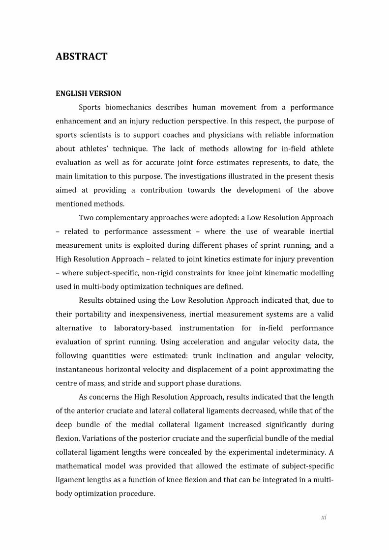
Sports biomechanics describes human movement from a performance

enhancement and an injury reduction perspective. In this respect, the purpose of

sports scientists is to support coaches and physicians with reliable information

about athletes’ technique. The lack of methods allowing for in-field athlete

evaluation as well as for accurate joint force estimates represents, to date, the

main limitation to this purpose. The investigations illustrated in the present thesis

aimed at providing a contribution towards the development of the above

mentioned methods.

Two complementary approaches were adopted: a Low Resolution Approach

– related to performance assessment – where the use of wearable inertial

measurement units is exploited during different phases of sprint running, and a

High Resolution Approach – related to joint kinetics estimate for injury prevention

– where subject-specific, non-rigid constraints for knee joint kinematic modelling

used in multi-body optimization techniques are defined.

Results obtained using the Low Resolution Approach indicated that, due to

their portability and inexpensiveness, inertial measurement systems are a valid

alternative to laboratory-based instrumentation for in-field performance

evaluation of sprint running. Using acceleration and angular velocity data, the

following quantities were estimated: trunk inclination and angular velocity,

instantaneous horizontal velocity and displacement of a point approximating the

centre of mass, and stride and support phase durations.

As concerns the High Resolution Approach, results indicated that the length

of the anterior cruciate and lateral collateral ligaments decreased, while that of the

deep bundle of the medial collateral ligament increased significantly during

flexion. Variations of the posterior cruciate and the superficial bundle of the medial

collateral ligament lengths were concealed by the experimental indeterminacy. A

mathematical model was provided that allowed the estimate of subject-specific

ligament lengths as a function of knee flexion and that can be integrated in a multi-

body optimization procedure.

xii

ITALIAN VERSION

La biomeccanica dello sport descrive il movimento umano con l’obiettivo di

migliorare la prestazione atletica e di ridurre l’incidenza di infortuni. In questo

contesto, lo scopo degli esperti di scienze dello sport è quello di fornire ad

allenatori e medici informazioni affidabili sulla tecnica di esecuzione del gesto

sportivo in esame. La mancanza di metodi che consentano la valutazione dell’atleta

direttamente sul campo e la stima accurata della dinamica articolare costituisce, ad

oggi, il principale limite nel raggiungimento di questo scopo. La presente tesi si

propone di fornire un contributo allo sviluppo di tali metodi.

Il lavoro si articola secondo due approcci complementari: un Approccio a

Bassa Risoluzione - legato alla valutazione della prestazione – attraverso il quale è

stato esplorato l'uso di sensori inerziali indossabili durante diverse fasi della corsa

di velocità, e un Approccio ad Alta Risoluzione - relativo alla stima della dinamica

articolare per la prevenzione degli infortuni - dove sono stati definiti vincoli non

rigidi per un modello cinematico del ginocchio da integrare in tecniche di

ottimizzazione multi-segmento per la stima della posizione e dell’orientamento

delle ossa durante il movimento.

I risultati ottenuti con l’Approccio a Bassa Risoluzione indicano che, in virtù

della loro portabilità ed economicità, i sensori inerziali rappresentano una valida

alternativa alla tradizionale strumentazione di laboratorio per la valutazione della

prestazione durante la corsa. Utilizzando i dati di accelerazione e velocità angolare

provenienti dai sensori, sono stati stimati l’inclinazione e la velocità angolare del

tronco, la velocità lineare istantanea e lo spostamento di un punto che approssima

il centro di massa, e le durate della fase di appoggio e del ciclo del passo.

Per quanto riguarda l'Approccio ad Alta Risoluzione, i risultati indicano che

le lunghezze del legamento crociato anteriore e del collaterale laterale

diminuiscono, mentre quella del fascio profondo del legamento collaterale mediale

aumenta durante la flessione. Le variazioni di lunghezza del legamento crociato

posteriore e del fascio superficiale del legamento collaterale mediale sono risultate

dello stesso ordine dell’errore sperimentale. Al fine di integrare tali informazioni in

una procedura di ottimizzazione multi-segmento, è stato definito un modello

matematico del ginocchio che fornisce le lunghezze plausibili dei legamenti in

funzione dell’angolo di flessione.

xiii

FRENCH VERSION

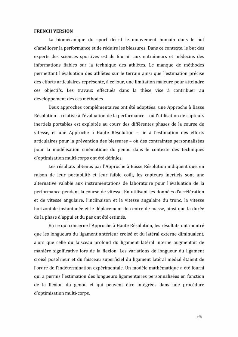
La biomécanique du sport décrit le mouvement humain dans le but

d’améliorer la performance et de réduire les blessures. Dans ce contexte, le but des

experts des sciences sportives est de fournir aux entraîneurs et médecins des

informations fiables sur la technique des athlètes. Le manque de méthodes

permettant l'évaluation des athlètes sur le terrain ainsi que l'estimation précise

des efforts articulaires représente, à ce jour, une limitation majeure pour atteindre

ces objectifs. Les travaux effectués dans la thèse vise à contribuer au

développement des ces méthodes.

Deux approches complémentaires ont été adoptées: une Approche à Basse

Résolution – relative à l'évaluation de la performance – où l'utilisation de capteurs

inertiels portables est exploitée au cours des différentes phases de la course de

vitesse, et une Approche à Haute Résolution – lié à l’estimation des efforts

articulaires pour la prévention des blessures – où des contraintes personnalisées

pour la modélisation cinématique du genou dans le contexte des techniques

d'optimisation multi-corps ont été définies.

Les résultats obtenus par l'Approche à Basse Résolution indiquent que, en

raison de leur portabilité et leur faible coût, les capteurs inertiels sont une

alternative valable aux instrumentations de laboratoire pour l'évaluation de la

performance pendant la course de vitesse. En utilisant les données d'accélération

et de vitesse angulaire, l’inclinaison et la vitesse angulaire du tronc, la vitesse

horizontale instantanée et le déplacement du centre de masse, ainsi que la durée

de la phase d’appui et du pas ont été estimés.

En ce qui concerne l'Approche à Haute Résolution, les résultats ont montré

que les longueurs du ligament antérieur croisé et du latéral externe diminuaient,

alors que celle du faisceau profond du ligament latéral interne augmentait de

manière significative lors de la flexion. Les variations de longueur du ligament

croisé postérieur et du faisceau superficiel du ligament latéral médial étaient de

l’ordre de l'indétermination expérimentale. Un modèle mathématique a été fourni

qui a permis l'estimation des longueurs ligamentaires personnalisées en fonction

de la flexion du genou et qui peuvent être intégrées dans une procédure

d'optimisation multi-corps.

xv

EXTENDED SUMMARY

INTRODUCTION AND AIM OF THE THESIS

Sports biomechanics describes the human movement from a performance


sports scientists is to support coaches and physicians with reliable and usable

information related to the athletes’ correct or incorrect technique.

Biomechanical research in sports has usually produced interesting

descriptions of the basic kinematic and kinetic features of specific athletic

movements, in order to find possible solutions for performance enhancement and,

to a lesser extent, for injury prevention. Unfortunately, these surveys have often

lacked either in providing a theoretical rationale or in presenting results that could

be directly understood and practically used by trainers and athletes. The lack of

methods and protocols allowing for in-field athlete evaluation as well as for

accurate joint forces estimate represents, to date, the main reasons of this failure.

The main purpose of the present thesis is to provide a contribution towards

the development of such methods, focusing, in particular, on sprint running

evaluation. Two complementary approaches are adopted: a Low Resolution

Approach, where the use of wearable inertial measurement units are exploited

during different phases of sprint running, and a High Resolution Approach, where

subject-specific, non-rigid constraints for knee joint kinematic modelling used in

multi-body optimization techniques are defined.

LOW RESOLUTION APPROACH

The evaluation of athlete’s performance is one of the main issues of

coaching, as well as of sports biomechanical analysis. To this aim, in-field

assessment of the athlete performance, without influencing or constraining

athletes’ activities, is now becoming mandatory.

Among the new wearable and lightweight technologies allowing for such

assessment, inertial measurement units (IMUs) appear to be a good compromise

between practicality and accuracy. These sensors combine three-axial

accelerometers and gyroscopes, and, when a measure of a global reference frame is

required, a magnetometer is also implemented. They allow data collection during

xvi

unconstrained continuous movement over prolonged periods of time, potentially

even during training and competition. Nevertheless, the extraction of movement-

related information from the signal derived from IMUs can be strongly jeopardized

by offset errors that rapidly accumulate over time (Woodman, 2007) and sensor

wide oscillations caused by the inertia of soft tissues (de Leva & Cappozzo, 2006;

Forner-Cordero et al., 2008).

The use of such sensors was explored in three studies aiming at estimating

performance-correlated biomechanical variables during the different phases of

sprint running (block-start, pick-up or acceleration, and maintenance phases). Ad-

hoc methods aimed at reducing the above mentioned sources of error were

defined. In particular, the trunk inclination and angular velocity, as well as the

instantaneous horizontal velocity and displacement of the center of mass will be

estimated during in-lab sprint running. The stride and stance durations will be

assessed on-the-field during the maintenance phase.

Study one – Trunk inclination during the sprint start

The execution of the start is crucial in determining the performance during

sprint running. Although trunk inclination is acknowledged to be a key element in

moving from the crouch to the upright position, only few study focused on this

parameter during the block start and the pick-up phases (Mero, Luhtanen, & Komi,

1983; Čoh, Jošt, Škof, Tomažin, & Dolenec, 1998; Slawinski, Bonnefoy, & Levêque,

2010).

The purpose of this study was to provide coaches with an instrument able

to reliably estimate such parameter in-field. To this aim, the accuracy of an inertial

measurement unit (IMU) in estimating its rotation about a local axis (referred to as

“quality”) and the relationship between this rotation and trunk inclination in the

progression plane (referred to as “consistency”) were assessed during block start

and pick-up phases.

Five male sprinters performed four in-lab sprint starts. The block start

phase and the first three steps of the pick-up phase were analysed. Data provided

by an IMU (FreeSense, Sensorize Ltd, Italy) positioned on the trunk at L2 level

were compared to reference stereophotogrammetric measurements. To reduce

soft tissue oscillations, a memory foam material and an elastic belt were used. The

xvii

trunk was modeled as a rigid segment joining C7 and the midpoint between the

posterior superior iliac spines. The inclination of the unit (pitch angle: β) was

estimated by combining the information provided by both the accelerometer,

during the static phases of the movement, and the gyroscope, during the non-static

phases. To improve the accuracy of such estimate, a Kalman algorithm (Kalman,

1960; Jurman, Jankovec, Kamnik, & Topic, 2007) was designed to automatically

identify these static and non-static phases and to use a proper combination of the

information provided by the two sensors. Root Mean Squared Errors, Pearson’s

correlation coefficient and Bland and Altman method (Nevill & Atkinson, 1997)

were used to assess the quality and consistency of the estimates.

Figure 1: Typical pitch angles (β) for one trial as obtained from the IMU (solid line) and from the stereophotogrammetric system: IMU reference frame (dotted line) and trunk reference frame (dashed line). The different phases of the start are also indicated: OYM: “on your marks” position; TNS: transition phase; SET: “set” position, and PICK-UP: pick-up phase. The pitch angular displacement was considered to be zero when the unit was in a horizontal position; positive angles correspond to clockwise rotations.

The quality of the IMU estimates and their consistency with trunk

inclination were high both in terms of curve similarity (correlation r>0.99) and

bias (lower than 1 and 4 deg, respectively) (Fig. 1). The agreement between the

unit and the trunk inclination, moreover, seems to support track and field coaches’

approach in considering the trunk as a rigid segment. These results open a

xviii

promising scenario for an accurate in-field use of IMUs for sprint start

performance assessment.

Study two – Center of mass instantaneous velocity and displacement during the

acceleration phase

When the focus is on sprint running performance determinants and limiting

factors, biomechanical parameters as the stance duration, the step length and the

center of mass (CoM) instantaneous velocity are crucial. Although these variables

should be obtained by numerically integrating the acceleration signal provided, for

instance, by inertial measurement units, in practice, offset errors that rapidly

accumulate over time (Woodman, 2007) yield to unreliable velocity and, therefore,

displacement.

The purpose of the study was to estimate the instantaneous horizontal

velocity and displacement of a point approximating the CoM during sprint running

by using a single inertial sensor. To this aim, a methodology for reducing the

effects of the above mentioned errors was developed. Low frequency errors were

compensated by reducing the numerical integration interval to the stance phase

and by predicting the kinematics of the sensor during the flight phase. The initial

conditions of the integration process were, then, cyclically determined.

Six sprinters performed three in-lab sprint runs, starting from a standing

position. Due to limited laboratory volume only the first three steps were analysed.

An IMU (MTx, Xsens, Netherlands) was positioned on the back trunk.

Stereophotogrammetry and force platforms were used to validate final results.

Reference and inertial sensors data were collected simultaneously at 100 samples

per second. The instantaneous progression velocity and displacement were

computed by numerical integration of the acceleration. The integration was limited

to the stance phase only, to avoid the drift typical of the integration process.

During the flight phase, the horizontal kinematics of the IMU was predicted using

the ballistic law of motion; the velocity at the instant of take-off was the last value

of the previously integrated acceleration. This procedure was reiterated for each

step. The stance time (ST), CoM progression displacement (d) and the mean

progression velocity (v) were estimated and compared with reference data. The

xix

method reliability was assessed by mean of multiple statistical tests (Multivariate

ANOVA, Pearson’s correlation coefficient, two-tailed paired t-test).

Results showed a high correlation (r>0.9) between IMU and reference

estimates for each parameter (Fig. 2). No statistical differences were found

between IMU and reference for v and ST.

Figure 2: Instantaneous progression velocity as obtained by the reference measurements (solid line), computed by numerical integration of the acceleration for the whole duration of the task (dashed line) and with the algorithm proposed in this study (dashed line). Vertical dashed lines identify the flight phases (f1, f2 and f3).

The methodology proved to successfully compensate the numerical

integration errors during in-lab non steady-state running. In-field validation is

binding in order to provide track and field coaches with reliable and accurate

information.

Study three – Temporal parameters during the maintenance phase

In the literature, walking and distance running temporal parameters have

been generally determined by identifying mechanically-related features in the

acceleration signal waveforms (Auvinet, Gloria, Renault, & Barrey, 2002; Kavanagh

& Menz, 2008; Wixted, Billing, & James, 2010). Robustness and reliability of these

temporal estimates, however, highly depends on the signal to noise ratio,

especially unfavourable during sprint running analysis as the explosiveness of the

task causes greater movements of the IMU relative to the underlying skeleton

(Pain & Challis, 2006). For this reason, sprint running analysis is more challenging

than walking or distance running.

xx

The aim of the study was to identify recognizable and consistent features in

the waveform of the signals supplied by a trunk mounted IMU, or thereof derived,

for the estimation of stance duration during in-field sprint running.

Six amateur (group A) and five elite (group B) athletes performed three 60

m sprint runs on-the-track, starting from a standing position. Four steps at each

athlete maximal speed were analysed. An IMU (FreeSense, Sensorize Ltd, Italy)

containing a 3D accelerometer and gyroscope was positioned on the lower back

trunk at L2 level with an ad-hoc elastic belt. To limit the unit oscillations relative to

the underlying bone, a memory foam material was placed between the

paravertebral muscles and the IMU (Fig. 3). Data provided by the IMU, acquired at

200 samples per second, were compared to reference forceplate and high-speed

camera measurements. The magnitude of the acceleration (a) and angular velocity

(ω) vectors as well as their 1st ( a& and ω& ) and 2nd ( a&& and ω&& ) wavelet-mediated

derivatives were computed (Jianwen, Jing, & Jinhua, 2006). Features adequate for

automatic detection of Foot-Strike (FS) and Foot-Off (FO) instants were identified

and, thereafter, used to estimate the stance (dstance) and stride (dstride) durations.

Repeated-measure ANOVA tests and Bland and Altman method (Nevill & Atkinson,

1997) were used to assess the accuracy of the estimates.

No repeatable and quantifiable features, adequate for automatic detection,

were identified in either a or its derivatives. Conversely, the magnitude of the

angular velocity signal was characterized by a consistent positive peak which

occurred approximately at the end of each step cycle in both groups of athletes.

This peak was clearly visible even by simple visual inspection of the signal and

could be used to estimate dstride (Fig. 4).

Figure 3: Belt and sensor unit location on the lower back trunk of an elite athlete of group B. Indication of the memory foam material location is also provided.

xxi

Figure 4: ω (grey dotted line), ω& (dashed line) and ω&& (solid line) with reference to a randomly chosen subject of amateur athletes (group A). Grey sections represent three consecutive stance phases.

The beginning and end of the stance were identified from positive and

negative peaks on ω&& waveform (Fig. 4). These peaks were found to be consistently

synchronized with FS and FO across steps, trials, subjects and groups. The mean of

the absolute bias between the reference and the IMU estimates was found to be in

the order of the temporal resolution of the IMU (0.005 s). It can be speculated that

increasing that resolution may improve the final results. As track and field coaches’

requirement is to obtain the stance time profile over time and during the whole

race, future works will concern the validation of the method on different phases of

the sprint run.

HIGH RESOLUTION APPROACH

A clear understanding of the definitive relationships between

biomechanical measures and injury onset in sprint running would lead to better

injury prevention strategies and would help track and field coaches to define

effective training programs. In this respect, forces and force-related factors appear

to be the prime agents that determine the likelihood and severity of injury.

Epidemiological studies of sprint running injuries, in particular, found the knee to

be the most frequent site of injuries (Brunet, Cook, Brinker, & Dickinson, 1990).

xxii

The estimate of knee joint forces during running would be, therefore, of great help

for athletes, coaches and physicians.

The accuracy of inverse dynamics methods, often used in sports

biomechanics to estimate internal and external forces, is affected by several

sources of error. Among them, the motion of soft tissues relative to the underlying

bones (soft tissue artefact – STA) is considered as the most important, particularly

in sports applications. Different techniques have been proposed to compensate for

STA. The multi-body optimization (MBO) method, in particular, aims at optimally

estimating the location in space of a chain of bones interconnected in joints. Each

joint is modelled by embedding specified constraints. To date, MBO has been

performed using spherical, revolute or universal joint constraints (Lu & O'Connor,

1999; Andersen, Damsgaard, & Rasmussen, 2009), as well as using a parallel

mechanisms (Duprey, Cheze, & Dumas, 2010). In light of recent results reported in

the literature (Andersen, Damsgaard, & Rasmussen, 2009; Duprey, Cheze, &

Dumas, 2010), the choice of joint constraints appears to be crucial.

Study four - Tibio-femoral joint constraints for multi-body optimization

To further improve the quality of knee joint models used in the MBO

approach, the definition of non-rigid constraints which take into account the

anatomy of the subject appear to be ideal. The aim of the study was to provide

plausible, subject-specific values for the distances between the origin and insertion

landmarks of the main knee ligaments (referred to as “ligament lengths”), during

loaded continuous knee flexion-extension.

Two orthogonal digital radiographs of six knee specimens (femur, tibia,

patella and fibula) were acquired using a low dosage X-ray system (EOS®, EOS-

imaging, France). The 3D geometry of each specimen was then obtained by means

of a reconstruction algorithm (Chaibi et al., 2011). The areas of origin and insertion

of the anterior and posterior cruciate, lateral collateral, and deep and superficial

bundles of the medial collateral ligaments (ACL, PCL, LCL, MCLdeep, MCLsup) were

identified on femur and tibia templates using the mouse pointer by three expert

orthopaedic surgeons (virtual palpation). Attachments sites were estimated for the

six reconstructed knees by matching the bone templates to the low dosage

stereoradiography images. Movement data of the specimens were obtained by

xxiii

means of a stereophotogrammetric system (Polaris, Nothern Digital Inc., Canada),

using pins carrying a cluster of markers and inserted into the femur and the tibia.

Data were, therefore, free from skin movement artefacts. For each knee, the

centroids of the attachment areas of each ligament were determined and the

Euclidean distance between the origin and insertion centroids computed (dc). The

impact of the inaccuracies associated with the virtual palpation was assessed

performing a Monte Carlo simulation. The Euclidean distance between each

possible couple of the points thus generated (100*100 couples) was also computed

during knee motion (dMC) (Fig. 5). Ligament length variations (∆dMC) were then

calculated relative to the distances at knee full extension and expressed as

percentage of the latter value for each sampled knee flexion angle.

Figure 5: 3D digital model of one knee specimen: the ligament attachment areas and the tibio-femoral distances between the centroids (dc) (yellow lines) as well as between selected Monte Carlo pairs (dMC) (red lines) are depicted.

The mean and standard deviation (SD) curves of ∆dMC are shown in Fig. 6

for each ligament. To facilitate embedding this information in the knee kinematic

model to be used in the MBO process, the mean of the ∆dMC curves vs flexion angle

thus obtained, plus and minus one standard deviation, were fitted with a

polynomial regression function of the fifth order. The ACL and LCL lengths were

found to decrease, and the MCLdeep length to increase significantly during flexion,

while PCL and MCLsup length trend of variation was concealed by the

xxiv

experimental indeterminacy. A mathematical model was provided that allowed the

estimate of subject-specific ligament lengths as a function of knee flexion and that

can be integrated in a multi-body optimization procedure. The efficacy of this

model, as opposed to those already implemented, must be evaluated in terms of

consequences on the estimate of joint kinetics, particularly when the inertial

effects of soft tissue masses are involved.

Figure 6: Distance variation patterns (mean ± 1SD) vs the knee flexion angle as obtained through the Monte Carlo simulation for each ligament, ∆dMC. Each variation is expressed as a percentage of the distance at knee maximal extension.

xxv

CONCLUSIONS

In the framework of sports biomechanics analysis, the results and the

considerations carried out in the present thesis aim at providing a contribution

towards the development of methods for in-field athlete evaluation as well as for

accurate joint forces estimate.

Results about the Low Resolution Approach indicate that, due to their

portability and inexpensiveness, inertial measurement units are a valid alternative

to traditional laboratory-based instrumentations for in-field performance

evaluation of sprint running. Using acceleration and angular velocity data, the

following quantities were estimated: trunk inclination and angular velocity,

instantaneous horizontal velocity and displacement of a point approximating the

CoM, and stride and stance durations. In order to limit the motion of the soft tissue

masses relative to the underlying bones, careful attention has to be paid to the

location and method of fixation of the sensor. The use of memory foam materials

and elastic belts appears to be effective. To limit the errors yielded by the unstable

bias of the signal, the integration interval should be reduced, and boundary

conditions used to cyclically correct the drift errors explored.

Results about the High Resolution Approach indicate that, in a kinematic

model of the knee based on joint constraints, the length of the ACL, LCL and

MCLdeep should be considered as variable during knee flexion. The length of the

PCL and of the MCLsup was found to be highly dependent from the selected

attachment sites. These ligaments could be, therefore, considered isometric during

knee flexion. These results represent a first contribution to the definition of

methods aiming at improving the accuracy of inverse dynamic estimates. On the

other hand, as the MBO approach aims at providing an optimal estimate of the 3D

position of a bone-chain, the reconstruction of the soft tissue movements may be

attempted. A biodynamic model of the human body based on the reconstructed

movement could then be developed. The combination of subject-specific

constraint-based joint models with such biodynamic model appears to justify the

investment of resources aimed at improving the MBO approach.

xxvi

REFERENCES

Andersen, M.S., Damsgaard, M., & Rasmussen, J. (2009). Kinematic analysis of over-determinate biomechanical systems. Computer Methods in Biomechanics and Biomedical Engineering, 12(4), 371-384.

Auvinet, B., Gloria, E., Renault, G., & Barrey, E. (2002). Runner’s stride analysis: comparison of kinematic and kinetic analyses under field conditions. Science & Sports, 17, 92-94.

Brunet, M. E., Cook, S. D., Brinker, M. R., & Dickinson, J. A. (1990). A survey of running injuries in 1505 competitive and recreational runners. Journal of Sports Medicine and Physical Fitness, 30(3), 307-315.

Chaibi, Y., Cresson, T., Aubert, B., Hausselle, J., Neyret, P., Hauger, O., & Skalli, W. (2011). Fast 3D reconstruction of the lower limb using a parametric model and statistical inferences and clinical measurements calculation from biplanar X-rays. Computer Methods in Biomechanics and Biomedical Engineering, in press.

Čoh, M., Jošt, B., Škof, B., Tomažin, K., & Dolenec, A. (1998). Kinematic and kinetic parameters of the sprint start and start acceleration model of top sprinters. Gymnica, 28, 33-42.

de Leva, P., & Cappozzo, A. (2006). Estimating forces in sports biomechanics. In A. Rainoldi, M. A. Minetto & R. Merletti (Eds.), Turin (IT), pp. 71-88.

Duprey, S., Cheze, L., & Dumas, R. (2010). Influence of joint constraints on lower limb kinematics estimation from skin markers using global optimization. Journal of Biomechanics, 43(14), 2858-2862.

Forner-Cordero, A., Mateu-Arce, M., Forner-Cordero, I., Alcántara, E., Moreno, J. C., & Pons, J. L. (2008). Study of the motion artefacts of skin-mounted inertial sensors under different attachment conditions. Physiological Measurement, 29(4), N21-31.

Jianwen, L., Jing, B., & Jinhua, S. (2006). Application of the wavelet transforms on axial strain calculation in ultrasound elastography. Progress in Natural Science, 16(9), 942-947.

Jurman, D., Jankovec, M., Kamnik, R., & Topic, M. (2007). Calibration and data fusion solution for the miniature attitude and heading reference system. Sensors and Actuators a-Physical, 138(2), 411-420.

Kalman, R. E. (1960). A new approach to linear filtering and prediction problems. Journal of basic Engineering, 82(1), 35-45.

Kavanagh, J. J., & Menz, H. B. (2008). Accelerometry: a technique for quantifying movement patterns during walking. Gait & Posture, 28(1), 1-15.

Lu, T. W., & O'Connor, J. J. (1999). Bone position estimation from skin marker co-ordinates using global optimisation with joint constraints. Journal of Biomechanics, 32(2), 129-134.

Mero, A., Luhtanen, P., & Komi, P. (1983). A Biomechanical Study of the Sprint Start. Scandinavian Journal of Sports Science, 5(1), 20-28.

Nevill, A. M., & Atkinson, G. (1997). Assessing agreement between measurements recorded on a ratio scale in sports medicine and sports science. British Journal of Sports Medicine, 31(4), 314-318.

Pain, M. T. G., & Challis, J. H. (2006). The influence of soft tissue movement on ground reaction forces, joint torques and joint reaction forces in drop landings. Journal of Biomechanics, 39(1), 119-124.

xxvii

Slawinski, J., Bonnefoy, A., & Levêque, J. M. (2010). Kinematic and Kinetic Comparisons of Elite and Well-Trained Sprinters During Sprint Start. The Journal of Strength and Conditioning Research, 24(4), 896-905.

Wixted, A. J., Billing, D. C., & James, D. A. (2010). Validation of trunk mounted inertial sensors for analysing running biomechanics under field conditions, using synchronously collected foot contact data. Sports Engineering, 12, 207-212.

Woodman, O. J. (2007). Introduction to Inertial Navigation. Journal of Navigation, 9(3), 249-249.

xxviii

CHAPTER 1

THEORETICAL BACKGROUND:

SPRINT RUNNING BIOMECHANICS

- 2 -

ABSTRACT

The continued increase in running popularity has prompted a comparable

explosion of research in the last decades. This has been further potentiated by

recent technical and technological advancements. The current state of knowledge

about the major findings in sprint running biomechanics is presented and a brief

overview of the current technologies used in the assessment of running is

provided.

Many variables have been studied pertaining to the different phases of

sprint running. Significant factors include: technique, electromyographic activity,

kinematics and kinetics. Sprint technique has been analysed during the block start,

acceleration and maintenance phases. The EMG activity pattern of the main

muscles is described in the literature, but there is a need of further investigation,

particularly for highly skilled sprinters. The reaction time of good athletes is short,

but it does not correlate with performance levels. The force-power production and

the force impulse during the block start phase are key factors in order to generate

high velocity. Nevertheless, they proved to correlate with the incidence of knee-

related injuries. During acceleration and maintenance phases, the reduction of the

horizontal braking forces and the maximisation of the propulsive forces are crucial

in order not to decrease velocity. Leg and vertical stiffness are sensitive

parameters for the optimization of performance and, at the same time, for the

reduction of injury risk. Several external factors, as footwear, ground reaction

surface and air resistance, may influence the athlete’s technique and performance.

Efficient sprint running requires an optimal combination between the examined

biomechanical variables and such factors.

Interestingly, while a large number of studies focused the determinants of

the performance, there is a general paucity of scientific works showing definitive

relationships between either anatomical factors and injury, or biomechanical

measures and injury during sprint running.

As concerns technologies and methods for sprint running analysis, although

traditional measurement devices such as motion capture systems, force plates, and

electromyography are considered as the most accurate methods, they suffer from

- 3 -

limitations, such as expense and lack of portability. Recent technological advances

have made available more viable options such as accelerometers,

electrogoniometers, gyroscopes, and in-shoe pressure sensors. Combined with

wireless technology and/or data loggers, they appear to be an affordable,

lightweight alternative to running analysis, allowing data collection over

prolonged periods of time in almost any environment.

KEYWORDS: Sprint running; Biomechanical variables; Methods; Technology; State

of the art.

- 4 -

1.1 INTRODUCTION

It is mandatory to start an issue about running biomechanics in the

following classical way: human running is characterised by a phase of the

locomotor activity during which the body is not in contact with the ground. This

means that the demarcation between walking and running occurs when periods of

double support during the foot-ground contact phase (or stance phase) of the gait

cycle (both feet are simultaneously in contact with the ground) give way to two

periods of double float at the beginning and the end of the swing phase of gait

(neither foot is touching the ground) (Fig. 1). This is, in broad terms, the definition

provided by E. J. Marey following his experimental acquisitions with his “chassure

dynamographique”.

Figure 1 (1.1): Left and right foot temporal parameters (foot-strike: LFS, RFS, and toe-off: LFO, RFO) during running (from Zernicke & Whiting, 2000).

It is evident that running, referred to as a specific motor paradigm, is

legitimated by the fact that it allows for higher progression speed with respect to

walking and race-walking. Generally, as speed further increases, initial contact

changes from being on the hindfoot to the forefoot. This typically marks the

distinction between running and sprinting. The higher the progression speed, the

shorter the duration of the stance phase and the longer the flight phase time.

Novacheck et al. (1998) reported that, during running, stance and flight phase

durations are respectively about 40% and 60% of the step cycle, while in elite

- 5 -

sprinters, duration can reach 20% and 80% respectively. For distance running the

body is moved at a controlled rate in relation to the energy demand of the race. For

sprinting, on the other hand, the body and its segments are moved as rapidly as

possible throughout the entire race. As an example of the different movement

strategies adopted during running and sprinting, ankle, knee and hip joint

kinematics at different progression speed are reported in Fig. 2.

The difference between running and sprinting is in the goal to be achieved

(Novacheck, 1998). Running is performed over longer distances, for endurance,

and primarily with aerobic metabolism. Jogging, road racing, and marathons are

examples. Sprinting activities are done over shorter distances and at faster speeds,

with the goal of covering a relatively short distance in the shortest period of time

possible without the need to preserve aerobic metabolism (Novacheck, 1998).

Figure 2 (1.1): Ankle, knee and hip motion time-curve throughout a running cycle at four different running speeds: an example runner. Angle conventions are also indicated (adapted from Zernicke & Whiting, 2000).

- 6 -

Rapid movements of the body from one place to another are required in

many sports activities and, particularly, in track and field sprinting events, where

athletes’ objective is simply to cover a given distance (either on the flat or over

obstacles) in the least possible time (Hay, 1993). Among running track sprinting

events, the most studied and considered is the 100 m race. It is the shortest

outdoor sprint race distance in athletics and it is often used as a paradigm to

describe and analyse the different phases characterising sprint running and the

relevant biomechanical factors influencing the athlete performance.

1.2 SPRINT RUNNING BIOMECHANICS: PERFORMANCE AND INJURY-RELATED

VARIABLES

Early studies on the velocity-time curve in sprint running were concluded

by Hill (1927). Since then, there has been a great deal of research (Volkov & Lapin,

1979; Tellez & Doolittle, 1984), including the mathematical representation of such

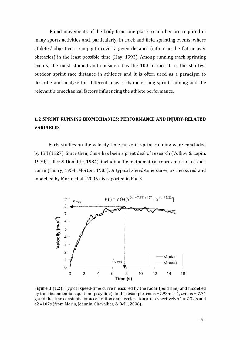
curve (Henry, 1954; Morton, 1985). A typical speed-time curve, as measured and

modelled by Morin et al. (2006), is reported in Fig. 3.

Figure 3 (1.2): Typical speed-time curve measured by the radar (bold line) and modelled by the biexponential equation (gray line). In this example, vmax =7.98m·s–1, tvmax = 7.71 s, and the time constants for acceleration and deceleration are respectively τ1 = 2.32 s and τ2 =107s (from Morin, Jeannin, Chevallier, & Belli, 2006).

- 7 -

Although no general consensus has still been reached by the scientific

community, as well as by track and field coaches, about the number and type of

phases in which a 100 m sprint race should be divided (Jones, Bezodis, &

Thompson, 2009), in the present review four different phases will be considered:

the block-start, the acceleration or pick-up phase, the maintenance and the final

deceleration. There are many factors that affect the duration of each of theses

phases. Internal or personal factors, such as motivation, technique, fitness and

fatigue, as well as external aspects, like strength and direction of wind, air

temperature, and texture or hardness of the track surface (Nigg & Yeadon, 1987;

Stafilidis & Arampatzis, 2007). Their time-duration is, therefore, highly variable

even when considering multiple races of the same athlete and should not be used

as a criterion in the identification of different phases. From Jones et al., (2009), the

most used criterion appears to be the effectiveness of the coaching activity, in

terms of giving to the athletes the necessary level of specificity in the instruction

and feedback. In this respect, the start phase is defined as ranging from when the

athlete obtained a “Set” position in the blocks to the point when the front foot

broke contact with the block. The acceleration/pick-up phase is defined as being

from when the athlete’s front foot left the block to the point when he/she attained

an upright sprinting position. The maintenance phase is seen as the phase in which

the athlete is able to maintain his/her velocity almost constant. Finally, the

deceleration phase is defined as the remainder of the race; that is, from when the

athlete’s velocity starts to decrease to when the finishing line is crossed (Mero,

Komi, & Gregor, 1992).

In the following sections, the execution technique, the pattern of muscular

activation (electromyography – EMG) as well as the main kinematic and kinetic

variables for each of the four identified phases will be discussed.

1.2.1 Block start phase

The block start phase refers to the time when the sprinter is in contact with

the starting blocks. Blocks have been regularly used in track competitions under

the International Amateur Athletic Federation (IAAF) rules since 1948, the year of

London Olympic Games.

- 8 -

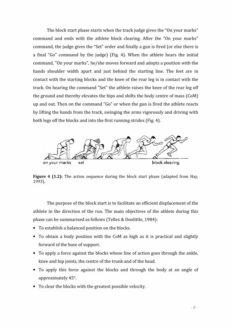
The block start phase starts when the track judge gives the “On your marks”

command and ends with the athlete block clearing. After the “On your marks”

command, the judge gives the “Set” order and finally a gun is fired (or else there is

a final “Go” command by the judge) (Fig. 4). When the athlete hears the initial

command, "On your marks", he/she moves forward and adopts a position with the

hands shoulder width apart and just behind the starting line. The feet are in

contact with the starting blocks and the knee of the rear leg is in contact with the

track. On hearing the command "Set" the athlete raises the knee of the rear leg off

the ground and thereby elevates the hips and shifts the body centre of mass (CoM)

up and out. Then on the command "Go" or when the gun is fired the athlete reacts

by lifting the hands from the track, swinging the arms vigorously and driving with

both legs off the blocks and into the first running strides (Fig. 4).

Figure 4 (1.2): The action sequence during the block start phase (adapted from Hay, 1993).

The purpose of the block start is to facilitate an efficient displacement of the

athlete in the direction of the run. The main objectives of the athlete during this

phase can be summarised as follows (Tellez & Doolittle, 1984):

• To establish a balanced position on the blocks.

• To obtain a body position with the CoM as high as it is practical and slightly

forward of the base of support.

• To apply a force against the blocks whose line of action goes through the ankle,

knee and hip joints, the centre of the trunk and of the head.

• To apply this force against the blocks and through the body at an angle of

approximately 45°.

• To clear the blocks with the greatest possible velocity.

- 9 -

EMG activity

The first aspect to be considered when analysing the block start phase is the

reaction time. It has been defined as the time that elapses between the sound of the

starter’s gun and the moment the athlete is able to exert a certain pressure against

the starting blocks. Reaction time measurement currently includes the time that it

takes for the sound of the gun to reach the athlete, the time it takes for the athlete

to react to the gunshot and the mechanical delay of measurements inherent in the

starting blocks.

An attempt has been made to separate premotor time and motor time

components in the block start phase (Mero & Komi, 1990). The former is defined

as the time from the gun signal until the onset of EMG activity in skeletal muscle.

Motor time is the delay between the onset of electrical activity and force

production by the muscles. EMG results (Mero & Komi, 1990) showed that total

reaction time can be effectively divided into premotor and motor time. However,

electrical activity in some muscles started to increase after total reaction time as a

result of the multi-joint nature of the sprint start movement. It is clear that, after

the gun signal, leg extensor muscles must contribute maximally to the production

of force and ultimately to the running velocity. The faster the electrical activity

begins in every muscle, the faster the athlete can be in maximising the

neuromuscular performance. For improving the start action, it is desirable that all

extensor muscles are activated before any force can be detected against the blocks.

Mero and Komi (1990) used a force threshold of 10% from the maximal

horizontal force production as a measure of reaction time. Total reaction time was

on average 120 ms, which was the minimal reaction time for a valid start in the

Rome World Championships in 1987. In fact, no definitive study exists which could

be used to establish a minimum reaction time to define a false start. For

comparison of reaction times to be used, uniform conditions for measurement

must be established.

The main conclusions regarding reaction time during the block start phase

are (Moravec et al., 1988):

1. In identical events the average reaction times of women are longer than those

of men;

2. Reaction times grow in proportion to the length of race distance;

- 10 -

3. Reaction time does not correlate with the performance levels, thus meaning

that other parameters, as acceleration or maximum speed, may be more

important than reaction time to final race performance.

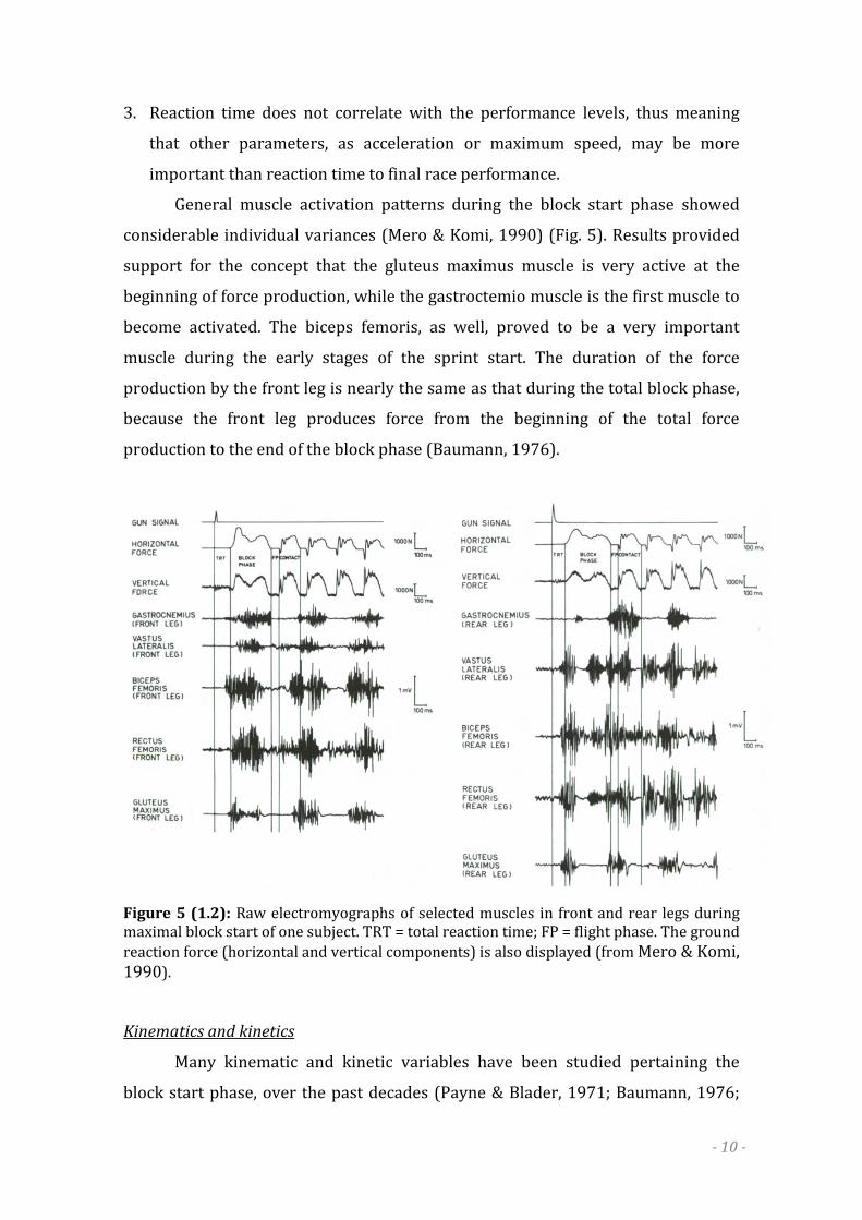
General muscle activation patterns during the block start phase showed

considerable individual variances (Mero & Komi, 1990) (Fig. 5). Results provided

support for the concept that the gluteus maximus muscle is very active at the

beginning of force production, while the gastroctemio muscle is the first muscle to

become activated. The biceps femoris, as well, proved to be a very important

muscle during the early stages of the sprint start. The duration of the force

production by the front leg is nearly the same as that during the total block phase,

because the front leg produces force from the beginning of the total force

production to the end of the block phase (Baumann, 1976).

Figure 5 (1.2): Raw electromyographs of selected muscles in front and rear legs during maximal block start of one subject. TRT = total reaction time; FP = flight phase. The ground reaction force (horizontal and vertical components) is also displayed (from Mero & Komi, 1990).

Kinematics and kinetics

Many kinematic and kinetic variables have been studied pertaining the

block start phase, over the past decades (Payne & Blader, 1971; Baumann, 1976;

- 11 -

Mero, Luhtanen, & Komi, 1983; Cappozzo, Gazzani, & Massacesi, 1989; Schot &

Knutzen, 1992; Fortier, Basset, Mbourou, Faverial, & Teasdale, 2005; Čoh, et al.,

2006; Slawinski, Bonnefoy, & Levêque, 2010; Slawinski et al., 2010). Different

biomechanical variables were obtained and were shown to contribute to a fast

start technique (Harland & Steele, 1997). In the following section, the main results

about biomechanical variables are discussed.

• Inter-block distance: a medium block spacing (as opposed to the bunched or the

elongated one), combined with the hips raised high in the set position, was

theorised to enable sprinters to utilise more completely an extensor reflex of

the muscle groups relevant to sprint starting (Schot & Knutzen, 1992).

Furthermore, the medium starting position produced the fastest acceleration

than enables both a powerful and quick recovery of the rear lower extremity

(Čoh, et al., 2006).

• Block inclination: sprint start performance was shown to improve when

decreasing block inclination. This improvement was attributed to an increased

contribution of the medial gastrocnemius muscle during the eccentric and

concentric phases of calf muscle contraction due to an earlier onset. This

increased contribution appeared to be the result of progressive lengthening of

the soleus and gastrocnemius muscles in the set position as the front block

inclination decreased. Therefore, during the subsequent stretch-shorten cycle,

force production was improved, more effectively providing and elastic

contribution to the speed of muscle shortening (Mero, & Komi, 1990).

• Trunk and knee alignment during the “Set” position: an optimal “Set” position

was shown to exist for highly skilled sprinters irrespective of variations in body

structure. In particular, the stronger the sprinter, the more acute the joint

angles can become. That is, stronger sprinters can use a greater range of joint

extension to gain greater velocity when leaving the blocks (Mero, Luhtanen, &

Komi, 1983; Slawinski, Bonnefoy, & Levêque, 2010). Knee angles during the

“Set” position for elite and non-elite athletes are reported in Tab. 1.

• Hip joint alignment during the “Set” position: hip joint angles in the “Set”

position have been found to significantly differ between good and average

sprinters. In particular, skilled athletes reported lower joint angle values both

for the front and the rear legs (41 and 80 deg respectively, against 52 and 89

- 12 -

deg for average athletes) (Mero, Luhtanen, & Komi, 1983; Slawinski, Bonnefoy,

& Levêque, 2010). These findings suggested that more skilled sprinters placed

their hip extensors muscles on a greater stretch than their less skilled

counterparts.

• CoM position during the “Set” position: positioning the CoM as close as possible

to the start line in the antero-posterior direction was suggested to be important

in creating a good start, as it contributes to reach a position of maximum

instability and it moves the athlete prospectively closer to the finish line, thus

reducing the distance the sprinter must accomplish (Slawinski, Bonnefoy, &

Levêque, 2010). However, too pronounced forward trunk lean in the “Set”

position has to be avoided, as it excessively loads the hands (Tellez & Doolittle,

1984).

Table 1 (1.2): Front and rear knee angles for elite and well-trained sprinters during the “Set” position. The antero-posterior (XCM) and vertical (VCM) components of the CoM position with respect to the start line, together with the antero-posterior position of the shoulders (Xshoulder: midpoint of the line joining the right and the left acromions) are also provided (from Slawinski, Bonnefoy, & Levêque, 2010).

• Block time, velocity and acceleration: block time is defined as the time from the

beginning of force production, with either foot, to the point where no further

force production occurs against the blocks (i.e. block clearing) (Mero, Luhtanen,

& Komi, 1983). From published data (Harland & Steele, 1997), it appears that

more skilled sprinters exhibited shorter block times compared with their less

skilled counterparts. As concerns resultant velocity and acceleration of the

sprinter at loss of foot contact with the block (usually referred to as block or

leaving velocity and acceleration), it is well documented how the ability of an

athlete to leave the blocks at a high velocity generally increases with an increase

in his/her force application on the blocks (Baumann, 1976; Cousins & Dyson,

- 13 -

2004; Mero & Komi, 1990; Slawinski, Bonnefoy, & Levêque, 2010; Čoh, et al.,

2006).

• Peak-force production: faster sprinters have been characterised as being

capable of more adequate propulsion on the rear block during their starts

compared with slower sprinters (Slawinski, Bonnefoy, & Levêque, 2010).

Moreover, skilled sprinters generally apply lower peak force on the rear block

compared to the front block, with the rear block forces being exerted more

rapidly. Fig. 6 reported the force time-curves measured on the rear and front

blocks during the sprint start of a middle-level athlete (Payne & Blader, 1971).

Figure 6 (1.2): Resultant forces measured on the front (ant.) and on the rear (post.) starting blocks, as well as measured on both blocks (total) (adapted from Payne & Blader, 1971).

• Direction of force application: it has been claimed that a good start is

characterised by the exertion of high forces in the horizontal direction

(Baumann, 1976). The angle between the horizontal and the line joining the

CoM to the front toe at the loss of front contact has been reported to range from

32 to 42 deg for skilled sprinters (Mero, Luhtanen, & Komi, 1983). Angles of

force application relative to the horizontal have been reported to vary form 43

deg at loss of block contact to 50 deg at toe-off of the first step (Mero, Luhtanen,

& Komi, 1983).

- 14 -

• Force impulse: impulse incorporates both block force and block time and it is

representative of the average amount of force serving to propel the sprinter and

the time over which this force acts. For skilled sprinters horizontal and vertical

impulses have been reported to range from 233 to 234 Ns and 172 to 231 Ns,

respectively (Mero, Luhtanen, & Komi, 1983; Slawinski, Bonnefoy, & Levêque,

2010). Baumann et al. (1976) also reported that faster sprinters were able to

exert a greater impulse in the horizontal direction (263 Ns) than less skilled

sprinters (214 Ns). As block time was not significantly different between these

groups, the greater impulse exhibited by the elite sprinters was created by a

greater average force production. Similar results have been reported recently

by Slawinski et al. (2010).

1.2.2 Acceleration or pick-up phase

After the block clearing, the runner accelerates by increasing stride length

and stride rate. The pick-up phase ranges from the block clearing to the instant of

time in which the athlete attains an upright sprinting position. Its length is about

30 to 50 m in top sprinters during a 100 m race (Volkov & Lapin, 1979; Moravec et

al., 1988). Two key aspects have been identified in the acceleration phase: arm

action and leg extension (Jones, et al., 2009). As concerns the arm action, Thomson

et al. (2009) identified how previous research (Hinrichs, Cavenagh, & Williams,

1987; Mann, Kotmel, & Herman, 2008) documented the arms’ balancing function in

relation to the motion of the legs while sprinting. Nevertheless, up to now, no

general consensus has been displayed about the amount of elbow and shoulder

flexion and extension and no work seems to have specifically analysed the action of

the arms within the pick-up phase. Leg extension refers to the hip and knee joints

being fully extended prior to the athlete taking-off from each step in order to

maximise the force exerted onto the running track. With this respect, it is

necessary for both legs to have the same behaviour, symmetrical but alternate

(Collier, 2002; Hunter, et al., 2004b). Two more aspects have been reported to be

important during the acceleration phase: first contact times: Coh and Tomazin

(2006) noted that contact phases become shorter and flight phases longer as the

athlete progresses from the starting blocks; second the athlete’s posture: due to

the development of running velocity and the subsequent dynamic changes in

- 15 -

running technique, the athletes’ ability to maintain their dynamic posture as

opposed to the static posture of the sprint start appears to be crucial (Jones, et al.,

2009).

EMG activity

Integrated EMG activity during acceleration has been reported by Mero and

Peltola (1989). In that study two male sprinters ran a 100 m simulated race and, in

the acceleration phase, there was a 4.8% higher maximal integrated EMG activity

during contact than in the maximum constant speed phase. This may imply that

neural activation of sprinters achieves its maximum in the acceleration phase.


The main kinematic and kinetic parameters which have been investigated

during the pick-up phases are hereafter discussed.

• Stance and flight phase duration: mean stance times during the acceleration

phase for elite male sprinters have been shown to range from 0.160 s to 0.194 s

for the first ground contact out of the blocks (Atwater, 1982; Mero & Komi,

1990; Čoh, et al., 2006), and from 0.150 to 0.181 s for the second ground contact

(Atwater, 1982; Čoh, et al., 2006). Flight phases are characterised by lower

durations: from 0.06 to 0.07 s for the first flight and from 0.044 to 0.090 s for

the second flight phase (Atwater, 1982; Čoh, et al., 2006). Conversely, after the

first steps, stance times tend to decrease while accelerating, and flight times to

increase (Zernicke & Whiting, 2000).

• Step length: this is defined as the distance between the first contact point of one

foot to the first contact point of the controlateral foot (differently to “stride

length”, which is the distance between the first contact point of one foot to the

first contact point of the same foot, like for example: right-left-right foot

contacts). Increasing the length of the first step out of the blocks has been

advocated as part of an optimal start (Čoh, et al., 2006). Nevertheless, anterior

braking forces associated with the CoM being ahead of the first ground contact

point were not significantly higher that that created with shorter steps (Schot &

Knutzen, 1992). Moreover, an overly long first step may retard progress of the

- 16 -

sprinter. It has also been shown how the degree of forward lean in the “Set”

position had a varying effect on first step length (Schot & Knutzen, 1992). Tab. 2

reports the step length, as well as the stance and flight times for the first ten

steps of an elite sprinter during the acceleration phase (Čoh, et al., 2006).

Table 2 (1.2): Step length and ground contact and flight times of a professional sprinter during the first ten steps of the acceleration phase (from Čoh, et al., 2006).

- 17 -

• Center of gravity (CoG) position: once the sprinter has started to leave the

blocks, his/her task is to prepare for the subsequent ground contacts that

he/she will make to assume maximal sprint velocity. If the horizontal position of

the first foot to contact the ground after block clearing is posterior to the CoG

along the antero-posterior direction, the sprinter is immediately able to

maximize horizontal force production. Coh and Tomazin (2006) identified the

position of the foot contact as being crucial to the successful execution of the

pick-up phase, specifically minimizing braking forces during the first step.

Indeed, the position of the CoG with respect to the first contact point on the

ground changes during the first few strides. At the beginning of the first two

stance phases, it is ahead of the foot-ground contact point. By the beginning of

the third stance phase, the CoG is already behind the contact point (Mero,

Luhtanen, & Komi, 1983; Slawinski, Bonnefoy, & Levêque, 2010).

• CoM vertical displacement: during the initial ground contact phases following

block clearance, the CoM falls vertically. This vertical displacement reduces the

step rate because of increasing ground contact time and, in turn, reduces the

running velocity (Mero, Luhtanen, & Komi, 1983). Elite sprinters have been

found to exhibit a reduced CoM negative vertical displacement (0.017 ± 0.016

m) during the eccentric phase of the first stance phase compared with slower

sprinters (0.027 ± 0.014 m).

• CoM horizontal velocity: Fig. 7 reports the time-curve of the CoM horizontal

velocity of elite and well-trained sprinters during the first two steps of the

acceleration phase (Slawinski, Bonnefoy, & Levêque, 2010). Similarly, Mero et

al. (1983) reported a mean horizontal velocity of the CoM of 5.7 m·s-1 at toe-off

of the second post-block step for skilled male sprinters.

• Trunk alignment: it has been reported to be approximately 45 deg relative to

the horizontal at loss of contact with the front block (Atwater, 1982; Van

Coppenolle, et al., 1990; Slawinski, Bonnefoy, & Levêque, 2010). As concerns the

trunk orientation during the pick-up phase, however, no general consensus on

the best technique has been reached yet and no work seems to have specifically

analysed such variables within this phase.

- 18 -

Figure 7 (1.2): Evolution of the CoM horizontal velocity of elite and well-trained athletes during the pushing phase and the first two steps of the acceleration phase (from Slawinski, Bonnefoy, & Levêque, 2010).

• Force production: despite the forward position of the CoG with respect to the

first ground-contact point, a negative horizontal force is observed during the

first step, probably caused by the leg moving forwards (Schot & Knutzen, 1992).

This suggests that in sprint running, all stance phases are characterised by

braking and propulsive components of the ground reaction force (GRF) (Hunter,

et al., 2005), although the ratios are different according to the race phase. In

particular, average horizontal forces in the first portion of the race are

considerably larger (526 N) with respect to their braking counterparts (153 N)

(Mero, Komi, & Gregor, 1992). Interestingly, Mero et al. (1992) reported that the

horizontal propulsive force exerted during the first step after block clearing was

46% greater than the same force generated during contact at maximum

velocity. This result highlights the need for the athlete to use a high level of

concentric strength during the acceleration phase.

1.2.3 Maintenance phase

Professional track and field coaches describe a good running technique as

the sum of four crucial aspects. First, the ability of the athlete in maintaining a

relatively high CoM, with a slight anterior tilt of the pelvis during the maintenance

phase of the race. Second, the needs of performing a wide hip flexion during each

- 19 -

flight phase, trying to reach what coaches call “the high hip position” (Collier,

2002). Third, the importance of arm action, with the athlete swinging the arms

exclusively in the progression plane, not across the body and with the elbow angle

maintained close to 90 deg of flexion. The movements of both arms should be the

same, although opposite in direction and they should be corresponding and

complementary (Čoh, et al., 2006; Jones, et al., 2009). During the maintenance

phase, the arms should work as ‘balancing factor’, by providing lift and promoting

a more constant horizontal velocity for the runner (Hinrichs, Cavenagh, &

Williams, 1987; Jones, et al., 2009). Finally, shoulder, neck and facial muscles

should be relaxed once reached the upright position and full speed (Jones, et al.,

2009).

EMG activity

Running requires a complex sequencing of body muscle activation. EMG

activity has generally been found to increase with increased running speed (Mero,

Komi, & Gregor, 1992). In the propulsion phase, EMG activity is markedly lower

than during the braking phase. This may be partly related to increase recoil of

elastic energy during the propulsion phase (Cavagna, et al., 1971). An example of

muscle activation pattern during maximal speed running is presented in Fig. 8.

There is high activity in the leg musculature before contact (Mero & Komi, 1987),

as at the beginning of the contact phase, large impact forces occur. It is important,

therefore, that the leg extensors muscles are highly activated and stiff prior to as

well as at the moment of impact. Energy is transferred by the elastic elements of

the musculo-tendinous complex from the braking to the propulsion phase, and

utilisation of such elastic properties has been shown to be important in increasing

explosive force production during contact (Cavagna, et al., 1971; Hunter, et al.,

2005).

- 20 -

Figure 8 (1.2): Raw electromyographs of selected muscles during stride at maximal speed of one subject. Ground reaction forces measured by a force platform are also reported (from Mero, Komi, & Gregor, 1992).

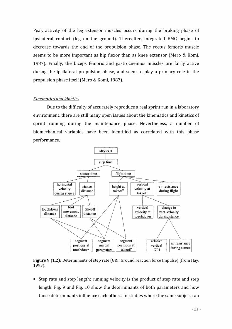
- 21 -

Peak activity of the leg extensor muscles occurs during the braking phase of

ipsilateral contact (leg on the ground). Thereafter, integrated EMG begins to

decrease towards the end of the propulsion phase. The rectus femoris muscle

seems to be more important as hip flexor than as knee extensor (Mero & Komi,

1987). Finally, the biceps femoris and gastrocnemius muscles are fairly active

during the ipsilateral propulsion phase, and seem to play a primary role in the

propulsion phase itself (Mero & Komi, 1987).


Due to the difficulty of accurately reproduce a real sprint run in a laboratory

environment, there are still many open issues about the kinematics and kinetics of

sprint running during the maintenance phase. Nevertheless, a number of

biomechanical variables have been identified as correlated with this phase

performance.

Figure 9 (1.2): Determinants of step rate (GRI: Ground reaction force Impulse) (from Hay, 1993).

• Step rate and step length: running velocity is the product of step rate and step

length. Fig. 9 and Fig. 10 show the determinants of both parameters and how

those determinants influence each others. In studies where the same subject ran

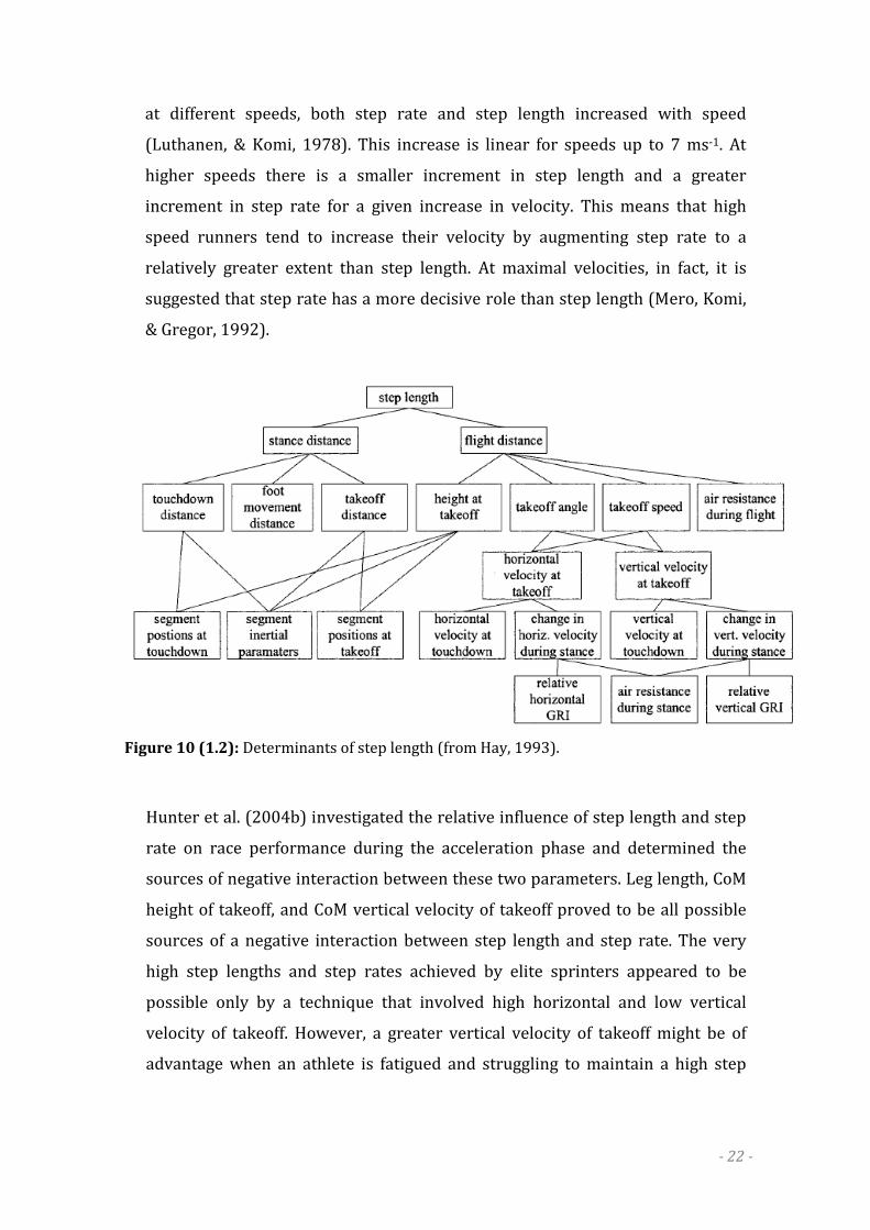
- 22 -

at different speeds, both step rate and step length increased with speed

(Luthanen, & Komi, 1978). This increase is linear for speeds up to 7 ms-1. At

higher speeds there is a smaller increment in step length and a greater

increment in step rate for a given increase in velocity. This means that high

speed runners tend to increase their velocity by augmenting step rate to a

relatively greater extent than step length. At maximal velocities, in fact, it is

suggested that step rate has a more decisive role than step length (Mero, Komi,

& Gregor, 1992).

Figure 10 (1.2): Determinants of step length (from Hay, 1993).

Hunter et al. (2004b) investigated the relative influence of step length and step

rate on race performance during the acceleration phase and determined the

sources of negative interaction between these two parameters. Leg length, CoM

height of takeoff, and CoM vertical velocity of takeoff proved to be all possible

sources of a negative interaction between step length and step rate. The very

high step lengths and step rates achieved by elite sprinters appeared to be

possible only by a technique that involved high horizontal and low vertical

velocity of takeoff. However, a greater vertical velocity of takeoff might be of

advantage when an athlete is fatigued and struggling to maintain a high step

- 23 -

rate. Mean step rate and step length values showed to be 4.26 samples per

second and 1.91 m respectively (Hunter, et al., 2004b).

• Stance and flight times: stance time has been reported to decrease significantly

as running velocity increases (Luthanen, & Komi, 1978), while flight time has

the opposite behaviour. In the maintenance phase flight time ranges from

approximately 0.120 to 0.140 s (Moravec et al., 1988; Hobara et al., 2009). In

Fig. 11, stance and flight times of an elite sprinter performing a 100 m run are

plotted against time. The relevant decreasing and increasing pattern of the two

parameters is visible. Times were obtained by using a high-speed camera

(Bergamini E., unpublished personal observations).

Figure 11 (1.2): Stance (solid line) and flight (dashed line) duration time-curve during a 100 m sprint run of an elite sprinter (Bergamini E., unpublished personal observations).

• Vertical displacement of the CoM: vertical peak-to-peak displacement of the

CoM within the step duration has been shown to decrease with increased

running speed (Cavagna, et al., 1971; Luthanen, & Komi, 1978). Mero et al.

(1992) observed vertical displacements of 0.047, 0.050 and 0.062 m for “good”,

“average” and “low level” male sprinters, respectively. Similar results were

found by Hobara et al. (2009).

• CoM velocity: a number of studies found that at constant speed there is a

decrease in the CoM horizontal velocity following initial foot contact. Then,

- 24 -

during the propulsion phase, the CoM velocity increases. Cavenagh and

Lafortune (1980) found a decrease of 0.18 m·s-1 in running velocity during the

braking phase at 4.47 ms-1, which was followed by an increase of 0.27 m·s-1

during the propulsion phase. Velocity at toe-off was greater than that at touch-

down. Probably due to the air resistance, during the flight phase the horizontal

velocity of the CoM was found to decrease.

Figure 12 (1.2): GRF impulses are shown as areas under the horizontal and vertical GRF curves. p (green) is the propulsive impulse, b (red) is the braking impulse. Propulsive impulse was based on horizontal positive force data during stance, and braking impulse was based on horizontal negative force data during stance. Horizontal impulse was calculated as propulsive impulse minus the absolute value of braking impulse. v (grey) is the area under the vertical GRF curve. When horizontal, braking, propulsive, and vertical impulses are expressed relative to body mass, they reflect the change in velocity of the center of mass (ignoring the effects of wind resistance) during the respective periods and in the respective directions (adapted from Zernicke & Whiting, 2000, and from Hunter, et al., 2005).

• Force production: as during the previously analysed phases of the sprint run,

force production has a key role during the maintenance phase as well. It has

been reported that faster top running speeds are achieved with greater GRFs,

rather than with rapid leg movements (Weyand, Sternlight, Bellizzi, & Wright,

2000). However, it has also been reported that large GRFs as well as high

vertical and horizontal propulsive impulses are involved in stress fractures and

knee-related injuries (Ferber, Kingma, Bruijn, & van Dieen, 2002; Grimston,

Nigg, Fisher, & Ajemian, 1994). The ability of the sprinter to reduce the braking

horizontal forces and to maximise the propulsion forces is crucial for the race

- 25 -

performance (Hunter, et al., 2005). The braking horizontal force and braking

time should be very small to avoid loss of velocity during the impact phase.

Significant correlations were found between the average net resultant force in

the propulsion phase and velocity, as well as between the propulsive force and

the step length. Fig. 12 shows typical horizontal and vertical GRF curves, with

relevant force impulses, for a well-trained sprinter (Hunter, et al., 2005).

Figure 13 (1.2): Spring-mass model using in running to estimate vertical stiffness. The leg spring is compressed during the first half of the stance phase and rebounds during the second half. Maximal vertical displacement of the CoM during ground contact is represented by ΔyC (from Hobara, et al., 2010).

• Stiffness: The concept of stiffness has its origin in physics, as part of Hooke’s

Law. Objects that obey this law are deformable bodies which store and return

elastic energy. Hooke’s Law, defined as F=k·Δy, states that the force (F) required

to deform a material is related to a proportionality constant (k) and the distance

(y) the material is deformed, provided that its shape is not permanently

changed. The proportionality constant, k, is referred to as the spring constant,

and it describes the stiffness of an ideal spring and mass system. The leg is often

modelled as a spring supporting the mass of the body (Fig. 13). Lower extremity

stiffness was proved to be an important and sensitive factor in musculoskeletal

performance (Latash & Zatsiorsky, 1993; Butler, et al., 2003; Brughelli & Cronin,

2008). It appears, indeed, that increased stiffness is beneficial to performance.

At the same time, too little or too much stiffness may increase the risk of

musculoskeletal injury (Butler, et al., 2003). Although there is not a general

consensus about the effect of increased or decreased stiffness on the risk of

injuries, there is some evidence that increased stiffness may be related to bony

- 26 -

injuries and decreased stiffness may be associated with soft tissue injuries

(Burr, Martin, Schaffler, & Radin, 1985; Grimston, Nigg, Fisher, & Ajemian, 1994;

Williams, McClay, & Hamill, 2001; Williams, Davis, Scholz, Hamill, & Buchanan,

2004). It appears to exists, however, an optimal amount of stiffness that allows

for injury-free performance (Butler, et al., 2003). Moreover, it has been

suggested that stiffness can be modified in response to the external

environment or verbal cues (Hewett, Stroupe, Nance, & Noyes, 1996; Smith, &

Watanatada, 2002).

1.2.4 Deceleration phase

Concerning the deceleration phase technique, no particular or specific

aspects have been underlined in the literature. Athletes’ aim and instruction is to

limit as much as possible the speed decrease. This is particularly true in the 200

and 400 m races, where the athlete’s endurance characteristics and anaerobic

metabolism are crucial.

Very few studies focused on the deceleration phase of sprint running from

both a physiological and biomechanical point of view. Recent progress as concerns

technology and methodology will hopefully contribute in enriching the literature

about physiological and biomechanical variables which influence and determine

this phase performance.

EMG activity

EMG activity pattern during the deceleration phase was found to be similar

with respect to that in the maintenance phase (Mero & Peltola, 1989). The average

maximal activity of the muscles during the deceleration phase decreased of 6.8%

with respect to that estimated during the maintenance phase of a simulated 100 m

race.


The deceleration phase is characterised by a decrease of velocity and by a

slight increase in the stance times, and, in turn, a slight decrease in the flight times.

In short sprint running events (especially in the 100 m race), the deceleration

- 27 -

phase is usually visible on the time-velocity curve. The loss of velocity from the

peak during a 100 m race ranges from 0.9 to 7% (Moravec et al., 1988). Step rate

decreases, and step length slightly increases during deceleration (Moravec et al.,

1988; Mero & Peltola, 1989). The CoM vertical displacement was also found to

increase during this phase (Moravec et al., 1988; Mero & Peltola, 1989). No

research data are available concerning the force production and the GRF patterns

during the deceleration phase.

1.3 METHODS FOR SPRINT RUNNING ANALYSIS

This section was written on the basis of a recent review article by Higginson, 2009, on

methods currently used for running gait evaluation. The author’s work is gratefully

acknowledged.

The remarkable increase in the number of recreational and competitive

runners in recent years has obvious implications to professionals such as

clinicians, physical therapists, and coaches who offer services aimed at the

evaluation and rehabilitation of running-related injuries and performance

enhancement strategies. Recent technological advancements now facilitate a

greater range of individuals able to provide these services. With this increased

demand comes an increase in the need to be knowledgeable of the technology

currently available to provide these services.

Many tools have been developed to assist in the assessment of running gait.

These include the more traditional motion capture systems used to describe

motion of the body, force plates that quantify the forces acting on the body, and

electromyography (EMG) used to estimate the level of muscle activity during

motion.

More recently, smaller portable sensors have been developed and

successfully used to measure running gait parameters. These include

accelerometers, electrogoniometers, gyroscopes, and in-sole pressure sensors.

These tools have been successfully used to investigate shoe (Verdejo & Mills, 2004;

Butler, Davis, & Hamill, 2006; Clinghan, Arnold, Drew, Cochrane, & Abboud, 2008;

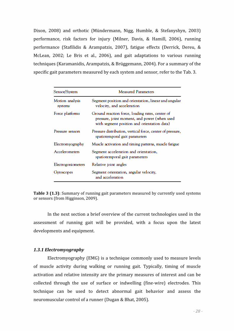
- 28 -

Dixon, 2008) and orthotic (Mündermann, Nigg, Humble, & Stefanyshyn, 2003)

performance, risk factors for injury (Milner, Davis, & Hamill, 2006), running

performance (Stafilidis & Arampatzis, 2007), fatigue effects (Derrick, Dereu, &

McLean, 2002; Le Bris et al., 2006), and gait adaptations to various running

techniques (Karamanidis, Arampatzis, & Brüggemann, 2004). For a summary of the

specific gait parameters measured by each system and sensor, refer to the Tab. 3.

Table 3 (1.3): Summary of running gait parameters measured by currently used systems or sensors (from Higginson, 2009). In the next section a brief overview of the current technologies used in the

assessment of running gait will be provided, with a focus upon the latest

developments and equipment.

1.3.1 Electromyography

Electromyography (EMG) is a technique commonly used to measure levels

of muscle activity during walking or running gait. Typically, timing of muscle

activation and relative intensity are the primary measures of interest and can be

collected through the use of surface or indwelling (fine-wire) electrodes. This

technique can be used to detect abnormal gait behavior and assess the

neuromuscular control of a runner (Dugan & Bhat, 2005).

- 29 -

Normal muscle activation during the stride and stance phases of running

(Cavenagh, 1990; Novacheck, 1998) and sprinting (Mero, et al., 1992) have been

reported (see also § 1.2), as well as how muscle activation and timing patterns are

influenced by changes in walking and running speeds (Cappellini, Ivanenko,

Poppele, & Lacquaniti, 2006). In addition to providing information about muscle

activation levels and timing, the frequency content of the EMG signal can be

analyzed to determine relative muscle fatigue (Wakeling, Pascual, Nigg, & von

Tscharner, 2001), which may be used in the early detection of potential running

injuries. There are also data to suggest that EMG parameters may be a more

sensitive measure than force measures in explaining differences in shoe/orthotic

comfort ratings (Mündermann, et al., 2003).

EMG parameters have been found to be highly reproducible between step

cycles when compared across different running techniques (running velocity and

stride frequency), but tend to be less reproducible when compared across

individual muscles, with distal leg muscles showing more reproducibility than

proximal leg muscles during running (Karamanidis, et al., 2004). Depending upon

the particular muscle of interest, this information may influence selection of gait

analysis protocols by decreasing (or increasing) the number of stride cycles

needing to be analyzed.

One major drawback of older EMG systems is that data were transmitted via

cable, potentially limiting the motion of the subject. Newer systems incorporate

technology that allow for the data to be transmitted wirelessly or stored in a data

logger worn by the subject, vastly increasing the functionality of these systems.

Other limitations include crosstalk between muscles and electrical noise from

external sources (Harris, & Wertsch, 1994). The incorporation of in-line

preamplification devices has greatly reduced ambient noise in the underlying

myographic signal, allowing for greater signal-to-noise ratio. Although selection of

appropriate signal processing and normalization techniques, selection of muscle

onset-offset determination algorithms, and data interpretation are a quite intricate

task to inexperienced operators, many current systems are designed to

accommodate various levels of user proficiency.

- 30 -

1.3.2 Motion analysis (Stereophotogrammetry)

The most common method for collecting information about position and

orientation of body segments in two- or three-dimensional space is the use of

motion capture technology (often referred to as stereophotogrammetry), in which

markers are affixed to the subject and tracked throughout the motion of interest.

These systems typically use passive markers that reflect ambient or infrared light.

Through manual or automatic digitization techniques, the coordinate location

(two- or three-dimensional) of the markers can be determined. From these

position data, the velocity and acceleration can then be calculated by taking the

time derivative of the position and velocity, respectively.

Limitations inherent in both optical systems include the need of skilled

operators and the fact that they can be prohibitively expensive, have a relatively

small capture volume, and require a controlled environment in which to operate

(Sabatini, Martelloni, Scapellato, & Cavallo, 2005). Moreover, even when the motor

task of interest can be performed and analysed in a human movement laboratory,

sports motor acts are particularly problematic, being characterized by high

accelerations and forces. The movement of the soft tissues, and in turn of the skin-

mounted markers, relative to the underlying bones (soft tissue artefact - STA)

appears to be one of the major sources of error in the estimation of kinematic and,

particularly, kinetic parameters in the analysis of sports techniques (de Leva &

Cappozzo, 2006). In this respect, there is a need for research in the development of

new methodologies specifically designed for sports applications.

Edge detection technology recently has shown promise in allowing gait

parameters to be quantified directly from video sources alone, allowing the same

information to be extracted as that from marker-based systems, without the

associated limitations or need for markers.

As concerns the use of treadmills, although they are often used in the

analysis of walking and running gait to overcome issues surrounding small capture

volumes, their use is believed to induce gait adaptations, such as increased time in

stance phase, that normally would not be observed in over-ground running (Dugan

& Bhat, 2005). These changes appear to be speed dependent (Nigg, De Boer, &

Fisher, 1995). Moreover, sprint running can be hardly reproduced on treadmills.

- 31 -

To overcome problems related to the small capture volume, the use of new small

and portable technologies seems to be effectively ideal.

1.3.3 Force plates

Force plates are commonly used to measure contact forces between foot

and ground (ground reaction force – GRF). This information can be used to

quantify impact forces, loading rates, as well as propulsive and breaking forces,

and to track changes in the center of pressure (CoP) over time.

Because of their relatively small size, however, they impose constraints on

foot placement, which may result in subjects adopting a “targeting” strategy while

running, altering natural gait mechanics (Paolini, Della Croce, Riley, Newton, &

Casey Kerrigan, 2007). This targeting strategy can lead to increased step length

variability (Wearing, Urry, & Smeathers, 2000) and often results in exclusion of the

trial (Milner, Ferber, Pollard, Hamill, & Davis, 2006), resulting in prolonged data

collection periods and subject fatigue. Although the influence of targeting shows

little effect upon GRFs during walking gait (Wearing, et al., 2000), greater approach

velocities associated with running and larger changes in relative stride length to

contact the force platform may result in more significant differences observed in

GRFs at these higher speeds.

Recently, the development of instrumented treadmills have allowed for the

quick collection of GRFs over repeated gait cycles, allowing for highly controlled

gait speed, while eliminating potential error introduced by targeting strategies.

One of the major drawbacks of these systems, however, is that treadmills using

force plates beneath the belt can be susceptible to noise because of friction of the

belt moving over the plate. Moreover, as above mentioned, sprint running can be

hardly reproduced on treadmills.

1.3.4 Pressure sensors

The use of in-shoe pressure sensors provides a lightweight, portable, and

easy-to-use alternative in which to analyze running gait. Unlike force platforms,

they are capable of quantifying the distribution of force over the plantar surface of

the foot, providing more detailed information on the loading of the foot during gait

- 32 -

than force measures alone. Because this device is placed in the shoe, the loads

acting on the foot surface can be measured directly, as opposed to the force acting

on the bottom of the shoe with a standard force platform (Dixon, 2008). For this

reason, in-shoe pressure sensors are commonly used to quantify the effect of shoe

design upon foot loading and have been used to compare loading of the foot

between similar shoe types (Clinghan, et al., 2008) and between shoes of different

midsole designs (Dixon, 2008), as well as changes in the impact absorbing

capabilities of a shoe over repeated impact cycles (Verdejo & Mills, 2004).

In-shoe pressure sensors also provide the ability to measure vertical forces

experienced by the foot during prolonged running (Karamanidis, et al., 2004) and

detect typical gait parameters required for gait analysis, such as heel strike and

toe-off needed to define the stance phase of gait (Catalfamo, Moser, Ghoussayni, &

Ewins, 2008). Although force platforms are considered to be the gold standard

method by which these measurements typically are collected, as mentioned

previously, they are limited in the number of steps that can be sampled and

typically their use is restricted to a laboratory setting. In-shoe pressure sensors

give the researcher or clinician the flexibility to collect data from repeated foot

strikes in an environment that facilitates normal running gait.

Plantar loading parameters obtained from in-shoe pressure sensors have

shown high reliability across multiple trials of the same subject, with low

variability between steps (Murphy, Beynnon, Michelson, & Vacek, 2005), and are

repeatable between testing days (Putti, Arnold, Cochrane, & Abboud, 2007).

Analysis of GRF parameters indicates that these measures are reliable, over a

range of running speeds and stride frequencies (Karamanidis, et al., 2004), also

when collected using pressure sensors. However, comparison of the two most

popular in-shoe pressure measurement systems indicates that the accuracy and

precision of these systems may be sensitive to the levels of pressure applied,

calibration procedure, duration of pressure application, and insole age of use

(Hsiao, Guan, & Weatherly, 2002).

1.3.5 Accelerometers

The use of body-fixed sensors such as accelerometers are rapidly becoming

a viable alternative to more traditional gait analysis techniques for use in the

- 33 -

assessment of human motion. Accelerometers are inertial sensors that provide a

direct measurement of acceleration along single or multiple axes, effectively

reducing the error associated with differentiation of displacement and velocity

data derived from sources such as motion capture systems.

Accelerometer-based systems have been used successfully to quantify the

shock experienced by the lower extremity during walking and running (Lafortune,

Henning, & Valiant, 1995; Butler, et al., 2006; Milner, Davis, et al., 2006), evaluate

the effect of footwear (Butler, et al., 2006) and insoles (O'Leary, Vorpahl, &

Heiderscheit, 2008) upon tibial shock during running, evaluate shock attenuation

between body segments during running (Mercer, Bates, Dufek, & Hreljac, 2003),

and investigate the effects of fatigue upon running gait patterns (Le Bris, et al.,

2006).

Perhaps the most appealing advantage is the ability of accelerometers to be

used in the estimation of spatio-temporal gait parameters (Sabatini, et al., 2005),

which until recently required the use of a force plate, motion analysis systems, or

footswitches. As addressed in previous sections, a primary limitation of

stereophotogrammetric systems and force plates in the analysis of running gait is

their limited ability to measure successive strides. Because of their light weight

and portability, accelerometers are capable of recording data that can be collected

continuously over many stride cycles for a prolonged period of time. This

technology has been used effectively to detect alterations in running patterns after

the onset of fatigue in middle-distance runners while running on a track, without

altering the running patterns of the runner (Le Bris, et al., 2006).

Although mechanical testing has confirmed the validity and reliability of

accelerometers in the measurement of accelerations within the frequency and

amplitude range of human body motion (Bouten, Koekkoek, Verduin, Kodde, &

Janssen, 1997), evidence indicates that they are sensitive to the site and method of

attachment, with skin-mounted accelerometers resulting in significantly greater

peak accelerations than bone mounted accelerometers (Lafortune, 1991).

Moreover, direct comparison of axial acceleration of the tibia during running found

that the disparity in results between attachment methods is largely subject-

dependent (Lafortune, et al., 1995). Another drawback of these sensors is that the

acceleration signal is affected by a fluctuating offset (bias) and random white

- 34 -

noise, which may jeopardise the result of the numerical integration process

necessary when velocity or displacement has to be estimated (Woodman, 2007).

1.3.6 Gyroscopes

Gyroscopes are miniature angular rate sensors that can be attached to

individual body segments, providing a direct measure of segment angular velocity.

This sensing technology is an inexpensive alternative to motion analysis systems

(Mayagoitia, Nene, & Veltink, 2002), and methods recently have been developed to

calculate spatio-temporal gait parameters based upon the angular velocity

measures provided by these sensors (Aminian, Najafi, Büla, Leyvraz, & Robert,

2002; Sabatini, et al., 2005). Little measurement error is entailed in estimating

these parameters, in comparison with measurements based on foot pressure

sensors (Aminian, et al., 2002).

In addition to allowing the direct measurement of segmental angular

velocity and calculation of spatio-temporal gait parameters, other benefits of using

gyroscopes include their small size and portability, lower power requirement

(Wong, Wong, & Lo, 2007), and insensitivity to gravitation influence (Sabatini, et

al., 2005). However, as with accelerometers, signal integrity is compromised by

unwanted sensor motion resulting from poor fixation or site selection and from the

bias and random white noise. When integrating the angular velocity signal in order

to estimate the angular displacement, therefore, drift errors can be crucial.

Gyroscopes and accelerometers utility can be further enhanced through the

concurrent use of the two sensors. Sensor fusion theory, borrowed from the

aerospace field, has been applied for estimating sensor orientation, with

accelerometers used for compensating the drift which affects the angular

displacement obtained by numerical integration of noisy gyroscope signals, by

using gravity as an absolute reference direction. The latter assembly is commonly

referred to as inertial measurement units (IMU) (further details are reported in §

3.1.2). When combined with rate gyroscopes, accelerometers have been found to

produce joint angle, angular velocity, and angular acceleration similar to that

derived from motion capture systems under dynamic conditions (Mayagoitia, et al.,

2002), and have been used effectively to estimate walking speed and surface

inclination angles (Sabatini, et al., 2005).

- 35 -

1.3.7 Electrogoniometers

Electrogoniometers allow for the direct measurement of joint angles during

continuous dynamic activities. They offer a simple, affordable alternative to motion

capture systems and allow joint angle data to be collected and viewed

instantaneously. The end blocks of the electrogoniometers typically are affixed to

the skin on either side of the joint axis of rotation using double-sided adhesive

tape, as specified by the manufacturer. This method has been found to result in

excessive sensor motion (Rowe, Myles, Hillman, & Hazelwood, 2001), which

potentially could be magnified during the high-speed changes in joint angle

commonly experienced during running. This unwanted sensor motion can be

effectively reduced through the use of additional adhesive tape (Piriyaprasarth,

Morris, Winter, & Bialocerkowski, 2008) or application of pre-wrap and athletic

tape (Dierick, Penta, Renaut, & Detrembleur, 2004). For prolonged periods of data

collection, special suits have been fabricated, which facilitates attachment of the

electrogoniometers using hook and loop fasteners (Pierre et al., 2006). Failure to

prevent sensor motion and improper alignment of the sensor during the

application procedure has been found to be the greatest potential contributor to

measurement error (Rowe, Myles, Hillman, & Hazelwood, 2001; Wong, et al., 2007;

Piriyaprasarth, et al., 2008).

Measurement error from electrogoniometers has been shown to be as small

as 0.04 degrees (Piriyaprasarth, et al., 2008) and has been validated using both

human (Rowe, Myles, Hillman, & Hazelwood, 2001) and mechanical

(Piriyaprasarth, et al., 2008) testing protocols, with results comparable to those

obtained using motion capture systems (Rowe, Myles, Hillman, & Hazelwood,

2001). Although studies have shown inter- and intra-tester reliability to be

relatively high, it has been suggested that the same tester be used when possible to

ensure the highest repeatability (Piriyaprasarth, et al., 2008). When applied

correctly, electrogoniometers have proven to be highly accurate and highly

sensitive for detecting changes in joint angles over time, providing a simple, small,

portable, and affordable alternative to motion capture systems (Rowe, Myles,

Hillman, & Hazelwood, 2001).

- 36 -

1.4 THEORETICAL BACKGROUND: DISCUSSION

In the last decades, due to the increase in running popularity, biomechanical

variables influencing sprint running performance have been widely studied. In

particular, the block start phase together with the first steps of the acceleration

phase have been performed and analysed both in traditional human movement

analysis laboratory and on instrumented tracks. The evaluation of the maintenance

phase, however, requires the use of treadmills, thus inducing running technique

adaptations that would not be observed in in-field running. This is particularly true

at high speeds.

The lack of portability and the small acquisition volume characterising

traditional laboratory-based instrumentations used for the analysis of human

movement, therefore, still represent the main limitation to in-field evaluation of

sprint running. Thanks to recent technological advances accelerometers,

electrogoniometers, gyroscopes, inertial measurement units and in-shoe pressure

sensors have been made available. Combined with wireless technology and/or

data loggers, they provide an affordable, lightweight alternative to in-field running

analysis, allowing data collection over prolonged periods of time in almost any

environment. Investing resources in the development and validation of methods

and protocols that exploit the use of such technologies, appears, therefore, fully

appropriate.

On the other hand, only very few studies focuses on determining definitive


measures and injury in sprint running. The main result concerns the relationship

between the amount of forces applied to the lower extremities and the incidence of

knee injuries. Being the forces and accelerations involved in sports motor acts

considerably higher with respect to those implicated in clinical contexts, the

development of methods specifically designed for the estimation of internal and

external forces in sports applications is, therefore, desirable.

- 37 -

CHAPTER 2

AIM OF THE THESIS

- 38 -

The present work is part of a co-tutoring PhD program developed by the

University of Bologna, the Locomotor Apparatus Bioengineering LABoratory

(LabLAB) of the University of Rome “Foro Italico” and the Laboratoire de

Biomécanique (LBM) of the Arts et Métiers ParisTech of Paris, France.

The general purpose of the present thesis is to contribute overcoming the

main limitations concerning the biomechanical analysis of sports motor tasks

focusing, in particular, on sprint running evaluation. To this aim, two

complementary approaches have been adopted:

• LOW RESOLUTION APPROACH: the necessity of performing in-field athlete

evaluation without influencing or constraining athletes’ activities will be coped

by exploring the use of wearable inertial measurement units during sprint

running. Relevant biomechanical variables affecting sprint running performance

will be estimated.

• HIGH RESOLUTION APPROACH: the lack of methods specifically designed for

sports applications will be coped by focusing on constraint-based knee joint

models commonly used to enhance the accuracy of joint kinetic estimates, being

the latter particularly crucial in sports injury prevention. To further improve

such models, subject-specific non-rigid constraints for the knee joint will be

defined.

Note: The term “Resolution” refers to the level of detail relative to the specific

framework of analysis. Hence, the Low Resolution Approach entails a global

assessment of the performance by using inertial sensors and a less detailed analysis is

necessary. Conversely, the High Resolution Approach, focusing on the internal forces

and joint kinematics, entails a more detailed observation.

- 39 -

CHAPTER 3

LOW RESOLUTION APPROACH

- 40 -

• V. Camomilla, G. Vannozzi, P. Picerno, E. Bergamini – “Wearable inertial sensors: sport

biomechanics meets performance evaluation”. In: Capranica, L. and Meeusen, R., Intensive

Programme on Sport Performance: A Lifespan Challenge, eds. Routledge, Abingdom, UK.

• E. Bergamini, P. Picerno, V. Camomilla, H. Pillet, A. Cappozzo – “Estimate of temporal

parameters during sprint running by trunk inertial sensing: in field validation”, XXIX

Conference of the International Society of Biomechanics in Sports, June 2011, Porto,

Portugal.

• E. Bergamini, P. Guillon, H. Pillet, V. Camomilla, W. Skalli, A. Cappozzo – “The trunk

orientation during sprint start estimated using a single inertial sensor”, 28th Conference of

the International Society of Biomechanics in Sports, July 2010, Marquette, Michigan (US).

• I. Masci, E. Bergamini, G. Vannozzi, N. Getchell, A. Cappozzo – “Quantitative assessment of

locomotor skills development in childhood: the running paradigm”, 7th Annual

Biomechanics Research Symposium, May 2010, Newark, Delaware (US).

• E. Bergamini, P. Picerno, M. Grassi, V. Camomilla and A. Cappozzo – “Spatio-temporal

parameters and instantaneous velocity of sprint running using a wearable inertial sensing

unit”, 27th Conference of the International Society of Biomechanics in Sports, August 2009,

Limerick (Ireland).

• E. Bergamini, P. Picerno, M. Grassi, V. Camomilla and A. Cappozzo – “Estimate of

performance correlated parameters in non steady-state sprint running using a wearable

inertial measurement unit”, 10th Congresso SIAMOC, October 2009, Alghero (Italy).

- 41 -

ABSTRACT

Athlete’s performance evaluation is one of the main issues of coaching, as

well as of sports biomechanical analysis. An optimised performance is obtained

when accurate, useful, and timely feedback about athlete proficiency is provided.

To this aim, the main goal of sport biomechanists is to provide information to

coaches and athletes about sports skill technique.

As the majority of sports motor acts are hardly repeatable in laboratory

environments, in-field evaluation of the athlete performance, without influencing

or constraining athletes’ activities, is now becoming mandatory in order to provide

coaches with reliable and realistic information. Sprint running is not an exception.

Thanks to their portability and weightlessness, inertial measurement units

allow for data collection during unconstrained continuous movement over

prolonged periods of time. Accelerometer and gyroscope signals measured by

these sensors, however, are affected by two main sources of errors: an unstable

drift that accumulates when numerical integration is performed and the effects of

soft tissue wobbling relative to the underlying bones.

Three studies will be presented aiming at estimating reliable performance-

related parameters by using inertial sensors and at developing methods able to

reduce the effects of the above mentioned sources of errors. In particular, the

trunk inclination and angular velocity, as well as the instantaneous horizontal

velocity and displacement of a point approximating the center of mass will be

provided during in-lab sprint running. The stride and stance durations will be

estimated on-the-field during the maintenance phase.

The fixation of the sensor proved to be a crucial aspect in reducing soft tissue

oscillations. The use of memory foam materials and of ad-hoc elastic belt appears

effective. Reducing the integration interval and cyclically determining the initial

conditions of the acceleration integration process proved to yield reliable

instantaneous velocity as well as spatio-temporal parameters.

KEYWORDS: Performance evaluation; Sprint running; Sprint start; Inertial

sensors; Spatio-temporal parameters.

- 42 -

3.1 INTRODUCTION

3.1.1 Sports biomechanics and in-field performance evaluation

Athlete’s performance evaluation is one of the main issues of coaching. An

optimised performance is obtained when accurate, useful, and timely feedback

about athlete proficiency is provided. A successful coaching outcome is related to

the ability of coaches and trainers to correctly analyse all the deterministic details

of the performance. In this way, training programs can be organized to specifically

target performance defects. Failure in providing such feedback implies a reduction

of chances of improvement (Carling & Williams, 2005). Therefore, athlete

monitoring, evaluation and training planning should be based on systematic,

objective and reliable approaches to improve data acquisition and information

processing. In this respect, a gap exists between sport science research and

coaching practice (Goldsmith, 2000). The link between research and coaching

practice needs to be reinforced, especially in élite sports, where coaches are

progressively going to incorporate the outcomes of sports science research in their

in-field activity (Williams & Kendall, 2007).

Sport coaches aim naturally at improving athlete’s performance and at

reducing injury risk. These two objectives are also shared by sport biomechanists.

The science of biomechanics is concerned with the forces that act on human body

and the effects these forces produce. Physical education teachers and coaches of

athletic teams, whether they recognise it or not, are likewise concerned with

causes (forces) and effects (movement). In fact, a sport technique can be defined as

the way in which body segments move in relation to each other during a

movement task. Coaches’ ability to teach sport techniques depends largely upon

their understanding of both the effects they are trying to produce and the forces

that cause them. Thus, the main goal of sport biomechanists should be to provide

information to coaches and athletes about sports skill technique that will assist

them in obtaining a good technique, characterised by effective performance (the

purpose of the movement) and decreased risk of injury (distribution of forces in

muscles, bones, and joints so that no part is excessively overloaded). Poor

- 43 -

techniques are characterised by increased risk of injury, even though performance

may be effective, at least for a while.

Sport scientists basically use two approaches to analyse athletes’ technique:

qualitative and quantitative. A qualitative analysis is based on the systematic

observation of the motor task, directly and/or via film or video (Knudson, 2007).

The effectiveness of this approach depends on the operator ability to observe

accurately the task and to know what to look for, i.e. on the operator knowledge

and experience and, in particular, his/her ability to identify the mechanical

requirements of the movement under analysis. Since human observation is

generally not sufficient to provide accurate and objective information, the use of

objective data, specific measuring tools, and correct interpretation and application

of the findings are required to optimise the coaching process. This circumstance

calls, therefore, for the use of quantitative analysis. A quantitative analysis is based

on measurements of the kinematic (displacement, velocity, acceleration) and

kinetic (force, moment, power) variables that determine performance. As regards

the mechanical determinants of performance, relevant assessments have been, so

far, typically constrained into laboratory settings. Laboratory-based

instrumentations are accurate, but the volume of capture is limited and may even

vitiate the execution of the motor task under analysis. Here is where sports

biomechanics fails in providing useful and exploitable information to coaches and

trainers.

A perfect example of the “breakpoint” between sports biomechanics and

performance evaluation is represented by Mr. Pistorius with his emblematic 400 m

race during the 2007 Golden League in Rome. After his brilliant vamp in the last

200 m, a group of researcher was requested (by the International Association of

Athletics Federations, IAAF) to investigate about his sprint performance ability and

determine whether or not he could have had mechanical advantages from his

prostheses. Two groups of researchers performed different mechanical and

physiological tests on Mr. Pistorius. The first expressed its positive opinion

regarding the advantages coming from the prostheses, while the second group

expressed the opposite attitude. This report was then followed by the sentence

emitted by the Court of Arbitration for Sport (Lausanne, May 2008) which stated

“Having viewed the Rome Observations [...] the IAAF's officials must have known that

- 44 -

[...] the results would create a distorted view of Mr. Pistorius' advantages and/or

disadvantages by not considering the effect of the device on the performance of Mr.

Pistorius over the entire race”. In fact, the researchers’ investigation was performed

using lab-based instrumentations and, thus, was limited to few steps. Conversely,

in cases like this, a mechanical characterisation of the motor task must be carried

out for the entire race. The abovementioned circumstance might be overcome

when adequate technological advancements are made available.

Technological advances and improvement of procedures have been and

continue to be an important issue in sport and exercise science (Winter, et al.,

2007). To cope with the fast development of new technological advancements,

sports scientists and coaches are asked to continuously account for new

developments and include them in the everyday assessment of training and

competition. Specifically, technologies used to measure performance are moving

forward and improved methods based on “state of the art” computer technology

and robotic automation are being continually developed and commercialised to

support the pursuit of success in elite sports (Carling, Reilly, & Williams, 2009).

Systems of measurement benefitted of such trend with a progressive device

miniaturisation, increased reliability and cost reduction. Simultaneously, data

processing took advantages of greater calculation power, speed and interactivity.

Last but not least, the development in the use of expert systems such as, for

example, Artificial Neural Networks, as diagnostic tools for evaluating faults in

sports techniques is advocated as promising in the near future (Bartlett, 2006).

Professionals from computer science and engineering fields cooperate with

sports biomechanists and physiologists to define and implement performance

indices that can be used by trainers and coaches during the performance

evaluation exercise. From the same multidisciplinary interaction, further

improvements were attained, such as instrumented sports equipments or portable

systems that use telemetry for data transmission. These ones are particularly

useful for in-field performance evaluation being not bound to laboratory

conditions.

- 45 -

3.1.2 Wearable inertial sensors

An alternative to laboratory based techniques is the use of inertial sensors

that can measure movement-related data without any space limitation and no

cumbersome setup. Their measure is based on the reluctance (inertia) of a portion

of the sensor to accelerate linearly (accelerometer, inertia to linear motion) or

about an axis (gyroscope, inertia to angular motion) as a response to forces and

torques impressed to them, respectively. The vestibular system, located in the

inner ear, is a biological 3D inertial sensor. It can sense angular motion as well as

linear acceleration of the head.

The measured quantities are expressed with respect to a moving reference

frame defined by the sensitive axes of the sensors. The sensitive axis is the axis

along which the acceleration is “sensed” and about which the rotational velocity is

“sensed”. Accelerometers and gyroscopes may become triaxial when three uniaxial

sensors are mounted mutually orthogonal to each other. When a measure of a

global (inertial) reference frame is required, the measure of the direction and of

the intensity of a local magnetic field is also used.

Only recently advances in micro-electro-mechanical systems (MEMS)

technologies have led to the development of a new generation of inertial sensors,

the specifications of which - in terms of encumbrance, robustness, power

consumption, measuring performance and cost - seem to be appropriate for

applications in the biomedical field. Sensor fusion theory, borrowed from the

aerospace field, was applied for estimating sensor orientation: accelerometers are

used for compensating the drift which affects the angular displacement obtained

by numerical integration of noisy gyroscope signals, using gravity as an absolute

reference direction. The latter assembly is commonly referred to as inertial

measurement units (IMU). Sensor fusion algorithms are then enhanced with the

magnetic sense furnished by MEMS magnetometers, using the magnetic North as

an absolute reference direction on the horizontal plane. With the latter assembly,

also known as a magnetic field angular rate gravity (MARG) sensors (Bachmann,

1999), an absolute Earth-fixed reference frame is provided.

Currently, the major disadvantage of MEMS is the reduced performance in

terms of accuracy and bias stability. Signals measured by MEMS sensors are,

indeed, affected by a fluctuating offset (bias) and random white noise. Size and

- 46 -

performance of an inertial sensor seem to be linearly dependent parameters, thus

the smaller the sensor, the lower the performance expected. On the other side,

MEMS technology transforms inertial sensors into body-fixed sensors. MEMS

sensors are highly transportable and do not need any stationary units such as

transmitters, receivers or cameras. All detected signals can be recorded by a

portable data logger, allowing the subject to perform his/her activity in a real

situation. There are no restrictions in the capturing volume and data can be

recorded for long periods of time depending on the performance and capacity of

the data logger. All these features allow mobile and outdoor motion capture. In

addition, these sensors are much cheaper than sonic, magnetic and optical motion

capture systems and present a high ecological validity: being worn by the subject,

they can be used in non-standardized environments and on any surface (for e.g.

grass, sand, balance beam, springboard, etc.). Moreover, little time is needed to set

up the system and a large number of athletes can be evaluated in a short time in

agreement with trainers’ requirement.

For all these reasons, the availability of wearable motion sensors has

opened new perspectives in sport sciences and, in particular, in the field of human

movement analysis. In few years a large number of applications have appeared

both in the literature and on the market. For example, vertical jump performance

has been analysed using triaxial or uniaxial accelerometers either placed on the

ankle (Quagliarella, Sasanelli, Belgiovine, Moretti, & Moretti, 2010) or on the

sacrum (Innocenti, Facchielli, Torti, & Verza, 2006; Palma, Silva, Gamboa & Mil-

Homens, 2008). However, all these assessments suffered from the limits of

accelerometers and did not take advantage of the presence of gyroscopes that

could greatly enhance the evaluation (Mazzà, Iosa, Picerno, & Cappozzo, 2009).

Strength and power measures can contribute in devising methods to

improve power output and to support its transference to athletic performance

(Cronin & Sleivert, 2005). Although it is still debatable whether training at

maximal power improves functional performance, maximal power needs to be

constantly monitored and adjusted. Isokinetic and isometric assessment bear little

resemblance to the accelerative/decelerative motion implicit in limb movement

during resistance training and sporting performance (Cronin & Sleivert, 2005),

- 47 -

while measures performed using inertial sensors seem ideal to perform power

assessment (Jidovtseff, et al., 2006).

Kinetic information derived from acceleration measures gain increased

value when obtained directly on the field. A well fitting example is the system,

constructed by Baca and colleagues, for recording and presenting relevant kinetic

information during on-water and ergometer rowing (Baca, 2006). Similarly, IMUs

have been used as training aid for hammer throw (Otha, Umegaki, Murofushi,

Komine, & Miyaji, 2008), or, on the tennis court, as a tool to perform a motor

strategy analysis, investigating the translational and rotational motion of the swing

(Ahmadi, Rowlands, & James, 2006) or highlighting differences in the forehand

stroke according to aim and direction (Camomilla, Lupi, & Picerno, 2008). Coupling

accelerometers with other monitoring techniques could enhance their potential as

a means to assess performance over the entire course. This approach was used, for

example, by competition rowers to improve performance at national and

international competitions, monitoring impeller velocity (James, Davey, & Rice,

2004). Moreover, foot-ground contact times (Auvinet, et al., 2002; Purcell, et al.,

2005; Lee, Mellifont, & Burkett, 2010; Wixted, et al., 2010), lower leg rotational

kinematics (Channells, et al., 2005), vertical stiffness (Hobara, et al., 2009) and

running gait symmetry (Lee, Sutter, Askew, & Burkett, 2010) have been assessed

using accelerometers on the tibia or on the lower-back trunk during distance and

sprint running.

It must be kept in mind, however, that the extraction of movement-related

information content from the signal derived from MEMS sensor can be strongly

jeopardized by the unstable bias that characterises the signal of such sensors and

by soft tissue vibrations. In the case of sport performance assessment, during the

execution of explosive sport manoeuvres, the former plays a secondary role

compared to the devastating effects of soft tissue vibration. For this reason, prior

to perform any measurement, good practice rules recommend to mitigate this

source of error for the benefit of the further signal processing. Developing

algorithms that can minimise the detrimental effects of these errors, while

transforming this data into well-known parameters suitable for use by coaches and

athletes, remains the main challenge. Novel derivative techniques, pattern

recognition of specific activities, and characterisation of specific phases of the task

- 48 -

can greatly improve sensor data interpretation. This data reduction can lead to

valuable information that can be made available to coaches and trainers directly on

the field and during real scenarios, such as training sessions or race simulations.

- 49 -

3.2 STUDY 1: TRUNK INCLINATION DURING THE SPRINT START USING AN

INERTIAL MEASUREMENT UNIT

Abstract

The execution of the start is crucial in determining the performance during

sprint running. In this respect, trunk inclination is a key element in moving from

the crouch to the upright position. The purpose of this study was to provide

coaches with an instrument able to reliably estimate such parameter in-field. To

this aim, the accuracy of an inertial measurement unit (IMU) in estimating its

rotation about a local axis and the relationship between this rotation and trunk

inclination in the progression plane were assessed during block start and pick-up

phases.

Sprint starts were performed by five sprinters and data provided by an IMU

positioned on the trunk at L2 level were compared to reference

stereophotogrammetric measurements. An attachment that limited soft tissue

oscillations and Kalman filtering were used to reduce errors. The trunk was

modeled as a rigid segment joining the midpoint between C7 and the posterior

superior iliac spines.

The accuracy of the IMU in estimating its orientation about a local axis was

high both in terms of curve similarity (correlation r>0.99) and of bias (lower than

1 deg). Similar results were obtained concerning the relationship between the IMU

estimates and the trunk inclination in the progression plane (r>0.99; bias lower

than 4 deg). Results open a promising scenario for an accurate in-field use of IMUs

for sprint start performance assessment.

Keywords: Inertial sensor; Kalman filter; Performance indicator; Sprint start;

Biomechanics.

- 50 -

3.2.1 Introduction

The proper execution of the sprint start is crucial in determining the

performance during the 100, 200 and 400 m track sprint runs (Harland & Steele,

1997; Ostarello, 2001; Čoh, et al., 2006). The main outcome of the sprint start is to

move from a static crouched position to a cyclic upright one, by generating

sufficient upward vertical velocity and, at the same time, by creating maximal

forward horizontal velocity to improve the sprint performance. To reach high

horizontal velocities, sprinters have to exert high horizontal forces through the

blocks in a short time period (Harland & Steele, 1997; Čoh, et al., 1998; Kraan, van

Veen, Snijders, & Storm, 2001).

Different parameters were obtained and were shown to be correlated with

the athlete time at 20 m, divided in the block start phase, ranging from when the

athlete obtains the “on your marks” position to block clearing, and pick-up phase,

ranging from the block clearing to the instant of time in which the athlete attains

an upright sprinting position:

• the relative position and the inclination of the blocks (Schot & Knutzen, 1992;

Cousins & Dyson, 2004; Čoh, et al., 2006);

• the vertical and horizontal trajectory and velocity components of the athlete’s

centre of mass (Natta & Breniere, 1997; Cousins & Dyson, 2004; Čoh, et al.,

2006; Kugler & Janshen, 2010);

• the force impulse exerted on the blocks during the block phase (Kugler &

Janshen, 2010; Slawinski, Bonnefoy, & Levêque, 2010);

• the reaction time, i.e. the time from the gun signal to the first detectable change

of pressure on instrumented blocks, and the block time, i.e. the total time the

athlete spends on the blocks, from the first detectable change of pressure to the

front block clearing (Mero, et al., 1992; Fortier, et al., 2005; Čoh, et al., 2006);

• the time between the onset of leg muscle activity and that of force production

(Mero & Komi, 1990).

All these parameters, however, are related entirely or mainly to the lower

part of the body. Only recently, Slawinski et al. (Slawinski, Bonnefoy, Ontanon, et

al., 2010) reported that, since the upper body kinetic energy contributes

significantly to the total body kinetic energy, the coordination between the upper

and the lower part of the body is a key factor in the block start performance. From

- 51 -

coaches’ perspective, it is acknowledged that the upper part of the body is also

important. In fact, expert track and field coaches focus primarily on the inclination

of the trunk in the progression plane described as the line joining the shoulder and

the hip joint centers (Jones, Bezodis, & Thompson, 2009).

Only a few quantitative studies have focused on the trunk during the sprint

start (Mero, Luhtanen, & Komi, 1983; Čoh, et al., 1998; Natta, Decker, & Boisnoir,

2006; Slawinski, Bonnefoy, Ontanon, et al., 2010). Trunk inclination in the

progression plane was analysed during the set position (Mero, Luhtanen, & Komi,

1983; Čoh, et al., 1998; Natta, Decker, & Boisnoir, 2006) and, on a sample of female

athletes, was found to correlate with the athletes’ time to 10 and 20 m from the

starting line (Čoh, et al., 1998). Natta and colleagues (Natta, Decker, & Boisnoir,

2006) reported that the trunk angular velocity, analysed during the block start,

discriminates between high and medium level sprinters. None of these studies

monitored the trunk inclination and angular velocity during both block start and

pick-up phase. Moreover, data acquisition was performed using motion capture or

video analysis technologies, both limited in terms of acquisition volume, post-

processing time, and cost.

As an alternative to video-based techniques, wearable inertial measurement

units (IMUs) have recently gained momentum as a suitable solution for low cost in-

the-field biomechanical analysis of running performance. They provide, without

any space limitation and cumbersome setup, 3D linear acceleration and 3D angular

velocity with respect to a local unit-embedded system of reference. So far, IMUs

have been used to estimate foot-ground contact times (Purcell, et al., 2005) and

lower leg rotational kinematics (Channells, et al., 2005) during sprint, and to

estimate runners’ speed (Vetter, Onillon, & Bertschi, 2009), symmetry between

right and left lower limb (Lee, Sutter, Askew, & Burkett, 2010), and stride, step, or

stance durations during jogging (Lee, Mellifont, & Burkett, 2010) and running

(Auvinet, Gloria, Renault, & Barrey, 2002; Wixted, Billing, & James, 2010). To the

authors’ knowledge, no study has focused on using an IMU to estimate trunk

inclination during the sprint start.

The quality of trunk motion estimates provided by inertial sensors has been

assessed for clinical applications only during daily-life activities or under

controlled flexion-extension, lateral bending and torsion (Lee, 2003; Goodvin,

- 52 -

Park, Huang, & Sakaki, 2006; Plamondon, et al., 2007; Wong, & Wong, 2008; Faber,

Kingma, Bruijn, & van Dieen, 2009). The results of these studies cannot be directly

extended to sprint start, since the quality of the IMU estimates strictly depends on

the amount and variation of acceleration entailed in the analysed motor task for

the following reasons. First, skin-mounted sensors result in significantly greater

peak accelerations than bone mounted sensors (Lafortune, 1991; Forner-Cordero,

et al., 2008) and this is particularly true for movements characterised by high

accelerations and in areas where soft tissues may undergo increased wobbling (Liu

& Nigg, 2000; Pain & Challis, 2006). Second, it is known that the accuracy of sensor

orientation estimate can be improved using adaptive algorithms for weighting the

acceleration or the angular velocity signal (Sabatini, 2006), with the former

prevailing during static or quasi-static phases and the latter during jerked phases,

typical of sprint start. Last but not least, such prevalence of angular velocity signals

entails dealing with the relevant drift which causes errors that accumulate over

time when estimating the angular displacement through numerical integration

(Woodman, 2007).

Within this framework, the purpose of this study was to provide coaches with

an instrument that can be reliably used in the field and that is able to provide

information about the inclination of the trunk, through a three step approach:

1. to minimize problems related to IMU fixing, data fusion, and drift;

2. to assess the accuracy that characterises the estimate of the rotation about a

local axis of an IMU;

3. to quantify the relationship between the latter rotation and the instantaneous

inclination of the trunk in the plane of progression during both the block start

and the pick-up phase.

To these aims, sprint starts were performed in a laboratory. Data provided by

an IMU fixed on the lower part of the trunk were compared to reference

measurements provided by a stereophotogrammetric system.

3.2.2 Materials and methods

Experimental set up and data acquisition

After institutional approval of the protocol, five male sprinters (age:

23.8±0.8 years; body mass: 72.4±3.8 kg; stature: 1.79±0.07 m) were recruited to

- 53 -

take part in the study and gave their written informed consent. The subjects were

currently competing over 100 m or 200 m and their best time for 100 m was

11.35±0.15 s. These times are representative of trained college level athletes.

Each sprinter was asked to perform four starts from the starting blocks. All

sprint runs were performed in an indoor lab (12x9x4m). The blocks were directly

fixed to a wooden tile, which replaced one of the regular floor tiles, and were

individually set by the athletes. The two main body positions during the block start

phase, “on your marks” and “set” positions, and the first three steps of each start

were analysed. To avoid fatigue, a five minutes rest period was given between

trials. Each subject was equipped with an IMU (FreeSense, Sensorize Ltd, Italy)

containing a 3D accelerometer (±6 g of full range) and a 3D gyroscope (±500 deg·s-

1 of full range) providing 3D accelerations and angular velocities with respect to a

local sensor-embedded system of reference coinciding with the geometrical axes of

the IMU case. IMU data, whose sampling frequency was set at 100 frames per

second, were sent via Bluetooth® to a laptop computer and low-pass filtered using

a moving local regression on windows of 40 samples based on weighted linear

least squares and a second degree polynomial model (smooth function with the

loess method, v7.9, MathWorks®, USA). An IMU was positioned with an elastic belt

on the lower back trunk (L2 level). In order to limit the wobbling of muscular and

soft tissue masses (Forner-Cordero, et al., 2008), a memory foam material placed

between the paravertebral muscles and the elastic belt (Fig. 1). The IMU x and y

axes (Fig. 2) were aligned with the spine and with the line joining the posterior

superior iliac spines, respectively.

To validate the use of the IMU, a nine camera stereophotogrammetric

system (Vicon MX3, Oxford, UK) was used. Four retro-reflective markers (LI, LS, RI,

RS) were attached to the IMU to determine the unit orientation in space (Fig. 1).

Ten markers were positioned on the trunk (right and left shoulder, RSHO and

LSHO, spinous process of the 7th Cervical Vertebrae, C7, 10th Thoracic Vertebrae,

T10) and on the pelvis (right and left posterior superior iliac spine, RPSIS and

LPSIS, and anterior superior iliac spine, RASIS and LASIS) (Fig. 1).

- 54 -

Figure 1 (3.2): Markers and IMU placement. Four retro reflective markers (LI, LS, RI, RS) were attached on the IMU. Ten markers were positioned on the trunk: right and left shoulder (RSHO, LSHO), spinous processes of the 7th Cervical Vertebrae (C7), 10th Thoracic Vertebrae (T10), right and left posterior superior (RPSIS, LPSIS), and anterior superior iliac spines (RASIS, LASIS). Further markers were placed to ease the reconstruction and labeling procedure. Indication of the memory foam material location is provided.

Data processing

IMU angular velocity and acceleration were measured in the IMU Technical

reference frame (TIMU). An inertial reference frame was defined in a static phase

preliminary to the acquisition aligning the x-axis of the TIMU with the gravity vector

(IMU Global reference frame – GIMU). The 3 by 3 rotation matrix, which expressed

the orientation of TIMU with respect to GIMU ( IMU

IMU

T

GR

), was then computed (Fig. 2).

To improve the accuracy of the IMU

IMU

T

GR

estimate, a Kalman algorithm

(Kalman, 1960; Jurman, et al., 2007) was designed to automatically identify the

static and non-static phases of the movement and to use a proper combination of

the information provided by the accelerometer and gyroscope sensors. Briefly, the

filter works as follows:

• when the unit does not move or moves at constant velocity, i.e. the norm of the

acceleration vector measured by the unit is below a defined threshold (s), its

inclination relative to the gravitational acceleration is computed through a

quaternion based approach (Favre, Jolles, Siegrist, & Aminian, 2006);

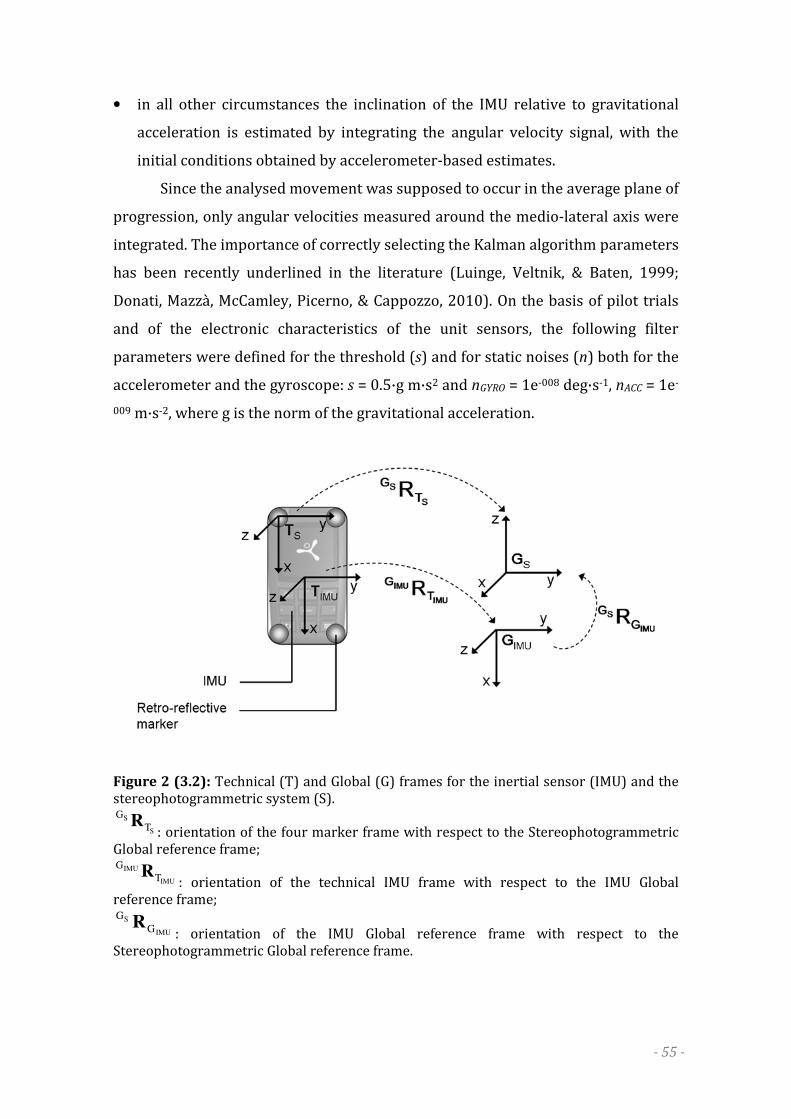
- 55 -

• in all other circumstances the inclination of the IMU relative to gravitational

acceleration is estimated by integrating the angular velocity signal, with the

initial conditions obtained by accelerometer-based estimates.

Since the analysed movement was supposed to occur in the average plane of

progression, only angular velocities measured around the medio-lateral axis were

integrated. The importance of correctly selecting the Kalman algorithm parameters

has been recently underlined in the literature (Luinge, Veltnik, & Baten, 1999;

Donati, Mazzà, McCamley, Picerno, & Cappozzo, 2010). On the basis of pilot trials

and of the electronic characteristics of the unit sensors, the following filter

parameters were defined for the threshold (s) and for static noises (n) both for the

accelerometer and the gyroscope: s = 0.5·g m·s2 and nGYRO = 1e-008 deg·s-1, nACC = 1e-

009 m·s-2, where g is the norm of the gravitational acceleration.

Figure 2 (3.2): Technical (T) and Global (G) frames for the inertial sensor (IMU) and the stereophotogrammetric system (S).

S

S

T

GR

: orientation of the four marker frame with respect to the Stereophotogrammetric Global reference frame;

IMU

IMU

T

GR

: orientation of the technical IMU frame with respect to the IMU Global reference frame;

IMU

S

G

GR

: orientation of the IMU Global reference frame with respect to the Stereophotogrammetric Global reference frame.

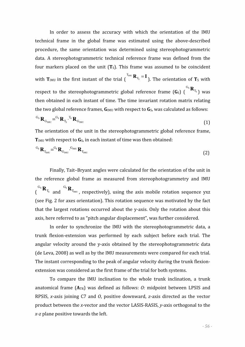
- 56 -

In order to assess the accuracy with which the orientation of the IMU

technical frame in the global frame was estimated using the above-described

procedure, the same orientation was determined using stereophotogrammetric

data. A stereophotogrammetric technical reference frame was defined from the

four markers placed on the unit (TS). This frame was assumed to be coincident

with TIMU in the first instant of the trial (IR =

S

IMU

T

T

). The orientation of TS with

respect to the stereophotogrammetric global reference frame (GS) ( S

S

T

GR

) was

then obtained in each instant of time. The time invariant rotation matrix relating

the two global reference frames, GIMU with respect to GS, was calculated as follows:

IMU

S

S

S

IMU

S

G

T

T

G

G

GRRR ⋅=

(1)

The orientation of the unit in the stereophotogrammetric global reference frame,

TIMU with respect to GS, in each instant of time was then obtained:

IMU

IMU

IMU

S

IMU

S

T

G

G

G

T

GRRR ⋅=

(2)

Finally, Tait–Bryant angles were calculated for the orientation of the unit in

the reference global frame as measured from stereophotogrammetry and IMU

( S

S

T

GR

and IMU

S

T

GR

, respectively), using the axis mobile rotation sequence yxz

(see Fig. 2 for axes orientation). This rotation sequence was motivated by the fact

that the largest rotations occurred about the y-axis. Only the rotation about this

axis, here referred to as “pitch angular displacement”, was further considered.

In order to synchronize the IMU with the stereophotogrammetric data, a

trunk flexion-extension was performed by each subject before each trial. The

angular velocity around the y-axis obtained by the stereophotogrammetric data

(de Leva, 2008) as well as by the IMU measurements were compared for each trial.

The instant corresponding to the peak of angular velocity during the trunk flexion-

extension was considered as the first frame of the trial for both systems.

To compare the IMU inclination to the whole trunk inclination, a trunk

anatomical frame (ATR) was defined as follows: O: midpoint between LPSIS and

RPSIS, x-axis joining C7 and O, positive downward, z-axis directed as the vector

product between the x-vector and the vector LASIS-RASIS, y-axis orthogonal to the

x-z plane positive towards the left.

- 57 -

The pitch angular displacement relative to GS (β) was obtained from the IMU,

IMU

S

T

GR

, from the unit markers, S

S

T

GR

and from the whole trunk, TR

S

A

GR

. Four

phases were identified on the pitch angular displacement (on your marks = OYM,

transition = TNS, set = SET, pick-up = PICK-UP phases) separating static and non-

static phases (Fig. 3). The following parameters were computed for each curve:

• βOYM and βSET: average values during OYM and SET phases, respectively;

• Δβ: difference between βSET and βOYM;

• ωTNS: peak angular velocity during the TNS phase;

• ωPICK-UP: peak angular velocity during the PICK-UP phase.

The offset between the pitch angular displacements calculated using IMU

S

T

GR

and

TR

S

A

GR

was calculated in the OYM position (βOFF).

Figure 3 (3.2): Typical pitch angles (β) for one trial as obtained from the IMU technical frame (solid line), from the stereophotogrammetric technical frame (dotted line) and from the trunk anatomical reference frame (dashed line). The angular displacement parameters estimated for each phase (OYM: on your marks, TNS: transition, SET: set, PICK-UP: pick-up) are indicated: βOYM and βSET: average values of the pitch angular displacement during the OYM and SET positions, respectively; Δβ: peak to peak difference between βSET and βOYM. The pitch angular displacement was considered to be zero when the unit was in a horizontal position; positive angles correspond to clockwise rotations.

- 58 -

Statistical analysis

To assess the accuracy of the parameters provided by the IMU against the

TS reference measurements, as well as the relationship between the information

provided by the IMU and the trunk considered as a rigid segment (ATR), a two steps

statistical analysis was performed.

First, curve similarity was evaluated between pitch angular displacements

obtained from TIMU and TS, for IMU accuracy assessment, and from TIMU and ATR,

for IMU-trunk rotation consistency, computing the root mean square difference

(RMSD) and the Pearson’s product-moment correlation coefficient (r). It has to be

underlined that, when dealing with IMU accuracy, the RMSD between the unit

estimates and reference measurements can be interpreted as root mean square

error. The same coefficients were also assessed for only the PICK-UP phase,

potentially the most affected by inertial factors.

Second, for each computed parameter, the following statistical analysis was

performed:

1. Descriptive statistics (mean±standard deviation);

2. Mean bias analysis: difference between the stereophotogrammetric system

parameters (S) and IMU measurements (IMU);

3. Investigation of the presence of a linear trend between the amount of random

error and the measured values (heteroscedasticity) through inspection of

Bland and Altman plots and correlation analysis (Nevill & Atkinson, 1997).

3.2.3 Results

The comparison of pitch curves, obtained from TIMU and TS when assessing

the accuracy of the IMU, resulted in a low root mean square difference (RMSD) and

a very high correlation (r) during block and pick-up phases (Tab. 1). Similar results

were obtained for IMU-trunk rotation consistency, comparing pitch curves

obtained from TIMU and ATR (Tab. 1).

- 59 -

IMU TR

r 0.994 ± 0.013 0.998 ± 0.002

rPICK-UP 0.995 ± 0.015 0.998 ± 0.001

RMSD [deg] 3 ± 2 3 ± 2

RMSDPICK-UP [deg] 3 ± 3 3 ± 2

Table 1 (3.2): Curve similarity: Mean ± one standard deviation of the Root Mean Square Difference (RMSD) and the correlation coefficient (r) computed to assess unit accuracy (IMU) and IMU-trunk rotation consistency (TR), relative to the whole task and to the PICK-UP phase.

For all pitch parameters, bias was lower than 1 deg, for the IMU accuracy

(biasIMU), and than 4 deg, for IMU-trunk rotation consistency (biasTR). The offset of

the pitch angle between the unit and the trunk reference frame, computed in the

OYM phase, showed a low variability among subjects and trials (βOFF = 18±4 deg).

The peak bias of the angular velocity, during both the TNS and the PICK-UP phases,

was found to be lower than 9 and 6 deg·s-1 for IMU accuracy and IMU-trunk

rotation consistency, respectively (Tab. 2).

TS TIMU ATR TS vs TIMU ATR vs TIMU

biasIMU biasTR

βOYM [deg] -29±6 -29±6 -29±6 1 ± 1 0 ± 1

βSET [deg] 12±6 12±7 9±6 1 ± 1 4 ± 4

Δβ [deg] 43±7 43±8 39±5 1 ± 1 4 ± 4

ωTNS [deg·s-1] 106±19 98±18 93±18 8 ± 4 4 ± 6

ωPICK-UP [deg·s-1] -201±25 -192±29 -198±31 9 ± 6 6 ± 13

Table 2 (3.2): Parameter analysis: Descriptive statistics (mean ± standard deviation) of each estimated parameter and of the errors between the estimates of technical stereophotogrammetric frame (TS), the IMU frame (TIMU), and the anatomical trunk frame (ATR). βOYM and βSET: average values of the pitch angular displacement during the OYM and SET positions, respectively; Δβ: peak to peak difference between βSET and βOYM; ωTNS: peak angular velocity during the TNS phase; ωPICK-UP: peak angular velocity during the PICK-UP phase.

Symmetry of the confidence interval of the bias was observed for all

parameters listed in Tab. 2, during visual inspection of the Bland and Altman plots

entailing that no systematic error was present. No linear trend between the

amount of bias and the measured values was found (average correlation = 0.09).

- 60 -

3.2.4 Discussion

The accuracy of an IMU positioned on the lower part of the trunk in

estimating its rotation about a local axis during sprint start, as well as the

relationship between the IMU estimates and the athletes’ trunk inclination were

assessed. The results show that problems associated with the IMU can be

overcome so that coaches can be provided with an instrument that can be reliably

used in the field to characterise the inclination of the trunk considered as a rigid

body.

The accuracy of the IMU is shown by the high agreement between the IMU

and the reference measures, during the whole trial as well as during the PICK-UP

phase, for both curve similarity and parameter analysis. Such agreement proves

that the main errors entailed in using IMUs to estimate inclination during dynamic

exercises did not have a disruptive effect on the final results. First, the proper

identification of static and non-static phases, as well as the selection of the

weighting on the accelerometer and the gyroscope measurements, are critical to

estimate the unit orientation using Kalman filtering (Sabatini, 2006). The efficacy

of the used filter is attested by the high curve similarity obtained during a

combination of static and non-static phases, as well as during the pick-up phase.

Curve similarity allows hypothesizing that the unit fixing site and method (elastic

belt plus memory foam material placed at L2 level) are a good solution in order to

limit the artefact introduced by soft tissue oscillations. Last but not least, the drift

errors entailed in the numerical integration process of the angular velocity signals

(Woodman, 2007) proved to be negligible, given the short duration of the

integration interval (from the SET end to the upright position there was less than 1

s).

The trunk inclination, considered as a rigid segment, and the IMU

inclination were in high agreement during the whole curve and the PICK-UP phase.

The trunk average peak angular velocity (ATR: ωPICK-UP = 198 ± 31 deg·s-1) agrees

with previous literature results, although slightly higher (186 ± 48 deg·s-1 in Natta

et al., (2006), and about 150 deg·s-1 in Slawinski et al., (2010). This difference can

be explained considering that both studies analysed the task on a real track, where

it is plausible that athletes tended to reach an upright position more gradually with

respect to the athletes tested in the present study, who were forced to complete

- 61 -

the task before reaching the end of the lab. The sensor and the trunk pitch angles

in the OYM phase presented an offset due to a different alignment of the IMU and

the trunk, depending on subjects’ anatomy and due to the athletes’ kyphosis. The

low values of RMSE and the relevant high correlation indicate, consistently

between subjects, that the initial offset does not change during all phases. It could

be speculated that a calibration between the unit and the athlete trunk should not

be necessary, whenever the attention is focused on the variation of the angular

displacement, as it is often the case in coaches’ perspective.

The agreement between the unit and the trunk inclination seems to support

track and field coaches’ approach in considering the trunk as a rigid segment. From

the expert coaches’ perspective, the orientation of the trunk is usually observed

only in the progression plane, as the angular displacement is preponderant in this

plane, and it is considered as a rigid segment (Jones, et al., 2009). Although it is

well known that the trunk has a complex behaviour during the sprint, in the light

of the previous considerations, it is questionable whether a more complex analysis

would be of any use to a coach used to qualitatively observing the task.

In conclusion, the study shows that a single IMU positioned on the lower

back trunk provides reliable angular displacements in the plane of progression

during a sprint start from blocks. Moreover, from these estimates, it is possible to

quantify the inclination of the trunk considered as a rigid segment. The inclination

of the trunk could be particularly helpful for trainers, being one of the key

elements in block start and pick-up performances. Future works, will therefore,

concern the validation of the method in-field, in order to analyse professional

sprinters and all-out sprint starts, exploring, in particular, the correlation between

the estimated parameters and the whole race performance.

- 62 -

3.3 STUDY 2: INSTANTANEOUS VELOCITY AND CENTER OF MASS

DISPLACEMENT OF IN-LAB SPRINT RUNNING USING AN INERTIAL

MEASUREMENT UNIT

Abstract

The biomechanical analysis of sprint running during in-field training

provides valuable information regarding athlete motor strategies, helping in

preventing injuries and achieving higher athletic performance. Wearable inertial

sensing units (IMUs) providing movement-related data without any space

limitation or cumbersome set up can be proficiently used to perform such analysis.

Nevertheless the noise characterizing these sensor signals exacerbates the process

of determining velocity and position by numerical integration of acceleration.

This study aims at compensating these errors by cyclically determining the

initial conditions of the integration process to yield reliable instantaneous velocity

as well as spatio-temporal parameters during sprint running.

Six sprinters performed three in-lab sprint runs, starting from a standing

position. The stance time (ST), and the progression displacement (d) and mean

progression velocity (v) of a point approximating the centre of mass were

estimated and compared with reference data (force platform and

stereophotogrammetric measurements).

Preliminary results showed a high correlation (r > 0.9) between IMU and

reference estimates for each parameter. No statistical differences were found

between IMU and reference for v and ST.

These results proved that the methodology successfully compensate the

numerical integration errors during non steady-state running. Future

developments will concern in-field sprint running experimental sessions.

Keywords: Sprint running; Velocity; Displacement; Inertial sensors; Biomechanics.

- 63 -

3.3.1 Introduction

Field performance analysis of sprint running can be carried out using

several approaches, according to the inquired resolution. Total running time and

step frequency are basic yet very useful information for a global assessment of the

athlete’s performance (Mehrikadze & Tabatschnik, 1982).

Inertial sensors have been used to determine these or similar simple

parameters. Foot-ground contact times (Auvinet, et al., 2002; Purcell, et al., 2005;

Wixted, et al., 2010) and lower leg rotational kinematics (Channells, et al., 2005)

have been assessed using accelerometers on the tibia. Displacement

measurements and running speed have been estimated placing IMUs on the foot

(Fyfe & Gildenhuys, 2004) and, during steady-state running, in a chest-belt (Vetter,

Onillon, & Bertschi, 2009), respectively.

However, when the focus is on performance determinants and limiting

factors, a deeper analysis could be necessary, so that to provide track and field

coaches with detailed information about the athlete’s technique. Stance duration,

step length and center of mass (CoM) instantaneous velocity are key quantities in

such analysis. Theoretically, the numerical integration of the sensor-measured

acceleration yields to the instantaneous velocity and displacement of the segment

where the IMU is attached. In practice, the numerical integration process remains

challenging due to two sources of error. First, accelerometers are characterised by

offset errors that rapidly accumulate over time and yields to unreliable velocity

and displacement (Woodman, 2007). Although in constant speed running, the drift

of the velocity is linear and can be removed with a filtering procedure (Pfau, Witte,

& Wilson, 2005; Pereira, et al., 2008), during non steady-state running, like

sprinting is, this drift is no longer linear. Second, when dealing with explosive

movements, sensor wide oscillations caused by the inertia of soft tissues (de Leva

& Cappozzo, 2006) and by the fixing device (Forner-Cordero, et al., 2008) lead to

sudden velocity increase/decrease that could highly under/overestimate the

actual velocity.

In this pilot work, a methodology for estimating instantaneous velocity and

displacement of a point approximating the CoM from trunk accelerometry during

non steady-state running is illustrated. Low frequency errors are compensated by

reducing the numerical integration interval to the duration of the stance phase and

- 64 -

by predicting the kinematics of the sensor during the flight phase. The initial

conditions of the integration process are, then, cyclically determined.



Six sprinters (five males: age = 27±2 yrs, stature = 1.78±0.07 m, mass =

72±7 kg; one female: age = 27 yrs, stature = 1.65 m, mass = 65 kg) gave their

written consent to participate in this study. After 20 minutes warm up, each

athlete was asked to perform three sprint runs, starting from a standing position.

To avoid fatigue, a 10 minutes rest period was given between trials.

Due to limited laboratory volume (12x9x4m) only the first three steps were

analysed. Subjects were equipped with 39 markers to determine the instantaneous

3D position of the CoM (Plug-in Gait protocol - Davis et al., 1991) using a nine-

cameras stereophotogrammetric system (Vicon Mx, Oxford, UK). Two six-

component force plates (Bertec) were used to measure ground reaction forces at

the second and the third steps.

According to preliminary tests, an IMU (MTx, Xsens, Netherlands) was

positioned using a specifically designed shoulder-belt on the upper back trunk (C7

level). This sensor embedded 3D accelerometer, 3D gyroscope and a

magnetometer. Through the combination of the information provided by these

sensors, the orientation of the IMU relative to the magnetic North and to the

gravity line could be obtained. Stereophotogrammetry, force platforms, and

inertial sensors data were collected simultaneously at 100 samples per second.

Data processing

Before estimating velocity and displacement, accelerations were expressed

with respect to an inertial reference frame (M), aligned with the sprinting direction

(Ma) (Cappozzo, della Croce, Leardini, & Chiari, 2005). Assuming the trunk as a

rigid segment, the acceleration of the IMU was translated along the longitudinal

axis to the mid point between posterior superior iliac spines (midPSIS), closer to

the CoM. Thereafter, the instantaneous progression velocity and displacement

were computed by numerical integration of the acceleration. The integration was

limited to the stance phase only, to avoid the drift typical of the integration

- 65 -

process. During the flight phase, the horizontal kinematics of midPSIS was

predicted using the ballistic law of motion; the velocity at the instant of take-off

was set to the last value of the previously integrated acceleration. This procedure

was reiterated for each step.

Foot contact times were determined using the vertical component of Ma.

Once having identified the highest high-frequency peaks in the time-derivative of

the acceleration signal, the beginning and the end of the flight phase were

determined moving downward through the signal until the acceleration

approached ≅ -9 m·s-2.

The following parameters were estimated over each step: 1) stance time

(STe); 2) CoM progression displacement (de); 3) mean progression velocity (ve)

computed as the arithmetic mean of the instantaneous progression velocity

between two consecutive foot strikes. Reference data were obtained as follows:

STr from force plates (steps 2-3); dr and vr from the CoM trajectory obtained by

stereophotogrammetry. The average percentage difference (e%) between IMU and

reference estimates, referred to as error, was calculated for each parameter.


Statistical analysis was performed using SPSS (version 17.0), with α set to

0.05. Multivariate ANOVA was performed across the three performed trials on the

estimated parameters to establish whether significant differences existed among

trials. Two-tailed paired t-test was performed to establish whether significant

differences existed between methods (reference and estimate). Pearson’s

correlation coefficient was computed on reference and estimated d and v values.

Least significant difference post hoc comparisons with Bonferroni adjustments

were used for multiple comparisons.

3.3.3 Results

The methodology developed in this study yielded to more reliable

instantaneous progression velocity with respect to that obtained by standard

numerical integration of the acceleration (Fig. 1). No differences were found for ST,

d and v values across the three trials (p > 0.05). No differences (p > 0.05) and high

correlation (r = 0.957) were found between the sensor and the reference estimates

- 66 -

of the velocity (ve and vr). Similarly, no differences (p > 0.05) were found between

STe and STr over the first and the second stance phases. Despite statistical

differences were found between de and dr (e% = 10%), a high correlation was

found between these parameters (r = 0.967). Correlation between sensor and

reference estimates for d and v is shown in Fig. 2.

Figure 1 (3.3): Instantaneous progression velocity as obtained by the reference measurements (solid line), computed by numerical integration of the acceleration for the whole duration of the task (dashed line) and with the algorithm proposed in this study (dashed line). Vertical dashed lines identify the flight phases (f1, f2 and f3).

Figure 2 (3.3): Reference and estimated progression displacement and mean velocity of the CM for all the collected trials.

3.3.4 Discussion

The investigation of performance determinants and limiting factors of

sprint running requires the estimate of the linear kinematics of the CoM of the

- 67 -

subject. When the analysis is performed using inertial sensors, the kinematics of

the CoM can be estimated only through assumptions and simplified models. In the

present study, errors introduced by the numerical integration of the acceleration

were compensated by limiting the integration to the stance phase and by

predicting the kinematics of the sensor during the flight phase using the ballistic

law of motion. The initial conditions of the integration process were, then,

cyclically determined. The instantaneous horizontal velocity and displacement of

the CoM were estimated.

Results concerning the reliability of the estimates showed a high agreement

between the sensor and the reference measurements for each estimated

parameters, and a high accuracy for v and ST. Significant differences were found

between reference and IMU estimates only for d. This is probably due to the

double integration process necessary to obtain d from the acceleration. Despite

such differences, the mean error was found to be lower than 10% with respect to

the reference measurements. Moreover, as above mentioned, a high correlation

between reference and IMU d estimates was found (Fig. 2). It has to be noted that d

is strictly related to the athlete’s step length, a very important parameter in

performance assessment which is of great interest for track and field coaches.

However, further research dealing with this correlation is necessary.

Results concerning the estimates of the instantaneous velocity (v) proved

that the drift error entailed in the numerical integration of the acceleration signal

was minimised. The shoulder belt used for the fixation of the IMU, aiming at

reducing the movement of the soft tissues relative to the skeleton with respect to

the pelvic area, appears to be a reasonable compromise between methodological

and practical requirements. Nevertheless, athletes’ arms oscillation during the

acceleration phase was partially disturbed by the underarm stripes. Therefore,

further investigations about the inertial unit fixation have to be performed.

In conclusion, the proposed methodology proved to compensate numerical

integration errors during non steady-state running. The agreement found between

the measured and estimated parameters showed that the methodology is sensitive

to the variations of these parameters. Aside from the encouraging results obtained

in this study, in-field validation of the proposed method is necessary.

- 68 -

3.4 STUDY 3: TEMPORAL PARAMETERS OF IN-FIELD SPRINT RUNNING USING

AN INERTIAL MEASUREMENT UNIT

Abstract

Sprint running temporal parameters are useful information for track and

field coaches. Using wearable inertial measurement units (IMUs) to perform an in-

field analysis of these variables requires being able to temporally locate events

correlated with foot-ground contacts by identifying consistent and repeatable

features on the signal waveforms measured by the IMU. Feature-identification,

however, highly depends on the signal to noise ratio, especially unfavourable

during sprint running analysis because of the explosiveness of the task and of the

oscillations of the IMU relative to the underlying skeleton.

The aim of this study was to identify recognizable and consistent features in

the waveform of the signals supplied by a trunk mounted IMU, or thereof derived,

for the estimation of the stance duration during sprint running.

Eleven subjects (six amateur and five elite athletes) performed three 60 m

sprint runs and data provided by an IMU positioned on the trunk at L2 level were

compared to reference forceplate and high-speed camera measurements. Feature

identification was performed on the magnitude of the acceleration (a) and angular

velocity (ω) vectors and on their 1st ( a& and ω& ) and 2nd ( a&& and ω&& ) wavelet-

mediated derivatives.

Repeatable features were not identified in either a or its derivatives, while

ω was characterized by a consistent positive peak that allows for the identification

of the stride cycle duration. The beginning and end of the stance were identified

from positive and negative peaks on ω&& , consistently across subjects and trials.

Mean errors in the estimate of the stance and stride phase duration were found to

be of the same order than the temporal resolution of the IMU (0.005 s).

Keywords: Sprint running; Contact times; Inertial sensor; Feature-identification;

Biomechanics.

- 69 -

3.4.1 Introduction

Temporal parameters, such as flight and stance duration, are basic yet very

useful information for track and field coaches. The influence on sprint running

performance of these durations and of related parameters, such as stiffness and

ground reaction force impulse, has been widely investigated in the literature

(Butler, Crowell, & Davis, 2003; Hunter, Marshall, & McNair, 2004a; Hunter,

Marshall, & McNair, 2004b; Hunter, Marshall, & McNair, 2005; Morin, Dalleau,

Kyrolainen, Jeannin, & Belli, 2005; Čoh, Tomažin, & Štuhec, 2006; Ito, Ishikawa,

Isolehto, & Komi, 2006; Ciacci, Di Michele, & Merni, 2010).

Commonly, to compute or estimate temporal parameters during sprint

running, force platforms (Hunter, et al., 2004b, 2005), stereophotogrammetric

systems (Ciacci, et al., 2010), optical bars (Čoh, et al., 2006) or video analysis (Ito,

et al., 2006) have been used. The first two instruments, however, allow for the

analysis of few steps, being all limited in terms of acquisition volume. Moreover, as

a real sprint run can not be entirely reproduced in a laboratory, it is necessary to

bring these instruments on the track, which results to be laborious and time-

consuming. Video analysis, which may allow for the analysis of a wider portion of

the track, still requires a non automatic post-processing that might be time-

consuming as well.

As an alternative to the above mentioned instruments, inertial

measurement units (IMUs) have been widely used to measure temporal

parameters, particularly during walking (Jasiewicz et al., 2006; Kavanagh & Menz,

2008; Hanlon & Anderson, 2009). Such parameters have been generally

determined by identifying mechanically-related features in the acceleration and

angular velocity signal waveforms. It is well known, for example, that during

walking, the peak forward acceleration coincides with the instant of foot contact

(Verkerke, Hof, Zijlstra, Ament, & Rakhorst, 2005) or that a repeatable trunk

rotation about the trunk longitudinal axis occurs, during walking as well as during

running, prior to foot contact (Schache, Blanch, Rath, Wrigley, & Bennell, 2002;

Saunders, Schache, Rath, & Hodges, 2005).

Due to their portability and weightlessness, IMUs have recently gained

momentum as a suitable solution for low cost in-the-field biomechanical analysis

of running performance as well. So far, only two studies focused on the estimate of

- 70 -

foot-ground contact times during sprint running using accelerometer-based

systems. Hobara et al. (2009) estimated stance and flight times using a heel-

mounted bi-axial accelerometer, for a model-based estimate of the vertical

stiffness over a 400 m sprint run. The stance durations were measured from the

output waveform of the accelerometer, but no validation was presented nor

previously published by the authors. Purcell et al. (2006) validated with a force

platform the estimates of stance durations based on a shank-mounted tri-axial

accelerometer during the first three steps of the acceleration phase, as well as

during the steady-state phase of a sprint running. However, mounting sensors on

lower legs, aside from requiring two devices, does not provide information on the

body center of mass (CoM) and on trunk kinematics.

These drawbacks may be overcome using a single device on the trunk,

which can be reasonably acceptable by runners. Trunk-mounted devices have been

used to estimate temporal parameters only during distance running (Auvinet,

Gloria, Renault, & Barrey, 2002; Wixted, Billing, & James, 2010). Both authors

concluded, on a qualitative level, that the acceleration signals agreed with the

waveforms of force platforms (Auvinet, et al., 2002) or of in-shoe pressure sensors

(Wixted, et al., 2010), but neither clearly identified mechanically-related features

in the signal waveforms nor provided quantitative information on the accuracy of

their estimates.

Robustness and reliability of these temporal estimates rely on the accurate

and consistent identification of the above-mentioned features within and across

subjects which, in turn, highly depends on the signal to noise ratio. In this respect,

sprint running analysis is more challenging than walking and distance running

because the explosiveness of the task causes greater movements of the IMU

relative to the underlying skeleton (Liu & Nigg, 2000; Pain & Challis, 2006;

Wakeling & Nigg, 2001). As this artefact was shown to be both subject-dependent

(Lafortune, Henning, & Valiant, 1995) and sensitive to the site and method of the

unit attachment (Forner-Cordero et al., 2008; Lafortune, 1991), it may jeopardize

the consistency of the feature identification approach (Higginson, 2009).

The purpose of this study was, therefore, to identify recognizable and

consistent features in the waveform of the signals supplied by a trunk-mounted

IMU, or thereof derived, for the estimation of the stride and stance durations

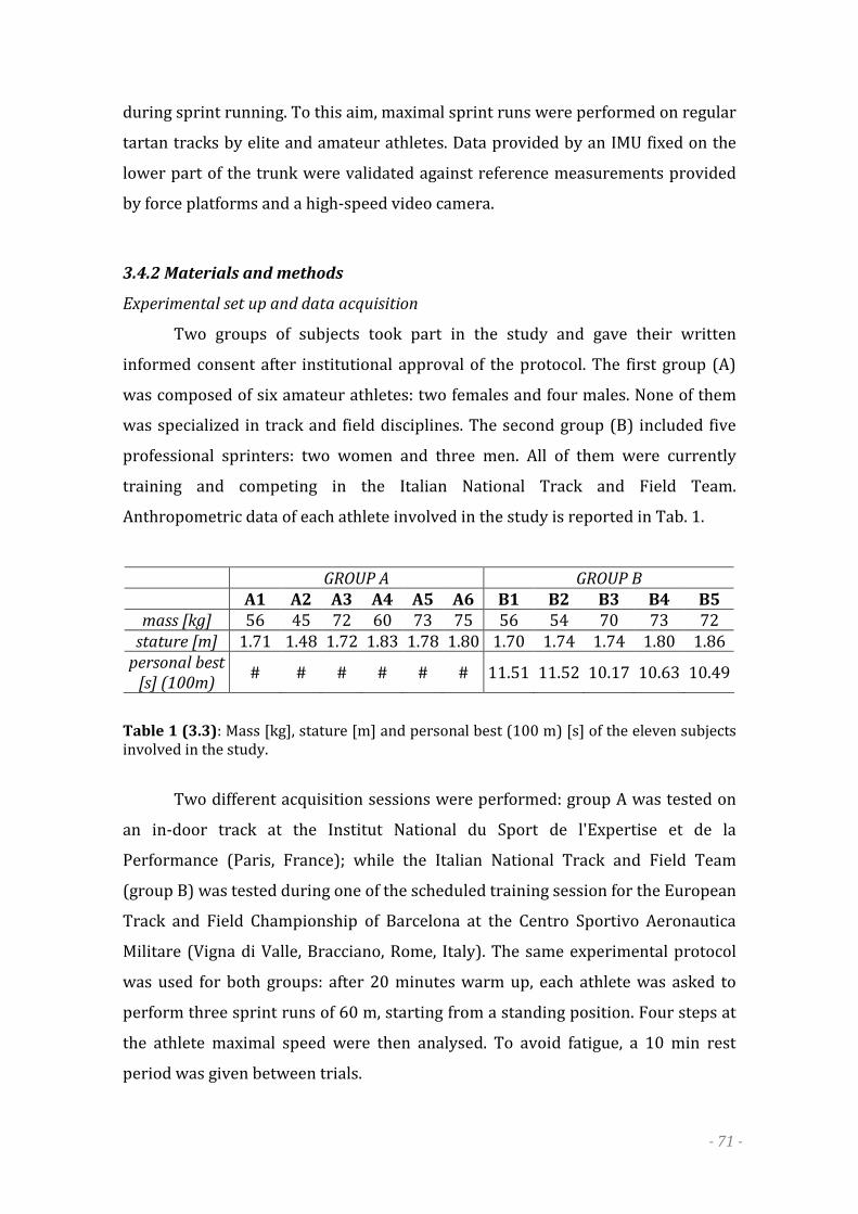
- 71 -

during sprint running. To this aim, maximal sprint runs were performed on regular

tartan tracks by elite and amateur athletes. Data provided by an IMU fixed on the

lower part of the trunk were validated against reference measurements provided

by force platforms and a high-speed video camera.



Two groups of subjects took part in the study and gave their written

informed consent after institutional approval of the protocol. The first group (A)

was composed of six amateur athletes: two females and four males. None of them

was specialized in track and field disciplines. The second group (B) included five

professional sprinters: two women and three men. All of them were currently

training and competing in the Italian National Track and Field Team.

Anthropometric data of each athlete involved in the study is reported in Tab. 1.

GROUP A GROUP B

A1 A2 A3 A4 A5 A6 B1 B2 B3 B4 B5

mass [kg] 56 45 72 60 73 75 56 54 70 73 72 stature [m] 1.71 1.48 1.72 1.83 1.78 1.80 1.70 1.74 1.74 1.80 1.86

personal best

[s] (100m) # # # # # # 11.51 11.52 10.17 10.63 10.49

Table 1 (3.3): Mass [kg], stature [m] and personal best (100 m) [s] of the eleven subjects involved in the study.

Two different acquisition sessions were performed: group A was tested on

an in-door track at the Institut National du Sport de l'Expertise et de la

Performance (Paris, France); while the Italian National Track and Field Team

(group B) was tested during one of the scheduled training session for the European

Track and Field Championship of Barcelona at the Centro Sportivo Aeronautica

Militare (Vigna di Valle, Bracciano, Rome, Italy). The same experimental protocol

was used for both groups: after 20 minutes warm up, each athlete was asked to

perform three sprint runs of 60 m, starting from a standing position. Four steps at

the athlete maximal speed were then analysed. To avoid fatigue, a 10 min rest

period was given between trials.

- 72 -

Each subject was equipped with an IMU (FreeSense, Sensorize Ltd, Italy)

containing a 3D accelerometer (±6 g of full range) and a 3D gyroscope (±500 deg·s-

1 of full range) providing 3D accelerations and angular velocities with respect to a

local sensor-embedded system of reference coinciding with the geometrical axes of

the IMU case. IMU data, whose sampling frequency was set at 200 frames per

second, were sent via Bluetooth® to a laptop computer (MathWorks® v7.9, USA).

Careful attention was paid to the fixation of the IMU to the athletes’ body (Forner-

Cordero, et al., 2008) to limit the unit oscillations relative to the underlying bone.

The IMU was positioned on the lower back trunk (L2 level) with an ad-hoc elastic

belt, not limiting the athlete’s movements. This location was chosen in order to

avoid the low lumbar area, more affected by the wobbling of muscular and soft

tissue masses. To further limit the unit oscillations due to the paravertebral

muscular mass, a memory foam material was placed between the paravertebral

muscles and the unit (see Fig. 1 (3.2), § 3.2.2).

To validate IMU results, two different instruments were used: group A data

were validated using six force platforms (AMTI, USA) directly embedded in the

track and covered with a layer of tartan, not to influence or disturb the athletes

while running. The total platform surface was about 6.6 m length per 0.6 m wide.

Sampling frequency was set at 200 frames per second. To collect at least four steps

on the platform area at the athlete’s maximal speed, the starting line was set at 40

m from the beginning of the first platform. Group B data were validated using a

high-speed video camera (Casio Exilim EX-F1, Japan) whose sampling frequency

was set at 300 frames per second. The camera was positioned at 40 m from the

starting line and registered at least four steps for each athlete. For group A, force

platforms and IMU data were synchronised with a small hammer by hitting the

platform upon which the IMU was positioned. As, above mentioned, data for elite

athletes were collected during an official training session, for practical time

reasons no accurate synchronisation between the camera and the IMU signals was

possible.

Data processing

IMU angular velocity and acceleration were measured in the local IMU

reference frame. As the actual orientation of the unit was not known, the norm of

- 73 -

both the acceleration (a) and the angular velocity (ω) vectors was computed and

further considered. This was done in order to avoid any source of variability which

may arise from different sensor positioning or running technique (particularly as

concerns trunk orientation) (Patterson & Caulfield, 2010).

The first ( a& and ω& ) and second ( a&& and ω&& ) derivatives of a and ω were

calculated using a wavelet-based approach (Jianwen, et al., 2006).

a, a& and a&& , as well as ω, ω& and ω&& signal waveforms of group A were

synchronized with the vertical ground reaction force (GRF), and repeatable

quantifiable events that could be related with the mechanics of the task, such as

maxima, minima, or slopes were identified in correspondence with foot-strike (FS)

and foot-off (FO) instants. Features adequate for automatic detection of FS and FO

were then identified on both group A and B data and, thereafter, used to estimate

stance ( d~

stance) and stride ( d~

stride) durations.

Validation of results thus obtained was performed by comparing the

estimates with reference measurements. Reference dstance and dstride values were

obtained for group A setting a threshold of 10 N on rising edges and of 25 N on

descending edges of the vertical component of the GRF. These thresholds were set

as criteria measures for identifying FS and FO instants respectively (Hunter, et al.,

2005). As concerns group B, a frame by frame video-analysis was performed and

FS and FO instants were visually identified to measure dstance and dstride.


To assess the accuracy of d~

stance and d~

stride the following statistical analysis

was performed separately on group A and group B results:

1. A repeated-measures analysis of variance (ANOVA) was used to verify the

effect of the factors groups, subject and trial on the estimated parameters, both

for the reference and the IMU values.

2. Descriptive statistics (mean ± standard deviation (SD)) of both d~

stance and

d~

stride;

3. Bland and Altman plots, corrected for the effect of repeated measurement error

(Bland & Altman, 2007), were used to assess the agreement between methods

(reference and IMU estimates) with multiple observations (Atkinson & Nevill,

- 74 -

1998). The absence of a linear trend between the amount of random bias and

the measured values (heteroscedasticity) was investigated through inspection

of Bland and Altman plots and correlation exploration (Nevill & Atkinson,

1997).

4. Finally, for each parameter a repeated-measures analysis of variance (ANOVA)

was used to verify the effect of the factors group, subject and trial on the bias

between reference and IMU estimates.

Statistical analysis was performed using SPSS (version 17.0). The alpha level of

significance was set to 0.05.

3.4.3 Results

The mean ± one standard deviation of a (upper panel) and ω (lower panel)

signals for group A are presented in Fig. 1. Stride cycles were segmented through

the force platform signals and expressed in percentage of the total cycle duration.

No repeatable and quantifiable features, adequate for automatic detection,

were identified on a, neither in group A nor in group B. Conversely, the magnitude

of the angular velocity signal was characterized by a consistent positive peak

(ωpeak) which occurred approximately at the end of each step cycle in both groups.

This peak was clearly visible even by simple visual inspection of the signal and was

used to segment the stride cycle of Group B data.

As concerns the stance phase duration, no repeatable features related to the

FS and FO instants were recognizable in either the derivatives of a or in ω (Fig. 2).

FS and FO events, indeed, did not occur at consistent maxima, minima, or even

slope across different subjects (Fig. 2).

Fig. 3 shows ω inter-subject variability for three selected subjects of both

group A and group B.

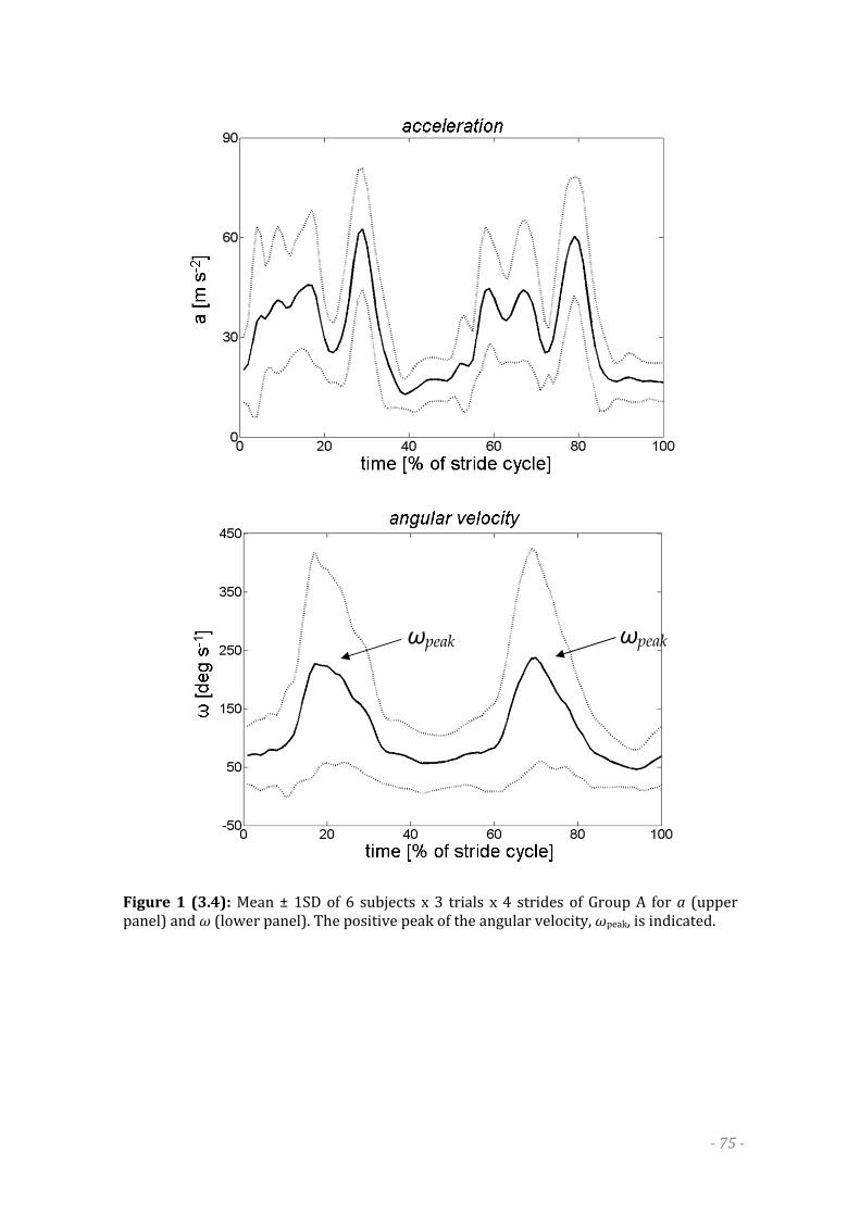
- 75 -

Figure 1 (3.4): Mean ± 1SD of 6 subjects x 3 trials x 4 strides of Group A for a (upper panel) and ω (lower panel). The positive peak of the angular velocity, ωpeak, is indicated.

ωpeak ωpeak

- 76 -

Figure 2 (3.4): Acceleration and angular velocity signals for three randomly selected subjects of group A, with reference to a randomly chosen stride cycle. Stride time is expressed in percentage of the total cycle duration. FS and FO events are indicated respectively with a circle and a square symbol.

- 77 -

Figure 3 (3.4): ω for three subjects of group A (left panel) and of group B (right panel), with reference to three randomly chosen stride cycles (blue, red and green curves). ωpeak was used to segment stride periods for both group A and B. Each period is expressed in percentage of the total cycle duration.

FS and FO instants were identified from positive and negative peaks on the

ω&& waveform (Fig. 4). These peaks were found to be consistently synchronized

with FS and FO across steps, trials, subjects and groups.

No repeatable and consistent features, adequate for automatic detection of

FS and FO related events, were identified on the two derivatives of a, neither in

group A nor in group B.

Repeated-measures ANOVA performed on the estimated parameters d~

stance

and d~

stride showed that no statistical differences across subjects (p > 0.05) and

trial (p > 0.05) was present in both groups A and B. Conversely, as expected,

statistical difference were found between groups (p < 0.05) for both d~

stance and

- 78 -

d~

stride. Tab. 2 reports the mean ± one standard deviation values of d~

stance and

d~

stride for both group A and group B.

Figure 4 (3.4): ω (grey dotted line), ω& (dashed line) and ω&& (solid line) with reference to a randomly chosen subject of group A. Grey sections represent three consecutive stance phases.

GROUP A GROUP B mean SD mean SD

d~

stance 0.125 ± 0.015 0.105 ± 0.010

d~

stride 0.495 ± 0.040 0.455 ± 0.015

Table 2 (3.4): Mean ± 1SD of d~

stance and d~

stride across of all the subjects, trials and steps is provided for both group A and group B.

Bland and Altman plots illustrating the results about the accuracy of the

stance duration estimates ( d~

stance) are shown in Fig. 5 for both group A (upper

panel) and group B (lower panel). The mean of the absolute bias between the

reference and the IMU estimates was 0.005 for both group A and B, as well as for

both d~

stance and d~

stride. The 95% of the limits of agreements was lower than 0.02 s

for both groups. Symmetry of the bias limits of agreement (LOA) interval was

observed, thus demonstrating that no systematic differences were present

- 79 -

between reference and IMU estimates. No linear trend between the amount of bias

and the measured values was found (average correlation = 0.02).

Figure 5 (3.4): Bland and Altman plots for group A and group B, corrected for the effect of repeated measurement error, representing comparisons between reference stance times and those estimated with IMU. Mean bias (solid line) and random error lines representing 95% limits of agreement (dashed lines) are included.

No differences were found across groups (p > 0.05), subjects (p > 0.05), and

trials (p > 0.05) for each parameter bias.

- 80 -

3.4.4 Discussion

The feasibility of using a trunk-mounted IMU for estimating the stance

duration during sprint running was assessed, and the accuracy of the IMU

estimates quantified against reference measurements. The results show that

neither the magnitude of the measured acceleration, nor its first and second

derivatives provide any consistent and well identifiable feature correlated with FS

and FO events. Conversely, the magnitude of the angular velocity vector, as well as

its wavelet-mediated second derivative, are characterised by repeatable and

consistent events correlated to stride and stance duration, respectively.

The identification on the acceleration time-series of features adequate for

automatic detection and related to the FS and FO events was thwarted mainly by

the low signal to noise ratio. The accelerometer signals, in fact, proved to be more

subjected to the movement of the soft tissue masses relative to the underlying

bones, with respect to the angular velocity measurements. Although each foot-

ground impact was visible on the time history of the acceleration magnitude,

neither FS nor FO events occurred at consistent maxima, minima, or even slope

across different subjects. This seems to be in contrast with previous studies using

trunk-mounted accelerometers during distance running. Wixted et al. (2010)

reported, on a qualitative level, that the vertical, medio-lateral and antero-

posterior acceleration curves of two professional middle-distance athletes have

significant features that can be used in analysis of athletes’ running style. Similarly,

Auvinet et al. (2002) qualitatively showed a substantial consistency among the

cranio-caudal, medio-lateral, and antero-posterior acceleration signals of seven

professional middle-distance runners. However, neither study provides validation

about the features consistency or about FS and FO event detection. In addition,

each component of the accelerometer is subjected to the variability entailed in the

sensor positioning. Using the magnitude of the acceleration vector means that the

user can fix the sensor unit in any orientation, thus requiring no anatomical

calibration or aligning protocols. This could be crucial in sports contexts, where

the acquisition procedures must not interfere with the training session schedule.

Finally, as distance running is characterised by a lower explosiveness with respect

to sprint running, the amount of IMU oscillations relative to the underlying

skeleton are lower, and the signal to noise ratio reasonably higher. This

- 81 -

consideration makes the above mentioned study conclusions hardly applicable to

sprint running.

The magnitude of the angular velocity signal presented a repeatable peak

that proved to be consistent across groups, subject, and trials. As reported in the

literature, this peak is associated to a trunk rotation about its longitudinal axis

(Schache, et al., 2002). Such rotation occurs during walking as well as during

running, and it is proved to be repeatable and to increase its amplitude with speed

(Saunders, et al., 2005). Our results confirm the presence of this rotation during

sprint running and prove that it is consistent among subjects with different

expertise. Although this event can be used to identify the stride duration, it does

not provide any information about the FS instant of time, thus about the stance

duration.

Such parameter was consistently identified only when using a wavelet-

mediated differentiation of ω that allowed for the identification on the ω&&

waveform of positive and negative peaks associated to the FS and FO events. From

a mechanical perspective, the local maxima associated to the FS is related to the

maximal variation of the angular acceleration of the trunk, while the local minima

associated to the FO is related to the trunk rotation about its longitudinal axis.

Both features proved to be repeatable and consistent among all subjects and trials.

The absolute bias between the IMU estimates and the reference

measurements was lower than 0.01 s for both d~

stride (< 2% stride duration) and

d~

stance (< 8% stance duration). These results are consistent with those obtained by

Purcell et al. (2006) as concerns the stance duration during sprint running using a

shank-mounted accelerometer.

It has to be noted that the mean stance durations for both group A and B

were higher than 0.1 s and that the mean difference of dstance between the two

groups of athletes involved in the present study was about 0.02 s, thus higher with

respect to such bias. An error lower than 0.01 s appears to be acceptable also when

considering the stance profile over time and during the whole race. Fig. 6 shows

such profile for both the stance and the flight phases as obtained from a high-speed

camera positioned behind the start line during one 80 m runs of an elite athlete of

group B. The stance duration decreases of about 0.07 s during the acceleration

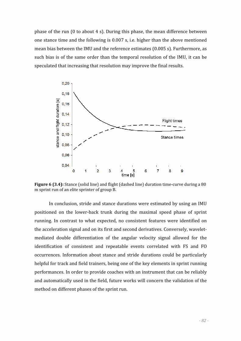
- 82 -

phase of the run (0 to about 4 s). During this phase, the mean difference between

one stance time and the following is 0.007 s, i.e. higher than the above mentioned

mean bias between the IMU and the reference estimates (0.005 s). Furthermore, as

such bias is of the same order than the temporal resolution of the IMU, it can be

speculated that increasing that resolution may improve the final results.

Figure 6 (3.4): Stance (solid line) and flight (dashed line) duration time-curve during a 80 m sprint run of an elite sprinter of group B.

In conclusion, stride and stance durations were estimated by using an IMU

positioned on the lower-back trunk during the maximal speed phase of sprint

running. In contrast to what expected, no consistent features were identified on

the acceleration signal and on its first and second derivatives. Conversely, wavelet-

mediated double differentiation of the angular velocity signal allowed for the

identification of consistent and repeatable events correlated with FS and FO

occurrences. Information about stance and stride durations could be particularly

helpful for track and field trainers, being one of the key elements in sprint running

performances. In order to provide coaches with an instrument that can be reliably

and automatically used in the field, future works will concern the validation of the

method on different phases of the sprint run.

- 83 -

3.5 LOW RESOLUTION APPROACH: DISCUSSION

The purpose of the Low Resolution Approach section was to develop

methods for the assessment of performance-related biomechanical variables in

sports applications. To this aim, the use of wearable inertial sensors for in-field

performance evaluation of sprint running was discussed.

Results confirmed the agreement between the estimated quantities

(instantaneous horizontal velocity, center of mass displacement, stride and stance

durations, trunk inclination and angular velocity), and the reference data provided

by stereophotogrammetry, force plates or high–speed cameras.

Two major sources of error proved to be crucial in the estimation of the

above mentioned parameters: the movement of soft tissue masses relative to the

underlying skeleton (soft tissue artefact) and the unstable bias characterising the

sensors signals. The latter, in particular, rapidly accumulates over time when

numerical integration of the measured signals is performed (for instance, to

estimate instantaneous velocity or displacement from the acceleration, or angular

displacement from the angular velocity). The explosiveness and high acceleration

generated during sprint running and, in general, during sports activities emphasise

the contribution of both sources of error.

The use of memory foam materials and elastic belts appears to be effective in

limiting the soft tissues movement, while reducing the integration interval and

exploring boundary conditions proved to cyclically correct the errors yielded by

the unstable bias of the signal.

During sprint running, the acceleration signal was found to be more

influenced by the soft tissue artefact with respect to the angular velocity signal, as

attested by the impossibility to identify in the former repeatable and consistent

features. This can be explained by considering that the soft tissue masses tend to

move mainly along cranio-caudal and medio-lateral direction. Skin-mounted

sensors measuring linear quantities seem, therefore, more sensitive to such

artefact with respect to sensor measuring angular quantities.

It is worthwhile to underline that each new proposed method needs to be

validated before being considered reliable and accurate. To this aim, the use of

reference technologies characterised by higher accuracy with respect to the

- 84 -

proposed method is necessary. As largely emphasised, traditional motion analysis

instrumentations are limited in terms of portability and acquisition volume.

Therefore, to perform in-field validations of methods involving inertial sensors, the

currently available and used technologies are essentially photocells, laser-gun, in-

shoe pressure sensors and high-speed cameras. Depending on the variable of

interest, however, the accuracy of these technologies could be lower with respect

to the accuracy of stereophotogrammetry or force plates, and sometimes could be

inadequate. As a result, a step-by-step approach including in-lab validation could

be, in some cases, mandatory. In particular, when the considered motor act could

hardly be repeatable in a laboratory environment, the choice of analysing an

equivalent motor paradigm could be a valid alternative. Such motor paradigm

would be characterised by the same peak-to-peak values and rate of variation of

acceleration than the motor act of interest (or angular velocity, or force depending

on the aim of the study), with the advantage to be suitable for in-lab analysis.

That being said, inertial measurement units proved to be a valid alternative

to traditional laboratory-based instrumentations when performing in-field

evaluation of sprint running. Guidelines about the unit fixation appear particularly

helpful and suitable for sports application. The development of algorithms that can

minimise the detrimental effects of the above mentioned sources of error, while

transforming this data into reliable parameters suitable for use by coaches and

athletes continues to be a challenging exercise.

- 85 -

CHAPTER 4

HIGH RESOLUTION APPROACH

- 86 -

• E. Bergamini, H. Pillet, J. Hausselle, P. Thoreux, S. Guerard, V. Camomilla, A. Cappozzo, W.

Skalli – “Tibio-femoral joint constraints for bone pose estimation during movement using

multi-body optimization”. Gait & Posture, 2011. In press.

• E. Bergamini, H. Pillet, J. Hausselle, P. Thoreux, V. Camomilla, A. Cappozzo, W. Skalli –

“Distance variation between origins and insertions of the knee ligaments during flexion-

extension”, 2nd National Bioengineering Conference, July 2010, Torino (Italy).

• H. Pillet, E. Bergamini, J. Hausselle, P. Thoreux, A. Cappozzo, W. Skalli – “Repeatability of a

method to evaluate knee ligaments lengths during flexion-extension”, 10th Annual Meeting

of the International Society for Computer Assisted Orthopaedic Surgery, June 2010, Paris

(France).

• P. Thoreux, H. Pillet, E. Bergamini, J. Hausselle, A. Cappozzo, W. Skalli – “Répétabilité d’une

méthode d’évaluation de la variation de longueur des ligaments du genou au cours d’un

mouvement de flexion-extension”, 85th Meeting of the Société Française de Chirurgie

Orthopédique et Traumatologique, November 2010, Paris (France).

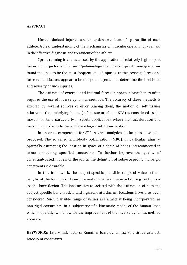
- 87 -

ABSTRACT

Musculoskeletal injuries are an undeniable facet of sports life of each

athlete. A clear understanding of the mechanisms of musculoskeletal injury can aid

in the effective diagnosis and treatment of the athlete.

Sprint running is characterised by the application of relatively high impact

forces and large force impulses. Epidemiological studies of sprint running injuries

found the knee to be the most frequent site of injuries. In this respect, forces and

force-related factors appear to be the prime agents that determine the likelihood

and severity of such injuries.

The estimate of external and internal forces in sports biomechanics often

requires the use of inverse dynamics methods. The accuracy of these methods is

affected by several sources of error. Among them, the motion of soft tissues

relative to the underlying bones (soft tissue artefact – STA) is considered as the

most important, particularly in sports applications where high acceleration and

forces involved may be cause of even larger soft tissue motion.

In order to compensate for STA, several analytical techniques have been

proposed. The so called multi-body optimization (MBO), in particular, aims at

optimally estimating the location in space of a chain of bones interconnected in

joints embedding specified constraints. To further improve the quality of

constraint-based models of the joints, the definition of subject-specific, non-rigid

constraints is desirable.

In this framework, the subject-specific plausible range of values of the

lengths of the four major knee ligaments have been assessed during continuous

loaded knee flexion. The inaccuracies associated with the estimation of both the

subject-specific bone-models and ligament attachment locations have also been

considered. Such plausible range of values are aimed at being incorporated, as

non-rigid constraints, in a subject-specific kinematic model of the human knee

which, hopefully, will allow for the improvement of the inverse dynamics method

accuracy.

KEYWORDS: Injury risk factors; Running; Joint dynamics; Soft tissue artefact;

Knee joint constraints.

- 88 -

4.1 INTRODUCTION

4.1.1 Sport biomechanics and injury prevention

This section was written on the basis of a book chapter by Zernicke, R.F., & Whiting,

W.C. (2000). Mechanisms of musculoskeletal injury in biomechanics in sport:

performance enhancement and injury prevention. In: Zatsiorsky, V.M. (Ed.), IOC

Medical Commission, International Federation of Sports. The authors’ work is

gratefully acknowledged.

Injury is an undeniable facet of athletic life. Individuals across the spectrum

of competitive levels, from recreational athletes to Olympic competitors, are

subject to the limitations and disappointments imposed by musculoskeletal injury.

Elite athletes, in particular, are highly susceptible to the physical, emotional, and

economic costs that injury exacts. Though these costs are inconsequential for

minor injuries, they can be overwhelming in cases of devastating injury that make

it impossible, either temporarily or permanently, for an athlete to train and

compete.

Lessening the chance of injury and facilitating the treatment and recovery of

injured athletes requires an interdisciplinary approach that includes consideration

of the anatomical, physiological, medical, kinesiological, psychological, and

mechanical aspects of athletes and their competitive environments. Unfortunately,

injury-related problems of athletes are not addressed optimally by each discipline

acting in isolation, especially for elite athletes whose performances are too often

considered more important than their health. An interdisciplinary team, including

medical professionals, physical therapists, athletic trainers, sport scientists,

psychologists, and coaches, is essential to bring a specific perspective to the

challenges of dealing with injuries to athletes. In addition to these individual

perspectives, musculoskeletal injury can be viewed from many different general

perspectives, including historical, epidemiological, economic, psychological and

biomechanical.

Of all scientific disciplines, physics and its sub-discipline, mechanics, are

undeniably most central to the study of injury, since most injuries have

mechanically related causes. The nature of an injury and its treatment rests on the

effective integration of biological and mechanical knowledge. Interdisciplinary

- 89 -

biomechanics (i.e. the application of mechanical principles to biological problems)

is ideally positioned to provide this integrated perspective. In the case of

musculoskeletal injury to athletes, the problems include those related to the

prevention, diagnosis, and treatment of injuries so as to minimize their incidence

and severity. The goal is to mitigate the negative effects of injury and allow athletes

at all levels to maximise their performance potential.

As above mentioned, a comprehensive analysis of a movement pattern or

skill requires not only the assessment of movement from a descriptive point of

view (kinematics), but also knowledge of the causes that produce the movement

(dynamics or kinetics). The word “cause” in mechanics, is always associated with

the concept of force, defined as the mechanical action applied to a body that tends

to produce acceleration.

Body movements are produced and controlled by forces acting both within

the body (e.g. muscle forces) and upon the body from external sources (e.g. gravity,

impact). These forces, in addition to modulating movement patterns, also act on

tissues in the body. Under most conditions, these forces are well tolerated by the

body’s tissues. Indeed, force is central to optimal growth and development of

tissues, especially those such as bone that provide structural support. But when

forces exceed a tissue’s ability to withstand the load, injury occurs. Forces and

force-related factors (e.g. energy), therefore, are the most fundamental element in

injuries and the prime agents that determine the likelihood and severity of a

specific injury (Zernicke & Whiting, 2000).

Forces pertinent to injury analysis include those that act in or upon the

human body, and include gravity, impact (e.g. a runner’s foot contact with the

ground), musculo-tendinous forces, ligamentous forces that stabilize joints, and

forces applied to bones. For all injury-related forces, different factors combine to

determine the nature and severity of the injury (Zernicke & Whiting, 2000): the

magnitude, application point, line of action and duration of the applied force, as

well as its frequency and rate of variability.

During athletic activities, body tissues are continuously subjected to forces

that vary in magnitude, location, direction, duration, frequency, variability and

rate. In most cases, the body tolerates these forces well, but when loads exceed the

normal physiological range, a not uncommon occurrence in elite athletes, tissues

- 90 -

can experience overload and sustain injury. Injuries resulting from a single or a

few overload episodes are called acute injuries. These injuries often happen with a

violent impact, such as when an object such as a ball contacts an athlete, or when

an athlete impact on the ground, like a runner at the foot-ground contact

followiong the flight phase, or a gymnast landing after a somersault. In general, as

the area of force application increases, thus decreasing the pressure, the likelihood

of injury decreases. When repeated loading leads to tissue damage, the injury is

called an overuse or chronic injury. Calcaneal (Achilles) tendonitis in a long-

distance runner provides one example of a chronic, overuse injury (Zernicke &

Whiting, 2000).

Sprint running injuries: epidemiology

Epidemiological studies of running injuries found the knee to be the most

frequent site of injuries (Clement, Taunton, Smart, & McNicol, 1981; Maughan &

Miller, 1983; Brunet, Cook, Brinker, & Dickinson, 1990) with chondromalacia

patella, pain on the undersurface of the patella, as one of the most frequent knee

injuries. Tab. 1 summarises the results from four epidemiological studies (James,

Bates, & Osternig, 1978; Clement, Taunton, Smart, & McNicol, 1981; Bennell &

Crossley, 1996; Ballas, Tytko, & Cookson, 1997) that attempted to identify the

source of lower-extremity injuries in running. It should be noted that the methods

used to collect injury statistics and the specific population sampled can have a

major effect on results, and such factors may account for some of the large

differences seen in the reported studies.

There is in general a paucity of scientific studies showing definitive


measures and injury. Nevertheless, kinetic factors that are thought to cause knee

injuries in runners include ground reaction and knee joint forces and moments

(Ferber, Kingma, Bruijn, & van Dieen, 2002).

Grimston et al. (1994) and Ferber et al. (2002) found greater ground

reaction forces in runners with stress fractures than in healthy runners. The

vertical impulse and propulsive forces, moreover, were found to be greater in

injured versus non-injured runners, but maximum vertical impact forces and

loading rates were lower in the injured groups (Messier & Pittala, 1988; Messier,

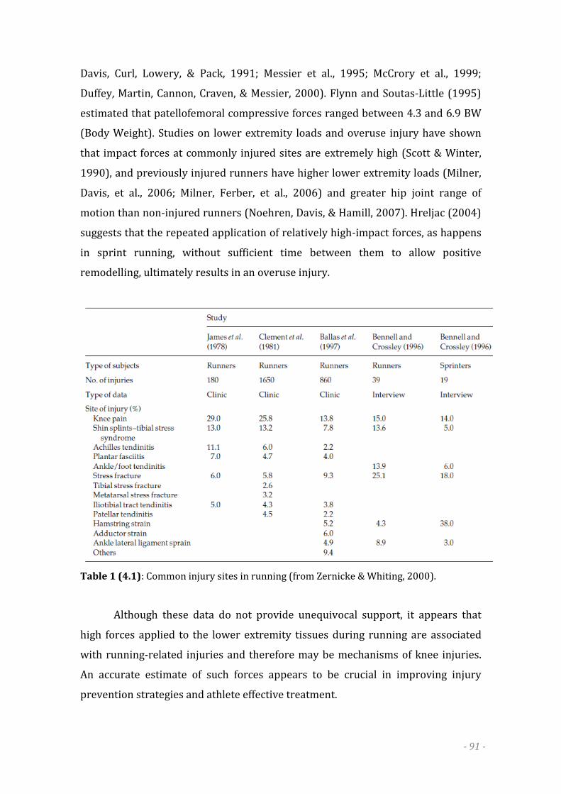
- 91 -

Davis, Curl, Lowery, & Pack, 1991; Messier et al., 1995; McCrory et al., 1999;

Duffey, Martin, Cannon, Craven, & Messier, 2000). Flynn and Soutas-Little (1995)

estimated that patellofemoral compressive forces ranged between 4.3 and 6.9 BW

(Body Weight). Studies on lower extremity loads and overuse injury have shown

that impact forces at commonly injured sites are extremely high (Scott & Winter,

1990), and previously injured runners have higher lower extremity loads (Milner,

Davis, et al., 2006; Milner, Ferber, et al., 2006) and greater hip joint range of

motion than non-injured runners (Noehren, Davis, & Hamill, 2007). Hreljac (2004)

suggests that the repeated application of relatively high-impact forces, as happens

in sprint running, without sufficient time between them to allow positive

remodelling, ultimately results in an overuse injury.

Table 1 (4.1): Common injury sites in running (from Zernicke & Whiting, 2000).

Although these data do not provide unequivocal support, it appears that

high forces applied to the lower extremity tissues during running are associated

with running-related injuries and therefore may be mechanisms of knee injuries.

An accurate estimate of such forces appears to be crucial in improving injury

prevention strategies and athlete effective treatment.

- 92 -

4.1.2 Joint dynamics estimation

Different techniques can be used to determine joint dynamics variables

(forces, moments and powers):

• Dynamometry: measurement of all or part of the scalar quantities that describe

a force system. Force platforms, based on strain-gauge or piezoelectric force

transducers are among the most used dynamometer in human movement

analysis.

• Inverse dynamics: estimation of the forces based on their observed effects on

the kinematics of the athlete’s body, i.e. on the time histories of the position and

orientation of the athlete’s body segments. Kinematic data are collected by

means of stereophotogrammetric motion capture systems. It has to be noted

that this approach allows for the determination of the resultant rather than

individual forces acting on the selected body part.

Although inverse dynamics is typically less accurate than direct

measurement, in some cases it is mandatory because the letter technique is not

applicable. When dealing with joint dynamics, for instance, it is often impossible to

directly measure internal forces such as those transmitted by muscles, tendons or

bones. This, indeed, would require the surgical implantation of a dynamometer in

the above mentioned intra or periarticular structures. In sports biomechanics,

moreover, it is even very difficult to measure external forces: dynamometers can

hardly be placed in fields, tracks, boards, gymnasium floors or equipment used for

sport competitions. On the other hand, as widely discussed in previous sections,

the majority of sports motor tasks can not be easily repeated in a motion analysis

laboratory, not mentioning athletes’ performances during competitions.

The accuracy of inverse dynamics is limited by several different sources of

error, including the simplifying assumptions used to define the mathematical

model of the human body. Among them, errors affecting the estimation of body

segment inertia parameters and those derived from the movement of soft tissues

(essentially muscles, fat tissue and skin) relative to the underlying bones are the

most critical in sports biomechanics.

While methods for accurately estimate inertial parameters have been

proposed and showed to be effective and relatively easy to be applied (de Leva,

1996), the errors associated to the soft tissue artefacts are much more difficult to

- 93 -

minimise and compensate for (Cappozzo, 1991; Leardini, Chiari, Della Croce, &

Cappozzo, 2005; de Leva & Cappozzo, 2006; Peters, Galna, Sangeux, Morris, &

Baker, 2010).

Different methods have been proposed to model the motion of the soft

tissue masses and of the bones separately, in order to obtain accurate estimates of

the resultant force applied on the body (Gruber, Ruder, Denoth, & Schneider, 1998;

Pain & Challis, 2006). De Leva and Cappozzo (2006) reported a peak error value of

-0.9 BW between measured and estimated vertical GRF of a volleyball player

performing four consecutive counter movement jumps with free arms. Their

results confirm that the difference between sports activities and daily motor tasks

considerably amplify the magnitude of STA and of its consequence on the estimate

of dynamic variables.

In order to compensate for STA, several analytical techniques have also

been proposed (Leardini, Chiari, Della Croce, & Cappozzo, 2005). All of them

exploit redundancy of measured information and embed a model of the artefact

(Soderkvist & Wedin, 1993; Cappello, Cappozzo, LaPalombara, Lucchetti, &

Leardini, 1997; Lucchetti, Cappozzo, Cappello, & Della Croce, 1998; Alexander &

Andriacchi, 2001). These techniques are either used to optimally estimate the pose

of one bony segment at a time (single-body optimization – SBO), and deal with all

of its six degrees of freedom, or aim at optimally estimating the location in space of

a chain of bones interconnected in joints embedding specified constraints (multi-

body optimization – MBO; in the literature often referred to as global

optimization). In the latter case, indeed, the available information about the

predictable behaviour of the main human joints, which imposes constraints to the

motion of the bones relative to each other, is aimed to be exploited. Recent studies

argue that more advanced joint models could actually reduce the errors associated

with skin marker-based measurement of joint (Andersen et al., 2009; Duprey, et

al., 2010). In this respect, the definition of proper joint constraints is crucial. To

this aim, the anatomy constitutes an ideal candidate to define subject-specific,

realistic and non-rigid constraints for models of the joint of interest.

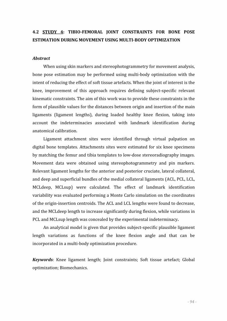
- 94 -

4.2 STUDY 4: TIBIO-FEMORAL JOINT CONSTRAINTS FOR BONE POSE

ESTIMATION DURING MOVEMENT USING MULTI-BODY OPTIMIZATION

Abstract

When using skin markers and stereophotogrammetry for movement analysis,

bone pose estimation may be performed using multi-body optimization with the

intent of reducing the effect of soft tissue artefacts. When the joint of interest is the

knee, improvement of this approach requires defining subject-specific relevant

kinematic constraints. The aim of this work was to provide these constraints in the

form of plausible values for the distances between origin and insertion of the main

ligaments (ligament lengths), during loaded healthy knee flexion, taking into

account the indeterminacies associated with landmark identification during

anatomical calibration.

Ligament attachment sites were identified through virtual palpation on

digital bone templates. Attachments sites were estimated for six knee specimens

by matching the femur and tibia templates to low-dose stereoradiography images.

Movement data were obtained using stereophotogrammetry and pin markers.

Relevant ligament lengths for the anterior and posterior cruciate, lateral collateral,

and deep and superficial bundles of the medial collateral ligaments (ACL, PCL, LCL,

MCLdeep, MCLsup) were calculated. The effect of landmark identification

variability was evaluated performing a Monte Carlo simulation on the coordinates

of the origin-insertion centroids. The ACL and LCL lengths were found to decrease,

and the MCLdeep length to increase significantly during flexion, while variations in

PCL and MCLsup length was concealed by the experimental indeterminacy.

An analytical model is given that provides subject-specific plausible ligament

length variations as functions of the knee flexion angle and that can be

incorporated in a multi-body optimization procedure.

Keywords: Knee ligament length; Joint constraints; Soft tissue artefact; Global

optimization; Biomechanics.

- 95 -

4.2.1 Introduction

Human movement analysis is largely based on the use of skin markers and

stereophotogrammetry. Since markers are not rigidly associated with the

underlying bone, bone pose reconstruction is affected by a soft tissue artefact

(STA). The magnitude of this artefact and its disruptive consequences on the

accuracy of the mechanical analysis of a motor act are well described in the

literature (Peters, et al., 2010).

In order to compensate for STA, several techniques have been proposed. All of

them exploit redundancy of measured information and embed a model of the

artefact (Soderkvist & Wedin, 1993; Chèze, Fregly, & Dimnet, 1995; Alexander &

Andriacchi, 2001). These techniques are either used to optimally estimate the pose

of one bony segment at a time (single-body optimization – SBO), and deal with all

of its six degrees of freedom, or aim at optimally estimating the location in space of

a chain of bones interconnected in joints embedding specified constraints (multi-

body optimization – MBO; often referred to as global optimization).

As opposed to the SBO, which deals only with the artefact deformation of

the cluster of markers, the MBO compensates also for its overall displacement

relative to the skeleton. In addition, the MBO may provide more realistic joint

kinematics by, for instance, preventing bones from appearing to macroscopically

pierce into each other. It should be noted however, that more realistic does not

necessarily mean more accurate and that, when using the MBO, the joint degrees of

freedom that are not embedded in the model are sacrificed.

Thus, MBO should not be expected to improve the estimate of joint

kinematics (Andersen, Benoit, Damsgaard, Ramsey, & Rasmussen, 2010), but to

provide an optimal reconstruction of the instantaneous location in space of the

entire chain of bones being analyzed. Therefore, a more accurate kinetic analysis is

made possible and the reconstruction of the movement of the soft tissue masses

relative to the underlying bone may be attempted. The latter movement may be fed

into a biodynamic model of the human body, the kinetic analysis of which would

incorporate the relevant inertial effects that are known to significantly affect the

forces involved in motor acts characterized by high accelerations (de Leva &

Cappozzo, 2006). These considerations justify investing resources aimed at

improving the MBO approach.

- 96 -

MBO has been performed mainly using joint constraints which prevent

translation, such as spherical, revolute or universal couplings (Lu & O'Connor,

1999; Andersen, et al., 2009). The knee has also been modelled using a parallel

mechanism incorporating articular surfaces, as sphere-on-plane contacts, and

isometric pseudo ligamentous structures, and allowing for both translations and

rotations (Duprey, et al., 2010).

To further improve the quality of these models, it is desirable to develop a

subject-specific kinematic model of the human knee which, during movement,

incorporates more realistic non-rigid constraints to the distances between the

origin and insertion landmarks (for simplicity referred to as lengths) of the four

major ligaments: anterior and posterior cruciate, and lateral and medial collateral

ligaments (ACL, PCL, LCL, MCL). These constraints can be represented by the

subject-specific plausible range of values of the ligament lengths for any given

flexion angle of the knee. It should be noted that these ranges of values, in order to

be incorporated in the above-mentioned knee model, must account for the

indeterminacies associated with the estimation of the subject-specific digital

models of the bones involved and of the location of the ligament origin and

insertion landmarks (anatomical calibration).

Several authors have focused on ligament kinematic behaviour with the aim

to support ligament injury treatment: ACL and PCL elongation was investigated ex-

vivo (Grood, Hefzy, & Lindenfield, 1989; Hollis, Takai, Adams, Horibe, & Woo,

1991) and in-vivo (Li, DeFrate, Sun, & Gill, 2004; Hosseini, Gill, & Li, 2009; Yoo et

al., 2010). Fewer studies have dealt with the MCL and LCL (Van de Velde et al.,

2007). However, most of these studies provide ligament lengths only for a few

knee flexion angles and do not display a general consensus about the amount and

direction of ligament length variation during flexion. In addition, the errors

associated with origin and insertion landmark identification have not been

accounted for. Thus, no general boundary conditions, as required in constraint-

based knee modelling, can be derived for the ligament lengths during continuous

flexion-extension.

The purpose of this study was to determine the above-mentioned plausible

values for the ligament lengths during loaded continuous healthy knee flexion. To

this aim, ex-vivo tibio-femoral joints were used to avoid soft tissue artefacts. Three-

- 97 -

dimensional digital models of tibias and femura were reconstructed and ligament

attachment areas identified on them together with the associated intra- and inter-

operator indeterminacies. The bone models were made to move in-silico using

experimental data obtained on the joint specimens. Ligament lengths were

thereafter estimated as a function of the joint flexion angle and submitted to

statistical analysis in order to provide a knee joint model that could be embedded

in the MBO procedure.


Six knee specimens, consisting of femur, patella, fibula and tibia and intact

joint passive structures, were harvested from subjects aged 75 to 96 years old and

fresh frozen. They exhibited no advanced osteoarthritis or ligament laxity and

presented no recurvatum.

The knee specimens were set in motion using a device described in Azmy et

al. (Azmy, Guérard, Bonnet, Gabrielli, & Skalli, 2010). The femur was fixed to the

experimental jig and the tibia caused to move by a servo-actuator that applied a

force to the quadriceps tendon that simulated a contraction of this muscle group. A

flexion resistive moment was applied to the knee through two cables fixed to the

distal end of the tibia and passing through two pulleys coaxial with the centre of

the femoral head and located laterally and medially to it. The force transmitted by

these cables to the tibia was equal to 30 N and maintained bone coaptation.

Clusters made of three retro-reflective markers, with a minimal separation

of 50 mm, were secured to the femur and to the tibia, each using two pins (Fig. 1a,

1b). The marker-cluster 3D positions and orientations were reconstructed during

movement using a stereophotogrammetric system (Polaris, Nothern Digital Inc.,

Canada) at a rate of 60 samples per second.

3D digital template models of femur and tibia were obtained from CT-scan

images. The perimeters of the areas of origin and insertion of the ACL, PCL, LCL, as

well as of the deep and superficial bundles of the MCL (MCLdeep, MCLsup), were

identified and traced on the bone templates using the mouse pointer. This

procedure was performed seven times by one operator and once by three different

operators for a total of ten virtual palpations. The professionals involved were

orthopaedic surgeons and underwent a specific and meticulous training.

- 98 -

Figure 1 (4.2): (a) 2D images acquired with the stereoradiographic system. (b) Reconstruction of the femur and tibia 3D digital models together with the photogrammetric markers. (c) Femur system of reference [18]: OF (origin): mid point of the segment joining the centers of the two condylar spheres, obtained by least squares approximation of the posterior portion of the medial and lateral epicondyles; YF: axis going from OF to the centre of the femoral head; ZF: projection onto the plane orthogonal to YF of the segment joining the centres of the two condylar spheres (dashed line); XF: cross product between YF and ZF. (d) Tibia system of reference [18]: OT (origin): centroid of the tibial plateaux; YT: axis going from the centroid of the tibial pilon surface to the intersection between the principal inertial axis of the tibial diaphysis (dashed line) and the tibial plateaux surface; ZT: projection onto the plane orthogonal to YT of the segment joining the most posterior points of the tibial plateaux (dashed line); XT: cross product between YT and ZT.

Two orthogonal digital radiographs of each knee specimen were

simultaneously obtained using a low dosage X-ray system (EOS®, EOS-imaging,

France) (Fig. 1a). The 3D bone-models were obtained through a reconstruction

algorithm based on three steps: 1. identification and labelling of anatomical

landmarks on the radiographic images in order to set a parametric simplified

subject-specific model; 2. pre-morphing of the bone template to get an initial

estimate of the bone; 3. iterative deformation of the latter estimate, based on

parametric models and statistical inferences, until the best estimate of the subject-

specific bone-model, carrying marks indicating the selected ligament attachment

areas, was obtained (Fig. 1b) (Chaibi, et al., 2011). The root mean square

discrepancy between a digital model of a femur or tibia, as obtained using this

- 99 -

procedure, and the relevant CT-scan model, was assessed in a previous study and

found to be on average less than 1 mm (Chaibi, et al., 2011). Each subject-specific

bone-model was reconstructed twice by three operators.

Each specimen was subjected to six flexion-extension cycles during which

marker trajectories were recorded.

Anatomical frames of femur and tibia (Fig. 1c, 1d) were defined as

suggested in Schlatterer et al. (2009).

Using the marker coordinates in the EOS® frame, the subject-specific bone-

models and the relevant anatomical axes were registered with respect to the

movement data given in the stereophotogrammetric (global) frame. The knee joint

kinematics was then estimated using the Cardan convention and the sequence ZT,

XT, YT.

For each of the six knees, each knee-model reconstruction, each flexion-

extension cycle, and each virtual palpation, the centroids of the attachment areas

of each ligament were determined. The mean values and standard deviations (SDs)

of these centroid coordinates, as represented in the global frame, were calculated.

It must be noted that virtual palpation did not display any significant difference

between inter and intra-operator variability.

The Euclidean distances between the mean origin and insertion centroids,

obtained averaging the ten virtual palpations, were then computed during the knee

movement (dc) (Fig. 2).

A similarity analysis of dc vs. flexion angle curves, as obtained from the six

flexion-extension cycles, was performed (r = 0.98±0.01; RMSE = 0.15±0.01 mm).

Results showed that no significant hysteresis occurred, thus, only mean curves

were considered for further analysis.

At this point, for each knee the data set was made of six curves, one for each

knee-model reconstruction.

In order to assess the impact of the inaccuracies associated with the

subject-specific bone-model reconstruction procedure on the estimation of

ligament length, a parametric statistical analysis was carried out by making

reference to the values of dc at full knee extension (de). To this purpose the

intraclass correlation coefficient (ICC) (McGraw & Wong, 1996) was calculated and

- 100 -

the Bland and Altman plots with correlation analysis of the bias between each

couple of operators inspected (Bland & Altman, 2010).

The propagation to the dc values of the errors associated with the variability

of the virtual palpation was assessed using a Monte Carlo simulation. Origin and

insertion points were randomly generated, using a normally distributed

mislocation from the mean centroid. The ligament length between each possible

pair of the generated origin and insertion points (100*100 pairs) was computed

during knee motion (dMC) (Fig.2).

Figure 2 (4.2): Digital model of a randomly chosen knee specimen: the ligament attachment areas and the tibio-femoral distances between the centroids (dc) (yellow lines) as well as between selected Monte Carlo pairs (dMC) (red lines) are depicted.

For the sake of generalization, ligament length variations (∆dMC) were then

calculated relative to de and expressed as percentage of the latter value for each

sampled knee flexion angle. The mean value and standard deviation of ∆dMC were

then calculated for each Monte Carlo pair over the six knees and the six digital

model reconstructions. To facilitate embedding this information in the knee

kinematic model to be used in the MBO process, the mean of the curves ∆dMC vs

- 101 -

flexion angle thus obtained, plus and minus one SD, were fitted with a polynomial

regression function of the fifth order.

4.2.3 Results

Both the intra- and inter-operator variability displayed a SD lower than 2

mm for all ligaments with regard to the ligament origin and insertion coordinates

on subject-specific knee models. Thus, this value was conservatively used as the SD

of the normal distribution used in the Monte Carlo simulation.

With respect to the effect of the indeterminacies associated with the

subject-specific bone-model reconstruction on the estimate of de, a high intra-

operator (ICC = 0.936; Confidence Interval (CI) [0.894;0.961]) and inter-operator

(ICC = 0.974; CI [0.960;0.983]) repeatability was found. Bland and Altman plots

and correlation analysis on the residuals confirmed these results. The mean bias

and the bias correlation computed between each pair of operators were low, with

both CIs spanning the zero value, thus demonstrating that no systematic

differences were present among the operators (bias = 0.11 mm; CI [-0.309;0.530];

corr = 0.13; CI [-0.116;0.373]). Given the resulting repeatability, multiple

reconstructions from different operators were considered as repeated measures.

The variability of de over the six observations and averaged over the six knees was

measured by a SD equal to 2.3 mm for ACL, 1.9 mm for PCL, 2.4 mm for MCLdeep,

2.1 mm for MCLsup, and 1.7 mm for LCL.

In Fig. 3, the distance dc is represented against the knee flexion angle with

reference to a randomly chosen knee. The ACL, LCL, and MCLdeep displayed

consistent trends in all knees, while the PCL and the MCLsup did not. In Fig. 3, the

selected knee internal-external rotation and the ab-adduction angles are also

depicted vs the flexion angle. The other knees displayed virtually identical curves.

The mean and SD curves of ∆dMC are shown in Fig. 4 for each ligament. The

coefficients of the regression functions used to fit the displayed curves are

reported in Tab. 1. The mean of the residual error norm between the fitting

function and the original curve was lower than 0.7±0.4%.

- 102 -

Figure 3 (4.2): For one randomly selected knee specimen, the ligament lengths are depicted as a function of the knee flexion angle: mean of three operators times two reconstructions ± 1SD. The kinematics of the same knee is also shown in the bottom right panel.

- 103 -

Figure 4 (4.2): Distance variation patterns (mean ± 1SD) vs the knee flexion angle as obtained through the Monte Carlo simulation for each ligament, ∆dMC. Each variation is expressed as a percentage of the distance at knee maximal extension.

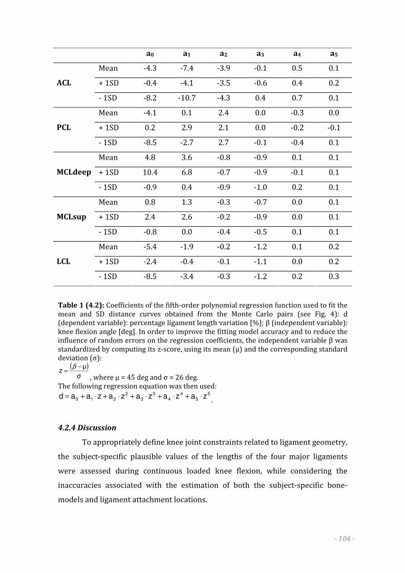
- 104 -

a0 a1 a2 a3 a4 a5

Mean -4.3 -7.4 -3.9 -0.1 0.5 0.1

+ 1SD -0.4 -4.1 -3.5 -0.6 0.4 0.2 ACL

- 1SD -8.2 -10.7 -4.3 0.4 0.7 0.1

Mean -4.1 0.1 2.4 0.0 -0.3 0.0

+ 1SD 0.2 2.9 2.1 0.0 -0.2 -0.1 PCL

- 1SD -8.5 -2.7 2.7 -0.1 -0.4 0.1

Mean 4.8 3.6 -0.8 -0.9 0.1 0.1

+ 1SD 10.4 6.8 -0.7 -0.9 -0.1 0.1 MCLdeep

- 1SD -0.9 0.4 -0.9 -1.0 0.2 0.1

Mean 0.8 1.3 -0.3 -0.7 0.0 0.1

+ 1SD 2.4 2.6 -0.2 -0.9 0.0 0.1 MCLsup

- 1SD -0.8 0.0 -0.4 -0.5 0.1 0.1

Mean -5.4 -1.9 -0.2 -1.2 0.1 0.2

+ 1SD -2.4 -0.4 -0.1 -1.1 0.0 0.2 LCL

- 1SD -8.5 -3.4 -0.3 -1.2 0.2 0.3

Table 1 (4.2): Coefficients of the fifth-order polynomial regression function used to fit the mean and SD distance curves obtained from the Monte Carlo pairs (see Fig. 4): d (dependent variable): percentage ligament length variation [%]; β (independent variable): knee flexion angle [deg]. In order to improve the fitting model accuracy and to reduce the influence of random errors on the regression coefficients, the independent variable β was standardized by computing its z-score, using its mean (μ) and the corresponding standard deviation (σ):

( )σ

µz

−=

β

, where µ = 45 deg and σ = 26 deg. The following regression equation was then used:

5

5

4

4

3

3

2

210zazazazazaad ⋅+⋅+⋅+⋅+⋅+= .

4.2.4 Discussion

To appropriately define knee joint constraints related to ligament geometry,

the subject-specific plausible values of the lengths of the four major ligaments

were assessed during continuous loaded knee flexion, while considering the

inaccuracies associated with the estimation of both the subject-specific bone-

models and ligament attachment locations.

- 105 -

The ACL and LCL were found to shorten during knee flexion reaching, on

average, 22% and 11% of their length at full extension, respectively. This is in

agreement with works reporting in-vivo behaviour of the ACL (Beynnon et al.,

2001; Li, et al., 2004; Hosseini, et al., 2009; Yoo, et al., 2010), ex-vivo behaviour of

the LCL (Harfe, Chuinard, Espinoza, Thomas, & Solomonow, 1998) and with a

simulation study involving both ligaments (Amiri, Cooke, Kim, & Wyss, 2007).

PCL length increased or decreased depending on the selected origin and

insertion location within the plausible area. This dependency has been already

evidenced ex-vivo (Grood, et al., 1989; Ahmad et al., 2003) and by using a

simulation approach (Amiri, et al., 2007). Conversely, in-vivo studies showed an

elongation of the central bundle of the PCL (DeFrate, Gill, & Li, 2004), as well as of

the antero-medial and postero-lateral ligament bundles (Li, et al., 2004). Since the

patterns of ligament length variation depend on the kinematics of the joint (Woo,

Debski, Withrow, & Janaushek, 1999; Amiri, et al., 2007), the lack of agreement

between in-vivo and ex-vivo, as well as simulation results might be attributed to

different amounts of tibial internal rotation during knee flexion, which the

referenced papers do not report. In-vivo knee kinematics was acquired during

quasi-static weight-bearing flexion (single-legged lunge using the free leg for

stability). Conversely, during ex-vivo studies, loaded knee flexion was obtained by

applying a force on the fixed femur (to the quadriceps tendon or to the patella,

when the patellar ligament was intact) and leaving the tibia free to move and

rotate, or similarly, fixing the tibia and allowing femur rotation.

Results on the deep and superficial bundle of the MCL must be interpreted

in the light of the following considerations. First, typical of the MCL is the critical

identification of its tibial origin, due to the lack of clear-cut bony prominences (Liu

et al., 2010). Second, most of the previous studies describe the length of the

ligament by a broken line wrapping around the most prominent edge of the tibial

plateau (Van de Velde, et al., 2007). Conversely, in the present work, consistently

with the proposed kinematic knee model, the length was computed as a Euclidean

distance. The MCLsup length increased or decreased depending on the selected

Monte Carlo pairs. This behaviour matches the results obtained in-vivo by Van de

Velde et al. (2007) who showed that, during knee flexion, the central, anterior, and

posterior bundles exhibited a nearly constant, increasing and decreasing length,

- 106 -

respectively. The average tendency of the MCLdeep length to increase during knee

flexion, accompanied by a maximal 10% shortening and 20% lengthening of

certain Monte Carlo pairs, is in partial in agreement with the results reported by

Van de Velde et al. (2007). These authors showed that the central bundle does not

change significantly its length, while the anterior bundle, on average, has a 10%

lengthening and the posterior bundle a 10% shortening.

The expertise and experience of the operators involved in this study is

supported by the low intra- and inter-operator variability in the identification of

the ligament attachment points, which was less than 2 mm. The Monte Carlo

simulation included a wide range of origin-insertion pairs and confirmed the

important effects of ligament attachment sites location on ligament length

variation. This has been shown previously, however, using fewer origin-insertion

points. Feeley et al. (2009) considered, for the MCLsup, five points on the femur

and four on the tibia, and others (Grood, et al., 1989; Schutzer, Christen, & Jakob,

1989) included less than ten combinations for the ACL and PCL.

Limitations of this study were that the ligaments involved belonged to

elderly individuals, with biased mechanical properties, and that an ex-vivo

experimental model was used. It may be assumed however, that in-vivo joint

kinematics of healthy subjects, under whatever external loading, is not different

from the kinematics obtained in this study to an extent that would cause a

significant change in ligament length behaviour. In both cases, in fact, stability or

coaptation of the joint should be guaranteed, although in a different manner, by a

synergic activity of both passive and active intra- and periarticular structures. This

hypothesis is supported by recent findings that, during a highly dynamic motion

such as the landing phase of a jump, showed that the ACL length decreases during

flexion by an amount similar to that obtained in the present study (Taylor, et al.,

2011).

In conclusion, the results of this study indicate that, in the framework of the

MBO approach, a kinematic model of the knee based on joint constraints should

consider the length of ACL, LCL and MCLdeep variable as a function of knee flexion.

Given the dependence of PCL and MCLsup length variation from the selected

attachment sites, these ligaments could be considered isometric. The efficacy of

this kinematic model, as opposed to those already implemented, must be evaluated

- 107 -

in terms of consequences on the estimate of joint kinetics, particularly when the

inertial effects of soft tissue masses are involved.

4.3 HIGH RESOLUTION APPROACH: DISCUSSION

The purpose of the High Resolution Approach section was to contribute

improving the accuracy of inverse dynamics methods for the estimation of joint

forces. The latter, in fact, are considered to be crucial in the assessment of injury-

related biomechanical variables in sports contexts. The evaluation of knee joint

forces, in particular, is very important during sprint running, being the knee the

most frequent site of injuries in this sports discipline.

In the framework of the multi-body optimization approach and to further

improve the quality of constraint-based kinematic models of the knee, subject-

specific, non-rigid constraints to the distances between the origin and insertion

landmarks of the four major knee ligaments were defined. The inaccuracies

associated with the estimation of the ligament attachment locations were also

considered.

Results indicated that, in a kinematic model of the knee based on joint

constraints, the length of the ACL, LCL and MCLdeep should be considered as

variable during knee flexion, while the length of the PCL and of the MCLsup proved

to be highly dependent from the selected attachment sites. These ligaments could

be, therefore, considered isometric during knee flexion.

The efficacy of this kinematic model, as opposed to those already

implemented, must be evaluated in terms of consequences on the estimate of joint

kinetics, particularly when the inertial effects of soft tissue masses are involved.

In addition, considering that the MBO technique aims at providing an

optimal estimation of the 3D position of the entire chain of bones in analysis, the

reconstruction of the movement of the soft tissue masses relative to the underlying

bone may also be attempted. It is worthwhile to underline, in fact, that such

movement is not an artefact in itself, but that it produces artefacts when it is used

to estimate the motion of the underlying bones. From a different perspective, it can

- 108 -

give unbiased information regarding the motion of some portions of soft tissues

and may be fed into a biodynamic model of the human body. The kinetic analysis of

this model would incorporate the relevant inertial effects that are known to

significantly affect the forces involved in motor acts characterized by high

accelerations, typical of sports applications. Preliminary tests showed that using a

large number of floating markers positioned on ad-hoc portions of the soft tissue

masses, thus exploiting redundancy of the measured information, appears to be

promising.

- 109 -

CHAPTER 5

CONCLUSIONS

- 110 -

Sports biomechanics describes the human movement from a performance


sports scientists is to support coaches and physicians with reliable and usable

information about athletes’ technique.

The lack of methods and protocols allowing for in-field athlete evaluation as

well as for accurate joint forces estimate represents, to date, the main limitation to

this purpose.

The results and the considerations carried out in the present thesis aim at

providing a contribution towards the development of the above mentioned

methods.

Results obtained from the Low Resolution Approach indicate that, due to

their portability and inexpensiveness, inertial measurement units proved to be a

valid alternative to traditional laboratory-based instrumentations, such as motion

analysis systems and force platforms. Their usability, moreover, contributes to

broaden the scope of application, allowing even coaches and runners to access

information regarding the influence of running mechanics on performance and

injuries.

Using acceleration and angular velocity measurements provided by the

inertial units, the following quantities were estimated: trunk inclination and

angular velocity, instantaneous horizontal velocity and displacement of a point

approximating the centre of mass, and stride and support phase durations.

The extraction of movement-related information from the measured

signals, however, is still demanding due to the movement of soft tissues relative to

the underlying skeleton and to the unstable bias characterising the sensors signals.

The latter proved to be relevant when numerical integration of the measured

signals is necessary. To mitigate these sources of error, particularly relevant when

dealing with sports motor acts, good-practice rules are recommended for the

benefit of signal processing. In particular, careful attention has to be paid to the

location and method of fixation of the sensor for limiting the motion of the soft

tissue masses. The use of memory foam materials and elastic belts appears to be

effective. To limit the errors yielded by the unstable bias of the signal, two

approaches can be used: reducing the integration interval, so that to limit the

- 111 -

amount of time in which errors accumulate, and exploring boundary conditions

which can be used to cyclically correct the drift errors, particularly, in non steady-

state movements.

In the framework of the multi-body optimization, High Resolution Approach

results indicate that, in a kinematic model of the knee based on joint constraints,

the length of the anterior cruciate, the lateral collateral and the deep bundle of the

medial collateral ligaments should be considered as variable during knee flexion.

The length of the posterior cruciate and of the superficial bundle of the medial

collateral ligaments was found to be highly dependent from the selected

attachment sites, and could be, therefore, considered isometric during knee

flexion.

These results represent a first contribution to the definition of methods

aiming at improving the accuracy of inverse dynamic estimates. The efficacy of a

kinematic knee model, as obtained by implementing constraints that are anatomy-

based, non-rigid and subject-specific must be evaluated, indeed, in terms of

consequences on the estimate of joint kinetics, particularly when the inertial

effects of soft tissue masses are involved.

The investment of resources aimed at improving the MBO approach,

however, is justified also by the following considerations: as the MBO techniques

aims at providing an optimal estimation of the 3D position of an entire chain of

bones (for instance pelvis, femur and tibia), the reconstruction of the movement of

the soft tissue masses relative to the underlying bone may be attempted. Such

movement may be then used to develop a biodynamic model of the human body,

which would incorporate the inertial effects known to significantly affect the forces

involved in motor acts characterized by high accelerations, typical of sports

applications. In this respect, using a large number of floating markers positioned

on ad-hoc areas of the soft tissue masses, thus exploiting redundancy of measured

information appears to be promising.

- 112 -

- 113 -

AKNOWLEDGEMENTS

The present thesis was developed in the framework of a co-tutoring agreement

between the Università degli Studi di Bologna and the Arts et Métiers ParisTech. The

financial support of the Università Italo-Francese (Call Vinci – Chapter II) is

gratefully acknowledged.

What I like the most of every “long trip”, is the opportunity to share it with other

people. It is with great pleasure and great pride that I thank all of you…for your scientific

and, especially, for your human contribution to my personal growth.

GRAZIE DI CUORE…

Al prof. Aurelio Cappozzo, per il suo grande carisma, per avermi mostrato cosa è il “rigore”, dal punto di vista scientifico ed umano, e per avermi insegnato

come forma e contenuto possano, e debbano, sempre coincidere.

A Valentina, per tutto ciò che abbiamo condiviso…con la speranza che questo viaggio abbia rappresentato, anche per lei, una proficua occasione di

crescita.

A Pietro (come avrei fatto senza di lui!), Mounir (per la sua inesauribile positività), Ilaria (la mia “roman dialect coach”), Marco D. (per la sua saggezza, informatica e non solo), Marco I. (per il suo humour romano), Luca (per la sua

sicula solarità), Marco F. (“er prinscipà”), Giuseppe (grande papà), Claudia (bignami di ottimi ristoranti romani), Paolo (“multiprod”), Elif e Alper (per la loro

sincera amicizia), Andrea (per i suoi preziosi consigli), Flaminia (per la sua spontaneità), i nuovi colleghi Eleni, John e Vincent...e naturalmente a Giorgio

(esempio di vita): è grazie a tutti voi che è sempre valsa la pena di affrontare i lunghi viaggi quotidiani.

A coach Filippo di Mulo, ai velocisti della Nazionale Italiana e agli atleti dello IUSM, per aver corso anche per noi.

MERCI BEAUCOUP…

A Mme Wafa Skalli, pour m’avoir accueillie dans son laboratoire à Paris, en contribuant à ma formation scientifique et culturelle.

A Hélène, pour m’avoir montré comment vie professionnelle et vie personnelle peuvent trouver un équilibre harmonieux et productif ; pour son aide,

- 114 -

son affection et sa proximité. Naturellement, merci à Guillaume et à la petite Lucie, pour toutes les fois où j’ai pu loger chez eux et, surtout, pour leur amitié…

A Pélagie, pour sa détermination, sa force et sa bonne humeur et parce que cela a été vraiment amusante de travailler ensemble ! Merci à ses parents, à

Mathilde et à Karim aussi, pour leur immense et inépuisable gentillesse et hospitalité.

A touts les collègues du LBM et, en particulier, à Xavier B., Elizabeth, Jérôme, Céline, Nicholas, Sandra, Xavier D., Aurélien, Amine, Marine, parce que si mes

séjours parisiens ont été autant agréables c’est aussi grâce à eux.

A Mme Patricia Thoreux, pour sa gentillesse et son aide dans la recherche scientifique et du logement à Paris. Et merci à Mme Véronique Digan, pour sa

disponibilité et gentillesse pendant mon séjour à Paris XIII.

A M. Lavaste, pour sa, toujours agréable, cordialité.

A toutes les personnes du CERAH de Paris, à Adrien Michel, à Mme Françoise Natta et à tous les athlètes qui ont participé aux expérimentations

parisiennes, pour leur collaboration et leur disponibilité.

E NATURALMENTE GRAZIE…

A Sara (la mia compagna di viaggio ideale…n’importe quel voyage), Chiara, Simone, Francesca e a tutti gli amici “del nord”, per non avermi mai fatto sentire la

loro mancanza, nonostante la distanza Bergamo-Roma.

A mamma Lucia, papà Giacomo, i miei fratelli Filippo, Paolo e Marco, ad Anna, la piccola Clara, Grazia e Franco, per l’esempio che da sempre rappresentano

e perché la loro vicinanza è stata, come sempre, determinante.

Ed infine ad Alberto. A lui, anche questa volta, spetta il mio “grazie” più

grande. Perché, più di tutti, ha condiviso con me ogni momento di questo viaggio. Per avermi sostenuto, consigliato, spronato, supportato e aspettato…anche

quando era difficile farlo. Per tutto questo…e per molto molto di più, GRAZIE.

- 115 -

- 116 -

- 117 -

REFERENCES

• Ahmad, C.S., Cohen, Z.A., Levine, W.N., Gardner, T.R., Ateshian, G.A., & Mow, V.C. (2003). Codominance of the individual posterior cruciate ligament bundles - An analysis of bundle lengths and orientation. American Journal of Sports Medicine, 31(2), 221-225.

• Ahmadi, A., Rowlands, D.D., & James, D.A. (2006). Investigating the translational and rotational motion of the swing using accelerometers for athlete skill assessment. IEEE Conference on Sensors, 5, 980-983.

• Alexander, E.J., & Andriacchi, T.P. (2001). Correcting for deformation in skin-based marker systems. Journal of Biomechanics, 34(3), 355-361.

• Aminian, K., Najafi, B., Büla, C., Leyvraz, P.F., & Robert, P. (2002). Spatio-temporal parameters of gait measured by an ambulatory system using miniature gyroscopes. Journal of Biomechanics, 35(5), 689-699.

• Amiri, S., Cooke, D., Kim, I.Y., & Wyss, U. (2007). Mechanics of the passive knee joint. Part 2: interaction between the ligaments and the articular surfaces in guiding the joint motion. Proceedings of the Institution of Mechanical Engineers Part H-Journal of Engineering in Medicine, 221(H8), 821-832.

• Andersen, M.S., Benoit, D.L., Damsgaard, M., Ramsey, D.K., & Rasmussen, J. (2010). Do kinematic models reduce the effects of soft tissue artefacts in skin marker-based motion analysis? An in vivo study of knee kinematics. Journal of Biomechanics, 43(2), 268-273.

• Andersen, M.S., Damsgaard, M., & Rasmussen, J. (2009). Kinematic analysis of over-determinate biomechanical systems. Computer Methods in Biomechanics and Biomedical Engineering, 12(4), 371-384.

• Atkinson, G., & Nevill, A.M. (1998). Statistical methods for assessing measurement error (reliability) in variables relevant to sports medicine. Sports Med, 26(4), 217-238.

• Atwater, A.E. (1982). Kinematic analysis of spinting. Track and Field Q Rev, 82(2), 12-16.

• Auvinet, B., Gloria, E., Renault, G., & Barrey, E. (2002). Runner’s stride analysis: comparison of kinematic and kinetic analyses under field conditions. Science & Sports, 17, 92-94.

• Azmy, C., Guérard, S., Bonnet, X., Gabrielli, F., & Skalli, W. (2010). EOS® orthopaedic imaging system to study patellofemoral kinematics: Assessment of uncertainty. Orthopaedics & Traumatology: Surgery & Research, 96(1), 28-36.

• Baca, A. (2006). Innovative diagnostic methods in elite sport. International Journal of Performance Analysis in Sport, 6, 148-156.

• Bachmann, E.R. (1999). Orientation tracking for humans and robots using inertial sensors. Proceedings of the 3rd International Symposium on Computational Intelligence in Robotics & Automation, Monterey, CA (USA).

- 118 -

• Ballas, M.T., Tytko, J., & Cookson, D. (1997). Common overuse running injuries: diagnosis and management. Am Fam Physician, 55(7), 2473-2484.

• Bartlett, R. (2006). Artificial intelligence in sports biomechanics: new dawn or false hope? Journal of Sports Science and Medicine, 5, 474-479.

• Baumann, W. (1976). Kinematic and dynamic characteristics of the sprint start. In Komi P.V., Biomechanics, University Park Press, Baltimore.

• Bennell, K.L., & Crossley, K. (1996). Musculoskeletal injuries in track and field: incidence, distribution and risk factors. Aust J Sci Med Sport, 28(3), 69-75.

• Beynnon, B.D., Uh, B.S., Johnson, R.J., Fleming, B.C., Renstrom, P.A., & Nichols, C.E. (2001). The elongation behavior of the anterior cruciate ligament graft in vivo - A long-term follow-up study. American Journal of Sports Medicine, 29(2), 161-166.

• Bland, J.M., & Altman, D.G. (2007). Agreement between methods of measurement with multiple observations per individual. J Biopharm Stat, 17(4), 571-582.

• Bland, J.M., & Altman, D.G. (2010). Statistical methods for assessing agreement between two methods of clinical measurement. International Journal of Nursing Studies, 47(8), 931-936.

• Bouten, C.V., Koekkoek, K.T., Verduin, M., Kodde, R., & Janssen, J.D. (1997). A triaxial accelerometer and portable data processing unit for the assessment of daily physical activity. IEEE Trans Biomed Eng, 44(3), 136-147.

• Brughelli, M., & Cronin, J. (2008). A review of research on the mechanical stiffness in running and jumping : methodology and implications. Scandinavian Journal of Medicine & Science in Sports, 417-426.

• Brunet, M.E., Cook, S.D., Brinker, M.R., & Dickinson, J.A. (1990). A survey of running injuries in 1505 competitive and recreational runners. J Sports Med Phys Fitness, 30(3), 307-315.

• Butler, R.J., Crowell, H.P., & Davis, I.M. (2003). Lower extremity stiffness: implications for performance and injury. Clin Biomech (Bristol, Avon), 18(6), 511-517.

• Butler, R.J., Davis, I.S., & Hamill, J. (2006). Interaction of arch type and footwear on running mechanics. Am J Sports Med, 34(12), 1998-2005.

• Burr, D.B., Martin, R.B., Schaffler, M.B., & Radin, E.L. (1985). Bone remodeling in response to in vivo fatigue microdamage. Journal of Biomechanics, 18, 189-200.

• Camomilla V., Lupi, C., & Picerno, P. (2008). An in field forehand stroke evaluation using wearable inertial sensors. Coaching and Sport Science Journal, 3(2), 23-24.

• Cappellini, G., Ivanenko, Y.P., Poppele, R.E., & Lacquaniti, F. (2006). Motor patterns in human walking and running. J Neurophysiol, 95(6), 3426-3437.

• Cappello, A., Cappozzo, A., LaPalombara, P.F., Lucchetti, L., & Leardini, A. (1997). Multiple anatomical landmark calibration for optimal bone pose estimation. Human Movement Science, 16(2-3), 259-274.

- 119 -

• Cappozzo, A. (1991). Three-dimensional analysis of human walking - Experimental methods and associated artefacts. Human Movement Science, 10(5), 589-602.

• Cappozzo, A., De Vito, G., Gazzani, F., & Massacesi, R. (1989). Analisi biomeccanica della partenza dai blocchi. Atleticastudi, 347-375.

• Cappozzo, A., Della Croce, U., Leardini, A., & Chiari, L. (2005). Human movement analysis using stereophotogrammetry. Part 1: theoretical background. Gait & posture, 21(2), 186-196.

• Carling, C., & Williams, R. (2005). Handbook of soccer match analysis. A systematic approach. Routledge, Abingdom, UK.

• Carling, C., Reilly, T., & Williams, A.M. (2009). Performance Assessment for Field Sports: Physiological, Psychological and Match Notational Assessment in Practice. Routledge, Abingdom, UK

• Catalfamo, P., Moser, D., Ghoussayni, S., & Ewins, D. (2008). Detection of gait events using an F-Scan in-shoe pressure measurement system. Gait & Posture, 28(3), 420-426.

• Cavagna, G.A., Komarek, L., & Mazzoleni, S. (1971). The mechanics of sprint running. The Journal of Physiology Online, 217, 709-721.

• Cavanagh P.R. (1990). Biomechanics of distance running. Human Kinetics, Champaign, IL.

• Chaibi, Y., Cresson, T., Aubert, B., Hausselle, J., Neyret, P., Hauger, O., et al. (2011). Fast 3D reconstruction of the lower limb using a parametric model and statistical inferences and clinical measurements calculation from biplanar X-rays. Computer methods in biomechanics and biomedical engineering, in press.

• Channells, J., Purcell, B., Barrett, R., & James, D. (2005). Determination of rotational kinematics of the lower leg during sprint running using accelerometers. Proceedings of SPIE, 6036.

• Chèze, L., Fregly, B.J., & Dimnet, J. (1995). A solidification procedure to facilitate kinematic analyses based on video system data. Journal of Biomechanics, 28(7): 879-884.

• Ciacci, S., Di Michele, R., & Merni, F. (2010). Kinematic analysis of the braking and propulsion phases during the support time in sprint running. Gait & Posture, 31(2), 209-212.

• Clement, D.B., Taunton, J.E., Smart, G.W., & McNicol, K.L. (1981). A survey of overuse running injuries. Phys Sports Med, 9, 47-58.

• Clinghan, R., Arnold, G.P., Drew, T.S., Cochrane, L.A., & Abboud, R.J. (2008). Do you get value for money when you buy an expensive pair of running shoes? Br J Sports Med, 42(3), 189-193.

• Čoh, M., Jošt, B., Škof, B., Tomažin, K., & Dolenec, A. (1998). Kinematic and kinetic parameters of the sprint start and start acceleration model of top sprinters. Gymnica, 28, 33-42.

- 120 -

• Čoh, M., Tomažin, K., & Štuhec, S. (2006). The biomechanical model of the sprint start and block acceleration. Physical Education and Sport, 4, 103-114.

• Collier, C. (2002). Foundational Concepts of Sprinting: Spatial and Movement Perspectives. Track Coach, 5071-5077.

• Cousins, S., & Dyson, R. (2004). Forces at the front and rear blocks during the sprint start. Proceedings for the ISBS Conference, Ottawa, Canada, 198-201.

• Cronin, J., & Sleivert, G. (2005). Challenges in understanding the influence of maximal power training on improving athletic performance. Sports Med, 35(3), 213-234.

• de Leva, P. (1996). Adjustments to Zatsiorsky-Seluyanov's segment inertia parameters. Journal of Biomechanics 29(9), 1223-1230.

• de Leva, P., & Cappozzo, A. (2006). Estimating forces in sports biomechanics. In A. Rainoldi, M. A. Minetto & R. Merletti (Eds.), Turin (IT), 71-88.

• DeFrate, L.E., Gill, T.J., & Li, G. (2004). In vivo function of the posterior cruciate ligament during weightbearing knee flexion. American Journal of Sports Medicine, 32(8), 1923-1928.

• Derrick, T.R., Dereu, D., & McLean, S.P. (2002). Impacts and kinematic adjustments during an exhaustive run. Med Sci Sports Exerc, 34(6), 998-1002.

• Dierick, F., Penta, M., Renaut, D., & Detrembleur, C. (2004). A force measuring treadmill in clinical gait analysis. Gait and Posture, 20(3), 299-303.

• Dixon, S.J. (2008). Use of pressure insoles to compare in-shoe loading for modern running shoes. Ergonomics, 51(10), 1503-1514.

• Donati, M., Camomilla, V., Vannozzi, G., & Cappozzo, A. (2008). Anatomical frame identification and reconstruction for repeatable lower limb joint kinematics estimates. Journal of Biomechanics, 41(10), 2219-2226.

• Duffey, M.J., Martin, D.F., Cannon, D.W., Craven, T., & Messier, S.P. (2000). Etiologic factors associated with anterior knee pain in distance runners. Med Sci Sports Exerc, 32(11), 1825-1832.

• Dugan, S.A., & Bhat, K.P. (2005). Biomechanics and analysis of running gait. Phys Med Rehabil Clin N Am, 16(3), 603-621.

• Duprey, S., Cheze, L., & Dumas, R. (2010). Influence of joint constraints on lower limb kinematics estimation from skin markers using global optimization. Journal of Biomechanics, 43(14), 2858-2862.

• Faber, G.S., Kingma, I., Bruijn, S.M., & van Dieen, J.H. (2009). Optimal inertial sensor location for ambulatory measurement of trunk inclination. Journal of Biomechanics, 42(14), 2406-2409.

• Favre, J., Jolles, B.M., Siegrist, O., & Aminian, K. (2006). Quaternion-based fusion of gyroscopes and accelerometers to improve 3D angle measurement. Electronics Letters, 42(11), 612-614.

• Feeley, B.T., Muller, M.S., Allen, A.A., Granchi, C.C., & Pearle, A.D. (2009). Isometry of medial collateral ligament reconstruction. Knee Surgery, Sports Traumatology, Arthroscopy, 17(9): 1078-1082.

- 121 -

• Ferber, R.I., McClay-Davis, I., Hamill, J., Pollard, C.D., & McKeown, K.A. (2002). Kinetic variables in subjects with previous lower extremity stress fractures. Med Sci Sports Exerc, 34(S5).

• Flynn, T.W., & Soutas-Little, R.W. (1995). Patellofemoral joint compressive forces in forward and backward running. Journal of Orthopaedic & Sports Physical Therapy, 21(5), 277-282.

• Forner-Cordero, A., Mateu-Arce, M., Forner-Cordero, I., Alcántara, E., Moreno, J. C., & Pons, J. L. (2008). Study of the motion artefacts of skin-mounted inertial sensors under different attachment conditions. Physiological measurement, 29(4), N21-31.

• Fortier, S., Basset, F.A., Mbourou, G.A., Faverial, J., & Teasdale, N. (2005). Starting block performance in sprinters: A statistical method for identifying discriminative parameters of the performance and an analysis of the effect of providing feedback over a 6-week period. Journal of Sports Science and Medicine, 4(2), 134-143.

• Fyfe, K.R., & Gildenhuys, A.H. (2004). Foot path measurement using accelerometry. Proceedings of the ASB, 294.

• Goldsmith, W. (2000). Bridging the gap? Now there is a gap in the bridge! A.S.C.A. Newsletter, 3, 2-4.

• Goodvin, C., Park, E. J., Huang, K., & Sakaki, K. (2006). Development of a real-time three-dimensional spinal motion measurement system for clinical practice. Medical & Biological Engineering & Computing, 44(12), 1061-1075.

• Grimston, S.K., Nigg, B.M., Fisher, V., & Ajemian, S.V. (1994). External loads throughout a 45 minute run in stress fracture and non-stress fracture runners. Journal of Biomechanics, 27, 668.

• Grood, E.S., Hefzy, M.S., & Lindenfield, T.N. (1989). Factors affecting the region of most isometric femoral attachments: Part I: The posterior cruciate ligament. The American Journal of Sports Medicine, 17(2), 197-207.

• Gruber, K., Ruder, H., Denoth, J., & Schneider, K. (1998). A comparative study of impact dynamics: wobbling mass model versus rigid body models. Journal of Biomechanics, 31(5), 439-444.

• Hanlon, M., & Anderson, R. (2009). Real-time gait event detection using wearable sensors. Gait & posture, 30(4), 523-527.

• Harfe, D.T., Chuinard, C.R., Espinoza, L.M., Thomas, K.A., & Solomonow, M. (1998). Elongation patterns of the collateral ligaments of the human knee. Clinical Biomechanics, 13(3), 163-175.

• Harland, M.J., & Steele, J.R. (1997). Biomechanics of the sprint start. Sports Medicine, 23(1), 11-20.

• Harris, G.F., & Wertsch, J.J. (1994). Procedures for gait analysis. Arch. Phys. Med. Rehabil., 75, 216-225.

• Hay, J.G. (1993). The Biomechanics of Sports Techniques. 4th ed. London, Benjamin-Cummings Pub Co.

- 122 -

• Henry, F.M. (1954). Time-velocity equations and oxygen requirements of “all-out” and “steadypace” running. Res Q Exerc Sport, 25, 164-177.

• Hewett, T.E., Stroupe, A.L., Nance, T.A., & Noyes, F.R. (1996). Polymetric training in female athletes: decreased impact forces and decreased hamstring torques. Am. J. Sports Med., 24, 765-773.

• Higginson, B.K. (2009). Methods of running gait analysis. Curr Sports Med Rep, 8(3), 136-141.

• Hill, A.V. (1927). Muscular movement in man. McGraw-Hill Book Co., New York.

• Hinrichs, R.N., Cavanagh, P.R., & Williams, K.R. (1987). Upper extremity function in running: centre of mass and propulsion considerations. International Journal of Sports Biomechanics, 3, 222-241.

• Hobara, H., Inoue, K., Gomi, K., Sakamoto, M., Muraoka, T., Iso, S., et al. (2009). Continuous change in spring-mass characteristics during a 400 m sprint. J Sci Med Sport, 13(2), 256-261.

• Hollis, J.M., Takai, S., Adams, D.J., Horibe, S., & Woo, S.L.Y. (1991). The effects of knee motion and external loading on the length of the anterior cruciate ligament (ACL) - A kinematic study. Journal of Biomechanical Engineering, 113(2), 208-214.

• Hosseini, A., Gill, T.J., & Li, G.A. (2009). In vivo anterior cruciate ligament elongation in response to axial tibial loads. Journal of Orthopaedic Science, 14(3), 298-306.

• Hsiao, H., Guan, J., & Weatherly, M. (2002). Accuracy and precision of two in-shoe pressure measurement systems. Ergonomics, 45(8), 537-555.

• Hsich, Y. (1997). Knee kinematics and ligament lengths during physiologic levels of isometric quadriceps loads. The Knee, 4(3), 145-154.

• Hunter, J.P., Marshall, R.N., & McNair, P. (2004a). Reliability of biomechanical variables of sprint running. Medicine & Science in Sports & Exercise, 36(5), 850-850.

• Hunter, J.P., Marshall, R.N., & McNair, P.J. (2004b). Interaction of step length and step rate during sprint running. Med Sci Sports Exerc, 36(2), 261-271.

• Hunter, J.P., Marshall, R.N., & McNair, P.J. (2005). Relationships between ground reaction force impulse and kinematics of sprint-running acceleration. J Appl Biomech, 21(1), 31-43.

• Innocenti, B., Facchielli, D., Torti, S., & Verza, A. (2006). Analysis of biomechanical quantities during a squat jump: evaluation of a performance index. J Strength Cond Res, 20(3), 709-715.

• Ito, A., Ishikawa, M., Isolehto, J., & Komi, P.V. (2006). Changes in the step width, step length, and step frequency of the world’s top sprinters during a 100 m race. New Studies in Athletics, 21(3), 35-39.

• James, S.L., Bates, B.T., & Osternig, L.R. (1978). Injuries to runners. Am J Sports Med, 6(2), 40-50.

- 123 -

• James, D.A., Davey, N. & Rice, T., 2004. An accelerometer based sensor platform for insitu elite athlete performance analysis. IEEE Conference on Sensors, 3, 1373-1376.

• Jasiewicz, J.M., Allum, J.H., Middleton, J.W., Barriskill, A., Condie, P., Purcell, B., et al. (2006). Gait event detection using linear accelerometers or angular velocity transducers in able-bodied and spinal-cord injured individuals. Gait & Posture, 24(4), 502-509.

• Jianwen, L., Jing, B., & Jinhua, S. (2006). Application of the wavelet transforms on axial strain calculation in ultrasound elastography. Progress in Natural Science, 16(9), 942-947.

• Jidovtseff, B., Croisier, J.L., Lhermerout, C., Serre, L., Sac, D. and Crielaard, J.M. (2006). The concept of iso-inertial assessment: Reproducibility analysis and descriptive data. Isokinetics and Exercise Science, 14(1), 53-62.

• Jones, R., Bezodis, I., & Thompson, A. (2009). Coaching Sprinting: Expert Coaches' Perception of Race Phases and Technical Constructs. International Journal of Sports Science & Coaching, 4(3), 385-396.

• Jurman, D., Jankovec, M., Kamnik, R., & Topic, M. (2007). Calibration and data fusion solution for the miniature attitude and heading reference system. Sensors and Actuators a-Physical, 138(2), 411-420.

• Kalman, R.E. (1960). A new approach to linear filtering and prediction problems. Journal of basic Engineering, 82(1), 35-45.

• Karamanidis, K., Arampatzis, A., & Brüggemann, G.P. (2004). Reproducibility of electromyography and ground reaction force during various running techniques. Gait & Posture, 19(2), 115-123.

• Kavanagh, J.J., & Menz, H.B. (2008). Accelerometry: a technique for quantifying movement patterns during walking. Gait & Posture, 28(1), 1-15.

• Knudson, D. (2007). Qualitative biomechanical principles for application in coaching. Sports Biomech, 6(1), 109-118.

• Kraan, G.A., van Veen, J., Snijders, C.J., & Storm, J. (2001). Starting from standing; why step backwards? Journal of Biomechanics, 34(2), 211-215.

• Kugler, F., & Janshen, L. (2010). Body position determines propulsive forces in accelerated running. Journal of Biomechanics, 43(2), 343-348.

• Lafortune, M.A. (1991). Three-dimensional acceleration of the tibia during walking and running. Journal of Biomechanics, 24(10), 877-886.

• Lafortune, M.A., Henning, E., & Valiant, G.A. (1995). Tibial shock measured with bone and skin mounted transducers. Journal of Biomechanics, 28(8), 989-993.

• Latash, M.L., & Zatsiorsky, V.M. (1993). Joint stiffness: myth or reality?. Hum. Movement Sci. 12, 653–692.

• Le Bris, R., Billat, V., Auvinet, B., Chaleil, D., Hamard, L., & Barrey, E. (2006). Effect of fatigue on stride pattern continuously measured by an accelerometric gait recorder in middle distance runners. J Sports Med Phys Fitness, 46(2), 227-231.

- 124 -

• Leardini, A., Chiari, L., Della Croce, U., & Cappozzo, A. (2005). Human movement analysis using stereophotogrammetry - Part 3. Soft tissue artifact assessment and compensation. Gait & Posture, 21(2), 212-225.

• Lee, J.B., Mellifont, R.B., & Burkett, B.J. (2010). The use of a single inertial sensor to identify stride, step, and stance durations of running gait. Journal of Science and Medicine in Sport, 13(2), 270-273.

• Lee, J.B., Sutter, K.J., Askew, C.D., & Burkett, B.J. (2010). Identifying symmetry in running gait using a single inertial sensor. Journal of Science and Medicine in Sport, 13(5), 559-563.

• Lee, R. (2003). A real-time gyroscopic system for three-dimensional measurement of lumbar spine motion. Medical Engineering & Physics, 25(10), 817-824.

• Li, G., DeFrate, L.E., Sun, H., & Gill, T.J. (2004). In vivo elongation of the anterior cruciate ligament and posterior cruciate ligament during knee flexion. American Journal of Sports Medicine, 32(6), 1415-1420.

• Liu, F., Yue, B., Gadikota, H.R., Kozanek, M., Liu, W., Gill, T.J., et al. (2010). Morphology of the medial collateral ligament of the knee. J Orthop Surg Res, 5, 69.

• Liu, W., & Nigg, B.M. (2000). A mechanical model to determine the influence of masses and mass distribution on the impact force during running. Journal of Biomechanics, 33(2), 219-224.

• Lu, T.W., & O'Connor, J.J. (1999). Bone position estimation from skin marker co-ordinates using global optimisation with joint constraints. Journal of Biomechanics, 32(2), 129-134.

• Lucchetti, L., Cappozzo, A., Cappello, A., & Della Croce, U. (1998). Skin movement artefact assessment and compensation in the estimation of knee-joint kinematics. Journal of Biomechanics, 31(11), 977-984.

• Luinge, H.J., Veltink, P.H., & Baten, C.T. (1999). Estimating orientation with gyroscopes and accelerometers. Technology and Health Care, 7(6), 455-459.

• Luthanen, P., & Komi, P.V. (1978). Mechanical factors influencing running speed. In Asmussen, E., Jorgensen, K. (Eds). Biomechanics VI-B, Baltimore University Park Press, 23-29.

• Mann, R., Kotmel, J., & Herman, J. (2008). Kinematic trends in elite sprinters. Proccedings for the ISBS Conference, Seoul (Korea).

• Maughan, R.J., & Miller, J.D. (1983). Incidence of training-related injuries among marathon runners. Br J Sports Med, 17(3), 162-165.

• Mayagoitia, R.E., Nene, A.V., & Veltink, P.H. (2002). Accelerometer and rate gyroscope measurement of kinematics: an inexpensive alternative to optical motion analysis systems. Journal of Biomechanics, 35(4), 537-542.

• Mazzà, C., Iosa, M., Picerno, P., & Cappozzo, A. (2009). Gender differences in the control of the upper body accelerations during level walking. Gait & posture, 29(2), 300-303.

- 125 -

• McCrory, J.L., Martin, D.F., Lowery, R.B., Cannon, D.W., Curl, W.W., Read, H.M., et al. (1999). Etiologic factors associated with Achilles tendinitis in runners. Med Sci Sports Exerc, 31(10), 1374-1381.

• McGraw, K.O., & Wong, S.P. (1996). Forming inferences about some intraclass correlation coefficients. Psychological Methods, 1(1), 30-46.

• Mehrikadze, V., & Tabatschnik B. (1982). An Analysis of sprinting. Legkaja Atletika, 3, 8-10.

• Mercer, J.A., Bates, B.T., Dufek, J.S., & Hreljac, A. (2003). Characteristics of shock attenuation during fatigued running. J Sports Sci, 21(11), 911-919.

• Mero, A., & Komi, P.V. (1987). Electromyographic activity in sprinting at speeds ranging from sub-maximal to supra-maximal. Med Sci Sports Exerc, 19(3), 266-274.

• Mero, A., & Komi, P.V. (1990). Reaction time and electromyographic activity during a sprint start. Eur J Appl Physiol Occup Physiol, 61(1-2), 73-80.

• Mero, A., Komi, P.V., & Gregor, R.J. (1992). Biomechanics of sprint running. A review. Sports medicine (Auckland, NZ), 13(6), 376-376.

• Mero, A., Luhtanen, P., & Komi, P. (1983). A Biomechanical Study of the Sprint Start. Scandinavian Journal of Sports Science, 5(1), 20-28.

• Mero, A., & Peltola, E. (1989). Neural activation in fatigued and non-fatigued conditions of short and long sprint running. Biology of Sport, 6(1), 43-57.

• Messier, S.P., Edwards, D.G., Martin, D.F., Lowery, R.B., Cannon, D.W., James, M.K., et al. (1995). Etiology of iliotibial band friction syndrome in distance runners. Med Sci Sports Exerc, 27(7), 951-960.

• Messier, S.P., Davis, S.E., Curl, W.W., Lowery, R.B., & Pack, R.J. (1991). Etiologic factors associated with patellofemoral pain in runners. Med Sci Sports Exerc, 23(9), 1008-1015.

• Messier, S.P., & Pittala, K.A. (1988). Etiologic factors associated with selected running injuries. Med Sci Sports Exerc, 20(5), 501-505.

• Milner, C.E., Davis, I.S., & Hamill, J. (2006). Free moment as a predictor of tibial stress fracture in distance runners. Journal of Biomechanics, 39(15), 2819-2825.

• Milner, C.E., Ferber, R., Pollard, C.D., Hamill, J., & Davis, I.S. (2006). Biomechanical factors associated with tibial stress fracture in female runners. Med Sci Sports Exerc, 38(2), 323-328.

• Moravec, P., Ruzicka, J., Susanka, P., Dostal, E., Kodejs, M., & Nosek, M. (1988). The 1987 International Athletic Foundation/IAAF Scientific Project Report: time analysis of the 100 meters events at the II World Championships in Athletics. New Studies in Atheletics, 3, 61-96.

• Morin, J.B., Dalleau, G., Kyrolainen, H., Jeannin, T., & Belli, A. (2005). A simple method for measuring stiffness during running. Journal of Applied Biomechanics, 21, 167-180.

- 126 -

• Morin, J.B., Jeannin, T., Chevallier, B., & Belli, A. (2006). Spring-mass model characteristics during sprint running: correlation with performance and fatigue-induced changes. International Journal of Sports Medicine, 27, 158-165.

• Morton, R.H. (1985). Mathematical representation of the velocity curve of sprint running. Canadian Journal of Applied Sports Sciences, 10(4), 166-170.

• Murphy, D.F., Beynnon, B.D., Michelson, J.D., & Vacek, P.M. (2005). Efficacy of plantar loading parameters during gait in terms of reliability, variability, effect of gender and relationship between contact area and plantar pressure. Foot Ankle Int, 26(2), 171-179.

• Mündermann, A., Nigg, B.M., Humble, R.N., & Stefanyshyn, D.J. (2003). Orthotic comfort is related to kinematics, kinetics, and EMG in recreational runners. Med Sci Sports Exerc, 35(10), 1710-1719.

• Natta, F., & Breniere, Y. (1997). Effets de la posture initiale dans le départ du sprint chez les athlètes féminines de haut niveau. Science & Sports, 12, 27s.

• Natta, F., Decker, L., & Boisnoir, A. (2006). Caracterisation des comportements posturo-cinetiques en sprint . Rapport du projet de recherche MJSVA N° 03-006.

• Nevill, A.M., & Atkinson, G. (1997). Assessing agreement between measurements recorded on a ratio scale in sports medicine and sports science. Br J Sports Med, 31(4), 314-318.

• Nigg, B.M., De Boer, R.W., & Fisher, V. (1995). A kinematic comparison of overground and treadmill running. Med Sci Sports Exerc, 27(1), 98-105.

• Nigg, B.M., & Yeadon, M.R. (1987). Biomechanical aspects of playing surfaces. J Sports Sci, 5(2), 117-145.

• Noehren, B., Davis, I., & Hamill, J. (2007). ASB clinical biomechanics award winner 2006 prospective study of the biomechanical factors associated with iliotibial band syndrome. Clin Biomech (Bristol, Avon), 22(9), 951-956.

• Novacheck, T. (1998). The biomechanics of running. Gait & posture, 7(1), 77-95.

• O'Leary, K., Vorpahl, K.A., & Heiderscheit, B. (2008). Effect of cushioned insoles on impact forces during running. J Am Podiatr Med Assoc, 98(1), 36-41.

• Ohta, K., Umegaki, K., Murofushi, K., Komine, A., & Miyaji, C. (2008). Dynamics-based force sensor using accelerometers-application of hammer-throw training aid. The Engineering of Sport 7, 1, Springer Pub., 207-213.

• Ostarello, A.G. (2001). Effectiveness of three sprint starts: a longitudinal case study. Proc Biomechanics Symposia, San Francisco, USA, 83-86.

• Pain, M.T.G., & Challis, J.H. (2006). The influence of soft tissue movement on ground reaction forces, joint torques and joint reaction forces in drop landings. Journal of Biomechanics, 39(1), 119-124.

• Palma, S., Silva, H., Gamboa, H., & Mil-Homens, P. (2008). Standing jump loft time measurement: an acceleration based method. Biosignals, 2, 393-396.

• Paolini, G., Della Croce, U., Riley, P.O., Newton, F.K., & Casey Kerrigan, D. (2007). Testing of a tri-instrumented-treadmill unit for kinetic analysis of locomotion tasks in static and dynamic loading conditions. Med Eng Phys, 29(3), 404-411.

- 127 -

• Patterson, M., & Caulfield, B. (2010). A method for monitoring reactive strength index. Procedia Engineering, 2(2), 3115-3120.

• Payne, A.H., & Blader, F.B. (1971). The mechanics of the sprint start. In Vredenbreg, J., Warteweiler, J. (Eds). Biomechanics II, University of Baltimore Park Press, pp. 225-231.

• Pereira, S., Vilar, S., Goncaves, P., Figueiredo, P., Fernandes, R., Roesler, H., & Vilas-Boas, J.P. (2008). A combined biomechanical analysis of the flip turn technique. Proceedings of the 26th ISBS Conference, 699-702.

• Peters, A., Galna, B., Sangeux, M., Morris, M., & Baker, R. (2010). Quantification of soft tissue artifact in lower limb human motion analysis: A systematic review. Gait & Posture, 31(1), 1-8.

• Pfau, T., Witte, T.H., & Wilson, A.M. (2005). A method for deriving displacement data during cyclical movement using an inertial sensor. The Journal of experimental biology, 208(13), 2503-2514.

• Pierre, M.C., Genc, K.O., Litow, M., Humphreys, B., Rice, A.J., Maender, C.C., et al. (2006). Comparison of knee motion on Earth and in space: an observational study. J Neuroeng Rehabil, 3, 8.

• Piriyaprasarth, P., Morris, M.E., Winter, A., & Bialocerkowski, A.E. (2008). The reliability of knee joint position testing using electrogoniometry. BMC Musculoskelet Disord, 9, 6.

• Plamondon, A., Delisle, A., Larue, C., Brouillette, D., McFadden, D., Desjardins, P., et al. (2007). Evaluation of a hybrid system for three-dimensional measurement of trunk posture in motion. Applied Ergonomics, 38(6), 697-712.

• Purcell, B., Channells, J., James, D., & Barrett, R. (2005). Use of accelerometers for detecting foot-ground contact time during running. Proceedings of SPIE, 6036.

• Putti, A.B., Arnold, G.P., Cochrane, L., & Abboud, R.J. (2007). The Pedar in-shoe system: repeatability and normal pressure values. Gait & Posture, 25(3), 401-405.

• Quagliarella, L., Sasanelli, N., Belgiovine, G., Moretti, L., & Moretti, B. (2010). Evaluation of standing vertical jump by ankles acceleration measurement. J Strength Cond Res, 24(5), 1229-1236.

• Rowe, P.J., Myles, C.M., Hillman, S.J., & Hazelwood, M.E. (2001). Validation of flexible electrogoniometry as a measure of joint kinematics. Physiotherapy, 87(9), 479-488.

• Sabatini, A.M. (2006). Quaternion-based extended Kalman filter for determining orientation by inertial and magnetic sensing. Ieee Transactions on Biomedical Engineering, 53(7), 1346-1356.

• Sabatini, A.M., Martelloni, C., Scapellato, S., & Cavallo, F. (2005). Assessment of walking features from foot inertial sensing. IEEE Trans Biomed Eng, 52(3), 486-494.

• Saunders, S.W., Schache, A., Rath, D., & Hodges, P.W. (2005). Changes in three dimensional lumbo-pelvic kinematics and trunk muscle activity with speed and mode of locomotion. Clin Biomech (Bristol, Avon), 20(8), 784-793.

- 128 -

• Schache, A.G., Blanch, P.D., Rath, D.A., Wrigley, T.V., Starr, R., & Bennell, K.L. (2002). Intra-subject repeatability of the three dimensional angular kinematics within the lumbo-pelvic-hip complex during running. Gait & Posture, 15(2), 136-145.

• Schlatterer, B., Suedhoff, I., Bonnet, X., Catonne, Y., Maestro, M., & Skalli, W. (2009). Skeletal landmarks for TKR implantations: Evaluation of their accuracy using EOS imaging acquisition system. Orthopaedics & Traumatology-Surgery & Research, 95(1), 2-11.

• Schot, P.K., & Knutzen, K.M. (1992). A biomechanical analysis of four sprint start positions. Research quarterly for exercise and sport, 63(2), 137-147.

• Schutzer, S.F., Christen, S., & Jakob, R.P. (1989). Further observations on the isometricity of the anterior cruciate ligament - An anatomical study using a 6 mm diameter replacement. Clinical Orthopaedics and Related Research(242), 247-255.

• Scott, S.H., & Winter, D.A. (1990). Internal forces of chronic running injury sites. Med Sci Sports Exerc, 22(3), 357-369.

• Slawinski, J., Bonnefoy, A., & Levêque, J.M. (2010). Kinematic and Kinetic Comparisons of Elite and Well-Trained Sprinters During Sprint Start. The Journal of Strength and Conditioning Research, 24(4), 896-905.

• Slawinski, J., Bonnefoy, A., Ontanon, G., Leveque, J. M., Miller, C., Riquet, A., et al. (2010). Segment-interaction in sprint start: analysis of 3D angular velocity and kinetic energy in elite sprinters. Journal of Biomechanics, 43(8), 1494-1502.

• Smith, G., & Watanatada, P. (2002). Adjustment to vertical displacement and stiffness with changes to running footwear stiffness. Med. Sci. Sports, 34, S179.

• Soderkvist, I., & Wedin, P.A. (1993). Determining the movements of the skeleton using well-configured markers. Journal of Biomechanics, 26(12), 1473-1477.

• Stafilidis, S., & Arampatzis, A. (2007). Track compliance does not affect sprinting performance. J Sports Sci, 25(13), 1479-1490.

• Taylor, K.A., Terry, M.E., Utturkar, G.M., Spritzer, C.E., Queen, R.M., Irribarra, L.A., Garrett, W.E., & DeFrate, L.E. (2011). Measurement of in vivo anterior cruciate ligament strain during dynamic jump landing. Journal of Biomechanics, 44, 365-371.

• Tellez, T., & Doolittle, D. (1984). Sprinting from start to finish. Track Technique, 88, 2802-2805.

• Thomson, A., Bezodis, I.N. & Jones, R.L. (2009). An in-depth assessment of expert sprint coaches’ technical knowledge. Journal of Sports Sciences, 27(8), 855-861.

• Van Copponelle, H., Delecluse, C., Goris, M., Diels, R., Seagrave, L., & Kraayenhoff, H. (1990). Evaluation of the start action of world class female sprinters. Track Technique, 112, 3581-3582.

• Van de Velde, S.K., DeFrate, L.E., Gill, T.J., Moses, J.M., Papannagari, R., & Li, G.A. (2007). The effect of anterior cruciate ligament deficiency on the in vivo elongation of the medial and lateral collateral ligaments. American Journal of Sports Medicine, 35(2), 294-300.

- 129 -

• Verdejo, R., & Mills, N.J. (2004). Heel-shoe interactions and the durability of EVA foam running-shoe midsoles. Journal of Biomechanics, 37(9), 1379-1386.

• Vetter, R., Onillon, E., & Bertschi, M. (2009). Estimation of a runner’s speed based on chest-belt integrated inertial sensors The Engineering for Sport 7 - Vol. 1. Springer Pub., 151-159.

• Volkov, N.I., & Lapin, V.I. (1979). Analysis of the velocity curve in sprint running. Med Sci Sports, 11(4), 332-337.

• Wakeling, J.M., & Nigg, B.M. (2001). Soft-tissue vibrations in the quadriceps measured with skin mounted transducers. Journal of Biomechanics, 34(4), 539-543.

• Wakeling, J.M., Pascual, S.A., Nigg, B.M., & von Tscharner, V. (2001). Surface EMG shows distinct populations of muscle activity when measured during sustained sub-maximal exercise. Eur J Appl Physiol, 86(1), 40-47.

• Wearing, S.C., Urry, S.R., & Smeathers, J.E. (2000). The effect of visual targeting on ground reaction force and temporospatial parameters of gait. Clin Biomech (Bristol, Avon), 15(8), 583-591.

• Weyand, P.G., Sternlight, D.B., Bellizzi, M.J., & Wright, S. (2000). Faster top running speeds are achieved with greater ground forces not more rapid leg movements. Journal of applied physiology (Bethesda, Md. : 1985), 89(5), 1991-1999.

• Williams, D.S., Davis, I.M., Scholz, J.P., Hamill, J., & Buchanan, T.S. (2004). High-arched runners exhibit increased leg stiffness compared to low-arched runners. Gait & Posture, 19(3), 263-269.

• Williams, D.S., McClay, I.S., & Hamill, J. (2001). Arch structure and injury patterns in runners. Clin. Biomech., 16, 341-347.

• Williams, S.J., & Kendall, L. (2007). Perceptions of elite coaches and sports scientists of the research needs for elite coaching practice. J Sports Sci, 25(14), 1577-1586.

• Winter, E.M., Andrew, M.J., Davison, R.C.R., Bromley, P.D., & Mercer, T.H. (Eds.) (2007). Sport and Exercise Physiology Testing Guidelines, Volume 1: Sport Testing. Routledge, Abingdom, UK.

• Wixted, A. J., Billing, D. C., & James, D. A. (2010). Validation of trunk mounted inertial sensors for analysing running biomechanics under field conditions, using synchronously collected foot contact data. Sports Engineering, 12, 207-212.

• Wong, W.Y., & Wong, M.S. (2008). Trunk posture monitoring with inertial sensors. European Spine Journal, 17(5), 743-753.

• Wong, W.Y., Wong, M.S., & Lo, K.H. (2007). Clinical applications of sensors for human posture and movement analysis: a review. Prosthet Orthot Int, 31(1), 62-75.

• Woo, S.L.Y., Debski, R.E., Withrow, J.D., & Janaushek, M.A. (1999). Biomechanics of knee ligaments. American Journal of Sports Medicine, 27(4), 533-543.

- 130 -

• Woodman, O.J. (2007). Introduction to Inertial Navigation. Journal of Navigation, 9(03), 3-37.

• Yoo, Y.S., Jeong, W.S., Shetty, N.S., Ingham, S.J.M., Smolinski, P., & Fu, F. (2010). Changes in ACL length at different knee flexion angles: an in vivo biomechanical study. Knee Surgery Sports Traumatology Arthroscopy, 18(3), 292-297.

• Zernicke, R.F., & Whiting, W.C. (2000). Mechanisms of musculoskeletal injury in biomechanics in sport: performance enhancement and injury prevention. In: Zatsiorsky, V.M. (Ed.), IOC Medical Commission, International Federation of Sports.

biomechanics of sprint running: a methodological...

Documents