Binary Logistic Regression

서울아산병원임상의학연구소이지성

totoro96a@gmail.com

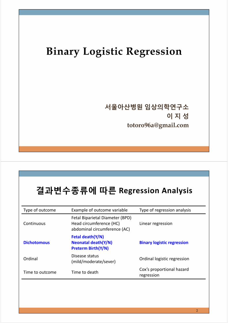
결과변수종류에따른 Regression Analysis

2

Type of outcome Example of outcome variable Type of regression analysis

ContinuousFetal Biparietal Diameter (BPD)Head circumference (HC)abdominal circumference (AC)

Linear regression

DichotomousFetal death(Y/N)Neonatal death(Y/N)Preterm Birth(Y/N)

Binary logistic regression

OrdinalDisease status (mild/moderate/sever)

Ordinal logistic regression

Time to outcome Time to deathCox’s proportional hazard  regression

Binary Logistic Regression

3

Example: Age and coronary heart disease (CHD)

4

Source: Colton. Statistics in Medicine (1974)

Scatter plot

5

6

Table 1. Prevalence (%) of CHD according to age group

7

Logistic Distribution

로지스틱 회귀모형

8

With the logistic transformation, we are fitting the “model” to the data better.

P(CHD=Yes) = 

P(CHD=Yes)

Transformed the “log odds” are linear.

9

P(CHD=Yes) 1 P(CHD=Yes)  = 

P(CHD=Yes) 

1 P(CHD=Yes) 

Pr Y 1 X

⇔ lnY 1 X

1 Y 1 X ln X

로지스틱 모형에서 회귀계수 β1이 가지는 의미

10

독립변수 X가 범주형 변수(범주가 2개)인 경우(예: sex(f=0, m=1))

– female(X=0)이면, ln 0

– male(X=1)이면, ln 1

– 차이: ln - ln ⇔ OR = exp( )

변수 X가 연속형 변수인 경우

– X=x0이면, ln

– X=x0 +1 이면, ln 1 1

– 차이: ln( ( 1)) - ln( ( ))= ⇔ OR = exp( )

NINDS trial dataset

SPSS: Logistic regression

11

독립변수결과변수

NINDS trial dataset

SPSS: Logistic regression

12

Age가 Poor functional outcome에 미치는 영향을 평가 기술통계량

3mo mRS=‘2‐6’군의 평균 Age가 3mo mRS=‘0‐1’군보다 높다.

Age는 Poor functional outcome에 어느 정도로 영향을 미치는가? 

Example (1): 독립변수가연속형

13

14

결과변수가 두 범주(dichotomous) 인 경우.‐ Binary logistic regression 

결과변수가 순서형 (ordinal) 변수인경우.‐ Ordinal logistic regression

결과변수가 명목형(nominal) 다범주(polychotomous)인 경우. ‐ polychotomous logistic regression

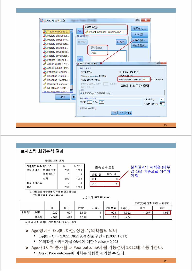
15

OR의 신뢰구간 출력

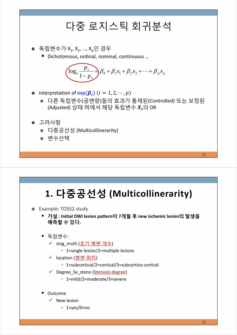
Age 행에서 Exp(B), 하한, 상한, 유의확률의 의미 Exp(B) = OR = 1.022, OR의 95% 신뢰구간 = (1.007, 1.037)

유의확률 = 귀무가설 OR=1에 대한 P‐value = 0.003

Age가 1세씩 증가할 때 Poor outcome이 될 가능성이 1.022배로 증가한다. 

Age가 Poor outcome에 미치는 영향을 평가할 수 있다. 

16

로지스틱 회귀분석 결과

분석결과의 해석은 (내부값=1)을 기준으로 해석해야 함.

※ Age가 10세씩 증가할 때의 OR을 계산하고자 한다면??

Age변수를 10으로 나눈 변수를 생성하여 그 변수로 로지스틱 회귀분석 실시

17

Age가 10세씩 증가할 때 Poor outcome이 될 가능성이1.242배로 증가한다. 

범주형 변수인 AGEGRP가 Poor functional outcome에 미치는 영향을 평가 30≤age≤39   agegrp = 1  40≤age≤49   agegrp = 2

50≤age≤59   agegrp = 3 60≤age≤69   agegrp = 4

70≤age agegrp = 5

Example (2): 독립변수가범주형

18

19

범주형 독립변수의 기준(참조) 범주 설정 Default: 마지막 범주 (가장 큰 숫자로 입력된 범

주 Agegrp의 경우, 연령대가 제일 낮은 그룹으로

기준범주로 설정 ‘처음’ 범주로 바꿈

AGEGRP(4)의 OR=4.019에 대한 해석 ‘30대’에 비해 ‘70세 이상’인 경우 Poor outcome이 될 가능성이 4.019배이다. 

OR의 95% 신뢰구간 = (1.308, 12.346), P‐value = 0.015

20

로지스틱 회귀분석 결과

표에서 코딩값이 모두 0인 범주가 기준범주임.

(1): Agegrp=2(40대) vs. Agegrp=1(30대)

(2): Agegrp=3(50대) vs. Agegrp=1(30대)

(3): Agegrp=4(60대) vs. Agegrp=1(30대)

(4): Agegrp=5(70세이상) vs. Agegrp=1(30대)

독립변수가 X1, X2, …, Xp인 경우 Dichotomous, ordinal, nominal, continuous …

Interpretation of exp 1, 2,⋯ , 다른 독립변수(공변량)들의 효과가 통제된(Controlled) 또는 보정된

(Adjusted) 상태 하에서 해당 독립변수 의 OR

고려사항 다중공선성 (Multicollinerarity)

변수선택

다중 로지스틱 회귀분석

21

ppx

xe xxx

p

p

221101log

Example: TOSS2 study 

가설 : Initial DWI lesion pattern이 7개월후 new ischemic lesion의발생을예측할수있다.

독립변수:

sing_multi (초기 병변 개수)

• 1=single lesion/2=multiple lesions

location (병변 위치)

• 1=subcortical/2=cortical/3=subcortico‐cortical

Degree_Sx_steno (Stenosis degree)

• 1=mild/2=moderate/3=severe

Outcome

New lesion 

• 1=yes/0=no

1. 다중공선성 (Multicollinerarity)

22

다중공선성(multicollinearity) check

23

X1X2

X3

New lesion

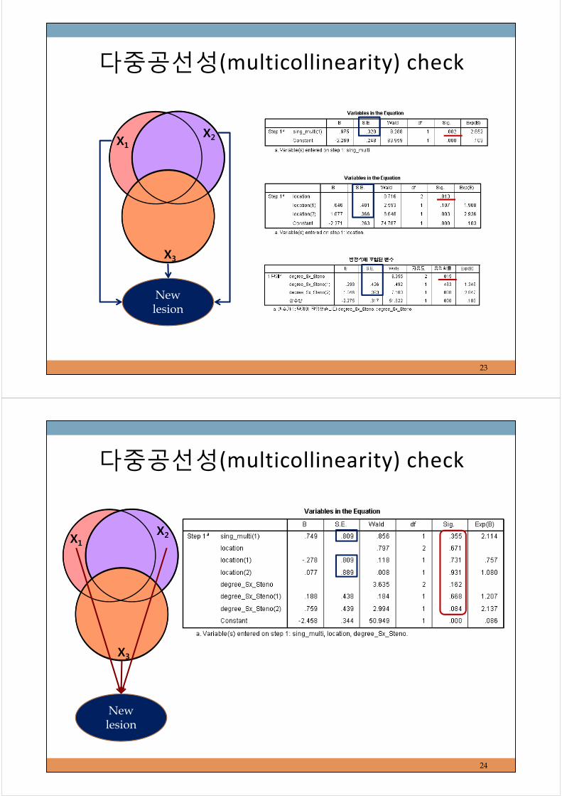
다중공선성(multicollinearity) check

24

X1X2

X3

New lesion

Method1: Correlation matrix for the parameters estimates output

다중공선성(multicollinearity) check

25

다중공선성(multicollinearity) check

26

Method2: Variance Inflation Factors (VIF) 

선형회귀분석의 공선성진단으로 확인가능

초기병변갯수와 병변위치간의 다중공선성 발생이 의심됨!!

두개의 독립변수가 서로 밀접하게 상관(혹은 연관)되어 있는 경우 혹은특정 독립변수가 나머지 독립변수들의 선형결합의 형태인 경우►다중 로지스틱 회귀모형에서 이들의 개별효과를 파악하기가 힘들

수 있음. 

►따라서 bivariate 분석에서는, 두 변수 모두 통계적으로 유의하게 나타났어도, 다중 로지스틱 회귀모형에 이 두 변수를 동시에 포함하였을 경우, 둘 다 종속변수와 관련이 없는 것으로 나타날 수 있음.

특정 변수들 사이에 공선성이 존재한다면 다중 로지스틱 회귀분석에서의 이들의 표준오차는 각각의 bivariate 분석에서 나타난 표준오차에 비해 상당히 클 것임. 

다중공선성 문제에 관한 가장 쉬운 해결방법은 해당 변수들 중 하나를모형에서 제외하는 것임.

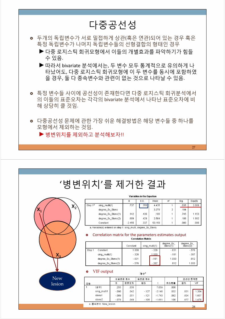
►병변위치를 제외하고 분석해보자!!

다중공선성

27

‘병변위치’를 제거한 결과

28

X1X2

X3

New lesion

Correlation matrix for the parameters estimates output

VIF output

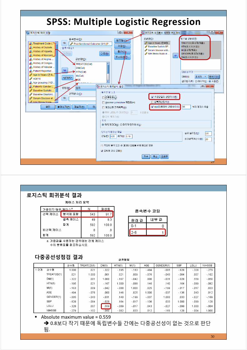
SPSS: Multiple Logistic Regression

29

30

로지스틱 회귀분석 결과

다중공선성점검 결과

Absolute maximum value = 0.559 0.8보다 작기 때문에 독립변수들 간에는 다중공선성이 없는 것으로 판단됨.

31

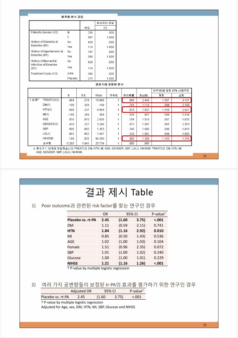
1) Poor outcome과 관련된 risk factor를 찾는 연구인 경우

2) 여러 가지 공변량들이 보정된 tr‐PA의 효과를 평가하기 위한 연구인 경우

결과 제시 Table 

32

OR 95% CI P‐value†

Placebo vs. rt‐PA 2.45 (1.60 3.75) <.001

DM 1.11 (0.59 2.11) 0.741

HTN 1.84 (1.16 2.92) 0.010

MI 0.85 (0.50 1.43) 0.536

AGE 1.02 (1.00 1.03) 0.104

Female 1.51 (0.96 2.35) 0.072

SBP 1.01 (1.00 1.02) 0.240

Glucose 1.00 (1.00 1.01) 0.229

NIHSS 1.21 (1.16 1.26) <.001† P‐value by multiple logistic regression

Adjusted OR 95% CI P‐value†

Placebo vs. rt‐PA 2.45 (1.60 3.75) <.001

† P‐value by multiple logistic regressionAdjusted for Age, sex, DM, HTN, MI, SBP, Glucose and NIHSS

로지스틱 회귀분석시 주의사항

로지스틱 회귀분석에서 OR값및 표준오차 값이 이상하게크게(혹은 작게) 나올 경우 해당 독립변수와 종속변수간의교차표를 꼭 확인해볼 것