behavioral/systems/cognitive ...nba.uth.tmc.edu/homepage/cnjclub/2011...

Behavioral/Systems/Cognitive

Multisensory Calibration Is Independent of Cue Reliability

Adam Zaidel, Amanda H. Turner, and Dora E. AngelakiDepartment of Anatomy and Neurobiology, Washington University School of Medicine, St. Louis, Missouri 63110

Multisensory calibration is fundamental for proficient interaction within a changing environment. Initial studies suggested a visual-dominant mechanism. More recently, a cue-reliability-based model, similar to optimal cue integration, has been proposed. However, amore general, reliability-independent model of fixed-ratio adaptation (of which visual dominance is a subcase) has never been tested.Here, we studied behavior of both humans and monkeys performing a heading-discrimination task. Subjects were presented with eithervisual (optic-flow), vestibular (motion-platform), or combined (visual–vestibular) stimuli and required to report whether self-motionwas to the right/left of straight ahead. A systematic heading discrepancy was introduced between the visual and vestibular cues, withoutexternal feedback. Cue calibration was measured by the resulting sensory adaptation. Both visual and vestibular cues significantlyadapted in the direction required to reduce cue conflict. However, unlike multisensory cue integration, cue calibration was not reliabilitybased. Rather, a model of fixed-ratio adaptation best described the data, whereby vestibular adaptation was greater than visual adapta-tion, regardless of relative cue reliability. The average ratio of vestibular to visual adaptation was 1.75 and 2.30 for the human and monkeydata, respectively. Furthermore, only through modeling fixed-ratio adaptation (using the ratio extracted from the data) were we able toaccount for reliability-based cue integration during the adaptation process. The finding that cue calibration does not depend on cuereliability is consistent with the notion that it follows an underlying estimate of cue accuracy. Cue accuracy is generally independent of cuereliability, and its estimate may change with a much slower time constant. Thus, greater vestibular versus visual (fixed-ratio) adaptationsuggests lower vestibular versus visual cue accuracy.

IntroductionIntegration of input from multiple sensory sources is required forcoherent perception and adept interaction with the environment.However, inherent noise and the probabilistic nature of oursenses make this task particularly challenging (Knill and Pouget,2004). Hence, the brain requires a proficient strategy for multi-sensory integration. Optimal integration schemes predict thatmultiple sensory cues should be weighted in accordance withtheir relative reliabilities, such that reliable cues are more influ-ential than less reliable cues (Yuille and Bulthoff, 1996; Jacobs,1999; Landy and Kojima, 2001). Indeed, a number of paradigmshave demonstrated reliability-based cue combination (RBCC)when integrating multisensory input (Ernst and Banks, 2002; vanBeers et al., 2002; Alais and Burr, 2004).

Reliability-based cue combination is considered optimal inthat it maximizes precision (synonymous here with reliability;defined by the inverse variance). Nonetheless, it may not accountfor accuracy, agreement between perception and the environ-ment. If, for example, a sensory cue is biased, reliability-based cuecombination may result in a biased perception (Watt et al., 2005).

Although there are circumstances in which reliability-based cuecombination may still be beneficial even with biased cues (Scarfeand Hibbard, 2011), cue calibration would enhance the accuracyof multisensory perception. However, without external feedback,it may not be possible to assess the accuracy of a sensory system.In this case, the best the brain can do is detect the relative biasbetween different sensory systems. Given a systematic discrep-ancy, sensory cues may undergo mutual calibration to achieve“internal consistency” (not to be confused with “external accu-racy”; Burge et al., 2010).

Several groups have suggested a reliability-based model formultisensory calibration, whereby the extent of adaptation isdetermined by the relative reliability of each cue (Ghahramaniet al., 1997; Witten and Knudsen, 2005; Burge et al., 2010).Reliability-based adaptation (RBA) seems a logical extensionof reliability-based cue combination, particularly because thetraditional view of visual-dominant adaptation (VDA) (Rockand Victor, 1964) has been challenged by accounts of visualrecalibration (Lewald, 2002; Atkins et al., 2003). However, themost reliable cue might not always be the most accurate (Ernstand Di Luca, 2011). Furthermore, there is still evidence for visual-dominant effects (Knudsen, 2002; Spence, 2009). In fact, visual-dominant adaptation is only a subcase of a generalized fixed-ratioadaptation (FRA) model, whereby cues adapt toward one an-other at a fixed ratio regardless of cue reliability (possibly accord-ing to the underlying estimates of cue accuracy), yet a model offixed-ratio adaptation has never been quantitatively comparedwith reliability-based adaptation. Hence, the manner, principles,and extent to which multiple sensory systems adapt to one an-other remains fundamentally missing.

Received June 1, 2011; revised July 28, 2011; accepted Aug. 8, 2011.Author contributions: D.E.A. designed research; A.Z. and A.H.T. performed research; A.Z. analyzed data; A.Z. and

D.E.A. wrote the paper.The authors declare no competing financial interests.This work was supported by NIH Grants EY019087, DC007620, and 5-T32-EY13360-10, and by the Edmond and

Lily Safra Center for Brain Sciences at the Hebrew University of Jerusalem. We thank Chris Fetsch for his help withpilot experiments and Jason Arand and Heide Schoknecht for their help with data collection.

Correspondence should be addressed to Adam Zaidel, Washington University, School of Medicine, Department ofAnatomy and Neurobiology, 660 South Euclid Avenue, Box 8108, St. Louis, MO 63110. E-mail: [email protected].

DOI:10.1523/JNEUROSCI.2732-11.2011Copyright © 2011 the authors 0270-6474/11/3113949-14$15.00/0

The Journal of Neuroscience, September 28, 2011 • 31(39):13949 –13962 • 13949

Perception of self-motion and heading direction relies partic-ularly on visual and vestibular input (Guedry, 1974; Warren andHannon, 1988; Ohmi, 1996). We have shown previously in aheading discrimination task that visual–vestibular integrationprimarily follows reliability-based cue combination for both hu-mans and monkeys (Gu et al., 2008; Fetsch et al., 2009). In thisstudy, we probe the nature of visual–vestibular calibration byintroducing a systematic discrepancy between visual and vestib-ular cues, in the same heading discrimination task, and assessingthe resulting perceptual adaptation of the individual cues.

Materials and MethodsSeparate experiments were performed on humans and monkeys. Detailsof the apparatus, stimuli, and basic task design, published previously forboth humans (Fetsch et al., 2009; Gu et al., 2010; MacNeilage et al., 2010)and monkeys (Gu et al., 2007, 2008, 2010; Fetsch et al., 2009), are brieflysummarized below together with the methods specific for this study. Foradditional details, see previous studies.

Human experimentNine human subjects (four male) participated in this study. All signedinformed consent, and the study was approved by the Washington Uni-versity Human Research Protection Office. Subjects were seated com-fortably in a cockpit-style chair and restrained safely with a five-pointracing harness. Each subject wore a custom-made thermoplastic maskthat was attached to the back of the chair for head stabilization. The chair,a three-chip DLP projector (Galaxy 6; Barco), and a large projectionscreen were all mounted on a motion platform (6DOF2000E; Moog) toprovide synchronized visual and vestibular input. The projection screen(149 ! 127 cm) was located "70 cm in front of the eyes, subtending avisual angle of "94° ! 84°. Subjects were enclosed in a black aluminumsuperstructure, such that only the display screen was visible in a darkenedroom, and wore active three-dimensional glasses (CrystalEyes 3; RealD)to provide stereoscopic depth cues. The field of view through the glasseswas "70° ! 90°.

The subjects’ task was to discriminate heading direction (two-alternativeforced choice, right or left of straight ahead), after presentation of asingle-interval stimulus. Subjects were instructed to focus on a centralfixation point throughout the duration of the trial. Trials were initi-ated, and choice selection was reported via button press on a hand-held unit. Subjects received trial timing-related feedback throughheadphones. However, no feedback about correct or incorrect choiceswas provided.

The stimulus presented was either vestibular-only, visual-only, or si-multaneously combined vestibular and visual cues. The vestibular-onlystimulus was inertial motion of the platform in darkness (no optic-flowcues). The visual-only stimulus was optic-flow motion simulation, with-out inertial motion of the platform. The combined vestibular and visualstimulus comprised inertial motion in conjunction with synchronizedoptic flow. Although additional cues, such as proprioception and so-matosensation, could also be present during inertial motion, we refer tothis condition as “vestibular ” because primate performance dependsstrongly on intact vestibular labyrinths (Gu et al., 2007). The stimulusvelocity followed a 4 ! Gaussian profile with duration of 1 s and totaldisplacement of 13 cm. Peak velocity was 0.35 m/s, and peak accelerationwas 1.4 m/s 2.

The optic flow simulated self-motion of the subject through arandom-dot cloud. Visual cue reliability was varied by manipulating themotion coherence of the optic-flow pattern, i.e., percentage of dots mov-ing coherently. Three levels of coherence were used: high (100% coher-ence), medium (50% coherence), and low. The latter was subject specific,determined such that the subject’s visual threshold was larger than thesubject’s vestibular threshold. Vestibular reliability was fixed throughoutthe trials. For each session, the actual reliability ratio (RR) of the visual/vestibular cues, extracted from single-cue psychophysical data, was usedfor analysis (see below, Data analysis). Subjects were given several prac-tice sessions before data collection to familiarize themselves with the

experiment and to extract subject-specific coherence levels for low visualreliability.

Seven heading directions were tested: straight ahead and three to eachside. Heading angles were varied in small steps, spaced approximatelylogarithmically around straight ahead, and presented using the methodof constant stimuli. The eccentricities of the heading angles were changedin accordance with the level of visual coherence, such that low visualcoherence trials had larger heading direction angles. This was necessaryto span the psychometric region of interest adequately, because lowercoherences yield a wider psychometric curve.

Each experimental session consisted of three consecutive blocks, asfollows.

Pre-adaption block. A pre-adaptation block comprised cues from onlya single (visual-only/vestibular-only) modality, interleaved. The result-ing psychometric curves were used to deduce the baseline bias and indi-vidual reliability of each modality for the subjects. This block comprised[10 repetitions] ! [2 stimuli (visual-only/vestibular-only)] ! [7 headingangles] # 140 trials.

Adaptation block. In this block, only combined visual–vestibular cueswere presented. Across the trials, a discrepancy between the visual andvestibular cues was introduced incrementally: $ # %2°, 4°, 6°, 8°, 10°,and then held at %10° for the remainder of the block. The discrepancywas introduced incrementally to prevent awareness of the subject. Byconvention, the sign of $ indicated the orientation of discrepancy: pos-itive $ represented an offset of the vestibular cue to the right and visualcue to the left; negative $ indicated the reverse. Only one discrepancyorientation, positive or negative, was used per session. Eight repetitionswere run for each $ increment, and an additional seven repetitions wererun for maximum $ (%10°), resulting in [(8 ! 5 & 7) repetitions] ! [7heading angles] # 329 trials.

Post-adaptation block. During this block, adaptation of the individual(visual/vestibular) cues was measured by single-cue trials, similar to thepre-adaptation block. The single-cue trials were interleaved withcombined-cue trials (with $ # %10°, as in the end of the adaptationblock) to maintain the adaptation while it was measured. This blockcomprised [10 repetitions] ! [3 stimuli (visual-only/vestibular-only/combined)] ! [7 heading angles] # 210 trials.

In total, there were 679 trials in a session, which typically lasted "60min. Subjects participated in 12 such sessions: [2 session repeats] ! [3coherences (high/med/low)] ! [2 deltas (positive or negative)]. For onesubject, low-coherence data were not collected; for another, medium-coherence data were not collected. Hence, these two subjects participatedin eight sessions. Sessions were sorted by low, medium, and high reliabil-ity ratio using the actual cue thresholds (see below, Data analysis). To testwhether there was any influence of measuring both cues in the samesession, three subjects participated in eight additional sessions duringwhich cues were tested individually: [2 cues (visual/vestibular)] ! [2coherences (high/low)] ! [2 $ (positive or negative)]. The single-cueprotocol was identical to the standard protocol, but all single-cue trials ofthe other (nontested) cue were removed. Single-cue trials of the cuebeing tested and combined-cue trials remained unchanged. There wereno observable differences between the results of single-cue sessions andstandard sessions. The data presented here are from the standard sessionsonly. In total, n # 100 experimental sessions were analyzed from the ninehuman subjects in this study.

Monkey experimentFour male rhesus monkeys (Macaca mulatta) participated in the study.All procedures were approved by the Animal Studies Committee atWashington University. Monkeys were head fixed and seated in a pri-mate chair that was anchored to a motion platform, identical to theplatform used in the human experiment. Also mounted on the platformwere a stereoscopic projector (Mirage 2000; Christie Digital Systems), arear-projection screen, and a magnetic field coil (CNC Engineering) formeasuring eye movements (Judge et al., 1980). The projection screen(60 ! 60 cm) was located "30 cm in front of the eyes, subtending a visualangle of "90° ! 90°. Monkeys wore custom stereo glasses made fromWratten filters (red #29 and green #61; Eastman Kodak), which enabled

13950 • J. Neurosci., September 28, 2011 • 31(39):13949 –13962 Zaidel et al. • Multisensory Calibration Follows a Fixed Ratio

rendering of the visual stimulus in three dimensions as red– greenanaglyphs.

As in the human experiment, the monkeys’ task was to discriminateheading direction (two-alternative forced choice, right or left of straightahead), after presentation of a single-interval stimulus. The monkeyswere required to fixate on a central target during the stimulus and thenreport their choice by making a saccade to one of two choice targets(right/left) illuminated at the end of the trial. Like in the human experi-ment, the stimulus presented was either vestibular-only, visual-only, orsimultaneously combined vestibular and visual stimuli. The stimulusvelocity followed a 4 ! Gaussian profile with the same parameters as thehuman experiment: duration of 1 s; total displacement of 13 cm; peakvelocity of 0.35 m/s; and peak acceleration of 1.4 m/s 2. Ten headingdirections were tested: five to each side. Heading angles were varied insmall, logarithmically spaced steps around straight ahead and presentedusing the method of constant stimuli.

The optic flow simulated self-motion of the monkey through arandom-dot cloud. Visual cue reliability was varied by manipulating themotion coherence of the optic-flow pattern, i.e., percentage of dots mov-ing coherently. Two levels of coherence were used: high (100% coher-ence) and low. Low coherence was monkey specific, determined suchthat the monkey’s visual threshold was larger than its vestibular thresh-old. Vestibular reliability was fixed throughout the trials. For each ses-sion, the actual reliability ratio of the visual/vestibular cues extractedfrom the data was used for analysis (see below, Data analysis).

The monkey experimental session was similar to that of the humans,also comprising pre-adaptation, adaptation, and post-adaptation blocks.However, at the end of a trial, monkeys were either rewarded or notrewarded with a portion of water/juice. Reward strategy was manipulatedso as not to interfere with the adaptation, as described below.

Pre-adaption block. The pre-adaptation block comprised visual-only/vestibular-only/combined cues, interleaved. For some sessions, the com-bined stimulus was excluded. The monkey was rewarded for correctchoices 95% of the time and not rewarded for incorrect choices. The 95%correct reward rate was used to accustom the monkey to not gettingrewarded all of the time, as was the case in the post-adaptation blockdescribed below. This block was used to deduce the baseline bias andindividual reliability (psychometric curve) of each modality for the mon-keys. It comprised [10 repetitions] ! [3 stimuli (visual-only/vestibular-only/combined)] ! [10 heading angles] # 300 trials. When thecombined stimulus was excluded, the block comprised 200 trials.

Adaption block. In the adaptation block, only combined visual–ves-tibular cues were presented. A discrepancy of $ # %10° was introducedbetween the visual and vestibular cues for the entire duration of theblock. Like the human experiments, the sign of $ indicated the orienta-tion of discrepancy: positive $ represented an offset of the vestibular cueto the right and visual cue to the left; negative $ indicated the reverse.Only one discrepancy orientation was used per session. During thisblock, the monkey did not make direction choices. Rather, it was re-warded only for keeping its eyes fixated on the central target for theduration of the trial. Choice targets were not presented at the end of thetrial. That way, the reward did not generate any bias for visual/vestibularcues, and perceptual adaptation reflects the mutual influence of the mo-dalities on one another. This block typically comprised [50 repetitions]! [10 heading angles] # 500 trials.

Post-adaption block. During the post-adaptation block, the adaptationof the individual (visual/vestibular) modalities was measured by single-cue trials, interleaved with the combined-cue trials (with $ # %10° as inthe adaptation block). The combined-cue trials were run in the same wayas in the adaptation block: rewarded by eye-fixation alone with no head-ing direction choice. They were included to retain adaptation. The prob-ability of reward for single-cue trials worked slightly differently from thepre-adaptation block so as not to perturb the adaptation. When thesingle-cue trial was at a heading angle, such that if it were a combined-cuetrial the other modality would be to the same direction (right/left), themonkey was rewarded as in the pre-adaptation block (95% probabilityreward for correct choices; no reward for incorrect). If however, the othermodality would have been to the opposite side, a reward was given proba-bilistically (70%, no matter what the choice). This value was chosen

because it approximately represents the correct choice rate in a normalheading discrimination task. This block typically comprised [20 repeti-tions] ! [3 stimuli (visual-only/vestibular-only/combined)] ! [10heading angles] # 600 trials. At least 10 repetitions were required in thisblock for the session to be included in the study.

A typical session comprised "1400 trials ("2.5 h in total) and was runat either high/low coherence, with either positive/negative $. Sessionswere sorted by low, medium, and high visual to vestibular RR using theactual cue thresholds (see below, Data analysis). For each monkey, therewere at least four repetitions for each discrepancy orientation (positiveand negative $) at both high and low RR. Medium RR data were of asimilar quantity. Monkey C was missing three of the eight high RR ses-sions because 100% visual coherence did not reliably result in high RR,and coherence cannot be increased '100%. In total, n # 108 experimen-tal sessions were analyzed from the four monkeys in this study. Onemedium RR data point had a large vestibular shift ('10°), so it wasexcluded from Figures 4 and 5. However, it was in line with the resultsand was included in all data analyses and regressions.

Monkeys were able to perform “fixation-only” trials (as presented inthe second and third block) interchangeably with the standard “heading-discrimination” trials (as presented in the first and third block) withoutany difficulty, and they did not need to be cued in advance which type oftrial they were doing. This is because they were required to fixate duringthe stimulus regardless of the type of trial. After the stimulus, either themonkey was rewarded for fixating up until this point (fixation-only tri-als) or the central fixation point would disappear and choice targetswould appear on the screen (heading-discrimination trials) cueing themonkey that it has to make a selection.

Data analysisData analysis was performed with custom software using Matlab R2006a(MathWorks) and the psignifit toolbox for Matlab (version 2.5.6; Wich-mann and Hill, 2001a,b). Psychometric plots were defined as the propor-tion of rightward choices as a function of heading angle and calculated byfitting the data with a cumulative Gaussian distribution function. Foreach experimental session, separate psychometric functions were con-structed for visual and vestibular cues before and after adaptation. Thepsychophysical threshold and point of subjective equality (PSE) were theSD (!) and mean ("), respectively, deduced from the fitted distributionfunction. The PSE represents the heading angle of equal right/left choiceproportion, i.e., perceived straight ahead, also known as the bias. Visual/vestibular adaptation was measured as the difference between the pre-and post-adaptation PSEs.

For (2% of the post-adaptation distribution functions, there was onlyone data point that was not 0 or 1 (there were no distribution functions inwhich all data points were either 0 and 1). This resulted from a large PSEshift to a region where the curve was sparsely sampled. For these sessions,it was difficult to determine the SD of the cumulative Gaussian. Hence,the pre-adaptation SD was used as a Bayesian “prior” for fitting thepost-adaptation psychometric plot. The prior was a raised cosine func-tion that touched 0 at the 95% confidence limits of the pre-adaptationSD.

The RR was defined as the ratio of the visual/vestibular reliabilities andcalculated for each session individually. Cue reliability was computed bytaking the inverse of the threshold squared, using the geometric mean ofthe pre-adaptation and post-adaptation thresholds extracted from thefitted psychometric curves. For both human and monkey experiments,the data were divided into three RRs: low RR (RR # 2.5 )1), medium RR(2.5 )1 ( RR ( 2.5), and high RR (RR $ 2.5). Because behavioral per-formance could change over time as a result of a “practice” effect, we didnot assume that RRs were equal across sessions of the same subject withthe same coherence. We therefore calculated the RR for each sessionindividually.

When calculating a linear regression between two dependent variables,each containing uncertainty/noise in their measurements, a type II re-gression was used (the perpendicular distances between the data pointsand the regression line were minimized).

Zaidel et al. • Multisensory Calibration Follows a Fixed Ratio J. Neurosci., September 28, 2011 • 31(39):13949 –13962 • 13951

ResultsBehavioral data of the nine human subjects who participated inthe human experiment and four monkeys from the monkeyexperiment were analyzed and are presented in this study.Before presenting the data, we first introduce a brief theoret-ical background on which data analysis was based, followed bysimulation of the experimental outcome according the theo-retical predictions.

Theoretical framework for multisensory adaptation in theabsence of external feedbackWhen presented with an environmental stimulus S, individualsensors (e.g., A and B) will estimate S based on their individual

estimator functions: SA # fA(S) and SB # fB(S), where SA and SB

represent their respective estimates. The “internal consistency”hypothesis predicts that, if the expectancies of the estimates,

E*SA) and E(SB), are not equal, then (in the absence of externalfeedback) estimator functions will adapt toward one another toachieve equality and internal consistency. Cue-adaptation direc-tion will be dependent on the discrepancy, $, of the cues:

$ % SB & SA, (1)

such that fA will adapt proportional to &$ and fB will adaptproportional to )$. However, the rate and extent of adaptationmay be different for the cues. How the two estimator functionsadapt toward one another can follow either one of the followingprinciples.

Bayesian prediction of multisensory adaptationThe model of RBA predicts that the extent to which each estima-tor function adapts is dependent on the reliabilities of the cues.This was described by Ghahramani et al. (1997) as the weighted $rule:

'fA*S+ % ( ) wB ) $,'fB*S+ % ( ) wA ) * & $+, (2)

where 'fA and 'fB are the additive changes to the cue estimators,( is the adaptation rate (small positive constant), and wA and wB

are the weights calculated by the cues’ relative reliabilities:

wA %rA

rA * rB

wB %rB

rA * rB,

(3)

and cue reliability (rA and rB) is defined as the inverse variance:

rA % 1/!A2

rB % 1/!B2 . (4)

Note that wA & wB # 1 and that the weights for multisensoryadaptation are complementary to those used for multisensoryintegration. Namely, for cue integration, wA is used to weight theestimate of cue A and wB is used to weight the estimate for cue B.However, for cue adaptation, the extent of the adaptation of cue Ais determined by wB, and the extent of adaptation of cue B isdetermined by wA. This is because the more reliable a cue, thehigher it will be weighted during integration and the less it willundergo calibration (and vice versa).

Fixed-ratio prediction of multisensory adaptationFRA predicts that cues adapt at a fixed ratio regardless of relativereliability. Thereby, estimator functions will adapt according tothe following:

'fA*S+ % ( ) $,'fB*S+ % C ) ( ) ( & $), (5)

where C is a constant. A subcase of FRA is VDA, in which the ratioof non-visual cue adaptation to visual adaptation tends to infinity(only the non-visual cue adapts).

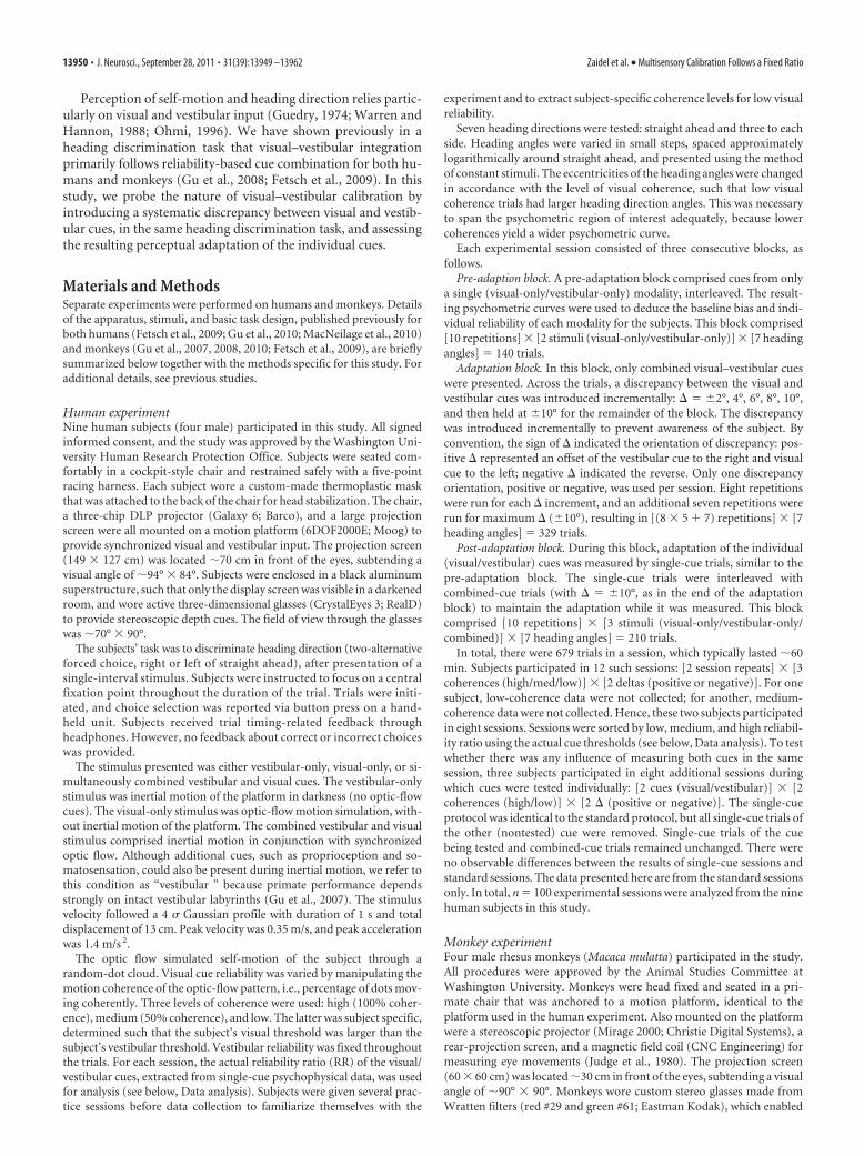
Visual–vestibular adaptation: simulationTo explain the expected outcome of visual–vestibular adaptation,we simulated performance for the task used in this study accord-ing to the theoretical framework presented above. Two models ofadaptation were simulated: RBA and VDA. The simulation par-adigm was a replica of the human experimental protocol, whichwas similar to the monkey protocol except for a few slightdifferences as detailed in Materials and Methods. Psychophys-ical discrimination of heading direction was simulated in a two-alternative forced-choice task (right or left of straight ahead).Like the actual experiments, the stimulus comprised eithervestibular-only (inertial-motion), visual-only (optic-flow), or si-multaneously combined vestibular and visual cues. Simulatedpsychometric curves depict the ratio of rightward choices as afunction of stimulus heading direction (Fig. 1, middle three col-umns). The PSE was extracted from the fitted Gaussian cumula-tive distribution function and represents the estimate of a cue forstraight ahead.

All baseline (pre-adaptation) simulations were generated withPSE # 0, i.e., no heading-direction bias. Precision of individualpsychometric curves was controlled by setting the variance of theunderlying Gaussian functions (Eq. 4). To induce a cue conflict, adiscrepancy between the visual and vestibular headings was in-troduced incrementally: $ # 2°, 4°, 6°, 8°, 10°. Cue adaptationwas simulated according to RBA and VDA and measured by theresulting shift in the visual–vestibular PSEs. For these simula-tions, multisensory adaptation achieved internal consistency,namely, visual–vestibular PSEs shifted a combined 10° to cancelout the introduced $. We did not simulate the actual time courseof adaptation but rather the endpoint (from pre-adaptation topost-adaptation) according to the ratio of vestibular/visual adap-tation predicted by the models. The simulated shifts are pre-sented in Figure 1: vestibular pre-adaptation and post-adaptationpsychometric curves are presented in blue and cyan, respectively,and visual pre-adaptation and post-adaptation psychometriccurves are presented in red and magenta, respectively.

For RBA (Fig. 1A), both visual and vestibular cues shiftedtoward one another. The extent to which each cue shifted wasdependent on RR (ratio of visual to vestibular reliability). Visualand vestibular reliabilities were calculated according to Equation4, using the variances extracted from the fitted cumulative Gauss-ian functions. Three different RRs were simulated: when RR # 5,the vestibular cue shifted five times more versus visual (toprow); when RR # 1, both cues shifted equally (second row);and when RR # 1⁄5, the visual cue shifted five times moreversus vestibular (third row). For VDA (Fig. 1 B), only thevestibular curve shifted, whereas the visual curve did not shift.This happens regardless of RR.

The combined-cue responses during the adaptation block canprovide insight into the type of adaptation. However, analysis ofthese data first requires definition of the reference frame because


there is no absolute heading direction for the combined cue whenindividual cues are discrepant. In this study, the combined-cueaxis (0) was artificially defined by the heading midway betweenthe visual and vestibular cues. Hence, during the simulated adap-tation block, the visual and vestibular heading angles were &$/2and )$/2, respectively. As $ increased, the headings of both cuesbecame more eccentric but remained symmetric around thecombined cue 0. For each value of $, the combined psychometriccurve was calculated (Fig. 1, second column from the right). Thecombined-cue PSE was then extracted and plotted as a functionof $ (Fig. 1, rightmost column). Positive or negative combined-cue PSE values therefore indicate higher visual or vestibularweighting, respectively. PSE # 0 indicates equal weighting.

The combined plots presented here should therefore not bemistaken to represent a psychometric shift. In fact, according toboth model simulations (RBA and VDA), the combined-cue re-sponse does not shift, in world coordinates, during adaptation.Rather, the observed changes in combined PSE are attributable toincreasing $ and the concurrent increase in heading eccentricityof the individual cues. Why do both RBA and VDA not predict ashift in the combined cue? If cue combination and cue adaptationfollow the same model, then the combined cue will not shift. Thisis because, during cue adaptation, cues converge on the initial cuecombination. For example, (1) visual-dominant cue combina-tion always aligns the combined response with the visual cue;during VDA, only the vestibular cue adapts until it is aligned withthe visual cue. Hence, the combined cue will not change duringVDA. (2) During RBA, visual and vestibular cues shift accordingto the weights of Equation 3, the same weights used for RBCC.

Hence, the combined cue response will remain unchanged dur-ing RBA. If, however, different models were used for cue combi-nation and cue adaptation, the combined response would shiftduring adaptation. This issue is further discussed in the last sec-tion of Results.

Therefore, in this simulation, the slope of combined PSE ver-sus $ (Fig. 1, rightmost column) is simply an indication of cueweighting: a positive versus negative slope indicates higher visualversus vestibular weighting, respectively. A 0 slope indicatesequal weighting. For RBA, when RR # 5, the combined responsewas weighted more by the visual cue (positive slope; top row),when RR # 1⁄5, it was weighted more by the vestibular cue (neg-ative slope; third row), and when RR # 1, there was equal weight-ing (0 slope; second row). For VDA, the combined responsealways aligns with the visual cue (at &$/2). Hence, the combinedPSE versus $ always demonstrates the maximum slope, 1⁄2 (bot-tom row).

Visual–vestibular adaptation: examplesIn the simulation presented in Figure 1, a cue conflict of $ #&10° was used (vestibular cue offset to the right; visual to theleft). The predictions for $ # )10° (vestibular cue offset tothe left; visual to the right) are the same but with shifts in thereverse direction. In the actual experiments, both orientationsof $ were used. Hence, when analyzing the data, the predictedcue shifts for positive versus negative $ are equal but oppositein sign/direction.

Figure 2 shows representative psychophysical data from onehuman subject. Two experimental sessions are presented, for

Figure 1. Simulation of multisensory adaptation. Idealized behavioral responses in a heading discrimination task based on vestibular (Vest), visual (Vis), or both (combined) cues, according toRBA (A) and VDA (B). Psychometric plots (middle 3 columns) represent the simulated ratio of rightward choices, as a function of heading direction. Data (circles) were fitted with cumulative Gaussianfunctions (solid lines). Baseline performance is presented for vestibular and visual cues by the blue and red curves, respectively. After introducing a heading discrepancy ($ # 10°), vestibular andvisual cues adapted to cancel out the discrepancy (cyan and magenta post-adaptation curves, respectively). For RBA, cues shifted according to the visual versus vestibular RR, i.e., for RR # 5 (toprow), the vestibular cue shifted five times more than the visual cue; for RR # 1 (middle row), cues shifted equally; and for RR # 1⁄5 (bottom row), the visual cue shifted five times more than thevestibular cue. For VDA, the visual cue did not shift (pre-adaptation and post-adaptation curves are superimposed); only the vestibular cue shifted. This happens regardless of RR (RR # 1 was usedfor the example presented here). Dark to light shades of green show the combined-cue responses during adaptation, while gradually increasing $# 2°, 4°, 6°, 8°, 10°. The axis of the combined-cueaxis (0) is defined by the heading midway between the cues (schematics on the left). In the rightmost column, the combined-cue PSE is plotted as a function of $. Solid black lines representregressions through the origin. For RBA, regression slopes followed the RR: positive for higher visual weighting (top row), negative for higher vestibular weighting (third row), and 0 for equalweighting (second row). For VDA, the regression demonstrated maximal visual weighting (slope # 1⁄2; bottom row).


both possible orientations of cue conflict ($ # %10°). Motiondot coherence was 100%, and RR ' 1 for both examples (cuereliabilities were calculated using Eq. 4 and the fitted Gaussianfunctions). Cue shifts are presented here with 95% confidenceintervals for the PSE, calculated by bootstrapping the psychomet-ric curve: for $ # &10° (Fig. 2A), the vestibular PSE shifted from)0.3° [)0.9, 0.4] to 2.4° [1.6, 3.2], and the visual PSE shiftedfrom 0.9° [0.4, 1.5] to 0.1° [)0.4, 0.6]. For $ # )10° (Fig. 2B),the vestibular PSE shifted from )1.0° [)1.8, )0.2] to )3.0°[)4.4, )1.9], and the visual PSE shifted from 0.3° [)0.3, 1.0] to1.8° [1.0, 2.8].

For both examples, visual and vestibular psychometric curvesshifted in the direction required to reduce cue conflict (similar tothe RBA simulation; Fig. 1A). However, unlike the simulations,internal consistency was not achieved: vestibular & visual cuesshifted only a combined 2.7° & 0.8° # 3.5° for the example inFigure 2A and 2.0° &1.5° # 3.5° for the example in Figure 2B, lessthan the introduced discrepancy of 10°. The (absolute) ratio ofvestibular/visual PSE adaptation was 2.7°/0.8° # 3.4 for the ex-ample in Figure 2A and 2.0°/1.5° # 1.3 for the example in Figure2B compared with the RR predictions of 1.9 and 1.1, respectively.The positive (Fig. 2A) and negative (Fig. 2B) slope of the com-bined PSE versus $ indicate higher weighting of the visual cue, asexpected for RR ' 1.

Similarly, Figure 3 shows representative psychophysical dataof two experimental sessions from one monkey ($ # %10°).Motion dot coherence was 100% and RR ' 1 for both examples(cue reliabilities were calculated using Eq. 4 and the fitted Gauss-ian functions). Cue shifts are presented here with 95% confidenceintervals for the PSE, calculated by bootstrapping the psychomet-ric curve: for $ # &10° (Fig. 3A), the vestibular PSE shifted from0.5° [)1.4, 2.3] to 4.0° [2.7, 5.7], and the visual PSE shifted from)0.3° [)0.9, 0.7] to )0.5° [)1.1, 0.0]. For $ # )10° (Fig. 3B),the vestibular PSE shifted from 0.6° [)0.9, 2.2] to )6.6° [)8.7,

)4.9], and the visual PSE shifted from 0.8° [)0.3, 1.7] to 2.3°[1.8, 3.0].

Similar to the human examples, visual and vestibular psy-chometric curves shifted in the direction required to reducecue conflict but did not achieve internal consistency: the com-bined vestibular & visual shift was 3.5° & 0.3° # 3.8° for theexample in Figure 3A and 7.2° & 1.6° # 8.6° for the example inFigure 3B. The (absolute) ratio of vestibular to visual adapta-tion was 3.5°/0.3° # 11.7 for the example in Figure 3A and7.2°/1.6° # 4.5 for the example in Figure 3B compared with theRR predictions of 15.9 and 5.7, respectively. There were nobehavioral responses during the adaptation block of the mon-key experiments because of experimental constraints (themonkeys were rewarded for fixation only during the adapta-tion block and therefore did not make heading selections; seeMaterials and Methods).

Cue adaptation ratio changes with cue reliabilityTo quantify the results across experimental sessions, we first usedan analysis based on cue adaptation ratio, as previously done byBurge et al. (2010). Because visual and vestibular cues are ex-pected to adapt toward one another, their psychometric shiftsshould always be opposite in direction. Hence, the ratio of ves-tibular/visual shift should always be negative. Also, shift direc-tions should reverse for positive versus negative $. Therefore, asingle data point, plotted as the vestibular versus visual psycho-metric curve shift, is expected to lie in quadrant II of the Cartesianplane (top left: positive vestibular shift, negative visual shift) forpositive $ and in quadrant IV (bottom right: negative vestibularshift, positive visual shift) for negative $. Hence, a regression lineof pooled vestibular versus visual shifts is expected to have nega-tive slope, with two possible extremes: a vertical line would indi-cate only vestibular (and no visual) shift, and a horizontal linewould indicate only visual (and no vestibular) shift.

Figure 2. Example of human multisensory adaptation. Two example sessions of visual–vestibular adaptation, from one human subject, are presented. For both sessions, visual coherence #100% (RR ' 1). Plotting conventions are the same as Figure 1. However, opposite visual–vestibular heading discrepancies ($) were used for the two examples: in A, $ was positive. Hence, resultscan be compared directly with the simulation results of Figure 1 (which also used positive $). In B, $ was negative. Hence, shifts are expected in the reverse direction. R 2 $ 0.9 for all psychometricfits. Vis, Visual; Vest, vestibular.


RBA predicts that the magnitude of the visual to vestibular shiftratio should be dependent on RR. Specifically, for high RR, the ves-tibular shift is expected to be larger in magnitude than the visualshift, i.e., near-vertical regression line. For low RR, the visual shift isexpected to be larger in magnitude than the vestibular shift, i.e.,near-horizontal regression line. Finally, for medium RR, compara-ble magnitudes are expected, i.e., regression line with slope of ap-proximately )1. In contrast, FRA predicts that the slope will be fixedaccording to a constant adaptation ratio, such that the same slopewould be seen for low, medium, and high RR. A special case of FRAis VDA, that predicts a vertical regression line, only vestibular adap-tation, regardless of RR.

To test which model best depicts cue adaptation, the data weresorted by low, medium, and high RR, and the vestibular versus visualshifts were plotted (Fig. 4). The results clearly contradicted the VDAmodel, because visual shifts were observed. In fact, for both the hu-man (Fig. 4A) and the monkey (Fig. 4B) data, there seemed to be aninfluence of RR on cue adaptation, suggestive of RBA and not FRA.As predicted by RBA, high RR data approach a vertical line (Fig. 4,third column; especially for the monkey data) versus low RR data,which approach a horizontal line (Fig. 4, first column). Such conclu-sions would be similar to those of Burge et al. (2010), who concludedthat visual–haptic cue adaptation follows the RBA model. However,these results need to be treated with caution because of the largechanges in variability observed for different RRs. Specifically, vari-ability of visual PSE shifts increased with decreasing RR, as discernedby the distribution of data along the x-axis (Fig. 4; these changes invariability are quantified below and in Fig. 5, rightmost column). Infact, data variability itself can strongly influence the orientation ofthe regression lines (we elaborate on this point in Discussion).Hence, these plots are not adequate to conclude that cue adaptationfollows RBA.

If cue adaptation were to achieve internalconsistency, then the absolute sum of cueshifts would equal 10°. When summing theabsolute visual and vestibular PSE shifts(histograms in Fig. 4), it is very apparentthat cue adaptation does not reach internalconsistency. In fact, for almost all of thedata, the sum of PSE shifts was (10°. This isnot surprising given the limited length ofour experiments. Visual inspection of thecue-shift plots from Burge et al. (2010) indi-cate the same to be true for visual–hapticadaptation.

Complete adaptation (internal consis-tency) is actually not a requirement to testthe models. This is because, according to thetheoretical framework presented above, theratio of cue adaptation would be the sameafter partial adaptation as for complete ad-aptation. However, because of the largevariability in cue shifts (as described above),the adaptation ratio may not adequatelyrepresent individual sessions. Furthermore,cues sometimes shifted in the “unexpected”direction (marked by the gray regions in Fig.4; especially the visual cue at low RR).Therefore, to gain additional insight into theeffects of cue reliability on adaptation, wenext analyzed adaptation magnitude sepa-rately for visual and vestibular cues.

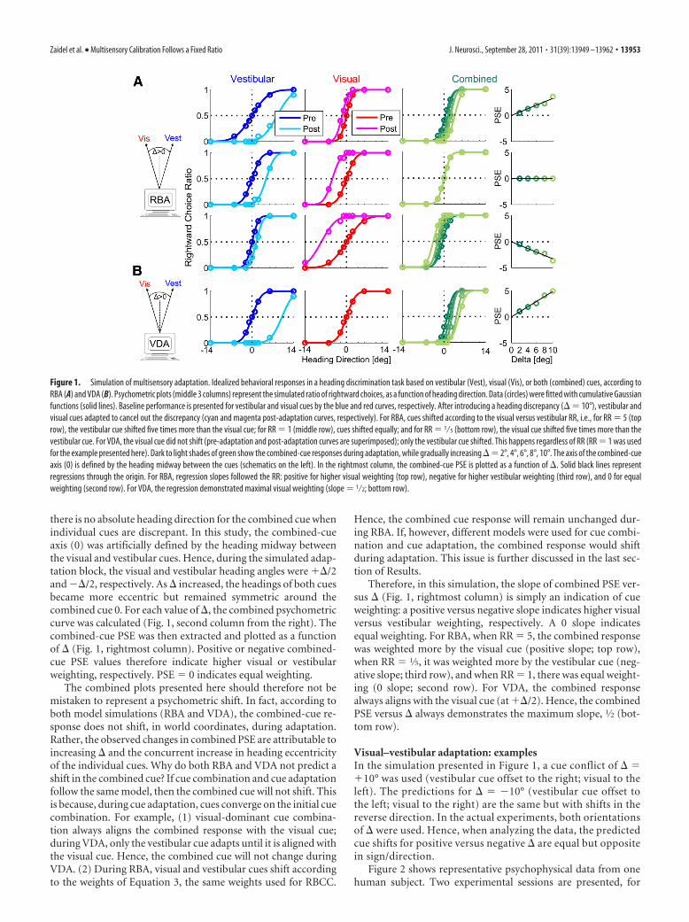
Cue adaptation magnitude does not correlate with relativecue reliabilityThe magnitude of individual-cue PSE shifts were plotted as a func-tion of RR (Fig. 5, leftmost column). Blue and red circles representvestibular and visual shifts, respectively; filled circles indicate signif-icant shifts. For both the human (Fig. 5A) and monkey (Fig. 5B)data, linear regressions were calculated separately for the visual andvestibular cues. Dependence of cue adaptation magnitude on RRwas assessed by testing whether the p value of Pearson’s correlationcoefficient was (0.05. Strikingly, there were no significant correla-tions between vestibular or visual PSE shifts versus RR: in the humandata, r # 0.16 (p # 0.11) and r # 0.11 (p # 0.29) for the vestibularand visual correlations, respectively. This is in contrast to the RBAprediction of a positive correlation for vestibular PSE shifts and anegative correlation for visual PSE shifts. In the monkey data, a smalltendency for opposite dependence was seen, but the slopes were notsignificantly different from 0; r#0.12 (p#0.23) and r#)0.13 (p#0.19) for the monkey vestibular and visual correlations, respectively.

The vestibular cue adapts more than the visual cue, regardlessof reliability ratioThe distributions of vestibular and visual PSE shifts (for all RRspooled) are presented by blue and red histograms in Figure 5 (mid-dle column), respectively. The filled sections in the bars representsignificant shifts. Cue shift distributions were analyzed statisticallyunder the null hypothesis of no shift, and p values were calculatedusing t tests and the Bonferroni’s correction for multiple compari-sons. The mean vestibular and visual shifts (blue and red dotted linessuperimposed on the histograms) were significantly positive, i.e., inthe “expected” direction, for both the human (Fig. 5A) and monkey(Fig. 5B) data (p ( 0.0001 for all four comparisons). Furthermore,the average vestibular shift was significantly greater than the average

Figure 3. Example of monkey multisensory adaptation. Two sessions from one monkey of visual–vestibular adaptation arepresented. For both sessions, visual coherence # 100% (RR ' 1). Plotting conventions are the same as Figures 1 and 2. Oppositevisual–vestibular heading discrepancies ($) were used for the two examples: in A, $ was positive. Hence, results can be compareddirectly with the simulation results of Figure 1 (which also used positive $). In B, $ was negative. Hence, shifts are expected in thereverse direction. Unlike Figures 1 and 2, there are no combined-cue data during the adaptation trials from the monkey experi-ment. R 2 $ 0.9 for all psychometric fits. Vis, Visual; Vest, vestibular.


visual shift, in both the human (p ( 0.01) and monkey (p ( 0.0001)data. The ratio of vestibular to visual PSE shift was "2:1 (1.75 forhumans and 2.30 for monkeys).

When grouping the data by low, medium, and high RR (right-most column), the mean vestibular PSE shift (blue) was alwaysgreater than the mean visual shift (red), even for low RR. This, too, isdemonstrated for both the human and monkey data and is contraryto the RBA prediction. Furthermore, comparing the mean PSE shiftfor low RR versus high RR (separately for visual and vestibular cues)revealed no significant differences for either the human or monkeydata (p ' 0.2 for all four comparisons, using a t test). However, wedid find that the SD for visual PSE shifts (red vertical lines) wassignificantly greater at low RR than high RR, for both the human andmonkey data (p ( 0.0001, using a +2 test and the Bonferroni’s cor-rection for multiple comparisons). In contrast, the SDs for vestibularPSE shifts (blue vertical lines) remained unchanged for both thehuman and monkey data (p ' 0.1). Hence, the only factor depen-dent on RR was visual PSE shift variability.

The finding that the vestibular cue shifts more and the visualcue less than expected by RBA is also demonstrated when analyz-ing proportional cue shifts. For this analysis, proportional PSEshifts were calculated as follows:

Proportional Visual PSE Shift %Visual PSE Shift

!Visual PSE Shift!* !Vestibular PSE Shift!

Proportional Vestibular PSE Shift %Vestibular PSE Shift

!Visual PSE Shift!* !Vestibular PSE Shift!

.

(6)

It should be noted that, when cues shift in the unexpected direc-tion, calculating the proportional PSE shift may be an ill-posedproblem.

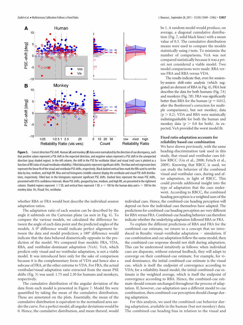
Expected proportional PSE shifts were predicted by the rela-tive cue reliabilities according to RBA. In Figure 6, the propor-tional shift data are plotted versus the expected proportionalshifts. Blue and red lines represent regressions for the vestibularand visual data, respectively, and shaded regions represent 95%confidence bands of the regressions based on 1000 bootstrappeddatasets. The diagonal (dashed) lines represent the expected re-gression if proportional shifts were to follow prediction. Signifi-cance was judged by whether or not the 95% confidence bandincluded the diagonal. In the human data (Fig. 6A), the relativevestibular shift was significantly greater than expected, and therelative visual shift was significantly less than expected. In themonkey data (Fig. 6B), the relative vestibular shift was greater(albeit not significantly) than expected, and the relative visualshift was significantly less than expected.

A model of fixed-ratio adaptation better accounts for visualand vestibular PSE shiftsOur findings that cue adaptation magnitude does not correlatewith relative cue reliability and that the vestibular cue adaptsmore than the visual cue, regardless of reliability ratio (Fig. 5),strongly implicate an FRA model. Furthermore, by dividing theaverage vestibular shift by the average visual shift, we found thatthe ratio representative of the FRA model was "2:1. However,cue adaptation-ratio analysis on a session-by-session basis, asdescribed by Burge et al. (2010) and in our comparable Figure 4,seemed to suggest that there might also be a reliability-basedcomponent. Hence, we performed additional analysis to see

Figure 4. Adaptation ratio. Population data are presented for both humans (A) and monkeys (B). Data in the left, middle, and right columns are sorted by low, medium, and high RR (ratio of visualto vestibular reliability), respectively. Each data point represents the adaptation observed in one experimental session, plotted as the shift in vestibular (Ves) PSE versus the shift in visual PSE. PSEshift was calculated as the difference between the pre-adaptation and post-adaptation PSEs. Error bars on the data points represent %1 SD of the PSE shift (calculated by bootstrapping thepsychometric curve data 2000 times). Squares and circles represent sessions with positive $ (vestibular to the right of visual) and negative $ (vice versa) discrepancies, respectively. The brown solidlines represent type II regressions of the data points, weighting each data point by its inverse (mean visual and vestibular) SD. The regression lines were constrained to pass through the origin. Thebrown shaded regions represent the 95% confidence bands of the regression lines (from 1000 bootstrapped datasets). Gray shading indicates regions where vestibular and visual cues shift in thesame direction (unexpected by internal consistency theory). Histograms (far right column) indicate that the sum of the absolute visual and vestibular shifts (across all RRs) were primarily (10°(vertical dashed line). n # 45, 38, 17 (100 total) for human low, medium, and high RR, respectively. n # 36, 28, 44 (108 total) for monkey low, medium, and high RR, respectively.


whether RBA or FRA would best describe the individual sessionadaptation ratios.

The adaptation ratio of each session can be described by theangle it subtends on the Cartesian plane (as seen in Fig. 4). Tocompare the various models, we calculated the difference be-tween the angle of each data point and the predicted angles of themodels. A 0° difference would indicate perfect alignment be-tween the data and model prediction; a 180° difference wouldindicate that the data behaved diametrically opposite to the pre-diction of the model. We compared four models: FRA, VDA,RBA, and vestibular-dominant adaptation (VeA). VeA, whichpredicts only visual and no vestibular adaptation, is not a viablemodel. It was introduced here only for the sake of comparisonbecause it is the complementary form of VDA and hence also asubcase of FRA, at the other extreme to VDA. For FRA, the actualvestibular/visual adaptation ratio extracted from the mean PSEshifts (Fig. 5) was used: 1.75 and 2.30 for humans and monkeys,respectively.

The cumulative distribution of the angular deviation of thedata from each model is presented in Figure 7. Model fits werequantified by taking the mean of the cumulative distribution.These are annotated on the plots. Essentially, the mean of thecumulative distribution is equivalent to the normalized area un-der the curve. For a perfect model, all angular deviations would be0. Hence, the cumulative distribution, and mean thereof, would

be 1. A random model would produce, onaverage, a diagonal cumulative distribu-tion (Fig. 7, solid black lines) with a meanvalue of 0.5. The cumulative distributionmeans were used to compare the modelsstatistically using t tests. To minimize thenumber of comparisons, VeA was notcompared statistically because it was a pri-ori not considered a viable model. Twomodel comparisons were made: RBA ver-sus FRA and RBA versus VDA.

The results indicate that, even for session-by-session shift-ratio analysis (which sug-gested an element of RBA in Fig. 4), FRA bestdescribes the data for both humans (Fig. 7A)and monkeys (Fig. 7B). FRA was significantlybetter than RBA for the human (p # 0.012,after the Bonferroni’s correction for multi-ple comparisons), but not monkey, data(p ' 0.2). VDA and RBA were statisticallyindistinguishable for both the human andmonkey data (p ' 0.8 for both). As ex-pected, VeA provided the worst model fit.

Fixed ratio adaptation accounts forreliability based cue combinationWe have shown previously, with the sameheading-discrimination task used in thisstudy, that visual and vestibular cues fol-low RBCC (Gu et al., 2008; Fetsch et al.,2009). Knowing that RBCC is used, wecan study the behavior of the combinedvisual and vestibular cues, during and af-ter adaptation, in light of RBCC. Thiscould provide additional insight into thetype of adaptation that the cues under-went. According to RBCC, the combinedheading perception is a weighted sum of the

individual cues. Hence, the combined-cue heading perception willdepend on how the individual cues themselves have adapted. Thepredictions for combined-cue heading perception are very differentfor RBA versus FRA. Combined-cue heading behavior can thereforeindicate whether the underlying adaptation followed RBA or FRA.

To explain the different predictions of RBA and FRA for thecombined-cue estimate, we return to a concept that we intro-duced in Results: visual–vestibular adaptation ) simulation. Ifcue combination and cue adaptation follow the same model, thenthe combined-cue response should not shift during adaptation.This can be understood intuitively as follows: when individualcues are disparate, without external feedback, they will adapt toconverge on their combined-cue estimate. For example, for vi-sual dominance, the initial combined-cue estimate is the visualcue, which is itself the endpoint of convergence according toVDA; for a reliability-based model, the initial combined-cue es-timate is the weighted average, which is itself the endpoint ofconvergence according to RBA. Hence, the combined-cue esti-mate should remain unchanged throughout the process of adap-tation. If, however, cue-adaptation uses a different model to cuecombination, then combined-cue perception should change dur-ing adaptation.

For this analysis, we used the combined-cue behavior dur-ing adaptation, available in the human (but not monkey) data.The combined-cue heading bias in relation to the visual and

Figure 5. Correct direction PSE shift. Human (A) and monkey (B) data were normalized by the direction of cue discrepancy, suchthat positive values represent a PSE shift in the expected direction, and negative values represent a PSE shift in the unexpecteddirection (gray shaded region). In the left column, the shift in the PSE for vestibular (blue) and visual (red) cues is plotted as afunction of RR (ratio of visual/vestibular reliability). Filled data points represent significant shifts. The blue and red regression linesrepresent the linear fit of the visual and vestibular PSE shifts, respectively. Black dashed vertical lines mark the RRs used to sort thedata by low, medium, and high RR. Blue and red histograms (middle column) display the vestibular and visual PSE shift distribu-tions, respectively. Filled bars in the histograms represent significant PSE shifts. Dashed lines represent the mean PSE shifts,presented with 95% confidence intervals. Mean PSE shifts, grouped by low, medium, and high RR, are presented in the rightmostcolumn. Shaded regions represent %1 SD, and vertical lines represent 1 SD. n # 100 for the human data and n # 108 for themonkey data. Vis, Visual; Ves, vestibular.


vestibular cues was extracted from the data by finding theslope of the combined-cue PSE versus $. As explained aboveand presented in Figures 1 and 2, the slope of the combined-cue PSE versus $ ranges from )1⁄2 to 1⁄2. A slope of 1⁄2 wouldindicate complete visual dominance, and a slope of )1⁄2 wouldindicate completed vestibular dominance. A slope of 0 would indi-cate equal weighting of visual and vestibular cues. RBCC couldtherefore be quantified by the slope of the combined-cue PSEversus $.

In Figure 8 A, we demonstrate, through simulation, the pre-dicted responses of the RBA and FRA models to an introducedheading discrepancy ($) between the cues. Like the simulationfor Figure 1, the visual cue was presented at )$/2 and thevestibular cue at &$/2. Pre-adaptation, combined-cue PSEslopes that would result from visual or vestibular cue domi-nance are represented by the red and blue solid lines, respec-tively, and the RBCC is represented by the dark green line (Fig.8 A; same for FRA and RBA). Pre-adaptation curves can beunderstood as follows: visual dominance would result in acombined-cue PSE versus $ slope of 1⁄2 (red line), and vestib-

ular dominance would result in a slope of )1⁄2, for RR '' 1,RBCC asymptotes to visual dominance, whereas for RR # "0,it asymptotes to vestibular dominance.

As we demonstrated above, internal consistency was notachieved in our data. Hence, we did not constrain the models tocomplete adaptation; rather the extent of adaptation was a pa-rameter that ranged from 0 (pre-adaptation) to 1 (internal con-sistency). In this simulation, an adaptation extent of 0.65 wasused. The vestibular/visual adaptation ratio used for the FRAsimulation was 1.75, because this was the actual ratio extractedfrom the data (Fig. 5A). After adaptation, cyan and magentalines represent the combined PSE slope that would result fromvisual and vestibular dominance, respectively. Similar to pre-adaptation, post-adaptation RBCC asymptotes to these curves.For RBA (Fig. 8A, left), the cues adapted according to the sameweights as RBCC. Hence, the RBCC remained unchanged evenafter adaptation (superimposed on the dark green curve). In con-trast, according to FRA, the cues adapted at a fixed ratio regard-less of RR (Fig. 8A, right). Because adaptation followed differentweights to cue combination, the RBCC response changed duringadaptation (light green curve).

For FRA, two major changes are evident in the RBCC curve:(1) the entire curve shifted vertically, as seen by the y-intercept,and (2) the curve narrowed, as seen by the reduced y-amplitude.

Figure 6. Actual versus expected proportional PSE shift. Actual versus expected proportionalPSE shifts are plotted for the human (A) and monkey (B) data. Blue and red lines represent typeII regressions of the vestibular and visual data (blue and red circles), respectively. The regressionlines were constrained to pass through the origin. Blue and red shaded regions represent 95%confidence bands of the regressions. If PSE shifts were to follow the RBA predictions, the regres-sion for both cues would lie on the line y # x (dashed black line). Gray shading representsregions where adaptation was in the unexpected direction. Vis, Visual; Ves, vestibular.

Figure 7. Adaptation data were best represented by a fixed-ratio model. When plotted onthe Cartesian plane, vestibular versus visual PSE adaptation can be described by a vector. Theangle of that vector represents the ratio of vestibular/visual adaptation. Here we compared theadaptation angles extracted from the data with those predicted from four different models:FRA, VDA, RBA, and VeA. The cumulative distribution of the difference between the actual andpredicted angles was plotted for both the human (A) and monkey (B) data. The black diagonalline represents the average cumulative distribution for random angles. The mean of the cumu-lative distribution is presented on the plots for each model.


The former resulted directly from the ratio of vestibular/visualadaptation, and the latter resulted directly from the extent ofadaptation. Hence, according to FRA, the combined-cue re-sponse can be predicted based on two model parameters: (1) theratio of vestibular/visual adaptation and (2) the extent of adapta-tion. These predictions are very different from RBA, which pre-dicts no change to cue combination during adaptation.

The actual RBCC data are presented in Figure 8B (circles).Data were fit by the following function:

f*RR+ % A !RR & 1

RR * 1* B, (7)

where RR is the visual/vestibular reliabil-ity ratio, and A and B are parameters usedfor optimization. A and B have a 1:1 rela-tionship with the extent and ratio of adap-tation as follows:

A %1 & extent

2

B %extent ! *ratio & 1+

2 ! *ratio * 1+.

(8)

Hence, each combination of the two pa-rameters (adaptation ratio and adaptationextent) represents a specific RBCC curve.The goodness of fit (R 2) was calculated foreach curve according to the standardformula:

R2 % 1 &residual sum of squares

total sum of squares.

(9)

Because the curves were defined externallyto span the parametric range (and not fittedto the data), some curves provided a worsefit than the data mean. For these curves,Equation 9 would result in a negative value.Hence, R2 was truncated at 0.

Figure 8C presents the R 2 values for allpossible combinations of adaptation ratioand adaptation extent. The optimal fit isrepresented by a dashed line in Figure 8Band a black dot in Figure 8C. According tothe FRA model, we should be able to pre-dict the RBCC fit based on the adaptationratio and adaptation extent. Although theadaptation extent may be unknown (thesedata are taken during the course of adap-tation), the adaptation ratio should followthe same ratio extracted from the cueshifts, presented above (Fig. 5). The actualadaptation ratio extracted from the data isrepresented by the solid white line in Fig-ure 8C (the dashed white line representsthe ratio from the monkey data). Fittingthe function according to the actual adap-tation ratio (with only one free parameter,adaptation extent) resulted in an RBCC fitalmost identical to the optimal fit. This ispresented by the light green curve in Fig-ure 8B and the light green dot in Figure

8C. In contrast, the RBA prediction was worse than the data mean.This can be seen by the dark blue region at the bottom of Figure 8C,because the RBA curve (which does not change during adaptation) isessentially identical to an FRA curve with adaptation extent of 0 (asseen in Fig. 8A). The very finding that the combined response un-dergoes adaptation indicates that cue combination and cue adapta-tion cannot be using the same model/weights. The finding that FRAcan account for RBCC provides additional support for the FRAmodel.

Finally, the deviance of the actual combined-cue PSE values(as a function of $) from the FRA and RBA predictions ispresented in Figure 8 D. The actual combined-cue PSE values

Figure 8. Fixed-ratio adaptation accounts for reliability-based cue combination. A, We present a simulation of theexpected RBCC adaptation. RBCC was quantified by the slope of the combined-cue PSE versus $ (as presented in Figs. 1, 2).Two models of adaptation were simulated: RBA (left plot) and FRA (right plot). For FRA, a vestibular/visual adaptation ratioof 1.75 was used (as extracted from the actual cue shifts). For both simulations, partial (65%) adaptation is presented, i.e.,the cues did not reach internal consistency. Before adaptation, combined-cue PSE slopes that would result from visual orvestibular cue dominance are represented by the red and blue horizontal lines, respectively, and post-adaptation bymagenta and cyan curves, respectively. RBCC is represented by the dark green and light green curves, before and afteradaptation, respectively. For RBA, RBCC remained unchanged (pre-adaptation and post-adaptation curves are superim-posed). For FRA, the RBCC curve amplitude changed, and its y-cut became non-0. B, The actual data of combined-cue PSEversus $ slopes is presented (circles). Two outliers are marked by & symbols. The optimal FRA model fit is represented bythe black dashed curve, and the model fit with adaptation ratio constrained at 1.75 is presented by the light green curve.C, The R 2 values of the FRA model fit for all possible parameters of adaptation ratio and extent are presented. The lightgreen and (partially hidden) black dots represent the R 2 values for the ratio-constrained and optimal fits, respectively. Thewhite vertical lines represent the adaptation-ratio extracted from the human (solid) and monkey (dashed) data. D, Theaverage difference between the actual combined PSEs and the predictions of the models are presented. Dark and lightgreen lines show the deviances for RBA and FRA, respectively. Error bars represent the SEM. vis, Visual; ves, vestibular.


were closer to the initial (pre-adaptation) visual cue for low RR andinitial vestibular cue for high RR thanpredicted by RBA (dark green lines).These data indicate that the visual andvestibular cues did not shift according toRBA. In contrast, FRA adaptation predic-tions, using the parameters from Figure 8,were indistinguishable from the actualcombined-cue PSE values, for all RR (lightgreen curves).

DiscussionIn this study, we probed the nature of mul-tisensory cue calibration in the absence ofexternal feedback. We found that, given aheading-direction discrepancy betweenvisual and vestibular cues, both cues un-derwent mutual adaptation toward oneanother. Quantitatively, the extent of in-dividual cue adaptation followed a fixedratio, regardless of relative cue reliability.Specifically, the ratio of vestibular/visualadaptation was "2:1 for both humans andmonkeys. This finding is particularly strik-ing because, during cue integration, visualand vestibular cues are weighted accordingto their relative reliabilities (Gu et al., 2008;Fetsch et al., 2009; Butler et al., 2010). Ourresults therefore indicate that multisensorycue integration and cue calibration followdifferent mechanisms/principles: cue inte-gration is reliability based, whereas cue calibration follows a fixedratio.

Reliability-based cue integration has been demonstrated in anumber of multisensory paradigms (Jacobs, 1999; van Beers et al.,1999, 2002; Landy and Kojima, 2001; Ernst and Banks, 2002; Gep-shtein and Banks, 2003; Knill and Saunders, 2003; Alais and Burr,2004; Jurgens and Becker, 2006; Gu et al., 2008; Fetsch et al., 2009;Butler et al., 2010). However, quantitative testing of the nature ofmultisensory cue calibration is lagging. Burge et al. (2010) recentlypioneered a paradigm to quantitatively test the reliability-basedmodel for visual–haptic calibration. They reported that visual–hap-tic cues follow a model of reliability-based adaptation. In our study,we emulated their paradigm but with visual–vestibular calibration.When using similar methods of analysis, also our data suggested aninfluence of relative reliability on cue adaptation. However, addi-tional analysis revealed that visual–vestibular calibration is muchbetter accounted for by a model of fixed-ratio adaptation thanreliability-based adaptation.

To explain why analyzing the data according to the previousmethods (Fig. 4) could suggest reliability-based adaptation evenif adaptation was not reliability based, we present a simulation inFigure 9: Each subplot displays a simulated probability densityfunction corresponding to the subplots of Figure 4. The proba-bility density functions were plotted by color scale, in which redrepresents high probabilities and blue represents low probabili-ties. All probability density functions were generated as the com-bination of two bivariate Gaussians: “two,” one for positive andone for negative $; and “bivariate,” for visual and vestibularshifts. The Gaussian means for visual and vestibular shifts werethe same across all plots: ()1°, 1°) for positive $ and (1°, )1°) fornegative $. Because the means were of equal magnitude and the

same for all RRs, the simulated probability density functions didnot represent reliability-based adaptation.

The Gaussian variances were taken from the actual data (thesame variances were used for positive and negative $ Gaussians).As we described previously (Fig. 6, right column), vestibular PSEshift variability was unchanged across RRs, whereas visual PSEshift variability was strongly dependent on RR. (In itself, thisresult is not surprising because RR was controlled in the experi-ment by manipulating visual motion coherence only.) Therefore,for the Gaussians, we used the overall vestibular PSE shift vari-ance for all RRs and specific visual PSE shift variances for low,medium, and high RR. Hence, the only difference between theRRs (columns in Fig. 9) was the variability of visual PSE shifts.

A type II regression line of 2000 data points, generated fromeach probability density function in Figure 9, is displayed inwhite. The regression lines are strikingly similar to those of theactual data (Fig. 4). They, too, approach the horizontal for low RRand vertical for high RR. However, their differences in orienta-tion exist exclusively because of visual PSE shift variance, becausethere were no other differences between the simulations. Hence,changes in variability alone can cause changes in the orientationof the regression lines, similar to those seen in the data. Therefore,regression line orientation may not accurately represent the ratioof cue adaptation. Visual inspection of the data by Burge et al.(2010) seems to indicate that there, too, visual PSE shift variabil-ity could change with RR. Hence, additional analysis may berequired to verify the model of adaptation.

The analyses in our paper strongly argue that visual–vestibularcalibration follows fixed-ratio and not reliability-based adapta-tion. Particularly, we found that neither visual nor vestibularadaption correlated with RR. Rather, cue shifts remained con-

Figure 9. Simulated effects of visual PSE shift variability. Each subplot presents a simulated probability density function (PDF)corresponding to the subplots in Figure 4. Left, middle, and right columns represent low, medium, and high RRs, respectively. AllPDFs were generated from two bivariate Gaussians: one with mean (1°, )1°) and the other with mean ()1°,1°). Gaussianvariances were set according to the actual PSE shift variances extracted from the human and monkey data (A and B, respectively).Vestibular PSE shift variance was set according to the overall variance and did not change for different RRs: 2.4° for the human dataand 7.0° for the monkey data. Visual PSE shift variance was set individually for low medium and high RR: 15.0°, 2.3°, and 1.2°,respectively, for the human data; and 9.0°, 3.4°, and 0.8°, respectively, for the monkey data. A type II regression line of 2000 datapoints, generated from each PDF, is displayed in white. The regression lines were constrained to pass through the origin. Ves,Vestibular.


stant regardless of whether the visual or the vestibular cue wasmore reliable, indicating that cue calibration does not follow thesame mechanism as cue integration. The fact that our findingswere consistent for both humans and monkeys consolidates theseresults. Even the vestibular/visual shift ratio ("2:1) was similarfor humans and monkeys. Finally, only through modeling fixed-ratio adaptation (using the ratio extracted from the data) were wewere able to account for reliability-based cue integration duringthe adaptation process.

Ernst and Di Luca (2011) suggest that using relative cuereliability for multisensory calibration may be a suboptimalstrategy because variance of a cue does not necessarily deter-mine the probability of it being biased. This brings us back tothe difference between reliability and accuracy: reliability isthe inverse variance of the probability distribution that de-scribes the contribution of a sensory signal to the perceptualestimation. In contrast, accuracy is the probability that the sen-sory signal truly represents the real-world physical property. Ac-curacy and reliability are therefore different properties. Hence,relative cue reliability may not be a good indication as to whichcue most likely requires calibration.

If the goal of multisensory cue integration is optimal percep-tion (in the sense of improving precision), a reliability-basedmodel makes sense. In contrast, assuming that the goal of cuecalibration is improvement of cue accuracy, an accuracy-basedmechanism would seem more appropriate. The estimate of cueaccuracy of the brain probably has a much longer time constantthan that of cue reliability. Accordingly, it is possible that ourfinding of fixed-ratio adaptation is only relatively fixed, but achange in cue accuracy could change the rate of adaptation. Ourfinding of higher vestibular versus visual adaptation suggests thatthe visual cue is more accurate than the vestibular cue in headingdiscrimination. In this study, we manipulated cue reliability;however, we did not manipulate cue accuracy. To test the hy-pothesis that cue calibration follows relative accuracy, cue accu-racy would need to be manipulated.

The proposal that cue accuracy is more important than cuereliability for multisensory calibration is in line with Gori et al.(2008, 2010) who found that, during development, children donot integrate visual and haptic cues optimally, but rather, touchdominates discrimination of size, and vision dominates discrim-ination of orientation, even in conditions in which the dominantsense is far less precise than the other. They propose that thesensory dominance may reflect cross-modal calibration, in whichthe more accurate sense calibrates the other (Burr and Gori,2011).

Visual dominance has been a prevalent theory (Rock and Victor,1964; Brainard and Knudsen, 1993). Hence, it has been used as astandard by which to compare reliability-based models (van Beers etal., 2002; Burge et al., 2010). However, visual-dominant adapta-tion does not represent the general reliability-independentalternative. In fact, it is only a specific subcase of fixed-ratioadaptation (in which the ratio of non-visual/visual adaptationtends to infinity). In this study, we present fixed-ratio adap-tation as a novel, yet simple, model and recommend using it asa reliability-independent standard by which to comparereliability-based models. Our finding that visual–vestibularcalibration actually follows the fixed-ratio adaptation modelclearly highlights its relevance.

In conclusion, our results indicate that visual–vestibularcue calibration does not follow the same mechanism as cueintegration. Cue integration is reliability based, whereas cuecalibration follows a fixed ratio. It is possible that fixed-ratio

adaptation may be only relatively fixed and that the ratio ofadaptation may change with cue accuracy. To test this, multi-sensory cue adaptation needs to be tested as a function ofrelative cue accuracy.

ReferencesAlais D, Burr D (2004) The ventriloquist effect results from near-optimal

bimodal integration. Curr Biol 14:257–262.Atkins JE, Jacobs RA, Knill DC (2003) Experience-dependent visual cue

recalibration based on discrepancies between visual and haptic percepts.Vision Res 43:2603–2613.

Brainard MS, Knudsen EI (1993) Experience-dependent plasticity in the in-ferior colliculus: a site for visual calibration of the neural representation ofauditory space in the barn owl. J Neurosci 13:4589 – 4608.

Burge J, Girshick AR, Banks MS (2010) Visual-haptic adaptation is deter-mined by relative reliability. J Neurosci 30:7714 –7721.

Burr D, Gori M (2011) Multisensory integration develops late in humans.In: The neural bases of multisensory processes (Murray MM, WallaceMT, eds), pp 345–362. Boca Raton: CRC.

Butler JS, Smith ST, Campos JL, Bulthoff HH (2010) Bayesian integration ofvisual and vestibular signals for heading. J Vis 10:23.

Ernst MO, Banks MS (2002) Humans integrate visual and haptic informa-tion in a statistically optimal fashion. Nature 415:429 – 433.

Ernst MO, Di Luca M (2011) Multisensory perception: from integration toremapping. In: Sensory cue integration (Trommershauser J, Kording K,Landy MS, eds), pp 224 –250. New York: Oxford UP.

Fetsch CR, Turner AH, DeAngelis GC, Angelaki DE (2009) Dynamic re-weighting of visual and vestibular cues during self-motion perception.J Neurosci 29:15601–15612.

Gepshtein S, Banks MS (2003) Viewing geometry determines how visionand haptics combine in size perception. Curr Biol 13:483– 488.

Ghahramani Z, Wolpert DM, Jordan MI (1997) Computational models ofsensorimotor integration. In: Self-organization, computational maps andmotor control (Morasso PG, Sanguineti V, eds), pp 117–147. Amsterdam:Elsevier.

Gori M, Del Viva M, Sandini G, Burr DC (2008) Young children do notintegrate visual and haptic form information. Curr Biol 18:694 – 698.

Gori M, Sandini G, Martinoli C, Burr D (2010) Poor haptic orientationdiscrimination in nonsighted children may reflect disruption of cross-sensory calibration. Curr Biol 20:223–225.

Gu Y, DeAngelis GC, Angelaki DE (2007) A functional link between areaMSTd and heading perception based on vestibular signals. Nat Neurosci10:1038 –1047.

Gu Y, Angelaki DE, Deangelis GC (2008) Neural correlates of multisensorycue integration in macaque MSTd. Nat Neurosci 11:1201–1210.

Gu Y, Fetsch CR, Adeyemo B, Deangelis GC, Angelaki DE (2010) Decodingof MSTd population activity accounts for variations in the precision ofheading perception. Neuron 66:596 – 609.

Guedry FE (1974) Psychophysics of vestibular sensation. In: The vestibularsystem (Kornhuber HH, ed), pp 1–154. New York: Springer.

Jacobs RA (1999) Optimal integration of texture and motion cues to depth.Vision Res 39:3621–3629.

Judge SJ, Richmond BJ, Chu FC (1980) Implantation of magnetic searchcoils for measurement of eye position: an improved method. Vision Res20:535–538.

Jurgens R, Becker W (2006) Perception of angular displacement withoutlandmarks: evidence for Bayesian fusion of vestibular, optokinetic,podokinesthetic, and cognitive information. Exp Brain Res174:528 –543.

Knill DC, Pouget A (2004) The Bayesian brain: the role of uncertainty inneural coding and computation. Trends Neurosci 27:712–719.

Knill DC, Saunders JA (2003) Do humans optimally integrate stereo andtexture information for judgments of surface slant? Vision Res43:2539 –2558.

Knudsen EI (2002) Instructed learning in the auditory localization pathwayof the barn owl. Nature 417:322–328.

Landy MS, Kojima H (2001) Ideal cue combination for localizing texture-defined edges. J Opt Soc Am A Opt Image Sci Vis 18:2307–2320.

Lewald J (2002) Rapid adaptation to auditory-visual spatial disparity. LearnMem 9:268 –278.

MacNeilage PR, Banks MS, DeAngelis GC, Angelaki DE (2010) Vestibular


heading discrimination and sensitivity to linear acceleration in head andworld coordinates. J Neurosci 30:9084 –9094.

Ohmi M (1996) Egocentric perception through interaction among manysensory systems. Brain Res Cogn Brain Res 5:87–96.

Rock I, Victor J (1964) Vision and touch: an experimentally created conflictbetween the two senses. Science 143:594 –596.

Scarfe P, Hibbard PB (2011) Statistically optimal integration of biased sen-sory estimates. J Vis 11:pii:12.

Spence C (2009) Explaining the Colavita visual dominance effect. ProgBrain Res 176:245–258.

van Beers RJ, Sittig AC, Gon JJ (1999) Integration of proprioceptive andvisual position-information: An experimentally supported model. J Neu-rophysiol 81:1355–1364.

van Beers RJ, Wolpert DM, Haggard P (2002) When feeling is more impor-tant than seeing in sensorimotor adaptation. Curr Biol 12:834 – 837.

Warren WH, Hannon DJ (1988) Direction of self-motion is perceived fromoptical-flow. Nature 336:162–163.

Watt SJ, Akeley K, Ernst MO, Banks MS (2005) Focus cues affect perceiveddepth. J Vis 5:834 – 862.

Wichmann FA, Hill NJ (2001a) The psychometric function. I. Fitting, sam-pling, and goodness of fit. Percept Psychophys 63:1293–1313.

Wichmann FA, Hill NJ (2001b) The psychometric function. II. Bootstrap-based confidence intervals and sampling. Percept Psychophys 63:1314 –1329.

Witten IB, Knudsen EI (2005) Why seeing is believing: merging auditoryand visual worlds. Neuron 48:489 – 496.

Yuille AL, Bulthoff HH (1996) Bayesian decision theory and psychophysics.In: Perception as Bayesian inference (Knill DC, Richards W, eds). NewYork: Cambridge UP.


behavioral/systems/cognitive ...nba.uth.tmc.edu/homepage/cnjclub/2011...

Documents