This paper presents preliminary findings and is being distributed to economists

and other interested readers solely to stimulate discussion and elicit comments.

The views expressed in this paper are those of the author and are not necessarily

reflective of views at the Federal Reserve Bank of New York or the Federal

Reserve System. Any errors or omissions are the responsibility of the author.

Federal Reserve Bank of New York

Staff Reports

Banking across Borders

Friederike Niepmann

Staff Report No. 576

October 2012

Revised October 2013

Banking across Borders

Friederike Niepmann

Federal Reserve Bank of New York Staff Reports, no. 576

October 2012; revised October 2013

JEL classification: F21, F23, F34, G21

Abstract

The international linkages between banks play a crucial role in today’s global economy. Existing

models explain these links on the basis of portfolio theory, in which banks diversify lending.

These models have found only limited empirical support and do not speak to many relevant

dimensions of the data. For example, they do not address heterogeneity in the degree to which

banking sectors fund their foreign operations locally in foreign markets. This paper proposes an

alternative theory to explain banking across borders that is based on elements of international

trade theory. In the model, banking across borders arises because countries differ in their relative

factor endowments and in the efficiency of their banking sectors. Based on these differences, the

pattern of foreign bank asset and liability holdings emerges endogenously. This parsimonious

model provides a rationale for different dimensions of heterogeneity in foreign bank activities and

clarifies the interpretation of international banking data. Its predictions are consistent with

observed patterns in the data.

Key words: cross-border banking, international capital flows, trade in banking services

_________________

Niepmann: Federal Reserve Bank of New York (e-mail: friederike.niepmann@ny.frb.org). The

author is grateful to Andrew Bernard, Giancarlo Corsetti, and Russell Cooper for constant advice

and encouragement. Special thanks go to Iman van Lelyveld, De Nederlandsche Bank (DNB),

and Deutsche Bundesbank. Part of this paper was written while the author was an intern at DNB

and a visiting researcher at Deutsche Bundesbank. For their helpful comments, the author also

thanks Pol Antras, Elena Carletti, Francesco Caselli, Simon Gilchrist, Beata Javorcik, Philip

Lane, Peter Neary, Emanuel Ornelas, Romain Ranciere, Katheryn Russ, Tim Schmidt-Eisenlohr,

Eberhard Schnebel, Daniel Sturm, and Silvana Tenreyro, as well as participants in the CESifo

Global Economy Area Conference 2012 and in the IMT session at the NBER Summer Institute

2013, in workshops and seminars at the University of Oxford, the University of Cambridge,

Trinity College Dublin, De Nederlandsche Bank, the London School of Economics, and the

European University Institute. The author also thanks the Bank for International Settlements and

Neeltje van Horen for making available some of the data used in this research, and Richard Peck

for excellent research assistance. An earlier version of this paper won the Distinguished CESifo

Affiliate Award 2012. The views expressed in this paper are those of the author and do not

necessarily reflect the position of the Federal Reserve Bank of New York or the Federal Reserve

System.

1 Introduction

The financial crisis in 2008/2009 highlighted the pivotal role of international financial linkages

between banks in the global economy.1 Research in the cross-border banking literature predom-

inantly relies on portfolio theory to explain these links.2 Portfolio models assume that financial

intermediaries invest abroad in order to diversify lending. There is, however, little empirical

support for diversification in the data. Aviat and Coeurdacier (2007) have found that banks

invest more in countries that show a stronger positive correlation with domestic returns, a

finding known as the “correlation puzzle”. In addition, portfolio frameworks do not provide a

rationale for the foreign liability holdings of banks and for the decisions of banks to operate

cross-border or through foreign affiliates. Accordingly, these models cannot address three rele-

vant dimensions of heterogeneity in the data. First, the extent to which banks operate through

foreign affiliates varies substantially across banking sectors. Second, banking sectors differ in

their foreign liability-asset gaps, a measure which has been related to the (in)stability of foreign

bank operations. Third, there is considerable heterogeneity in foreign bank participation across

countries, that is, foreign banks are differentially important in different countries.3

This paper uses elements of international trade theory to propose an alternative conceptual

framework explaining why and how international bank linkages are created. In the model,

countries differ in their returns to capital as well as in the efficiencies of their banking sectors.4

These differences generate banking across borders through two mechanisms. First, banks chan-

1Bank linkages matter for financial contagion and the transmission of macro shocks, for example. See, e.g.,Kaminsky and Reinhart (2000), Cetorelli and Goldberg (2011), Kalemli-Ozcan, Papaioannou and Perri (2013)and Cetorelli and Goldberg (forthcoming).

2Exceptions are de Blas and Russ (2012), Ennis (2001), and Eaton (1994). These papers are discussed aspart of the literature review in more detail.

3Recent work by Bruno and Shin (2012) explains cyclical fluctuations in cross-border bank flows but doesnot address these aspects either.

4The model combines Heckscher-Ohlin differences in factor endowments with technological differences in thespirit of Ricardo. While it borrows these elements from the international trade literature, the model does notfollow from relabeling existing theory.

1

nel capital to capital-scarce countries. At the same time, the more efficient banking sector

expands, whereas the less efficient banking sector contracts. Thus a cross-country pattern of

bank foreign asset and liability holdings emerges endogenously.

This parsimonious model makes progress in several dimensions. First of all, it delivers a

tractable theory of trade in banking services that endogenously pins down the cross-country

exposures of banking sectors on both the asset and the liability side of banks’ balance sheets.5

The empirical part of the paper shows that the key cross-sectional implications of the theory

are consistent with the conditional correlations in the data.

The paper provides a framework to explain the three dimensions of heterogeneity, which

have only been discussed from an empirical point of view: heterogeneity in the extent to which

banks operate through foreign affiliates, heterogeneity in liability-asset gaps, and heterogeneity

in foreign bank participation. The first type of heterogeneity is related to research by Mc-

Cauley, Ruud and Wooldridge (2002) and McCauley, McGuire and von Peter (2012).6 These

researchers at the Bank for International Settlements (BIS) observe that different banking

sectors follow different funding models, funding themselves to varying degrees globally or in-

ternationally. Global banking implies that banks raise funding abroad through foreign affiliates

(FDI) and invest the capital in the same foreign market. International banking denotes the

case in which a banking sector extends cross-border loans to foreign firms funded by domestic

deposits (arms-length export). The model is able to generate these activities and to show under

which conditions a banking sector engages in each of the two. The model also shows that a

third activity has to be distinguished. Banks may also conduct foreign sourcing, which I define

as raising funding abroad for investment at home.

5This paper also adds to the growing literature on services trade. See Francois and Hoekman (2010) for areview of recent developments in services trade research.

6See also McCauley, McGuire and von Peter (2010).

2

By defining and distinguishing different types of banking across borders, this paper also

provides guidance on how to interpret international banking data. Knowledge of cross-border

banking is largely based on reports of foreign positions gathered by the Bank for International

Settlements or on bank-level equivalents, which national central banks collect. These statistics

are complex. The model shows that consolidated banking statistics will always include inter-

national banking, global banking as well as foreign sourcing. In this regard, this paper helps

clarify some confusion around when to use locational or consolidated statistics. For example,

a gravity equation, where asset holdings increase one to one with the GDP of the source and

the destination country should not always hold.7

In the model, banks provide intermediation services, channeling capital from depositors

to firms at a cost that reflects banking sector efficiency in the economy. Entrepreneurs who

borrow from intermediaries have to pay this cost plus the interest rate paid out to depositors.

The interest rate is endogenously determined by the capital-labor ratio and banking sector

efficiency in the economy. In the open economy, entrepreneurs have the option to borrow

both from domestic and foreign banks. Banks in turn can raise deposits at home and abroad.

Countries differ in relative factor endowments and banking sector efficiencies so that autarky

interest rates and intermediation fees differ across countries.8

The model incorporates three additional elements. First, an entrepreneur who is served by

a foreign bank has to pay a cost τ proportionate to the loan he takes. The lower τ is, the more

freely capital can flow across borders: that is, the higher the degree of capital account openness.

Second, if banks raise capital abroad, they incur cost t, which reflects the degree of banking

sector liberalization. The lower the cost, the lower the barriers are to establishing a physical

7Aviat and Coeurdacier (2007) test predictions of a portfolio model based on the consolidated statistics,assuming that a one-to-one relationship between asset holdings and country sizes holds.

8This approach is similar to Ju and Wei (2010).

3

presence abroad. This interpretation implies that banks can extend loans cross-border/from

home but can only raise deposits through foreign affiliates abroad. Finally, it is assumed that

the more capital banks intermediate, the more capacity constrained and the less efficient they

become.

Taking the additional cost of being served by a foreign bank into account, entrepreneurs

minimize the cost of external funding, choosing the bank that offers the best combination of

interest rate and service fee. When differences in efficiencies and endowments are large across

countries relative to the transaction costs, trade in banking services occurs. In equilibrium,

banking sectors invest and borrow across borders so that gross returns to capital and service

fees are equilibrated.

The model shows under which conditions the three types of banking across borders occur. If

differences in returns are large, while there are no differences in efficiencies, the banking sector

of the capital abundant country engages in international banking, investing domestic capital

abroad. As a consequence it holds foreign assets but no foreign liabilities. If differences in

banking sector efficiencies are large, but endowments are similar, the more efficient banking

sector engages in global banking, raising capital abroad and investing this capital in the foreign

market. In this case the banking sector holds both foreign assets and foreign liabilities. If a

capital scarce country hosts a very efficient banking sector, its banks conduct foreign sourcing,

raising capital abroad for investment at home. Accordingly, they hold foreign liabilities but

no foreign assets on their balance sheets. These three special cases illustrate how the model

endogenously determines the cross-country foreign exposures of banking sectors. In general,

banking sectors engage in two of the three activities simultaneously.

Beyond rationalizing participation in global banking, international banking and foreign

4

sourcing, the model can also explain two other dimensions of heterogeneity across countries:

foreign liability-asset gaps and the degree of foreign bank participation. An extension shows

that the predictions of the model are robust to allowing for interbank lending, which yields

additional testable implications.

Using bank-level data from Deutsche Bundesbank and aggregated data from the Bank for

International Settlements, I find that the model is consistent with key conditional correlations

in the data. Conditional on country size and frictions, foreign asset and liability holdings of

the source banking sector are higher when the efficiency advantage of the source relative to

the destination country is larger. In addition, the ratio of foreign liabilities to foreign assets is

negatively correlated with capital abundance in the source country. To test for diversification,

I also include a measure of GDP growth correlations between countries in the regressions.

There is tentative evidence that banks diversify their assets. When differences in endowments,

differences in efficiencies, and bilateral FDI are controlled for, the diversification coefficient is

negative suggesting that banks invest more in countries with less synchronized business cycles.

The model provides a framework for thinking about banking across borders that is consistent

with key aspects of the data. Because it is simple but generates a rich structure, it can serve

as a basis for future research and can be used to develop theory that incorporates additional

features of the data, such as imperfect competition, bank heterogeneity and diversification.

In addition to contributing to the literature on cross-border banking, the analysis also relates

to the literature on international capital flows and financial frictions, highlighting two particular

aspects.9 First, the transaction costs banks face matter for equilibrium bank flows and for the

allocation of capital across countries. Second, the relationship between openness as well as

financial development of a country and capital flows is, in general, not linear. When a capital

9See, for example, Mendoza, Quadrini and Rıos-Rull (2009) and Antras and Caballero (2009).

5

scarce country liberalizes its banking sector and domestic banks become more efficient, it can

experience a capital outflow. This result depends on the market structure and the nature of

the transaction costs banks face, micro-level aspects which deserve more consideration in future

research.

More related literature Most papers in the cross-border banking literature either rely

conceptually on portfolio theory to explain banks’ international linkages (Walter (1981), Buch,

Koch and Koetter (2009), Bruno and Shin (2012)) or the structure of foreign bank operations is

exogenous. (for example, Dell’Ariccia and Marquez (2010), Niepmann and Schmidt-Eisenlohr

(forthcoming)). There are works that discuss different internationalization strategies of banks

(see Aliber (1984), Grubel (1989), Williams (1997), Berger (2007)) but only a few papers,

in addition to this paper, propose alternative theoretical models that do not build on asset

diversification to explain cross-border banking.

In de Blas and Russ (2012), a study of the impact of financial integration on loan pricing,

firms send out loan applications randomly to a limited number of banks, also applying at

foreign banks to minimize expected costs. In de Blas and Russ (2010), an earlier version,

firms love variety in loans so that banks offer differentiated products just as manufacturing

firms. Ennis (2001) assumes that information problems are reduced when banks operate across

regions. In Eaton (1994), financial centers emerge because authorities differ in their preferences

for protecting debtors as opposed to creditors and in their need for seignorage revenues. It is

the only work that provides an explicit theory to predict the geography of where financial firms

invest and raise funds.

The empirical literature on cross-border banking is more extensive than the theoretical

contributions. Exploring the omitted effects of differences in endowments and differences in

6

banking sector efficiencies between countries on banks’ foreign positions, this paper confirms

earlier empirical findings that institutions matter (see Papaioannou (2009)) and that banks

invest more in foreign countries that have higher GDP, fewer capital controls, and lower bank

entry barriers and that are closer in distance and culture (see, e.g., Buch (2003); Buch (2005);

Focarelli and Pozzolo (2005); Buch and Lipponer (2007); Claessens and Van Horen (2008)).10

Bank-to-bank versus direct lending has not been investigated.

The paper is organized as follows: section 2 presents background facts, section 3 introduces

the closed economy setup, section 4 studies the open economy, section 5 discusses empirical

evidence, and section 6 concludes.

2 Background Facts

2.1 Aggregate facts

Banks’ foreign activities are large and have been growing over time. Figure 1 shows the evolution

of the aggregate foreign asset holdings of 25 BIS reporting countries. The increase in foreign

assets after 1998 has been substantial both as a fraction of world GDP and compared to the

increase in international trade during the same period.11 A closer look at the data reveals that

they increased to a similar extent in destination countries of every income group.

The largest part of foreign assets is held in the non-bank private sector. In 2009, the 25

reporting countries had on average 55 percent of their foreign assets in a given destination

country invested in the private sector. 29 percent of foreign claims reflected assets vis-a-vis

other banks and around 16 percent vis-a-vis the public sector. This sectoral split has remained

10See, e.g., Goldberg (2007) and Cull and Martinez Peria (2010) for a review of the empirical literature.11See Committee on the Global Financial System (2010b).

7

largely stable over time.12 Data from Deutsche Bundesbank with information on German banks

in the year 2005 also provide statistics on the sectoral split of liabilities. For German banks,

borrowing from foreign banks is more important than borrowing from foreign depositors: the

share of bank liabilities was 61 percent in 2005 compared to non-bank-private liabilities that

accounted for 29 percent of total foreign liabilities.13

2.2 Heterogeneity across countries

The foreign activities of banking sectors differ considerably in several respects. In the following,

I review three dimensions of heterogeneity that have been discussed in the literature.

Global versus international One dimension of heterogeneity is the extent to which banking

sectors engage in international and global banking. Researchers at BIS have distinguished

between an international and a global funding model. In international banking, a bank raises

capital in its domestic market and lends it to a foreign market. In global banking, in contrast, a

bank obtains funds through foreign affiliates in a foreign market and intermediates them locally.

There is heterogeneity in the extent to which banking sectors follow the global or the

international model, which is illustrated in figure 2. It shows the ratio of foreign assets that

are held on the balance sheets of affiliates located in the respective destination country in

total foreign assets. In terms of the language of the BIS statistics, it displays the share of

local assets in foreign assets in the year 2009 of different banking sectors.14 While Spanish

banks operate mainly through foreign affiliates (more than 65 percent of all assets are held

by foreign affiliates), German banks conduct international business predominantly from home;

12The share of assets invested in the non-bank private sector tends to be higher in lower income countriescompared to high income countries.

13For a description of the data from BIS and Deutsche Bundesbank, see section 5.14The data that underly figures 2 and 3 were kindly provided by the Bank for International Settlements.

8

more than 80 percent of their foreign assets are held by banks located in Germany. This

difference suggests that Spanish banks engage more in global banking, while German banks do

more international banking. McCauley, Ruud and Wooldridge (2002) and McCauley, McGuire

and von Peter (2012) point out that banking sectors, in general, have been following increasingly

the global model rather than the international model, a phenomenon they call the “globalisation

of international banking”.

Liability-asset gaps A related dimension of heterogeneity is the heterogeneity in foreign

liability-asset gaps across banking sectors that capture how much of the foreign activities of

banks are funded through liabilities in the same country. Differences in liability-asset gaps

have been related to the stability of foreign bank operations. Researchers have indicated that

lending that is funded locally was more stable during the recent financial crisis (see Herrero and

Martinez Peria (2007), Cetorelli and Goldberg (2011), and de Haas and van Lelyveld (2011))

and that the related rollover risk is lower (see Cerutti (2013)). Under a pure global funding

model, the liability-asset gap of a banking sector should be 1. Under an international funding

model, it should be 0. Figure 3 shows that the ratio of assets to liabilities varies considerably

across banking sectors. Figures 2 and 3 together highlight that liability-asset gaps and the

degree to which banking sectors operate through foreign affiliates are correlated.

Foreign bank participation Heterogeneity can also be analyzed from the point of view

of a destination country. Claessens and van Horen (2012) study variation in foreign bank

participation across countries, which is measured as the share of lending by foreign banks

in total lending in a given country. Figure 4 displays the varying degrees of foreign bank

participation in the year 2009.15 While foreign banks do not play a major role in advanced

15The figure is based on data from Claessens and van Horen (2012), which was kindly provided by the authors.

9

countries, they are pivotal in Emerging Europe, especially, and also in many African and Latin

American countries. In Estonia, Jamaica and Zimbabwe, for example, more than 95 percent of

the domestic lending is done by foreign banks.

The three dimensions of heterogeneity have been studied in the aforementioned works with-

out relying on an explicit theoretical model and more or less in isolation. This paper presents

a model that can jointly explain them.

3 The Closed Economy Model

The closed economy is endowed with capital K and labor L. Capital is owned by K capitalists.

Each of them has the choice between becoming a depositor or becoming an entrepreneur at

the beginning of the first period. If a capitalist decides to become a depositor, he supplies his

unit of capital to a bank and receives a return on the investment in the second period, when

production and consumption take place. For a depositor to be willing to invest in a bank, he

has to receive at least his outside option 1 + r, which corresponds to the financial interest rate

of the economy and is endogenously determined.

If a capitalist chooses to become an entrepreneur, he uses a fixed amount of capital z > 1

and a flexible amount of labor ` to produce a single consumption good.16 All entrepreneurs

operate the same constant returns to scale technology. The production function is denoted by

F (`, z) and is assumed to be continuous, strictly increasing, and concave in `. The price of the

consumption good is normalized to 1.

An entrepreneur can invest a fraction y of his capital in the firm (internal capital). He

supplies the rest 1−y to banks like depositors. Moreover, he borrows additional external capital

16It is possible to endogenize the capital input by adding a moral hazard problem along the lines of Ju andWei (2010).

10

x = z−y from banks, which act as intermediaries between depositors and entrepreneurs. Banks

are perfectly competitive and collect a fee c from entrepreneurs for their services proportionate

to the size of the loan x. The magnitude of c characterizes the efficiency of the banking sector

in the economy.17

Firms are symmetric and perfectly competitive. They employ the same fixed amount of

capital z and labor ` in equilibrium. Capital-market clearing therefore implies that the number

of firms is N = K/z. Labor-market clearing further ensures that ` = L/N . The returns to the

production factors are determined by their marginal products. The gross return to capital R

and the wage rate w are given by:

R = 1 + Fz(z, `) = 1 + Fz(1, z/`) = 1 + FK(1, K/L) and w = F`(z, `) = FL(1, K/L). (1)

Thus the gross return to capital and the wage rate are functions of the aggregate capital-labor

ratio in the economy. While labor receives the wage, the return to capital R goes to the

entrepreneur, who pays the bank and, implicitly, the depositors.

Taking the gross return to capital R and the interest rate 1 + r as given, the entrepreneur

optimally chooses how much of his capital endowment to invest in the firm and how much to

deposit with banks:

π = zR− c(z − y)− (1 + r)(z − y) + (1 + r)(1− y) (2)

s.t. y ≤ 1. (3)

Because the entrepreneur can save on intermediation costs, he invests his entire capital endow-

17The service fee can be interpreted as the cost of monitoring as in Holmstrom and Tirole (1997). Alternatively,it can be understood as the joint cost of collecting deposits and making loans to firms.

11

ment of 1 in the firm and raises z − 1 units of external capital.

With `, R, and w pinned down, the financial interest rate 1 + r remains to be determined.

Because capitalists can choose freely between becoming an entrepreneur or a depositor, they

must be indifferent between the two occupations in equilibrium.18 Therefore:

π = zR− c(z − 1)− (1 + r)(z − 1) = (1 + r). (4)

The free-entry condition can be solved for the financial interest rate, which delivers:

1 + r = R− cz − 1

z= (1 + FK(K/L))− cz − 1

z. (5)

The financial interest rate in the economy is a function of endowments and of banking sector

efficiency, the two objects that are allowed to differ in the open economy. The scarcer capital K

is in the economy relative to labor L, the higher the gross return to capital and the higher the

interest rate. The fact that entrepreneurs cannot source capital directly from depositors and

that financial intermediation is costly drives a wedge between the marginal product of capital

and the interest rate. In economies with a higher intermediation cost c, financial interest rates

are more depressed.

18The service fee c that banks demand is assumed to be sufficiently small so that financial intermediation andproduction are beneficial in the economy.

12

4 The Open Economy Model

4.1 Setup

In the open economy, two countries 1 and 2 can differ in their relative endowments of capital

and labor as well as in their banking sector efficiencies. Workers, entrepreneurs, and depositors

are assumed to be immobile.19 Banks, however, can lend to foreign firms, and they can raise

capital from foreign depositors. Both these activities are costly. If a bank in country j ∈ {1, 2}

lends to firms in country i ∈ {1, 2}, where i 6= j, it incurs the additional cost τ ij proportionate

to the size of the loan. If a bank from country j borrows abroad, it has to pay an amount tij

plus the interest rate for each unit of capital it raises from foreign depositors. While loans can

be extended quite easily to firms without a foreign representation, borrowing from abroad often

requires a physical presence in the foreign market.20 In this respect, τ ij and tij can broadly

be seen as reflecting country i’s degree of capital account liberalization and banking sector

liberalization, respectively. A higher degree of capital account openness implies lower barriers

for cross-border capital flows and investment, while banking sector liberalization eliminates

hurdles for foreign banks to set up branches and subsidiaries and to engage in the same business

as domestic banks.21

19In reality, financial investors are mobile. However, some investor capital may become mobile only throughbanks. This should be true in particular for deposits, which represent an important funding source for banks.

20Foreign banks in the U.S., for example, have to establish a subsidiary so that they can take deposits whilelending can be conducted through a branch or from abroad. Moreover, a local affiliate may be needed to run aretail business, which requires more frequent interactions with customers, the installation of cash machines andthe like.

21There may be synergies between borrowing from depositors and lending to firms in the same country, whichcould be accommodated in the model. For example, a physical presence abroad may not only allow banks toraise foreign deposits but may also facilitate lending to firms in that country. Here, it is assumed that the costsare additive. If a bank from country j lends capital raised in the foreign country to firms in the foreign country,the total cost an entrepreneur in country i has to pay is cj + τ ij + 1 + ri + tij .

13

4.2 International banking, global banking, and foreign sourcing

Entrepreneurs choose between the services of foreign and domestic banks, maximizing profits

by minimizing the cost of external capital. Taking intermediation fees, interest rates, and the

transaction costs τ and φ as given, an entrepreneur in country i ∈ {1, 2} compares the costs of

the following four options. First, he can choose to use a domestic bank that raises capital at

home. In this case, he pays ci + 1 + ri per unit of capital borrowed. Second, he may be served

by a foreign bank that takes deposits in its home country, which implies paying:

cj + τ ij + 1 + rj. (6)

Third, he could use a bank from country j that sources capital in country i. He then pays:

cj + τ ij + 1 + ri + tij. (7)

Finally, he has the option to borrow from a domestic bank that sources capital in country j:

ci + 1 + rj + tji. (8)

The four options are illustrated in figure 5. Each of them is reflected differently in the foreign

assets and liabilities on the balance sheets of the two banking sectors. Option 1 corresponds to

purely domestic banking. If entrepreneurs in country i prefer domestic banks that raise capital

at home, banking sector j operates only at home. Its foreign assets Aij and foreign liabilities

LIij are zero. The other three options, in contrast, each correspond to a specific type of banking

across borders.

14

If entrepreneurs choose the second option, banking sector j engages in international banking :

banks from country j lend domestic capital to firms in country i. Consequently, banking sector

j holds positive foreign assets Aij but no foreign liabilities LIij on its balance sheet.

If entrepreneurs in country i prefer the third option, banking sector j does global banking.

Then banks from country j raise capital in country i and invest that capital in firms in country

i. All foreign assets are financed by foreign capital; therefore Aij = LIij.

The fourth option is denoted as foreign sourcing. In this case, banking sector i borrows

abroad for investment at home. This process is just the opposite of international banking. As

a consequence, banking sector i holds no foreign assets but only foreign liabilities, Lji > 0.

When banks engage in the different activities, banking sectors expand or contract in size and

capital flows across borders. It is assumed that banking sectors become capacity constrained

as they expand. The monitoring cost that banking sector j incurs increases with the volume of

foreign deposits Dij it intermediates.22 Precisely:

cj(Dij) = aj(1 +Dij

Kj

)γ, (9)

where γ > 0.23 The exogenous cost parameter aj indicates inversely the efficiency of banking

sector j. The more banking sector j borrows abroad reflected in Dij, the higher the service fee

that it demands from entrepreneurs. The functional form implies that the expansive capacity

of a banking sector is positively related to the size of the domestic capital endowment. Larger

banking sectors can absorb more foreign deposits, ceteris paribus. Note that Dij can be nega-

22It is assumed that the efficiency of a banking sector responds to the volume of foreign deposits it inter-mediates. Alternatively, efficiency could decline in the total volume. However, the total volume changes withinternational capital flows. To see this, note that the deposits that banking sector j intermediates are given byDj = Dij + Kj − (Kj − Kij)/z, where the last term corresponds to firm capital in the economy. As capitalflows, the number of entrepreneurs versus depositors within a country adjusts, and the volume changes. Fortractability, this effect is switched off.

23A specific form is assumed for illustrative purposes. It is only required that cj strictly increases in Dij .

15

tive.24 In this case, banking sector i intermediates deposits of country j, making banking sector

j’s intermediation costs decline.

Banking across borders can also lead to a reallocation of capital, which affects the gross

returns to capital in the two countries. Let Kij denote the capital flow from country j to

country i. It consists of the capital Kjij that banking sector j channels from country j to

country i as well as the capital Kiij that banking sector i raises in country j and lends to firms

in country i so that Kij = Kjij +Ki

ij. Thus:

Ri = 1 + FK

(1,Ki +Kij

Li

). (10)

Kij can be negative, which implies that the direction of the capital flow is reversed.25 The

more capital flows into country i and is used in production there, the lower the gross return to

capital Ri. At the same time, the gross return to capital Rj increases.

If banking sectors engage in banking across borders, not only monitoring costs and returns

to capital change; interest rates change, as well. This is because:

1 + rj = Rj(Kij)− cj(Dij)z − 1

z. (11)

The three different activities imply different adjustments in monitoring costs, returns to

capital and interest rates. When banking sector j engages in international banking, capital

relocates. The return to capital and, hence, the interest rate decline in country i and, at the

same time, rise in country j. Monitoring costs, in contrast, remain unchanged.

24In the next section, it is shown that only one banking sector takes deposits abroad in equilibrium so thatit is possible to define Dji = −Dij .

25Capital always flows in one direction in equilibrium as shown in the next section. Therefore, I can setKji = −Kij .

16

Under global banking, capital flows are zero. Therefore, capital returns remain the same

but monitoring costs adjust. When banking sector j engages in global banking, the interest

rate decreases in country j while it increases in country i. With foreign sourcing by banking

sector j, both things happen at the same time: the gross return to capital decreases in country

j and the monitoring cost of banking sector j rises. Therefore, country j’s interest rate goes

down (vice versa in country i).

In each case, banking across borders becomes less attractive to foreign entrepreneurs the

more banking sectors engage in it. This is the key mechanism that ensures that an equilibrium

exists.

4.3 Equilibrium definition

The equilibrium of the open economy is determined by two variables: the cross-border capital

flow Kij and foreign deposits Dij. Equilibrium foreign assets and liabilities of the two banking

sectors are functions of these two variables and are pinned down simultaneously. An equilibrium

in the open economy corresponds to a situation in which the capital flowKij and foreign deposits

Dij, as well as the implied service fees and interest rates in the two countries, are consistent

with the choice of the entrepreneurs.

The preferences of entrepreneurs in country i are indicative of the preferences of entrepreneurs

in j. As summarized in lemmas 1 and 2, we can exclude the possibility that entrepreneurs in

the two countries choose option 2 or options 3 and 4 at the same time.26

Lemma 1 The two banking sectors cannot both engage in international banking at the same

time. Therefore, capital always flows in one direction.

26The result that capital always flows in one direction would change if a portfolio motive were included inthe model. With risk-averse capitalists and shocks that are less than perfectly correlated across countries, bothbanking sectors would always hold positive foreign assets and liabilities.

17

Proof. If ci + τ ji + 1 + ri ≤ cj + 1 + rj ⇒ cj + τ ij + 1 + rj+ > ci + 1 + ri.

Lemma 2 The two banking sectors cannot both engage in global banking or foreign sourcing at

the same time. Therefore, only one banking sector takes foreign deposits.

Proof. If 1 + ri ≥ 1 + rj + tji ⇒ 1 + ri + tij > 1 + rj.

Using lemma 1 and lemma 2, the equilibrium is defined as follows:

Definition 1 An equilibrium in the open economy is characterized by the cross-border capital

flow Kij, which consists of the capital that is channeled across borders by banking sector i Kiij

and by banking sector j Kjij, and the depositor capital of country i that is intermediated by

banking sector j Dij for which the following conditions hold:

1. Capitalists in each country are indifferent between becoming entrepreneurs and depositors

(free entry).

2. Capital markets clear.

3. Labor markets clear.

4. Entrepreneurs choose optimally between domestic and foreign banks and domestic and

foreign capital, maximizing profits.

5. The cross-border capital flow Kij and the implied gross-returns to capital in the two coun-

tries are consistent with the demand for foreign banking services and foreign capital.

6. Foreign deposits Dij and resulting intermediation fees in the two countries are consistent

with the demand for foreign banking services and foreign capital.

18

Six conditions determine the equilibrium as stated in definition 1. Free entry, capital-market

clearing and labor-market clearing are required as in the closed economy. The free-entry con-

dition pins down the interest rate 1 + rj. As before, it is a function of the marginal product

of capital and banking sector efficiency in country j (see equation 11). Capital-market clear-

ing implies that (Ki + Kij) = Niz for i, j ∈ {1, 2}, i 6= j. Under labor-market clearing,

Li = Niz for i ∈ {1, 2} must hold.

The fourth condition reflects profit maximization: entrepreneurs choose optimally among

domestic banking, international banking, global banking, and foreign sourcing. The fifth and

sixth condition demand that interest rates and service fees implied by the decisions of the

entrepreneurs must coincide with those that they take as given when choosing between banks

and funding sources.

The paper focuses on interior solutions in which both banking sectors operate and inter-

mediate deposits locally at home.27 Thus banks engage in the different foreign activities in

addition to domestic borrowing and lending. In an interior equilibrium, entrepreneurs must be

either indifferent between domestic and foreign banks and/or domestic and foreign capital or

they prefer domestic banks and/or domestic capital.

International banking data contain information on the foreign assets and liabilities of banks

or banking sectors in different countries. In the following, I therefore characterize the equilib-

rium in terms of these variables that map into the three activities (international banking, global

banking and foreign sourcing), focussing on the perspective of banking sector j and deriving

predictions regarding its foreign positions as functions of source country j and destination coun-

27Equilibrium foreign deposits Dij must be smaller than the total depositor capital in country i, which isKi −Ni, and larger than Kj −Nj . In general, this requires an assumption about country sizes and monitoringcost parameters. However, for any country size and cost parameters a sufficiently high γ guarantees an interiorsolution.

19

try i characteristics. The results of comparative statics can then be brought directly to the

data.

4.4 Equilibrium and comparative statics

The equilibrium always exists and is unique. It corresponds to one of the cases described in

the next proposition. Details of the proof are given in appendix A.

Proposition 1 The equilibrium always exists and is unique. It corresponds to one of the

following cases where i, j ∈ {1, 2} and i 6= j:

1. No trade: Aij = LIij = Aji = LIji = 0,LIijAij

= {}.

2. International banking j: Aij > 0, LIij = Aji = LIji = 0,LIijAij

= 0.

3. Foreign sourcing j: Aij = Aji = LIji = 0, LIij > 0,LIijAij

= {}.

4. International and global banking j: Aij > 0, LIij > 0, Aji = LIji = 0,LIijAij

< 1.

5. Foreign sourcing and global banking j: Aij > 0, LIij > 0, Aji = LIji = 0,LIijAij≥ 1.

6. International banking j and foreign sourcing i: Aij > 0, LIij = 0, LIji > 0, Aji = 0,

LIijAij

= 0.

Proof. See appendix A.

Figure 6 is useful in illustrating the different equilibrium cases and shows when each of them

occurs. It displays the equilibrium case as a function of differences in endowments ∆(K/L) =

Kj/Lj −Ki/Li and of differences in banking sector efficiencies ∆a = ai− aj between countries.

As ∆(K/L) increases, country j becomes more capital abundant relative to country i. As ∆a

goes up, banking sector j gets relatively more efficient.

20

In a region where endowments and banking sector efficiencies are very similar in the two

countries, entrepreneurs prefer domestic banks and domestic capital at autarky interest rates,

given positive transaction costs, and there is no trade.

Consider now what happens as ∆(K/L) increases, that is, as country j becomes capital

abundant relative to country i. Then, banking sector j engages in international banking in

equilibrium. It lends domestic capital to foreign firms to equilibrate gross returns to capital be-

tween countries. As ∆(K/L) declines, implying that country j becomes capital scarce, banking

sector i does international banking in turn.

Next, let ∆a increase, so that banking sector j becomes more efficient than banking sector i.

Start from the right corner of the graph where country j is capital abundant relative to country

i. Then banking sector j not only engages in international banking but also in global banking.

In addition to investing in firms in country i to reap higher returns to capital, banking sector

j also intermediates foreign capital locally because it can offer lower fees than local banks. As

∆(K/L) declines, the equilibrium transitions from international banking and global banking to

foreign sourcing and global banking. Instead of exporting capital, banking sector j now imports

capital in addition to engaging in global banking. As ∆(K/L) declines further, banking sector

j channels more and more capital back home. At some point, the banking sector no longer

engages in global banking but only in foreign sourcing. The foreign deposits that banking sector

j invests at home are so large that the service fees charged increase to the extent that it can

no longer offer attractive conditions to firms in country i. As country j becomes even capital

scarcer relative to country i, banking sector j no longer manages to channel capital across

borders on its own. Then banking sector i engages simultaneously in international banking

(case 6).

21

While differences in endowments determine the direction of the capital flow, relative bank-

ing sector efficiencies determine which banking sector channels capital across borders and to

what extent. With stark differences in banking sector efficiencies but relatively small differences

in endowments, expansionary capacity still remains so that the more efficient banking sector

also intermediate foreign deposits and engages in global banking. Put differently, international

banking arises from differences in factor endowments, whereas global banking is driven by dif-

ferences in banking sector efficiencies.28 (Pure global banking corresponds to the area where

the equilibrium transitions from case 4 to 5.) In general, however, the two driving forces of

banking across borders work together, and banks may engage simultaneously in different activ-

ities. Foreign sourcing occurs if the capital-scarce country hosts a relatively efficient banking

sector.

Figure 6 illustrates how differences in efficiencies and differences in endowments determine

which type of banking across borders banking sectors engage in and implicitly shows how the

foreign assets and liabilities of the two banking sectors vary across equilibrium types. For

complete results of the comparative statics one also needs to analyze how assets and liabilities

change at the margin within an equilibrium type. All effects go in the same direction. Combin-

ing the results of comparative statics within and across equilibrium cases yields the following

propositions:

Proposition 2 Foreign assets Aij weakly increase in the difference in relative endowments

∆(K/L) = Kj/Lj −Ki/Li and in the difference in banking sector efficiencies ∆a = ai − aj.

Proof. See appendix A.

Proposition 3 Foreign liabilities LIij weakly decrease in the difference in relative endowments

28This point is also illustrated by means of the simpler model discussed in appendix B, where γ = 0, whichimplies that monitoring costs are constant in the open economy.

22

∆(K/L) = Kj/Lj −Ki/Li and weakly increase in the difference in banking sector efficiencies

∆a = ai − aj.

Proof. See appendix A.

The larger the capital endowment of country j is relative to country i, the larger foreign

assets held by banking sector j are in country i. Ceteris paribus, banking sector j needs to

invest more capital abroad until interest rates adjust to make entrepreneurs indifferent between

domestic and foreign capital and banks. Following the same logic, foreign liabilities of banking

sector j decrease in the capital abundance of country j. As ∆(K/L) increases, the interest rate

in country j goes down relative to the one prevailing in country i. Therefore, banking sector j

is less likely to raise deposits in country i and foreign liabilities LIij are smaller.

The effects of ∆a on assets and liabilities go in the same direction. The more efficient

banking sector j is relative to banking sector i, the more it expands abroad, both by investing

and by taking deposits in the foreign market. Therefore, both foreign assets and liabilities

increase in the efficiency advantage of banking sector j over i.

Comparative statics can also be conducted with respect to the foreign liability-asset gap,

measured as the ratio of foreign liabilities to foreign assets Lij/Aij. The gap shows whether a

banking sector imports or exports capital and is, at the same time, a measure of the relative

importance of the different activities. The closer the ratio Lij/Aij is to 1, the more foreign

assets are financed by foreign liabilities, indicating that banks engage mostly in global banking.

The ratio gets small and is below 1 as banking sector j mostly exports capital and engages in

international banking. It grows large and exceeds 1 if banking sector j mostly imports capital

and foreign sourcing is its main activity.

23

The more capital abundant country j is relative to country i, the more foreign assets banking

sector j finances with domestic liabilities. The ratio Lij/Aij therefore decreases in ∆(K/L). The

effect of differences in efficiencies ∆a depends on whether a banking sector is a capital importer

or a capital exporter. The ratio increases in ∆a if the equilibrium capital flow K∗ij is positive

and decreases in the variable if K∗ij < 0. To see this, note that LI/Aij = D∗ij/(D∗ij +K∗ij).

29

Proposition 4 The ratio of foreign liabilities to foreign assets LIij/Aij weakly decreases in the

difference in relative endowments ∆(K/L) = Kj/Lj −Ki/Li. It increases in the difference in

efficiencies ∆a if K∗ij > 0 and decreases in ∆a if K∗ij < 0.

Proof. See appendix A.

The model also allows me to study the effects of capital account and banking sector liber-

alization on banks’ foreign positions. Intuitively, assets and liabilities of banking sector j in

country i increase if capital accounts and banking sectors are liberalized in country i. Financial

liberalization abroad reduces the disadvantage that banking sector j faces in raising deposits

and lending to entrepreneurs in country i compared to local banks. If country j reduces imped-

iments to capital account transactions and bank entry barriers, the effect is opposite. Foreign

assets Aij and foreign liabilities LIij decrease as banking sector j become more exposed to

foreign competition.

An additional assumption is needed for assets to decrease in tij and increase in tji. To

understand why, consider the equilibrium in which banking sector j engages in international

and global banking. As tij goes down, banking sector j takes more deposits in country i

and D∗ij increases. As a result, intermediation costs and interest rates in the two countries

change, affecting the equilibrium capital flow, which goes down.30 Foreign assets are the sum

29Asterisks denote the equilibrium values of Dij and Kij , respectively.30See the section 4.5 for model implications of capital flows.

24

of deposits and the capital flow, Aij = D∗ij +K∗ij. For assets to increase as country i liberalizes,

foreign deposits must increase more than the capital flow declines or |dD∗ij

dtij| = |dD

∗ij

dtji| > |dK

∗ij

dtij| =

|dK∗ij

dtji|. Note that for any parameter combination, there exists a sufficiently high z such that

the condition is satisfied.

Proposition 5 Foreign assets Aij and liabilities LIij weakly decrease in impediments to capital

account transactions in the host country τ ij. Foreign liabilities weakly decrease in bank entry

barriers in the host country tij. Foreign assets weakly decrease in bank entry barriers in the

host country tij for sufficiently high z.

Proof. See appendix A.

Proposition 6 Foreign assets Aij and liabilities LIij weakly increase in impediments to capital

account transactions in the home country τ ji. Foreign liabilities weakly increase in bank entry

barriers in the home country tji. Foreign assets weakly increase in bank entry barriers in the

home country tji for sufficiently high z.

Proof. See appendix A.

4.5 Discussion

The proposed model of trade in banking services delivers close theoretical equivalents of en-

dogenous objects observed in international banking data. This is fruitful in several regards.

Explaining heterogeneity The model can explain the three dimensions of cross-country

heterogeneity in banking across borders discussed in section 2. It rationalizes banking sectors’

choices to follow the global or the international funding model and points out that a third

25

funding model, namely foreign sourcing, can be distinguished. According to the theory, bank-

ing sectors of capital-abundant countries with intermediate banking sector efficiencies engage

mostly in international banking. Countries that have very efficient banking sectors but en-

dowments similar to those in other countries engage mainly in global banking.31 Variation in

foreign liability-asset gaps, which have been related to the stability of foreign bank operations,

is explained accordingly.

Foreign bank participation, analyzed empirically in Claessens and van Horen (2012), also

has a theoretical counterpart in the model. Measured as the share of lending conducted by

foreign banks in total lending in a given country, it can be defined as:

FBPij =foreign loans

total loans=

AijKi +K∗ij

. (12)

The model predicts that countries that are investment targets and host relatively inefficient

banking sectors exhibit particularly high degrees of foreign bank participation.

Gravity relationship and banking statistics Several works in the international finance

literature use international banking data to estimate gravity equations.32 Okawa and van

Wincoop (2012) show that a gravity relationship is not robust theoretically in international

portfolio models. This paper gives an additional argument for why a one-to-one relationship

between foreign assets and size should not hold. The fact that banks also engage in global

banking (i.e., they expand abroad by raising capital in the host market) weakens the link

31The “globalization of international banking“ discussed in McCauley, Ruud and Wooldridge (2002) can beexplained within the framework of the model if banking sector liberalization preceded capital account liberal-ization. Banking sector liberalization is actually a more recent phenomenon than capital account liberalization,starting around 1995 when the General Agreement on Trade and Services (GATS) came into force. See e.g.Chinn and Ito (2008).

32See Aviat and Coeurdacier (2007), Buch, Koch and Koetter (2009), and Bruggemann, Kleinert and Prieto(2011).

26

between the size of the source country and foreign asset holdings and makes the size of the

destination market matter more, creating an asymmetric relationship.33 Such an asymmetry

should show up especially in consolidated banking data, which include the claims of foreign

affiliates and therefore reflect all three activities, international banking, global banking and

foreign sourcing.

Capital flows The model also predicts international capital flows.34 They are the sum of

the activities of both banking sectors.35 The framework highlights, in particular, three aspects.

First, the costs that financial intermediaries face when operating abroad affect capital flows in

non-trivial ways. Second, capital account and banking sector liberalization have a differential

effect on capital flows. Third, the relationship between financial development (in terms of

increased banking sector efficiency) and capital flows is, in general, not linear.

In the model, capital should flow from the capital-abundant to the capital-scarce country to

equalize gross returns to capital and maximize world production. However, financial frictions

in the form of intermediation costs and transaction costs from lending and borrowing across

borders lead to substantial deviations from this rule. In equilibrium, capital is allocated such

that the country with lower banking sector efficiency employs more capital in domestic pro-

duction than equalization of marginal products of capital would prescribe. In other words, too

much capital is flowing into the financially underdeveloped country. This happens because, in

equilibrium, entrepreneurs must be indifferent between domestic and foreign banks. A high

monitoring fee must be offset by a high interest rate and vice versa.

33In the simpler version of the model discussed in appendix B, an explicit equation for assets is derived thatillustrates this point.

34Bank flows are an important component of international capital flows. See, for example, Milesi-Ferretti andTille (2011). The theory also applies more generally to nonbank financial intermediaries that borrow and lendabroad.

35Gross flows are equal to net flows. Gross flows are determined because channeling capital across border iscostly and prevents any round-tripping of funds.

27

As banking sectors liberalize and monitoring costs adjust, capital flows out of the financially

underdeveloped country, and marginal products of capital become more equal. Thus banking

sector liberalization in country i decreases the capital flow K∗ij. Capital account liberalization,

in contrast, increases it. When cross-border lending becomes less costly, banks channel more

capital to the capital-scarce country. To the best of my knowledge, this paper is the first to

analyze banking sector liberalization separately from capital account liberalization. The theory

shows that the distinction matters given that the two types of financial liberalization have

differential effects as summarized in proposition 7.

Proposition 7 The equilibrium capital flow K∗ij weakly decreases in impediments to capital

account transactions τ ij. It weakly increases in bank entry barriers tij.

Proof. The proof follows immediately from the comparative statics results within and across

equilibria derived in the proofs of propositions 5 and 6.

The relationship between the levels of banking sector efficiency and capital flows is complex

and, in general, not linear. Figure 6 is a useful illustration of that relationship. Start from a

situation in which banks in country j engage in international banking, i.e. K∗ij > 0. As ∆a

goes down, banking sector j becomes relatively less efficient and is therefore able to channel

less capital across borders. As a consequence, K∗ij decreases. At some point, the no-trade

equilibrium occurs, and the capital flow is zero. As banking sector efficiency in country j

declines even more, the local interest rate declines. As a consequence, country j becomes more

attractive as a funding market for banking sector i. With a sufficiently low interest rate in

country j, banking sector i starts to engage in foreign sourcing, and K∗ij becomes positive

again. These results depend on the market structure and the way costs are modeled.36 More

36If banks were reaping the entire gross return to capital instead of the entrepreneurs, they would alwaysallocate capital such that gross returns equalize.

28

broadly, these results argue for a closer investigation of the vehicles of international capital

flows and the nature of financial frictions.

4.6 Interbank lending

The model assumes that banks borrow directly from foreign depositors and abstracts from

the fact that banks may also extend loans to and obtain funding from other banks. In the

data, interbank lending and borrowing are important components of foreign bank lending and

borrowing (see section 2).

The model can be reinterpreted to accommodate interbank lending. Assume that banks do

not borrow directly from depositors but that they raise foreign funding only through foreign

banks. Then the cost of cross-border borrowing corresponds to the cost of borrowing from

foreign banks. The variable Dij also needs to be reinterpreted. Dij now stands for the deposits

that banks in country j raise from banks in country i and, at the same time, for the loans

that banks in country i extend to banks in country j. Banking sector i does not shrink in

size when banking sector j obtains foreign funding because it still intermediates all the local

deposits. Convexity in Dij thus implies that the monitoring cost of banking sector j increases,

the more firms it monitors and lends to. In this way, the original model can be used as a model

of international interbank lending, the setup of which is illustrated in figure 7.37

How do the predictions of the model change? Instead of liabilities towards foreign private

consumers, banking sector j now has liabilities toward foreign banks in country i. Otherwise,

the original predictions regarding foreign liabilities are identical.

An additional prediction concerning banks’ foreign asset positions can be derived. Banks in

37Interbank lending is typically motivated by liquidity risk sharing between banks. See, for example, the treat-ment in Freixas and Rochet (2008). The extended model provides an additional explanation for internationalinterbank lending.

29

country i now hold not only domestic assets, but also potentially foreign assets ABji in banks in

country j, where Dij = ABji. Hence, under the alternative interpretation of the model, foreign

assets ABji increase in the efficiency advantage of banking sector j relative to banking sector i.

The following corollary holds:

Corollary 1 Foreign assets in the banking sector ABij weakly increase in the difference in rel-

ative endowments ∆(K/L) = Kj/Lj −Ki/Li and weakly decrease in the difference in banking

sector efficiencies ∆a = ai − aj.

Proof. Follows directly from proposition 3. In equilibrium type 6 (defined in proposition

1), where banking sector j engages in foreign sourcing while banking sector i does international

banking, banking sector j now holds foreign assets both in the private sector and in the banking

sector in country i. These two positions change in opposite directions as banking sector i

becomes more efficient:

Corollary 2 The ratio of foreign assets in the banking sector to foreign assets in the private

sectorAB

ij

AFij

weakly decreases in the difference in banking sector efficiencies ∆a = ai − aj.

Proof. Follows directly from proposition 2 and 3. This discussion shows that the predictions

of the model are robust to allowing for interbank lending. To be able to pin down and dif-

ferentiate between interbank borrowing/lending and direct borrowing/lending, one would have

to make assumptions about the differential costs of the two activities. This is left for future

research.

30

5 Patterns in the Data

The theoretical model predicts how foreign bank asset and liability holdings vary with dif-

ferences in factor endowments and differences in banking sector efficiencies. Following the

literature (see Buch, Koch and Koetter (2009), Aviat and Coeurdacier (2007), Papaioannou

(2009)), I run gravity type regressions including proxies for these two key variables to show

that the model is consistent with the observed conditional correlations in the data.38

5.1 Data and specification

Two different sources of information on bank exposures are used in the analysis. The first

dataset draws on information from the Consolidated Banking Statistics maintained by the Bank

for International Settlements. The statistics provide information on the aggregate foreign assets

and liabilities of around 25 reporting source countries in a large number of destination countries

and show variation in i and j. The second dataset is based on the so-called Auslandsstatus-

Report provided by Deutsche Bundesbank, which collects information on the foreign activities

of all German banks around the globe.39 It varies along the bank k and destination country

i dimension. Regressions are based on the observed assets and liabilities towards the foreign

non-bank private sector.40

38While the model also makes precise predictions about the effects of capital account liberalization and bankingsector liberalization on foreign assets and liabilities, the empirical part does not investigate these explicitly. Thereason is twofold. On the one hand, it is hard to distinguish sharply between barriers that matter only fordomestic versus foreign banks. On the other hand, measures of bank entry barriers and impediments to cross-border lending are highly correlated.

39See Buch, Koch and Koetter (2011) for details on this data source.40The information on foreign assets and liabilities from the BIS statistics is limited compared to the data

obtained from Bundesbank. In the BIS sample, foreign assets are proxied by the international claims vis-a-visthe nonbank private sector. These exclude the claims of foreign affiliates denoted in the currency of the hostmarket. Foreign liabilities comprise the liabilities of foreign affiliates in local currency, which may, to only a verylimited extent, represent the aggregate foreign liabilities of a banking sector. They constitute about 16 percentof total foreign assets. In contrast, the Bundesbank data capture the complete consolidated positions of thereporting banks, including the claims and liabilities of affiliates in all currencies. When data from Bundesbankare used, foreign assets are proxied by the claims of bank k (excluding derivatives and securities) on the nonbank

31

In the model, differences in the returns to capital across countries arise from differences

in factor endowments. The empirical exercise stays as close as possible to the model and

uses human-capital adjusted differences in capital-labor ratios across countries as a proxy for

return differences. Because observed contemporaneous capital-labor ratios are endogenous to

international capital flows, they are lagged by five years. The main specification also includes

a measure of property rights protection and GDP per capita to control for additional factors

that affect country-level productivity.

To measure the efficiency of banking sectors, I employ a proxy from the Financial Structure

Database provided by the World Bank (see Beck, Demirguc-Kunt and Levine (2009)): a coun-

try’s ratio of overhead costs to total assets. This measure is calculated from bank-level data

and corresponds to the unweighted average of the ratio of overhead costs to total assets over

all banks in a given country. Overhead costs collect the cost of renting and maintaining office

space, computers and the like and are independent of the cost of capital, thereby preserving

the distinction between funding and monitoring costs in the model. Because contemporaneous

values are endogenous to the operations of foreign banks, in particular, because the efficiency

measure is calculated by including also information on foreign banks, the variable is also lagged

by five years.

Differences in efficiencies and endowments are computed as log differences, which allows

me to interpret estimated coefficients as elasticities. ∆ stands for the difference in variables

between countries i and j, not for differences over time. Explicitly, ∆ log(K/Lij) = log(K/Lj)−

log(K/Li) and ∆ log(aij) = log(ai)− log(aj).

private sector in country i. Foreign liabilities are the liabilities of bank k in that sector.

32

Variants of the following regression are estimated:

log(yij[k]) = δ1∆ log(aij) + δ2∆ log(K/Lij) (13)

+ X ′jβj + [X ′iβi] +X ′ijβij + αi + [αk] + εij[k].

The dependent variable consists of either the foreign assets, liabilities, or the ratio of liabilities

to assets of bank k from country j in country i. It is regressed on the measures of differences

in endowments and differences in banking sector efficiencies. In addition, recipient country i,

source country j, and bilateral country variables are included. The controls can be grouped as

follows: variables that proxy frictions (distance and other standard gravity variables, measures

of banking sector and capital account openness), controls for the size of the banking market

(GDP and the ratio of private credit by deposit money banks and other financial institutions

over GDP), measures of development and institutional quality (GDP per capita, the degree of

property rights protection), and other controls (a dummy for systemic banking crisis).41

When bank-level data are used (Bundesbank sample), bank-fixed effects (αk) are included.

When regressions are based on country-level data (BIS sample), they incorporate recipient-

country-fixed effects (αi). The interest lies in the signs of the efficiency and the endowment

coefficients δ1 and δ2. Table 1 summarizes the relationships that should hold according to

propositions 2, 3, and 4.

The period underlying the empirical analysis is the year 2005.42 After merging informa-

tion from different data sources and excluding offshore centers, the asset and liability samples

comprise around 82 destination countries. The BIS datasets include information on about 20

41Detailed information on variables and data sources can be found in the data appendix.42While BIS data are available for other years, Bundesbank data are available to me only for 2005.

33

source countries.43 Summary statistics are displayed in tables 2 and 3.44

Figure 8 shows the overhead costs and capital-labor ratios in the year 2000 for the different

countries in the sample. The two variables are correlated, but there is still substantial variation.

Latin American and Eastern European countries exhibit particularly high overhead costs.

5.2 Results

Tables 4, 5 and 6 shows the regression results. Coefficients in odd columns are obtained from the

BIS data, coefficients in even columns from the Bundesbank (BBK) sample. In the former case,

standard errors are clustered on source countries, in the latter case on recipient countries, which

corresponds to the most conservative choice. In both tables, asterisks denote the significance

of the coefficients as usual. The endowment and the efficiency coefficients have daggers as

superscripts, which indicate the significance levels obtained from one-sided tests.45

Assets Consider table 4 that shows the regression results for foreign assets. Proposition 2

predicts that foreign assets Aij are larger the larger the efficiency advantage of banking sector j

is and the more capital-abundant country j is relative to country i. Accordingly, the efficiency

coefficient δ1 and the endowment coefficient δ2 should both be positive.

Baseline results are presented in columns (1) and (2). The efficiency coefficients obtained

from the two datasets are significantly greater than zero. A positive efficiency coefficient in

column (1) suggests that source countries with lower overhead costs hold larger assets abroad.

Equivalently, the estimate of δ1 in column (2) indicates that banks invest more in countries

43More information on included source and recipient countries can be found in the data appendix.44Both datasets are confidential. Minimum and maximum values of log(assetsik) and log(liabilitiesik) cannot

be reported.45If the respective coefficient is expected to be positive, two (one) daggers indicate that the hypothesis that

the coefficient is smaller or equal zero can be rejected at a 5 percent (10 percent) significance level. If the signis predicted to be negative, the underlying null hypothesis is that the coefficient is greater or equal to zero.

34

whose banking sectors are less efficient. The endowment coefficients are also positive and in

line with the model but are not significant at standard significance levels.46 Results become

stronger when private credit over GDP is controlled for, which is a more adequate measure of

the size of the banking market than the log of GDP alone (see columns (3) and (4)).47

The signs of the other coefficients in table 4 are in line with expectations. The magnitudes

of the dummies that proxy information costs and the estimated effects of distance are similar

to those reported in related studies.48

According to portfolio theory, banks should invest in different countries to diversify (see,

e.g., Martin and Rey (2004)). To account for this, the correlation in GDP growth between

countries i and j is added as a regressor in columns (5) and (6). The signs and significance

of the endowment and efficiency coefficients remain basically unchanged. The coefficient that

indicates diversification is negative when estimated on the German data. It is positive on

the BIS data in line with findings in Aviat and Coeurdacier (2007). Results regarding the

correlation puzzle are therefore mixed.

Columns (7) and (8) of table 4 account for a follow-your-customer motive.49 The regressions

include the log of the three-year lagged FDI stock of country j in country i.50 This measure

should be correlated with the financing needs of firms from country j operating in country i

46This partly reflects the conservative choice of the standard errors. In the Bundesbank sample, for instance,clustered standard errors implicitly assume that all bank-country observations where the recipient country isthe same contain informational value of one observation. See Wooldridge (2003).

47This measure accounts for the fact that some countries have more market based than bank based financialsystems. Endogeneity is no concern here. When BIS data is used, the issue does not arise. In addition, theshare of all German banks in total lending in any of the destination country is negligible (below 0.25 percent).

48The dummy for systemic banking crisis in the source country does not appear in Columns (1) and (3) asthere was no banking crisis in the set of source countries in 2005.

49Evidence in line with the follow-your-customer hypothesis is presented in, e.g., Goldberg and Saunders(1981) and Grosse and Goldberg (1991). Seth, Nolle and Mohanty (1998) find that once banks are established,they also start serving customers from countries other than their home country.

50There is an obvious reversed-causality problem: FDI stocks may be affected by how much money firms areable to borrow from their home banks. Therefore, lagged values (three-year lags) are used. The quality of theFDI data obtained from the Organisation for Economic Cooperation and Development (2011) to complementthe BIS sample are problematic. There are many missing observations in the data. The three-year lag is theone that preserves the largest number of observations.

35

and therefore with the volume of lending that arises because banks serve their domestic clients

abroad. Firms that are active abroad are likely to operate in locations with cheap labor, that is,

with low capital-labor ratios.51 At the same time, they come mostly from developed countries,

where banking sector efficiency is high. Controlling for FDI thus checks whether results are

robust to this alternative story, despite the fact that differences in endowments and differences

in banking sector efficiencies interact with FDI.

Columns (7) and (8) of tables 4 indicate a strong, positive relationship between foreign

direct investment and banks’ foreign positions. The signs of the estimated efficiency coefficients

remain unaffected by the introduction of the additional control variable. While standard errors

become larger, the efficiency coefficient remains significantly positive at a 5 percent significance

level based on the Bundesbank data (column (8)). Note that the larger standard errors are also

due to a considerable reduction in sample size as FDI data are not available for all destination

countries. The magnitudes of the endowment coefficients go down as one might expect as

FDI is highly correlated with capital-labor ratios. Interestingly, when FDI is controlled for,

the diversification coefficients obtained from the two datasets are both negative, taking very

similar values. In column (8), the estimated coefficient is significantly negative at a 10 percent

significance level, which is tentative evidence that banks diversify their loan portfolios. This

indicates that diversification may only become apparent after controlling for additional drivers

of banking across borders.

Liabilities According to proposition 3, foreign liabilities LIij should increase in the efficiency

advantage of banking sector j relative to i. Table 5 is consistent with this hypothesis. The

efficiency coefficients are all highly significant and positive. Conditional on size, frictions and

51Differences in labor costs drive vertical FDI, e.g., in Hanson, Mataloni and Slaughter (2005).

36

institutional quality, banking sectors that are more efficient raise more funds in countries that

host less efficient banking sectors.

The model also predicts that liabilities decrease in the capital abundance of country j

relative to i. The BIS data only capture the local liabilities of foreign affiliates so that the

corresponding endowment coefficients may not be meaningful. When Bundesbank data are

used (in odd columns), δ2 is negative, consistent with the theoretical prediction, but standard

errors are large.

Columns (5) and (6) control for diversification. The correlation coefficients are not signifi-

cant at standard significance levels, providing no evidence for diversification of funding sources.

Columns (7) and (8) include the stock of FDI as regressor.52 The results show that FDI has a

strong positive effect on the foreign liabilities of banking sectors similar to the effect on foreign

assets. The efficiency and endowment coefficients are barely affected by the inclusion of the

two additional variables.

Liabilities over Assets Proposition 4 states that the ratio of foreign liabilities to foreign

assets decreases in the capital abundance of the source country relative to the destination

country. Table 6 presents evidence on this claim. Because the dependent variable is a ratio,

it should be normalized with respect to size. Therefore, the variables related to economic size

(GDP and private credit over GDP) are excluded in the regressions.53

The estimated effect of endowment differences on the ratio of foreign liabilities to foreign

assets is negative for both samples. This indicates that countries with higher capital-labor

ratios have relatively more assets than liabilities in foreign countries. Also banks hold relatively

52The presence of a follow-your-customer motive should less problematic for results on liabilities: if banksfollow their customers, they should also hold more liabilities in capital-scarcer countries.

53Signs of the coefficients do not change when the full set of controls is included.

37

more assets than liabilities in countries with lower capital-labor ratios. While the endowment

coefficient was insignificant in the previous regressions, it is highly significant now that the ratio

is used as the dependent variable. Relative factor endowments may be correlated with other,

partly unobserved country characteristics that determine bank lending and borrowing across

borders. The ratio indirectly controls for these factors.

The theory also predicts that the effect of efficiency differences on the ratio of liabilities to

assets is positive for capital-exporting and negative for capital-importing countries. Because

source countries in the BIS data include net capital importers and exporters, it is unclear what

sign to expect. Germany, in contrast, clearly exports capital through the banking sector.54 The

positive coefficient in column (2) is therefore in accordance with the model. Columns (3) to (6)

control for diversification and FDI, which does not affect the results qualitatively.

Several other specifications are estimated to check robustness. Overhead costs and capital

labor ratios are lagged by an alternative number of years;55 absolute differences of K/L and

a and BIS data for other years are used in the regressions.56 I also employ differences in net

interest rate margins to measure relative banking sector efficiencies. These checks do not alter

the conclusions. The presented conditional correlations, which are predicted by the presented

theory, are robust features of the data.

It is instructive to quantify the effects of endowments and efficiency differences on bank

assets. The following numbers are based on the estimate presented in column (2) of table 4 and

in column (2) of table 6, implying an efficiency coefficient of 0.25 and an endowment coefficient

of -0.68. If the German banking sector (54th percentile in 2000) was as efficient as the Spanish

54In 2000, it was among the ten most capital-abundant countries in the world, according to the human-capital-adjusted-capital-labor ratio used in this paper.

55As expected, regression results tend to become stronger with longer lags and weaker with shorter lags.56Unreported results are available on demand.

38

(34th percentile in 2000), as measured by the ratio of overhead costs to total assets of the two

banking sectors, then bank asset holdings of German banks would increase by around 9 percent.

If Spain (85th percentile) had the same capital-labor ratio as Germany (93rd percentile), the

liability-asset gap of Spanish banks would show a 15 percent increase. These quantifications

suggest that banking sector efficiencies and relative factor endowments are major determinants

of banks’ foreign positions.

Accounting for bank-to-bank lending As argued in section 3.4, the model can also be

interpreted as a model of international interbank lending. The theory does not provide a

rationale for why banks may borrow from foreign consumers instead of from foreign banks.

The two types of borrowing are isomorphic in the model. Consequently, I check whether the

results regarding banks’ foreign liabilities and the ratio of foreign liabilities to foreign assets are

robust to adding the exposures towards foreign banks.

Table 7 shows the results that are obtained based on bank-level data from Deutsche Bun-

desbank. When liabilities toward the foreign non-bank private sector plus the foreign banking

sector are used as the dependent variable, the endowment and the efficiency coefficient are

both insignificant (column (1)).57 This may be due to the fact that interbank lending and

borrowing is also driven by other factors, such as liquidity risk sharing. The results regarding

the liability-asset gap, however, go through. Even when accounting for interbank lending and

borrowing, the results in column (2) suggest that banks fund less of their foreign activities

locally the capital scarcer the destination country is.

The model with interbank lending provides an additional implication (see corollary 2). More

efficient banking sectors should engage more in direct lending relative to interbank lending

57When 10-year lagged differences in endowments and efficiencies are used, the efficiency coefficient is highlysignificant.

39

abroad the less efficient the banking sector in the destination country is. To check for this

in the data, I regress the ratio of foreign bank assets to foreign non-bank private assets on

the controls as before. Column (3) of table 7 is based on aggregate data from BIS, column

(4) on bank-level data from Deutsche Bundesbank. Both columns shows negative efficiency

coefficients that are smaller than zero at a 10 percent significance level in line with corollary 2.

Altogether the results based on gravity regressions indicate that the model is consistent with

key conditional correlations. Based on two different datasets, the efficiency coefficients have

the signs that are predicted by the theory and are highly significant throughout. Conditional

on frictions, size and differences in institutions, more efficient banking sectors engage more in

countries that host less efficient banking sectors by both lending and borrowing abroad. At the

same time, the results show that liability-asset gaps are correlated with relative capital-labor

ratios in the predicted way.58 The more capital abundant a country, the more of its foreign

assets are financed with domestic capital. Even when accounting for bank-to-bank lending in

the empirical exercise, results support the model. Together this is strong evidence that the

model captures relevant patterns in the data.

6 Conclusions

Banking across borders has received growing attention over the past years both from researchers

and policy makers.59 The structure of international bank linkages is key, for example for

the transmission of shocks, but there is little theory to explain why and how the structure

58The empirical results suggest that banks, on average, channel capital from capital-abundant countries tofirms in capital-scarcer countries. As recently found by Alfaro, Kalemli-Ozcan and Volosovych (2011), capitalflows downstream in the private sector. The authors report that capital, however, does flow upstream if sovereigncapital is included. In line with these findings, the results become weaker if total assets and total liabilities areused as dependent variables, which include the positions toward the banking sector and the public sector.

59See Allen et al. (2011) and Committee on International Economic Policy and Reform (2012) for example.

40

is created. Existing works largely rely on portfolio models to explain banks’ international

linkages. However, these models do not address relevant dimensions of heterogeneity across

banking sectors and countries in the data, such as heterogeneity in the reliance on global versus

international funding models, in liability-asset gaps, and in foreign bank participation.

This paper provides a framework to explain banking across borders that can speak to

this heterogeneity and thereby merges different perspectives on the subject. Using elements of

international trade models, the theory predicts bilateral foreign bank asset and liability holdings

between countries based on differences in returns to capital and differences in banking sector

efficiencies as well as transaction costs. The presented model is parsimonious and reduced

to the minimal ingredients, yet it yields rich predictions and is consistent with the observed

conditional correlations in the data. It can serve as a basis and provides ample scope for future

research.

I have outlined how the model could be modified to incorporate interbank lending. Diversi-

fication and imperfect competition could also be integrated to match more features of the data.

Finally, it will be instructive to extend the model to allow for an analysis of the benefits of

banking across borders together with the potential risks.

Federal Reserve Bank of New York and CESifo Group, Munich.

41

A Proofs

A1: Proof of proposition 1

An equilibrium is a pair K12, D12 for which the five conditions as stated in Definition 1 hold.

In an interior equilibrium, where banking sectors in both countries engage in domestic banking,

the following conditions must hold for i, j ∈ {1, 2} and i 6= j:

ci + 1 + ri ≤ cj + τ ij + 1 + rj (A.1)

ci + 1 + ri ≤ cj + τ ij + 1 + ri + tij (A.2)

1 + rj ≤ 1 + ri + tij (A.3)

cj + 1 + rj ≤ ci + τ ji + 1 + ri (A.4)

cj + 1 + rj ≤ ci + τ ji + 1 + rj + tji (A.5)

1 + ri ≤ 1 + rj + tji, (A.6)

where

cj(Dij) = aj(1 +Dij

Kj

)γ, (A.7)

1 + rj(Dij, Kij) = Rj(Kij)− cj(Dij)z − 1

z= 1 + FK

(1,Kj −Kij

Lj

)− cj(Dij)

z − 1

z, (A.8)

and Kij = −Kji, Dij = −Dji. Otherwise, entrepreneurs in one country would all prefer

foreign banks and/or foreign capital and there would be no domestic banking in one of the two

countries. In addition to the conditions above, capital flows K12 and foreign deposits D12 must

be consistent with entrepreneurial demand.

I illustrate the logic using an example. Assume that an equilibrium with international

42

banking by banking sector 2 prevails, defined as the case where banks in country 2 raise deposits

at home and lend to firms in country 1. What are the conditions that have to be met? For

international banking by banking sector 2 to occur, condition A.1 must hold with equality

where i = 1 and j = 2, i.e. firms in country 1 must be indifferent between domestic banking

and international banking. International banking implies that capital flows from country 2

to country 1. At the same time, banks do not intermediate foreign deposits, hence D12 = 0.

Therefore, the capital flow K12 that solves Equation A.1, assuming D12 = 0, must be positive.

Moreover, conditions A.2 to A.6 must hold at D12 = 0 and K12 > 0.

The proof of proposition 1 proceeds in four steps. First, the different equilibrium cases are

characterized. One can then show that the equilibrium cases are mutually exclusive and that

one of them always occurs. Finally, an interior equilibrium always results for sufficiently high

values of γ.

Step 1 Conditions A.1 to A.6 are not independent. If one or several of the conditions hold

with equality, this implies that other conditions must hold as inequalities or with equality:

• From Lemma 1: If condition A.1 holds as equality, condition A.4 cannot hold with equal-

ity.

• From Lemma 2: If condition A.2 or A.3 holds with equality, then conditions A.5 and A.6

must hold as inequalities.

• It is easy to see that if conditions A.1 and A.3 both hold with equality, then condition

A.2 holds with equality as well.

• In an equilibrium, condition A.2 must always hold together with conditions A.1 and A.3.

Too see this note that ci = cj+τ ij+tij ⇒ ci+1+ri > cj+τ ij+1+rj if 1+rj < 1+ri+tij.

43

• If conditions A.1, A.2 and A.3 hold with equality, A.4 to A.6 must hold as inequalities.

To see this note that if 1 + rj = 1 + ri + tij and ci = cj + τ ij + tij ⇒ 1 + ri < 1 + rj and

cj < ci ⇒ 1 + ri < 1 + rj + tji and cj < ci + τ ji.

• If conditions A.1 and A.6 both hold with equality, then all other conditions must be

inequalities using lemma 1 and 2 plus the the other two points made above.

• The same arguments apply symmetrically where condition A.1 swaps with A.4, condition

A.2 with A.5 and A.3 with A.6.

Combining the arguments from above, the following 11 equilibrium cases can be distin-

guished:60

1. No trade: All six conditions hold at K∗ij = D∗ij = 0.

2. International banking j: Condition A.1 holds with equality at Kij = K∗ij > 0 while all

other conditions also hold. K∗ij is determined by:

ci + 1 + ri = cj + τ ij + 1 + rj →ciz

+Ri =cjz

+Rj + τ ij, (A.9)

where D∗ij = 0. The liabilities of banking sector j in country i LIij are zero: LIij = D∗ij =

0. The foreign assets of banking sector j held in country i correspond to the equilibrium

capital flow: Aij = K∗ij > 0.

3. Foreign sourcing j: Condition A.3 holds with equality, while all other conditions also hold

at D∗ij = −K∗ij > 0. D∗ij solves:

1+FK

(1,Kj +Dij

Lj

)−cj(Dij)

z − 1

z= 1+FK

(1,Kj −Dij

Lj

)−ci(Dij)

z − 1

z+tij. (A.10)

60Asterisks denote equilibrium values.

44

Aij = 0 and LIij = D∗ij > 0.

4. International banking and global banking j: Conditions A.1, A.2 and A.3 hold together

at D∗ij > 0 and K∗ij > 0. All other conditions hold as inequalities. D∗ij is determined by:

ci = cj + τ ij + tij. (A.11)

Given D∗ij, K∗ij is the solution to:

1 + rj = 1 + ri + tij → Rj − cjz/(z − 1) = Ri − ciz/(z − 1) + tij. (A.12)

Aij = K∗ij +D∗ij > 0, LIij = D∗ij > 0, Aij > LIij.

5. Foreign sourcing and global banking j: Conditions A.1, A.2 and A.3 hold together at

D∗ij > 0 and K∗ij ≤ 0. All other conditions hold as inequalities. D∗ij is determined by:

ci = cj + τ ij + tij. (A.13)

Given D∗ij, K∗ij is the solution to:

1 + rj = 1 + ri + tij → Rj − cjz/(z − 1) = Ri − ciz/(z − 1) + tij. (A.14)

Aij = K∗ij +D∗ij > 0, LIij = D∗ij > 0, Aij ≤ LIij. The case where K∗ij = 0 corresponds to

pure global banking.

6. Foreign sourcing j, international banking i: Conditions A.1 and A.6 both hold with

equality at D∗ij = Kj∗ji > 0 and K∗ij = −(D∗ij + Ki∗

ji ) < 0. All other conditions hold as

45

inequalities. D∗ij is determined by:

cj + tij = ci + τ ji. (A.15)

Given D∗ij, K∗ij is the solution to:

1 + rj = 1 + ri + tij (A.16)

Aij = 0 and LIij = D∗ij > 0.

7. International banking i: Case 2 where i = j and j = i.

8. Foreign sourcing i: Case 3 where i = j and j = i.

9. International banking and global banking i: Case 4 where i = j and j = i.

10. Foreign sourcing and global banking i: Case 5 where i = j and j = i.

11. Foreign sourcing i, international banking j: Case 6 where i = j and j = i.

Step 2 The eight cost functions are strictly monotone in Kij and Dij. Therefore, each

equilibrium case implies unique values of Kij and Dij. In addition, the different equilibrium

cases are mutually exclusive. Therefore, the equilibrium is unique.

To see that the different equilibria are mutually exclusive, start with case 2 and assume

that the equilibrium corresponds to international banking by banking sector j.

Excluding case 1: Autarky implies Dij = Kij = 0. International banking implies ci(Dij =

0) + 1 + ri((Dij = 0), K∗ij) = cj(Dij = 0) + 1 + rj((Dij = 0), K∗ij) + τ ij where K∗ij > 0 ⇒

ci(Dij = 0) + 1 + ri((Dij = 0), Kij = 0) > cj(Dij = 0) + 1 + rj((Dij = 0), Kij = 0) + τ ij because

46

∂(1 + ri)/∂Kij < 0 and ∂(1 + rj)/∂Kij > 0. Condition A.1 is violated at Kij = Dij = 0.

Excluding case 3: Foreign sourcing by banking sector j (case 3) implies Dij = −Kij > 0.

Equilibrium case 2 implies 1 + rj(K∗ij > 0) ≤ 1 + ri(K

∗ij > 0) + tij ⇒ 1 + rj(Kij < 0) <

1 + ri(Kij < 0) + tij. Condition A.3 does not hold at Dij = −Kij > 0.

Excluding case 4 and 5: Cases 4 and 5 imply Dij > 0. International banking implies

ci(Dij = 0) ≤ cj(Dij = 0) + τ ij + tij ⇒ ci(Dij > 0) < cj(Dij > 0) + τ ij + tij because

∂ci/∂Dij < 0 and ∂cj/∂Dij > 0. Condition A.2 does not hold at Dij > 0.

Excluding case 6: Case 6 implies Kij < 0. International banking implies 1 + rj(K∗ij > 0) ≤

1 + ri(K∗ij > 0) + tij ⇒ 1 + rj(Kij < 0) < 1 + ri(Kij < 0) + tij. Hence, condition A.6 does not

hold for Kij < 0.

The other five equilibrium cases can be excluded using similar arguments. The proof for

the other cases follows equivalently.

Step 3 If 10 of the 11 equilibrium cases are excluded as the equilibrium, then the remaining

case must be the equilibrium. An equilibrium always exists.

Assume that equilibrium cases 2 to 11 do not correspond to the equilibrium. Given that

equilibrium cases 4 and 9 are excluded, cj ≤ ci + τ ji + tji and 1 + rj ≤ 1 + ri + tij as well

as ci ≤ cj + τ ij + tij and 1 + ri ≤ 1 + rj + tji at Dij = Kij = 0. If the first two or the last

two conditions did not hold, then equilibrium 4 and 9 would result. As cases 1 and 7 are also

excluded, ci + 1 + ri ≤ cj + τ ij + 1 + rj and cj + 1 + rj ≤ ci + τ ji + 1 + ri at Kij = Dij = 0.

This implies that all conditions of the no-trade equilibrium hold.

The proofs for the other cases are equivalent.

47

Step 4 An interior equilibrium results if Ki − Ni < D∗ij < Kj − Ni. The condition implies

that the foreign deposits that banking sector j (banking sector i) intermediates are smaller

than the depositor capital in the foreign country, i.e. the banking sector of the foreign country

intermediates domestic deposits in equilibrium. In general, D∗ij is the solution to ci(Dij) −

cj(Dij) = k, where k corresponds to some parameter value depending on the equilibrium case.

D∗ij therefore depends on the curvature of the cost function. ∂cj/∂Dij = ajγ/Kj(1+Dij/Kj)γ−1.

As γ → ∞ ⇒ ∂cj/∂Dij → ∞ and, equivalently, ∂ci/∂Dij → −∞. Hence, the larger γ, the

smaller the change in Dij that is required to equilibrate monitoring costs in the two countries

and the smaller D∗ij. For a sufficiently high γ, the equilibrium is always interior.

A2: Proof of propositions 2 to 4

Comparative statics within and across equilibria have to be derived for the different equilibrium

cases that were established in the proof to proposition 1. In the following, equilibrium cases 1

to 6 and 11 are analyzed. Other comparative statics can be inferred due to symmetry.

Step 1 For derivatives within equilibria, assume that the equilibrium case continues to prevail.

Using implicit function theorems, it is easy to obtain the derivatives of K∗ij and D∗ij with respect

to ∆(K/L) and ∆a, which combined imply the derivatives of Aij, LIij and LIij/Aij.

• No trade: The derivatives are zero.

• International banking j: K∗ij is the solution to Ri−Rj−(cj−ci)z−τ ij = 0 where Dij = 0.

Differentiating both sides with respect to ∆(K/L) delivers:∂(Ri−Rj)

∂∆(K/L)+

∂(Ri−Rj)

∂Kij

dK∗ij

d∆(K/L)=

0⇒ dK∗ij

d∆(K/L)= −∂(Ri−Rj)

∂∆(K/L)/∂(Ri−Rj)

∂Kij.∂(Ri−Rj)

∂Kij< 0 and

∂(Ri−Rj)

∂∆(K/L)> 0⇒ dK∗

ij

d∆(K/L)=

dAij

d∆(K/L)>

0.

48

Equivalently,dAij

d∆a=

dK∗ij

d∆a> 0. Other derivatives are zero.

• Foreign sourcing j:dLIij

d∆(K/L)=

dD∗ij

d∆(K/L)< 0.

dLIijd∆a

=dD∗

ij

d∆a> 0. Other derivatives are zero.

• International banking and global banking j:dK∗

ij

d∆(K/L)> 0.

dK∗ij

d∆a= 0.

dLIijd∆(K/L)

=dD∗

ij

d∆(K/L)=

0.dLIijd∆a

=dD∗

ij

d∆a> 0. As Aij = K∗ij+D

∗ij,

dAij

d∆(K/L)> 0 and

dAij

d∆a> 0. Moreover,

dLIijAij

d∆(K/L)> 0.

dLIijAij

d∆a=

dD∗ij

D∗ij

+K∗ij

d∆a> 0 because K∗ij > 0.

• Foreign sourcing and global banking j:dLIijAij

d∆a≤ 0 because K∗ij ≤ 0. Other derivatives are

the same as for case 4.

• Foreign sourcing j, international banking i:dD∗

ij

d∆(K/L)=

dLIijd∆(K/L)

= 0.dD∗

ij

d∆a=

dLIijd∆a

> 0.

Other marginal effects are zero.

• Foreign sourcing i, international banking j:dD∗

ij

d∆a> 0 and

dK∗ij

d∆a= 0⇒ dAij

d∆a> 0.

dK∗ij

d∆(K/L)>

0 anddD∗

ij

d∆(K/L)= 0→ dAij

d∆(K/L)> 0. Other marginal effects are zero.

Step 2 In the following, assume that the equilibrium corresponds to a specific equilibrium

case and consider how conditions A.1 to A.6 change as ∆(K/L) increases and decreases to

obtain the transitions across equilibria.

No trade: As ∆(K/L) increases, 1 + ri(Kij = 0) goes up relative to 1 + rj(Kij = 0).

Therefore, conditions A.2, A.3, A.4 and A.5 continue to hold. At the same time, conditions A.1

and A.6 relax so the equilibrium can transition to cases 2 and 8. By symmetry, the equilibrium

can transition to cases 7 and 3 as ∆(K/L) decreases.

International banking j: As ∆(K/L) increases, the international banking equilibrium re-

mains. Because ci(Dij = 0) − cj(Dij = 0) = 1 + rj(Dij = 0, K∗ij) − 1 + ri(Dij = 0, K∗ij) + τ ij

continues to hold, all inequalities continue to hold. Consider a decrease in ∆(K/L). The equi-

49

Table A.1: Transitions across equilibria for ∆(K/L) and ∆a

Equilibrium case ∆(K/L) ↑ ∆(K/L) ↓

1. no trade 2, 8 7, 32. international banking j - 13. foreign sourcing j 1, 5 64. int. banking and gl. banking - 55. for. sourcing and gl. banking 4 36. for. sourcing j, int. banking i 3 -11. for. sourcing i, int. banking j - 8

Equilibrium case ∆a ↑ ∆a ↓

1. no trade 2, 3 7, 82. int. banking j 4 11, 13. foreign sourcing j 5 1, 64. int. banking and gl. banking - 25. for. sourcing and gl. banking - 36. for. sourcing j, int. banking i 3 711. for. sourcing i, int. banking j 2 8

librium capital flow K∗ij decreases. At some point, ci+1+ri(K∗ij = 0) = cj+τ ij+1+rj(K

∗ij = 0),

a situation which corresponds to the no trade equilibrium.

Other transitions can be inferred equivalently. Table A.1 summarizes the transitions for

∆(K/L) and ∆a. Combining results within and across equilibria shows that foreign assets

Aij weakly increase in ∆(K/L). Foreign liabilities LIij weakly decrease in ∆(K/L). Foreign

assets Aij and foreign liabilities weakly increase in ∆a. The ratio of foreign liabilities to foreign

assets LIij/Aij weakly decreases in ∆(K/L). The ratio weakly increases in ∆a if K∗ij > 0 and

decreases in ∆a if K∗ij < 0.

50

A3: Proof of proposition 5 and 6

Comparative statics within and across equilibria have to be derived for the different equilibrium

cases that were established in the proof to proposition 1. In the following, equilibrium cases 1

to 6 and 11 are analyzed. Other comparative statics can be inferred due to symmetry.

Table A.2: Transitions across equilibria for ∆τ ij and ∆tij

Equilibrium case τ ij ↑ τ ij ↓

1. no trade - 22. int. banking j 1, 11 43. foreign sourcing j - 54. int. banking and gl. banking 2 -5. for. sourcing and gl. banking 3 -6. for. sourcing j, int. banking i - -11. for. sourcing i, int. banking j 8 -,2

Equilibrium case tij ↑ tij ↓

1. no trade - 32. int. banking j - 43. foreign sourcing j 1 54. int. banking and gl. banking 2 -5. for. sourcing and gl. banking 3 -6. for. sourcing j, int. banking i 7 -, 311. for. sourcing i, int. banking j - -

Step 1 For derivatives within equilibria, assume that the equilibrium case continues to prevail.

Using implicit function theorems, it is easy to obtain the derivatives of K∗ij and D∗ij with respect

to τ ij, tij, τ ji and tji, which together imply the derivatives of Aij and LIij.

• No trade: The derivatives are zero.

• International banking j:dAij

dτ ij< 0. The other derivatives are zero.

• Foreign sourcing j:dLIijdtij

< 0. The other derivatives are zero.

51

• International banking and global banking j:dD∗

ij

dτ ij=

dLIijdτ ij

< 0.dK∗

ij

dτ ij= 0. ⇒ dAij

dτ ij=

dD∗ij

dτ ij+

dK∗ij

dτ ij< 0.

dD∗ij

dtij=

dLIijdtij

< 0. To determine the sign ofdK∗

ij

dtij, consider the two

equilibrium conditions ci = cj + τ ij + tij and Rj −Ri = (cj − ci) z−1z

+ tij. In equilibrium,

the change in ci− cj implied by tij must equal the change in tij. Therefore, d(Rj −Ri) =

d(cj − ci) z−1z

+ dtij = dtij(1− z−1z

) > 0⇒ dK∗ij

dtij> 0.

The sign of the following derivative remains to be determined:

dAijdtij

=dD∗ijdtij︸ ︷︷ ︸<0

+dK∗ijdtij︸ ︷︷ ︸>0

. (A.17)

The sign depends on the magnitude of the two derivatives in the last expression. For a

sufficiently large z, the derivative is always negative. As z goes to infinity, z/(z− 1)→ 1.

Thus, d(Rj −Ri) = dtji(1− z−1z

)→ 0⇒ dK∗ij

dtij→ 0.

• Foreign sourcing and global banking j: Same derivatives as equilibrium case 4.

• Foreign sourcing j, international banking i: The equilibrium conditions imply dτ ji =

d(cj − ci)⇒dD∗

ij

dτ ji=

dLIijdτ ji

> 0. Also dtij = d(ci − cj)⇒dD∗

ij

dtij=

dLIijdtij

< 0. Other marginal

effects are zero.

• Foreign sourcing i, international banking j: Consider the equilibrium conditions ci+ tji =

cj + τ ij and Ri − Rj = (ci − cj)z−1z

+ tji, where the expressions for the interest rates

were substituted in. The first condition implies dτ ij = d(ci − cj) ⇒dD∗

ji

dτ ij> 0. Moreover,

d(Ri − Rj) = d(ci − cj) z−1z

= dτ ijz−1z> 0 ⇒ dK∗

ij

dτ ij< 0. If K∗ij goes down while D∗ji goes

up, Kj∗ij must go down because K∗ij = D∗ji +Kj∗

ij ⇒dKj∗

ij

dτ ij=

dAij

dτ ij< 0.

Next, dtji = d(cj − ci) ⇒dD∗

ji

dtji< 0. In addition, d(Ri − Rj) = dtji/z ⇒

dK∗ij

dtji< 0. As

z grows large, d(Ri − Rj) = dtji/z → 0 ⇒ dK∗ij

dtji→ 0. K∗ij = D∗ji + Kj∗

ij ⇒ dKj∗ij /dtji =

52

dK∗ij/dtji− dD∗ji/dtji. For sufficiently high z, the required decrease in K∗ij is smaller than

the decrease in D∗ij, and Kj∗ij goes up:

dKj∗ij

dtji=

dAij

dtji> 0 for sufficiently high z.

Step 2 Transitions across equilibria for τ ij and tij are summarized in Table A.2.

Combining the comparative statics results within and across equilibria shows that foreign

assets Aij and foreign liabilities LIij weakly decrease in τ ij and weakly decrease in tij for

sufficiently large z. Foreign assets Aij and foreign liabilities LIij weakly increase in τ ji and

weakly increase in tji for sufficiently large z.

53

B Model with Constant Service Fees (γ = 0)

If γ = 0, aj = cj is constant for j ∈ {1, 2}.

Capital account liberalization Assume τ 12 = τ 21 = 0 and t12 = t21 → ∞. Capital

accounts are perfectly liberalized while the costs of taking foreign deposits are prohibitively

high. Then, entrepreneurs effectively compare the cost of using banking sector 1, which is

c1 + 1 + r1, with the cost of being serviced by banking sector 2, c2 + 1 + r2. The equilibrium

capital flow K∗12 must be such that entrepreneurs in the two countries are indifferent between

domestic and foreign banks, which implies:

c1 + 1 + r1 = c2 + 1 + r2 (B.1)

⇒ (c2 − c1) = (R1 −R2)z (B.2)

⇒ (a2 − a1) =

(1 + FK

(1,K1 +K12

L1

))−(

1 + FK

(1,K2 −K12

L2

))z, (B.3)

where the expression for the interest rate is substituted in. In equilibrium a low service fee is

offset by a high financial interest rate and vice versa. The banking sector that exports capital

holds positive foreign assets on its balance sheet: Aij = max{K∗ij, 0} for i, j ∈ {1, 2} and j 6= i.

Foreign liabilities are zero, Lij = 0 for i, j ∈ {1, 2} and j 6= i.

Banking sector liberalization Assume τ 12 = τ 21 = 0 and t12 = t21 = 0. Under perfect

competition, interest rates equalize. With constant monitoring costs, the more efficient banking

sector takes over the intermediation business of the less efficient banking sector. Capital is

54

allocated such that gross returns to capital equalize, which implies:

K∗12 =

(K2

L2

− K1

L1

)L2L1

L2 + L1

= ∆

(K

L

)L2L1

L2 + L1

. (B.4)

Without any transaction costs of banking across borders, only the net cross-border capital flow

is determined, but foreign assets and liabilities represent gross positions if ∆a 6= 0. If ai > aj

where i, j ∈ {1, 2} and j 6= i, banking sector j is the only one operating in equilibrium. Its

foreign liabilities LIij equal total depositor capital in country i:

LIij = D∗ij = Ki −Ni = Ki − (K∗ij +Ki)/z. (B.5)

Its foreign assets Aij correspond to its foreign liabilities plus the capital flow Kij:

Aij = D∗ij +K∗ij = (Ki +K∗ij)z − 1

z=

(Ki +

(Kj

Lj− Ki

Li

)LjLiLj + Li

)z − 1

z. (B.6)

The last expression shows that a standard gravity equation for foreign bank assets does not

hold in general. The ratio of foreign liabilities to foreign assets is:

LIijAij

=Ki(z − 1)−K∗ij

(Ki +K∗ij)(z − 1). (B.7)

If ∆(K/L) = 0, K∗ij = 0 and henceLIijAij

= 1. Banking sector j engages only in global banking

if there are no differences in endowments.

If ∆a = 0, it is not determined to what extent the two banking sectors engage in foreign

sourcing or international or global banking; only the net capital flow is fixed.

55

C Data Appendix

Consolidated Banking Statistics: Assets are proxied by international claims vis-a-vis the

nonbank private sector, liabilities by local liabilities in local currency, both on an immediate

borrower basis.

Auslandsstatus-Report: Consolidated assets and liabilities toward the nonbank private sec-

tor are the cross-border claims and liabilities of the parent bank plus those of its branches

and subsidiaries as of June 2005. Assets exclude derivatives and securities. When the ratio of

liabilities to assets is used, assets vis-a-vis the non-bank private sector in country i also include

securities and derivatives. The data is averaged over 12 months. The sample includes com-

mercial banks, state banks, savings banks, cooperative central banks, and cooperative savings

banks.

∆ log(K/Lijt): The adjustment for human capital follows Hall and Jones (1999):

Hi = eφ(Ei)Li, (C.1)

where Li stands for the labor force and Ei are average years of schooling. The function φ(E)

is the efficiency of a unit of labor with E years of schooling relative to one with no schooling

(φ(0) = 0). As in Hall and Jones (1999), it is assumed that φ(E) is piecewise linear, with a

slope of 0.134 up to four years of schooling, a slope of 0.101 for the years of schooling between

four and eight, and 0.068 for any year beyond that. Data on average years of schooling for

the population aged over 25 come in five-year frequencies from Barro and Lee (2010). Linear

interpolation is used to generate missing data. Capital stocks and data on the labor force are

56

from Penn World tables 6.2.61 Denoting the capital stock of country i by Ki, the proxy for

differences in rates of return to capital is precisely calculated as:

∆ log(K/L)ijt = log(Kj t−5/Hj t−5)− log(Ki t−5/Hi t−5). (C.2)

Financial freedom: The index provided by the Heritage Foundation is used to measure

barriers to foreign bank entry as in Buch and Lipponer (2007) for example.62

Openness: Capital account openness is proxied by the Chinn & Ito Index documented in

Chinn and Ito (2008).

Gravity controls: Bilateral distance and the dummies for contiguity, colonial relationship,

common official language, common border, common legal system and common currency come

from datasets provided by CEPII (see Mayer and Zignago (2005); Head, Mayer and Ries (2010)).

Dummy for systemic banking crisis: Information collected by Laeven and Valencia (2008)

is used to construct a dummy variable that takes value 1 if there was a banking crisis in a

country in 2005.

Additional variables: GDP in current U.S. dollars, GDP per capita in current U.S. dollars,

GDP growth, and population are from the World Development Indicators. Growth correlations

are the correlations between GDP growth of the source and recipient country over the period

2000-2004. Information on property rights is from the Heritage Foundation. The variable

private credit of deposit money banks and other financial institutions over GDP is from the

Financial Structure Data Base provided by the World Bank (see Beck, Demirguc-Kunt and

Levine (2009)).

61Capital stocks for the base year 2000, which are not publicly available yet, were kindly provided by PennWorld Tables.

62See http://www.heritage.org/index/financial-freedom.

57

FDI stocks: When the BIS dataset is used, information on stocks of FDI is from the OECD’s

International Direct Investment Statistics. Stocks for Germany are from Deutsche Bundesbank.

Source countries j:63 Australia, (Austria), Belgium, Brazil, Canada, (Chile), Denmark, (Fin-

land), France, Germany, Greece, India, Ireland, Italy, Japan, (Mexico), (Panama), Portugal,

Spain, Sweden, Switzerland, the Netherlands, Turkey, the United Kingdom, the United States

of America.

Recipient countries i:64 Algeria, Argentina, Australia, Austria, Bangladesh, Belgium, (Benin),

Bolivia, Botswana, Brazil, (Burundi), Cameroon, Canada, Chile, China, Colombia, (Repub-

lic of Congo), Costa Rica, Ivory Cost, Cyprus, Denmark, (Ecuador), Egypt, El Salvador,

France, (Gabon), Germany*, Ghana, Guatemala, Haiti, Honduras, Hungary, India, Indone-

sia, (Iran), Ireland, Israel, Italy, Japan, Jordan, Kenya, Republic of Korea, Kuwait, (Malawi),

(Mali), Malaysia, Malta, Mauritania, Mexico, Morocco, (Mozambique), Nepal, the Nether-

lands, (Nicaragua), (Niger), Norway, Pakistan, Paraguay, Peru, Philippines, Poland, Portugal,

Qatar, (Romania), (Rwanda), Saudi Arabia, Senegal, Sierra Leone, South Africa, Spain, (Sri

Lanka), (Swaziland), Sweden, Switzerland*, Thailand, Trinidad and Tobago, Tunisia, Turkey,

Uganda, United Arab Emirates, the United Kingdom, the United States of America, Uruguay,

Venezuela, Zambia, Zimbabwe.

63Source countries that are not included in the liability sample are in parentheses.64Recipient countries that are not included in the BIS liability sample (Bundesbank sample) are in parentheses

(indicated with asterisks).

58

References

Alfaro, Laura, Sebnem Kalemli-Ozcan, and Vadym Volosovych. 2011. “Sovereigns,

Upstream Capital Flows and Global Imbalances.” Tinbergen Institute Tinbergen Institute

Discussion Papers.

Aliber, Robert Z. 1984. “International Banking: A Survey.” Journal of Money, Credit and

Banking, 16(4): 661–78.

Allen, Franklin, Thorsten Beck, Elena Carletti, Philip R. Lane, Dirk Schoenmaker,

and Wolf Wagner. 2011. “Cross-Border Banking in Europe: Implications for Financial

Stability and Macroeconomic Policy.” Center for Economic Policy Research.

Antras, Pol, and Ricardo J. Caballero. 2009. “Trade and Capital Flows: A Financial

Frictions Perspective.” Journal of Political Economy, 117(4): 701–744.

Aviat, Antonin, and Nicolas Coeurdacier. 2007. “The geography of trade in goods and

asset holdings.” Journal of International Economics, 71(1): 22–51.

Barro, Robert J., and Jong-Wha Lee. 2010. “A New Data Set of Educational Attainment

in the World, 1950-2010.” National Bureau of Economic Research NBER Working Papers

15902.

Beck, Thorsten, Asli Demirguc-Kunt, and Ross Levine. 2009. “Financial institutions

and markets across countries and over time – data and analysis.” The World Bank Policy

Research Working Paper Series 4943.

Berger, Allen N. 2007. “Obstacles to a global banking system: Old Europe versus New

Europe.” Journal of Banking & Finance, 31(7): 1955–1973.

59

Bruggemann, Bettina, Jorn Kleinert, and Esteban Prieto. 2011. “A Gravity Equation

for Bank Loans.” mimeo.

Bruno, Valentina, and Hyun Song Shin. 2012. “Capital Flows, Cross-Border Capital

Flows and Global Liquidity.” mimeo.

Buch, Claudia M. 2003. “Information or Regulation: What Drives the International Activi-

ties of Commercial Banks.” Journal of Money Credit and Banking, 35(6): 851–869.

Buch, Claudia M. 2005. “Distance and International Banking.” Review of International Eco-

nomics, 13(4): 787–804.

Buch, Claudia M., and Alexander Lipponer. 2007. “FDI versus exports: Evidence from

German banks.” Journal of Banking & Finance, 31(3): 805–826.

Buch, Claudia M., Catherine Tahmee Koch, and Michael Koetter. 2009. “Margins

of International Banking: Is there a Productivity Pecking Order in Banking, too?” CESifo

Group Munich CESifo Working Paper Series 2891.

Buch, Claudia M., Catherine Tahmee Koch, and Michael Koetter. 2011. “Size, pro-

ductivity and international banking.” Journal of International Economics, 85(2): 329–334.

Cerutti, Eugenio M. 2013. “Banks’ Foreign Credit Exposures and Borrowers’ Rollover Risks

Measurement, Evolution and Determinants.” International Monetary Fund IMF Working

Papers 13/9.

Cetorelli, Nicola, and Linda S. Goldberg. 2011. “Liquidity management of U.S. Global

Banks: Internal Capital Markets in the Great Recession.” National Bureau of Economic

Research NBER Working Papers 17355.

60

Cetorelli, Nicola, and Linda S. Goldberg. forthcoming. “Banking Globalization and Mon-

etary Transmission.” Journal of Finance.

Chinn, Menzie, and Hiro Ito. 2008. “A New Measure of Financial Openness.” Journal of

Comparative Policy Analysis, 10.

Claessens, Stijn, and Neeltje Van Horen. 2008. “Location Decisions of Foreign Banks

and Institutional Competitive Advantage.” Netherlands Central Bank, Research Department

DNB Working Papers.

Claessens, Stijn, and Neeltje van Horen. 2012. “Foreign Banks: Trends, Impact and

Financial Stability.” International Monetary Fund IMF Working Papers 12/10.

Committee on International Economic Policy and Reform. 2012. “Banks and Cross-

Border Capital Flows: Policy Challenges and Regulatory Responses.” Brookings Institute.

Committee on the Global Financial System. 2010a. “Funding patterns and liquidity

managment of internationally active banks.” Bank for International Settlements CGFS Paper

39.

Committee on the Global Financial System. 2010b. “Long-term issues in international

banking.” Bank for International Settlements CGFS Paper 41.

Cull, Robert, and Maria Soledad Martinez Peria. 2010. “Foreign Bank Participation in

Developing Countries.” The World Bank Working Paper 5398.

de Blas, Beatriz, and Katheryn Niles Russ. 2010. “FDI in the Banking Sector.” National

Bureau of Economic Research NBER Working Papers 16029.

61

de Blas, Beatriz, and Katheryn Niles Russ. 2012. “All banks great, small, and global:

Loan pricing and foreign competition.” International Review of Economics and Finance.

Forthcoming.

de Haas, Ralph, and Iman van Lelyveld. 2011. “Multinational Banks and the Global

Financial Crisis. Weathering the Perfect Storm?” Netherlands Central Bank, Research De-

partment DNB Working Papers 322.

Dell’Ariccia, Giovanni, and Robert Marquez. 2010. “Risk and the Corporate Structure

of Banks.” Journal of Finance, 65(3): 1075–1096.

Eaton, Jonathan. 1994. “Cross-Border Banking.” National Bureau of Economic Research

NBER Working Papers.

Ennis, Huberto M. 2001. “On the size distribution of banks.” Economic Quarterly, 87(4): 1–

25.

Focarelli, Dario, and Alberto Franco Pozzolo. 2005. “Where Do Banks Expand Abroad?

An Empirical Analysis.” Journal of Business, 78(6): 2435–2464.

Francois, Joseph, and Bernard Hoekman. 2010. “Services Trade and Policy.” Journal of

Economic Literature, 48(3): 642–92.

Freixas, Xavier, and Jean-Charles Rochet. 2008. Microeconomics of Banking, 2nd Edi-

tion. Vol. 1 of MIT Press Books, The MIT Press.

Goldberg, Lawrence G., and Anthony Saunders. 1981. “The determinants of foreign

banking activity in the United States.” Journal of Banking & Finance, 5(1): 17–32.

62

Goldberg, Linda S. 2007. “Financial-Sector FDI and Host Countries: New and Old Lessons.”

Federal Reserve Bank of New York Economic Policy Review, 13(1): 1–17.

Grosse, Robert, and Lawrence G. Goldberg. 1991. “Foreign bank activity in the United

States: An analysis by country of origin.” Journal of Banking & Finance, 15(6): 1093–1112.

Grubel, Herbert G. 1989. “Multinational Banking.” In Multinational Service Firms. , ed.

Peter Enderwick, 62–78. London:Routledge.

Hall, Robert, and Charles I. Jones. 1999. “Why Do Some Countries Produce So Much

More Output Per Worker Than Others?” The Quarterly Journal of Economics, 114(1): 83–

116.

Hanson, Gordon H., Raymond J. Mataloni, and Matthew J. Slaughter. 2005. “Verti-

cal Production Networks in Multinational Firms.” The Review of Economics and Statistics,

87(4): 664–678.

Head, Keith, Thierry Mayer, and John Ries. 2010. “The erosion of colonial trade linkages

after independence.” Journal of International Economics, 81(1): 1–14.

Herrero, Alicia Garcia, and Maria Soledad Martinez Peria. 2007. “The mix of interna-

tional banks foreign claims: Determinants and implications.” Journal of Banking & Finance,

31(6): 1613 – 1631.

Holmstrom, Bengt, and Jean Tirole. 1997. “Financial Intermediation, Loanable Funds,

and the Real Sector.” The Quarterly Journal of Economics, 112(3): 663–91.

Ju, Jiandong, and Shang-Jin Wei. 2010. “Domestic Institutions and the Bypass Effect of

Financial Globalization.” American Economic Journal: Economic Policy, 2(4): 173–204.

63

Kalemli-Ozcan, Sebnem, Elias Papaioannou, and Fabrizio Perri. 2013. “Global banks

and crisis transmission.” Journal of International Economics, 89(2): 495–510.

Kaminsky, Graciela Laura, and Carmen M. Reinhart. 2000. “On crises, contagion, and

confusion.” Journal of International Economics, 51(1): 145–168.

Laeven, Luc, and Fabian Valencia. 2008. “Systemic Banking Crises: A New Database.”

International Monetary Fund IMF Working Papers 08/224.

Martin, Philippe, and Helene Rey. 2004. “Financial super-markets: size matters for asset

trade.” Journal of International Economics, 64(2): 335–361.

Mayer, Thierry, and Soledad Zignago. 2005. “Market Access in Global and Regional

Trade.” CEPII research center Working Papers 2005-02.

McCauley, Robert, Judith S Ruud, and Philipp D. Wooldridge. 2002. “Globalising

international banking?” BIS Quarterly Review.

McCauley, Robert, Patrick McGuire, and Goetz von Peter. 2010. “The architecture

of global banking: from international to multinational?” BIS Quarterly Review.

McCauley, Robert, Patrick McGuire, and Goetz von Peter. 2012. “After the global

financial crisis: From international to multinational banking?” Journal of Economics and

Business, 64(1): 7 – 23.

McGuire, Patrick, and Goetz von Peter. 2009. “The US dollar shortage in global banking.”

BIS Quarterly Review.

64

Mendoza, Enrique G., Vincenzo Quadrini, and Jose-Vıctor Rıos-Rull. 2009. “Fi-

nancial Integration, Financial Development, and Global Imbalances.” Journal of Political

Economy, 117(3): 371–416.

Milesi-Ferretti, Gian-Maria, and Cedric Tille. 2011. “The great retrenchment: interna-

tional capital flows during the global financial crisis.” Economic Policy, 26(66).

Niepmann, Friederike, and Tim Schmidt-Eisenlohr. forthcoming. “Bank Bailouts, In-

ternational Linkages and Cooperation.” American Economic Journal: Economic Policy.

Okawa, Yohei, and Eric van Wincoop. 2012. “Gravity in International Finance.” Journal

of International Economics, 87(2): 205–215.

Organisation for Economic Cooperation and Development. 2011. International Devel-

opment Statistics, ESDS, University of Manchester.

Papaioannou, Elias. 2009. “What drives international financial flows? Politics, institutions

and other determinants.” Journal of Development Economics, 88(2): 269–281.

Seth, Rama, Daniel E. Nolle, and Sunil K. Mohanty. 1998. “Do Banks Follow Their

Customers Abroad?” Financial Markets, Institutions & Instruments, 7(4).

Walter, Ingo. 1981. “Country risk, portfolio decisions and regulation in international bank

lending.” Journal of Banking & Finance, 5(1): 77–92.

Williams, Barry. 1997. “Positive Theories of Multinational Banking: Eclectic Theory versus

Internalisation Theory.” Journal of Economic Surveys, 11(1): 71–100.

Wooldridge, Jeffrey M. 2003. “Cluster-Sample Methods in Applied Econometrics.” Ameri-

can Economic Review, 93(2): 133–138.

65

Table 1: Expected signs

Dependent variable ∆a ∆(K/L)

assets positive positiveliabilities positive negativeliabilities

assetsambiguous negative

66

Table 2: Summary statistics for BIS samples

Dependent Variable Assets LiabilitiesVariable Mean Std. Dev. Min Max Mean Std. Dev. Min Maxlog(assetsik) 4.49 2.84 -1.39 12.75 - - - -log(liabilitiesik) - - - - 5.84 3.22 -1.39 13.37∆ log(cij) .208 .859 -2.49 2.99 .043 .822 -2.18 2.43∆ log(K/Lij) .978 1.30 -2.57 4.89 .704 1.10 -2.56 4.51log (FDIij) 6.37 2.59 -1.19 12.45 7.63 2.01 1.39 12.45financial freedomj 69.65 20.58 30 90 72.24 20.82 30 90growth correlationij .342 .500 -.960 1.00 .476 .448 -.885 .996opennessj 2.08 .960 -1.13 2.53 2.21 .798 -1.13 2.53private crediti

GDPi1.17 .442 .153 1.88 1.29 .451 .184 1.88

property rightsj 79.68 15.22 30 90 81.89 12.47 50 90log(distanceij) 8.47 .913 5.15 9.86 8.23 1.10 5.15 9.83common currencyij .060 .237 0 1 .114 .318 0 1contiguityij .041 .198 0 1 .077 .267 0 1common legal systemij .320 .467 0 1 .352 .478 0 1common languageij .153 .360 0 1 .187 .391 0 1colonyij .063 .244 0 1 .126 .332 0 1log (GDPj) 27.46 1.25 23.46 30.16 27.92 1.23 25.98 30.16log (GDP per capitaj) 10.13 1.02 6.64 10.82 10.32 .787 6.64 10.82

Number of Observations = 1,374 Number of Observations = 491

Table 3: Summary statistics for Bundesbank samples

Dependent Variable Assets LiabilitiesVariable Mean Std. Dev. Min Max Mean Std. Dev. Min Maxlog(assetsik) 2.81 3.34 - - - - - -log(liabilitiesik) - - - - 3.35 2.40 - -∆ log(cij) -.259 .591 -1.87 1.12 -.242 .637 -1.87 1.12∆ log(K/Lij) -14.15 .817 10.01 14.88 13.98 0.896 10.01 14.88growth correlationij .572 .425 -0.857 0.986 .474 .467 -.857 .986financial freedomi 65.68 19.86 10 90 62.64 21.17 10 90opennessi 1.75 1.18 -1.81 2.53 1.55 1.27 -1.81 2.53private crediti

GDPi.990 .529 .0244 1.97 .889 .545 .024 1.97

propertyrightsi 71.37 20.36 10 90 67.27 22.65 10 90banking crisisi .003 .052 0 1 .004 .066 0 1log(distanceij) 7.53 1.29 5.16 9.71 7.77 1.28 5.16 9.71common currencyij .388 .487 0 1 .282 .450 0 1contiguityij .258 .438 0 1 .199 .399 0 1common legal systemij .088 .283 0 1 .065 .247 0 1common languageij .107 .310 0 1 .071 .257 0 1colonyij .025 .156 0 1 .030 .171 0 1log (GDPi) 26.88 1.67 20.83 30.16 26.54 1.70 20.83 30.16log (GDP per capitai) 9.72 1.20 5.31 11.09 9.46 1.33 5.31 11.09

Number of Observations = 16,662 Number of Observations = 38,172

67

Table 4: Results: assets

BIS BBK BIS BBK BIS BBK BIS BBK(1) (2) (3) (4) (5) (6) (7) (8)

Δ log(aij ) 0.579†† 0.248†† 0.568†† 0.325††† 0.573†† 0.339††† 0.257 0.311††(0.324) (0.145) (0.318) (0.126) (0.322) (0.126) (0.359) (0.137)

Δ log(K/Lij ) 1.199 0.121 1.465 0.0159 1.450 0.00932 0.685 -0.0807(1.129) (0.259) (1.168) (0.175) (1.156) (0.169) (1.489) (0.197)

growth correlationij 0.358†† -0.104 -0.343 -0.354†(0.214) (0.212) (0.404) (0.252)

log(FDIij ) 0.397*** 0.214*(0.0537) (0.115)

financial freedomj -0.00715 -0.0111 -0.0116 -0.0298**(0.0145) (0.0127) (0.0125) (0.0112)

financial freedomi 0.0101** 0.00559 0.00525 0.001000(0.00500) (0.00503) (0.00502) (0.00617)

opennessj 0.479 0.344 0.335 0.203(0.501) (0.561) (0.561) (0.738)

opennessi -0.0611 -0.0219 -0.0163 -0.0110(0.0726) (0.0583) (0.0581) (0.0825)

0.644 0.671 0.137(0.721) (0.718) (0.989)

0.826*** 0.832*** 0.853***(0.233) (0.233) (0.212)

property rightsj 0.0295 0.0254 0.0248 0.0274(0.0222) (0.0228) (0.0228) (0.0317)

property rightsi 0.00885 -0.00160 -0.000602 -0.00196(0.00712) (0.00604) (0.00612) (0.00728)

banking crisisi -0.514* -0.237 -0.281 -0.344(0.265) (0.253) (0.246) (0.340)

log(GDPj ) 0.801*** 0.755*** 0.742*** 0.282(0.142) (0.177) (0.180) (0.220)

log(GDPi ) 0.511*** 0.452*** 0.453*** 0.298*(0.0749) (0.0653) (0.0655) (0.154)

log(GDP per capitaj ) -0.830 -0.956 -0.941 0.955(0.853) (0.806) (0.799) (1.589)

log(GDP per capitai ) 0.0299 -0.0595 -0.0578 -0.101(0.200) (0.137) (0.135) (0.175)

log(distanceij ) -1.377*** -0.0856 -1.386*** -0.123* -1.368*** -0.127** -0.612*** -0.0766(0.172) (0.0738) (0.167) (0.0656) (0.163) (0.0638) (0.166) (0.0601)

common currencyij 0.0705 0.861*** 0.0692 0.791*** -0.0001 0.828*** 0.364 0.897***(0.357) (0.298) (0.365) (0.251) (0.374) (0.275) (0.296) (0.255)

contiguityij -0.747** 0.408 -0.705** 0.321 -0.747** 0.314 -0.185 0.323(0.310) (0.291) (0.311) (0.311) (0.306) (0.309) (0.297) (0.251)

common legal systemij -0.0686 0.293 -0.0247 0.135 -0.0104 0.137 0.152 0.0965(0.179) (0.486) (0.150) (0.430) (0.149) (0.426) (0.125) (0.425)

common languageij 0.461 0.0253 0.437 0.448 0.428 0.413 -0.224 0.253(0.293) (0.475) (0.295) (0.437) (0.288) (0.429) (0.223) (0.453)

colonyij 1.411*** -0.197 1.410*** 0.250 1.437*** 0.273 1.312*** 0.181(0.278) (0.306) (0.300) (0.366) (0.289) (0.367) (0.224) (0.313)

Observations 1,374 16,662 1,374 16,662 1,374 16,662 656 15,173R-squared 0.699 0.461 0.702 0.465 0.703 0.465 0.791 0.490Note: Clustered standard errors in parentheses. *** p<0.01, ** p<0.05, * p<0.1. ††† (††) [†]: the H 0 that the coefficient is smaller/greater than or equal to

0 is rejected at the 1% (5%) [10%] significance level. BIS regressions include recipient-country-i -fixed effects. BBK regressions include bank-k- fixed effects.

assets

privatecredit

GDPprivatecredit

GDP

68

Table 5: Results: liabilities

BIS BBK BIS BBK BIS BBK BIS BBK(1) (2) (3) (4) (5) (6) (7) (8)

Δ log(aij ) 0.951††† 0.325††† 0.883††† 0.353††† 0.870††† 0.333††† 0.650††† 0.282††(0.198) (0.111) (0.289) (0.121) (0.265) (0.121) (0.209) (0.165)

Δ log(K/Lij ) 0.761 -0.108 1.212 -0.118 1.182 -0.110 0.308 -0.143(0.888) (0.310) (1.055) (0.240) (0.989) (0.240) (0.757) (0.344)

growth correlationij -0.617 0.131 0.801 -0.0107(0.650) (0.215) (0.747) (0.297)

log(FDIij ) 0.706*** 0.206(0.0996) (0.144)

financial freedomj 0.0206** 0.00918 0.00953 0.0148*(0.00979) (0.0124) (0.0110) (0.00768)

financial freedomi 0.0147*** 0.0112** 0.0116** 0.00522(0.00507) (0.00532) (0.00549) (0.00743)

opennessj 0.954*** 0.714* 0.728** 1.422***(0.288) (0.344) (0.324) (0.419)

opennessi -0.0218 0.0140 0.00869 0.0373(0.121) (0.0855) (0.0842) (0.100)

1.283 1.283 -1.127*(0.974) (0.928) (0.590)

0.893*** 0.885*** 0.984***(0.279) (0.278) (0.293)

property rightsj 0.0182 0.0115 0.0105 0.0707***(0.0180) (0.0352) (0.0332) (0.0225)

property rightsi 0.00652 -0.00441 -0.00583 -0.0114(0.00691) (0.00639) (0.00724) (0.00791)

banking crisisi -0.0398 0.389 0.441* 0.412(0.216) (0.242) (0.258) (0.324)

log(GDPj ) 1.227*** 1.143*** 1.172*** 0.484**(0.110) (0.165) (0.172) (0.175)

log(GDPi ) 0.540*** 0.518*** 0.516*** 0.324**(0.0552) (0.0550) (0.0552) (0.149)

log(GDP per capitaj ) -1.044* -1.271* -1.194* -3.043***(0.571) (0.680) (0.623) (0.859)

log(GDP per capitai ) -0.131 -0.210 -0.211 -0.0926(0.266) (0.197) (0.190) (0.237)

log(distanceij ) -1.175*** 0.0652 -1.222*** 0.0360 -1.272*** 0.0396 -0.535 0.119(0.186) (0.0909) (0.236) (0.0834) (0.260) (0.0829) (0.360) (0.0872)

common currencyij 0.186 0.471* 0.271 0.422* 0.320 0.373 -0.151 0.292(0.443) (0.259) (0.499) (0.247) (0.509) (0.268) (0.533) (0.301)

contiguityij 0.356 0.100 0.293 -0.0250 0.275 -0.0208 0.262 0.00329(0.458) (0.357) (0.425) (0.417) (0.430) (0.420) (0.405) (0.385)

common legal systemij 0.816** -0.149 0.872** -0.302 0.898** -0.305 0.630 -0.461(0.319) (0.528) (0.404) (0.489) (0.407) (0.495) (0.419) (0.531)

common languageij 0.0721 0.469 0.00117 0.990 -0.00400 1.037* -0.0236 1.006(0.457) (0.602) (0.574) (0.601) (0.572) (0.613) (0.428) (0.649)

colonyij 2.149*** -0.164 2.236*** 0.333 2.161*** 0.304 0.606 0.272(0.383) (0.447) (0.380) (0.429) (0.363) (0.446) (0.355) (0.394)

Observations 491 39,556 491 38,172 491 38,172 369 33,668R-squared 0.622 0.406 0.630 0.423 0.631 0.424 0.701 0.459Note: Clustered standard errors in parentheses. *** p<0.01, ** p<0.05, * p<0.1. ††† (††) [†]: the H 0 that the coefficient is smaller/greater than or equal

to 0 is rejected at the 1% (5%) [10%] significance level. BIS regressions include recipient-country-i -fixed effects. BBK regressions include bank-k-fixed effects.

liabilities

privatecredit

GDPprivatecredit

GDP

69

Table 6: Results: liabilities/assets

BIS BBK BIS BBK BIS BBK

(1) (2) (3) (4) (5) (6)Δ log(aij ) -0.0491 0.614*** -0.0221 0.515** 0.241 0.635***

(0.393) (0.199) (0.397) (0.200) (0.186) (0.226)Δ log(K/Lij ) -3.667†† -0.681†† -3.557†† -0.605†† -1.671†† -0.611†

(2.005) (0.364) (1.963) (0.344) (0.865) (0.393)growth correlationij 0.608 0.531* 1.551* 0.796*

(0.744) (0.311) (0.799) (0.430)log(FDIij ) 0.370*** -0.146*

(0.0978) (0.0732)financial freedomj 0.00872 0.00937 0.0213**

(0.0183) (0.0190) (0.00967)financial freedomi -0.0136* -0.0127* -0.00981

(0.00724) (0.00703) (0.00899)opennessj 0.864 0.817 0.625

(0.579) (0.587) (0.543)opennessi -0.0421 -0.0570 -0.157

(0.144) (0.131) (0.158)property rightsj -0.0465 -0.0457 0.00413

(0.0395) (0.0414) (0.0196)property rightsi 0.00640 -0.000220 0.00405

(0.00673) (0.00785) (0.0108)banking crisisi -0.166 0.0958 -0.195

(0.364) (0.404) (0.373)log(GDP per capitaj ) 1.882 1.771 -2.127*

(1.317) (1.329) (1.087)log(GDP per capitai ) -0.485 -0.456* -0.386

(0.302) (0.269) (0.272)log(distanceij ) -0.0381 0.217 -0.00556 0.239 -0.0218 0.295*

(0.231) (0.169) (0.243) (0.165) (0.203) (0.149)common currencyij 0.353 -0.325 0.299 -0.535** -0.273 -0.471

(0.512) (0.234) (0.485) (0.232) (0.569) (0.287)contiguityij 1.004* -0.928** 1.000* -0.899** 0.588* -0.754*

(0.487) (0.409) (0.483) (0.412) (0.287) (0.400)common legal systemij 0.475 -0.171 0.452 -0.199 0.371 -0.243

(0.316) (0.260) (0.313) (0.266) (0.341) (0.246)common languageij 0.273 1.542*** 0.270 1.777*** -0.0821 1.707***

(0.437) (0.391) (0.439) (0.414) (0.444) (0.435)colonyij 0.378 1.492*** 0.461 1.404*** -0.164 1.335***

(0.461) (0.440) (0.419) (0.437) (0.215) (0.430)Observations 488 17,384 488 17,384 366 16,054R-squared 0.385 0.325 0.388 0.326 0.527 0.347Note: Clustered standard errors in parentheses. *** p<0.01, ** p<0.05, * p<0.1. ††† (††) [†]: the H 0

that the coefficient is smaller/greater than or equal to 0 is rejected at the 1% (5%) [10%] significance level. BIS regressions include recipient-country-i -fixed effects. BBK regressions include bank-k-fixed effects.

liabilitiesassets

70

Table 7: Accounting for interbank lending

BBK BBK BIS BBK(1) (2) (3) (4)

Δ log(aij ) 0.157 0.475** -0.326† -0.510†(0.127) (0.210) (0.252) (0.351)

Δ log(K/Lij ) 0.163 -0.895†† -1.203 1.262**(0.248) (0.433) (0.766) (0.532)

financial freedomj -0.00333(0.00899)

financial freedomi 0.0121** -0.0136 -0.00366(0.00531) (0.00910) (0.00607)

opennessj 0.113(0.362)

opennessi 0.0281 -0.0203 0.194(0.0797) (0.147) (0.119)

-0.565(0.447)

0.872***(0.270)

property rightsj -0.0183(0.0123)

property rightsi -0.00892 0.00690 0.00901(0.00689) (0.00963) (0.0168)

banking crisisi 0.535** 0.295 -1.360***(0.250) (0.454) (0.470)

log(GDPj ) -0.176(0.103)

log(GDPi ) 0.511***(0.0540)

log(GDP per capitaj ) 0.997(0.640)

log(GDP per capitai ) 0.00858 -0.633* 0.618*(0.198) (0.338) (0.340)

log(distanceij ) 0.0217 0.313 0.252* -0.177***(0.0756) (0.242) (0.138) (0.0589)

common currencyij 0.619** -1.107*** 0.336 0.654(0.262) (0.401) (0.299) (0.635)

contiguityij -0.217 -0.867* 0.204 -0.257(0.396) (0.474) (0.368) (0.683)

common legal systemij -0.307 -1.560*** 0.000771 1.839***(0.518) (0.410) (0.133) (0.366)

common languageij 1.041 1.892*** -0.106 -0.330(0.633) (0.414) (0.215) (0.797)

colonyij 0.463 1.544*** -0.431** 0.309(0.406) (0.444) (0.180) (0.768)

Observations 38531 21,286 1,124 4,630R-squared 0.452 0.310 0.400 0.378Note: Clustered standard errors in parentheses. *** p<0.01, ** p<0.05, * p<0.1. ††† (††) [†]: the H 0 that

the coefficient is smaller/greater than or equal to 0 is rejected at the 1% (5%) [10%] significance level. BIS regressions include recipient-country-i -fixed effects. BBK regressions include bank-k -fixed effects.

liabilitiesassets

privatecredit

GDPprivatecredit

GDP

liabilities bank assetsprivate assets

71

Figure 1: Evolution of foreign assets over time, 1990-2009

010

000

2000

030

000

Bill

ion

US

D

1990 1995 2000 2005 2010year

Note: The graph shows the evolution of the aggregate foreign assets of 25BIS reporting countries over time. There is a break in the series in 1998.

72

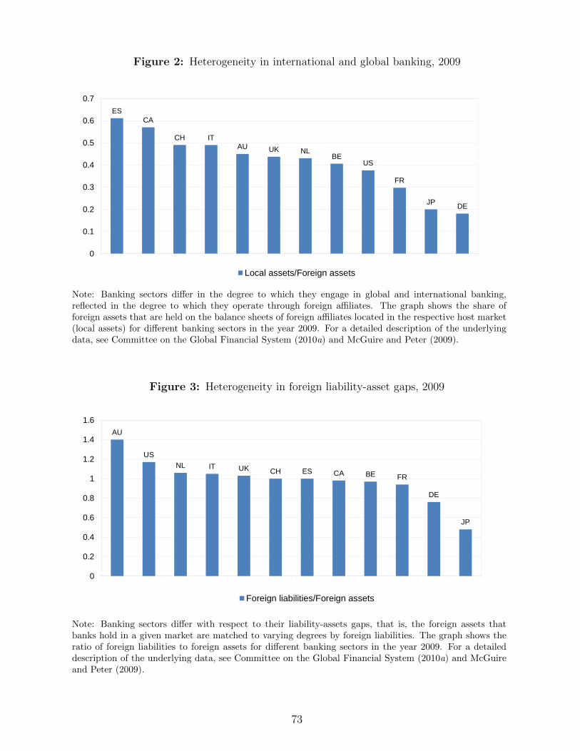
Figure 2: Heterogeneity in international and global banking, 2009

ESCA

CH ITAU UK NL

BEUS

FR

JPDE

0

0.1

0.2

0.3

0.4

0.5

0.6

0.7

Local assets/Foreign assets

Note: Banking sectors differ in the degree to which they engage in global and international banking,reflected in the degree to which they operate through foreign affiliates. The graph shows the share offoreign assets that are held on the balance sheets of foreign affiliates located in the respective host market(local assets) for different banking sectors in the year 2009. For a detailed description of the underlyingdata, see Committee on the Global Financial System (2010a) and McGuire and Peter (2009).

Figure 3: Heterogeneity in foreign liability-asset gaps, 2009

AU

US

NL IT UK CH ES CA BE FR

DE

JP

0

0.2

0.4

0.6

0.8

1

1.2

1.4

1.6

Foreign liabilities/Foreign assets

Note: Banking sectors differ with respect to their liability-assets gaps, that is, the foreign assets thatbanks hold in a given market are matched to varying degrees by foreign liabilities. The graph shows theratio of foreign liabilities to foreign assets for different banking sectors in the year 2009. For a detaileddescription of the underlying data, see Committee on the Global Financial System (2010a) and McGuireand Peter (2009).

73

Figure 4: Heterogeneity in foreign bank participation, 2009

NZL

FIN

BEL

DNKAUTNORKORGRCPRTUSACYPDEU

KWTGBRFRAITACANCHEAUSESPNLDARESWEISR

ESTBIHLTUSVKHRV

ROMCZEBGR

YUGLVAMKD

GEOHUNPOL

MDA

SVN

BLR

AZE

JAMSLV

MEX

NIC

TTOPER

HNDCRIPRYCHL

ARGGTM

BOLDOMCOL

ECU

ARM

KHM

PAKBHR

IDN

TURKAZMYSRUS

THAINDBGDVNMCHNJPN

ZMBMDGMOZBFA

UGASWZ

TZABWA

GHAAGO

KENMARNAM

MWIEGYDZAZAFSYC

NPLSDN

NGA

0

20

40

60

80

100

120Foreign bank participation in %

Advanced Emerging Europe Latin America Asia Africa

Note: Countries differ in foreign bank participation. The graph displays the share of lending by foreignbanks in total domestic lending for different countries in the year 2009. For information on the underlyingdata, see Claessens and van Horen (2012).

74

Figure 5: Four banking activities

Firm i

Depositors i

Firm j

Depositors j

Bank i Bank j

Panel 1: Domestic Banking

Firm j

Panel 2: International Banking

Firm i

Bank i Bank j

Depositors i Depositors j

Firm i

Bank j Bank i Bank j

Depositors i

Firm j

Depositors j

Bank i

Panel 3: Global Banking

Firm j

Panel 4: Foreign Sourcing

Firm i

Depositors i Depositors j

75

Figure 6: Equilibrium types

 

Δ a 

Δ (K/L)

1.No trade 

2. International 

banking j 

3. Foreign 

sourcing j 

4. International and global 

banking j 

5. Foreign sourcing and 

global banking j 

6. Foreign 

sourcing j and 

international 

banking i 

7. International banking 

i 

Note: The graph shows how the equilibrium type changes as the parameter values of ∆a and ∆(K/L)vary. The following parameters are chosen for the numerical example: τ ij = τ ji = 0.02, tij = tji =0.04, Ki = 20, Kj = 20, Lj = 10, Li ∈ [6, 23], ai ∈ [0.22, 0.4], aj = 0.25, z = 3, γ = 4. Theproduction function is Cobb-Douglas with a labor share of 0.3.

76

Figure 7: Bank-to-bank lending

Firm i

Bank j

Depositors i

Firm j

Depositors j

Bank i

ABji>0, LIij>0

77

Figure 8: Overhead costs and capital-labor ratios across countries, 2000

ARE

ARG

AUS

AUT

BDI

BEL

BENBGD

BHR

BLZ

BOL

BRA

BRB

BWA

CAN

CHE

CHL

CHN

CIVCMR

COG

COLCRI

CUB

CYP

DEU

DNK

DZA

ECU

EGY

ESP

FIN

FRA

GAB

GBR

GHA

GTMHND

HUN

IDN

IND

IRLIRN

ISL

ISR

ITA

JOR

JPN

KEN

KOR

KWT

LKA

LSO

MAC

MAR

MEX

MLI

MLT

MNG

MOZ

MRT

MUS

MWI

MYS

NER

NIC

NLDNOR

NPLPAK

PAN

PER

PHL

POL

PRT

PRY

QAT

ROU

SAU

SDN

SEN SLE

SLV

SWE

SWZ

THA TTO

TUN TUR

UGA

URY

USA

VEN

ZAF

ZMB

ZWE

020

4060

Cap

ital-l

abor

rat

io

0 .05 .1 .15Overhead costs to total assets

Note: The graph shows for each country in the sample the respective the ratio of overheadcosts to total assets (x-axis) of the domestic banking sector and its human-capital adjustedcapital-labor ratio (y-axis).

78