K.7

Banking Across Borders With Heterogeneous Banks Niepmann, Friederike

International Finance Discussion Papers Board of Governors of the Federal Reserve System

Number 1177 August 2016

Please cite paper as: Niepmann, Friederike (2016). Banking Across Borders With Heterogeneous Banks. International Finance Discussion Papers 1177. http://dx.doi.org/10.17016/IFDP.2016.1177

Board of Governors of the Federal Reserve System

International Finance Discussion Papers

Number 1177

August 2016

Banking Across Borders With Heterogeneous Banks

Friederike Niepmann NOTE: International Finance Discussion Papers are preliminary materials circulated to stimulate discussion and critical comment. References to International Finance Discussion Papers (other than an acknowledgment that the writer has had access to unpublished material) should be cleared with the author or authors. Recent IFDPs are available on the Web at www.federalreserve.gov/pubs/ifdp/. This paper can be downloaded without charge from the Social Science Research Network electronic library at www.ssrn.com.

Banking Across Borders With Heterogeneous Banks∗

Friederike Niepmann†

July 19, 2016

Abstract

This paper develops a model of banking across borders where banks differ in their

efficiencies that can replicate key patterns in the data. More efficient banks are more

likely to have assets, liabilities and affiliates abroad and have larger foreign operations.

Banks are more likely to be active in countries that have less efficient domestic banks,

are bigger and more open to foreign entry. In the model, banking sector integration

leads to bank exit and entry and convergence in the return on loans and funding

costs across countries. Bank heterogeneity matters for the associated welfare gains.

Results suggest that differences in bank efficiencies across countries drive banking across

borders, that fixed costs are crucial for foreign bank operations and that globalization

makes larger banks even larger.

Keywords : cross-border banking, heterogeneity, multinational banks, trade in services

JEL-Codes : F12, F21, F23, G21

∗The author is grateful to Andrew Bernard, Giancarlo Corsetti, and Russell Cooper for advice and en-couragement. For their helpful comments, she also thanks Silja Baller, Dean Corbae, Frederic Malherbe,Stefania Garetto, Francesc Ortega, John Romalis, Katheryn Russ, Tim Schmidt-Eisenlohr, Jan-Peter Sied-larek, and participants in seminars at the Federal Reserve Bank of New York, the European UniversityInstitute, the University of Oxford, the Inter-American Development Bank, UC Davis, ECB and the FDIC.Special thanks go to Cornelia Kerl, the Research Division and the Research Data and Service Centre of theDeutsche Bundesbank, where part of this paper was written while Niepmann was a visiting researcher. Theauthor also thanks Ina Simonovska for making available some of the data used in this research.†The author is a staff economist in the Division of International Finance, Board of Governors

of the Federal Reserve System, Constitution Avenue NW, Washington, D.C. 20551, USA. Email:Friederike.Niepmann@frb.gov. The views in this paper are solely the responsibility of the author and shouldnot be interpreted as reflecting the views of the Board of Governors of the Federal Reserve System or of anyother person associated with the Federal Reserve System.

1 Introduction

Banks today run large foreign operations. At the end of 2014, the foreign assets of banks

from 30 BIS reporting countries accounted for 36 percent of their total assets, exceeding

$26 trillion.1 But there is substantial heterogeneity across banks in the geographic coverage

and volume of their foreign operations.2 As Figure 1 shows, German banks with foreign

operations had lower overhead costs to total assets, an inverse measure of efficiency, than

the average bank.3

This paper presents a general equilibrium model of trade in banking services and financial

sector foreign direct investment that sheds light on the drivers of banks’ foreign operations,

explains the observed heterogeneity and explores the implications of banking sector integra-

tion. Using elements from Niepmann (2015) and Holmstrom and Tirole (1997), the model

links banks’ efficiency and size to their foreign operations in an open economy setup where

banking across borders arises from differences in marginal products of capital and banking

sector efficiencies across countries. The proposed model is consistent with key empirical reg-

ularities in the data, concerning both the extensive and intensive margin of banks’ foreign

operations.

In the model, banks have two roles. First, they channel capital from depositors to firms.

Second, they monitor firms at a cost. Whether banks monitor is not observable by depositors

so to credibly commit to monitor, banks invest their own capital in the firms they lend to.

Banks with lower monitoring costs are able to intermediate more external capital for the

same amount of equity capital and make higher profits.4

This microstructure carries over to the open economy where countries can differ in their

relative endowments of capital and labor, production technologies and banking sector effi-

ciencies. These differences cause the return on loans that banks earn and the rate on deposits

they pay to vary across countries. When banking sectors integrate, banks lend and borrow

1These numbers are based on data from the Consolidated Banking Statistics provided by the BIS on anultimate risk basis. See http://stats.bis.org/statx/srs/table/b1?p=20144&c=.

2Equivalent relationships have been documented in depth for manufacturing firms. See Bernard et al.(2012) for a recent survey of empirical works on firm heterogeneity and international trade.

3For details on the underlying data, see section 5.4In the model, bank capital is fixed and cannot relocate from one bank to the other preventing the most

efficient bank from serving the entire market.

1

across borders to maximize the return on loans and to minimize funding costs.

Banks have the choice between two different modes to serve foreign markets. They can

either lend and borrow cross-border, or they can establish an affiliate abroad (invest in FDI).

It is assumed that the fixed costs of cross-border lending and borrowing are lower than the

fixed cost of FDI and that banks save on variable costs by opening up a foreign affiliate. As

more efficient banks have larger lending volumes and make higher profits, only they are able

to cover the higher fixed costs. Therefore sorting occurs: the most efficient banks establish

foreign affiliates abroad, while less efficient banks engage only in cross-border lending and

borrowing. Banks at the lower end of the efficiency distribution remain domestic.5

When the two banking sectors become integrated and banks borrow and lend across

borders, intermediation costs and returns to capital converge. Capital relocates from the

capital abundant/low technology country to the capital scarce/high technology country. In

the country that hosts the more efficient banking sector, new banks enter. In the other coun-

try, the least efficient banks exit as foreign banks intermediate local deposits. Because banks

that go global can increase their return on loans and lower their funding costs, their balance

sheets expand. Through these mechanisms, banking across borders affects the equilibrium

bank size distribution, which tends to become more unequal. A simulation of the model

shows that the welfare gains from banking sector integration depend on the degree of bank

heterogeneity in the liberalizing countries, illustrating the relevance of taking efficiency and

size differences across banks into account.6

The empirical analysis draws on information on the external positions of banks and

bank balance sheets for 2005 available at the Deutsche Bundesbank.7 They contain detailed

information on the foreign activities of all German banks and their affiliates in a large number

of countries. As a proxy for the efficiency of single banks, I use two simple accounting

measures: a bank’s overhead costs as a ratio to total assets and labor productivity. 99

5This is similar to Melitz (2003) and Helpman et al. (2004) where manufacturing firms sort into FDI andexporting according to their productivity levels.

6In contrast to this paper, the model in Niepmann (2015) with perfectly competitive, homogenous banks,predicts equal welfare gains when average intermediation costs in the integrating countries are the same.

7Research Data and Service Centre of the Deutsche Bundesbank, External Position of Banks (AUSTA- “Auslandsstatus der Banken”), Monthly Balance Sheet Statistics (BISTA - “Monatliche Bilanzstatistik”),Income and Loss Data (GuV - “Gewinn und Verlustrechnung der Banken”), 2005.

2

percent of German banks have assets in foreign countries. However, most banks have assets

and liabilities in only a handful of countries, while the top German banks cover more than

150 countries. Operating affiliates abroad is much less common. Only 2.6 percent of German

banks have affiliates and these affiliates span only 58 different countries.

Beyond establishing these facts, the derived dataset is used to support key predictions

of the model. A first set of regressions explores the role of bank efficiency for balance sheet

sizes and foreign operations. First, banks with lower overhead cost are larger and more

levered. Second, as indicated in figure 1, banks with lower overhead costs are more likely

to have cross-border assets, cross-border liabilities and affiliates in foreign countries. Third,

conditional on operating abroad, the volume of their foreign activities is larger.

The model also predicts how the operations of banks vary with foreign country charac-

teristics. Specifically, the number of firms that are active abroad should increase with the

size of a country and decrease with the efficiency of its banking sector as well as the fixed

and variable costs of operating there. Logit regressions, where the dependent variable takes

a value of 1 if a bank k has foreign assets, liabilities or affiliates in country i confirm that

German banks are more likely to operate in countries with a larger GDP, a less efficient

banking sector, higher bureaucratic quality and financial freedom and a smaller geographic

distance. The sorting of banks into foreign markets based on their efficiency and host coun-

try characteristics is so strong that these factors explain the vast portion of the variation in

the average efficiency and the minimum efficiency of German banks that operate in various

foreign countries.

The presented results have several implications. The fact that the average efficiency of

banks that operate in country i increases with the efficiency of the banking sector in country

i strongly suggests that differences in intermediation costs across countries are a key driver

of banking across borders. Second, the stark sorting pattern indicates that foreign bank

activities are associated with substantial fixed costs, which only banks with larger operating

volumes are able to overcome. Third, banking across borders allows banks to grow their

balance sheets. Since only the largest banks are active abroad, banking sector integration

tends to make large banks even larger. Finally, bank heterogeneity matters since it influences

how banking sector integration affects net interest rate margins, capital flows and welfare.

3

Related Literature This research contributes to the small but growing literature on cross-

border banking. Similar to Niepmann (2015), this paper takes a trade approach where

differences in relative factor endowments and financial intermediation technologies across

countries drive banking across borders. In contrast to the aforementioned work, the frame-

work presented here exhibits imperfect competition and allows for bank-level heterogeneity.

A few other papers also study the effects of increased competition and banking sector

integration in the presence of heterogeneous banks. Ennis (2001) incorporates a moral hazard

problem at the side of bankers in a multi-regional banking model, focussing on the effect

of integration on the size distribution of banks. In his model, banks differ with respect to

equity, in contrast to the efficiency differences modeled here. Banking across regions allows

the bank with the largest equity to diversify lending, which relaxes information problems

and increases profits.

De Blas and Russ (2010, 2012) study the effects of financial liberalization on banks’ loan

pricing and the distribution of markups.8 The former paper relies on a structure where banks

offer differentiated services in line with Bernard et al. (2003). In the latter work, banks with

different efficiencies coexist, as not all firms can visit the most efficient bank. Cross-border

lending arises because firms apply for loans also at foreign banks to minimize expected costs.

FDI and cross-border lending are analyzed as separate scenarios.

Corbae and D’Erasmo (2010) propose a DSGE model to study the effect of bank com-

petition on bank market structure, entry and exit and the riskiness of bank loans along

the business cycle, distinguishing between regional and global banks. In an application of

that model, Corbae and D’Erasmo (forthcoming) evaluate the welfare effects of foreign bank

entry in Mexico. Recently, Fillat et al. (2015) provide a structural model with bank het-

erogeneity, analyzing how banks’ mode of entry (through either branches or subsidiaries)

affects the transmission of foreign shocks to the United States. Kerl and Niepmann (forth-

coming) simplify the model in this paper to explain the sectoral composition of international

bank flows, distinguishing between interbank market activity and cross-border business with

non-banking firms and households.

More broadly this research adds to the literature on heterogeneous firms in international

8De Blas and Russ (2010) is an earlier version of De Blas and Russ (2012).

4

trade and investment. The proposed theoretical structure differs substantially from existing

work-horse models with firm heterogeneity. In the class of models following Melitz (2003),

heterogeneous manufacturing firms produce differentiated goods as a result of consumers’

love for variety and labor, the only production factor is immobile. In this paper instead,

banks provide a homogenous intermediation service and move capital across borders. In

this regard, this work also contributes to services trade research (see Francois and Hoekman

(2010) for a literature review).

The assumptions on fixed and variables costs that banks face follow Helpman et al. (2004)

and result in a similar concentration-fixed-cost tradeoff here. Buch et al. (2014) and Lehner

(2009) model such a tradeoff for banks in partial equilibrium frameworks in contrast to the

general equilibrium approach in this paper.

This work also extends the empirical literature on cross-border banking. Several pa-

pers have analyzed how country characteristics affect the foreign activities of banks (see,

for example, Papaioannou (2009); Buch (2003); Buch (2005); Focarelli and Pozzolo (2005)).

Niepmann (2015) shows that the foreign positions of banks are determined by differences in

relative factor endowments and banking sector efficiencies between countries. Buch et al.

(2011) introduce the dataset explored in this paper, documenting that the foreign operations

of German banks vary systematically with their size and productivity.9 The empirical anal-

ysis in this paper complements these works, in particular by analyzing the sorting of banks

into foreign activities based on host country characteristics.

The paper is structured as follows. Section 2 presents the closed economy model. Section

3 discusses the open economy setup. Section 4 solves the model analytically and simulates

it for the case where relative factor endowments and production technologies are the same

across countries. Section 5 explores patterns in the German bank-level data. Section 6

concludes.

9For follow-up version of that paper, see Buch et al. (2014).

5

2 The Closed Economy Model

2.1 Setup

There is a continuum of capitalists of measure K, who can become bankers or depositors, and

a continuum of workers of measure L. Each capitalist is endowed with one unit of capital.

Each worker supplies inelastically one unit of labor. Furthermore, there is a continuum of

potential entrepreneurs who can run firms. Firms are perfectly competitive and produce

a single consumption good using capital and labor. Each firm operates under the same

constant returns to scale technology. The production function takes the form F (A, l, z). A

is a productivity parameter and F (A, l, z) is assumed to be a continuous function, strictly

increasing and concave in l. The capital input per firm z is fixed.10

There are two periods: in the first period, investments are made. In the second period,

firms produce. With probability λ, production is successful so that capitalists and workers

are paid and consume. It is useful to determine equilibrium factor prices first. In equilibrium,

all capital is employed in production, which implies that the measure of operating firms is

N = K/z.11 As firms compete for labor and are symmetric, they employ the same amount

of labor l. Labor market clearing implies that l = L/N . Under perfect competition, the

returns to the production factors are pinned down by their marginal products. The gross

return to capital is R = (1 + Fz(1, z/l)) = (1 + FK(1, K/L)). The wage rate is given by

w = FL(1, K/L).

Each capitalist decides whether to become a banker or a depositor in the first period.

Bankers have two tasks in the economy: first, they channel capital from depositors to firms.

Second, they monitor the firms they lend to at a cost to increase the probability that produc-

tion is successful. As the suppliers of capital, bankers collect the gross return to capital R in

the second period. Depositors invest their endowments in banks and obtain the return RD,

which is endogenously determined. Before each capitalist makes his occupational choice, he

learns about his efficiency as a banker. Each capitalist draws a monitoring cost γ > 0 from

10Instead of fixing z exogenously, one could endogenously limit the size of a single firm by formulating themoral hazard problem at the side of the entrepreneur similar to Ju and Wei (2010).

11Capitalists do not have available a storage technology.

6

a continuous distribution g(γ) with support γ ∈ [γ, γ]. The lower the cost draw the higher

the capitalist’s efficiency as a banker.

The role of monitoring and incentive problems in the model is similar to the framework in

Holmstrom and Tirole (1997) with double-sided moral hazard. First, the success probability

of the firm depends on the effort exerted by the entrepreneur. With effort, the success

probability is λ. Without effort, it is λL < λ. Only monitoring by banks induces the

entrepreneur to exert effort.

Second, bankers only monitor if they have an incentive to do so.12 To credibly commit to

monitor, a banker invests his own capital in the firms he lends to.13 Incentive compatibility

requires that the banker’s expected return under monitoring is higher than the return without

monitoring, which results in the following condition:

λRz − λRD(z − v)− γz ≥ λLRz − λLRD(z − v), (1)

where γz are the total monitoring costs incurred and v represents the banker’s capital (equity)

invested in the firm. To maximize profits, each banker maximizes the number of firms he

monitors and lends to. This implies minimizing v.14 Therefore, in equilibrium, condition 1

holds with equality. Solving the condition for bank capital v(γ) yields:

v(γ) =

(1− R

RD+

γ

(λ− λL)RD

)z. (2)

The model puts some discipline on the magnitude of monitoring costs. Monitoring costs

are assumed to be sufficiently low so that all firms are monitored by banks and operate with

a high probability of success in equilibrium. At the same time, monitoring costs have to

be sufficiently high so that the incentive compatibility constraint of even the most efficient

12Depositors do not observe whether bankers monitor but can observe a banker’s monitoring cost (type)γ.

13It is assumed that the success of firms is perfectly correlated so that banks must invest their own capitalto solve the moral hazard problems. See Holmstrom and Tirole (1997).

14To see this, substitute n = 1/v in the expression for total profits to obtain π = n(λRz−λRDz−γz)+λRD.

7

banker γ binds in equilibrium.15

As bank capital v(γ) invested per firm is proportional to the capital input z of the firm, z

is normalized to 1. The return of a banker with monitoring cost γ per firm that he monitors

and lends to is then obtained as:

λR− λRD(1− v(γ))− γ =γλLλ− λL

. (4)

The number (measure) of firms that one banker endowed with one unit of capital can monitor

is n(γ) = 1v(γ)

.16 The higher a banker’s monitoring efficiency, that is, the lower γ, the

more external capital he channels from depositors to firms and the larger his balance sheet

becomes.17 A banker of type γ operates under the following leverage:

debt

equity=

depositor capital

bank capital=n(γ)x(γ)

1=

1

v(γ)− 1, (5)

where x(γ) = 1− v(γ) is the depositor capital that a banker of type γ lends to a single firm.

Profits of the banker of type γ are given by:

π(γ) = n(γ)(λR− λRD(1− v(γ))− γ) =1

v(γ)

γλLλ− λL

=1

1− RRD + γ

(λ−λL)RD

γλLλ− λL

. (6)

The return that the banker makes per firm, which corresponds to the second term in expres-

sion (6), depends only on the banker’s monitoring cost γ and on the success probabilities

λ and λL. These parameters are exogenous and fixed. The lower γ, the higher λ and the

15Sufficient conditions are:∫ γ=R(λ−λL)

γ

(1

1− λλL

+ γλ(λ−λL)λLR

− 1

)g(γ)dγ >

∫ γ

γ=R(λ−λL)

g(γ)dγ. (3)

and γ > (λ− λL)R(1− λL

λ ). The first condition requires that at the deposit rate RD = λL/λR, the demandfor external funds by bankers is larger than the supply of funds by depositors to bankers. This ensures thatin equilibrium RD > λL/λR and γ∗ < R(λ − λL). The second condition requires that at the deposit rateRD = λL/λR, the incentive compatibility constraint is binding for the most efficient banker. From theseconditions, it follows that in equilibrium, λR− γ ≥ λRD ∀γ ≤ γ∗ and λRD > λLR.

16Integer problems are ignored. One firm may borrow from several banks.17The relationship between efficiency, bank size and leverage in the model is consistent with the data as

shown in section 5.3. See also Kalemli-Ozcan et al. (2012) who find that larger banks have a higher leverage.

8

lower λL are, the higher are the banker’s profits. The endogenous variables of the model,

R and RD, affect profits only through the measure of firms n(γ) that the banker serves, i.e.

through the lending volume, and, as bank capital is fixed, through leverage. The banker’s

lending volume and profits increase with the gross return to capital R.18 Profits decrease

with the the cost of external funding RD.19

While the profits of a banker depend on his type γ, all depositors are paid the same

return. This is because the monitoring cost draw of a depositor is assumed to remain private

information in contrast to the draw of a banker.

2.2 Equilibrium

Two equilibrium conditions close the model. First, there is free entry into banking. Second,

the market for financial intermediation clears, i.e. all operating bankers in the economy

intermediate capital K.

First, consider free entry into banking. Each capitalist has the choice between becoming

a banker or a depositor. The marginal capitalist γ∗ who is indifferent between the two

occupational choices is determined by setting the expected profits of a capitalist as a banker

equal to his expected profits as a depositor:

π(γ∗) =1

1− RRD + γ∗

(λ−λL)RD

γ∗λLλ− λL

= λRD. (7)

Because profits are strictly decreasing in γ, all capitalists for whom γ > γ∗ become depositors

and those for whom γ ≤ γ∗ become bankers.

All active bankers together must intermediate the existing capital in the economy. The

economy is endowed with capital of measure K. A banker of type γ is able to supply a

measure of n(γ) firms with capital. Thus the market for financial intermediation clears if:

K

∫ γ∗

γ

n(γ)g(γ)dγ = K. (8)

18A shock to productivity A increases R. Thus, lending, leverage and profits are procyclical in line withthe empirical evidence. See e.g. Adrian and Shin (2014).

19Because λR− λLR− γ > 0 ∀γ < γ∗, the derivative of π(γ) with respect to RD is always negative.

9

Equations (7) and (8) constitute a system of two equations in two unknowns RD and γ∗,

which fully determine the equilibrium. Solving equation (7) with respect to RD yields:

RD = R− γ∗

λ= (1 + FK(1,

K

L))− γ∗

λ. (9)

The return to depositors RD depends on the marginal product of capital (MPK) and, there-

fore, on the relative factor endowments of the economy, as well as on banking sector efficiency

reflected in γ∗. The lower banking sector efficiency in the economy, the larger the wedge

between the gross return to capital R and the return on deposits RD becomes.20

Plugging the expression for RD into the market clearing condition (8) delivers:

1 =

∫ γ∗

γ

(R− γ∗

λ)(λ− λL)

γ − (λ− λL)γ∗

λ

g(γ)dγ. (10)

Expression (10) implicitly gives a solution for the bank entry cutoff γ∗.

Proposition 1 The solution γ∗ to

1 =

∫ γ∗

γ

(R− γ∗

λ)(λ− λL)

γ − (λ− λL)γ∗

λ

g(γ)dγ (11)

is unique and exists under the sufficient conditions:

∫ γ=R(λ−λL)

γ

1

1− λλL

+ γλ(λ−λL)λLR

g(γ)dγ > 1, (12)

and

γ > (λ− λL)R(1− λLλ

). (13)

Proof. See appendix A.

The equilibrium cutoff γ∗ is a function of the parameters of the model. The lower the

gross return to capital R is, the smaller is the amount of external capital a single banker can

20This is similar to Antras and Caballero (2009) and Ju and Wei (2010).

10

intermediate. As a consequence, the bank entry cutoff increases with the capital-labor ratio

K/L and decreases with productivity A. In addition, the bank entry cutoff is affected by

changes in the monitoring cost distribution. The more efficient the banking sector is overall,

the fewer banks are needed to intermediate the available capital in the economy and the

lower is γ∗.

3 The Open Economy Model

3.1 Setup

In the open economy, there are two countries home (h) and foreign (f), which can differ in

their relative endowments of capital and labor, in the productivity of domestic firms and in

aggregate banking sector efficiency so that autarky returns to capital R and deposit rates

RD may vary across countries.

Workers, entrepreneurs and depositors are assumed to be immobile.21 In contrast, banks

can operate in both countries. They have the choice between raising deposits at home and

abroad and between investing at home and abroad. Operating internationally is costly,

however. If a banker in country j ∈ {h, f} wants to extend loans to firms in country

i ∈ {h, f} where i 6= j, he has to incur the fixed cost fLij > 0. If he wants to borrow from

foreign depositors, he has to pay the fixed cost fBij > fLij . Once fBij is incurred, the banker

does not have to pay an extra cost to extend cross-border loans.22 In addition to fixed costs,

the banker also faces variable costs, which take the form of “iceberg” costs. If the gross

return Ri is collected in country i, only a fraction of the return, τRi, where τ < 1, arrives at

the bank in country j. At the same time, for the return RDi to go to depositors in country

i, φRDi units have to be transported, where φ > 1.23 Banks can eliminate variable costs by

21In reality, a share of financial investors is mobile. However, some investor capital may become mobileonly through banks. This should in particular be true for deposits, which represent an important fundingsource for banks.

22Alternative fixed cost structures could be modeled. This structure implicitly assumes that there aresynergies between borrowing and lending.

23In models of goods trade, iceberg costs reflect variable trade costs that increase in the distance betweenthe importing and the exporting country. Degryse and Ongena (2005) find that distance-related transporta-tion costs matter also in banking, in support of the modeling choice here. See Brevoort and Wolken (2009)for a summary of the literature on the role of distance in banking.

11

opening up an affiliate abroad. However, establishing a foreign affiliate (making a foreign

direct investment, FDI) requires paying a higher fixed cost fAij > fBij .

The profits of a banker in country j who raises deposits at home and invests them in

country i through cross-border lending are given by:

πXij (γj) = n(γj, τRi, RDj )

γjλL

λ− λL− fLij =

1

1 + 1RD

j( γλ−λL

− τRi)

γjλL

λ− λL− fLij . (14)

The first subscript in πXij stands for the country to which the banker lends. The second

subscript indicates where capital is raised. Superscript X indicates that the banker operates

cross-border rather than through an affiliate which is denoted by superscript A. n(γj, Ri, RDj )

reflects the total capital that the banker of type γj intermediates, which depends on his

monitoring cost γj, the gross return to capital he collects and the deposit rate he has to pay.

Accordingly, a banker that raises deposits abroad to finance lending at home collects:

πXji(γj) = n(γj, Rj, φRDi )

γjλL

λ− λL− fBij =

1

1 + 1φRD

i( γλ−λL

−Rj)

γjλL

λ− λL− fBij . (15)

If instead the banker borrows from depositors abroad and lends to firms abroad (local inter-

mediation), his profits are:

πXii (γj) =1

1 + 1φRD

i( γλ−λL

− τRi)

γjλL

λ− λL− fBij . (16)

Finally, the entrepreneur can invest in FDI. In this case, τ and φ are equal to one, and the

fixed cost is replaced by fAij in the last three equations.

Each banker chooses between the seven options (πjj, πXij , π

Xii , π

Xji , π

Aij, π

Aii , and πAji) taking

the gross returns to capital Ri and Rj, the returns on deposits RDi and RD

j as well as costs

as given.

12

3.2 Sorting

It is useful to establish a key result of the model before defining the equilibrium in the

open economy: bankers sort into cross-border lending, borrowing and FDI according to their

monitoring cost γ.

Consider the general profit function:

π(R,RD, γ, τ , φ) =1

1− τRφRD + γ

(λ−λL)φRD

γλLλ− λL

. (17)

Substitute RD = φRD and R = τR. The function π(R, RD, γ) is supermodular in γ and

−R and in γ and RD, i.e. π−R,γ > 0 and πRD,γ > 0. Mrazova and Neary (2011) show that

supermodularity is a sufficient condition for sorting in a way that the high-efficiency banks

engage in the activity that requires paying the (higher) fixed cost, whereas low-efficiency

banks engage in the activity with no (the lower) fixed cost. This result facilitates the

equilibrium computation because once the banker who is indifferent between two activities

is found, the decisions of all other active bankers follow immediately.

Proposition 2 If bankers of different types engage in different activities in equilibrium, then

sorting is such that the most efficient bankers sort into the activity that requires paying the

(higher) fixed cost while the low efficiency bankers engage in the activity with no (the lower)

fixed cost.

Proof. See appendix A.

In the following, γLj (γBj ) denotes the cross-border lending (borrowing) cutoff, that is, all

bankers with γj ≤ γLj (γBj ) find it profitable to lend (borrow) across borders. Similarly, all

bankers with γj ≤ γAj find it profitable to operate in country i by establishing an affiliate

there. A banker is only willing to pay a fixed cost if he can collect a higher return on the

loan or obtain cheaper funding abroad. Once the cost is incurred, it is optimal for the banker

to invest all capital in the high return location and to raise all deposits in the low-interest

country. Similarly, if a bank opens up a foreign representation, it conducts all business

through the foreign affiliate to save on variable costs.24

24Bankers will always choose to raise deposits either at home or abroad. They will also, in general, either

13

Because more efficient banks are larger, that is, they borrow and lend more, they also

hold more cross-border assets, cross-border liabilities as well as more assets and liabilities in

their foreign affiliates. The model therefore predicts not only that the extensive margins of

banking across borders co-vary positively with bank efficiency but also the different intensive

margins.

Corollary 1 Bankers with lower monitoring costs are more likely to lend and borrow abroad

and to have foreign affiliates. Conditional on operating abroad, their foreign operations have

higher volumes.

3.3 Equilibrium definition

The equilibrium in the open economy is defined as follows:

Definition 1 An equilibrium in the open economy is characterized by the bank entry cutoff

γ∗j , the cross-border lending cutoff γLj , the cross-border borrowing cutoff γBj , the FDI cutoff

γAj , returns to depositors RDj and gross returns to capital Rj for j ∈ {h, f}, i ∈ {h, f} and

j 6= i for which the following conditions hold:

(i) Capitalists in each country optimally choose whether to become depositors or bankers.

(ii) Bankers in each country optimally choose to lend at home and abroad.

(iii) Bankers in each country optimally choose to raise capital at home and abroad.

(iv) Bankers in each country optimally choose between the two modes of operating abroad

(cross-border versus FDI).

(v) Capital flows are consistent with the choice of bankers to invest and to raise capital

abroad.

(vi) Labor markets clear.

(vii) All capital is employed in production (capital market clearing).

(viii) The market for financial intermediation clears.

invest at home or abroad. These results could be relaxed by introducing heterogeneous firms/depositorsleading to assortative matching or by including a motive for banks and depositors to diversify lending andborrowing.

14

4 Analytical Solution with KhLh

=KfLf

, Ah = Af , τ = 1

In the following, it is assumed that the two countries operate the same production technology

and have the same relative factor endowments, that is, Kh

Lh=

Kf

Lfand Ah = Af , but that

they differ in their banking sector efficiencies. As a result, autarky returns to capital are the

same while autarky deposit rates vary across the two countries. To make the model even

more tractable, τ is set equal to 1, that is, there are no variable costs associated with lending

across borders.

When technologies and returns to capital are the same in both countries, the allocation

of capital is efficient and, because of τ = 1, unaffected by banks’ foreign operations. Because

cross-border lending is costless once the fixed cost fB or fA have been incurred, banks will

always lend across borders so that gross returns remain equalized. As a result, the net capital

flow is zero in equilibrium and R can be taken as given and fixed.

Without loss of generality, the home country is assumed to host the more efficient banking

sector so that the autarky deposit rate is lower in the foreign than in the home country. This

gives home banks an incentive to raise funding in the foreign country. Monitoring costs are

assumed to be Pareto distributed with the same shape parameter a, γh ∈ [γh

= γ,∞] and

γf ∈ [γf

= γ + ∆,∞].

The notation can be simplified and subscripts dropped. The profits of a home banker

who raises deposits in the foreign country, borrowing cross-border without an affiliate, are

given by:

πX(γh) = n(γh, R, φRDf )

γhλLλ− λL

− fB =1

1 + 1φRD

f( γhλ−λL

−R)

γhλLλ− λL

− fB. (18)

Accordingly, the profits of a banker from the home country that raises deposits abroad

through a local affiliate are:

πA(γh) = n(γh, R,RDf )

γhλLλ− λL

− fA =1

1 + 1RD

f( γhλ−λL

−R)

γhλLλ− λL

− fA. (19)

15

4.1 Equilibrium

I focus on the interesting case of an interior solution. For this, ∆ cannot be be too big.

Moreover, size differences cannot be too large so that some capitalists in the foreign country

operate as bankers in the open economy equilibrium and not all capitalists in the home

country become bankers. To exclude autarky as the equilibrium, variable and fixed costs

cannot be prohibitively high. Due to the complexity of the model, it is not possible to

characterize the exact parameter space for which an interior solution results although it is

easy to come up with examples. If there is an interior solution, it is unique.

The result on sorting derived in the previous section implies that home bankers will sort,

in such an equilibrium, into cross-border borrowing and FDI according to their monitoring

costs. Define γBh as the solution to πX(γh, φRDf , R) = π(γh, R

Dh , R) and γFf as the solution

to πF (γh, RDf , R) = max{π(γh, R

Dh , R), πX(γh, φR

Df , R)}.25 Then three cases are possible: in

equilibrium, (i) γh< γFh < γBh , (ii) γFh ≤ γ

h< γBh , or (iii) γ

h< γFh and γBh ≤ γFh . In case

(i), some home bankers borrow cross-border from depositors abroad, while other bankers use

affiliates for it. In case (ii), the fixed cost of FDI fA is too high for banks to establish foreign

affiliates in equilibrium. In case (iii), the fixed cost of FDI fA is relatively low so that all

banks that borrow from abroad establish foreign affiliates.

Let E denote the total equity of banks in the home country that borrow from abroad

and let D denote the deposits that these banks raise in the foreign country. Then an interior

solution is characterized by the following equations:

Kf −D = Kf

∫ γ∗f

γf

n(γf , R,RDf )gf (γf )dγf , (20)

Kh = E +Kh

∫ γ∗h

max{γAh ,γBh }n(γh, R,R

Dh )gh(γh)dγh, (21)

π(γ∗f ) = λRDf , (22)

π(γ∗h) = λRDh , (23)

πX(γBh ) = π(γBh ), (24)

πA(γAh ) = max{π(γAh ), πX(γAh )}, (25)

25Note that each profit function cuts the other ones at most once for permissible parameter values.

16

where:

E = Kh

∫ max{γAh ,γBh }

γh

gh(γh)dγh, (26)

and

D = Kh

∫ max{γh,γAh }

γh

(n(γh, R,R

Df )− 1

)gh(γh)dγh

+ Kh

∫ max{γAh ,γBh }

max{γh,γAh }

(n(γh, R, φR

Df )− 1

)gh(γh)dγh. (27)

Proposition 3 The solution to equations 20 to 27 is unique.

Proof. See appendix A.

Equations (20) and (21) are clearing conditions of the market for financial intermediation

in the home and the foreign country, respectively. Because banks in the home country raise

deposits D in the foreign country, foreign banks have to intermediate only Kf −D units of

capital. In turn, bankers in the home country that obtain additional funding from abroad,

have to intermediate the domestic capital Kh plus the additional capital D. Equivalently,

the equity capital E of bankers that raise funding in the foreign country, plus the funds

intermediated by purely domestic home country banks, have to equal the home country’s

capital stock, a condition stated in equation 21. The remaining equations determine the

bank entry cutoffs in the two countries γ∗h and γ∗f , the cross-border borrowing cutoff γBh

and the FDI cutoff γAh . Together, the conditions constitute a system of six equations in six

unknowns.

Because funding is cheaper in the foreign country than in the home country under autarky,

home country banks expand abroad by raising funds from foreign depositors in the open

economy. This leads to entry into banking at home and bank exit in the foreign country. As

a result, the bank entry cutoff γ∗h moves up, while γ∗f declines. Deposit rates equilibrate but

do not equate. A gap between funding costs RDh −RD

f > 0 in the open economy equilibrium

remains which is smaller than under autarky but large enough to give home country banks

an incentive to incur the fixed and variable costs to expand their operations to the foreign

country.

17

Banking sector integration has an effect on the size distribution of banks in both countries

not only through changes in the bank entry cutoffs but also through changes in the size of

individual banks. The more efficient home country banks that borrow from abroad, either

cross-border or through FDI, can grow their balance sheets due to lower funding costs.

The size of banks that only operate in the domestic market is also affected since deposit

rates change. Foreign banks become smaller, while home country banks that operate only

domestically also get bigger.

4.2 Model simulation

To further illustrate the key mechanisms of the model and to explore in detail the role

of bank heterogeneity, I provide a numerical example. Bank-level data from the Deutsche

Bundesbank, which is described and explored in detail in section 5, is used to select the

parameters for the simulation. In the example, Germany corresponds to the home country,

while the Czech Republic is the foreign country.

4.2.1 Parameters

The German bank-level dataset contains the ratio of overhead costs to total assets of roughly

2000 German banks in the year 2005, which is the preferred, inverse measure of efficiency

used also later in the empirical analysis in section 5. Overhead costs comprise salaries,

expenditures for office space, IT etc. and are independent of funding costs, consistent with

the formulation of monitoring costs in the model.

Because the model assumes that each bank is endowed with one unit of equity capital,

I adjust the bank-level dataset by multiplying each bank-level observation with bank equity

and estimate the monitoring cost distribution based on this modified version.26 The resulting

overhead cost distribution closely resembles the Pareto distribution. The shape parameter

of the Pareto distribution estimated via Maximum Likelihood is a = 0.55.27 The minimum

26For example, a bank with an overhead cost ratio of 3 percent with 100 units of equity capital will showup as 100 observations each with a 3 percent ratio.

27I exploit the fact that when a Pareto distribution is truncted, the resulting distribution is also Paretodistributed and has the same shape parameter.

18

value of the distribution γG

is set to the average overhead costs of the 100 least efficient

German banks, which results in γG

= 0.006317.28

Information on capital-labor ratios and returns to capital are based on data from David

et al. (2014). Values for the year 2000 are used to fix capital and labor endowments as well

as TFP.29 λ and λL, the success probabilities of projects with and without monitoring are

deep parameters of the model that govern the leverage of banks. The two parameters are

set so as to ensure that the sufficient conditions from proposition 1 hold. Specifically, I set

λ equal to 0.9 and λL to 0.85.

In 2000, the Czech Republic had a similar marginal product of capital as Germany

according to David et al. (2014), and it hosted less efficient banks than Germany based

on information from the World Bank’s Financial Development and Structure Dataset. The

open economy equilibrium will therefore correspond to case where German (home) banks

raise funding from Czech (foreign) banks and marginal products of capital equalize.

The monitoring cost distribution that Czech banks draw from has the same shape pa-

rameter as that of German banks (a = 0.55). The minimum value of the Pareto distribution,

however, differs across countries. From the Financial Development and Structure Dataset,

the difference between the average overhead costs of German and Czech banks was one per-

centage point in 2000. Accordingly, γC

is set so that the average overhead costs of Czech

banks are 1 percentage point higher than that of German banks in the closed economy. This

implies γC

= 0.0103436 or ∆ = 0.0040266.

To solve for the open economy equilibrium, values for the fixed and variable costs that

German banks face when operating in the Czech Republic (φ, fB and fA) are also needed.

Since only four German banks have affiliates in the Czech Republic in 2005, I do not model

affiliate lending and set the fixed cost of FDI fA to a prohibitively high value. Furthermore,

I assume φ = 1.001 and fB = 0.24. Table 1 summarizes the parameters for the simulation.

28The first and 99th percentile of the overhead costs distribution are dropped for this exercise.29David et al. (2014) provide the capital stock and MPKs based on the method suggested by Caselli

and Feyrer (2007) by which returns are computed using country specific prices of output, consumptionand investment. I use additional data on the labor force and assume a Cobb-Douglas production functionY = AKαL1−α with a capital share of α = 0.3 to back out A.

19

4.2.2 Autarky versus open economy

Column (1) of table 2 shows the solution to the closed economy for Germany and the Czech

Republic. The two countries have very similar gross returns to capital, while German banks

have lower overhead costs. This implies that a smaller fraction of capitalists in Germany

becomes bankers and that the average balance sheet size and leverage of active bankers are

higher in Germany than in the Czech Republic. Accordingly, the German deposit rate is

higher than the corresponding Czech rate in the closed economy.

Next, the open economy equilibrium is computed using conditions (20) to (25).30 Out-

comes are presented in column (2) of table 2. German banks raise funding from Czech

depositors when the two countries integrate and replace Czech banks as domestic financial

intermediaries. The least efficient Czech banks exit. At the same time, there is entry into

banking in Germany. Deposit rates equilibrate with the German deposit rate falling and the

Czech deposit rate rising.

In equilibrium, around 4.5 percent of German banks borrow and lend from Czech resi-

dents. This implies that more than 59 percent of loans to Czech firms come from German

banks. Note that the few German banks can have relatively high lending volumes in the

host country because the Czech economy is much smaller than the German. Loans to Czech

firms represent around 4.5 percent of German banks’ total loans.

The opening up also has implications for banking sector concentration. The top chart of

figure 2 depicts the balance sheet size of German banks as a function of their overhead costs.

The dashed line shows the relationship in the closed economy, the solid line is for the open

economy. Because German banks that borrow from Czech depositors pay lower interest,

they can increase their balance sheet size. As a result, German banking sector concentration

measured by the share of banking sector assets that are held by the top 10 percent of the

banks increases.31 Due to exit by the smallest Czech banks, the concentration of the Czech

30With only small differences in autarky marginal products of capital, the equilibrium is determined bythese conditions together with the condition Rf = Rh, which pins down the net capital flow.

31Janicki and Prescott (2006) document changes in the size distribution of U.S. banks from 1960 to 2005.Consistent with the theory in this paper, they show that over time a higher fraction of banking sector assetsis held by a small number of large banks. See McCord et al. (2014) for an update of Janicki’s and Prescott’sstudy.

20

banking sector goes down.32

Because marginal products of capital across countries in the closed economy are not

identical, there is a small net capital flow (-0.00108) from the Czech Republic to Germany

so that MPKs across the two countries equate. German banks borrow on net from Czech

residents. Importantly, net capital flows are not equal to gross capital flows. German banks

export equity capital. This capital outflow must be offset by an import of deposits from the

Czech Republic by German banks to keep gross returns equalized. The model thus generates

two-way capital flows and explains why capital may flow into a county in the form of financial

sector FDI and might leave again as depositor capital. The equilibrium gross deposit flow

from the Czech Republic to Germany corresponds to roughly 9.4 percent of Czech deposits.

Welfare in both countries increases, defined as the sum of the return to workers, bank

profits and deposits paid. While banking sector profits are shifted from the Czech Republic (-

65 percent) to Germany (+5.4 percent), the Czech economy gains overall because monitoring

costs are reduced and, hence, depositors are paid almost 20 percent more compared to the

closed economy. The relative welfare gain is significantly bigger for the Czech Republic than

for Germany.

4.2.3 Role of heterogeneity

Two experiments make clear that bank heterogeneity matters. In each experiment, the

shape parameter of the Pareto distribution for German banks is set to a = 0.75; that is,

the distribution of monitoring costs features less heterogeneity (is less dispersed) than in the

baseline. In the first case, γG

is set so that the closed economy deposit rate RDG in Germany

is unchanged. In the second case, γG

is chosen so that the average overhead costs of German

banks are the same as in the baseline closed economy (γG

= 0.0065267).

Consider the first case. Keeping the German closed economy deposit rate constant in the

face of less bank heterogeneity means that the lower bound of the overhead cost distribution

must move up (to γG

= 0.0066995). As a result, the share of German capitalists that

become bankers increases, while the average size of German banks decreases. Because the

32The concentration measure is computed without taking lending by foreign banks into account.

21

Czech economy now integrates with an economy with slightly less efficient banks, the open

economy deposit rate in the Czech Republic remains below that of the baseline scenario.

Fewer German banks raise funding in the country and fewer bank profits are shifted to

Germany. The welfare gains from integration are lower.

In the second case, the average overhead costs of German banks under autarky are

unchanged. With less heterogeneity but the same average overhead costs, the lower bound

of the Pareto distribution also must move up (γG

= 0.0065267). The closed economy bank

entry cutoff γ∗G moves down and hence the German closed economy deposit rate is higher

than in the baseline. For the open economy equilibrium, this implies that the fraction of

German banks that borrow from Czech depositors increases. The Czech equilibrium deposit

rate and welfare gains for the Czech Republic are higher.

These experiments demonstrate that the open economy equilibrium and the welfare gains

from integration depend on the exact monitoring cost distribution of banks in the two coun-

tries. Bank heterogeneity, which is a key feature of the data as section 5 shows, matters

also in theory. The framework in Niepmann (2015), which analyzes banking across borders

in a model with a representative banking sector, delivers identical welfare gains when the

observed closed economy average intermediation costs and deposit rates in the integrating

countries are the same.

4.3 Comparative statics

The data from the Deutsche Bundesbank provides information on the foreign operations

of individual German banks across foreign countries. On the one hand, these data can be

used to test corollary 1 of the model, which relates bank efficiency to the intensive and

extensive margins of banking across borders. On the other hand, the data can shed light

on how German banks’ activities vary across foreign countries. Motivated by the data, the

focus in this section is on analyzing how the open economy equilibrium varies with the

characteristics of the foreign country, keeping home country characteristics fixed. While the

model does not have a closed form solution, implicit functions theorems can be used to derive

the comparative statics around an interior equilibrium analytically.

22

The effects of foreign country size Consider first an increase in the size of the foreign

country, reflected in a higher endowment of this country that leaves its capital-labor ratio

unaffected so that Rf = Rh = R continues to hold. With a bigger foreign country, the same

volume of deposits intermediated by home country banks implies a higher foreign deposit

rate. As a result, more home bankers find it profitable to obtain funding abroad. The cross-

border borrowing cutoff γB and the FDI cutoff γA move up. The foreign asset and liability

holdings of the home country banking sector increase (see Proposition 4).

Proposition 4 When the foreign country increases in size reflected in a proportional in-

crease of Kf and Lf (leaving the country’s capital-labor ratio unaffected), the cross-border

borrowing cutoff γB, the FDI cutoff γA as well as foreign liabilities dfh of individual home

country banks increase.33

Proof. See appendix A.

The effects of foreign banking sector efficiency Next, assume that the foreign banking

sector becomes less efficient, reflected in an increase in ∆. As a consequence, the difference

in autarky deposit rates between the two countries rises. Lower funding costs in the foreign

country relative to the home country provide larger incentives for home banks to expand

abroad and borrow from depositors there. Therefore, the cross-border borrowing cutoff γB

and the FDI cutoff γA increase. Banks from the home country hold more foreign assets and

liabilities in equilibrium. Proposition 5 summarizes this result.

Proposition 5 When the efficiency of the foreign banking sector decreases, reflected in an

increase in ∆, the cross-border borrowing cutoff γB, the FDI cutoff γA as well as foreign

liabilities dfh of individual home country banks increase.34

Proof. See appendix A.

33In the model with τ = 1, the foreign assets of individual home country banks are not determined.However, in equilibrium, D = A, where A denotes the total foreign assets of home country banks. So totalassets of home banks abroad increase in foreign country size.

34See footnote 23.

23

The effects of barriers to bank entry and cross-border frictions Finally, the effects

of changes in the fixed and variable costs of foreign operations are presented. With a higher

variable cost φ and a higher fixed cost of cross-border borrowing fB, fewer home country

banks find it optimal to borrow from depositors abroad. As a consequence, the borrowing

cutoff γB goes down. An increase in the fixed cost of FDI has the opposite effect. The

higher fA, the fewer banks invest in FDI and the less capital in the foreign country is

intermediated by home country banks. This means a lower foreign deposit rate ceteris

paribus and thus increased incentives for home country banks to engage in cross-border

borrowing. The cross-border borrowing cutoff γA therefore increases in fA. These results,

summarized in proposition 6, resemble the classic proximity-concentration tradeoff prominent

in international trade theory (see Helpman et al. (2004)).

Proposition 6 (i) When the variable cost of cross-border borrowing φ increases, the cross-

border borrowing cutoff γB decreases and the FDI cutoff γA increases. (ii) When the fixed

cost of cross-border borrowing fB increases, the cross-border borrowing cutoff γB decreases

and the FDI cutoff γA increases.

(iii) When the fixed cost of establishing a foreign affiliate fA increases, the cross-border

borrowing cutoff γB increases and the FDI cutoff γA decreases.

Proof. See appendix A. Empirical evidence in support of the predictions stated in

propositions 4 to 6 is provided in section 5.

4.4 Solution to the general model

When countries differ both in autarky returns to capital and banking sector efficiencies, the

equilibrium can take different forms.35 The numerical example presented in the previous sec-

tion illustrates what happens when relative factor endowments and production technologies

differ only slightly across countries. Because banks that have incurred the fixed costs fB or

fA are free to invest at home and abroad, they will invest in the country with the higher

return to capital. If the volume of capital that these banks can channel across border is

35This does not mean that there are multiple equilibria. Instead the equilibrium is characterized by adifferent set of equations.

24

large enough, gross returns to capital will equate and the equilibrium will be characterized

by conditions (20) to (25) with the addition that the net capital flow Kfh is not zero but

determined by Rf = Rh. When the home country is capital scarce relative to the foreign

country, home country banks will import capital; otherwise, they will export capital to the

foreign country. The comparative statics derived previously continue to hold even with small

differences in relative factor endowments and production technologies.

When the home country has much more capital relative to labor than the foreign country

or operates an inferior production technology, some banks, for which the cost of cross-border

borrowing or FDI is too high, may find it profitable to incur the smaller fixed cost of cross-

border lending. An equilibrium is possible where the less efficient home country banks lend

cross-border to firms abroad while the more efficient banks both lend to and borrow from

abroad (cross-border and through foreign affiliates). In such an equilibrium, RDh > RD

f ,

Rf > Rh and γB < γL.36

In appendix B, the model is solved for τ = φ = 1 and varying capital-labor ratios and

banking sector efficiencies in the two countries. The simulation illustrates the different cases

that are possible in general. Niepmann (2015) analyzes different equilibrium cases in a

model without bank heterogeneity and derives the full comparative statics of that model

within and across equilibrium cases. The intuition of that simpler framework carries over to

the model presented in this paper. Essentially, the direction of net capital flows is a function

of countries’ relative factor endowments/technologies. Which banks/banking sector channel

capital across borders and gross capital flows are determined by relative bank efficiencies.

More details can be found in appendix B.

5 Empirical Analysis

The proposed model is consistent with key patterns in the data. Based on German bank-

level data, I document the following results. First, more efficient banks are larger and more

levered. Second, banks sort into foreign activities based on their efficiency. Conditional

36In an earlier version of this paper, Niepmann (2013), another case is analyzed in detail where bothbanking sectors (home and foreign) operate abroad. Home country banks borrow from abroad for investmentat home, while banks in the foreign country use domestic deposits to invest in the home country.

25

on operating abroad, those with higher overhead costs relative to their assets have lower

volumes of foreign activity. Third, country characteristics affect banks’ foreign activities in

the predicted way; that is, banks are more likely to operate abroad, the larger the foreign

country, the lower foreign banking sector efficiency and the lower cross-border frictions and

barriers to bank entry are. The extensive and intensive margins of banking across borders

co-vary so strongly with bank efficiency and host country characteristics that more than

50 percent of the variation in the cross-border lending, borrowing and FDI cutoffs across

countries is explained by host country size, host banking sector efficiency and cross-border

frictions.

5.1 Data

The Deutsche Bundesbank collects detailed information on the foreign activities of German

banks in a report called “External Position of Banks”. These data allow one to determine, for

each German bank k and foreign country i, whether the bank operates in country i and, if yes,

whether through local affiliates or cross-border by borrowing and/or lending from country i

residents. The volume of foreign assets and liabilities on the balance sheet of parent banks as

well as their affiliates is observed, too.37 The full dataset with information for the universe

of German banks and their operations in 178 countries is available to me for 2005. In that

year, there are 1,999 banks, the majority being cooperative savings banks (1,292), savings

banks (463) or commercial banks (105). These data are matched with balance sheet and

income and loss data, also available at the Deutsche Bundesbank.38

Two different simple proxies for bank efficiency are employed: a bank’s overhead costs

(the preferred measure) and its labor productivity (for robustness).39 The former measure is

37For a detailed description of the data source, see Fiorentino et al. (2010) and Buch et al. (2011).38The data come at a monthly frequency, which I average over 12 months. Research Data and Ser-

vice Centre of the Deutsche Bundesbank, External Position of Banks (AUSTA - “Auslandsstatus derBanken”), Monthly Balance Sheet Statistics (BISTA - “Monatliche Bilanzstatistik”) and Income and LossData (“Gewinn und Verlustrechnung der Banken”, 2005.

39In the banking literature, there is no consensus on how to measure the efficiency of banks. For discussions,see, e.g., Berger and Mester (1997), Hughes and Mester (2008). I experimented with additional measuresof bank efficiency obtained from stochastic frontier analysis. Because these were highly correlated with thesimpler accounting ratios but much noisier, I decided to stick with transparent, easier-to-interpret accountingratios.

26

calculated as a bank’s overhead costs, which comprise salaries, expenditures for office space,

IT etc., divided by its total assets. The latter measure is computed as the average size

of bank k’s balance sheet over the number of employees.40 Overhead costs to total assets

and labor productivity are highly negatively correlated with a correlation coefficient of 93

percent.

The dataset with bank-level information is complemented by variables capturing relevant

country i characteristics described in detail below. As income and loss data is not available

for all banks in the sample and as host country variables are only observed in a limited

number of countries, the sample size reduces depending on the exact specification.

5.2 Overview of German banks’ foreign operations

1,980 (1,975) of the 1,999 banks in the 2005 sample have some foreign assets (foreign liabil-

ities) but only 52 or 2.6 percent of them have one or more foreign affiliates, which include

both branches and subsidiaries. German banks hold foreign assets (foreign liabilities) in 177

(178) foreign countries but operate affiliates in only 58. There are many countries in which

only a few banks are active while there are only a few countries in which practically all

banks operate. Figure 3 illustrates this. The top chart plots the number of banks that have

assets in a given country against the number of countries in which at least that many banks

have assets. For example, there are 21 countries in which at least 540 banks are active. The

middle and bottom charts show the same plot but for liabilities and affiliates.

Similarly, there are only a few banks that are active in many countries. The top chart of

figure 4 shows the number of countries in which a bank has assets plotted against the number

of banks that have assets in at least as many countries. The middle and bottom chart show

the equivalent plot for the number of banks with liabilities and affiliates in foreign countries.

Among those countries with the largest number of active German banks, are, unsurpris-

ingly, the United States, Great Britain, Switzerland, Luxembourg, and Austria. Assets and

liabilities are highly concentrated in a few locations. Around 50 percent of all foreign assets

in 2005 were held in Great Britain, the United States and France alone.

40Income and loss data and data on the number of employees is for the parent bank including its branchesabroad. Subsidiaries are excluded. Data for parent banks only is not available.

27

5.3 Relationship between bank size, efficiency and leverage

Before analyzing the foreign activities of German banks in detail, I present evidence that

the relationship between bank size, leverage and efficiency proposed by the model holds in

the data. According to the theory, banks with lower monitoring costs γ should be larger and

more levered. Table 3 shows that the data support this. It presents results from regressions

of log bank size on log equity and log overhead costs. Based on the estimated coefficients

in columns (1) and (2), a bank’s balance sheet increases one for one with its equity. At the

same time, its size, controlling for its equity, declines with its overhead costs and increases

with its labor productivity, implying that banks with lower overhead costs or a higher labor

productivity exhibit a higher leverage as modeled.

5.4 Efficiency as a predictor of a bank’s foreign activities

Corollary 1 states that banks with lower monitoring costs are more likely to operate abroad

and, conditional on operating abroad, have larger foreign operations. To examine the rela-

tionship between efficiency and the extensive margin formally in addition to the graphical

illustration in figure 1, I estimate several logit specifications in columns (1) to (3) of table

4. In column (1), the dependent variable takes value 1 if a bank k has cross-border assets,

in column (2), if it has cross-border liabilities and, in column (3), if it has FDI in a given

country i.

In addition, I test for the effects of size and efficiency on the volume of banks’ foreign

operations using OLS regressions. In columns (4) and (6) of table 4, the dependent variables

are the log cross-border assets and liabilities, respectively, of bank k in country i. In column

(5) (column (7)), the log assets (liabilities) on the balance sheets of foreign affiliates are used

as the regressand.41 Each of the dependent variables is regressed on the log ratio of overhead

costs to total assets. All specifications include country-fixed effects and dummies for the

type of bank.42 Standard errors are clustered at the bank level.

41In this case, assets (liabilities) correspond to the positions of all affiliates of bank k located in countryi toward residents of country i (so called local assets (liabilities)). They comprise only the local business ofthe affiliates excluding the activities that these entities conduct with residents from other countries.

42Nine dummy variables indicate whether an entity is a i) commercial bank, ii) state bank, iii) savingsbank, (iv) cooperative central bank, v) cooperative savings bank, vi) building credit society, vii) bank with

28

The highly significant regression coefficients in columns (1) to (3) show that the proba-

bility that a bank has foreign assets, foreign liabilities or affiliates abroad decreases with its

overhead costs. Moreover, as shown in columns (4) to (6), banks with higher overhead costs

hold fewer foreign assets and liabilities on their balance sheets. The evidence of a negative

effect of overhead costs on the volume of assets and liabilities held on the balance sheets

of foreign affiliates is weaker (columns (5) and (7)), most likely due to the small number of

observations.

5.5 The role of host country characteristics

Logit regressions The model does not only predict how the intensive and extensive mar-

gins of banks’ foreign operations vary with bank efficiency but also how they vary with host

country characteristics. Table 5 summarizes the model predictions formulated in proposi-

tions 4, 5 and 6. Niepmann (2015) documents that the assets and liabilities of German banks

in the foreign non-bank private sector increase with the average overhead costs of banks in

the host country as well as with the GDP of the host market.43 The focus of the analysis in

this paper is therefore on the extensive margin of banks’ foreign activities.

Efficiency of the banking sector in the foreign country is proxied as in Niepmann (2015)

by the average overhead costs to total assets of all banks residing in the country. This

measure comes from the World Bank’s Financial Development and Structure Dataset (Beck

et al. (2006)). As it is endogenous to the operations of foreign banks because it is computed

including them, the variable is lagged by 5 years.44 Variable transaction costs are proxied

by distance of the foreign country from Germany. Financial freedom, which, among other

things, captures bank entry barriers, and foreign countries’ bureaucratic quality are used as

proxies for fixed costs.45 Ideally, one would like to have separate measures for the fixed cost

special functions, viii) savings and loan association, ix) other.43See table 1 in Niepmann (2015).44Going further back in time would be desirable but information on overhead costs is only available in the

database starting from 1998.45The Financial Freedom Index scores an economys financial freedom by looking into the following five

broad areas: the extent of government regulation of financial services, the degree of state intervention inbanks and other financial firms through direct and indirect ownership, the extent of financial and capitalmarket development, Government influence on the allocation of credit, and openness to foreign competition.A country’s bureaucratic quality score reflects the strength and expertise of the domestic bureaucracy to

29

of cross-border operations and the fixed cost of FDI. These are, unfortunately, not available,

which limits the extent to which proposition 6 can be tested.46 Overhead costs, GDP, GDP

per capita as well as distance enter the regression in logs. I also control for differences in

countries’ capital-labor ratios and productivities using information on marginal products of

capital from David et al. (2014).47 A country’s marginal product of capital is endogenous to

foreign borrowing and lending so this measure is also lagged by five years.48

To test whether the extensive margin predictions hold, I run logit regressions. Similar

to table 5, the dependent variables in table 6 take the value of 1 if a bank has cross-border

assets (column 1), liabilities (column 2) or at least one affiliate (column 3) in country i,

respectively. All regressions includes bank-fixed effects.49 Standard errors are clustered at

the country level.

Consistent with the predictions formulated in propositions 4 and 5, the probability that

a bank has cross-border assets or cross-border liabilities in a host country increases with

the average overhead costs of the local banking sector and with the country’s GDP. For

the establishment of affiliates, GDP of the host country also plays the expected role, while

overhead costs are not significant.

Financial freedom, distance and bureaucratic quality are all likely correlated with both

the variable and fixed costs associated with cross-border operations and the establishment

of affiliates abroad. Accordingly, the probability that banks hold cross-border assets, cross-

border liabilities or have affiliates in a host country all increase with the host country’s

financial freedom and decrease with the host country’s distance from Germany. Bureaucratic

quality also has the expected sign but is only significant in column (1) where cross-border

assets are used. GDP per capita is not significant at standard significance levels. The

coefficient associated with the MPK variable is significant and has a positive sign in column

(1), which indicates that the probability that German banks have cross-border assets in

govern without drastic changes in policy or interruptions in government services.46I included many different proxies for fixed costs, for example, a measure of bank entry barriers from

Detragiache et al. (2008). Estimated coefficients always had the expected signs but there was little indicationthat any of those measures was suited to distinguish between the costs of cross-border operations and FDI.

47See footnote 19 and the data appendix for more details.48For more details on variables and data sources, see the data appendix.49Regression results are quantitatively and qualitatively the same when controls for bank size and bank

type are included instead of bank fixed effects.

30

a market increases with that country’s marginal product of capital, which signals higher

returns to capital there.50

Cutoff regressions Combining the results on host country characteristics with those on

bank efficiency, we can conclude that the efficiency of banks that have cross-border assets

and liabilities in a given market increases with the host country’s banking sector efficiency,

its distance to Germany and decreases with its GDP, financial freedom and bureaucratic

quality. To illustrate this and to shed light on how strong banks’ sorting on host country

characteristics is, I run another set of regressions. The focus is on the behavior of the

different cutoffs measured by the least efficient bank (that with the highest overhead costs)

that holds cross-border assets, liabilities or has an affiliate in a given market.51 In particular,

the log of the overhead costs of the cutoff bank is regressed on host country variables. As

an alternative to the log of the overhead costs of the least efficient bank, I also employ the

average overhead costs of all banks active in a given market as the dependent variable.

Table 7 shows the result of this exercise. Note that there is one observation for each

country in the underlying samples. Column (1), (3) and (5) of table 6 display the estimated

coefficients when the dependent variable reflects the overhead costs of the least efficient

banks (maximum overhead costs). Column (2), (4) and (6) present the coefficients when the

dependent variable captures the average overhead costs of all banks operating in country

i. With the exception of the coefficient on the marginal product of capital, all estimated

coefficients are highly significant and consistent with the model predictions. The positive

coefficient on host country overhead costs in column (1) implies that the overhead costs of the

least efficient German bank that holds positive cross-border assets in a country increases with

the overhead costs of that country’s banking sector. In other words, the more efficient the

foreign banking sector, the more efficient is the least efficient German bank (the cutoff bank)

that operates there. The estimates related to distance, financial openness and bureaucratic

quality indicate that lower cross-border frictions decrease the efficiency of the cutoff bank.

Similarly, the larger the host market is, the lower the efficiency of the cutoff bank is.

50The sign of the coefficient is consistent with the theory. The incentives of banks to invest in a foreigncountries increase with the return to capital there.

51This analysis is similar to Yeaple (2009), who considers sorting of manufacturing firms into FDI.

31

Column (2) confirms these results for average overhead costs. Columns (3) and (4) show

the same patterns for the cross-border lending cutoff. Results for the FDI cutoff are weaker,

probably due to the small sample size with a total of 38 observations. Only the distance

coefficient is significant showing the expected sign. Note that all results also hold when

instead of overhead costs labor productivity or the balance sheet size of banks is used to

determine the cutoff banks.52

One of the main takeaways from table 7 is the R2, which is remarkably high throughout.

More than 60 percent of the variation in the lending, borrowing and FDI cutoffs is explained

by the covariates. To illustrate the high predictive power of the different variables, figure 5

plots the average overhead costs of banks that have positive cross-border assets (triangle),

cross-border liabilities (square) or affiliates (circle) in a country against countries’ log GDP,

log distance from Germany and bureaucratic quality, respectively. Even without conditioning

on other variables, there is a strong relationship between these country characteristics and

the average overhead costs of German banks that operate there.

6 Conclusions

While many banks today operate across borders and the implications are intensely debated,

the academic literature has only recently started to explore this phenomenon.53 This paper

provides a tractable model of banking across borders with heterogeneous banks to study the

drivers and the implications of banks’ foreign activities that is consistent with key patterns

in the data. Several conclusions can be drawn.

First, while the modeled relationship between bank efficiency and foreign activity can

also be generated in alternative frameworks with corresponding cost structures, sorting with

respect to host country characteristics is a unique feature of the model. The fact that the

ratio of overhead costs to total assets of the least efficient German bank that operates in a

foreign country decreases with the overhead costs of banks in that country strongly supports

52They also hold when instead of total assets and liabilities only liabilities in the non-bank private sectorare taken into account when constructing the cutoffs.

53For policy issues around cross-border banking, see Committee on the Global Financial System (2010)and Allen et al. (2011) for example.

32

the trade approach to banking across borders and suggests that differences in the cost of

financial intermediation and bank efficiencies are a key driving factor.

Second, the sorting of banks into foreign activities also indicates that banks have to

incur substantial fixed costs to operate abroad. Only larger banks are able to overcome

these costs, channel capital across borders and potentially supply low cost intermediation

services to entrepreneurs and depositors in foreign markets. Internationally active banks are

necessarily larger than purely domestic banks and globalization tends to make them even

larger.

Finally, bank-level heterogeneity is relevant. The distributions of bank size and efficiency

of the integrating banking sectors influence how banking sector integration affects net interest

rate margins, net and gross capital flows and welfare. Future open economy models of

financial intermediation should take this heterogeneity into account.

In the theoretical framework presented, a single bank either invests abroad or at home.

Similarly, it either raises deposits at home or abroad. This would be altered if the success

of firms was not perfectly correlated and capitalists were risk averse, for example. Another

characteristic of the model is that banks are capacity constrained. As a consequence, the

volume of foreign lending and borrowing adjusts primarily through the extensive margin.

This would change if equity was traded. Introducing diversification into the model and

allowing for mergers and acquisitions are promising avenues for future research.

Friederike Niepmann, Board of Governors of the Federal Reserve System and CESifo Mu-

nich.

33

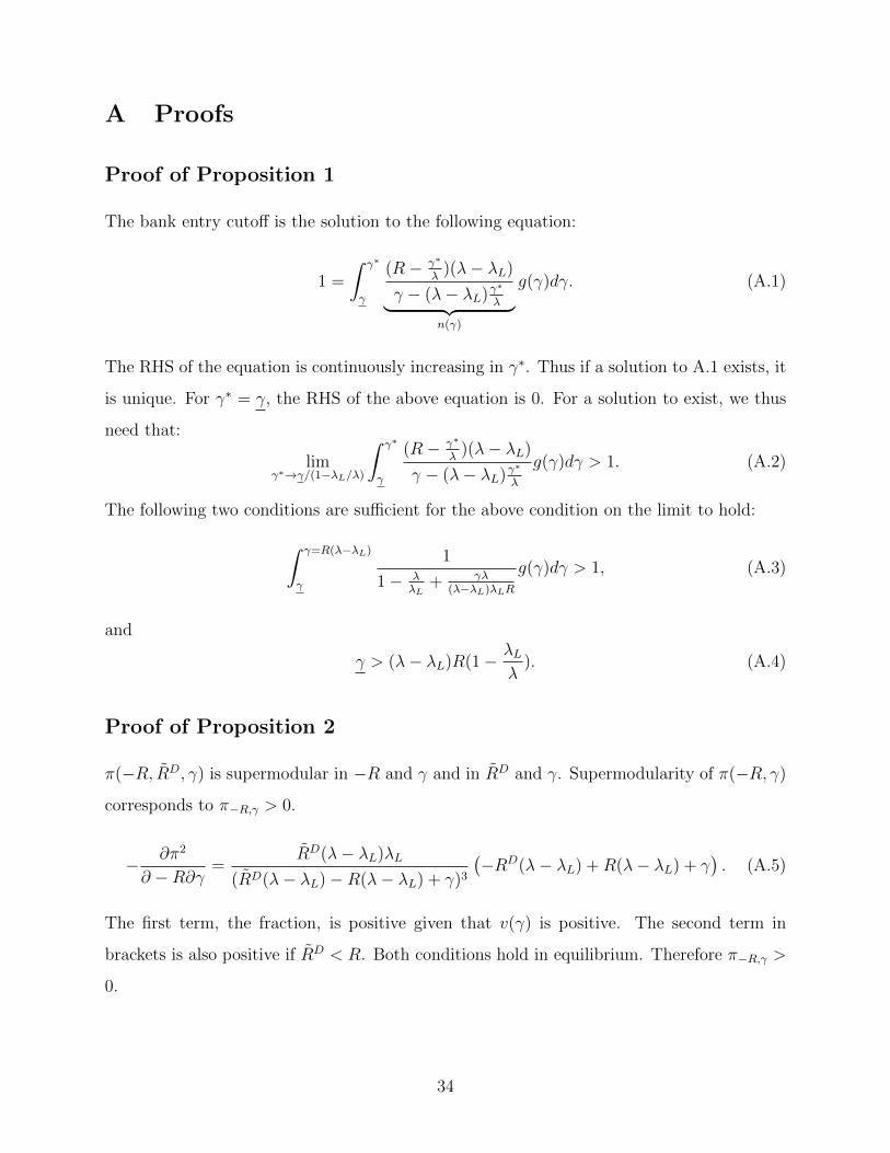
A Proofs

Proof of Proposition 1

The bank entry cutoff is the solution to the following equation:

1 =

∫ γ∗

γ

(R− γ∗

λ)(λ− λL)

γ − (λ− λL)γ∗

λ︸ ︷︷ ︸n(γ)

g(γ)dγ. (A.1)

The RHS of the equation is continuously increasing in γ∗. Thus if a solution to A.1 exists, it

is unique. For γ∗ = γ, the RHS of the above equation is 0. For a solution to exist, we thus

need that:

limγ∗→γ/(1−λL/λ)

∫ γ∗

γ

(R− γ∗

λ)(λ− λL)

γ − (λ− λL)γ∗

λ

g(γ)dγ > 1. (A.2)

The following two conditions are sufficient for the above condition on the limit to hold:

∫ γ=R(λ−λL)

γ

1

1− λλL

+ γλ(λ−λL)λLR

g(γ)dγ > 1, (A.3)

and

γ > (λ− λL)R(1− λLλ

). (A.4)

Proof of Proposition 2

π(−R, RD, γ) is supermodular in −R and γ and in RD and γ. Supermodularity of π(−R, γ)

corresponds to π−R,γ > 0.

− ∂π2

∂ −R∂γ=

RD(λ− λL)λL

(RD(λ− λL)−R(λ− λL) + γ)3

(−RD(λ− λL) +R(λ− λL) + γ

). (A.5)

The first term, the fraction, is positive given that v(γ) is positive. The second term in

brackets is also positive if RD < R. Both conditions hold in equilibrium. Therefore π−R,γ >

0.

34

Supermodularity of π(RD, γ) corresponds to πRD,γ > 0.

− ∂π2

∂RD∂γ=

λL(λ− λL)

(RD(λ− λL)−R(λ− λL) + γ)3

((R(λ− λL)− γ)(R− RD) + γRD

). (A.6)

The first term, the fraction, is positive given that v(γ) is positive. The second term in

brackets is also positive if RD < R and R(λ − λL) − γ > 0. The three conditions hold in

equilibrium. Therefore πRD,γ > 0.

Assume Rj < Ri. Supermodularity of π(−R, γ) implies that for any two bankers of type

γ1 and γ2 < γ1:

π(Rj, γ1)− π(Rj, γ2) > π(Ri, γ1)− π(Ri, γ2) (A.7)

⇒ π(Ri, γ2)− π(Rj, γ2) > π(Ri, γ1)− π(Rj, γ1) (A.8)

⇒ π(Ri, γ2)− fLij − π(Rj, γ2) > π(Ri, γ1)− fLij − π(Rj, γ1) (A.9)

⇒ πXij (γ2)− πXjj(γ2) > πXij (γ1)− πXjj(γ1). (A.10)

This relationship holds for any pair of bankers. Let γLj denote the banker who is indifferent

between investing at home and abroad. If some bankers invest abroad while others invest

only at home, then this implies that all bankers of type γj ≤ γLj invest abroad while all

bankers for whom γj > γLj invest at home. The logic is analogous for cross-border borrowing

and operations through foreign affiliates.

Proof of Proposition 3

The uniqueness of an interior equilibrium is proven as follows. It is shown that equation 21

can be expressed only as a function of γ∗h so that the RHS of the equation is continuously

increasing in γ∗h. Under the sufficient condition that

limγ∗h→γh/(1−λL/λ)

∫ γ∗h

γh

(R− γ∗hλ

)(λ− λL)

γh − (λ− λL)γ∗hλ

g(γh)dγh > 1, (A.11)

the RHS cuts the LHS of the equation once.

35

Consider again equation 21:

Kh = Kh

∫ max{γFh ,γBh }

γh

gh(γh)dγh +Kh

∫ γ∗h

max{γFh ,γBh }n(γh, R,R

Dh )gh(γh)dγh (A.12)

From equations 22 and 23, RDf = R−γ∗1/λ andRD

h = R−γ∗h/λ. Therefore ∂n(γh, R,RDh )/∂γ∗h >

0. Because n(γh, R,RDh ) > 1, the RHS of equation 21 increase in γ∗h if:

dmax{γFh , γBh }dγ∗h

=∂max{γFh , γBh }

∂γ∗h+∂max{γFh , γBh }

∂γ∗f

dγ∗fdγ∗h

< 0. (A.13)

Note that equations 24 and 25 give unique solutions to the cutoffs γBh and γAh for permissible

parameter values. The following partial derivatives are easy to derive using implicit function

theorems: ∂γB

∂γ∗h< 0, ∂γB

∂γ∗f> 0, ∂γA

∂γ∗f> 0, ∂γA

∂γ∗h≤ 0. Now consider again equation 20:

Kf = Kf

∫ γ∗f

γf

n(γf , R,RDf )gf (γf )dγf +D

with

D = Kh

∫ max{γh,γFh }

γh

(n(γh, R,RDf )− 1)gh(γh)dγh (A.14)

+ Kh

∫ max{γFh ,γBh }

max{γh,γFh }

(n(γh, R, φRDf )− 1)gh(γh)dγh. (A.15)

This equation implicitly gives γ∗f (γ∗h) and implies:

dγ∗fdγ∗h

=∂γ∗f∂D

dD

dγ∗h, (A.16)

where∂γ∗f∂D

< 0.dD

dγ∗h=∂D

∂γ∗h+∂D

∂γ∗f

dγ∗fdγ∗h

. (A.17)

Because∂γBh∂γ∗h

< 0,∂γAh∂γ∗h

< 0 and n(γh, R,RDf ) > n(γh, R, φR

Df ), it follows that ∂D

∂γ∗h< 0. Also,

∂D∂γ∗f

> 0.

dDdγ∗h

must then be negative by contradiction. Suppose dDdγ∗h

was positive. This would

36

imply thatdγ∗fdγ∗h

was negative. Plugging this expression into equation A.17 would result in

dDdγ∗h

< 0, which is a contradiction. If dDdγ∗h

< 0, it follows that dEdγ∗h

< 0. This implies that

dmax{γFh ,γBh }

dγ∗h< 0.

Proof of Comparative Statics Results

I derive comparative statics locally for the case where γh< γAh < γBh < γ∗h.

Proof of Proposition 4 To showdγBhdKf

> 0,dγAhdKf

> 0 andddfhdKf

> 0.

Note that Kf only enters equation 20. Therefore, dDdKf

> 0. D can only increase with

an increase in Kf if a bigger mass of home bankers borrow from depositors in the foreign

country. This is only possible if the equilibrium difference between γ∗f and γ∗h is bigger. As

a result, γBh and γAh must increase. More formally:

SupposedγBhdKf

< 0. This would imply thatd(γ∗f−γ

∗h)

dKf< 0 and hence, dD

dKf< 0. But if

dDdKf

< 0, then, from equation 20,dγAhdKf

> 0, which is a contradiction.

SupposedγAhdKf

< 0. This would imply thatd(γ∗f−γ

∗h)

dKf< 0 and hence, dD

dKf< 0. But if

dDdKf

< 0, then, from equation 20,dγBhdKf

> 0, which is a contradiction.

With a larger equilibrium gap in ∆γ∗ = γ∗f − γ∗h, the volume of borrowing dfh =

n(γh, R, φRDf )− 1 must go up.

Proof of Proposition 5 To showdγBhd∆

> 0,dγAhd∆

> 0 andddfhd∆

> 0.

An increase in ∆ increases γ∗f ceteris paribus. A higher γ∗f implies that γBh and γAh

increase and thus the equilibrium gap ∆γ∗ = γ∗f − γ∗h is higher. So the volume of borrowing

d12 = n(γh, R, φRDf )− 1 goes up. More formally:

SupposedγBhd∆

< 0. This would imply thatd(γ∗f−γ

∗h)

dKf< 0 and hence, dD

dKf< 0. But if

dDdKf

< 0, then from equation 20dγBhd∆

> 0, which is a contradiction.

SupposedγAhd∆

< 0. This would imply thatd(γ∗f−γ

∗h)

dKf< 0 and hence, dD

dKf< 0. But if

dDdKf

< 0, then from equation 20dγBhd∆

> 0, which is a contradiction.

With a larger equilibrium gap in ∆γ∗ = γ∗f − γ∗h, the volume of borrowing dfh =

n(γh, R, φRDf )− 1 must go up.

37

Proof of Proposition 6 To showdγBhdφ

< 0 anddγAhdφ

> 0. SupposedγBhdφ

> 0. This would

required(γ∗f−γ

∗h)

dφ> 0. But if

d(γ∗f−γ∗h)

dφ> 0, from equation 21,

dγ∗hdφ

> 0 and becausedγAhdφ

> 0,

from equation 20,dγ∗fdφ

< 0, which contradictsd(γ∗f−γ

∗h)

dφ> 0.

The proofs of the comparative statics with respect to fA and fB follow equivalently.

38

B General Model with τ = φ = 1

In this appendix, I characterize the solution to the general model. I discuss the different

equilibrium cases that can occur for various parameter values and provide intuition for how

the equilibrium case changes with key parameters of the model. To reduce the dimensionality,

I assume that there are no variable costs to operating cross-border, i.e. τ = φ = 1. This

removes the decision of firms between operating from home or through FDI.

The following equilibrium cases can occur (corner solutions where all capitalists become

depositors or bankers in one of the two countries are not considered):54

Proposition 7 Assume φ = τ = 1. Then the following equilibrium cases are conceivable

where i, j ∈ {1, 2} and i 6= j:

(i) No trade.

(ii) Cross-border lending by banking sector j: Some banks from country j invest

domestic deposits in country i. γLj exists.

(iii) Cross-border lending and local intermediation by banking sector j: Some

banks from country j invest domestic deposits in country i; others raise foreign deposits and

invest them in the foreign market. γLj and γBj both exist.

(iv) Local intermediation by banking sector j: Some banks from country j raise foreign

deposits and invest them in the foreign market. γBj exists and Ri > Rj.

(v) Local intermediation and cross-border borrowing by banking sector j: Some

banks from country j raise deposits in country i and invest them at home and abroad. γBj

exists and Ri = Rj.

(vi) Cross-border lending by banking sector j and cross-border borrowing by

banking sector i: Some banks from country j invest domestic deposits abroad, while some

banks from country i raise deposits in country j and invest them at home. γLj and γBi both

exist.

(vii) Cross-border borrowing by banking sector i: Some banks from country i raise

deposits in country j and invest them at home. γBi exists and Ri > Rj.

54The word exist in the following means that the indifference condition that determines the respectivecutoff has a solution and that this solution lies in the range of permissible values. For example, the cutoffγLi exists if it solves π(γj) = πXij (γj) and γLi ∈ {γj , γ

∗j}.

39

Proof. Assume Ai = Aj and ∆(K/L) =Kj

Lj− Ki

Li≥ 0 without loss of generality.

(a) ∆(K/L) ≥ 0 implies that in equilibrium Ri ≥ Rj. To see this note that if Ri > Rj in

autarky, it must be the case that Ri ≥ Ri in equilibrium. It is possible that banks source

so much foreign capital from abroad for investment at home that rates of return to capital

equalize in equilibrium. If Ri = Rj in autarky, then in equilibrium Ri = Rj. This leaves the

following combinations of equilibrium gross returns to capital and deposit rates possible:

(1) Ri > Rj & RDi < RD

j

(2) Ri > Rj & RDi > RD

j

(3) Ri > Rj & RDi = RD

j

(4) Ri = Rj & RDi < RD

j

(5) Ri = Rj & RDi > RD

j

(6) Ri = Rj & RDi = RD

j

(b) There are no upper limits on fLij , fLji, f

Bij and fBji . So any of these fixed costs can be

prohibitively high.

(c) In each country j ∈ {1, 2}, there are four possibilities: γLj and γBj both do not exist ,

only γLj exists, only γBj exists, both γLj and γBj exist.

(d) Investing at home is costless in any case. Therefore if Ri > Rj, all banks in country i

must invest in country i.

(e) Capital must always flow in one direction, i.e. it cannot be the case that banks from

country j invest in country i and banks from country i invest in j.

(f) If Ri = Rj, no banker incurs the fixed cost of cross-border lending in equilibrium.

(g) It is not possible that banks in both countries raise deposits abroad in equilibrium. If

RDi > RD

j only banks in country i have incentives to invest in the fixed cost of FDI.

(h) If RDi = RD

j , no banker incurs the fixed cost of cross-border borrowing in equilibrium.

Combining (a)-(h), we have that:

(1) If Ri > Rj & RDi < RD

j , γLi does not exist and γBi does not exist.

(2) If Ri > Rj & RDi > RD

j , γLi does not exist and γBi does not exist. Banks in country i all

invest in country i.

(3) If Ri > Rj & RDi = RD

j , γLi does not exist and γBi and γBj do not exist.

(4) If Ri = Rj & RDi > RD

j , γLi , γLj and γBj do not exist. Banks in both countries are

40

indifferent where to invest.

(5) If Ri = Rj & RDi < RD

j , γLi , γLj and γBi do not exist. Banks in both countries are

indifferent where to invest.

(6) If Ri = Rj & RDi = RD

j , γLi , γLj , γBi and γBj do not exist. The equilibrium corresponds

to autarky.

Therefore, it can be that:

(A) There is no trade. Possible in all cases.

(B) Only γLj exists. Possible for cases (1) and (2).

(C) γLj and γBj both exist: Possible for case (1).

(D) γLj and γBi both exist: Possible for case (2).

(E) γBj exists: Possible for case (1) and (5).

(F) γBi exists: Possible for case (2) and (4).

Now distinguish (E) and (F) again by the equilibrium values that Ri and Rj take:

(E1) γBj exists and (1): banks that pay fBij invest in country i.

(E2) γBj exists and (5): banks in country j invest at home and abroad.

(F1) γBi exists and (2): banks that pay fBji invest in country i.

(F2) γBi exists and (4): banks in country i invest at home and abroad.

Then, we obtain the eight cases as stated in the proposition.

Figure B.1, which is obtained from simulating the model numerically, illustrates the

different equilibrium cases. It shows how the equilibrium changes with the capital-labor

ratio of country 1 K1/L1 and with the support of the monitoring cost distribution of country

1, i.e. with changes in γ1

keeping the characteristics of country 2 fixed. As the size of

the capital stock affects the realized monitoring cost distribution, the capital-labor ratio of

country 1 is varied by modifying the labor endowment instead of the capital endowment and

A1 = A2.

Consider figure B.1 and focus on the case where country 1 is relatively capital scarce.

Start from a situation where country 1 has a very efficient banking sector relative to country 2,

i.e. begin in the right lower corner of the graph. Under the assumed parameters, equilibrium

case (vii) prevails, that is, banking sector 1 borrows capital from depositors in country 2

41

for investment at home, hence importing capital from country 2. Banking sector 2 operates

only at home.

Figure B.1: Equilibrium types as a function of K1/L1 and γ1

iii) Local intermediation and cross-

border lending 2

vi) Cross-border lending 2, cross-

border borrowing 1

γ1

K2/L

2 -K

1/L

1

viii) Local intermediation and

cross-border borrowing 1,

R1=R

2

vii) Cross-border borrowing 1

ii) Cross-border lending 2i) �o trade

iv) Local

intermediation 2

v) Local intermediation and

cross-border borrowing 2,

R1=R

2

The graph is obtained from simulating the model for the following parameter values:Cobb-Douglas production function with a labor share of 0.3, λL = 0.5, λ = 0.985, fL =0.13, fB = 0.16, uniform distribution, γ

2= 0.04 and γ1 = γ2 = 0.4, K2/L2 = 20/3,

A1 = A2, K1/L1 ∈ [20/3, 20/4.5], γ1∈ [0.035, 0.05].

Next move upward along the y-axis. As γ1

increases and banking sector 1 becomes less

efficient, banks in country 2 start to engage in cross-border lending simultaneously (case (vi)).

Because the interest rate in country 1 decreases and because banks in country 1 become less

efficient, fewer banks in country 1 borrow from depositors abroad. This implies that the

spread in gross returns to capital grows larger ceteris paribus, which makes it attractive for

banks in country 2 to invest abroad.

As the efficiency of banking sector 1 decreases even more, banks in country 1 are, at some

42

point, not efficient enough and differences in deposit rates are not large enough to make any

bank in country 1 incur the fixed cost of cross-border borrowing. In this case, only banking

sector 2 is active across borders and lends to firms in country 1 (case (ii)).

With a further decline in γ1, the deposit rate in country 1 can decrease to the point

where it is profitable for banks in country 2 not only to lend to firms in country 1 but also to

borrow from depositors in country 1. Then, banking sector 2 engages in both cross-border

lending and borrowing in equilibrium, exporting capital on net (case (iii)).

Next, consider how the equilibrium varies along the x-axis, that is, with changes in

K1/L1. Start where countries have equal capital endowments so that there is no reason why

capital should flow across borders. If differences in efficiencies are also small (γi ≈ 0.04),

there is no trade in banking services at all. The equilibrium corresponds to autarky. If,

however, one banking sector is sufficiently more efficient than the other, that banking sector

expands by intermediating foreign deposits locally. With equal gross returns to capital in

the two countries, banks incur the fixed cost of cross-border borrowing and invest at home

and abroad to keep returns equated. This is the case discussed in section 4. Which banks

lend to firms at home and abroad, is not determined in this case. Because gross returns to

capital are equal, all banks that pay the fixed cost are indifferent between investing at home

and abroad.

Now let country 1 become capital scarce, that is, move to the right along the x-axis. As

the capital-labor ratio of country 1 declines, additional banks become internationally active.

Whether these are banks in country 1 or in country 2 depends on which banking sector is

more efficient. In a nutshell: differences in capital-labor ratios determine the direction of the

cross-border capital flow. Differences in banking sector efficiencies fix which banks channel

capital across borders. This intuition is similar to the model with homogenous banks in

Niepmann (2015).

43

C Data Appendix

External Position of Banks (AUSTA - “Auslandsstatus der Banken”): Total cross-

borders assets and liabilities of bank k in country i are measured as the cross-border assets

and liabilities of parent bank k minus the liabilities of its affiliates located in country i vis-

a-vis the parent. Local assets (liabilities) comprise the assets (liabilities) of all affiliates of

bank k located in country i towards residents of country i. Branches and subsidiaries are

matched to the parent as of June 2005. Data come at a monthly frequency and are averaged

over 12 months. See Fiorentino et al. (2010) for a detailed description of the data source.

Monthly Balance Sheet Statistics (BISTA - “Monatliche Bilanzstatistik”) and

Income and Loss Data (GuV - “Gewinn und Verlustrechnung der Banken”):

Information on balance sheet size, bank equity, overhead costs and the number of employees

are from Monthly balance sheet statistics and Income and loss data available at the Deutsche

Bundesbank. Values represent yearly averages for the parent bank plus its domestic and

foreign branches.

Data on marginal products of capital (MPK): David et al. (2014) kindly provided

information on capital stocks and MPKs by country. The MPKs used in this paper are

based on the method suggested by Caselli and Feyrer (2007) and were calculated using

country specific prices of output, consumption and investment. I complement the dataset

with information on the labor force. I then assume a Cobb-Douglas production function

Y = AKαL1−α with a capital share of α = 0.3 consistent with David et al. (2014) to back

out A for the simulation and normalize the Czech Republic’s capital stock by the German

capital stock. The regressions include MPK values for the year 2000.

Additional variables: GDP in current $US and GDP per capita in current $US are ob-

tained from the World Development Indicators. Data on average overhead costs to total

assets of a country are from the World Bank’s Financial Development and Structure Dataset

(see Beck et al. (2009)). Distance to Germany comes from a dataset provided by CEPII (see

Mayer and Zignago (2005)). The Financial Freedom Index is from the Heritage Foundation.

Bureaucratic quality is from the International Country Risk Guide provided by the PRS

Group.

44

References

Adrian, Tobias and Hyun Song Shin, “Procyclical Leverage and Value-at-Risk,” Review

of Financial Studies, 2014, 27 (2), 373–403.

Allen, Franklin, Thorsten Beck, Elena Carletti, Philip R. Lane, Dirk Schoen-

maker, and Wolf Wagner, “Cross-Border Banking in Europe: Implications for Finan-

cial Stability and Macroeconomic Policy,” Technical Report, Center for Economic Policy

Research June 2011.

Antras, Pol and Ricardo J. Caballero, “Trade and Capital Flows: A Financial Frictions

Perspective,” Journal of Political Economy, 08 2009, 117 (4), 701–744.

Beck, Thorsten, Asli Demirguc-Kunt, and Ross Levine, “Bank concentration, com-

petition, and crises: First results,” Journal of Banking & Finance, May 2006, 30 (5),

1581–1603.

, Asli Demirguc-Kunt, and Ross Levine, “Financial institutions and markets across

countries and over time - data and analysis,” Policy Research Working Paper Series 4943,

The World Bank May 2009.

Berger, Allen N. and Loretta J. Mester, “Inside the black box: What explains differ-

ences in the efficiencies of financial institutions?,” Journal of Banking & Finance, 1997,

21 (7), 895 – 947.

Bernard, Andrew B., J. Bradford Jensen, Stephen J. Redding, and Peter K.

Schott, “The Empirics of Firm Heterogeneity and International Trade,” Annual Review

of Economics, 2012, 4 (1), null.

, Jonathan Eaton, J. Bradford Jensen, and Samuel Kortum, “Plants and Pro-

ductivity in International Trade,” American Economic Review, September 2003, 93 (4),

1268–1290.

Blas, Beatriz De and Katheryn Russ, “FDI in the Banking Sector,” NBER Working

Papers 16029, National Bureau of Economic Research 2010.

45

and , “All banks great, small, and global: Loan pricing and foreign competition,”

International Review of Economics and Finance, 2012. Forthcoming.

Brevoort, Kenneth P and John D Wolken, “Does distance matter in banking?,” The

Changing Geography of Banking and Finance, 2009, pp. 27–56.

Buch, Claudia M., “Information or Regulation: What Drives the International Activities

of Commercial Banks,” Journal of Money Credit and Banking, 2003, 35 (6), 851–869.

, “Distance and International Banking,” Review of International Economics, 2005, 13 (4),

787–804.

, Catherine Tahmee Koch, and Michael Koetter, “Size, productivity and interna-

tional banking,” Journal of International Economics, 2011, 85 (2), 329–334.

, , and , “Should I stay or should I go? Bank productivity and internationalization

decisions,” Journal of Banking & Finance, 2014, 42, 266 – 282.

Caselli, Francesco and James Feyrer, “The Marginal Product of Capital,” The Quarterly

Journal of Economics, 2007, 122 (2), 535–568.

Committee on the Global Financial System, “Long-term issues in international bank-

ing,” CGFS Paper 41, Bank for International Settlements July 2010.

Corbae, Dean and Pablo D’Erasmo, “A Quantitative Model of Banking Industry Dy-

namics,” 2010 Meeting Papers 268, Society for Economic Dynamics 2010.

and , “Foreign Competition and Banking Industry Dynamics: An Application to

Mexico,” IMF Economic Review. Forthcoming.

David, Joel M., Espen Henriksen, and Ina Simonovska, “The Risky Capital of Emerg-

ing Markets,” NBER Working Papers 20769, National Bureau of Economic Research, Inc

December 2014.

Degryse, Hans and Steven Ongena, “Distance, Lending Relationships, and Competi-

tion,” The Journal of Finance, 2005, 60 (1), 231–266.

46

Detragiache, Enrica, Abdul Abiad, and Thierry Tressel, “A New Database of Fi-

nancial Reforms,” IMF Working Papers 08/266, International Monetary Fund 2008.

Ennis, Huberto M., “On the size distribution of banks,” Economic Quarterly, 2001, Fall,

1–25.

Fillat, Jose L, Stefania Garetto, and Martin Gotz, “Multinational Banks,” Technical

Report 2015. Mimeo.

Fiorentino, Elisabetta, Catherine Koch, and Winfried Rudek, “External Position

Reports of German Banks - A Description of the Microdatabase,” Technical Documenta-

tion, Deutsche Bundesbank 2010.

Focarelli, Dario and Alberto F. Pozzolo, “Where Do Banks Expand Abroad? An

Empirical Analysis,” Journal of Business, November 2005, 78 (6), 2435–2464.

Francois, Joseph and Bernard Hoekman, “Services Trade and Policy,” Journal of

Economic Literature, 2010, 48 (3), 642–92.

Helpman, Elhanan, Marc J. Melitz, and Stephen R. Yeaple, “Export Versus FDI

with Heterogeneous Firms,” American Economic Review, 2004, 94 (1), 300–316.

Holmstrom, Bengt and Jean Tirole, “Financial Intermediation, Loanable Funds, and

the Real Sector,” The Quarterly Journal of Economics, August 1997, 112 (3), 663–91.

Hughes, Joseph P. and Loretta J. Mester, “Efficiency in banking: theory, practice,

and evidence,” Technical Report 2008.

Janicki, Hubert P. and Edward Simpson Prescott, “Changes in the size distribution

of U.S. banks: 1960-2005,” Economic Quarterly, 2006, (Fall), 291–316.

Ju, Jiandong and Shang-Jin Wei, “Domestic Institutions and the Bypass Effect of

Financial Globalization,” American Economic Journal: Economic Policy, 2010, 2 (4),

173–204.

Kalemli-Ozcan, Sebnem, Bent Sorensen, and Sevcan Yesiltas, “Leverage across

firms, banks, and countries,” Journal of International Economics, 2012, 88 (2), 284 – 298.

47

Kerl, Cornelia and Friederike Niepmann, “What determines the composition of inter-

national bank flows?,” IMF Economic Review. Forthcoming.

Lehner, Maria, “Entry mode choice of multinational banks,” Journal of Banking and

Finance, 2009, 33, 1781–1792.

Mayer, Thierry and Soledad Zignago, “Market Access in Global and Regional Trade,”

Working Papers 2005-02, CEPII research center January 2005.

McCord, Roisin, Edward Simpson Prescott et al., “The Financial Crisis, the Collapse

of Bank Entry, and Changes in the Size Distribution of Banks,” Economic Quarterly, 2014,

(1Q), 23–50.

Melitz, Marc J., “The Impact of Trade on Intra-Industry Reallocations and Aggregate

Industry Productivity,” Econometrica, November 2003, 71 (6), 1695–1725.

Mrazova, Monika and J. Peter Neary, “Selection effects with heterogeneous firms,”

Economics Series Working Papers 588, University of Oxford, Department of Economics

2011.

Niepmann, Friederike, “Banking across borders with heterogeneous banks,” FRB of New

York Staff Report, 2013, (609).

, “Banking across borders,” Journal of International Economics, 2015, 96 (2), 244 – 265.

Papaioannou, Elias, “What drives international financial flows? Politics, institutions and

other determinants,” Journal of Development Economics, March 2009, 88 (2), 269–281.

Yeaple, Stephen R., “Firm heterogeneity and the structure of U.S. multinational activity,”

Journal of International Economics, July 2009, 78 (2), 206–215.

48

Tables

Table 1: Parameters used to simulate the model

Exogeneous parameters ValuesSize of capital input per firm z 1Capital share α in Cobb-Douglas production function 0.3Shape parameter of Pareto distribution 0.55Lower bound of Pareto distribution GER γG 0.006317

Lower bound of Pareto distribution CZE γC 0.010344

Capital endowment GER KG 1Labor endowment GER LG 5.61TFP GER AG 0.064524Capital endowment CZE KC 0.08145Capital endowment CZE LC 0.72206TFP CZE AC 0.046366Success probability without monitoring λL 0.85Success probability with monitoring λ 0.9Variable cost of borrowing abroad φ 1.001Fixed cost of borrowing abroad fB 0.24

The table summarizes the parameter values that are used to simulate the model.See section 4.2 for details.

49

Table

2:

Outc

omes

ofth

em

odel

sim

ula

tion

Clo

sed

Eco

nom

yB

ase

lin

eH

et.

IH

et.

II(1

)(2

)(3

)(4

)(5

)(6

)(7

)(8

)(9

)M

omen

tsB

ase

line

Het

1H

et2

Base

lin

eC

han

ge

Het

1C

han

ge

Het

2C

han

ge

Dep

osit

rate

GE

RRD G

1.0

558

1.0

558

1.0

560

1.0

556

-0.0

17%

1.0

556

-0.0

13%

1.0

559

-0.0

13%

Dep

osit

rate

CZ

ERD C

1.0

457

1.0

513

0.5

36%

1.0

511

0.5

17%

1.0

515

0.5

52%

Gro

ssre

turn

toca

pit

alG

ERRG

1.0

647

1.0

647

-0.0

05%

1.0

647

-0.0

05%

1.0

647

-0.0

05%

Gro

ssre

turn

toca

pit

alC

ZERC

1.0

641

1.0

647

0.0

57%

1.0

647

0.0

57%

1.0

647

0.0

57%

Sh

are

ofb

anke

rsG

ER

0.1

260

0.1

303

0.1

266

0.1

328

5.3

73%

0.1

367

4.9

06%

0.1

335

5.4

64%

Sh

are

ofb

anke

rsC

ZE

0.2

275

0.0

800

-64.8

16%

0.0

876

-61.4

73%

0.0

736

-67.6

62%

Ave

rage

bal

ance

shee

tsi

zeG

ER

7.9

359

7.6

765

7.9

008

7.8

981

-0.4

77%

7.6

529

-0.3

07%

7.8

749

-0.3

28%

Ave

rage

bal

ance

shee

tsi

zeC

ZE

4.3

959

8.2

531

87.7

45%

9.5

380

116.9

75%

7.2

605

65.1

64%

Ave

rage

mon

itor

ing

cost

GE

R0.0

071

0.0

073

0.0

071

0.0

072

0.7

06%

0.0

074

0.4

85%

0.0

072

0.5

23%

Ave

rage

mon

itor

ing

cost

sC

ZE

0.0

131

0.0

112

-14.6

13%

0.0

112

-13.9

68%

0.0

111

-15.1

55%

Top

10co

nce

ntr

atio

nG

ER

0.1

120

0.1

090

0.1

087

0.1

138

1.6

39%

0.1

105

1.4

32%

0.1

104

1.5

77%

Top

10co

nce

ntr

atio

nC

ZE

0.1

234

0.1

073

-12.9

87%

0.1

081

-12.3

86%

0.1

067

-13.4

94%

Net

inte

rest

mar

gin

GE

RRG−RD G

0.0

090

0.0

090

0.0

087

0.0

091

1.4

24%

0.0

091

0.9

88%

0.0

088

1.0

66%

Net

inte

rest

mar

gin

CZ

ERC−RD C

0.0

184

0.0

134

-27.2

11%

0.0

136

-26.1

04%

0.0

132

-28.1

33%

Ban

kin

gse

ctor

pro

fits

GE

R0.1

207

0.1

245

0.1

210

0.1

272

5.4

11%

0.1

307

4.9

29%

0.1

276

5.4

90%

Ban

kin

gse

ctor

pro

fits

CZ

E0.2

178

0.0

761

-65.0

66%

0.0

834

-61.7

34%

0.0

699

-67.9

%R

etu

rnto

wor

kers

GE

R5.1

8494

5.1

8498

0.0

01%

5.1

8498

0.0

01%

5.1

8498

0.0

01%

Ret

urn

tow

orke

rsC

ZE

0.6

6081

0.6

6077

-0.0

07%

0.6

6077

-0.0

07%

0.6

6077

-0.0

07%

Dep

osit

sp

aid

GE

R0.8

3046

0.8

264

0.8

301

0.8

2389

-0.7

91%

0.8

2023

0.0

00%

0.8

2346

-0.8

05%

Dep

osit

sp

aid

CZ

E0.7

2704

0.8

7045

19.7

25%

0.8

6308

18.7

12%

0.8

7671

20.5

87%

Wel

fare

(nor

m.)

GE

R1

1.0

0000

0.0

00%

1.0

0000

0.0

00%

1.0

0000

0.0

00%

Wel

fare

(nor

m.)

CZ

E1

1.0

0013

0.0

13%

1.0

0011

0.0

11%

1.0

0014

0.0

14%

Glo

bal

(nor

m.)

Wel

fare

11.0

0001

0.0

01%

1.0

0001

0.0

01%

1.0

0002

0.0

02%

Cro

ss-b

ord

erb

orro

win

gcu

toffγB

0.0

064

0.0

068

0.0

066

Fra

ctio

nof

Ger

man

ban

ks

acti

vein

CZ

E0.0

449

0.0

440

0.0

489

Sh

are

ofG

erm

anlo

ans

into

tal

Cze

chcr

edit

0.5

926

0.5

569

0.6

234

Sh

are

ofG

erm

anas

sets

hel

din

CZ

E0.0

454

0.0

428

0.0

477

Equ

ity

exp

ort

ofG

erm

anb

anks

0.0

060

0.0

060

0.0

065

Th

eta

ble

show

sth

eou

tcom

esof

the

mod

elsi

mu

lati

on

.C

olu

mn

s(1

)to

(3)

pre

sent

the

equ

ilib

riu

mva

lues

of

vari

ou

sva

riab

les

inth

ecl

ose

dec

on

om

y.C

olu

mn

(1)

show

seq

uil

ibri

um

valu

esfo

rth

eb

ase

lin

ecl

ose

dec

on

om

yd

escr

ibed

inta

ble

1,

colu

mn

(2)

for

the

close

dec

on

om

yw

ith

aP

are

tosh

ap

ep

aram

eter

ofa

=0.

75an

da

low

erli

mit

ofγG

=0.

0065267,

and

colu

mn

(3)

for

the

close

dec

on

om

yw

itha

=0.

75

an

dγG

=0.

0066995.

Bla

nk

space

sin

colu

mn

s(2

)an

d(3

)in

dic

ate

that

valu

esar

eth

esa

me

as

those

inco

lum

n(1

)fo

rth

eb

ase

lin

ecl

ose

dec

on

om

y.C

olu

mn

(4)

dis

pla

ys

mod

elou

tcom

esfo

rth

eb

asel

ine

open

econ

omy.

Col

um

n(5

)gi

ves

the

chan

ges

inp

erce

nt

com

pare

dto

the

close

dec

on

om

y.

Colu

mn

(6)

an

d(8

)su

mm

ari

zeth

eop

enec

onom

you

tcom

esw

hen

the

deg

ree

ofh

eter

ogen

eity

of

the

Ger

man

bankin

gse

ctor

isch

an

ged

.In

colu

mn

(6),a

=0.7

5an

dγG

=0.0

066995.

Inco

lum

n(8

),a

=0.7

5an

dγG

=0.0

0652

67.

Colu

mns

(7)

an

d(9

)giv

eth

eco

rres

pon

din

gch

an

ges

inou

tcom

esin

per

cent

com

pare

dto

the

resp

ecti

vecl

osed

econ

omy

case

.

50

Table 3: Relationship between bank size, leverage and efficiency

log(size)k(1) (2)

log(equityk) 1.003*** 1.012***(0.00898) (0.00781)

log(overhead costsk) -0.287***(0.0477)

log(labor prod.k) 0.194***(0.0350)

Constant 10.68*** 8.127***(0.173) (0.276)

Observations 1,909 1,909R2 0.960 0.957

The table presents results from regressing the log balance sheet size of bank k on its log equity andits efficiency. In column (1), a bank’s ratio of overhead costs to total assets is used as an inversemeasure of efficiency. Column (2) includes the bank’s number of assets per employee instead. Thesample comprises 1,909 German banks in 2005. Robust standard errors are in parentheses. ***p<0.01, ** p<0.05, * p<0.1. Data source: Research Data and Service Centre of the DeutscheBundesbank, External Position of Banks, Monthly Balance Sheet Statistics and Income and LossData.

Table 4: Effect of size and efficiency on the extensive and intensive margins

Extensive Margin: Logit Model Intensive Margin: OLS

cr. asski cr. liabki FDIki cr. asski local asski cr. liabki local liabki(1) (2) (3) (4) (5) (6) (7)

log(overheadk) -0.807*** -0.850*** -0.922*** -1.682*** -0.386 -1.347*** 0.00515(0.135) (0.126) (0.253) (0.232) (0.390) (0.232) (0.889)

Observations 337,705 339,624 110,606 35758 251 59259 241(Pseudo) R2 0.483 0.375 0.458 0.408 0.571 0.271 0.476

The table shows that the extensive and intensive margins of banking across borders vary systematically withbank efficiency. Columns (1) to (3) show the results of logit regressions. Columns (4) to (7) are obtainedfrom OLS regressions. In each regression, the dependent variable is regressed on bank k’s ratio of overheadcosts to total assets, which measures inversely the bank’s efficiency. The dependent variable takes a valueof 1 if bank k has cross-border assets (column 1), cross-border liabilities (column 2) or affiliates (column 3)in country i. In columns (4) and (6), the dependent variable reflects the cross-border assets and liabilitiesin country i on the balance sheet of the parent bank, respectively, in logs. In columns (5) and (7), thelocal positions, that is, the assets and liabilities of the parent’s foreign affiliates in country i, are used asright-hand side variables, also in logs. Regressions include country-fixed effects and dummies for one ofnine bank types. Standard errors clustered by bank are in parentheses. *** p<0.01, ** p<0.05, * p<0.1.Data source: Research Data and Service Centre of the Deutsche Bundesbank, External Position of Banks,Monthly Balance Sheet Statistics and Income and Loss Data.

51

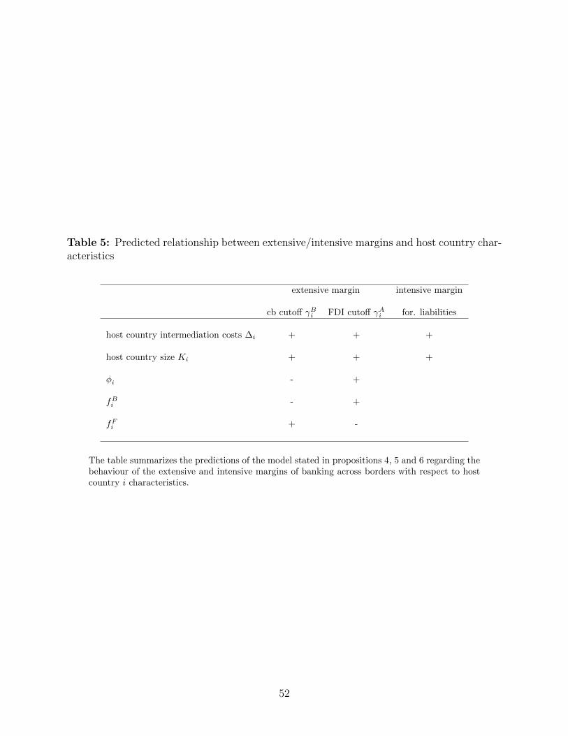
Table 5: Predicted relationship between extensive/intensive margins and host country char-acteristics

extensive margin intensive margin

cb cutoff γBi FDI cutoff γAi for. liabilities

host country intermediation costs ∆i + + +

host country size Ki + + +

φi - +

fBi - +

fFi + -

The table summarizes the predictions of the model stated in propositions 4, 5 and 6 regarding thebehaviour of the extensive and intensive margins of banking across borders with respect to hostcountry i characteristics.

52

Table 6: Relationship between extensive margin and host country characteristics

Extensive Margin: Logit Modelcr. assetski cr. liabilitieski FDIki

(1) (2) (3)log(overhead costsi) 0.473** 0.380** -0.208

(0.203) (0.193) (0.400)log(distance)i -0.483*** -0.444*** -0.781***

(0.137) (0.127) (0.161)fin. freedomi 0.0191* 0.0181*** 0.0187**

(0.00977) (0.00587) (0.00912)bureaucr. qualityi 0.551** 0.200 -0.0521

(0.227) (0.172) (0.304)log(GDP)i 0.739*** 0.844*** 0.954***

(0.0793) (0.0598) (0.148)log(GDP per cap.)i 0.244 -0.0254 -0.164

(0.169) (0.119) (0.204)MPKi 2.766** 0.687 -1.005

(1.288) (0.940) (2.584)

Observations 177,563 176,940 3,600Pseudo R2 0.5046 0.4511 0.4879

The table shows results from logit regressions. The dependent variable takes a value of 1 if bankk has cross-border assets (column 1), cross-border liabilities (column 2) or affiliates (column 3)in country i. The respective dependent variable is regressed on various country i characteristicsdescribed in detail in section 6.5. Regressions include bank-fixed effects. Standard errors clusteredby country are in parentheses. *** p<0.01, ** p<0.05, * p<0.1. Data source: Research Dataand Service Centre of the Deutsche Bundesbank, External Position of Banks. For details oncountry-level variables, see the data appendix.

53

Table 7: Cutoff regressions

cr. assets cr. liabilities FDImax. ovi average ovi max. ovi average ovi max. ovi average ovi

(1) (2) (3) (4) (5) (6)log(overhead costsi) 0.189* 0.0388** 0.324*** 0.0243*** 0.0398 0.0695

(0.0970) (0.0165) (0.0794) (0.00678) (0.0975) (0.0783)log(distance)i -0.229*** -0.0349*** -0.0949* -0.0117*** -0.248*** -0.0679*

(0.0642) (0.00944) (0.0493) (0.00402) (0.0451) (0.0386)fin. freedomi 0.00624** 0.00133** 0.00424* 0.000756*** -4.50e-05 -0.00165

(0.00239) (0.000543) (0.00244) (0.000234) (0.00321) (0.00318)bureaucr. qualityi 0.182** 0.0560*** 0.260*** 0.0141** -0.0310 0.0349

(0.0696) (0.0162) (0.0661) (0.00605) (0.0921) (0.0751)log(GDP)i 0.189*** 0.0322*** 0.257*** 0.0260*** -0.00834 -0.0448

(0.0406) (0.00802) (0.0306) (0.00265) (0.0312) (0.0292)log(GDP per cap.)i -0.0489 -0.0306** -0.0981** -0.00413 0.0617 -0.0766

(0.0408) (0.0118) (0.0449) (0.00540) (0.0578) (0.0550)MPKi -0.101 -0.115 -0.694 -0.0386 -0.217 0.218

(0.503) (0.114) (0.508) (0.0440) (1.514) (1.056)Constant 1.900* 2.679*** 0.0372 2.577*** 4.870*** 5.164***

(1.103) (0.186) (0.867) (0.0817) (0.910) (0.873)

Observations 96 96 97 97 38 38R-squared 0.623 0.512 0.647 0.724 0.629 0.247

The table demonstrate that there is strong sorting of banks into foreign activities based on host countrycharacteristics. In column 1, the dependent variable corresponds to the ratio of overhead costs to total assetsof the least efficient bank that has cross-border assets in country i. Accordingly, there is one observationper country in the underlying sample. In column 2, the dependent variable represents the average ratio ofoverhead costs to total assets of all banks that have cross-border assets in country i. In columns (3) and (4),maximum and average overhead costs are determined based on banks’ foreign liabilities. In columns (5) and(6), maximum and minimum overhead costs are taken over those banks that have one or more affiliates incountry i. In each column, the respective dependent variable is regressed on host country i characteristics.Robust standard errors are in parentheses. *** p<0.01, ** p<0.05, * p<0.1. Data source: Research Data andService Centre of the Deutsche Bundesbank, External Position of Banks, Monthly Balance Sheet Statisticsand Income and Loss Data. For details on country-level variables, see the data appendix.

54

Figures

Figure 1: Sorting of banks into cross-border lending, cross-border borrowing and FDI0

.02

.04

.06

.08

kern

el d

ensi

ty o

verh

ead

cost

s to

ass

ets

0 20 40 60 80

FDI Cr. LendingCr. Borrowing all

The figure illustrates that banks sort into foreign activities based on their efficiency proxied by a bank’sratio of overhead costs to total assets. Specifically, the chart plots the overhead costs distribution of differentgroups of German banks in 2005. The solid line shows the distribution for all banks in the bank-level datasetfrom the Deutsche Bundesbank. The dash-dotted line depicts the overhead cost distribution of banks withcross-border assets in country i. The line with long (short) dashes represents the size distribution of bankswith cross-border liabilities (affiliates) in country i. Source: Research Data and Service Centre of theDeutsche Bundesbank, External Position of Banks, Monthly Balance Sheet Statistics and Income and Lossdata, 2005, own calculations.

55

Figure 2: Bank size as a function of monitoring costs in autarky and in the open economy

6

6.5

7

7.5

8

8.5

9

9.5

Balance sheet size per unit of bank equity capital

monitoring cost γ

German banks: bank size as a function of monitoring costs 

open economy

closed economy

γ*γB

German banks borrowing from Czech depositors

3

3.5

4

4.5

5

5.5

6

Balance sheet size per unit of ban

k eq

uity capital

Czech banks: Bank size as a function of monitoring costs 

open economy

closed economy

γ*

The figure illustrates how banking sector integration affects the size of banks. Specifically, the charts plotbank size as a function of monitoring costs in the closed economy (dashed line) and in the open economy(solid line). The top chart is for German banks, the bottom chart for Czech banks. The arrows in each chartindicate the shift of the respective bank entry cutoff γ∗, which moves up after banking sector integrationin Germany and down in the Czech Republic. While all German banks grow as a result of banking sectorintegration, Czech banks shrink in size.

56

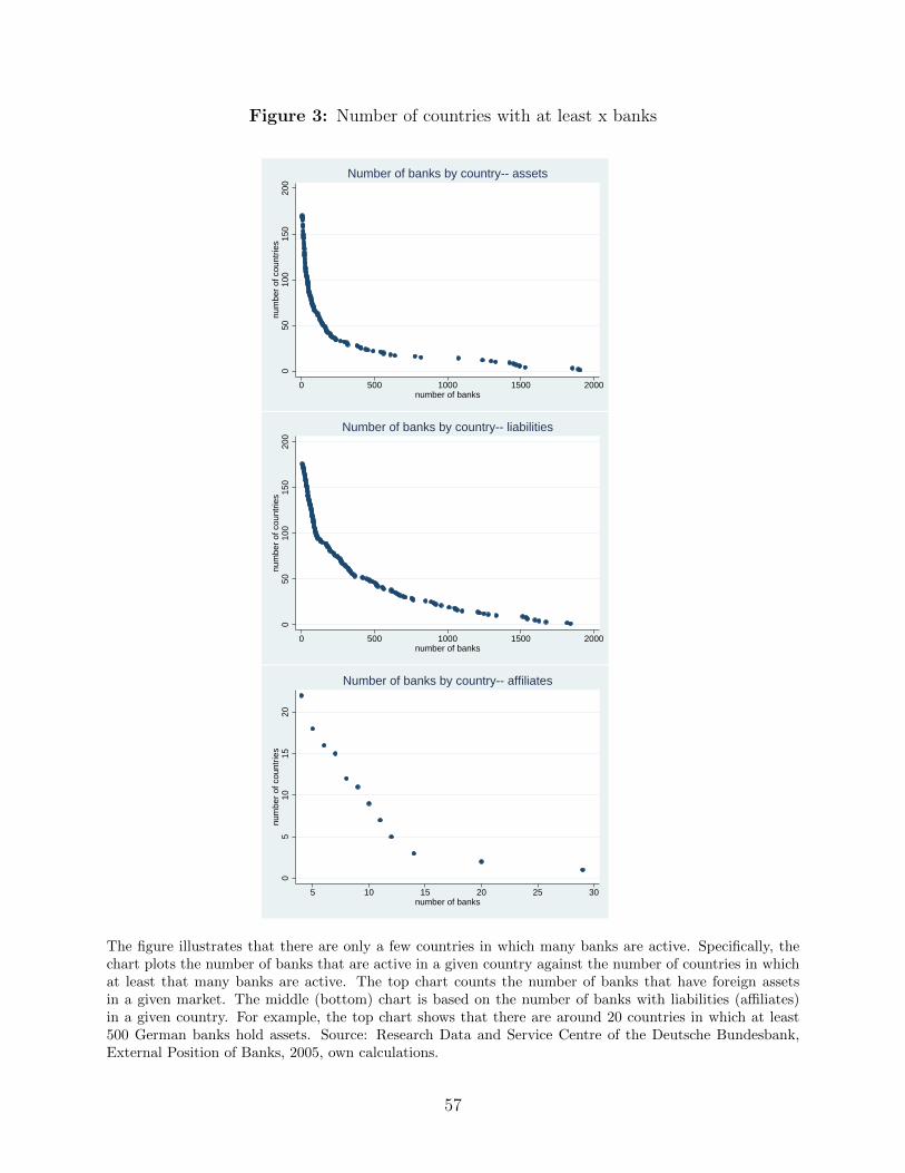
Figure 3: Number of countries with at least x banks

050

100

150

200

num

ber

of c

ount

ries

0 500 1000 1500 2000number of banks

Number of banks by country-- assets

050

100

150

200

num

ber

of c

ount

ries

0 500 1000 1500 2000number of banks

Number of banks by country-- liabilities

05

1015

20nu

mbe

r of

cou

ntrie

s

5 10 15 20 25 30number of banks

Number of banks by country-- affiliates

The figure illustrates that there are only a few countries in which many banks are active. Specifically, thechart plots the number of banks that are active in a given country against the number of countries in whichat least that many banks are active. The top chart counts the number of banks that have foreign assetsin a given market. The middle (bottom) chart is based on the number of banks with liabilities (affiliates)in a given country. For example, the top chart shows that there are around 20 countries in which at least500 German banks hold assets. Source: Research Data and Service Centre of the Deutsche Bundesbank,External Position of Banks, 2005, own calculations.

57

Figure 4: Number of banks active in at least x countries

The figure illustrates that there are only a few banks which are active in many countries. Specifically, thechart plots the number of countries that a bank is active in against the number of banks active in at leastas many countries. The top chart counts the number of countries in which a bank holds foreign assets.The middle (bottom) chart is based on the number of countries in which a bank has liabilities (affiliates).For example, the bottom chart shows that there are only 9 banks with affiliates in at least 10 countries.Source: Research Data and Service Centre of the Deutsche Bundesbank, External Position of Banks, 2005,own calculations.

58

Figure 5: Average overhead costs of German banks active abroad as a function of countrycharacteristics

The figure illustrates the strong predictive power that individual host country characteristics have for the logaverage overhead costs of German banks that operate in a given host country. Specifically, in the top chartthe average overhead costs of German banks with assets (triangle), liabilities (square) and affiliates (circle)in a country are plotted against the log GDP of the country. The middle (bottom) chart shows the sameobjects but plotted against log distance (bureaucratic quality). Source: External Position of Banks, MonthlyBalance Sheet Statistics and Income and Loss data provided by Research Data and Service Centre of theDeutsche Bundesbank, Financial Freedom Index provided by Heritage Foundation, Bureaucratic Qualityfrom Country Risk Guide provided by PRS Group, and GDP from the World Bank’s World DevelopmentIndicators, 2005, own calculations. 59