bankers without borders? implications of ring-fencing for european
TRANSCRIPT
Bankers Without Borders? Implications of Ring-Fencing for European
Cross-Border Banks
Eugenio Cerutti, Anna Ilyina, Yulia Makarova, and Christian Schmieder
WP/10/247
© 2010 International Monetary Fund WP/10/247 IMF Working Paper European Department and Monetary and Capital Markets Department
Bankers Without Borders? Implications of Ring-Fencing for European Cross-Border Banks 1
Prepared by Eugenio Cerutti, Anna Ilyina, Yulia Makarova, and Christian Schmieder
Authorized for distribution by Daniel Hardy and Inci Ötker-Robe
November 2010
Abstract
This paper presents a stylized analysis of the effects of ring-fencing (i.e., different restrictions on cross-border transfers of excess profits and/or capital between a parent bank and its subsidiaries located in different jurisdictions) on cross-border banks. Using a sample of 25 large European banking groups with subsidiaries in Central, Eastern and Southern Europe (CESE), we analyze the impact of a CESE credit shock on the capital buffers needed by the sample banking groups under different forms of ring-fencing. Our simulations show that under stricter forms of ring-fencing, sample banking groups have substantially larger needs for capital buffers at the parent and/or subsidiary level than under less strict (or in the absence of any) ring-fencing.
This Working Paper should not be reported as representing the views of the IMF. The views expressed in this Working Paper are those of the author(s) and do not necessarily represent those of the IMF or IMF policy. Working Papers describe research in progress by the author(s) and are published to elicit comments and to further debate.
JEL Classification Numbers: F34, F36, G15, G21, G28 Keywords: Cross-border banking, ring-fencing, subsidiaries, Eastern Europe Authors’ E-Mail Addresses: [email protected], [email protected], [email protected],
1 This paper benefited from comments by Bas Bakker, Jan Brockmeijer, Miroslav Kollar, Inci Otker-Robe, Daniel Hardy, Jérôme Vandenbussche, and Rachel van Elkan, as well as the participants of the MCM-EUR seminar. All errors are the authors’ own.
2
Contents Page
I. Introduction ............................................................................................................................4
II. Cross-Border Banking Groups ..............................................................................................8 A. Description of the Exercise .......................................................................................8 B. Sample Description .................................................................................................10
III. Calibration of the CESE Regional Shock ..........................................................................13 A. Country-Level Data.................................................................................................13 B. Regression Analysis ................................................................................................14 C. Calibration of NPLs and ROAs ...............................................................................15
IV. Assessing Bank Capital Needs Under Alternative Ring—Fencing Scenarios ..................17 A. Methodology ...........................................................................................................17 B. Results .....................................................................................................................20
V. Conclusions .........................................................................................................................23
References ................................................................................................................................34 Tables 1. Sample Banking Groups and Their CESE Subsidiaries ......................................................11 2. Descriptive Statistics ............................................................................................................14 3. The Dynamic Panel Regression Output for Nonperforming Loans.....................................15 4. The Dynamic Panel Regression Output for ROAs ..............................................................15 5. Country-Specific NPL Assumptions....................................................................................16 6. Country-Specific ROA Assumptions ...................................................................................17 7. Definitions of Capital Needs Under Four Ring-Fencing Scenarios .....................................19 Figures 1. A Stylized Example of a Cross-Border Banking Group—Impact of a Regional Credit Shock on Subsidiaries A, B, and C .....................................................................................9 2. A Stylized Example of a Cross-Border Banking Group—Reallocation of Funds within a Group to Cover Capital Shortfall at Subsidiary C ............................................................10 3. Total Assets of Sample CESE Subsidiaries .........................................................................12 4. Total Foreign Claims of Sample Banking Groups on the CESE Countries ........................13 5. Estimated Capital Needs Resulting From a CESE Shock— Only Indirect Exposures via Subsidiaries in the Sample .......................................................................................................21 6. Estimated Capital Needs Resulting From a CESE Shock— Indirect Exposures via Subsidiaries and Direct Cross-border Exposures ..............................................................21 7. Aggregate Capital Needs Resulting From a CESE Shock ...................................................22

3
Appendixes 1. Capital Adequacy Rates by Country and Bank Type ..........................................................24 2. Sample of LCFIs and Their Subsidiaries .............................................................................25 3. Panel Regression Analysis ...................................................................................................28 4. Interest Rates Used for Regression Analysis .......................................................................29 5. Regulatory Minimum Capital Requirements by Country ....................................................30 6. Loss Given Default Ratios in the CESE countries...............................................................31 7. Using BIS Data to Capture Remaining LCFIs’ Exposure to CESE ....................................32 8. Analysts’ Estimates of Losses and Capital Needs ...............................................................33 Appendix Tables A1.1 Average CARs of Foreign Sample Subsidiaries vs. the Country-Level Average CARs ...............................................................................................................24 A2.1. Sample Description ........................................................................................................25 A3.1 Panel Regression Analysis (Dependent Variable: NPLs) ...............................................28 A4.1 Overview on Data Sources for Short-Term Interest Rates .............................................29 A5.1. Regulatory Minimum Capital Requirements in the CESE Countries ............................30 A6.1. Loss Given Default Ratios by Country ..........................................................................31 A8.1. Private Analysts’ Estimates of Losses and Capital Needs of Western ..........................33
4
I. INTRODUCTION
The concept of centralized capital and liquidity management by internationally active banks was challenged by the recent crisis, sparking a debate about the desirable organizational and regulatory arrangements for cross-border banking groups. This paper focuses on the costs for these banking groups that are associated with different restrictions on intra-group cross-border transfers imposed by the host/home country regulators (henceforth referred to as “ring-fencing”). More specifically, it provides a stylized analysis of how much additional capital might be needed if the banking groups are restricted, to different degrees, in their ability to re-allocate funds across jurisdictions following a credit shock affecting their lending activities in a given region. The paper does not estimate the group level potential recapitalization needs under an extreme scenario (which is typically done in a stress test), but rather considers the implications of adverse economic conditions for cross-border banking groups under different forms of ring-fencing. The analysis is based on bank-level data for European banking groups and their subsidiaries in Central, Eastern, and Southern Europe (CESE).2 At present, a number of European countries have legal restrictions on intra-group cross-border asset transfers. These limits are aimed at preventing undue influence by a foreign parent on its subsidiaries (e.g., in the form of disproportionate transfers of assets that could potentially trigger solvency or liquidity problems), or aimed at protecting the interests of minority shareholders and creditors of subsidiaries (European Commission, 2010). In order to ring-fence the subsidiary from the rest of the group, the host country can target the subsidiary’s ability to transfer funds abroad directly or indirectly, through measures affecting the entire domestic banking system (e.g., stopping the distribution of dividends by all banks during a crisis).3 During 2008–09, many subsidiaries of European banking groups had to rely on their foreign parents for capital and liquidity support. There is some evidence that, ex ante, the CESE subsidiaries had expected that they could rely on parent banks in case of need (e.g., the average capitalization levels of the foreign-owned subsidiaries in most CESE countries were 1 to 2 percentage points lower than the banking system averages at the outset of the crisis (Appendix 1)). Ex post, these expectations were validated by the assistance provided by
2 The interbank linkages in this region and their role in transmitting or mitigating shocks have been recently analyzed in Arvai, Driessen, and Otker-Robe (2009); Hermann and Mihaljek (2010); and Maechler and Ong (2009), but the analysis relied mainly on the country-level (not bank-level) data on cross-border bank exposures. 3 The current initiatives at the EU level aim to achieve the dual objective of (i) preventing the risk of insolvency that could potentially be generated by a disproportionate transfer of assets for the credit institution making the transfer; and (ii) lifting restrictions on transfers of assets if such transfers can potentially limit the extent of a crisis (European Commission, 2010).
5
parent banks.4 Yet, in order to maintain financial and economic stability, the regulators in many host countries tightened restrictions on intra-group cross-border transfers, limiting the ability of cross-border banking groups to re-allocate funds from subsidiaries with excess capital (liquidity) to those that were in need of capital (liquidity).5 There are arguments both for and against ring-fencing. The arguments in favor of centralized cross-border bank structures and against ring-fencing rely on efficiency and financial stability considerations (e.g., benefits of diversification across country-specific shocks). From a cross-border bank’s perspective, the ability to freely re-allocate funds across its affiliates is essential for achieving the most efficient outcome—a point emphasized in the recent report prepared by the Institute of International Finance (IIF, 2010). Centralized cross-border bank structures may yield benefits for the host country economies as well. De Haas and van Lelyveld (2010), for example, show that the ability of international banks to attract liquidity and raise capital allows them to operate an internal capital market, which provides their subsidiaries with better access to capital and liquidity than what they would have been able to achieve on a stand-alone basis, and hence may help to reduce the pressure to scale back lending during economic downturns. For both home and host authorities, the absence of ring fencing facilitates diversification and can thus make the group as a whole more stable, for example, against shocks in the home country. However, there are also arguments in favor of ring-fencing. For a host country regulator, the decision to impose ring-fencing would typically be driven by macro-financial stability considerations, such as the need to protect the domestic banking system from negative spillovers from the rest of the group, or more generally, to increase reserves for the whole domestic banking system during a crisis when the magnitude of the impending output collapse and bank losses are uncertain. The possibility of contagion from a parent bank to subsidiaries in the European context was recently analyzed by Popov and Udell (2010), who showed that the contraction of banks’ balance sheets caused by losses and/or a deterioration
4 See, for example, the recent “Statement at the end of the European Bank Coordination Initiative’s Second Full Forum Meeting,” Press Release No. 10/106, March 22, 2010. In the context of this initiative, the large bank groups with systemic presence in several CESE countries have committed to maintain their exposure and keep their subsidiaries well capitalized (http://www.imf.org/external/np/sec/pr/2010/pr10106.htm). 5 To name a few examples, bank regulators in Croatia, Poland, and Turkey recommended the non-distribution of profits by the subsidiaries of foreign banks despite relatively strong bank fundamentals. In the case of Croatia, the CNB Governor, Dr. Željko Rohatinski, at a press conference held on February 18, 2009 said that “the CNB would not look favorably upon attempts to withdraw capital, deposits, or pay out total accumulated profits, because that would destabilize the domestic banking system. In such a case, the CNB would be forced to undertake protective measures, regardless of thus connected risks.” In the case of Turkey, the head of the banking regulation agency stated in December 2009 that “it is our natural right to expect those profits generated in this country to be invested and used in credit extension again in this country.” Banks in Turkey were expected to consult the regulator before distributing any dividends during the last two years. The IMF Article IV report on Poland (2010) classified the regulator’s recommendation for subsidiaries of foreign banks to refrain from paying out dividends, despite robust capital buffers, as a form of capital control.

6
in bank solvency was transmitted across borders to Eastern Europe by Western European banking groups in the early stages of the 2007–08 crisis. Moreover, the difficulties in resolving cross-border banking groups and the absence of agreements on burden-sharing mechanisms during the crisis triggered a discussion about the desirability of promoting greater self-sufficiency of banking groups’ affiliates in normal and in crisis times. Hoelscher, Hsu, Otker-Robe, and Santos (2010) considers the pros and cons of the so-called stand-alone subsidiarization (SAS) approach, according to which a cross-border banking group should be set up as a network of fully self-sufficient national subsidiaries. The authors note that from a banking group’s perspective, the SAS approach may be beneficial if it can provide additional incentives for subsidiaries to better manage liquidity and credit risk. From the host/home country perspective, the key benefits of SAS include limiting intra-group contagion and allowing selective resolution of problem parts of the group with minimal disruption for the rest of the group. Leaving aside the question of the potential benefits of imposing greater autonomy on the banking group’s affiliates operating in different jurisdictions, this paper focuses on the costs of ring-fencing for cross-border banking groups under different forms of ring-fencing. The cost is measured in terms of the amount of external capital that is required to cover capital shortfalls faced by the affiliates of these groups as a result of a credit shock. More specifically, this paper estimates the amount of additional capital that might be needed if the sample banking groups are restricted in their ability to re-allocate excess profits and/or capital across jurisdictions following a credit shock that affects some of the affiliates within these groups.6 It should be noted that the transfers of excess profits/capital are not the only mechanisms through which banking groups could manage the level of capitalization of their affiliates. For example, the latter could also be achieved through capital injections via subordinated debt or by “shifting” assets (instead of capital) between different parts of the group.7 However, the empirical analysis of these alternative mechanisms is constrained by the lack of publicly available bank-level data on intra-group lending and asset transfers. That said, the conclusions that such exercises might yield are likely to be quite similar to the results regarding the transfers of excess capital/profit presented here. Three different types of ring-fencing are considered in this paper, ranging from partial ring-fencing to full ring-fencing. Partial ring-fencing assumes that only excess profits of
6 The issue of intra-group liquidity transfers is not considered in this paper. It is left for future research. 7 At the onset of the crisis, many European parent banks had direct cross-border loans on their books, which sometimes had been purchased from the subsidiaries in the boom years. There is anecdotal evidence that suggests that the reverse happened during the crisis; that is, in some cases, subsidiaries with large capital buffers bought back loans from the parent banks, thereby, reducing their capital adequacy ratios (CARs).

7
subsidiaries, but not their excess capital buffers, can be re-allocated within a group. Near-complete ring-fencing assumes that only transfers from the parent to a subsidiary are allowed. Full ring-fencing corresponds to the strict standalone subsidiarization (SAS) model, where no intra-group transfers are allowed. The analysis presented below takes into account the parent banks’ ownership stakes in their subsidiaries. The sample of banks included in the analysis consists of 25 European banking groups and their 113 subsidiaries located in 18 countries in CESE. There are several reasons for using this sample: (i) most of these banks have a large network of subsidiaries operating in several countries in CESE region; and (ii) the fact that many countries in the region were severely hit by the crisis allows us to illustrate a range of outcomes under different ring-fencing assumptions, given a severe, but realistic credit shock affecting parts of these banking groups. The individual bank-level data on branches are not used in the estimation because branches are not stand-alone entities, which makes it difficult for the host country authorities to ring fence them. The CESE exposures via branches are analyzed as part of the total direct cross-border exposures of parent banks.8 Qualitatively, the results of the analysis are fairly intuitive: any type of restrictions on intra-group transfers would entail the need for additional, and possibly significant, capital buffers at the subsidiary and/or the parent bank level of cross-border banking groups. Quantitatively, the sample banks’ capital needs resulting from a simulated credit shock affecting their CESE subsidiaries over the 2009–2010 period are 1.5–3 times higher in the ring-fencing/SAS scenarios than those under no ring-fencing. These results are robust to variations in the methodology for computing capital needs, including the post-shock adjustment in risk-weighted assets (standardized versus the Basel II Internal Ratings Based (IRB) approach). What are the policy implications of this analysis? First, the establishment of a credible framework for the resolution of cross-border banking groups would help to avoid unilateral and likely more costly solutions (in terms of capital requirements). This is because the existence of such a framework could reduce the incentives for and the incidence of ring-fencing by the home/host country authorities. Second, in the absence of such resolution and burden-sharing mechanisms, setting the minimum capital requirements for cross-border banking groups would have to take into account the potential presence of ring-fencing,
8 The choice between branches and subsidiaries has been analyzed in the literature. Cerutti, Dell’Ariccia, and Martinez-Peria (2007), for example, found that cross-border banking groups are more likely to set up a branch than a subsidiary in host countries with relatively higher corporate taxes, since this makes it easier to transfer profits across borders. Other considerations in the choice between branches and subsidiaries were (i) branches are more common when foreign operations are smaller in size and do not have a retail orientation; (ii) branches are less common in countries with highly risky macroeconomic environments, where parent banks seem to prefer the ‘‘hard’’ shield of limited liability provided by subsidiaries; (iii) foreign banks tend to specialize in one organizational form or the other, beyond what is explained by their home-country regulation; and (iv) foreign banks are less likely to operate as branches in countries that limit their activities and where regulation makes it difficult to establish new banks.
8
especially in crisis times. Such a possibility may force cross-border banks to gravitate towards organizational structures that are more immune to ring-fencing (either SAS-type structures or branch structures). Third, should regulators decide to promote a SAS-like approach, its potential benefits would have to be carefully weighed against its potential costs. The rest of the paper is organized as follows. Section II provides a description of the exercise and the data. Section III explains the calibration of the credit shock affecting CESE subsidiaries. Section IV presents the methodology for calculating capital needs, as well as the main results under different ring-fencing scenarios. Section V draws conclusions and discusses policy implications.
II. CROSS-BORDER BANKING GROUPS
A. Description of the Exercise Consider a stylized cross-border banking group that has subsidiaries operating in countries A, B, and C (Figure 1). Suppose that countries A, B, and C are affected by a regional shock that leads to a significant deterioration in the credit quality of the loan books of subsidiaries operating in these countries. Suppose that losses resulting from this shock are offset by profits and capital buffers held by each of these subsidiaries (as a first line of defense) and by funds transferred from the rest of the group (as a second line of defense). The capital needs resulting from the CESE credit shock are estimated in two steps: (i) For each subsidiary, the capital need is defined as the amount of capital required to
bring its post-shock CAR back to either the country-specific (Basel II) regulatory minimum or to the subsidiary-specific pre-shock level.9 The latter is conservative in that it requires subsidiaries not to run down pre-shock buffers.
(ii) At the group level, total capital needs are computed by adding up all the capital needs of individual subsidiaries (and also losses on direct cross-border exposures of parent banks, in some simulations) and offsetting them against any other funds (i.e., excess profits and/or capital) that can be re-allocated from other parts of the banking group.
Hence, the resulting total capital needs at the group level depend on the availability of excess profits and/or capital in the subsidiaries and parent bank, as well as on the degree to which these funds (excess profits and/or capital) can be re-allocated within a group.
9 The post shock CAR is estimated by taking into account actual or projected losses, provisions, capital buffers, and possible increases in risk-weighted assets.

9
Figure 1. A Stylized Example of a Cross-Border Banking Group—Impact of a Regional Credit Shock on Subsidiaries A, B, and C
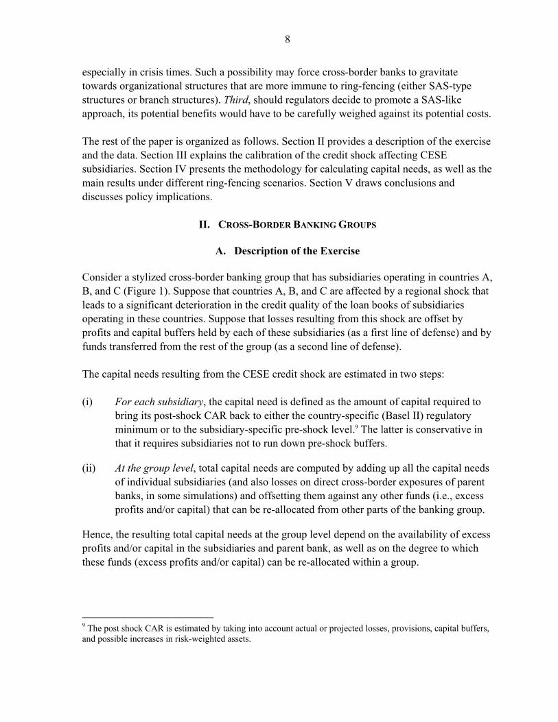
Suppose that as a result of the shock, one of the three subsidiaries (Sub C in Figure 2) experiences a capital shortfall (i.e., its regulatory capital falls below the national minimum capital requirement). Then, the extent to which this subsidiary can be recapitalized using the funds transferred from other parts of the group (i.e., without having to raise fresh capital) would depend on the existence of restrictions on such transfers (i.e., on the degree of ring-fencing). Four ring-fencing scenarios are analyzed in this paper and illustrated in Figure 2: 1) The no ring-fencing scenario assumes that parent bank’s profits, as well as
subsidiaries’ excess profits and excess capital buffers can be used to cover capital shortfall in any of the subsidiaries.
2) The partial ring-fencing scenario assumes that parent bank’s profits and only subsidiaries’ excess profits, but not excess capital, can be re-allocated within a group.
3) The near-complete ring-fencing scenario assumes that only transfers from the parent to any of the subsidiaries are allowed.
4) The full ring fencing, i.e., stand-alone subsidiarization SAS, assumes that no transfers between any of the group’s affiliates (including from the parent bank to subsidiaries) can take place.
Parent Bank Sub A Sub B Sub C
Losses (net of provisions) at each of the subs
Sub A Sub B Sub C
Regional shock
BuffersProfits and Capital at each of the subs
Sub A Sub B Sub COutcome
Recap needs (if any) at each of the subs
Sub A Sub B Sub C
10
Figure 2. A Stylized Example of a Cross-Border Banking Group—Reallocation of Funds within a Group to Cover Capital Shortfall at Subsidiary C
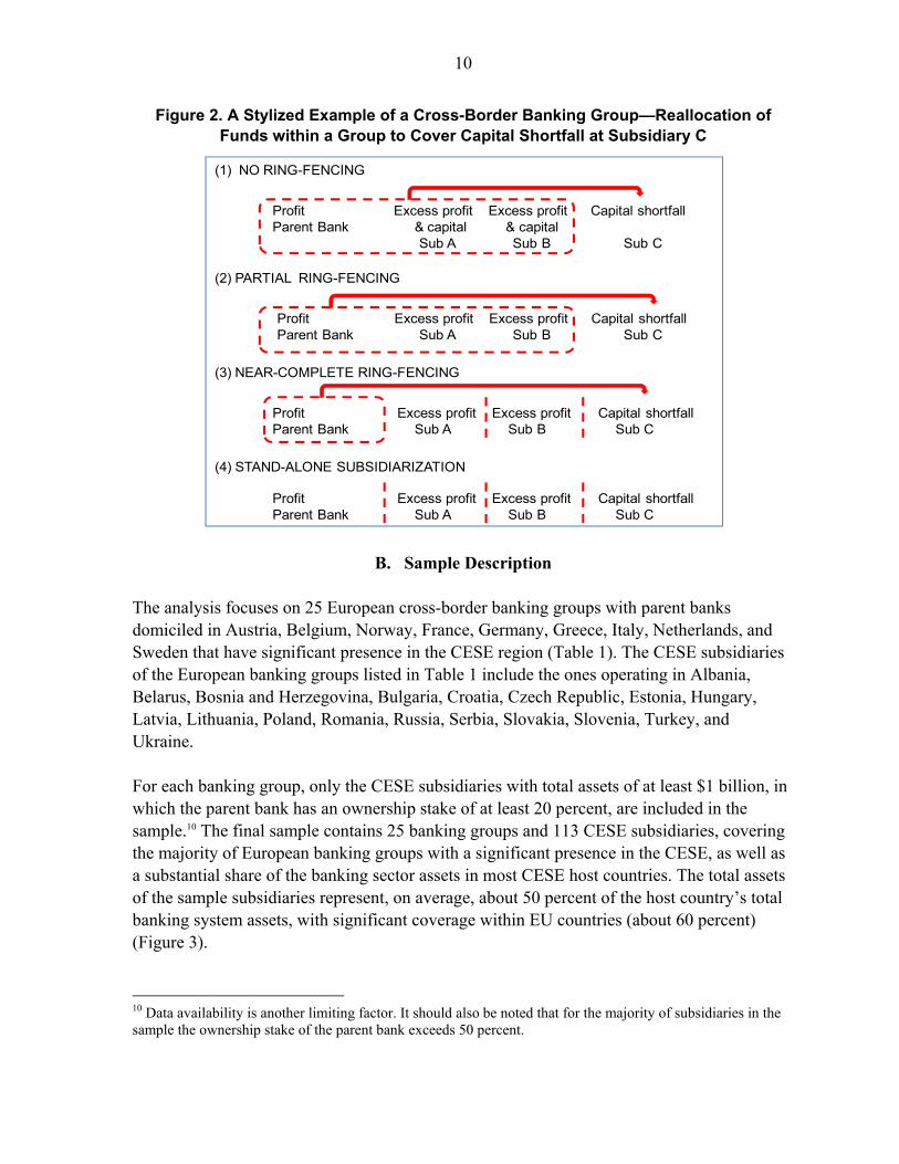
B. Sample Description The analysis focuses on 25 European cross-border banking groups with parent banks domiciled in Austria, Belgium, Norway, France, Germany, Greece, Italy, Netherlands, and Sweden that have significant presence in the CESE region (Table 1). The CESE subsidiaries of the European banking groups listed in Table 1 include the ones operating in Albania, Belarus, Bosnia and Herzegovina, Bulgaria, Croatia, Czech Republic, Estonia, Hungary, Latvia, Lithuania, Poland, Romania, Russia, Serbia, Slovakia, Slovenia, Turkey, and Ukraine. For each banking group, only the CESE subsidiaries with total assets of at least $1 billion, in which the parent bank has an ownership stake of at least 20 percent, are included in the sample.10 The final sample contains 25 banking groups and 113 CESE subsidiaries, covering the majority of European banking groups with a significant presence in the CESE, as well as a substantial share of the banking sector assets in most CESE host countries. The total assets of the sample subsidiaries represent, on average, about 50 percent of the host country’s total banking system assets, with significant coverage within EU countries (about 60 percent) (Figure 3).
10 Data availability is another limiting factor. It should also be noted that for the majority of subsidiaries in the sample the ownership stake of the parent bank exceeds 50 percent.
Profit Excess profit Excess profit Capital shortfallParent Bank & capital & capital
Sub A Sub B Sub C
(1) NO RING-FENCING
(2) PARTIAL RING-FENCING
Profit Excess profit Excess profit Capital shortfallParent Bank Sub A Sub B Sub C
(3) NEAR-COMPLETE RING-FENCING
Profit Excess profit Excess profit Capital shortfallParent Bank Sub A Sub B Sub C
Profit Excess profit Excess profit Capital shortfallParent Bank Sub A Sub B Sub C
(4) STAND-ALONE SUBSIDIARIZATION

11
Table 1. Sample Banking Groups and Their CESE Subsidiaries (A circle may indicate the presence of more than one subsidiary) 11
Sources: Bankscope and Bank reports. Notes: 1/ Subsidiary of Unicredit and 2/ Subsidiary of BayernLB.
11 See Appendix 2 for a detailed description of the sample.
Parent Bank Parent bank's home country S
lov
enia
Cze
ch
Re
p.
Slo
vak
ia
Po
lan
d
Tu
rke
y
Bu
lga
ria
Ro
ma
nia
Hu
ng
ary
Alb
an
ia
Bo
sn
ia
Cro
ati
a
Ser
bia
Es
ton
ia
La
tvia
Lit
hu
an
ia
Ru
ss
ia
Uk
rain
e
Be
laru
s
Erste Group Bank Austria
RZB Austria
Volksbank Austria
Bank Austria 1/ Austria
Hypo Alpe Adria Group 2/ Austria
Dexia Belgium
KBC Bank Belgium
DNB NOR Norway
BNP Paribas France
Société Générale France
Crédit Agricole France
Bayern LB Germany
Commerzbank Germany
Deutsche Bank Germany
Alpha Bank Greece
EFG Eurobank Greece
NBG Greece
Piraeus Bank Greece
Allied Irish Banks Ireland
Intesa Sanpaolo Italy
UniCredit SpA Italy
ING Bank Netherlands
Nordea Bank Sweden
SEB Sweden
Swedbank Sweden
Subsidiaries
Central Europe
Southern and South-Eastern
Europe Baltic
Countries CISSouthern Europe
(Balkans)
12
Figure 3. Total Assets of Sample CESE Subsidiaries (in percent of total banking assets of the host country, December 2008)
Source: Bankscope, national authorities, and staff estimates.
That said, the total assets of subsidiaries included in the sample do not necessarily capture the full CESE exposures of these banking groups. This is because the latter could also include the parent banks’ direct cross-border lending to CESE countries, as well as lending by the branches operating in the host countries alongside the subsidiaries.12 In order to capture these exposures, the aggregate BIS data on foreign claims by reporting banks on the CESE countries are used to impute the residual exposures of the banking groups to the CESE countries, including both direct cross-border exposures and exposures through branches (Figure 4). The data used for this purpose comes from the BIS consolidated international banking statistics (see Appendix 7 for details). For each banking group, end-2008 data on total assets, total customer loans, profits, nonperforming loans (NPLs), loan loss provisions, regulatory capital, Tier 1 capital and risk-weighted assets were collected at the group level, at the parent bank level and at the level of individual CESE subsidiaries (when available). The main data sources include Bankscope, Bloomberg, as well as individual bank reports.
12 There are some cross-border banking groups that conduct mainly direct cross-border lending instead of lending through subsidiaries/branches (see McCauley, McGuire, and von Peter, 2010).
0
10
20
30
40
50
60
70
80
90
100
Slo
ven
ia
Cze
ch R
ep
Slo
vaki
a
Po
lan
d
Turk
ey
Bu
lgar
ia
Ro
man
ia
Hu
nga
ry
Alb
ania
Bo
snia
Cro
atia
Serb
ia
Esto
nia
Latv
ia
Lith
uan
ia
Ru
ssia
Ukr
ain
e
Be
laru
s

13
Figure 4. Total Foreign Claims of Sample Banking Groups on the CESE Countries (in percent of host country GDP, December 2008)
Sources: Bankscope, national authorities, BIS and staff estimates. 1/ Calculated as a residual from total foreign claims (see Appendix 7).
III. CALIBRATION OF THE CESE REGIONAL SHOCK
A. Country-Level Data
The CESE credit shock is modeled as deterioration in macroeconomic conditions during 2009–10 leading to an increase in NPLs and a decrease in the return on assets (ROAs) of the CESE subsidiaries. The simulation of the shock relies largely on the actual data for 2009 and on projections for the CESE country-level NPLs and ROAs for 2010, which assume a slower economic recovery than the one envisaged in the April 2010 IMF’s World Economic Outlook (WEO) forecasts. Changes in NPLs and ROAs are linked to the changes in macroeconomic conditions via panel regression models. The rationale behind this approach is to use consistent data across countries to come up with a specification that captures historical NPL and ROA patterns in the CESE region rather than fitting country-specific dynamics separately or extrapolating from past crises that occurred in other regions. The panel regression analysis uses annual data for all CESE countries for the period of 1999–2009. The data for the dependent variable, aggregate NPLs at the country level, comes from the IMF’s Global Financial Stability Reports (IMF, 2009, Table 24). The data are examined for possible structural breaks and inconsistencies in the NPL definitions across countries.13
13 See Appendix 3 for details.
0
20
40
60
80
100
120
140
Slo
ven
ia
Cze
ch R
ep
Slo
vaki
a
Po
lan
d
Turk
ey
Bu
lgar
ia
Ro
man
ia
Hu
nga
ry
Alb
ania
Bo
snia
Cro
atia
Serb
ia
Esto
nia
Latv
ia
Lith
uan
ia
Ru
ssia
Ukr
ain
e
Be
laru
s
Direct cross-border and branches claims 1/
Total customer loans of sample subsidiaries
14
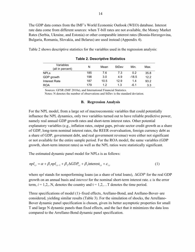
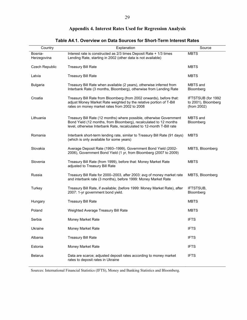
The GDP data comes from the IMF’s World Economic Outlook (WEO) database. Interest rate data come from different sources: when T-bill rates are not available, the Money Market Rates (Serbia, Ukraine, and Estonia) or other comparable interest rates (Bosnia-Herzegovina, Bulgaria, Romania, Slovakia, and Belarus) are used instead (Appendix 4). Table 2 shows descriptive statistics for the variables used in the regression analysis:
Table 2. Descriptive Statistics
Variables (all in percent)
N Mean StDev Min. Max.
NPLs 185 7.6 7.3 0.2 35.8 GDP growth 198 3.0 4.9 -18.5 12.2 Interest Rate 187 10.5 12.9 1.4 93.2 ROA 179 1.2 1.3 -6.1 3.3
Sources: GFSR (IMF 2010a), and International Financial Statistics. Notes: N denotes the number of observations and StDev is the standard deviation.
B. Regression Analysis
For the NPL model, from a large set of macroeconomic variables that could potentially influence the NPL dynamics, only two variables turned out to have reliable predictive power, namely real annual GDP growth rates and short-term interest rates. Other potential explanatory variables (e.g., inflation rates, output gaps, private sector credit growth as a share of GDP, long-term nominal interest rates, the REER overvaluation, foreign currency debt as a share of GDP, government debt, and real government revenue) were either not significant or not available for the entire sample period. For the ROA model, the same variables (GDP growth, short-term interest rates) as well as the NPL ratios were statistically significant.
The estimated dynamic panel model for NPLs is as follows:
titititi GDPnplnpl ,ti,3,21,1, interest (1)
where npl stands for nonperforming loans (as a share of total loans), GDP for the real GDP growth on an annual basis and interest for the nominal short-term interest rate. is the error term, i = 1,2,..N, denotes the country and t = 1,2,…T denotes the time period.
Three specifications of model (1)–fixed effects, Arellano-Bond, and Arellano-Bover–are considered, yielding similar results (Table 3). For the simulation of shocks, the Arrellano-Bover dynamic panel specification is chosen, given its better asymptotic properties for small T and large N dynamic panels than fixed effects, and the fact that it minimizes the data loss compared to the Arrellano-Bond dynamic panel specification.
15
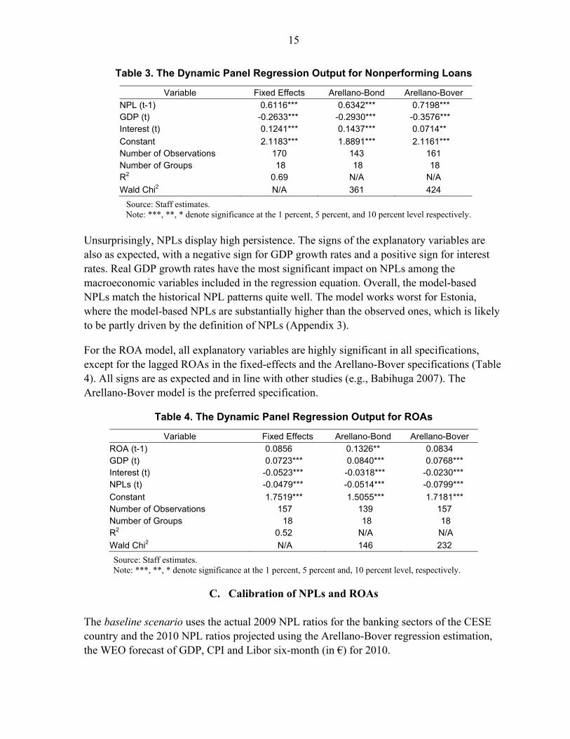
Table 3. The Dynamic Panel Regression Output for Nonperforming Loans
Variable Fixed Effects Arellano-Bond Arellano-Bover
NPL (t-1) 0.6116*** 0.6342*** 0.7198*** GDP (t) -0.2633*** -0.2930*** -0.3576*** Interest (t) 0.1241*** 0.1437*** 0.0714**
Constant 2.1183*** 1.8891*** 2.1161*** Number of Observations 170 143 161 Number of Groups 18 18 18 R2 0.69 N/A N/A
Wald Chi2 N/A 361 424
Source: Staff estimates. Note: ***, **, * denote significance at the 1 percent, 5 percent, and 10 percent level respectively.
Unsurprisingly, NPLs display high persistence. The signs of the explanatory variables are also as expected, with a negative sign for GDP growth rates and a positive sign for interest rates. Real GDP growth rates have the most significant impact on NPLs among the macroeconomic variables included in the regression equation. Overall, the model-based NPLs match the historical NPL patterns quite well. The model works worst for Estonia, where the model-based NPLs are substantially higher than the observed ones, which is likely to be partly driven by the definition of NPLs (Appendix 3).
For the ROA model, all explanatory variables are highly significant in all specifications, except for the lagged ROAs in the fixed-effects and the Arellano-Bover specifications (Table 4). All signs are as expected and in line with other studies (e.g., Babihuga 2007). The Arellano-Bover model is the preferred specification.
Table 4. The Dynamic Panel Regression Output for ROAs
Variable Fixed Effects Arellano-Bond Arellano-Bover
ROA (t-1) 0.0856 0.1326** 0.0834 GDP (t) 0.0723*** 0.0840*** 0.0768*** Interest (t) -0.0523*** -0.0318*** -0.0230*** NPLs (t) -0.0479*** -0.0514*** -0.0799***
Constant 1.7519*** 1.5055*** 1.7181*** Number of Observations 157 139 157 Number of Groups 18 18 18 R2 0.52 N/A N/A
Wald Chi2 N/A 146 232
Source: Staff estimates. Note: ***, **, * denote significance at the 1 percent, 5 percent and, 10 percent level, respectively.
C. Calibration of NPLs and ROAs The baseline scenario uses the actual 2009 NPL ratios for the banking sectors of the CESE country and the 2010 NPL ratios projected using the Arellano-Bover regression estimation, the WEO forecast of GDP, CPI and Libor six-month (in €) for 2010.

16
The adverse scenario uses the actual NPL data for 2009 (as in the baseline) and the 2010 NPL projections based on the assumption that for each of the CESE countries, the 2010 GDP growth rate is 2 percentage points lower than the 2010 April WEO GDP growth rate forecasts and the 2010 interest rate is 200 basis points higher than in 2009. Given the dominant role of GDP in the regression specification that is used to calibrate the shock, the adverse scenario features a slow recovery and high NPLs in both years, with most of the NPL increase taking place in 2009. The NPLs estimated under the 2010 baseline scenario are broadly in line with the estimates in the GFSR (April 2010, IMF 2010a).14 Overall, the adverse scenario can be characterized as relatively “mild” among the plausible adverse scenarios, not necessarily too far away from the baseline (Table 5).
Table 5. Country-Specific NPL Assumptions
2008 Median
2009 Median 1/
2010 Baseline Median 2/
2010 Adverse Median 3/
Baltic countries 3.6 16.4 15.9 16.8 CEE-3 3.3 5.6 5.9 7.0 CIS 3.8 9.6 8.1 9.1 SEE 4.3 6.4 7.4 8.3
Source: Staff estimates.
1/ The 2009 provisional data come from IMF, 2010, Table 24; 2/ Baseline scenario uses NPLs estimated via dynamic panel regression using CESE 1999–2008 data. WEO assumptions are used for out-of-sample forecasts; 3/ Adverse scenario assumes a slow recovery, i.e., 2010 GDP growth is 2 percentage points below the 2010 WEO GDP growth forecasts, and interest rates are 200 bps higher than in 2009.
For subsidiaries, 2009–10 profits are calculated by taking the actual 2008 pre-provision profits of individual subsidiaries as a base and applying the same rate of change as that of the country level ROAs calculated based on the regression model (Table 6). The regression based estimates of ROAs are adjusted downward for Slovenia, Slovakia, Belarus and Bosnia-Herzegovina and upward for Romania and Bulgaria.15
14 The averse scenario used in this paper is somewhat less severe than the adverse growth scenario in the GFSR (April 2010, IMF 2010a), with NPLs that are 3–5 percentage points lower for the CEEs, SEEs and the Baltic states. For the CIS, the figures are comparable, as the figures in this paper include Belarus (with low NPLs), whereas the GFSR did not. 15 The adjustment accounts for the fact that the returns have been lower (first group of countries) or higher (Romania and Bulgaria) than on average in the sample in the past, which could be triggered by the level of competition, for example. The adjustment was 0.4 (Bulgaria) and 0.7 (Romania) in positive terms as well as 0.5 (Belarus and Slovakia) and 0.7 (Bosnia-Herzegovina and Slovenia) in negative terms.

17
Table 6. Country-Specific ROA Assumptions
2008 Median
2009 Median /1
2010 Baseline Median 2/
2010 Adverse Median 3/
Baltic countries 1.2 -0.1 0.0 -0.2 CEE-3 1.2 1.1 1.2 1.0 CIS 1.4 0.5 1.0 0.8 SEE 1.7 0.9 1.0 0.8
Source: Staff estimates. 1/ The 2009 provisional data come from IMF, 2010, Table 24; 2/ Baseline scenario uses ROAs estimated via dynamic panel regression using CESE 1999–2008 data; 3/ Adverse scenario assumes a slow recovery, i.e., 2010 GDP growth is 2 percentage points below the 2010 WEO GDP growth forecasts, and interest rates are 200 bps higher than in 2009.
For parent banks, the 2009 net profits are either the actual numbers or estimates based on market consensus forecasts.16 The 2010 profits are assumed to be equal to the 2009 profits, provided that the latter were positive, and zero otherwise. While this assumption is ad hoc, it is fairly neutral and is unlikely to introduce an upward bias in the estimates of capital needs.
IV. ASSESSING BANK CAPITAL NEEDS UNDER ALTERNATIVE RING—FENCING
SCENARIOS
A. Methodology
This section presents the method applied to calculate capital adequacy under stress, and capital requirements, respectively. The loan loss reserve (LLR) for subsidiary k located in a CESE country i following a credit shock is as follows:
, , ,Post-shock LLR NPL *E *LGDk i k i k i i
(2)
where ,NPLk i is the post-shock NPL ratio17 (nonperforming loans in percent of total
exposure), ,E k i is the total exposure (customer loans), and LGDi is the loss given default
(assumed to be the same for all subsidiaries operating in country i). Because bank-level end-2008 NPL data are not available for the majority of subsidiaries in the sample, the country-level end-2008 NPL ratios are used to proxy for the pre-shock bank-level NPL ratios. Country-specific LGDs come from the World Bank’s Doing Business webpage. In order to
16 Parent banks’ net profits are used because parent bank’ non-CESE-related losses are not explicitly included in the simulations. As explained at the end of the next section, some adjustments are needed to parent banks’ net profits when including parent banks’ direct cross-border CESE losses to avoid double counting. 17 The stock (rather than the flow) of NPLs is considered in order to account for both possible under-provisioning as well as provisions on additional NPLs.
18
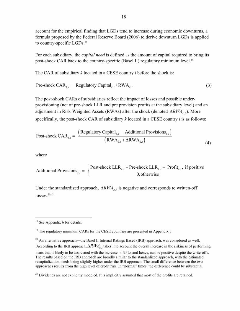
account for the empirical finding that LGDs tend to increase during economic downturns, a formula proposed by the Federal Reserve Board (2006) to derive downturn LGDs is applied to country-specific LGDs.18 For each subsidiary, the capital need is defined as the amount of capital required to bring its post-shock CAR back to the country-specific (Basel II) regulatory minimum level.19 The CAR of subsidiary k located in a CESE country i before the shock is:
, , ,Pre-shock CAR Regulatory Capital / RWAk i k i k i
(3)
The post-shock CARs of subsidiaries reflect the impact of losses and possible under-provisioning (net of pre-shock LLR and pre provision profits at the subsidiary level) and an
adjustment in Risk-Weighted Assets (RWAs) after the shock (denoted ikRWA , ). More
specifically, the post-shock CAR of subsidiary k located in a CESE country i is as follows:
, ,
,
, ,
Regulatory Capital Additional ProvisionsPost-shock CAR
RWA RWAk i k i
k i
k i k i
(4)
where
, , ,,
Post-shock LLR Pre-shock LLR Profit , if positive Additional Provisions
0,otherwisek i k i k i
k i
Under the standardized approach, ikRWA , is negative and corresponds to written-off
losses.20, 21
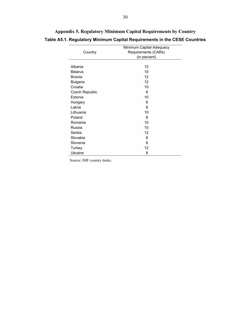
18 See Appendix 6 for details. 19 The regulatory minimum CARs for the CESE countries are presented in Appendix 5. 20 An alternative approach—the Basel II Internal Ratings Based (IRB) approach, was considered as well.
According to the IRB approach, ,k iRWA takes into account the overall increase in the riskiness of performing
loans that is likely to be associated with the increase in NPLs and hence, can be positive despite the write-offs. The results based on the IRB approach are broadly similar to the standardized approach, with the estimated recapitalization needs being slightly higher under the IRB approach. The small difference between the two approaches results from the high level of credit risk. In “normal” times, the difference could be substantial. 21 Dividends are not explicitly modeled. It is implicitly assumed that most of the profits are retained.
19
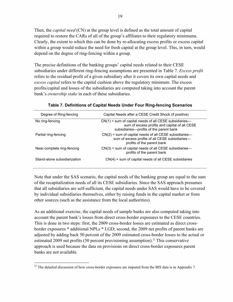
Then, the capital need (CN) at the group level is defined as the total amount of capital required to restore the CARs of all of the group’s affiliates to their regulatory minimums. Clearly, the extent to which this can be done by re-allocating excess profits or excess capital within a group would reduce the need for fresh capital at the group level. This, in turn, would depend on the degree of ring-fencing within a group. The precise definitions of the banking groups’ capital needs related to their CESE subsidiaries under different ring-fencing assumptions are presented in Table 7. Excess profit refers to the residual profit of a given subsidiary after it covers its own capital needs and excess capital refers to the capital cushion above the regulatory minimum. The excess profits/capital and losses of the subsidiaries are computed taking into account the parent bank’s ownership stake in each of these subsidiaries.
Table 7. Definitions of Capital Needs Under Four Ring-fencing Scenarios
Degree of Ring-fencing Capital Needs after a CESE Credit Shock (if positive)
No ring-fencing
CN(1) = sum of capital needs of all CESE subsidiaries— sum of excess profits and capital of all CESE
subsidiaries—profits of the parent bank
Partial ring-fencing
CN(2) = sum of capital needs of all CESE subsidiaries— sum of excess profits of all CESE subsidiaries—
profits of the parent bank
Near-complete ring-fencing
CN(3) = sum of capital needs of all CESE subsidiaries— profits of the parent bank
Stand-alone subsidiarization CN(4) = sum of capital needs of all CESE subsidiaries
Note that under the SAS scenario, the capital needs of the banking group are equal to the sum of the recapitalization needs of all its CESE subsidiaries. Since the SAS approach presumes that all subsidiaries are self-sufficient, the capital needs under SAS would have to be covered by individual subsidiaries themselves, either by raising funds in the capital market or from other sources (such as the assistance from the local authorities). As an additional exercise, the capital needs of sample banks are also computed taking into account the parent bank’s losses from direct cross-border exposures to the CESE countries. This is done in two steps: first, the 2009 cross-border losses are estimated as direct cross-border exposures * additional NPLs * LGD; second, the 2009 net profits of parent banks are adjusted by adding back 50 percent of the 2009 estimated cross-border losses to the actual or estimated 2009 net profits (50 percent provisioning assumption).22 This conservative approach is used because the data on provisions on direct cross-border exposures parent banks are not available.
22 The detailed discussion of how cross-border exposures are imputed from the BIS data is in Appendix 7.

20
B. Results
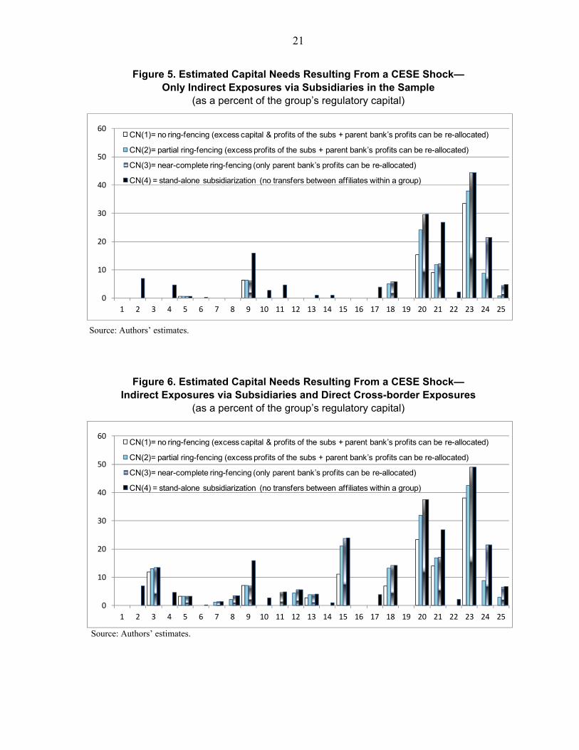
Using the framework and assumptions described above, the capital needs of the sample banking groups are first computed for their indirect CESE exposures via subsidiaries, assuming that subsidiaries have to restore their post-shock CARs back to the regulatory minimum levels. Next, the banking groups’ capital needs are computed for both indirect exposures via subsidiaries and direct cross-border exposures to the CESE region. Finally, the simulations are repeated using a different definition of capital needs for the subsidiaries, namely the amount of capital required for the subsidiaries to restore the post-shock CARs back to the pre-shock (end-2008) levels; because these pre-crisis CARs were generally above the regulatory minimums, capital needs computed under this alternative definition are higher. Focusing only on indirect exposures via subsidiaries, the results are as follows (see Figure 5): (i) Eight out of 25 banking groups have no capital needs related to their CESE
subsidiaries (i.e., CN(4)=0).
(ii) Five out of 25 banking groups have significant capital needs related to their CESE subsidiaries (i.e., CN(4) > 10 percent of the banking group’s regulatory capital). As expected, the capital needs of the banking groups to ensure adequate capitalization of all parts of the group after the shock are higher under near-complete/partial ring-fencing than under no ring-fencing, with the differences being larger for more diversified groups. For example, one of the banking groups (#24), which faces the CESE related capital needs of over 20 percent of its regulatory capital under the SAS model (CN(4)), has zero capital needs under no ring-fencing (CN(1)). In the cases when the parent banks’ profits are zero/negative (meaning that they cannot provide support for their subsidiaries), CN(3)=CN(4). More generally, in the no ring-fencing scenario (which allows reallocation of both excess profits and capital), only five out of 25 banking groups would still face non-zero capital needs after re-allocation, compared to 17 in case of the SAS (where no transfers are allowed within a group).
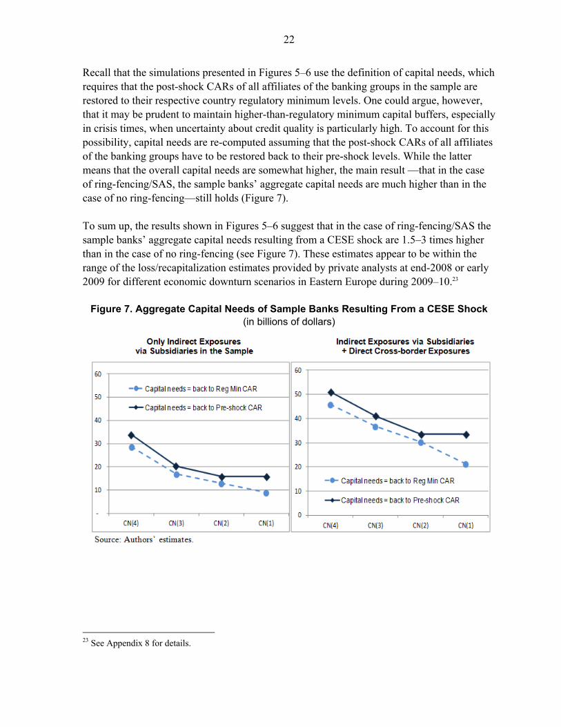
Figure 6 presents the estimated capital needs taking into account direct cross-border exposures and lending via branches, in addition to the exposures via subsidiaries in the sample. While the CN measures in Figure 6 are notably higher than in Figure 5, the results are broadly similar, that is, more ring-fencing entails larger capital needs for most banking groups, with 9 banks (in the no ring-fencing scenario) to 22 banks (in the SAS scenario) in need of extra capital.
21
Figure 5. Estimated Capital Needs Resulting From a CESE Shock— Only Indirect Exposures via Subsidiaries in the Sample
(as a percent of the group’s regulatory capital)
Source: Authors’ estimates.
Figure 6. Estimated Capital Needs Resulting From a CESE Shock— Indirect Exposures via Subsidiaries and Direct Cross-border Exposures
(as a percent of the group’s regulatory capital)
Source: Authors’ estimates.
0
10
20
30
40
50
60
1 2 3 4 5 6 7 8 9 10 11 12 13 14 15 16 17 18 19 20 21 22 23 24 25
CN(1)= no ring-fencing (excess capital & profits of the subs + parent bank’s profits can be re-allocated)
CN(2)= partial ring-fencing (excess profits of the subs + parent bank’s profits can be re-allocated)
CN(3)= near-complete ring-fencing (only parent bank’s profits can be re-allocated)
CN(4) = stand-alone subsidiarization (no transfers between affiliates within a group)
22
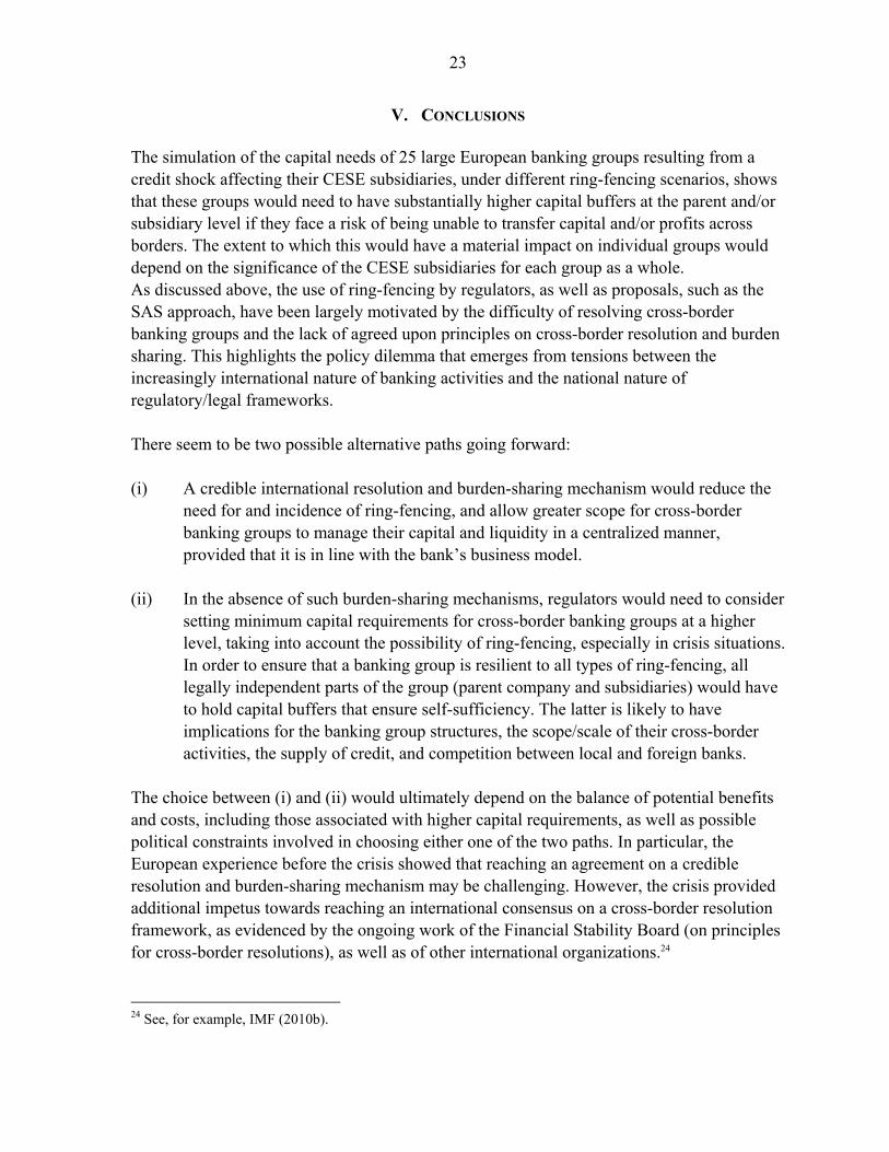
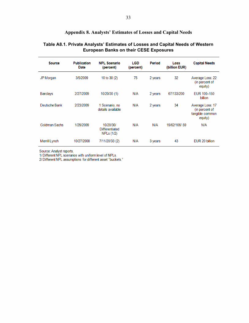
Recall that the simulations presented in Figures 5–6 use the definition of capital needs, which requires that the post-shock CARs of all affiliates of the banking groups in the sample are restored to their respective country regulatory minimum levels. One could argue, however, that it may be prudent to maintain higher-than-regulatory minimum capital buffers, especially in crisis times, when uncertainty about credit quality is particularly high. To account for this possibility, capital needs are re-computed assuming that the post-shock CARs of all affiliates of the banking groups have to be restored back to their pre-shock levels. While the latter means that the overall capital needs are somewhat higher, the main result —that in the case of ring-fencing/SAS, the sample banks’ aggregate capital needs are much higher than in the case of no ring-fencing—still holds (Figure 7). To sum up, the results shown in Figures 5–6 suggest that in the case of ring-fencing/SAS the sample banks’ aggregate capital needs resulting from a CESE shock are 1.5–3 times higher than in the case of no ring-fencing (see Figure 7). These estimates appear to be within the range of the loss/recapitalization estimates provided by private analysts at end-2008 or early 2009 for different economic downturn scenarios in Eastern Europe during 2009–10.23
Figure 7. Aggregate Capital Needs of Sample Banks Resulting From a CESE Shock (in billions of dollars)
23 See Appendix 8 for details.
23
V. CONCLUSIONS The simulation of the capital needs of 25 large European banking groups resulting from a credit shock affecting their CESE subsidiaries, under different ring-fencing scenarios, shows that these groups would need to have substantially higher capital buffers at the parent and/or subsidiary level if they face a risk of being unable to transfer capital and/or profits across borders. The extent to which this would have a material impact on individual groups would depend on the significance of the CESE subsidiaries for each group as a whole. As discussed above, the use of ring-fencing by regulators, as well as proposals, such as the SAS approach, have been largely motivated by the difficulty of resolving cross-border banking groups and the lack of agreed upon principles on cross-border resolution and burden sharing. This highlights the policy dilemma that emerges from tensions between the increasingly international nature of banking activities and the national nature of regulatory/legal frameworks. There seem to be two possible alternative paths going forward: (i) A credible international resolution and burden-sharing mechanism would reduce the
need for and incidence of ring-fencing, and allow greater scope for cross-border banking groups to manage their capital and liquidity in a centralized manner, provided that it is in line with the bank’s business model.
(ii) In the absence of such burden-sharing mechanisms, regulators would need to consider setting minimum capital requirements for cross-border banking groups at a higher level, taking into account the possibility of ring-fencing, especially in crisis situations. In order to ensure that a banking group is resilient to all types of ring-fencing, all legally independent parts of the group (parent company and subsidiaries) would have to hold capital buffers that ensure self-sufficiency. The latter is likely to have implications for the banking group structures, the scope/scale of their cross-border activities, the supply of credit, and competition between local and foreign banks.
The choice between (i) and (ii) would ultimately depend on the balance of potential benefits and costs, including those associated with higher capital requirements, as well as possible political constraints involved in choosing either one of the two paths. In particular, the European experience before the crisis showed that reaching an agreement on a credible resolution and burden-sharing mechanism may be challenging. However, the crisis provided additional impetus towards reaching an international consensus on a cross-border resolution framework, as evidenced by the ongoing work of the Financial Stability Board (on principles for cross-border resolutions), as well as of other international organizations.24
24 See, for example, IMF (2010b).

24
Appendix 1. Capital Adequacy Rates by Country and Bank Type
Table A1.1. Average CARs of Foreign-owned Sample Subsidiaries vs. the Country-Level Average CARs
Country CAR
(Sample subsidiaries) 1/
CAR (Foreign-owned and domestic banks) 2/
Albania
16.4 17.2
Belarus 14.3 21.8 Bosnia 14.0 16.3 Bulgaria 13.6 14.9 Croatia 14.4 15.4 Czech Republic 11.0 12.3 Estonia 15.2 13.3 Hungary 9.4 11.1 Latvia 12.3 11.8 Lithuania 11.5 12.9 Poland 10.9 10.8 Romania 13.7 13.8 Russia 15.0 16.8 Serbia 18.6 21.9 Slovakia 10.0 11.1 Slovenia 11.7 11.7 Turkey 15.8 18.0 Ukraine 16.1 14.0 Cross-country Average 13.5 14.7
Sources: Bankscope and Bank reports (sample), GFSR (country level data). 1/ Authors’ calculations. 2/ Global Financial Stability Report (IMF).
25
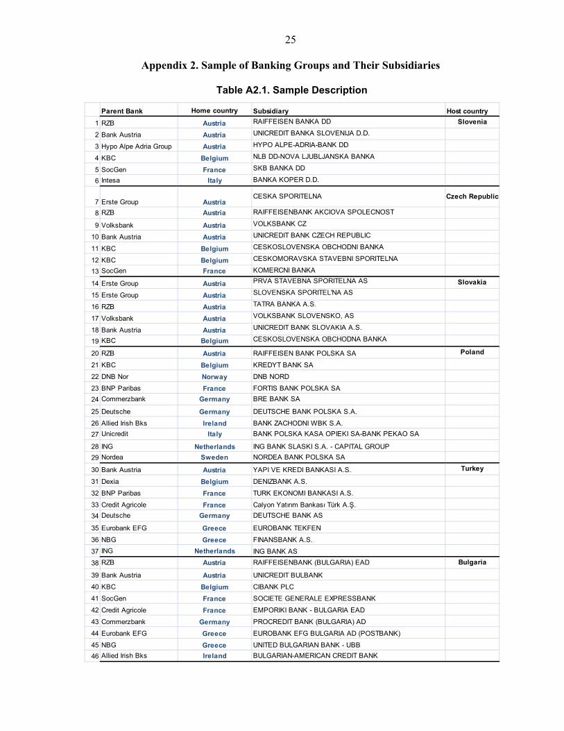
Appendix 2. Sample of Banking Groups and Their Subsidiaries
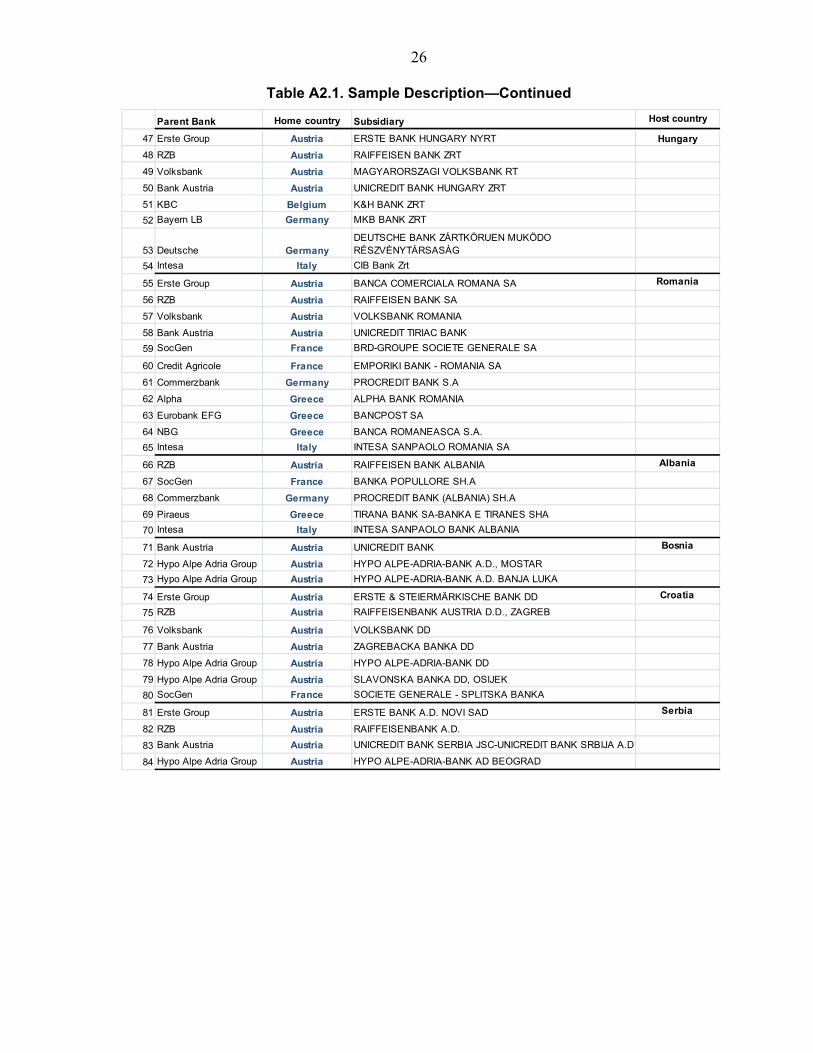
Table A2.1. Sample Description
Parent Bank Home country Subsidiary Host country
1 RZB Austria RAIFFEISEN BANKA DD Slovenia
2 Bank Austria Austria UNICREDIT BANKA SLOVENIJA D.D.
3 Hypo Alpe Adria Group Austria HYPO ALPE-ADRIA-BANK DD
4 KBC Belgium NLB DD-NOVA LJUBLJANSKA BANKA
5 SocGen France SKB BANKA DD
6 Intesa Italy BANKA KOPER D.D.
7 Erste Group AustriaCESKA SPORITELNA Czech Republic
8 RZB Austria RAIFFEISENBANK AKCIOVA SPOLECNOST
9 Volksbank Austria VOLKSBANK CZ
10 Bank Austria Austria UNICREDIT BANK CZECH REPUBLIC
11 KBC Belgium CESKOSLOVENSKA OBCHODNI BANKA
12 KBC Belgium CESKOMORAVSKA STAVEBNI SPORITELNA
13 SocGen France KOMERCNI BANKA
14 Erste Group Austria PRVA STAVEBNA SPORITELNA AS Slovakia
15 Erste Group Austria SLOVENSKA SPORITEL'NA AS
16 RZB Austria TATRA BANKA A.S.
17 Volksbank Austria VOLKSBANK SLOVENSKO, AS
18 Bank Austria Austria UNICREDIT BANK SLOVAKIA A.S.
19 KBC Belgium CESKOSLOVENSKA OBCHODNA BANKA
20 RZB Austria RAIFFEISEN BANK POLSKA SA Poland
21 KBC Belgium KREDYT BANK SA
22 DNB Nor Norway DNB NORD
23 BNP Paribas France FORTIS BANK POLSKA SA
24 Commerzbank Germany BRE BANK SA
25 Deutsche Germany DEUTSCHE BANK POLSKA S.A.
26 Allied Irish Bks Ireland BANK ZACHODNI WBK S.A.
27 Unicredit Italy BANK POLSKA KASA OPIEKI SA-BANK PEKAO SA
28 ING Netherlands ING BANK SLASKI S.A. - CAPITAL GROUP
29 Nordea Sweden NORDEA BANK POLSKA SA
30 Bank Austria Austria YAPI VE KREDI BANKASI A.S. Turkey
31 Dexia Belgium DENIZBANK A.S.
32 BNP Paribas France TURK EKONOMI BANKASI A.S.
33 Credit Agricole France Calyon Yatırım Bankası Türk A.Ş.
34 Deutsche Germany DEUTSCHE BANK AS
35 Eurobank EFG Greece EUROBANK TEKFEN
36 NBG Greece FINANSBANK A.S.
37 ING Netherlands ING BANK AS
38 RZB Austria RAIFFEISENBANK (BULGARIA) EAD Bulgaria
39 Bank Austria Austria UNICREDIT BULBANK
40 KBC Belgium CIBANK PLC
41 SocGen France SOCIETE GENERALE EXPRESSBANK
42 Credit Agricole France EMPORIKI BANK - BULGARIA EAD
43 Commerzbank Germany PROCREDIT BANK (BULGARIA) AD
44 Eurobank EFG Greece EUROBANK EFG BULGARIA AD (POSTBANK)
45 NBG Greece UNITED BULGARIAN BANK - UBB
46 Allied Irish Bks Ireland BULGARIAN-AMERICAN CREDIT BANK
26
Table A2.1. Sample Description—Continued
Parent Bank Home country Subsidiary Host country
47 Erste Group Austria ERSTE BANK HUNGARY NYRT Hungary
48 RZB Austria RAIFFEISEN BANK ZRT
49 Volksbank Austria MAGYARORSZAGI VOLKSBANK RT
50 Bank Austria Austria UNICREDIT BANK HUNGARY ZRT
51 KBC Belgium K&H BANK ZRT
52 Bayern LB Germany MKB BANK ZRT
53 Deutsche GermanyDEUTSCHE BANK ZÁRTKÖRUEN MUKÖDO RÉSZVÉNYTÁRSASÁG
54 Intesa Italy CIB Bank Zrt
55 Erste Group Austria BANCA COMERCIALA ROMANA SA Romania
56 RZB Austria RAIFFEISEN BANK SA
57 Volksbank Austria VOLKSBANK ROMANIA
58 Bank Austria Austria UNICREDIT TIRIAC BANK
59 SocGen France BRD-GROUPE SOCIETE GENERALE SA
60 Credit Agricole France EMPORIKI BANK - ROMANIA SA
61 Commerzbank Germany PROCREDIT BANK S.A
62 Alpha Greece ALPHA BANK ROMANIA
63 Eurobank EFG Greece BANCPOST SA
64 NBG Greece BANCA ROMANEASCA S.A.
65 Intesa Italy INTESA SANPAOLO ROMANIA SA
66 RZB Austria RAIFFEISEN BANK ALBANIA Albania
67 SocGen France BANKA POPULLORE SH.A
68 Commerzbank Germany PROCREDIT BANK (ALBANIA) SH.A
69 Piraeus Greece TIRANA BANK SA-BANKA E TIRANES SHA
70 Intesa Italy INTESA SANPAOLO BANK ALBANIA
71 Bank Austria Austria UNICREDIT BANK Bosnia
72 Hypo Alpe Adria Group Austria HYPO ALPE-ADRIA-BANK A.D., MOSTAR
73 Hypo Alpe Adria Group Austria HYPO ALPE-ADRIA-BANK A.D. BANJA LUKA
74 Erste Group Austria ERSTE & STEIERMÄRKISCHE BANK DD Croatia
75 RZB Austria RAIFFEISENBANK AUSTRIA D.D., ZAGREB
76 Volksbank Austria VOLKSBANK DD
77 Bank Austria Austria ZAGREBACKA BANKA DD
78 Hypo Alpe Adria Group Austria HYPO ALPE-ADRIA-BANK DD
79 Hypo Alpe Adria Group Austria SLAVONSKA BANKA DD, OSIJEK
80 SocGen France SOCIETE GENERALE - SPLITSKA BANKA
81 Erste Group Austria ERSTE BANK A.D. NOVI SAD Serbia
82 RZB Austria RAIFFEISENBANK A.D.
83 Bank Austria Austria UNICREDIT BANK SERBIA JSC-UNICREDIT BANK SRBIJA A.D
84 Hypo Alpe Adria Group Austria HYPO ALPE-ADRIA-BANK AD BEOGRAD

27
Table A.2.1. Sample Description—Continued
Sources: Bankscope, Bank reports, and Analysts’ reports.
Parent Bank Home country Subsidiary Host country
85 SEB Sweden SEB PANK Estonia
86 Swedbank Sweden SWEDBANK AS
87 Bank Austria Austria UNICREDIT BANK AS Latvia
88 DNB Nord Denmark DNB NORD
89 SEB Sweden SEB BANKA AS
90 Swedbank Sweden SWEDBANK AS
91 DNB Nord Norway DNB NORD Lithuania
92 SEB Sweden SEB BANKAS
93 Swedbank Sweden SWEDBANK AS
94 RZB Austria ZAO RAIFFEISENBANK Russia
95 Bank Austria Austria UNICREDIT BANK ZAO
96 KBC Belgium ABSOLUT BANK
97 BNP Paribas France BNP PARIBAS VOSTOK
98 SocGen France BANK SOCIÉTÉ GÉNÉRALE VOSTOK
99 SocGen France JSC ROSBANK
100 Commerzbank Germany COMMERZBANK (EURASIJA)
101 Intesa Italy KMB BANK/ SMALL BUSINESS CREDIT BANK
102 ING Netherlands ING BANK (EURASIA) ZAO
103 Nordea Sweden NORDEA BANK
104 Swedbank Sweden SWEDBANK
105 Erste Group Austria ERSTE BANK OJSC Ukraine
106 RZB Austria RAIFFEISEN BANK AVAL
107 Bank Austria Austria UKRSOTSBANK
108 BNP Paribas France JSIB UKRSIBBANK
109 Intesa Italy PRAVEX BANK
110 ING Netherlands ING BANK UKRAINE
111 Swedbank Sweden PUBLIC JOINT STOCK COMPANY SWEDBANK
112 RZB Austria PRIORBANK Belarus
113 SocGen France BELROSBANK
28
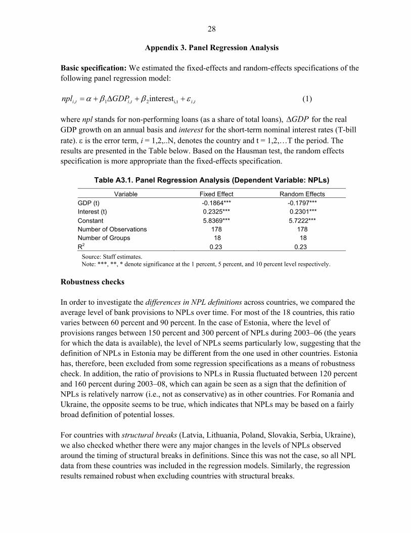
Appendix 3. Panel Regression Analysis Basic specification: We estimated the fixed-effects and random-effects specifications of the following panel regression model:
tititi GDPnpl ,ti,2,1, interest (1)
where npl stands for non-performing loans (as a share of total loans), GDP for the real GDP growth on an annual basis and interest for the short-term nominal interest rates (T-bill rate). is the error term, i = 1,2,..N, denotes the country and t = 1,2,…T the period. The results are presented in the Table below. Based on the Hausman test, the random effects specification is more appropriate than the fixed-effects specification.
Table A3.1. Panel Regression Analysis (Dependent Variable: NPLs)
Variable Fixed Effect Random Effects
GDP (t) -0.1864*** -0.1797*** Interest (t) 0.2325*** 0.2301***
Constant 5.8369*** 5.7222*** Number of Observations 178 178 Number of Groups 18 18
R2 0.23 0.23
Source: Staff estimates. Note: ***, **, * denote significance at the 1 percent, 5 percent, and 10 percent level respectively.
Robustness checks In order to investigate the differences in NPL definitions across countries, we compared the average level of bank provisions to NPLs over time. For most of the 18 countries, this ratio varies between 60 percent and 90 percent. In the case of Estonia, where the level of provisions ranges between 150 percent and 300 percent of NPLs during 2003–06 (the years for which the data is available), the level of NPLs seems particularly low, suggesting that the definition of NPLs in Estonia may be different from the one used in other countries. Estonia has, therefore, been excluded from some regression specifications as a means of robustness check. In addition, the ratio of provisions to NPLs in Russia fluctuated between 120 percent and 160 percent during 2003–08, which can again be seen as a sign that the definition of NPLs is relatively narrow (i.e., not as conservative) as in other countries. For Romania and Ukraine, the opposite seems to be true, which indicates that NPLs may be based on a fairly broad definition of potential losses. For countries with structural breaks (Latvia, Lithuania, Poland, Slovakia, Serbia, Ukraine), we also checked whether there were any major changes in the levels of NPLs observed around the timing of structural breaks in definitions. Since this was not the case, so all NPL data from these countries was included in the regression models. Similarly, the regression results remained robust when excluding countries with structural breaks.
29
Appendix 4. Interest Rates Used for Regression Analysis
Table A4.1. Overview on Data Sources for Short-Term Interest Rates
Country Explanation Source
Bosnia-Herzegovina
Interest rate is constructed as 2/3 times Deposit Rate + 1/3 times Lending Rate, starting in 2002 (other data is not available)
MBTS
Czech Republic Treasury Bill Rate MBTS
Latvia Treasury Bill Rate MBTS
Bulgaria Treasury Bill Rate when available (2 years), otherwise inferred from Interbank Rate (3 months, Bloomberg), otherwise from Lending Rate
MBTS and Bloomberg
Croatia Treasury Bill Rate from Bloomberg (from 2002 onwards), before that: adjust Money Market Rate weighted by the relative portion of T-Bill rates on money market rates from 2002 to 2008
IFTSTSUB (for 1992 to 2001), Bloomberg (from 2002)
Lithuania Treasury Bill Rate (12 months) where possible, otherwise Government Bond Yield (12 months, from Bloomberg), recalculated to 12 months level, otherwise Interbank Rate, recalculated to 12-month T-Bill rate
MBTS and Bloomberg
Romania Interbank short-term lending rate, similar to Treasury Bill Rate (91 days) (which is only available for some years)
MBTS
Slovakia Average Deposit Rate (1993–1999), Government Bond Yield (2002-2006), Government Bond Yield (1 yr, from Bloomberg (2007 to 2009)
MBTS, Bloomberg
Slovenia Treasury Bill Rate (from 1999), before that: Money Market Rate adjusted to Treasury Bill Rate
MBTS
Russia Treasury Bill Rate for 2000–2003, after 2003: avg of money market rate and interbank rate (3 months), before 1999: Money Market Rate
MBTS, Bloomberg
Turkey Treasury Bill Rate, if available; (before 1999: Money Market Rate), after 2007: 1-yr government bond yield.
IFTSTSUB, Bloomberg
Hungary Treasury Bill Rate MBTS
Poland Weighted Average Treasury Bill Rate MBTS
Serbia Money Market Rate IFTS
Ukraine Money Market Rate IFTS
Albania Treasury Bill Rate IFTS
Estonia Money Market Rate IFTS
Belarus Data are scarce; adjusted deposit rates according to money market rates to deposit rates in Ukraine
IFTS
Sources: International Financial Statistics (IFTS), Money and Banking Statistics and Bloomberg.
30
Appendix 5. Regulatory Minimum Capital Requirements by Country
Table A5.1. Regulatory Minimum Capital Requirements in the CESE Countries
Country Minimum Capital Adequacy
Requirements (CARs) (in percent)
Albania 12 Belarus 10 Bosnia 12 Bulgaria 12 Croatia 10 Czech Republic 8 Estonia 10 Hungary 8 Latvia 8 Lithuania 10 Poland 8 Romania 10 Russia 10 Serbia 12 Slovakia 8 Slovenia 8 Turkey 12 Ukraine 8
Source: IMF country desks.

31
Appendix 6. Loss Given Default Ratios in the CESE Countries The country-specific Loss Given Default Ratios (LGDs) are taken from the World Bank Doing Business webpage and are based on work of Djankov et al. (2008). The differences in LGDs across countries reflect the differences in bankruptcy codes, the duration of the proceedings and legal costs. The CESE long-term average LGDs range from 51 percent (Lithuania) to 90 percent (Ukraine). The CESE average of 68 percent is above the LGD for senior unsecured credit under the Basel II Foundation IRB approach (45 percent), which is often used as a benchmark for a through-the-cycle LGD. In order to account for the empirical finding that LGDs increase during downturn periods, we use a formula proposed by the Federal Reserve Board (2006) to derive the downturn LGDs:
Downturn LGD = 0.08 + 0.92 * Long-term average LGD
The downturn LGDs for the CESE countries range from 55 percent (Lithuania) to 92 percent (Ukraine) (Table A6.1). The estimated CESE downturn LGDs are thus substantially higher than those observed for senior bank loans in the OECD countries, which range from 30 percent and 45 percent (see Moody’s 2010, Doing Business database).
Table A6.1. Loss Given Default Ratios by Country
Country Long-term Average LGDs Downturn LGDs
Albania 1/ N/A 70.0
Belarus 66.6 69.3
Bosnia 64.1 67.0
Bulgaria 67.9 70.5
Croatia 69.5 71.9
Czech Republic 2/ 41.3 46.0
Estonia 62.5 65.5
Hungary 61.6 64.7
Latvia 71.0 73.3
Lithuania 50.6 54.6
Poland 70.2 72.6
Romania 71.5 73.8
Russia 71.8 74.1
Serbia 74.6 76.6
Slovakia 54.1 57.8
Slovenia 54.5 58.1
Turkey 79.8 81.4
Ukraine 90.9 91.6 Average 68.3 70.7
Sources: www.doingbusiness.org, and local authorities.
1/ For Albania, the downturn LGD is assumed to be equal to its peer country average
(70 percent); 2/ For the Czech Republic, the average LGD is the one for corporate credit published by the Czech National Bank (CNB 2009, p.81).

32
Appendix 7. Using BIS Data to Capture Remaining Banking Groups’ Exposures to the CESE Countries
The portfolio of subsidiaries included in the sample does not necessarily capture the full CESE exposures of the sample banking groups, as it is missing their direct cross-border claims and lending through their branches in the host countries. In order to capture these exposures, the subsidiaries’ balance sheet data are combined with the consolidated BIS international banking statistics, which reports, at the country level, the consolidated claims of BIS reporting banks on each CESE country. The BIS total foreign claims data (on the immediate borrower’s basis) include both the cross-border claims of foreign banks and all foreign affiliates—subsidiaries and branches—claims. In order to separate direct cross-border and branches’ claims, the domestic lending to customers by sample subsidiaries is subtracted from the total foreign claims (e.g., the customer lending by Greek controlled subsidiaries operating in Turkey is subtracted from the consolidated foreign claims of the BIS reporting Greek banks on Turkish residents). A few caveats need to be highlighted: (i) The residual labeled as “direct cross-border and branches claims” could also include
non-lending claims by subsidiaries, such as government bonds held by a subsidiary. Nevertheless, the potential recap needs calculated for each subsidiary were based on their lending portfolio, and hence, the treatment of other non-lending claims as claims directed linked to the parent bank seems appropriate.
(ii) As documented in other papers, there are some discrepancies between the BIS data and other sources. In our case, we found that there would be a potential small downward bias in the BIS total claims of Italian banks on Ukraine and Swedish banks on Latvia, based on the subsidiaries balance sheet data. This is similar to the discrepancies found by Maechler and Ong (2009) when comparing the BIS data with the central bank data sources. These discrepancies could be due to the differences in the consolidation method and the group structure classification used by different internationally active banks.
(iii) The residual exposure indentified at a parent bank’s home country level is distributed across the sample banking groups of each home country as a proportion of the group’s assets. Since the sample of banking groups in this paper was put together with the objective to capture all major European cross-border banking groups with significant presence in the CESE region, is it unlikely that the BIS data includes a large cross-border banks with operations in the CESE region that is not already included in the sample.
33
Appendix 8. Analysts’ Estimates of Losses and Capital Needs
Table A8.1. Private Analysts’ Estimates of Losses and Capital Needs of Western European Banks on their CESE Exposures

34
REFERENCES Arrelano, Manuel, and Olympia Bover, 1995, “Another look at the instrumental variable
estimation of error-components models,” Journal of Econometrics 68, 29–51. Arvai, Zsofia, Karl Driessen, and Inci Otker-Robe, 2009, “Regional Financial Interlinkages
and Financial Contagion within Europe,” International Monetary Fund, IMF WP/09/6. Babihuga, Rita, 2007, “Macroeconomic and Financial Soundness Indicators: An Empirical
Investigation,” International Monetary Fund, WP 07/115. Board of Governors of the Federal Reserve Bank, 2006, “Basel II Capital Accord—Notice of
Proposed Rulemaking,” September. Cerutti, Eugenio, Giovanni Dell’Ariccia, and Soledad Martinez Peria, 2007, “How banks go
abroad: Branches or subsidiaries?” Journal of Banking & Finance 31, 1669–1692. Czech National Bank, 2009, “Financial Stability Report 2009/2010.” De Haas, Ralph and Iman van Lelyveld, 2010, “Internal Capital Markets and Lending by
Multinational Bank Subsidiaries,” Journal of Financial Intermediation 19 (2010), 1–25 Djankov, Simeon, Oliver Hart, Caralee McLiesh, Andrei Shleifer, 2008. “Debt Enforcement
around the World,” Journal of Political Economy, University of Chicago Press, vol. 116 (6), pages 1105–1149, December.
European Commission, 2010, Study on the feasibility of reducing obstacles to the transfer of
assets within a cross border banking group during a financial crisis, Final Report, April. http://ec.europa.eu/internal_market/bank/windingup/index_en.htm
Hermann, Sabine, and Dubravko Mihaljek, 2010, “The determinants of cross-border bank
flows to emerging markets: new empirical evidence on the spread of the financial crises,” BIS Working Paper no. 315, July.
Hoelscher, David, Michael Hsu, Inci Otker-Robe and Andre Santos, 2010, “Note on Stand-
Alone Subsidiarization Approach and Financial Stability,” manuscript. International Monetary Fund, 2010a, Global Financial Stability Report, April. ———, 2010b, “Resolution of Cross-Border Banks–A Proposed Framework for Enhanced
Coordination; IMF Policy Paper; June 11. www.imf.org/external/np/pp/eng/2010/061110.pdf
35
Institute of International Finance, 2010, “A global Approach to Resolving Failing Financial
Firms: An Industry Perspective,” May. Maechler, Andrea, and Li Lian Ong, 2009, “Foreign Banks in the CESE countries: In for a
Penny, in for a Pound?” International Monetary Fund, WP/09/54. McCauley, Robert, Patrick McGuire, and Goetz von Peter, 2010, “The architecture of the
global banking: from international to multinational?, BIS Quarterly Review, March. McGuire, Patrick, and Philip Wooldridge, 2005, “The BIS consolidated banking statistics:
structure, uses and recent enhancement,” BIS Quarterly Review, September. Moody’s, 2010, Moody’s Global Credit Policy—Corporate Default and Recovery Rates,
1920–2009, Special Comment, February. Popov, Alexander, and Gregory Udell, 2010, “Cross-Border Banking and the International
Transmission of Financial Distress During the Crisis of 2007–2008,” European Central Bank, Working Paper Series No 1203, June.